NBER WORKING PAPER SERIES

ENDOGENOUS ELECTION TIMINGS AND POLITICAL BUSINESS CYCLES IN JAPAN.

Takatoshi Ito

Working Paper No. 3128

NAT1ONAL BUREAU OP ECONOMIC RESEARCH1050 Massachusetts Avenue

Cambridge, MA 02138September 1989

Earlier research for this project was carried out as a joint project with JinHyuk Park, then a senior student at Harvard College when the author was avisiting Associate Professor at Harvard University. An initial set ofempirical results were reported in Mr. Park's senior thesis, and its revisionswere published in Economics Letters. The author of this paper regrets that Mr.Park could not participate after his graduation in continuation of the project1developing a theoretical part. The present author would like to take a fullresponsibility for errors of this paper, but Mr. Park shares credits inempirical parts of this paper. This author is grateful to a support given tothis project by the Department of Economics, Harvard University. Discussionswith David E. Bloom, Christopher Cavanough, Barry Eichengreen, RidehikoIchiisura and Ken Wolpin have been helpful. This paper is part of NBERsresearch project in Financial Markets and Monetary Economics. Any opinionsexpressed are those of the author not those of the National Bureau of Economic

Research.

EThER Working Paper No. 3128September 1989

ENDOCENOUS ELECTION TIMINGS AND POLITICAL BUSINESS CYCLES IN JAPAN

ABSTRACT

This paper constructs a theoretical model of political

business cycles in a Parliamentary system and tests predictions

and hypotheses of a theoretical model against the post-war

Japanese data. Unlike in a presidential system, the timing of a

general election is an endogenous policy variable in a

parliamentary system. Thus, one of the interesting questions in a

parliamentary system is whether elections cause business cycles

or economic expansions trigger general elections.

Empirical analyses of the post—war Japanese experience

strongly indicate that the Japanese government did not manipulate

policies in anticipation of approaching elections as political

business cycle theories in a presidential system indicate.

Instead, general elections were usually held during times of

autonomous economic expansion. In other words, the Japanese

government opportunistically manipulated the timing of elections

rather than the economy.

Takatoshi ItoInstitute of. Economic ResearchHitotsubashi UniversityKunicachi, Tokyo 186JAPAN

I. Introduction

This paper constructs a theoretical model of political

business cycles in a parliamentary system and tests against the

postwar Japanese data predictions and hypotheses derived from the

theoretical model. Unlike in a presidential system, the timing of

a general election is an endogenous policy variable in a

parliamentary system. Prime Minister in Japan may dissolve the

House of Representatives anytime during its four-year term''

Thus, one of the interesting questions in a parliamentary system

is whether elections cause business cycles or economic expansions

trigger general elections.

Empirical analyses of the post-war Japanese experience

strongly indicate that the Japanese government did not manipulate

polidies in anticipation of approaching elections as political

business cycle theories in a presidential system could indicate.

Instead, general elections were usually held during times of

autonomous economic expansion. In other words, the Japanese

government opportunistically manipulated the timing of elections

rather than the economy.

Models of political business cycle theories with myopic

voters start from the underlying premise that the electorate has

preferences among economic outcomes that are reflected through

its voting behavior. Low unemployment, low inflation and high

output garner more votes for an incumbent partyo However, voters

are also presumed to be myopic: In evaluating the general state

—1—

of the economy, they take into account only recent past

experiences without any future expectations. Politicians, only

interested in winning elections without much regard for the

welfare of the society, thus stimulate an economy before the

election at the cost of post-election inflation. As politicians

try to exploit the trade-off in the short-run Phillips curve

every four years, business cycles are created.

The literature in this strand can be classified along two

lines: The traditional theory by Nordhaus (1975) and Tufte

(1978); and the partisan theory by Hibbs (1977, 1987), Beck

(1982), and Alesina and Sachs (1988).'2 According to Nordhaus,

an incumbent party generates expansions near elections and then

induces contractions to control the overheated economy after the

election. Hibbs and his followers, on the other hand, emphasizes

the partisan nature of politics. He argues that parties with

different core constituencies pursue different economic policies.

The change in parties cause the change in social priorities.

Recently, models with rational voters have been developed,

with two lines of thoughts. Cukierman and Meltzer (1986) and

Rogoff adn Sibert (1988) considered a model in which political

parties, whose objective is to maximize the probability of

staying the power, faces rational voters who rationally expect

how political parties possibly manipulates the economic policies

for elections. Alesina (1987) and Alesina and Sachs (1988)

investigated models with two parties with different social objec-

—2—

tives play repeated games and test against the U.S. postwar data.

Most of these works have been conducted in the framework of

the U.S. presidential system, in which elections come once every

four years. Careful applications of the idea to other countries,

taking into account a different political system, are scarce. In

fact, in the parliamentary system like one in Japan, the timing

of elections is not fixed, but subject to a discretion of Prime

Minister. Instead of manipulating an economy in an attempt to

line up the peak of business cycles to the fixed election timing,

the incumbent party may opportunistically wait for a business

cycle peak which is generated by autonomous forces of private

sectors.

An investigation on political business cycles in Japan is

important in several aspects.\-1 First, the Parliamentary nature

of the Japanese government requires us to construct a model which

allows for endogenous election timings. Although political

business cycles in Britain, as a part of cross-country studies,

have been investigated earlier, no rigorous theoretical framework

for a parliamentary system was proposed. In section 3, I will

propose a general model which describe interaction between

election (timing) and business cycles.

Second, election timings are chosen by policy makers

depending on the course of the economy, while the policy is

conducted in expectation of elections. This implies that the

simultaneity bias becomes a problem in estimating effects of

—3-.

economic performance on election timing and effects of expected

election on policy manipulation. We will empirically answer the

question whether elections cause booms or booms trigger elections

in Japan, correcting for the simultaneity bias. Inoguchi (1983)

was the first to emphasize endogeneity of election timing in

Japan. He concluded that it was more likely that the Japanese

government seized the opportunity of good economic performances

to call a general election. He attributed his finding in part to

a strong bureaucratic system independent from political

influences. Although his insight was novel, his conclusion was

not based on rigorous estimation procedures and hypothesis

testings. \

Ito and Park (1988) devised an econometric test of the

endogeneity of election timings. They investigated whether

economic variables influenced the probability of election

timings, given the time elapsed from the last election. They

found a significant effect of unexpected better performance of

the economy on the probability of election. They have also tested

whether monetary and fiscal policies were manipulated in the

expectation of electjons. They did not find an evidence that

economic policies were manipulated.

Cargifl and Hutchison (1988) also investigated whehter the

probability of elections was influenced by economic performances.

They came down to an opposite conclusion from Ito and Park: "the

incumbent party does not appear to systematically use generally

—4-.

good economic conditions (or news of these conditions) in its

decisions to call elections early." In the subsequent paper,

Cargill and Hutchison (1989) examined whether the reaction

function of monetary policy (captured by the interest rate or themoney supply) of Bank of Japan was influenced by the electiontimings (dummy variable), and found that after 1975, the Bank of

Japan a systematic downward shift in the interbank rate preceding

Lower House elections. Moreover, the effect is. tempered by the

strength of the incumbent party..

The rest of this paper is. organized as follows. Next

section will make . an informal observation at the relationship

between the growth rate and the, election timing. Section 3 will

present a theoretical. model in which the election timing is

optimally chosen by the government. An empirical analysis of the

traditional theory (effects of elections on policy manipulations)

will be carried out in section 4. A hypothesis that election

timing is endogenously chosen will be tested in section 5.

II. Casual Observations

Suppose, as uaual, that the government tries to call an

election in a quarter with good economic performances, say, the

growth rate. Then we should expect to find that the growth rate

tends to be higher in election quarters. Now recall the

Constitutional constraint that the general election has to be

called before the end gf four-year (16 quarter) term. Suppose

also that the government cannot manipulate economic performances

—5—

with certainties. Under uncertainty, the government would call

an election near the end of the four-year term even if the growth

rate is only moderately high, because time may run out on the

incumbent without a quarter of a very high• econmic growth rate.In sum, we expect that the probability of election tends to

increase with growth rate and to increase as the number of

quarters since last election (TSLE) increases. In other words,

an election called relatively early in the term is accompanied by

a very high economic growth rate and an election called near the

end, of the term may be accompanied by a moderately high economic

growth rate.Hence, when we plot the growth rate of each election

cycle (y-axis) against the number of quarters elapsed' (x—axis),the end of election cycles (election timing) tend to be downward

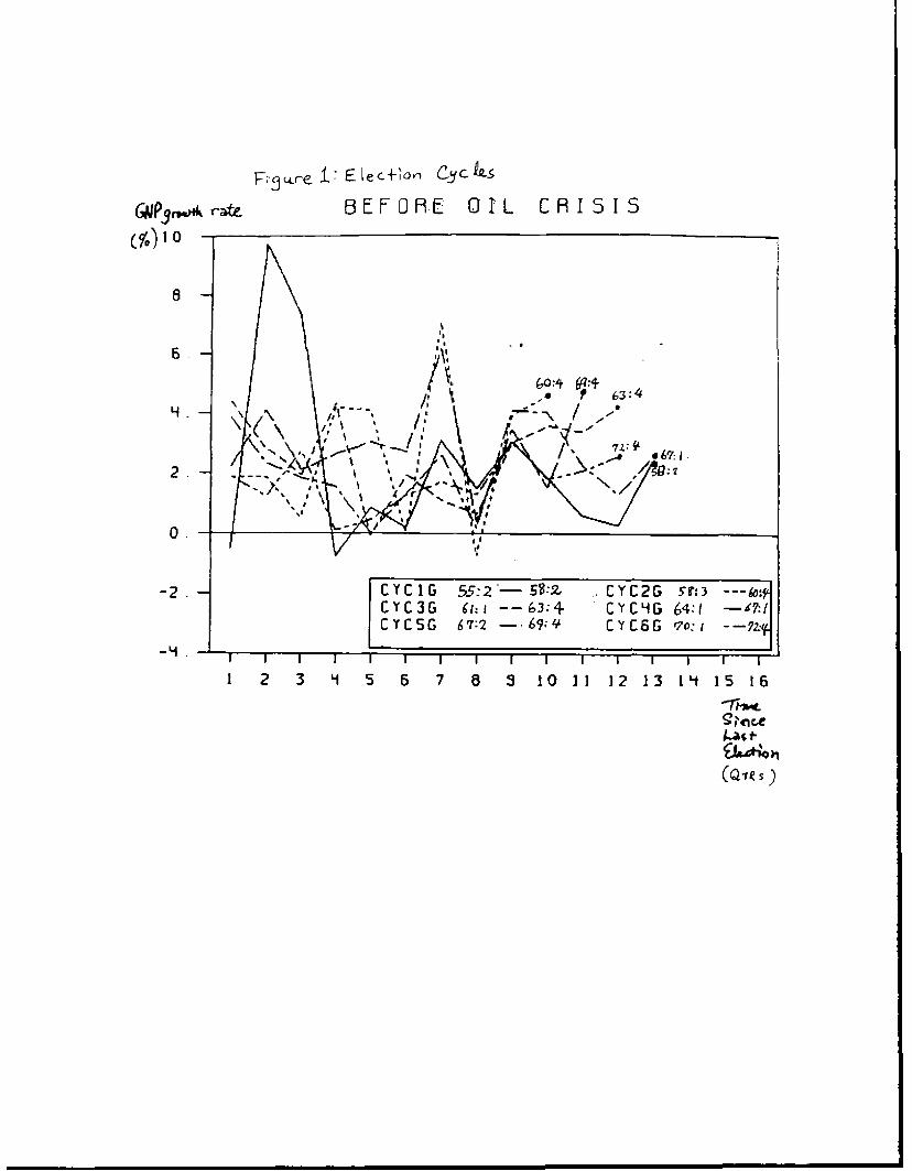
slongFigure 1 (1955—1972) and Figure 2 (1973—1906) show

relationship between the election timing, as a function of the

number of quarters since last election and the growth rate.

samples are divided into two periods, before and after the first

oil crisis. Samples before 1955 are not used, because the

formation of Liberal Democratic Party (LDP) via merging two

parties in 1955 changed the political structure.

Insert figures 1 and 2 here

In Figure 1, the downward-sloping election threshold is

evident. Elections called between 10th and 11th quarters since

—6—

last elections are accompanied by growth rates exceeding 4

percent. When the term went into the 4 year (13th quarter), the

election was called at the growth rate as low as 2 percent.

However, in each case, the growth rate of each election quarter

is higher than the preceding quarter. Moreover, the plot of

election quarters (marked by dots and quarter identifications)

show the downward-sloping property predicted in the earlier

discussion in this section.

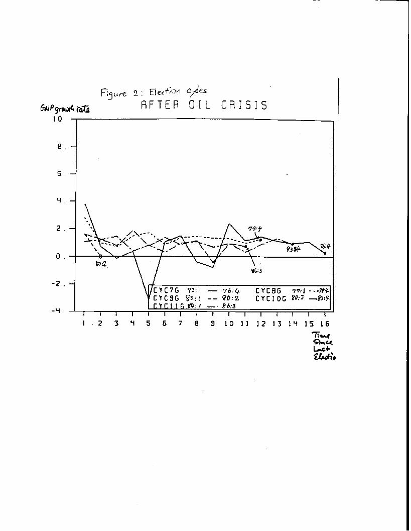
In Figure 2, the downward-sloping property is not evident.

The first election cycle after the first oil crisis went to the

full four—year term for the first time. It is likely that the

government did not realizes that the structural change had

occurred so that the growth rate is permanently lower. The

government waited for a high growth quarter, and waited. But it

never came. In retrospect, the government should have called an

election in the 10th quarter, when the growth rate was 2.4

percent, which was much lower than the election threshold of the

pre-oil shock phase (Figure 1), but which turned out to be much

higher than the subsequent quarters. The election cycle started

in 1980:1 lasted only a half year. Clearly this was not a good

time to have an election: it was a low growth rate and too early

in the election cycle. However, this early dissolution was due

to an "accidental" passage of the nonconfidence vote on the hira

cabinet. Hence, this election cycle is an outlier from our

viewpoint of political business cycles.

—7—

III. Endoqencus election tining: An Example

In the preceding section, an observation was made that an

election was called at a lower growth rate if the number of

quarter since last electiOn was greater. In this section, I will

develop an theoretical example in which an optimal decision of

the government produces the choice of election timings with the

observed characteristics.

Suppose that the full term of House of Representatives are

four periods (years). The number of periods elapsed since last

election is denoted bys. Suppose that the economic growth rate,

is the only relevant variable for voters in the election, and

there are only three possible states with regard to g, High

growth, moderate growth, gM, and low growth gt, with an equal

probability, 1/3, each. The growth rate at the time of last

election is denoted by g0

Every period, the government observes the growth rate, g5,

and decides whether to call an election. If the government

calles an election in a period with the growth rate g, the

political value of the election is the expected value of being

the power in the next election cycle. Let us denote by V(g5) the

political value of calling an election in a period with growth

rate g5. The value will be calculated later as a value functiOn

of dynamic programing problem. An election in a high growthperiod will make an incumbent party to win with a wide margin,

yielding the political value of h: V(g11)h. Elections in a

•Lec-2.txt . S -

moderate growth rate would make an incumbent party to win with asmall margin, yielding the political value of m: V(gM)nm. ir an

election is held in a low growth period, the incumbent party is

assumed to lose a majority, and the opposition takes over a

government with a moderate margin. The fixed value, -k,

represents the agony of defeat and the discounted sum of expected

political values being as an opposition party: V(gL) = -ic.

If the incumbent party decides not to call an election, the

party extracts political utility to be in the power, b(g0, s).

The utility is a compoSite of psychic satisfaction and the

financial donation from the private sector to the party. The

utility is an increasing function of g0 since the maintaining a

wide margin gives an easy management of the govenment and the

House of Representatives. The utility is decreasing function of

s, because the returns to be in the power will deminish.

Thus, let us assume the utility of staying power in the s-

period after the election is,

s) = b1/s, s= 1,2,3: and b(gM, s) = bM/s, s= 1,2,3.

Note that the election with the low growth rate ga implies the

loss of majority. ThéreiS no b assigned for this case, since

the fixed political value of election, -k, already takes into

account the value being outside the power.

Now we are ready to describe the dynamic probramirtg program,

sumsarized in chart 1, which will solve the value function V(.).

etec2.txt - 9 -

chart 2.

-- thserve 1' bCg091)--> cSern 2' b(g012)•-n*serve 03. b(%.3)--'b(5013)sd eLection / and etect Ion / and eLection /

decision -- no / decision -- no / decision -- no / full termI yes\ -- yes\ -- yes\ electionLast Velection VC92) V(03) Via4)V(g0)

sote: VCç) a h. rn d -k if a j, 0N, ad respectiwly.

Case 1: The last election at

Suppose that the last election was held in a high growth

period. We calculate the polical value of the last election by

calculating the value backwards.

In the fourth period since the last. election (s=4), another

election must be held, so that the expected (period 3) value for

the fourth period is

5=4) h/3 + m/3 - k/3 = (h-I-m-k)/3.

In the third period, if an election is not held, the utility of

staying in power b/3 is earned in that period and the expect

value EV(g4, h) is also earned: the sum being (b+m+h-k)/3. If an

election is chosen, the political value of election V(.) is

earned depending on the state of economy. The election decision

is made. Let us assume, for example,

h > m > (bM+h+m-k)/3 > -k. (1)

This implies that in the .third period after election1 thehigh or

moderate economic growth would trigger an election. But the low

growth will. not. Given this condition, the expected value of the

- 10 -

third period is

EV(g0=g, s=3) = h/3 + m/3 + (bH+h_k)/9= (bH+4h+4m_k)/9

The second period decision problem is similar: Knowing g2, the

government calls an election if V(g2) > b/2 + EV(g0=gM, s=3).

The right hand side of this inequality is the sum of the value of

staying in power during the second period and the expected value

of going into the third period. Let us assume, for example,

h > (llb0 + 8h ÷ 3m — 2k)/18 > n > -k (2)

Then, an election option is chosen only if high growth is

achieved in the boom in the second period. Moderate and low

growth will make the incumbent government to wait and see, while

the government enjoys commanding the power. The expected value is

then

EV(g0=g, s2) = h/3 + (2/3) (lib + 8h + 3m - 2k)/lB= (llb + l7h + 8m - 2k)/27

The decision problem at the beginning of the first period is to

compare bH + EV(g0=g1 s=2) with V(g1). Assume that

(38b1 + ]7h + Sm — 2k)/27 > h (3)

Then, an election is not called even with high growth in the

first period after the last election. Therefore, the expected

value is

EV(g0=g11, s=l) = (38l + l7h + Sm — 2k)/27

Now the value of V(g'1)=h is endogenously solved by equating the

value of having an election (s=O) in a high growth period is the

e(ec-2.tn 11 -

expected value of this government in the future.

h = EV(g0=g, s=l) - c

= (3ab + l7h + Sm — 2k)/27 — c (4)

where c is the cost of election incurred by having an election.-

case 2: The last election at bM

Suppose that the last election was held at a moderate growth

period. The expected value for the fourth period is the same as

Case 1:

EV(90=qN, s=4) = h/3 + m/3 - k/3 (h+m-k)/3.

In the third period, if an election is not carried out, the

utility of staying in power bM/) and the expect value EV(g0=gM,

s=4) is also earned. Note that we assume b > bM. If an

election is carried out, the political value of election V(.) is

earned. Observing and comparing V(g) with (bM+h+m_k)/3, the

election decision is made. Let us assume, for example,

h > in > (bM+h+m_k)/3> —ic. (5)

This implies that in the third period after elections the high or

moderate economic growth would trigger an election, as was in

Case 1. With this decision rule being known, the expected value

is

EV(g0=gM, s=3) = (bM+4h+4m_k)/9.

In the second period, the no—election option would produce

the value bM/2 + EV(g0=gM, s=3) = (llbM + Sh + Sm - 2k)/lsp. Let

us assume that

•(ec2.txt - 12 -

Ii > in > (llb + 8h + 8m - 2k)/18p > —k (6)

Then in the second period, the election is called unless growth

is in the low state. Then, the expected value is

EV(g0=gM, s=2) = h/3 + m/3 + (1/3)*(llbM+8h+8m_2k)/ls.= (ll,54)bM + (13h+13m—k)/27

In the period 1, the value of no election is bM + EV(g0=gM, s=2).

Let us assume

h > (65*bM)/54 + (lJh + 13n — k)/27 > in > —k (7)

Therefore, if growth is high, an election is called even in the

first period in Case 2 (unlike Case 1).

EV(g0=gt, s=l) h/3 + (2/3)*(65bM+26h+26m_2k)/54.

(65/81) ibM + (53h+26m—2k)/81.

Now the value of in is the expected sum of the future political

values less the election cost c:

in = (gc't s=l) - c

(65/81) *bM + (53h+26m—2k)/81— c. (8)

Case 3: The last election at

If an election is called in the low growth period, the party

loses the majority, and the opposition party takes over as a

moderate winner.

where P is the average length of staying as an opposition party,

and bL is the per period value of being an opposition party;

bL<bM. (9)

Since P > 0, (9) would be satisfied if

rtec-2.txt - 13

bM > 0 > (9')

Solution

The political values of calling an election in high and

moderate are thus calculated endogenously and simultaneously by

equations (l to (9). The solution to the above problem is said

to exist, if we find parameter values, bH, bM, b', h, m, k, and

c, satisfying all inequalities (l)-(3), (5)-(7), and (9) and

equalities (4) and (8).

A simulation program to find such a solution can be easily

constructed by first assigning values to bH, bM, k, and c, and

second, solve from (4) and (8) for h and m. Then check whether

inequalities- (l)—(3), (5)—(7), (9') are satisfied. For example,

the following values satisfy all the conditions (l)—(8), and

(9'):

c=5, k=30, bH=20, iiLio; then (4) and (8) are solved for h and n;

h = 258.373..., m — 252.3413

It is easily verified that inequalities (1)—(3), (5)—(7), (9')

are satisfied.

Election decisions, solving an example of dynamic programing

problem described above, are illustrated in Figure 1. Call an

election (0) or No election (x) is indicated as a function of the

growth rate g and the elapsed time since last election s. From

this figure the following two properties in analogy of search

theory are observed.

.tec-2.txt

Insert chart 2 about here

Property 1: (Reservation growth rate property of election timing]

In period s, if an election is called for g5, then it would

also call an election for any g which is larger than g5.

Property 2: (Declining reservation growth rate property of

election timing]

If an election is called for g5 in period s, then the

election is also the choice f or g5 in period sf1.

These properties were evident in Figures 1 and 2, especially

the former. Now we have just shown that a simple theoretical

model will yield the same properties. Of course, the above

theoretical framework has a lot of simplifying assumptions.

However, it remains my conjectures that these properties will

hold in a generalized framework. It is a topic of future

research.

e(,c-2.txt - 15 -

chart 2: Optimal Election Decision rule:

Assumption:

ca5, ka30, b=2O, 1inlO; then (4) and (8) are solved for h and m;

h = 258.373... m = 252.3413

case 1 TI tM last election was called in high growth period.

growth raterealization

p.

X 0 0 0

g?1 x x o o

gL x x x o

> S1 2 3 4

o Call an electionNot to call an election

case 2 fl the last election was called in moderate growth period.

growth raterealization

0 0 0 0

gM x o o o

gL x x o

> 51 2 3 4

o : call an electionx : Not to call an election

n(c2.tn - 16 -

IV. Empirical Results: Traditional Political Business Cycles

A. Popularity Punction

The first step of traditional political business cycles

theory is to find economic variables which voters are watching to

judge the competence of the incumbent party. Natural candidates

of relevant economic variables include, among others, the

economic growth rate, and the inflation rate. The unemployment

rate has been used in the U.S. study, but we do not use this

variable, since the Japanese unemployment rate has been

insensitive to business cycles. An additional dummy variable is

used to distinguish House of Representatives elections that were

held at the same time with Mouse of Councillors elections. They

were called the Dojitsu (same day] elections, or the double

elections. It has been widely believed that a Dojitsu election

helps the LDP draw its passive supporters to the polling place,

because voters recongnize a higher significance and feel a

greater satisfaction from voting, given the transaction costs to

the poll.

Now, the popularity function is specified as a percentage of

seats captured in a general election as a function of the GNP

growth rate, g, and the inflation rate, p, and the Dojitsu

dummy, D)

= a1 + a2T + baDt + b1g + b2pt + 4

where v denotes the percentage of seats won by the incumbent

party (LDP), and T denotes the trend. Theory predicts that b1 is

elec-3.txt 17 -

positive and is negative. If voters' memory for policy

evaluation is extremely short then the use of quarter—to-quarter

growth (and inflation) rate is appropriate. Cases with the one-

year, two—year and three—year memory are also examined.

Table 1 about here

Results are shown in Table 1. All signs are consistent with

priors and theory. There is a long-term decline in LDP support

and the Dojitsu election really helps the LOP gaining votes. An

influence of the GNP growth rate on votes is positive and

significant in short-memory versions up to two years and an

influence of Inflation rate on votes is always negatively and

significant. These findings are consistent with a popular thesis

of the traditional political business cycle theory (with myopic

voters).

The horizon of voters' evaluation seems to be less than two

years. Although we do not conduct a formal test of length of

memory due to a lack in the degree of freedom, it is not

inappropriate to assume that evaluation include variables in the

past year only. The finding of short memory justifies the use of

a theoretical model in the preceding section.

B. Policy manipulation

In this section we examine whether any visible changes

(beyond seasonal and demand factors) exist in monetary and fiscal

policy occurred around the election time. An idea is to test

elec-3.cxt . 18

whether an election would cause the government to conduct

expansionary monetary and fiscal policies.

As policy tools, we selected the money supply (M2+CD) growth

rate, and the ratios of government consumption and expenditures

to GNP. The choice of M2+CD is natural, because Bank of Japan

watches M2+CD as opposed to Ml as an important monetary aggregate

after 1975 (See Ito (1988)). The dummy variable for the regime

change will be introduced.

The government consumption or investment represents a fiscal

side of government discretion. Political favors in Japan often

take a form of bringing public projects for constituents.

Moreover, government transfers, which have been used in the

literature, are a difficult figure to obtain in Japan, since many

relevant transfers are done in the local level rather than the

central government level. The Japanese government investment

share of ON? is much higher than the United States, and it is an

important policy variable. The tax burden and transfer payments

do not adequately reflect the fiscal policy being pursued.

Hence1 only government investment (GI) and consumption

expenditures (GC) are included in our fiscal reaction functions.

The GI/GNP or GC/GNP ratio is adopted as the fiscal measure.

First, a naive approach of including an election dummy on

the right hand side will be estimated. If the election quarter

is exogenously determined and perfectly known to the monetary and:

fiscal authorities, then the use of election dummy variable is

elec-3.txc - 19

justified. If there is a lag between policy manipulation to the

result of an economy, then manipulation may occur in the period

preceding to the election quarter4 Hence, the election dummy,

ELEC(t) or ELEC(t-l) is used in the estimation.

However, the naive approach of using an election dummy

would suffer from the simultaneity problem, if the (result of)

manipulation affect the election timing. The simultaneity bias

can be avoided if we use exogenous variables which would predict

the (unconditional) probability of elections. Namely, the time

(in number of quarters) elapsed since last election (TSLE) can be

used for this purpose. Alternatively, the ga post probability

distribution of post—war elections (PREL) as a function of TSLE

can be used, when voters are assumed to have a knowledge of such

a probability distribution.

(1) Monetary policy

The monetary policy is specified as follows:

! ajDj + a5REGIME+ b1jm_j + b2pt_t + b3g_1 + b4Et + 4where mt is the quarterly growth rate of M2+CD money supply, t) is

a vector, (constant, trend, 2nd qtr dummy, 3rd qtr dummy, and 4thqtr dummy); and REGIME is a dummy for regime changes describedabove (1 after 1975:1)); '— is the annual inflation rate forfour quarters, is, the one—year moving average of the

quarter-to-quarter CUP growth rate; and Et is a election

variable, namely ELECt, ELECt+i, TSLEt, or PRELt, and 4 is the

disturbance term.

elec.3txt - 20 -

Estimation results are summarized in Table 2, panel A. For

any of the four election variables, art election variable has an

insignificant coefficient. The table reveals no evidence for

manipulation of monetary or fiscal policies in expectation of

upcoming elections. It does not provide us with any support for

the traditional line of political business cycle theory. In

other words, the insignificant coefficient of the value of

election dummy, E, casts a doubt on monetary manipulation in

Japan.

Table 2 about here

(ii) Fiscal Policy

The fiscal policy in Japan has gone through a significant

regime change just as the monetary policy did. The Japanese

government pursued balanced budget principle until 1965.

Although deficit financing became legal in 1965, it was not until

the mid-l970s that the debt-GNP ratio had skyrocketed in an

attempt to combat contractions due to the first oil crisis. Yet,

the government budget share of national income remained at a

relatively low level compared to those of other countries. We

will introduce a dummy variable after the first oil crisis in

part to capture the structural change in debt policy in the mid-

1970s. The fiscal policy manipulation is specified as

2 aiDs + a6OIL + 'b1ft_i + b2g...1 + b3Etwhere t is a measure of fiscal policy: Cl/GM? or Cc/CM?; OIL is

elec'.3.txt - 21 -

the first oil crisis dummy (1 after 1974:1); and other right—

hand-side variables are the same as the monetary manipulation

equation.

The estimation results are summarized in Table 2, panels B.

Again, there is no evidence to the hypothesis that the

probability of an upcoming election, represented by ELEC, TSLE or

PRE1, influenced the government consumption or investment.

In sum, we do not detect any influences of election

(probabilities) perceived by a function of the elapsed time since

last election on the conduct of either monetary or fiscalpolicy

in Japan.

V. Opportunistic Government Hypothesis

Section 2 and 3 provided the casual observation and a simple

theoretical model for a hypothesis that election timings are

endogenous, or, to put simply, booms trigger elections, while the

evidence in section 4 suggests us that the traditional causality

in the literature, namely election causes booms, is not detected

in Japan. In this section, we will develop an econometric test

to nest the two hypotheses in the same equation.

A. Preliminary Investigation

It is our hypothesis that an election timing depends on

economic growth, g, inflation, p, and the number of quarters

elapsed since last election, TSLE. However, due to the possible

missing variables, such as political events, the relationship

elec-3.txt - 22 -

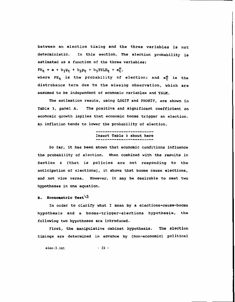
between an election timing and the three variables is not

deterministic. In this section, The election probability is

estimated as a function of the three variables:

PEt a + b1g + b2p + b3TSLEt +

where PEt is the probability of election; and 4 is the

distrubance term due to the missing observation, which are

assumed to be independent of economic variables and TSLE.

The estimation resuts, using LOGIT and PROBIT, are shown in

Table 3, panel A. The positive and significant coefficient on

economic growth implies that economic booms trigger an election.

An inflation tends to lower the probability of election.

Insert Table 3 about here

So far, it has been shown that economic conditions influence

the probability of election. When combined with the results in

Section 4 (that is policies are not responding to the

anticipation of elections), it shows that booms cause elections,

and not vice versa. However, it may be desirable to nest two

hypotheses in one equation.

B. Econotuetric Test

In order to clarify what I mean by a elections-cause-booms

hypothesis and a booms-trigger-elections hypothesis, the

following two hypotheses are introduced.

First, the manipulative cabinet hypothesis. The election

timings are determined in advance by (non-economic) political

elec4]txt - 23

reasons, which econometricians do not know. Although the length

of election cycle in a parliamentary system does vary, it works

like the presidential system if the timing is known to the

government in advance. The government manipulates the economy

through monetary and fiscal policies in an attempt to cause a

boom without inflation at the time of election.

Second, the opportunistic cabinet hypothesis. The incumbent

government does not use monetary or fiscal policy- in order to

influence the economy, just because of an election. The

incumbent waits for a timing in that some non-government, septor

shocks cause high growth and low inflation. The Japanese

incumbent cabinet has four years to grab a right moment. The

threshold of calling an election as a function of economic

performance would change as the full term approaches.

The proposed test of manipulative vs. opportunistic

government requires the econometrician to decompose growth and

inflation into policy-induced parts and non—government sector

shocks. We assume that the former is captured by the expected

component of actual growth and inflation, while the latter is

captured by the unexpected part. Each of the growth and

inflation equations is regressed on the constant, trend, money

growth (1 to 6 lags), government consumption and government

investment. (Results are not reported here. Then the fitted

values, as the effect of growth and inflation due to policy

manipulations, and residuals, as the effect of non—government

elec-3.txt - 24 -

Footnotes

1. A general election could be called in three different

reasons. First, a general election must be held, if not earlier,

at the end of a four—year term of Lower House members. Second,

an election can be called if Prime Minister voluntarily dissolves

the Lower House. Prime Minister could find some excuses to

dissolve the Lower House if he thinks that the timing is

politically advantageous. Third, if the Lower House passes a

non-confidence resolution against the cabinet, then the Prime

Minister has to either disesolve the Lower Rouse or resign. If

the latter, the Lower House elects new Prime Minister without a

general election.

The Japanese Parliament or the Diet, which closely resembles

the British system, is divided into two houses; the Rouse of

Representatives (Lower House) and the House of Councilors (Upper

Rouse). The head of the government, Prime Minister, is elected

by the election among the member of the Lower House.

Traditionally, the head of a majority party (or a coalition of

parties) becomes Prime Minister. Also a majority of Cabinet

members are required to be selected from the Lower House. On

occasions when the two houses are in conflict, the Lower House

usually commands more power. TherEfore, the Lower House carries

more political power than the Upper House. The election of the

Lower House members, the general election, is the most important

political event.

elec-fn.txt — 1 —

The Liberal Democratic Party (LDP) has dominated both houses

since its creation by merging the Liberal and Democratic parties

in 1955. The ruling party has an incentive not only to achieve

the majority but also maximize the number of seats in the House,

since the management of the House is much easier with a wider

margin. Therefore, although the LDP has maintained a majority

most of the time, it is reasonable to assume that the party has

pursued an objective of maximizing the seats in the House.

2. Golden and Poterba (1980) and Frey and Schneider (1978) have

estimated the so-called popularity function in order to test

whether the President's popularity depends on economic

conditions. Golden and Poterba also models how the government

uses fiscal and monetary instruments to produce political

business cycles and rejects Nordhaus' theory. Similarly,

MoCallum (1978) finds no support for the hypothesis. MacRae

(1977) enalyzes whether the electorate is myopic or not. To

examine the welfare consequences of the traditional hypothesis,

Chappell and Keech (1983) construct a complete macroeconomic

model and concludes that the six—year presidential term generally

entails less social welfare loss.

3. Japan is an excellent testing ground for the theory of

political business cycles, since the business and government are

said to enjoy much closer relationship than in the United States.

Management of business cycles (either creating one or taming one)

is presumably easier in Japan than the United States.

elec—fn.txt — 2 —

sector shocks, from these equations are used in the probit and

logit equations of election timings. If the manipulative cabinet

hypothesis is the case, then the coefficients on the policy—

induced growth and inflation are significant; if the

opportunistic government hypothesis is correct, then the

coefficients on the non-government sector shocks are significant.

Results of this test is reported in Table 3, panel B. The

results strongly suggest that the demand and supply shocks,

independent from policy, tend to trigger elections. In

particular, there is more likely to be an election (i) when the

surprise growth rate is higher: (ii) when the surprise inflation

rate is lower; and (iii) as the number of quarters elapsedsince

last elections increases.

In sum, the Japanese government opportunistically chose the

election timings rather than manipulated the economy. This

result signals a warning against any simple—minded applications

of presidential—system models to a parliamentary system country.

6. concluding Remarks

The starting point of this research was a point that the

election timing is endogenous in a parliamentary system. A boom

may trigger an election. In this paper, how endogenous election

timings can be investigated theoretically and empirically. We

found that the Japanese government (the LDP) has chosen the

timing of elections at or near the local peak of business cycles.

elec-3.txt - 25 -

An influence of election anticipation on the monetary and fiscal

policies was not in general detected. In sum, the Japanese

government was found to be opportunistic in choosing the timing

of' election, rather than to be actively creating policy—induced

booms just for elections.

As concluding remarks, some social welfare implications may

be discussed. If a manipulation of an economy is harmful and if

the government is induced to exercize a power, the presidential

system gives a wrong incentive from the viewpoint of smoothing

business cycles. Instead, by allowing the government to choose a

timing of elections, the government's incentive to distort a

'usiness cycle is mitigated.

However, the opportunistic hypothesis, as modeled in this

paper, has a different danger. The incumbent's right to choose

election timings tend to perpetuate the popularity of the

incumbent party, other things being equal. Moreover, the

incumbent would prefer to have a business cycle more volatile

than otherwise if the voters' memory is short, and prefer to have

a shorter cycle to insure that the peak arrives within the four

years. Of course, these arguments can be denied if voters are

fully rational and capable of seeing through how much of business

cycles are policy-induced and how much are exogenous shocks.

However, constructing a model with fully rational (forward—

looking) voters ma parliamentarly sytem is out of the scope of

this paper and left for future research.

eLec-3.txt - 26 -

Some researchers, however, night question at an outset the

applicability of political business cycles in Japan, claiming the

folláwing points. First, there was practically one party that

ruled the post-war Japan. The Liberal Democratic Party (LOP)

would not have an incentive to boost an economy, if they knew

that they would get a majority anyway. Second, it is well-known

that the Japanese economy had a low and inflexible unemployment

rate. Inflation rate was also very stable until the first oil

crisis. There is no way of applying the Nordhaus—type model

which relies on the Phillips curve.

The first point is not valid. Even if there was a high

probability of getting a majority, the LOP had every incentive to

pursue a maximization of seats in the House. The larger the

margin, the earsier the management of Parliament. However, the

one-party domiance basically eliminates the applicability of the

partisan theory (unless a research successfully identifies a

leftist and rightist factions withing the LDP). The second point

is valid, but it only means that we have to look for other

variables which reflect voters' concern.

4. Inoguchi (1983; chapter 5) analyzed how the policy (captured

by the change in the official discount rate) responded to

economic variables and policy variable (Table 5-5), and how the

popularity (captured by the surveyed approval ratio of the

cabinet) responded to economic and policy variables (Table 5—6).

elec—fn.txt — 3 —

Policy decision regressions (Table 5—5) suffered from extremely

low Durbin—Watson statistics and sample—selection. Moreover, his

insight that the government does not manipulate economic policies

is not based on any econometric regressions or hypothesis

testing. This paper can be regarded as one to develop a

theoretical model and econometric tests of Inoguchi's insight.

5. Contents of this section was reported in a letter journal,

see Ito and Park (1989).

elec—fn.txt - 4 —

References

Alesina, Alberto (1987) "Macroeconomic Policy in a Two—Party System

as a Repeated Game," Quarterly Journal g. Economics, vol. Cii

August, pp. 651-678.

Alesina, Alberto (1988) "Macroeconomics and Politics" in NBER

Macroeconomics Annq 1988, MIT Press: 13—52.,

Alesina, Alberto, and Sache, Jeffrey 0. (1988). "Political Parties

and the Business Cycle in the United States, 1948—1984" JOUrJ

21 Monei Credit and Bankii-g, vol. 20, February: 63—82.

Beck, Nathaniel (1982) . "Parties, Administrations, and American

Macroeconomic Outcomes," American Political Science Revjçq,

March: pp.83-94.

cargill, Thomas F. and Hutchison, Michael M. (1988) "Political

Business Cycles in a Parliamentary Setting: The case of

Japan," Federal Reserve Bank of San Francisco, working

paper, 88—08.

Cargill, Thomas F. and Hutchison, Michael H. (1989) "Central Bank

Response to Election Cycles in a Parliamentary System: The

Bank of Japan," mimeo, January 1989.

Chappell, Ii. and Keech, W. (1983). "welfare Consequences of the Six—

-

Year Presidential Term," American Political. Science Review

March: 75—91

version, 9/89 elec—rf.txt — 1 —

Cukierman, Alex and Meltzer, Alan H. (1986) "A Positive Theory of

Discretionary Policy, the Cost of a Democratic Government,

and the benefits of a Constitutioni" Economic tnauiry, vol.24, July: 367—388.

Frey, Bruno and Schneider, Frederich (1978) "An Empirical Study of

Politico-Economic Interaction" Review Economics and

Statistics, vol. 60, May: pp. 174—183.

Golden, David G. and Poterba, James H. (1980). "The Price of

Popularity: The Political Business Cycle Reexamined," American

Journal 21 Political Science, Novermber: pp.696-714.

Hibbs, Douglas A. Jr. (1977) "Political Parties and Macroeconomic

Policy", American Political Science Review,

December: 1467—87.

Ilibbs, Douglas A. Jr. (1987). The American Political Economy:

Macroeconomics Electoral Politics in the United States

Cambridge, MA: Harvard University Press.

Inoguchi, Takashi (1983) Gendai n Milton Seiji Keizai ng KQZIA,

[Contemporary Political Economy in Japan] Tokyo, Japan:

Toyo Xeizai Shinposha.

Ito, Takatoshi (1988) "Is the Bank of Japan a Closet Monetarist?

Monetary Targeting in Japan, 1978—88" National Bureau of

Economic Research, working paper, no. 2683, August 1988.

Ito, Takatoshi and Park, Jin Hyuk, (1988) "Political Business

Cycles in the Parliamentary System," Economics Letters, vol.

27: 233—238.

version, 9/89 elec—rf.txt — 2 -

McRae, C. Duncan (1977). fdA Political Model of the Business Cycle",

Journal Q.( Political Economy, vol. 85, April: pp.239—264.

McCallum, Bennett (1978) "The Political Business Cycle: An Empirical

Test," outhern Journal o. Economics, vol. 44, January;

pp.504—515.

Nordhaus, William (1975) "The Political Business Cycle" Review

Economic Studies, vol. 42, April: pp. 169—190.

Rogoff, Kenneth and Anne Sibert (1988), "Equilibrium Political

Business Cycles," Review oX Economic Studies, vol. 55

January: 1—16.

Tufte, E. (1978) Political Control oX tba. Economy,

Princeton University Press: Princeton.

version, 9/89 elec—rf.txt - 3 —

Table 1: Voters Preference

Vt= a1 + a2Tt + a3Dt + b1g + b2pt

Sample: t = election quarters only, including the 1980 election.1955:1 — 1986:4, #088 = 12

Const. Trend Dojitsu Growth Infl. Rbarsq DW1. Q-mem.coeff. 63.39 —0.11 9.28 0.26 —0.40 0.94 2.01t—stat. 26.18 —6.96 6.72 2.19 —3.47

2. V-meat.coeff. 64.00 —0.11 7.42 0.42 —0.70 0.86 2.16t—stat 31.88 —5.12 3.70 2.78 —3.26

3. 21-meat.coeff. 63.55 —0.11 6.99 0.54 —0.74 0.84 1.64t—stat 18.83 —4.81 3.28 2.14 —2.58

4. 31-men.coeff. 69.85 —0.14 5.82 —0.06 —0.48 0.72 1.30t—stat 18.47 —4.37 1.96 —0.53 —1.67

Variables:V :Percentages of Seats won by the LDP members.T :Trend, tD :Dojitsu dummy. = l,if elections held with that of H of Councilors

= 0, otherwiseg :growth rate.p :inflation rate.

Cases;1. Q—mem. Quarter-long memory: g and p are quarter—to—quarter rates.2. V-men. Year—long memory: g and p are changes over past 4 qtrs.3. 21-meat. Two-year memory: g and p are changes over past 8 qtrs.4. 31-meat. Three—year memory: g and p are changes over past 12 qtrs.

(V—men. 21—meat, and 31—men. are annualized rates.)

elec—ta,txt Tables -— 1 ——

Table 2: Policy Manipulations,

A. Monetary Policy Manipulation 1956:2 - 1986:4. (3goBS — 123)

—a1+a2T4-a3D2+a4D3+a5D4+a6REGIME+ b1jmj +b2P1+b3g1+b4EL

ONE LAG

mtl pt-i EL

-0.04 0.01 -0.16-0.50 0.38 -0.39

-0.03 0.01 -0.17-0.41 0.38 -0,38

-0.04 0.01 0.01-0.47 0.39 0.24

-0.04 0.01 0.12-0.46 0.38 0.08

FOUR LAGS

mtl m 15t3 Mt4 nt-i EL a2 D.w.1. E — ELEC(t)coeff. 0.24 -0.12 0.06 0.33 -0.07 0.02 -0.02 0.86 1.88t-stat. 2.75 -1.24 0.71 3.80 -0.88 1.17 -0.042. 8 —coeff.

ELEC(t+1)0.26 -0.13 0.06 0.33 -0.62 0.02 -0.31 0.86 1.89

t-stat. 2.91 -1.37 0.66 3.87 -0.80 1.20 -0.783. 8 —coeff.

TSLE(t)0.24 -0.12 0.06 0.33 -0.07 0.02 0.01 0.86 1.89

t-stat. 2.73 -1.31 0.73 3.78 -0.87 1.19 0.30 .

4. E —coeff.t-stat.

PREL(t)0.25 -0.12 0.06 0.33 -0.07 0.02 -0.422.78 -1.27 0.71 3.82 -0.91 1.16 -0.32

0.86 1.89

Coefficients on a constant, the trend, the seasonal dummies, and the

monetary regime dummy are not reported -

T: TREND -

Di: i-th quarter dummy, i — 2,3,4.REGIME: Bank of Japan, policy regime change: — I, after 1975:1m: Quarter-to-Quarter growth rate of.M2(+CD) outstanding end of qtr.

Quarter-to-Quarter growth rate of real CUP.Quarter-to-Quarter growth rate of CPI.

EL: Election variable, Case 1 — ELECtion dummy for t (excl 1980 elec)Case 2 — ELECtion dummy for ttl. .

-.

Cae 3 — TSLE, # of qtrs. since last electionCase 4 — PREL, fitted prob. of election as a function of TSLE.

elec-ta.txt Tables -- 2 --

1. 8 — ELEC(t)coeff. 0.24t-stat. 2.572. E — ELEC(t+l)coeff. 0.24t-stat. 2.633. E — TSLE(t)coeff. 0.23t-stat. 2.534. E — PREL(t)coeff. 0.23t-stat. 2.55

Rbarsq D.W.

0.84 1.95

0.84 1.94

0.84 1.95

0.84 1.95

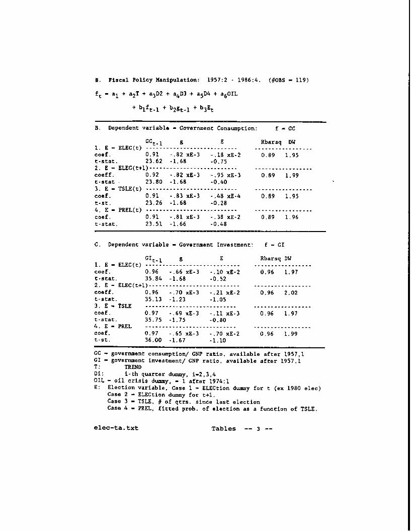
6. Piscal Policy Manipulation: 1957:2 - 1986:4. (908s — 119)

—a1 + a2T + a3D2 + a4D3 + a5D4 + a6OtL

+ bif,i ÷ b2g1, + b3E

B. Dependent variable — Government Consumption: f — CC

CC1 g E Rbarsq DW1. E — ELEC(t)coef. 0.91 -.82 xE-3 - .18 xE-2 0.89 1.95t-stat. 23.62 -1.66 -0.752. E — ELEC(t+1)coeff. 0.92 -.82 xE-3 - .95 xE-3 0.89 1.99t-stat 23.80 -1.68 -0.403. E — TSLE(t)coef. 0.91 - .83 xE-3 - .48 xE-4 0.89 1.95t-st. 23.26 -1.68 -0.284. E — PREL(t)coef. 0.91 - .81 xE-3 - .38 xE-2 0,89 1.96t-stat. 23.51 -1.66 -0.48

C. Dependent variable — Government Investment: — CI

GI1 g 8 Rbarsq OW1. E — ELEC(t)cod. 0.96 -.66 xE-3 -.10 xE-2 0.96 1.97t-stat. 35.84 -1.68 -0.522. E — ELEC(t+1)coeff. 0.96 - .70 xE-3 -.21 xE-2 0.96 2.02t-stat. 35.13 -1.23 -1.053. 8 — TSLEcoef. 0.97 - .69 xE-3 - .11 xE-3 0.96 1.97t-stat. 35.75 -1.75 -0.804. 8 — PRELcoef. 0.97 - .65 xE-3 - .70 xE-2 0.96 1.99t-st. 36.00 -1.67 -1.10

CC — government consumption! GNP ratio, available after 1957,1CI — government investment/ CNP ratio, available after 1957,1

TRENDDi: i-tb quarter dummy, i—2,3,4OIL — oil crisis dummy, — 1 after 1974:1E: Election variable, Case 1 — ELECtion dummy for t (cx 1980 dcc)

Case 2 — ELECtion dummy for t+l.Case 3 — TSLE, # of qtrs. since last electionCase 4 — PREL, fitted prob. of election as a function of ISLE.

elec—ta.txt Tables —— 3 —-

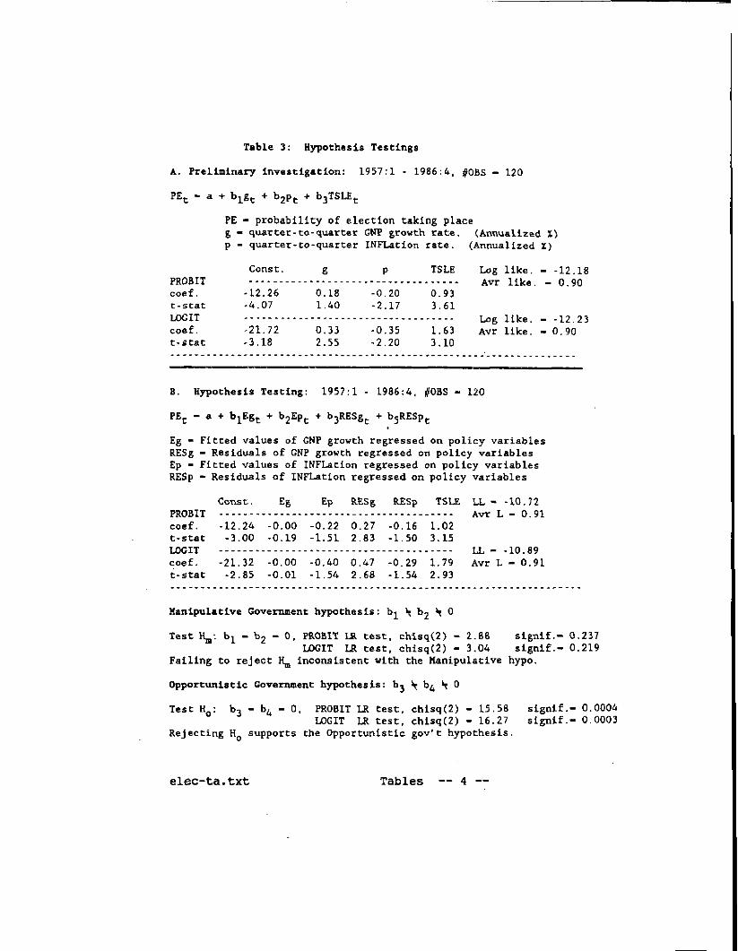
Table 3: Ky-pothesis Testings

A. Preliminary investigation: 1957:1 - 1986:4 #OBS — 120

PEt - a + b1g + b2p + bsTSLE

FE — probability of election taking place8 — quaxter-to-suarter fliP growth rate. (Annualized %)p — quarter-to-quarter INFLation rate. (Annualized 1)

Const. g p ISLE Log like. — -12.18PR03IT Avr like. — 0.90coef. -1.2.26 0.18 -0.20 0.93t-stat -4.07 1.40 -2.17 3.61LOGIT Log like. — -1223cooL -21.72 0.33 -0.35 1.63 Avr like. — 0.90t-stat -3.18 2.55 -2.20 3.10

a. Hypothesis Testing: 1957:1 - 1.986:4, #085 — 120

PE — a + b1Eg + b2Ep + b3RESg + bsRESpt

Eg — Fitted values of fliP growth regressed on policy variablesItESg — Residuals of ON? growth regressed on poLicy variablesEp — Fitted values of INFLation regressed on policy variablesRESp — Residuals of INFLation regressed on policy variables

Cotst. Eg Ep RES8 RESp TSLE LI.. — -10.72FROBIT Avr L — 0.91coef. -12.24 -0.00 -0.22 0.27 -0.16 1.02t-stat -3.00 -0.19 -1.51 2.83 -1.50 3.15LOGIT LI — -10.89coef. -21.32 -0,00 -0.40 0.47 -0.29 1.79 Avr L — 0.91t-stat -2.85 -0.01 -1.54 2.68 -1.54 2.93

Manipulative Government hypothesis: b1 ' 0

Test R: b1 — b2 — 0, PROM! LR test. chisq(2) — 1.88 stgnif.— 0.237LOGIT 11 test, chisq(2) — 3.04 signif.— 0.219

Failing to reject H inconsistent with the Manipulative hypo.

Opportunistic Government hypothes is: b3 b4 0

Test H0: b3 — b4 — 0, PROBIT LR test, chisq(2) — 15.58 signif.— 0.0004LOGIT IR test, chisq(2) — 16.27 signif.— 0.0003

Rejecting H0 supports the Opportunistic gov't hypothesis.

elec—ta.txt Tables —— 4 -—

: E1ecfon a5cks

0

5EOHf OIL CHISIS

71nLast

(QiQs)

JP3nsk ra(%)1o

a

6.

L

2.

-2

2 2 3 9 5 6 7 8 310111213 19 15 16

10

8

B

4-f

2

0.

-2

-96 9 10 11 12 13 19 15 16

Lcf

fl3&r€ 2. Eiec+;0 cd€AFTER OIL CRISIS

I 2 3 9 5 5 7