massive mimo has unlimited capacity - arxiv.org e … (icc), 21–25 may, 2017, paris, france....
TRANSCRIPT

1
Massive MIMO Has Unlimited CapacityEmil Bjornson, Member, IEEE, Jakob Hoydis, Member, IEEE, Luca Sanguinetti, Senior Member, IEEE
Abstract—The capacity of cellular networks can be improvedby the unprecedented array gain and spatial multiplexing offeredby Massive MIMO. Since its inception, the coherent interferencecaused by pilot contamination has been believed to create afinite capacity limit, as the number of antennas goes to infinity.In this paper, we prove that this is incorrect and an artifactfrom using simplistic channel models and suboptimal precod-ing/combining schemes. We show that with multicell MMSEprecoding/combining and a tiny amount of spatial channel corre-lation or large-scale fading variations over the array, the capacityincreases without bound as the number of antennas increases,even under pilot contamination. More precisely, the result holdswhen the channel covariance matrices of the contaminating usersare asymptotically linearly independent, which is generally thecase. If also the diagonals of the covariance matrices are linearlyindependent, it is sufficient to know these diagonals (and notthe full covariance matrices) to achieve an unlimited asymptoticcapacity.
Index Terms—Massive MIMO, ergodic capacity, asymptoticanalysis, spatial correlation, multi-cell MMSE processing, pilotcontamination.
I. INTRODUCTION
The Shannon capacity of a channel manifests the spectral ef-ficiency (SE) that it supports. Massive MIMO (multiple-inputmultiple-output) improves the sum SE of cellular networksby spatial multiplexing of a large number of user equipments(UEs) per cell [1]. It is therefore considered a key time-division duplex (TDD) technology for the next generationof cellular networks [2]–[4]. The main difference betweenMassive MIMO and classical multiuser MIMO is the largenumber of antennas, M , at each base station (BS) whosesignals are processed by individual radio-frequency chains. Byexploiting channel estimates for coherent receive combining,the uplink signal power of a desired UE is reinforced bya factor M , while the power of the noise and independentinterference does not increase. The same principle holds forthe transmit precoding in the downlink. Since the channel
c©2017 IEEE. Personal use of this material is permitted. Permission fromIEEE must be obtained for all other uses, in any current or future media,including reprinting/republishing this material for advertising or promotionalpurposes, creating new collective works, for resale or redistribution to serversor lists, or reuse of any copyrighted component of this work in other works.
E. Bjornson is with the Department of Electrical Engineering (ISY),Linkoping University, 58183 Linkoping, Sweden ([email protected]).J. Hoydis is with Nokia Bell Labs, Paris-Saclay, 91620 Nozay, France([email protected]). L. Sanguinetti is with the Universityof Pisa, Dipartimento di Ingegneria dell’Informazione, 56122 Pisa Italy([email protected]) and also with the Large Systems and NetworksGroup (LANEAS), CentraleSupelec, Universite Paris-Saclay, 3 rue Joliot-Curie, 91192 Gif-sur-Yvette, France. The authors have contributed equallyto this work and are listed alphabetically.
This research has been supported by ELLIIT, the Swedish Foundation forStrategic Research (SFF), the EU FP7 under ICT-619086 (MAMMOET), andthe ERC Starting Grant 305123 MORE.
Parts of this paper were presented at the International Conference onCommunications (ICC), 21–25 May, 2017, Paris, France.
estimates are obtained by uplink pilot signaling and the pilotresources are limited by the channel coherence time, thesame pilots must be reused in multiple cells. This leads topilot contamination which has two main consequences: thechannel estimation quality is reduced due to pilot interferenceand the channel estimate of a desired UE is correlated withthe channels to the interfering UEs that use the same pilot.Marzetta showed in his seminal paper [1] that the interferencefrom these UEs during data transmission is also reinforcedby a factor M , under the assumptions of maximum ratio(MR) combining/precoding and independent and identicallydistributed (i.i.d.) Rayleigh fading channels. This means thatpilot contamination creates a finite SE limit as M →∞.
The large-antenna limit has also been studied for othercombining/precoding schemes, such as the minimum meansquared error (MMSE) scheme. Single-cell MMSE (S-MMSE)was considered in [5]–[7], while multicell MMSE (M-MMSE)was considered in [8], [9]. The difference is that with M-MMSE, the BS makes use of estimates of the channels fromthe UEs in all cells, while with S-MMSE, the BS only useschannel estimates of the UEs in the own cell. In both cases,the SE was proved to have a finite limit as M →∞, under theassumption of i.i.d. Rayleigh fading channels (i.e., no spatialcorrelation). In contrast, there are special cases of spatiallycorrelated fading that give rise to rank-deficient covariancematrices [10]–[12]. If the UEs that share a pilot have rank-deficient covariance matrices with orthogonal support, thenpilot contamination vanishes and the SE can increase withoutbound. The covariance matrices R1 and R2 have orthogonalsupport if R1R2 = 0. To understand this condition, note thatfor arbitrary covariance matrices
R1 =
[a cc? b
]R2 =
[d ff? e
](1)
every element of R1R2 must be zero. The first element isad + cf?. If we model the practical covariance matrices oftwo randomly located UEs as realizations of a random variablewith continuous distribution, then ad + cf? = 0 occurs withzero probability.1 Hence, orthogonal support is very unlikelyin practice, although one can find special cases where it issatisfied. The one-ring model for uniform linear arrays (ULAs)gives orthogonal support if the channels have non-overlappingangular support [10]–[12], but the ULA microwave measure-ments in [13] show that the angular support of practicalchannels is highly irregular and does not lead to orthogonalsupport. In conclusion, practical covariance matrices do nothave orthogonal support, at least not at microwave frequencies.
1For any continuous random variable x, the probability that x takes aparticular realization is zero, while the probability that x takes a realizationin a certain interval can be non-zero. Hence, if x = ad + cf? then x = 0occurs with zero probability.
arX
iv:1
705.
0053
8v4
[cs
.IT
] 9
Nov
201
7
2
The literature contains several categories of methods formitigation of pilot contamination, also known as pilot decon-tamination. The first category allocates pilots to the UEs in anattempt to find combinations where the covariance matriceshave relatively different support [10]–[12], [14]. This methodcan substantially reduce pilot contamination, but can onlyremove the finite limit in the unlikely special case when thecovariance matrices have orthogonal support. The second cate-gory utilizes semi-blind estimation to separate the subspace ofdesired UE channels from the subspace of interfering channels[15]–[19]. This method can fully remove pilot contaminationif M and the size of the channel coherence block go jointly toinfinity [18]. Unfortunately, the channel coherence is fixed andfinite in practice (this is why we cannot give unique pilots toevery cell), thus we cannot approach this limit in practice. Thethird category uses multiple pilot phases with different pilotsequences to successively eliminate pilot contamination [20],[21], without the need for statistical information. However, thetotal pilot length is larger or equal to the total number of UEs,which would allow allocating mutually orthogonal pilots to allUEs and thus trivially avoiding the pilot contamination prob-lem. This is not a scalable solution for networks with manycells. The fourth category is pilot contamination precoding thatrejects interference by coherent joint transmission/receptionover the entire network [22], [23]. This method appears toachieve an unbounded SE, but this has not been formallyproved and requires that the data for all UEs is available atevery BS, which might not be feasible in practice.
In summary, it appears that pilot contamination is a funda-mental issue that manifests a finite SE limit, except in unlikelyspecial cases. We show in this paper that this is basicallya misunderstanding, spurred by the popularity of analyzingsuboptimal combining/precoding schemes, such as MR andS-MMSE, and focusing on unrealistic i.i.d. Rayleigh fadingchannels (as in the prior work [8], [9] on M-MMSE). We provethat the SE increases without bound in the presence of pilotcontamination when using M-MMSE combining/precoding, ifthe pilot-sharing UEs have asymptotically linearly indepen-dent covariance matrices. Note that R1 and R2 in (1) arelinearly independent if [a b c]T and [d e f ]T are non-parallelvectors, which happens almost surely for randomly generatedcovariance matrices. Hence, our results rely on a conditionthat is most likely satisfied in practice—it is the general case,while prior works on the asymptotics of Massive MIMO haveconsidered practically unlikely special cases. In contrast toprior work, no multicell cooperation is utilized herein andthere is no need for orthogonal support of covariance matrices.In the conference paper [24], we proved the main result in atwo-user uplink scenario.2 In this paper, we prove the resultfor both uplink and downlink in a general setting. Section IIproves and explains the intuition of the results in a two-usersetup, while Section III generalizes the results to a multicell
2After submitting our conference paper [24], the related work [25] appeared.That paper considers the mean squared error in the uplink data detection of asingle cell with multiple UEs per pilot sequence. The authors show that theerror goes asymptotically to zero when having linearly independent covariancematrices. However, the paper [25] contains no mathematical analysis of theachievable SE.
setup. The results are demonstrated numerically in Section IVand the main conclusions are summarized in Section V.
Notation: The Frobenius and spectral norms of a matrix Xare denoted by ‖X‖F and ‖X‖2, respectively. The superscriptsT, ? and H denote transpose, conjugate, and Hermitian trans-pose, respectively. We use , to denote definitions, whereasNC(0,R) denotes the circularly symmetric complex Gaussiandistribution with zero mean and covariance matrix R. Theexpected value of a random variable x is denoted by E{x}and the variance is denoted by V{x}. The N × N identitymatrix is denoted by IN , while 0N is an N × N all-zeromatrix and 1N is an N × 1 all-one vector. We use an � bnto denote an − bn →n→∞ 0 (almost surely (a.s.)) for two(random) sequences an, bn.
II. ASYMPTOTIC SPECTRAL EFFICIENCY IN A TWO-USERSCENARIO
In this section, we prove and explain our main result ina two-user scenario, where a BS equipped with M antennascommunicates with UE 1 and UE 2 that are using the samepilot. This setup is sufficient to demonstrate why M-MMSEcombining and precoding reject the coherent interferencecaused by pilot contamination. We consider a block-fadingmodel where each channel takes one realization in a coherenceblock of τc channel uses and independent realizations acrossblocks. We denote by hk ∈ CM the channel from UE k to theBS and consider Rayleigh fading with hk ∼ NC (0,Rk) fork = 1, 2, where Rk ∈ CM×M with3 tr(Rk) > 0 is the chan-nel covariance matrix, which is assumed to be known at theBS. The Gaussian distribution models the small-scale fadingwhereas the covariance matrix Rk describes the macroscopiceffects. The normalized trace βk = 1
M tr (Rk) determines theaverage large-scale fading between UE k and the BS, while theeigenstructure of Rk describes the spatial channel correlation.A special case that is convenient for analysis is i.i.d. Rayleighfading with Rk = βkIM [26], but it only arises in fullyisotropic fading environments. In general, each covariancematrix has spatial correlation and large-scale fading variationsover the array, represented by non-zero off-diagonal elementsand non-identical diagonal elements, respectively.
A. Uplink Channel Estimation
We assume that the BS and UEs are perfectly synchronizedand operate according to a TDD protocol wherein the datatransmission phase is preceded by an uplink pilot phase forchannel estimation. Both UEs use the same τp-length pilotsequence φ ∈ Cτp with elements such that ‖φ‖2 = φHφ = 1.The received uplink signal Yp ∈ CN×τp at the BS is givenby
Yp =√ρtrh1φ
T +√ρtrh2φ
T + Np (2)
where ρtr is the normalized pilot power and Np ∈ CN×τp isthe normalized receiver noise with all elements independentlydistributed as NC(0, 1). The matrix Yp is the observation that
3This assumption implies that there is non-zero energy received from andtransmitted to each UE.

3
the BS utilizes to estimate h1 and h2. We assume that channelestimation is performed using the MMSE estimator given inthe next lemma (the proof relies on standard estimation theory[27]).
Lemma 1. The MMSE estimator of hk for k = 1, 2, basedon the observation Yp at the BS, is
hk =1√ρtr
RkQ−1Ypφ? (3)
with Q = 1ρtrE{Y
pφ?(Ypφ?)H} = R1 + R2 + 1ρtr IM
being the normalized covariance matrix of the observationafter correlating with the pilot sequence. The estimate hkand the estimation error hk = hk − hk are independentrandom vectors distributed as hk ∼ NC(0,Φk) and hk ∼NC(0,Rk −Φk) with Φk = RkQ
−1Rk.
Interestingly, the estimates h1 and h2 are computed in analmost identical way in (3): the same matrix Q is inverted andmultiplied with the same observation Ypφ?/
√ρtr. The only
difference is that for hk there is a multiplication with the UE’sown channel covariance matrix Rk in (3), for k = 1, 2. Thechannel estimates are thus correlated with correlation matrixΥ12 = E{h1h
H2} = R1Q
−1R2. If R1 is invertible, then wecan also write the relation between the estimates as h2 =R2R
−11 h1. In the special case of i.i.d. fading channels with
R1 = β1IM and R2 = β2IM , the two channel estimates areparallel vectors that only differ in scaling: h2 = β2
β1h1. This
is an unwanted property caused by the inability of the BS toseparate UEs that have transmitted the same pilot sequenceover channels that are identically distributed (up to a scalingfactor). In the alternative special case of R1R2 = 0M , the twoUE channels are located in orthogonal subspaces (i.e., haveorthogonal support), which leads to zero correlation: Υ12 =0M . Consequently, it is theoretically possible to let two UEsshare a pilot sequence without causing pilot contamination, iftheir covariance matrices satisfy the orthogonality conditionR1R2 = 0M . As described in Section I, none of these specialcases occur in practice, therefore we will develop a generalway to deal with the correlation of channel estimates causedby pilot contamination.
B. Uplink Data Transmission
During uplink data transmission, the received basebandsignal at the BS is y ∈ CM , given by y =
√ρulh1s1 +√
ρulh2s2 + n, where sk ∼ NC(0, 1) is the information-bearing signal transmitted by UE k, n ∼ NC(0, IM ) is theindependent receiver noise, and ρul is the normalized transmitpower. The BS detects the signal from UE 1 by using acombining vector v1 ∈ CM to obtain vH
1 y. Using a standardtechnique (see, e.g., [5], [26]), the ergodic uplink capacity ofUE 1 is lower bounded by
SEul1 =
(1− τp
τc
)E{
log2
(1 + γul
1
)}[bit/s/Hz] (4)
where the expectation is with respect to the channel estimates.We refer to SEul
1 as an achievable SE. The instantaneouseffective signal-to-interference-and-noise ratio (SINR) γul
1 in(4) is
γul1 =
|vH1 h1|2
E{|vH
1 h1|2 + |vH1 h2|2 + 1
ρulvH
1 v1
∣∣∣h1, h2
}=
|vH1 h1|2
vH1
(h2hH
2 + Z)
v1
(5)
with Z =∑2k=1(Rk−Φk)+ 1
ρulIM . Since γul
1 is a generalizedRayleigh quotient, the SINR is maximized by [8], [9]
v1 =
(2∑k=1
hkhH
k + Z
)−1
h1. (6)
This is called MMSE combining since (6) not only maximizesthe instantaneous SINR γul
1 , but also minimizes E{|x1 −vH
1 y|2 |h1, h2} which is the mean squared error (MSE) inthe data detection (conditioned on the channel estimates).Plugging (6) into (5) yields
γul1 = hH
1
(h2h
H
2 + Z)−1
h1. (7)
We will now analyze the asymptotic behavior of SEul1 and γul
1
as M → ∞. To this end, we make the following technicalassumptions:
Assumption 1. For k = 1, 2, lim infM
1M tr(Rk) > 0 and
lim supM
‖Rk‖2 <∞.
Assumption 2. For λ = [λ1, λ2]T ∈ R2 and i = 1, 2,
lim infM
inf{λ:λi=1}
1
M‖λ1R1 + λ2R2‖2F > 0. (8)
The first assumption is a well established way to model thatthe array gathers more energy as M increases and also thatthis energy originates from many spatial dimensions [5]. Inparticular, it is a sufficient condition for asymptotic channelhardening; that is, ‖hk‖2/E{‖hk‖2} → 1 in probability asM → ∞. The second assumption requires R1 and R2 tobe asymptotically linearly independent, in the sense that ifone of the matrices is scaled to resemble the other one, thesubspace in which the matrices differ has an energy propor-tional to M . Note that this is a stronger condition than linearindependence, defined as inf{λ:λi=1} ‖λ1R1 + λ2R2‖2F > 0for i = 1, 2, which is satisfied even if the matrices only differin one element. We will elaborate further on Assumption 2 inSection II-D.
The following is the first of the main results of this paper:
Theorem 1. If MMSE combining is used, then under As-sumptions 1 and 2, the instantaneous effective SINR γul
1
increases a.s. unboundedly as M →∞. Hence, SEul1 increases
unboundedly as M →∞.
Proof: The proof is given in Appendix B.
Remark 1. From the proof in Appendix B, we can see thatγul
1 /M has a non-zero asymptotic limit, which implies that theSE grows towards infinity as log2(M). While Theorem 1 onlyconsiders UE 1, one only needs to interchange the UE indicesto prove that the SE of UE 2 also grows unboundedly as

4
M →∞. Hence, an unlimited asymptotic SE is simultaneouslyachievable for both UEs. Since the SE is a lower bound oncapacity, we conclude that the asymptotic capacity is alsounlimited.
Observe that if R1 and R2 are linearly dependent, i.e.,R1 = ηR2, then Assumption 2 does not hold. Under thesecircumstances, h2 = 1
η h1 and by applying Lemma 5 inAppendix A we obtain
γul1 =
hH1 Z−1h1
1 + 1η2 hH
1 Z−1h1
(9)
from which, it is straightforward to show that γul1 � η2 (by
dividing and multiplying each term by M and using Lemma 3in Appendix A). This implies that SEul
1 converges to a finitequantity when M → ∞, as Marzetta showed in his seminalpaper [1] for the special case of R1 = ηR2 = IM .
C. Downlink Data Transmission
During the downlink data transmission, the BS transmitsthe signal x ∈ CM . This signal is given by x =
√ρdlw1ς1 +√
ρdlw2ς2, where ςk ∼ NC(0, 1) is the information-bearingsignal transmitted to UE k, ρdl is the normalized downlinktransmit power, and wk is the precoding vector associatedwith UE k. This precoding vector satisfies E
{‖wk‖2
}= 1,
so that E{‖wkςk‖2
}= ρdl is the downlink transmit power
allocated to UE k. The received downlink signal z1 at UE 1is4
z1 =√ρdlhH
1 w1ς1 +√ρdlhH
1 w2ς2 + n1
=√ρdlE {hH
1 w1} ς1 +√ρdl(hH
1 w1 − E {hH
1 w1})ς1+√ρdlhH
1 w2ς2 + n1 (10)
where n1 ∼ NC(0, 1) is the normalized receiver noise. Thefirst term in (10) is the desired signal received over thedeterministic average precoded channel E {hH
1 w1}, while theremaining terms are random variables with unknown realiza-tions. By treating these terms as noise in the signal detection[5], [26], the downlink ergodic channel capacity of UE 1 canbe lower bounded by
SEdl1 =
(1− τp
τc
)log2
(1 + γdl
1
)[bit/s/Hz] (11)
with the effective SINR
γdl1 =
|E{hH1 w1}|2
E {|hH1 w2|2}+ V {hH
1 w1}+ 1ρdl
. (12)
Since UE 1 only needs to know E {hH1 w1} and the total
variance of the second to fourth term in (10), the SE in (11)is achievable in the absence of downlink channel estimation.In contrast to the uplink, there is no precoding that is alwaysoptimal [28]. However, motivated by uplink-downlink duality
4For notational convenience, we treat hH1 and hH
2 as the downlink channels,instead of hT
1 and hT2 . This has no impact on the SE since the difference is
only in a complex conjugate.
[9], a reasonable suboptimal choice is the so-called MMSEprecoding
wk =vk√
E {‖vk‖2}=√ϑk
(2∑k=1
hkhH
k + Z
)−1
hk (13)
where vk = (∑2k=1 hkh
H
k+Z)−1hk is MMSE combining andϑk = (E
{‖vk‖2
})−1 is a scaling factor. The following is the
second main result of this paper:
Theorem 2. If MMSE precoding is used, then under Assump-tions 1 and 2 the effective SINR γdl
1 increases unboundedly asM →∞. Hence, SEdl
1 increases unboundedly as M →∞.
Proof: The proof is given in Appendix D.This theorem shows that, under the same conditions as in
the uplink, the downlink SE (and thus the capacity) increaseswithout bound as M → ∞. The asymptotic SE growthis proportional to log2(M), since the proof in Appendix Dshows that γdl
1 /M has a non-zero asymptotic limit. UE 2 cansimultaneously achieve an unbounded SE, which is proveddirectly by interchanging the UE indices.
D. Interpretation and Generality
Theorems 1 and 2 show that the SE (and thus the capac-ity) under pilot contamination is asymptotically unlimited ifAssumption 2 holds. To gain an intuitive interpretation ofthis underlying assumption, recall from (3) that h1 = R1aand h2 = R2a, where a = 1√
ρtrQ−1Ypφ∗ is the same
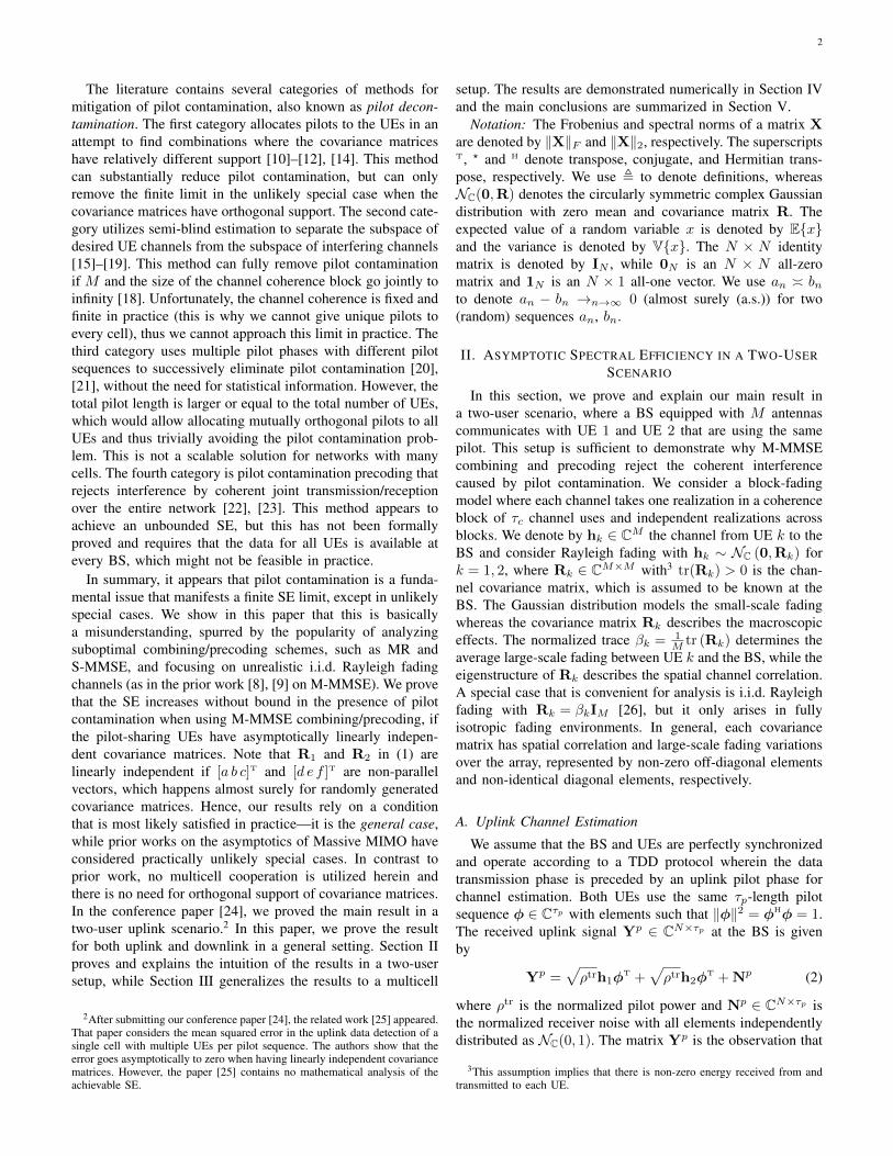
for both UEs. Hence, h1 and h2 are (asymptotically) linearlyindependent when R1 and R2 are (asymptotically) linearlyindependent, except for special choices of a. As illustrated inFig. 1, it is then possible to find a combining vector v1 (orprecoding vector w1) that is orthogonal to h2, while beingnon-orthogonal to h1. Similarly, one can find v2 (and w2)such that vH
2 h1 = 0 and vH2 h2 6= 0. For example, if we define
H = [h1 h2] ∈ CM×2, then the zero-forcing (ZF) combiningvectors [
v1 v2
]= H
(HHH
)−1
(14)
satisfy these conditions. Note that HHH is only invertible ifthe channel estimates (columns in H) are linearly independent.Using ZF as defined in (14), we get vH
1 h2 = 0 and vH1 h1 =
1. If the channel estimates are also asymptotically linearlyindependent, it follows5 that ‖v1‖2 → 0 as M → ∞; thatis, we can reject the coherent interference and get unit signalgain, while at the same time using the array gain to makethe noise term 1
ρulvH
1 v1 = 1ρul‖v1‖2 vanish asymptotically.
Since optimal MMSE combining (and also MMSE precoding)provides a higher SINR than the heuristic ZF scheme in (14),it also rejects the coherent interference while retaining an arraygain that grows with M .
To further explain the implications of Assumption 2, weprovide the following three examples.
5Notice that, by applying Lemma 3 in Appendix A, we have1M
[HHH]nm � 1M
tr(RnQ−1Rm). If the channel estimates are asymp-totically linearly independent, then 1
MHHH is invertible as M → ∞ and
thus ‖v1‖2 = 1M
[( 1M
HHH)−1]11 � 0.
5
h1
h2
Orthogonal only to h2
v1
Fig. 1: If the pilot-contaminated channel estimates are linearlyindependent (i.e., not parallel), there exists a combining vector v1 thatrejects the pilot-contaminated interference from UE 2 in the uplink,while the desired signal remains due to vH
1 h1 6= 0. Similarly, ifw1 = v1/
√E{‖v1‖2} is used as precoding vector, then no pilot-
contaminated coherent interference is caused to UE 2 in the downlink.
Example 1. Consider a two-user scenario with
R1 =
[2IN 00 IM−N
]R2 = IM (15)
where the covariance matrices have full rank and are onlydifferent in the first N dimensions. For any given M , we noticethat the argument of (8) for UE i = 1 becomes
infλ2
1
M‖R1 + λ2R2‖2F
= infλ2
N(2 + λ2)2 + (M −N)(1 + λ2)2
M=
(M −N)N
M2
(16)
where the infimum is attained by λ2 = −(M + N)/M .Note that (16) goes to zero as M → ∞ if N is constant,while it has the non-zero limit (1 − α)α if N = αM ,for some 0 < α < 1. In the latter case, the matrices{R1,R2} satisfy (8). Interestingly, although the covariancematrices are diagonal, they are still asymptotically linearlyindependent and the subspace in which they differ has rankmin(N,M −N) = M min(α, (1−α)), which is proportionalto M .
Let us further exemplify the interference rejection by consid-ering ZF combining, which provides lower SINR than MMSEcombining, but gives more intuitive expressions. Assume forthe sake of simplicity that the channel realizations are suchthat 1√
ρtrQ−1Ypφ∗ = 1M , which gives h1 = R11M =
[21T
N 1T
M−N ]T and h2 = R21M = 1M . The ZF combiningvectors are then given by[
v1 v2
]= H
(HHH
)−1
=
[1N 1N − 1
N 1N− 1M−N 1M−N 2
M−N 1M−N
].
(17)If we set ρul = ρul = 1 for simplicity, the instantaneouseffective SINR in (5) for UE 1 becomes
γul1 =
|vH1 h1|2
|vH1 h2|2 +
∑2k=1 vH
1 (Rk −Φk)v1 + ‖v1‖2
=1
0 + 74N + 4
3(M−N) + MN(M−N)
(18)
where the coherent interference from UE 2 is zero. Theremaining terms go asymptotically to zero if N = αM , for0 < α < 1, in which case γul
1 grows without bound, asexpected from Theorem 1.
In the second example, we consider a scenario whereAssumption 2 is not satisfied.
Example 2. Channels with i.i.d. fading, where the covariancematrices are R1 = β1IM and R2 = β2IM , are a notable casewhen the covariance matrices are not linearly independent.However, any such case is non-robust to perturbations of thematrix elements. Suppose we replace R1 with
R1 = β1
ε1 0 · · ·
0. . . 0
... 0 εM
(19)
where ε1, . . . , εM are i.i.d. positive random variables. Thismodeling is motivated by the measurement results in [29],which shows that there are a few dB of large-scale fadingvariations over the antennas in a ULA. For UE i = 1, wehave
lim infM
infλ2
1
M‖R1 + λ2R2‖2F
= lim infM
infλ2
1
M
M∑m=1
(β1εm + λ2β2)2
(a)= lim inf
Mβ2
1
1
M
M∑m=1
(εm −
1
M
M∑n=1
εn
)2
(b)= β2
1E{(εm − E{εm})2} (20)
where (a) is obtained from the fact that λ2 = −β1
β2
1M
∑Mn=1 εn
minimizes 1M
∑Mm=1(β1εm +λ2β2)2 and (b) follows from the
strong law of large numbers. Note that E{(εm−E{εm})2} inthe last expression is the variance of εm. Since every randomvariable has non-zero variance and β1 > 0, we conclude that{R1,R2} satisfy (8) and thus Assumption 2 holds.
The key implication from Example 2 is that all cases whereR1 and R2 are equal (up to a scaling factor) are non-robustto random perturbations and thus anomalies. Since practicalpropagation environments are irregular and behave randomly(see the measurements reported in [13], [29]), linearly depen-dent covariance matrices are not appearing in practice andAssumption 2 is generally satisfied. In other words, it is fairto say that the uplink and downlink SEs grow without bound asM →∞ in general, while the special cases when it does notoccur are of no practical importance. We end this subsectionwith a comparison with related work and a remark regardingacquisition of channel statistics.
Example 3 (Comparison with [22], [23]). Consider a BS withtwo distributed arrays of M ′ = M/2 antennas that serve twoUEs having the covariance matrices
R1 =
[b11IM ′ 0
0 b12IM ′
]R2 =
[b21IM ′ 0
0 b22IM ′
](21)
with b11, b12, b21, b22 > 0. These covariance matrices are(asymptotically) linearly independent if b11b22 6= b12b21, inwhich case the uplink and downlink SEs grow without boundwith MMSE or ZF.
6
The exemplified setup is equivalent to the multicell jointtransmission scenario considered in the pilot contaminationprecoding works [22], [23] in which the heuristic vectors[
v1 v2
]=
[1M ′y
p1 0
0 1M ′y
p2
] [b11 b12
b21 b22
]−1
(22)
are used for combining and precoding, and yp1,yp2 ∈ CM ′ are
obtained from the received pilot signals as [(yp1)T (yp2)T]T =Ypφ?/ρtr. These vectors are specifically designed to make[h1 h2
]H[v1 v2
]� I2 as M → ∞, and thus this method
has the same asymptotic behavior as ZF in the special caseof block-diagonal covariance matrices where each block is ascaled identity matrix. Note that the matrix inverse in (22)only exists if b11b22 6= b12b21, which is again the conditionfor linear independence of the covariance matrices. Sincepilot contamination precoding can only be applied in specialmulticell cooperation cases, MMSE combining/precoding isgenerally the preferable choice.
Remark 2 (Acquiring Covariance Matrices). Theorems 1 and2 exploit the MMSE estimator and thus the BS needs to knowthe (deterministic) channel statistics. In particular, the BS canonly compute the MMSE estimate hk in Lemma 1 if it knowsRk and also the sum R1 +R2 of the two covariance matrices.In practice, Rk can be estimated by a regularized samplecovariance matrix, given realizations of hk over multipleresource blocks (e.g., different times and frequencies) wherethis channel is either observed in only noise [10], [30], [31]or where some observations are regular pilot transmissionscontaining the desired channel plus interference/noise andsome contain only the interference/noise [32]. It seems thataround M samples are needed to obtain a sufficiently accuratecovariance estimate [32]. The covariance estimation can befurther improved if the channels have a known structure.For example, [33] provides algorithms for estimating thecovariance matrices of channels that have limited angle-delaysupport that is also separable between users.
E. Achievable SE with Partial Knowledge of Covariance Ma-trices
If the BS does not have full knowledge of the covariancematrices, an alternative method for channel estimation is toestimate each entry of hk separately, ignoring the correlationamong the elements. This leads to the element-wise MMSE(EW-MMSE) estimator (called diagonalized estimator in [30])that utilizes only the main diagonals of R1 and R2. Thediagonals can be estimated efficiently using a small numberof samples, that does not need to grow with M [30], [32].
Lemma 2. Based on the observation [Ypφ∗]i, the BS cancompute the EW-MMSE estimate of the ith element of hk as
[hk]i =1√ρtr
[Rk]ii
[R1]ii + [R2]ii + 1ρtr
[Ypφ∗]i. (23)
We may write hk in Lemma 2 in matrix form as
hk =1√ρtr
DkΛ−1Ypφ∗ (24)
where Dk ∈ RM×M and Λ ∈ RM×M are diagonal matriceswith elements {[Rk]ii : i = 1, . . . ,M} and {[R1]ii+[R2]ii+1ρtr : i = 1, . . . ,M}, respectively. Notice that Assumption 1implies that6 lim infM
1M tr(Dk) > 0 and lim supM ‖Dk‖2 <
∞ for k = 1, 2. To quantify the achievable SE when usingEW-MMSE, similar to the downlink we exploit the use-and-then-forget SE bound [26], which is less tight than (4) butdoes not require the use of MMSE channel estimation. Theuplink ergodic capacity of UE 1 can be thus lower boundedby SEul
1 = (1− τpτc
) log2(1 + γul1
) [bit/s/Hz] with
γul1
=|E{vH
1 h1}|2
E {|vH1 h2|2}+ V{vH
1 h1}+ 1ρul
E {‖v1‖2}. (25)
This bound is valid for any channel estimation and any com-bining scheme. A reasonable choice for v1 is the approximateMMSE combining vector:
v1 =
( 2∑k=1
hkhH
k + S
)−1
h1 (26)
where h1, h2 are computed as in (24) and S is diagonal andgiven by S =
∑2k=1
(Dk −DkΛ
−1Dk
)+ 1
ρulIM . Note that
(26) is equivalent to the MMSE combining in (6) when thecovariance matrices are diagonal. We will now analyze howγul
1behaves asymptotically as M →∞ when v1 is given by
(26). To this end, we impose the following assumption, whichstates that D1 and D2 are asymptotically linearly independent(i.e., the diagonals of R1 and R2 are asymptotically linearlyindependent).
Assumption 3. For λ = [λ1, λ2]T ∈ R2 and i = 1, 2,
lim infM
inf{λ:λi=1}
1
M‖λ1D1 + λ2D2‖2F > 0. (27)
The following is the third main result of this paper:
Theorem 3. If v1 in (26) is used with h1, h2 given by (24),then under Assumptions 1 and 3, the SINR γul
1increases
unboundedly as M →∞. Hence, SEul1 increases unboundedly
as M →∞.
Proof: The proof is given in Appendix E.As a consequence of this theorem, under Assumptions 1 and
3, the uplink SEs of UE 1 and UE 2 increase without bound asM → ∞ even if the BS has only knowledge of the diagonalelements of the covariance matrices. A similar result can beproved for the downlink, using the methodology adopted inAppendix D for proving Theorem 2. The details are omittedfor space limitations.
III. ASYMPTOTIC SPECTRAL EFFICIENCY IN MULTICELLMASSIVE MIMO
We will now generalize the results of Section II to a MassiveMIMO network with L cells, each comprising a BS with Mantennas and K UEs. There are τp = K pilots and the kth
6This easily follows by observing that tr(Rk) = tr(Dk) and also that[Dk]ii = [Rk]ii ≤ ‖Rk‖2 since Rk is Hermitian.
7
UE in each cell uses the same pilot. Following the notationfrom [5], the received signal yj ∈ CM at BS j is
yj =
L∑l=1
K∑i=1
√ρhjlixli + nj (28)
where ρ is the normalized transmit power, xli is the unit-power signal from UE i in cell l, hjli ∼ NC(0,Rjli) is thechannel from this UE to BS j, Rjli ∈ CM×M is the channelcovariance matrix, and nj ∼ NC(0, IM ) is the independentreceiver noise at BS j. Using a total uplink pilot power of ρtr
per UE and standard MMSE estimation techniques [5], BS jobtains the estimate of hjli as
hjli = RjliQ−1ji
( L∑l′=1
hjl′i +1√ρtr
nji
)∼NC (0,Φjli)
(29)
where nji ∼ NC(0, IM ) is noise, Qji =∑Ll′=1 Rjl′i+
1ρtr IM ,
and Φjli = RjliQ−1ji Rjli. The estimation error hjli = hjli−
hjli ∼ NC (0,Rjli −Φjli) is independent of hjli. However,the estimates hj1i, . . . , hjLi of the UEs with the same pilotare correlated as E{hjnihH
jmi} = RjniQ−1ji Rjmi.
A. Uplink Data Transmission
We denote by vjk ∈ CM the receive combining vectorassociated with UE k in cell j. Using the same techniqueas in [5], [26], the uplink ergodic capacity is lower boundedby
SEuljk =
(1− τp
τc
)E{
log2
(1 + γul
jk
)}[bit/s/Hz] (30)
with the instantaneous effective SINR
γuljk =
|vH
jkhjjk|2
E
{ ∑(l,i) 6=(j,k)
|vH
jkhjli|2 + |vH
jkhjjk|2 +vHjkvjk
ρul
∣∣∣h(j)
}
=|vH
jkhjjk|2
vH
jk
( ∑(l,i)6=(j,k)
hjlihH
jli + Zj
)vjk
(31)
where E{·|h(j)} denotes the conditional expectation giventhe MMSE channel estimates available at BS j and Zj =∑Ll=1
∑Ki=1(Rjli −Φjli) + 1
ρul IM . As shown in [8], [9], theinstantaneous effective SINR in (31) for UE k in cell j ismaximized by
vjk =
(L∑l=1
K∑i=1
hjlihH
jli + Zj
)−1
hjjk. (32)
We refer to this “optimal” receive combining scheme as mul-ticell MMSE (M-MMSE) combining. The “multicell” notionis used to differentiate it from the single-cell MMSE (S-MMSE) combining scheme [5]–[7], which is widely used inthe literature and defined as
vjk =
(K∑i=1
hjjihH
jji + Zj
)−1
hjjk (33)
with Zj =∑Ki=1 Rjji−Φjji +
∑Ll=1,l 6=j
∑Ki=1 Rjli + 1
ρulIM .
The main difference from (32) is that only channel estimatesin the own cell are computed in S-MMSE, while hjlih
H
jli −Φjli is replaced with its average (i.e., zero) for all l 6= j.The computational complexity of S-MMSE is thus slightlylower than with M-MMSE (see [9] for a detailed discussion).However, both schemes only utilizes channel estimates thatcan be computed locally at the BS and the pilot overhead isidentical since the same pilots are used to estimate both intra-cell and inter-cell channels. The S-MMSE scheme coincideswith M-MMSE when there is only one isolated cell, but itis generally different and does not suppress interference frominterfering UEs in other cells. Plugging (32) into (31) yields
γuljk = hH
jjk
( ∑(l,i) 6=(j,k)
hjlihH
jli + Zj
)−1
hjjk. (34)
We want to analyze γuljk when M →∞. To this end, we make
the following two assumptions.
Assumption 4. As M →∞ ∀j, l, i, lim infM1M tr(Rjli) > 0
and lim supM ‖Rjli‖2 <∞.
Assumption 5. For any UE k in cell j with λjk =[λj1k, . . . , λjLk]T ∈ RL and l′ = 1, . . . , L
lim infM
inf{λjk:λjl′k=1}
1
M
∥∥∥∥∥L∑l=1
λjlkRjlk
∥∥∥∥∥2
F
> 0. (35)
The following is the fourth main result of the paper:
Theorem 4. If M-MMSE combining is used, then underAssumptions 4 and 5 the SINR γul
jk increases a.s. unboundedlyas M →∞. Hence, SEul
jk increases unboundedly as M →∞.
Proof: The proof is given in Appendix F.This theorem proves the remarkable result that, under As-
sumptions 4 and 5, the uplink SE of a multicell MassiveMIMO network increases without bound as M →∞, despitepilot contamination. This is in sharp contrast to the finitelimit in case of MR combining [1] or any other single-cell combining scheme [5]–[7] and it is due to the fact thatM-MMSE rejects the coherent interference caused by pilotcontamination when Assumptions 4 and 5 hold. Note that theseare the natural multicell generalizations of Assumptions 1and 2, respectively. In particular, the condition (35) saysthat the covariance matrices {Rjlk : l = 1, . . . , L} of thechannels from the pilot-sharing UEs to BS j are asymptoticallylinearly independent, which implies the same condition forthe estimated channels {hjlk : l = 1, . . . , L}. This conditionis used in Appendix F to prove Theorem 4 in a fairlysimple way. However, we stress that Theorem 4 is valid alsoin a more general setting in which hjjk is asymptoticallylinearly independent of the estimates of all pilot-interferingUEs’ channels, but some of the interfering channel estimatescan be written as linear combinations of other interferingchannels. Let Sjk ⊆ {hjlk : ∀l 6= j} denote a subset ofthe estimated interfering channels that form a basis for allinterfering channels. Under these circumstances, we only needto take the estimates in Sjk into account in the computation of
8
the combining vector vjk in (32) and the same result follows.To gain further insights into this, we notice (as done for thetwo-user case in Section II-D) that one can find a receivecombining vector that is orthogonal to the subspace spannedby Sjk. This scheme exhibits an unbounded SE when M →∞as it rejects the interference from all pilot-contaminating UEs(not only from those in Sjk), while retaining an array gainthat grows with M . We call this scheme multicell ZF (M-ZF)and define it as vjk = Hjk
(HH
jkHjk
)−1e1, where e1 is the
first column of I|Sjk|+1 (with |Sjk| being the cardinality ofSjk) and Hjk ∈ CN×(|Sjk|+1) is the matrix with hjjk in thefirst column and the channel estimates in Sjk in the remainingcolumns. Since M-MMSE combining is the optimal scheme, ithas to exhibit an unbounded SE if this is the case with M-ZF.
B. Downlink Data Transmission
During downlink data transmission, the BS in cell l trans-mits xl =
√ρdl∑Kl=1 wliςli, where ςli ∼ NC(0, 1) is the data
signal intended for UE i in the cell and ρdl is the normalizedtransmit power. This signal is assigned to a transmit precodingvector wli ∈ CM , which satisfies E{‖wli‖2} = 1, such thatE{‖wliςli‖2} = ρdl is the transmit power allocated to this UE.Using the same technique as in [5], [26], the downlink ergodicchannel capacity of UE k in cell j can be lower bounded bySEdl
jk =(1− τp
τc
)log2(1 + γdl
jk) [bit/s/Hz] with
γdljk =
|E{hH
jjkwjk}|2L∑l=1
K∑i=1
E{|hH
ljkwli|2} − |E{hH
jjkwjk}|2 + 1ρdl
. (36)
Unlike γuljk in (31), which only depends on the own combining
vector vjk, γdljk depends on all precoding vectors {wli}.
The precoding should ideally be selected jointly across thecells, which makes precoding optimization difficult in practice.Motivated by the uplink-downlink duality [9], it is reasonableto select {wli} based on the M-MMSE combining vectors{vjk} given by (32). This leads to M-MMSE precoding
wjk =√ϑjkvjk =
√ϑjk
(L∑l=1
K∑i=1
hjlihH
jli + Zj
)−1
hjjk
(37)
with the normalization factor ϑjk = (√E {‖vjk‖2})−1. This
is the fifth main result of the paper:
Theorem 5. If M-MMSE precoding is used, then underAssumptions 4 and 5 the SINR γdl
jk grows unboundedly asM →∞. Hence, SEdl
jk grows unboundedly as M →∞.
Proof: Despite being much more involved, the proofbasically unfolds from the same arguments used for provingTheorem 2 and by exploiting the results of Appendix F forTheorem 4.
This theorem shows that an asymptotically unboundeddownlink SE is achieved by all UEs in the network, despite thesuboptimal assumptions of M-MMSE precoding, equal powerallocation, and no estimation of the instantaneous realization ofthe precoded channels. The only important requirement is thatthe channel estimates to the desired UEs are asymptotically
linearly independent from the channel estimates of pilot-contaminating UEs in other cells. Section IV demonstratesnumerically that the DL SE grows without bound as M →∞.
C. Approximate M-MMSE Combining and Precoding
In Section II-E, we have shown that the SE with the ap-proximate M-MMSE scheme (that only utilizes the diagonalsof the covariance matrices) grows unbounded as M → ∞,in a two-user scenario. This result can be generalized to amulticell Massive MIMO network. Due to space limitations,we concentrate on the uplink. In particular, we assume that thesignal of UE k in cell j is detected by using the approximateM-MMSE combining vector
vjk =
(L∑l=1
K∑i=1
hjlihH
jli + Sj
)−1
hjjk (38)
where Sj =∑Ll=1
∑Ki=1
(Djli −DjliΛ
−1ji Djli
)+ 1
ρulIM is
a diagonal matrix and the EW-MMSE estimate of hjli is
hjli =1√ρtr
DjliΛ−1ji
(L∑l′=1
hjl′i +1√ρtr
nji
)(39)
where nji ∼ NC(0, IM ) is noise and Djli ∈ RM×M andΛji ∈ RM×M are diagonal with elements {[Rjli]nn : n =
1, . . . ,M} and {∑Ll′=1[Rjl′i]nn + 1
ρtr : n = 1, . . . ,M}, re-spectively. Since Djli and Λji are diagonal, the computationalcomplexity of EW-MMSE estimation is substantially lowerthan for MMSE estimation; see [30] for details. Notice thatthe combining scheme in (38) can be applied without knowingthe full channel covariance matrices, as it depends only on thediagonal elements of {Rjli : l = 1, . . . , L}. This is becausethe elements of hjli are estimated separately, without exploit-ing the spatial channel correlation. By using the use-and-then-forget SE bound [26], the uplink ergodic capacity of UE k incell j can be lower bounded by SEul
jk = (1− τpτc
) log2(1+γuljk
)
[bit/s/Hz] with
γuljk
=
|E{vH
jkhjjk}|2L∑l=1
K∑i=1
E{|vH
jkhjli|2} − |E{vH
jkhjjk}|2 + 1ρul
E{‖vjk‖2}.
(40)
We now want to understand how γuljk
behaves when M →∞under the following assumption, which is the extension ofAssumption 5 to the case where only the diagonals of co-variance matrices are used for channel estimation and receivecombining:
Assumption 6. For any UE k in cell j with λjk =[λj1k, . . . , λjLk]T ∈ RL and l′ = 1, . . . , L
lim infM
inf{λjk:λjl′k=1}
1
M
∥∥∥∥∥L∑l=1
λjlkDjlk
∥∥∥∥∥2
F
> 0. (41)
The following is the last main result of the paper:
9
Theorem 6. If approximate M-MMSE combining is used,then under Assumptions 4 and 6 the SINR γul
jkincreases
unboundedly as M →∞. Hence, SEuljk increases unboundedly
as M →∞.
Proof: The proof is omitted for space limitations, butfollows along the lines of Theorem 3.
This theorem shows that it is sufficient that the diago-nals of the covariance matrices are asymptotically linearlyindependent and known at the BS to achieve an unboundeduplink SE (and thus an unlimited capacity). This conditionis generally satisfied since small random variations in theelements of the covariance matrices are sufficient to achieveasymptotic linear independence, as illustrated by Example 2.An unbounded SE can be also proved in the downlink usingsimilar methods (omitted for space reasons). This will bedemonstrated numerically in the next section.
IV. NUMERICAL RESULTS
The simulation results can be reproduced using the codeat https://github.com/emilbjornson/unlimited-capacity. In thissection, we will show numerically that an unlimited SE isachievable under pilot contamination. To this end, we firstevaluate three ways to generate the channel covariance matri-ces and the resulting spatial correlation. For an arbitrary user,the covariance matrix R can be modeled by:
1) One-ring model for a ULA with half-wavelength antennaspacing and average large-scale fading β [11]. For an angle-of-arrival (AoA) θ and many scatterers that are uniformlydistributed in the angular interval [θ−∆, θ+ ∆], the (m,n)thelement of R is [R]m,n = β
2∆
∫∆
−∆eπı(n−m) sin(θ+δ)dδ.
2) Exponential correlation model for a ULA with correlationfactor r ∈ [0, 1] between adjacent antennas, average large-scale fading β, and AoA θ [34], which leads to [R]m,n =βr|n−m|eı(n−m)θ.
3) Uncorrelated Rayleigh fading with average large-scalefading β and independent log-normal large-scale fading varia-tions over the array, which gives (similar to the perturbationsconsidered in Example 2)
R = βdiag(
10f1/10, . . . , 10fM/10)
(42)
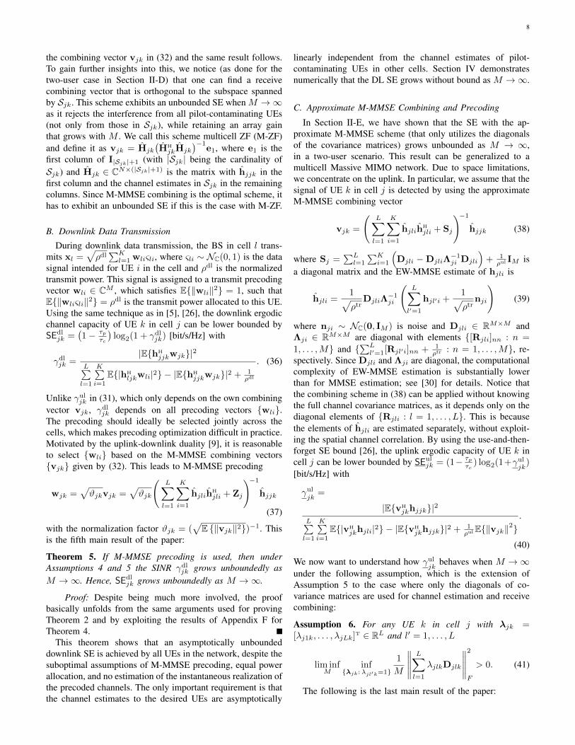
where fm ∼ N (0, σ2) and σ denotes the standard deviation.Fig. 2 shows the eigenvalue distribution with the three
covariance models above, for M = 100 antennas, uniformlydistributed AoAs θ in [−π,+π), β = 1, ∆ = 15◦, r = 0.5,and σ = 2. All three models create eigenvalue variations, butthere are substantial differences. The one-ring model providesrank-deficient covariance matrices, where a large fraction ofthe eigenvalues is zero (this fraction is computed in [11]).In contrast, the other two models provide full-rank covari-ance matrices with more modest eigenvalue variations. In theremainder, we consider the latter two models to emphasizethat our main results only require linear independence betweenthe covariance matrices, not rank-deficiency (which in specialcases give rise to orthogonal covariance supports [10]).
0 20 40 60 80 10010
−4
10−2
100
102
Eigenvalue (decreasing order)
Nor
mal
ized
val
ue
One−ring model (∆=15◦)Exponential correlation model (r=0.5)Uncorrelated, fading variations (2 dB)
Fig. 2: Average eigenvalue distribution with M = 100 and forthree different channel covariance models, whereof one gives a rank-deficient covariance matrix and the others have full rank.
BSUE 1UE 2
300 m
300
m Cell edge
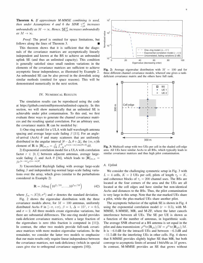
Fig. 3: Multicell setup with two UEs per cell in the shaded cell-edgearea. All UEs have similar AoAs to all BSs, which typically leads tosimilar covariance matrices and thus high pilot contamination.
A. Uplink
We consider the challenging symmetric setup in Fig. 3 withL = 4 cells, K = 2 UEs per cell, pilots of length τp = K,and coherence blocks of τc = 200 channel uses. The BSs arelocated at the four corners of the area and the UEs are alllocated at the cell edges and have similar but non-identicalAoAs and distances to the BSs. Thus, the pilot contaminationis very large in this setup. Note that the star-marked UEs sharea pilot, while the plus-marked UEs share another pilot.
The asymptotic behavior of the uplink SE is shown in Fig. 4using the exponential correlation model (r = 0.5), with M-MMSE, S-MMSE, MR, and M-ZF, where the latter cancelsinterference between all UEs. The SE per UE is shown asa function of the number of antennas, in logarithmic scale.The average SNR observed at a BS antenna is set equal in thepilot and data transmission: ρultr(Rjli)/M = ρtrtr(Rjli)/M .It is −6.0 dB for the intracell UEs and between −6.3 dB and−11.5 dB for the interfering UEs in other cells. Fig. 4 showsthat S-MMSE provides slightly higher SE than MR, but bothconverge to asymptotic limits of around 1 bit/s/Hz as M grows.In contrast, M-MMSE provides an SE that grows without

10
101
102
103
0
0.5
1
1.5
2
Number of antennas (M)
Spe
ctra
l effi
cien
cy [b
it/s/
Hz/
user
]
M−MMSES−MMSEMRCM−ZFTime splitting
Fig. 4: Uplink SE as a function of M , for covariance matrices basedon the exponential correlation model (r = 0.5).
bound. The instantaneous effective SINR grows linearly withM , which is in line with Theorem 4, as seen from the fact thatthe SE grows linearly when the horizontal scale is logarithmic.M-ZF performs poorly because the channel estimates areso similar that full interference suppression removes mostof the desired signal. In contrast, M-MMSE finds a non-trivial tradeoff between interference suppression and coherentcombining of the desired signal, leading to superior SE. Thereference curve “time splitting” considers the case when the 4cells are active in different coherence blocks, to remove pilotcontamination. MMSE combining is used and the SE growswithout bound, but at a slower pace than with M-MMSE, dueto the extra pre-log factor of 1/4. Hence, even for a smallsystem with L = 4, it is inefficient to avoid pilot contaminationby time splitting.
Next, we consider the uncorrelated Rayleigh fading modelin (42) with independent large-scale fading variations over thearray. The uplink SE with M = 200 antennas and varyingstandard deviation σ from 0 to 5 is shown in Fig. 5(a).M-MMSE provides no benefit over S-MMSE or MR in thespecial case of σ = 0, where the covariance matrices arelinearly dependent (i.e., scaled identity matrices). This is aspecial case that has received massive attention in academicliterature, mainly because it simplifies the mathematical anal-ysis. However, M-MMSE provides substantial performancegains over S-MMSE and MR as soon as we depart fromthe scaled-identity model by adding small variations in thelarge-scale fading over the array, which make the covariancematrices linearly independent. This is in line with what wedemonstrated in Example 2. As the variations increase, the SEwith M-ZF improves particularly fast and approaches the SEwith M-MMSE. M-ZF will never be the better scheme sinceM-MMSE is optimal. The motivation behind this simulationis the measurement results reported in [29], which show large-scale variations of around 4 dB over a massive MIMO array—this corresponds to σ ≈ 4 in our setup.
Fig. 5(b) shows the received power (normalized by the noisepower) after receive combining for an arbitrary UE when σ =4. It is divided into the desired signal power, the interferencefrom UEs using the same pilot, and the interference from UEsusing a different pilot. The figure shows that MR and S-MMSEsuffer from strong interference from the UEs that use the same
0 1 2 3 4 50
0.5
1
1.5
2
2.5
3
3.5
4
Standard deviation of fading variations over the array
Spe
ctra
l effi
cien
cy [b
it/s/
Hz/
user
]
M-MMSEM-ZFS-MMSEMR
(a) Uplink SE
Desired signal Interf: Same pilot Interf: Diff. pilot0
5
10
15
20
25
Rec
eive
d po
wer
ove
r no
ise
pow
er [d
B]
MRS−MMSEM−MMSEM−ZF
(b) Received signal power after receive combining
Fig. 5: Uplink with covariance matrices modeled by (42) for M =200 and K = 2. (a) The SE as a function of the standard deviationσ of the large-scale fading variations. (b) The received power afterreceive combining with σ = 4 is separated into desired signal powerand interference from UEs with the same or different pilot than thedesired UE.
pilot, since these schemes are unable to mitigate the coherentinterference caused by pilot contamination. In contrast, M-MMSE and M-ZF mitigate all types of interference and receiveroughly the same amount of interference from UEs with thesame or different pilots. Note that the price to pay for theinterference rejection is a reduction in desired signal powerwhen using M-MMSE and M-ZF.
B. Downlink
The setup in Fig. 3 is also used in the downlink whereinwe set ρdl = ρul to get the same SNRs as in the up-link. We consider a setup with both spatial channel corre-lation and large-scale fading variations over the array, suchthat the EW-MMSE estimator is suboptimal but Assump-tion 6 is satisfied. More precisely, we consider a combinationof the exponential correlation model and (42): [R]m,n =βr|n−m|eı(n−m)θ10(fm+fn)/20, where θ is the AoA, r = 0.5is used as correlation factor, and f1, . . . , fM ∼ N (0, σ2) giveindependent large-scale fading variations over the array withσ = 4.
The downlink SE is shown in Fig. 6 as a function ofM , where Fig. 6(a) shows results with the MMSE estimatorthat uses the full channel covariance matrices and Fig. 6(b)shows results with the EW-MMSE estimator that only usesthe diagonals of the covariance matrices. When using the
11
101
102
103
0
1
2
3
4
5
Number of antennas (M)
Spe
ctra
l effi
cien
cy [b
it/s/
Hz/
user
]
M−MMSEM−ZFS−MMSEMRT
(a) MMSE estimation
101
102
103
0
1
2
3
4
5
Number of antennas (M)
Spe
ctra
l effi
cien
cy [b
it/s/
Hz/
user
]
Approximate M−MMSEM−ZFApproximate S−MMSEMRT
(b) EW-MMSE estimation
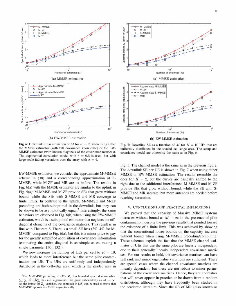
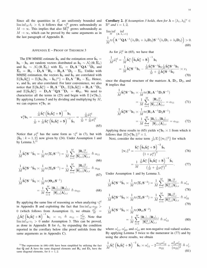
Fig. 6: Downlink SE as a function of M for K = 2, when using eitherthe MMSE estimator (with full covariance knowledge) or the EW-MMSE estimator (with known diagonals of the covariance matrices).The exponential correlation model with r = 0.5 is used, but withlarge-scale fading variations over the array with σ = 4.
EW-MMSE estimator, we consider the approximate M-MMSEscheme in (38) and a corresponding approximation of S-MMSE, while M-ZF and MR are as before. The results inFig. 6(a) with the MMSE estimator are similar to the uplink inFig. 5(a): M-MMSE and M-ZF provide SEs that grow withoutbound, while the SEs with S-MMSE and MR converge tofinite limits. In contrast to the uplink, M-MMSE and M-ZFprecoding are both suboptimal in the downlink, but they canbe shown to be asymptotically equal.7 Interestingly, the samebehaviors are observed in Fig. 6(b) when using the EW-MMSEestimator, which is a suboptimal estimator that neglects the off-diagonal elements of the covariance matrices. This result is inline with Theorem 6. There is a small SE loss (2%–4% for M-MMSE) compared to Fig. 6(a), but this is a minor price to payfor the greatly simplified acquisition of covariance information(estimating the entire diagonal is as simple as estimating asingle parameter [30], [32]).
We now increase the number of UEs per cell to K = 10,which leads to more interference but the same pilot contam-ination per UE. The UEs are uniformly and independentlydistributed in the cell-edge area, which is the shaded area in
7For M-MMSE precoding in (37), Zj has bounded spectral norm while∑l
∑i hjlih
Hjli has LK eigenvalues that grow unboundedly as M → ∞.
As the impact of Zj vanishes, the approach in [28] can be used to prove thatM-MMSE approaches M-ZF asymptotically.
101
102
103
0
1
2
3
4
5
Number of antennas (M)
Spe
ctra
l effi
cien
cy [b
it/s/
Hz/
user
]
M−MMSEM−ZFS−MMSEMRT
(a) MMSE estimation
101
102
103
0
1
2
3
4
5
Number of antennas (M)
Spe
ctra
l effi
cien
cy [b
it/s/
Hz/
user
]
Approximate M−MMSEM−ZFApproximate S−MMSEMRT
(b) EW-MMSE estimation
Fig. 7: Downlink SE as a function of M for K = 10 UEs that areuniformly distributed in the shaded cell edge area. The setup andcovariance model are otherwise the same as in Fig. 6.
Fig. 3. The channel model is the same as in the previous figure.The downlink SE per UE is shown in Fig. 7 when using eitherMMSE or EW-MMSE estimation. The results resemble theones for K = 2, but the curves are basically shifted to theright due to the additional interference. M-MMSE and M-ZFprovide SEs that grow without bound, while the SE with S-MMSE and MR saturate, but more antennas are needed beforereaching saturation.
V. CONCLUSIONS AND PRACTICAL IMPLICATIONS
We proved that the capacity of Massive MIMO systemsincreases without bound as M → ∞ in the presence of pilotcontamination, despite the previous results that pointed towardthe existence of a finite limit. This was achieved by showingthat the conventional lower bounds on the capacity increasewithout bound when using M-MMSE precoding/combining.These schemes exploit the fact that the MMSE channel esti-mates of UEs that use the same pilot are linearly independent,due to their generally linearly independent covariance matri-ces. For our results to hold, the covariance matrices can havefull rank and minor eigenvalue variations are sufficient. Thereare special cases where the channel covariance matrices arelinearly dependent, but these are not robust to minor pertur-bations of the covariance matrices. Hence, they are anomaliesthat will never appear in practice or be drawn from a randomdistribution, although they have frequently been studied inthe academic literature. Since the SE of MR (also known as

12
conjugate beamforming or matched filtering) generally has afinite limit, we conclude that this scheme is not asymptoticallyoptimal in Massive MIMO. Note that our results do not implythat the pilot contamination effect disappears; there is still aperformance loss caused by estimation errors and interferencerejection, but there is no fundamental capacity limit.
Most of our results assume that the full covariance ma-trices of the channels are known, but this is not a criticalrequirement. Theorems 3 and 6 proved that it is sufficientthat the diagonals of the covariance matrices are known andlinearly independent between pilot-sharing UEs; a conditionthat has been shown to hold for practical channels by themeasurements in [29]. Such statistical information can beaccurately estimated from only some tens of channel obser-vations [32], whereof some contain the desired signal plusinterference/noise and some contain only interference/noise.
The purpose of analyzing the asymptotic capacity whenM → ∞ is not that we advocate the deployment of BSswith a nearly infinite number of antennas—that is physicallyimpossible in a finite-sized world and the conventional channelmodels will eventually break down since more power isreceived than was transmitted. The importance of asymptoticsis instead what it tells us about practical networks with finitenumbers of antennas. For example, consider a network withany finite number of UEs that each have a finite-valued datarate requirement. Our main results imply that we can alwayssatisfy these requirements by deploying sufficiently manyantennas, even in the presence of pilot contamination. In fact,it is enough to have two channel uses per coherence block(one for pilot, one for data) to deliver any capacity value toany finite number of UEs. The linear M-MMSE scheme issufficient to achieve this in practice and interference can betreated as noise in the receivers, because the capacity lowerbounds that we considered rely on such simplifications.
APPENDIX A – USEFUL RESULTS
Lemma 3 (Theorem 3.4, Corollary 3.4 [35]). Let A ∈ CM×Mand x,y ∼ NC(0, 1
M IM ). Assume that A has uniformlybounded spectral norm and that x and y are mutually in-dependent and independent of A. Then, xHAx � 1
M tr(A),xHAy � 0 and E{|xHAx− 1
M tr(A)|p} = O(M−p/2).
Lemma 4 ( [36]). For any positive semi-definite M × Mmatrices A and B, it holds that 1
M tr (AB) ≤ ‖AB‖2 ≤‖A‖2‖B‖2, tr (AB) ≤ ‖A‖2tr (B) and tr
((I + A)−1B
)≥
11+‖A‖2 tr(B).
Lemma 5 (Matrix inversion lemma). Let A ∈ CM×M bea Hermitian invertible matrix, then for any vector x ∈ CMand any scalar ρ ∈ C such that A + ρxxH is invertiblexH(A + ρxxH)−1 = xHA−1
1+ρxHA−1x and (A + ρxxH)−1 =
A−1 − ρA−1xxHA−1
1+ρxHA−1x .Let U,C,V be matrices of compatible sizes,
then if C is invertible (A + UCV)−1
= A−1 −A−1U
(C−1 + VA−1U
)−1VA−1.
APPENDIX B – PROOF OF THEOREM 1
By applying Lemma 5, we may rewrite γul1 in (7) as
γul1 = M
(1
MhH
1 Z−1h1 −
∣∣∣ 1M hH
1 Z−1h2
∣∣∣21M + 1
M hH2 Z−1h2
)(43)
by also multiplying and dividing each term by M . UnderAssumption 1 and using Lemma 3 we have, as M →∞, that8
1
MhH
1 Z−1h1 �1
Mtr(Φ1Z
−1) , β11 (44)
1
MhH
2 Z−1h2 �1
Mtr(Φ2Z
−1) , β22 (45)
1
MhH
1 Z−1h2 �1
Mtr(Υ12Z
−1) , β12. (46)
Note that β11, β22, and β12 are non-negative real-valuedscalars, since the trace of a product of positive semi-definitematrices is always non-negative. Using this notation, it followsfrom Assumption 1 that9 lim infM β22 > 0 and we obtain
γul1
M� δ1 , β11 −
β212
β22. (47)
To proceed, notice that Assumption 2 implies the followingresult, as proved in Appendix C.
Corollary 1. If Assumption 2 holds, then for λ = [λ1, λ2]T ∈R2 and i = 1, 2,
lim infM
inf{λ:λi=1}
1
Mtr(Q−1
(λ1R1 + λ2R2
)Z−1
(λ1R1 + λ2R2
))> 0.
(48)
By expanding the condition in Corollary 1 for i = 1, wehave that
lim infM
infλ2
(β11 + λ2
2β22 + 2λ2β12
)> 0. (49)
By the definition of the lim infM operator, lim infM β22 >0 holds if and only if every convergent subsequence has anon-zero limit, i.e., limM β22 > 0. This ensures that, for anarbitrary convergent subsequence,
infλ2
(β11 + λ2
2β22 + 2λ2β12
)= β11 −
β212
β22= δ1 (50)
where the infimum is attained by λ2 = β12/β22. Substituting(50) into (49), implies that lim infM δ1 > 0. Therefore, wehave that γul
1 grows a.s. unboundedly and, thus, the first partof the theorem follows.
Since γul1 grows a.s. unboundedly and the logarithm is a
strictly increasing function, it follows that log2(1 + γul1 ) also
grows a.s. without bound. Moreover, since the almost suredivergence of a sequence of non-negative random variablesimplies the divergence of its expected value, it follows that alsoSEul
1 = (1− τp/τc)E{
log2
(1 + γul
1
)}grows without bound.
8Under Assumption 1, Q−1RiZ−1Rk has uniformly bounded spectral
norm, which can be easily proved using Lemma 4.9This can be proved by similar arguments as in Appendix C, since
tr(A2) ≥ (tr(A))2/rank(A) if A is Hermitian and A 6= 0.

13
APPENDIX C – PROOF OF COROLLARY 1 IN APPENDIX BConsider i = 1 and notice that the argument on the left-hand
side of (48) is lower bounded as1M ‖R1 + λ2R2‖2F
( 1ρtr + ‖R1 + R2‖2)( 1
ρul + ‖∑2k=1(Rk −Φk)‖2)
(51)
by applying Lemma 4 twice. The denominator of (51) isbounded from above due to Assumption 1 and independentof λ2. This proves that Assumption 2 is sufficient for (48) tohold for i = 1. The result for i = 2 follows by interchangingthe indices in the proof.
APPENDIX D – PROOF OF THEOREM 2We begin by plugging (13) into (12) to obtain
γdl1 =
|E {hH1 v1} |2
ϑ2
ϑ1E {|hH
1 v2|2}+ V{hH1 v1}+ 1
ρdlϑ1
. (52)
We need to characterize all the terms in (52) and begin withE {hH
1 v1}. Notice that E {hH1 v1} = E
{hH
1 v1
}since v1 is
independent of the zero-mean error h1. Then, we can expresshH
1 v1 as
hH
1 v1 =hH
1
(h2h
H2 + Z
)−1
h1
1 + hH1
(h2hH
2 + Z)−1
h1
=γul
1
1 + γul1
(53)
by first applying Lemma 5 and then identifying γul1 in (7) in the
numerator and denominator. Theorem 1 proves that γul1
M � δ1and applying this result to (53) yields hH
1 v1 � 1. By thedominated convergence theorem and the continuous mappingtheorem [35], we then have that |E{hH
1 v1}|2 � 1.Consider now the noise term 1
ρdlϑ1= E{‖v1‖2}
ρdl where ϑ1 =
(E{‖v1‖2
})−1. By applying Lemma 5 twice, we may rewrite
‖v1‖2 as
‖v1‖2 =hH
1
(h2h
H2 + Z
)−2
h1(1 + γul
1
)2=
1
M
1M hH
1
(h2h
H2 + Z
)−2
h1(1M + 1
M γul1
)2 . (54)
Let Re(·) denote the real-valued part of a scalar. The numer-ator in (54) can be expressed as
1
MhH
1 Z−2h1 − 2Re( 1
M hH1 Z−1h2
1M hH
2 Z−2h1)1M + 1
M hH2 Z−1h2
+1M hH
2 Z−2h2| 1M hH
2 Z−1h1|2(1M + 1
M hH2 Z−1h2
)2 (55)
by applying again Lemma 5 twice. Under Assumption 1 andby applying Lemma 3,
1
MhH
1 Z−2h1 �1
Mtr(Φ1Z
−2) , β′11 (56)
1
MhH
2 Z−2h2 �1
Mtr(Φ2Z
−2) , β′22 (57)
1
MhH
1 Z−2h2 �1
Mtr(Υ12Z
−2) , β′12 (58)
where β′11, β′22, and β′12 are non-negative real-valued scalars,since the trace of a product of positive semi-definite matricesis always non-negative. Therefore, we obtain
1
MhH
1
(h2h
H
2 + Z)−2
h1 � β′11 − 2β12β
′12
β22+β2
12β′12
(β22)2, δ′1.
(59)
Plugging (59) into (54) and using γul1
M � δ1 yields M‖v1‖2 �δ′1δ21
such that
1
ρdlϑ1=
E{‖v1‖2
}ρdl
� 1
Mρdl
δ′1δ21
. (60)
Consider now the two terms V{hH1 v1} and ϑ2
ϑ1E{|hH
1 v2|2}
.Similar to [5, Eq. (47)], we can upper bound V{hH
1 v1} asV{hH
1 v1} ≤ 2E {|hH1 v1 − E {hH
1 v1}|}+E{∣∣hH
1 v1
∣∣2}. Noticethat (by using E {hH
1 v1} � 1 and the dominated convergencetheorem) E {|hH
1 v1 − E {hH1 v1}|} � 0 and
E{∣∣hH
1 v1
∣∣2} = E{vH
1 (R1 −Φ1)v1
}(a)
≤ ‖R1 −Φ1‖2E{‖v1‖2
} (b)� 0 (61)
where (a) and (b) follow from Lemma 4 and E{‖v1‖2
}� 0
(since, as shown above, ‖v1‖2 � 1M
δ′1δ21� 0), respectively.
Therefore, we have that V{hH1 v1} � 0. Finally, we consider
ϑ2
ϑ1E{|hH
1 v2|2}
. By using (45), (46), and lim infM β11 > 0 (asfollows from Assumption 1), we have that
hH
1 v2(a)=
hH1
(h1h
H1 + Z
)−1
h2
1 + hH2
(h1hH
1 + Z)−1
h2
(b)=
1M hH
1 Z−1h2 −1M hH
1 Z−1h11M h1Z
−1hH2
1M + 1
M hH1 Z−1h1
1M + 1
M γul2
(c)�β12 − β11β12
β11
δ2= 0 (62)
where (a) and (b) follow from Lemma 5 after identifying10
hH2
(h1h
H1 + Z
)−1h2 as γul
2 (by also dividing and multiplyingby M ), and (c) follows by using (44), (46) and the fact that
γul2
M� δ2 , β22 −
β221
β11(63)
with lim infM δ2 > 0 (which follows from the proof ofTheorem 1 by interchanging UE indices). By applying Lemma3, this implies E
{|hH
1 v2|2}� 0. Observe now that ϑ2
ϑ1� δ′1
δ21
δ22δ′2
where δ′2 is obtained from δ′1 by interchanging UE indices.Since all the quantities in δ′1 are uniformly bounded (due toAssumption 1), lim infM δ1 > 0 (as proved in Appendix B)and lim infM δ2 < ∞ (since from (63) δ2 < β22 andlim infM β22 <∞ due to Assumption 1), we eventually havethat ϑ2
ϑ1E{|hH
1 v2|2}� 0.
Combining all the above results yields
γdl1
M� ρdl δ
21
δ′1. (64)
10The uplink SINR γul2 of UE 2 is obtained from (7) by interchanging UEindices.
14
Since all the quantities in δ′1 are uniformly bounded andlim infM δ1 > 0, it follows that γdl
1 grows unboundedly asM → ∞. This implies that also SEdl
1 grows unboundedly asM → ∞, which can be proved by the same arguments as inthe last paragraph of Appendix B.
APPENDIX E – PROOF OF THEOREM 3
The EW-MMSE estimate hk and the estimation error hk =hk − hk are random vectors distributed as hk ∼ NC(0,Σk)and hk ∼ NC(0, Σk) with Σk = DkΛ
−1QΛ−1Dk andΣk = Rk − DkΛ
−1Rk − RkΛ−1Dk − Σk. Unlike with
MMSE estimation, the vectors hk and hk are correlated withE{hkhH
k} = E{hk(hk − hk)H} = DkΛ−1Rk −Σk. Hence,
v1 and h1 are also correlated. For later convenience, we alsonotice that E{h1h
H1} = R1Λ
−1D1, E{h1hH2} = R1Λ
−1D2,and E{h2h
H1} = D2Λ
−1QΛ−1D1 = Θ21. We need tocharacterize all the terms in (25) and begin with E {vH
1 h1}.By applying Lemma 5 and by dividing and multiplying by M ,we can express vH
1 h1 as
vH
1 h1 =
1M hH
1
(h2h
H2 + S
)−1
h1
1M + 1
M hH1
(h2hH
2 + S)−1
h1
=1M µul
11M + 1
M µul1
.
(65)
Notice that µul1 has the same form as γul
1 in (7), but with{hk : k = 1, 2} now given by (24). Under Assumption 1 andby Lemma 3,11
1
MhH
1 S−1h1 �1
Mtr(Σ1S
−1) =1
M
M∑i=1
[R1]2i,i[S]i,i[Λ]i,i
, α11
(66)
1
MhH
2 S−1h2 �1
Mtr(Σ2S
−1) =1
M
M∑i=1
[R2]2i,i[S]i,i[Λ]i,i
, α22
(67)1
MhH
1 S−1h2 �1
Mtr(Θ21S
−1)
=1
M
M∑i=1
[R1]i,i[R2]i,i[S]i,i[Λ]i,i
, α12. (68)
By applying the same line of reasoning as when analyzing γul1
in Appendix B and exploiting the fact that lim infM α22 >
0 (which follows from Assumption 1), we obtain µul1
M =
1M hH
1
(h2h
H2 + S
)−1
h1 � υ1 , α11 − α212
α22. Note that
lim infM υ1 > 0 under Assumption 3. This can be proved,as done in Appendix B for δ1, by expanding the conditionreported in the corollary below (the proof unfolds from thesame arguments as in Appendix C).
11The expressions in (66)–(68) have been simplified by utilizing the factthat Q and Λ have the same diagonal elements and Rk and Dk have thesame diagonal elements, for k = 1, 2.
Corollary 2. If Assumption 3 holds, then for λ = [λ1, λ2]T ∈R2 and i = 1, 2,
lim infM
inf{λ:λi=1}
1
Mtr(Λ−1QΛ−1
(λ1D1 + λ2D2
)S−1
(λ1D1 + λ2D2
))> 0.
(69)
As for µul1 in (65), we have that
1
Mµul
1 =1
MhH
1
(h2h
H
2 + S)−1
h1
=1
MhH
1 S−1h1 −1M hH
1 S−1h21M hH
2 S−1h1
1M + 1
M hH2 S−1h2
� υ1
(70)
since the diagonal structure of the matrices Λ, D1, D2, andS implies that
1
MhH
1 S−1h1 �1
Mtr(R1Λ
−1D1S−1)
=1
M
M∑i=1
[R1]2i,i[S]i,i[Λ]i,i
= α11 (71)
1
MhH
2 S−1h1 �1
Mtr(R1Λ
−1D2S−1)
=1
M
M∑i=1
[R1]i,i[R2]i,i[S]i,i[Λ]i,i
= α12. (72)
Applying these results to (65) yields vH1 h1 � 1 from which it
follows that |E{vH1 h1}|2 � 1.
Next, consider the noise term 1ρul
E{||v1||2
}for which
‖v1‖2 =hH
1
(h2h
H2 + S
)−2
h1(1 + µul
1
)2 (76)
=1
M
1M hH
1
(h2h
H2 + S
)−2
h1(1M + 1
M µul1
)2 . (77)
Under Assumption 1 and by Lemma 3,
1
MhH
1 S−2h1 �1
Mtr(Σ1S
−2) =1
M
M∑i=1
[R1]2i,i[S]2i,i[Λ]i,i
, α′11
(78)
1
MhH
2 S−2h2 �1
Mtr(Σ2S
−2) =1
M
M∑i=1
[R2]2i,i[S]2i,i[Λ]i,i
, α′22
(79)1
MhH
1 S−2h2 �1
Mtr(Θ21S
−2)
=1
M
M∑i=1
[R1]i,i[R2]i,i[S]2i,i[Λ]i,i
, α′12 (80)
where α′11, α′22, and α′12 are non-negative real-valued scalars.By applying Lemma 5 twice to the numerator in (77) and byusing the above results, we obtain
1
MhH
1
(h2h
H
2 + S)−2
h1 � α′11 − 2α12α
′12
α22+α2
12α′22
(α22)2, υ′1.
(81)
15
(Aj,\k + Hjk,\jH
H
jk,\j
)−1
= A−1j,\k −A−1
j,\kHjk,\j(IL−1 + HH
jk,\jA−1j,\kHjk,\j
)−1
HH
jk,\jA−1j,\k. (73)
γuljk
M=
1
MhH
jjkA−1j,\khjjk −
1
MhH
jjkA−1j,\kHjk,\j
(1
MIL−1 +
1
MHH
jk,\jA−1j,\kHjk,\j
)−11
MHH
jk,\jA−1j,\khjjk. (74)
1
MA−1j,\k =
1
M
(∑l
∑i 6=k
hjlihH
jli + Zj
)−1
=1
M
(Hj,\kH
H
j,\k + Zj
)−1
=1
MZ−1j −
1
MZ−1j Hj,\k
(1
MIL(K−1) +
1
MHH
j,\kZ−1j Hj,\k
)−11
MHH
j,\kZ−1j (75)
Plugging (81) into (77) yields M‖v1‖2 � υ′1υ21
such that1ρul
E{||v1||2
}� 1
Mρul
υ′1υ21.
As for V{vH1 h1}, it can be easily proved (using the above
results and Lemma 3), that V{vH1 h1} � 0. Consider now the
interference term E{|vH
1 h2|2}
. Using (67) and (68), we have(by applying Lemma 5 and dividing and multiplying by M )that
vH
1 h2 =
1M hH
1
(h2h
H2 + S
)−1
h2
1M + 1
M µul1
=
1M hH
1 S−1h2 −1M hH
1 S−1h21M hH
2 S−1h2
1M + 1
M hH2 S−1h2
1M + 1
M µul1
�α12 − α12α22
α22
υ1= 0 (82)
where we have used the fact that 1M hH
1 S−1h2 � α12 and1M hH
2 S−1h2 � α22. Applying Lemma 3 to (82), we obtainE{|vH
1 h2|2}� 0.
Combining all the above results together yieldsγul
1
M �ρul υ
21
υ′1. Since all the components of υ′1 in (81) are uniformly
bounded and lim infM υ1 > 0 (under Assumption 3), itfollows that γul
1grows unboundedly as M →∞. Hence, SEul
1
also grows without bound.
APPENDIX F – PROOF OF THEOREM 4
We start by rewriting γuljk in (34) as
γuljk = hH
jjk
(∑l
∑i 6=k
hjlihH
jli + Zj︸ ︷︷ ︸Aj,\k
+∑l 6=j
hjlkhH
jlk︸ ︷︷ ︸Hjk,\jH
Hjk,\j
)−1
hjjk
(83)
where Aj,\k =∑l
∑i 6=k hjlih
H
jli + Zj is indepen-dent of {hjlk : l = 1, . . . L} and Hjk,\j =
[hj1k . . . hjj−1k hjj+1k . . . hjLk] ∈ CM×(L−1) collects allvectors hjlk with l 6= j (i.e., the channels of UEs that causepilot contamination). By Lemma 5, we obtain (73) at the top ofthe page. Plugging (73) into (83) and dividing both sides by Mleads to (74). By applying Lemma 5 once again, (75) followswhere Hj,\k ∈ CM×L(K−1) denotes the matrix collecting all
vectors hjli with i 6= k, which is independent of hjlk for anyj and l. Therefore, it follows that the first term in (74) is suchthat
1
MhH
jjkA−1j,\khjjk
(a)� 1
MhH
jjkZ−1j hjjk
(b)� 1
Mtr(ΦjjkZ
−1j ) , βjk,jj (84)
where (a) follows from Lemma 3 since hjjk and Hj,\k areindependent and thus 1
M hH
jjkZ−1Hj,\k � 0L(K−1) (remem-
ber that Hj,\k collects the L(K − 1) vectors {hjli} withi 6= k), and (b) follows from Lemma 3 by recalling thathjjk ∼ NC (0,Φjjk) where the matrices Φjjk can be proved(using Lemma 4) to have uniformly bounded spectral norm dueto Assumption 4. Using similar arguments, we have that thelth element of the row vector 1
M hH
jjkA−1j,\kHjk,\j ∈ C1×(L−1)
is such that[1
MhH
jjkA−1j,\kHjk,\j
]l
� 1
MhH
jjkZ−1j hjlk
� 1
Mtr(RjlkQ
−1jk RjjkZ
−1j ) , βjk,lj (85)
for l = 1, 2, . . . , L− 1. Furthermore, the (n,m)th element of1M HH
jk,\jA−1j,\kHjk,\j is
1
M
[HH
jk,\jA−1j,\kHjk,\j
]n,m� 1
MhH
jnkZ−1j hjmk
� 1
Mtr(RjmkQ
−1jk RjnkZ
−1j ) , βjk,mn. (86)
For notational convenience, let us define bjk ∈ RL−1 andCjk ∈ R(L−1)×(L−1) with entries[
bjk]l
= βjk,lj = vec
(1√M
Z−1/2j RjlkQ
−1/2jk
)H
vec
(1√M
Z−1/2j RjjkQ
−1/2jk
)(87)
and [Cjk
]l,n
= βjk,ln = vec
(1√M
Z−1/2j RjlkQ
−1/2jk
)H
vec
(1√M
Z−1/2j RjnkQ
−1/2jk
)(88)
where we have used the fact that tr(AB) = vec(AH)Hvec(B).In Appendix G, it is shown that, under Assumption 5, thefollowing corollary holds.
16
Corollary 3. If Assumption 5 holds, then for any UE k in cellj with λjk = [λj1k, . . . , λjLk]T ∈ RL and l′ = 1, . . . , L
lim infM
inf{λjk:λjl′k=1}
1
Mtr
(Q−1jk
( L∑l=1
λjlkRjlk
)Z−1j
( L∑l=1
λjlkRjlk
))> 0
(89)
and the matrix Cjk is invertible as M →∞.
Since Cjk is invertible as M → ∞ under Assumption 5,
we have thatγuljk
M in (74) is such that
γuljk
M� δjk , βjj,jk − bH
jkC−1jk bjk. (90)
Expanding condition (89) in Corollary 3 for l′ = j and usingthe definitions of bjk and Cjk yield
lim infM
infλjk
(βjj,jk + 2λ
T
jkbjk + λT
jkCjkλjk
)> 0 (91)
with λjk = [λj1k, . . . , λj(j−1)k, λj(j+1)k, . . . , λjLk]T ∈RL−1. The invertibility of Cjk as M → ∞ ensures that theinfimum exists for sufficiently large M and that it is given by
infλjk
(βjj,jk + 2λ
T
jkbjk + λT
jkCjkλjk)
= βjj,jk − bT
jkC−1jk bjk = δjk (92)
where the infimum is attained by λjk = C−1jk bjk. Substituting
(92) into (91) implies that lim infM δjk > 0. Therefore, γuljk
grows a.s. unboundedly and this implies that SEuljk grows
unboundedly as M → ∞, which can be proved as done inthe last paragraph of Appendix B.
APPENDIX G – PROOF OF COROLLARY 3 IN APPENDIX FThe argument of the left-hand side of (89) can be lower
bounded by1M
∥∥∑Ll=1 λjlkRjlk
∥∥2
F(1ρtr +
∥∥∑Ll=1 Rjlk
∥∥2
)(1ρul +
∥∥∑Ll=1
(Rjlk −Φjlk
)∥∥2
)(93)
by applying Lemma 4 twice. Notice that the denominator isbounded due to Assumption 5 and independent of {λljk}.Therefore, if (35) holds, it follows from (93) that (89) alsoholds.
We now exploit (89) to prove that Cjk is invertible forsufficiently large M . To this end, observe that Cjk with entriesgiven by (88) is a Gramian matrix obtained as the innerproducts of the vectors {ujlk = vec
(1√M
Z−1/2j RjlkQ
−1/2jk
):
∀l 6= j}. Therefore, as M grows large the matrix Cjk isinvertible if and only if the vectors {ujlk : ∀l 6= j} areasymptotically linearly independent. Notice that the condition(89) in Corollary 3 for l′ = j can be rewritten in compactform as
lim infM
inf{λjk:λjjk=1}
(ujjk +
∑l 6=j
λjlkujlk
)H(ujjk +
∑l 6=j
λjlkujlk
)> 0 (94)
which implies that the vectors {ujlk : ∀l} are asymptoti-cally linearly independent. Since any subset of a finite setwith linearly independent vectors is also linearly independent,(94) ensures that {ujlk : ∀l 6= j} are also asymptoticallylinearly independent. This proves that, under Assumption 5,the Gramian matrix Cjk is invertible as M → ∞ and thiscompletes the proof.
REFERENCES
[1] T. L. Marzetta, “Noncooperative cellular wireless with unlimited num-bers of base station antennas,” IEEE Trans. Wireless Commun., vol. 9,no. 11, pp. 3590–3600, Nov. 2010.
[2] E. G. Larsson, F. Tufvesson, O. Edfors, and T. L. Marzetta, “MassiveMIMO for next generation wireless systems,” IEEE Commun. Magazine,vol. 52, no. 2, pp. 186–195, Feb. 2014.
[3] J. G. Andrews, S. Buzzi, W. Choi, S. V. Hanly, A. Lozano, A. C. K.Soong, and J. C. Zhang, “What will 5G be?” IEEE J. Sel. AreasCommun., vol. 32, no. 6, pp. 1065–1082, Jun. 2014.
[4] E. G. Larsson and L. V. der Perre, “Massive MIMO for 5G,” IEEE 5GTech Focus, vol. 1, no. 1, 2017.
[5] J. Hoydis, S. Ten Brink, and M. Debbah, “Massive MIMO in the UL/DLof cellular networks: How many antennas do we need?” IEEE J. Sel.Areas Commun., vol. 31, no. 2, pp. 160–171, Feb. 2013.
[6] K. Guo, Y. Guo, G. Fodor, and G. Ascheid, “Uplink power controlwith MMSE receiver in multi-cell MU-massive-MIMO systems,” inProc. IEEE ICC, 2014, pp. 5184–5190.
[7] N. Krishnan, R. D. Yates, and N. B. Mandayam, “Uplink linear receiversfor multi-cell multiuser MIMO with pilot contamination: large systemanalysis,” IEEE Trans. Wireless Commun., vol. 13, no. 8, pp. 4360–4373,Aug. 2014.
[8] H. Ngo, M. Matthaiou, and E. G. Larsson, “Performance analysis oflarge scale MU-MIMO with optimal linear receivers,” in Proc. IEEESwe-CTW, 2012, pp. 59–64.
[9] X. Li, E. Bjornson, E. G. Larsson, S. Zhou, and J. Wang, “MassiveMIMO with multi-cell MMSE processing: Exploiting all pilots for in-terference suppression,” EURASIP Journal on Wireless Communicationsand Networking, no. 117, Jun. 2017.
[10] H. Yin, D. Gesbert, M. Filippou, and Y. Liu, “A coordinated approachto channel estimation in large-scale multiple-antenna systems,” IEEE J.Sel. Areas Commun., vol. 31, no. 2, pp. 264–273, Feb. 2013.
[11] A. Adhikary, J. Nam, J.-Y. Ahn, and G. Caire, “Joint spatial division andmultiplexing—the large-scale array regime,” IEEE Trans. Inf. Theory,vol. 59, no. 10, pp. 6441–6463, Oct. 2013.
[12] L. You, X. Gao, X.-G. Xia, N. Ma, and Y. Peng, “Pilot reuse for massiveMIMO transmission over spatially correlated rayleigh fading channels,”IEEE Trans. Wireless Commun., vol. 14, no. 6, pp. 3352–3366, Jun.2015.
[13] X. Gao, O. Edfors, F. Rusek, and F. Tufvesson, “Massive MIMOperformance evaluation based on measured propagation data,” IEEETrans. Wireless Commun., vol. 14, no. 7, pp. 3899–3911, Jul. 2015.
[14] M. Li, S. Jin, and X. Gao, “Spatial orthogonality-based pilot reuse formulti-cell massive MIMO transmission,” in Proc. WCSP, 2013.
[15] H. Q. Ngo and E. Larsson, “EVD-based channel estimations for multicellmultiuser MIMO with very large antenna arrays,” in Proc. IEEE ICASSP,2012.
[16] R. Muller, L. Cottatellucci, and M. Vehkapera, “Blind pilot decontami-nation,” IEEE J. Sel. Topics Signal Process., vol. 8, no. 5, pp. 773–786,Oct. 2014.
[17] D. Hu, L. He, and X. Wang, “Semi-blind pilot decontamination formassive MIMO systems,” IEEE Trans. Wireless Commun., vol. 15, no. 1,pp. 525–536, Jan. 2016.
[18] H. Yin, L. Cottatellucci, D. Gesbert, R. R. Muller, and G. He, “Robustpilot decontamination based on joint angle and power domain discrim-ination,” IEEE Trans. Signal Process., vol. 64, no. 11, pp. 2990–3003,Jun. 2016.
[19] J. Vinogradova, E. Bjornson, and E. G. Larsson, “On the separabilityof signal and interference-plus-noise subspaces in blind pilot decontam-ination,” in Proc. IEEE ICASSP, 2016.
[20] J. Zhang, B. Zhang, S. Chen, X. Mu, M. El-Hajjar, and L. Hanzo, “Pilotcontamination elimination for large-scale multiple-antenna aided OFDMsystems,” IEEE J. Sel. Topics Signal Process., vol. 8, no. 5, pp. 759–772,Oct. 2014.
17
[21] T. X. Vu, T. A. Vu, and T. Q. S. Quek, “Successive pilot contaminationelimination in multiantenna multicell networks,” IEEE Wireless Com-mun. Lett., vol. 3, no. 6, pp. 617–620, Dec. 2014.
[22] A. Ashikhmin and T. Marzetta, “Pilot contamination precoding in multi-cell large scale antenna systems,” in IEEE International Symposium onInformation Theory Proceedings (ISIT), 2012, pp. 1137–1141.
[23] L. Li, A. Ashikhmin, and T. Marzetta, “Pilot contamination precodingfor interference reduction in large scale antenna systems,” in Allerton,2013, pp. 226–232.
[24] E. Bjornson, J. Hoydis, and L. Sanguinetti, “Pilot contamination is nota fundamental asymptotic limitation in massive MIMO,” in Proc. IEEEICC, 2017.
[25] D. Neumann, M. Joham, and W. Utschick, “On MSE based receiverdesign for massive MIMO,” in Proc. SCC, 2017.
[26] T. L. Marzetta, E. G. Larsson, H. Yang, and H. Q. Ngo, Fundamentalsof Massive MIMO. Cambridge University Press, 2016.
[27] S. M. Kay, Fundamentals of Statistical Signal Processing: EstimationTheory. Upper Saddle River, NJ, USA: Prentice-Hall, Inc., 1993.
[28] E. Bjornson, M. Bengtsson, and B. Ottersten, “Optimal multiuser trans-mit beamforming: A difficult problem with a simple solution structure,”IEEE Signal Process. Mag., vol. 31, no. 4, pp. 142–148, Jul. 2014.
[29] X. Gao, O. Edfors, F. Tufvesson, and E. G. Larsson, “Massive MIMOin real propagation environments: Do all antennas contribute equally?”IEEE Trans. Commun., vol. 63, no. 11, pp. 3917–3928, Nov. 2015.
[30] N. Shariati, E. Bjornson, M. Bengtsson, and M. Debbah, “Low-complexity polynomial channel estimation in large-scale MIMO witharbitrary statistics,” IEEE J. Sel. Topics Signal Process., vol. 8, no. 5,pp. 815–830, Oct. 2014.
[31] C. Sun, X. Gao, S. Jin, M. Matthaiou, Z. Ding, and C. Xiao, “Beam divi-sion multiple access transmission for massive MIMO communications,”IEEE Trans. Commun., vol. 63, no. 6, pp. 2170–2184, Jun. 2015.
[32] E. Bjornson, L. Sanguinetti, and M. Debbah, “Massive MIMO withimperfect channel covariance information,” in Proc. ASILOMAR, 2016.
[33] S. Haghighatshoar and G. Caire, “Massive MIMO pilot decontaminationand channel interpolation via wideband sparse channel estimation,”CoRR, vol. abs/1702.07207, 2017.
[34] S. Loyka, “Channel capacity of MIMO architecture using the exponentialcorrelation matrix,” IEEE Commun. Lett., vol. 5, no. 9, pp. 369–371,Sep. 2001.
[35] R. Couillet and M. Debbah, Random matrix methods for wirelesscommunications. Cambridge University Press, 2011.
[36] A. W. Marshall, I. Olkin, and B. C. Arnold, Inequalities: theory ofmajorization and its applications, ser. Springer series in statistics. NewYork: Springer, 2011.
Emil Bjornson (S’07, M’12) received the M.S. de-gree in Engineering Mathematics from Lund Univer-sity, Sweden, in 2007. He received the Ph.D. degreein Telecommunications from KTH Royal Instituteof Technology, Sweden, in 2011. From 2012 to mid2014, he was a joint postdoc at the Alcatel-LucentChair on Flexible Radio, SUPELEC, France, and atKTH. He joined Linkping University, Sweden, in2014 and is currently Senior Lecturer and Docentat the Division of Communication Systems.
He performs research on multi-antenna commu-nications, Massive MIMO, radio resource allocation, energy-efficient com-munications, and network design. He is on the editorial board of the IEEETRANSACTIONS ON COMMUNICATIONS and the IEEE TRANSACTIONS ONGREEN COMMUNICATIONS AND NETWORKING. He is the first author ofthe textbooks Massive MIMO Networks: Spectral, Energy, and HardwareEfficiency (2017) and Optimal Resource Allocation in Coordinated Multi-CellSystems (2013). He is dedicated to reproducible research and has made a largeamount of simulation code publicly available.
Dr. Bjrnson has performed MIMO research for more than ten years andhas filed more than ten related patent applications. He received the 2016 BestPhD Award from EURASIP, the 2015 Ingvar Carlsson Award, and the 2014Outstanding Young Researcher Award from IEEE ComSoc EMEA. He hasco-authored papers that received best paper awards at WCSP 2017, IEEEICC 2015, IEEE WCNC 2014, IEEE SAM 2014, IEEE CAMSAP 2011, andWCSP 2009.
Jakob Hoydis (S’08–M’12) received the diplomadegree (Dipl.-Ing.) in electrical engineering and in-formation technology from RWTH Aachen Univer-sity, Germany, and the Ph.D. degree from Supelec,Gif-sur-Yvette, France, in 2008 and 2012, respec-tively. He is a member of technical staff at NokiaBell Labs, France, where he is investigating ap-plications of deep learning for the physical layer.Previous to this position he was co-founder andCTO of the social network SPRAED and worked forAlcatel-Lucent Bell Labs in Stuttgart, Germany. His
research interests are in the areas of machine learning, cloud computing, SDR,large random matrix theory, information theory, signal processing, and theirapplications to wireless communications. He is a co-author of the textbookMassive MIMO Networks: Spectral, Energy, and Hardware Efficiency (2017).He is recipient of the 2012 Publication Prize of the Supelec Foundation, the2013 VDE ITG Forderpreis, and the 2015 Leonard G. Abraham Prize of theIEEE COMSOC. He received the IEEE WCNC 2014 best paper award and hasbeen nominated as an Exemplary Reviewer 2012 for the IEEE Communicationletters.
Luca Sanguinetti (SM’15) received the LaureaTelecommunications Engineer degree (cum laude)and the Ph.D. degree in information engineeringfrom the University of Pisa, Italy, in 2002 and2005, respectively. Since 2005 he has been with theDipartimento di Ingegneria dell’Informazione of theUniversity of Pisa. In 2004, he was a visiting Ph.D.student at the German Aerospace Center (DLR),Oberpfaffenhofen, Germany. During the period June2007 - June 2008, he was a postdoctoral associate inthe Dept. Electrical Engineering at Princeton. During
the period June 2010 - Sept. 2010, he was selected for a research assistantshipat the Technische Universitat Munchen. From July 2013 to October 2017 hewas with Large Systems and Networks Group (LANEAS), CentraleSupelec,Gif-sur-Yvette, France.
Dr. Sanguinetti is currently serving as an Associate Editor for the IEEESIGNAL PROCESSING LETTERS. He served as an Associate Editor for IEEETRANSACTIONS ON WIRELESS COMMUNICATIONS, and as Lead Guest Edi-tor of IEEE JOURNAL ON SELECTED AREAS OF COMMUNICATIONS SpecialIssue on “Game Theory for Networks” and as an Associate Editor for IEEEJOURNAL ON SELECTED AREAS OF COMMUNICATIONS (series on GreenCommunications and Networking). Dr. Sanguinetti served as Exhibit Chairof the 2014 IEEE International Conference on Acoustics, Speech, and SignalProcessing (ICASSP) and as the general co-chair of the 2016 TyrrhenianWorkshop on 5G&Beyond. He is a co-author of the textbook Massive MIMONetworks: Spectral, Energy, and Hardware Efficiency (2017).
His expertise and general interests span the areas of communicationsand signal processing, game theory and random matrix theory for wirelesscommunications. He was the co-recipient of two best paper awards: IEEEWireless Commun. and Networking Conference (WCNC) 2013 and IEEEWireless Commun. and Networking Conference (WCNC) 2014. He was alsothe recipient of the FP7 Marie Curie IEF 2013 “Dense deployments for greencellular networks”.