Faculty of Science and Technology

MASTER’S THESIS

Study program/Specialization:

Petroleum Geosciences Engineering

Spring, 2015

Open

Writer:

David Thor Odinsson

(Writer’s signature)

Faculty supervisor: Nestor Cardozo

External supervisor(s): Lothar Schulte

Title of thesis:

Influence of seismic and velocity uncertainties on reservoir volumetrics

Credits (ECTS): 30

Keywords:

Uncertainty

Geostatistics

Volume attributes

Experimental design

Pages: 80

Stavanger, 15th

June, 2015

Copyright

by

David Thor Odinsson

2015

Influence of seismic and velocity uncertainties on reservoir

volumetrics

by

David Thor Odinsson, B.Sc.

Thesis

Presented to the Faculty of Science and Technology

The University of Stavanger

The University of Stavanger

June 2015

iv

Acknowledgements

This thesis report has been carried out at the department of petroleum

engineering at the University of Stavanger, Norway under the supervision of Nestor

Cardozo and Lothar Schulte.

I would like to acknowledge the University of Stavanger for providing the

workspace for the duration of this study.

I would like to thank Nestor Cardozo for reviewing my work and providing

me with helpful comments.

I express my sincere gratitude to Lothar Schulte for his dedication, countless

hours of inspirational discussions and providing helpful comments to accomplish this

study.

Finally, I would like to thank my family for their love and support during my

two years of study at the University of Stavanger.

v

Abstract

Influence of seismic and velocity uncertainties on reservoir

volumetrics

David Thor Odinsson, M.Sc.

The University of Stavanger, 2015

Supervisor: Nestor Cardozo; Lothar Schulte

Uncertainty is a well-known concept in geology, and can lead to re-evaluation

of important development decisions if properly assessed. This thesis describes

uncertainty through the set-up of “scenarios”. For each parameter used for the

structural model a so-called low case, base case and high case are defined. The

combination of the different cases results in many structural models that deliver a

distribution of the bulk volume. A generally acknowledged way of handling the large

number of models coming from the different combinations of the model parameters is

experimental design.

This study has shown that the uncertainty in the seismic picks and

consequently in the reservoir thickness have a large impact on the gross-volume. The

reservoir structural geometry controls the influence of fault uncertainty on the

reservoir volume. Well velocities used in this thesis for domain conversion are quite

accurate but sparsely sampled and therefore subject to uncertainty. In addition, the

vi

geologic complexity may have a dramatic influence on the uncertainty of the depth

conversion.

A proper assessment of seismic and velocity uncertainties can be applied to

risk analysis for field appraisal and development, hydrocarbon volume estimation,

accurate well placement, optimal well trajectory and reservoir history matching.

vii

Table of Contents

List of Tables ......................................................................................................... ix

List of Figures ..........................................................................................................x

1. Introduction .....................................................................................................1

2. Data .................................................................................................................8

3. Methodology .................................................................................................10

3.1 Well data .................................................................................................10

3.2 Capturing uncertainty in seismic interpretation ......................................14

3.2.1 Horizons ......................................................................................14

3.2.2 Faults ...........................................................................................18

3.2.3 Volume attributes ........................................................................19

3.3 Depth conversion based on well data......................................................21

3.4 Structural modeling .................................................................................24

3.5 Experimental Design ...............................................................................25

4. Observations ......................................................................................................30

4.1 Synthetic Seismogram observation .........................................................30

4.2 Seismic Interpretation and uncertainty estimation ..................................32

4.21. Horizons ......................................................................................32

4.2.2 Faults ...........................................................................................42

4.3 Depth conversion ....................................................................................45

4.3.1 Linear velocity law .....................................................................45

4.3.2 Blind well test for estimating uncertainty in depth .....................47

4.4 Uncertainty in gross-volume derived from modelled structural

uncertainty............................................................................................51

4.4.1 Numerical 3-D reservoir model ..................................................58

5. Discussion ..........................................................................................................61

5.1 Uncertainty in stratigraphic horizons ......................................................61

5.2 Uncertainty in fault position ...................................................................62

5.3 Uncertainty in depth conversion .............................................................63

5.4 Experimental design................................................................................63

viii

6. Conclusion .........................................................................................................65

References ..............................................................................................................66

ix

List of Tables

Table 1. Well information. .......................................................................................8

Table 2. Experimental design matrix. ....................................................................26

Table 3. Time error statistics. ................................................................................40

Table 4. Depth error statistics. ...............................................................................50

Table 5. Combinations and volume results of structural models for the Placket-

Burman experimental design. ..........................................................51

Table 6. Combinations and volume results of structural models for the full

factorial experimental design ............................................................53

Table 7. Explanation of the parameters and coefficients in the 25 term volume

equation. ............................................................................................56

Table 8. Random experimental run and its corresponding numerical 3-D model. 58

x

List of Figures

Figure 1. Stochastic simulation of geological surfaces using P-field simulation. ...4

Figure 2. Fault constructed from horizon fault lines. ...............................................5

Figure 3. Geological constraints on faults. ..............................................................7

Figure 4. Depth structure map outlining the area of interest. ..................................9

Figure 5. Sand and shale distribution in four wells. ..............................................10

Figure 6. Convolution model of a synthetic trace. .................................................12

Figure 7. Well-15, seismic well tie. .......................................................................13

Figure 8. High, base and low case of top reservoir. ...............................................15

Figure 9. High, base and low case reservoir time thickness for base case top

reservoir surface. ...............................................................................16

Figure 10. Reservoir time thickness uncertainty. ...................................................16

Figure 11. Experimental variogram. ......................................................................17

Figure 12. Fault uncertainty envelope. ..................................................................18

Figure 13. Fault slicing. .........................................................................................19

Figure 14. Original seismic vs. Structural smoothing............................................19

Figure 15. Original seismic vs. Cosine of instantaneous phase. ............................20

Figure 16. Ant track workflow...............................................................................21

Figure 17. Two linear velocity functions. ..............................................................22

Figure 18. Depth surface adjusted to wells. ...........................................................23

Figure 19. Time thickness map converted to depth. ..............................................24

Figure 20. Base reservoir depth surface constructed from depth thickness map. ..24

Figure 21. Structural modeling. .............................................................................25

Figure 22. Synthetic seismogram from Well-15. ...................................................30

Figure 23. Synthetic seismogram from well-15, well-14 and well-13. ................31

Figure 24. Time structure map of top reservoir. ....................................................32

xi

Figure 25. Section A. .............................................................................................33

Figure 26. Section A, frame 1. ...............................................................................34

Figure 27. Section A, frame 2. ...............................................................................34

Figure 28. Section B. .............................................................................................35

Figure 29. Section B, frame 1. ...............................................................................35

Figure 30. Section B, frame 2. ...............................................................................35

Figure 31. Section B, frame 3. ...............................................................................36

Figure 32. Section C. .............................................................................................36

Figure 33. Section C, frame 1. ...............................................................................37

Figure 34. Section C, frame 2. ...............................................................................37

Figure 35. Time error distribution due to statics....................................................38

Figure 36. Seismic intersections showing offset wells. .........................................39

Figure 37. Time error distribution of the top reservoir. .........................................40

Figure 38. Time error distribution of the reservoir thickness. ...............................40

Figure 39. Variogram analysis of time errors for top reservoir. ............................41

Figure 40. Variogram analysis of the reservoir thickness in the time domain. .....41

Figure 41. Section A. .............................................................................................42

Figure 42. Time slices from ant track volume. ......................................................43

Figure 43. Fault slicing of the northern fault. ........................................................44

Figure 44. Linear velocity law vs. checkshot interval velocities from Well-1 and

Well-15. ............................................................................................45

Figure 45. Problems in depth conversion.. ............................................................46

Figure 46. Difference map of the two depth surfaces using Convergent

Interpolation and Moving Average. ..................................................47

Figure 47. Depth structure map of top reservoir. ...................................................48

Figure 48. Depth error distribution of the top reservoir based on the blind well

test. ....................................................................................................48

xii

Figure 49. Variogram analysis of depth errors. .....................................................49

Figure 50. Thickness depth error distribution in the depth domain. ......................50

Figure 51. Variogram analysis of depth thickness errors. .....................................50

Figure 52. Placket-Burman experimental design. a) Observed volume vs.

Predicted volume. b) Residual plot. ..................................................52

Figure 53. Influence of parameters on the base case volume. ...............................53

Figure 54. Full factorial experimental design 25 terms. a) Observed volume vs.

Predicted volume. b) Residual plot. ..................................................55

Figure 55. Full factorial experimental design 25 terms. a) Observed volume vs.

Predicted volume. b) Residual plot ...................................................57

Figure 56. a) Volume distribution for 5000 calculations of the volume equation. b)

Cumulative density function of the volume distribution. .................58

Figure 57. Fault parameter values scaled to the interval [0,1]. ..............................59

Figure 58. Full factorial experimental design for 25 terms. a) Observed volume vs.

predicted volume, numerical model indicated with red circle. b)

Residual plot. ....................................................................................60

1

1. Introduction

Success in the oil and gas exploration and production (E&P) industry relies on

accurate positioning and interpretation of geological structures, as well as the use of

decision analysis. A proper assessment of seismic and velocity uncertainties can be

applied to risk analysis for field appraisal and development, accurate well placement,

optimal well trajectory, reservoir history matching and gross-rock volume estimation

(Vincent et.al., 1999; Thore et al., 2002 and Osypov et.al., 2011).

Experiments of uncertainties related to subsurface structures require a

geoscientist to create 3-D structural models. Structural models integrate different

types of data, e.g. 3-D/2-D seismic reflection surveys, borehole information, field

observations and analog models, each subject to different types of uncertainty. Data

most used for creating 3-D structural models of the subsurface are seismic images

obtained through seismic reflection surveys (Caers, 2011). Seismic reflection Surveys

follow the principles of seismology by generating artificial seismic waves and

measuring the time it takes the waves to travel from its source to a receiver on the

surface. Compiling and processing the travel time measurements results in an image

of the subsurface. Seismic images are a useful tool in creating three-dimensional

models but they are subject to inherent uncertainties, which directly affect the input

data for the structural model.

In a geologic context, uncertainty and error is easily confused. Uncertainty is

the recognition that our results may deviate from reality, whereas error expresses the

quantified uncertainty (Bárdossy et al., 2001). Mann (1993) studied uncertainty in

geology and classified uncertainties into three different types and listed possible

2

sources for each type. According to Mann (1993), Type I uncertainties refer to error,

bias and imprecision in the data. Type II uncertainties refer to stochasticity, for

example due to inhomogeneity and anisotropy in rock units. Type III uncertainties

refer to lack of knowledge or a need for generalization, predicting future or past

events for instance. Uncertainties of type I and II are quantitative and can be handled

by statistical methods, while uncertainties of type III are qualitative and theoretically

unknowable (Mann, 1993).

This thesis describes uncertainty through the set-up of “scenarios”. For each

parameter used for the structural model a so-called low case, base case and high case

are defined. The combination of the different cases results in many structural models

that deliver a distribution of the bulk volume. This distribution represents the bulk

volume uncertainty of the reservoir. A generally acknowledged way of handling the

large number of models coming from the different combinations of the model

parameters is experimental design. Experimental design is based on multiple linear

regression techniques to derive a volume equation capable of predicting the reservoir

volume for any combination of the model parameters.

The study area for this thesis is in the Gulf of Mexico. This region started to

form in the Middle to Late Triassic (230 Ma) as a result of intracontinental rifting

between the Yucatan and North America (Bird et al., 2005). According to Galloway

(2008), marine transgression into the continental area during the Middle Jurassic

resulted in the formation of extensive salt deposits. Tectonic activity during the Late

Cretaceous – Early Paleogene provided large quantities of terrigenous siliciclastic

sediments from uplifted source areas. This continued sediment influx resulted in the

accumulation of a wedge of Cenozoic deposits. These progradational deposits contain

3

reservoir, source, and seal units and are characterized by alternating sand reservoirs

and thick sealing shales. In addition, there are large growth faults and rollover

anticlines associated with tectonics, sedimentation and salt movement (Bascle et al.,

2001).

Many authors have contributed different techniques and methods for

estimating and quantifying uncertainty. For example, Thore et al., (2002) divided the

steps involved in the construction of a structural model into six phases: acquisition,

preprocessing, stacking, migration, interpretation and time-to-depth conversion and

discussed sources of uncertainty related to each phase. Their method to generate

multiple realizations of the structural model involves using a stochastic approach with

the algorithm of probability field simulation. This algorithm samples a local

conditional probability distribution that covers a range of possible outcomes of the

simulated variable, while forcing neighboring probability values to have some

similarities (Srivastava, 1992). First, a randomly selected value from the conditional

cumulative distribution function corresponding to a local probability value is added to

the base case surface (Figure 1). The local probability is correlated to the neighboring

nodes with a variogram describing the lateral correlation of the surface. In addition,

Thore et al., (2002) used a vertical variogram for intercorrelation between horizons.

Finally, the simulation is performed using any geostatistical methods that can

reproduce spatial correlation.

4

Figure 1. Stochastic simulation of geological surfaces using P-field simulation (Thore et al., 2002).

Samson et al., (1996) studied uncertainties related to stratigraphic horizons

through computing gross volume by stacking thickness maps of lithological units

below the top reservoir. In this way, they separated the uncertainty of the overburden

and the uncertainty of the reservoir units.

Faults are generally assumed as two-dimensional objects represented by

surfaces, “even though they are three-dimensional zones of deformation” (Røe et al.,

2014). This inevitably leads to uncertainty in their position and initial geometry when

digitizing them for instance, as “fault sticks” on seismic sections. Lecour et al., (2001)

applied a stochastic approach for fault modeling. Their method involves constructing

the faults by calculating the intersection of the horizons with the envelope of the fault

zone (horizons lines). These horizon limits are linearly interpolated within the fault

zone and the fault plane defined by the median line given by the mid points of the

5

interpolated lines (Figure 2). Their simulation methods involve the application of

probability field simulation controlled by a random function generator.

Figure 2. Fault constructed from horizon fault lines (Lecour et.al, 2001).

Velocity information is required for the time-to-depth conversion. Such

information can be derived from processing, i.e. seismic velocities or from well

measurements (Thore et al., 2002). Check-shot surveys and vertical seismic profiles

provide a highly accurate time-depth relationship. However, this velocity information

is limited to the borehole location and does not capture lateral variations (Hart, 2011).

Thore et al., (2002) applied cross validation technique by using the blind well test for

measuring the velocity uncertainties. However, the blind well test only delivers

reliable results for a large number of wells in the study area.

Following the division of Thore et al., (2002) for the steps involved in the

construction of a structural model, this thesis addresses uncertainties related to

interpretation and depth conversion. The analysis of the errors coming from

acquisition and processing are beyond the scope of this study.

6

Seismic uncertainties involve parameterizing and quantifying the uncertainty

of the reservoir location and the geometry of faults from interpreted seismic data in

the time domain. The structural uncertainty analysis of the reservoir model includes

the quantification of the uncertainty coming from the seismic interpretation in the

time domain. The reservoir under consideration consists of a top and a base horizon

captured by the seismic interpretation. Both horizons share a common source of

uncertainty coming from the overburden. This error includes static problems and

migration uncertainties of the seismic. The base reservoir horizon includes an

additional uncertainty coming from the reservoir thickness. The method outlined by

Samson et al., (1996), is applied so that the top reservoir horizon reflects the

uncertainty in the location of the reservoir, while the reservoir base is generated by

stacking thickness maps of lithological units below the top reservoir.

Fault geometries are constrained by basic geological rules explained in figure

3: they should not display inversion of curvature along the vertical axis and retain a

high wavelength of sinuosity along the horizontal axis for the reservoir interval

(Lecour et al., 2001). In addition, faults should retain their dip direction along the

horizontal axis.

7

Figure 3. Geological constraints on faults (Lecour, et.al, 2001).

Another major source for structural uncertainty is depth conversion. The blind

well test is an important tool to determine the velocity uncertainties and derive a depth

error distribution, representative for the whole area under investigation outside the

influence radius of the wells.

This thesis will differentiate itself from previous research in using

experimental design for describing the structural uncertainty analytically and

capturing the gross volume uncertainty of the reservoir through several thousand runs

of the volume equation with stochastically selected model parameter values. Finally, a

novel method is discussed that provides the possibility to set up a numerical 3-D

reservoir model for a parameter set used by any of the runs of the volume equation.

8

2. Data

The research area is covered by a 16.7 km2 of 3-D reflection seismic survey

consisting of 270 cross-lines and 220 in-lines with fifty-five feet spacing. The trace

length ranges from 0-3500 milliseconds (ms) with processing performed at four ms

sample interval. There are twenty-seven wells, of which twenty-five are inside the

research area with well log information. Table 1 shows the available well logs used in

this study for each well through the reservoir interval. Also available for these wells

are densely sampled check shot surveys that give accurate average velocity

measurements. The top and the base of the reservoir are defined by well tops and can

be identified by seismic events.

Table 1. Well information.

Well

name Reservoir interval

MD-Top (ft) MD-Base (ft) TWT-Top (ms) TWT-Base (ms) Gamma Density Neutron Sonic Well-1 6162.00 6241.00 1778.21 1797.22 X X X - Well-2 6130.00 6209.00 1779.70 1798.73 - - - X Well-3 6433.00 6548.00 1858.52 1885.78 - - - X Well-4 6468.00 6577.00 1802.97 1826.14 X - X X Well-5 5846.00 5912.00 1723.99 1740.16 - - - X Well-6 6427.00 6514.00 1818.04 1837.73 X - - X Well-7 6412.00 6528.00 1834.53 1860.78 - - - X Well-8 6536.00 6650.00 1860.31 1885.83 - - - X Well-9 - - - - X - - X Well-10 6536.00 6650.00 1834.26 1859.54 - - - X Well-11 6299.00 6435.00 1824.57 1856.97 - - - X Well-12 6413.00 6522.00 1839.92 1864.44 - - - X Well-13 6365.00 6502.00 1855.90 1888.48 X X - X Well-14 6663.00 6805.46 1910.04 1943.83 - X - X Well-15 6376.00 6498.00 1842.50 1871.34 X X X X Well-16 6227.00 6317.00 1796.14 1816.55 - - - X Well-17 6208.00 6298.00 1804.90 1826.23 - - - X Well-18 6593.00 6657.00 1629.82 1642.67 - - - X Well-19 5370.00 5405.00 1613.03 1621.96 - - - X Well-20 6237.00 6285.00 1751.76 1762.95 X - - X Well-21 6678.00 6804.00 1832.29 1859.81 - - - X

9

Well-22 6386.00 6493.00 1820.33 1844.76 - - - X Well-23 6474.00 6601.00 1868.65 1898.93 - - - X Well-24 6418.00 - 1792.80 - - - - X Well-25 6387.59 6444.54 1812.00 1824.94 - - - X Well-26 6179.00 6269.00 1797.15 1818.70 X - - X Well-27 Outside Outside Outside Outside Outside Outside Outside Outside Well-28 Outside Outside Outside Outside Outside Outside Outside Outside

The area of interest for the development of the methodology for this uncertainty

study consists of two horizons, top and base reservoir, and is bounded by two east-

west striking normal faults (Figure 4). The reservoir volume is calculated above the

oil water contact. The data in this study shows a salt dome in the western edge of the

seismic volume, outside the analyzed reservoir. The poor data quality near the salt

would have made an interpretation a challenge, given the time constraints.

Figure 4. Depth structure map outlining the area of interest.

OW

C

10

3. Methodology

This chapter discusses data calibration, uncertainty quantification, the steps

involved in creating structural models, and the method used to derive a distribution

for the gross volume of the reservoir.

3.1 WELL DATA

The reservoir under consideration shows characteristics of alternating shale

and sand bodies covered by a shale layer (Figure 5). The shale is characterized by

high GR (gamma-ray), RHOB (density) and NPHI (neutron porosity) values. The

sand shows low GR, RHOB and NPHI values. Using the cross-over display of RHOB

and NPHI, using a reverse scale for NPHI, allows to identify the sand bodies as

shown by Well-1 in figure 5. Based on the well log interpretation, the well tops were

defined for the top and base boundaries of the reservoir.

Figure 5. Sand and shale distribution in four wells. First track shows gamma ray log, second track shows neutron

and density logs.

11

The seismic is based on changes in the acoustic impedance, which typically

occur at lithological boundaries. The sonic log measures velocity on a frequency

range much higher than the seismic and typically starts several meters below datum

(Schlumberger, 2009). A checkshot survey provides more accurate seismic velocity

information at each checkshot point than the sonic log and allows for a better

comparison of the well data with the seismic. However, check shot surveys with large

check shot spacing can provide inaccurate time-depth information between the check

shot points. By calibrating the sonic log with a checkshot survey, a more accurate

time-depth relationship at the wells is derived. The principle of sonic calibration

involves fitting a drift curve to the check shot points (Schlumberger, 2009). First, the

drift curve is obtained by subtracting the integrated sonic times from the check shot

times. The resultant drift points are interpolated usually with a polynomial function.

Finally, the drift curve is added to the integrated sonic time, which is finally converted

to the calibrated sonic log. The final step establishes a link between the seismic and

the wells through generating a synthetic seismogram. The steps involved in

calculating the synthetic trace are shown in Figure 6. The sonic log (Dt) and density

log (ρ) are converted into the time domain with the help of the check shot survey. The

acoustic impedance log (AI) is derived from the sonic and the density log as:

AI = ρ ∗

1

𝐷𝑡 ( 3.1)

The reflectivity (RF) is derived from the acoustic impedance log:

𝑅𝐹𝑖 = (AIi+1 – AIi)

(AIi + AIi+1)

𝑖: 𝑛𝑢𝑚𝑏𝑒𝑟 𝑜𝑓 𝑠𝑎𝑚𝑝𝑙𝑒

(3.2)

12

Finally, the reflectivity is convolved with a wavelet, which results in the synthetic

trace.

Figure 6. Convolution model of a synthetic trace. First track shows density (blue) and sonic (black), second track

shows derived acoustic impedance, third track shows calculated reflectivity, fourth track shows Ricker wavelet,

fifth track shows synthetic seismog

The match between the synthetic trace and the seismic depends highly on the

wavelet. Often a so-called Ricker-wavelet with a user-defined mid-frequency is used.

Figure 7 shows the seismic well tie for Well-15. In the left-most track it shows the

sonic log (black) and the density log (blue). In the next track the reflectivity is shown.

It is convolved with the displayed Ricker wavelet, which delivers the synthetic trace

displayed in the middle of the seismic section, which is closest to the well location.

The last track (to the right) shows the correlation between the synthetic trace and the

13

seismic trace closest to the well position. The vertical axis is the “lag” axis. A

horizontal dashed white line marks the zero lag position. The match between the

synthetic and the seismic is done through adjusting the center frequency of the

wavelet. The maximum correlation, shown by a white asterix, should be at zero lag,

which means there is no shift between the synthetic and the seismic. In case of non-

zero lag, a constant shift needs to be applied to the synthetic in order to get a good

match with the seismic event. Finally, the time-depth relationship needs to be updated

to consider the final constant shift. The sign of the maximum correlation defines the

polarity of the seismic. A positive maximum correlation indicates SEG polarity; a

negative maximum correlation indicates European polarity.

Figure 7. Well-15, seismic well tie.

14

3.2 CAPTURING UNCERTAINTY IN SEISMIC INTERPRETATION

This study is based on the key assumption that well tops are correct even

though in reality there is uncertainty associated with well top determinations. A major

source of this uncertainty lies in the difficulty of correlating the events interpreted on

a well with the neighboring wells. Uncertainty coming from seismic interpretation is

captured by three interpretation versions reflecting the high case, base case and low

case. The high case results in a bulk volume increase and the low case in a bulk

volume decrease with respect to a reference case (base case).

3.2.1 HORIZONS

Making a reliable seismic well tie prior to the interpretation phase ensures that

the correct seismic event is being picked. Manual picking is required in areas of a low

signal-to-noise ratio where the seismic event is distorted (high uncertainty). Auto

tracking is automatically picking the seismic event through comparing the amplitudes

and cross correlation of neighboring traces within a small time-window (L. Schulte,

personal communication, March 25, 2015). It can be applied in areas of a coherent

seismic event. Auto tracking is a very efficient way of picking a horizon and delivers

a reproducible interpretation. 3-D guided auto tracking creates a dense interpretation

following the seismic event minimizing the need for manual interpretation. Applying

3-D seismic attributes that enhance the continuity of reflectors, such as structural

smoothing or cosine of instantaneous phase, assists in manually picking in areas of

high uncertainty (see section 3.2.3).

Typically, well tops do not accurately match the seismic event. They may

correspond to a different phase on the seismic image or show a small offset.

15

Measuring this time offset between the interpreted horizon and the well tops delivers

a two-way-time (TWT) error distribution. Only if the error distribution shows a non-

zero mean is the top reservoir surface shifted accordingly to acquire a Gaussian

distribution of the time errors. The standard deviation of this error distribution is used

to construct the high and low case horizons for the top reservoir. All horizons (low,

base and high case) are adjusted to the well tops (Figure 8).

Figure 8. High, base and low case of the top reservoir.

Constructing the low and high case for the reservoir base involves stacking

thickness maps below the top reservoir (Figure 9). The base case of the reservoir

thickness is derived from the tracked top and base horizons that are not adjusted to the

well tops. This thickness map is stacked below the top horizon that has been adjusted

to the well tops (Figure 10). Measuring the TWT error between the constructed

reservoir base and the well tops delivers the thickness uncertainty. The standard

16

deviation of the thickness error is used to construct the low and high case of the

thickness maps.

Figure 9. High, base and low case reservoir time thickness for base case top reservoir surface.

Figure 10. Reservoir time thickness uncertainty.

Variogram analysis of the time errors is used to determine the influence radius

of the wells used for the well top adjustment. The principles of deriving the variogram

Top reservoir

Top reservoir

Adjusted to wells

Base reservoir

Constructed

Base reservoir

17

function involves collecting point pairs separated by a so called “lag distance” to

describe the natural variation in the data in a specified direction (Caers, 2005). The

squared difference between all point pairs are gathered for a single value of variance

for a certain lag distance and repeated for different lag distances. An experimental

variogram plots these variance points against the corresponding lag distance, shown

as red circles in figure 11. A model variogram, represented by a spherical, Gaussian

or exponential function is fitted to the experimental variogram, shown by the black

curve in figure 11, where the data points of the experimental variogram appear to

flatten horizontally. Variance points that plot above the sill of the model variogram

are said to display no statistical similarities and the corresponding range is the spatial

correlation of the data in a specified direction (Caers, 2005). The variogram model is

needed by kriging or Gaussian simulation. For this study, the range of the variogram

model is used as input to the Petrel mapping algorithm that flexes the time and depth

surfaces to the well tops.

Figure 11. Experimental variogram.

Sem

ivari

an

ce

Separation distance

Sill

Range

Nugget

18

3.2.2 FAULTS

In seismic faults are characterized by amplitude variations, changes in

reflectors dip or reflector discontinuities/offsets. The 3-D seismic attributes that

measure these characteristics can be a powerful tool for fault detection. The ant track

workflow (see section 3.2.3) results in a volume that highlights the deformation zone

around the faults and provides the possibility of drawing polygons outlining the fault

envelope. The envelope represents the uncertainty in the fault interpretation that

approximates the 3D fault zone by a fault plane. All polygons drawn on several time

slices are gathered forming a couple of hanging wall – footwall sets for each fault

describing the high and low case. A median line is computed and linked to each set to

create the base case fault (Figure 12). This method ensures that the median line is

nearly centered on the ant tracked event.

Figure 12. Fault uncertainty envelope. Median line (green) calculated between high case (red) and low case (blue).

Fault slicing provides a way to quality check the assumed width of the fault

envelope by projecting the ant track volume onto the base case fault plane. The fault

19

plane is translated by a certain user-defined distance into the hanging wall and

footwall. This process is called fault slicing and allows observing amplitude changes

(Figure 13) at the edges of the fault zones that are characterized by the onset of the

high amplitudes.

Figure 13. Fault slicing. Ant track volume projected onto the base case fault surface (middle) showing amplitude

changes with a step-out distance of 100 feet into the hanging wall (left) and footwall (right).

3.2.3 VOLUME ATTRIBUTES

Structural smoothing performs data smoothing of the input signal by applying

Gaussian weighted average filtering following the trend of the seismic events after

determining the local dip and azimuth of the structure (Schlumberger, 2010). This

attribute increases the signal-to-noise ratio, which can be useful for structural

interpretation (Figure 14).

Figure 14. Original seismic (left) vs. Structural smoothing (right).

20

Cosine of instantaneous phase as the name suggests is the cosine function of

the instantaneous phase angle φ(t). Mathematically, the instantaneous phase is given

by:

𝜑(𝑡) = tan−1[(𝑔(𝑡) 𝑓(𝑡)⁄ )] (3.3)

f(t) is the real part of the complex seismic signal and g(t) its imaginary part

(Schlumberger, 2010). This attribute is linked to the instantaneous phase and therefore

not sensitive to amplitude variations (L. Schulte, personal communication, March 25,

2015). The peak of the cosine of instantaneous phase is at the position of the seismic

amplitude peaks, its troughs located at the seismic amplitude troughs. Therefore, it is

possible to track a seismic horizon on this attribute. Often in noisy or complex areas,

it is easier to interpret on the cosine of instantaneous phase than on the original

seismic cube because of its amplitude-independent character. Figure 15 shows the

same section of the original seismic and of the cosine of instantaneous phase cube.

Obviously, it is easier to follow the seismic events on the attribute cube because the

amplitude dependence is gone.

Figure 15. Original seismic (left) vs. Cosine of instantaneous phase (right).

Ant tracking uses the principles of swarm intelligence to extract events shown

by high amplitudes in a preconditioned seismic cube (Figure 16). Typically the

21

attribute processes chaos or variance are applied to the seismic cube. Both attributes

highlight the discontinuities in the seismic signal and hence are optimum for fault

detection. Ant tracking deploys agents (ants) on the preconditioned volume. Each ant

agent searches for local maxima and tries to follow these events (faults). The

parameter control allows the user to apply constraints to the ant agents, which defines

the number of tracked faults and the quality (coherent noise) of the ant track volume

(Schlumberger, 2010).

Figure 16. Ant track workflow. Original seismic (top left), Structural smoothing (bottom left), variance (top right)

and ant track (bottom right).

3.3 DEPTH CONVERSION BASED ON WELL DATA

The interpretation is done in the time domain, but the volume calculation must

be done in the depth domain. Therefore, time-to-depth conversion is necessary. Using

the linear velocity law in a layer cake model down to the top of the reservoir should

take into account major velocity boundaries of the overburden layers to get a more

accurate depth of the top reservoir. The velocity model process (Petrel) offers two

22

types of linear velocity functions (Figure 17). Both functions give the same result at

the wells, but derive the V0 at different locations. K is the slope of the linear velocity

law and describes the increase in velocity with depth. Therefore, K is related to

compaction. The K value of the velocity law for each layer is the average of the k

value derived at each well for the layer under consideration. It is kept constant since

compaction is considered as a regional event. As this project deals with a thin

reservoir interval velocities are used to depth convert the reservoir time thickness. The

calculation of the interval velocities is based on the well top depths and the surface

times at the well top positions.

Figure 17. Two linear velocity functions (Schlumberger, Petrel manual, Velocity modeling course, 2009) (edited

by author).

The depth error of the top reservoir coming from the velocity uncertainty is

estimated with a blind well test. The velocity model is set up based on all wells with

the exception of one well. The difference between the depth surface and the well top

depth of the left out well is measured. This process is repeated for all wells to get a

distribution of the depth errors. The assumption is that this error distribution describes

the depth uncertainty at any location of the depth surface outside the radius of

23

influence of the wells. In practical terms, this means that the depth error of the surface

at the position of a new well lies within the depth error distribution derived by the

blind well test. The depth error standard deviation is used to derive the low and high

case of the depth surface describing the top reservoir.

The estimation of the depth error of the reservoir base is done in two steps.

First, the depth surface of the reservoir top is adjusted to the well tops (Figure 18).

Second, the depth uncertainty of the reservoir base is estimated by applying a constant

interval velocity to the reservoir time layer (L. Schulte, personal communication,

March 25, 2015) (Figure 19). The constant velocity is estimated through averaging the

interval velocities derived at all wells. The depth thickness resulting from the constant

interval velocity is stacked below the reservoir top giving the reservoir base (Figure

20). The well tops at the reservoir base deliver the depth error distribution describing

the uncertainty of the reservoir base surface.

Figure 18. Depth surface adjusted to wells. Intersect given in figure 19.

24

Figure 19. Time thickness map converted to depth.

Figure 20. Base reservoir depth surface constructed from depth thickness map. Intersect given in figure 19.

3.4 STRUCTURAL MODELING

The goal of building the 3-D models for this study is to calculate reservoir

volumes. Figure 21 illustrates the three steps involved in creating a structural model in

the used modeling package (Petrel). The first step defines the fault planes of the

25

geological model as a set of linear key pillars that form the basis of creating the 3-D

grid. The second step uses the pillars from the faults to construct a skeleton grid,

which guides the geometry of the final 3-D grid. The final step is to insert horizons

and, if necessary, zones defined by well tops only into the skeleton grid. This process

defines the 3-D grid. Often modeling the seismic horizons require manual editing to

ensure that the horizon-fault intersects are correct.

Figure 21. Structural modeling. Fault modeling (left), pillar gridding (middle) and horizon modeling (right).

3.5 EXPERIMENTAL DESIGN

Experimental design applies multiple linear regression analysis to several

independent variables (X) to make an analytical relationship with a measurable output

(Vpred). The used method assumes a linear relationship between X and Vpred,

represented by a proxy equation:

𝑉𝑝𝑟𝑒𝑑 = 𝛽0 + 𝛽1𝑋1 + 𝛽2𝑋2 … 𝛽𝑛𝑋𝑛 (3.4)

where the βn coefficients reflect the contribution to the output of each

corresponding Xn factor, where n is the number of factors under consideration. The

factors represent the model parameters. This study considers six parameters, i.e. two

faults, time horizon, time thickness, depth horizon and depth thickness. Vpred is the

26

predicted reservoir volume based on the value of the parameters. In order to solve the

coefficients (βn) a set of linear equations (n+1) for different parameter sets and

corresponding reservoir volumes is solved through multiple linear regression analysis.

The parameters can have values within the range of [-1, 1] with minus one describing

the low case, zero the base case and plus one the high case parameter. Table 2 shows

the matrix of the screening design used and the parameter sets for which the reservoir

volume needs to be calculated. This involves building 3D models using these

parameter sets and calculating the requested volumes.

Table 2. Experimental design matrix.

Exp # Fault1 Fault2 HorizonT ThicknessT HorizonD ThicknessD Resp_Volume 1 1 -1 1 -1 -1 -1

2 -1 -1 -1 -1 -1 -1 3 -1 -1 1 1 1 -1 4 1 1 1 -1 1 1 5 1 1 -1 1 -1 -1 6 1 -1 -1 -1 1 1 7 0 0 0 0 0 0 8 -1 1 1 1 -1 1 9 -1 1 1 -1 1 -1 10 1 1 -1 1 1 -1 11 1 -1 1 1 -1 1 12 -1 1 -1 -1 -1 1 13 0 0 0 0 0 0 14 -1 -1 -1 1 1 1

For example, consider a linear equation describing the reservoir volume as a

function of one parameter (Horizon):

𝑉𝑝𝑟𝑒𝑑 = 𝛽0 + 𝛽1 ∗ 𝐻𝑜𝑟𝑖𝑧𝑜𝑛 (3.5)

27

First, the coefficients β0 and β1 are calculated from two equations with the

parameters and volumes given below:

Experiment Horizon Response Volume (V)

1 0 30

2 -1 10

The first equation is the centerpoint of the regression model, and delivers the

value of the β0 coefficient (30). Subsequently, the β1 coefficient is derived using

simple algebra,

𝛽1 =𝑉 − 𝛽0

𝐻𝑜𝑟𝑖𝑧𝑜𝑛= 20

With,

𝑉 = 10

𝐻𝑜𝑟𝑖𝑧𝑜𝑛 = −1

𝛽0 = 30

Now the reservoir volume distribution can be computed by solving the

equation (5) several hundred times through stochastically varying the parameter

values within the range [-1, 1] as shown below.

Prediction Horizon Predicted Volume (Vpred)

1 -0.2 26

2 0.91 48.2

3 1 50

28

4 0.34 36.8

This study applies a Plackett-Burman design (Plackett et al., 1946) for

screening the reservoir parameters in order to understand their influence on the

volume. Screening designs assume that all interactions are negligible this delivers a

less accurate proxy equation (3.6). The number of experimental runs required is

dependent on the parameters under consideration and the saturation level of the

model. The benefit of Placket-Burman designs, as implemented in the used software

(Essential Experimental Design, (Steppan et al., 1998)), is that they only require

twelve experimental runs plus two centerpoints for up to eleven factors. In other

words, they utilize all degrees of freedom to estimate the main terms (Steppan et al.,

1998). These results are accurate enough for identifying the most influential

parameters on the calculated volume.

𝑉𝑝𝑟𝑒𝑑 = 𝛽0+𝛽1𝑋1+𝛽2𝑋2+𝛽3𝑋3+𝛽4𝑋4+𝛽5𝑋5+𝛽6𝑋6 (3.6)

The uncertainty analysis of the reservoir volume is based on those coefficients that

contribute more than 5% to the total volume.

Based on the most influential parameters a two-level full factorial

experimental design has been selected for setting up the proxy equation used for

predicting the volume distribution resulting from the parameter uncertainties. A two-

level full factorial design includes two- and three-way interactions in addition to the

main terms. A two-level full factorial design requires 2n experimental runs and two

centerpoints, where the constant 2 represents the high and low setting coming from

29

each factor and n represents the number of factors used to model the predicted volume

(Steppan et al., 1998).

𝑉𝑝𝑟𝑒𝑑 = 𝛽0+𝛽1𝑋1+𝛽2𝑋2+𝛽3𝑋3+𝛽4𝑋4+𝛽5𝑋5+𝛽6𝑋6+𝛽7𝑋1𝑋2 + ⋯

+ 𝛽𝑎𝑋1𝑋2𝑋3 + ⋯

(3.7)

The number of terms in the full factorial proxy equation (3.7) is dependent on

the results from the screening design. Equation 3.7 can contain statistically

insignificant terms. Backward elimination measures the significance value for each

term, where low values indicate high model significance (Steppan et al., 1998). If a

term exceeds a preconditioned significance value it is not included in the volume

equation. The resulting equation, with fewer terms, is regarded as the best-fit model to

predict the volume.

30

4. Observations

4.1 SYNTHETIC SEISMOGRAM OBSERVATION

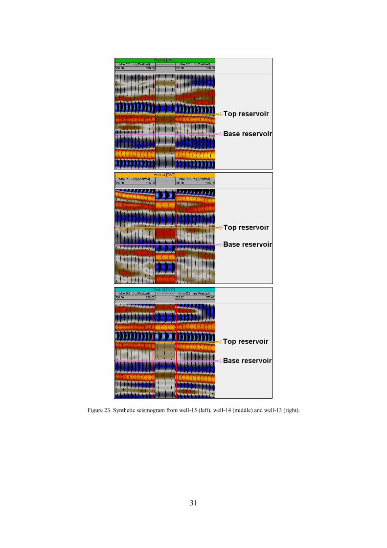
Synthetic seismograms were constructed for three wells that have sonic and

density logs covering the reservoir interval to identify the geologic events on the

seismic data. Figure 22 shows that the seismic data has SEG polarity: the upper part

of the figure shows the synthetic trace in inverse polarity, the lower part shows the

normal polarity. The correlation trace gives maximum positive correlation for the

synthetic trace in SEG polarity. A zero crossing between a strong peak reflection and

a trough features the top of the reservoir on the synthetic traces of all three wells

(Figure 23). The base of the reservoir is not as clearly defined and alternates between

a faint peak reflection and an s-crossing, i.e. where the amplitude is zero between a

trough at the top and peak reflector at the bottom.

Figure 22. Synthetic seismogram from Well-15. First track shows a Ricker wavelet, which delivers the synthetic

trace displayed in the middle of the seismic section. The last track (to the right) shows the correlation between the

synthetic trace and the seismic trace closest to the well position.

31

Figure 23. Synthetic seismogram from well-15 (left), well-14 (middle) and well-13 (right).

32

4.2 SEISMIC INTERPRETATION AND UNCERTAINTY ESTIMATION

4.21. Horizons

To illustrate the uncertainty in seismic interpretation requires the analysis of

seismic sections with focus on comparing the original seismic volume with attribute

cubes in areas of uncertainty, such as low signal-to-noise. Three random seismic lines

crossing key wells were created for this purpose (Figure 24).

Figure 24. Time structure map of top reservoir, shows selected wells and seismic intersections.

These areas of uncertainty can be identified based on the following classification:

Class 1: Weak semi-continuous amplitude

33

Class 2: Low signal-to-noise ratio resulting in discontinuities

The navigation of the seismic sections discussed in the following is given in

Figure 24. The frames shown in black on sections A – C (Figure 25, 28 and 32)

correspond to the enlarged sections to highlight the areas of uncertainty. The seismic

sections show that the top reservoir seismic event (shown in green) is tracked on a

zero crossing between peak and trough reflectors with strong amplitudes. The base

reservoir seismic event (shown in yellow) is tracked on a zero crossing between

trough and peak reflectors with weak semi-continuous amplitudes.

In frame 1 and 2 on section A (Figure 25), strong amplitudes characterize the

top reservoir throughout the section; whereas the base reservoir features class 1 and 2

uncertainties (Figure 26a and 27a). The cosine of instantaneous phase provides a

better continuity of the base reservoir seismic event for the interpretation, which

allows tracking the horizon in this area with more confidence (Figure 26b and 27b).

Figure 25. Section A, intersect shown on figure 24.

12

34

Figure 26. Section A, frame 1.

Figure 27. Section A, frame 2.

In frame 1 on section B (Figure 28), the two seismic events display class 1

uncertainty near a minor fault (Figure 29a). The structural smoothing attribute

enhances the continuity of the downthrown events significantly (Figure 29b). In frame

2, the top reservoir horizon features class 1 uncertainty, and the base class 1 and 2

uncertainties (Figure 30a). Again, structural smoothing enhances the continuity of the

top reservoir horizon, although on cost of the resolution, which is decreased near the

base horizon (Figure 30b). In frame 3, the top reservoir features class 1 uncertainty,

and the base class 1 and 2 uncertainties (Figure 31a). Structural smoothing enhances

continuity and increases the signal-to-noise ratio (Figure 31b).

a b

a b

35

Figure 28. Section B, intersect shown on figure 24.

Figure 29. Section B, frame 1.

Figure 30. Section B, frame 2.

1

2 3

a b

a b

36

Figure 31. Section B, frame 3.

In frame 1 on section C (Figure 32), the top and base horizons feature class 1

uncertainty (Figure 33a). Structural smoothing enhances seismic continuity for the top

horizon only (Figure 33b). In frame 2, the top reservoir horizon shows characteristics

of strong amplitudes, whereas the base reservoir horizon features class 1 uncertainty

(Figure 34a). Cosine of instantaneous phase provides better continuity of the base

reservoir seismic event (Figure 34b).

Figure 32. Section C, intersect shown on figure 24.

a b

1

2

37

Figure 33. Section C, frame 1.

Figure 34. Section C, frame 2.

A difference map of the original seismic volume and a smoothed volume

shows that uncertainties due to statics have a Gaussian distribution with a standard

deviation of ± 1.32 ms (Figure35).

a b

a b

38

Figure 35. Time error distribution due to statics.

Tops on three wells show significant offset with respect to the seismic event

(Figure 36). Well-11 and Well-8 are both in the vicinity of the tied Wells 13 and 14

respectively (Figure 36a and b). The tops of Well-19 are located on a different phase

positioned in an isolated fault segment (Figure 36c). Following the seismic event

linked to these well tops will result in a conflict with the interpretation supported by

the other wells. Therefore, wells 8, 13 and 19 are not included in the uncertainty

study.

39

Figure 36. Seismic intersections showing offset wells.

The time error between the interpreted top reservoir horizon and each well top

gives a distribution of time errors (Figure 37). Table 3 summarizes the time error

statistics, of the top reservoir horizon and the reservoir thickness, used for

constructing the high and low cases. The mean error of -1.83 ms for the top reservoir

indicates that the geological event is about 2 ms below the tracked zero crossing.

Applying the shift of -1.83 ms to the top reservoir results in a normal error

distribution with zero mean. The base reservoir is constructed through stacking the

reservoir time thickness below the top reservoir as discussed in the Methodology. The

time error for the reservoir base is resulting from the reservoir thickness uncertainty

(Figure 38).

a b

c

40

Figure 37. Time error distribution of the top reservoir.

Figure 38. Time error distribution of the reservoir thickness.

Table 3. Time error statistics.

Top reservoir (ms) Reservoir thickness (ms) Mean -1.83 0 std.dev. 7.38 6.55 Variance 54.46 42.94

The sample variograms shown in Figure 39 and 40 define the spatial

correlation of the time errors. The variogram model fitted to the variance points of the

time errors shows that the influence radius of the wells (variogram range) has a range

41

of 600 feet for the top reservoir and 1000 feet for the reservoir thickness (Figure 39

and 40). These measurements are used for adjusting the top and base reservoir cases

to the well tops.

Figure 39. Variogram analysis of time errors for top reservoir, shown in figure 37.

Figure 40. Variogram analysis of the reservoir thickness in the time domain, shown in figure 38.

42

4.2.2 Faults

The ant track volume captures the two faults outlining the reservoir fairly well

within most of the seismic volume (e.g. section A, Figure 41). The time lines of the

ant tracking time slices in Figure 42 are also included in Figure 41. In Figure 41 and

42 the faults representing the base case are shown in green, the faults capturing the

fault zone outline are shown in red and blue. Both faults are represented by the offset

of strong amplitudes in the reservoir. However, the southern fault shows more

bifurcation on the ant tracking time slices resulting in a wider uncertainty envelope. In

addition, the westernmost area between -1700 and -1900 ms shows the southern fault

changing its strike significantly. Here the characteristics for fault detection are weak

and not captured by the ant track volume (Figure 41 and 42). The continuation of the

fault can be seen below -1900 ms, where it is truncated by the northern fault.

Figure 41. Section A, intersect shown on figure 42 (top left).

A A’

-1400 ms

-1800 ms

-1500 ms

-1600 ms

-1700 ms

-1900 ms

43

Figure 42. Time slices from ant track volume.

-1400 ms -1500 ms

-1600 ms -1700 ms

-1800 ms -1900 ms

A

A’

44

The apparent average thicknesses of the northern and southern faults defined

by the fault envelopes are 466 ft and 765 ft, respectively. These thicknesses were

calculated from the difference between polygon nodes in a consecutive order (see

Figure 12). In order to quality check the apparent thickness of the fault envelope fault

slicing has been applied. Figure 43 shows the fault slicing results for the northern

fault using a step-out distance of 150 and 233 ft. Most of the amplitudes fade out at a

step out distance of ± 233 ft from the base case fault. The bifurcation and low quality

imaging of the southern fault yields imperceptible results.

Figure 43. Fault slicing of the northern fault.

Hanging wall 233 ftHanging wall 150 ft

Foot wall 150 ftFoot wall 233 ft

Nearest

45

4.3 DEPTH CONVERSION

4.3.1 Linear velocity law

Figure 44 shows the relationship between the interval velocities coming from

the check shots and the derived linear velocity law for two wells. The check shot

velocities show a velocity boundary marked as the overburden horizon. Below the

overburden boundary, the slope of the linear velocity law changes. For the reservoir

interval, a constant interval velocity has been selected, which is shown by the straight

vertical line in Figure 44.

Figure 44. Linear velocity law (black) and checkshot interval velocities (red) from Well-1 and Well-15.

As discussed in the methodology chapter, the K-value of each of the two linear

velocity laws of the overburden is constant. The V0 values are extracted at the layer

46

top and interpolated away from the wells. The selected gridding algorithm influences

the resulting depth surface. Figure 45 shows the depth conversion of the top reservoir

surface based on two different gridding algorithms applied to the V0 data. The

moving average gridding algorithm ensures that the V0 approaches a constant average

value at some distance away from the wells. Convergent interpolation uses the slopes

defined by the data points and therefore can interpolate and extrapolate to unrealistic

values. A comparison of the depth surfaces resulting from the two V0 interpolations

shows considerable differences. This is highlighted in Figure 46, which shows the

difference map between the two depth surfaces and the histogram of the depth

differences.

Figure 45. Problems in depth conversion. Time structure map of top reservoir (left), Initial velocity surface

(middle) and depth structure map of top reservoir (right).

Time surface V0 surface Depth surface Co

nvergen

tin

terpo

lation

Mo

ving

average

47

Figure 46. Difference map of the two depth surfaces of the top reservoir based on V0 interpolation using

Convergent Interpolation and Moving Average, respectively.

4.3.2 Blind well test for estimating uncertainty in depth

Fifteen out of twenty-five wells were selected for the blind well test to avoid a

cluster effect (Figure 47). The left out well is not taken into account for the extraction

of the velocity law for the top two layers up to the reservoir top. The blind well test

predicts that the depth surface uncertainty can lie within a probability interval

described by the depth error distribution (Figure 48). Variogram analysis of the depth

errors shows that their influence radius is about 900 feet (Figure 49).

48

Figure 47. Depth structure map of top reservoir, wells used for the blind well test are shown.

Figure 48. Depth error distribution of the top reservoir based on the blind well test.

49

Figure 49. Variogram analysis of depth errors shown in figure 48.

The reservoir base shows a depth error at each well as a result of using the

averaged interval velocity. The depth error distribution for the reservoir base is

resulting from the reservoir thickness uncertainty (Figure 50). It is important to note

that this approach requires that the top reservoir depth surface is adjusted to the well

tops. Variogram analysis of the depth thickness errors shows that their influence

radius is about 1000 feet (Figure 51). Table 4 summarizes the depth error statistics, of

the top reservoir depth surface and the reservoir thickness used for constructing the

high and low cases.

50

Figure 50. Thickness depth error distribution.

Figure 51. Variogram analysis of depth thickness errors in figure 50.

Table 4. Depth error statistics. The two columns for the top reservoir show the results from the blind well test

using the moving average and convergent interpolation gridding algorithm, respectively.

Top reservoir (ft) Reservoir thickness (ft) Mean 0 -8.67 0 Std.dev 7.84 46.76 12.05 Variance 61.52 2186.63 145.23

51

4.4 UNCERTAINTY IN GROSS-VOLUME DERIVED FROM MODELLED STRUCTURAL

UNCERTAINTY

The Placket-Burman experimental design requires only fourteen structural

models to solve the coefficients of the proxy equation, as discussed in the

methodology chapter. The combinations of experimental runs and their results are

summarized in Table 5.

Table 5. Combinations and volume results of structural models for the Placket-Burman experimental design.

Exp # Fault 1 Fault 2 HorizonT ThicknessT HorizonD ThicknessD Volume 1 1 -1 1 -1 -1 -1 56.2 2 -1 -1 -1 -1 -1 -1 32.5 3 -1 -1 1 1 1 -1 122.6 4 1 1 1 -1 1 1 112.8 5 1 1 -1 1 -1 -1 109.9 6 1 -1 -1 -1 1 1 72.8 7 0 0 0 0 0 0 97 8 -1 1 1 1 -1 1 142 9 -1 1 1 -1 1 -1 72.7

10 1 1 -1 1 1 -1 128.6 11 1 -1 1 1 -1 1 142 12 -1 1 -1 -1 -1 1 56 13 0 0 0 0 0 0 97.2 14 -1 -1 -1 1 1 1 111.7

The Placket-Burman design is not accurate enough to derive a representative

proxy equation for the volume. Figure 52a shows that the observed volume and the

volume predicted by the proxy equation resulting from the Placket-Burman

experimental design have a linear relationship. However, the residual plot of the

difference between volumes of the proxy equation and the model volumes shows

values up to 8*107 ft

3 (Figure 52b). The Placket-Burman experimental design gives a

52

good estimation of the influence of the individual parameters on the predicted

volume.

Figure 52. Placket-Burman experimental design. a) Observed volume vs. Predicted volume. b) Residual plot.

The Tornado diagram in Figure 53 graphs the coefficients high and low setting

for each parameter as an illustration of their volume contribution. The time thickness

accounts for an uncertainty about 30,5% of the base case volume. The time horizon

and the depth thickness account for an uncertainty about 12% and 10%, respectively.

The two faults and the depth horizon each account for an uncertainty about 7% of the

base case volume. This shows that all parameters are statistically significant for

describing the structural volume uncertainty.

a b

53

Figure 53. Influence of parameters on the base case volume.

The full factorial experimental design uses all six parameters. As a result,

sixty-six structural models were created to derive the coefficients of the volume

equation. The combinations of experimental runs and their results are summarized in

table 6.

Table 6. Combinations and volume results of structural models for the full factorial experimental design

Exp # Fault 1 Fault 2 HorizonT ThicknessT HorizonD ThicknessD Volume 1 -1 -1 -1 1 -1 -1 85.2 2 1 1 -1 -1 1 -1 57.9 3 1 -1 -1 -1 -1 -1 35.5 4 -1 1 -1 -1 -1 1 54.9 5 1 -1 -1 -1 1 1 67.9 6 -1 1 -1 1 -1 1 113.4 7 1 -1 -1 -1 -1 1 56 8 1 1 1 -1 -1 -1 60.5 9 -1 -1 1 1 1 1 138.2

10 -1 1 1 1 -1 1 142 11 1 1 1 1 -1 -1 144.3 12 1 -1 1 1 -1 1 142 13 0 0 0 0 0 0 97.2 14 -1 -1 -1 -1 1 -1 45.9 15 -1 -1 1 -1 1 -1 63.3

54

16 -1 -1 1 1 -1 -1 107.1 17 -1 -1 -1 1 -1 -1 85 18 1 1 -1 -1 -1 1 61.6 19 1 -1 -1 1 -1 -1 96.6 20 1 -1 -1 1 1 -1 109.9 21 1 -1 -1 1 -1 -1 96.6 22 1 1 -1 1 -1 -1 109.9 23 -1 1 1 1 1 -1 141.4 24 -1 -1 -1 1 1 1 111.7 25 1 1 1 -1 1 -1 79.8 26 1 1 1 1 -1 1 161.5 27 -1 -1 -1 -1 1 1 62.2 28 1 1 -1 1 1 -1 128.6 29 -1 1 -1 -1 1 -1 52.8 30 -1 1 1 -1 -1 -1 56.2 31 -1 1 -1 1 -1 1 113.3 32 -1 1 -1 1 1 1 129.2 33 1 -1 1 1 -1 -1 122.7 34 1 1 -1 -1 -1 -1 42.1 35 -1 1 -1 1 1 -1 113.3 36 0 0 0 0 0 0 97 37 -1 -1 1 1 -1 1 123 38 1 -1 1 1 1 -1 139.6 39 -1 1 -1 -1 1 1 72.8 40 1 1 -1 1 1 1 147.8 41 1 -1 1 -1 1 -1 72.7 42 1 1 -1 -1 1 1 80.1 43 1 -1 -1 -1 1 -1 51 44 -1 1 -1 -1 -1 -1 37.2 45 1 1 1 1 1 -1 157.8 46 -1 -1 -1 -1 -1 1 48.8 47 1 1 1 -1 -1 1 84.5 48 1 -1 -1 1 1 1 128 49 -1 1 1 1 1 1 160 50 1 -1 1 -1 -1 -1 53.9 51 1 1 1 1 1 1 180.3 52 -1 -1 -1 1 1 -1 98.3 53 -1 -1 1 -1 -1 1 66.2 54 1 1 1 -1 1 1 112.8 55 -1 -1 -1 1 -1 1 98.7 56 -1 1 1 -1 1 -1 73.5 57 -1 -1 -1 -1 -1 -1 32.5 58 1 -1 -1 1 -1 1 114.6 59 -1 1 1 -1 -1 1 76.2 60 1 -1 1 1 1 1 158.9 61 -1 -1 1 -1 -1 -1 47.9 62 -1 1 -1 1 -1 -1 97.2 63 1 -1 1 -1 -1 1 76.6

55

64 -1 -1 1 1 1 -1 122.6 65 -1 1 1 1 -1 -1 122.8 66 -1 1 -1 1 -1 -1 98.2

The proxy equation derived from the full factorial design contains seven main

terms and thirty-five interacting terms, which give a near perfect fit to the observed

volumes. This is a further indication that main terms (linear) alone cannot predict the

volume with sufficient accuracy. Including interacting terms can greatly increase the

accuracy of the volume equation (Figure 54a). Analysis of the residual plots shows

that the volume errors given by the full factorial design are less than 2*107 ft

3 (Figure

54b). This is about 5% of the smallest reservoir volume of ca. 40*107 ft

3 (low case of

all parameters) and ca 1% of the largest reservoir volume (high case for all

parameters).

Figure 54. Full factorial experimental design 25 terms. a) Observed volume vs. Predicted volume. b) Residual plot.

Backward elimination optimizes the volume equation to find the best-fit model

with fewer terms, and subsequently fewer coefficients to solve. The volume equation

takes the form:

a b

56

𝑉𝑝𝑟𝑒𝑑 = 𝛽0 + 𝛽1 ∗ 𝐴 + 𝛽2 ∗ 𝐵 + 𝛽3 ∗ 𝐶 + 𝛽4 ∗ 𝐷 + 𝛽5 ∗ 𝐸 + 𝛽6 ∗ 𝐹 + 𝛽7

∗ 𝐴𝐷 + 𝛽8 ∗ 𝐵𝐷 + 𝛽9 ∗ 𝐶𝐷 + 𝛽10 ∗ 𝐴𝐹 + 𝛽11 ∗ 𝐴𝐶 + 𝛽12

∗ 𝐵𝐶 + 𝛽13 ∗ 𝐵𝐸 + 𝛽14 ∗ 𝐵𝐹 + 𝛽15 ∗ 𝐷𝐹 + 𝛽16 ∗ 𝐸𝐹 + 𝛽17

∗ 𝐶𝐸 + 𝛽18 ∗ 𝐵𝐸𝐹 + 𝛽19 ∗ 𝐶𝐷𝐸 + 𝛽20 ∗ 𝐷𝐸 + 𝛽21 ∗ 𝐶𝐷𝐹

+ 𝛽22 ∗ 𝐸𝐹 + 𝛽23 ∗ 𝐶𝐸𝐹 + 𝛽24 ∗ 𝐷𝐸𝐹 + 𝛽25 ∗ 𝐴𝐵𝐷

(4.1)

The parameters, coefficients and their meaning are summarized in table 7. By

eliminating terms with significance higher than 0,05 derives a volume equation with

seven main terms and twenty-five interactions. This volume equation is more practical

and retains the same accuracy as the forty-two term equation (Figure 55a). The

residual plot of the new equation shows a single outlier, shown by the red circle, and a

slightly larger variance (Figure 55b).

Table 7. Explanation of the parameters and coefficients in the 25 term volume equation. Also shown is the

significance of each term to the volume equation.

Parameter Coefficient Coefficient value Significance - β0 96.14 <0.0001 A - Fault 1 β1 5.927 <0.0001 B - Fault 2 β2 6.569 <0.0001 C - Time horizon β3 12.55 <0.0001 D - Time thickness β4 31.36 <0.0001 E - Depth horizon β5 8.485 <0.0001 F - Depth thickness β6 9.803 <0.0001 AD β7 2.444 <0.0001 BD β8 2.268 <0.0001 CD β9 1.497 <0.0001 AF β10 0.815 <0.0001 AC β11 0.838 <0.0001 BC β12 0.744 <0.0001 BE β13 0.713 <0.0001 BF β14 0.619 0.0001 DF β15 -1.028 <0.0001 EF β16 0.972 <0.0001 CE β17 0.959 <0.0001 BEF β18 0.3 0.0481

57

CDE β19 -0.503 0.002 DE β20 -0.603 0.0004 CDF β21 -0.522 0.0015 EF β22 0.515 0.0019 CEF β23 0.472 0.0037 DEF β24 -0.378 0.0179 ABD β25 0.3 0.0456

Figure 55. Full factorial experimental design 25 terms. a) Observed volume vs. Predicted volume. b) Residual plot

The uncertainty in the gross-volume is calculated by stochastically changing

the parameter values between [-1,1] for five-thousand simulations of the volume

equation (Figure 56a). The cumulative density function shows that there is a 90%

probability the reservoir volume will be greater than 66*107 ft

3 and 10% probability it

will be higher than 123*107 ft

3 (Figure 56b).

a b

58

Figure 56. a) Volume distribution for 5000 calculations of the volume equation. b) Cumulative density function of

the volume distribution.

4.4.1 Numerical 3-D reservoir model

Sometimes a 3-D model is needed for a specific reservoir volume given by the

proxy equation. For instance, the reservoir engineer may request a model referring to

a specific volume probability. The following procedure describes how to derive the

model parameters for a specific run of the proxy equation in order to build the 3-D

model (Table 8).

Table 8. Random experimental run and its corresponding numerical 3-D model.

Volume equation results Exp # Fault 1 Fault 2 HorizonT ThicknessT HorizonD ThicknessD Resp_Volume

1 0.55 0.39 0.94 -0.08 -0.78 0.54 109.2

Numerical 3-D model results Exp # Fault 1 Fault 2 HorizonT ThicknessT HorizonD ThicknessD Resp_Volume

1 0.55 0.39 0.94 -0.08 -0.78 0.54 106.1

a b

59

All reservoir parameters are described with Gaussian distribution, apart from

the faults. Therefore, each parameter value given by the experimental run acts as a

weight between ± one standard deviation of the error distributions. For example, the

new position for the time horizon is obtained by shifting the top reservoir by:

𝐻𝑜𝑟𝑖𝑧𝑜𝑛𝑇 = 0.94 ∗ 𝜎

Where σ represents the standard deviation of the time horizon. The same method is

applied to all parameters whose uncertainty is represented by a Gaussian distribution.

The new fault position is obtained by scaling the extreme values [-1,1], used in

experimental design, to be represented as values on the interval [0,1], as shown in

figure 57. This indicates that a value of 0, 0.5 and 1 on the interval [0,1] represents the

low, base and high case fault position, respectively.

Figure 57. Fault parameter values scaled to the interval [0,1].

0

0.5

1

High case

Base case

Low case

-1

0

1

0.775

0.55

60

The new fault position is calculated by:

𝐹𝑎𝑢𝑙𝑡1𝑖 = 0.775 ∗ 𝑑𝑖

Where di is the distance between a node “i” on the low case fault polygon and its

corresponding node on the high case fault polygon, shown as circles in figure 57.

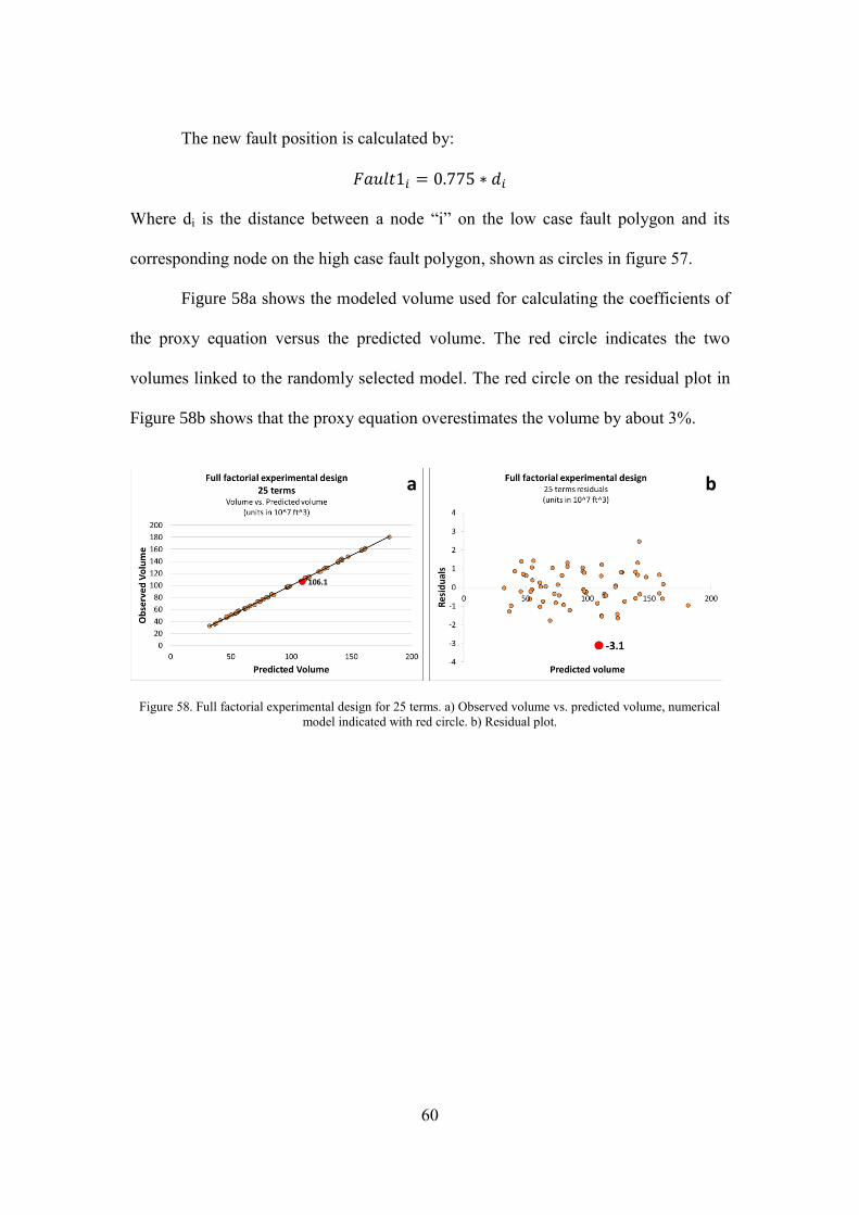
Figure 58a shows the modeled volume used for calculating the coefficients of

the proxy equation versus the predicted volume. The red circle indicates the two

volumes linked to the randomly selected model. The red circle on the residual plot in

Figure 58b shows that the proxy equation overestimates the volume by about 3%.

Figure 58. Full factorial experimental design for 25 terms. a) Observed volume vs. predicted volume, numerical

model indicated with red circle. b) Residual plot.

a b

61

5. Discussion

5.1 UNCERTAINTY IN STRATIGRAPHIC HORIZONS

All uncertainties related to stratigraphic horizons in this study are quantitative

and represented by a Gaussian distribution. The benefit of using a Gaussian

distribution for describing the uncertainties is that if the mean and standard deviation

are known, it is possible to compute the percentile rank associated with any given

score. In other words, the standard deviation delivers the criteria for deriving the high

and low case model parameters.

One source of the seismic uncertainties affecting the stratigraphic horizons is

time migration, where seismic events are relocated to the location the event occurred

in the subsurface. Time migration is not working accurately in case of strong lateral

velocity variations (Hubral et al., 1980). This may be the case for instance due to

major velocity boundaries with a steep slope. Another source of uncertainty is static

problems, which appear as amplitude variations between traces. At sea, the water is

homogeneous and static problems are minimal, unless the ocean floor is irregular

(Pritchett, 1990). Structural smoothing solves the static problem. However, this

process has the unwanted side effect of smoothing out real properties. This type of

uncertainty can be thought of as noise in the natural system. A difference map of the

original seismic volume and a smoothed volume shows that uncertainties due to

statics have a Gaussian distribution and account for ± 1.32 ms, and therefore their

impact is insignificant for the uncertainty study (see Figure 35).

The structural geometries of the reservoir limit the influence of the top

reservoir location. The reservoir shows a steep slope and consequently the OWC cuts

62

the reservoir under a relative steep angle. A considerable part of the reservoir base is

above the OWC as well. Therefore, a change of the top reservoir position in time has

only a limited effect on the reservoir volume. Separating the uncertainties of the

overburden and the reservoir units by stacking thickness maps below the top reservoir

allows the analysis of the reservoir thickness uncertainty. For an average thickness of

24 ms, the thickness error standard deviation of 6.5 ms is about 27% of the reservoir

thickness. This explains why the reservoir thickness uncertainty has a dominant

influence on the reservoir volume uncertainty (see Figure 53).

5.2 UNCERTAINTY IN FAULT POSITION

The influence of the fault uncertainty on the reservoir volume depends on the

relationship between the volume covered by the fault zone within the reservoir and

the reservoir volume. There is significant subjectivity involved in deriving the

envelope of the fault zones. In this thesis, the envelope is described by the high and

low case fault positions from interpreted fault polygons on ant tracking time slices.

Each polygon set was densely sampled and a new node drawn half the distance

between each node on the high and low case fault polygon to represent the base case

fault position. A more accurate method would be to define a rotation matrix for the

fault object in strike direction and compute the true stratigraphic thickness between

the extreme cases. This method more accurately derives the fault geometry while

honoring the full extent of the uncertainty envelope defined by the extreme cases.

63

5.3 UNCERTAINTY IN DEPTH CONVERSION

The choice of gridding algorithm (moving average) interpolates the V0 to an

average value outside the influence radius of the wells; subsequently this method has

relatively small deviations of depth errors compared to other gridding methods that

use the slope of the data points (see Table 4). The blind well test delivers a standard

deviation of 7.84 ft, which is about 0.12% of the average depth. Small deviations in

the depth thickness uncertainty are observable. The reservoir thickness depth error

distribution delivers a standard deviation of 12.05 ft. This is about 12% of the average

thickness. Consequently, its influence on the reservoir volume is not dramatic.

Similarly, as explained in section 5.1, the amount of volume translated above

and below the OWC due to depth conversion depends on the structural geometry of

the reservoir. This explains why the depth conversion has such a low impact on the

reservoir volume for a thin, dipping reservoir. As the result, if the reservoir would not

show a significant slope the depth conversion probably has a larger impact where it

would be divided horizontally into an oil zone at the top and a water zone at the base.

5.4 EXPERIMENTAL DESIGN

A key benefit of experimental design is that it works with extreme cases of the

parameter values, rather than stochastic simulation.

For example, the uncertainty in reservoir thickness can be modelled by

stochastically simulating an error surface and adding it to the thickness. A stochastic

simulation of an error surface produces many surfaces that have the same properties

controlled by a random number generator. The simulation of the error surface depends

not only on the standard deviation but also on a couple of simulation parameters, i.e.

64

the variogram parameters. As these parameters are subject to uncertainty, addressing

the uncertainty stochastically becomes complicated. When working with experimental

design and low, base and high cases for each parameter the volume uncertainty

estimation becomes simpler and easier to quality check. In addition, any combination

of parameter values used by the proxy equation is reproducible as a numerical model.

65

6. Conclusion

Uncertainty is a well-known concept in geology, and can lead to reevaluation

of important development decisions if properly assessed. A general method of

handling uncertainty is by describing it in the form of a probability density function or

a cumulative distribution function.

This thesis provides a robust methodology for capturing the structural

uncertainty and its impact on the volumetrics. Key elements of this method are using

Gaussian error distributions for defining the low and high case for the reservoir

parameters. In addition, a novel method based on volumetric seismic attributes was

introduced for capturing the fault uncertainty. Finally, a method was developed that

allows to extract the modeling parameters from any parameter setting of the proxy

equation describing the reservoir volume. This study has shown that a small variation

in a reservoir parameter can mean a significant change in reservoir volume.

The main sources of uncertainty lie within the data source used for structural

modeling. The quality of seismic reflection surveys is highly dependent on acquisition

and processing. Volume attributes can improve the signal to noise ratio or enhance

structural features, where the seismic resolution is an issue, thus making the

interpretation more reliable.

One interesting result is that the uncertainties in the seismic picks and

consequently in the reservoir thickness have a much greater impact on the gross-

volume compared to the influence of faults and velocity uncertainties. The

uncertainties in the top reservoir in the time and depth domain have only a moderate

influence on the volume uncertainty, which is related to the structural geometries of

66

the reservoir. The constant interval velocity used for the depth thickness uncertainty is

a good approximation of the interval velocities of the reservoir. This indicates that the

interval velocities of the reservoir do not change significantly, consequently resulting

in minor uncertainty in the depth thickness. The uncertainty of the fault position

would also have a greater influence on the volume uncertainty if the reservoir area is

small and the fault displacement uncertainty relatively large. This study shows that

seismic uncertainties in the reservoir thickness have a larger impact on thin reservoirs.

The limitation of the described method is that it requires a sufficient amount of

drilled wells in order to derive meaningful error distributions. Sufficient well data is

not always available at the development stage. In addition, different tectonic settings

introduce new parameters to the uncertainty analysis, where the reservoir drapes onto

a salt dome for instance or along a convergent plate boundary. Thus, a wider range of

structurally complex models involving a large number of parameters should be

evaluated.

References

Bárdossy, G., & Fodor, J. (2001). Traditional and new ways to handle uncertainty in

geology. Natural Resources Research, 10(3), 179-187.

Bascle, B. J., Nixon, L. D., & Ross, K. M. (2001). Atlas of Gulf of Mexico Gas and

Oil Sands as of January 1, 1999: Minerals Management Service, Gulf of

Mexico OCS Region, Office of Resource Evaluation.

Bird, D. E., Burke, K., Hall, S. A., & Casey, J. F. (2005). Gulf of Mexico tectonic

history: Hotspot tracks, crustal boundaries, and early salt distribution. AAPG

bulletin, 89(3), 311-328.

Caers, J. (2005). Petroleum geostatistics: Richardson, TX: Society of Petroleum

Engineers.

Caers, J. (2011). Modeling uncertainty in the earth sciences. Chichester: Wiley-

Blackwell.

67

Galloway, W. E. (2008). Depositional evolution of the Gulf of Mexico sedimentary

basin. Sedimentary basins of the world, 5, 505-549.

Hart, B. S. (2011). Structural Interpretation An Introduction to Seismic Interpretation

(pp. 42): AAPG.

Hubral, P., Krey, T., & Larner, K. L. (1980). Interval velocities from seismic

reflection time measurements: Society of Exploration Geophysicists Tulsa.

Lecour, M., Cognot, R., Duvinage, I., Thore, P., & Dulac, J. C. (2001). Modelling of

stochastic faults and fault networks in a structural uncertainty study.

Petroleum Geoscience, 7(4 SPEC. ISS.), 31-42.

Mann, C. J. (1993). Uncertainty in geology. Computers in Geology–25 Years of

Progress, Oxford University Press, Oxford, 241-254.

Osypov, K., Nichols, D., Woodward, M., Zdraveva, O., Qiao, F., Yarman, E.,

Ivanova, N. (2011). From quantifying seismic uncertainty to assessing E&P

risks and the value of information. Paper presented at the 2011 SEG Annual

Meeting.

Plackett, R. L., & Burman, J. P. (1946). The design of optimum multifactorial

experiments. Biometrika, 305-325.

Pritchett, W. C. (1990). Acquiring better seismic data: Springer Science & Business

Media.

Røe, P., Georgsen, F., & Abrahamsen, P. (2014). An Uncertainty Model for Fault

Shape and Location. Mathematical Geosciences, 46(8), 957-969.

Samson, P., Dubrule, O., & Euler, N. (1996). Quantifying the impact of structural

uncertainties on gross-rock volume estimates. Paper presented at the NPF/SPE

European 3-D Reservoir Modelling Conference.

Schlumberger, 2009, Petrel manual: Velocity Modeling Course: Schlumberger

Schlumberger, 2010, Petrel manual: Interpreter’s Guide to Seismic Attributes:

Schlumberger

Srivastava, R. M. (1992). Reservoir characterization with probability field simulation.

Paper presented at the Proceedings - SPE Annual Technical Conference and

Exhibition.

68

Steppan, D. D., Werner, J., & Yeater, R. (1998). Essential regression and

experimental design for chemists and engineers. MS excel add in software

package, 2001.

Thore, P., Shtuka, A., Lecour, M., Ait-Ettajer, T., & Cognot, R. (2002). Structural

uncertainties: Determination, management, and applications. Geophysics,

67(3), 840-852.

Vincent, G., Corre, B., & Thore, P. (1999). Managing structural uncertainty in a

mature field for optimal well placement. SPE Reservoir Evaluation and

Engineering, 2(4), 377-384.