Math 256 - Applied Differential Equations Notes

Existence and Uniqueness

The following theorem gives sufficient conditions for the existence and uniqueness of a solu-tion to the IVP for first order nonlinear o.d.e. We omit the proof as it is beyond the scopeof this class.

Proposition: If f(x, y) is cont. on the open rectangle R = {(x, y)|a < x < b, c < y < d}that contains (x0, y0) then the IVP y′ = f(x, y), y(x0) = y0 has a solution on some openinterval contained in (a, b) that contains x0. If the partial fy is also continuous on R thenthe IVP has a unique solution.

Consider the IVP y′ = 2x 3√y, y(x0) = y0. For what points (x0, y0) does this IVP have

a solution? For what points (x0, y0) does this IVP have a unique solution (on some openinterval containing x0)?

Since f(x, y) = 2x 3√y is continuous for all points in the xy-plane, there exists a solution to

the IVP for any point (x0, y0).

fy(x, y) =2x

3 3√y2

is continuous everywhere except where y = 0. So for any (x0, y0) such that

y0 6= 0 there is an open rectangle R on which both f and fy are continuous, and hence thereis a unique solution to the IVP on some open interval containing x0.

y′ = 2x 3√y, y(0) = 0 has at least two solutions on any interval containing 0:

y = 0 and y =

√8

27x3.

Why didn’t we get a unique solution on some interval containing 0?

Because for f(x, y) = 2x 3√y, the partial fy =

2x

3 3√y2

isn’t continuous at y = 0.

Transformations of Nonlinear o.d.e.

Sometimes a nonlinear first order o.d.e. isn’t separable, but can be “transformed” into aseparable equation by having y = uy1 where y1 is a suitably chosen known function, and usatisfies a separable equation.

A special kind of non-linear first order o.d.e. is an equation of the form y′ + p(x)y = f(x)yr

where r is any real other than 0 or 1 (the only values of the r that actually make the o.d.e.linear). Such an o.d.e. is called a Bernoulli equation. If r > 0 then y = 0 is a solution to aBernoulli equation.

Suppose y1 is a non-trivial solution to the complementary equation y′ + p(x)y = 0. Let’ssubstitute y = uy1 where u is a function of x to see how that transforms the equation:

y′ + p(x)y = f(x)yr becomes u′y1 + uy′1 + p(x)uy1 = f(x)(uy1)r.

Since this can be rewritten as u′y1 + u(y′1 + p(x)y1) = f(x)(uy1)r and y′1 + p(x)y1 = 0 we get

u′y1 = f(x)uryr1.

This transformed equation is separable!

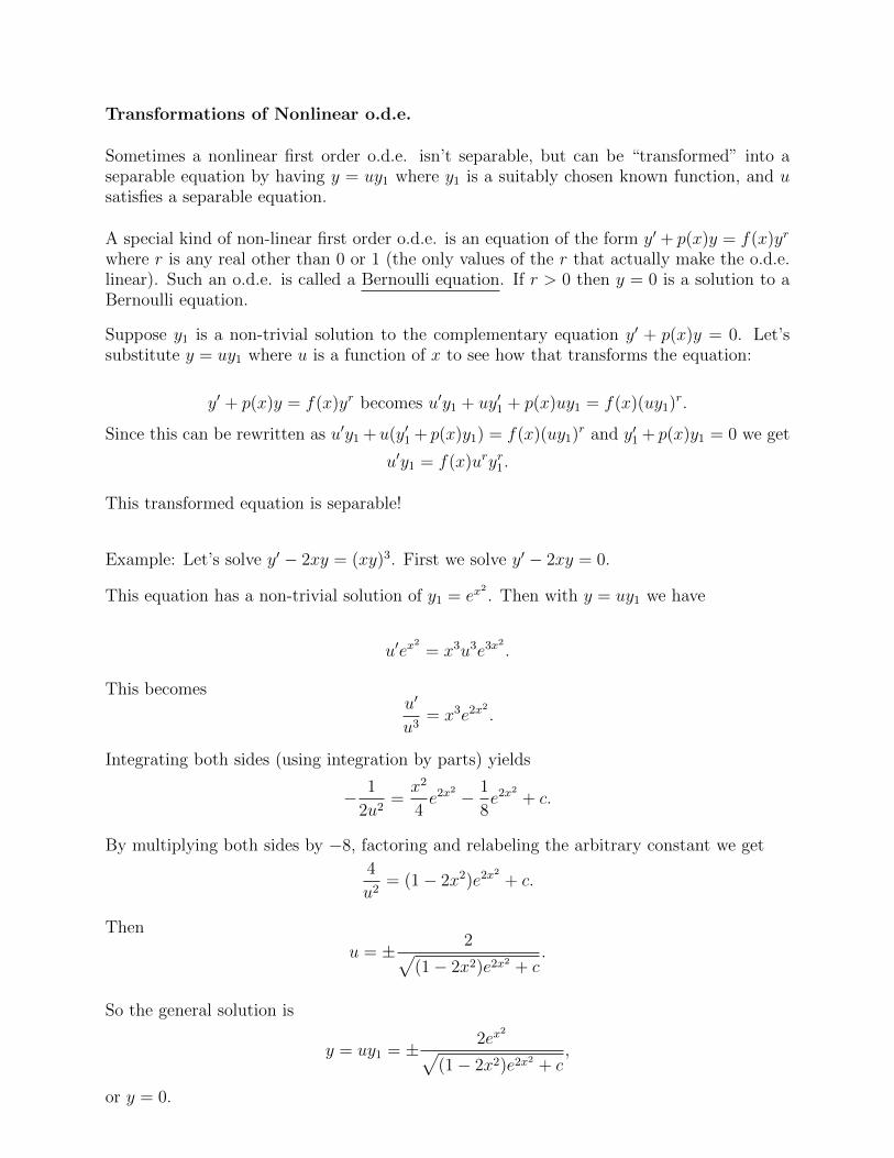
Example: Let’s solve y′ − 2xy = (xy)3. First we solve y′ − 2xy = 0.

This equation has a non-trivial solution of y1 = ex2. Then with y = uy1 we have

u′ex2

= x3u3e3x2

.

This becomesu′

u3= x3e2x

2

.

Integrating both sides (using integration by parts) yields

− 1

2u2=x2

4e2x

2 − 1

8e2x

2

+ c.

By multiplying both sides by −8, factoring and relabeling the arbitrary constant we get

4

u2= (1− 2x2)e2x

2

+ c.

Then

u = ± 2√(1− 2x2)e2x2 + c

.

So the general solution is

y = uy1 = ± 2ex2√

(1− 2x2)e2x2 + c,

or y = 0.

Consider a non-linear first order o.d.e. y′ = f(x, y). Suppose x, y occur in f(x, y) in such away that y′ = q(y/x) where q(u) is a function of a single variable. In this case the o.d.e. issaid to be nonlinear homogeneous.

Consider the non-linear first order o.d.e. y′ =y − x sec

(yx

)x

. It’s (nonlinear) homogeneous

since it can be rewritten asy′ =

y

x− sec

(yx

),

which is of the form y′ = q(y/x) for q(u) = u− sec (u).

Here is the transformation: Substitute y = ux into the equation y′ = q(u) to get

u′x+ u = q(u).

This is separable (ignoring the constant solution u = u0 where q(u0) = u0) as it can berewritten as

u′

q(u)− u=

1

xon an interval not containing x = 0.

Let’s apply this to y′ = q(u) = u− sec (u). This yields

− cos (u)u′ =1

x.

Then

−∫

cos (u) du = ln |x|.

This becomes− sin (u) = ln |x|+ c.

Hence (relabeling the constant) u = sin−1 (c− ln |x|) and therefore

y = ux = x sin−1 (c− ln |x|).

Now consider the IVP with this o.d.e. and the initial condition y(e) = 0. By imposing theinitial condition, we get c = 1, so the IVP has the solution

y = x sin−1 (1− ln (x)).

Exact Equations

A convenient way to write a first order o.d.e. is with differentials:

M(x, y) dx+N(x, y) dy = 0.

This is equivalent to M(x, y) +N(x, y)y′ = 0 for y is a function of x.

We will say that F (x, y) = c is an implicit solution of M(x, y) dx + N(x, y) dy = 0 if everydifferentiable function y(x) such that F (x, y(x)) = c is a solution of M(x, y)+N(x, y)y′ = 0.

Let’s show that x2y + 2xy3 = c is an implicit solution of 2y(x+ y2) dx+ x(x+ 6y2) dy = 0.By implicit differentiation, regarding y as a function of x,

2xy + x2y′ + 2y3 + 6xy2y′ = 0→

2y(x+ y2) + x(x+ 6y2)y′ = 0.

More generally, F (x, y) = c is an implicit solution of Fx dx+ Fy dy = 0 where Fx, Fy denotethe x, y partials respectively.

This motivates the following important definition:

M(x, y) dx + N(x, y) dy = 0 is exact on an open rectangle R if there is a function F (x, y)such that Fx, Fy are continuous on R, and

Fx(x, y) = M(x, y) and Fy(x, y) = N(x, y),

for all (x, y) in R.

It turns out (we skip the proof) that M(x, y) dx+N(x, y) dy = 0 is exact on an open rectangleR if and only if My = Nx (assuming My, Nx are continuous on R).

An implicit solution for an exact equation M(x, y) dx+N(x, y) dy = 0 is straightforward:

Integrate M with respect to x, producing a constant of integration that can be a functionof y. Then take the y-partial of the result to determine the constant of integration.

Note: One can do the above with the roles of M and N switched and the roles of x and yswitched.

This gives F (x, y) and an implicit solution of F (x, y) = c. If possible, find an explicit solutiony(x) from F (x, y) = c.

Determine if the equation is exact, and if so, solve it:

(1) (2xy + 3x2) dx+ (x2 + cos (y)) dy = 0.

The y-partial of M(x, y) = 2xy + 3x2 is My = 2x.

The x-partial of N(x, y) = x2 + cos (y) is Nx = 2x.

Since My = Nx everywhere in the xy-plane, this equation is exact (on any openrectangle).

By integrating M with respect to x we get F (x, y) = x2y + x3 + g(y). By takingthe y-partial we get Fy = x2 + g′(y). So g′(y) = cos (y) and hence g(y) = sin (y)works (we may set the constant of integration to 0).

Therefore, x2y + x3 + sin (y) = c is an implicit solution.

(2) (y3 − 1)ex dx+ 3y2(ex + 1) dy = 0.

The y-partial of M(x, y) = (y3 − 1)ex is My = 3y2ex.

The x-partial of N(x, y) = 3y2(ex + 1) is Nx = 3y2ex.

Since My = Nx everywhere in the xy-plane, this equation is exact (on any openrectangle).

Integrating M with respect to x yields F (x, y) = (y3 − 1)ex + g(y). Then Fy =3y2ex + g′(y). We want g′(y) = 3y2. So set g(y) = y3.

Thus, (y3 − 1)ex + y3 = c is an implicit solution. We can take this one further!

This implicit solution is equivalent to y3(ex+1) = ex+c and therefore, y = 3

√ex + c

ex + 1is the explicit general solution.

(3) 3x2y2 dx+ 4x3y dy = 0.

The y-partial of M(x, y) = 3x2y2 is My = 6x2y and the x-partial of N(x, y) = 4x3yis Nx = 12x2y.

Except for on the x- or y-axis, My 6= Nx. Hence there is no open rectangle onwhich this equation is exact.

Now suppose M(x, y) dx+N(x, y) dy = 0 is not exact, but can be made exact by multiplyingboth sides by some function µ(x, y). Such a function is called an integrating factor.

Of course we have seen this terminology already:

The equation y′ + p(x)y = f(x) can be rewritten as dy + (p(x)y − f(x)) dx = 0. Thenµ = e

∫p(x) dx is an integrating factor since µ dy + (µp(x)y − µf(x)) dx = 0 is exact as

∂

∂x(µ) = p(x) =

∂

∂y(µp(x)− µf(x)) .

Consider the o.d.e.

(3x+ 2 +

2

y

)dx+

(x2 + x

y

)dy = 0.

With M = 3x+ 2 +2

yand N =

x2 + x

ywe get My = − 2

y2and Nx =

2x+ 1

y, so the equation

isn’t exact.

Multiplying both sides by µ(x, y) = xy we get (3x2y + 2xy + 2x) dx+ (x3 + x2) dy = 0.

This equation is exact since for M = 3x2y + 2xy + 2x and N = x3 + x2 we get

My = 3x2 + 2x = Nx.

Now we can solve as before:

Taking the integral of N = x3 + x2 with respect to y yields x3y + x2y + g(x). Taking thex-partial and equating with M = 3x2y + 2xy + 2x implies that we may set g(x) = x2.

So an implicit solution is x3y + x2y + x2 = c which we can solve for y to get the explicitsolution:

y =c− x2

x3 + x2.

Let’s consider how to find an integrating factor in a special case:

Proposition: Let M,N,My, Nx be continuous functions on an open rectangle R in thexy-plane. Assume that p = (My −Nx)/N is independent of y. Then

µ(x) = ±e∫p(x) dx

is an integrating factor of M dx+N dy = 0 on R.

Proof : (µM)y = µyM + µMy = µMy = µ(pN +Nx).

(µN)x = µxN + µNx = µpN + µNx = (µM)y.

Hence µM dx+ µN dy = 0 is exact �

Example: Let’s solve (2xy + x + 3y) dx + (2x + 1) dy = 0. This equation isn’t exact as forM = 2xy + x+ 3y and N = 2x+ 1 we have My = 2x+ 3 and Nx = 2 which aren’t equal.

p = (My − Nx)/N = (2x + 1)/(2x + 1) = 1 is independent of y. So we get an integratingfactor:

µ = e∫p(x) dx = ex.

Now consider the equation ex(2xy+x+3y) dx+ex(2x+1) dy = 0. Integrating N = ex(2x+1)with respect to y yields

yex(2x+ 1) + g(x).

Differentiating this with respect to x gives

y(ex(2x+ 1) + 2ex) + g′(x) = yex(2x+ 3) + g′(x).

Setting this equal to ex(2xy + x+ 3y) tells us that g′(x) = xex.

By integrating by parts we can set g(x) = xex − ex. So (2x + 1)exy + xex − ex = c is animplicit solution of (2xy + x+ 3y) dx+ (2x+ 1) dy = 0.

We can solve for the explicit solution:

y =ce−x − x+ 1

2x+ 1.

Consider the IVP

(tan−1 (y)

x+ 2

)dx+

1

1 + y2dy = 0, y(1) = 0.

For M =tan−1 (y)

x+ 2 and N =

1

1 + y2we have My =

1

x(1 + y2)and Nx = 0.

So the equation isn’t exact.

But (My −Nx)/N =1

xis independent of y. This yields an integrating factor of

µ = ±e∫

1xdx = ±eln |x| = ±x.

So let’s solve(tan−1 (y) + 2x

)dx+

x

1 + y2dy = 0.

By integratingx

1 + y2with respect to y we get x tan−1 (y) + g(x). The x-partial of this is

tan−1 (y) + g′(x). Setting this equal to tan−1 (y) + 2x tells us we can set g(x) = x2.

Thus x tan−1 (y)+x2 = c is an implicit solution, which can be solved for the explicit solution:

y = tan

(c− x2

x

).

Finally, let’s impose the initial condition y(1) = 0:

0 = tan (c− 1)→ c− 1 = 0→ c = 1.

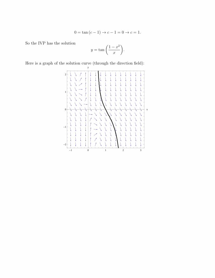
So the IVP has the solution

y = tan

(1− x2

x

).

Here is a graph of the solution curve (through the direction field):

-1 0 1 2 3

-2

-1

0

1

2

x

y

Autonomous First Order Equations

Note: This material is not covered in the textbook.

A first order differential equation of the formdy

dt= f(y) is said to be autonomous.

The rate function f does not depend on the independent variable t.

Here are a few useful properties of first order autonomous differential equations

(1) They are separable.(2) The slopes in the direction field only depend on y.(3) The general solution is invariant under horizontal translations.

Example: Exponential growth or decay.

Let q(t) be the quantity of something. This common model assumes that the rate of growthin q is proportional to itself:

dq

dt= rq.

Examples include population growth (r > 0) and radioactive decay (r < 0). As we havealready seen, with an initial condition q(t0) = q0, we have q(t) = q0e

r(t−t0).

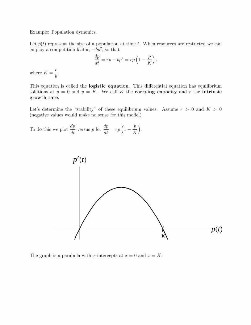
Example: Population dynamics.

Let p(t) represent the size of a population at time t. When resources are restricted we canemploy a competition factor, −bp2, so that

dp

dt= rp− bp2 = rp

(1− p

K

),

where K =r

b.

This equation is called the logistic equation. This differential equation has equilibriumsolutions at y = 0 and y = K. We call K the carrying capacity and r the intrinsicgrowth rate.

Let’s determine the “stability” of these equilibrium values. Assume r > 0 and K > 0(negative values would make no sense for this model).

To do this we plotdp

dtversus p for

dp

dt= rp

(1− p

K

):

KpHtL

p¢HtL

The graph is a parabola with x-intercepts at x = 0 and x = K.

Note:

If 0 < p < K thendp

dt> 0 and p is increasing. If p > K then

dp

dt< 0 and p is decreasing. So

if p is close to K then p is “pushed” towards K. A similar analysis shows that if p is closeto 0 it will be “pushed” away from 0.

(While we getdp

dt< 0 when p < 0, it’s not relevant to the model as p cannot be nega-

tive.)

We can use arrows to indicate how p is “pushed.” Here it is with the logistic equation:

K0pHtL

p¢HtL

The solution p = K is an asymptotically stable equilibrium solution, since smallperturbations (changes) are “pushed” back towards K. The solution p = 0 is an unstablesolution, since any perturbations will “push” p away from 0.

With the arrows, the p-axis is called the phase line.

More Examples:

Find and classify the equilibrium solutions ofdy

dt= (1− y)(2− y).

1 2yHtL

y¢HtL

The equilibrium solutions are y = 1 and y = 2. Since y′ is positive outside of the interval[1, 2] and negative inside (1, 2), y = 1 is an asymptotically stable solution and y = 2 is anunstable solution

Find and classify the equilibrium solutions ofdy

dt= y(2− y)2.

0 2yHtL

y¢HtL

The equilibrium solutions are y = 0 and y = 2. y = 0 is an unstable solution and y = 2 is asemistable equilibrium solution since it is stable from one side (in this case from below)while unstable from the other side (in this case from above).

Find and classify the equilibrium solutions ofdy

dt= sin(y).

-Π 0 Π 2Π 3ΠyHtL

y¢HtL

Unstable equilibria exist at t = 0,±2π,±4π, ...

Stable equilibria exist at t = ±π,±3π, ...

Applications of First Order o.d.e.

We start with the classic exponential model : y′(t) = ky, y(t0) = y0.

The general solution (without an initial value) is y(t) = cekt. If k > 0 the model is calledexponential growth and if k < 0 the model is called exponential decay. The constant k iscalled a growth constant and decay constant respectively.

Applying the initial value, y0 = cekt0 , so c = y0e−kt0 . The initial value problem has the

solutiony = y0e

k(t−t0).

We assume that you have seen examples (in algebra and calculus) of using the exponentialmodel to model at least population growth, compound interest, and radioactive decay (usingthe half-life).

Let’s consider a variation on the exponential model:

Suppose that a radioactive substance has decay constant k > 0 (reported as a positivenumber, so use y′ = −ky). At the same time the substance is being produced at a constantrate of a units of mass per unit time.

Let y(t) be the amount of the substance at time t and y(0) = y0 be the initial mass. Let’sderive an IVP and solve it. Then we can take the limit of y(t) as t → ∞ to find theequilibrium solution.

First we derive a differential equation: y′(t) = the rate of increase in y(t) − the rate of decrease in y.

So y′(t) = a − ky. We can solve this in various ways. Since it’s separable let’s solve it byintegrating.

1

a− kyy′ = 1→ −1

kln |a− ky| = t+ c→ a− ky = ce−kt → y =

a

k+ ce−kt.

Imposing the initial condition we get:

y0 =a

k+ c→ c = y0 −

a

k.

So the solution to the IVP isy =

a

k+(y0 −

a

k

)e−kt.

The equilibrium solution is y =a

k. In particular, if y0 > a/k then y decreases toward this

solution, and if y0 < a/k then y increases towards this solution.

A mixing problem:

An immortal alchemist creates bitcoin at the rate of 1 bitcoin per day. Going unnoticed, ahacker has written code that is continuously stealing it at a rate that is equivalent, on a dailybasis, to 2.5 percent of whatever is there. What is the number of bitcoins b(t) the alchemisthas at time t? Assume b(0) = 1. How many bitcoins will the alchemist have in the long run(as t→∞)?

b′(t) = rate of increase in bitcoin − rate of decrease in bitcoin.

So b′ = 1− 0.025b. Using a = 1, k = 0.025, and b0 = 1 we get b(t) = 40− 39e−0.03t.

In the long run the alchemist will have 40 bitcoins.

Newton’s Law of Cooling:

If an object of temperature T (t) at time t is in a medium of temperature Tm(t) at time t thenthe rate of change in T (t) is proportional to the ∆T = T (t)−Tm(t). When T (t) > Tm(t) wehave T ′(t) < 0 and when T (t) < Tm(t) we have T ′(t) > 0.

So T (t) satisfies T ′ = −k(T − Tm) where k > 0.

Suppose a cup of coffee brewed at 150 degrees Fahrenheit is cooling in a room of constanttemperature 70 degrees Fahrenheit. After 10 minutes the temperature of the coffee is 100degrees Fahrenheit. How hot is the temperature after 20 minutes?

First we setup the IVP: T ′ = −k(T − 70), T (0) = 150.

Then ln |T − 70| = −kt + c implies T − 70 = ce−kt and hence T = 70 + ce−kt. By imposingthe initial condition, T (t) = 70 + 80e−kt.

Since we are given T (10) = 100 we can solve for k:

100 = 70 + 80e−10k → k = −0.1 ln (3/8) = ln (8/3)/10

Then after 20 minutes the cup of coffee is at T (20) = 70+80e−2 ln (8/3) = 70+80(9/64) = 81.25degrees Fahrenheit.

Another mixing problem:

A tank initially contains 10 kg of salt dissolved in 200 L of water. Brine that contains 0.5 kgof salt per liter is pumped into the tank at 5 liters per minute and at the same time wateris drained from the tank at 5 liters per minute. Assume the tank is always kept uniformlymixed. Calculate the amount of salt in the tank in the long run (the equilibrium solution ast→∞).

Let’s pose this as an IVP: Let y(t) be the amount of salt in kg in the tank (which alwayscontains 200 L of water).

Then y′ = rate of salt in − rate of salt out.

So

y′ =

(0.5 kg

L

)(5 L

min

)−(y(t) kg

200 L

)(5 L

min

), y(0) = 10.

Again, we can solve y′ = 2.5− y/40 in more than one way, but it is separable:

1

2.5− y/40y′ = 1→ −40 ln |2.5− y/40| = t+ c→ 2.5− y/40 = ce−t/40 → y = 100 + ce−t/40.

Imposing the initial condition yields c = −90, so y = 100 − 90e−t/40. Thus as t → ∞,y → 100. So in the long run the amount of salt in the tank is 100 kg.

Here is a variation on the problem above:

A tank of maximum capacity 1, 000 gallons initially contains 10 lb of salt dissolved in 500gallons of water. Brine that contains 0.5 lb of salt per gallon is pumped into the tank at10 gallons per minute and at the same time water is drained from the tank at 5 gallons perminute. Assume the tank is always kept uniformly mixed. Calculate the amount of salt inthe tank the moment it begins to overflow.

The change here is the amount of water in the tank at time t isn’t constant: V (t) = 500 + 5tis the volume of the tank in gallons after t minutes where V (0) = 500.

We still set it up like before: Let y(t) be the amount of salt in the tank in lb at time t, wherey(0) = 10.

Then y′ = rate of salt in − rate of salt out.

So

y′ =

(0.5 lb

gal

)(10 gal

min

)−(

y(t) lb

500 + 5t gal

)(5 gal

min

), y(0) = 10.

So we have to solve the following IVP: y′ = 5− 1

100 + ty, y(0) = 10.

Let’s rewrite the o.d.e. as y′ +1

100 + ty = 5. An integrating factor is found by computing

µ = e∫

1100+t

dt = eln |100+t| = ±(100 + t).

Let’s multiply both sides of the o.d.e. by 100 + t:

(100 + t)y′ + y = 5(100 + t).

This becomes((100 + t)y)′ = 5(100 + t).

Integrating both sides yields

(100 + t)y = 5(100t+ 0.5t2) + c→ y =500t+ 2.5t2 + c

100 + t.

By imposing the initial condition y(0) = 10 we get 10 =c

100, so c = 1, 000. So

y =1, 000 + 500t+ 2.5t2

100 + t.

Now to find the amount of salt at the moment the tank overflows: Set V (t) = 500+5t = 1, 000to get t = 100 minutes.

Then y(100) = 380 lbs of salt when the tank overflows.

Motion with resistance: We assume an object is traveling vertically through a medium (air orwater for example) and that the only forces acting on the object are a constant gravitationalforce pulling the object down and the resistance of the medium (directly proportional to thespeed of the object).

Suppose an object of mass m > 0 moves through vertically a medium under a constantdownward gravitational force Fg = mg (where g is the constant acceleration due to gravity)and the medium exerts a force of Fmed = k|v|, k > 0, in the opposite direction of the motion,where v is the velocity of the object.

Let’s derive a model for this scenario:

Let v be the vertical velocity of an object . Then Newton’s second law of motion assertsthat Fnet = ma where a = v′.

Suppose the object is moving up. Then the resistance acts downward: Fmed = −k|v| = −kv.Now suppose the object is moving down. Then the resistance acts upward: Fmed = k|v| =k(−v) = −kv.

Either way, the net force on the object is and Fnet = −mg − kv.

So we get the following first order linear o.d.e. mv′ = −mg − kv.

This can be expressed as v′ +k

mv = −g.

While this is separable, we can solve quickly it by finding an integrating factor: µ = e(k/m)t.

e(k/m)tv′ +k

m= −ge(k/m)t → (e(k/m)tv)′ = −ge(k/m)t → e(k/m)tv = −mg

ke(k/m)t + c.

(ELFY) Solve it as a separable ode by separating the variables and integrating both sides.

Hencev(t) = −mg

k+ ce−(k/m)t.

Finally, we see that limt→∞

v(t) = −mgk

is the equilibrium solution, which is called the

terminal velocity in this context.

Given an initial value v0 for the velocity, we get c = v0 + mgk

.

A 4 kg object is launched vertically into the air at 40 meters per second near the surfaceof the Earth (we assume far enough up that the object will attain terminal velocity beforereaching the surface of the Earth).

Suppose the air resists motion with a force of 4.9 Newtons for each m/s of speed. Usingg = 9.8 meters per square second, find a model for the objects vertical velocity and find theterminal velocity.

We can just plug-in to the general model we just derived: v(t) = −4(9.8)4.9

+(40+ 4(9.8)4.9

)e−(4.9/4)t.

So v(t) = −8 + 48e−(49/40)t.

The terminal velocity is −8. Meaning that in the end the object falls at a constant rate of8 meters per second.

[IF TIME PERMITS COVER 2ND ORDER AUTONOMOUS AND ESCAPE VELOCITY]

A Brief Treatment of Second Order Autonomous

A second order equation is autonomous if it can expressed in the form y′′ = F (y, y′). Theindependent variable (x or t) does not appear in the differential equation. We will use t forthe independent varible.

Let v = y′. By the Chain Rule we can write that y′′ = v′ =dv

dt=dv

dy

dy

dt=dv

dyy′ =

dv

dtv.

So the second order autonomous equation y′′ = F (y, y′) reduces to the first order equation

vdv

dy= F (y, v), where we treat y as the independent variable in v. We will only look at some

very basic examples, ones where y′′ = p(y).

Consider the equation y′′ + y = 0. By letting v = y′, this equation reduces to vdv

dy+ y = 0,

which is separable. The reader is left to check that we do indeed get

v = ±√C − y2, where C ≥ 0.

If we plot these curves (for various values of C) in the (y, v)-plane (a so-called “Poincarephase plane) we get a bunch of circles. On one circle we see that if |y| is larger, |v| is smallerand vice versa (going around clockwise). This represents oscillations!

(Exercise left for you!) Find y(t) given that it satisfies y′ = v = ±√R2 − y2. Confirm the

oscillations?

In general, finding y(t) from v(y) just requires solving a separable equation, which is some-thing we know how to do, but often it is really quite hard because of the integration required.

Let’s return to y′′ + y = 0. Notice that if y = 0 then y′ = 0 and so y = 0 is a constantsolution (equilibrium of the second order autonomous equation)!

The corresponding point (0, 0) in the Poincare phase plane (horizontal y-axis, vertical v axis)is called a critical point. Such a equilibrium is stable if small perturbations in either y tendto keep the values of y and y′ relatively “near” to the critical point (y equal to the constant,v = y′ equal to 0). Otherwise it’s unstable.

In the case of y = 0 in y′′ + y = 0, it’s stable since small perturbations move to a circulartrajectory near to and about the origin.

Consider y′′ + sin (y) = 0. It has equilibria at y = nπ where n is an arbitrary integer.

The equation reduces to vdv

dy+ sin (y) = 0, which is separable. The reader is left to check

that we do indeed getv2 = 2 cos (y) + C.

Consider the equilibrium y = nπ where n is an even integer (i.e. y = 0).

vdv

dy= − sin (y). If y is increased a little (so v > 0) then v

dv

dy< 0 meaning v and

dv

dyhave

opposite signs. If y is decreased a little (so v < 0) then vdv

dy> 0 meaning v and

dv

dyhave the

same sign. Either way, it follows thatdv

dy< 0 and

dy

dv< 0 (Inverse Derivative Rule).

This means that y and v move in opposition. As y increases, v decreases, causing y toslow and then (after v becomes negative) decrease. As y decreases, v increases, causingthe decrease in y to slow and then (after v becomes positive) increase. This makes theseequilibria stable.

Consider the equilibrium y = nπ where n is an odd integer (i.e. y = π).

The exact opposite thing happens at these equilibria. y and v move in concert. As y increases,so does v > 0 only causing y to increase more. That makes these equilibria unstable.

Over large vertical distances, gravitational models assume that gravity is inversely propor-tional to the square of the distance from the center of the massive object (assumed to be asphere). This is an example of an inverse square law.

Assume a spacecraft launches from the surface of the Earth and exhausts its fuel as it reachesa height h that sufficiently large that atmospheric resistance is negligible and can be assumedto be effectively 0. Let t = 0 be this time (known as “burnout”) and consider that the forceof gravity on the spacecraft at altitude y ≥ h is

Fg = − c

(R + y)2where c is a constant R is the radius of the Earth.

Using Fg = −mg when y = 0 where g is the acceleration due to gravity on the surface of theEarth, we get −mg = − c

R2 , so c = mgR2.

Thus

Fg = − mgR2

(R + y)2.

Since Fg is assumed to be the only force acting on the spacecraft for t ≥ 0,

Fg = ma = my′′ = − mgR2

(R + y)2→

y′′ = − gR2

(R + y)2.

This equation is autonomous, so with v = y′ it reduces to vdv

dy= − gR2

(R + y)2.

Integrating both sides yields

0.5v2 =gR2

R + y+ c→ v =

√2gR2

R + y+ c.

Now suppose we have an initial velocity of v(h) = v0.

Then v20 =2gR2

R + h+ c.

So c = v20 −2gR2

R + hand hence

v =

√2gR2

R + y+ v20 −

2gR2

R + h.

If v0 ≥√

2gR2

R + hthen v ≥ 0 for all y ≥ h and the spacecraft continues on up into space!

The expression ve =

√2gR2

R + his called escape velocity.

We will show that if v0 < ve the spacecraft falls back to Earth:

If v0 < ve then v =

√2gR2

R + y+ v20 −

2gR2

R + h= 0 for y such that

2gR2

R + y+ v20 −

2gR2

R + h= 0,

which occurs at y =2gR2h+R(R + h)v20

2gR2 − (R + h)v20≥ h since

2gR2

R + y=

2gR2

R + h− v20 ≤

2gR2

R + h.