mathematica for rogawski's calculus 2nd editiionusers.rowan.edu/~hassen/mathematica/mathematica...

Mathematica® for Rogawski's

Calculus 2nd Edition 2010

Based on Mathematica Version 7

Abdul Hassen, Gary Itzkowitz, Hieu D. Nguyen, Jay Schiffman

W. H. Freeman and CompanyNew York

© Copyright 2010

2 Mathematica for Rogawski's Calculus 2nd Editiion.nb

Table of Contents

Chapter 1 Introduction

1.1 Getting Started

1.1.1 First-Time Users of Mathematica 7

1.1.2 Entering and Evaluating Input Commands

1.1.3 Documentation Center (Help Menu)

1.2 Mathematica's Conventions for Inputting Commands

1.2.1 Naming

1.2.2 Parentheses, Brackets, and Braces

1.2.3 Lists

1.2.4 Equal Signs

1.2.5 Referring to Previous Results

1.2.6 Commenting

1.3 Basic Calculator Operations

1.4 Functions

1.5 Palettes

1.6 Solving Equations

Chapter 2 Graphs, Limits, and Continuity of Functions

2.1 Plotting Graphs

2.1.1 Basic Plot

2.1.2 Plot Options

2.2 Limits

2.2.1 Evaluating Limits

2.2.2 Limits Involving Trigonometric Functions

2.2.3 Limits Involving Infinity

2.3 Continuity

Chapter 3. Differentiation

3.1 The Derivative

3.1.1 Slope of Tangent

Mathematica for Rogawski's Calculus 2nd Editiion.nb 3

3.1.2 Derivative as a Function

3.2 Higher-Order Derivatives

3.3 Chain Rule and Implicit Differentiation

3.4 Derivatives of Inverse, Exponential and Logarithmic Functions

3.4.1 Inverse of a Function

3.4.2 Exponential and Logarithmic Functions

Chapter 4 Applications of the Derivative

4.1 Related Rates

4.2 Extrema

4.3 Optimization

4.3.1 Traffic Flow

4.3.2 Minimum Cost

4.3.3 Packaging (Minimum Surface Area)

4.3.4 Maximum Revenue

4.4 Newton's Method

4.4.1 Programming Newton's Method

4.4.2 Divergence

4.4.3 Slow Convergence

Chapter 5 Integration

5.1 Antiderivatives (Indefinite Integral)

5.2 Riemann Sums and the Definite Integral

5.2.1 Riemann Sums Using Left Endpoints

5.2.2 Riemann Sums Using Right Endpoints

5.2.3 Riemann Sums Using Midpoints

5.3 The Fundamental Theorem of Calculus

5.4 Integrals Involving Trigonometric, Exponential, and Logarithmic Functions

Chapter 6 Applications of the Integral

6.1 Area Between Curves

6.2 Average Value


6.3 Volumes of Solids of Revolution

6.3.1 The Method of Discs

6.3.2 The Method of Washers

6.3.3 The Method of Cylindrical Shells

Chapter 7 Techniques of Integration

7.1 Numerical Integration

7.1.1 Trapezoidal Rule

7.1.2 Simpson's Rule

7.1.3 Midpoint Rule

7.2 Techniques of Integration

7.2.1 Substitution

7.2.2 Trigonometric Substitution

7.2.3 Method of Partial Fractions

7.3 Improper Integrals

7.4 Hyperbolic Functions

7.4.1 Hyperbolic Functions

7.4.2 Identities Involving Hyperbolic Functions

7.4.3 Derivatives of Hyperbolic Functions

7.4.4 Inverse Hyperbolic Functions

Chapter 8 Further Applications of Integration

8.1 Arc Length and Surface Area

8.1.1 Arc Length

8.1.2 Surface Area

8.2 Center of Mass

Chapter 9 Introduction to Differential Equations

9.1 Solving Differential Equations

9.2 Models of the Form y ' = ky - b9.2.1 Bacteria Growth

9.2.2 Radioactive Decay


9.2.3 Annuity

9.2.4 Newton's Law of Cooling

9.3 Numerical Methods Using Slope Fields

9.3.1 Slope Fields

9.3.2 Euler's Method

9.4 The Logistic Equation

Chapter 10 Infinite Series

10.1 Sequences

10.2 Infinite Series

10.2.1 Finite Sums

10.2.2 Partial Sums and Convergence

10.3 Tests for Convergence

10.3.1 Comparison and Limit Comparison Tests

10.3.2 The Integral Test

10.3.3 Absolute and Conditional Convergence

10.3.4 Ratio Test

10.3.5 Root Test

10.4 Power Series

10.4.1 Taylor Polynomials

10.4.2 Convergence of Power Series

10.4.3 Taylor Series

Chapter 11 Parametric Equations, Polar Coordinates, and Conic Sections

11.1 Parametric Equations

11.1.1 Plotting Parametric Equations

11.1.2 Parametric Derivatives

11.1.3 Arc Length and Speed

11.2 Polar Coordinates and Curves

11.2.1 Conversion Formulas

11.2.2 Polar Curves


11.2.3 Calculus of Polar Curves

11.3 Conic Sections

Chapter 12 Vector Geometry

12.1 Vectors

12.2 Matrices and the Cross Product

12.3 Planes in 3-Space

12.4 A Survey of Quadric Surfaces

12.4.1 Ellipsoids

12.4.2 Hyperboloids

12.4.3 Paraboloids

12.4.4 Quadratic Cylinders

12.5 Cylindrical and Spherical Coordinates

12.5.1 Cylindrical Coordinates

12.5.2 Spherical Coordinates

Chapter 13 Calculus of Vector-Valued Functions

13.1 Vector-Valued Functions

13.2 Calculus of Vector-Valued Functions

13.3 Arc Length

13.4 Curvature

13.5 Motion in Space

Chapter 14 Differentiation in Several Variables

14.1 Functions of Two or More Variables

14.1.1 Graphs of Functions of Two Variables

14.1.2 ParametricPlot3D and ContourPlot3D

14.2 Limits and Continuity

14.2.1 Limits

14.2.2 Continuity

14.3 Partial Derivatives

14.4 Tangent Planes


14.5 Gradient and Directional Derivatives

14.6 Chain Rule

14.7 Optimization

14.8 Lagrange Multipliers

Chapter 15 Multiple Integration

15.1 Double Integration Over a Rectangle

15.1.1 Double Integrals and Riemann Sums

15.1.2 Double Integrals and Iterated Integrals in Mathematica

15.2 Double Integrals Over More General Regions

15.3 Triple Integrals

15.4 Integration in Polar, Cylindrical and Spherical Coordinates

15.4.1 Double Integrals in Polar Coordinates

15.4.2 Triple Integrals in Cylindrical Coordinates

15.4.3 Triple Integrals in Spherical Coordinates

15.5 Applications of Multiple Integrals

15.6 Change of Variables

Chapter 16 Line and Surface Integrals

16.1 Vector Fields

16.2 Line Integrals

16.3 Conservative Vector Fields

16.4 Parametrized Surfaces and Surface Integrals

16.5 Surface Integrals of Vector Fields

Chapter 17 Fundamental Theorems of Vector Analysis

17.1 Green's Theorem

17.2 Stokes' Theorem

17.3 Divergence Theorem

Appendices - Quick Reference Guides

A. Common Mathematical Operations - Traditional Notation versus Mathematica Notation

B. Useful Command for Plotting, Solving, and Manipulating Mathematical Expressions


C. Useful Editing and Programming Commands

D. Formatting Cells in a Notebook

E. Saving and Printing a Notebook

References


Chapter 1 IntroductionWelcome to Mathematica! This tutorial manual is intended as a supplement to Rogawski's Calculus textbook and aimed atstudents looking to quickly learn Mathematica through examples. It also includes a brief summary of each calculus topic toemphasize important concepts. Students should refer to their textbook for a further explanation of each topic.

ü 1.1 Getting Started

Mathematica is a powerful computer algebra system (CAS) whose capabilities and features can be overwhelming for new users.Thus, to make your first experience in using Mathematica as easy as possible, we recommend that you read this introductorychapter very carefully. We will discuss basic syntax and frequently used commands.

NOTE: You may need to obtain a computer account on your school's computer network in order to access the Mathematicasoftware package available on campus computers. Check with your instructor or your school's IT office.

ü 1.1.1 First-Time Users of Mathematica 7

Launch the program Mathematica 7 on your computer. Mathematica will automatically create a new Notebook (see typicalstartup screen below).

ü 1.1.2 Entering and Evaluating Input Commands

Just start typing to input commands (a cell formatted as an input box will be automatically created). For example, type 3+7. Toevaluate this command or any other command(s) contained inside an input box, simultaneously press SHIFT+ENTER, that is, thekeys SHIFT and ENTER at the same time. Be sure your mouse's cursor is positioned inside the input box or else select the inputbox(es) that you want to evaluate. The kernel application, which does all the computations, will load at the first evaluation. Thisis a one-time procedure whenever Mathematica is launched and may take a few seconds depending on the speed of your com-puter, so be patient.


As can be seen from the screen shot above, a cell formatted as an output box and containing the value 10 is generated as a resultof the evaluation. To create another input box (cell), just start typing again and an input box will be inserted at the position of thecursor (use the mouse to position the cursor where you would like to insert the new input box).

ü 1.1.3 Documentation Center (Help Menu)

Mathematica provides an online help menu to answer many of your questions about the program. One can search for a particularcommand expression in the Documentation Center under this menu or else just position the cursor next to the expression (for

example, Plot) and select Find Selected Function (F1) under the Help menu (see screen shot that follows).

Mathematica will then display a description of Plot, including examples on how to use it (see screen shot below).


For only a brief description of Plot (or any other expression expr), just evaluate ?Plot (or ?expr).

In[1]:= ? Plot

Plot f , x, xmin, xmax generates a plot of f as a function of x from xmin to xmax.

Plot f1, f2, …, x, xmin, xmax plots several functions fi. à

ü 1.2 Mathematica's Conventions for Inputting Commands

ü 1.2.1 Naming

Built-in Mathematica commands, functions, constants, and other expressions begin with capital letters and are (for the most part)one or more full-length English words (each word is capitalized). Furthermore, Mathematica is case sensitive; a common cause

of error is the failure to capitalize command names. For example, Plot, Integrate, and FindRoot are valid function names. Sin,

Exp, Det, GCD, and Max are some of the standard mathematical abbreviations that are exceptions to the full-length Englishword(s) rule.

User-defined functions and variables can be any mixture of uppercase and lowercase letters and numbers. However, a name

cannot begin with a number. User-defined functions may begin with a lowercase letter, but this is not required. For example, f,

g1, myPlot, r12, sOLution, and Method1 are permissible function names.

ü 1.2.2. Parenthesis, Brackets, and Braces

Mathematica interprets various types of delimiters (brackets) differently. Using an incorrect type of delimiter is another commonsource of error. Mathematica's bracketing conventions are as follows:

1) Parentheses, ( ), are used only for grouping expressions. For example, (x-y)^2, 1/(a+b) and (x^3-y)/(x+3y^2) demonstrate

proper use of parentheses. Users should realize that Mathematica understands f(2) as f multiplied with 2 and not as the functionf x evaluated at x = 2.

2) Square brackets, [ ], are used to enclose function arguments. For example, Sqrt[346], Sin[Pi], and Simplify[(x^3-y^3)/(x-y)]

are valid uses of square brackets. Therefore, to evaluate a function f x at x = 2, we can type f[2].

3) Braces or curly brackets, { }, are used for defining lists, ranges and iterators. In all cases, list elements are separated bycommas. Here are some typical uses of braces:


{1, 4, 9, 16, 25, 36}: This lists the square of the first six positive integers.

Plot[f[x],{x,-5,5}]: The list {x,-5,5} here specifies the range of values for x in plotting f .

Table[m^3,{m,1,100}]: The list {m,1,100} here specifies the values of the iterator m in generating a table of cube powers of thefirst 100 whole numbers.

ü 1.2.3. Lists

A list (or string) of elements can be defined in Mathematica as List[e1, e2,...,en] or {e1, e2,...,en}. For example, the followingcommand defines S = 1, 3, 5, 7, 9 to be the list (set) of the first five odd positive integers.

In[2]:= S List1, 3, 5, 7, 9Out[2]= 1, 3, 5, 7, 9

To refer to the kth element in a list named expr, just evaluate expr[[k]]. For example, to refer to the fourth element in S, weevaluate

In[3]:= S4Out[3]= 7

It is also possible to define nested lists whose elements are themselves lists, called sublists. Each sublist contains subelements.For example, the list T = 1, 3, 5, 7, 9, 2, 4, 6, 8, 10 contains two elements, each of which is a list (first five odd and evenpositive integers).

In[4]:= T 1, 3, 5, 7, 9, 2, 4, 6, 8, 10Out[4]= 1, 3, 5, 7, 9, 2, 4, 6, 8, 10

To refer to the kth subelement in the jth sublist of expr, just evaluate expr[[j,k]]. For example, to refer to the third subelementin the second sublist of T (or 6), we evaluate

In[5]:= T2, 3Out[5]= 6

A detailed description of how to manipulate lists (e.g., to append elements to a list or delete elements from a list) can be found in

Mathematica's Documentation Center (under the Help menu). Search for the entry List.

ü 1.2.4. Equal Signs

Here are Mathematica's rules regarding the use of equal signs:

1) A single equal sign (=) assigns a value to a variable. Thus, entering q = 3 means that q will be assigned the value 3.

In[6]:= q 3

Out[6]= 3

If we then evaluate 10+q^3, Mathematica will return 37.

In[7]:= 10 q^3

Out[7]= 37

As another example, suppose the expression y = x^2-x-1 is entered.


In[8]:= y x^2 x 1

Out[8]= 1 x x2

If we then assign a value for x, say x = 3, then in any future input containing y, Mathematica will use this value of x to calculatey, which would be 5 in our case.

In[9]:= x 3

y

Out[9]= 3

Out[10]= 5

2) A colon-equal sign (:=) creates a delayed statement for an expression and can be used to define a function. For example,

typing f[x_]: = x^2-x-1 tells Mathematica to delay the assignnment of f x as a function until f is evaluated at a particular valueof x.

In[11]:= fx_ : x^2 x 1

f3Out[12]= 5

We will say more about defining functions in section 1.3 below.

3) A double-equal sign (= =) is a test of equality between two expressions. Since we previously set x = 3, then evaluating x = = 3

returns True, whereas evaluating x = = -3 returns False.

In[13]:= x 3x 3

Out[13]= True

Out[14]= False

Another common usage of the double equal sign (= =) is to solve equations, such as the command Solve[x^2-x-1= = 0, x] (seeSection 1.5). Be sure to clear the variable x beforehand.

In[15]:= ClearxSolvex^2 x 1 0, x

Out[16]= x 1

21 5 , x

1

21 5

ü 1.2.5. Referring to Previous Results

Mathematica saves all input and output in a session. Type In[k] (or Out[k]) to refer to input (or output) line numbered k. One

can also refer to previous output by using the percent sign %. A single % refers to Mathematica's last output, %% refers to the

next-to-last ouput, and so forth. The command %k refers to the output line numbered k. For example, %12 refers to output linenumber 12.

In[17]:= Out12Out[17]= 5

Mathematica saves all input and output in a session. Type In[k] (or Out[k]) to refer to input (or output) line numbered k. One

can also refer to previous output by using the percent sign %. A single % refers to Mathematica's last output, %% refers to the


next-to-last ouput, and so forth. The command %k refers to the output line numbered k. For example, %12 refers to output linenumber 12.

In[18]:= 12

Out[18]= 5

NOTE: CTRL+L reproduces the last input and CTRL+SHIFT+L reproduces the last output.

ü 1.2.6. Commenting

One can insert comments on any input line. The comments should be enclosed between the delimiters (* and *). For example,

In[19]:= This command plots the graph of two functions in different colors. PlotSinx, Cosx, x, 0, 2 Pi, PlotStyle Red, Blue

Out[19]=1 2 3 4 5 6

-1.0

-0.5

0.5

1.0

NOTE: One can also insert comments by creating a text box. First, create an input box. Then select it and format it as Text usingthe drop-down window menu.

ü 1.3 Basic Calculator Operations

Mathematica uses the standard symbols +, -, *, /, ^, ! for addition, subtraction, multiplication, division, raising powers(exponents), and factorials, respectively. Multiplication can also be performed by leaving a blank space between factors. Powerscan also be entered by using the palette menu to generate a superscript box (or else press CTRL+6) and fractions can be enteredby generating a fraction box (from palette menu or pressing CTRL+/ ).

To generate numerical output in decimal form, use the command N[expr] or N[expr,d]. In most cases, N[expr] returns six digits

of expr by default and may be in the form n.abcde *10m (scientific notation), whereas N[expr,d] attempts to return d digits ofexpr.

NOTE: Mathematica can perform calculations to arbitrary precision and handle numbers that are arbitrarily large or small.

Here are some examples:

In[20]:= Pi

Out[20]=

In[21]:= NPiOut[21]= 3.14159


In[22]:= NPi, 200Out[22]= 3.141592653589793238462643383279502884197169399375105820974944592307816406286208

9986280348253421170679821480865132823066470938446095505822317253594081284811174502841027019385211055596446229489549303820

In[23]:= 654

Out[23]= 2210708544304025665789890545869282983189550730342026817054484706923451 925215263872221875601412877526055033568150952983731997599172762855409 042386638455130114567918179610415056135043685865981465821197678998054 981600364232459680450883986513397952866100532961319277446513221836325 497685382494082501890188075860096650899943982604939901346570765022869 199395889789728382946141484842179531904056612897175359078633987736867 003878781857613656893578474392372463398376238316805554810164724551909376

In[24]:= 1 300Out[24]= 1

306057512216440636035370461297268629388588804173576999416776741259476 533176716867465515291422477573349939147888701726368864263907759003154 226842927906974559841225476930271954604008012215776252176854255965356903506788725264321896264299365204576448830388909753943489625436053225 980776521270822437639449120128678675368305712293681943649956460498166450227716500185176546469340112226034729724066333258583506870150169794 168850353752137554910289126407157154830282284937952636580145235233156 936482233436799254594095276820608062232812387383880817049600000000000000000000000000000000000000000000000000000000000000000000000000

In[25]:= This command returns a decimal answer of the last output N

Out[25]= 3.267359761105326 10615

Example 1.1. How close is ‰ 163 p to being an integer?

Solution:

In[26]:= E^Pi Sqrt163Out[26]= 163

In[27]:= N, 40Out[27]= 2.625374126407687439999999999992500725972 1017

We can rewrite this output in non-scientific notation by moving the decimal point 17 places to the right. This shows that e 163 p

is very close to being an integer. Another option is to use the command Mod[n,m], which returns the remainder of n when

divided by m, to obtain the fractional part of e 163 p:

In[28]:= Mod, 1Out[28]= 0.9999999999992500725972


In[29]:= 1

Out[29]= 7.499274028 1013

ü 1.4 Functions

There are two different ways to represent functions in Mathematica, depending on how they are to be used. Consider thefollowing example:

Example 1.2. Enter the function f x = x2+x+2

x+1 into Mathematica.

Solution:

Method 1: Simply assign f the expression x2+x+2

x+1, for example,

In[30]:= Clearf, x This clears the arguments f and x In[31]:= f x^2 x 2 x 1

Out[31]=2 x x2

1 x

To evaluate f x at x = 10, we use the substitution command . (slash-period) as follows:

In[32]:= f . x 10

Out[32]=112

11

Warning: Recall that Mathematica reads f(x) as f multiplied by x; commas are considered delimiters.

In[33]:= f 10

Out[33]=

10 2 x x21 x

Method 2: An alternative way to explicitly represent f as a function of the argument x is to enter

In[34]:= Clearffx_ : x^2 x 2 x 1

Evaluating the command f[10] now tells Mathematica to compute f at x = 10.

In[36]:= f10

Out[36]=112

11

More generally, the command f[{a,b,c,...}] evaluates f x for every value of x in the list {a,b,c,...}:


In[37]:= f3, 2, 1, 0, 1, 2, 3

Power::infy : Infinite expression 1

0 encountered. à

Out[37]= 4, 4, ComplexInfinity, 2, 2,8

3,7

2

Here, Mathematica is warning us that it has encountered the undefined expression 1

0 in evaluating f -1 by returning the

message ComplexInfinity.

Remark: If there is no need to attach a label to the expression x2+x+2

x+1, then we can directly enter this expression into

Mathematica:

In[38]:=x2 x 2

x 1. x 10

Out[38]=112

11

In[39]:=x2 x 2

x 1. x 3, 2, 1, 0, 1, 2, 3


0 encountered. à

Out[39]= 4, 4, ComplexInfinity, 2, 2,8

3,7

2

Piece-wise functions can be defined using the command Ifcond, p, q, which evaluates p if cond is true; otherwise, q isevaluated.

Example 1.3. Enter the following piece-wise function into Mathematica:

f x = tan p x

4, if x < 1;

x, if x ¥ 1.

Solution:

In[40]:= fx_ : IfAbsx 1, TanPi x 4, x

ü 1.5 Palettes

Mathematica allows us to enter commonly used mathematical expressions and commands from six different palettes. Palettes arecalculator pads containing buttons that can be clicked on to insert the desired expression or command into a command line.These palettes can be found under the Palettes menu. If the Basic Math Assistant Palette does not appear by default, then clickon Palettes from the menu and select it. One can also select more advanced math typesetting palettes such as the Basic MathInput and Algebraic Manipulate Palettes.


Example 1.4. Enter 3

p4into a notebook.

Solution:

Here is one set of instructions for entering this expression using the Basic Math Assistant Palette:

a) Click on the palette button Ñ .

b) Click on ÑÑ

.

c) Enter the number 3 into the highlighted top placeholder.

3

d) Press the TAB key to move the cursor to the bottom placeholder.e) Click on ÑÑ.f) To insert p into the base position, click on the palette button for p.

3

g) Press the TAB key to move the cursor to the superscript placeholder.h) Enter the number 4.

3

4

ü 1.6 Solving Equations

Mathematica has a host of built-in commands to help the user solve equations and manipulate expressions. The command

Solvelhs == rhs, var solves the equation lhs == rhs (recall Mathematica's use of the double-equal sign) for the variable var.For example, the command below solves the quadratic equation x2 - 4 = 0 for x.


In[41]:= Solvex^2 4 0, xOut[41]= x 2, x 2A system of m equations in n unknowns can also be solved with using the same command, but formatted as

Solvelhs1 == rhs1, lhs2 == rhs2, ..., lhsm == rhsm, x1, x2, ..., xn. In situations where exact solutions cannot be obtained(e.g., certain polynomial equations of degree 5 or higher), numerical approximations can be obtained through the command

NSolvelhs == rhs, var. Here are two examples:

In[42]:= Clearx, ySolve2 x y 3, x 4 y 2, x, y

Out[43]= x 10

9, y

7

9

In[44]:= NSolvex^5 x 1 0, xOut[44]= x 1.1673, x 0.181232 1.08395 , x 0.181232 1.08395 ,

x 0.764884 0.352472 , x 0.764884 0.352472 There are many commands to algebraically manipulate expressions: Expand, Factor, Together, Apart, Cancel, Simplify,

FullSimplify, TrigExpand, TrigFactor, TrigReduce, ExpToTrig, PowerExpand, and ComplexExpand.

In[45]:= Factorx^2 4 x 21Out[45]= 3 x 7 xNOTE: These commands can also be entered from the Algebraic Manipulation Palette; highlight the expression to be manipu-lated and click on the button corresponding to the command to be inserted. The screen shot below demonstrates how to select the

Factor command from the Algebraic Manipulate Palette to factor the highlighted expression x2 + 4 x - 21.

ü Exercises

In Exercises 1 through 5, evaluate the expressions:

1. 103.41+20*76 2. 52+p

1+p 3. 1

1+1

1+1

4!

4. 2.06*109

0.99*10-85. What is the remainder of 1998 divided by 13?

In Exercises 6 through 8, enter the functions into Mathematica and evaluate each at x = 1:


6. f x = 2 x3 - 6 x2 + x - 5 7. gx = x2-1

x2+18. hx = x - 3

In Exercises 9 through 11, evaluate the functions at the given point using Mathematica:

9. f x = 1001 + x4 at x = 25 10. 1 + x + x3

+ x4

at x = p 11. 1 + 1

2+2 x+12

2+4 x+12

2

at x = 1

In Exercises 12 through 17, enter the expressions into Mathematica:

12. 803

13. 10245

2-314. 125

3

15. 10 a7 b3

16. x-3 y4

5

-317.

3 m16 n

13

4 n-2

3

2

In Exercises 18 through 21, expand the expressions:

18. x + 1 x - 1 19. x + y - 2 2 x - 3 20. x2 + x + 1 x - 1 21. x3 + x2 + x + 1 x - 1In Exercises 22 through 25, factor the expressions:

22. x3 - 2 x2 - 3 x 23. 4 x23 + 8 x13 + 3.6 24. 6 + 2 x - 3 x3 - x4 25. x5 - 1

In Exercises 26 through 29, simplify the expressions using both of the commands Simplify and FullSimplify (the latter uses awider variety of methods to simplify expressions).

26. x2+4 x-12

3 x-627.

2x-3

1- 1x-1

28. x1 - 2 x-32 + 1 - 2 x-12 29. x5-1

x-1

In Exercises 30 through 33, solve the equations for x (compare outputs using both the Solve and NSolve commands):

30. x2 - x + 1 = 0 31. x1 - 2 x-32 + 1 - 2 x-12 = 0 32. x3 - 1 = 0 33. 1 + x + x2 = 5


Chapter 2 Graphs of Functions, Limits, and Continuity

ü 2.1 Plotting Graphs

Students should read Chapter 1 of Rogawski's Calculus [1] for a detailed discussion of the material presented in thissection.

ü 2.1.1 Basic Plot

In this section, we will discuss how to plot graphs of functions using Mathematica and how to utilize its various plot options. Wewill discuss in detail several options that will be useful in our study of calculus. The basic syntax for plotting the graph of a

function y = f x with x ranging in value from a to b is Plot f , x, a, b. On the other hand, Plot f1, f2, ..., fN, x, a, bplots the graphs of f1, f2, ..., fN on the same set of axes.

Example 2.1. Plot the graph of f x = x2 - 3 x + 1 along the interval -2, 5.Solution:

In[46]:= Plotx2 3 x 1, x, 2, 5

Out[46]=

-2 -1 1 2 3 4 5

2

4

6

8

10

Example 2.2. Plot the graph of y = cos 3 x along the interval -4, 4.Solution:


In[47]:= PlotCos3 x, x, 4, 4

Out[47]=-4 -2 2 4

-1.0

-0.5

0.5

1.0

Example 2.3. Plot the graphs of the two functions given in Examples 2.1 and 2.2 prior on the same set of axes to show theirpoints of intersection.

Solution:

In[48]:= Plot x2 3 x 1, Cosx, x, 3, 6

Out[48]=

-2 2 4 6

5

10

15

Example 2.4. Plot the graphs of f x = x2+x+1

x+1and gx = sin 4 x

4 on the same set of axes.

Solution:

In[49]:= Plotx^2 x 2 x 1, Sin4 x 4, x, 4, 4

Out[49]=-4 -2 2 4

-10

-5

5

10


Note that the graph of y = sin 4 x 4 is displayed poorly in output above since its range (from -1 to 1) is too small compared to

the range of y = x2 + x + 2x + 1. We can zoom in using the PlotRange option. The syntax for PlotRange is

PlotRange Æ c, d (the arrow is generated by entering a minus sign (-) followed by greater than sign) where c, d is theinterval on the y-axis to be displayed. More generally, PlotRange -> a, b, c, d specifies the interval a, b on the x-axiswhile c, d specifies the interval on the y-axis.

In[50]:= Plotx^2 x 1 x 1, Sin4 x 4, x, 4, 4, PlotRange 4, 4

Out[50]=-4 -2 2 4

-4

-2

2

4

Example 2.5. Plot the graphs of the following functions.

a) f x = x2

x2-4b) f x = sin x + cos x c) f x = x ex + ln x d) f x = x2

x2+4

Solution: We recall that the natural base ‰ is entered as E or ‰ (from the Basic Math Assistant Palette) and that ln x is Logx.Note also that sin x and cos x are to be entered as Sinx and Cosx (see Chapter 1 of this text for a discussion of Mathematica'snotation). We leave it to the reader to experiment with different intervals for the domain of each graph so as to capture its salientfeatures.

a)

In[51]:= Plot x2

4 x2, x, 5, 5

Out[51]= -4 -2 2 4

-4

-2

2

4

b)


In[52]:= PlotSinx Cosx, x, 2 Pi, 2 Pi

Out[52]=-6 -4 -2 2 4 6

-1.0

-0.5

0.5

1.0

c)

In[53]:= Plotx Ex Logx, x, 3, 3

Out[53]=

-3 -2 -1 1 2 3

10

20

30

40

50

60

NOTE: The above graph needs to be read carefully. First of all, it is clear from the graph above that f x = x ex - ln x tends to ¶as x tends to 0. It is also clear from the graph that f x tends to ¶ as x tends to ¶. Note, however, that the graph suggests

(incorrectly) that the domain is 0, ¶. If we zoom in on the graph near x = 0, then we see that the domain does NOT include thepoint x = 0.


In[54]:= Plot x2

x2 4, x, 5, 5

Out[54]=

-4 -2 2 4

0.2

0.4

0.6

0.8

ü 2.1.2 Plot Options

Next, we will introduce various options that can be specified within the Plot command. To begin with, evaluating the command

Options[Plot] displays the following options:

In[55]:= OptionsPlot

Out[55]= AlignmentPoint Center, AspectRatio 1

GoldenRatio, Axes True,

AxesLabel None, AxesOrigin Automatic, AxesStyle , Background None,BaselinePosition Automatic, BaseStyle , ClippingStyle None,ColorFunction Automatic, ColorFunctionScaling True, ColorOutput Automatic,ContentSelectable Automatic, CoordinatesToolOptions Automatic,DisplayFunction $DisplayFunction, Epilog , Evaluated Automatic,EvaluationMonitor None, Exclusions Automatic, ExclusionsStyle None,Filling None, FillingStyle Automatic, FormatType TraditionalForm,Frame False, FrameLabel None, FrameStyle , FrameTicks Automatic,FrameTicksStyle , GridLines None, GridLinesStyle ,ImageMargins 0., ImagePadding All, ImageSize Automatic,ImageSizeRaw Automatic, LabelStyle , MaxRecursion Automatic,Mesh None, MeshFunctions 1 &, MeshShading None, MeshStyle Automatic,Method Automatic, PerformanceGoal $PerformanceGoal,PlotLabel None, PlotPoints Automatic, PlotRange Full, Automatic,PlotRangeClipping True, PlotRangePadding Automatic, PlotRegion Automatic,PlotStyle Automatic, PreserveImageOptions Automatic, Prolog ,RegionFunction True &, RotateLabel True, Ticks Automatic,

TicksStyle , WorkingPrecision MachinePrecision

ü PlotStyle

PlotStyle is an option for Plot that specifies the style of lines or points to be plotted. Among other things, one can use this option

to specify a color of the graph and the thickness of the curve. PlotStyle should be followed by an arrow and then the option:

PlotStyle Æ {option}. For example, if we want to plot a graph colored in red, we evaluate


In[56]:= Plotx2, x, 3, 3, PlotStyle Red

Out[56]=

-3 -2 -1 1 2 3

2

4

6

8

The next example shows how to use PlotStyle to specify two styles: a color and thickness.

In[57]:= Plotx2, x, 3, 3, PlotStyle Blue, Thickness0.02

Out[57]=

-3 -2 -1 1 2 3

2

4

6

8

PlotStyle can also be used to specify options for two or more graphs. Here are two examples to demonstrate this:

In[58]:= Plotx2, x3 x 1, x, 3, 3, PlotStyle Green, Yellow

Out[58]=

-3 -2 -1 1 2 3

-10

-5

5

10

15

20


In[59]:= Plotx2, x3 x 1, x, 3, 3, PlotStyle Magenta, Thickness0.01,Cyan, Thickness0.001, Dashing0.01, 0.01, 0.01

Out[59]=

-3 -2 -1 1 2 3

-10

-5

5

10

15

20

ü PlotRange

We have already used the PlotRange option in Section 2.1 of this text (see Example 2.4 prior). This option specifies the range ofy-values on the graph that should be plotted. As observed in the same example in Section 2.1, some points of a graph may not be

plotted unless we specify the y-range of the plot. The option PlotRange Æ All includes all y-values corresponding to thespecified values of x. Here is an example.

In[60]:= Plotx5 2 x 1, x, 5, 5

Out[60]=-4 -2 2 4

-1000

-500

500

1000

In[61]:= Plotx5 2 x 1 , x, 5, 5, PlotRange All

Out[61]=-4 -2 2 4

-3000

-2000

-1000

1000

2000

3000


ü Axes

There are several options regarding axes of plots. We consider four of them.

1. Axes: The specification Axes Æ True draws both axes, whereas Axes Æ False draws no axes and AxesØ{True,False}draws the x-axis only. An example of the last case is given below.

In[62]:= Plot x Sin3 x, x, 10, 10, Axes True, False

Out[62]= -5 0 5 10

2. AxesLabel: The default specification AxesLabel Æ None leaves the axes unlabeled. On the other hand, AxesLabel Æ expr

will only label the y-axis as expr and AxesLabel Æ { "expr1", "expr2" } labels both the x-axis and y-axis as expr1 and expr2,respectively. Examples of both cases are given below.

In[63]:= Plotx Cosx, x, 10, 10, AxesLabel y

Out[63]=

-10 -5 5 10

-5

5

y


In[64]:= Plotx Cosx, x, 10, 10, AxesLabel "x", "y"

Out[64]=

-10 -5 5 10x

-5

5

y

3. AxisOrigin: The option AxesOrigin specifies the location where the two axes should intersect. The default value given by

AxesOrigin Æ Automatic chooses the intersection point of the axes based on an internal (Mathematica) algorithm. It usually

chooses (0,0). The option AxesOrigin Æ {a,b} allows the user to specify the intersection point as (a,b).

4. AxesStyle: This option specifies the style of the axes. Here is an example where we specify the thickness of the x-axis and

color (blue) of the y-axis. We also use the AxesOrigin option.

In[65]:= Plotx Cosx, x, 10, 10, AxesOrigin 10, 10,AxesStyle Blue, Thickness0.01,AxesLabel "x", "y"

Out[65]=

-5 0 5 10x

-5

0

5

y

ü Frame

There are several options regarding the frame (border) of a plot. We show these options in the following examples:


In[66]:= Plotx Cosx, x, 10, 10, Frame True

Out[66]=

-10 -5 0 5 10

-5

0

5

In[67]:= Plotx Cosx, x, 10, 10, Frame True,FrameLabel "The graph of y x cos x", "yaxis", None, None

Out[67]=

-10 -5 0 5 10

-5

0

5

The graph of y = x cos x

y-ax

is

In[68]:= Plotx Cosx , x, 10, 10, PlotStyle Red, Frame True,

FrameLabel "The graph of y x cos x", "yaxis", None, None,FrameStyle Blue, Thickness0.005,

Yellow, Thickness0.005, Green, Thickness0.013, Orange

Out[68]=

-10 -5 0 5 10

-5

0

5

The graph of y = x cos x

y-ax

is


We encourage the reader to experiment with this example by changing the color specifications to see which option controlswhich edge color of the frame.

ü Show

The command Show[graphics, options] displays graphics (consisting of possibly many different graphics objects) using the

options specified by options. Also Show[ plot1,plot2, ....] displays the graphics plot1, plot2, ... on one coordinate system.

In[69]:= plot1 PlotSinx, x, Pi, Pi ;In[70]:= plot2 ListPlot 0, 0, Pi 2, 1, Pi, 0, PlotStyle Red, PointSize.02;In[71]:= Showplot1, plot2

Out[71]=-3 -2 -1 1 2 3

-1.0

-0.5

0.5

1.0

Here is an option we can use to identify the sine curve by inserting the expression y = sin x near its graph.

In[72]:= Showplot1, plot2,Epilog Text"ysin x", 2.7, 1, 0, 1

Out[72]=-3 -2 -1 1 2 3

-1.0

-0.5

0.5

1.0y=sin x

ü Animation

Animateexpr, t, a, b generates an animation of expr in which the parameter t varies from a to b.

Animateexpr, t, a, b, dt generates an animation of expr in which t varies from a to b in steps of dt.

Animateexpr, t, a1, a2, a3, ... , an generates an animation of expr in which t takes on the discrete set of values

a1, a2, a3, ..., an.

Animateexpr, t, a, b, s, c, d, .... generates an animation of expr in which t varies from a to b, s varies from c to d,and so on.


Important Note: If you are reading the printed version of this publication, then you will not be able to view any of the anima-

tions generated from the Animate command in this chapter. If you are reading the electronic version of this publication format-

ted as a Mathematica Notebook, then evaluate each Animate command to view the corresponding animation. Just click on thearrow button to start the animation. To control the animation just click at various points on the sliding bar or else manually dragthe bar.

Example 2.6. Analyze the effect of the shift f x + a, f x + a, f b x , and b f x for various values of a and b for the fucntionf x = cos x.

Solution:

In[73]:= fx_ : CosxIn[74]:= AnimatePlotCosx, Cosx a, x, 2 Pi, 2 Pi,

PlotStyle Black , Red, PlotRange 2, 2, a, 0, 8

Out[74]=

a

-6 -4 -2 2 4 6

-2

-1

1

2

Next, we will animate the graphs of f x + a in red and f x + a in blue :


In[75]:= AnimatePlotCosx, Cosx a, Cosx a, x, 2 Pi, 2 Pi,PlotStyle Black, Red, Blue, PlotRange 1, 5, a, 0, 6

Out[75]=

a

-6 -4 -2 2 4 6

-1

1

2

3

4

5

Here is the animation for the graphs of f b x and b f x.In[76]:= AnimatePlotCosx, Cosb x, b Cosx,

x, 2 Pi, 2 Pi, PlotStyle Black , Red, Blue, b, 0, 8

Out[76]=

b

-6 -4 -2 2 4 6

-3

-2

-1

1

2

3

Here is an animation that shows all four shifts at once. We can fix as many parameters as we want (just click on their pausebuttons) and analyze the behavior due to the remaining parameters.


In[77]:= AnimatePlotCos x , Cosx a, Cosx b, Cosc x, d Cosx , x, 0, 10,PlotStyle Black, Red, Blue, Green, Brown, Yellow, PlotRange 5, 5,

a, 0, 5, b, 0, 5, c, 0, 5, d, 0, 5

Out[77]=

a

b

c

d

2 4 6 8 10

-4

-2

2

4

Example 2.7. Here is an animated example of a graph that shows the behavior of a general quadratic polynomial as we vary itscoefficients.

Solution:


In[78]:= AnimatePlota x2 b x c, x, 3, 3, PlotRange 10, 10,a, 3, 3, b, 3, 3, c, 3, 3

Out[78]=

a

b

c

-3 -2 -1 1 2 3

-10

-5

5

10

We suggest that you pause two of the parameters and vary the third one manually to see the change in the location of the zeros,the vertex, the regions of concavity, and the regions on which the graph increases and decreases. Then make the necessarychanges to redo this problem for polynomials of higher degree.

ü Contour Plot

To end our discussion on graphics, we now consider plotting graphs of equations in two variables. Among such equations are thefamous family of elliptic curves that arise in number theory: y2 = x3 + a x + b, where a and b are parameters. The command for

graphing equations implicitly in two variables x and y is ContourPloteqn, x, a, b, y, c, d, which displays the graph of eqnfor which x varies from a to b and y varies from c to d.

Example 2.8. Plot the graphs of curves given by the equation y2 = x3 + a x + b for various values of a and b.

Solution: First, we define a function f x, a, b to represent the right-hand side of the equation y2 = x3 + a x + b so that f is a

function of x as well as a and b. We then plot the equation y2 = f x, a, b, where we consider three different sets of values:

a = 1, b = 1; a = -4, b = 0; and a = -3, b = 3.

In[79]:= fx_, a_, b_ : x3 a x b


In[80]:= ContourPlot y2 fx, 1, 1, x, 10, 10, y, 10, 10, Axes True, Frame False

Out[80]=-10 -5 5 10

-10

-5

5

10


Out[81]=-10 -5 5 10

-10

-5

5

10


Out[82]=-10 -5 5 10

-10

-5

5

10

Discovery Exercise: Evaluate the following table and discuss which pararemeters produce curves that are familiar. Make sure todelete the semicolon at the end of the command.

In[83]:= TableContourPlot y2 fx, a, b, x, 10, 10,y, 10, 10, Axes True, Frame False , a, 4, 4, b, 3, 3;

ü Exercises

In Exercises 1 through 8, plot the graphs of the given functions on the specified interval:

1. f x = x2 + 1 on -5, 5 2. gx = 1

x-2 on 0, 4


3. hx = sin x

x on -p, p 4. f x = x3 - 5 x2 + 10 on -5, 5

5. f x = 32 - 2 x2 on -4, 4 6. f x = x + 1

x for -10, 10

7. f x = x3 - x + 1 on -3, 3 8. gx = 1-cos x

x on -p, p

9. Plot the graphs of f x = xx - 3 x + 3 and gx = cos 2 x together on the same set of axes and over the interval -20, 20.Use the PlotRange option to adjust the range of the viewing window so that their points of intersection are visible.

In Exercises 10 through 13, plot the graphs of the given functions using at least one plot option discussed in this section.

NOTE: ln x is one of the built-in Mathematica functions and is entered as Log[x]. The logarithmic function log a x is entered as

Log[a,x]. For the natural base e you either type E or you can obtain ‰ from the Basic Math Assistant Palette.10. f x = x4 + 2 x3 + 1 for -3 § x § 3 11. f x = x ln x for 0 § x § 4

12. f x = 1 - 1

x3+ 1

x for -20 § x § 20 13. f x = x ex for -4 § x § 4

In Exercises 14 through 18, plot the graphs of the given pairs of functions on the same axes. Use the PlotStyle option to distin-guish the graphs.

14. f x = ‰x and gx = ln x 15. f x = 2 x

x-5 and gx = x-5

2 x

16. f x = x2 - sin x and gx = x4 + 1 - x2 + 1

17. f x = 3 x + 1 and gx = x-1

3 18. f x = x + 1

3

and gx = x - 13


19. Let f x = x2 - 123.

a) Define f in Mathematica as it appears above and plot its graph.

b) Rewrite f as f x = x2 - 123 plots its graph as it appears here.

c) Explain why the graphs are not identical. Generalize this remark to general functions with rational exponents.

20. Let f x = 2 c x-x2

c2, c > 0.

a) Graph f for various values of c. (You may use the Animate command.)b) Use the graph in part a) to sketch the curve traced out by the vertices of the highest point as c varies. Can you guess what thiscurve is?

21. Use the Animate command to plot the graph of f x by varying the parameters a, b, c, d, and e for each of the followingfunctions. Discuss how each parameter affects the shape of the graph.a) f x = a x3 + b x2 + c x + db) f x = a x4 + b x3 + c x2 + d x + e

22. a) Use ContourPlot to plot the graph of the curve defined by the equation y y2 - c y - d = x x - a x - b for various

values of a, b, c, d. (Hint: You may want to define g[y,c,d] as the left hand side and f[x,a,b] as the right hand side and then use

the command ContourPlot[f[x, a, b] ä g[y, c, d], {x, -5, 5}, {y, -5, 5}, Frame Æ False, Axes Æ True].)b) For the parameters you selected in part a, at how many points is the slope of this curve equal to zero? Estimate the x-coordi-nates of these points.


ü 2.2 Limits

Students should read Chapter 2 of Rogawski's Calculus [1] for a detailed discussion of the material presented in thissection.

ü 2.2.1 Evaluating Limits

Limit f , x -> a, Direction -> 1 computes the limit as x as approaches a from the left (i.e., x increases to a).

Limit f , x -> a, Direction -> -1 computes the limit as x approaches a from the right (i.e., x decreases to a).

Limit f , x -> a finds the limiting value of f as x approaches a.

NOTE: Mathematica will use the right-hand limit when evaluating Limit. If the limit does not exist, then Mathematica willattempt to explain why or else return the limit expression unevaluated if it has insufficient information about the function.

Example 2.9. Evaluate limxØ1

x2+x+2

x+1.

Solution: Here is a table of values of the function f x = x2+x+2

x+1 when x is sufficiently close to 1.

In[84]:= fx_ :x2 x 2

x 1

In[85]:= From the leftTablex, fx, x, 0.8, 0.99, 0.01 TableForm

Out[85]//TableForm=

0.8 1.911110.81 1.914970.82 1.91890.83 1.92290.84 1.926960.85 1.931080.86 1.935270.87 1.939520.88 1.943830.89 1.94820.9 1.952630.91 1.957120.92 1.961670.93 1.966270.94 1.970930.95 1.975640.96 1.980410.97 1.985230.98 1.99010.99 1.99503


In[86]:= From the rightTablex, fx, x, 1.2, 1.01, 0.01 TableForm

Out[86]//TableForm=

1.2 2.109091.19 2.103241.18 2.097431.17 2.091661.16 2.085931.15 2.080231.14 2.074581.13 2.068971.12 2.06341.11 2.057871.1 2.052381.09 2.046941.08 2.041541.07 2.036181.06 2.030871.05 2.025611.04 2.020391.03 2.015221.02 2.01011.01 2.00502

From the tables, it is reasonable to expect that the limit is 2. Here is the graph of the function together with the point 1, 2).

In[87]:= plot1 Plotx^2 x 2 x 1, x, 1, 2, PlotRange 0, 3;plot2 GraphicsGreen, PointSizeLarge, Point1, 2 ;plot3 GraphicsRed, Line1, 0, 1, 2, 0, 2;Showplot1, plot2, plot3

Out[90]=

-1.0 -0.5 0.0 0.5 1.0 1.5 2.0

0.5

1.0

1.5

2.0

2.5

3.0

Evaluating the limit confirms this:

In[91]:= Limitx^2 x 2 x 1, x 1Out[91]= 2

Example 2.10. The height of a projectile, fired in the air with initial velocity 32 ft/s, is given by yt = -16 t2 + 64 t + 3. Find theaverage velocity of the projectile over the interval 1, t for various values of t. Then find the instantaneous velocity at t = 1.

Solution: We define


In[92]:= yt_ 16 t2 64 t 3

vt_ yt y1

t 1

Out[92]= 3 64 t 16 t2

Out[93]=48 64 t 16 t2

1 t

In[94]:= tt 2, 1.5, 1.01, 1.001, 1.0001, 1.00001;Tablettk, vttk, k, 1, Lengthtt TableForm

Out[95]//TableForm=

2 161.5 24.1.01 31.841.001 31.9841.0001 31.99841.00001 31.9998

Here tt is the list of values for t and tt[[k]] refers to the kth element in the list tt (see Chapter 1 of this text for an explanation of

lists). Also, Length[t] gives the number of elements in the list tt, which is 6 for our example.

The above table clearly suggests that the instantaneous velocity at t = 1 is 32 ft/s. The graph below also verifies this.

In[96]:=

plot1 Plotvt, t, 0, 2, PlotRange 0, 50;y Simplifyvt . t 1;plot2 Graphics PointSizeLarge, Point1, y ;plot3 GraphicsRed, Line1, 0, 1, y, 0, y;

Showplot1, plot2, plot3

Out[100]=

0.0 0.5 1.0 1.5 2.0

10

20

30

40

50

Example 2.11. Show that f x = cos1 x does not have a limiting value as x approaches 0.

Solution: We define

In[101]:= fx_ : Cos1 xf0.1, .05, 0.001, .0001, .000001

Out[102]= 0.839072, 0.408082, 0.562379, 0.952155, 0.936752


These values suggest that the limit does NOT exist. To make this clear, we consider the following two tables. The first table usesvalues of the form x = 2 2 n + 1 p, where n is a positive integer, while the second table uses x = 1 2 n + 1 p. Each of thesesets of values for x approach 0 as nØ¶.

In[103]:= t1 Table 2.

Pi 2 n 1 , n, 1, 100, 10;ft1

Out[104]= 1.83697 1016, 3.1847 1015, 4.40935 1015, 1.47143 1015, 2.10695 1014,

1.3233 1014, 9.30793 1015, 3.42715 1015, 2.59681 1014, 2.00873 1014

In[105]:= t2 Table 1.

Pi 2 n 1 , n, 1, 100, 10;ft2

Out[106]= 1., 1., 1., 1., 1., 1., 1., 1., 1., 1.The first table indicates that the values of f x approach 0, while the second table indicates the values approach -1. Recall that ifthe limit exists, then it must be unique. Thus, our limit does not exist because the values of f do not converge to a single value.Next, we analyze the graph of the function.

In[107]:= Plotfx, x, 1, 1

Out[107]=-1.0 -0.5 0.5 1.0

-1.0

-0.5

0.5

1.0

This indicates that there is too much oscillation around x = 0. Let us try zooming in around this point.

In[108]:= PlotCos1 x, x, 0.1, 0.1

Out[108]=-0.10 -0.05 0.05 0.10

-1.0

-0.5

0.5

1.0

Note how zooming in on this graph does not help. This indicates that the limit does not exist.


Example 2.12. Consider the function f x = 21x-2-1x

21x+2-1x . Find limxØ0 f x.

Solution:

In[109]:= Limit 21x 21x

21x 21x, x 0

Out[109]=1

2

It may appear that the limit is 1

2, but the simplified form of f x (using the Simplify command) shows this not to be the case.

Instead we shall consider one-sided limits.

In[110]:= Simplify 21x 21x

21x 21x

Out[110]=1

21 41x

In[111]:= Limit 21x 21x

21x 21x, x 0, Direction 1

Limit 21x 21x

21x 21x, x 0, Direction 1

Out[111]=

Out[112]=1

2

Since the left- and right-hand limits are not the same, we conclude that the limit does not exist.

In[113]:= Plot 21x 21x

21x 21x, x, 1, 1, PlotRange 30, 1

Out[113]=

-1.0 -0.5 0.5 1.0

-30

-25

-20

-15

-10

-5

NOTE: One needs to be careful when using Mathematica to find limits. If you are not certain that the limit exists, use one-sidedlimits:

Example 2.13. Evaluate limxØ5+

x-5

x-5.


Solution:

In[114]:= LimitAbsx 5 x 5, x 5, Direction 1Out[114]= 1

Note that Mathematica's convention for right-hand limits is "going in the negative direction." Thus, the standard notation limxØ5+

should be evaluated as Limit f x, x Æ 5, Direction Æ -1. A similar remark applies to the left-hand limit.

Again, we can check the answer by plotting the graph of the function:

In[115]:= PlotAbsx 5 x 5, x, 3, 7

Out[115]=4 5 6 7

-1.0

-0.5

0.5

1.0

Warning: This plot does not show the true graph of f x near x = 5. It may appear that f is continuous at x = 5 because of thevertical line there but this is not the case since f is undefined at x = 5 and its one-sided limits do not agree:

In[116]:= Absx 5 x 5 . x 5LimitAbsx 5 x 5, x 5, Direction 1LimitAbsx 5 x 5, x 5, Direction 1


0 encountered. à

Infinity::indet : Indeterminate expression 0 ComplexInfinity encountered. à

Out[116]= Indeterminate

Out[117]= 1

Out[118]= 1

Below is the true graph of f , which shows the (non-removable) discontinuity at x = 5.


ü 2.2.2 Limits Involving Trigonometric Functions

For trigonometric functions, Mathematica uses the same traditional notation in calculus except that the first letter of the trigono-

metric function must be capitalized. Thus, Sin[x] is Mathematica's notation for sin x (see Appendix A of this text for a descrip-tion of notational differences).

Example 2.14. Evaluate limxØ0

sin 4 xx

.

Solution:

In[119]:= LimitSin4 x x, x 0Out[119]= 4

Let us check the answer by graphing the function up close in the neighborhood of x = 0:

In[120]:= PlotSin4 x x, x, 1, 1

Out[120]=

-1.0 -0.5 0.5 1.0

1

2

3

4

Example 2.15. Evaluate limtØ0

sin t

t.

Solution: We will consider both the left- and right-hand limits.

In[121]:= Limit SintAbst , t 0, Direction 1

Out[121]= 1

In[122]:= Limit SintAbst , t 0, Direction 1

Out[122]= 1

Thus, the limit does not exist. This can be clearly seen from the graph of the function below.


In[123]:= Plot SinxAbsx , x, 2 Pi, 2 Pi

Out[123]=-6 -4 -2 2 4 6

-1.0

-0.5

0.5

1.0

Example 2.16. Find

a) limxØ0cos x-1

sin x b) limxØ0 tan x cossin 1 x

Solution:

In[124]:= a LimitCosx 1 Sinx, x 0Out[124]= 0

In[125]:= b LimitTanx CosSin1 x, x 0Out[125]= 0

NOTE: In your textbook, it is proven that limxØ0cos x-1

x= 0 and limxØ0

sin x

x= 1. Writing cos x-1

sin x= cos x-1

x sin x

x, we see that the

answer for part a) is valid by applying the quotient rule for limits. For the second limit in part b), we note that-1 § cos sin1 x § 1and hence - tan x § tan x cos sin 1 x § tan x . Since limxØ0 tan x = limxØ0 -tan x = 0 we call uponthe Squeeze Theorem to conclude that limxØ0 tan x cos sin 1 x = 0.

The following graphs verify both answers.

In[126]:= Plot Cosx 1Sinx , x, 2 Pi, 2 Pi

Out[126]=-6 -4 -2 2 4 6

-6

-4

-2

2

4

6


In[127]:= PlotTanx CosSin1 x, x, 2 Pi, 2 Pi

Out[127]=-6 -4 -2 2 4 6

-6

-4

-2

2

4

6

Example 2.17. Find limxØccos x-cos c

x-c for values of c = 0, p 6, p 4, p 3, p 2.

Solution: We will use the substitution command /. to evaluate the limit for different values of c.

In[128]:= Limit Cosx Coscx c

, x c . c 0, Pi 6, Pi 4, Pi 3, Pi 2

Out[128]= 0, 1

2,

1

2,

3

2, 1

Can you guess a general formula for the answer in terms of c? (Hint: What trigonometric function takes on these values?)

Example 2.18. Find limxØ0cos m x-1

x2for various values of m. Then make a general statement about this limit and prove your

assertion.

Solution: Here is a table of limits for integer values of m ranging from 1 to 10.

In[129]:= TableLimitCosm x 1x2

, x 0, m, 1, 10

Out[129]= 12, 2,

9

2, 8,

25

2, 18,

49

2, 32,

81

2, 50

A reasonable guess at a general formula for the answer would be limxØ0 cos m x - 1x2 = -m2 2. We can check this with

values of m ranging from 10 to 20.

In[130]:= TableLimitCosm x 1x2

, x 0, m^2 2, m, 10, 20

Out[130]= 50, 50, 1212

, 121

2, 72, 72, 169

2,

169

2, 98, 98, 225

2,

225

2,

128, 128, 2892

, 289

2, 162, 162, 361

2,

361

2, 200, 200

For a mathematical proof, first take m = 1 and plot the graph


In[131]:= Plot Cosx 1x2

, x, Pi, Pi, AxesOrigin 0, 0

Out[131]=

-3 -2 -1 1 2 3

-0.5

-0.4

-0.3

-0.2

-0.1

The graph above confirms that the limit is -1 2.

For the general case, let t =m x so that x2 = t2

m2. Then note that xØ 0 if and only if t Ø 0. Thus, the limit can be evaluated in

terms of t as

limxØ0cos m x-1

x2= limtØ0

cos t-1

t2m2=m2 limtØ0

cos t-1

t2= -m2

2.

ü 2.2.3 Limits Involving Infinity

Example 2.19. Evaluate limxØ¶

3 x - 2 2 x2 + 1 and limxØ-¶

3 x - 2 2 x2 + 1 .

Solution:

In[132]:= Limit3 x 2 Sqrt2 x^2 1, x Infinity

Out[132]=3

2

In[133]:= NOut[133]= 2.12132

In[134]:= Limit3 x 2 Sqrt2 x^2 1, x Infinity

Out[134]= 3

2

Observe how the two limits differ. The following graph confirms this.


In[135]:= Plot3 x 2 Sqrt2 x^2 1, x, 30, 30

Out[135]=-30 -20 -10 10 20 30

-3

-2

-1

1

2

NOTE: Can you explain the cusp on the graph near x = 0?

Example 2.20. Evaluate limxØ2-

4-x2

x-2.

Solution:

In[136]:= LimitSqrt4 x^2 x 2, x 2, Direction 1Out[136]=

We plot the function over two different ranges to visually understand why the answer is -¶. Notice how the first range fails toshow this.

In[137]:= Plot Sqrt4 x^2x 2

, x, 1, 3

Out[137]=

1.5 2.0 2.5 3.0

-8

-7

-6

-5

-4

-3

-2


In[138]:= Plot Sqrt4 x^2x 2

, x, 1, 3, PlotRange 100, 10

Out[138]=

1.5 2.0 2.5 3.0

-100

-80

-60

-40

-20

NOTE: The plot domain is specified to be 1, 3, but observe that this function is undefined for values of x greater than 2 becausethis results in taking the square root of a negative number.

Example 2.21. Evaluate limxØ¶

sin x.

Solution:

In[139]:= LimitSinx, x InfinityOut[139]= Interval1, 1Here, Mathematica is telling us that the limit does not exist by returning the range of values for sin x as x approaches infinity.

Example 2.22. Find limxØ¶sin x

x .

Solution:

In[140]:= Limit Sinxx

, x InfinityOut[140]= 0

We can verify this limit by using the Squeeze Theorem. In our case, we take f x = -1 x , gx = sin x

xand hx = 1 x . Then

f x § gx § hx (recall that -1 § sin x § 1 for all x).

In[141]:= Plot1 Absx, Sinx x, 1 Absx,x, 0, 30, PlotStyle Red, Green, Blue

Out[141]=5 10 15 20 25 30

-0.3

-0.2

-0.1

0.1

0.2

0.3

Since 1 x and -1 x both approach 0 as xØ¶, we conclude that sin x x approaches zero as well.


Example 2.23. Evaluate limxØ¶ ex

xn , where n is any integer.

Solution:

In[142]:= TableLimit^x xn, x Infinity, n, 1, 200, 10Out[142]= , , , , , , , , , , , , , , , , , , , This table suggests that the limit is infinity. We confirm this with Mathematica:

In[143]:= Limit x

xn, x

Out[143]= ComplexInfinity

NOTE: This example reveals that exponential functions grow more quickly than polynomial functions.

Example 2.24. Evaluate limxØ1+ 1

ln x- 1

x-1.

Solution:

In[144]:= Limit[(1/Log[x])-(1/(x-1)),x->1,Direction->1]

Out[144]=1

2

Again, we can graph the function near x = 1 to visually understand why the answer is 1 2 (we leave this to the student). Note,however, that this example shows that 1 ln x and 1 x - 1 both grow to ¶ at the same rate as xØ 1+.

Example 2.25. Let f x = xn-1

xm-1. Evaluate limitxØ1 f x by substituting in various values of m and n.

Solution:

In[145]:= TableLimitxn 1 xm 1, x 1, m, 1, 10, n, 1, 10 TableForm

Out[145]//TableForm=

1 2 3 4 5 6 7 8 9 1012

1 32

2 52

3 72

4 92

5

13

23

1 43

53

2 73

83

3 103

14

12

34

1 54

32

74

2 94

52

15

25

35

45

1 65

75

85

95

2

16

13

12

23

56

1 76

43

32

53

17

27

37

47

57

67

1 87

97

107

18

14

38

12

58

34

78

1 98

54

19

29

13

49

59

23

79

89

1 109

110

15

310

25

12

35

710

45

910

1

Can you guess a formula for limitxØ1 f x in terms of m and n? Enter the command Limitxn - 1 xm - 1, x Æ 1 into aninput box and evaluate it to verify your conjecture.

Let us end this section with an example where the Limit command is used to evaluate the derivative of a function (in anticipation


of commands introduced in the next chapter for computing derivatives).

By definition, the derivative of a function f at x (i.e., the slope of its tangent line at x) is

f ' x = limD xØ0

f x+D x- f xD x

.

Example 2.26. Find the derivative of f x = 1

x according to the limit definition.

Solution: We first examine the derivative by tabulating values of the difference quotient, f x+D x- f x

D x, for some arbitrarily

chosen values of D x:

In[146]:= fx_ : 1 xdelta 0.1, 0.01, .0001, .00001, .000001, .00000001;Tabledeltak, Simplify fx deltak fx

deltak ,

k, 1, Lengthdelta TableForm


0.1 1.0.1 xx2

0.01 1.0.01 xx2

0.0001 1.0.0001 xx2

0.00001 1.0.00001 xx2

1. 106 1.

1.106 xx2

1. 108 1.

1.108 xx2

This table suggests that f ' x = -1 x2 in the limit as D xØ 0. We confirm this with Mathematica:

In[149]:= Limitfx Deltax fx Deltax, Deltax 0

Out[149]= 1

x2

ü Exercises

In Exercises 1 through 8, compute the limits:

1. limxØ1

x2-1

x-12. lim

xØ-5

100

x+53. lim

xØ¶

1+x+x2

x10-x3

4. limxØ0

sin x

x

5. limxØ0

sin 5 x

3 x 6. lim

xØ0

1-cos x

4 x 7. lim

xØ3

x3-27

x2-9 8. lim

xØ-¶

x3-27

x2-6

In Exercises 9 through 13, evaluate each of the limits. Verify your answers by plotting the graph of each function in the neighbor-hood of the limit point.

9. limxØ 2 2 x-1

4-3 x 10. limxØ0+ 1-ln x

e1x 11. limxØ0+ 1

x- ln x

12. limxØ p

2- sec 3 x cos 5 x 13.limxØ 0 sin x cos 1

x

14. Use various values of a to find the following limits. Confirm your answers by plotting the graph of each function correspond-ing to your chosen values for a. Make a conjecture for a general formula. Then verify your conjecture by using Mathematica to


evaluate the limits but keeping the constant a unassigned.

a) limxØa

x3-a3

x-ab) lim

xØ1

x3-a x2+a x-1

x-1

15. Consider the quadratic function f x = a x2 - x + 1. Plot the graph of f using small values of a. What do you observe aboutthe roots of f ? What is the limit of the roots of f as aØ 0? Hint: Use the command

AnimatePlota x2 - x + 1, x, 0, 50, PlotRange Æ -50, 50, a, 0, .1, .01 to help you analyze the root and then

change the values of a as well as the plot domain. Then use the quadratic formula to prove your assertion. NOTE: One can also

use the Solve or Roots commands to determine the roots of f.

ü 2.3 Continuity

Students should read Section 2.4 of Rogawski's Calculus [1] for a detailed discussion of the material presented in thissection.

Recall that a function is continuous at x = a if and only if limxØa f x = f a. Graphically, this means that there is no break (orjump) in the graph of f at the point a, f a. It is not possible to indicate this discontinuity using computer graphics for thesituation where the limit exists and the function is defined at a but the limit is not equal to f a. For other cases of discontinuity,computer graphics are very helpful.

To verify if a given function is continuous at a point, we evaluate its limit there and check if this limit is equal to the value of thefunction.

Example 2.27. Show that the function f x = x3 - 1 is continuous everywhere.

Solution: We could draw the graph and observe this fact. On the other hand, we can get Mathematica to check continuity:

In[150]:= fx_ : x3 1

Limitfx, x c fcOut[151]= True

This means that limxØ c f x = f c and hence f is continuous everywhere.

Example 2.28. Find points of discontinuity for each of the following functions:

a) Let f x = x2-1

x-1, if x ∫ 1

2, if x = 1..

b) Let gx = x2-1

x-1, if x ∫ 1

6, if x = 1..

Solution: The command If[cond, true, false] evaluates true if cond is satisfied and gives false if cond is not satisfied. Thiscommand can be used to define piece-wise functions such as those in this example.

a) We first check continuity of f at x = 1.

In[152]:= fx_ : Ifx 1,x2 1

x 1, 2

In[153]:= Limitfx, x 1 f1Out[153]= True


Hence, the function is continuous at x = 1. For continuity at other points, we observe that the rational function x2- 1

x-1 simplifies to

x + 1 in this case (factor the numerator!) and thus is continuous at any point except x = 1. Thus, f is continuous everywhere. Wecan also confirm this by examining the graph of f below.

In[154]:= Plotfx, x, 6, 6

Out[154]=

-6 -4 -2 2 4 6

-4

-2

2

4

6

b) As in part a, we first consider continuity of g at x = 1.

In[155]:= gx_ : Ifx 1,x2 1

x 1, 6

In[156]:= Limitgx, x 1 g1Out[156]= False

Thus, g is NOT continuous at x = 1. For continuity at other points, we again observe that the rational function x2- 1

x-1= x + 1 and

thus is continuous for x ∫ 1.

Caution: The plot of the graph of g given below indicates (incorrectly) that g is continuous everywhere! Care must be takenwhen examining Mathematica plots to draw conclusions about continuity.

In[157]:= Plotgx, x, 6, 6

Out[157]=

-6 -4 -2 2 4 6

-4

-2

2

4

6

Example 2.29. Let f x = 2 x + c, if x ¥ 2

x2 + c x - 1, if x < 2.

For what values of c is f continuous over its entire domain?

Solution: For x > 2, we have f x = 2 x + c. Hence, f is continuous on the interval 2, ¶ since the interval is open. For x < 2,f x = x2 + c x - 1 . Thus, f is continuous on -¶, 2 for the same reason. For f to be continuous at x = 2, we must havelimxØ2 f x = f 2. But the limit exists if and only if


limxØ2- f x = limxØ2+ f xNote that limxØ2+ f x = 4 + c = f 2. Thus, it suffices to find all values of c for which the left-hand limit and the right-hand limit

are equal. This can be done using Mathematica's Solve command.

In[158]:= Clearc, ffx_ : Ifx 2, x2 c x 1, 2 x c

In[160]:= lhs Limitfx, x 2, Direction 1rhs Limitfx, x 2, Direction 1

Out[160]= 3 2 c

Out[161]= 4 c

In[162]:= Solvelhs rhs , cOut[162]= c 1Thus, f is continuous if c = 1. We confirm this by plotting the graph of f corresponding to this c value.

In[163]:= Plotfx . c 1, x, 5, 7

Out[163]=

-4 -2 2 4 6

5

10

15

Example 2.30. Let f x = sin 1

x, if x ∫ 0

0, if x = 0. Prove that for any number k between -1 and 1 there exists a value for c such that

f c = k.

NOTE: Observe that f is not continuous at x = 0 so the converse of the Intermediate Value Theorem does not hold.

Solution: For k = 0, we choose c = 0 so that f 0 = 0. For any nonzero k between -1 and 1, define y = sin-1 k (using the princi-pal domain of the sine function) and let c = 1 y. Then f c = sin 1 c = sin y = k. The graph of f following shows that there arein fact infinitely many choices for c.


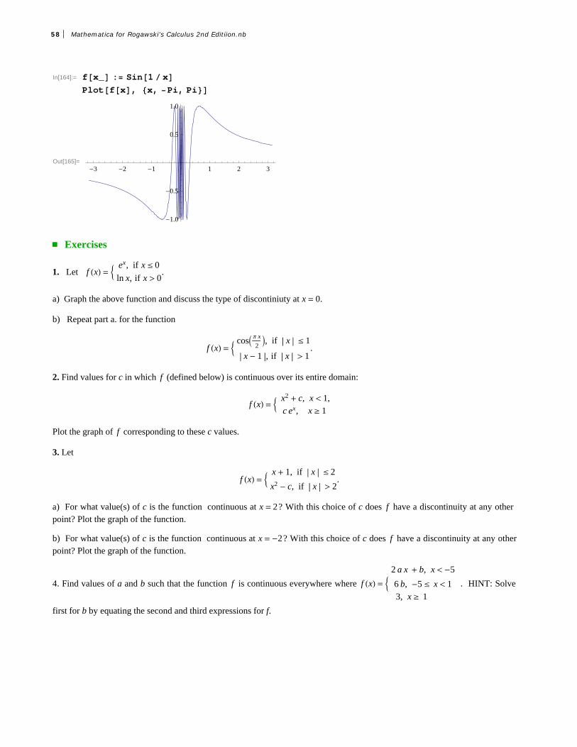
In[164]:= fx_ : Sin1 xPlotfx, x, Pi, Pi

Out[165]=-3 -2 -1 1 2 3

-1.0

-0.5

0.5

1.0

ü Exercises

1. Let f x = ex, if x § 0

ln x, if x > 0.

a) Graph the above function and discuss the type of discontiniuty at x = 0.

b) Repeat part a. for the function

f x = cos p x

2, if x § 1

x - 1 , if x > 1.

2. Find values for c in which f (defined below) is continuous over its entire domain:

f x = x2 + c, x < 1,

c ex, x ¥ 1

Plot the graph of f corresponding to these c values.

3. Let

f x = x + 1, if x § 2

x2 - c, if x > 2.

a) For what value(s) of c is the function continuous at x = 2? With this choice of c does f have a discontinuity at any otherpoint? Plot the graph of the function.

b) For what value(s) of c is the function continuous at x = -2? With this choice of c does f have a discontinuity at any otherpoint? Plot the graph of the function.

4. Find values of a and b such that the function f is continuous everywhere where f x = 2 a x + b, x < -5

6 b, -5 § x < 1

3, x ¥ 1

. HINT: Solve

first for b by equating the second and third expressions for f.


Chapter 3 Differentiation

ü 3.1 The Derivative

Students should read Sections 3.1-3.5 of Rogawski's Calculus [1] for a detailed discussion of the material presented in thissection.

ü 3.1.1 Slope of Tangent

The derivative is one of the most fundamental concepts in calculus. Its pointwise definition is given by

f £ a = limhØ0

f h + a - f ah

where geometrically f ' a is the slope of the line tangent to the graph of f x at x = a (provided the limit exists). We can viewthis graphically in the illustration below, where the tangent line (shown in blue) is viewed as a limit of secant lines (one shown inred) as hØ 0.

a a+h

Example 3.1. Calculate the derivative of f x = x2

3 at x = 1 using the pointwise definition of a derivative.

Solution: We first use the Table command to tabulate slopes of secant lines passing through the points at a = 1 and a + h = 1 + hby choosing arbitrarily small values for h (taken as reciprocal powers of 10):

In[166]:= fx_ x^2 3;a 1;h 10^n;TableFormNTableh, fa h fa

h, n, 1, 5


0.1 0.70.01 0.670.001 0.6670.0001 0.66670.00001 0.66667

Note our use of the TableForm command, which displays a list as an array of rectangular cells. From the table output, we infer

that f ' 1 = 2 3. A more rigorous approach is to algebraically simplify the difference quotient,f a+h- f a

h:


In[170]:= ClearhSimplify fa h fa

h

Out[171]=2 h

3

It is now clear that f a+h- f a

hØ 2

3as hØ 0. This can be checked using Mathematica's Limit command:

In[172]:= Limit fa h fah

, h 0

Out[172]=2

3

Below is a plot of the graph of f x (in black) and its corresponding tangent line (in blue), which also confirms our answer:

In[173]:= Plotfx, f'a x a fa, x, 2, 2, PlotStyle Black, Blue

Out[173]= -2 -1 1 2

-1.5

-1.0

-0.5

0.5

1.0

NOTE: Recall that the tangent line of f x at x = a is given by the equation y = f ' a x - a + f a.ANIMATION: Evaluate the following inputs to see animations of the secant lines approach the tangent line (from the right andleft).





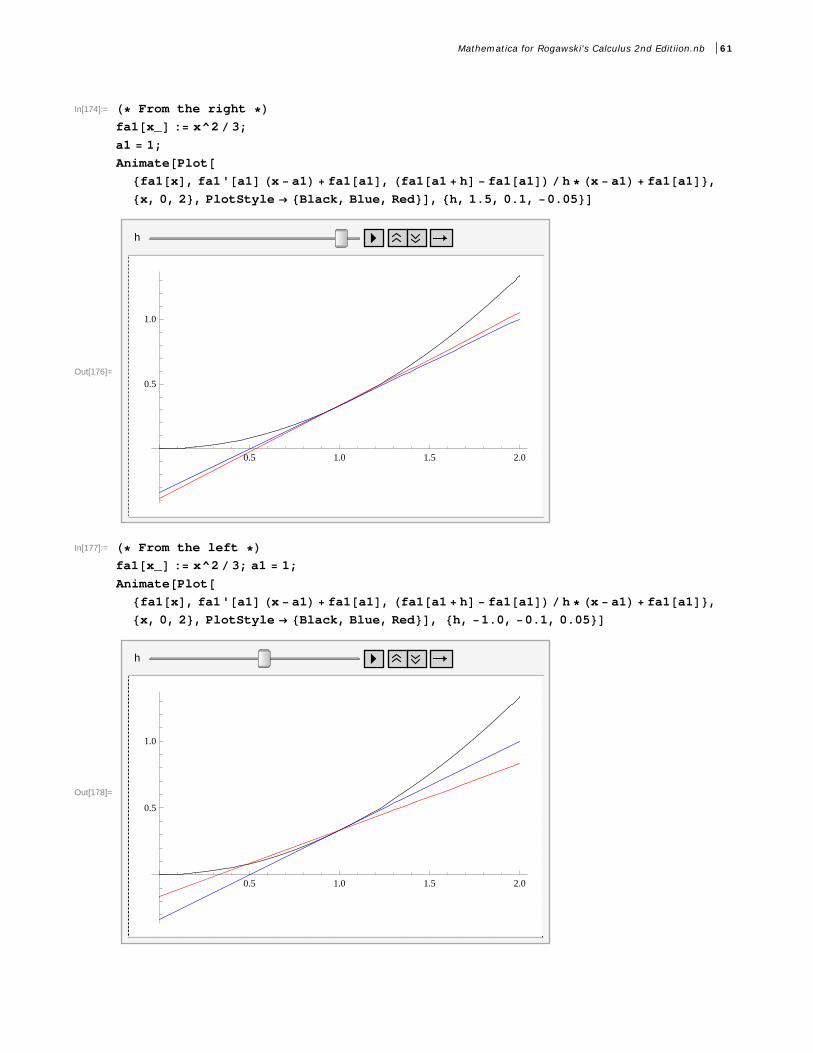
In[174]:= From the right fa1x_ : x^2 3;a1 1;AnimatePlot

fa1x, fa1'a1 x a1 fa1a1, fa1a1 h fa1a1 h x a1 fa1a1,x, 0, 2, PlotStyle Black, Blue, Red, h, 1.5, 0.1, 0.05

Out[176]=

h

0.5 1.0 1.5 2.0

0.5

1.0

In[177]:= From the left fa1x_ : x^2 3; a1 1;

AnimatePlotfa1x, fa1'a1 x a1 fa1a1, fa1a1 h fa1a1 h x a1 fa1a1,x, 0, 2, PlotStyle Black, Blue, Red, h, 1.0, 0.1, 0.05

Out[178]=

h

0.5 1.0 1.5 2.0

0.5

1.0


ü 3.1.2 Derivative as a Function

The derivative is best thought of as a slope function, one that gives the slope of the tangent line at any point on the graph of f xwhere this slope exists:

f £ x = limhØ0

f x + h - f xh

.

Example 3.2. Compute the derivative of f x = sin x using the limit definition.

Solution: We first simplify the corresponding difference quotient to obtain

In[179]:= Clearhfx_ Sinx;Simplifyfx h fx h

Out[181]=Sinx Sinh x

h

Here, it is not clear what the limit of the difference quotient is as hØ 0. To anticipate the answer for the derivative withoutalgebraic manipulation, we first note that since sin x is periodic, so should its derivative be. A plot of the difference quotient (as afunction of x) for several arbitrarily small values of h reveals the derivative to be cos x. Students should recognize from trigonom-etry that the graph of cos x is merely a left horizontal translation of sin x by

p

2.

In[182]:= plot1 Plotfx, Cosx, x, Pi, Pi, PlotStyle Black, Blue

Out[182]=-3 -2 -1 1 2 3

-1.0

-0.5

0.5

1.0

In[183]:= Clearhplot2 PlotEvaluateTablefx h fx h, h, 0.1, 0.7, 0.3,

x, Pi, Pi, PlotStyle Red

Out[184]=-3 -2 -1 1 2 3

-1.0

-0.5

0.5

1.0


In[185]:= Showplot1, plot2

Out[185]=-3 -2 -1 1 2 3

-1.0

-0.5

0.5

1.0

Of course, there are a number of methods to compute the derivative directly in Mathematica. One method is to evaluate the

command D f , x for a function f defined with respect to the variable x. A second method is to merely evaluate the expression

f'[x] using the traditional prime (apostrophe symbol) notation. A third method is to use the command ∑Ñ Ñ. We shall onlydiscuss the first two methods since the third method is usually reserved for derivatives of functions depending on more than onevariable, a topic that is treated in the third volume of this publication.

Example 3.3. Compute the derivative of sin x2 and evaluate it at x = p

4.

Solution:

Method 1:

In[186]:= DSinx^2, xDSinx^2, x . x SqrtPi 4

Out[186]= 2 x Cosx2

Out[187]=

2

NOTE: Recall the substitution command . x -> a was discussed in an earlier section.

Method 2:

In[188]:= fx_ Sinx^2f'xf'SqrtPi 4

Out[188]= Sinx2Out[189]= 2 x Cosx2

Out[190]=

2

Warning: Observe that the derivative of sin x2 is NOT cos x2 but 2 x cos x2. This is because sin x2 is a composite funct-

sion. A rule for differentiating composite functions, known as as the Chain Rule, is discussed in ection 3.7 of Rogawski'sCalculus.


Example 3.4. Compute the derivative of f x = sin x

xif x ∫ 0

0 if x = 0.

Solution: To define functions described by two different formulas over separate domains, we employ Mathematica's If[expr, p,

q] command:

In[191]:= fx_ Ifx 0, Sinx x, 0

Out[191]= Ifx 0,Sinx

x, 0

In[192]:= f'x

Out[192]= Ifx 0, Sinx

x2Cosx

x, 0

NOTE: It is clear for x ∫ 0 that the derivative is - sin x

x2+ cos x

x as a result of the Quotient Rule. For x = 0, Mathematica's answer

that f ' 0 = 0 is actually incorrect! Note that the fact that f 0 = 0 does not mean that f is a constant. One cannot differentiate aformula that is valid at only a single point; it is also necessary to understand how the function behaves in a neighborhood of thispoint.

A plot of the graph of f x reveals that it is discontinuous at x = 0, that is, limxØ0 f x ∫ f 0, and thus not differentiable there.

In[193]:= Plotfx, x, 3 Pi, 3 Pi

Out[193]=

-5 5

-0.2

0.2

0.4

0.6

0.8

1.0

Observe that the point f 0 = 0 is not distinguished in the Mathematica plot above so that the (removable) discontinuity isdetected only by examining the behavior of f around x = 0 (the true graph of f is shown following).


In particular, f xØ 1 as xØ 0. We confirm this with Mathematica.

In[194]:= Limitfx, x 0Out[194]= 1

Of course, it is also possible to compute f ' 0 directly from the limit definition. Here, the difference quotient behaves as sin h

h2 as

the output below shows. Since its limit does not exist as hØ 0, we conclude that f ' 0 is undefined.

In[195]:= Simplifyf0 h f0 hLimitf0 h f0 h, h 0

Out[195]=

Sinhh2

h 0

0 True

Out[196]=

NOTE: The discontinuity of f at x = 0 can be removed by redefining it there to be f 0 = 1. What is f ' 0 in this case?

Example 3.5 Find the equation of the tangent line to the graph of f(x) = x + 1 at x = 2.

Solution: Remember that the tangent line to a function f(x) at x = a is L(x) = f(a) + f '(a) (x-- a). Hear a = 2:

In[197]:=

Clearf, Lfx_ x 1

Lx_ f2 f'2 x 2Out[198]= 1 x

Out[199]= 3 2 x

2 3

To see that L(x) is indeed the desired tangent line, we will plot f and L together.


In[200]:= Plotfx, Lx, x, 0, 4

Out[200]=

1 2 3 4

1.2

1.4

1.6

1.8

2.0

2.2

Example 3.6. Find an equation of the line passing through the point P2, -3 and tangent to the graph of f x = x2 + 1.

Solution: Let us refer to Qa, f a as the point of tangency for our desired tangent line. To determine Q, we compute the slopeof our desired tangent line from two different perspectives:

1. Slope of line segment PQ:

In[201]:= Clearafx_ x^2 1

m fa 3 a 2Out[202]= 1 x2

Out[203]=4 a2

2 a

2. Derivative of f x at x = a:

In[204]:= fx_ x^2 1

f'aOut[204]= 1 x2

Out[205]= 2 a

Equating the two formulas for slope above and solving for a yields

In[206]:= Solvem f'a, aN

Out[206]= a 2 1 2 , a 2 1 2 Out[207]= a 0.828427, a 4.82843Since there are two valid solutions for a, we have in fact found two such tangent lines. Their equations are given by


In[208]:= Cleary1, y2y1x_ Simplifyf'a x a fa . a 2 1 2

y2x_ Simplifyf'a x a fa . a 2 1 2

Out[209]= 11 8 2 4 1 2 xOut[210]= 11 8 2 4 1 2 xPlotting these tangent lines together with the graph of f x confirms that our solution is correct:

In[211]:= Plotfx, y1x, y2x, x, 6, 6,PlotRange 10, 40, PlotStyle Black, Blue, Blue

Out[211]=

-6 -4 -2 2 4 6

-10

10

20

30

40

NOTE: How would the solution change if we move the given point in the problem to P2, 5? Or P2, 10?

ü Exercises

In Exercises 1 through 3, compute the derivatives of the given functions:

1. f x = 3 x2 + 1 2. gx = 1

x33. hx = sin x

cos x

In Exercises 4 and 5, evaluate the derivatives of the given functions at the specified values of x:

4. f x = x - 1 x + 1 at x = 1 5. gx = x +1

x -1 at x = 9

In Exercises 6 and 7, compute the derivatives of the given functions:6. f x = x + 3 7. gx = x2 - 4

Hint: Recall the absolute value function: x = x if x ¥ 0

-x if x < 0. Use the If command to define these absolute functions (see

Example 3.4). Note that Mathematica does have a built-in Absx command for defining the absolute value of x, but Mathemat-ica treats Absx as a complex function; thus its derivative Abs 'x is NOT defined. The real derivative of Absx for real values

of x can still be found using the numerical derivative ND command but we shall not discuss it here.

8. Find an equation of the line tangent to the graph of x - y2 = 0 at the point P9, -3.9. Find an equation of the line passing through the point P2, -3 and tangent to the graph of y = x2.

ü 3.2. Higher-Order Derivatives



Suppose one is interested in securing higher order derivatives of a function. Reasons for doing so include applications to maxi-mum and minimum values, points of inflection, and physical applications such as velocity and acceleration and jerk, which all fitinto such a context.

Example 3.6. Compute the first eight derivatives of f x = sin x. What is the 255th derivative of f ?

Solution: Here are the first eight derivative of f :

In[212]:= fx_ Sinx;TableFormTablen, Dfx, x, n, n, 1, 8


1 Cosx2 Sinx3 Cosx4 Sinx5 Cosx6 Sinx7 Cosx8 Sinx

We observe from the output that the higher-order derivatives of f are periodic modulo 4, which means they repeat every fourderivatives. Since 255 has remainder 3 when divided by 4, it follows that f 255x = f 3x = -cos x. Of course, Mathematicacan compute this derivative directly (see output below), but the pattern above gives us a more in-depth understanding of thehigher-order derivatives of sin x.

In[214]:= Dfx, x, 255Out[214]= CosxExample 3.7. Compute the first three derivatives of f x = x cos x .

Solution: We use the command D f , x, n to compute the nth derivative of f. Here, we set n = 1, 2, 3.

In[215]:= fx_ x CosxOut[215]= x CosxIn[216]:= Dfx, xOut[216]= Cosx x SinxIn[217]:= Dfx, x, 2Out[217]= x Cosx 2 SinxIn[218]:= Dfx, x, 3Out[218]= 3 Cosx x SinxA quicker way to generate a list of higher-order derivatives is to use the Table command. For example, here is a list of the firstfive derivatives of f :


In[219]:= TableDfx, x, n, n, 1, 5Out[219]= Cosx x Sinx, x Cosx 2 Sinx,

3 Cosx x Sinx, x Cosx 4 Sinx, 5 Cosx x SinxDiscovery Exercise: Find a formula for the nth derivative of f based on the pattern above. Can you prove your claim usingmathematical induction? What is the 100th derivative of f in this case? Check your answer using Mathematica.

ü Exercises

1. Let f x = 1 x.a) Compute the first five higher-order derivatives of f .b) What is the 10th derivative of f ?c) Obtain a general formula for the nth derivative based on the pattern. Then use the principle of mathematical induction tojustify your claim.

2. Consider f x = x sin x. Determine the first eight derivatives of f and obtain a pattern. Justify your contention.

In Exercises 3 and 4, compute f k(x) for k = 1,2,3,4.

3. f x = 1 + x26

5

4 . f x = 1-x2

1-3 x+2 x3

ü 3.3 Chain Rule and Implicit Differentiation

Students should read Sections 3.7 and 3.10 of Rogawski's Calculus [1] for a detailed discussion of the material presentedin this section.

In this section, we demonstrate not only how Mathematica uses the Chain Rule to differentiate composite functions but also tocompute derivatives of functions defined implicitly by equations where solving for the dependent variable is not feasible.

Example 3.8. Find all horizontal tangents of f x = x4-x+1

x4+x+1 .

Solution: We first compute the derivative of f , which requires the Chain Rule.

In[220]:= fx_ :x4 x 1

x4 x 1;

Simplifyf'x

Out[221]=1 3 x4

1xx4

1xx41 x x42

Horizontal tangents have zero slope and so it suffices to solve f ' x = 0 for x.

In[222]:= Solvef'x 0, x

Out[222]= x 1

314, x

314, x

314, x

1

314


Observe that the solutions above are nothing more than the zeros of the numerator of f ' x. We ignore the second and third

solutions listed above, which are imaginary. Hence, x = 1 34

º 0.76 and x = - 1 34

. A plot of the graph of f belowconfirms our solution.

In[223]:= Plotfx, x, 2, 2

Out[223]=

-2 -1 1 2

0.8

1.0

1.2

1.4

1.6

1.8

Example 3.9. Find all horizontal tangents of the lemniscate described by 2 x2 + y22 = 25 x2 - y2.

Solution: Implicit differentiation is required here to compute d y

d x, which involves first differentiating the lemniscate equation and

then solving for our derivative. Observe that we make the substitution yØ yx, which makes explicit our assumption that ydepends on x.

In[224]:= Clearx, yeq 2 x^2 y^2^2 25 x^2 y^2

Out[225]= 2 x2 y22 25 x2 y2

In[226]:= 2 x2 y22 25 x2 y2Out[226]= 2 x2 y22 25 x2 y2In[227]:= deq Deq . y yx, xOut[227]= 4 x2 yx2 2 x 2 yx yx 25 2 x 2 yx yxIn[228]:= Solvedeq, y'x

Out[228]= yx 25 x 4 x3 4 x yx2

yx 25 4 x2 4 yx2

To find horizontal tangents, it suffices to find where the numerator of y ' x vanishes (since the denominator never vanishes

except when y = 0). Thus, we solve the system of equations 25 x - 4 x3 - 4 x y2 = 0 and 2 x2 + y22 = 25 x2 - y2 since the

solutions must also lie on the lemniscate.

In[229]:= Solveeq, 25 x 4 x^3 4 x y^2 0, x, y

Out[229]= x 0, y 0, x 0, y 5

2, x 0, y

5

2, x

5 3

4, y

5

4,

x 5 3

4, y

5

4, x

5 3

4, y

5

4, x

5 3

4, y

5

4


From the output, we see that there are four valid solutions at 5 3 4, 5 4 º 2.17, 1.25, -5 3 4, 5 4,5 3 4, -5 4, and -5 3 4, -5 4, which can be confirmed by inspecting the graph of the lemniscate below. Observe

the symmetry in the solutions.

In[230]:= N5 Sqrt3 4Out[230]= 2.16506

In[231]:= ContourPlot2 x^2 y^2^2 25 x^2 y^2, x, 4, 4, y, 2, 2

Out[231]=

-4 -2 0 2 4-2

-1

0

1

2

ü Exercises

1. Find all horizontal tangents of gx = x2

x+17

.

2. Find all tangents along the curve hx = x + x whose slope equals 1/2.

3. Find all vertical tangents of the cardioid described by x2 + y2 = 2 x2 + 2 y2 - x2.

4. Compute the first and second derivatives of

f x = x cos1

xif x ∫ 0

0 if x = 0.

5. Compute the first and second derivatives of

gx = x2 cos1

xif x ∫ 0

0 if x = 0.

How do these derivatives at the origin compare with those in the previous exercise?

6. Based on your investigations of the previous two exercises, explain the behavior of higher-order derivatives of

hx = xn cos1

xif x ∫ 0

0 if x = 0

at the origin for positive integer values of n.

7. Calculate the implicit derivative of y with respect to x of: xy2 + x2 y4-- x3 = 5.


8. Plot x2 + y22 = x2 - y2+2 for -4 § x § 4 and -4 § y § 4. Then determine how many horizontal tangent lines the

curve appears to have and find the points where these occur.

ü 3.4 Derivatives of Inverse, Exponential, and Logarithmic Functions


Exponential functions arise naturally. For example, mathematical models for the growth of a population or the decay of a radioac-tive substance involve exponential functions. In this section, we will explore exponential functions and their inverses, calledlogarithmic functions, using Mathematica. We begin with a review of inverse functions in general.

ü 3.4.1. Inverse of a Function

Recall that a function gx is the inverse of a given function f x if f gx = g f x = x. The inverse of f x is denoted by f -1x. We note that a necessary and sufficient condition for a function to have an inverse is that it must be one-to-one. On the other hand, a function is one-to-one if it is strictly increasing or strictly decreasing throughout its domain.

Example 3.13. Determine if the function f x = x2 - x + 1 has an inverse on the domain -¶, ¶. If it exists, then find theinverse.

Solution: We note that f 0 = f 1 = 1. Thus, f is not one-to-one. We can also plot the graph of f and note that it fails theHorizontal Line Test since it is not increasing on its domain.

In[232]:= Clearf, gIn[233]:= fx_ x^2 x 1;

Plotfx, x, 1, 2

Out[234]=

-1.0 -0.5 0.5 1.0 1.5 2.0

1.5

2.0

2.5

3.0

However, observe that if we restrict the domain of f to an interval where f is either increasing or decreasing, say 0.5, ¶, thenits inverse exists (see plot below).


In[235]:= plotf Plotfx, x, 0.5, 5

Out[235]=

2 3 4 5

5

10

15

20

To find the inverse on this restricted domain, we set y = f -1x. Then f y = x. Thus, we solve for y from the equation f y = x.

In[236]:= sol Solvefy x, y

Out[236]= y 1

21 3 4 x , y

1

21 3 4 x

Note that Mathematica gives two solutions. Only the second one is valid, having range 0.5, ¶, which agrees with the domain off . Thus,

f -1x = 1

21 + -3 + 4 x .

To extract this solution from the above output, we use the syntax below and denote the inverse function in Mathematica by gx(Mathematica interprets the notation f -1x as 1

f x , the reciprocal of f ).

In[237]:= gx_ sol2, 1, 2

Out[237]=1

21 3 4 x

To verify that f gx = x, we use the Simplify command.

In[238]:= Simplifyfgx xOut[238]= True

NOTE: One can also attempt to verify g f x = x. However, Mathematica cannot confirm this identity (see output below)because it is unable to simplify the radical, which it treats as a complex square root. Students are encouraged to algebraicallycheck this identity on their own.

In[239]:= Simplifygfx x

Out[239]= 1 1 2 x2 2 x

Lastly, a plot of the graphs of f x and gx (in black and blue, respectively) shows their expected symmetry about the diagonalline y = x (in red). Observe that the domain of g is 3 4, ¶, which is the range of f .


In[240]:= plotg Plotgx, x, 3 4, 5, PlotStyle Red, AspectRatio Automatic

Out[240]=

2 3 4 5

1.0

1.5

2.0

2.5

In[241]:= Showplotf, plotg, GraphicsDashing0.05, 0.05, Line0, 0, 5, 5,PlotRange 0, 5, AspectRatio Automatic

Out[241]=

0 2 3 4 5

1

2

3

4

5

Example 3.14. Determine if the function f x = x3 + x has an inverse. If it exists, then compute f -1 ' 2.Solution: Since f ' x = 3 x2 + 1 > 0 for all x, we see that f is increasing on its domain. Thus, it has an inverse. Again, we cansolve for this inverse as in the previous example:


In[242]:= Clearf, g, x, solfx_ : x^3 x

sol Solvefy x, y

Out[244]= y 2313

9 x 3 4 27 x213

9 x 3 4 27 x213

213 323,

y 1 3

223 313 9 x 3 4 27 x213

1 3 9 x 3 4 27 x213

2 213 323,

y 1 3

223 313 9 x 3 4 27 x213

1 3 9 x 3 4 27 x213

2 213 323

Only the first solution listed above is valid, being real valued. Thus,

f -1x = - 2

313

9 x+ 3 4+27 x213 +

9 x+ 3 4+27 x213

213 323 .

Again we denote our inverse by gx:In[245]:= gx_ sol1, 1, 2

Out[245]= 2313

9 x 3 4 27 x213

9 x 3 4 27 x213

213 323

Lastly, we compute g ' 2. In[246]:= Simplifyg'2

NOut[246]= 313 14 3 21 313 9 2 21 23 28 9 2 21 43Out[247]= 0.25

NOTE: The easier approach in computing g ' 2 without having to explicitly differentiate gx is to instead use the relation f -1 ' x = 1 f ' f -1x, which shows that the derivative of f at a point a, b on its graph and the derivative of f -1 (or g in our

case) at the corresponding inverse point b, a on its graph are reciprocal. In particular, since f 1 = 2 and f -12 = 1, we have f -1 ' 2 = 1 f ' f -12 = 1 f ' 1 = 1 4.


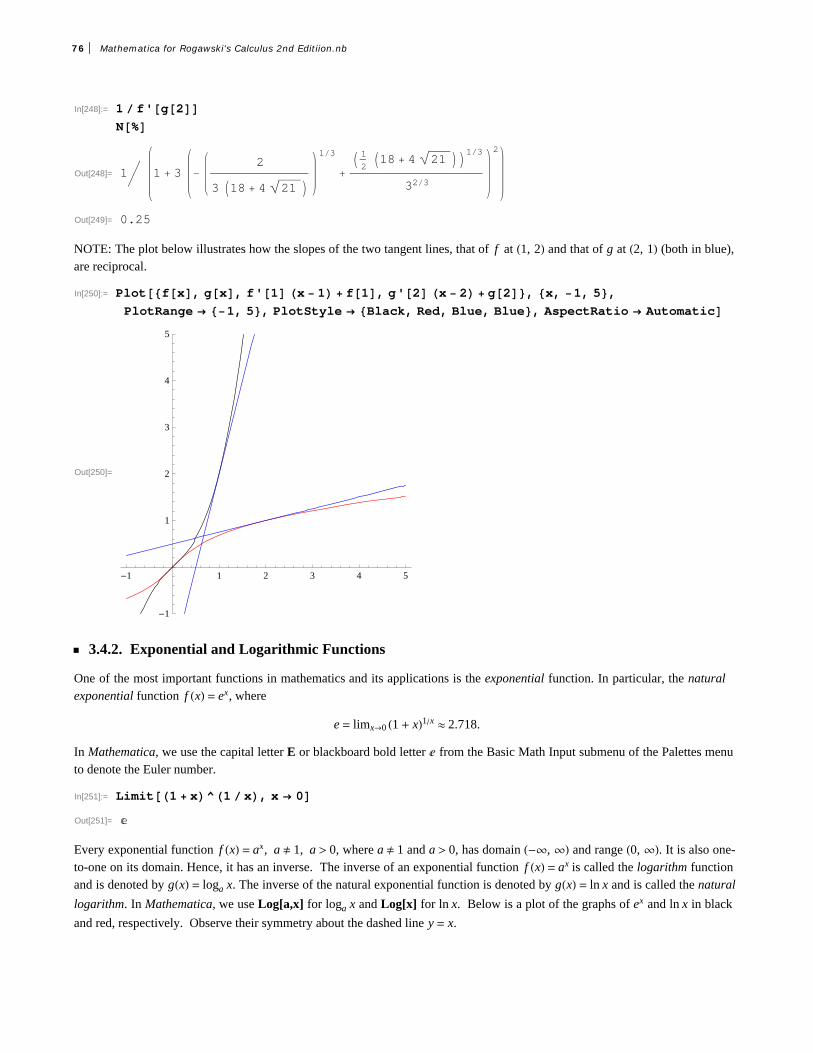
In[248]:= 1 f'g2N

Out[248]= 1 1 3 2

3 18 4 21

13 1218 4 21 13

323

2

Out[249]= 0.25

NOTE: The plot below illustrates how the slopes of the two tangent lines, that of f at 1, 2 and that of g at 2, 1 (both in blue),are reciprocal.

In[250]:= Plotfx, gx, f'1 x 1 f1, g'2 x 2 g2, x, 1, 5,PlotRange 1, 5, PlotStyle Black, Red, Blue, Blue, AspectRatio Automatic

Out[250]=

-1 1 2 3 4 5

-1

1

2

3

4

5

ü 3.4.2. Exponential and Logarithmic Functions

One of the most important functions in mathematics and its applications is the exponential function. In particular, the naturalexponential function f x = ex, where

e = limxØ0 1 + x1x º 2.718.

In Mathematica, we use the capital letter E or blackboard bold letter ‰ from the Basic Math Input submenu of the Palettes menuto denote the Euler number.

In[251]:= Limit1 x^1 x, x 0Out[251]=

Every exponential function f x = ax, a ∫ 1, a > 0, where a ∫ 1 and a > 0, has domain -¶, ¶ and range 0, ¶. It is also one-to-one on its domain. Hence, it has an inverse. The inverse of an exponential function f x = ax is called the logarithm functionand is denoted by gx = loga x. The inverse of the natural exponential function is denoted by gx = ln x and is called the natural

logarithm. In Mathematica, we use Log[a,x] for loga x and Log[x] for ln x. Below is a plot of the graphs of ex and ln x in black

and red, respectively. Observe their symmetry about the dashed line y = x.


-2 -1 1 2 3 4 5

-2

-1

1

2

3

4

5

Please refer to Section 3.9 of Rogawski's Calculus textbook for derivative formulas of general exponential and logarithmicfunctions.

Example 3.15. Compute derivatives of the following functions.a) f x = 2x b) f x = 6 x2 + 4 ex c) f x = log10 x2 d) f x = lncose3 xSolution: We will input the functions directly and use the command D to find each derivative. Thus, for a) we will evaluateD2x, x. Again, note that Log[2] should be read as ln 2.

a)

In[252]:= D2^x, xOut[252]= 2x Log2b)

In[253]:= D6 x2 4 Ex, xOut[253]= 4 x 12 x

c)

In[254]:= DLog10, x^2, x

Out[254]=2

x Log10d)

In[255]:= f DLogCosE3 x, xOut[255]= 3 3 x Tan3 xExample 3.16. Find points on the graph of f x = x2 e3 x+5 + 3 x where the tangent lines are parallel to the line y = 3 x - 1.

Solution: Since the slope of the given line equals 3 it suffices to solve f ' x = 3 for x to locate these point(s).


In[256]:= Clearf, solfx_ x2 E3 x5 3 x

sol Solvef'x 3, xOut[257]= 3 x 53 x x2

Out[258]= x 2

3, x 0

Thus there are two solutions: -2 3, -2 + 4 e3 9 and 0, 0.In[259]:= x0 sol1, 1, 2

x1 sol2, 1, 2fx0fx1

Out[259]= 2

3

Out[260]= 0

Out[261]= 2 4 3

9

Out[262]= 0

The plot that follows on the next page confirms that the two corresponding tangent lines (in blue) are indeed parallel to the givenline (in red).

In[263]:= y1 fx0 f'x0 x x0y2 fx1 f'x1 x x1Plotfx, y1, y2, 3 x 2, x, 1, 1,PlotRange 5, 15, PlotStyle Black, Blue, Blue, Red

Out[263]= 2 4 3

9 3

2

3 x

Out[264]= 3 x

Out[265]=

-1.0 -0.5 0.5 1.0

-5

5

10

15


NOTE: One would expect the tangent line at the origin to be horizontal based on a visual inspection of the graph of f , but thisdemonstrates the pitfall of using a graphing approach.

ü Exercises

In Exercises 1 through 4, compute derivatives of the given functions.

1. f x = x2 ex3-4 x 2. f x = xa + ax

3. f x = ln x - 1 + lnx + 14. f x = log10x x3-3 x+1

x2-2 x-332

5. Find the second and third derivatives of f x = ex ln x.

6. Let f x = cos x + ln x. Plot the graphs of f and f ' on the same set of axes.

7. Find an equation of the line tangent to the graph of f x = ln x

x2 that is parallel to the x-axis.

8. Discovery Exercise: Define sinh x = ex - e-x 2 and cosh x = ex + e-x 2. These functions are called the hyperbolic sine andhyperbolic cosine of x, respectively.

a) Determine the initial eight derivatives of each of these two hyperbolic functions.

b) Determine general formulas for the nth derivatives of these functions based on the pattern and verify your contentions viamathematical induction.

c) How do the higher-order derivatives of sinh x and cosh x compare with those of the trigonometric functions sin x and cos x?


Chapter 4 Applications of the DerivativeWe have seen how the derivative of a function is itself a function. This idea leads to many possible applications, some of whichwe will now explore with Mathematica to demonstrate its ability to manipulate and calculate complicated or tedious expressions.

ü 4.1 Related Rates


Example 4.1. Let us assume a rubber ball is sitting out in the sun and that the heat causes its surface area to increase at the rateof 1.5 square centimeters per hour. How fast is the radius increasing when the radius is 2 centimeters?

Solution: To solve this problem, we will need the formula for the surface area of a sphere: S = 4pr2. Here, the surface area S andthe radius r are expressed as functions of t (time).

In[266]:= ClearSsa St 4 rt^2

Out[267]= St 4 rt2In[268]:= dsa Dsa, tOut[268]= St 8 rt rtNow differentiate this formula and solve for r ' t:In[269]:= sol Solvedsa, r't

Out[269]= rt St

8 rt

Since the output above is a nested list (each set of curly braces denotes a list; see Chapter 1 of this manual for a description of

nested lists) and our solution, S' t8 p rt , represents the second element of the first (inner) list, we can extract it in order to define r ' t

as follows:

In[270]:= r't sol1, 1, 2

Out[270]=St

8 rtSince we are given that S ' t = 1.5 and rt = 2, we substitute these into the formula for r ' t:In[271]:= r't . S't 1.5, rt 2Out[271]= 0.0298416

Therefore, when the radius is 2 cm, it is increasing at the rate of about .0298 cm per hour.

ü Exercises

1. If the volume of a cube is increasing at the rate of 2 cubic inches per minute, how fast is the length of one of its sides increas-ing when that side is 8 inches?


2. A particle is moving along a parabola y = 2 x2 + 3 x - 1 in such a way that the rate of change of its x-coordinate is constant,namely x ' t = 3. Find the rate of change of its y-coordinate when the position of the particle is (1,4).

3. The radius r and height h of a circular cone change at a rate of 2 cm/s. How fast is the volume of the cone increasing when r =10 and h = 20? (Recall that the volume of a cone is pr2h/3.)

ü 4.2 Extrema


Next, let us consider finding critical points and inflection points to determine extrema. Remember that critical points of afunction are those for which f ' x = 0 or for which f ' x does not exist. Similarly, inflection points occur where eitherf '' x = 0 or where f '' x does not exist. Extrema occur at critical points, but not all critical points are extrema (consult yourcalculus text). An inflection point is a point c, f c where concavity changes; this occurs where f '' c = 0 or wheref '' x does not exist, and like critical points, not all points where f '' x = 0 (or where f '' x does not exist) are inflection points.

Example 4.2. Find all local extrema and inflection points of f x = 1x2 + 3.Solution: We first define f in Mathematica:

In[272]:= Clear f, xIn[273]:= fx_ : 1 x^2 3In[274]:= Plot fx, x, 4, 4

Out[274]=

-4 -2 2 4

0.10

0.15

0.20

0.25

0.30

To find extrema of f , we locate its critical points, that is, those points where f ' x = 0 or f ' x is undefined. We can solve thefirst case using Mathematica:

In[275]:= f'xSolvef'x 0, x

Out[275]= 2 x

3 x22

Out[276]= x 0Since f ' x is defined everywhere, it follows that there is exactly one critical point at x = 0, and at that point, there is a maxi-mum, as can be seen from the graph above. We could also have used the second derivative test to confirm this:


In[277]:= f''0

Out[277]= 2

9

Since the second derivative is negative at x = 0, the curve is concave down there. This, of course, means that we have a localmaximum at x = 0.

To find the points of inflection, we locate zeros of the second derivative:

In[278]:= Solvef''x 0, xOut[278]= x 1, x 1To determine if these solutions are indeed inflection points, we need to check if there is a sign change in f '' x on either side ofeach (at x = -1 and x = 1):

In[279]:= Plotf''x, x, 2, 2

Out[279]=

-2 -1 1 2

-0.20

-0.15

-0.10

-0.05

0.05

Notice from the graph above that f '' x changes from positive to negative at x = -1 and from negative to positive at x = 1. Thusboth points -1, f -1 and 1, f 1 are inflection points.

ü Exercises

In Exercises 1through 5, find all critical points and inflection points for:1. f x = x3 - 3 x2 + 1 2. f x = x2 - 3 ‰x 3. f x = sin x on [0, 2p]

4. f x = 2 x5 - 5 x4 + 5 5. f x = x2+4

x

6. Consider the function f x = xn where n is a positive integer. For what values of n do we have a) a relative minimum but not a point of inflection at the origin?b) a point of inflection at the origin but not a relative minimum?Sketch the graph of several power functions to support your reasoning.

ü 4.3 Optimization


Extreme values of a function occur where f ' x = 0 or where f ' x does not exist. This idea allows us to find maxima andminima, concepts that are crucial in many applications. For instance, in business, one wants to minimize costs or maximizeprofits. In government, one wants to track the flow of money in an economy, and when that flow is a minimum or a maximum.


In engineering design, we may want to know what shape of a conduit will generate maximum flow. Similar problems exist inmany other fields. We will now look at some of these applications.

ü 4.3.1 Traffic Flow

Example 4.3. Traffic flow along a major highway in Boston between 6 AM and 10 AM can be modeled by the function

f t = 20 t - 40 t + 50 (in miles per hour), where t = 0 corresponds to 6 AM. Determine when the minimum traffic flowoccurs.

Solution: Let us first plot the graph of f t.In[280]:= Clearf, tIn[281]:= ft_ : 20 t 40 t 50

In[282]:= Plotft, t, 0, 4

Out[282]=

1 2 3 4

35

40

45

50

Note from the plot above that the average speed is decreasing between 6 AM and 7 AM and increasing after 7 AM.

At 6 AM the average speed is

In[283]:= f0Out[283]= 50

or 50 mph. At 6:30 AM the average speed is

In[284]:= f.5Out[284]= 31.7157

or 31.7 mph. To see how the average speed varies throughout the day we make a table of these values at each half hour from 6AM to 10 AM:


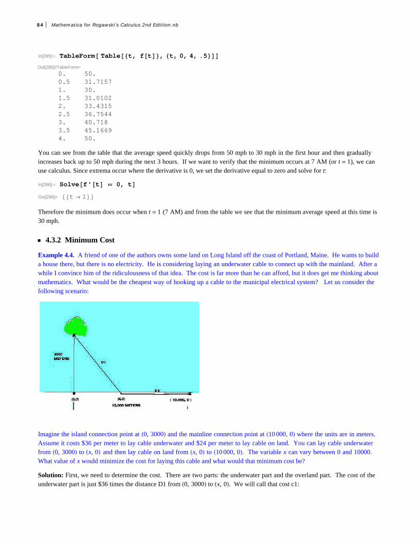
In[285]:= TableForm Tablet, ft, t, 0, 4, .5Out[285]//TableForm=

0. 50.0.5 31.71571. 30.1.5 31.01022. 33.43152.5 36.75443. 40.7183.5 45.16694. 50.

You can see from the table that the average speed quickly drops from 50 mph to 30 mph in the first hour and then graduallyincreases back up to 50 mph during the next 3 hours. If we want to verify that the minimum occurs at 7 AM (or t = 1), we canuse calculus. Since extrema occur where the derivative is 0, we set the derivative equal to zero and solve for t:

In[286]:= Solvef't 0, tOut[286]= t 1Therefore the minimum does occur when t = 1 (7 AM) and from the table we see that the minimum average speed at this time is30 mph.

ü 4.3.2 Minimum Cost

Example 4.4. A friend of one of the authors owns some land on Long Island off the coast of Portland, Maine. He wants to builda house there, but there is no electricity. He is considering laying an underwater cable to connect up with the mainland. After awhile I convince him of the ridiculousness of that idea. The cost is far more than he can afford, but it does get me thinking aboutmathematics. What would be the cheapest way of hooking up a cable to the municipal electrical system? Let us consider thefollowing scenario:

Imagine the island connection point at 0, 3000 and the mainline connection point at 10 000, 0 where the units are in meters.Assume it costs $36 per meter to lay cable underwater and $24 per meter to lay cable on land. You can lay cable underwaterfrom 0, 3000 to x, 0 and then lay cable on land from x, 0 to 10 000, 0. The variable x can vary between 0 and 10000.What value of x would minimize the cost for laying this cable and what would that minimum cost be?

Solution: First, we need to determine the cost. There are two parts: the underwater part and the overland part. The cost of theunderwater part is just $36 times the distance D1 from 0, 3000 to x, 0. We will call that cost c1:


In[287]:= c1x_ : 36 30002 x2

The overland cost is $24 times the distance D2 from x, 0 to 10 000, 0. We will call that cost c2:

In[288]:= c2x_ : 24 10000 xThe total cost is then

In[289]:= costx_ c1x c2x

Out[289]= 24 10000 x 36 9000000 x2

We need to minimize this cost function. First, we graph it to see if it has a minimum:

In[290]:= Plotcostx, x, 0, 10000

Out[290]=

2000 4000 6000 8000 10 000

330 000

340 000

350 000

360 000

370 000

Notice that this cost function has its minimum somewhere between 2000 and 4000. Also, you will note that as x gets close to thatminimum the tangent lines of cost x) are getting close to horizontal. In other words, the minimum will occur at a point x forwhich the derivative is zero or horizontal (i.e., the derivative at a point gives the slope of the tangent line at that point). This is acalculus problem that we can solve.

In[291]:= Solvecost'x 0, xOut[291]= x 1200 5

In[292]:= Ncost1200 5 Out[292]= 320498.

Therefore, the minimum occurs at x = 1200 5 º 2683.28 meters and the minimum cost is approximately $320,498.

NOTE: Another method in finding the minimum is to use the command FindMinimum. We will start our search near x = 2000:

In[293]:= FindMinimumcostx, x, 2000, WorkingPrecision 8Out[293]= 320498.45, x 2683.2816Again, we get an answer that corroborates the previous answer.

ü 4.3.3 Packaging (Minimum Surface Area)

Example 4.5. A major concern in business is to minimize the cost of packaging. This cost is related to the surface area of thepackage. If we can minimize that surface area, then we can minimize the cost. Let us assume that a company has a certain


product that needs to be packaged in a rectangular box having a square base. If the volume of the box is required to be 1 cubicmeter, then find the dimensions of the box that will minimize its surface area.

Solution: If the length of the sides of the square base is x and the height of the box is y, then the volume of the box is given byx2 y and must equal 1 cubic meter (this is our constraint):

In[294]:= Clearx, y, SIn[295]:= constraint x^2 y 1

Out[295]= x2 y 1

The surface area of our package (box) is S = 4 x y + 2 x2 and is the quantity that must be minimized (recall that the top and

bottom sides each have area x2 and the 4 sides each have area x y). Using our volume constraint, x2y = 1, we can solve for y interms of x:

y = 1

x2

In[296]:= sol Solveconstraint, y

Out[296]= y 1

x2

The surface area function can then be expressed as a function of x only:

S x = 4 x y + 2 x2 = 4 x 1x2 + 2 x2 = 4 x + 2 x2

In[297]:= Sx_ 4 x y 2 x^2 . y sol1, 1, 2

Out[297]=4

x 2 x2

Using the idea again that extrema occur at points where the derivative is zero, we calculate:

In[298]:= SolveS'x 0, xOut[298]= x 1, x 113, x 123This equation has 1 real and 2 imaginary solutions. We need only the real solution of x = 1. To see that this corresponds to anactual minimum, we plot the curve:


In[299]:= PlotSx, x, 0 , 5

Out[299]=

1 2 3 4 5

20

30

40

50

60

70

80

Alternatively, we could have used the second derivative test to show that a minimum occurs at x = 1:

In[300]:= S''1Out[300]= 12

Since f '' 1 > 0, we know that the graph is concave up at x = 1 and hence must have a minimum there. Since y = 1 when x = 1,we conclude that the box with minimum surface area is a cube with sides of 1 meter.

ü 4.3.4 Maximize Revenue

The following application concerns optimizing group fares for charter flights.

Example 4.6. Suppose a travel agency charges $600 per person for a charter flight if exactly 100 people sign up. However, ifmore than 100 people sign up, then the fare is reduced by $2 per person for each additional person over the initial 100. The travelagency wants to know how many people they should book to maximize revenue. Also, determine what that maximum revenue isand what the corresponding fare is for each person.

We let x denote the number of passengers above 100. Keep in mind that revenue is the product of the number of people multi-plied by the cost (fare) per person. If R x is defined as the revenue function, then R x = 100 + x 600 - 2 x. To determinethe maximum value of R x for x ¥ 0, let us first examine its graph:

In[301]:= Rx_ : 100 x 600 2 x


In[302]:= PlotRx, x, 0, 200

Out[302]=

50 100 150 200

65 000

70 000

75 000

80 000

From the plot above, we see that a maximum occurs at about x = 100. To confirm this, we first solve for the critical points:

In[303]:= SolveR'x 0, xOut[303]= x 100Therefore the maximum does indeed occur at x = 100, and the maximum revenue is

In[304]:= R100Out[304]= 80000

or $80,000. Since 100 + x represents the number of customers, this occurs when 200 customers sign up for the flight. In thiscase, the cost per person is

In[305]:= 600 2 x . x 100

Out[305]= 400

or $400 per person.

ü Exercises

1. Assume traffic flow is given by a speed function f t = 25 t - 45 t + 55. Analyze speed changes between 6 AM and 10AM and calculate when traffic flow is minimized. What is that minimum speed?

2. Find the minimum value of f x = 3 x4 + 4 x3.

3. Assume that the average cost of producing compact discs is given by c x = -.0002 x + 3 + 2000 x. Show that the averagecost is always decreasing for x between 0 and 4000.

4. Suppose the population of a city is modeled by

p t = 4456 t3 + 8939 t2 + 23 463 t + 25 528

where t is measured in years from 1990 to 2000.

a) Show that the population was always increasing in this decade.


b) Show that the population was increasing at its slowest rate in August of 1990. Hint: The population is increasing at itsslowest rate when p '' t = 0.

5. Given that the total cost for manufacturing x units of a particular product is described by the functionCx = 0.0025 x2 + 80 x + 10 000, find the level of production that minimizes the total cost of manufacturing.

6. The total population of the planet is forecast by the function Pt = 0.00074 t3 - 0.07 t2 + 0.89 t + 6.04 where t is measured indecades, t = 0 corresponds to the year 2000, and Pt is measured in billions of people. In what year will the population peakover the next 200 years?

7. A book designer has decided that the pages of a book are to have 1.5 inch margins top and bottom and 1 inch margins on eachside. If each page is to have an area of 100 square inches, what are the dimensions of this page if its printed area is to be amaximum?

8. The owner of a farm wants to enclose a rectangular region with 3000 m of fencing while dividing the region into two parts,each of which is rectangular, by using part of the fencing to subdivide it and running a fence parallel to the sides (see figure thatfollows). What should be the dimensions of the region in order to maximize its area?

9. The owner of a cruise ship charges groups as follows: For a group of 40 people, the charge is $1,000 per person per day. Ifmore than 40 people sign up, the fare is reduced by $8 for each addtional person.

a) Assuming at least 40 people sign up, determine the number necessary to maximize revenue.

b) What is the maximum revenue?

c) What would be the cost per person in this case?

ü 4.4 Newton's Method


ü 4.4.1 Programming Newton's Method

Newton's Method is a technique for calculating zeros of a function based on the direction of its tangent lines. It is a recursiveroutine that is rather tedious to do by hand or even with a calculator, but simple with Mathematica. To start the procedure oneshould have an idea about the general location of each zero. This is because an initial approximation x0 for that zero, say at x = r,is needed to start the recursion. For example, one can specify x0 by examining the graph of the function to see where the zerosare approximately. Then the next approximation x1 can be found by the recursive formula x1 = x0 - f x0 f ' x0. This processcan be iterated using the general formula


xn+1 = xn - f xn f ' xnUnder suitable conditions, the sequence of approximations x0, x1, x2, ... (called the Newton sequence) will converge to r.

Example 4.7. Approximate the zeros of the function f x = ln9 - x2 - x.

In[306]:= fx_ : Log9 x2 xIn[307]:= Plotfx, x, 0, 3

Out[307]=

0.5 1.0 1.5 2.0 2.5 3.0

-4

-2

2

Clearly, there is one zero between 1.5 and 2 based on the plot above. To approximate this zero, we define a function newtn toperform the recursion:

In[308]:= newtnx_ : x fx f'xTo generate the corresponding Newton sequence, we compute 8 iterates of this function starting with an initial guess of x = 1.6.

This iteration can be performed efficiently using the NestList[f,x,n] function, which is a recursive routine that outputs a list with

x as its first value, followed by f[x], f[f[x]], f[f[f[x]]], etc., up to n iterates as shown in the example below:

In[309]:= approx NestListnewtn, 1.6, 8Out[309]= 1.6, 1.77538, 1.76961, 1.7696, 1.7696, 1.7696, 1.7696, 1.7696, 1.7696From this we see that the root, accurate to 4 decimal places, is 1.7696. If greater accuracy is desired, say 12 decimal places, we

can redisplay the values of approx if it is already accurate to 12 decimal places or else recalculate it using a higher number ofiterations if necessary.

In[310]:= NumberFormapprox TableForm, 13Out[310]//NumberForm=

1.61.7753821367581.7696084676991.7696011002111.7696011001991.7696011001991.7696011001991.7696011001991.769601100199

Discovery Exercise: The function f x = ln9 - x2 - x discussed above has a second zero. Locate it on the graph of f x and


use Newton's method to approximate it to 12 decimal places. Hint: First, plot the graph over a wide interval to locate the zero,and then zoom in to obtain an initial approximation.

Warning: Be sure that your initial approximation is sufficiently close to your zero; otherwise the Newton sequence may divergeor converge to another zero.

ü 4.4.2 Divergence

One interesting point about Newton's Method is that it does not always work. For instance, the function y = x13 clearly has aroot at x = 0:

In[311]:= Plot x3

, x, 0, 1

Out[311]=

0.2 0.4 0.6 0.8 1.0

0.2

0.4

0.6

0.8

1.0

Yet, Newton's Method fails for any guess x ∫ 0:

In[312]:= Clearffx_ : x

3

In[314]:= NestListnewtn, 0.6, 6Out[314]= 0.6, 1.2, 2.4 8.24861 1016 , 4.8 1.64972 1015 ,

9.6 3.16674 1015 , 19.2 6.33348 1015 , 38.4 4.98733 1015 NOTE: The extremely small imaginary values that appear in the answers earlier should be ignored (or treated as zero) since weexpect our answers to be entirely real. This is due to Mathematica's default algorithm for computing radicals in the domain ofcomplex numbers, which may introduce extremely small numerical errors. To eliminate these imaginary parts, we use the

Re[expr] command to extract the real part of expr.

In[315]:= ReNestListnewtn, 0.6, 6Out[315]= 0.6, 1.2, 2.4, 4.8, 9.6, 19.2, 38.4Question: Can you explain why Newton's Method fails in the above example?

ü 4.4.3 Slow Convergence

Even when Newton's Method works, sometimes the Newton sequence converges very slowly to the answer. Consider thefollowing function:


In[316]:= Clear ffx_ : x3 x 1

In[318]:= Plotfx, x, 3, 2

Out[318]=

-3 -2 -1 1 2

-25

-20

-15

-10

-5

5

Clearly, there is a root between 1.2 and 1.4. If we use the newtn function with our guess as x = 1, we get quick convergence tothe root:

In[319]:= NestListnewtn, 1.0, 6Out[319]= 1., 1.5, 1.34783, 1.3252, 1.32472, 1.32472, 1.32472But if we choose our initial guess near 0.6, the convergence is much slower as discussed in the following exercises.

ü Exercises

1. Compare the convergence in the above example (Section 4.4.3) for initial guesses of 0.5 and 0.6. Why does Newton's Methodconverge so slowly for these values? (Hint: Consider the tangent lines to the curve f x.) 2. Synthesizing the discussion in Sections 4.4.1 and 4.4.2 on the flaws in Newton's Method, can you come up with any generalcriteria that will tell us when Newton's Method will converge or diverge?

3. Use Newton's Method to find the postive zero of f x = x2 - 2 accurate to 5 decimal places. Note: This demonstrates how

Newton's Method can be used to approximate 2 .

4. Consider the polynomial function px = x4 - 8 x2 + 15.a) Find all the roots of this function.b) Graph this function over the interval -5, 5.c) Explain why at x = 2 is not a good starting approximation for the root in the intervald) Use Newton’s Method to approximate the other three roots in the appropriate intervals.e) Which other values of are not good seed (starting) values and why? (Hint : Consider points of horizontal tangency.)

5. Use Newton's Method to find a solution (accurate to 5 decimal places) to the following equations:

a) sin x = cos 2 x in the interval [0, p/2] (Hint: Define f x = sin x - cos2 x.) b) ‰x = 5 x c) cos x = x


Chapter 5 Integration

ü 5.1 Antiderivatives (Indefinite Integral)


Integrate f , x gives the indefinite integral (or antiderivative) of f with respect to x. The command Integrate can evaluate allrational functions and a host of transcendental functions, including exponential, logarithmic, trigonometric, and inverse trigono-

metric functions. One can also use the palette button Ñ „Ñ (BasicMathInput Palette) to evaluate integrals.

Example 5.1. Evaluate x2 - 2 x + 1 „ x.

Solution:

Method 1: (Palette buttons)

In[320]:= x2 2 x 1 x

Out[320]= x x2 x3

3

NOTE: Mathematica does not explicitly include the constant of integration C in its answers for indefinite integrals; the usershould always assume that this is implicitly part of the answer.

Method 2: (Integrate command)

In[321]:= Integratex^2 2 x 1, x

Out[321]= x x2 x3

3

Example 5.2. Evaluate xx2 + 12 „ x.

Solution:

Method 1: (Palette buttons)

In[322]:= x x2 12 x

Out[322]=x2

2x4

2x6

6

NOTE: Observe that if the substitution u = x2 + 1 is used to transform this integral, then the answer becomes

xx2 + 12 „ x = 1

2 u2 „u = 1

61 + x23

. How does one reconcile this answer with the one obtained in the output above?

The following are examples of integrals that can be evaluated in a routine manner using the substitution method. The readershould perform the integration by hand to check answers.

Example 5.3. Evaluate x

x+1„ x.


Solution:

In[323]:= x

x 1x

Out[323]=2

32 x 1 x

Example 5.4. Evaluate x2 sinx3 „ x.

Solution:

In[324]:= x2 Sinx3 x

Out[324]= 1

3Cosx3

Note: Mathematica can certainly integrate much more complicated functions, including those that may require using any of theintegration techniques discussed in your calculus textbook. We will consider some of these in Section 5.4.

ü Exercises

In Exercises 1 through 6, evaluate the integrals. Simplify your answers.

1. x2 + 2 „ x 2. cos 3 x „ x 3. 1 - x2 „ x

4. sin 2 x „ x 5. 3 x5+6 x4-x+1

x3d x 6. 1

1+ sin2 xd x

In Exercises 7 and 8, evaluate the integrals by first using Mathematica to decompose the integrand as a sum of partial fractions

(using the Apart[expr] command to perform this decomposition).

7. x2+2 x-1

2 x3+3 x2-2 x„ x 8. 1

xx+1 2 x+3 „ x

ü 5.2 Riemann Sums and the Definite Integral

Students should read Sections 5.1 and 5.2 of Rogawski's Calculus [1] for a detailed discussion of the material presented inthis section.

There are two basic integration commands in Mathematica to evaluate definite integrals. Integrate f , x, a, b calculates the

definite integral (area under the curve) of f on the interval a, b using analytic methods. NIntegrate f , x, a, b calculates anumerical approximation of the definite integral of f on a, b using numerical methods.

Review of Riemann Sums: A partition of a closed interval a, b is a set P = x0, x1, x2, .... , xn of points of a, b such that

a = x0 < x1 < x2 < ... .. < xn = b.

Given a function f on a closed interval a, b and a partition P = x0, x1, .... , xn of the interval a, b, recall that a Riemannsum of f over a, b relative to P is a sum of the form

i=1n f xi

*D xi,


where D xi = xi - xi-1 and xi*is an arbitrary point in the ith subinterval xi-1, xi. For simplicity, we shall assume that

D xi = D x = b-a

n for all i. A Riemann sum is therefore an approximation to the (signed) area of the region between the graph of f

and the x-axis along the interval a, b. The exact area is given by the definite integral of f over a, b, which is defined to be the

limit of its Riemann sums as nØ¶ and is denoted by a

bf x „ x. In other words,

ab

f x „ x = limnØ¶i=1n f xi

*D x.

This definite integral exists provided the limit exists. For a continuous function f , it can be shown that ab

f x „ x exists.

ü 5.2.1 Riemann Sums Using Left Endpoints

A Riemann sum of f relative to a partition P can be obtained by considering rectangles whose heights are based on the leftendpoint of each subinterval of P. This is achieved by setting xi

* = xi = a + ib - a n for i = 0, 1, .... n - 1, so that thecorresponding height of each rectangle is given by f xi. This leads to the following formula for a Riemann sum using left

endpoints, which we denote by LRSUM. To use this function, we need to specify the values of a, b, and n as well as define fusing Mathematica's format.

In[325]:= ClearfLRSUMa_, b_, n_ : Sumfa i b a n b a n, i, 0, n 1

Example 5.4. Let f x = x2 on [0,1] and let P = 0, 1 n, 2 n, 3 n, ...., n - 1 n, 1 be a partition of 0, 1. a) Approximate 0

1f x „ x by computing the Riemann sum relative to P using the left endpoint method.

b) Plot the graph of f and the rectangles corresponding to the Riemann sum in part (a). c) Find the limit of the Riemann sum obtained in part a) by letting nØ¶.

Solution: a) We define f x = x2 in Mathematica and evaluate LRSUM using a = 0, b = 1, and various values for n. In the tablebelow, the first column gives the value of n and the second column gives the corresponding Riemann sum.

In[327]:= fx_ : x2

TableFormTablen, NLRSUM0, 1, n, n, 10, 100, 10,TableHeadings , "n", "Riemann Sum"


n Riemann Sum

10 0.28520 0.3087530 0.31685240 0.32093850 0.323460 0.32504670 0.32622480 0.32710990 0.327798100 0.32835

Thus, 0

1x2 „ x º 0.30875 for n = 20 (rectangles). We leave it to the reader to use large values of n to investigate more accurate

approximations using left endpoints.

b) The following program gives a plot of the rectangles corresponding to the Riemann sum in part (a) using left endpoints.


In[329]:= LEPTf_, a_, b_, n_ : Moduledx, k, xstar, lrect, plot,dx Nb a n;xstar Tablea i dx, i, 0, n;lrect TableLinexstari, 0, xstari, fxstari ,

xstari 1, fxstari , xstari 1, 0, i, 1, n;plot Plotfx, x, a, b, Filling Axis;Showplot, GraphicsGreen, lrect

To demonstrate this for our example, we evaluate LEPT by specifying f x = x2, a = 0, b = 1 and n = 20.

In[330]:= fx_ : x^2

LEPTf, 0, 1, 20

Out[331]=

Here is a graphics animation of the plot above as n (number of rectangles) increases from 1 to 50.





In[332]:= AnimateLEPTf, 0, 1, a , a, 1, 50, 5

Out[332]=

a

0.2 0.4 0.6 0.8 1.0

0.2

0.4

0.6

0.8

1.0

NOTE: The underestimation given by LRSUM in this example can be explained from the above graph: The sum of the area ofthe rectangles is less than the area of the region under the graph of f since the rectangles are contained inside the same region.This is due to the fact that f is increasing on 0, 1. c) We evaluate LRSUM in the limit as nØ ¶.

In[333]:= LimitLRSUM0, 1, n, n Infinity

Out[333]=1

3

Thus, 0

1x2 „ x=1/3=0.33....

ü 5.2.2 Riemann Sums Using Right Endpoints

We can similarly define a Riemann sum of f relative to a partition P by considering rectangles whose heights are based on theright endpoint of each subinterval of P. This is achieved by setting xi

* = xi = a + ib - a n for i = 1, 2, .... n, so that thecorresponding height of each rectangle is given by f xi. Note that i ranges from 1 to n in this case (as opposed to 0 to n - 1 forthe left endpoint method). This leads to the following formula for the Riemann sum using right endpoints, which we denote by

RRSUM:

In[334]:= ClearfRRSUMa_, b_, n_ : Sumfa i b a n b a n, i, 1, n


1f x „ x by computing the Riemann sum relative to P using the right endpoint method.

b) Plot the graph of f and the rectangles corresponding to the Riemann sum in part (a). c) Find the limit of the Riemann sum obtainded in part a) by letting nØ¶.

Solution: a) We evaluate


In[336]:= fx_ : x2

TableFormTablen, NRRSUM0, 1, n, n, 10, 100, 10,TableHeadings , "n", "Riemann Sum"


n Riemann Sum

10 0.38520 0.3587530 0.35018540 0.34593850 0.343460 0.34171370 0.3405180 0.33960990 0.338909100 0.33835

b) Similarly, we can write a program that gives a plot of the rectangles corresponding to the Riemann sum in part (a) using rightendpoints.

In[338]:= REPTf_, a_, b_, n_ : Moduledx, i, xstar, rrect, plot,dx Nb a n;xstar Tablea i dx, i, 0, n;rrect TableLinexstari, 0, xstari, fxstari 1,

xstari 1, fxstari 1, xstari 1, 0, i, 1, n;plot Plotfx, x, a, b, Filling Axis;Showplot, GraphicsBlue, rrect

For our example, we have:

In[339]:= fx_ : x^2

REPTf, 0, 1, 20

Out[340]=





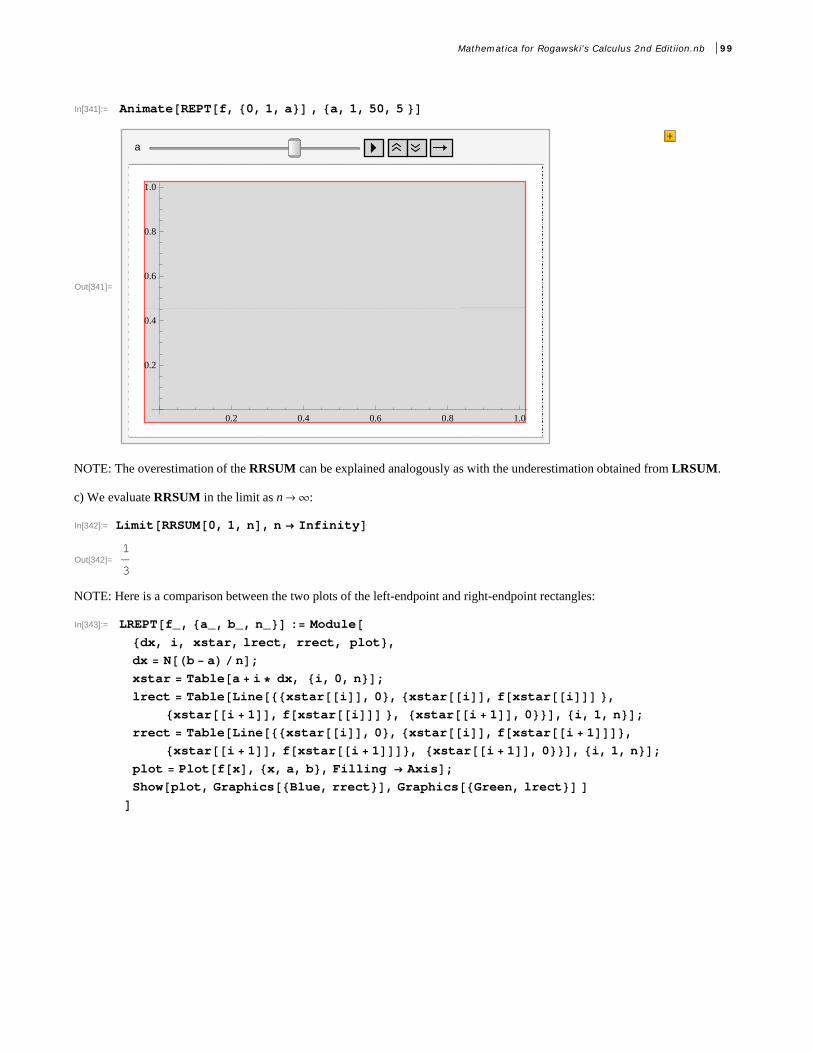
In[341]:= AnimateREPTf, 0, 1, a , a, 1, 50, 5

Out[341]=

a

0.2 0.4 0.6 0.8 1.0

0.2

0.4

0.6

0.8

1.0

NOTE: The overestimation of the RRSUM can be explained analogously as with the underestimation obtained from LRSUM.

c) We evaluate RRSUM in the limit as nØ¶:

In[342]:= LimitRRSUM0, 1, n, n Infinity

Out[342]=1

3

NOTE: Here is a comparison between the two plots of the left-endpoint and right-endpoint rectangles:

In[343]:= LREPTf_, a_, b_, n_ : Moduledx, i, xstar, lrect, rrect, plot,dx Nb a n;xstar Tablea i dx, i, 0, n;lrect TableLinexstari, 0, xstari, fxstari ,

xstari 1, fxstari , xstari 1, 0, i, 1, n;rrect TableLinexstari, 0, xstari, fxstari 1,

xstari 1, fxstari 1, xstari 1, 0, i, 1, n;plot Plotfx, x, a, b, Filling Axis;Showplot, GraphicsBlue, rrect, GraphicsGreen, lrect


In[344]:= fx_ : x2

LREPTf, 0, 1, 20

Out[345]=

In[346]:= fx_ : x2

AnimateLREPTf, 0, 1, a , a, 1, 100, 5

Out[347]=

a

0.2 0.4 0.6 0.8 1.0

0.2

0.4

0.6

0.8

1.0

ü 5.2.3 Riemann Sums Using Midpoints

The Riemann sum using the midpoints of each subinterval is given by the following formula. (We leave it to the student to verify

that the midpoint of ith subinterval is given by a + i + 1

2 b- a

n for i = 1, ..., n.)

In[348]:= ClearfMRSUMa_, b_, n_ : Sumfa i 1 2 b a n b a n, i, 1, n


1f x „ x by computing the Riemann sum relative to P using the midpoint method.


b) Plot the graph of f and the rectangles corresponding to the Riemann sum in part (a). c) Find the limit of the Riemann sum obtainded in part a) by letting nØ¶.

Solution: a) We evaluate

In[350]:= fx_ : x2

TableFormTablen, NMRSUM0, 1, n, n, 10, 100, 10,TableHeadings , "n", "Riemann Sum"


n Riemann Sum

10 0.442520 0.38562530 0.36768540 0.35890650 0.353760 0.35025570 0.34780680 0.34597790 0.344558100 0.343425

In[352]:= OptionsTableFormOut[352]= TableAlignments Automatic, TableDepth ,

TableDirections Column, TableHeadings None, TableSpacing Automaticb) Again, we can write a program that gives a plot of the rectangles corresponding to the Riemann sum in part (a) usingmidpoints.

In[353]:= MIDPTf_, a_, b_, n_ : Moduledx, i, xstar, mrect, plot,dx Nb a n;xstar Tablea i dx, i, 0, n;mrect

TableLinexstari, 0, xstari, fxstari xstari 1 2,xstari 1, fxstari xstari 1 2,xstari 1, 0, i, 1, n;

plot Plotfx, x, a, b, Filling Axis;Showplot, GraphicsRed, mrect


In[354]:= fx_ : x2

MIDPTf, 0, 1, 10

Out[355]=




In[356]:= fx_ : x2

AnimateMIDPTf, 0, 1, a , a, 1, 100, 5

Out[357]=

a

0.2 0.4 0.6 0.8 1.0

0.2

0.4

0.6

0.8

1.0

c) The limit of the Riemann sum using the midpoints is given by


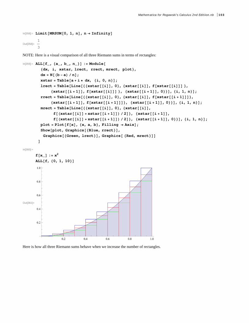
In[358]:= LimitMRSUM0, 1, n, n Infinity

Out[358]=1

3

NOTE: Here is a visual comparison of all three Riemann sums in terms of rectangles:

In[359]:= ALLf_, a_, b_, n_ : Moduledx, i, xstar, lrect, rrect, mrect, plot,dx Nb a n;xstar Tablea i dx, i, 0, n;lrect TableLinexstari, 0, xstari, fxstari ,

xstari 1, fxstari , xstari 1, 0, i, 1, n;rrect TableLinexstari, 0, xstari, fxstari 1,

xstari 1, fxstari 1, xstari 1, 0, i, 1, n;mrect TableLinexstari, 0, xstari,

fxstari xstari 1 2, xstari 1,fxstari xstari 1 2, xstari 1, 0, i, 1, n;

plot Plotfx, x, a, b, Filling Axis;Showplot, GraphicsBlue, rrect,GraphicsGreen, lrect, Graphics Red, mrect

In[360]:=

fx_ : x2

ALLf, 0, 1, 10

Out[361]=

Here is how all three Riemann sums behave when we increase the number of rectangles.


In[362]:= fx_ : x2

AnimateALLf, 0, 1, a , a, 1, 100, 5

Out[363]=

a

0.2 0.4 0.6 0.8 1.0

0.2

0.4

0.6

0.8

1.0

NOTE: All three limits from the left-endpoint, right-endpoint, and midpoint methods are equal. This is not surprising since each

is equal to 0

1x2 „ x (remember that the existence of a definite integral requires that all Riemann sums converge to the same limit).

However, the midpoint method tends to converge faster to the limit than the other two methods (discussed in your calculus text).

Example 5.7. Let f x = x3 + x2 + 1 on 0, 1 and let P = 0, 1 n, 2 n, ...., n n = 1 be a partition of 0, 1.a) Find the Riemann sum of f relative to P using the left endpoints of the partition.b) Find the Riemann sum of f relative to P using the right endpoints of the partition.c) Show that the difference between the two sums goes to 0 at nØ ¶. d) Find the limit of the Riemann sums in parts (a) and (b). Is this consistent with part (c)?e) What do you conclude from part (d)?

Solution: a) The Riemann sum using left endpoints is given by

In[364]:= ClearfLRSUMa_, b_, n_ : Sumfa i b a n Nb a n, i, 0, n 1

In[366]:= fx_ : x3 x2 1

LRSUM0, 1, n

Out[367]=5 12 n 19 n2

12 n2

b) The Riemann sum using right endpoints is given by

In[368]:= ClearfRRSUMa_, b_, n_ : Sumfa i b a n Nb a n, i, 1, n


In[370]:= fx_ : x3 x2 1

RRSUM0, 1, n

Out[371]=5 12 n 19 n2

12 n2

c) We now evaluate and simplify the difference between the two Riemann sums:

In[372]:= SimplifyRRSUM0, 1, n LRSUM0, 1, n

Out[372]=2

n

As n Ø¶, observe that this difference goes to zero.

d) Next, we use the limit command to evaluate the limit of the two Riemann sums:

In[373]:= LimitLRSUM0, 1, n, n Infinity

Out[373]=19

12

In[374]:= LimitRRSUM0, 1, n, n Infinity

Out[374]=19

12

In light of (c), we should not be surprised that the two limits are the same. After all, their difference was seen to converge to zero!

e) By definition of a definite integral, we conclude from (d) that 0

1x3 + x2 + 1 „ x = 19 12. We confirm this by evaluating

In[375]:= 0

1

x3 x2 1 x

Out[375]=19

12

ü Exercises

1. Let f x = x

x2+1for 0 § x § 1 and let P = 0 n, 1 n, 2 n, ... , n n = 1 be a partition of 0, 1.

a) Find the Riemann sum of f using the left endpoints of P and plot the rectangles that approximate the integral of f over 0, 1.Also, use the Animate command to see if the total area of the rectangles converges to the area of the region under the graph of fand above the x-axis.

b) Repeat (a) using right endpoints of P.

c) Repeat (a) using midpoints of P.

2. Let f x = x sin x on 0, p. Use a uniform partition P and repeat Exercise 1 (immediately above) for this function.

ü 5.3 The Fundamental Theorem of Calculus



The crowning achievement in calculus is the Fundamental Theorem of Calculus (FTC), which reveals that integration andantidifferentiation are equivalent. This can be expressed in two parts:

FTC - Part I: Given a continuous function f x on a, b, we have

ab

f x „ x = Fb - Fa.Here, Fx is any antiderivative of f x.FTC - Part II: If Fx = a

xf t „ t, then F ' x = f x.

NOTE: Physically the Fundamental Theorem of Calculus tells us that the area under a velocity curve of an object is the same asthe change in position of the object.

Mathematica naturally uses FTC to evaluate definite integrals whenever it is able to find an antiderivative. Of course, there areexamples where it is not able to do this, as the latter examples following demonstrate.

Example 5.8. Evaluate 15 x

2 x-1„ x.

Solution:

In[376]:= 1

5 x

2 x 1x

Out[376]=16

3

Example 5.9. Evaluate 3

2 x2-3

x„ x.

Solution:

In[377]:= IntegrateSqrtx^2 3 x, x, Sqrt3, 2

Out[377]= 1

2 3

In[378]:= NOut[378]= 0.0931003

Example 5.10. Approximate 0

1tan x2 „ x.

Solution: Here is an example of an integral that Mathematica cannot evaluate exactly but returns the integral unevaluatedbecause the precise answer is not expressible in terms of elementary functions.

In[379]:= IntegrateTanx^2, x, 0, 1

Out[379]= 0

1

Tanx2 x

However, a numerical approximation is still possible through the command N.


In[380]:= NOut[380]= 0.398414

Or we could use the command NIntegrate to perform both steps at once:

In[381]:= NIntegrateTanx^2, x, 0, 1Out[381]= 0.398414

Example 5.11. Use the fact that if m § f x §M for all x œ a, b, then mb - a § ab

f x „ x §M b - a to approximate

0

2x3 + 1 „ x.

Solution: We note that the function f x = x3 + 1 is increasing on 0, 2. This can be checked by finding f ' x and observing

that f ' x > 0 for all x (or by simply drawing the graph of f ). Thus, 1 = f 0 § f x § f 2 = 3 and so

1 2 - 0 § 02

1 + x3 „ x § 3 2 - 0 or

2 § 0

21 + x3 „ x § 6

We can confirm this by evaluating

In[382]:= Integrate x3 1 , x, 0, 2

Out[382]= 2 Hypergeometric2F1 12,1

3,4

3, 8

Since the function Hypergeometric2F1 is not known to us, we use

In[383]:= NIntegrate x3 1 , x, 0, 2Out[383]= 3.24131

Example 5.12. Let f x = cosx2 on 0, 2 and define gx = 0

xf t „ t = 0

xcost2 „ t.

a) Plot the graph of f .b) Find the value(s) of x for which gx) starts to decrease.c) Estimate gx for x = 0.2, 0.4, 0.6, 0.8, 1.0, 1.2, 1, 4, 1.6, 1.8, 2.d) Draw the graphs of gx and g ' x.e) How do the graphs of f x and g ' x compare?

Solution: a) We plot the graph of f .


In[384]:= Clearffx_ Cosx2gx_

0

x

ft t

Out[385]= Cosx2

Out[386]=

2FresnelC 2

x

NOTE: The function FresnelC is called the Fresnel Cosine function and plays an important role in physics and engineering. TheFresnel Sine function is defined in the obvious manner.

In[387]:= Plotfx, x, 0, 2

Out[387]=0.5 1.0 1.5 2.0

-1.0

-0.5

0.5

1.0

b) We note that the graph of f is above the x-axis (positive area) for x between 0 and p 2 and below the x-axis for x between

p 2 and 2. Thus, the graph of g starts to decrease after p 2 . The following table of the Riemann sums of f on 0, x (for xvarying from 0 to 2) shows this point.

In[388]:= fx_ : x2

TableFormTablen, NMRSUM0, 1, n, n, 10, 100, 10


10 0.442520 0.38562530 0.36768540 0.35890650 0.353760 0.35025570 0.34780680 0.34597790 0.344558100 0.343425

In[390]:= LRSUMa_, b_, n_ : Sumfa i b a n Nb a n, i, 0, n 1


In[391]:= TableFormTablex, LRSUM 0, x, 100, x, 0, 2, 0.1,TableHeadings , "x", "Riemann Sum"


x Riemann Sum

0. 0.0.1 0.000328350.2 0.00262680.3 0.008865450.4 0.02101440.5 0.04104380.6 0.07092360.7 0.1126240.8 0.1681150.9 0.2393671. 0.328351.1 0.4370341.2 0.5673891.3 0.7213851.4 0.9009921.5 1.108181.6 1.344921.7 1.613181.8 1.914941.9 2.252152. 2.6268

NOTE: Since g is the integral, it should start to decrease at x = p 2 º 1.25. We can confirm this by examining the values of gin the neighborhood of this point:

In[392]:= Tablex, LRSUM 0, x, 100, x, 1.2, 1.3, 0.01 TableForm


1.2 0.5673891.21 0.5816921.22 0.5962341.23 0.6110161.24 0.626041.25 0.6413091.26 0.6568231.27 0.6725871.28 0.68861.29 0.7048651.3 0.721385

From the table above, we see that the function g does indeed start to decrease at approximately x = 1.25:

c) Here is the table of values for gx:


In[393]:= TableFormTablex, gx, x, 0.2, 2, 0.2Out[393]//TableForm=

0.2 0.1999680.4 0.3989770.6 0.5922710.8 0.7678481. 0.9045241.2 0.9739451.4 0.9497791.6 0.8255171.8 0.6353652. 0.461461

d) The graphs of the function f x and g ' x are given below:

In[394]:= Plotgx, g'x, x, 0, 2, PlotStyle Red, Blue

Out[394]=0.5 1.0 1.5 2.0

-1.0

-0.5

0.5

1.0

e) The graphs of the function f x and g ' x are given below:

In[395]:= Plotfx, g'x, x, 0, 2, PlotStyle Red, Blue

Out[395]=

0.5 1.0 1.5 2.0

-1

1

2

3

4

This means that the two graphs are the same. In fact, from the Fundamental Theorem of Calculus, we know that g ' x = f x.

ü Exercises

In Exercies 1 troough 11, evalaute the given integrals.

1. 01x2 + 2 „ x 2. 0

pcos 3 x „ x 3. 0

11 - x2 „ x 4. -pp sin 2 x „ x


5. 0

3x3 - 4 x2 + x d x6. 1

4 1

x+ 2 x d x 7. 0

p

4 sec x d x 8. 0

2

4 2

1-4 x2

d x

9. 03 1

x+1d x 10. 1

4 1

x+ 2 x2 d x 11. 0

pex sin x d x

12. Let Sx = 0

xsin 1

2p t2 „ t (Sx is called the Fresnel sine)

a) Plot the graph of S and approximate the value of S as xØ¶. Confirm your approximation by evaluating the limit as xØ ¶.

b) Find S ' x and use it to find the interval(s) on whcih Sx increase and decrease. Hint: Apply the Fundamental Theorem ofCalculus.

c) On what intervals is S concave up? Concave down?

d) Find the value of x for which Sx = 0.7.

13. Find an explicit formula for a continuous function f such that

0

xf t „ t = x ex + 0

x f t2 t2+1

„ t.

(Hint: First take the derivative of both sides and then solve for f x.)

ü 5.4 Integrals Involving Trigonometric, Exponential, and Logarithmic Functions

In your calculus text, you will learn how to evaluate integrals using different techniques. In Mathematica, we do not need tospecify the technique. It chooses the technique appropriate for the problem. However, there are some integrals that cannot beevaluated in terms of elementary functions. In such cases, Mathematica will return the integal unevaluated or gives us a name forthe integral.

Below, we will consider some examples of integrals that involve trigonometric functions, exponential, and logarithmic functions.If done by hand, some of these integrals require integration by parts, partial fraction decompositions, or trigonometric substitu-tions.

Example 5.13. Evaluate x2

x3+12„ x.

Solution: If done by hand, this integral involves using the substitution method.

In[396]:= Integratex^2 x^3 1^2, x

Out[396]= 1

3 1 x3

Example 5.14. Evaluate x5+x2+x+2

x2-1„ x.

Solution: This integral involves long division and partial fraction decomposition.


In[397]:= x5 x2 x 2

x2 1x

Out[397]= x x2

2x4

45

2Log1 x 1

2Log1 x

Example 5.15. Evaluate x4+x3+x+1

x2+12„ x.

Solution: This integral involves long division, partial fraction decomposition, and inverse trigonometric functions.

In[398]:= x4 x3 x 1

x2 12x

Out[398]= x x

1 x2 ArcTanx 1

2Log1 x2

NOTE: All functions that appear as output are written in Mathematica's notation. To convert the output to a more familiar form

the command TraditionalForm can be used. Here is the "traditional" form of the output below (note that log x means the sameas ln x in this case).

In[399]:= x4 x3 x 1

x2 12x TraditionalForm

Out[399]//TraditionalForm=

x

x2 + 1+

1

2logx2 + 1 + x - tan-1x

Example 5.16. Evaluate x2 sin x „ x.

Solution: This integral involves integration by parts (twice).

In[400]:= x2 Sinx x

Out[400]= 2 x2 Cosx 2 x Sinx

Example 5.17. Evaluate -1

1-x2

„ x.

Solution: This integral involves trigonometric substitution.

In[401]:= Integrate1 Sqrt1 x^2, xOut[401]= ArcSinxNOTE: Your calculus textbook may give arccos x for the answer, as opposed to -arcsin x as above. Can you explain how theintegration constant resolves the difference in these two answers?

Here are some examples of integrals that are important in applications but do not have an elementary antiderivative.


In[402]:= Sinx2 x

Out[402]=

2FresnelS 2

x

In[403]:= Ex2x

Out[403]=1

2 Erfx

In[404]:= IntegrateSinx x, xOut[404]= SinIntegralxWe can use NIntegrate to evaluate these integrals over any finite interval. For example:

In[405]:= NIntegrateEx2, x, 0, 10Out[405]= 0.886227

In[406]:= NIntegrateLogx x, x, 2, 100Out[406]= 10.3636

Example 5.18. Let fnx = 1

xtn „ t . Investigate the limit graphically by plotting fnx) for n = 0, –0 .3, –0 .6, and –0 .9 together

with gx = ln x on a single plot.

In[407]:= Clearf, ggx_ : Logxfx_, n_ :

1

x

tn t

In[410]:= Plotfx, n . n 0, 0.3, .6, .9, gx, x, 0, 10, PlotStyle Red, Blue

Out[410]=

2 4 6 8 10

-4

-2

2

4

6

8

ü Exercises

In Exercises 1 though 5, evaluate the given integral.


1. x 2 - x „ x 2. x3 1 + x2 „ x 3. tan2 x sec4 x „ x

4. x2-2 x-1

x3+x„ x 5. x-1

x2+x-1

„ x

In Exercises 6 through 11, use various values of a, b, and n to evaluate the given integral. Then make a conjecture for a generalformula and prove your conjecture.

6. 1

x+a x+b „ x 7. cos a x sinb x „ x 8. xn ln x „ x

9. xn ex „ x 10. xn sinx „ x 11. ea x cosb x „ x


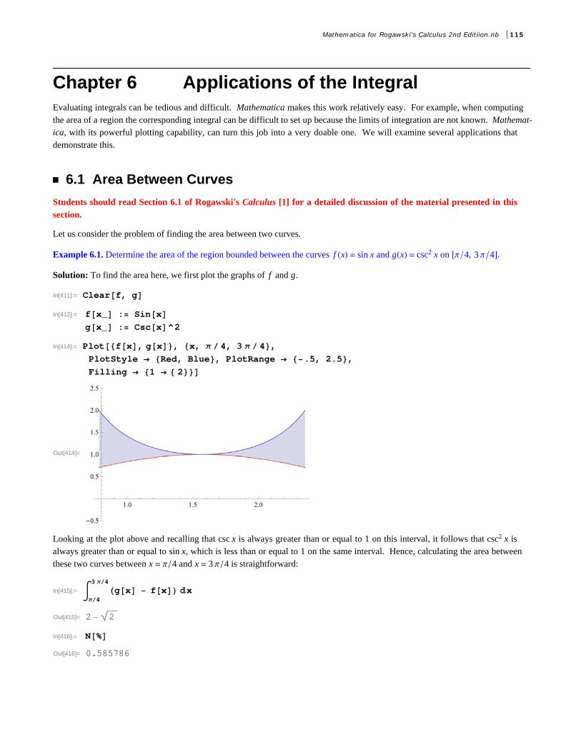
Chapter 6 Applications of the IntegralEvaluating integrals can be tedious and difficult. Mathematica makes this work relatively easy. For example, when computingthe area of a region the corresponding integral can be difficult to set up because the limits of integration are not known. Mathemat-ica, with its powerful plotting capability, can turn this job into a very doable one. We will examine several applications thatdemonstrate this.

ü 6.1 Area Between Curves


Let us consider the problem of finding the area between two curves.

Example 6.1. Determine the area of the region bounded between the curves f x = sin x and gx = csc2 x on p 4, 3 p 4.Solution: To find the area here, we first plot the graphs of f and g.

In[411]:= Clearf, gIn[412]:= fx_ : Sinx

gx_ : Cscx^2In[414]:= Plotfx, gx, x, 4, 3 4,

PlotStyle Red, Blue, PlotRange .5, 2.5,Filling 1 2

Out[414]=

Looking at the plot above and recalling that csc x is always greater than or equal to 1 on this interval, it follows that csc2 x isalways greater than or equal to sin x, which is less than or equal to 1 on the same interval. Hence, calculating the area betweenthese two curves between x = p 4 and x = 3 p 4 is straightforward:

In[415]:= 4

3 4gx fx x

Out[415]= 2 2

In[416]:= NOut[416]= 0.585786


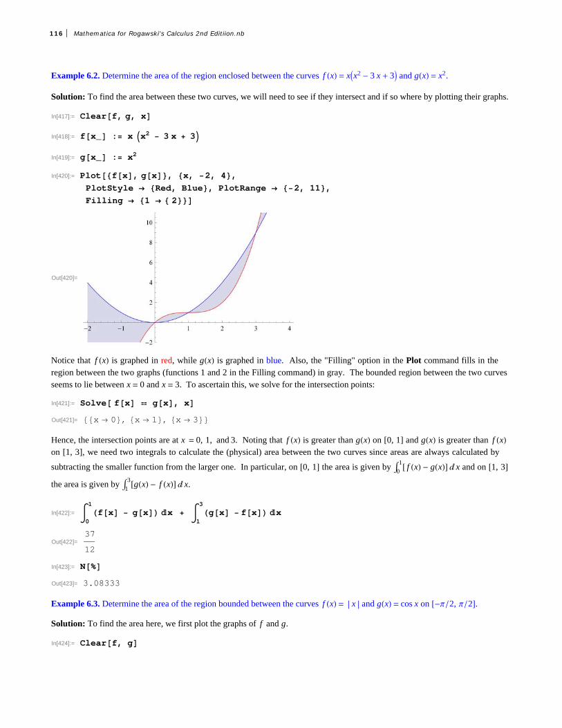
Example 6.2. Determine the area of the region enclosed between the curves f x = xx2 - 3 x + 3 and gx = x2.

Solution: To find the area between these two curves, we will need to see if they intersect and if so where by plotting their graphs.

In[417]:= Clearf, g, xIn[418]:= fx_ : x x2 3 x 3In[419]:= gx_ : x2

In[420]:= Plotfx, gx, x, 2, 4,PlotStyle Red, Blue, PlotRange 2, 11,Filling 1 2

Out[420]=

Notice that f x is graphed in red, while gx is graphed in blue. Also, the "Filling" option in the Plot command fills in theregion between the two graphs (functions 1 and 2 in the Filling command) in gray. The bounded region between the two curvesseems to lie between x = 0 and x = 3. To ascertain this, we solve for the intersection points:

In[421]:= Solve fx gx, xOut[421]= x 0, x 1, x 3Hence, the intersection points are at x = 0, 1, and 3. Noting that f x is greater than gx on [0, 1] and gx is greater than f xon [1, 3], we need two integrals to calculate the (physical) area between the two curves since areas are always calculated by

subtracting the smaller function from the larger one. In particular, on 0, 1 the area is given by 0

1 f x - gx „ x and on 1, 3the area is given by 1

3gx - f x „ x.

In[422]:= 0

1

fx gx x 1

3

gx fx x

Out[422]=37

12

In[423]:= NOut[423]= 3.08333

Example 6.3. Determine the area of the region bounded between the curves f x = x and gx = cos x on -p 2, p 2.Solution: To find the area here, we first plot the graphs of f and g.

In[424]:= Clearf, g


In[425]:= fx_ : Absxgx_ : Cosx

In[427]:= Plotfx, gx, x, 2, 2,PlotStyle Red, Blue, PlotRange 1, 2,Filling 1 2

Out[427]=

From the picture above, we will need to consider the total area as a sum of three separate regions. To this end, we first find the

intersection points of these two curves in order to obtain the limits of integration. Make note of the fact that the Solve command

does not work here because it is only able to solve algebraic equations. Instead, we use the FindRoot command to solve theequation f x - gx = 0 using an initial guess of x = 0.75 (based on the plot above):

In[428]:= FindRootfx gx, x, 0.75Out[428]= x 0.739085Thus our root is approximately x = 0.739085. By symmetry we see there is another root at x = -0.739085. Hence, the areabetween these two curves is the sum of the three integrals:

In[429]:= 2

0.739085

fx gx x 0.739085

0.739085

gx fx x 0.739085

2fx gx x

Out[429]= 2.06936

Hence the area of our bounded region is 2.06936.

NOTE: Observe that our region is symmetric about the y-axis and thus the same answer could have been found by computing thearea of only half the region (the right half, say) and doubling the result.

ü Exercises

1. Find the area between the curves y = sin x and y = sin 2 x between x = 0 and x = p.

2. Find the area between the graphs of x = sin y and x = 1 - cos y between y = 0 and y = p 2.

3. Find the area above y = 1 - x p and below y = sin x.

ü 6.2 Average Value



Remember that the average value of a function f x on a, b is defined as

fave =1

b-a a

bf x „ x.

Related to this notion is the Mean Value Theorem for Integrals (MVTI), which states that for any continuous function f x ona, b there exists a value c œ a, b such that

f c = fave.

Example 6.4. Let f x = 2 cos x - x.a) Find the only positive root a of f .b) Calculate the average value of f on 0, a.c) Determine a value c that satisfies the Mean Value Theorem for Integrals on 0, a.Solution:

a) To calculate a, we first plot the graph of f and then use the FindRoot command with x = 1 as our initial guess:

In[430]:= ClearfIn[431]:= fx_ : 2 Cosx x

In[432]:= Plotfx, x, ,

Out[432]=

-3 -2 -1 1 2 3

-5

-4

-3

-2

-1

1

2

In[433]:= root FindRootfx, x, 1Out[433]= x 1.02987Therefore, a = 1.02987 accurate to 5 decimal places.

b) We next calculate the average value of f on 0, a:In[434]:= root1, 2Out[434]= 1.02987

In[435]:= fave 1

00

fx x

Out[435]= 1.14981

Thus, the average value is approximately fave = 1.14981.

c) By MVTI, there exists a value c œ 0, a such that f c = fave. To find c, we solve this equation for c, or equivalently,

f c - fave = 0.


In[436]:= FindRootfc fave, c, .5Out[436]= c 0.55256

ü Exercises

1. Which of f x = x sin2 x and gx = x2 sin2 x has a larger average value over 0, 2? Over 2, 4?2. Let fave denote the average value of f x = x3 + x2 + 5 on 0, 4. Find a value for c inside 0, 4 such that f c = fave.

ü 6.3 Volume of Solids of Revolution


We recall that a definite integral can be evaluated by employing the definition

a

bf x „ x = lim

nØ+¶i=1

n f xi*D xi.

Another application of the definite integral involves finding the volume of a solid of revolution, that is, a solid obtained byrevolving a region in the plane about one of the coordinate axes.

ü 6.3.1 The Method of Discs

Let S be a solid of revolution obtained by revolving the region bounded by the graphs of y = f x, y = 0, and the vertical linesx = a and x = b, about the x-axis. To obtain the volume of S, we can approximate S by discs, i.e., cylinders obtained by revolv-ing each rectangle, constructed by a Riemann sum of f relative to a partition P = x0, x1, x2, .... , xn of a, b, about the x-axis.Using the fact that the volume of a cylinder with radius R and height h is given by

V = p R2 h,

it follows that the volume of the ith cylinder (corresponding to the ith rectangle) is Vi = p f xi*2 D x. Hence, an approximation

to the volume of S is given by the Riemann sum

VolS ºi=1n Vi = pi=1

n f xi*2 D x.

In the limit as nØ¶, we obtain the exact volume of S:

VolS = p limnØ¶i=1n f xi

*2 D x = p a

b f x2 „ x.

NOTE: If the region is revolved about the y-axis, then the volume of S is given by

VolS = p cd f y2 „ y.

Example 6.5. Find the volume of the solid of revolution obtained by rotating the region bounded by the graph of f x = x , thex-axis, and the vertical line x = 3.

Solution: We define f x in Mathematica and illustrate both the region and rectangles that are rotated to obtain the solid anddiscs, respectively. For this, we recall our program from Chapter 5 of this manual that was used to draw these rectangles.


In[437]:= LEPTf_, a_, b_, n_ : Moduledx, k, xstar, lrect, plot,dx Nb a n;xstar Tablea i dx, i, 0, n;lrect TableLinexstari, 0, xstari, fxstari ,

xstari 1, fxstari , xstari 1, 0, i, 1, n;plot Plotfx, x, a, b, Filling Axis;Showplot, GraphicsGreen, lrect

In[438]:= fx_ : x

plot LEPTf, 0, 3, 20

Out[439]=

The plot above shows our region shaded in gray and our rectangles outlined in green. We now rotate this shaded region about

the x-axis to obtain a solid of revolution called a paraboloid. This is achieved in Mathematica using the Revolution-

Plot3D[{f,x},{x,a,b}] command, which generates a surface of revolution having radius f at height x. This means that the verticalaxis shown in the plot below is actually the x-axis.


In[440]:= S RevolutionPlot3D x , x, x, 0, 3

Out[440]=

The exact volume of the paraboloid is then given by

In[441]:= V 0

3

fx2 x

Out[441]=9

2

ü 6.3.2 The Method of Washers

For a solid of revolution S generated by revolving a region bounded between two curves f x and gx on a, b about the x-axis,we employ washers (rings) instead of discs. Refer to your calculus textbook for a detailed treatment. The corresponding volumeof S is given by (let's assume gx ¥ f x)

VolS = p a

bgx2 - f x2 „ x.

Example 6.6. Find the volume of the solid generated by revolving about the x-axis the region enclosed by the parabola y = x2 + 1and the straight line y = x + 3.

Solution: Our initial goal is to find the points of intersection and secure the limits of integration.

In[442]:= Clearf, g, xfx_ : x2 1

gx_ : x 3


In[445]:= Plotfx, gx, x, 2, 4, PlotStyle Red, Blue,PlotRange 2, 8, Filling 1 2

Out[445]=

We notice that f x is graphed in red, while gx is graphed in blue. The following command solves for their intersection points:

In[446]:= Solvefx gx, xOut[446]= x 1, x 2One can easily verify that the intersection points are -1, 2 and 2, 5. Thus, our limits of integration are x = -1 and x = 2.

Let P and Q denote the solids of revolution by revolving each of the regions lying under f and g, respectively, along the interval-1, 2. Our solid S, obtained by rotating the region between f and g on -1, 2 about the x-axis, can then be viewed as thedifference of Q and P, i.e., the solid Q with the solid P removed from it. Following are surface plots of the three solids P, Q, andS. Again, note that the vertical axis shown in each of the plots below is actually the x-axis.


In[447]:= P RevolutionPlot3Dfx, x, x, 1, 2, AspectRatio AutomaticQ RevolutionPlot3Dgx, x, x, 1, 2, AspectRatio Automatic

Out[447]=

Out[448]=


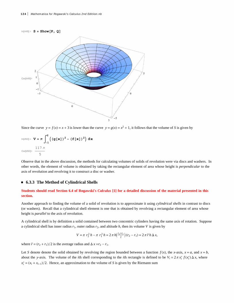
In[449]:= S ShowP, Q

Out[449]=

Since the curve y = f x = x + 3 is lower than the curve y = gx = x2 + 1, it follows that the volume of S is given by

In[450]:= V 1

2

gx2 fx2 x

Out[450]=117

5

Observe that in the above discussion, the methods for calculating volumes of solids of revolution were via discs and washers. Inother words, the element of volume is obtained by taking the rectangular element of area whose height is perpendicular to theaxis of revolution and revolving it to construct a disc or washer.

ü 6.3.3 The Method of Cylindrical Shells


Another approach to finding the volume of a solid of revolution is to approximate it using cylindrical shells in contrast to discs(or washers). Recall that a cylindrical shell element is one that is obtained by revolving a rectangular element of area whoseheight is parallel to the axis of revolution.

A cylindrical shell is by definition a solid contained between two concentric cylinders having the same axis of rotation. Supposea cylindrical shell has inner radius r1, outer radius r2, and altitude h, then its volume V is given by

V = p r22 h - p r1

2 h = 2 p h r2+r1

2 r2 - r1 = 2 p r hD x,

where r = r2 + r1 2 is the average radius and D x =r2 - r1.

Let S denote denote the solid obtained by revolving the region bounded between a function f x, the x-axis, x = a, and x = b,about the y-axis. The volume of the ith shell corresponding to the ith rectangle is defined to be Vi = 2 p xi

* f xi*D x, where

xi* = xi + xi-1 2. Hence, an approximation to the volume of S is given by the Riemann sum


VolS ºi=1n Vi = 2 pi=1

n xi* f xi

*D x.

In the limit as nØ¶, we obtain the exact volume of S:

VolS = 2 p limnØ¶i=1n xi

* f xi*D x = 2 p a

bx f x „ x.

NOTE: If the region is revolved about the x-axis using cylindrical shells, then the volume of S is given by

VolS = 2 p c

dy f y „ y.

Example 6.7. Consider the region bounded by the curve y = x2, the x-axis, and the line x = 2. Find the volume of the solidgenerated by revolving this region about the y-axis using the method of cylindrical shells.

Solution: Let us first plot the region bounded by the given curves (shaded in the plot below):

In[451]:= fx_ x^2;

Plotfx, x, 0, 2, Filling Axis

Out[452]=

We then revolve this shaded region about the y-axis to obtain our solid S (parabolic bowl). This can be seen in the three plotsfollowing, which illustrate S as the difference of the solids Q (cylinder) and P (paraboloid), that is, Q with P removed from it.


In[453]:= P RevolutionPlot3Dfx , x, 0, 2Q RevolutionPlot3D2, y , y, 0, 4

Out[453]=

Out[454]=


In[455]:= S ShowP, Q

Out[455]=

The volume of S is given by

In[456]:= V 2 0

2

x fx xOut[456]= 8

NOTE: The volume in this example can also be calculated using the washer method. However, one would first have to solve the

equation y = x2 for x, yielding x = y . Moreover, the limits of integration (with respect to y) would have to be determined,which in this case would be y = 0 and y = 4 corresponding to x = 0 and x = 2, respectively. Hence,

In[457]:= V 0

4

22 y 2

y

Out[457]= 8

The two answers from both methods agree as they should.

Example 6.8. Sketch the ellipse x2

a2+

y2

b2= 1 and find the volume of the solid obtained by revolving the region enclosed by the

ellipse about the x-axis.

Solution: We will use the ContourPlot command to plot the ellipse for a = 2 and b = 3. The reader should experiment withother values of a and b.


In[458]:= a 2;

b 3;

ContourPlot x2

a2y2

b2 1, x, a 1, a 1, y, b 1, b 1,

AspectRatio Automatic, Axes True, Frame False

Out[460]=-3 -2 -1 1 2 3

-4

-2

2

4

To plot the corresponding solid of revolution (ellipsoid), we first solve x2

a2+

y2

b2= 1 for y.

In[461]:= Cleara, b

sol Solvex2

a2y2

b2 1, y

Out[462]= y b a2 x2

a, y

b a2 x2

a

The positive and negative solutions above correspond to the upper half and lower half, respectively, of the ellipse. We shallconsider the upper half in plotting the ellipsoid and computing its volume by defining

f x = b2 - b2 x2

a2= b 1 - x2

a2.

In[463]:= fx_ sol2, 1, 2

Out[463]=b a2 x2

a

Here is a plot of S (rotated 90 degrees about the x-axis).


In[464]:= a 2;

b 3;RevolutionPlot3Dfx, x , x, a, a

Out[466]=

To find the volume of the ellipsoid, we can employ either method, disc or shell, but in this case the disc method is preferable

from a computational standard. This is because the disc formula for volume contains the square term f x2, which lets us avoidhaving to deal with radical terms if the shell method were used. Since the ellipsoid is defined along the integral -a, a, itsvolume based on the disc method is therefore

In[467]:= V a

a

fx2 xOut[467]= 24

More generally, the volume of the ellipsoid for arbitrary positive values of a and b is given by

In[468]:= Cleara, bV

a

a

fx2 x

Out[469]=4

3a b2

Thus, V = 4

3p a b2.

NOTE: If we let a = b, then the ellipsoid becomes a sphere and the formula above reduces to the classic formula V = 4

3p a3,

where a is the radius of the sphere.

ü Exercises

1. Plot the solid of revolution obtained by rotating the region enclosed by the graphs about the given axis and calculate itsvolume.


a) y = 9

x2, y = 10 - x2 about the x-axis

b) y = 16 - x4, y = 0, x = 2, x = 3 about the y -axis

2. Plot the hypocycloid x23 + y23 = 1 and find the volume of the solid obtained by revolving the region enclosed by the hypocy-cloid about the y-axis. Is the volume of the solid obtained by revolving the same region about the x-axis the same? Justify your

answer. (Hint: Use the ContourPlot command.)

3. Use the Shell Method to find the volume of the solid obtained by rotating the region enclosed by the graphs in each part belowabout the y-axis.a) y = x2, y = 8 - x2, and x = 0

b) y = 1

2x2and y = sinx2

4. The solid generated by revolving the region between the two branches of the hyperbola y2 - x2 = 1 from x = -a to x = a aboutthe x-axis is called a hyperboloid. Find the volume of the hyperboloid for a = 2 and then for any arbitrary value of a.


Chapter 7 Techniques of Integration

ü 7.1 Numerical Integration

Students should read Section 7.1 of Rogawski’s Calculus [1] for a detailed discussion of the material presented in thissection.

Numerical integration is the process of approximating a definite integral using appropriate sums of function values. We already

saw in Chapter 5 of this text formulas for Right, Left, and Midpoint Rules and their subroutines LRSUM, RRSUM, and

MRSUM, respectively. In this section, we will develop two additional rules: the Trapezoidal Rule and Simpson’s Rule.

ü 7.1.1 Trapezoidal Rule

The Trapezoidal Rule approximates the definite integral a

bf x „ x by using areas of trapezoids and is given by the formula:

Tn = .5 b - a n y0 + 2 y1 + ... + 2 yn-1 + ynwhere n is the number of trapezoids and yi = f a + i b - a n . This formula can be found in your calculus text. Here is a

Mathematica subroutine, called TRAP, for implementing the Trapezoidal Rule:

In[470]:= Clearf, a, b, nIn[471]:= TRAPa_, b_, n_ :

fa 2 Sumfa i b a n, i, 1, n 1 fb .5 b a nExample 7.1. Calculate the area under the function f x = x2 on 0, 1 using the Trapezoidal Rule for various values of n.

Solution: The following output gives a table of approximations of 0

1x2 „ x based on the Trapezoidal Rule for n = 10, 20, ..., 100.

In[472]:= fx_ : x2

TableFormTablen, NTRAP0, 1, n, n, 10, 100, 10,TableHeadings , "n", " Tn"


n Tn

10 0.33520 0.3337530 0.33351940 0.33343850 0.333460 0.3333870 0.33336780 0.33335990 0.333354100 0.33335

It is clear that these values are converging to 1/3, which is the exact value of our definite integral:


In[474]:= 0

1

x2 x

Out[474]=1

3

ü 7.1.2 Simpson’s Rule

One difference between Simpson’s Rule and all the other rules we have developed so far (TRAP, LRSUM, RRSUM, and

MRSUM) is that the number of partition points, n, in this case, must be even. The other difference is that Simpson’s Rule is aquadratic approximation based on parabolas, whereas the other rules are linear approximations based on lines. The formula forSimpson’s Rule is given by (refer to your calculus text for details):

Sn = 1 3 y0 + 4 y1 + 2 y2 + 4 y3 + 2 y4 + ... + 4 yn-3 + 2 yn-2 + 4 yn-1 + yn b - a n = 1 3y0 + 4 y1 + y2 + y2 + 4 y3 + y4 + ... + yn-2 + 4 yn-1 + yn b - a n

where yi = f a + i b - a n. Here is a Mathematica subroutine, called SIMP, for implementing Simpson’s Rule:

In[475]:= Cleara, b, nIn[476]:= SIMPa_, b_, n_ :

1 3 Sumfa 2 i 2 b a n 4 fa 2 i 1 b a n

fa 2 i b a n, i, 1, n 2 b a nExample 7.2. Calculate the area under the function f x = x2 on 0, 1 using Simpson’s Rule for various values of n.

Solution: We use the same set of values of n as in the previous example. This will allow us to compare Simpson’s Rule with theTrapezoidal Rule.

In[477]:= fx_ : x2

TableFormTablen, NSIMP0, 1, n, n, 10, 100, 10,TableHeadings , "n", " sn"


n sn

10 0.33333320 0.33333330 0.33333340 0.33333350 0.33333360 0.33333370 0.33333380 0.33333390 0.333333100 0.333333

Notice how fast SIMP converges to the actual value of the integral (1/3) compared to TRAP.

Example 7.3. Calculate the definite integral of f x = sin25 x2 on 0, 1 using Simpson’s Rule and approximate it to five

decimal places. What is the minimum number of partition points needed to obtain this level of accuracy?

Solution: We first evaluate SIMP using values for n in increments of 20.


In[479]:= fx_ : Sin25 x2TableFormTablen, NSIMP0, 1, n, n, 20, 200, 20,TableHeadings , "n", " sn"


n sn

20 0.095894340 0.1052660 0.10552680 0.105566100 0.105576120 0.10558140 0.105582160 0.105582180 0.105583200 0.105583

Based on the output our approximation, accurate to five decimal places, is 0.10558. This first occurs between n = 100 to n = 120.We evaluate SIMP inside this range to zoom in on the minimum number of partition points needed.

In[481]:= fx_ : Sin25 x2TableFormTablen, NSIMP0, 1, n, n, 100, 120, 2,TableHeadings , "n", " sn"


n sn

100 0.105576102 0.105577104 0.105577106 0.105578108 0.105578110 0.105579112 0.105579114 0.105579116 0.10558118 0.10558120 0.10558

Thus, we see that the minimum number of points needed is n = 116. How does this compare with the minimum number of pointsneeded by TRAP to obtain the same level of accuracy?

NOTE: Observe that SIMP does not converge as fast in this example as in the previous example. This is because the functionf x = sin25 x2 is oscillatory as the following graph demonstrates:


In[483]:= Plotfx, x, 0, 1

Out[483]=0.2 0.4 0.6 0.8 1.0

-1.0

-0.5

0.5

1.0

Try increasing the frequency of this function, say to sin100 x2, to see how well SIMP performs.

ü 7.1.3 Midpoint Rule

Since most calculus texts include again the Midpoint Rule in the section on numerical integration, for completeness, we will too.The Riemann sum using the midpoints of each subinterval is given by the following formula:

In[484]:= ClearfMRSUMa_, b_, n_ : Sumfa i 1 2 b a n b a n, i, 1, n

Example 7.4. Calculate the area under the function f x = x2 on 0, 1 using the Midpoint Rule for various values of n.

Solution:

In[486]:= fx_ : x2

TableFormTablen, NMRSUM0, 1, n, n, 10, 100, 10,TableHeadings , "n", "Midpoint rule"


n Midpoint rule

10 0.332520 0.33312530 0.33324140 0.33328150 0.333360 0.3333170 0.33331680 0.3333290 0.333323100 0.333325

ü Exercises

1. Consider the definite integral 1

2lnx „ x.

a) Using the Trapezoidal Rule, Simpson's Rule, and Midpoint Rule, approximate this integral for n = 10, 20, ..., 100.

b) Compare how fast each subroutine (TRAP, SIMP, MRSUM) converges to ablnx „ x and decide which of these rules is

"best."


2. Repeat Exercise 1 for the following definite integrals:

a) 02 ex

x+1„ x b) 0

1cosx2 „ x c) 0

1ex2

„ x

Can you make any general conclusions about which rule (Trapezoidal, Simpson’s, Midpoint) is best?

3. For each of the functions given below, set up a definite integral for the volume of the solid of revolution obtained by revolving

the region under f x along the given interval and about the given axis. Then use the subroutines TRAP, SIMP, and MRSUMto approximate the volume of each solid accurate to two decimal places (use various values of n to obtain the desired accuracy).

a) f x = cos x; 0, p 2; x-axis b) f x = e-x2; 0, 1; y-axis c) f x = sin x, 0, p, x - axis

ü 7.2 Techniques of Integration

Students should read Sections 7.2 trhough 7.4 and 7.6 of Rogawski's Calculus [1] for a detailed discussion of the materialpresented in this section.

All calculus texts have at least a chapter devoted to "Techniques of Integration." When using Mathematica, these techniques areusually not necessary since Mathematica automatically gives you the answer.

ü 7.2.1 Substitution

On occasion, we do need to use techniques of integration, even when using Mathematica.

Example 7.5. Evaluate the following integral: 2x 2x2 - 1 „ x.

Solution: We evaluate this integral in Mathematica:

In[488]:= 2x 2x2 1 x

Out[488]=

2x 1 4x Log2x 1 4x Log4

To students in a first-year calculus course, this answer makes no sense. There are many integrals that Mathematica cannotevaluate at all, or cannot evaluate in terms of elementary functions (such as the integral above). Some of these integrals aredoable in terms we should understand, once we first use an appropriate technique of integration. In the above example, all weneed to do is first make the following substitution: u = 2x and d u = ln 2 2x d x, which transforms the integral to:

In[489]:=1

Log2 u2 1 u

Out[489]=

12u 1 u2 1

2Logu 1 u2

Log2This is the correct answer. All we need to do is substitute 2x for u, and add the arbitrary constant of integration, getting:

1

2 Log2 ( 2x -1 + 2x2 - Log[2x + -1 + 2x2 ] ) + C

Note that the Mathematica function Log[x] is equivalent to the standard form ln x.

ü 7.2.2 Trigonometric Substitution


Example 7.6. Evaluate 1

x2 x2-9

„ x.

Solution: By hand, the integral 1

x2 x2-9

„ x would normally be evaluated with a trigonometric substitution of the form

x = 3 secq. But with Mathematica, we can do this directly:

In[490]:= 1

x2 x2 - 9

‚ x

Out[490]=9 x2

9 x

This, of course, is the correct answer, when we remember that Mathematica does not add an arbitrary constant to indefiniteintegrals.

ü 7.2.3 Method of Partial Fractions

Integrals of rational expressions often require the Method of Partial Fraction Decomposition to evaluate them (by hand). Forexample:

3 x-3

x2+5 x+4„ x = 5

x+4- 2

x+1 „ x = 5 ln x + 4 -2 ln x + 1 = ln

x+45

x+12

On the other hand, Mathematica will give us essentially the same answer for this integral, but does its work behind the sceneswithout revealing its technique:

In[491]:= Simplify3 x 3

x2 5 x 4x

Out[491]= 2 Log1 x 5 Log4 x

If we would like to see the partial fraction decomposition of the integrand, 3 x-3

x2+5 x+4, Mathematica will also do that for us without

strain by using the Apart command:

In[492]:= Apart 3 x 3

x2 5 x 4

Out[492]= 2

1 x

5

4 x

Example 7.7. Evaluate 2 x3+x2-2 x+2

x2+12 „ x.

Solution: We simply evaluate this integral using Mathematica:

In[493]:= 2 x3 x2 2 x 2

x2 12x

Out[493]=4 x

2 1 x23 ArcTanx

2 Log1 x2


But again, if we would like to see the partial fraction decomposition of the integrand, 2 x3+x2-2 x+2

x2+12, then this is straightforward

with Mathematica:

In[494]:= Apart 2 x3 x2 2 x 2

x2 12

Out[494]=1 4 x

1 x221 2 x

1 x2

ü Exercises

1. Evaluate 1 + lnx 1 + x ln x2 „ x with Mathematica. If it doesn't give an understandable answer, use a technique of

integration that changes the integral into one that Mathematica will evaluate.

In Exercises 2 through 5, use Mathematica to find the partial fraction decomposition of the given functions and then integratethem:

2. x2+3 x - 44

x-3 x+5 3 x-2 3. 3 x2-4 x+5

x-1 x2+1 4. 25

x x2+2 x+5 5. 10

xx2+2 x+52

In Exercises 6 through 10, use Mathematica to evaluate the given integrals.

6. x2

x2- 432 „ x 7. x3 9 - x2 „ x 8. 1

25+x2

„ x

9. sin5 x „ x 9. tan-1 t

1+t2„ t 10. sinh3 x cosh x „ x

ü 7.3 Improper Integrals


Recall that there are two types of improper integrals.

Type I: If we assume that f x is integrable over a, b for all b ¥ a, then the improper integral of f x over a, ¶ is defined as

a

¶f x „ x = limtØ¶ a

tf x „ x,

provided this limit exists. Similarly, we define

-¶b f x „ x = limtØ-¶ t

bf x „ x,

provided this limit exists.

Type II: If f x is continuous on a, b but discontinuous at x = b, we define

ab

f x „ x = limtØ b- atf x „ x ,

provided this limit exists. Similarly, if f x is continuous on a, b but discontinuous at x = a,

ab

f x „ x = limtØ a+ tb

f x „ x,

provided this limit exists. Finally, if f x is continuous for all x on a, b except at x = c, where a < c < b, we define

a

bf x „ x = limtØc- a

tf x „ x + limtØc+ t

bf x „ x,

provided both of these limits exist.


By using the Limit command in Mathematica along with Integrate, Mathematica eliminates the drudgery of having to evaluatethese integrals by hand.

Example 7.8. Evaluate the following improper integrals:

a) 20

¶ 1

y„ y

b) 2

¶‰-2 x „ x

c) 01x ln x „ x

d) -¶¶ 1

1+x2„ x

Solution:

a) We evaluate

In[495]:= 20

1

yy

Integrate::idiv : Integral of 1

y does not converge on 20,¶. à

Out[495]= 20

1

yy

Thus, evaluating this integral directly using Mathematica tells us it does not exist. Alternatively, we could have used the limitdefinition:

In[496]:= Limit20

t 1

yy, t

Out[496]=

Observe the difference in the two outputs above. Both correctly express the answer as divergent; however, the second answer isbetter since it reveals the nature of the divergence (infinity), which is the answer we would expect if solving this problem by hand.

b) We evaluate

In[497]:= 2

2 x x

Out[497]=1

2 4

Again, we obtain the same answer using the limit definition (as it should):

In[498]:= Limit2

t

2 x x , t

Out[498]=1

2 4

Mathematica will similarly handle discontinuities. In the following example, the function has a discontinuity at x = 0.

c) We evaluate


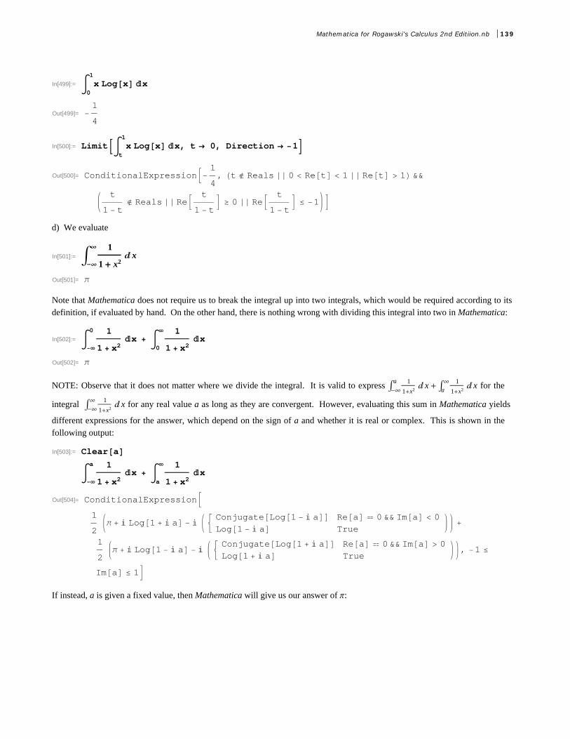
In[499]:= 0

1

x Logx x

Out[499]= 1

4

In[500]:= Limitt

1

x Logx x, t 0, Direction 1

Out[500]= ConditionalExpression 14, t Reals 0 Ret 1 Ret 1 &&

t

1 t Reals Re t

1 t 0 Re t

1 t 1

d) We evaluate

In[501]:= -•

• 1

1 + x2‚ x

Out[501]=

Note that Mathematica does not require us to break the integral up into two integrals, which would be required according to itsdefinition, if evaluated by hand. On the other hand, there is nothing wrong with dividing this integral into two in Mathematica:

In[502]:=

0 1

1 x2x

0

1

1 x2x

Out[502]=

NOTE: Observe that it does not matter where we divide the integral. It is valid to express -¶a 1

1+x2„ x + a

¶ 1

1+x2„ x for the

integral -¶¶ 1

1+x2„ x for any real value a as long as they are convergent. However, evaluating this sum in Mathematica yields

different expressions for the answer, which depend on the sign of a and whether it is real or complex. This is shown in thefollowing output:

In[503]:= Cleara

a 1

1 x2x

a

1

1 x2x

Out[504]= ConditionalExpression1

2 Log1 a ¶ ConjugateLog1 a Rea 0 && Ima 0

Log1 a True

1

2 Log1 a ¶ ConjugateLog1 a Rea 0 && Ima 0

Log1 a True, 1

Ima 1

If instead, a is given a fixed value, then Mathematica will give us our answer of p:


In[505]:= a 1

a 1

1 x2x

a

1

1 x2x

Out[505]= 1

Out[506]=

ü Exercises

In Excercises 1 through 8, evaluate the given improper integrals:

1. -¶4 ‰.01 t „ t 2. -3¶ 1

x+432 „ x 3. -24 1

x+213 „ x 4. -¶¶ x ‰-x2„ x

5. 03 1

x-1„ x 6. -¶¶ 1

ex+e-x „ x 7. 1¶ 1

x.999„ x 8. 1

¶ 1

x1.003„ x

11. Find the volume of the solid obtained by rotating the region below the graph of y = ‰-x about the x-axis for 0 § x <¶.

12. Determine how large the number b has to be in order that b¶ 1

x2+1„ x < .0001.

13. Evaluate the improper integral -11 1

x3

„ x.

14. Determine how large the number b should be so that b

¶ 1

x2+1„ x < .0001.

15. Consider the function defined by

Gx = 0¶

tx-1 e-t „ t

a) Evaluate Gn for n = 0, 2, , 3, 4, ...., 10. Make a conjecture about these values. Verify your conjecture.b) Evaluate G2 n - 1 2, for n = 1, 2, 3, ... 10. Make a conjecture about these values. Verify your conjecture.c) Plot the graph of Gx on the interval 0, 5.NOTE: The function G is called the gamma function and is denoted by Gx. In Mathematica it is denoted by Gamma[x]. Thegamma function was first introduced by Euler as a generalization of the factorial function.

ü 7.4 Hyperbolic and Inverse Hyperbolic Functions


ü 7.4.1. Hyperbolic Functions

The hyperbolic functions are defined in terms of the exponential functions. They have a direct connection to engineeringmathematics, including bridge construction. For example, cables from suspension bridges typically form a curve called acatenary (derived from the Latin word catena, which means chain) that is described by these functions.

The six hyperbolic functions are denoted and defined as follows:

sinh x = ex- e-x

2, cosh x = ex+ e-x

2, tanh x = ex- e-x

ex+ e-x

coth x = ex+ e-x

ex- e-x , sech x = 2

ex+ e-x , csch x = 2

ex- e-x


The reason these functions are called hyperbolic functions is due to their connection with the equilateral hyperbola x2 - y2 = 1.

Here, one defines x = cosh t and y = sinh t. Hence, one obtains the basic hyperbolic identity cosh2 t - sinh2 t = 1, much the same

manner as the corresponding trigonometric identity cos2 t + sin2 t = 1, when one considers the unit circle x2 + y2 = 1 withx = cos t and y = sin t.

In Mathematica, we use the same notation with the obvious convention that the first letter of each function is capitalized and

square brackets must be used in place of parentheses. Thus, sinh x will be entered as Sinh[x].

Example 7.9. Consider the hyperbolic sine function f x = sinh x.a) Plot the graph of f . b) From the graphs deduce the domain and range of the function. c) Is f bounded? d) Does f attain an absolute minimum? Maximum?e) Repeat a) through d) for the hyperbolic function gx = cosh x f) Repeat a) through d) for the hyperbolic function hx = tanh x.

Solution: We begin by defining f in Mathematica:

In[507]:= Clearf, xfx_ Sinhx

Out[508]= Sinhxa) We next plot its graph on the interval -3, 3.In[509]:= Plotfx, x, 3, 3

Out[509]=-3 -2 -1 1 2 3

-10

-5

5

10

b) The preceding graph indicates that the domain and range of sinh x is -¶, ¶. To convince yourself, you should plot the graphover wider intervals. We should also expect this from the definition of sinh x itself. Can you explain why?

c) The function sinh x is not bounded. The graph earlier should not be used as a proof of this. However, we can evaluate its limitat -¶ and ¶ to see that this is indeed true.

In[510]:= Limitfx, x Limitfx, x

Out[510]=

Out[511]=

d) The limits just computed show that sinh x has no absolute maximum or minimum since it is unbounded.

e) Next, we consider the hyperbolic cosine function denoted by cosh x.


In[512]:= Clearg, xgx_ Coshx

Out[513]= CoshxIn[514]:= Plotgx, x, 3, 3

Out[514]=

-3 -2 -1 1 2 3

4

6

8

10

The preceding graph indicates that the domain of cosh x is -¶, ¶. The range appears to be 1, ¶. Can you prove this?

The hyperbolic cosine function, cosh x, is not bounded from above. This can be seen from the following limits:

In[515]:= LimitCoshx, x LimitCoshx, x

Out[515]=

Out[516]=

Again, since cosh x is not bounded from above, it follows that cosh x has no absolute maximum. As we have observed in part b)of this example, cosh x has absolute minimum value 1, attained at x = 0.

f) Finally, we consider the hyperbolic tangent function, tanh x:

In[517]:= Clearh, xhx_ Tanhx

Out[518]= TanhxIn[519]:= Plothx, x, 3, 3

Out[519]=-3 -2 -1 1 2 3

-1.0

-0.5

0.5

1.0


Again, the preceding graph indicates that the domain of tanh x is -¶, ¶. The range appears to be -1, 1. This can be seenfrom the following limits:

In[520]:= LimitTanhx, x LimitTanhx, x

Out[520]= 1

Out[521]= 1

The graph of tanh x also indicates that it is strictly increasing on its domain. This can be proven by showing that its derivative,which we will calculate later, is strictly positive. It is clear that tanh x has no absolute extrema.

NOTE: The reader will notice some similarities between the hyperbolic functions and the associated trigonometric functions.Moreover, if one studies the theory of functions of a complex variable, the relationship between these classes of transcendentalfunctions becomes even more transparent; for numerous identities exist between the classes of functions.

ü 7.4.2 Identities Involving Hyperbolic Functions

It is immediate that the ratio and reciprocal identities for the hyperbolic functions coincide with their trigonometric counterparts.In fact, for each trigonometric identity, there is a corresponding (not necessarily the same) hyperbolic identity. Following aresome examples.

Example 7.10. Show that the following identities hold true.

a) 1 - tanh2 x = sech2 x b) coshx + y = cosh x cosh y + sinh x sinh y

Solution:

a) We use the definitions for tanh x and sech x to express each side of the identity in terms of exponentials:

In[522]:= Simplify1 Tanhx2 . Tanhx E^x E^x E^x E^x

Out[522]=4 2 x

1 2 x2

In[523]:= SimplifySechx2 . Sechx 2 E^x E^x

Out[523]=4

x x2

We leave it for the reader to verify that both of these outputs agree, that is, 4 e2 x

1+e2 x2 =4

e-x+ex2 (cross-multiply and then simplify).

The identity can also be confirmed in Mathematica by evaluating the difference between its left- and right-hand sides, whichshould equal zero:

In[524]:= Simplify1 Tanhx2 Sechx2Out[524]= 0

NOTE: We can also confirm the identity graphically by plotting the graphs of each side of the identity, which should coincide.


In[525]:= Plot1 Tanhx^2, Sechx^2, x, 2, 2

Out[525]=

-2 -1 1 2

0.2

0.4

0.6

0.8

1.0

b) We again evaluate the difference between the left- and right-hand sides of the identity:

In[526]:= SimplifyCoshx y Coshx Coshy Sinhx SinhyOut[526]= 0

ü 7.4.3 Derivatives of Hyperbolic Functions

We next contrast the formulas for the derivatives of the trigonometric functions versus the formulas for the derivatives of thecompanion hyperbolic functions.

Example 7.11. Compare the derivatives of the given pair of functions.a) sinh x and sin x b) cosh x and cos x c) tanh x and tan x

Solution: We use the derivative command, D, to evaluate derivatives of each pair.

a)

In[527]:= DSinhx, xDSinx, x

Out[527]= CoshxOut[528]= Cosxb)

In[529]:= DCoshx, xDCosx, x

Out[529]= SinhxOut[530]= Sinxb)

In[531]:= DTanhx, xDTanx, x

Out[531]= Sechx2Out[532]= Secx2


It is clear that derivatives of hyperbolic and trigonometric functions are quite similar.

ü 7.4.4 Inverse Hyperbolic Functions

In light of the fact that hyperbolic functions are defined in terms of the exponential functions, it is readily apparent that theinverse hyperbolic functions are defined in terms of the natural logarithmic function. The inverses of the hyperbolic functions

have notation similar to those of inverse trigonometric functions. Thus, the inverse of sinh x is denoted by arcsinh x or sinh-1 x.

In Mathematica, the notation is sinh-1 x is ArcSinh[x].

Example 7.12. Plot the graphs of sinh-1 x and sinh x on the same axis.

Solution: Recall that the graph of a function and the graph of its inverse are reflections of each other across the line y = x. This

is confirmed by the following plot of sinh-1 x (in blue) and sin x (in red).

In[533]:= PlotSinhx, x, ArcSinhx, x, 3, 3,PlotStyle Blue, Green, Red, AspectRatio Automatic, PlotRange 3, 3

Out[533]=-3 -2 -1 1 2 3

-3

-2

-1

1

2

3

Example 7.13. Show that tanh-1 x = 1

2ln 1+x

1-x for -1 < x < 1.

Solution: We plot the graphs of y = tanh-1 x and y = 1

2ln 1+x

1-x on the same axes. Note that Mathematica's notation of tanh-1 x is

ArcTanh [x] and ln y is entered as Log[y]:


In[534]:= PlotArcTanhx, 1

2Log 1 x

1 x, x, 2, 2

Out[534]=-2 -1 1 2

-3

-2

-1

1

2

3

The fact that there is only one graph indicates that the functions are the same. We prove this by letting y = tanh-1 x and solving

for y as follows. From y = tanh-1 x we get x = tanh y = ey-e-y

ey+e-y . Now solving this last equation for y in Mathematica yields:

In[535]:= Solvex E^y E^y E^y E^y, ySolve::ifun : Inverse functions are being used by Solve, so

some solutions may not be found; use Reduce for complete solution information. à

Out[535]= y Log 1 x

1 x, y Log 1 x

1 x

The first solution in the preceding output is imaginary, which we ignore, and consider only the second solution. Hence,

tanh-1 x = y = ln -1-x

-1+x= ln 1+x

1-x= 1

2ln 1+x

1-x .

NOTE: The message in the previous output refers to the fact that when solving equations involving inverse functions, not allsolutions are necessarily found by Mathematica since there may be infinitely many of them or they depend on the domain ofdefinition. For example, the equation sin x = 1 has infinitely many solutions, in particular all values of the form x = p 2 + 2 p n,where n is any integer. On the other hand, solving this equation in Mathematica yields only the solution in its principal domain,that is, x = p 2:

In[536]:= SolveSinx 1, xSolve::ifun : Inverse functions are being used by Solve, so


Out[536]= x

2

ü Exercises

In Exercises 1 through 5, verify the given hyperbolic identities using the Simplify command. Also state the correspondingtrigonometric identity.

1. sinhx + y = sinh x cosh y + cosh x sinh y 2. cosh 2 x = cosh2 x + sinh2 x 3. tanh 2 x = 2 tanh x

1+tanh2 x

4. coshx + y = cosh x cosh y + sonh x sinh y 5. tanhx + y = tanh x+tanh y

1+tanh x tanh y


6. Determine the first few positive integral powers of cosh x + sinh x. Can you form a general conjecture for the nth case,namely cosh x + sinh xn, where n is any natural number? Then justify your conclusion via mathematical induction.

In Exercises 7 through 12, determine the derivatives of thegiven functions and simplify your answers where possible. Compareyour solution via paper and pencil methods with the one generated by Mathematica.

7. f x = tanh 1 + x2 8. f x = x sinh x - cosh x 9. f x = 1+tanh x

1- tanh x

10. f x = x2 sinh-12 x 11. f x = x tanh-1 x + ln 1 - x2 12. f x = x coth x - sech x

13. The Gateway Arch in St. Louis was designed by Eero Saarinen and was constructed using the equation

y = 211.49 - 20.96 cosh 0.03291765 x for the central curve of the arch, where x and y are measured in meters and x § 91.20.

a) Plot the graph of the central curve.b) What is the height of the arch at its center?c) At what points is the arch 100 meters in height?d) What is the slope of the arch at the points in part (c)?

14. A flexible cable always hangs in the shape of a catenary y = c + a cosh x a, where c and a are constants and a > 0. Plotseveral members of the family of functions y = a cosh x a for various values of a. How does the graph change as a varies?

In Exercises 15 through 17, evaluate each of the given integrals:

15. sinh x coshn x „ x 16. cosh x

cosh2 x-1„ x 17. sech2 x

2+tanh x„ x

18. Let t = ln 1+ 5

2 and define

f n = 2

5cosht n, if n is odd

2

5sinh t n, if n is even

Evaluate f n for n = 1, 2, 3, ..., 20. Do these values seem familiar? If not, we highly recommend the interesting article byThomas Osler, Vieta-like products of nested radicals with Fibonacci and Lucas numbers, to appear in the journal FibonacciQuarterly.


Chapter 8 Further Applications of Integration

ü 8.1 Arc Length and Surface Area


ü 8.1.1 Arc Length

The integrals for calculating arc length and surface area are generally difficult to do by hand. Thus, Mathematica is the appropri-ate tool for evaluating these integrals.

If y is a function of x, that is, y = f x, and f ' x exists and is continuous on a, b, then the arc length of the graph of f x overthe interval a, b is

L = a

b1 + f ' x2 „ x

If x is a function of y, that is, x = g y, and g ' y exists and is continuous on c, d, then the arc length of the graph of g y overthe interval c, d is

L = cd

f ' y2 + 1 „ y

Example 8.1. Estimate the arc length of y = 1

x over the interval 1, 2.

Solution: Finding the arc length of this simple rational function by hand is virtually impossible. This is because f ' x = - 1

x2 and

thus the arc length integral is L = 12

1 + 1

x4„ x, which cannot be evaluated in terms of elementary functions, as the following

answer illustrates.

In[537]:= 1

2

1 1

x4x

Out[537]=

2 Gamma 74

3 Gamma 54

1

2Hypergeometric2F1 1

2,

1

4,3

4, 16

However, there are numerical techniques that we can use. For example, the Mathematica command NIntegrate uses sophisti-cated algorithms to gives us a good estimate for this definite integral:

In[538]:= NIntegrate 1 1

x4, x, 1, 2

Out[538]= 1.13209

A more elementary method of estimating this arc length is Simpson's Rule as shown in Section 7.1 of this text.


In[539]:= Clearf, a, b, nSIMPa_, b_, n_, f_ :

1 3 Sumfa 2 i 2 b a n 4 fa 2 i 1 b a n

fa 2 i b a n, i, 1, n 2 b a n

In[541]:= fx_ : 1 1

x4

TableFormTablen, NSIMP1, 2, n, f, n, 10, 100, 10,TableHeadings , "n", "Sn"


n Sn

10 1.132120 1.1320930 1.1320940 1.1320950 1.1320960 1.1320970 1.1320980 1.1320990 1.13209100 1.13209

Thus, we see that Simpson's Rule gives us as accurate an estimate of the arc length, as does the NIntegrate command for n assmall as 20.

Example 8.2. Consider the the ellipse whose equation is given by

x2

a2+

y2

b2= 1

Assume that a > b. Find the arc length of the upper half of the ellipse.

Solution: To plot the ellipse for various values of a and b, we define a plotting command plot[a,b] as follows.

In[543]:= Cleara, b, x, y, eq, plot

eqx_, y_, a_, b_ :x2

a2y2

b2 1

plota_, b_ : ContourPloteqx, y, a, b 0, x, a, a, y, b, b,AspectRatio Automatic, Axes True, Frame False

Here is a plot of the ellipse for a = 2 and b = 3.


In[546]:= plot2, 3

Out[546]=-2 -1 1 2

-3

-2

-1

1

2

3

On the upper half of the ellipse, we have y ¥ 0. Thus, we can solve for y and and take the positive solution. We will denote thispositive solution as a function of x, a, and b.

In[547]:= sol Solvex2

a2y2

b2 1, y;

fx_, a_, b_ sol2, 1, 2

Out[548]=b a2 x2

a

Clearly, the domain of f is -a, a. The natural thing to do would be to evaluate the integral -a

a1 + f ' x2 „ x. Try this

yourself, but be prepared to wait awhile. Moreover, Mathematica will give the following output:

IfIma 0 && a Im 1

a2 b2 1

1 a Im 1

a2 b2 0 a Im 1

a2 b2 0 a Re 1

a2 b2 0 ,


2 a32 b2 EllipticE1 b2

a2 Signa

a b2, Integrate 1

b2 x2

a4 a2 x2, x, a, a,

Assumptions Reb 0 && Rea 0 && Ima 0 && Imb 0 Ima 0 Ima 0

To understand this output, let us make a change of variable x = a sin t. Then the integral becomes (verify this)

-a

a1 + f ' x2 „ x = a -p2p2

1 + b2 sin2 t

a2 cos2 tcos t d t

The latter integral can be expressed as

2 a 0

p21 + b2 sin2 t

a2 cos2 tcos t d t = 2 a 0

p2cos2 t + b2 a2 sin2 t d t = 2 a 0

p21 - c2 sin2 t d t ,

where c = 1 - b a2 and we have used the identity cos2 t = 1 - sin2 t.

To simplify our notation, let us define the integrand in the preceding far left integral as

In[549]:= gt_, a_, b_ 1 1 b a2 Sint2

Out[549]= 1 1 b2

a2Sint2

Here are some values of the arc length of the upper half of the ellipse.

In[550]:= TableFormTable2 a 0

2gt, a, b t, a, 1, 3, b, 1, 3,

TableHeadings "a1", "a2", "a3", "b1", "b2", "b3" Out[550]//TableForm=

b1 b2 b3a1 2 EllipticE3 2 EllipticE8a2 4 EllipticE 3

4 2 4 EllipticE 5

4

a3 6 EllipticE 89 6 EllipticE 5

9 3

Observe that we obtain exact values for the arc length when a = b. Can you explain why?

The approximate values of the numbers appearing in the preceding table are as follows:

In[551]:= TableFormNTable2 a 0

2gt, a, b t, a, 1, 3, b, 1, 3, 10,

TableHeadings "a1", "a2", "a3", "b1", "b2", "b3" Out[551]//TableForm=

b1 b2 b3a1 3.141592654 4.844224110 6.682446610a2 4.844224110 6.283185307 7.932719795a3 6.682446610 7.932719795 9.424777961


NOTE: The integral 1 - c2 sin2 t „ t is known as an elliptic integral. It is very useful in mathematics and has many applica-

tions. In Mathematica, it is denoted by Elliptic[t,c^2]. The command Elliptic[x,m] gives 0

x1 -m sin2 t dt, while Elliptic[m]

gives 0

p21 -m sin2 t dt.

ü 8.1.2 Surface Area

If f ' x exists and is continuous on a, b, then the surface area of revolution obtained by rotating the graph of f x about the x-axis for a § x § b is

S = 2 p a

bf x 1 + f ' x2 „ x

Similarly, if x = gy and g ' y exists and is continuous on c, d, then the surface area of revolution obtained by rotating g yabout the y-axis for c § y § d is

S = 2 p cdgy g ' y2 + 1 „ y

Again, evaluating these complicated integrals is what Mathematica does best, as the following examples illustrate.

Example 8.3. Determine the surface area of revolution obtained by rotating the region under y = ‰-x along the interval 0, 2about the x-axis.

Solution: We calculate

In[552]:= Clearf, xfx_ : x

S 2 0

2

fx 1 f'x2 x

Out[554]=1

2 4 2 2

2

1 4

2

4 1 4 Log3 2 2 Log2 4 2 1 4

In[555]:= NOut[555]= 6.35887

Here is the corresponding surface of revolution (rotated 90 ° about the y-axis):


In[556]:= RevolutionPlot3DEx, x, 0, 2

Out[556]=

NOTE: Observe that in this case Mathematica was able to find an anti-derivative of the integrand. However, not all integrals ofthis form can be evaluated analytically as the next example illustrates.

Example 8.4. Determine the surface area of revolution obtained by rotating the region under y = tan x along the interval 0, p

4

about the x-axis.

Solution: As in the previous example, we evaluate

In[557]:= Clearf, xfx_ : TanxNIntegrate2 fx 1 f'x2 , x, 0, Pi 4

Out[559]= 3.83908

To appreciate the complexity of the integral and understand why we used the command NIntegrate, we advise the reader to

define the anti-derivative F[t] below and evaluate F[p/4] (be prepared to wait awhile).

In[560]:= Ft_ : Integratefx 1 f'x2 , x, 0, tHere is the corresponding surface of revolution:


In[561]:= RevolutionPlot3DTanx, x, 0, Pi 4

Out[561]=

ü Exercises

In Exercises 1 and 2, calculate the arc length of the given function over the given interval:

1. y = x4, over 1, 2 2. y = sin x, over 0, p

2

3. Calculate the arc length of the astroid x23 + y23 = 1. Below is a plot of its graph. Hint: By symmetry it suffices to calculateonly the portion in the first quadrant.

In[562]:= ContourPlotx^2^1 3 y^2^1 3 1, x, 1, 1, y, 1, 1

Out[562]=

-1.0 -0.5 0.0 0.5 1.0

-1.0

-0.5

0.0

0.5

1.0

4. Show that the circumference of the unit circle is 2p by calculating its arc length. Use the fact that the equation of the unitcircle is given by x2 + y2 = 1.


In Exercises 5 through 7, compute the surface area of the given functions rotated about the x-axis over the given intervals:

5. y = x3 + 1

x, over 1, 4 6. y = 4 - x2323

over 0, 8 7. y = cos x, over 0, p 8. Show that the surface area of the unit sphere is 4p by rotating the top half of the unit circle x2 + y2 = 1 about the x-axis.

ü 8.2 Center of Mass


A lamina is a thin plate whose mass is distributed throughout a region in the plane. Suppose a lamina has a constant density r andthat the lamina occupies a region in the plane under the graph of a continuous function f over the interval a, b, where f x ¥ 0for all x.

The mass of the lamina is given by

M = r ab

f x „ x

Then the moments of the lamina with respect to x-axis and y-axis are denoted by Mx and My and are defined by

Mx =1

2r a

b f x2 „ x

My = r a

bx f x „ x

The center of mass (also called the centroid) of the lamina is defined to be x, y, where

x =My

M and y = Mx

M

NOTE: If the lamina described above as a density r that continuously depends on x, that is, if r = rx for x in the interval a, b,then the moments, the total mass, and the center of mass are given by

M = a

brx f x „ x

Mx =1

2 a

brx f x2 „ x

My = a

bx rx f x „ x

x =My

M and y = Mx

M

Example 8.5. Suppose a lamina lies underneath the graph of y = 16 - x2 and over the interval -4, 4.

a) Assume the density of the lamina is r = 3. Find the mass, moments, and the center of mass of the lamina. b) Assume the density of the lamina is r = x

2+ 2. Find the mass, moments, and the center of mass of the lamina.

Solution:

a) We use the above formulas with r = 3:


In[563]:= fx_ 16 x2

Out[563]= 16 x2

The mass is given by

In[564]:= M 3 4

4

fx xOut[564]= 256

The moment with respect to the x-axis is

In[565]:= Mx 3 2 4

4

fx2 x

Out[565]=8192

5

The moment with respect to the y-axis is

In[566]:= My 3 4

4

x fx xOut[566]= 0

The coordinates for the center of mass are

In[567]:= xbar My Mybar Mx M

Out[567]= 0

Out[568]=32

5

Observe that the region of the lamina is symmetric with respect to the y-axis. Hence, the fact that x = 0 is also clear from the factthat the density is a constant.

Below is the plot of the lamina and its center of mass:

In[569]:= plot1 Plotfx, x, 4, 4 , Filling Axis;plot2 ListPlotxbar, ybar, PlotStyle PointSize0.02, Red;Showplot1, plot2

Out[571]=


b) Here, r = x + 4. With the above notation we have

In[572]:= fx_ 16 x2

x_ x

2 2

Out[572]= 16 x2

Out[573]= 2 x

2

The mass is

In[574]:= Mv 4

4

x fx x

Out[574]=512

3

The moment with respect to the x-axis is

In[575]:= Mxv 1 2 4

4

x fx2 x

Out[575]=16384

15

The moment with respect to the y-axis is

In[576]:= Myv 4

4

x x fx x

Out[576]=2048

15


In[577]:= xbarv Myv Mybarv Mxv M

Out[577]=8

15

Out[578]=64

15

Here is a plot of the lamina showing the center of masses with the uniform density of r = 3 and variable density of r = x

2+ 2

represented by the red and green dots, respectively.


In[579]:= plot3 ListPlot xbarv, ybarv, PlotStyle Green, PointSize.02;Showplot1, plot2, plot3

Out[580]=

NOTE: Observe that the center of mass with variable density (green dot) is shifted to the right, as expected, since the density ismore weighted to the right.

Example 8.6. Suppose a lamina covers the top half of the ellipse

x2

a2+

y2

b2= 1

a) Assume the density of the lamina is r = 1. Find the mass, moments and the center of mass of the lamina. b) Assume the density of the lamina is r = e-x. Find the mass, moments and the center of mass of the lamina.

Solution: To distinguish between the uniform and variable density cases in parts a) and b), respectively, we attach the letter u

and v to the notation in this solution. Thus, Mu will be the mass corresponding to the uniform density while Mv is the masscorresponding the variable density.

a) We solve the equation of the ellipse for y:

In[581]:= Cleara, b, x, y

sol Solvex2

a2y2

b2 1, y

Out[582]= y b a2 x2

a, y

b a2 x2

a

In the top half of the ellipse , we have y ¥ 0. Thus, we take the second solution, simplify, and define it as a function of x, a, and b

In[583]:= fax_, a_, b_ : b 1 x2

a2

Let the mass, the moment with respect to the x-axis, the moment with respect to the y - axis , and the center of mass be denotedby M a, b, Mxa, b, Mya, b, and xa, b, ya, b), respectively. We now compute these quantities assuming r = 1.


In[584]:= Cleara, b, Mua, Mxua, Myua, xbaru, ybaruMuaa_, b_

a

a

fax, a, b x

Mxuaa_, b_ 1 2 a

a

fax, a, b2 x

Myuaa_, b_ a

a

x fax, a, b x

Out[585]=a b

2

Out[586]=2 a b2

3

Out[587]= 0

In[588]:= xbaruaa_, b_ Myuaa, bMuaa, b

ybaruaa_, b_ Mxuaa, bMuaa, b

Out[588]= 0

Out[589]=4 b

3

That x = 0 is also clear from the fact that the density is a constant and the upper half of the ellipse is symmetric with respect tothe y -axis.

The mass of the lamina, the moments of the lamina with respect to the x- and y-axis for various values of a and b are as follows:


In[590]:= umassa TableFormTableMuaa, b, a, 1, 3, b, 1, 3,TableHeadings "a1", "a2", "a3", "b1", "b2", "b3";

uxmomenta TableForm TableMxuaa, b , a, 1, 3, b, 1, 3 ,TableHeadings "a1", "a2", "a3", "b1", "b2", "b3";

uymomenta TableForm TableMyuaa, b , a, 1, 3, b, 1, 3 ,TableHeadings "a1", "a2", "a3", "b1", "b2", "b3";

TableFormumassa, uxmomenta, uymomenta,TableHeadings "Mass", "xmoment", "ymoment",


Mass

b1 b2 b3

a1

2 3

2

a2 2 3

a3 3 2

3 9 2

xmoment

b1 b2 b3

a1 23

83

6

a2 43

163

12

a3 2 8 18

ymoment

b1 b2 b3a1 0 0 0a2 0 0 0a3 0 0 0

The corresponding y-coordinate of the center of mass in each case is (recall that x = 0 for all cases)

In[594]:= centermassua Table Mxuaa, bMuaa, b , a, 1, 3, b, 1, 3;

TableFormcentermassua,TableHeadings "a1", "a2", "a3", "b1", "b2", "b3"


b1 b2 b3

a1 43

83

4

a2 43

83

4

a3 43

83

4

The following animation shows how the center of mass changes as a and b varies.

In[596]:= plot4aa_, b_ :

Plotfx, a, b, x, a, a, PlotRange 5, 5, 15, 15, Filling Axis;plot5aa_, b_ : ListPlot Myuaa, b

Muaa, b ,Mxuaa, bMuaa, b ,

PlotStyle Red, PointSize0.02plotuaa_, b_ : Showplot4aa, b, plot5aa, b

Important Note:: If you are reading the printed version of this publication, then you will not be able to view any of the anima-


ted as a Mathematica Notebook, then evaluate each Animate command to view the corresponding animation. Just click on the


arrow button to start the animation. To control the animation just click at various points on the sliding bar or else manually dragthe bar.

In[599]:= Animateplotuaa, b, a, 1, 8, b, 1, 10

Out[599]=

a

b

-4 -2 2 4

-15

-10

-5

5

10

15

b) Here, r = e-x. With the above notations modified to reflect variable density, we have

In[600]:= Cleara, b, Mv, Mxv, Myv, xbarv, ybarvx_ Ex

Mvba_, b_ a

a

x fax, a, b x

Mxvba_, b_ 1 2 a

a

x fax, a, b2 x

Myvba_, b_ a

a

x x fax, a, b xOut[601]= x

Out[602]= ConditionalExpressionb BesselI1, a, a 0

Out[603]=2 b2 a Cosha Sinha

a2

Out[604]= ConditionalExpressiona b BesselI2, a, a 0


In[605]:= xbarvba_, b_ Myvba, bMvba, b

ybarva_, b_ Mxvba, bMvba, b

Out[605]= ConditionalExpression a BesselI2, aBesselI1, a , a 0

Out[606]= ConditionalExpression2 b a Cosha Sinhaa2 BesselI1, a , a 0

Observe that the formulas for the mass and moments of the lamina are no longer elementary. Here is a table of numerical valuesfor these quantities assuming various choices for a and b:

In[607]:= umassb TableFormTableMvba, b, a, 1, 3, b, 1, 3,TableHeadings "a1", "a2", "a3", "b1", "b2", "b3";

uxmomentb TableForm TableMxvba, b , a, 1, 3, b, 1, 3 ,TableHeadings "a1", "a2", "a3", "b1", "b2", "b3";

uymomentb TableForm TableMyvba, b , a, 1, 3, b, 1, 3 ,

TableHeadings "a1", "a2", "a3", "b1", "b2", "b3";TableFormNumassb, uxmomentb, uymomentb,TableHeadings "Mass", "xmoment", "ymoment",


Mass

b1 b2 b3a1 1.7755 3.551 5.3265a2 4.99713 9.99427 14.9914a3 12.4199 24.8398 37.2596

xmoment

b1 b2 b3a1 0.735759 2.94304 6.62183a2 1.94877 7.79506 17.5389a3 4.48558 17.9423 40.3702

ymoment

b1 b2 b3a1 0.426464 0.852928 1.27939a2 4.32879 8.65758 12.9864a3 21.1606 42.3213 63.4819


In[611]:= centermassvb NTable Myvba, bMvba, b ,

Mxvba, bMvba, b , a, 1, 3, b, 1, 3

Out[611]= 0.240194, 0.414395, 0.240194, 0.828791, 0.240194, 1.24319,0.866255, 0.389977, 0.866255, 0.779953, 0.866255, 1.16993,1.70377, 0.361161, 1.70377, 0.722323, 1.70377, 1.08348

Here is a plot showing the two centers of mass with for uniform and variable density.


In[612]:=

plot4ba_, b_ : Plotfx, a, b, x, a, a,PlotRange 8, 8, 1, 8, AspectRatio Automatic, Filling Axis;

plot5ba_, b_ : ListPlot Myvba, bMvba, b ,

Mxvba, bMvba, b ,

PlotStyle Green, PointSize0.02plotvba_, b_ : Showplot4ba, b, plot5ba, b




In[615]:= Animateplotvba, b, a, 1, 8, b, 1, 8

Out[615]=

a

b

-5 5

2

4

6

8

ü Exercises

1. Suppose a lamina is lying underneath the graph of y = 1 + x2 over the interval 0, 2 .a) Assume the density of the lamina is r = 3. Find the mass, moments, and the center of mass of the lamina. b) Assume the density of the lamina is r = 2 x. Find the mass, moments, and the center of mass of the lamina. c) Plot the lamina and the center of mass on the same axes for both parts a) and b) above.

2. Suppose a lamina of constant density r = 2 is in the shape of the astroid x23 + y23 = 1. Find its mass, moments, and centerof mass. Plot the lamina with its center of mass.


Chapter 9 Introduction to Differential Equations

ü 9.1 Solving Differential Equations


An ordinary differential equation is an equation that involves an unknown function, its derivatives, and an independent variable.Differential equations are useful for modeling many physical phenomena some of which are discussed in the next section.

Given a differential equation, our objective is to find all functions that satisfy it. Mathematica's command for solving a differen-

tial equation is DSolve[eqn,y[x],x] where eqn is the differential equation to be solved and y[x] is the unknown function that

depends on the independent variable x.

If the differential equation has initial conditions, we use braces to group the equation as well as the initial conditions (separated

by commas): DSolve[{eqn,cond1,cond2,...,condn},y[x],x], where cond1, cond2,...,condn are initial conditions.

ü 9.1.1. Separation of Variables

As discussed in your textbook, there is a special class of first-order differential equations that can be solved by hand using themethod of separation of variables. Mathematica can help in applying this method but of course it can solve the differentialequation outright. This makes Mathematica useful for verifying solutions obtained by other methods or for solving more compli-cated differential equations. Since your textbook focuses on solving differential equations by hand, we will primarily discusshow to solve them using Mathematica.

Example 9.1. Solve the given differential equation and plot the graph of the solutions.

a) y ' = 2 4 - y, y0 = 1 b) 1 - x2 y ' = x y c) yd y

d x+ 5 x = 0

Solution:

a) This is an initial value problem. Let us first solve this differential equation by hand using the method of separation of vari-ables:

dy

dx= 2 4 - y ï

dy

y-4= -2 dx

dy

y-4= - 2 dx

log y - 4 = -2 x + Cy - 4 = e-2 x+C = eC e-2 x

y - 4 = ≤eC e-2 x = C e-2 x (≤eC replaced by C)This shows that the general solution is given by

y = C e-2 x + 4

It remains to determine the value of the constant C using the initial condition y0 = 1 (recall from your textbook that each valueof C corresponds to a particular solution):

1 = y0 = C e-2ÿ0 + 4 = C + 4

Thus, C = -3 and the unique solution is

y = -3 e-2 x + 4


Next, let us confirm this solution using Mathematica. Recall that when entering a differential equation in Mathematica, we writeyx instead of y to make explicit the dependence on x.

In[616]:= sola DSolvey'x 2 4 yx, yx, xOut[616]= yx 4 2 x C1This solution agrees with the solution obtained earlier by hand (the arbitrary constant C1 is the same to the constant C). We canvisualize the behavior of the particular solutions by plotting some of their graphs for different values of C1. First, let us definethe general solution to be gx, c, where c = C1 as follows (see Section 1.2.3 to learn how to extract elements from lists):

In[617]:= Clearg, x, cgx_, c_ sola1, 1, 2 . C1 c

Out[618]= 4 c 2 x

We then plot the one-parameter family of solution curves by combining the graphs of gx, c for c = -5, -4, ..., 5.

In[619]:= plotgeneralsolution

PlotTablegx, c, c, 5, 5, x, 2, 2, PlotRange 20, 20, ImageSize 250

Out[619]=-2 -1 1 2

-20

-10

10

20

Can you explain how the graph of gx, c varies as c varies? Which c value corresponds to the top graph?

Next, to find the unique particular solution satisfying the given initial condition y0 = 1, we solve the equation g0, c = 1 for c:

In[620]:= Solveg0, c 1, cOut[620]= c 3Thus, our unique solution is y = -3 e-2 x + 4. This agrees with the solution we obtained earlier by hand. Of course, Mathematicacan solve for the unique solution on its own, bypassing the algebraic steps involved:

In[621]:= sola DSolvey'x 2 4 yx, y0 1, yx, xOut[621]= yx 2 x 3 4 2 xHowever, this unique solution does not appear to be the same as the one we obtained earlier. To remedy this, let us extractsolution from the output and define it as y = f x:In[622]:= fx_ sola1, 1, 2Out[622]= 2 x 3 4 2 xWe then apply the Expand command to simplify f x:


In[623]:= ExpandfxOut[623]= 4 3 2 x

Thus, the unique solution obtained by Mathematica is the same as the one obtained by hand. Here is the plot of the uniquesolution:

In[624]:= plotuniquesolution Plotfx, x, 2, 2,PlotRange 20, 20, PlotStyle Thickness0.01, ImageSize 250

Out[624]=-2 -1 1 2

-20

-10

10

20

Lastly, we combine plots of the general solution and the unique solution to show where the latter (bold graph) is situated in theformer:

In[625]:= Showplotgeneralsolution, plotuniquesolution, ImageSize 250

Out[625]=-2 -1 1 2

-20

-10

10

20

b) From this point on, we shall skip using the method of separation of variables, which we leave for the reader to employ, andproceed directly to solving all differential equations using Mathematica as in part a) above.

In[626]:= solb DSolve 1 x2 y'x x yx, yx, x

Out[626]= yx 1x2 C1

Again, we can visualize the behavior of these particular solutions by plotting graphs of some particular solutions correspondingto different values of C1. As before, we define the general solution to be gx, c, where c = C1. In[627]:= Clearg, x, c

gx_, c_ solb1, 1, 2 . C1 c

Out[628]= c 1x2

We then make a combined plot of the graphs of gx, c for c = -5, -4, ..., 5.


In[629]:= PlotTablegx, c, c, 5, 5, x, 2, 2, ImageSize 250

Out[629]=-2 -1 1 2

-4

-2

2

4

c) We again use Mathematica to directly obtain the solution:

In[630]:= Clearysolde DSolve yx y'x 5 x 0, yx, x

Out[631]= yx 5 x2 2 C1 , yx 5 x2 2 C1

Observe that the two solutions, which we denote by f x, c and gx, c, differ only in sign:

In[632]:= fx_, c_ solde2, 1, 2 . C1 c

gx_, c_ solde1, 1, 2 . C1 c

Out[632]= 2 c 5 x2

Out[633]= 2 c 5 x2

The following two plots show the graphs of f x, c and gx, c corresponding to c = -50, -40, ..., 0, ..., 40, 50.

In[634]:= PlotTablefx, c, c, 50, 50, 10,x, 5, 5, PlotRange 0, 10, ImageSize 250

Out[634]=

-4 -2 0 2 4

2

4

6

8

10


In[635]:= PlotTablegx, c, c, 50, 50, 10,x, 5, 5, PlotRange 10, 0, ImageSize 250

Out[635]=

-4 -2 2 4

-10

-8

-6

-4

-2

Observe that the two solutions y = - 5 x2 + 2 c and y = 5 x2 + 2 c can be represented by a single equation:

y2 - 5 x2 = 2 c

which describes a family of hyperbolas. Here is a contour plot of this equation. Observe that it nothing more than a combinationof the two plots above as to be expected.

In[636]:= ContourPloty2 5 x2, x, 5, 5, y, 10, 10, Frame False,

Axes True, ContourShading False, Contours 10, ImageSize 250

Out[636]=

ü Exercises

In Exercises 1 through 8, solve the given differential equations. If initial conditions are also given, then plot the unique solution.If not, then make a combine plot of several particular solutions by choosing various values of the arbitrary constant. Thendescribe the graphs and explain how they vary as the arbitrary constant varies.

1. 1 + x2 y ' = x2 y; y0 = 2 2. y ' + 3 x4 y2 = 0; y0 = 1

3. y ' + y2 = -1; y0 = -1 4. y ' + 3 y = sin x; y0 = 0


5. y ' = -2 x y (bell-shaped curves) 6. 16 y y ' + 9 x = 07. y ' - y = y2 8. 2 x y y ' - y2 + x2 = 0

9. Consider the differential equation

3 + 2 y y ' = 2 - ex, y0 = a

a) Solve the equation.b) Plot the graphs for values of a = -2, -1, 0, 1, 2.c) Plot the graphs for the values of a = -.5, -.1, .1, .5.NOTE: For parts b) and c), make sure to use a sufficiently large interval for x.

10. Consider the differential equation

y = x y b - y 4 + x, y0 = a

a) Solve the equation.b) Plot the graphs for values of a = -2, -1, 0, 1, 2 and b = -2, -1, 0, 1, 2.c) Plot the graphs for the values of a = -.5, -.1, .1, .5 and b = -.5, -.1, .1, .5d) Show that the limit as xØ ¶ of the solution does not depend on a. Does the limit depend on b? If so, how?

11. Suppose a skydiver falls from rest toward the earth and assume that the air resistance caused by his open parachute is propor-tional to the square of his velocity v with proportionality constant k (we neglect air resistance due to the skydiver himself). Amodel for describing the skydiver's velocity after his parachute opens is then given by the differential equation

v ' = - k

mv2 -

m g

k

where m is the mass of the skydiver and g = 9.8 meters/sec2 is his acceleration due to gravity.

a) Solve the equation assuming an initial velocity v0 = v0.b) Suppose that for a particular skydiver m = 70 kg and k = 30 kg meter. Solve the equation again using these values and plot theparticular solutions for the following values of v0: 0, 2, ..., 10.c) What is the skydiver's limiting (terminal) velocity as tØ¶ for each of the particular solutions in part b)? Does it depend onv0?d) Find a formula for the terminal velocity in terms of m, g, and k.

12. Recall that the first-order linear differential equation y ' + y = 0 has solution y = C e-x. Solve the following higher-ordergeneralizations of this equation:

a) y '' + 2 y ' + y = 0b) y ''' + 3 y '' + 3 y ' + y = 0c) y4 + 4 y ''' + 6 y '' + 4 y ' + y = 0d) Do you recognize the coefficients involved in the differential equations above? What would be the next differential equation(of order 5) that follows this pattern? Solve this differential equation to verify that its solution follows that same pattern exhibitedin parts a) through c).

ü 9.2 Models of the Form y ' = ky - bStudents should read Section 9.2 of Rogawski's Calculus [1] for a detailed discussion of the material presented in thissection.

NOTE: The differential equations we encounter in this section can be solved by the method of separation of variables and isdiscussed in the text. We leave it to the reader to solve the examples in this section by hand to verify the solutions obtained using


Mathematica.

ü 9.2.1. Bacteria Growth

The growth of bacteria in a culture is known to be proportional to the amount of the bacteria present at time t. Suppose the initialamount of the bacteria is y0 and the amount at time t is yt. Then the above physical law is modeled by the differential equation

y ' = k y, y0 = y0

where k is the proportionality (growth) constant. Such a model exhibits exponential growth as can be seen from its solution below:

In[637]:= ClearkDSolvey'x k yx, y0 y0, yx, x

Out[638]= yx k x y0NOTE: Since the bacteria is growing in number, yt is increasing and hence y ' t > 0. Thus, k must be a positive number.

Example 9.2. Suppose the amount of bacteria in a culture was 200 at time t = 0. It was found that there were 450 bacteria after 2minutes.a) Find the amount of the bacteria at any time t.

b) At what time will the number of bacteria exceed 10,000?

Solution:

a) First, note that y0 = 200 and y2 = 450. We solve the differential equation y ' = k y with the former as the initial condition:

In[639]:= Cleary, t, ksolde DSolvey't k yt, y0 200, yt, t

Out[640]= yt 200 k tIn[641]:= ft_ solde1, 1, 2Out[641]= 200 k t

To find the value of k we solve f 2 = 450 for k.

In[642]:= solk Solvef2 450, kSolve::ifun : Inverse functions are being used by Solve, so


Out[642]= k 1

2Log 9

4

In[643]:= NOut[643]= k 0.405465

Thus, the proportionality constant is k = 1

2l n9 4 º 0.405465. Substituting this value into yt, we see that the amount of

bacteria at a given time t is

yt = 200 e0.405465 t

b) To find the amount of time it takes for the bacteria to exceed 10,000, we solve


In[644]:= k solk1, 1, 2Solveft 10000, t

Out[644]=1

2Log 9

4

Solve::ifun : Inverse functions are being used by Solve, sosome solutions may not be found; use Reduce for complete solution information. à

Out[645]= t Log50

Log2 Log3

We can approximate this value for t by

In[646]:= NOut[646]= t 9.64824Thus, it takes about 9.64824 minutes for the bacteria to reach 10,000. To visually see this, we plot the graphs of the solutionyt = 200 e0.405465 t (blue curve) and y = 10 000 (red line) on the same axes.

In[647]:= Plotft, 10000, t, 0, 15, PlotStyle Blue, Red, ImageSize 250

Out[647]=

2 4 6 8 10 12 14

5000

10 000

15 000

20 000

NOTE: The solution yt = 200 e0.405465 t is only approximate since we approximated the growth constant k. By using the exact

value for k = 1

2l n9 4 = l n3 2, we can derive the exact solution:

yt = 200 ek t = 200 e t ln3

2 = 200 e ln 3

2t

= 200 3

2t

This agrees with the answer obtained by Mathematica:

In[648]:= ftOut[648]= 25 23t 3t

ü 9.2.2. Radioactive Decay

The differential equation y ' = k y is also used to model the amount of a radioactive substance whose rate of decay is proportionalto the amount present. However, in this case we note that the proportionality constant k < 0. (Explain this!)

Example 9.3. Carbon dating is a method used to determine the age of a fossil based on the amount of radioactive Carbon-14 in itcompared to the amount normally found in the living environment. Suppose that a bone fossil contains 5% of the amount ofCarbon-14 normally found in living animals. If the half-life of Carbon-14 is 5600 years, estimate the age of the bone.

Solution: Let yt) be the amount of Carbon-14 in the bone and let y0 be the initial amount of Carbon-14. Then the differentialequation we need to solve is


In[649]:= Cleark, y, y0solde DSolvey't k yt, y0 y0 , yt, t

Out[650]= yt k t y0

Thus, the solution to the differential equation is yt = y0 ek t. The half-life of Carbon-14 is 5600 implies that y5600 = 1

2y0. We

solve this equation for k:

In[651]:= yt_ solde1, 1, 2solk Solvey5600

1

2y0, k

Out[651]= k t y0

Solve::ifun : Inverse functions are being used by Solve, so


Out[652]= k Log25600

In[653]:= NOut[653]= k 0.000123776Thus, k = -0.000123776. To find the age of the bone, we solve y t = 0.05 y0 (5% of the initial amount) for t.

In[654]:= k Log25600

;

Solveyt 0.05 y0, tSolve::ifun : Inverse functions are being used by Solve, so


Out[655]= t 24202.8Thus, the bone is about 24,203 years old. Observe that it not necessary to know the original amount y0 of Carbon-14 in the bone.

ü 9.2.3. Annuity

An annuity is an investment in which a principal amount of money is placed in a bank account that earns interest at an annualrate (compounded continuously) and the money is withdrawn at a regular interval. The differential equation that models anannuity is given by the annuity equation (rate of change = growth due to interest - withdrawal rate):

P ' t = r Pt -W = rPt - W

r

where Pt is the balance in the annuity at time t, r is the interest rate, and W is the rate (dollars per year) at which money iswithdrawn continuously.

Example 9.4. Find the general solution of the annuity equation for Pt and then use it to calculate the following:a) Assume r = 6% and W = $ 6000 per year and P0 = $ 50 000. Find Pt and determine if and when the annuity runs out ofmoney.b) Assume r = 6% and W = $ 6000 per year and P0 = $ 100 000. Find Pt and determine if and when the annuity runs out ofmoney.c) Assume r = 6% and W = $ 12 000 per year. If we want the annuity to run out of money after 20 years, how much should be


invested now?

Solution: We solve

In[656]:= DSolveP't r Pt W

r, Pt, t

Out[656]= t W

r r t C1

Thus, the general solution is Pt =W r + c er t.

a) We set r = 0.06, W = 6000, and solve the initial value problem:

In[657]:= Clearr, W, Pr 0.06;W 6000;

solde DSolveP't r Pt W

r, P0 50000, Pt, t

Out[660]= Pt 100000. 50000. 0.06 t We then define Pt to be the solution above and plot it to see when the money will run out.

In[661]:= Pt_ solde1, 1, 2PlotPt, t, 0, 15, ImageSize 250

Out[661]= 100000. 50000. 0.06 t

Out[662]=

2 4 6 8 10 12 14

-20 000

-10 000

10 000

20 000

30 000

40 000

50 000

As the graph indicates, the money runs out after approximately 11.5 years. We can confirm this by solving Pt = 0:

In[663]:= NSolvePt 0, tNSolve::ifun : Inverse functions are being used by NSolve, so


Out[663]= t 11.5525b) We repeat the procedure in part a) with the obvious modifications:


In[664]:= Clearr, W, Pr 0.06;W 6000;

solde DSolveP't r Pt W

r, P0 100000, Pt, t;

Pt_ solde1, 1, 2PlotPt, t, 0, 80, ImageSize 250

Out[668]= 100000.

Out[669]=

20 40 60 80

50 000

100 000

150 000

200 000

Observe that the balance Pt = 100, 000 remains constant (can you explain why?) and thus the account will never run out ofmoney. What happens if we invest $100,001? $99,999?

c) In this case, we have r = 0.06 and W = 10 000 per year. The general solution is then given by

In[670]:= Clearr, W, P, cr 0.06;W 12000;

dsol DSolveP't r Pt W

r, P0 c, Pt, t;

Pt_ dsol1, 1, 2Out[674]= 200000. 200000. 0.06 t 1. c 0.06 t

To determine the principal amount that will make the account run out of money in 20 years, we solve P20 = 0 for c:

In[675]:= NSolveP20 0, cOut[675]= c 139761.Thus, we need to invest $139,761.00 now.

ü 9.2.4. Newton's Law of Cooling

Newton's Law of Cooling states that the rate of change in the temperature of an object is proportional to the difference between itstemperature and that of the surrounding environment (known as the ambient temperature). If A is the ambient temperature andTt is the temperature of the object at time t, then the differential equation that models this law is

T ' t = -kTt - A, T0 = T0

where T0 is the initial temperature of the object and k is a positive proportionality constant.

Example 9.6. The temperature in an oven is 350° F when the oven is turned off. After 15 minutes, the temperature is 250° F.


Assume the temperature in the house is 70° F.

a) Find the temperature of the oven at any time t.

b) At what time will the temperature become 75° F? c) What will the temperature be in the limit as tØ ¶?d) Does your answer in c) conform with your physical intuition?

Solution:

a) The ambient temperature here is room temperature. Hence, A = 70. The initial temperature is T0 = 350. Newton's Law ofCooling then gives the model

T ' t = -kTt - 70, T0 = 350

We solve this equation to get

In[676]:= ClearT, ksol DSolveT't k Tt 70, T0 350, Tt, t

Out[677]= Tt 70 k t 4 k tIn[678]:= Tt_ sol1, 1, 2Out[678]= 70 k t 4 k tThus, the solution is Tt = 70 e-k t4 + ek t or Tt = 70 + 280 e-k t. To find the value of k, we solve T15 = 250 for k:

In[679]:= solk SolveT15 250, kSolve::ifun : Inverse functions are being used by Solve, so


Out[679]= k 1

15Log 14

9

In[680]:= k solk1, 1, 2

Out[680]=1

15Log 14

9

In[681]:= NOut[681]= 0.0294555

Thus, k = ln14915

= 0.0294555. Hence, the temperature of the oven at any time t is given by

Tt = 20 + 280 e-0.0294555 t

b) We solve Tt = 75 for t:

In[682]:= NSolveTt 75, tNSolve::ifun : Inverse functions are being used by NSolve, so


Out[682]= t 136.659Thus, the temperature will be 75° F after about two hours and 17 minutes.


c) We make a plot of the solution:

In[683]:= PlotTt, t, 0, 100, AxesOrigin 0, 0, ImageSize 250

Out[683]=

20 40 60 80 100

50

100

150

200

250

300

350

To find the limiting temperature, we evaluate

In[684]:= LimitTt, t InfinityOut[684]= 70

d) Since heat flows from a region of higher temperature to a region of lower temperature, it is intuitively clear that the oven will

cool down to the room (ambient) temperature. Hence, the limit should be 70° F as expected.

ü Exercises

1. Mass of bacteria in a culture grow at a rate proportional to its size. Suppose the culture contains 200 cells intially and there are800 cells after 3 hours.

a) Find the formula for the number of cells in the culture at time t.b) Find the amount of bacteria after 2 hours.c) At what time will the bacteria exceed 10,000 cells?

2. A mummy excavated from an archaelogical site in Egypt is found to contain 20% of Carbon-14 normally found in livinghumans. Use carbon dating to estimate the age of the mummy.

3. Plutonium-239 is a highly radioactive element generated from waste in nuclear power plants and has a half-life of approxi-mately 24,000 years. How many years would it take for Plutonium-239 to decay to a safe level of 1/1000 its original amount?

4. Solve the following using the annuity differential eqaution discussed in this section.a) Assume r = 6% and W = $500 per year and P0 = $5, 000. Find Pt and determine when the annuity runs out of money.b) Assume r = 6% and W = $500 per year and P0 = $9, 000. Find Pt and determine when the annuity runs out of money.c) Assume r = 6% and W = $20, 000 per year. If we want the annuity to run out after 40 years, how much should we investnow?

5. Suppose a retired worker wants to invest in an annuity that will pay out $10,000 per year.a) Assuming the annuity has an interest rate of 5%, find the minimum principal amount that should be invested so that the annuitynever runs out of money.b) Assuming the principal amount of money invested is $250,000, find the minimum interest rate that the annuity should bear sothat it never runs out of money.

6. A hot metal rod is placed in a water bath whose temperature is 40° F. The rod cools from 300° F to 200° F in 1 minute. Howlong will take the rood to cool down to 150° F? 45° F?


ü 9.3 Numerical Methods Using Slope Fields


ü 9.3.1. Slope Fields

Consider a differential equation in the form

y ' = f x, ySince y ' represents the slope of the line tangent to the graph of the solution y, we can think of f x, y as the slope of the sametangent line at the point x, y, which we indicate by drawing a segment of it at the point of tangency. The set of all such linesegments (normalized to have the same length) is called the slope (or direction) field of the differential equation. Note that theslope field gives a graphical approximation to the solution. It enables us to draw or visualize the graph of the unique solution ofthe equation passing through a given point. We will illustrate this in an upcoming example.

To plot the slope field of the differential equation y ' = f x, y along the intervals a, b and c, d on the x- and y-axis, respec-

tively, we use the command VectorPlot[{1, f[x, y]}, {x, a, b}, {y, c, d}], where slope is represented as a two-dimensional vector1, f x, y with the change in x normalized to equal 1.

NOTE: The command VectorPlot replaces the command VectorFieldPlot, which is obsolete in version 7 of Mathematica.

Example 9.9. Consider the differential equation y ' = x2 - 2 y, y0 = -1.

a) Draw the slope fields for the differential equation.b) Solve the differential equation.c) Plot both the slope field and the solution on the same axes.d) Redo parts b) and c) for the same equation but with initial condition given by ya = b. Choose various values for a and b.

Solution:

a) Here, f x, y = x2 - 2 y. We use the VectorPlot command to plot the corresponding slope field:

In[685]:= fx_, y_ : x2 2 y


In[686]:= plot1 VectorPlot1, fx, y, x, 5, 5, y, 10, 10, Axes True,

Frame False, VectorScale Tiny, Tiny, None, ImageSize 250

Out[686]=-4 -2 2 4

-10

-5

5

10

b) We use the DSolve command to find the exact solution of the differential equation.

In[687]:= Cleary, x, gsol DSolvey'x fx, yx, y0 1, yx, xgx_ sol1, 1, 2

Out[688]= yx 1

42 x 5 2 x 2 2 x x 2 2 x x2

Out[689]=1

42 x 5 2 x 2 2 x x 2 2 x x2

c) We now plot the slope field together with the solution above passing through the point 0, -1:In[690]:= plot2 Plotgx, x, 5, 5, PlotRange 10, 10, ImageSize 250

Out[690]=-4 -2 2 4

-10

-5

5

10


In[691]:= Showplot1, plot2, GraphicsPointSizeLarge, Point0, 1, ImageSize 250

Out[691]=-4 -2 2 4

-10

-5

5

10

d) We can show several graphs of solution curves (called integral curves) together with the corresponding slope field. Here is anexample of how this can be done.

In[692]:= Cleary, x, h, a, bsola DSolvey'x fx, yx, ya b, yx, x;hx_, a_, b_ Simplifysola1, 1, 2

Out[694]=1

42 x 1 2 a 2 a2 4 b 2 a 2 x 1 2 x 2 x2

In[695]:= plot3 PlotEvaluateTablehx, a, b, a, 3, 3, 2, b, 3, 3, 2,x, 5, 5, PlotRange 10, 10;

Showplot1, plot3, ImageSize 250

Out[696]=-4 -2 2 4

-10

-5

5

10


ü 9.3.2. Euler's Method

The simplest numerical method for solving a first order differential equation is Euler's Method. This method approximates thesolution by moving along tangent lines described by the slope field of the differential equation. Here is a brief description.

Let y = fx be the solution of the differential equation

y ' = f x, y, yx0 = y0

Then the equation of the line tangent to the graph of y = jx at x = x0 is given by

y = j ' x0 x - x0 + jx0But when x = x0, we have jt0 = y0 and j ' x0 = f x0, y0. Thus, when x is close to x0, jx can be approximated by

y º f x0, y0 x - x0 + y0

We now choose h > 0 to be a small positive number, called the step size, and define x1 = x0 + h. Then jx1 is approximatelyequal to

y1 = y0 + f x0, y0 x1 - x0or

y1 = y0 + h f x0, y0We repeat the above argument at the point x1, y1 to get an approximation of jx2, where x2 = x1 + h = x0 + 2 h:

y2 = y1 + h f x1, y1Proceeding in this manner, we obtain Euler's Method:

yn+1 = yn + h f xn, yn for n = 0, 1, 2, 3, ....

where jxn º yn.

If the approximated solution is calculated over an interval a, b and the step size h is specified, then the number of iterations (orsteps) required is given by m = b - a h, where x0 = a and xn = x0 + n h.

Here is a Mathematica program called Euler for evaluating Euler's Method in m steps (the option SetPrecision sets the precisionof our calculations to 10 digits).

In[697]:= Clearf, x, y, x0, y0, h, mEulerf_, h_, m_ : Modulen,

Doyn 1 SetPrecisionNyn h fxn, yn, 10;xn 1 xn h,n, 0, m

Example 9.7. Use the Euler program to construct a table of solution values for the differential equation y ' = x2 + 2 y, y0 = 1with a step size of h = 0.1 and for m = 10 steps.

Solution: Here f x, y = x2 + 2 y, x0 = 0, y0 = 1.


In[699]:= fx_, y_ : x2 2 y

m 10;x0 0;y0 1;h 0.1;

x0 x0;y0 y0;Eulerf, h, mTableFormTablen, xn, yn, n, 1, m,TableHeadings , "n ", "xn ", "yn"


n xn yn

1 0.1 1.2000000002 0.2 1.4410000003 0.3 1.7332000004 0.4 2.0888400005 0.5 2.5226080006 0.6 3.0521296007 0.7 3.6985555208 0.8 4.4872666249 0.9 5.44871994910 1. 6.619463939

To see how accurate the above approximation is, we solve the differential equation for the exact solution and plot both theapproximate and exact solutions on the same axes.

In[708]:= Clearz, t, exactexact DSolvez't ft, zt, zx0 y0, zt, t;zt_ zt . exact1

Out[710]=1

41 5 2 t 2 t 2 t2

In[711]:= Clearplot1, plot2plot1 Plotzt, t, 0, 1 ;plot2 ListPlotTablexn, yn, n, 0, m, PlotStyle PointSize0.01 ;Showplot1, plot2, ImageSize 250

Out[714]=

0.2 0.4 0.6 0.8 1.0

2

3

4

5

6

7

8

Observe that the approximations become less accurate as we move away from the initial point 0, 1. This is typical of numericalmethods such as Euler's Method. However, we can increase the accuracy of our approximation by decreasing the step size. For


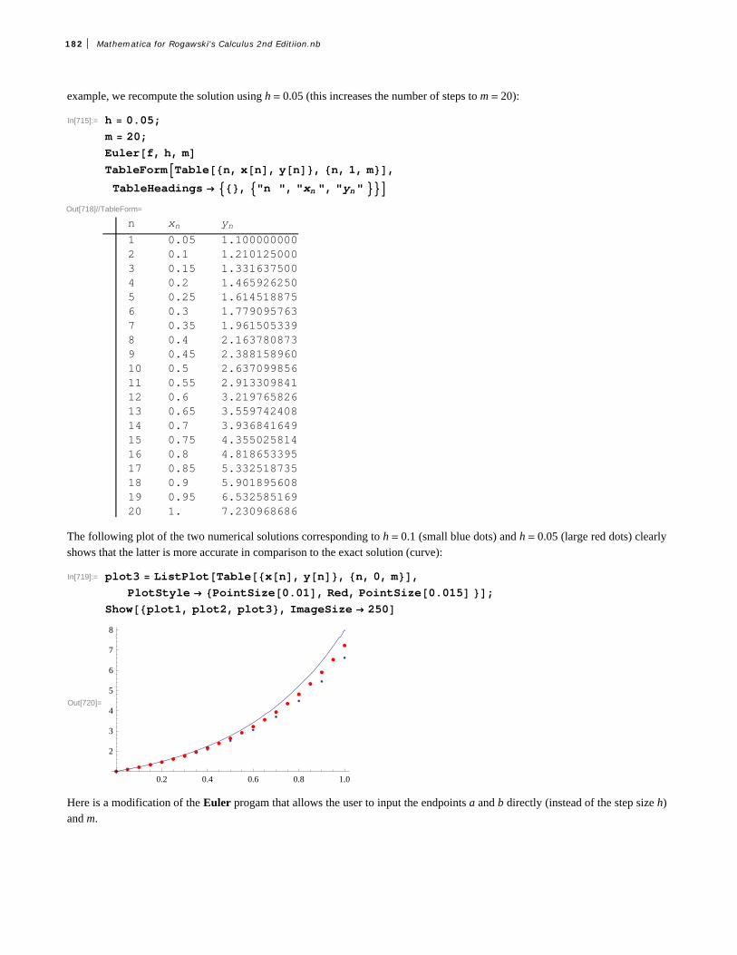
example, we recompute the solution using h = 0.05 (this increases the number of steps to m = 20):

In[715]:= h 0.05;m 20;Eulerf, h, mTableFormTablen, xn, yn, n, 1, m,TableHeadings , "n ", "xn ", "yn"


n xn yn

1 0.05 1.1000000002 0.1 1.2101250003 0.15 1.3316375004 0.2 1.4659262505 0.25 1.6145188756 0.3 1.7790957637 0.35 1.9615053398 0.4 2.1637808739 0.45 2.38815896010 0.5 2.63709985611 0.55 2.91330984112 0.6 3.21976582613 0.65 3.55974240814 0.7 3.93684164915 0.75 4.35502581416 0.8 4.81865339517 0.85 5.33251873518 0.9 5.90189560819 0.95 6.53258516920 1. 7.230968686

The following plot of the two numerical solutions corresponding to h = 0.1 (small blue dots) and h = 0.05 (large red dots) clearlyshows that the latter is more accurate in comparison to the exact solution (curve):

In[719]:= plot3 ListPlotTablexn, yn, n, 0, m,PlotStyle PointSize0.01, Red, PointSize0.015 ;

Showplot1, plot2, plot3, ImageSize 250

Out[720]=

0.2 0.4 0.6 0.8 1.0

2

3

4

5

6

7

8

Here is a modification of the Euler progam that allows the user to input the endpoints a and b directly (instead of the step size h)and m.


In[721]:= Clearf, x, y, h, a, b, mEulerEndptf_, a_, b_, m_ : Modulen, h, h N b a

m;

Doyn 1 SetPrecisionNyn h fxn, yn, 10;xn 1 xn h,n, 0, m

Example 9.8. For the differential equation y ' = x2 + 2 y, y0 = 1, approximate its solution over the interval 0, 2 using m = 10steps.

Solution: Again, we have f x, y = x2 + y, x0 = 0, y0 = 1. However, we now input the interval a, b = 0, 2 into EulerEndPt.

In[723]:= fx_, y_ : x2 y

m 10;x0 0;y0 1;

x0 x0;y0 y0;a 0;b 2;

In[731]:= EulerEndptf, 0, 2, mTableFormTablen, xn, yn, n, 1, m,TableHeadings , "n ", "xn ", "yn"


n xn yn

1 0.2 1.2000000002 0.4 1.4480000003 0.6 1.7696000004 0.8 2.1955200005 1. 2.7626240006 1.2 3.5151488007 1.4 4.5061785608 1.6 5.7994142729 1.8 7.47129712610 2. 9.613556552

This time we numerically compare the approximate solution with the exact solution:


In[733]:= Clearz, t, exactexact DSolvez't ft, zt, zx0 y0, zt, t;zt_ zt . exact1TableFormTablen, xn, yn, Nzx0 n b a m, n, 1, m,TableHeadings , "n ", "xn ", "yn", "yn"

Out[735]= 2 3 t 2 t t2


n xn yn yn1 0.2 1.200000000 1.224212 0.4 1.448000000 1.515473 0.6 1.769600000 1.906364 0.8 2.195520000 2.436625 1. 2.762624000 3.154856 1.2 3.515148800 4.120357 1.4 4.506178560 5.40568 1.6 5.799414272 7.09919 1.8 7.471297126 9.3089410 2. 9.613556552 12.1672

ü Exercises

In Exercises 1 through 4, plot the slope field of the given differential equations:1. y ' = x2 + y2 2. y ' = t2 y 3. y ' = sinx + y 4. y ' = x e-y

5. Consider the differential equation y ' = 3 y - 2 y2.a) Draw the slope field for the differential equation.b) Solve the differential equation.c) Assume y0 = 2. Plot the graph of the solution for this case and also the slope field on the same axes. Discuss the behavior ofthe solution as xØ¶.d) Redo part c) for the same differential equation but with initial condition given by ya = b (choose various values for a and b).

In Exercises 6 through 9, use Euler's Method to find a numerical solution to the given initial value problem along the statedinterval and using the prescribed number of steps. Also, find their exact solutions and compare the results.6. y ' = x2 - y, y0 = 1; 0, 1; m = 10 7. y ' = 1 - x2 cos y, y1 = 0; 1, 2; m = 208. y ' - y2 = x, y0 = 1; 0, 5;m = 50 9. y ' = -3 x 2 + lnx2 + y, y1 = 1; 1, 2; m = 100

10. Heun's method is a numerical method that improves on Euler's method. It uses the approximation from Euler's method as anauxiliary value (called a predictor), which we denote by yn+1

* :

yn+1* = yn + h f xn, yn

The actual approximation (called the corrector) is then computed as the mean of yn+1* (based on the slope of the tangent line at

xn, yn) and yn+1** = yn + h f xn+1, yn+1

* (based on the slope of the tangent line at xn+1, yn+1* ):

yn+1 =1

2yn+1* + yn+1

** = yn +1

2h f xn, yn + h f xn+1, yn+1

* a) Apply Heun's method to Exercise 6 and the compare the results obtained by Euler's method with the exact solution. Howmuch more accurate is Heun's method?b) Redo part a) using m = 20. How much more accurate is the solution compared to that for m = 10?


ü 9.4 The Logistic Equation


The differential equation

d y

d t= k y1 - y

A

is called the logistics equation. Here, k > 0 and A is a constant called the carrying capacity. This equation is useful for modelingthe growth of a population where resources are limited and can only sustain a certain maximum population given by the carryingcapacity.

Example 9.5. The population pt of mosquito larvae growing in a tree hole increases according to the logistics equation withgrowth constant k = 0.3 per day and carrying capacity A = 1000.

a) Assuming that the initial population of the larvae is 50, find the population pt at any time t. b) After how many days will the larvae population exceed 500?c) When does the larvae population reach 99% of the maximum capacity?

Solution:

a) We use k = 3

10 and solve the corresponding differential equation in Mathematica:

In[737]:= Clearysolde DSolvey't

3

10yt 1

yt1000

, y0 50, yt, t



Out[738]= yt 1000 3 t10

19 3 t10

NOTE: Be careful with using a decimal approximation for k. For example, try using k = 0.3 and see what happens.

Next, for convenience we write the solution given in the previous output as

In[739]:= Clearp, tpt_ solde1, 1, 2

Out[740]=1000 3 t10

19 3 t10

Thus, the population of larvae at any time t is given by

pt = 1000 e3 t10

19+e3 t10

b) To find how long it takes for the larvae population to reach 500, we solve

In[741]:= NSolvept 500, tNSolve::ifun : Inverse functions are being used by NSolve, so


Out[741]= t 9.8148, t 9.8148 20.944 , t 9.8148 20.944


Thus, it takes about ten days for the larvae population to exceed 500. Observe that p10 º 513.887.

NOTE: We ignored the other two solutions in the previous output since they are complex-valued and not physically relevant.

c) We first plot the graph of pt to estimate the number of days required for the larvae population to reach 99% of the maximumcapacity, that is, pt = 999.

In[742]:= Plotpt, t, 0, 60, ImageSize 250

Out[742]=

10 20 30 40 50 60

200

400

600

800

1000

It appears that the population reaches 999 larvae after t = 30. We use the Table command to numerically confirm this.

In[743]:= TableFormTablet, Npt, 20, t, 10, 50, 5,TableHeadings , "Days ", "Larvae Population"


Days Larvae Population10 513.8866830116854318815 825.7154653278878200720 955.0220053824840431625 989.6006793002358551430 997.6606988835103176735 999.4770810496474217340 999.8832735919316938645 999.9739524558509316550 999.99418788969128789

We can reasonably conclude from the table that the population reaches 999 larvae between 30 and 35 days. To obtain a moreprecise answer, we use Mathematica to solve pt = 999 for t:

In[744]:= NSolvept 999, tNSolve::ifun : Inverse functions are being used by NSolve, so


Out[744]= t 32.8373, t 32.8373 20.944 , t 32.8373 20.944 Thus, the desired time is approximately t = 33 days.

ü Exercises

1. A population of squirrels live in a forest with a carrying capacity of 3000. Assume logistic growth with growth constant k = 0.8per year.a) Find the population of the squirrels at any time t assuming an initial population of P0 = 800.b) How long will it take for the squirrel population to double? Triple?


2. From 1960 to 2000, the world's population doubled from approximately 3 billion to 6 billion people. Assuming that the humanpopulation follows logistic growth and that the earth has a carrying capacity of 100 billion people, determine the following:a) Find the population at any time t. What is the growth constant?b) What will the population be in the year 2050? How does this answer compare with projections from the United Nations?c) Find the year in which the human population will reach half its carrying capacity?d) When will the population grow the fastest, that is, the point on the graph where it changes from concave up to concave down(point of inflection)? What is the growth rate then?

3. In medicine, the logistics equation is used to model the growth of tumors in certain organs. Suppose a patient is diagnosedwith a tumor that has doubled in size to 2% of his liver when a year ago it only covered 1% of his liver. How long will it take thetumor to grow to 10% of his liver when a transplant will most like by required to increase his chances of survival.

4. The current population of a herd of bison living inside a national park is 1000. To ensure that the population does not reachmore than 1500 bison in 50 years time and 2000 bison in 100 years time, what carrying capacity should the park maintain?Assume that the bison population follows a logistics model.


Chapter 10 Infinite Series

ü 10.1 Sequences

Students should read Section 10.1 of Rogawski’s Calculus [1] for a detailed discussion of the material presented in thissection.

Recall that a sequence is a function whose domain is the set of non-negative integers.

In Mathematica, we denote a sequence an as a function. Thus, instead of an we write an. The limit of a sequence is evaluated by

using the Limit command. When Limit[a[n], nÆ•] is evaluated, Mathematica automatically assumes that n is a continuousvariable (instead of a discrete variable). It employs various techniques to evaluate limits.

To plot the graph of a sequence, we use the ListPlot command. ListPlot[list] plots the graph of list, where list is a list of points

x, y, denoted in Mathematica by {x,y}. In our case, list will be the table of values of the form {n,a[n]}. The corresponding plot

command in this case would be ListPlot[Table[{n,a[n]},{n,min,max}].

Example 10.1. Consider the sequence defined by

an =4 n+1

3 n+2

a) Find the first few terms of the sequence.

b) Plot the graph of the sequence.

c) Make a conjecture for the limit based on the graph.

d) Find the limit of the sequence.

Solution:

a) We define the sequence as a function of n and use the Table command to generate the first ten terms of the sequence.

In[745]:= Cleara, nan_ :

4 n 1

3 n 2


In[747]:= TableFormTablen, an, n, 1, 10,TableHeadings , "n", "an"


n an

1 1

2 98

3 1311

4 1714

5 2117

6 54

7 2923

8 3326

9 3729

10 4132

To obtain decimal expressions of these values, we evaluate

In[748]:= TableFormNTablen, an, n, 1, 10,TableHeadings , "n", "an"


n an

1. 1.2. 1.1253. 1.181824. 1.214295. 1.235296. 1.257. 1.260878. 1.269239. 1.2758610. 1.28125

b) To plot the graph of the sequence, we use the ListPlot command. Here is a plot of the first 100 terms of the sequence.


In[749]:= ListPlotTablen, an, n, 1, 100

Out[749]=

20 40 60 80 100

1.28

1.29

1.30

1.31

1.32

c) The graph suggests that the limit is 1.333 .... We can use the Table command to see this more clearly.

In[750]:= TableFormNTablen, an, n, 1000, 10000, 1000,TableHeadings , "n", "an"


n an

1000. 1.332782000. 1.333063000. 1.333154000. 1.333195000. 1.333226000. 1.333247000. 1.333258000. 1.333269000. 1.3332710000. 1.33328

Hence, the limit seems to be 1.3333... or 4/3. Here is a plot of y = 4 3 and the graph of the sequence for large values of n:


In[751]:= Clearplot1, plot2plot1 ListPlotTablen, an, n, 1, 1000, 10;plot2 Plot4 3, x, 1, 1000;Showplot1, plot2, PlotRange 1.25, 4 3

Out[754]=

200 400 600 800 1000

1.28

1.30

1.32

d) Finally, we confirm this in Mathematica by evaluating the limit as n goes to ¶.

In[755]:= Limitan, n Infinity

Out[755]=4

3

Example 10.2. Consider the sequence defined by

an =-1n

n

a) Plot the graph of the sequence.

b) Does the sequence converge?

Solution:

a) Again, we use ListPlot to plot the graph.


1nn



Out[758]=20 40 60 80 100

-0.10

-0.05

0.05

0.10

b) From the graph, it is clear that the sequence approaches 0 in the limit. We confirm this using the Limit command.

In[759]:= Limitan, n InfinityOut[759]= 0

NOTE: There are instances where the sequence an may not be well-defined if n is treated as a real variable (as opposed to aninteger variable). In such cases, Mathematica may return the limit unevaluated or else gives an output that indicates the limit maynot exist, as the following example illustrates.

Example 10.3. Determine whether or not the sequence defined below converges:

an = -1n n

n+1

Solution: First, we will plot the graph of the sequence.

In[760]:= Cleara, nan_ : 1n n

n 1


Out[762]=20 40 60 80 100

-1.0

-0.5

0.5

1.0

The graph clearly indicates the sequence does NOT converge (to a unique limiting value). We can see this by investigating thefollowing tables of values. The first one lists the even terms while the second one lists the odd terms of the sequence.


In[763]:= TableFormTablen, Na2 n, n, 10, 100, 10,TableHeadings , "n", "a2n"


n a2n

10 0.95238120 0.9756130 0.98360740 0.98765450 0.99009960 0.99173670 0.99290880 0.99378990 0.994475100 0.995025

In[764]:= TableFormTablen, Na2 n 1, n, 10, 100, 10,TableHeadings , "n", "a2n1"


n a2n1

10 0.9520 0.97530 0.98333340 0.987550 0.9960 0.99166770 0.99285780 0.9937590 0.994444100 0.995

Finally, let us evaluate the limit.

In[765]:= Limitan, n InfinityOut[765]= 2 Interval0,

This output, specifically the notation Interval[{0, p}], means that the limit does not exist uniquely, but has subsequences whose

limits take on the set of complex values e2 i x for all x œ 0, p. This is because the variable n that appears in the Limit command

is automatically assumed by Mathematica to be a complex variable. In our case, for n an integer variable, we have two subse-quences, a2 n and a2 n+1 (even and odd, respectively), converging to different limits (1 and -1, respectively). Thus, an diverges.

Example 10.4. Consider the sequence an defined recursively by a1 = 1 and an+1 = an + 1 . Generate the first ten terms ofthis sequence and compute its limit.

Solution: Here is one method of defining a recursive sequence.

In[766]:= Cleara, na1 1an_ : an Sqrtan 1 2

Out[767]= 1

NOTE: The second occurrence of a[n] in the preceding command tells Mathematica to store all intermediate values of the


recurrence in evaluating a[n].

Here are the first ten terms of the sequence:

In[769]:= TableFormTablen, an, n, 1, 10,TableHeadings , "n", "an"


n an

1 1

2 3

3 2 3

4 2 2 3

5 2 2 2 3

6 2 2 2 2 3

7 2 2 2 2 2 3

8 2 2 2 2 2 2 3

9 2 2 2 2 2 2 2 3

10 2 2 2 2 2 2 2 2 3

The following table gives decimal expressions of the same first ten terms and reveals the limit to be equal to 2.


In[770]:= TableFormTablen, Nan, n, 1, 10,TableHeadings , "n", "an"


n an

1 1.2 1.732053 1.931854 1.982895 1.995726 1.998937 1.999738 1.999939 1.9999810 2.

NOTE: In general, Mathematica is not able to directly compute limits of sequences defined recursively. Assuming an converges(prove this!), we then compute its limit, called L, say, by letting nØ¶ in the recurrence formula for an:

L = limnØ¶an = limnØ¶ an-1 + 2 = limnØ¶an-1 + 2 = L + 2

Solving the equation L = L + 2 then yields L = 2 as the limit.

In[771]:= SolveL SqrtL 2, LOut[771]= L 2

Example 10.5. Let a1 = 1 and b1 = 2 . Define two sequences recursively by

an+1 = an bn and bn+1 =an+bn

2

a) Choose various values of a1 and b1 and calculate the first ten terms of the sequences an and bn. b) Show that an § bn for every positive integer n.

c) Show that both sequences converge to the same limit. (NOTE: This common limit is called the arithmetic-geometric mean ofa1and b1.)

Solution:

a) Here is a program that generates the first ten values of an and bn.

In[772]:= Cleara, b, na1 1b1 10

ai_ : ai ai 1 bi 1 ;

bi_ : bi ai 1 bi 1

2;

Out[773]= 1

Out[774]= 10


In[777]:= TableFormTablek, Na k, 10, Nb k, 10, k, 1, 10 ,TableHeadings , "n", "an", "bn"


n an bn1 1.000000000 10.000000002 3.162277660 5.5000000003 4.170434885 4.3311388304 4.250027349 4.2507868585 4.250407086 4.2504071036 4.250407095 4.2504070957 4.250407095 4.2504070958 4.250407095 4.2504070959 4.250407095 4.25040709510 4.250407095 4.250407095

b) The following table suggests that an § bn for at least the first ten terms:

In[778]:= TableFormTablek, Na k, 10, Nb k, 10, Nbk, 10 Nak, 10, k, 1, 10 ,TableHeadings , "n", "an", "bn", "bnan"


n an bn bnan1 1.000000000 10.00000000 9.000000002 3.162277660 5.500000000 2.3377223403 4.170434885 4.331138830 0.1607039454 4.250027349 4.250786858 0.000759508

5 4.250407086 4.250407103 1.7 108

6 4.250407095 4.250407095 0. 1010

7 4.250407095 4.250407095 0. 1010

8 4.250407095 4.250407095 0. 1010

9 4.250407095 4.250407095 0. 1010

10 4.250407095 4.250407095 0. 1010

For a better feel on this, let us plot the graphs on the same axes. To this end, we define two lists using the Table command and

use the ListPlot command to plot the graphs.

In[779]:= plot1 ListPlotTablek, ak, k, 1, 10, PlotStyle Blue;plot2 ListPlotTablek, bk, k, 1, 10, PlotStyle Red;Showplot1, plot2, PlotRange 0, 10

Out[781]=

0 2 4 6 8 10

2

4

6

8

10


The above graph suggests that the two sequences converge to the same limit. Unfortunately, Mathematica's Limit commandcannot help us compute the limit of an and bn due to their recursive nature. (Try this!)

NOTE: We encourage the reader to experiment with different initial values for a1 and b1 to see if the sequences an and bn alwaysconverge to the same limit.

Example 10.6. Consider the sequence

an =n!1n

n

a) Show that if bn = ln an, then bn =ln n!-n ln n

n.

b) Does bn converge? If so, find the limit.

c) Does an converge? If so, find the limit.

Solution:

a) We define a sequence cn =ln n!-n ln n

n and then show that bn = cn.

In[782]:= Cleara, b, c

an_ :n1n

nbn_ : Logan

cn_ :Log n n Logn

n

In[786]:= TableFormTableNcn, Nbn, Ncn, 10 Nbn, 10, n, 2, 10,TableHeadings Automatic, " cn", " bn", " cnbn"


cn bn cnbn

1 0.346574 0.346574 0. 1011

2 0.501359 0.501359 0. 1010

3 0.591781 0.591781 0. 1010

4 0.65194 0.65194 0. 1010

5 0.695218 0.695218 0. 1010

6 0.72803 0.72803 0. 1010

7 0.753866 0.753866 0. 1010

8 0.774799 0.774799 0. 1010

9 0.792144 0.792144 0. 1010

The preceding table indicates that the two sequences are the same. Here is a plot of both:


In[787]:= ListPlotTablen, bn, n, 1, 100, Tablen, cn, n, 1, 100,PlotRange 1, 0.1, AxesOrigin 0, 0

Out[787]=

20 40 60 80 100

-1.0

-0.8

-0.6

-0.4

-0.2

This plot clearly shows that bn = cn, that is, lnan = ln n!1n

n = ln n!-n ln n

n. We leave it to the student to establish this equality

using properties of the natural logarithmic function.

b) The previous plot indicates that the limit of bn is -1. To confirm this, we use the Limit command.

In[788]:= Limitbn, n InfinityOut[788]= 1

c) Since bn = ln an, it follows that an = ebn and hence limnØ¶an = e-1. Again, we verify this using the Limit command:

In[789]:= Limitan, n Infinity

Out[789]=1

ü Exercises

In Exercises 1 though 3, determine the convergence of the given sequence.

1. an =3 n2+n+2

2 n2+12. an = ln 2 n+3

n+1 3. an = n

n

4. Let cn =1

n+1+ 1

n+2+ 1

n+3+ ... + 1

2 n.

a. Find the first ten terms of the sequence.b. Plot the graph of the sequence.c. Is the sequence increasing? Bounded? Convergent? Prove each of your assertions.d. Find limnØ¶ cn.

5. The nth harmonic number is defined to be the sum

Hn = 1 + 1

2+ 1

3+ ... + 1

n.

Let an = Hn - ln n and bn = 1

n+1 1

x„ x.

a. Show that Hn ¥ bn for n = 1, 2, 3, ..., 10. Prove that this holds for all positive integers n.

b. Show that an ¥ 0 for n = 1, 2, 3, ..., 10. Prove that this holds for all positive integers n.


c. Use the ListPlot command to plot the graph of an. Does the graph indicate that an is decreasing or increasing?

d. Evaluate limnØ¶an.

e. The limit in part d) is called Euler's Constant and is denoted by g. Compute g accurate to 20 digits.

ü 10.2 Infinite Series

Students should read Section 10.2-10.3 of Rogawski's Calculus [1] for a detailed discussion of the material presented inthis section.

ü 10.2.1 Finite Sums

Sum[a[n], n, n1, n2] evaluates the finite sum of an as n goes from n1 to n2.

Sum[a[n], n, n1, Infinity] evaluates the infinite series of an as n goes from n1 to ¶.

Using the BasicMathInput Palette, we can also enter finite sums or infinite series as nn1n2 an or nn1

an, respectively.

Example 10.7. Compute the following finite sums:

a) n=110 -1n

nb) k=1

5 k - 1 k + 1

c) k=130 20

k2k d) i=1

n 3 i - 2 e) k=010 k2+1

k3+2 k2+1

Solution:

a)

In[790]:= n1

10 1nn

Out[790]= 1627

2520

b)

In[791]:= Sumk 1 k 1, k, 1, 5Out[791]= 50

c) The binomial coefficient nm

= n!

m! n-m! is expressed in Mathematica by the command Binomial[n, m].

In[792]:= k0

30

Binomial30, k 2k

Out[792]= 205891132094649

NOTE: The above number is the same as 330 = 205 891 132 094 649. Verify this!

d)


In[793]:= j1

n

3 j 2

Out[793]=1

2n 3 n2

In[794]:= Simplify

Out[794]=1

2n 1 3 n

e)

In[795]:= k0

10 k2 1

k3 2 k2 1

Out[795]=361278549115758513

126627880430636728

ü 10.2.2 Partial Sums and Convergence

Example 10.8. Consider the series n=1¶ 1

4 n2-1. Let sn denote its nth partial sum.

a) Find s100. b) Compute every 10th partial sum up to n = 100.c) Compute every 1000th partial sum up to n = 10, 000.d) From the tables of values in parts a) and b) what do you infer about the convergence of the series? Prove your assertion.

Solution:

a) First, we define sn in Mathematica and then evaluate s100.

In[796]:= Clears, nsn_ :

j1

n 1

4 j2 1

s100

Out[798]=100

201

In[799]:= NOut[799]= 0.497512

b) Here, we use the command Table[s[n],{n,1,J,K}], which gives the list of every K-th value of sn, as n goes from 1 to J. The

command TableForm[N[Table[s[n],{n, 1, J, K }]]] lists the values in column form.

In[800]:= Tablesn, n, 1, 100, 10

Out[800]= 13,11

23,21

43,31

63,41

83,

51

103,

61

123,

71

143,

81

163,

91

183


In[801]:= NOut[801]= 0.333333, 0.478261, 0.488372, 0.492063,

0.493976, 0.495146, 0.495935, 0.496503, 0.496933, 0.497268In[802]:= TableFormTablen, Nsn, n, 10, 100, 10,

TableHeadings , "n", "sn"Out[802]//TableForm=

n sn

10 0.4761920 0.48780530 0.49180340 0.49382750 0.4950560 0.49586870 0.49645480 0.49689490 0.497238100 0.497512

c)

In[803]:= TableFormTablen, Nsn, n, 1000, 10000, 1000,TableHeadings , "n", " sn"


n sn

1000 0.499752000 0.4998753000 0.4999174000 0.4999385000 0.499956000 0.4999587000 0.4999648000 0.4999699000 0.49997210000 0.499975

d) It seems that the partial sums converge to 0.5. We confirm this by evaluating

In[804]:= Limitsn, n

Out[804]=1

2

Can you prove this? Hint: Use the method of partial fractions to decompose this series into a telescoping series as discussed inyour calculus text.

Example 10.9. Let sn be the nth partial sum of the harmonic series

k=1¶ 1

k.

a) Find s100. b) Compute every 1000th partial sum up to n = 10, 000c) Plot the graphs of the partial sums.


d) From the table of values in part (b) what do you infer? Prove your assertion.

Solution: We will follow the method of the preceding example. First, we define the nth partial sum.

In[805]:= Clears, nsn_ : Sum1 k, k, 1, n

a) Then s100 is given by

In[807]:= s100Out[807]= 14466636279520351160221518043104131447711

2788815009188499086581352357412492142272

In[808]:= NOut[808]= 5.18738

b) Here is a table of values of every 1000th term in the sequence sn for n less than or equal to 10, 000.

In[809]:= TableFormTablen, Nsn, n, 1000, 10000, 1000,TableHeadings , "n", " sn"


n sn

1000 7.485472000 8.178373000 8.583754000 8.871395000 9.094516000 9.276817000 9.430958000 9.564479000 9.6822510000 9.78761

c) Here is a plot of sn.

In[810]:= ListPlotTablen, sn, n, 1, 300, 20

Out[810]=

50 100 150 200 250

1

2

3

4

5

6

The graph above indicates a slow growth that makes it difficult to reach a definitive conclusion regarding the convergence of theharmonic series.

d) The table in b) and the plot in c) both suggest that the sequence of the partial sums is increasing. To convince ourselves of this,we compare s2n and n

2.


In[811]:= TableFormTablen 2., Ns2n, n, 1, 10,TableHeadings , " n

2", " s2n "

Out[811]//TableForm=n2

s2n

0.5 1.51. 2.083331.5 2.717862. 3.380732.5 4.05853. 4.743893.5 5.433154. 6.124344.5 6.816525. 7.50918

This table suggests that s2n ¥ n

2 for n ¥ 2. Use this fact (a proof of it can be found in your calculus text) to establish the diver-

gence of the harmonic series.

Example 10.10. Determine whether the following series converges or diverges.

a) n=1¶ -1n

n2b) j=1

¶ j-1

jc) n=1

¶ 1

n- 1

n+1 d) n=1

¶ lnn + 1 - ln n

Solution: In all cases, we let Mathematica attempt to evaluate the infinite sum. For those cases where Mathematica returns anumeric output, this is understood to mean that the series converges and that the sum of the series is the given value.

a)

In[812]:= n1

1nn2

Out[812]= 2

12

Thus, the series converges to - p2

12. To see this graphically, we plot the graph of the partial sums of the series using the ListPlot

command, along with the horizontal line representing its sum s = - p2

12º -0.822467.

In[813]:= Clears, n

sn_ k1

n 1kk2

;


In[815]:= plot1 ListPlotTablen, sn, n, 1, 100;

plot2 Plot 2

12, x, 1, 100;

Showplot1, plot2

Out[817]=

0 20 40 60 80 100

-0.8230

-0.8228

-0.8226

-0.8224

-0.8222

-0.8220

-0.8218

b) Observe that lim jØ¶j-1

j= 1 ∫ 0. Hence, the series does not converge according to the Test for Divergence. This explains the

following output message from Mathematica if we attempt to evaluate the series.

In[818]:= j1

j 1

j

Sum::div : Sum does not converge. à

Out[818]= j1

1 j

j

c) Since this is a telescoping series, it can be shown that the nth partial sum is given by sn = 1 - 1

n+1. This can be seen in the

following output:

In[819]:= sn_ : k1

n 1

k

1

k 1


In[820]:= TableFormTablen, sn, n, 1, 10,TableHeadings , "n", " sn"


n sn

1 1 1

2

2 1 1

3

3 12

4 1 1

5

5 1 1

6

6 1 1

7

7 1 1

2 2

8 23

9 1 1

10

10 1 1

11

Hence, the series converges to 1, which we confirm with Mathematica.

In[821]:= n1

1

n

1

n 1

Out[821]= 1

d) This, too, is a telescoping series with the nth partial sum given by sn = ln n + 1 (verify this). Hence, the series diverges, asshown by the following output.

In[822]:= n1

Logn 1 Logn


Out[822]= n1

Logn Log1 n

ü Exercises

1. Consider the series n=1¶ 1

n2+3 n+2.

a. Use the Apart command to decompose the terms of the series, an =1

n2+3 n+2, into partial fractions.

b. Use part (a) to find a formula for the nth partial sum of the series.

c) Is the series convergent? If so, then find its sum.

In Exercises 2 through 5, determine if the given series is convergent. If it is, then find its sum.


2. n=1¶ 1

nn+1 3. n=0¶ -1n

n!4. n=1

¶ -1n+1

5. The sereis n=0¶ a rn is called a geometric series.

a. Find the nth partial sum of the geometric series.b. For what values of r does the series converge? Diverge?c. Find the sum of the geometric series for those values where the series converges.

6. Consider the series n=1¶ 1

n3

.

a. Use the ListPlot command to plot the first ten partial sums of this series.

b. Show that the series converges.

ü 10.3 Tests for Convergence

Students should read Sections 10.4-10.5 of Rogawski's Calculus [1] for a detailed discussion of the material presented inthis section.

ü 10.3.1 Comparison and Limit Comparison Tests

The Comparison Test: Suppose 0 § an § bn for all n >M , where M is some positive integer.

a) If nã1¶ bn is convergent, then n=1

¶ an is also convergent.

b) If nã1¶ an is divergent, then n=1

¶ bn is also divergent.

The Limit Comparison Test: Suppose an and bn are both positive and limnØ¶an

bn= l. If 0 < l <¶ (i.e.,, if l is a finite positive

number), then n=1¶ an and n=1

¶ bn both converge or both diverge.

To test convergence of a given seriesn=1¶ an using the Limit Comparison Test, it is important that the series n=1

¶ bn easily be

checked for convergence.

Example 10.11. Discuss the convergence of the series

n=1¶ 1

n2+2

Solution: Since 1

n2+2

< 1

n2

= 1

n and the harmonic series n=1

¶ 1

n was shown to divergence in Example 10.8 of this text, it

follows by the Comparison Test that our series diverges also. This is verified by Mathematica:

In[823]:= n1

1

n2 2


Out[823]= n1

1

2 n2

Example 10.12. Discuss the convergence of the series


n=1¶ 3 n3+40 n2+4

n5+200 n4+1

Solution: To find another series to compare ours with, we consider one with terms bn =3

n2. This comes from considering lower

powers of n in both the numerator and denominator of an.

In[824]:= Cleara, b, n

an_ :3 n3 40 n2 4

n5 200 n4 1

bn_ :3

n2

In[827]:= Limit anbn , n Infinity

Out[827]= 1

Since the series n=1¶ 3

n2 is convergent (p-series) and limnØ¶

an

bn= 1, we conclude from the Limit Comparison Test that our series

n=1¶ 3 n3+40 n2+4

n5+200 n4+1 is also convergent.

Example 10.13. Discuss the convergence of the series n=1¶ 1 - cos 1

n.

Solution: We note that limnØ¶ 1 - cos 1

n = 0. This is confirmed by Mathematica.

In[828]:= Limit1 Cos1 n, n Out[828]= 0

Thus, the necessary condition for convergence is satisfied. But this does not guarantee convergence. We will use the ListPlotcommand to plot the graph of the partial sums to see if the series converges.

In[829]:= Clearssn_ : Sum1 Cos1 k, k, 1, n

In[831]:= ListPlotTablen, sn, n, 1, 100, PlotRange 0, 1

Out[831]=

0 20 40 60 80 100

0.2

0.4

0.6

0.8

1.0

The graph above clearly indicates convergence. To see that this is indeed true, we compare it with a series that is known to

converge: n=1¶ 1

n2. To this end, let us define an and bn as follows.


In[832]:= Cleara, b, nan_ : 1 Cos 1

n

bn_ :1

n2

Observe that both an and bn are positive terms for all n. Hence, we can apply Limit Comparison Test:


Out[835]=1

2

Therefore, the given series, n=1¶ 1 - cos 1

n, converges.

ü 10.3.2 The Integral Test

The Integral Test. Given an infinite series

n=1¶ an

we define f x so that f n = an . If f x is positive on the interval 1, ¶, decreasing on this interval, and if limxØ¶ f x = 0,then

1¶

f x „ x and n=1¶ an

both converge or both diverge.

Example 10.14. Use the integral test to determine the convergence of the following series.

a) n=1¶ 1

nc) j=1

¶ j e- j2 c) n=1¶ 1

n ln n

Solution:

a) Here, an =1

n and so we define f n in Mathematica:

In[836]:= Clearf, xfx_ :

1

x

In[838]:= f'x

Out[838]= 1

2 x32

Since f ' x < 0 for all x œ 1, ¶, it follows that f is decreasing. Clearly f is positive in value and limxØ¶ f x = 0. Thus we

can apply the Integral Test by evaluating 1¶

f x „ x:


In[839]:= Integratefx, x, 1, Infinity


x does not converge on 1,¶. à

Out[839]= 1

1

xx

To confirm this, we evaluate this improper integral according to its limit definition:

In[840]:= ClearF, bFb_ : Integratefx, x, 1, b

In[842]:= LimitFb, b Out[842]=

b) Here, we define f as

In[843]:= Clearf, xfx_ x Ex

2

Out[844]= x2x

In[845]:= Plotfx, x, 0, 5, PlotRange 0, 1

Out[845]=

0 1 2 3 4 5

0.2

0.4

0.6

0.8

1.0

The graph clearly shows that the function is decreasing. We can confirm this by solving

In[846]:= f'xSolvef'x 0

Out[846]= x2 2 x

2x2

Out[847]= x 1

2, x

1

2

In[848]:= f'1

Out[848]= 1


In[849]:= N1 Sqrt2Out[849]= 0.707107

Thus, f has critical points at ±1

2º 0.707. Since f ' 1 < 0, we conclude that f is decreasing on 1, ¶.

The graph also shows that limxØ¶ f x = 0. Again, we can confirm this by evaluating

In[850]:= Limitfx, x InfinityOut[850]= 0

Hence, the Integral Test can be used to determine if the series is convergent. That the series j=1¶ j e- j2 is convergent follows

from the fact that

In[851]:= 1

fx x

Out[851]=1

2

Since the corresponding integral is convergent, it follows that the series j=1¶ j e- j2 is also convergent.

c) In this case, we define f as

In[852]:= Clearf, xfx_

1

x Logx

Out[853]=1

x LogxIn[854]:= Plotfx, x, 2, 100

Out[854]=

20 40 60 80 100

0.04

0.06

0.08

0.10

0.12

0.14

We leave it for the reader to check that f satisfies all the conditions of the Integral Test, which we now apply.


In[855]:= 2

fx x


x Logx does not converge on 2,¶. à

Out[855]= 2

1

x Logxx

Since the preceding output states that the integral is divergent, we conclude that the corresponding series is divergent also.

Example 10.15. For what values of p does the series n=2¶ 1

nln np converge?

Solution: We apply the Integral Test. Toward this end, we define f x so that f n = 1

nln np and then verify that f x is positive

and decreasing on the interval a, ¶, and that limxØ¶ f x = 0:

In[856]:= Clearf, x, pfx_ :

1

x LogxpIn[858]:= Limitfx, x InfinityOut[858]= 0

To confirm this limit, we will plot graphs of f x for some values of p

In[859]:= PlotEvaluateTablefx, p, 4, 2, .5, x, 2, 100, PlotRange 0, 5

Out[859]=

0 20 40 60 80 100

1

2

3

4

5

In the plot above, observe that some of the graphs are initially increasing, but then begin to decrease at a certain point. Let usthen find the interval over which the function f x is decreasing for each p. To this end, we compute the derivative f ' x andsolve f ' x < 0 for x.

In[860]:= f'x

Out[860]= p Logx1p

x2Logxp

x2

In[861]:= Simplify

Out[861]= Logx1p p Logx

x2


In[862]:= Solvef'x 0, xOut[862]= x pSince (ln x-1-p > 0 for all x > 1, we see that f ' x < 0 if ln x > -p, or equivalently, x = ‰-p. Thus, f x is decreasing on 2, ¶where a is the maximum of 2 and ‰-p.

To apply the Integral Test, we integrate f over the interval 2, ¶. This is easier than integrating over the interval a, ¶, and

permissible since the integrals 2¶

f x „ x and a¶

f x „ x either converge or diverge together.

In[863]:= Integratefx, x, 2,

Out[863]= ConditionalExpressionLog21p

1 p, Rep 1

The preceding output shows that 2¶

f x „ x is convergent for p > 1. However, the case p § 1 remains unsolved. To evaluate the

integral in this situation, we define its anti-derivative Fb = 2b

f x „ x and find the limit of Fb as bØ ¶.

In[864]:= ClearF, bFb_ Integratefx, x, 2, b

Out[865]= ConditionalExpressionLog21p Logb1p1 p

, Reb 1 b Reals

Since b is a real number and b > 2 , the solution to our integral is the first one, that is, Fb = ln 21-p-ln b1-p

1-p, provided p ∫ 1. But

then for p < 1, we see that limbØ¶Fb =¶ since limbØ¶ lnb1-p =¶. For p > 1, we have limbØ¶Fb = ln 21-p

1-p, which we

already knew from the second previous Mathematica output. The following tables might be helpful to convince you about this.

In[866]:= TableLimitFb, b Infinity, p, 3, .9, .5Out[866]= , , , , , , , In[867]:= TableLimitFb, b Infinity, p, 1.1, 9, .5Out[867]= 10.3733, 2.0766, 1.3605, 1.12346, 1.02813, 0.997425, 1.0048, 1.03926,

1.09605, 1.1734, 1.27122, 1.39056, 1.53333, 1.70219, 1.90056, 2.13262For p = 1, we make this substitution inside the integral and evaluate it directly:

In[868]:= p 1;Integratefx, x, 2,


x Logx does not converge on 2,¶. à

Out[869]= 2

1

x Logx x

Therefore, the infinite series n=2¶ 1

nln np is convergent for p > 1 and divergent for p § 1.

NOTE: To see how slow the growth of this series is for the value of p = 1, we consider the following table of partial sums. Recallthat f n is the nth term of the series and hence the nth partial sum is given by


In[870]:= Clearp, s, nsn_ Sumfk, k, 2, n

Out[871]= k2

n Logkpk

The following output shows that the sum of the first ten thousand terms is only about 3.01501088.

In[872]:= p 1;

Ns10000Out[873]= 3.01501

Here is a plot of the graph of the first ten thousand partial sums in steps of 1,000.

In[874]:= ListPlotTablen, sn, n, 1000, 10000, 1000

Out[874]=

4000 6000 8000 10 000

2.80

2.85

2.90

2.95

3.00

ü 10.3.3 Absolute and Conditional Convergence

Suppose an > 0 for all n. The infinite series

n=1¶ -1n an

is called an alternating series. If the series n=1¶ -1n an is convergent but the series n=1

¶ an is divergent, then the alternating

series is called conditionally convergent. If n=1¶ an is convergent, then the alternating series n=1

¶ -1n an is called absolutely

convergent.

Alternating Series Test: If an is decreasing and limnØ¶an = 0, then the series n=1¶ -1n an is convergent.

Example 10.16. Determine if the given series is conditionally or absolutely convergent.

a) n=1¶ -1n

n2+1c) n=2

¶ -1n

n ln n

Solution:

a) We define an =1

n2+1 in Mathematica and check that an satisfies the conditions of the Alternating Series Test.


1

n2 1


In[877]:= Limitan, n Out[877]= 0

In[878]:= fx_ ax;f'x

Out[879]= 2 x

1 x22

Thus, an is decreasing since f ' x > 0, where f n = an. Moreover, an converges to 0. Hence, the series n=1¶ -1n

n2+1 is convergent

by the Alternating Series Test.

To check absolute convergence, we use the Limit Comparison Test with bn =1

n2.

In[880]:= Limit an1 n2

, n Infinity

Out[880]= 1


n2 is convergent and the previous output shows limnØ¶

an

bn= 1, we conclude that the series

n=1¶ an =n=1

¶ 1

n2+1 is also convergent. Therefore, the alternating series n=1

¶ -1n

n2+1 is absolutely convergent.

b) We procced as in part a).


1

n LognIn[883]:= Limitan, n Out[883]= 0

In[884]:= fx_ ax;f'x

Out[885]= 1

x2 Logx2

1

x2 Logx

For the same reasons we conclude that an is decreasing and converges to 0. Hence, the series n=2¶ -1n

n ln n is convergent by the

Alternating Series Test.

To check absolute convergence, we apply the Intgeral Test to f x:In[886]:= Clearm

Limit2

m

fx x, m InfinityOut[887]=

From this, we conclude that the series is conditionally convergent.

Example 10.17. Show that the series


n=1¶ -1n

n2+1

is conditionally convergent. Find a value of n for which the partial sum sn approximates the series by an error less than 10-5.Also, find the corresponding value for sn.

Solution: We leave it for the reader to check that the series converges conditionally as in the preceding example. For the secondpart of the problem, we proceed by first defining the partial sums of the series.

In[888]:= Clears, a, nan_ :

1

n2 1

sn_ : Sum1k ak, k, 1, nIf S denotes the sum of the alternating series, it can be shown that S - sn < an+1 (refer to your calculus text for a proof of thisfact). The following table of values gives some numerical evidence of this fact:

n1

1n

1 n2

In[891]:= TableNAbsn1

1n

n2 1

sm, Nam, m, 1, 10

Out[891]= 0.266189, 0.707107, 0.181024, 0.447214,0.135203, 0.316228, 0.107332, 0.242536, 0.088784, 0.196116,0.075615, 0.164399, 0.0658064, 0.141421, 0.0582284, 0.124035,0.0522031, 0.110432, 0.0473006, 0.0995037

In[892]:= ClearS, nS

n1

1n

n2 1

Out[893]= n1

1n

1 n2

The table below gives the values of an for large values of n.

In[894]:= TableNa10n , n, 1, 10 Out[894]= 0.0995037, 0.0099995, 0.001, 0.0001,

0.00001, 1. 106, 1. 107, 1. 108, 1. 109, 1. 1010

Thus, n = 106 is a possible value. But solving an = 10-5 can give us a more accurate value.

In[895]:= NSolveax 105, xOut[895]= x 100000., x 100000.Thus, if n = 100 001, we have S - sn < 10-5. We confirm this with Mathematica:


In[896]:= NS s100001Out[896]= 4.99993 106

Can you find a smaller value of n for which S - sn < 10-5?

ü 10.3.4 Ratio Test

The Ratio Test: Suppose an > 0 and let

r = limnØ¶an+1

an.

a) If r < 1, the series n=1¶ an converges.

b) If r > 1, the series n=1¶ an diverges.

c) If r = 1, no conclusion can be drawn about the convergence of the series n=1¶ an. In other words, if r = 1, then we must use

another test to determine the convergence.

Example 10.18. Use the Ratio Test to determine the convergence of the following series.

a) n=1¶ nn

n!c) j=2

¶ 1

j ln j3c) n=1

¶ 3 n3+40 n2+4

n5+200 n4+1

Solution: For each series, we define an to be its nth term and evaluate limnØ¶an+1

an.

a)


nn

n

In[899]:= Limitan 1 an, n Out[899]=

Since ‰ > 1, the series n=1¶ nn

n! converges by the Ratio Test.

b)

In[900]:= Cleara, jaj_ :

1

j Logj3Limitaj 1 aj, j

Out[902]= 1

This output means that we must use a different test. However, this is an instance of Example 11.12 in this text with p = 3. Hence,the series converges by the Integral Test.

c)

In[903]:= Cleara, n

an_ :3 n3 40 n2 1

n5 200 n4 1


In[905]:= Limitan 1 an, n Out[905]= 1

Again, this output means we are forced to use a different test. Therefore, we shall use the Limit Comparison Test instead. To this

end, we define bn =3

n2:

In[906]:= Clearb, nbn_ :

3

n2


Out[908]= 1


n2 is convergent, we conclude that the series n=1

¶ 3 n3+40 n2+4

n5+200 n4+1 is also convergent.

ü 10.3.5 Root Test

The Root Test: Suppose an > 0 and let

r = limnØ¶ an1n.

a) If r < 1, the series n=1¶ anconverges.

b) If r > 1, the series n=1¶ an diverges.

c) If r = 1, no conclusion can be drawn about the convergence of the series n=1¶ an. In other words, if r = 1, then we must use

another test to determine the convergence.

Example 10.19. Use the Root Test to determine the convergence of the following series:

a) n=1¶ n

2 n+1n

b) n=1¶ 1

n 3n+n2c) n=1

¶ 3 n+1

n2+n+1

Solution: For each series we define an to be its nth term and evaluate limnØ¶ an1n.

a)


n

2 n 1

n

In[911]:= Limitan1n, n

Out[911]=1

2

Thus, the series n=1¶ n

2 n+1n

converges by Root Test.

b)


1

n 3n n2


In[914]:= Limitan1n, n

Out[914]=1

3

Even though the preceding Limit command is returned as unevaluated, the N command reveals that it is approximately 1/3.

In[915]:= NOut[915]= 0.333333

To verify this, we use the Squeeze Theorem (discussed in your calculus text) with bn =1

2 n 3n and cn =1

n 3n . First, note that

bn § an § cn. We can verify this using the following plot:

In[916]:= Plot 3x

2 x, ax, 3x

x, x, 1, 10, PlotStyle Green, Red, Blue

Out[916]=

4 6 8 10

0.01

0.02

0.03

0.04

We now define bn and cn as and evaluate limnØ¶ cn1n and limnØ¶ bn1n.

In[917]:= Clearb, c, nbn_ :

1

2 n 3n

cn_ :1

n 3n

In[920]:= Limitbn1n, n InfinityLimitcn1n, n Infinity

Out[920]=1

3

Out[921]=1

3

Thus, we also have limnØ¶ an1n = 1

3 and hence the series converges by the Root Test.

c)


3 n 2

n2 n 1


In[924]:= Limit an1n, n Out[924]= 1

The Root Test fails. Let us try the Ratio Test:

In[925]:= Limit an 1an , n Infinity

Out[925]= 1

The Ratio Test fails as well. We can easily verify that the Integral Test is applicable. We will evaluate the integral

In[926]:= 1

ax x


1 - x + x2+

3 x

1 - x + x2 does not converge on 1,¶. à

Out[926]= 1

2 3 x

1 x x2x

To confirm the divergence of the improper integral, we leave it to the reader to evalaute the function Fx defined below for largevalues of x.

In[927]:= ClearF, bFb_ :

1

b

ax x

ü Exercises

In Exercises 1 through 6, use the Comparison Test or the Limit Comparison Test to determine if the given series is convergent. Ifit is convergent, then find its sum.

1. n=1¶ n

n3+1

2. n=2¶ ln n

n2+3 ln n3. n=1

¶ n4+200 n2+1000 n+2222

n6+5 n4+n+1

4. n=1¶ ln n

n2 5. n=2

¶ 1

nln n6. n=1

¶ 1 - 2-1n

In Exercises 7 through 9, use the Integral Test to determine if the given series is convergent. If it converges, then find its sum.

7. n=1¶ n

n2+18. n=2

¶ n

2n 9. n=1¶ ln n3

n2

10. For what values of p does the series n=1¶ 1

np ln n converge?

11. Consider the series n=2¶ ln nk

np .

a. Fix a value of p (say, p = 2 or p = 1 2) and find all values of k for which the series converges.

b. Fix a value of k (say, k = 2 or k = -2) and find all values of p for which the series converges.

c. Generalize the results of a) and b) to all values of p and k.

12. Let f be a positive valued function that decreases on 1, ¶ and let an = f n. It can be shown that


1

¶f x „ x §n=1

¶ an § a1 + 1

¶f x „ x .

a. Use f x = 1

x1.1 to verify this.

b. Approximate n=1¶ 1

n1.1 using its nth partial sums with n = 10, 100, 1000, 10 000.

In Exercises 13 through 16, determine if each of the infinite series is absolutely convergent, conditionally convergent, or diver-

gent. Justify your conclusions!

13. n=1¶ -1n n2-1

n2+114. n=1

¶ 20 n2-n-1

n3+n2+3315. n=1

¶ -2n

n!16. n=1

¶ -1n+1 n + 1 - n ]

17. Discovery Exercise:

a. Determine the convergence or divergence of n=2¶ 1

n ln ln ln n0.5, n=2

¶ 1

n ln ln ln n , and n=2¶ 1

n ln ln ln n2.

b. Generalize your work in part a) by determining for which real numbers p the seriesn=2¶ 1

n ln ln ln np converges.

In Exercises 18 through 25, determine the convergence or divergence of the given infinite series using any of the convergencetests discussed in this section.

18. n=1¶ 3 n+1

4 n+519. n=1

¶ n

2 n2+1 20. n=1

¶ n+3

4 n3+5 21. n=1

¶ n 2

3n

22. n=1¶ n 3

2n

23. n=1¶ nn

n!24. n=1

¶ n!2

3 n! 25. n=0¶ -1n 1 + 1

nn

26. The Ratio Test proved to be inconclusive for some of the series in the previous exercise. Can you conjecture for what type ofseries the Ratio Test will fail in general? Use other tests to rework the problems in the first exercise where the Ratio Test failed.

27. Of the following four conditions, one guarantees that a series will diverge, two conditions guarantee that a series will con-verge, and one has no guarantee (the series can either converge or diverge). Identify each one and explain your reasoning.

limnØ¶an+1

an= 0

limnØ¶an+1

an= 1

2

limnØ¶an+1

an= 1

limnØ¶an+1

an= 2

28. Identify the two series that are the same:

a. n=1¶ n 3

4n

b. n=0¶ n + 1 3

4n

c. n=1¶ n 3

4n-1

In Exercises 29 through 32, determine the convergence or divergence of the series:

29. n=1¶ 2 n

n

+1) n 30, n=0¶ e-n 31. n=1

¶ -2 n

3 n+13 n

32. n=1¶ n

2 n+1) n

33. Construct two examples of infinite series, the first convergent and the second divergent, for which the Root Test generatesinconclusive information.

34. Use the Root Test to test for convergence or divergence of the series:


a. 1

ln 33+ 1

ln 44+ 1

ln 55+ 1

ln 66+ ...

b. 1+ 2

3+ 3

32+ 4

33+ 5

34+

6

35+...

Hint: Write a formula for the general nth term in each case.

ü 10.4 Power Series


ü 10.4.1 Taylor Polynomials

The Taylor polynomial of a given function f at a point x = a is given by

Tnx = f a + f ' a x - a + f '' a2!

x - a2 +f ''' a

3!x - a3 + ....+

f nan!

x - an.

The Mathematica Series[f,{x, a, n}] generates the nth Taylor polynomial Tnx plus a term of the form Oxn+1. To obtain the

Taylor polynomial without this term, we use the command Normal[Series[f,{x, a, n}]].

The nth remainder Rnx of f x at x = a is defined by

Rnx = f x - Tnx.Taylor's Theorem states that

Rnx = 1

n! a

xf n+1u x - un „u.

Here is a way to define the Taylor polynomial of f at x = a by defining Tnx and the nth remainder Rnx (using Taylor's Theo-

rem for Rn) without referring to Mathematica's built-in command Series.

In[929]:= Cleara, x, f, T, RTx_, a_, n_ :

k0

n Dfx, x, k . x a

kx ak

Rx_, a_, n_ :1

na

x

Dfu, u, n 1 x un u

Example 10.20. Let f x = ex. Find its 5th Taylor polynomial at x = 0.

Solution: We use the Series command to obtain the answer:

In[932]:= NormalSeriesEx, x, 0, 5

Out[932]= 1 x x2

2x3

6x4

24

x5

120

Using the polynomial Tx, a, n, we defined above we get


In[933]:= Clearffx_ : Ex

Tx, 0, 5

Out[935]= 1 x x2

2x3

6x4

24

x5

120

In[936]:= Rx, 0, 5

Out[936]=1

120120 120 x 120 x 60 x2 20 x3 5 x4 x5

Example 10.21. Find the nth Taylor polynomial of f x at x = a for various values of a and n.

a) f x = x b) f x = cos x

Solution: a) We shall use the same function T[x,a,n] defined in the previous example (make sure you evaluate this functionbefore you evaluate the table below).

In[937]:= Cleara, x, fTx_, a_, n_ :

k0

n Dfx, x, k . x a

kx ak

Rx_, a_, n_ :1

na

x

Dfu, u, n 1 x un u

In[940]:= Clearffx_ x

TableFormTable Tx, a, n , a, 1, 5, n, 1, 3 ,

TableHeadings

"at a=1", "at a=2", "at a=3", "at a=4", "at a=5", "n=1", "n=2", "n=3"Out[941]= x


n=1 n=2 n=3

at a=1 1 121 x 1 1

21 x 1

81 x2 1 1

21 x 1

81 x2 1

161

at a=2 2 2x

2 22 2x

2 2 2x2

16 22 2x

2 2 2x2

16 2 2x3

64 2

at a=3 3 3x

2 33 3x

2 3 3x2

24 33 3x

2 3 3x2

24 3 3x3

144 3

at a=4 2 144 x 2 1

44 x 1

644 x2 2 1

44 x 1

644 x2 1

5124

at a=5 5 5x

2 55 5x

2 5 5x2

40 55 5x

2 5 5x2

40 5 5x3

400 5

b) We proceed as in part a):


In[943]:= Clearffx_ CosxTableFormTable Tx, a, n , a, 0, 2 Pi, Pi 2, n, 1, 4 ,

TableHeadings "at a=0", "at a=/2", "at a=", "at a=3/2", "at a=2","n=1", "n=2", "n=3", "n=4"

Out[944]= CosxOut[945]//TableForm=

n=1 n=2 n=3 n=4

at a=0 1 1 x2

21 x2

21 x2

2 x4

24

at a=/2

2 x

2 x

2 x 1

6

2 x3

2 x 1

6

2 x3

at a= 1 1 12 x2 1 1

2 x2 1 1

2 x2 1

24

at a=3/2 3 2 x 3

2 x 3

2 x 1

6 3

2 x3 3

2 x 1

6 3

2 x3

at a=2 1 1 122 x2 1 1

22 x2 1 1

22 x2 1

242

Example 10.22. Let f x = 1

2+3 x2.

a) Find the Taylor polynomials Tnx of f at x = 0 for n = 1, 2, ..., 6.b) Draw the graphs of the function f and its Taylor polynomials found in part a).c) Over which interval does the nth Taylor polynomial gives a close approximation to f x if n = 4, n =10, and n = 20?

Solution:

a) Here are the Taylor polynomials up to order n = 6.

In[946]:= Clearffx_

1

2 3 x2

TableFormTable n, Tx, 0, n , n, 1, 6 ,

TableHeadings , "n", "Tn at a=0"

Out[947]=1

2 3 x2


n Tn at a=0

1 12

2 12 3 x2

4

3 12 3 x2

4

4 12 3 x2

4 9 x4

8

5 12 3 x2

4 9 x4

8

6 12 3 x2

4 9 x4

8 27 x6

16

b) We first use the Plot command to plot the graphs of f and its Taylor polynomial at x = 0 for the desired values of n. We then

use the Show command to plot both graphs on the same axes.


In[949]:= Clearplot1, plot2plot1 Plotfx, x, 3, 3, PlotStyle Red;plot2 PlotEvaluateTableTx, 0, n, n, 1, 6, x, 3, 3 ;Showplot1, plot2

Out[952]=

-3 -2 -1 1 2 3

0.1

0.2

0.3

0.4

0.5

c) We use the same commands as in part b) except that we do not use the Table command. The first one is for the case n = 4.

In[953]:= Clearplot1, plot2plot1 Plotfx, x, 3, 3, PlotStyle Red;plot2 PlotEvaluateTx, 0, 4, x, 3, 3 ;

Showplot1, plot2

Out[956]=

-3 -2 -1 1 2 3

0.1

0.2

0.3

0.4

0.5

It seems that the two graphs are close to each other if x is in the interval -0.5, 0.5. To see this close up, we recommend thatyou change the range of values for x in both plots (plot1 and plot2) to the interval -1, 1. We can confirm this by plotting the 4thremainder of f x at x = 0.


In[957]:= PlotEvaluateRx, 0, 4, x, 1, 1, PlotRange 1, 1

Out[957]=-1.0 -0.5 0.5 1.0

-1.0

-0.5

0.5

1.0

We repeat the above with n = 10.

In[958]:= Clearplot1, plot2plot1 Plotfx, x, 3, 3, PlotStyle Red;plot2 PlotEvaluateTx, 0, 100, x, 3, 3 ;

Showplot1, plot2

Out[961]=

-3 -2 -1 1 2 3

0.1

0.2

0.3

0.4

0.5

The graph above clearly indicates the 10th Taylor polynomial gives a close approximation for f in the interval -.6, .6. Again,plotting Rn will confirm this.



Out[962]=-1.0 -0.5 0.5 1.0

-1.0

-0.5

0.5

1.0

If we continue in this manner, we see that the Taylor polynomial Pn for large values of n gives a better approximation of f in theinterval -1, 1. In fact, for n = 20, we see that Rnx is almost zero in the interval -0.7, 0.7, which is an improvement over theprevious interval -0.6, 0.6 obtained for n = 10.


Out[963]=-1.0 -0.5 0.5 1.0

-1.0

-0.5

0.5

1.0

ü 10.4.2 Convergence of Power Series

A series of the form

n=0¶ anx - x0n = a0 + a1x - x0 + a2x - x02 + a3x - x03 + ....

is called a power series.

The set of all x for which the series converges is called the interval of convergence.

If the series converges for x = x0 only, we say is radius of interval is R = 0. In this case, its interval of convergence is x0.If the series converges for all real numbers x, we say its radius of convergence is R =¶. In this case, its interval of convergenceis -¶, ¶.


If the series converges for some x ∫ x0 and diverges for some y, then it can be shown that there exists R > 0 such that the powerseries converges for all x for which x - x0 < R and diverges for all x for which x - x0 > R. The convergence at x = x0 - Rand x = x0 + R needs to be checked.

When the radius of convergence R is a positive real number, there are four possiblities for the interval of convergence:

x0 - R, x0 + R or x0 - R, x0 + R or x0 - R, x0 + R or x0 - R, x0 + R depending on the convergence at the end points of the intervals.

The radius of convergence R of the power series n=0¶ anx - x0n can be found by using the Ratio or Root Test. Let

r = limnØ¶an+1

an or r = limnØ¶ an

n

a) If r = 0, then R =¶. b) If r =¶, then R = 0 .

c) If 0 < r <¶, then R = 1

r.

Example 10.23. Find the radius and interval of convergence for the given power series.

a) n=0¶ n

2 n+1xn b) n=1

¶ x-3n

n 3n c) n=0¶ x+2n

n2+n+1

d) n=0¶ nn xn e) n=0

¶ 1

n!x - 1n

Solution:

a) Let us define smx to be the mth partial sum of the series and plot the graph of some of these partial sums. We will plot every100th partial sum up to 10,000 terms.

In[964]:= Clears, n, msx_, m_ :

n0

m n

2 n 1xn

In[966]:= PlotEvaluateTablesx, m, m, 1, 1000, 100, x, 2, 2

Out[966]=

-2 -1 1 2

-2μ1026

2μ1026

4μ1026

This clearly indicates that the partial sums diverge outside -1, 1. Here is the plot over the interval -1, 1.


In[967]:= PlotEvaluateTablesx, m, m, 1, 1000, 100, x, 1, 1

Out[967]=

-1.0 -0.5 0.5 1.0

0.5

1.0

1.5

We now use calculus. Here, note that an =n

2 n+1 and x0 = 0. We first define an in Mathematica and find the radius of conver-

gence. We recall a (absolute value of a) is entered as Abs[a].

In[968]:= Cleara, n, ran_ :

n

2 n 1

In[970]:= r LimitAbsan 1an , n Infinity

Out[970]= 1

Thus, the radius of convergence is R = 1

r= 1

1= 1. The power series convrges on -1, 1. To check convergence at the endpoints

x = -1 and x = 1, we note that the power series becomes n=0¶ n

2 n+1-1nand n=0

¶ n

2 n+11n, both of which are divergent, since

their nth terms do not converge to 0. Here, Mathematica confirms the divergence at the endpoints.

In[971]:= n0

n

2 n 11n


Out[971]= n0

1n n1 2 n

In[972]:= n0

n

2 n 11n


Out[972]= n0

n

1 2 n

Therefore, the interval of convergence is -1, 1.

b) n=1¶ x-3n

n 3n


In[973]:= Cleara, r, nan_ :

1

n 3n

In[975]:= r Limit an 1an , n Infinity

Out[975]=1

3

Thus the radius of convergence is R = 1

r= 1

13 = 3.

Since x0 = 3, the power series converges on x0 - R, x0 + R = 3 - 3, 3 + 3 = 0, 6. We need to check the endpoints x = 0 andx = 6. We substitute these in the power series and evaluate

In[976]:= n1

x 3nn 3n

. x 0, 6

Out[976]= Log2, Thus, the interval of convergence is 0, 6.

c) n=1¶ x+2n

n2+n+1


1

n2 n 1

In[979]:= r LimitAbs an 1an , n

Out[979]= 1

Hence, the radius of convergence is R = 1

1= 1. Since x0 = -2, we see that the power series converges at least on the open interval

-2 - 1, -2 + 1 = -3, -1. To determine the actual interval of convergence we need to check the endpoints. As in part c), weevaluate

In[980]:= n0

x 2nn2 n 1

. x 3, 1

Out[980]= HypergeometricPFQ1, 113, 123, 32 3

2,3

2 3

2, 1,

HypergeometricPFQ1, 113, 123, 32 3

2,3

2 3

2, 1

In[981]:= NOut[981]= 0.76131 4.70246 1016 , 1.79815 4.96787 1016 Since this is not clear, we examine the series by plugging in by hand x = -3 and x = -1. When x = -3 the series becomes

n=1¶ -3+2n

n2+n+1= n=1

¶ -1n

n2+n+1, which is an alternating series. We leave it to the reader to verify that the Alternating Series Test

applies in this case. Thus, we have a convergent series.


Next, we substitute x = -1 to obtain the series n=1¶ -1+2n

n2+n+1= n=1

¶ 1

n2+n+1 to which we apply the Integral Test (verify that the

conditions of the Integral Test are satisfied):

In[982]:= Integrate 1

x2 x 1, x, 0, Infinity

Out[982]=2

3 3

Thus, the series converges in this case as well. Therefore, the interval of convergence for the power series is -3, -1. d) n=0

¶ nn xn

In[983]:= Cleara, r, nan_ : nn


Out[985]=

Thus, the radius of convergence is R = 0 and the series converges for x = 0 only.

e) n=0¶ 1

n!x - 1n


1

n


Out[988]= 0

Thus, the radius of convergence is R =¶ and the series converges for all real x. Hence, the interval of convergence is -¶, ¶.

ü 10.4.3 Taylor Series

The Taylor series for f x at x = a is given by the power series

n=0¶ f na

n!x - an = f a + f ' a x - a + f '' a

2x - a2 +

f ''' a6

x - a3 + .....

The Mathematica command Series[f,{x, a, n}] generates the power series of f at x = a to the order x - an. It is not possible towrite all the terms explicitly since there are infinitely many.

Example 10.24. Let f x = 1+x

1+x2.

a) Find the first ten terms of the Taylor series of f at x = 0.b) Estimate the radius and interval of convergence of the Taylor series of f at x = 0.

Solution:

a) We use the Series command to obtain the Taylor series as follows:


In[989]:= Clearf, xfx_ :

1 x

2 x

In[991]:= Seriesfx, x, 0, 10

Out[991]=1

23 x

43 x2

83 x3

163 x4

323 x5

643 x6

1283 x7

2563 x8

512

3 x9

10243 x10

2048 Ox11

This output gives the Taylor series to order n = 10.

b) To first gain intuition for the radius of convergence of the Taylor series, we define the nth Taylor polynomial of f x as a

function of n (note our use of the Normal command to truncate the remainder term from the Taylor series).

In[992]:= ClearT, x, nTx_, n_ : NormalSeriesfx, x, 0, n

Here is a list of the first 20 of these polynomials.

In[994]:= TableTx, n, n, 0, 10

Out[994]= 12,1

23 x

4,1

23 x

43 x2

8,1

23 x

43 x2

83 x3

16,

1

23 x

43 x2

83 x3

163 x4

32,1

23 x

43 x2

83 x3

163 x4

323 x5

64,

1

23 x

43 x2

83 x3

163 x4

323 x5

643 x6

128,1

23 x

43 x2

83 x3

163 x4

323 x5

643 x6

1283 x7

256,

1

23 x

43 x2

83 x3

163 x4

323 x5

643 x6

1283 x7

2563 x8

512,

1

23 x

43 x2

83 x3

163 x4

323 x5

643 x6

1283 x7

2563 x8

512

3 x9

1024,

1

23 x

43 x2

83 x3

163 x4

323 x5

643 x6

1283 x7

2563 x8

512

3 x9

10243 x10

2048

Observe that each polynomial appears twice, that is, T2 n = T2 n+1, since f is an even function. Next, we plot the graphs of someof these polynomials:


In[995]:= Clearplot1plot1

PlotEvaluateTableTx, n, n, 1, 20, x, 5, 3, PlotRange 10, 10

Out[996]=-4 -2 2

-10

-5

5

10

To compare the graph of these polynomials, we plot the graph of f and use the Show command.

In[997]:= Clearplot2plot2 Plotfx, x, 5, 3, PlotRange 10, 10, PlotStyle Red

Out[998]=-4 -2 2

-10

-5

5

10


In[999]:= Showplot1, plot2, PlotRange 10, 10

Out[999]=-4 -2 2

-10

-5

5

10

Observe that the graphs of the Taylor polynomials in the preceding plot seem to give a good approximation to f only inside theinterval -2, 2. This suggests that the radius of convergence is 2. This becomes more evident as we plot the graph of Tn forlarge values of n as shown in the following plot, where n = 30, 35, 40, 45, 50.

In[1000]:= Clearplot3plot3 PlotEvaluateTableTx, n, n, 30, 50, 5, x, 3, 3;plot4 Plotfx, x, 5, 3, PlotStyle Red, Thickness0.002;Showplot3, plot4, PlotRange 10, 10

Out[1003]=-4 -2 2

-10

-5

5

10

To prove that the radius of convergence is indeed R = 2, we first find a formula for the Taylor coefficients. Based on the follow-

ing table, it is clear that a0 = 1 2 and an = -1n 32n+1 (prove this for all n).

In[1004]:= an_ : Dfx, x, n n . x 0

Tablean, n, 0, 10

Out[1005]= 12,

3

4,3

8,

3

16,

3

32,

3

64,

3

128,

3

256,

3

512,

3

1024,

3

2048

We now apply the Ratio Test on n=0¶ an xn.


In[1006]:= Clearaan_ 1^n 3 2^n 1r LimitAbsan 1

an , n

Out[1007]= 3 1n 21n

Out[1008]=1

2

Hence, the radius of convergence is R = 1 r = 2.

Next, we determine whether the endpoints should be included in the interval of convergence. For this, we evaluate our Taylorseries at x = -2 and x = 2.

In[1009]:= n1

an 2^n

n1

an 2^n


Out[1009]= n1

3

212 n


Out[1010]= n1

3 1n2

This shows that the Taylor series diverges at both endpoints. Thus, the interval of convergence is -2, 2. Example 10.25. Let f x = sin x.

a) Find the Taylor series of f at x = 0.b) Find the radius and interval of convergence of the Taylor series.

Solution:

a) We repeat the steps in the previous example.

In[1011]:= Clearffx_ : Sinx

In[1013]:= ClearTTx_, n_ : NormalSeriesfx, x, 0, n

In[1015]:= TableTx, n, n, 0, 10

Out[1015]= 0, x, x, x x3

6, x

x3

6, x

x3

6

x5

120, x

x3

6

x5

120, x

x3

6

x5

120

x7

5040,

x x3

6

x5

120

x7

5040, x

x3

6

x5

120

x7

5040

x9

362880, x

x3

6

x5

120

x7

5040

x9

362880


Observe that all terms of the Taylor polynomials are odd powers of x. Can you explain why?

Here is a plot of the graphs of the first ten of these polynomials and the function f .

In[1016]:= Clearplot1, pl0t2plot1 PlotEvaluateTableTx, n, n, 0, 10, x, 3 Pi, 3 Pi;plot2 Plotfx, x, 3 Pi, 3 Pi, PlotStyle Red;Showplot1, plot2, PlotRange 10, 10

Out[1019]=-5 5

-10

-5

5

10

b) Observe that the higher the order of the Taylor polynomial the better it approximates f over a wider interval. To see this moreclearly, we plot Tn for n = 20, 40, 60.

In[1020]:= Clearplot1, plot2plot1 Plotfx, x, 40, 40, PlotStyle Red, PlotRange 5, 5;plot2

Plot EvaluateTx, 20 , x, 40, 40 , PlotStyle Blue, PlotRange 5, 5;plot3 Plot EvaluateTx, 40 , x, 40, 40 ,

PlotStyle Blue, PlotRange 5, 5;plot4 Plot EvaluateTx, 60 , x, 40, 40 ,

PlotStyle Blue, PlotRange 5, 5;Showplot1, plot2

Out[1025]=-40 -20 20 40

-4

-2

2

4



Out[1026]=-40 -20 20 40

-4

-2

2

4


Out[1027]=-40 -20 20 40

-4

-2

2

4

The preceding plots suggest that the radius of convergence for the Taylor series of sin x is R =¶. To prove this, we first find aformula for the Taylor coefficients an. Again, based on the following table, it is clear that an = sinp n 2 n ! (prove this for alln).

In[1028]:= an_ : Dfx, x, n n . x 0

Tablean, n, 0, 10

Out[1029]= 0, 1, 0, 1

6, 0,

1

120, 0,

1

5040, 0,

1

362880, 0

We now apply the Root Test on n=0¶ an xn.


In[1030]:= Cleara, n, ran_ SinPi n 2 nTablean, n, 0, 10r LimitAbsan^1 n, n

Out[1031]=

Sin n 2

n

Out[1032]= 0, 1, 0, 1

6, 0,

1

120, 0,

1

5040, 0,

1

362880, 0

Out[1033]= 0

Hence, the radius of convergence is R =¶.

ü Exercises

In Exercises 1 through 6, determine the radius and interval of convergence for the given power series.

1. n=1¶ -1n+1 xn

4n 2. n=0¶ 2 n ! x

2) n 3. n=1

¶ n! xn

2 n!4. n=0

¶ -1n xn

n+15. n=0

¶ 4 xn 6. n=0¶ 2 xn

n!

7. Give examples of power series that have an infinite radius of convergence, a radius of convergence containing only the center,and a radius of convergence of one.

8. Find the Taylor series for f x = e2 x centered about c = 0.

9. Find the Taylor series for f x = ln x centered about the point c = 1.

In Exercises 10 through 12, find the MacLaurin series for each of the given function.

10. f x = sin 2 x 11. gx = sinh x 12. hx = arc sin x x

13. Consider the function f x = e-1x2if x ∫ 0

0 if x = 0.

a. Plot the graph of this function using Mathematica.b. Use the limit definition of the derivative and L'Hopital's Rule to show that every higher-order derivative of f at x = 0 vanishes.c. Find the MacLaurin series for f . Does the series converge to f ?

14. Use Taylor series to evalaute the following definite integral, which cannot be integrated via elementary means:

0

1 sin x

x„ x.

15. Find the following limit using the theory of Taylor series.

lim xØ 0 1-cos x

x


Chapter 11 Parametric Equations, Polar Curves, and Conic Sections

ü 11.1 Parametric Equations


Parametric equations are useful for describing curves not modeled by functions or motions parametrized by quantities such astime. The standard form for a set of parametric equations is

xt = f tyt = gt

where t is called the parameter.

ü 11.1.1. Plotting Parametric Equations

The Mathematica command for plotting a curve defined by parametric equations x = f t and y = gt for a § t § b is Parametric-

Plot[{f(t),g(t)},{t,a,b}].

Here are some examples:

Example 11.1. Plot the curve described by the parametric equations x = cos t and y = sin t for 0 § t § 2 p.

Solution:

In[1034]:= ParametricPlotCost, Sint, t, 0, 2 , ImageSize 200

Out[1034]=-1.0 -0.5 0.5 1.0

-1.0

-0.5

0.5

1.0

NOTE: Recall that the above parametric equations represent the unit circle. However, Mathematica may produce a graph that,depending on its default settings, looks visually like an ellipse due to different scalings of the x- and y-axes. In that case, the plot

option AspectRatio can be used to specify the ratio of the height to the width for a plot. For example, to stretch the plot above so

that the circle becomes elliptical where the height is twice as long as the width, we can set AspectRatio equal to 2.


In[1035]:= ParametricPlotCost, Sint, t, 0, 2 , AspectRatio 2, ImageSize 200

Out[1035]=-1.0 -0.5 0.5 1.0

-1.0

-0.5

0.5

1.0

Example 11.2. Plot the curve described by the parametric equations x = t2 - 4 and y = t 2 for -2 § t § 3.

Solution: Here is a plot of the curve:

In[1036]:= ParametricPlott^2 4, t 2, t, 2, 3

Out[1036]=

-4 -2 2 4

-1.0

-0.5

0.5

1.0

1.5

Example 11.3. Plot the curve (prolate cycloid) described by the parametric equations x = 2 q - 4 sin q and y = 2 - 4 cos q for0 § t § 2 p and determine its y-intercepts.

Solution: We first plot the curve:


In[1037]:= Clearf, g, f_ 2 4 Sin;g_ 2 4 Cos;ParametricPlotf, g, , 4 Pi, 4 Pi,PlotLabel "Prolate cycloid"

Out[1040]=

-20 -10 10 20-2

2

4

6Prolate cycloid

To find the y-intercepts (there appears to be two based on the graph), we solve f q = 0 for q:

In[1041]:= Solvef 0, Solve::nsmet : This system cannot be solved with the methods available to Solve. à

Out[1041]= Solve2 4 Sin 0, Observe that the Solve command here fails to give us an answer since the equation is non-algebraic. However, note that thenegative y-intercept is trivially located at y = -2 corresponding to q = 0. The other (positive) y-intercept must be solved numeri-

cally using the FindRoot command (even the NSolve command fails in this case), where we provide a nearby location (q = p 2)for our desired solution.

In[1042]:= root FindRootf 0, , Pi 2Out[1042]= 1.89549In[1043]:= groot1, 2Out[1043]= 3.27609

Thus, the second y-intercept is located approximately at y º f 1.89549 = 3.27609.

NOTE: Observe that we used of the option PlotLabel to print the label "Prolate cycloid" in the plot above. In general, the inside

PlotLabel Ø"text" inside a plot command prints the title text for the given plot.

ü 11.1.2. Parametric Derivatives

Recall that for a curve described by parametric equations x = f t and y = gt, its derivative dy dx can be expressed as a ratiobetween the parametric derivatives dy dt and dx dt (application of the Chain Rule):

dy

dx=

dy

dt

dx

dt

=g' tf ' t

where it is assumed that f ' t ∫ 0.

Example 11.4. Consider the following parametric equations (folium of Descartes):

x = 4 t

1+t3 and y = 4 t2

1+t3

a) Plot the curve described by the parametric equations above (select an appropriate interval for t that captures all the salientfeatures of the graph).b) Find all points of horizontal tangency on the curve.


c) Find the derivative at the tip of the folium.

Solution:

a) Here is a plot of the folium of Descartes on the interval 0, 20:In[1044]:= Clearf, g, t

ft_ 3 t 1 t^3;gt_ 3 t^2 1 t^3;ParametricPlotft, gt, t, 0, 20, PlotRange All, AspectRatio 1,PlotLabel "Folium of Descartes", ImageSize 200

Out[1047]=

0.5 1.0 1.5

0.5

1.0

1.5

Folium of Descartes

NOTE: The plot above does not reveal the full graph of the folium. A more complete graph is shown in the following plot. Thedashed line indicates an asymptote. Can you generate a Mathematica plot of it? Can you find an equation of the asymptote (seeExercise 7)? Hint: Beware of the discontinuity at t = -1.

-3 -2 -1 1 2 3

-3

-2

-1

1

2

3Folium of Descartes

b) In order to find points of horizontal tangency, that is, points where the slope of the tangent line is equal to zero, it suffices to

solve dy

dx= 0, or equivalently,

dy

dt= 0 (assuming dx

dt∫ 0). Hence, we evaluate

In[1048]:= SolveDgt, t 0, tOut[1048]= t 0, t 213, t 213, t 123 213


Since dx

dt does not vanish at t = 0 and t = 213 (we ignore the imaginary solutions), we conclude that there are two points

corresponding to these values at which the tangent lines are horizontal, namely at 0, 0 and 213, 223:In[1049]:= ft, gt . t 0

ft, gt . t 213

Out[1049]= 0, 0Out[1050]= 213, 223c) To locate the tip of the folium, we take advantage of the folium's symmetry to argue that the slope of the tangent at the tip must

equal -1 (parallel to the asymptote of the folium). Thus, we solve dy

dx= -1, or equivalently, g ' t = - f ' t, for t:

In[1051]:= sol Solveg't f't, tOut[1051]= t 1, t 1In[1052]:= fsol1, 1, 2

gsol1, 1, 2


0 encountered. à



0 encountered. à


Thus, the tip is located at 3 2, 3 2.

ü 11.1.3. Arclength and Speed

The arc length of a curve described by parametric equations x = f t and y = gt, a § t § b, is given by

s = a

b dx

dt2+ dy

dt2„ t

Suppose xt, yt now represent the position of a particle moving along a path at time t. The distance traveled by the particleover the interval t0, t is given by

st = t0

t dx

du2+ dy

du2„u

and

ds

dt= dx

dt2+ dy

dt2

represents its speed (length of the velocity vector x ' t, y ' t).Example 11.5. Find the arc length of the curve x = e-t cos t, y = e-t sin t for 0 § t § p 2.


Solution: Here is a plot of the curve:

In[1054]:= Clearx, y, txt_ E^t Cost;yt_ E^t Sint;ParametricPlotxt, yt, t, 0, Pi 2, ImageSize 250

Out[1057]=

0.2 0.4 0.6 0.8 1.0

0.050.100.150.200.250.30

To find its arc length, we compute

In[1058]:= 0

2Dxt, t^2 Dyt, t^2 t

Out[1058]= 2 1 2In[1059]:= NOut[1059]= 1.12023

This answer makes sense based on the graph.

Example 11.5. A particle moves along a path described by x = t2 - 4, y = t 2.a) Find the distance traveled by the particle over the interval -3, 3.b) What is the particle's minimum speed over the same interval? When does this occur?

Solution:a) The distance traveled is given by

In[1060]:= Clearx, y, txt_ t^2 4;

yt_ t 2;

3

3Dxt, t^2 Dyt, t^2 t

Out[1063]=1

812 145 ArcSinh12

In[1064]:= NOut[1064]= 18.4599

a) We make a plot of the particle's speed:


In[1065]:= speed Dxt, t^2 Dyt, t^2Plotspeed, t, 3, 3, ImageSize 250

Out[1065]=1

4 4 t2

Out[1066]=

-3 -2 -1 1 2 3

1

2

3

4

5

6

This shows that the minimum speed is 1/2 and occurs at t = 0. Can you verify this using calculus techniques?

ü Exercises

In Exercises 1 through 3, sketch the curve represented by the given parametric equations. Be sure to select an appropriateinterval for the parameter that captures all the salient features of the curve.

1. x = t3 , y = t2 2 2. x = 2 q - sin q, y = 1 - cos q 3. x = 3 cos3 q, y = 3 sin3 q

4. Find all points of horizontal and vertical tangency to the curve x = cos q + q sin q, y = sin q - q cos q, 0 § q § 2 p.

5. Consider parametric equations given by x = 3 cos t 3 - cos t and y = 3 sin t 3 - sin t.a) Graph the curve represented by the parametric equations above.b) Find the slope of the line tangent to the curve at the point where t = p 4.c) Find the arc length of the curve from t = 0 to t = 3 p 2.

6. Consider a particle moving along a curve described by x = t - cos t and y = t - sin t with respect to time t.

a) Approximate the distance traveled by the particle over the interval 0, 2 p. Hint: Use the NIntegrate command.b) Find the minimum and maximum speeds of the particle over the same interval. At what times do they occur?

7. Cornu's spiral (also known as Euler's spiral) is a curve defined by the following Fresnel integrals:

xt = 0tcosu2 „u, yt = 0

tsinu2 „u

a) Plot Cornu's spiral for -10 § t § 10.b) Compute the length of Cornu's spiral over the same interval. Then find a formula for the length of Cornu's spiral over theinterval a § t § b.c) Determine the coordinates of the center of the two "eyes" that form Cornu's spiral.

8. Find the asymptote corresponding to the folium of Descartes (see Example 11.4) and plot the asymptote together with thefolium of Descartes.

ü 11.2 Polar Coordinates and Curves

Students should read Sections 11.3-11.4 of Rogawski's Calculus [1] for a detailed discussion of the material presented in


g pthis section.

Polar coordinates, expressed as r, q), represent the location of a point on the Cartesian plane in terms of distance r from theorigin and angle q with respect to the positive x-axis.

ü 11.2.1. Conversion Formulas

Conversion between Cartesian (rectangular) coordinates x, y and polar coordinates r, q can be achieved by the followingformulas:

r2 = x2 + y2

q = tan-1 y x

x = r cos qy = r sin q

Example 11.6. Perform the following conversions:a) Convert the rectangular coordinates 3, 4 into polar coordinates.b) Convert the polar coordinates 7, p 3 into Cartesian coordinates.

Solution:

a) Using the first set of conversion formulas above, we find that

In[1067]:= r 32 42

NArcTan4 3Out[1067]= 5

Out[1068]= 0.927295

b) This time, we use the second set of conversion formulas:

In[1069]:= x 7 CosPi 3y 7 SinPi 3

Out[1069]=7

2

Out[1070]=7 3

2

ü 11.2.2. Polar Curves

The Mathematica command for plotting a curve described by a polar equation in the form r = f q for a § q § b is Polar-

Plot[f(q),{q, a, b}].

Example 11.7. Plot the graph of the limacon r = 3 - 4 cos q.

Solution: Here is a plot of the limacon:


In[1071]:= PolarPlot3 4 Cos, , 4 Pi, 4 Pi,AspectRatio Automatic, ImageSize 200

Out[1071]=-7 -6 -5 -4 -3 -2 -1

-4

-2

2

4

Example 11.8. Plot the graph of the six-leaf rose r = 2 cos3 q 2.Solution: Here is a plot of the six-leaf rose:

In[1072]:= PolarPlot2 Cos3 2, , 4 Pi, 4 Pi,PlotLabel "A SixLeaf Rose", AspectRatio Automatic, ImageSize 200

Out[1072]=

-2 -1 1 2

-1.5

-1.0

-0.5

0.5

1.0

1.5

A Six-Leaf Rose

Can you can modify the function to generate a 12-leaf rose?

ü 11.2.2. Calculus of Polar Curves

Recall that the derivative of a polar equation in the form r = f q for a § q § b is given by

dy

dx=

f ' q sin q+ f q cos q

f ' q cos q- f q sin q

Moreover, the area A of the region bounded by a polar equation in the form r = f q between a § q § b is given by

A = 1

2 ab f 2q „qExample 11.9. Locate all horizontal and vertical tangents of the limacon r = 2 - sin q.


Solution: We first plot the limacon to anticipate our solution points:

In[1073]:= PolarPlot1 Cos, , 2 Pi, 2 Pi, ImageSize 200

Out[1073]=0.5 1.0 1.5 2.0

-1.0

-0.5

0.5

1.0

From the plot above, we should expect to find two horizontal tangents and three vertical tangents.

Next, we compute the derivative of the limacon:

In[1074]:= Clearf, f_ 1 Cos

Out[1075]= 1 CosIn[1076]:= dydx Simplifyf' Sin f Cos f' Cos f Sin

Out[1076]= Cos 3

2 Csc

2

1 2 CosTo obtain horizonal tangents, we solve dy dx = 0 for q.

In[1077]:= dydx 0

Solvedydx 0,

Out[1077]= Cos 3

2 Csc

2

1 2 Cos 0



Out[1078]= 5

3, ,

3,

3, ,

5

3

Therefore, our two horizontal tangents are located at q = ≤p 3.

As for vertical tangents, we solve for where the reciprocal of the derivative is zero, that is, 1 dy dx = 0 for q.


In[1079]:= 1 dydxSolve1 dydx 0,

Out[1079]= 1 2 Cos Sec 3 2

Sin 2

Solve::ifun : Inverse functions are being used by Solve, sosome solutions may not be found; use Reduce for complete solution information. à

Out[1080]= 0, 4

3,

2

3,

2

3,

4

3

Since the solution above only gives us the principal solution q = 0 of -tan3 q 2 = 0, we need to additionally solve 3 q 2 = ≤pfor q, which yields our two other solutions, q = ≤2 p 3.

NOTE: What is the derivative at q = p?

Example 11.10. Find the area of the region contained inside the circle r = 3 sin q and outside the convex limacon r = 2 - sin q.

Solution: We first plot the two polar curves on the same set of axes.

In[1081]:= PolarPlot3 Sin, 2 Sin, , 0, 2 ,AspectRatio Automatic, ImageSize 200

Out[1081]=-2 -1 1 2

-3

-2

-1

1

2

3

Next, we find their points of intersection by equating them and solving for q:

In[1082]:= Solve3 Sin 2 Sin, Solve::ifun : Inverse functions are being used by Solve, so


Out[1082]=

6

Observe that Mathematica gives only the solution q = p 6, which lies in the first quadrant since trigonometric inverse functionsare involved. We can see from the above graph that the other point of intersection must be at q = 5 p 6 due to symmetry. Thus,the area of the enclosed region is given by the difference in areas enclosed by the circle and limacon between q = p 6 and


q = 5 p 6:

In[1083]:= 1 2 Integrate3 Sin^2, , Pi 6, 5 Pi 6

Integrate2 Sin^2, , Pi 6, 5 Pi 6Out[1083]= 3 3

In[1084]:= NOut[1084]= 5.19615

NOTE: Using even symmetry of our region, it would have been enough to integrate between q = p 6 and q = p 2 and double theresult.

ü Exercises

In Exercises 1 and 2, use Mathematica to perform the following conversions.

1. Convert the rectangular coordinates -1, 3 into polar coordinates.

2. Convert the polar coordinates 5, 3 p 4 into Cartesian coordinates. What if we replace 5, 3 p 4 with -5, 3 p 4?In Exercises 3 through 6, plot the graph of each of the given polar equations and find an interval for q over which each graph istraced only once.3. r = 3 - 4 cos q 4. r = 2 + sin q 5. r = 3 cos 3 q 2 6. r = 5 sin 2 q

7. Generate the butterfly curve r = ‰cos q - 2 cos 4 q + sin5 q 12.8. Find all horizontal and vertical tangents of the lemniscate r2 = cos2 q. Plot its graph to confirm your answers.

9. Consider the rose curve r = cos 2 q for -2 p § q § 2 p.a) Plot its graph.b) Find the area of one petal of the curve.

In Exercises 10 through 12, graph and find the area of each of the given regions.10. The common interior of r = 3 - 2 sin q and r = -3 + 2 sin q.11. Inside r = 2 1 + cos q and outside r = 2 cos q.12. Inner loop of r = 3 + 4 sin q.

In Exercises 13 and 14, find the length of the given curve over the specified interval.13. r = 1 + sin q, 0 § q § 2 p 14. r = 6 1 + cos q, 0 § q § 2 p

15. Consider the polar equations r = 4 sin q and r = 2 2 - sin2 q.a) Graph the polar equations on the same axes.b) Find the points of intersection of the curves.c) Find the circumference of each curve.

ü 11.3 Conic Sections


Conic sections refer to the three families of curves (ellipses, hyperbolas, parabolas) generated by intersecting a plane with a cone.Recall the equations for describing each family of curves in standard position:


I. Ellipse

x

a2 + y

b2= 1

If b > a > 0, then the ellipse has two foci located at 0, ≤c, where c = b2 - a2 .

II. Hyperbola

x

a2 - y

b2= 1

III. Parabola

y = 1

4 c2x2

NOTE: These formulas assume that the "center" of the conic section is at the origin. To translate the center to a different point,say x0, y0, we replace x and y by x - x0 and y - y0, respectively.

The most useful command for plotting conic sections is ContourPlot[eqn,{x,a,b},{y,c,d}], where eqn is the equation of the conic.

Example 11.10. Determine the family that each conic section below belongs to and then make a plot of each.

a) x2

9+

y2

16= 1

b) y = 9

4x2

c) x2

4-

y2

9= 1

Solution:

a) This conic is an ellipse. To plot it, we evaluate

In[1085]:= ContourPlotx^2 9 y^2 16 1, x, 4, 4,y, 4, 4, Axes True, Frame False, ImageSize 200

Out[1085]=-4 -2 2 4

-4

-2

2

4

Observe that the length of semi-major and semi-minor axes are 4 and 3, respectively. How would this change if we happen toswitch the coefficients 9 and 16?

b) This conic is a parabola. Since the equation here is solved for y, we merely use the Plot command:


In[1086]:= Plot9 4 x^2, x, 2, 2, ImageSize 200

Out[1086]=

-2 -1 1 2

2

4

6

8

c) This conic is a hyperbola. Here is its plot:

In[1087]:= ContourPlotx^2 4 y^2 9 1, x, 6, 6,y, 6, 6, Axes True, Frame False, ImageSize 200

Out[1087]=-6 -4 -2 2 4 6

-6

-4

-2

2

4

6

Example 11.11. Find an equation of an ellipse with center at -1, 3 and having semi-major and semi-minor axes of lengths 5and 1/2, respectively.

Solution: From the given data, we see that x0, y0 = -1, 3, a = 5 , and b = 1 2. The equation of our ellipse is therefore:

x+12

5+ 4 y - 32 = 1

To plot it, we evaluate

In[1088]:= ContourPlotx 1^2 5 4 y 3^2 1, x, 4, 2, y, 2, 4,AspectRatio 2 3, Axes True, Frame False, ImageSize 200

Out[1088]=

-4 -3 -2 -1 1 2

2.5

3.0

3.5

4.0


ü Exercises

In Exercises 1 through 4, plot each of the given conic sections. Can you determine the family that each conic section belongs tobefore plotting? Also, what are the values of the parameters a and b (or c) in each conic section?

1. x2

25+

y2

4= 1 2.

y2

36- x2

16= 1 3. y = 3 x2 4.

y-22

25- x+12

49= 1

5. Consider the ellipse x2

9+ 4 y2 = 1.

a) Make a plot of the ellipse.b) What are the lengths of the semi-major and semi-minor axes?c) Where are the foci located?d) Compute the sum of the distances from the two foci to any point on the ellipse. Do you recognize the answer?

6. Find an equation of an ellipse with center 1 2, -5 and having semi-major and semi-minor axes of lengths 3/4 and 7 ,respectively.

7. Find all points on the hyperbola x2

25-

y2

9= 1 where its slope equals 1.

8. Consider a polar curve of the form r = d e

1+e cos q, where d and e are non-negative constants.

a) Plot this curve for d = 3, and e = 1 2. Do you recognize this curve as a conic section? Of which type? Hint: Use the com-

mand PolarPlot.

b) Repeat part a) but this time use e = 2 instead. Do you recognize this curve as a conic section? Of which type?

c) Repeat part a) but this time use e = 1 instead. Do you recognize this curve as a conic section? Of which type?

d) Describe how the graph changes as we vary the values d and e. What happens to the graph when e = 0? NOTE: The value eis called the eccentricity of the conic section.

e) Assume 0 < e < 1. Convert the polar equation r = d e

1+e cos q to that in standard form for an ellipse, x-x0

a2 + y-y0

b2= 1, and

determine formulas for its center, semi-major, and semi-minor axes. Verify these formulas for the ellipse in part a).


Chapter 12 Vector GeometryUseful Tip: If you are reading the electronic version of this publication formatted as a Mathematica Notebook, then it is possibleto view 3-D plots generated by Mathematica from different perspectives. First, place your screen cursor over the plot. Then dragthe mouse while pressing down on the left mouse button to rotate the plot.

ü 12.1 Vectors

Students should read Sections 12.1 - 12.3 of Rogawski's Calculus [1] for a detailed discussion of the material presented inthis section.

A vector is an object that has magnitude and direction. In physics, these vectors are denoted by arrows, where the magnitude ofthe vector is represented by the length of the vector, and the way in which the arrow points indicates its direction. In mathemat-ics, these vectors are represented by points in two or three dimensions, where the vector is the arrow that starts at the origin andends at the point. For example, the point (2, 1, 3) could be considered both as a point in 3-D space and as a vector from (0, 0, 0)to (2, 1, 3). To distinguish a point from a vector, we will use the angled brackets and instead of parentheses. Thus, the point (2,1, 3) is denoted (2, 1, 3) as usual, but the vector from the origin to that point is denoted 2, 1, 3.

The length or magnitude of a vector v is denoted v, and is read as "norm v." If v = a, b, c, then v = a2 + b2 + c2 . In

two dimensions, if v = a, b, then v = a2 + b2 .

Vectors and matrices, in Mathematica, are simply lists. A vector is a list of numbers within braces, with commas betweennumbers, while a matrix is a list of lists (vectors), with each vector list being a row of the matrix (for a complete description of

lists in Mathematica, see Section 1.2.3 of this text). Of course, all rows must be the same size. For example, consider the vector

a below:

In[1089]:= a 1, 3 , 5Out[1089]= 1, 3, 5The ith component of the vector a is denoted by ai, or in Mathematica, by a[[i]]. For instance the second component of a, whichis 3, would be obtained by:

In[1090]:= a2Out[1090]= 3

All of the usual vector algebra operations are available to us:

Dot Product

The Dot Product of two vectors u = u1, u2, u3 and v = v1, v2, v3 is defined by

u ◊ v = u1 v1 + u2 v2 + u3 v3. For example:

In[1091]:= a 1, 3, 5b 1, 2, 3a.b

Out[1091]= 1, 3, 5Out[1092]= 1, 2, 3Out[1093]= 10


or

In[1094]:= Dota, bOut[1094]= 10

NOTE: We use the ordinary period symbol on the keyboard for the dot product.

Cross Product

The cross product of two vectors u = u1, u2, u3 and v = v1, v2, v3, is defined as a vector perpendicular to both u and v, and

calculated by the following "right-hand" rule:

u × v = u2v3 - u3v2, u3 v1 - u1 v3 , u1v2 - u2v1This calculation can be done in Mathematica in two ways. The first is to use the Cross command:

In[1095]:= Crossa, bOut[1095]= 19, 2, 5The second is by using the multiplication symbol "×". This special symbol can be entered on the Basic Math Input Palette or

by pushing the escape key, followed by typing the word "cross" and hitting the escape key again: [esc]cross[esc]

In[1096]:= a b

Out[1096]= 19, 2, 5Recall that the cross product of 2 vectors, a and b creates a vector perpendicular to the plane of the vectors a and b. In yourCalculus text, the cross product is also defined as the determinant of a special matrix. We will look at this a little later.

Norm (Length) of a Vector

The norm or length of a vector can be calculated in Mathematica by the Norm command

In[1097]:= Clearx, y, zIn[1098]:= Normx, y, z

Out[1098]= Absx2 Absy2 Absz2

In[1099]:= NormaOut[1099]= 35

In[1100]:= Norm 2 aOut[1100]= 2 35

In[1101]:=

Vector Addition

The sum of two vectors u = u1, u2, u3 and v = v1, v2, v3 is defined to be u + v = u1 v1 + u2 v2 + u3 v3.


In[1102]:= 2 a 3 b 1, 1, 1Out[1102]= 0, 13, 2

Example 12.1. Let a = 1, 2, 3. Show that aa is a unit vector.

In[1103]:=

Solution:

In[1104]:= Norma NormaOut[1104]= 1

Example 12.2. Find the equation of a line in 3-space passing through P0 = (3,-1,4) in the direction of v = 2,7,1 and graph it.

Solution: The line through P0 = x0, y0, z0 in the direction of v = a, b, c is described in vector or parametric form by:

Vector form: rt = x0, y0, z0 + t a, b, cParametric Form: x = x0 + a t, y = y0 + b t, z = z0 + c t

Thus, the vector description of the line is

In[1105]:= Clearr, t;rt_ 3, 1, 4 t 2, 7, 1

Out[1106]= 3 2 t, 1 7 t, 4 tTo graph this line we use the ParametricPlot3D command:

ParametricPlot3D fx, fy, fz, u, umin, umaxproduces a three-dimensional space curve parametrized by a variable u which runs fromumin to umax.

In[1107]:= ParametricPlot3Drt, t, 3, 3,ImageSize 250, ImagePadding 15, 15, 15, 15

Out[1107]=

05

-20

-10

0

10

20

246

NOTE: This plot command uses the option ImageSize to specify the size of graphics output. Settings include Tiny, Small,

Medium, Large, or {pt}, where pt is the number of points.


Example 12.3. Give the description in vector form of the line that passes through the points P = 1, 0, 4 and Q = 3, 2, 1, then

find the midpoint of the line segment PQ and plot this line segment.

Solution: The line through points P = a1, b1, c1 and Q = a2, b2, c2 has vector form rt = 1 - t a1, b1, c1 + t a2, b2, c2. Inthis parametrization, r0 = P and r1 = Q. Thus,

In[1108]:= rt_ 1 t 1, 0, 4 t 3, 2, 1Out[1108]= 1 2 t, 2 t, 4 1 t t

The midpoint of the line segment PQ is

In[1109]:= r 12

Out[1109]= 2, 1,5

2

The plot of the line segment is

In[1110]:= ParametricPlot3Drt, t, 0.1, 1.1,ImageSize 250, ImagePadding 15, 15, 15, 15

Out[1110]=

1.0 1.5 2.0 2.53.0

0.00.5

1.01.5

2.0

1

2

3

4

Example 12.4. Find the angle between the vectors v = 3,6,2 and w = 6,3,6.

Solution: Remember that the angle between two vectors, v and w, is given by q, which is defined by q = cos-1 v.w

v w .

Therefore,

In[1111]:= v 3, 6, 2w 6, 3, 6

Out[1111]= 3, 6, 2Out[1112]= 6, 3, 6


In[1113]:= ArcCos v.w

Normv Normw

Out[1113]= ArcCos1621

In[1114]:= NOut[1114]= 0.704547

Therefore, q = .7045 radians.

ü Exercises

1. Calculate the length of the vector v = 1, 3, 4.In Exerices 2 and 3, calculate the linear combinations.2. 5 2, -2, 5 + 6 1, 3, 8 3. 6 2, 0, -1 - 3 8, 6, 94. Find a vector parametrization for the line that passes through P = 1, 2, -6 with direction vector v = 2, 1, 5.In Exercises 5 and 6, determine whether the two given vectors are orthogonal (v ¦ w iff v.w = 0):5. 1, 1, 1, 1, -2, 3 6. 1, 1, 1, -3, 2, 1In Exercises 7 and 8, find the angle between the vectors:7. 1, 2, 5, 7 8. 2, 4, 1, 1, -3, 5

ü 12.2 Matrices and the Cross Product


In order to understand the alternate approach to the cross product alluded to above, we need to define the terms matrix anddeterminant.

Matrices

A matrix is a rectangular array of numbers consisting of n rows and m columns (denoted n × m). We are especially interested insquare matrices where m = n and, in particular, m = 2 or m = 3. For example: A 3 × 3 matrix would be

a11 a12 a13

a21 a22 a23

a31 a32 a33

but Mathematica would show this matrix as:

In[1115]:= A Table10 i j, i, 3, j, 3Out[1115]= 11, 12, 13, 21, 22, 23, 31, 32, 33In[1116]:= B Tablei j, i, 2, j, 2Out[1116]= 2, 3, 3, 4To have Mathematica display a matrix in the traditional way, use the MatrixForm command:


In[1117]:= MatrixFormAMatrixFormB

Out[1117]//MatrixForm=

11 12 1321 22 2331 32 33

Out[1118]//MatrixForm=

2 33 4

Note that in the definition of the matrices A and B, Mathematica treats them as lists and when we use the command Matrix-

Form, we can see the matrices presented in the traditional way.

Determinants

The determinant is a function, Det, which assigns to each square matrix a number which is defined for 2 × 2 and 3 × 3 matricesas follows:

In[1119]:= Cleara, b;F a, b, c, dMatrixFormF

Out[1120]= a, b, c, dOut[1121]//MatrixForm=

a bc d

In[1122]:= DetFOut[1122]= b c a d

In[1123]:= G a1, a2, a3, b1, b2, b3, c1, c2, c3MatrixFormG

Out[1123]= 1, a2, a3, b1, b2, b3, c1, c2, c3Out[1124]//MatrixForm=

1 a2 a3b1 b2 b3c1 c2 c3

In[1125]:= DetGOut[1125]= a3 b2 c1 a2 b3 c1 a3 b1 c2 b3 c2 a2 b1 c3 b2 c3

Using these definitions, we can now define the cross product of two vectors by the formula

b1, b2, b3μc1, c2, c3 =Det

i j k

b1 b2 b3

c1 c2 c3

where i = 1, 0, 0, j = 0, 1, 0, and k = 0, 0, 1.Example 12.5. Calculate the cross product of v = 1, 3, 6 and w = -2, 8, 5.


In[1126]:=

Solution:

In[1127]:= Cleari, j, kg i, j, kv 1, 3, 6w 2, 8, 5A g, v, w

Out[1128]= i, j, kOut[1129]= 1, 3, 6Out[1130]= 2, 8, 5Out[1131]= i, j, k, 1, 3, 6, 2, 8, 5In[1132]:= MatrixFormAOut[1132]//MatrixForm=

i j k1 3 62 8 5

In[1133]:= v wDetA

Out[1133]= 33, 17, 14Out[1134]= 33 i 17 j 14 k

Observe that the two previous outputs are equivalent.

ü Exercises

1. Calculate the determinants of

0 5 0

1 3 6

2 5 5

and of 3 5

6 2.

2. Calculate the cross product of v = 2, 0, 0 and w = -1, 0, 1. Do this using the Cross command as well as by the determi-nant approach.

3. Calculate the area of the parallelogram spanned by the vectors v and w above. (Hint: look up the formula for this in yourcalculus textbook.)

4. Calculate the volumn of the parallelepiped spanned by:

u = 2, 2, 1, v = 1, 0, 3, and w = 0, -4, 25. Show that väw = -wäv and that väv = 0.

ü 12.3 Planes in 3-Space

Students should read Section 12.5 of Rogawski's Calculus [1] for a detailed discussion of the material presented in this


g psection.

Note that a plane in 3-D space is defined as all points P x, y, z such that the line segment P0 P is perpendicular to a given

vector n, called the normal vector, where the initial point of n is P0 = x0, y0, z0. In vector notation, this is described by the

equation n ◊ P0 P = 0, where P0 P = x - x0, y - y0, z - z0. Therefore, the equation of the plane through P0 = (x0, y0, z0 with

nonzero normal vector n = a, b, c can be denoted by either of the following:

Vector form: n ◊x, y, z = dScalor form: a x + b y + c z = d

Here, d = a x0 + b y0 + c z0 = n ◊x0, y0, z0.Example 12.6. Find an equation of the plane determined by the points P = 1, 0, -1, Q = 2, 2, 1, and R = 4, 2, 5. Then plotthe graph of the plane.

Solution: The vectors a = PQ and b = PR lie in the plane, so the cross product n = aμb is normal to the plane:

In[1135]:= Cleara, b, na 2, 2, 1 1, 0, 1b 4, 2, 5 1, 0, 1n a b

n . x, y, z d

Out[1136]= 1, 2, 2Out[1137]= 3, 2, 6Out[1138]= 8, 0, 4Out[1139]= 8 x 4 z d

To compute the value of d, we choose any point on the plane, that is, we can choose either P, Q, or R, and then computed = n ◊ P, d = n ◊Q, or d = n ◊R. Let us choose P = 1, 0, -1.In[1140]:= d n . 1, 0, 1Out[1140]= 12

Therefore, the plane we want has equation 8 x - 4 z = 12 and the graph is obtained by using the ContourPlot3D commandwhich has the form:

ContourPlot3D f , x, xmin, xmax, y, ymin, ymax, z, zmin, zmaxwhich produces a three-dimensional contour plot of f as a function of x, y and z.

or

ContourPlot3D f g, x, xmin, xmax, y, ymin, ymax, z, zmin, zmaxwhich plots the contour surface for which f g.


In[1141]:= ContourPlot3D8 x 4 z 12, x, 2, 2, y, 2, 2, z, 2, 2, ImageSize 250

Out[1141]=

In order to see this plane more clearly from a different perspective, move your cursor over the plot. Then drag the mouse whilepressing and holding the left mouse button to rotate the plot.

ü Exercises

1. Let PL be the plane with equation 7 x - 4 y + 2 z = 10. Find an equation of the plane QL parallel to PL andpassing through Q = 2, 1, 3 and graph it.

2. Find the equation of the plane through the points P = 1, 5, 5, Q = 0, 1, 1, and R = 2, 0, 1 and graph it.

3. Find the angle between the two planes: x + 2 y + z = 3 and 4 x + y + 3 z = 2. (Hint: The angle between two planes is the anglebetween their normal vectors.)

ü 12.4 A Survey of Quadric Surfaces


A quadric surface is the three-dimensional equivalent of a conic section (i.e., ellipses, hyperbolas, and parabolas). The basictypes of quadric surfaces are ellipsoids, hyperboloids (of one or two sheets), paraboloids (elliptic or hyperbolic), and cones.

ü 12.4.1 Ellipsoids

The standard ellipsoid is described by x a2 + y b2 + z c2 = 1. To help us visualize it, we are often interested in the mesh of

curves called traces, obtained by intersecting our quadric surface with planes parallel to one of the coordinate planes. In the plotbelow, you can see that mesh, and also see that the traces of an ellipsoid are themselves ellipses.

Example 12.7. Graph the ellipsoid above, with a = 3, b = 4, and c = 5, and describe the traces of this ellipsoid.

Solution: The correct Mathematica command to use is ContourPlot3D. This is shown following:


In[1142]:= ContourPlot3Dx 3^2 y 4^2 z 5^2 1, x, 6, 6,y, 6, 6, z, 6, 6, AxesLabel x, y, z, ImageSize 250

Out[1142]=

Again, note that the ellipsoid can be manually rotated to look at it from different perspectives. First, place your screen cursor overthe plot. Then drag the mouse while pressing down on the left mouse button to rotate the plot. When you do this, you will notethat, indeed, all of the traces are ellipses.

ü 12.4.2 Hyperboloids

The three-dimensional hyperbolas are called hyperboloids, and come in two types: the hyperboloid of one sheet, with standard

form x a2 + y b2 = z c2 + 1, and the hyperboloid of two sheets, with standard form x a2 + y b2 = z c2 - 1. A limiting

case of the hyperboloid is the elliptic cone, defined by the equation x a2 + y b2 = z c2.

Example 12.8. Describe the traces of the two hyperboloids: x 32 +y 42 = z 52 + 1 and x 32 +y 42 = z 52 - 1.

Solution: First we graph the hyperboloids:



Out[1143]=

In this case, the traces parallel with the xy-axis are all ellipses, and the traces parallel wth the xz- and yz-axes are hyperbolas.


Out[1144]=

When we look at this plot, we see that the traces are the same as for the previous hyperboloid of one sheet.

Example 12.9. Graph the cone with a = 3, b = 4, and c = 5, and define its relationship to the hyperboloid of one sheet.

Solution: We get the graph by using the ContourPlot3D Command:


In[1145]:= ContourPlot3Dx 3^2 y 4^2 z 5^2, x, 30, 30,y, 30, 30, z, 30, 30, AxesLabel x, y, z, ImageSize 250

Out[1145]=

When we compare this plot with that of the hyperboloid of one sheet (see previous example), we can see clearly that this conecan be thought of as a limiting case of the hyperboloid of one sheet in which we pinch the waist down to a point.

ü 12.4.3 Paraboloids

The final family of quadric surfaces that we want to consider are the paraboloids, of which there are two types: elliptic and

hyperbolic. Their standard equations are z = x a2 + y b2 (elliptic paraboloid) and z = x a2 - y b2 (hyperbolic paraboloid).

Example 12.10. Graph the two types of paraboloids for a = 3 and b = 4 and describe their traces.

Solution: Here is the graph of the elliptic paraboloid:

In[1146]:= ContourPlot3Dx 3^2 y 4^2 z, x, 30, 30,y, 30, 30, z, 30, 30, AxesLabel x, y, z, ImageSize 250

Out[1146]=


Observe that the traces in the direction of the xz- and yz-axes are both parabolas while those in the xy-direction are ellipses, whichcan be seen by dragging the plot in the appropriate directions. Similarly, for the hyperbolic paraboloid:

In[1147]:= ContourPlot3Dx 3^2 y 4^2 z, x, 30, 30,y, 30, 30, z, 30, 30, AxesLabel x, y, z, ImageSize 250

Out[1147]=

Again, by dragging the plot above, we see that the traces in the yz-direction are parabolas while those in the xz-direction arehyperbolas.

ü 12.4.4 Quadratic Cylinders

The last group of quadric surfaces we will look at are the quadratic cylinders. These are surfaces formed from a two-dimensionalcurve (in the xy-plane) along with all vertical lines passing through the curve:

Example 12.11. Graph a selection of quadratic cylinders.

Solution:

a) A circular cylinder of radius r: x2 + y2 = r2. For the graph, we will use r = 3.


In[1148]:= ContourPlot3Dx^2 y^2 3^2, x, 5, 5, y, 5, 5,z, 30, 30, AxesLabel x, y, z, ImageSize 250

Out[1148]=

b) An elliptic with equation x a2 + y b2 = 1. We will use a = 3 and b = 6.

In[1149]:= ContourPlot3Dx 3^2 y 6^2 1, x, 5, 5,y, 8, 8, z, 20, 20, AxesLabel x, y, z, ImageSize 250

Out[1149]=

c) A hyperbolic cylinder with equation x a2 - y b2 = 1. We will use a = 3 and b = 6.


In[1150]:= ContourPlot3Dx 3^2 y 6^2 1, x, 10, 10,y, 10, 10, z, 20, 20, AxesLabel x, y, z, ImageSize 250

Out[1150]=

d) A parabolic cylinder with equation y = a x2 with a = 3.

In[1151]:= ContourPlot3Dy 3 x^2, x, 3, 3, y, 1, 8,z, 10, 10, AxesLabel x, y, z, ImageSize 250

Out[1151]=

ü Exercises

In Exercises 1 through 5, state whether the given equation defines an ellipsoid, hyperboloid, or paraboloid, and of which type.Then confirm your answer by graphing the quadric surface.

1. x 52 + y 72 + z 92 = 1

2. x 52 - y 72 + z 92 = 13. x2 + 5 y2 - 6 z2 = 1

4. z = x 52 + y 72

5. z = x 52 - y 72


In Exercises 6 through 8, state the type of the quadric surface and graph it, and then describe the trace obtained by intersecting itwith the given plane.

6. x 52 + y2 + z 92 = 1, z = 1 47. y = 2 x2, z = 25

8. x 52 - y 72 + z 92 = 1, y = 4

ü 12.5 Cylindrical and Spherical Coordinates


ü 12.5.1 Cylindrical Coordinates

In cylindrical coordinates, the point P = x, y, z is expressed as r, q, z where r and q are the polar coordinates of x and y. Theformulas for converting from x, y, z to r, q, z are:

Cylindrical to Rectangular Rectangular to Cylindrical

x = r cos q r = x2 + y2

y = r sin q tan q = y xz = z z = z

The commands in Mathematica to do these conversions must first be loaded into Mathematica from the "Vector Analysis"external package:

In[1152]:= VectorAnalysis`

Example 12.12. Convert r, q, z = 2, 3 p 4, 5 to rectangular coordinates.

Solution: We use the CoordinatesToCartesian command to convert from cylindrical to rectangular coordinates:

In[1153]:= CoordinatesToCartesian2, 3 Pi 4, 5, CylindricalOut[1153]= 2 , 2 , 5In[1154]:= NOut[1154]= 1.41421, 1.41421, 5.Example 12.13. Convert x, y, z = 2, 3, 5 to cyclindrical coordinates.

Solution: We use the CoordinatesFromCartesian command to convert from rectangular to cylindrical coordinates:

In[1155]:= CoordinatesFromCartesian2, 3, 5, Cylindrical

Out[1155]= 13 , ArcTan 32, 5

In[1156]:= NOut[1156]= 3.60555, 0.982794, 5.Of course, one very strong point for Mathematica is its graphing ability. It will easily graph functions described in cylindrical

coordinates. The command to do this is RevolutionPlot3D.


RevolutionPlot3D fz, t, tmin, tmax, q, qmin, qmaxtakes the azimuthal angle q to vary between qmin and qmax.

Example 12.14. Graph the cylindrical coordinate function z = 2 r2 sin 5 q1+r2

.

Solution:

In[1157]:= Clearr, ;

RevolutionPlot3D 2 r2 Sin5 1 r2

, r, 0, 5, , 0, 2 , ImageSize 250

Out[1158]=

ü 12.5.2 Spherical Coordinates

A point P = x, y, z is described in spherical coordinates by a triple r, q, f where r is the distance of P from the origin, q is thepolar angle of the projection x, y, 0, and f is the angle between the z-axis and the ray from the origin through P. The formulasfor converting between rectangular and spherical coordinates are:

Spherical to Rectangular Rectangular to Spherical

x = r cos q sin f r = x2 + y2 + z2

y = r sin q sin f tan q = y xz = r cos f cos f = z rThese conversions are done in Mathematica using the same commands as with cylindrical coordinates, but with the word spheri-cal replacing cylindrical.

Example 12.15. Convert r, q, f = 2, 3 p 4, p 5 to rectangular coordinates.

Solution:

In[1159]:= CoordinatesToCartesian2, 3 Pi 4, 5, Spherical

Out[1159]= 1 5

2 2, 2

5

8

5

8, 2

In[1160]:= NOut[1160]= 1.14412, 0.831254, 1.41421


Example 12.16. Convert x, y, z = 2, 3, 5 to spherical coordinates.

Solution:

In[1161]:= CoordinatesFromCartesian2, 3, 5, Spherical

Out[1161]= 38 , ArcCos 5

38, ArcTan 3

2

In[1162]:= NOut[1162]= 6.16441, 0.624754, 0.982794Again, the main use here of Mathematica is its graphing ability. It will easily graph functions described in spherical coordinates.

The command to do this is the SphericalPlot3D command.

SphericalPlot3Dr, q, qmin, qmax, f, fmin, fmaxgenerates a 3 D plot with a spherical radius r as a function of spherical coordinates and .

Example 12.17. Graph the spherical coordinate function r = 1 + sin 6 f 6.

Solution:

In[1163]:= SphericalPlot3D 1 Sin6 6, , 0, Pi, , 0, 2 Pi, ImageSize 250

Out[1163]=

ü Exercises

Convert from cylindrical to rectangular:1. 2, p 3, -4 2. 1, p 2, 3Convert from rectangular to cylindrical:

3. 2, 2, 5 4. 4, 3 , 8

5. Plot the surface z2 + r2 = 25 q and describe it.

Convert from spherical to rectangular:

6. 2, p 5, p 3 7. 4, p 6, 5 p 6


Convert from rectangular to spherical:

8. 2 , 2, 3 9. 4, 3 2, 8

10. Plot the surface r sin f = 5 and describe it.


Chapter 13 Calculus of Vector-Valued FunctionsUseful Tip: If you are reading the electronic version of this publication formatted as a Mathematica Notebook, then it is possibleto view 3-D plots generated by Mathematica from different perspectives. First, place your screen cursor over the plot. Then dragthe mouse while pressing down on the left mouse button to rotate the plot.

ü 13.1. Vector-Valued Functions


A vector-valued function is a vector where the components of the vector are themselves functions of a common parameter (or

variable). For example, r is a vector-valued function if rt = xt, yt, zt. If we think of t as the time variable, the rtdescribes the motion of a particle through three-dimensional space over time. What we want to do is to understand what path istaken. We do this through graphing in three dimensions. Also, sometimes it is helpful to consider the projections of these curvesonto the coordinate planes. For example, the projection of rt on the xy-plane is xt, yt, 0.Example 13.1. Trace the paths of each of the following vector functions and describe its projections onto the xy-, xz-, and yz-planes:

a) rt = t, t2, 2 tb) rt = cos3 t, sin3 t, sin 2 t Solution: We use the ParametricPlot3D command to trace the path of each curve and to see its projection.

a) First, we look at the plot of rt = t, t2, 2 t:In[1164]:= ParametricPlot3Dt, t2, 2 t, t, 3, 3, PlotStyle Red, ImageSize 250

Out[1164]=

-20

2

0

2

46

8

-5

0

5

This curve looks very much like a parabola in 3-D space. To see the projections, we look first at:


In[1165]:= ParametricPlot3Dt, t2, 0, t, 3, 3,PlotRange 1, 1, PlotStyle Orange, ImageSize 250

Out[1165]=

-1.0-0.5

0.0

0.5

1.0

-1.0

-0.5

0.0

0.51.0

-1.0

-0.5

0.0

0.5

1.0

This is clearly a parabola in the xy-plane.

In[1166]:= ParametricPlot3Dt, 0, 2 t, t, 3, 3, Ticks Automatic, 1, 0, 1, Automatic,PlotStyle Orange, ImageSize 250, ImagePadding 15, 15, 15, 15

Out[1166]=

-20

2-1

01

-5

0

5

And this clearly a line in the xz-plane.


In[1167]:= ParametricPlot3D0, t2, 2 t, t, 3, 3,Ticks 1, 0, 1, Automatic, Automatic, PlotStyle Orange, ImageSize 250

Out[1167]=

-1 0 1

0

2

4

6

8

-5

0

5

This last plot is also clearly a parabola, but in the yz-plane.

b) Next, we look at rt = cos3 t , sin3 t, sin 2 t:In[1168]:= ParametricPlot3DCost3, Sin t3, Sin2 t,

t, 2 , 2 , PlotStyle Orange, ImageSize 250

Out[1168]=

-1.0-0.5

0.0

0.5

1.0

-1.0

-0.5

0.0

0.51.0

-1.0

-0.5

0.0

0.5

1.0

Note that since both sine and cosine are periodic with period 2 p, it is not necessary to extend the domain beyond -2 p or +2 p.The projection in the xy-plane is:


In[1169]:= ParametricPlot3DCost3, Sin t3, 0,t, 2 , 2 , PlotPoints 100, ImageSize 250

Out[1169]=

-1.0-0.5

0.0

0.5

1.0

-1.0

-0.5

0.0

0.51.0

-1.0

-0.5

0.0

0.5

1.0

The projection in the xz-plane is:

In[1170]:= ParametricPlot3DCost3, 0, Sin2 t, t, 2 , 2 , ImageSize 250

Out[1170]=

-1.0-0.5

0.0

0.5

1.0

-1.0

-0.5

0.0

0.51.0

-1.0

-0.5

0.0

0.5

1.0

Lastly, the projection in the yz-plane is:


In[1171]:= ParametricPlot3D0, Sin t3, Sin2 t, t, 2 , 2 , ImageSize 250

Out[1171]=

-1.0-0.5

0.0

0.5

1.0

-1.0

-0.5

0.0

0.51.0

-1.0

-0.5

0.0

0.5

1.0

Note that the last two projections are almost exactly alike. This is to be expected because the sine and cosine functions have thesame graph, but p 2 radians apart.

ü Exercises

In Exercises 1 through 3, graph rt and its three projections onto the coordinate planes.

1. rt = cos 2 t, cos t, sin t 2. rt = t + 15, e0.08 t cos t, e0.08 t sin t3. rt = t, t, 25 t1 + t24. Which of the following curves have the same projection onto the xz-plane? Graph the three projections to check your answer.

a. r1t = t, et, t2 b. r2t = et, t, t2 c. r3t = t, cos t, t2

ü 13.2. Calculus of Vector-Valued Functions


Since vector-valued functions are differentiated and integrated component by component, Mathematica will handle this easilysince it treats vectors as lists and automatically performs the indicated operation on each element of the list.

The derivative of a vector valued function rt = xt, yt, zt is defined to be

r ' t = x ' t, y ' t, z ' twhile the integral of rt is

rt „ t = xt „ t, yt „ t, zt „ t.Similarly, the limit is defined by

limtØa rt = limtØa xt, limtØa yt, limtØa zt.Example 13.2. Differentiate and integrate each of the following vector functions:


a) rt = t, t2, 2 tb) st = cos3 t , sin3 t, sin 2 tSolution:

(a)

In[1172]:= Clearr, s, tIn[1173]:= rt_ : t, t2, 2 t

st_ : Cost3, Sint3, Sin2 tIn[1175]:= t rtOut[1175]= 1, 2 t, 2

In[1176]:= rt t

Out[1176]= t2

2,t3

3, t2

(b)

In[1177]:= t stOut[1177]= 3 Cost2 Sint, 3 Cost Sint2, 2 Cos2 t

In[1178]:= st t

Out[1178]= 3 Sint4

1

12Sin3 t,

3 Cost4

1

12Cos3 t,

1

2Cos2 t

Limits are handled the same way both in the calculus of vector-valued functions and in Mathematica:

Example 13.3. Evaluate limithØ0

rt+h-rth

for rt = t, t2, 2 t.

Solution:

Since rt has been defined in the previous example, we merely evaluate

In[1179]:= Limit rt h rth

, h 0Out[1179]= 1, 2 t, 2As we would expect, this limit gives us the same answer for r ' t as in the previous example.

Example 13.4. Evaluate limittØ3

t2, 4 t, 1

t3.

Solution:


In[1180]:= Limitt2, 4 t,1

t3, t 2

Out[1180]= 4, 8,1

8

Derivatives of Dot and Cross Products

Using the formulas of the derivative of the dot and cross products for vector-valued functions is simple in Mathematica. As areminder, the formulas are:

d

dtrt ◊st = rt ◊s ' t + r ' t ◊st and

d

dtrtμst = rtμs ' t + r ' tμst

Example 13.5. Evaluate d

dtrt ◊st and

d

dtrtμst for rt = t, t2, 2 t and st = cos3 t , sin3 t, sin 2 t.

Solution:

In[1181]:= trt.stOut[1181]= Cost3 4 t Cos2 t 3 t Cost2 Sint 3 t2 Cost Sint2 2 t Sint3 2 Sin2 tIn[1182]:= trtstOut[1182]= 2 t2 Cos2 t 6 t Cost Sint2 2 Sint3 2 t Sin2 t,

2 Cost3 2 t Cos2 t 6 t Cost2 Sint Sin2 t,2 t Cost3 3 t2 Cost2 Sint 3 t Cost Sint2 Sint3

Tangent Lines

Example 13.6. Find the vector parametrization of the tangent line to rt = 1 - t2, 5 t, t3 at the point t = 1 and plot it along with

rt.Solution: Recall that the tangent line at t0 has vector parametrization Lt = rt0 + t r ' t0:In[1183]:= rt_ 1 t2, 5 t, t3

r'tLt_ r1 t r'1

Out[1183]= 1 t2, 5 t, t3Out[1184]= 2 t, 5, 3 t2Out[1185]= 2 t, 5 5 t, 1 3 tHere is a plot of the curve and the tangent line.


In[1186]:= ParametricPlot3Drt, Lt, t, 2, 4, ImageSize Small

Out[1186]=

-15-10

-50

-10

0

10

20

0

10

20

30

NOTE: Recall that the plot can be rotated to better view it from different perspectives.

ü Exercises

In Exercises 1 and 2 evaluate the limits

1. limtØp sin 2 t, cos t, tan 4 t 2. limtØ0 1

t+1, et-1

t, 4 t

In Exercises 3 and 4 compute the derivative and integral.

3. rt = tan t, 4 t - 2, sin t 4. rt = et, e2 t5. Find a parametrization of the tangent line at the point indicated and plot both the vector-valued curve and the tangent line onthe same set of axes.

6. Evaluate d

dtrgt for rt = 4 sin 2 t, 2 cos 2 t and gt = t2.

ü 13.3. Arc Length


The arc length of a path rt = x t, y t, z t for a § t § b is given by

L = a

b r ' t „ t = a

b x ' t2 + y ' t2 + z ' t2 „ t

and like the one-dimensional version is difficult to evaluate by hand. Thus Mathematica is the perfect tool for calculating this.

Example 13.7. Compute the arc length of rt = 1 - t2, 5 t, 2 t3 over the interval 1 § t § 2.

Solution:


In[1187]:= rt_ : 1 t2, 5 t, 2 t3L

1

2

Normr't t

Out[1188]=1

54

54134 9 130 18 1234

8 8 7

4 14EllipticE ArcSinh 3 3

4 14

, 4 14

4 14

1 2


4 14

, 4 14

4 14

8 8 7


4 14

, 4 14

4 14

1 2


4 14

, 4 14

4 14

8 8 7

4 14EllipticF ArcSinh 3 3

4 14

, 4 14

4 14

224 224 2


4 14

, 4 14

4 14

8 8 7


4 14

, 4 14

4 14

224 224 2


4 14

, 4 14

4 14

Note that the above output indicates that Mathematica cannot find an antiderivative for the integrand, and thus we need to find

another technique to evaluate this integral. Hence, we next try the numerical integrate command, NIntegrate, which does giveus our result:

In[1189]:= L NIntegrateNormr't, t, 1, 2Out[1189]= 15.285

Speed

The vector r ' t is also known as the velocity vector as it points in the (instantaneous) direction of motion described by rt. Itslength or norm, r ' t, gives the speed at time t.


Example 13.8. Compute the speed of rt = 1 - t2, 5 t, 2 t3 when t = 1, 1.5, and 2.

Solution:

The following output gives a list of speeds of r ' t at the three given times using the Norm command, which calculates the normof a vector:

In[1190]:= rt_ : 1 t2, 5 t, 2 t3Speed Normr'1, Normr'1.5, Normr'2

Out[1191]= 65 , 14.7054, 617 In[1192]:= NOut[1192]= 8.06226, 14.7054, 24.8395Observe that the speed is increasing as we move along the path of rt from t = 1 to t = 2. This can be seen graphically byplotting the speed:

In[1193]:= Normr'tPlotNormr't, t, 1, 2

Out[1193]= 25 4 Abst2 36 Abst4

Out[1194]=

1.2 1.4 1.6 1.8 2.0

15

20

25

NOTE: Observe how the Norm command inserts absolute values around each vector component in the formula for r ' t, whichseems redundant since each component is squared. This is done because in Mathematica vector components are allowed to becomplex-valued, in which case absolute values are needed to refer to their magnitudes.

ü Exercises

In Exercises 1 and 2, compute the length of curve over the given interval.

1. rt = 2 sin t, 6 t, 2 cos t, -6 § t § 6 2. rt = 12 t, 8 t32, 3 t2, 0 § t § 1

In Exercises 3 and 4, find the speed of a particle moving along the curve rt at the given value of t.

3. rt = et-2, 15 t, 5 t, t = 1 4. rt = sin 2 t, cos 4 t, sin 6 t, t = p 2

5. Compute st = 0

t r ' u „u for rt = t2, 2 t2, t3 and interpret Mathematica's result.


6. For rt = 4 t, 1 - 3 t, 24 t, compute s t as in the previous exercise. Then use s t to find an arc length parametrization of

rt, that is, find js = t, where j is the inverse of s t, and check to see that rj s has unit speed, that is, r ' j s = 1.Lastly, plot rt and rj s and compare them.

7. Consider the helix rt = a sin t, a cos t, c t. a. Find a formula for the arc length of one revolution of rt.b. Suppose a helix has radius 10, height 5, and makes three revolutions. What is its arc length?

8. The Cornu spiral is defined by rt = xt, yt, where xt = 0tsin u2

2 „u and yt = 0

tcos u2

2 „u.

a. Plot the Cornu spiral over various intervals for t.b. Find a formula for its arc length along the interval -a § t § a, where a is a positive real number.c. What is its arc length in the limit as aØ¶?

ü 13.4. Curvature


Vector tools previously studied including arc length enables one to study the idea of curvature, which serves as a measure of howa curve bends, that is, the rate of change in direction of a curve. In arriving at a definition of curvature, consider a path in vectorform and parametrized by

rt = x t, y t, z tThe parametrization is classified as regular if r ' t ∫ 0 for all values of t and for which r t is defined. Assume then that rt isregular and define the unit tangent vector in the direction of r ' t, denoted T t, as follows:

Tt = r' tr' t .

This unit tangent vector T at any point enables us to determine the direction of the curve at that point, so one may define thecurvature k (Greek letter kappa) at a point as

k = dT

ds = T' t

r' t ,

which represents the magnitude of the rate of change in the unit tangent vector with respect to arc length. One denotes the vectordT ds as the curvature vector. Its scalar length therefore measures curvature. For example, a straight line has k = 0 (zerocurvature) as one would expect. For a circle of radius r, we have k = 1 r (reciprocal of r). This makes sense since a largercircle should have smaller curvature. In general, if we were to secure a circle, called the osculating circle, that best fits a curve ata specific point on the curve, then curvature of the curve at such a point should agree with the curvature of the osculating circle,that is,

k = 1

r

Moreover, the radius r of this circle is called the radius of curvature. Note that the equations linking k and r illustrate theirinverse relationship:

k = 1

r and r = 1

k

Example 13.9. Compute the curvature k for a circle of radius r defined by


rt = r cos t, r sin t

Solution: We first compute the unit tangent vector T using the formula Tt = r' tr' t :

In[1195]:= Clearr, T, t, In[1196]:= rt_ Cost, Sint

r'tTt_ r't SimplifyNormr't

Out[1196]= Cost, SintOut[1197]= Sint, Cost

Out[1198]= SintAbs Cost2 Abs Sint2

, Cost

Abs Cost2 Abs Sint2

Observe that in this output Mathematica is not able to reduce the expression inside the radical, which simplifies to r as a result of

the fundamental trigonometric identity cos2 x + sin2 x = 1. This is due to the Norm command, which employs absolute values.

To remedy this, we use the formula r ' t = r ' t ◊r ' t instead of the Norm command.

In[1199]:= Tt_ r't SqrtSimplifyr't.r't

Out[1199]= Sint2

, Cost

2

We then compute the curvature using the formula k = T' tr' t :

In[1200]:= SqrtSimplifyT't.T't Simplifyr't.r't

Out[1200]=1

2

Since the radius r is assumed to be positive, we conclude that k = 1

r2= 1

r = 1

r as expected.

Example 13.10. Compute the curvature k for the curve defined by f x = x2 at the point 3, 9.Solution: Observe that the graph of a function y = f x can be parametrized by x = t and y = f t and hence rt = t, f t. Inthis case the formula for curvature reduces to

In[1201]:= Clearr, t, frt_ t, ft

Out[1202]= t, ft


In[1203]:= Tt_ r't

Sqrtr't.r't SqrtSimplifyT't.T't Simplifyr't.r't

Out[1203]= 1

1 ft2,

ft1 ft2

Out[1204]=ft2

1 ft23

which is the same as k =f '' x

1+ f ' x232 . With f x = x2, we get

In[1205]:= ft_ t2

Out[1205]= t2

Out[1206]= 21

1 4 t23

At x = t = 3, the curvature becomes

In[1207]:= . t 3

Out[1207]=2

37 37

Here is a plot of the curvature along with the function.

In[1208]:= Plotft, , t, 0, 3

Out[1208]=

0.5 1.0 1.5 2.0 2.5 3.0

2

4

6

8

Example 13.10. Compute the curvature k and the radius of curvature r for the curve defined by


rt = 1 - t, t2 + 1, 2

3t3 + 1 at t = 1 2.

Solution: Again we begin by computing the unit tangent vector T:

In[1209]:= Clearr, T, t, In[1210]:= rt_ 1 t, t^2 1, 2 3 t^3 1

r'tTt_ r't SqrtSimplifyr't.r't

Out[1210]= 1 t, 1 t2, 1 2 t3

3

Out[1211]= 1, 2 t, 2 t2

Out[1212]= 1

1 2 t22,

2 t

1 2 t22,

2 t2

1 2 t22

We then compute the curvature using the same formula as in the previous example and evaluate it at t = 1 2:

In[1213]:= SqrtSimplifyT't.T't Simplifyr't.r't . t 1 2

Out[1213]= 21

1 2 t24

Out[1214]=8

9

Hence, the curvature k = 8 9 at t = 1 2 and the corresponding radius of curvature is r = 1 k = 9 8.

Curvature Formula (Cross Product)

There is an alternative formula for calculating the curvature of space curves that involves the cross product and eliminates theneed to compute the unit tangent vector function:

k = r'' t μ r' t r' t 3 = at μ vt

vt 3

Example 13.11. Compute the curvature kt and the radius of curvature for the helix defined by rt = cos t, sin t, t for any realnumber t.

Solution: We first find the derivative of the unit tangent vector with respect to t.

In[1215]:= Clearr, T, t, rt_ Cost, Sint, tr'tr''t

Out[1216]= Cost, Sint, tOut[1217]= Sint, Cost, 1Out[1218]= Cost, Sint, 0


In[1219]:= t_ SqrtSimplifyCrossr''t, r't.Crossr''t, r't SqrtSimplifyr't.r't3

Out[1219]=1

2

It follows that k = 1

2 and r = 2 for all values of t. Hence, our helix is a curve of constant curvature.

ü Exercises

In Exercises 1 and 2, find r ' t and Tt and evaluate T2.1. rt = 3 + 2 t i + 2 - 5 t j + 9 t k 2. vt = sin t, cos t, 13. Use Mathematica to find the curvature function kx for y = cos x. Also plot kx for 0 § x § 1. Where does the curvatureassume its maximum value?

4. Determine the unit normal vectors to rt = t i + sin t j at t = p

4 and t = 3 p

4.

5. Determine the curvature of the vector-valued function rt = 3 + 2 t i + 6 t j + 5 - t k.

6. Find a formula for the curvature of the general helix rt = a cos t i + a sin t j + c t k.

ü 13.5. Motion in Three Space


Recall that the velocity vector is the rate of the change of the position vector with respect to time while the acceleration vectorrepresents the rate of change of the velocity vector with respect to time. Moreover, speed is defined to be the absolute value ofthe velocity vector. In short, we have the following:

vt = r ' t, st = vt and at = v ' t = r '' tOne can secure the velocity vector and the position function if the acceleration vector is known via integration. More specifically:

vt = 0tau „u + v0 where v0 represents the initial velocity vector and rt = 0

tvu „u + v0 t + r0 where r0 is the initial position.

Example 13.12. Find the velocity vector, the speed, and the acceleration vector for the vector-valued functionrt = t3 i + 1 - t j + 4 t2 k at time t = 1.

Solution:


In[1220]:= Clearr, v, s, art_ t^3, 1 t, 4 t^2vt_ r'tst_ Sqrtvt.vtat_ r''tv1s1a1

Out[1221]= t3, 1 t, 4 t2Out[1222]= 3 t2, 1, 8 t

Out[1223]= 1 64 t2 9 t4

Out[1224]= 6 t, 0, 8Out[1225]= 3, 1, 8Out[1226]= 74

Out[1227]= 6, 0, 8

Thus, v1 = r ' 1 = 3 i - j + 8 k, s1 = 74 , and a1 = 6 i + 8 k.

Example 13.13. Find rt and vt if a t = t i+4 j subject to the initial conditions v0 = 3 i - 2 j and r0 = 0.

Solution: We first solve for vt by integrating at:In[1228]:= Clearr, v, a

at_ t, 4vt_ Integrateau, u, 0, t v01, v02

Out[1229]= t, 4

Out[1230]= t2

2 v01, 4 t v02

Here, the constant vector of integration v0 = v01, v02 = 3, -2 equals the initial velocity:

In[1231]:= Solvev0 3, 2, v01, v02Out[1231]= v01 3, v02 2

Thus, vt = t2

2i + 4 t j + 3 i - 2 j.

In[1232]:= vt_ vt . v01 3, v02 2

Out[1232]= 3 t2

2, 2 4 t

Next, we solve for rt by integrating vt:


In[1233]:= rt_ Integratevu, u, 0, t r01, r02

Out[1233]= r01 3 t t3

6, r02 2 t 2 t2

Again, the constant vector of integration r0 = r01, r02 = 0, 0 equals the initial position:

In[1234]:= Solver0 0, 0, r01, r02Out[1234]= r01 0, r02 0

Hence, rt = t3

6+ 3 t i + 2 t2 - 2 t j.

Components of Acceleration

There are two components of acceleration: tangential and normal. More precisely, the acceleration vector a can be decomposed

as a = aT T + aN N, where aT =d2 s

dt2= a ◊ v

v is the tangential component and aN = k ds

dt2= a ¥ v

v is the normal component.

Moreover, one has aT2 + aN

2 = a2 so that aN = a 2 -aT2 and aT = a 2 -aN

2 .

Example 13.14. Determine the tangential and normal components of acceleration for the vector function r t = t3, t2, t.Solution:

In[1235]:= Clearr, v, srt_ t^3, t^2, tr'tr''t

Out[1236]= t3, t2, tOut[1237]= 3 t2, 2 t, 1Out[1238]= 6 t, 2, 0In[1239]:= speed SimplifySqrtr't.r't

Out[1239]= 1 4 t2 9 t4

The result in the last output represents the speed at time t. In order to secure the tangential component of the acceleration, wedifferentiate the previous output:

In[1240]:= at Dspeed, t

Out[1240]=8 t 36 t3

2 1 4 t2 9 t4

The normal component of the acceleration is


In[1241]:= an r''t.r''t at2

Out[1241]= 4 36 t2 8 t 36 t32

4 1 4 t2 9 t4

In[1242]:= Simplifyan

Out[1242]= 21 9 t2 9 t4

1 4 t2 9 t4

NOTE: The components of acceleration can also be found through the formulas aT =a ◊ v

v and aN =a ¥ v v , confirmed using

Mathematica as follows:

In[1243]:= at r''t.r't Sqrtr't.r'tan SqrtCrossr''t, r't.Crossr''t, r't Sqrtr't.r't

Out[1243]=4 t 18 t3

1 4 t2 9 t4

Out[1244]=4 36 t2 36 t4

1 4 t2 9 t4

ü Exercises

In Exercises 1 and 2, calculate the velocity and acceleration vectors and the speed at the time indicated:1. rt = t2 i + 1 - t j + 5 t2 k, t = 2. 2. rt = cos t i + sin t j + tan 2 t k, t = p

6.

3. Sketch the path rt = 1 - t2 i + 1 - t j for -3 § t § 3 and compute the velocity and acceleration vectors at t = 0, t = 1, andt = 2.

4. Find vt given at and the initial velocity v0.

a. at = t i + 3 j, v0 = 1

2i + 2 j b. at = e2 t i + 0 j + t + 2 k, v0 = i - 3 j + 2 k

5. Find rt and vt given at together with the initial velocity and position at rest:a. at = e3 t i + 4 t j + t - 2 k, v0 = 0 i + 0 j + k, r0 = 0 i + 3 j + 4 kb. at = 0 i + 0 j + sin t k, v0 = i + j, r0 = i.

6. Find the decomposition of at into its tangential and normal components at the indicated point:a. rt = 3 - 4 t i + t + 1 j + t2 k at t = 1b. rt = t i + e-t j + t e-t k at t = 0

7. Show that the tangential and normal components of acceleration of the helix given by rt = cos t i + sin t j + t k are equalto 0 and 1, respectively.


Chapter 14 Differentiation in Several VariablesUseful Tip: If you are reading the electronic version of this publication formatted as a Mathematica Notebook, then it is possibleto view 3-D plots generated by Mathematica from different perspectives. First, place your screen cursor over the plot. Then dragthe mouse while pressing down on the left mouse button to rotate the plot.

ü 14.1 Functions of Two or More Variables


ü 14.1.1 Plotting Level Curves using ContourPlot

We begin with plotting level curves f x, y = c of a function of two variables. The command to plot level curves is Contour-

Plot[f,{x,a,b},{y,c,d}].

Most of the options for ContourPlot are the same as those for Plot. In the following example, we consider the option Image-

Size.

Example 14.1. Plot the level curves of f x, y = x2 + x y - y2 .

Solution: Let us first plot the level curves using the default settings of Mathematica.

In[1245]:= Clearx, y, ffx_, y_ : x2 x y y2

In[1247]:= ContourPlotfx, y, x, 5, 5, y, 5, 5, ImageSize 250

Out[1247]=

To get the level curves on the xy-plane without the shading, the colors, and the frame, but with the coordinate axes, we use the

following options of ContourPlot.


In[1248]:= ContourPlotfx, y, x, 5, 5, y, 5, 5, Frame False,

Axes True, ContourShading False, ImageSize 250

Out[1248]=

Contours is an option of ContourPlot that can be used in two different ways: ContourØn displays n equally spaced contour

curves while ContourØlist plots level curves f x, y = c where c is an element of the list list.

To plot 15 level curves, we evaluate

In[1249]:= ContourPlotfx, y, x, 1, 1, y, 1, 1, Contours 15, ImageSize 250

Out[1249]=

Here is an example when list = -10, -5, -2, -1, 0, 1, 2, 5, 10.


In[1250]:= ContourPlotfx, y, x, 5, 5, y, 5, 5,Contours 10, 5, 2, 1, 0, 1, 2, 5, 10, ImageSize 250

Out[1250]=

ü 14.1.2 Plotting Surfaces using Plot3D

Plot3D is the three-dimensional analog of the Plot command. Given an expression in two variables and the domain for the

variables, Plot3D produces a surface plot.

The basic syntax to plot the graph of a function of two variables is Plot3D[ f,{x, a, b},{y, c, d}], where f is a function of x and ywith a § x § b and c § y § d.

The command to plot the graphs of two or more functions on the same coordinate axes is Plot3D[{f, g, h, .... }, {x, a, b}, {y, c,

d}], where f, g, h, ... are the functions to be plotted.

We will begin with the default settings of plotting a graph of a function of two variables.

Example 14.2. Plot f x, y = sinx - cos y.Solution:

In[1251]:= Plot3DSinx Cosy, x, 3, 3, y, 3, 3

Out[1251]=

Example 14.3. Plot the graphs of f x, y = 3 x + 4 y - 3 and g x, y = 10 sinxy on the same axes.


Solution: We will use red color for the graph of f and blue for that of g. This is given using the option PlotStyle.

In[1252]:= Plot3D3 x 4 y 3, 10 Sinx y, x, 5, 5,y, 5, 5, PlotStyle Green, Blue, ImageSize 250

Out[1252]=

NOTE: One of the most significant improvements of Mathematica 7.0 over the previous editions is its graphics capability.

Plot3D has many options. Evaluate the command Options[Plot3D] to see the many options you have to plot a nice graph.

We will discuss some of these options below.

ViewPoint

In Mathematica 7.0, we can rotate the graph of a function of two variables by simply clicking on the graph and dragging themouse around to see the graph from any point of view.

The option ViewPoint specifies the point in space from which the observer looks at a graphics object. The syntax for choosing a

view point of a surface is Plot3D[f[x, y], {x, a, b}, {y, c, d}, ViewPointÆ{A, B, C} ]. The default value for {A, B, C} is{1.3,-2.4,2.0}. This may be changed by entering values directly.

To view a graph from directly in front 0, -2, 0; in front and up 0, -2, 2; in front and down 0, -2, -2; left hand corner -2, -2, 0; directly above 0, 0, 2. Plot3D[ f[x, y], {x, a, b}, {y, c, d}, ViewPoint Æ view ] produces a plot viewed from view. The possible values of view are

Above (along positive z-axis), Below (along negative z-axis), Front (along negative y-axis), Back (along positive y-axis), Left

(along the negative x-axis), and Right (along the positive x-axis).

Example 14.4. Plot f x, y = cos x sin y using ViewPoint option to view the graph from various view points.

Solution: We leave it to the reader to navigate all of the above choices. We will consider a few of them.

In[1253]:= Clearffx_, y_ Cosx Siny

Out[1254]= Cosx SinyHere is a plot of the graph using the default setting for ViewPoint:


In[1255]:= Plot3D fx, y, x, 2 Pi, 2 Pi, y, 2 Pi, 2 Pi , PlotRange All,

ImageSize 250

Out[1255]=

View from directly in front:

In[1256]:= Plot3D fx, y, x, 2 Pi, 2 Pi, y, 2 Pi, 2 Pi, ViewPoint Front ,PlotRange All , ImageSize 250

Out[1256]=

View from in front and up:

In[1257]:= Plot3D fx, y, x, 2 Pi, 2 Pi, y, 2 Pi, 2 Pi, ViewPoint 0, 2, 2,PlotRange All, ImageSize 250

Out[1257]=

View from in front and down:


In[1258]:= Plot3D fx, y, x, 2 Pi, 2 Pi, y, 2 Pi, 2 Pi, ViewPoint 0, 2, 2,PlotRange All, ImageSize 250

Out[1258]=

View from directly above:

In[1259]:= Plot3D fx, y, x, 2 Pi, 2 Pi, y, 2 Pi, 2 Pi, ViewPoint Above,

PlotRange All, Ticks Automatic, Automatic, 1, 0, 1,ImageSize 250

Out[1259]=

View from the right:

In[1260]:= Plot3D fx, y, x, 2 Pi, 2 Pi, y, 2 Pi, 2 Pi, ViewPoint Right,PlotRange All, ImageSize 250

Out[1260]=


NOTE: As we pointed out earlier, we can also select different viewpoints by clicking on the graph and dragging the mousearound until we get the desired viewpoint.

Mesh, MeshStyle, MeshShading

The option Mesh specifies the type of mesh that should be drawn.

The option MeshStyle specifies the style in which a mesh should be drawn.

The option MeshShading is an option for specifying a list of colors to be used between mesh divisions.

We illustrate some uses of these options in the example below.

Example 14.5. Plot f x, y = cos x sin y using various options involving Mesh.

Solution:

In[1261]:= Clearffx_, y_ Cosx Siny

Out[1262]= Cosx SinyTo plot a graph without a mesh we use the setting MeshØNone.

In[1263]:= Plot3D fx, y, x, 2 Pi, 2 Pi, y, 2 Pi, 2 Pi , Mesh None,

ImageSize 250

Out[1263]=

MeshØn plots a surface with only nμn meshes.


In[1264]:= Plot3D fx, y, x, 2 Pi, 2 Pi, y, 2 Pi, 2 Pi , Mesh 8 ,

ImageSize 250

Out[1264]=

We can choose the color of the mesh using MeshStyle.

In[1265]:= Plot3D fx, y, x, 2 Pi, 2 Pi, y, 2 Pi, 2 Pi , MeshStyle

Red, Black, ImageSize 250

Out[1265]=

Here is another use of MeshStyle:

In[1266]:= Plot3D fx, y, x, 2 Pi, 2 Pi, y, 2 Pi, 2 Pi , MeshStyle

Dashing0.01, None, ImageSize 250

Out[1266]=


To display a plot with selected colors between meshes we use MeshShading:

In[1267]:= Plot3Dfx, y, x, 2 Pi, 2 Pi, y, 2 Pi, 2 Pi,MeshShading Blue, Red, White, Purple, Green, Black, ImageSize 250

Out[1267]=

Here is a neat example in Mathematica 7.0:

In[1268]:= Plot3Dx^2 y^2 x^2 y^2^2, x, 1.5, 1.5, y, 1.5, 1.5,BoxRatios Automatic, PlotPoints 25, MeshFunctions 3 &,MeshStyle Purple, MeshShading None, Green, None, Yellow, ImageSize 250

Out[1268]=

BoxRatios

The option BoxRatios specifies the ratio of the lengths of the sides of the box. This is analogous to specifying the AspectRatio

of a two-dimensional plot. For Plot3D, the default setting is BoxRatiosØAutomatic.

Example 14.6. Plot f x, y = e1-x2-y2 using the BoxRatio option.

Solution:


In[1269]:= Clearffx_, y_ E1x

2 y2

Out[1270]= 1x2y2

In[1271]:= Plot3D fx, y, x, 2, 2, y, 2, 2, ImageSize 250

Out[1271]=

In[1272]:= Plot3D fx, y, x, 2, 2, y, 2, 2, BoxRatios 1, 1, 0.62`,ImageSize 250

Out[1272]=

AxesLabel

The option AxesLabel is a command used to label the axes in plotting.

Example 14.7. Plot f x, y = 9 - x2 - y2 using the AxesLabel option.

Solution:

In[1273]:= Clearffx_, y_ 9 x2 y2

Out[1274]= 9 x2 y2


In[1275]:= Plot3Dfx, y, x, 3, 3, y, 3, 3, AxesLabel "x ", "y ", "z ",ImageSize 250, ImagePadding 15, 15, 15, 15

Out[1275]=

NOTE: To label a graph, use the PlotLabel option as shown following:

In[1276]:= Plot3Dfx, y, x, 3, 3, y, 3, 3, AxesLabel "x ", "y ", "z ",PlotLabel "Upper hemisphere", BoxRatios Automatic, ImageSize 250,ImagePadding 15, 15, 15, 25

Out[1276]=

ColorFunction

The option ColorFunction specifies a function to apply to the values of the function being plotted to determine the color to use

for a particular region on the xy-plane. It is an option for Plot3D, ListPlot3D, DensityPlot, and ContourPlot. The default

setting for ColorFunction is ColorFunctionØAutomatic. ColorFunctionØHue yields a range of colors.

Example 14.8. Plot f x, y = sinx2 + y2 + e1- x 2-y2 in various colors using the ColorFunction option.

Solution:


In[1277]:= Clearf, x, yfx_, y_ Sinx2 y2 E1x

2 y2

Out[1278]= 1x2y2 Sinx2 y2

In[1279]:= Plot3Dfx, y, x, Pi, Pi, y, Pi, Pi, ColorFunction Hue,ImageSize 250

Out[1279]=

Here are other ways to use ColorFunction.

In[1280]:= Plot3Dfx, y, x, Pi, Pi, y, Pi, Pi, ColorFunction "Rainbow",ImageSize 250

Out[1280]=


In[1281]:= Plot3Dfx, y, x, Pi, Pi, y, Pi, Pi, ColorFunction

"BlueGreenYellow", ImageSize 250

Out[1281]=

NOTE: We can use PlotStyle option to select color for graphs. The plot below uses this option.

In[1282]:= Plot3Dfx, y, x, Pi, Pi, y, Pi, Pi, PlotStyle Yellow,

ImageSize 250

Out[1282]=

RegionFunction

The option RegionFunction specifies the region to include in the plot drawn.

Example 14.9. Plot f x, y = 10 sin 3 x - y, if x2 + y2 < 4;

x2 + y2 - 5, otherwise.

Solution: We will use the command RegionFunction to specify the domain x2 + y2 < 4 as follows. Note that we have used

Show to display the graphs.


In[1283]:= Clearplot1, plot2plot1 Plot3D10 Sin3 x y, x, 4, 4, y, 4, 4, PlotStyle Blue,

RegionFunction Functionx, y, z, x^2 y^2 4;plot2 Plot3D x2 y2 5, x, 4, 4, y, 4, 4, PlotStyle Red,

RegionFunction Functionx, y, z, x^2 y^2 4;Showplot1, plot2, ImageSize 250

Out[1286]=

If we want to focus on a particular part of a surface defined by a function, we can use the option RegionFunction. The followingexample shows this point.

Example 14.10. Plot the graph of f x, y = x2 - 3 x y - 2 y2 and show the portion of the surface direclty above the unit circlecentered at the origin.

Solution: We will use the option ViewPoint.

In[1287]:= Clearplot1, plot2, f, x, yfx_, y_ x2 3 x y 2 y2

plot1 Plot3Dfx, y, x, 4, 4, y, 4, 4, PlotStyle Blue,RegionFunction Functionx, y, z, x^2 y^2 1 ;

plot2 Plot3Dfx, y , x, 4, 4, y, 4, 4, PlotStyle Red,RegionFunction Functionx, y, z, x^2 y^2 1 ;

Showplot1, plot2 , ViewPoint Front, ImageSize 250 Out[1288]= x2 3 x y 2 y2

Out[1291]=

ü 14.1.3 Plotting Parametric Surfaces using ParametricPlot3D

ParametricPlot3D is a direct analog of ParametricPlot. Depending on the input, ParametricPlot3D produces a space curve

or a surface. ParametricPlot3D[{f, g, h}, {t, a, b }] produces a three-dimensional space curve parametrized by the variable t,

which runs from a to b. ParametricPlot3D[{f, g, h}, {t, a, b },{u, c, d}] produces a two-dimensional surface parametrized by t


and u. Options are given to ParametricPlot3D the same way as for Plot3D. Most of the options are the same.

Example 14.11. Plot the curve that is parametrized by x = sin t, y = cos t and z = t 3 with 0 § t § 2 p.

Solution:

In[1292]:= ParametricPlot3DSint, Cost, t

3, t, 0, 2 , ImageSize 250,

ImagePadding 15, 15, 15, 15

Out[1292]=

-1.0-0.5

0.00.5

1.0

-1.0

-0.5

0.0

0.51.0

0.0

0.5

1.0

1.5

2.0

Example 14.12. Plot the surface that is parametrized by x = u cos u 4 + cos u + v, y = u sin u 4 + cos u + v, andz = u sin u + v.Solution:

In[1293]:= ParametricPlot3Du Cosu 4 Cosu v, u Sinu 4 Cosu v, u Sinu v,u, 0, 4 , v, 0, 2 , ImageSize 250

Out[1293]=

ü 14.1.4 Plotting Level Surfaces using ContourPlot3D

ContourPlot3D is the command used to plot level surfaces of functions of three variables. Its syntax is Contour-

Plot3D[f,{x,a,b}, {y,c,d},{z,e,f}]. Most of the Options for ContourPlot3D are the same as those of Plot3D. Below we will

consider the option Contours of ContourPlot3D.


Example 14.13. Plot level surfaces of f x, y, z = x2 + y2 + z2.

In[1294]:= Clearx, y, z, ffx_, y_, z_ x2 y2 z2

ContourPlot3Dfx, y, z, x, 3, 3, y, 3, 3, z, 3, 3, ImageSize 250Out[1295]= x2 y2 z2

Out[1296]=

The following displays five (5) equally spaced contour surfaces of f .

In[1297]:= ContourPlot3Dfx, y, z, x, 3, 3, y, 3, 3, z, 3, 3,Contours 5, ImageSize 250

Out[1297]=

The following displays three level surfaces f x, y, z = c, where c = 1, 4, 9.


In[1298]:= ContourPlot3Dfx, y, z, x, 3, 3, y, 3, 3, z, 3, 3,Contours 1, 4, 9, ImageSize 250

Out[1298]=

Notice that we only see one sphere. The other two are enclosed in the sphere of radius 3 corresponding to c = 9. One way to

remedy this is to plot the level surfaces one by one. For this we use the GraphicsArray command. First, let us define the levelsurfaces as function of c:

In[1299]:= Clearc, plotplotc_ : ContourPlot3Dfx, y, z, x, 3, 3, y, 3, 3, z, 3, 3,

Contours cHere are the three level surfaces corresponding to c = 1, 4, 9.

In[1301]:= ShowGraphicsArrayplot1, plot4, plot9GraphicsArray::obs : GraphicsArray is obsolete. Switching to GraphicsGrid. à

Out[1301]=

ü Exercises

In Exercises 1 through 4, plot the level curves and the graphs of the given functions.1. f x, y = x y5 - x5 y for -10 § x § 10, -10 § y § 10

2. f x, y = x2+2 y

1+x2+y2 for -10 § x § 10, -10 § y § 10

3. f x, y = sin y ecos x for -2 p § x § 2 p, -2 p § y § 2 p4. f x, y = sinx + siny for -4 p § x § 4 p, -4 p § y § 4 p

In Exercises 5 through 7, use at least two nondefault options to plot the given functions.5. f x, y = sin x - 2 y e1y-x for -2 p § x § 2 p, -2 p § y § 2 p


6. f x, y = 4 - 3 x -2 y for -10 § x § 10, -10 § y § 10

7. f x, y = tanh-1x y for -5 § x § 5, -5 § y § 5

8. Plot f x, y = x2 + y2 - 4 if x2 + y2 < 4

4 - x2 + 3 y2 otherwise

9. Plot the portion of the helicoid (spiral ramp) that is defined by:x = u cos v, y = u sin v, z = v for 0 § u § 3 and -2 p § v § 2 p

10. Use ContourPlot3D to plot the level surfaces of the function f x, y, z = 9 - x2 - y2 - z2.

ü 14.2 Limits and Continuity


ü 14.2.1 Limits

If f x, y is a function of x and y, and if the domain of f contains a circle around the point a, b, we say that the limit of f ata, b is L if and only if f x, y can be arbitrarily close to L for all x, y arbitrarily close a, b. More precisely, for a given e > 0, there exists a d > 0 such that for every x, y is in the domain of f ,

0 < x - a2 + y - b2 < d ï f x, y - L < eIf this is the case, we write

limx,yØa,b f x, y = L

The Limit command of Mathematica is restricted to functions of one variable. However, we can use it twice to find the limit offunction of two variables provided the limit exists.

Example 14.14. Find limx,yØ3,4 x2 + y2.Solution: We can easliy determine that the limit exists. We can find the limit by evaluating

In[1302]:= LimitLimitx2 y2, x 3, y 4Out[1302]= 25

The plot following confirms this.


In[1303]:= Clearplot1, plot2plot1 Plot3Dx2 y2, x, 1, 4, y, 3, 5;plot2 Graphics3DRed, PointSize.025, Point3, 4, 25;Showplot1, plot2, ImageSize 250, ImagePadding 15, 15, 15, 15

Out[1306]=

Example 14.15. Find limx,yØ4,13 x+y2

x-4 y.

Solution: We will evaluate the limit in two different orders. The limit in which we use limit with x first and then with y is

In[1307]:= Clearf, x, y

fx_, y_ 3 x y2

x 4 y

Out[1308]=3 x y2

x 4 y

The limit in which we use limit with x first and then with y is

In[1309]:= LimitLimitfx, y, x 4, y 1Out[1309]=

The limit in which we use limit with y first and then with x is

In[1310]:= LimitLimitfx, y, y 1, x 4Out[1310]=

Here is the plot of the graph near the point 4, 1. Observe that the graph of the function is in green and the point 4, 1, 0 is inred. For a better comaprison, we have colored the xy-plane light blue. You may need to rotate the graph to see the point 4, 1, 0on the xy-plane and see how the graph behaves when x, y is close to 4, 1.


In[1311]:= Clearplot1, plot2plot1 Plot3Dfx, y, 0, x, 3, 5,

y, 0, 2, PlotStyle Green, LightBlue, PlotPoints 100;plot2 Graphics3DRed, PointSize.025, Point4, 1, 0;Showplot1, plot2, ImageSize 250,ImagePadding 15, 15, 15, 15

Out[1314]=

Here is the animation with x as the animation parameter.




In[1315]:= AnimatePlotfx, y, y, 0, 3, PlotRange 20, 20, x, 3, 5

Out[1315]=

x

0.5 1.0 1.5 2.0 2.5 3.0

-20

-10

10

20


Example 14.16. Find limx,yØ0,0sin x sin y

x y.

Solution: We will evaluate the limit in two different orders.

In[1316]:= Clearf, x, yfx_, y_

Sinx yx y

Out[1317]=Sinx y

x y

In[1318]:= LimitLimitfx, y, x 0, y 0Out[1318]= 1

In[1319]:= LimitLimitfx, y, y 0, x 0Out[1319]= 1

Here is the plot of the graph and the point 0, 0, 1. In[1320]:= Clearplot1, plot2

plot1 Plot3Dfx, y, x, 1, 1, y, 1, 1, PlotStyle Green;plot2 Graphics3DRed, PointSize.02, Point0, 0, 1;Showplot1, plot2, ImageSize 250

Out[1323]=

If we rotate this graph to a suitable position, we notice that the limit exists. Here are animations with x and y as animationparameters, respectively.


In[1324]:= AnimatePlotfx, y, x, 2, 2, PlotRange 0, 1, y, 2, 2

Out[1324]=

y

-2 -1 0 1 2

0.2

0.4

0.6

0.8

1.0


Out[1325]=

x

-2 -1 0 1 2

0.2

0.4

0.6

0.8

1.0

Example 14.17. Find limx,yØ0,0 x ln y.

Solution:


In[1326]:= Clearf, x, yfx_, y_ x Logy

Out[1327]= x LogyIn[1328]:= LimitLimitfx, y, x 0, y 0Out[1328]= 0

In[1329]:= LimitLimitfx, y, y 0, x 0Out[1329]= Indeterminate

In[1330]:= Clearplot1, plot2plot1

Plot3Dfx, y, 0, x, 1, 1, y, 1, 1, PlotStyle Green, LightBlue;plot2 Graphics3DRed, PointSize.025, Point0, 0, 0;Showplot1, plot2, ImageSize 250,ImagePadding 15, 15, 15, 15

Out[1333]=

Here is the animation with x as the animation parameter.



Out[1334]=

x

-2 -1 1 2

-10

-5

5

10

Example 14.18. Consider the function f x, y = x y2

x2+y4. Show that limx,yØ0,0 f x, y does not exist.

Solution:

In[1335]:= Clearf, x, y

fx_, y_ x y2

x2 y4

Out[1336]=x y2

x2 y4

In[1337]:= LimitLimitfx, y, x 0, y 0Out[1337]= 0

In[1338]:= LimitLimitfx, y, y 0, x 0Out[1338]= 0

In[1339]:= LimitLimitfx, y, y m x, x 0Out[1339]= 0

However, note that the limit along the curve y = x is

In[1340]:= LimitLimitfx, y, y x , x 0

Out[1340]=1

2

Hence, the limit does not exist. Here is the plot of the function:


In[1341]:= Plot3Dfx, y, x, 1, 1, y, 1, 1, ImageSize 250

Out[1341]=

ü 14.2.2 Continiuty

Recall that a function f of two variables x and y is continuous at the point a, b if and only if limix,yØa,b f x, y = f a, b.

Example 14.19. Let f x, y = 1 - x2 - y2, if x2 + y2 < 1

0, if x2 + y2 ¥ 1. Is f continuous?

Solution: Clearly, f is continuous at all points inside and outside the circle of radius 1. To check continuity on the unit circle,we let x = r cos t and y = r sin t. We then let rØ 1.

In[1342]:= Clearx, y, r, s, t, ffx_, y_ 1 x2 y2

Out[1343]= 1 x2 y2

In[1344]:= x r Costy r Sint

Out[1344]= r CostOut[1345]= r SintIn[1346]:= Simplifyfx, y

Out[1346]= 1 r2

In[1347]:= Limitfx, y, r 1Out[1347]= 0

The command below evaluates f on the circle.

In[1348]:= Simplifyfx, y . r 1Out[1348]= 0

Thus, the limit and the value of f are equal at all points on the unit circle. Hence, f is continuous everywhere. Here is the graph.


In[1349]:= Clearplot1, plot2plot1 Plot3Dfx, y, x, 5, 5, y, 5, 5, PlotStyle Red,

RegionFunction Functionx, y, z, x^2 y^2 1, Mesh None;plot2 Plot3D 0, x, 5, 5, y, 5, 5, PlotStyle LightBlue,

RegionFunction Functionx, y, z, x^2 y^2 1, Mesh None;Showplot1, plot2, ImageSize 250

Out[1352]=

ü Exercises

In Exercises 1 through 4, find the limit, if it exists.

1. limx,yØ1,-1 2 x2 y + x y2 2. limx,yØ1,13 x2+y2

x2-y

3. limx,yØ0,0tan x sin y

x y 4. limx,yØ0,0 sin x ln y

5. Consider the function f x, y = x2 +y2

x2+y4. Show that limx,yØ0,0 f x, y does not exist.

6. Let f x, y = x2 - y2, if x + y < 0

2 x + y, if x + y ¥ 0.

Is f continuous?

7. Let f x, y = x y

x2+y2. The domain of f is the whole plane without the origin. Is it possible to define f 0, 0 so that f is continu-

ous everywhere? Plot the graph of f to support your conclusions.

8. The domain of f x, y = x y

x+y is the whole plane without the line y = -x. Is it possible to define f 0, 0 so that f is continu-

ous everywhere? Plot the graph of f to support your conclusions.

ü 14.3 Partial Derivatives


Recall that the Mathematica command for the partial derivative of a function f with respect to x is D[f, x], and D[f,{x,n}] gives

the nth partial derivative of f with respect to x. The multiple (mixed) partial derivative of f with respect to x1, x2, x3, ... is

obtained by Df, x1, x2, x3, .... We can access this command from BasicMathInput. The symbols are ∑Ñ Ñ and ∑Ñ,ÑÑ .


Example 14.20. Find the first partial derivatives of x3 + y2 with respect to x and y .

Solution: We give two methods of input.

Method 1: We can type all the inputs and the command as follows:

In[1353]:= Clearx, yDx^3 y^2, x

Out[1354]= 3 x2

In[1355]:= Dx^3 y^2, yOut[1355]= 2 y

Method 2: We can use the BasicInput palette to enter the inputs.

In[1356]:= x x3 y2Out[1356]= 3 x2

In[1357]:= y x3 y2Out[1357]= 2 y

Example 14.21. Find the four second partial derivatives of x3 siny + ex y.

Solution: Let z = x3 sin y + ex y. We again demonstrate two methods of input.

Method 1:

We can find zxx by

In[1358]:= Clearx, yDx^3 Siny E^x y, x, 2

Out[1359]= x y y2 6 x SinyWe can find zyy by

In[1360]:= Dx^3 Siny E^x y, y, 2Out[1360]= x y x2 x3 SinyWe can find zxy by

In[1361]:= Dx^3 Siny E^x y, x, yOut[1361]= x y x y x y 3 x2 Cosyzyx is given by

In[1362]:= Dx^3 Siny E^x y, y, xOut[1362]= x y x y x y 3 x2 CosyNOTE: Clairaut's Theorem states that if the mixed partial derivatives fx y and fy x are continuous at a point x, y, then they are

equal: fx y = fy x. The last two outputs confirm Clairaut's Theorem for this particular example.


Method 2: Here is the input using the palette symbol ∑Ñ,ÑÑ:

In[1363]:= Clearx, yx,xx3 Siny xyy,yx3 Siny xyx,yx3 Siny xyy,xx3 Siny xy

Out[1364]= x y y2 6 x SinyOut[1365]= x y x2 x3 SinyOut[1366]= x y x y x y 3 x2 CosyOut[1367]= x y x y x y 3 x2 CosyExample 14.22. Evaluate the first partial derivatives of x y + y z2 + x z at -1, 2, 3.Solution: Recall that Expr . x1 Æ a1, x2 Æ a2, x3 Æ a3, ... is the command for substituting x1 by a1, x2 by a2, x3 by a3, .... ,

in Expr.

In[1368]:= Clear[x,y,z]D[x*y + y*z^2 + x*z,x]/.{x-> -1, y->2, z->3}

Out[1369]= 5

In[1370]:= Dx y y z^2 x z, y . x 1, y 2, z 3Out[1370]= 8

In[1371]:= Dx y y z^2 x z, z . x 1, y 2, z 3Out[1371]= 11

Example 14.23. Let f x, y, z = y ex + x e-y ln z. Find fx x x, fx y z, fx z z, fz x z , and fz z x.

Solution: First, we define f x, y, z in Mathematica. We can use the ∑Ñ,ÑÑ notation. Since the palette gives only two boxes for

the variables, we need to add one more box. This can be done by using CTRL +, (comma), that is, hold the CONTROL key and

press the COMMA button. Note also that the command D[f[x,y,z],x,y,z] gives fxyz. We demonstrate both methods.

In[1372]:= Clearx, y, z, ffx_, y_, z_ : y x x Logz y

In[1374]:= x,x,x fx, y, zOut[1374]= x y

In[1375]:= x,y,z fx, y, z

Out[1375]= y

z

In[1376]:= x,z,z fx, y, z

Out[1376]= y

z2


In[1377]:= Dfx, y, z, z, x, z

Out[1377]= y

z2

In[1378]:= Dfx, y, z, z, z, x

Out[1378]= y

z2

Example 14.24. Let f x, y = x yx2-y2

x2+y2 if x, y ∫ 0, 0 and f 0, 0 = 0.

a) Find fxx, y and fyx, y for x, y ∫ 0, 0.b) Use the limit definition to find fx0, 0 and fy0, 0.c) Find fx y x, y and fy xx, y for x, y ∫ 0, 0.d) Use the limit definition to find fx y0, 0 and fy x0, 0.Solution: We will first define f using the If command.

In[1379]:= Clearx, y, f, fx, fy, fxy, fyx

fx_, y_ Ifx, y 0, 0, x yx2 y2

x2 y2, 0

Out[1380]= Ifx, y 0, 0, x y x2 y2x2 y2

, 0

a) Let fx and fy denote the partial derivatives with respect to x and y, respectively. Then

In[1381]:= fxx_, y_ Dfx, y, xfyx_, y_ Dfx, y, y

Out[1381]= Ifx, y 0, 0, 2 x x2 y2x2 y22

2 x

x2 y2x y y x2 y2

x2 y2, 0

Out[1382]= Ifx, y 0, 0, 2 y x2 y2x2 y22

2 y

x2 y2x y x x2 y2

x2 y2, 0

If we use the FullSimplify command to simplify the preceding output, we get

In[1383]:= FullSimplifyfxx, yFullSimplifyfyx, y

Out[1383]=

y x44 x2 y2y4x2y22 x 0 y 0

0 True

Out[1384]=

x x44 x2 y2y4x2y22 x 0 y 0

0 True

Thus, fxx, y = yx4+4 x3 y2-y4x2+y22

and fyx, y = xx4-4 x2 y2-y4x2+y22

if x, y ∫ 0, 0.


b) We use the limit definition fx0, 0 = limhØ0f 0+h,0- f 0,0

hand fy0, 0 = limkØ0

f 0,0+k- f 0,0k

to find the partial derivatives at

0, 0.In[1385]:= Clearh, k

Limit f0 h, 0 f0, 0h

, h 0Out[1386]= 0

In[1387]:= Limit f0, 0 k f0, 0k

, k 0Out[1387]= 0

Hence, fx0, 0 = 0 and fy0, 0 = 0.

c) To find the mixed second partial derivatives, we use fx and fy from the outputs in part a). Note that the FullSimplify com-mand is used to to get a simplified form of the mixed partial derivatives.

In[1388]:= fxyx_, y_ FullSimplifyDfxx, y, yfyxx_, y_ FullSimplifyDfyx, y, x

Out[1388]=

xy xy x410 x2 y2y4x2y23 x 0 y 0

0 True

Out[1389]=

xy xy x410 x2 y2y4x2y23 x 0 y 0

0 True

Thus, fx y =x-y x+y x4+10 x2 y2+y4

x2+y23 and fy x =

x-y x+y x4+10 x2 y2+y4x2+y23

for x, y ∫ 0, 0. Note that these two functions are equal for

x, y ∫ 0, 0 in conformity with Clairaut's Theorem, since both are continuous when x, y ∫ 0, 0.d) We use the limit definition of a partial derivative to compute fxy0, 0 and fyx0, 0. Recall that we have defined fx as fx[x,y]

and fy as fy[x,y].

Then fxy0, 0 is given by

In[1390]:= Limit fx0 , 0 k fx0, 0k

, k 0Out[1390]= 1

and fyx0, 0 is given by

In[1391]:= Limit fy0 h, 0 fy0, 0h

, h 0Out[1391]= 1

Thus, fxy0, 0 = -1and fyx0, 0 = 1. Note that this implies that the mixed partial derivatives are not continuous at x, y = 0, 0.To see this graphically, first consider the following graph of f , which confirms that f has partial derivatives everywhere.


In[1392]:= Plot3Dfx, y, x, 3, 3, y, 3, 3, ImageSize 250

Out[1392]=

Here are the graphs of fx and fy, which now show why the second mixed partials at the origin are not equal.

In[1393]:= Clearplot1, plot2plot1 Plot3Dfxx, y, x, 3, 3, y, 3, 3,

PlotStyle Red, AxesLabel "Graph of zfx", None, None ;plot2 Plot3Dfyx, y, x, 3, 3, y, 3, 3, PlotStyle Blue,

AxesLabel "Graph of zfy", None, None ;ShowGraphicsArrayplot1, plot2, ImageSize 420

GraphicsArray::obs : GraphicsArray is obsolete. Switching to GraphicsGrid. à

Out[1396]=

In addition, the graphs of fxy and fyx show the mixed partials are not continuous at the origin. This is the main reason why the

inequalities of the mixed partials at the origin does not contradict Clairaut's Theorem.


In[1397]:= Clearplot1, plot2plot1 Plot3Dfxyx, y, x, 3, 3, y, 3, 3,

PlotStyle Red, AxesLabel "Graph of zfxy", None, None;plot2 Plot3Dfyxx, y, x, 3, 3, y, 3, 3, PlotStyle Blue,

AxesLabel "Graph of zfyx", None, None;ShowGraphicsArrayplot1, plot2, ImageSize 420

GraphicsArray::obs : GraphicsArray is obsolete. Switching to GraphicsGrid. à

Out[1400]=

ü Exercises

1. Let f x, y = x-y2

x2+y2. Find:

a. fx (1,0) b. fy1, 0 c. fxy d. fyx e. fxxy

2. Find the first partial derivatives of z = x3 y2 with respect to x and y.

3. Find the four second partial derivatives of x2 cosy + tanx ey.4. Evaluate the first partial derivatives of f x, y, z = e-z xy + yz2 + xz at -1, 2, 3.

5. Let f x, y, z = x4 y3

z2+sin x. Find fxxx, fxyz, fxzz, fzxz , and fzzx.

6. Let f x, y = x y2

x2+y4 if x, y ∫ 0, 0 and f 0, 0 = 0.

a. Find fxx, y and fyx, y for x, y ∫ 0, 0.b. Use the limit definition to find fx0, 0 and fy0, 0.c. Find fxy x, y and fyxx, y for x, y ∫ 0, 0.d. Use the limit definition to find fxy0, 0 and fyx0, 0.

ü 14.4 Tangent Planes



Let z = f x, y be a function of two variables. The equation of the tangent plane at the point a, b, f a, b is given by

z = fxa, b x - a + fya, b y - b + f a, bExample 14.25. Let f x, y = x2 + y2.a) Find the equation of the tangent plane to the graph of f at the point 2, 1, 3.b) Plot the graph of f and its tangent plane at 2, 1, 3.Solution: Here, a = 2, b = 1.a)

In[1401]:= Clearf, x, y, zfx_, y_ x2 y2

Out[1402]= x2 y2

Thus, the equation the of the tangent plane is

In[1403]:= A x fx, y . x 2, y 1;B y fx, y . x 2, y 1;z A x 2 B y 1 f2, 1;Simplifyz

Out[1406]= 5 4 x 2 y

b) Here is a plot of the graph of f:

In[1407]:= plot1 Plot3Dfx, y, z, x, 10, 10, y, 10, 10, PlotStyle Blue, Green;plot2 ListPointPlot3D 2, 1, 3, PlotStyle Red, PointSizeLarge ;Showplot1, plot2, ImageSize 250, ImagePadding 15, 15, 15, 15

Out[1409]=

Example 14.26. Let f x, y = x2 y - 6 x y2 + 3 y. Find the points where the tangent plane to the graph of f is parallel to the xy-plane.

Solution: For the tangent plane to be parallel to the xy-plane, we must have fx = 0 and fy = 0.

In[1410]:= Clearf, x, y fx_, y_ x2 y 6 x y2 3 y

Out[1411]= 3 y x2 y 6 x y2


A tangent plane is parallel to the xy-plane at

In[1412]:= Solve Dfx, y, x 0, Dfx, y, y 0

Out[1412]= y 1

3, x 1, y 0, x 3 , y 0, x 3 , y

1

3, x 1

Rotate the following graph to see the points of tangencies.

In[1413]:= Plot3Dfx, y, f1, 1 3, f1, 1 3, x, 1, 1,y, 1, 1, PlotStyle LightBlue, Green, Red, PlotRange All,ImageSize 250, ImagePadding 15, 15, 15, 15

Out[1413]=

ü Exercises

1. Let f x, y = x3 y + x y2 - 3 x + 4.a) Find a set of parametric equations of the normal line and an equation of the tangent plane to the surface at the point (1, 2).b) Graph the surface, the normal line, and the tangent plane found in a).

2. Let f x, y = x2 + y2.a. Find the equation of the tangent plane to the graph of f at the point 2, 1, 5.b. Plot the graph of f and its tangent plane at 2, 1, 5.3. Let f x, y = e-yx.a. Find the equation of the tangent plane to the graph of f at the point 1, 0, 1.b. Plot the graph of f and its tangent plane at 1, 0, 1.4. Let f x, y = cos x y. Find the points where the tangent plane to the graph of f is parallel to the xy-plane.

ü 14.5 Gradient and Directional Derivatives


Recall that the notation for a vector such as u = 2 i + 5 j - 6 k in Mathematica is {2,5,-6}. The command for the dot product of

two vectors u and v is obtained by typing u.v.

The gradient of f , denoted by ! f , at a, b can be obtained by evaluating ! f a, b = ∑x f a, b, ∑y f a, b.


The directional derivative of f at a, b in the direction of a unit vector u is given by Du f =! f a, b ◊u.

Example 14.27. Find the gradient and directional derivative of f x, y = x2 sin 2 y at the point 1, p

2, 0 in the direction of

v = 3

5, - 4

5.

Solution:

In[1414]:= Clearf, vfx_, y_ : x2 Sin2 yv 3

5,4

5

Out[1416]= 35,

4

5

The gradient of f at 1, p

2 is

In[1417]:= !f x fx, y, y fx, y . x 1, y

2

Out[1417]= 0, 2Since v is a unit vector, the directional derivative is given by

In[1418]:= direcderiv v.!f

Out[1418]=8

5

Example 14.28. Find the gradient and directional derivative of f x, y, z = x y + y z + x z at the point (1, 1, 1) in the directionof v = 2 i + j - k.

Solution:

In[1419]:= Clearx, y, zw x y y z x zv 2, 1, 1

Out[1420]= x y x z y z

Out[1421]= 2, 1, 1We normalize v:

In[1422]:= unitvector v Normv

Out[1422]= 2

3,

1

6,

1

6

The gradient of w = f x, y, z at 1, 1, 1 is

In[1423]:= !w Dw, x, Dw, y, Dw, z . x 1, y 1, z 1Out[1423]= 2, 2, 2Hence, the directional derivative is given by


In[1424]:= direcderiv unitvector.!w

Out[1424]= 22

3

Example 14.29. Plot the gradient vector field and the level curves of the function f x, y = x2 sin 2 y.

Solution:

In[1425]:= Clearf, fx, fy, x, yfx_, y_ x2 3 x y y y2

fx Dfx, y, xfy Dfx, y, y

Out[1426]= x2 y 3 x y y2

Out[1427]= 2 x 3 y

Out[1428]= 1 3 x 2 y

Thus, the gradient vector field is ! f x, y = 2 x - 3 y, 1 - 3 x - 2 y. To plot this vector field, we need to download the

package VectorFieldPlots, which is done by evaluating

In[1429]:= Needs"VectorFieldPlots`"General::obspkg :

VectorFieldPlots` is now obsolete. The legacy version being loaded may conflict with current Mathematica

functionality. See the Compatibility Guide for updating information. à

Here is a plot of some level curves and the gradient field.

In[1430]:= Clearplot1, plot2plot1 ContourPlotfx, y, x, 5, 5, y, 4, 4,

Axes True, Frame False, Contours 15, ColorFunction Hue ;plot2 VectorFieldPlotfx, fy, x, 5, 5, y, 4, 4,

Axes True, Frame False;Showplot1, plot2, ImageSize 250

Out[1433]=


Example 14.30. Let the temperature T at a point x, y on a metal plate be given by Tx, y = x

x2+y2.

a) Plot the graph of the temperature. b) Find the rate of change of temperature at 3, 4, in the direction of v = i - 2 j.c) Find the unit vector in the direction of which the temperature increases most rapidly at 3, 4.d) Find the maximum rate of increase in the temperature at 3, 4. Solution: a) Here is the graph of T.

In[1434]:= Tx_, y_ x

x2 y2

Out[1434]=x

x2 y2

In[1435]:= graphofT

Plot3DTx, y, x, 5, 5, y, 5, 5, BoxRatios 1, 1, 1, ImageSize Small

Out[1435]=

b) Let u = v

v . Then u is a unit vector and the rate of change in temperature at 3, 4 in the direction of v is given by

Du T3, 4 = ! f 3, 4 ◊u.

In[1436]:= !T DTx, y, x, DTx, y, yv 1, 2u

v

v.v

u.!T . x 3, y 4 N

Out[1436]= 2 x2

x2 y22

1

x2 y2,

2 x y

x2 y22

Out[1437]= 1, 2

Out[1438]= 1

5,

2

5

Out[1439]= 0.0393548

Thus, the rate of change at 3, 4 in the direction v is 0.0393548. NOTE: The command //N in the last line of the previous input


converts the output to decimal form.

c) The unit vector in the direction of which the temperature increases most rapidly at 3, 4 is given by

In[1440]:=!T

Norm!T . x 3, y 4

Out[1440]= 7

25,

24

25

d) The maximum rate of increase in the temperature at (3,4) is the norm of the gradient at this point. This can be obtained by:

In[1441]:= Norm!T . x 3, y 4

Out[1441]=1

25

ü Exercises

1. Find the gradient and directional derivative of f x, y = sin-1x y at the point 1, 1, p

2 in the direction of v = 1, -1.

2. Let Tx, y = ex y -y2.

a. Find ! Tx, y.b. Find the directional derivative of T x, y at the point 3, 5 in the dierection of u = 1 2 i + 3 2 j.

c. Find the direction of greatest increase in T from the point 3, 5.3. Plot the gradient vector field and the level curves of the function a f x , y = cos x sin 2 y.

4. Find the gradient and directional derivative of f x, y, z = x y e y z + sin x z at the point 1, 1, 0 in the direction ofv = i - j - k.

ü 14.6 The Chain Rule


Example 14.31. Let x = t2 + s , y = t + s2 and z = x sin y. Find the first partial derivatives of z with respect to s and t.

Solution:

In[1442]:= Clearx, y, z, s, tx t2 s

y t s2

z x SinyOut[1443]= s t2

Out[1444]= s2 t

Out[1445]= s t2 Sins2 tIn[1446]:= Dz, sOut[1446]= 2 s s t2 Coss2 t Sins2 t


In[1447]:= Dz, tOut[1447]= s t2 Coss2 t 2 t Sins2 tExample 14.32. Find the partial derivatives of z with respect to x and y assuming that the equation x2 z - y z2 = x y defines z as afunction of x and y.

Solution:

In[1448]:= Clearx, y, z, r, t, seq x2 zx, y y zx, y2 x y

SolveDeq, x, Dzx, y, xSolveDeq, y, Dzx, y, y

Out[1449]= x2 zx, y y zx, y2 x y

Out[1450]= z1,0x, y y 2 x zx, yx2 2 y zx, y

Out[1451]= z0,1x, y x zx, y2

x2 2 y zx, y

Example 14.33. Let f x, y, z = Fr, where r = x2 + y2 + z2 and F is a twice differentiable function of one variable.

a) Show that ! f = F ' r 1

rx i + y j + z k.

b) Find the Laplacian of f .

Solution: a)

In[1452]:= Clearx, y, z, r, f, Ffx_, y_, z_ Fr

r x2 y2 z2

Out[1453]= Fr

Out[1454]= x2 y2 z2

Here is the gradient of f :

In[1455]:= gradf Dfx, y, z, x, Dfx, y, z, y, Dfx, y, z, z

Out[1455]= x F x2 y2 z2 x2 y2 z2

,y F x2 y2 z2

x2 y2 z2,z F x2 y2 z2

x2 y2 z2

With r = x2 + y2 + z2 , the preceding output becomes

! f x, y, z = x F ' rr

,y F ' r

r, z F ' r

r = F ' r 1

r x , y , z

which proves part a).


b) Recall that the Laplacian of f , denoted by D f , is defined by D f = fxx + fyy + fzz.

In[1456]:= Dfx, y, z, x, 2 Dfx, y, z, y, 2 Dfx, y, z, z, 2

Out[1456]= x2 F x2 y2 z2 x2 y2 z232

y2 F x2 y2 z2 x2 y2 z232

z2 F x2 y2 z2 x2 y2 z232

3 F x2 y2 z2 x2 y2 z2

x2 F x2 y2 z2

x2 y2 z2y2 F x2 y2 z2

x2 y2 z2z2 F x2 y2 z2

x2 y2 z2

We simplify this to get

In[1457]:= Simplify

Out[1457]=

2 F x2 y2 z2 x2 y2 z2

F x2 y2 z2

which is the same as 2

rF 'r + F ''r.

ü Exercises

1. Let x = u2 + sin v, y = u evu, and z = y3 ln x . Find the first partial derivatives of z with respect to u and v.

2. Find the partial derivatives of z with respect to x and y assuming that the equation x2 z - y z2 = x y defines z as a function of x and y.

3. Find an equation of the tangent plane to the surface x z + 2 x2 y + y2 z3 = 11 at 2, 1, 1.

ü 14.7 Optimization


Second Derivative Test: Suppose fxa, b = 0 and fya, b = 0. Define

Dx, y = fx x fy y - fx y2

The function D is called the discriminant function.

i) If Da, , b > 0 and fx xa, b > 0, then f a, b is a local minimum value.ii) If Da, , b > 0 and fx xa, b < 0, then f a, b is a local maximum value.iii) If Da, , b < 0, then a, b, f a, b is a saddle point on the graph of f .iv) If Da, b = 0, then no conclusion can be drawn about the the point a, b.Example 14.34. Let f x, y = x4 - 4 x y + 2 y2. a) Find all critical points of f .b) Use the second derivative test to classify the critical points as local minimum, local maximum, saddle point, or neither.

Solution: Since D is used in Mathematica as the command for derivative, we will use disc for the discriminant function D.


In[1458]:= Clearf, x, yfx_, y_ x4 4 x y 2 y2

Out[1459]= x4 4 x y 2 y2

a) The critical points are given by

In[1460]:= cp SolveDfx, y, x 0, Dfx, y, y 0Out[1460]= y 1, x 1, y 0, x 0, y 1, x 1b)

In[1461]:= Clearfxx, discfxxx_, y_ Dfx, y, x, 2discx_, y_ Dfx, y, x, 2 Dfx, y, y, 2 DDfx, y, x, y2

Out[1462]= 12 x2

Out[1463]= 16 48 x2

In[1464]:= TableFormTable cpk, 2, 2, cpk, 1, 2 ,disccpk, 2, 2, cpk, 1, 2, fxxcpk, 2, 2, cpk, 1, 2,fcpk, 2, 2, cpk, 1, 2, k, 1, Lengthcp,

TableHeadings , "x ", "y ", " Dx,y ", " fxx ", "fx,y"Out[1464]//TableForm=

x y Dx,y fxx fx,y1 1 32 12 10 0 16 0 01 1 32 12 1

By the second derivative test, we conclude that f has a local minimum value of -1 at -1, -1 and 1, 1, and a saddle point at0, 0. Here is the graph of f and the relevant points.


In[1465]:= Clearplot1, plot2plot1

Plot3Dfx, y, x, 2, 2, y, 2, 2, PlotStyle LightBlue, PlotRange 10;plot2 Graphics3DPointSizeLarge, Red,

PointTable cpk, 2, 2, cpk, 1, 2 , fcpk, 2, 2, cpk, 1, 2,k, 1, Lengthcp, PlotRange 10;


Out[1468]=

Example 14.35. Let f x, y = x3 + y4 - 6 x - 2 y2. a) Find all critical points of f .b) Use the second derivative test to classify the critical points as local minimum, local maximum, saddle point, or neither.

Solution: Again, we will use disc to denote the discriminant function D since the letter D is used in Mathematica for the deriva-tive command.

In[1469]:= Clearf, x, yfx_, y_ x3 y4 6 x 2 y2

Out[1470]= 6 x x3 2 y2 y4

a) The critical points are given by

In[1471]:= cp SolveDfx, y, x 0, Dfx, y, y 0Out[1471]= y 1, x 2 , y 1, x 2 , y 0, x 2 ,

y 0, x 2 , y 1, x 2 , y 1, x 2 b)

In[1472]:= Clearfxx, discfxxx_, y_ Dfx, y, x, 2discx_, y_ Dfx, y, x, 2 Dfx, y, y, 2 DDfx, y, x, y2

Out[1473]= 6 x

Out[1474]= 6 x 4 12 y2


In[1475]:= TableFormTable cpk, 2, 2, cpk, 1, 2 ,disccpk, 2, 2, cpk, 1, 2, fxxcpk, 2, 2, cpk, 1, 2,fcpk, 2, 2, cpk, 1, 2, k, 1, Lengthcp,

TableHeadings , "x ", "y ", " Dx,y ", " fxx ", "fx,y"Out[1475]//TableForm=

x y Dx,y fxx fx,y 2 1 48 2 6 2 1 4 2

2 1 48 2 6 2 1 4 2

2 0 24 2 6 2 4 2

2 0 24 2 6 2 4 2

2 1 48 2 6 2 1 4 2

2 1 48 2 6 2 1 4 2

By the second derivative test we conclude that f has local maximum value of 4 2 at - 2 , 0, local minimum value of

-1 - 4 2 at 2 , -1 and 2 , 1, and saddle points at - 2 , -1, 2 , 0, and - 2 , 1.

Here is the graph of f and the relevant points.

In[1476]:= Clearplot1, plot2plot1 Plot3Dfx, y, x, 2.5, 2.5,

y, 2.5, 2.5, PlotStyle LightBlue, PlotRange 10;plot2 Graphics3DPointSizeLarge, Red,

PointTable cpk, 2, 2, cpk, 1, 2 , fcpk, 2, 2, cpk, 1, 2,k, 1, Lengthcp, PlotRange 10;


Out[1479]=

Example 14.36. Let f x, y = 2 x2 - 3 x y - x + y + y2 and let R be the rectangle in the xy-plane whose vertices are at (0,0),(2,0), (2,2), and (0,2). a) Find all relative extreme values of f inside R.b) Find the maximum and minimum values of f on R.

Solution:


In[1480]:= Clearf, x, y, discfx_, y_ 2 x2 3 x y x y y2 5

Out[1481]= 5 x 2 x2 y 3 x y y2

In[1482]:= Solvex fx, y 0, y fx, y 0, x, yOut[1482]= x 1, y 1

In[1483]:= discx_, y_ x,xfx, y y,yfx, y x,yfx, y2

Out[1483]= 1

In[1484]:= x,xfx, y . x 1, y 1discx, y . x 1, y 1

Out[1484]= 4

Out[1485]= 1

Thus, 1, 1 is the local minimum point of f inside R and its local minimum value is f 1, 1 = 5. Next, we find the extreme valuesof f on the boundary of the rectangle. This is done by considering f as a function of one variable corresponding to each side of R.Let f1 = f x, 0, f2 = f x, 2, for x between 0 and 2, and f3 = f 0, y and f4 = f 2, y, for y between 0 and 2. We now proceedas follows:

In[1486]:= Clearf1, f2, f3, f4f1 fx, 0f2 fx, 2f3 f0, yf4 f2, y

Out[1487]= 5 x 2 x2

Out[1488]= 11 7 x 2 x2

Out[1489]= 5 y y2

Out[1490]= 11 5 y y2

In[1491]:= SolveDf1, x 0

Out[1491]= x 1

4

In[1492]:= SolveDf2, x 0

Out[1492]= x 7

4

In[1493]:= SolveDf3, y 0

Out[1493]= y 1

2

In[1494]:= SolveDf4, y 0

Out[1494]= y 5

2


Thus, points on the boundary of R that are critical points of f are 1

4, 0 and 7

4, 2. Observe that the points 0, -1 2 and

2, 5

2 are outside the rectangle R. The four vertices of R at (0,0), (2,0), (0,2) and (2,2) are also critical points. Can you explain

why? We now evaluate f at each of these points and at 1, 1 (the relative minimum point found earlier) using the substitutioncommand and compare the results.

In[1495]:= fx, y . x 1

4, y 0, x

7

4, y 2,

x 0, y 0, x 2, y 0,x 0, y 2, x 2, y 2, x 1, y 1

Out[1495]= 398,39

8, 5, 11, 11, 5, 5

Thus, the minimum value of f is 39 8, which occurs at 1 4, 0 and also at 7 4, 2. The maximum value of f is 6, which isattained at 2, 0 and also at 0, 2. Here is the graph of f over the rectangle R.

In[1496]:= Clearplot1, plot2, plot3plot1 Plot3Dfx, y, 0, x, 0, 2,

y, 0, 2, PlotStyle Green, Blue, PlotRange All;plot2 Graphics3DPointSizeLarge, Red ,

Point 1 4, 0, f1 4, 0, 7 4, 2, f7 4, 2 , PlotRange All ;plot3 Graphics3DPointSizeLarge, Black ,

Point 2, 0, f2, 0, 0, 2, f2, 0, PlotRange All ;Showplot1, plot2 , plot3, ImageSize 250, ImagePadding 15, 15, 15, 15

Out[1500]=

ü Exercises

1. Let f x, y = x4 - 4 x y + 2 y2. a. Find all critical points of f .b. Use the second derivative test to classify the critical points as local minimum, local maximum, saddle point, or neither.c. Plot the graph of f and the local extreme points and saddle points, if any.

2. Let f x, y = x + y lnx2 + y2, for x, y ∫ 0, 0. a. Find all critical points of f .b. Use the second derivative test to classify the critical points as local minimum, local maximum, saddle point, or neither.c. Plot the graph of f and the local extreme points and saddle points, if any.


3. Let f x, y = 2 x2 - 3 x y - x + y + y2 and let R be the rectangle in the xy-plane whose vertices are at 0, 0, 2, 0, 2, 2, and0, 2. a. Find all relative extreme values of f inside R.b. Find the maximum and minimum values of f on R.c. Plot the graph of f and the local extreme points and saddle points, if any.

ü 14.8 Lagrange Multipliers


Example 14.37. Let f x, y = x y and gx, y = x2 + y2 - 4.a) Plot the level curves of f and g as well as their gradient vectors. b) Find the maximum and minimum values of f subject to the constraint gx, y = 0.

Solution: a) We will define f and g and compute their gradients. Recall that we need to evaluate the command Needs["`VectorField-

Plots`"] before we plot the gradient fields.

In[1501]:= Clearf, g, fx, fy, gx, gy, x, yfx_, y_ 2 x 3 y

gx_, y_ x2 y2 4

fx Dfx, y, xfy Dfx, y, ygx Dgx, y, xgy Dgx, y, y

Out[1502]= 2 x 3 y

Out[1503]= 4 x2 y2

Out[1504]= 2

Out[1505]= 3

Out[1506]= 2 x

Out[1507]= 2 y

In[1508]:= Needs"VectorFieldPlots`"


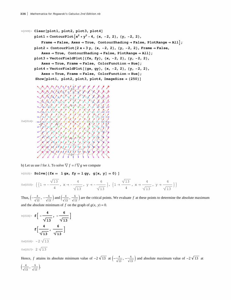
In[1509]:= Clearplot1, plot2, plot3, plot4plot1 ContourPlotx2 y2 4, x, 2, 2, y, 2, 2,

Frame False, Axes True, ContourShading False, PlotRange All;plot2 ContourPlot2 x 3 y, x, 2, 2, y, 2, 2, Frame False,

Axes True, ContourShading False, PlotRange All;plot3 VectorFieldPlotfx, fy, x, 2, 2, y, 2, 2,

Axes True, Frame False, ColorFunction Hue;plot4 VectorFieldPlotgx, gy, x, 2, 2, y, 2, 2,

Axes True, Frame False, ColorFunction Hue;Showplot1, plot2, plot3, plot4, ImageSize 250

Out[1514]=

b) Let us use l for l. To solve ! f = l ! g we compute

In[1515]:= Solvefx l gx, fy l gy, gx, y 0

Out[1515]= l 13

4, x

4

13, y

6

13, l

13

4, x

4

13, y

6

13

Thus, - 4

13, - 6

13 and 4

13, 6

13 are the critical points. We evaluate f at these points to determine the absolute maximum

and the absolute minimum of f on the graph of gx, y = 0.

In[1516]:= f 4

13,

6

13

f 4

13,

6

13

Out[1516]= 2 13

Out[1517]= 2 13

Hence, f attains its absolute minimum value of -2 13 at - 4

13, - 6

13 and absolute maximum value of -2 13 at

4

13,

6

13.


Here is a combined plot of the gradients of f (in black) and g (in red) at the critical points.

In[1518]:= Clearplot1, plot2, plot3, plot4, plot5, plot6plot1 ContourPlotgx, y, x, 3, 3, y, 3, 3,

Contours 0, Frame False, Axes True, ContourShading False;plot2 ListPlot 4

13,

6

13, 4

13,

6

13;

In[1521]:= plot3 GraphicsArrow

4

13,

6

13, 4

13,

6

13 fx, fy . x

4

13, y

6

13 ;

In[1522]:= plot4 Graphics

Arrow 4

13,

6

13 , 4

13,

6

13 fx, fy . x

4

13, y

6

13 ;

In[1523]:= plot5 GraphicsRed, Arrow 4

13,

6

13 ,

4

13,

6

13 gx, gy . x

4

13, y

6

13 ;

In[1524]:= plot6 GraphicsRed, Arrow

4

13,

6

13 , 4

13,

6

13 gx, gy . x

4

13, y

6

13 ;

In[1525]:= Showplot1, plot2, plot3, plot4, plot5, plot6,PlotRange All, AspectRatio Automatic, ImageSize 250

Out[1525]=

ü Exercises


1. Let f x, y = 4 x2 + 9 y2 and gx, y = x y - 4.a. Plot the level curves of f and g as well as their gradient vectors. b. Find the maximum and minimum values of f subject to gx, y = 0.

2. Find the maximum and minimum values of f x, y, z = x3 - 3 y2 + 4 z subject to the constraint gx, y, z = x + y z - 4 = 0.

3. Find the maximum area of a rectangle that can be inscribed in the ellipse x2

a2+

y2

b2= 1.

4. Find the maximum volume of a box that can be inscribed in the sphere x2 + y2 + z2 = 4.


Chapter 15 Multiple IntegrationUseful Tip: If you are reading the electronic version of this publication formatted as a Mathematica Notebook, then it is possibleto view 3-D plots generated by Mathematica from different perspectives. First, place your screen cursor over the plot. Then dragthe mouse while pressing down on the left mouse button to rotate the plot.

ü 15.1 Double Integral over a Rectangle


Integration can be generalized to functions of two or more variables. As the integral of a single-variable function defines area ofa plane region under the curve, it is natural to consider a double integral of a two-variable function that defines volume of a solidunder a surface. This definition can be made precise in terms of double Riemann sums where rectangular columns (as opposed torectangles) are used as building blocks to approximate volume (as opposed to area). The exact volume is then obtained as a limitwhere the number of columns increases without bound.

ü 15.1.1 Double Integrals and Riemann Sums

Let f x, y be a function of two variables defined on a rectangular domain R = a, bä c, d in R2. LetP = a = x0 < x1 < ... < xm = b, c = y0 < y1 < ... < yn = d be an arbitrary partition of R into a grid of m ÿn rectangles, where m and

n are integers. For each sub-rectangle Rij = xi-1, xiä y j-1, y j denote by DAij its area and choose an arbitrary base point

xij, yij œ Rij, where xij œ xi-1, xi and yij œ y j-1, y j. The product f xij, yijDAij represents the volume of the ij-rectangular

column situated between the surface and the xy-plane. We then define the double Riemann sum Sp of f x, y on R with respect

to P to be the total volume of all these columns:

SP =i=1

m

j=1

n

f xij, yijDAij

Define P to be the maximum dimension of all the sub-rectangles. The double integral of f x, y on the rectangle R is thendefined as the limit of SP as P Ø 0:

R

f x, y „A = limPØ0

i=1

m

j=1

n

f xij, yijDAij

If the limit exists regardless of the choice of partition and base points, then the double integral is said to exist. Otherwise, thedouble integral does not exist.

MIDPOINT RULE (Uniform Partitions): Let us consider uniform partitions P, where the points xi and y j are evenly

spaced, that is, xi = a + iD x, y j = b + jD y for i = 0, 1, ..., m and j = 0, 1, ..., n, and with Dx = b - a m and Dy = d - c n.

Then the corresponding double Riemann sum is

Sm,n =i=1

m

j=1

n

f xij, yijD xD y

Here is a subroutine called MDOUBLERSUM that calculates the double Riemann sum Sm,n of f x, y over a rectangle R for

uniform partitions using the center midpoint of each sub-rectangle as base point, that is, xij = xi-1 + xi 2 = a + i - 1 2D x and

yij = y j-1 + y j2 = c + j - 1 2D y.


In[1526]:= ClearfMDOUBLERSUMa_, b_, c_, d_, m_, n_ :

Sumfa i 1 2 b a m, c j 1 2 d c n b a m d c n,i, 1, m, j, 1, n

Example 15.1. Approximate the volume of the solid bounded below the surface f x = x2 + y2 and above the rectangleR = -1, 1ä -1, 1 on the xy-plane using a uniform partition with m = 10 and n = 10 and center midpoints as base points. Thenexperiment with larger values of m and n and conjecture an answer for the exact volume.

Solution: We calculate the approximate volume for m = 10 and n = 10 using the subroutine MDOUBLERSUM:

In[1528]:= fx_, y_ x^2 y^2;

MDOUBLERSUM1, 1, 1, 1, 10, 10

Out[1529]=66

25

In[1530]:= NOut[1530]= 2.64

In[1531]:= TableMDOUBLERSUM1, 1, 1, 1, 10 k, 10 k, k, 1, 10

Out[1531]= 6625

,133

50,1798

675,533

200,1666

625,3599

1350,3266

1225,2133

800,16198

6075,3333

1250

In[1532]:= NOut[1532]= 2.64, 2.66, 2.6637, 2.665, 2.6656, 2.66593, 2.66612, 2.66625, 2.66634, 2.6664It appears that the exact volume is 8/3. To prove this, we evaluate the double Riemann sum Sm,n in the limit as m, nØ¶:

In[1533]:= ClearS, m, n;Sm_, n_ SimplifyMDOUBLERSUM1, 1, 1, 1, m, n

Out[1534]=4

32

1

m2

1

n2

In[1535]:= LimitLimitSm, n, m Infinity, n Infinity

Out[1535]=8

3

To see this limiting process visually, evaluate the following subroutine, called DOUBLEMIDPT, which plots the surface of thefunction corresponding to the double integral along with the rectangular columns defined by the double Riemann sum considered

in the previous subroutine MDOUBLERSUM.


In[1536]:= Clearf;DOUBLEMIDPTf_, a_, b_, m_, c_, d_, n_ : Module

dx, dy, i, j, xstar, ystar, mrect, plot,dx Nb a m;xstar Tablea i dx, i, 0, m;dy Nd c n;ystar Tablec j dy, j, 0, n;mcolumn TableCuboidxstari, ystarj, 0,

xstari 1, ystarj 1, fxstari xstari 1 2,ystarj ystarj 1 2, i, 1, m, j, 1, n;

plot Plot3Dfx, y, x, a, b, y, c, d, Filling Bottom;Showplot, Graphics3Dmcolumn, ImageSize 300

In[1538]:= fx_, y_ : x2 y^2;

DOUBLEMIDPTf, 1, 1, 10, 1, 1, 10

Out[1539]=

Here is an animation that demonstrates how the volume of the rectangular columns approach that of the solid in the limit asm, nØ¶:





In[1540]:= AnimateDOUBLEMIDPTf, 1, 1, a, 1, 1, a , a, 5, 50, 5

Out[1540]=

a

-1.0

-0.5

0.0

0.5

1.0-1.0

-0.5

0.0

0.5

1.0

0.0

0.5

1.0

ü 15.1.2 Double Integrals and Iterated Integrals in Mathematica

The Mathematica command for evaluating double integrals is the same as that for evaluating integrals of a single-variablefunction, except that two limits of integration must be specified, one for each independent variable. Thus:

Integrate[f[x,y],{x,a,c},{y,c,d}] analytically evaluates the double integral Rf x, y „A over the rectangle R = a, bä c, d.

NIntegrate[f[x,y],{x,a,c},{y,c,d}] numerically evaluates the double integral Rf x, y „A over the rectangle R = a, bä c, d.

Iterated Integrals: In practice, one does not actually use the limit definition in terms of Riemann sums to evaluate double

integrals, but instead apply Fubini's Theorem to easily compute them in terms of iterated integrals:

Fubini's Theorem: (Rectangular Domains) If R = x, y : a § x § b, c § y § d, then

R

f x, y „A = a

b

c

d

f x, y „ y „ x = c

d

a

b

f x, y „ x „ y

Thus, Mathematica will naturally apply Fubini's Theorem whenever possible to analytically determine the answer. Depending onthe form of the double integral, Mathematica may resort to more sophisticated integration techniques, such as contour integration,which are beyond the scope of this text.

Example 15.2. Calculate the volume of the solid bounded below by the surface f x = x2 + y2 and above the rectangleR = -1, 1ä -1, 1.Solution: The volume of the solid is given by the double integral R

f x, y „A. To evaluate it, we use the Integrate command:


In[1541]:= fx_, y_ : x^2 y^2;

Integratefx, y, x, 1, 1, y, 1, 1

Out[1542]=8

3

This confirms the conjecture that we made in the previous example for the exact volume.

NOTE: Observe that we obtain the same answer by explicitly computing this double integral as an integrated integral as follows.Moreover, for rectangular domains, the order of integration does not matter.

In[1543]:= IntegrateIntegratefx, y, x, 1, 1, y, 1, 1IntegrateIntegratefx, y, y, 1, 1, x, 1, 1

Out[1543]=8

3

Out[1544]=8

3

Example 15.3. Compute the double integral Rx e-y2

„A on the rectangle R = 0, 1ä 0, 1.Solution: Observe that the Integrate command here gives us an answer in terms of the non-elementary error function Erf:

In[1545]:= Integratex E^y^2, x, 0, 1, y, 0, 1

Out[1545]=1

4 Erf1

This is because the function f x, y = x e-y2 has no elementary anti-derivative with respect to y due to the Gaussian factor e-y2

(bell curve). Thus, we instead use the NIntegrate Command to numerically approximate the double integral:

In[1546]:= NIntegratex E^y^2, x, 0, 1, y, 0, 1Out[1546]= 0.373412

ü Exercises

1. Consider the function f x, y = 16 - x2 - y2 defined over the rectangle R = 0, 2ä -1, 3.a. Use the subroutine MDOUBLERSUM to compute the double Riemann sum Sm,n of f x, y over R for m = 2 and n = 2.

b. Repeat part a) by generating a table of double Riemann sums for m = 10 k and n = 10 k where k = 1, 2, ..., 10. Make a

conjecture for the exact value of Rf x, y „A.

c. Find a formula for Sm,n in terms of m and n. Verify your conjecture in part b) by evaluating limm,nØ¶Sm,n.

d. Directly compute Rf x, y „A using the Integrate command.

2. Repeat Exercise 1 but with f x, y = 1 + x 1 + y 1 + x y defined over the rectangle R = 0, 1ä 0, 1.

3. Evaluate the double integral x4 + y4 „A over the rectangle R = -2, 1ä -1, 2 using both the Integrate and NInte-

grate commands. How do the two answers compare?

4. Calculate the volume of the solid lying under the surface z = e-yx + y2 and over the rectangle R = 0, 2ä 0, 3. Then make a

plot of this solid.


5. Repeat Exercise 4 but with z = sinx2 + y2 and rectangle R = - p , p ä - p , p .6. Evaluate the double integral R

f x, y „A where f x, y = x y cosx2 + y2 and R = -p, pä -p, p. Does your answer

make sense? Make a plot of the solid corresponding to this double integral to intuitively explain your answer. HINT: Considersymmetry.

7. Find the volume of solid bounded between the two hyperbolic paraboloids (saddles) z = 1 + x2 - y2 and z = 3 - x2 + y2 overthe rectangle R = -1, 1ä -1, 1.8. Find the volume of the solid bounded by the planes z = 2 x, z = -3 x + 2, y = 0, y = 1, and z = 0.

ü 15.2 Double Integral over More General Regions


For domains of integration that are non-rectangular but still simple, that is, bounded between two curves, Fubini's Theoremcontinues to hold. There are two types to consider:

Fubini's Theorem: (Simple Domains)

Type I (Vertically Simple): If D = x, y : a § x § b, ax § y § bx, then

D

f x, y „A = a

b

ax

bxf x, y „ y „ x

The corresponding Mathematica command is Integrate[f[x,y],{x,a,b},{y,a[x],b[x]}].

Type II (Horizontally Simple): If D = x, y : c § y § d, ay § x § by, then

D

f x, y „A = c

d

ay

byf x, y „ x „ y

The corresponding Mathematica command is Integrate[f[x,y],{y,c,d},{x,a[y],b[y]}].

Warning: Be careful not to reverse the order of integration prescribed for either type. For example, evaluating the command

Integrate[f[x,y],{y,a[x],b[x]},{x,a,b}] for Type I (x and y are reversed) will lead to incorrect results.

Example 15.4. Calculate the volume of the solid bounded below by the surface f x, y = 1 - x2 + y2 and above the domain Dbounded by x = 0, x = 1, y = x, and y = 1 + x2.

Solution: We observe that x = 0 and x = 1 represent the left and right boundaries, respectively, of D. Therefore, we plot thegraphs of the other two equations along the x-interval 0, 2 to visualize D (shaded in the following plot):


In[1547]:= Clearx, yplot1 Plotx, 1 x^2, x, 0, 1, Filling 1 2, ImageSize 250

Out[1548]=

Here is a plot of the corresponding solid situated over D:

In[1549]:= fx_, y_ 1 x^2 y^2;

plot3 Plot3Dfx, y, x, 0, 1, y, x, 1 x^2, Filling Bottom,ViewPoint 1, 1, 1, PlotRange 0, 4, ImageSize 250

Out[1550]=

To compute the volume of this solid given by Df x, y „A, we describe D as a vertically simple domain where 0 § x § 1 and

x § y § 1 + x2 and apply Fubini's Theorem to evaluate the corresponding iterated integral 0

1x

1+x2

f x, y „ y „ x (remember to use

the correct order of integration):

In[1551]:= Integratefx, y, x, 0, 1, y, x, 1 x2

Out[1551]=29

21

Example 15.5. Evaluate the double integral Dsin y2 „A, where D is the domain bounded by x = 0, y = 2, and y = x.

Solution: We first plot the graphs of x = 0, y = 2, and y = x to visualize the domain D:


In[1552]:= plot1 ContourPlotx 0, y 2, y x,x, 0.5, 2.5, y, 0.5, 2.5, ImageSize 250

Out[1552]=

-0.5 0.0 0.5 1.0 1.5 2.0 2.5

-0.5

0.0

0.5

1.0

1.5

2.0

2.5

It follows that D is the triangular region bounded by these graphs, which we shade in the following plot to make clear:

In[1553]:= plot2 Plotx, x, 0, 2, Filling 2;Showplot1, plot2, ImageSize 250

Out[1554]=

To compute the given double integral, we describe D as a horizontally simple domain, where 0 § y § 2 and 0 § x § y and apply

Fubini's Theorem to evaluate the corresponding iterated integral 0

20

ysiny2 „ x „ y (again, remember to use the correct order of

integration):

In[1555]:= IntegrateSiny^2, y, 0, 2, x, 0, yOut[1555]= Sin22In[1556]:= NOut[1556]= 0.826822

NOTE: It is also possible to view D as a vertically simple domain, where 0 § x § 2 and x § y § 2. The corresponding iterated


integral 02x

2siny2 „ y „ x gives the same answer, as it should by Fubini's Theorem:

In[1557]:= IntegrateSiny^2, x, 0, 2, y, x, 2Out[1557]= Sin22

Observe that it is actually impossible to evaluate this iterated integral by hand since there is no elementary formula for the anti-derivative of siny2 with respect to y. Thus, if necessary, Mathematica automatically switches the order of integration by

converting from one type to the other.

ü Exercises

In Exercises 1 through 4, evaluate the given iterated integrals and plot the solid corresponding to each one.

1. 0

10

x24 - x2 + y2 „ y „ x 2. 0

40

2-y2

x2 y „ x „ y

3. 0p0

sin qr2 cosq „ r „q 4. 0

10x y

1+x y„ y „ x

In Exercises 5 through 8, evaluate the given double integrals and plot the solid corresponding to each one.

5. Dx + y „A, D = x, y : 0 § x § 3, 0 § y § x

6. Dx + y „A, D = x, y : 0 § x § 1 - y2, 0 § y § 1

7. Dex+y „A, where D = x, y : x2 + y2 § 4

8. D

y

x+1„A, where D is the following shaded diamond region:

In Exercises 9 through 12, calculate the volume of the given solid S:9. S is bounded under the paraboloid z = 16 - x2 - y2 and above the region bounded between the line y = x and the parabolay = 6 - x2.

10. S is bounded under the right circular cone z = x2 + y2 and above the disk x2 + y2 § 1.

11. S is bounbed between the plane z = 5 + 2 x + 2 y and the paraboloid z = 12 - x2 - y2. HINT: Equate the two surfaces toobtain the equation of the domain.

12. S is bounded between the cylinders x2 + y2 = 1 and y2 + z2 = 1.

ü 15.3 Triple Integrals


Once the notion of a double integral is well established, it is straightforward to generalize it to triple (and even higher-order)integrals for functions of three variables defined over a solid region in space. Here is the definition of a triple integral in terms of


triple Riemann sums for a function f x, y, z defined on a box region B = x, y, z : a § x § b, c § y § d, p § z § q (refer to yourcalculus text for details):

B

f x, y „V = limPØ¶

i=1

m

j=1

n

k=1

p

f xijk , yijkDVijk

where the notation is analogous to that used for double integrals in Section 15.1 of this text. Of course, Fubini's Theorem alsogeneralizes to triple integrals:

Fubini's Theorem: (Box Domains) If B = x, y, z : a § x § b, c § y § d, p § z § q, then

B

f x, y „V = a

b

c

d

p

q

f x, y „ z „ y „ x

The corresponding Mathematica commands are:

Integrate[f[x,y,z],{x,a,c},{y,c,d},{z,e,f}] analytically evaluates the triple integral Bf x, y „V over the box

B = a, bä c, dä e, f . NIntegrate[f[x,y],{x,a,c},{y,c,d},{z,e,f}] numerically evaluates the triple integral B

f x, y „V over the rectangle

B = a, bä c, dä e, f . NOTE: For box domains, the order of integration does not matter so that it is possible to write five other versions of triple iteratedintegrals besides the one given in Fubini's Theorem.

Example 15.6. Calculate the triple integral Bx y z „V over the box B = 0, 1ä 2, 3ä 4, 5.

Solution: We use the Integrate command to calculate the given triple integral.

In[1558]:= Integratex y z, x, 0, 1, y, 2, 3, z, 4, 5

Out[1558]=45

8

Volume as Triple Integral: Recall that if a solid region W is bounded between two surfaces yx, y and fx, y, where both aredefined on the same domain D with yx, y § fx, y, then its volume V can be expressed by the triple integral

V = W

1 „V = Dyx,y

fx,y1 „ z „A

Example 15.7. Calculate the volume of the solid bounded between the surfaces z = 4 x2 + 4 y2 and z = 16 - 4 x2 - 4 y2 on therectangular domain -1, 1ä -1, 1.Solution: Here is a plot of the solid:


In[1559]:= Plot3D4 x^2 4 y^2, 16 4 x^2 4 y^2, x, 1, 1, y, 1, 1,Filling 1 8, 2 8, ImageSize 250, ImagePadding 15, 15, 15, 15

Out[1559]=

The volume of the solid is given by the triple iterated integral -11 -1

1 4 x2+4 y2

16-4 x2-4 y2

1 „ z „ y „ x:

In[1560]:= Integrate1, x, 0, 1, y, 1, 0, z, 4 x^2 4 y^2, 16 4 x^2 y^2

Out[1560]=35

3

ü Exercises

In Exercises 1 through 4, evaluate the given iterated integrals:

1. 0

10

x0

y2x + y + z „ z „ y „ x 2. 0

30

sin y0

y +zx y z „ x „ z „ y

3. 0p0

q0r cos q

r z2 „ z „ r „q 4. 01 x

1 01-y

z log1 + x y „ z „ y „ x

In Exercises 5 through 8, evaluate the given triple integrals:

5. Wx + y z „V , where W = x, y, z : 0 § x § 1, 0 § y § x , 0 § z § y2.

6. Wsin y „V , where W lies under the plane z = 1 + x + y and above the triangular region bounded by x = 0, x = 2, and

y = 3 x.

7. Wz „V , where W is bounded by the paraboloid z = 4 - x2 - y2 and z = 0.

8. Wf x, y, z „V , where f x, y, z = z2 and W is bounded between the cone z = x2 + y2 and z = 9.

9. The triple integral 0

1x21-x20

2-x-2 y„ z „ y „ x represents the volume of a solid S. Evaluate this integral. Then make a plot of S

and describe it.

10. Midpoint Rule for Triple Integrals:

a. Develop a subroutine called MTRIPLERSUM to compute the triple Riemann sum of the triple integral Bf x, y, z „V

over the box domain B = x, y, z : a § x § b, c § y § d, p § z § q for uniform partitions and using the center midpoint of each

sub-box as base point. HINT: Modify the subroutine MDOUBLERSUM in Section 15.1 of this text.

b. Use your subroutine MTRIPLESUM in part a) to compute the triple Riemann sum of Bx2 + y2 + z232 „V over the box

B = x, y, z : 0 § x § 1, 0 § y § 2, 0 § z § 3 by dividing B into 48 equal sub-boxes, that is, cubes having side length of 1/2.


c. Repeat part b) by dividing B into cubes having side length of 1/4 and more generally into cubes having side length of 1 2n forn sufficiently large in order to obtain an approximation accurate to 2 decimal places.

d. Verify your answer in part c) using Mathematica's NIntegrate command.

ü 15.4 Integration in Polar, Cylindrical, and Spherical Coordinates


ü 15.4.1 Double Integrals in Polar Coordinates

The following Change of Variables Formula converts a double integral in rectangular coordinates to one in polar coordinates:

Change of Variables Formula (Polar Coordinates):

I. Polar Rectangles: If R = r, q : q1 § q § q2, r1 § r § r2, then

R

f x, y „A = q1

q2

r1

r2

f r cos q, r sin q r „ r „q

II. Polar Regions: If D = r, q : q1 § q § q2, aq § r § bq, then

D

f x, y „A = q1

q2

aq

bqf r cos q, r sin q r „ r „q

Example 15.8. Calculate the volume of the solid region bounded by the paraboloid f x = 4 - x2 - y2 and the xy-plane usingpolar coordinates.

Solution: We first plot the paraboloid:

In[1561]:= fx_, y_ 4 x^2 y^2

Plot3Dfx, y, x, 2, 2, y, 2, 2, PlotRange 0, 4, ImageSize 250Out[1561]= 4 x2 y2

Out[1562]=

The circular domain D can be easily described in polar coordinates by the polar rectangle R = r, q : 0 § r § 2, 0 § q § 2 p.Thus, the volume of the solid is given by the corresponding double integral 0

2 p0

2f r cos q, r sin q r „ r „q in polar coordinates:


In[1563]:= Clearr, ;Integrater fr Cos, r Sin, r, 0, 2, , 0, 2 Pi

Out[1564]= 8

Observe that here f x, y simplifies nicely in polar coordinates:

In[1565]:= fr Cos, r SinSimplify

Out[1565]= 4 r2 Cos2 r2 Sin2Out[1566]= 4 r2

NOTE: Evaluating the same double integral in rectangular coordinates by hand would be quite tedious. This is not a problemwith Mathematica, however:

In[1567]:= Integratefx, y, x, 2, 2, y, Sqrt4 x^2, Sqrt4 x^2Out[1567]= 8

ü 15.4.2 Triple Integrals in Cylindrical Coordinates

The following Change of Variables Formula converts a triple integral in rectangular coordinates to one in cylindrical coordinates:

Change of Variables Formula (Cylindrical Coordinates): If a solid region W is described by q1 § q § q2, aq § r § bq, andz1r, q § z § z2r, q, then

W

f x, y, z „V = q1

q2

aq

bq

z1r,q

z2r,qf r cos q, r sin q, z r „ z „ r „q

Example 15.9. Use cylindrical coordinates to calculate the triple integral Wz „V , where W is the solid region bounded above

by the plane z = 8 - x - y, below by the paraboloid z = 4 - x2 - y2, and inside the cylinder x2 + y2 = 4.

Solution: Since W lies inside the cylinder x2 + y2 = 4, this implies that it has a circular base on the xy-plane given by the sameequation, which can be described in polar coordinates by 0 § q § 2 p and 0 § r § 2. Here is a plot of all three surfaces (plane,paraboloid, and cylinder):


In[1568]:= plotplane Plot3D8 x y, x, 2, 2, y, 2, 2;plotparaboloid Plot3D4 x^2 y^2, x, 2, 2, y, 2, 2;plotcylinder

ParametricPlot3D2 Cos, 2 Sin, z, , 0, 2 , z, 0, 12;Showplotplane, plotparaboloid, plotcylinder, PlotRange All, ImageSize 250

Out[1571]=

Since W is bounded in z by 4 - x2 - y2 § z § 8 - x - y, or in cylindrical coordinates, 4 - r cos q - r sin q § z § 4 - r2, it followsthat the given triple integral transforms to

0

2 p0

24-r2

4-r cos q-r sin qz r „ z „ r „q

Evaluating this integral in Mathematica yields the answer

In[1572]:= Integratez r, , 0, 2 , r, 0, 2,z, 4 r Cos r Sin, 8 r Cos r Sin

Out[1572]= 96

ü 15.4.3 Triple Integrals in Spherical Coordinates

The following Change of Variables Formula converts a triple integral in rectangular coordinates to one in spherical coordinates:

Change of Variables Formula (Spherical Coordinates): If a solid region W is described by q1 § q § q2, f1 § f § f2, andr1q, f § r § r2q, f, then

W

f x, y, z „V = q1

q2

f1

f2

r1q,f

r2q,ff r cos q sin f, r sin q sin f, r cos f r2 sinf „ r „f „q

Example 15.10. Use spherical coordinates to calculate the volume of the solid W lying inside the sphere x2 + y2 + z2 = z and

above the cone z = x2 + y2 .

Solution: In spherical coordinates, the equation of the sphere is given by

r 2 = r cos f

or equivalently, r = cos f. Similarly, the equation of the cone transforms to

r cos f = r cos q sin f2 + r sin q sin f2 = r sin f


It follows that cos f = sin f, or f = p 4. Therefore, the cone makes an angle of 45 degrees with respect to the z-axis, as shown inthe following plot along with the top half of the sphere:

In[1573]:= Clearplotcone ParametricPlot3D Cos SinPi 4, Sin SinPi 4, CosPi 4,

, 0, 2 Pi, , 0, Sqrt2 2;plotsphere ParametricPlot3DCos Cos Sin,

Cos Sin Sin, Cos Cos, , 0, 2 Pi, , 0, Pi 4;Showplotcone, plotsphere, PlotRange All, ViewPoint 1, 1, 1 4,ImageSize 250

Out[1576]=

It is now clear that the solid W is described by 0 § q § 2 p, 0 § f § p 4, and 0 § r § cos f. Thus, its volume is given by the tripleintegral

0

2 p

0

p4

0

cos f

r2 sin f „ r „f „q

which in Mathematica evaluates to

In[1577]:= Integrate^2 Sin, , 0, 2 Pi, , 0, Pi 4, , 0, Cos

Out[1577]=

8

ü Exercises

In Exercises 1 through 4, evaluate the given double integral by converting to polar coordinates:

1. -11

- 1-x2

1-x2 1 - x2 - y2 „ y „ x 2. 020

4-x2

e-x2+y2 „ y „ x

3. Dx log y „A, where D is the annulus (donut-shaped region) with inner radius 1 and outer radius 3.

4. Darctan

y

x„A, where D is the region inside the cardioid r = 1 + cos t.

5. Use polar coordinates to calculate the volume of the solid that lies below the paraboloid z = x2 + y2 and inside the cylinderx2 + y2 = 2 y.


6. Evaluate the triple integral 0

20

4-x2 0

4-x2-y2 x2 + y2 „ z „ y „ x by converting to cylindrical coordinates.

7. Use cylindrical coordinates to calculate the triple integral Wx2 + y 2 „V , where W is the solid bounded between the two

paraboloids z = x2 + y2 and z = 8 - x2 - y2.

8. Evaluate the triple integral -2

2 - 4-x2

4-x2 x2+y2

4-x2-y2 x2 + y2 + z2 „ z „ y „ x by converting to spherical coordinates.

9. The solid defined by the spherical equation r = sin f is called the torus.a. Plot the torus.b. Calculate the volume of the torus.

10. Ice-Cream Cone: A solid W in the shape of an ice-cream cone is bounded below by the cylinder z = x2 + y2 and above by

the sphere x2 + y2 + z2 = 8. Plot W and determine its volume.

ü 15.5 Applications of Multiple Integrals


Mass as Double Integral: Consider a lamina (thin plate) D in R2 with continous mass density rx, y. Then the mass of D isgiven by the double integral

M = Drx, y „A

where the domain of integration is given by the region that describes the lamina D.

Example 15.11. Calculate the mass of the lamina D bounded between the parabola y = x2 and y = 4 with density rx, y = y.

Solution: Here is a plot of the lamina D (shaded):

In[1578]:= Plotx^2, 4, x, 2, 2, ImageSize 250, Filling 2 1

Out[1578]=

We can view D as a Type I region described by -2 § x § 2 and x2 § y § 4. Thus. the mass of the lamina is given by the doubleintegral:

In[1579]:= Integratey, x, 2, 2, y, x^2, 4

Out[1579]=128

5


NOTE: Mass of a lamina can also be interpreted as the volune of the solid bounded by its density function over D as shown in thefollowing plot:

In[1580]:= Plot3Dy, x, 2, 2, y, 0, 4, RegionFunction 1^2 2 4 &,Filling Bottom, Mesh None, ImageSize 250

Out[1580]=

Example 15.12. Suppose a circular metal plate D, bounded by x2 + y2 = 9, has electrical charge density

rx, y = 9 - x2 - y2 . Calculate the total charge of the plate.

Solution: Here is a plot of the metal plate D (shaded):

In[1581]:= Integratey, x, 2, 2, y, x^2, 4

Out[1581]=128

5

In[1582]:= PlotSqrt9 x^2, Sqrt9 x^2, x, 3, 3,ImageSize 250, Filling 2 1, AspectRatio 1

Out[1582]=

We shall calculate the total charge of the plate using polar coordinates, which will simplify the corresponding double integral.

Since rr, q = 9 - r2 and D is a simple polar region described by r = 3, the total charge is


In[1583]:= IntegrateSqrt9 r^2 r, r, 0, 3, theta, 0, 2 PiOut[1583]= 18

Mass as Triple Integral: We can extend the notion of mass to a solid region W in R3. Suppose W is bounded between twosurfaces z = yx, y and z = fx, y, where both are defined on the same domain D with yx, y § fx, y, and has densityrx, y, z. Then the mass of W can be expressed by the triple integral

M = Wrx, y, z „V =

Dyx,y

fx,yrx, y, z „ z „A

Example 15.13. Calculate the mass of the solid region W bounded between the planes z = 1 - x - y and z = 1 + x + y andsituated over the triangular domain D bounded by x = 0, y = 0, and y = 1 - x. Assume the density of W is given byrx, y, z = 1 + x2 + y2.

Solution: Here is a plot of the solid region W:

In[1584]:= Plot3D1 x y, 1 x y, x, 0, 1, y, 0, 1 x, ViewPoint 1, 1, 1,Filling 1 1, 2 1, Ticks Automatic, Automatic, 1, 2,ImageSize 250, ImagePadding 15, 15, 15, 15

Out[1584]=

The mass of the solid is given by the triple iterated integral 010

1-x1-x-y1+x+y1 + x2 + y2 „ z „ y „ x:

In[1585]:= Integrate1 x^2 y^2, x, 0, 1, y, 0, 1 x, z, 1 x y, 1 x y

Out[1585]=14

15

Center of Mass: Given a lamina D in R2, its center of mass xCM, yCM (or balance point) is defined as the ratio of its moments(with respect to the coordinate axes) to its mass:

xCM =My

M, yCM =

Mx

M

where the moments My and Mx are defined by

My =1

A

Dx rx, y „A, Mx =

1

A

Dy rx, y „A


NOTE: In case the lamina has uniform density, that is, rx, y = 1, then the center of mass is the same as the centroid whosecoordinates represent averages of the coordinates over the lamina.

Center of mass (and centroid) can be naturally extended to solid objects in R3. Refer to your textbook for further details.

Example 15.14. Calculate the mass of the solid region W bounded between the planes z = 1 - x - y and z = 1 + x + y andsituated over the triangular domain D bounded by x = 0, y = 0, and y = 1 - x. Assume the density of W is given byrx, y, z = 1 + x2 + y2.

ü Exercises

In Exercises 1 and 2, find the mass of the given lamina D.1. D is bounded between y = sin p x and y = 0 along the interval 0, 1 and has density rx, y = x1 - x .2. D is bounded by the lines y = x + 1, y = -2 x - 2, and x = 1 and has density rx, y = 1 + y2 .

3. Find the center of mass of the lamina D in Exercises 1 and 2.

4. Find the centroid of the lamina in Exercises 1 and 2. Compare the centroid of each lamina with its center of mass.

In Exercises 5 and 6, find the mass of the given solidi object W.5. W is the interior of the tetrahedron enclosed by the planes x = 0, y = 0, z = 0, and z = 1 - x - y and has densityrx, y, z = 1 - z.

6. W is the ice-cream cone bounded below by the cylinder z = x2 + y2 and above by the sphere x2 + y2 + z2 = 8 and has

density rx, y, z = z2.

7. Find the center of mass of the tetrahedron in Exercises 5 and 6. Refer to your textbook for appropriate formulas.

8. Find the centroid of the tetrahedron in Exercises 5 and 6. Compare this with its center of mass. Refer to your textbook forappropriate formulas.

ü 15.6 Change of Variables


A change of variables is often useful for simplifying integrals of a single variable (commonly referred to as u-substitution):

a

b

f x „ x = c

d

f gu g ' u „u

where x = gu, a = gc, and b = gd. This substitution formula allows one to transformation an integral in the variable x to onein a new variable u. Observe that the interval c, d is mapped to interval a, b under the function g.

This technique can be extended to double integrals of the form Df x, y „ x „ y, where a change of variables is described by a

transformation Gu, v = x, y, which maps a region D0 in the uv-coordinate plane to the region D in the xy-coordinate plane.

The following Change of Variables Formula converts a double integral from the xy-coordinate system to a new coordinate systemdefined by u and v:

Change of Variables Formula (Coordinate Transformation): If Gu, v = xu, v, yu, v is a C1-mapping from D0 to D, then

D

f x, y „ x „ y = D0

f xu, v, yu, v ∑ x, y∑ u, v „u „v


where ∑x,y∑u,v , referred to as the Jacobian of G and also denoted by Jac(G), is given by

JacG = ∑ x, y∑ u, v =

∑x

∑u

∑x

∑v∑y

∑u

∑y

∑v

=∑ x

∑u

∑ y

∑v-∑ x

∑v

∑ y

∑u

The Jacobian relates the area of any infinitesimal region inside D0 with the corresponding region inside D =GD0. In fact, if Gis a linear map, then Jac(G) is constant and is equal in magnitude to the ratio of the areas of D to that of D0:

Jacobian of a Linear Map: If Gu, v = A u + C v, B u + D v is a linear mapping from D0 to D, then Jac(G) is constant withvalue

JacG = A C

B D= A D - B C

Moreover,

AreaD = JacG AreaD0Refer to your textbook for a detailed discussion of transformations of plane regions.

Example 15.12. Make an appropriate changes of variables to calculate the double integral Dx y „A, where D is the region

bounded by the curves x y = 1, x y = 2, x y2 = 1, and x y2 = 2.

Solution: Here is a plot of the shaded region D bounded by the four given curves:

In[1586]:= plot1 ContourPlotx y 1, x y 2, x y^2 1, x y^2 2,x, 0, 5, y, 0, 5, AspectRatio Automatic, ImageSize 250;

plot2 ContourPlot1, x, 0, 5, y, 0, 5, AspectRatio Automatic,RegionFunction Functionx, y, 1 x y 2 && 1 x y^2 2,ImageSize 250, PlotPoints 100;

Showplot1,plot2

Out[1588]=

0 1 2 3 4 5

0

1

2

3

4

5

Observe that D is rather complicated. Since D can be described by the inequalities 1 < x y < 2 and 1 < x y2 < 2, we make thenatural change of variables u = x y and v = x y2, which transforms D to a simple square region D0 in the uv-plane bounded by


u = 1, u = 2, v = 1, and v = 2:

In[1589]:= ContourPlot1, u, 0, 3, v, 0, 3, ImageSize 250,RegionFunction Functionu, v, 1 u 2 && 1 v 2

Out[1589]=

0.0 0.5 1.0 1.5 2.0 2.5 3.0

0.0

0.5

1.0

1.5

2.0

2.5

3.0

To find the formula for our transformation Gu, v = xu, v, yu, v that maps D0 to D, we solve for x and y in terms of u and v:

In[1590]:= Clearsol, x, y, u, vsol Solveu x y, v x y^2, x, y

Out[1591]= x u2

v, y

v

u

It follows that Gu, v = u2 v, v u and the corresponding Jacobian is

In[1592]:= x sol1, 1, 2y sol1, 2, 2Jac Dx, u Dy, v Dx, v Dy, u

Out[1592]=u2

v

Out[1593]=v

u

Out[1594]=1

v

Thus, the given integral transforms to Dx y „A = D0

u

v„A = 1

21

2 u

v„v „u with value

In[1595]:= Integrateu v, u, 1, 2, v, 1, 2

Out[1595]=3 Log2

2

ü Exercises

1. Consider the transformation Gu, v = 2 u + v, u - 3 v.a. Set D =GD0 where D0 = 0 § u § 1, 0 § v § 2. Make a plot of D and describe its shape.


b. Compute JacG.c. Compare the area of D with that of D0. How does this relate to JacG?

2. Compute the area of the ellipse x2

4+

y2

9= 1 by viewing it as a transformation of the unit circle u2 + v2 = 1 under a linear map

Gu, v = xu, v, yu, v and using the area relationship described by Jac(G).

3. Evaluate the integral Dx y „A, where D is the region in the first quadrant bounded by the equations y = x, y = 4 x, x y = 1,

and x y = 4. HINT: Consider the change of variables u = x y and v = y.

4. Evaluate the integral Dx + y x - y „A, where D is the parallelogram bounded by the lines x - y = 1, x - y = 3,

2 x + y = 0, and 2 x + y = 2. HINT: Consider the change of variables u = x - y and v = 2 x + y.

5. Evaluate the integral D

y

x„A, where D is the region bounded by the circles x2 + y2 = 1, x2 + y2 = 4 and lines y = x, y = 3 x.

HINT: Consider the change of variables u = x2 + y2 and v = y x.


Chapter 16 Line and Surface IntegralsUseful Tip: If you are reading the electronic version of this publication formatted as a Mathematica Notebook, then it is possibleto view 3-D plots generated by Mathematica from different perspectives. First, place your screen cursor over the plot. Then dragthe mouse while pressing down on the left mouse button to rotate the plot.

ü 16.1 Vector Fields


Let F1, F2, and F3 be functions of x, y, and z. The vector-valued function

Fx, y, z = F1x, y, z, F2x, y, z, F3x, y, zis called a vector field. We have already encountered a vector field in the form of the gradient of a function. Other useful exam-ples of vector fields are the gravitational force, the velocity of fluid, magnetic fields, and electric fields.

We use the Mathematica commands VectorFieldPlot and VectorFieldPlot3D to plot the graphs of vector fields. However,

before using these commands, it is advisable to load the VectorFieldPlots package. This is done by evaluating

In[1596]:= Needs"VectorFieldPlots`"Example 16.1. Draw the following vector fields.a) Fx, y = sin y, cos x b) F x, y, z = y, x + z, 2 x - y Solution:a)

In[1597]:= ClearF, x, y, zFx_, y_ Siny, Cosx

Out[1598]= Siny, CosxIn[1599]:= VectorFieldPlotFx, y, x, 5, 5, y, 4, 4, ImageSize 250

Out[1599]=

Here is another display of the preceding vector field with some options specified.


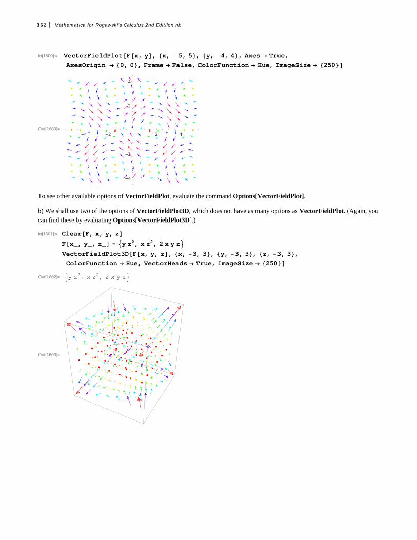
In[1600]:= VectorFieldPlotFx, y, x, 5, 5, y, 4, 4, Axes True,

AxesOrigin 0, 0, Frame False, ColorFunction Hue, ImageSize 250

Out[1600]=-4 -2 2 4

-4

-2

2

4

To see other available options of VectorFieldPlot, evaluate the command Options[VectorFieldPlot].

b) We shall use two of the options of VectorFieldPlot3D, which does not have as many options as VectorFieldPlot. (Again, you

can find these by evaluating Options[VectorFieldPlot3D].)

In[1601]:= ClearF, x, y, zFx_, y_, z_ y z2, x z2, 2 x y zVectorFieldPlot3DFx, y, z, x, 3, 3, y, 3, 3, z, 3, 3,ColorFunction Hue, VectorHeads True, ImageSize 250

Out[1602]= y z2, x z2, 2 x y z

Out[1603]=


Example 16.2. Draw the unit radial vector fields:

a) Fx, y = x

x2+y2,

y

x2+y2 b) F x, y, z = x

x2+y2+z2,

y

x2+y2+z2, z

x2+y2+z2

Solution: For convenience, we define both vector fields to be 0 at the origin. We shall use the If command to do so.

a)

In[1604]:= ClearF, x, yFx_, y_ Ifx2 y2 0,

x, yx2 y2

, 0, 0

VectorFieldPlotFx, y, x, 3, 3, y, 3, 3, ImageSize 250

Out[1605]= Ifx2 y2 0,x, yx2 y2

, 0, 0

Out[1606]=


b)

In[1607]:= ClearF, x, y, zFx_, y_, z_ Ifx2 y2 z2 0,

x, y, zx2 y2 z2

, 0, 0, 0

VectorFieldPlot3DFx, y, z, x, 3, 3, y, 3, 3, z, 3, 3,ColorFunction Hue, VectorHeads True, ImageSize 250

Out[1608]= Ifx2 y2 z2 0,x, y, zx2 y2 z2

, 0, 0, 0

Out[1609]=

ü Exercises

In Exercise 1 through 4, draw the given vector fields.

1. Fx, y = y2 - 2 xy, xy + 6 x2 2. F x, y, z = sin x, cos y , xz 3. Fx, y = - y

x2+y2, x

x2+y2 4, F x, y, z = x + cos xz, y sin xy, xz cos yz

In Exerices 5 and 6, calculate and plot the gradient vector field for each of the following functions.5. f x, y = lnx + y2 6. f x, y, z = sin x cos z y

ü 16.2 Line Integrals


Suppose C is a smooth curve in space whose parametric equations are given by

x = xt, y = yt, z = ztwhere a § t § b. Let C1, C2, C3, .... , CN be a partition of the curve C with arc length Ds1, Ds2, Ds3, ... , DsN and letP1, P2, P3, ... , PN be points on the subarcs.


If f x, y, z is a function that is continuous on the curve C, then the line integral of f is defined by

Cf x, y, z „ s = limDsiØ0 i=1

N f PiDsi

NOTE: If c t = xt, yt, zt is the vector equation of the curve C, then it can be shown (refer to your calculus textbook) that

Cf x, y, z „ s = a

bf ct c ' t „ t

In addition, if Fx, y, z = F1, F2, F3 is a vector field that is continuous on C, then the line integral of F over C is given by

CFx, y, z ◊„ s = C

F ◊ T „ s = a

bF ct ◊c ' t „ t

where T is the unit vector T = c' tc' t and F ◊ T is the dot product of F and T.

Example 16.3. Find Cf x, y, z „ s, where f x, y, z = x y + z2 and C is given by x = t, y = t2, and z = t3, for 0 § t § 1.

Solution:

In[1610]:= Clearx, y, z, t, f, cfx_, y_, z_ x 2 y x z

xt_ t

yt_ t2

zt_ t3

ct_ xt, yt, ztOut[1611]= x2 y x z

Out[1612]= t

Out[1613]= t2

Out[1614]= t3

Out[1615]= t, t2, t3


In[1616]:= 0

1

fxt, yt, zt Normc't t

Out[1616]= 1

76545 722 5

2 114 84 987 134 2 5 532 14 EllipticEArcSin 3 3

2 2 5 ,

2 5

2 5 266 70 EllipticEArcSin 3 3

2 2 5 , 2 5

2 5

415 14 EllipticFArcSin 3 3

2 2 5 , 2 5

2 5

266 70 EllipticFArcSin 3 3

2 2 5 , 2 5

2 5

Here is a numerical approximation of the preceding line integral.

In[1617]:= NIntegratefxt, yt, zt Normc't, t, 0, 1Out[1617]= 1.16521

Example 16.4. Find CFx, y, z ◊„ s, where Fx, y, z = x z, z y2, y x2 and the curve C is given by x = 2 t, y = sin t, and

z = cos t, 0 § t § 2 p.

Solution:


In[1618]:= Clearx, y, z, t, f, cFx_, y_, z_ x z, z y2, y x2xt_ 2 t

yt_ Sintzt_ Costct_ xt, yt, zt

Out[1619]= x z, y2 z, x2 yOut[1620]= 2 t

Out[1621]= SintOut[1622]= CostOut[1623]= 2 t, Sint, Cost

In[1624]:= 0

2 Pi

Fxt, yt, zt.c't t

Out[1624]=9

416 3

3

In[1625]:= NOut[1625]= 158.298

ü Exercises

1. Find Cf x, y, z „ s, where:

a. f x, y, z = x y2 - 4 zy and C is given by x = 2 t, y = t23, and z = 1 - 3 t2, for 0 § t § 1.

b. f x, y, z = yz

x and C is given by x = ln t, y = t2, and z = 3 t, for 3 § t § 5.

2. Find CFx, y ◊„ s, where:

a. Fx, y = e3 x-2 y, e2 x+3 y and C is given by x = 2 t, y = sin t, 0 § t § p

b. Fx, y = x2, yx + y2 and C is the unit circle center at the origin.

3. Find CFx, y, z ◊„ s, where:

a. Fx, y, z = xyz, -xz, xy and C is given by x = t, y = 2 t2, z = 3 t 0 § t § 1

b. Fx, y, z = xy3, z + x2, z3 and C is the line segment joining -1, 2, -1 and 1, 3, 4.

ü 16.3 Conservative Vector Fields


Let Fx, y, z = F1, F2, F3 be a vector field. Let C1 and C2 be any two different curves with the same initial point P and end

point Q. We say that the vector field F is path independent if

C1Fx, y, z ◊„ s = C2

Fx, y, z ◊„ s


A vector field that is path independent is called conservative.

NOTE 1: A vector field F is conservative if

C

Fx, y, z ◊„ s = 0

for every closed curve C.

NOTE 2: If F = !u is the gradient of a function u = ux, y, z, then we say that u is the potential of F. Moreover, if the endpoints of C are P and Q, we have

C

Fx, y, z ◊„ s = uP - uQ

In particular, if the curve is closed, that is, if P =Q, then

C

Fx, y, z ◊„ s = 0

Therefore, gradient is conservative. The converse of this statement is true if its domain is an open connected domain.

NOTE 3: Let F = F1, F2. If F =!u = ∑ u

∑ x, ∑ u

∑ y, then F1 =

∑ u

∑ x and F2 =

∑ u

∑ y. Taking the partial derivative of F1with respect to y

and that of F2 with respect to x and using the fact that ∑2 u

∑ x ∑ y= ∑2 u

∑ y ∑ x, we see that F1 and F2 must satisfy

∑ F1

∑ y=

∑ F2

∑ x

This equation is used to check if a vector field is conservative. In that case, we solve F1 =∑ u

∑ x for u by integrating with respect to

x and then use the equation F2 =∑ u

∑ y to find the constant of integration. Here is an example.

Example 16.5. Show that the vector function F = 3 x2 - 2 xy + 2, 6 y2 - x2 + 3 is conservative and find its potential.

Solution: Here, F1 = x y2 and F2 = x2 y. We now compare ∑ F1

∑ y and

∑ F2

∑ x to verify if F is conservative.

In[1626]:= Clearx, y, F1, F2F1x_, y_ 3 x2 2 x y 2

F2x_, y_ 6 y2 x2 3

Out[1627]= 2 3 x2 2 x y

Out[1628]= 3 x2 6 y2

In[1629]:= DF1x, y, yDF2x, y, x

Out[1629]= 2 x

Out[1630]= 2 x

Thus, the vector field is conservative. To find its potential u, we integrate F1 =∑ u

∑ x with respect to x to get


In[1631]:= Clearh, uu IntegrateF1x, y, x hy

Out[1632]= 2 x x3 x2 y hyNote that the addition of hy is necessary because the constant of integration may depend on y. We now solve the equation

F2 =∑ u

∑ y for h ' y.

In[1633]:= Clearsolsol SolveDu, y F2x, y, h'y

Out[1634]= hy 3 1 2 y2This means that h ' y = 3 1 + 2 y2.In[1635]:= Integratesol1, 1, 2, yOut[1635]= 3 y 2 y3

Hence, hy = 3 y + 2 y2 and so ux, y = 2 x + x3 - x2 y + 3 y + 2 y3 is the potential of F.

NOTE 4: Let F = F1, F2, F3. If F =!u = ∑ u

∑ x,∑ u

∑ y,∑ u

∑ z, then F1 =

∑ u

∑ x, F2 =

∑ u

∑ y and F3 =

∑ u

∑ z. Taking the partial derivative of

F1with respect to y and that of F2 with respect to x and using the fact that ∑2 u

∑x ∑y= ∑2 u

∑y ∑x, we see that F1 and F2 must satisfy

∑ F1

∑ y=

∑ F2

∑ x

Taking the partial derivative of F1with respect to z and that of F3 with respect to x and using the fact that ∑2 u

∑x ∑z= ∑2 u

∑z ∑x, we see that

F1 and F3 must satisfy

∑ F1

∑ z=

∑ F3

∑ x

The preceding two equations can be used to check if a vector field is conservative. If this the case, we solve F1 =∑ u

∑ x for u by

integrating with respect to x and then use F2 =∑ u

∑ y to find the constant of integration. We show this by the following example.

Example 16.6. Show that the vector function F = yz + yz cos xy , xz + xz cos xy , xy + sin xy is conservative and find itspotential.

Solution: Here, F1 = y z + y z cos x y , F2 = x z + x z cos x y, and F3 = x y + sinx y .

In[1636]:= Clearx, y, F1, F2, F3F1x_, y_, z_ y z y z Cosx yF2x_, y_, z_ x z x z Cosx yF3x_, y_, z_ x y Sinx y

Out[1637]= y z y z Cosx yOut[1638]= x z x z Cosx yOut[1639]= x y Sinx y

We now compare ∑ F1

∑ y and

∑ F2

∑ x:


In[1640]:= DF1x, y, z, yDF2x, y, z, x

Out[1640]= z z Cosx y x y z Sinx yOut[1641]= z z Cosx y x y z Sinx y

Next, we compare ∑ F1

∑ z and

∑ F2

∑ x:

In[1642]:= DF1x, y, z, zDF3x, y, z, x

Out[1642]= y y Cosx yOut[1643]= y y Cosx y

Thus, the vector field is conservative. To find its potential u, we integrate F1 =∑ u

∑ x with repsetct to x to get

In[1644]:= Clearu, hu IntegrateF1x, y, z, x hy, z

Out[1645]= x y z hy, z z Sinx yNote that the addition of hy, z is necessary because the constant of intgeration can depend on y and z. We now solve the

equation F2 =∑ u

∑ y for ∑ h

∑ y.

In[1646]:= Clearsolsol SolveDu, y F2x, y, z, y hy, z

Out[1647]= h1,0y, z 0

This means that ∑ h

∑ y= 0 and hence h is a function of z only. Next, we solve the equation F3 =

∑ u

∑ z for ∑ h

∑ z.

In[1648]:= Clearsol2sol2 SolveDu, z F3x, y, z, z hy, z

Out[1649]= h0,1y, z 0

Hence, ∑ h

∑ z= 0 and we can take h = 0. Therefore, u = x y z + z sin x y is the potential for the vector field F.

ü Exercises

1. Show that the vector field F = y3 - 3 x2 y, 3 xy2 - x3 is conservative and find its potential.

2. Show that the vector field F = y z +2 xy

z, xz + x2

z, xy -

x2 y

z2 is conservative and find its potential.

3. Determine whether the vector field F = x2, yx + ez, y ez is conservative. If it is, find its potential.

ü 16.4 Parametrized Surfaces and Surface Integrals



A parametrized surface is a surface whose points are given in the form

Gu, v = xu, v, yu, v, zu, vwhere u and v (called parameters) are independent variables used to describe a domain D (called the parameter domain).

The command for plotting parametrized surfaces is ParametricPlot3D. This command has been discussed in Section 14.1.2 ofthis text.


Example 16.7. Plot the parametrized surface defined by Gu, v = cos u sin v, 4 sin u cos v, cos v over the domainD = u, v 0 § u § 2 p, 0 § v § 2 p.Solution:

In[1650]:= ParametricPlot3D Cosu Sinv, 4 Sinu Cosv, Cosv,u, 0, 2 Pi, v, 0, 2 Pi, ImageSize 250

Out[1650]=

Example 16.8. Plot the parametrized surface defined by Gu, v = u cos v, u sin v, 1 - u2 over the domain

D = u, v 0 § u § 1, 0 § v § 2 p.Solution:

In[1651]:= ParametricPlot3Du Cosv , u Sinv , 1 u2, u, 0, 1,v, 0, 2 Pi, ColorFunction "BlueGreenYellow", ImageSize 250,ImagePadding 15, 15, 15, 15

Out[1651]=

NOTE: On a parametrized surface Gu, v = xu, v, yu, v, zu, v, if we fix one of the variables, we get a curve on thesurface. The plot following shows the curves corresponding to u = 3 4 (latitude) and v = 5 p 3 (longitude).


In[1652]:= Clearplot1, plot2, plot3plot1 ParametricPlot3Du Cosv , u Sinv , 1 u2,

u, 0, 1, v, 0, 2 Pi, ColorFunction "BlueGreenYellow";plot2 ParametricPlot3D 3 4 Cosv , 3 4 Sinv , 7 16,

v, 0, 2 Pi, PlotStyle Thickness0.01, Red;plot3 ParametricPlot3D u Cos5 Pi 3 , u Sin5 Pi 3 , 1 u2,

u, 0, 1, PlotStyle Thickness0.01, Blue;Showplot1, plot2, plot3, PlotRange All, ImageSize 250,ImagePadding 15, 15, 15, 15

Out[1656]=

Let P =Gu0, v0 be a point on the parametrized surface S. For fixed v = v0, the tangent vector to the curve Gu, v0 at u0, v0 isgiven by

Tu =∑G

∑uu0, v0

while the tangent vector for Gu0, v corresponding to a fixed u = u0 is given by

Tv =∑G

∑vu0, v0

These two vectors are tangent to the surface S. Thus, the normal vector n to the tangent plane at Gu0, v0 is given by

n P = n u0, v0 = TuμTv

Example 16.9. Consider the parametrized surface Gu, v = u cos v, u sin v, 1 - v2.a) Find Tu, Tv, and n.b) Find the equation of the tangent plane at 1 2, 5 p 3.c) Plot the tangent plane and surface.

Solution: Let us define G as a function of u and v in Mathematica.

In[1657]:= ClearG, u, vGu_, v_ u Cosv, u Sinv, 1 u2

Out[1658]= u Cosv, u Sinv, 1 u2a) We use Tu for Tu and Tv for Tv. We evaluate these as functions of u and v.


In[1659]:= ClearTu, Tv, nTuu_, v_ DGu, v, uTvu_, v_ DGu, v, vnu_, v_ CrossTuu, v, Tvu, v

Out[1660]= Cosv, Sinv, 2 uOut[1661]= u Sinv, u Cosv, 0Out[1662]= 2 u2 Cosv, 2 u2 Sinv, u Cosv2 u Sinv2b) The normal vector to the tangent plane at 1 2, 5 p 3 is

In[1663]:= Clearnormalnormal n1 2, 5 Pi 3

Out[1664]= 14,

3

4,1

2

The tangent plane passes through the point

In[1665]:= Clearpointpoint G1 2, 5 Pi 3

Out[1666]= 14,

3

4,3

4

Thus, the equation of the tangent plane is given by

In[1667]:= Cleartplanetplane normal.x, y, z point 0

Out[1668]=1

41

4 x

1

43

3

4 y

1

23

4 z 0

which simplifies to

In[1669]:= SimplifytplaneOut[1669]= 2 x 4 z 5 2 3 y

c) Here is the plot of the surface and the tangent plane. Observe that we have used ColorFunction and ColorFunctionScalingoptions.


In[1670]:= Clearplot1, plot2plot1 ParametricPlot3DGu, v,

u, 0, 1, v, 0, 2 Pi, ColorFunction "BlueGreenYellow";plot2 ContourPlot3D2 x 4 z 5 2 3 y, x, 3, 3, y, 3, 3,

z, 4, 4, ColorFunction Functionx, y, z, HueModz, 1,ColorFunctionScaling False;

Showplot1, plot2, ImageSize 250, ImagePadding 15, 15, 15, 15

Out[1673]=

NOTE: The area AS of a parametrized surface S: Gu, v = xu, v, yu, v, zu, v, where u, v œ D, is given by

AS = D nu, v „u „v

If f x, y, z is continuous at all points of S, then the surface area of f over S is given by

Sf x, y, z „S = D

f Gu, v nu, v „u „v

Example 16.10. Show the following:a) The area of the cylinder of height h and radius r is 2 p rh.b) The area of the sphere of radius r is 4 p r2.

Solution: a) A parametric equation of the cylinder of height h and radius r can be given by

x = r cos v, y = r sin v, and z = u, where 0 § v § 2 p , 0 § u § h

Thus, the cylinder is given by Gu, v = r cos u, r sin u, v. In[1674]:= Clear G, u, v, r

Gu_, v_ r Cosv, r Sinv, uOut[1675]= r Cosv, r Sinv, uHere is a plot of the cylinder with r = 3 and h = 5:


In[1676]:= r 3; h 5;

ParametricPlot3DGu, v, u, 0, h, v, 0, 2 Pi

Out[1677]=

To compute the surface area of the cylinder, we need to compute its normal vector.

In[1678]:= ClearTu, Tv, n, r, hTuu_, v_ DGu, v, u;Tvu_, v_ DGu, v, v;nu_, v_ CrossTuu, v, Tvu, v

Out[1681]= r Cosv, r Sinv, 0Here is a plot of the cylinder with its normal vector for r = 3 and h = 5:


In[1682]:= r 3; h 5;

Clearplot1, plot2plot1 ParametricPlot3DGu, v, u, 0, h, v, 0, 2 Pi;plot2 VectorFieldPlot3Dnu, v, u, 0, h,

v, 2 Pi, 2 Pi, z, 3, 3, VectorHeads True, PlotPoints 15;Showplot1, plot2, ImageSize 250Clearr, h

Out[1686]=

The surface area is

In[1688]:= SArea 0

h

0

2 Pi

Normnu, v v uOut[1688]= 2 h AbsrSince r > 0, r = r and hence the preceding output is 2 p r h .

b) A parametric equation of the sphere of radius r is

x = r cos u sin v, y = r sin u sin v, z = r cos v

where 0 § u § 2 p and 0 § v § p. Thus, the sphere is given by Gu, v = r cos u sin v, r sin u sin v, r cos v. In[1689]:= Clear G, u, v, r

Gu_, v_ r Cosu Sinv, r Sinu Sinv, r CosvOut[1690]= r Cosu Sinv, r Sinu Sinv, r CosvHere is a plot of the sphere with r = 3.


In[1691]:= r 3;

ParametricPlot3DGu, v, u, 0, 2 Pi, v, 0, Pi, ImageSize 250

Out[1692]=

To compute the surface area of the sphere, we need to compute its normal vector.

In[1693]:= ClearTu, Tv, n, rTuu_, v_ DGu, v, u;Tvu_, v_ DGu, v, v;nu_, v_ CrossTuu, v, Tvu, v

Out[1696]= r2 Cosu Sinv2, r2 Sinu Sinv2,r2 Cosu2 Cosv Sinv r2 Cosv Sinu2 Sinv

Here is a plot of the sphere with its normal vector for r = 3.


In[1697]:= r 3; h 5;

Clearplot1, plot2plot1 ParametricPlot3DGu, v, u, 0, 2 Pi, v, 0, h;plot2 VectorFieldPlot3Dnu, v, u, 2 Pi, 2 Pi,

v, 0, h, z, 3, 3, VectorHeads True, PlotPoints 10;Showplot1, plot2, ImageSize 250Clearr, h

Out[1701]=

The surface area is

In[1703]:= SArea 0

Pi

0

2 Pi

Normnu, v u vOut[1703]= 4 r ConjugaterFor a real number r, the conjugate of r is r and hence the preceding output is 4 p r2.

Example 16.11. Consider the parametrized surface S defined by Gu, v = u cos v, u sin v, v, where 0 § u § 1, 0 § v § 2 p.a) Find the surface area of S.

b) Evaluate Sxyz „S.

Solution:a)

In[1704]:= Clear G, u, vGu_, v_ u Cosv, u Sinv, v

Out[1705]= u Cosv, u Sinv, v


In[1706]:= ClearTu, Tv, nTuu_, v_ DGu, v, uTvu_, v_ DGu, v, vnu_, v_ CrossTuu, v, Tvu, v

Out[1707]= Cosv, Sinv, 0Out[1708]= u Sinv, u Cosv, 1Out[1709]= Sinv, Cosv, u Cosv2 u Sinv2 The surface area AS is given by

In[1710]:= SArea 0

1

0

2 Pi

Normnu, v v u

Out[1710]= 2 ArcSinh1which is approximately equal to

In[1711]:= NOut[1711]= 7.2118

b) We define f :

In[1712]:= Clearffx_, y_, z_ x y z

Out[1713]= x y z

The surface integral of f is

In[1714]:= 0

1

0

2 Pi

fGu, v1, Gu, v2, Gu, v3 Normnu, v v u

Out[1714]= 1

16 3 2 ArcSinh1

Or numerically,

In[1715]:= NOut[1715]= 0.659983

ü Exercises

1. Plot the parametrized surface Gu, v = eu sin v, eu cos v, v over the domain D = u, v -1 § u § 1, 0 § v § 2 p. 2. Plot the parametrized surface Gu, v = 3 sin u cos v, sin u sin v, cos v + 3 cos u over the domain D = u, v 0 § u § 2 p, 0 § v § 2 p.3. Consider the parametrized surface Gu, v = e-u cos v, eu sin v, eu cos v.a. Find Tu, Tv, and n.b. Find the equation of the tangent plane at 0, p 2.c. Plot the tangent plane and surface.


4. Consider the parametrized surface S: Gu, v = u - v , 3 u + v, u2 - 2 u v + 6 v2, where 0 § u § 1, 0 § v § 1.

a. Find the surface area of S. (Use NIntegrate for faster integration.)

b. Evaluate S3 x + 2 y2 - z2 „S.

ü 16.5 Surface Integrals of Vector Fields


An orientation of a surface S is a continuously varying choice of the unit normal vector enP at each point of the surface. Thus,en is given by either

enP = nPnP or enP = - nP

nP

If Fx, y, z is continuous at all points of a parametrized surface S, then the surface integral of F over S is given by

SF ÿ„S = S

F ÿen „S

where en is the unit normal determined by an orientation. The surface integral of F is also called the flux of F across S.

The surface integral of F over a parametrized surface S given by Gu, v = xu, v, yu, v, zu, v, where u, v œ D, is given by

SF ÿ„S = S

F ÿen „S = DFGu, v ◊nu, v „u „v

Example 16.12. Find SF ◊„S, where Fx, y, z = x z, z , y x and S is given by Gu, v = u - v2, u v, u2 - v, 0 § u § 2, and

1 § v § 3.

Solution:

In[1716]:= ClearF, G, x, y, z, u, vFx_, y_, z_ x z, z, y xGu_, v_ u v2, u v, u2 v

Out[1717]= x z, z, x yOut[1718]= u v2, u v, u2 vIn[1719]:= ClearTu, Tv, n

Tuu_, v_ DGu, v, uTvu_, v_ DGu, v, vnu_, v_ CrossTuu, v, Tvu, v

Out[1720]= 1, v, 2 uOut[1721]= 2 v, u, 1Out[1722]= 2 u2 v, 1 4 u v, u 2 v2

In[1723]:= Flux 0

2

1

3

FGu, v1, Gu, v2, Gu, v3 .nu, v v u

Out[1723]= 6928

15


Example 16.13. Find SF ◊„S, where Fx, y, z = x2, z2 , y + x2 and S is the upper hemisphere x2 + y2 + z2 = 4 with

outward normal orientation.

Solution: First, we find the parametric equation of the cylinder. This can be given by x = 2 cos u sin v, y = 2 sin u sin v, andz = 2 cos v, where 0 § u § 2 p and 0 § v § p 2.

For the hemisphere to have the outward orientation, we note that n = TvμTu. With this in mind we compute the flux of F acrossS through the following steps.

In[1724]:= ClearF, G, x, y, z, u, vFx_, y_, z_ x2, z2, x2 y z3Gu_, v_ 2 Cosu Sinv , 2 Sinu Sinv , Cosv

Out[1725]= x2, z2, x2 y z3Out[1726]= 2 Cosu Sinv, 2 Sinu Sinv, CosvIn[1727]:= ClearTu, Tv, n

Tuu_, v_ DGu, v, uTvu_, v_ DGu, v, vnu_, v_ CrossTvu, v, Tuu, v

Out[1728]= 2 Sinu Sinv, 2 Cosu Sinv, 0Out[1729]= 2 Cosu Cosv, 2 Cosv Sinu, SinvOut[1730]= 2 Cosu Sinv2, 2 Sinu Sinv2, 4 Cosu2 Cosv Sinv 4 Cosv Sinu2 Sinv

In[1731]:= Flux 0

Pi20

2 Pi

FGu, v1, Gu, v2, Gu, v3 .nu, v u v

Out[1731]=28

5

ü Exercises

1. Find SF ◊„S, where Fx, y, z = ez, z, y x and S is given by Gu, v = u v, u - v, u, 0 § u § 2, and -1 § v § 1, and

oriented by n = TuμTv.

2. Find SF ÿ„S, where Fx, y, z = z, x , y and S is the portion of the ellipsoid x2

16+

y2

9+ z2

4= 1 for which x § 0, y § 0, and

z § 0 with outward normal orientation.

3. Let S be given by Gu, v = 1 + v cosu

2 cos u, 1 + v cos

u

2 sin u , v sin

u

2, 0 § u § 2 p, and

-1

2§ v § 1

2.

a. Plot the surface S. (S is an example of a Mobius strip.)b. Find the surface area of S.

c. Evaluate Sx2 + 2 y2 + 3 z2 „S.

d. Find the intersection points of S and the xy-plane.

e. For each of the points on the intersection of S and the xy-plane, find the normal vector n.

f. Show that n varies continuously but that n2 p, 0 = -nu, 0. (This shows that S is not orientable and hence it is impossible to integrate a vector field over S.)


Chapter 17 Fundamental Theorems of Vector AnalysisUseful Tip: If you are reading the electronic version of this publication formatted as a Mathematica Notebook, then it is possibleto view 3-D plots generated by Mathematica from different perspectives. First, place your screen cursor over the plot. Then dragthe mouse while pressing down on the left mouse button to rotate the plot.

NOTE: In order to perform the operations of curl and divergence on vector fields discussed in this section using Mathematica, it

is necessary to first load the VectorAnalysis package:

In[1732]:= Needs"VectorAnalysis`"The Fundamental Theorem of Calculus for functions of a single variable states that the integral of a function f x over an intervala, b (domain) can be calculated as the difference of its anti-derivative Fx at the endpoints (boundary) of the interval:

a

b

f x „ x = Fb - Fa

This integral relationship between domain and boundary can be generalized to vector fields involving the operations of curl anddivergence and is made precise by three theorems that will be discussed in this chapter: Green's Theorem, Stoke's Theorem, andDivergence Theorem.

ü 17.1 Green's Theorem


Let Fx, y = Px, y, Qx, y a vector field continuous on an oriented curve C. Recall that the line integral of F along C isdenoted by

CFx, y, z ◊„ s = C

P „ x +Q „ y

If c t = xt, yt, zt is the vector equation of the curve C, then

CP „ x +Q „ y = a

bPxt, yt d x

d t+Qxt, yt d y

d t d t

The following is a generalization of the Fundamental Theorem of Calculus to two dimensions, which relates a double integralover a region with a corresponding line integral along its boundary.

Green's Theorem: If C is a simple closed curve oriented counterclockwise and D is the region enclosed, and if P and Q aredifferentiable and have continuous first partial derivatives, then

CP „ x +Q „ y = D

∑Q

∑ x- ∑ P

∑ y „A

Refer to your textbook for a detailed discussion and proof of Green's Theorem.

Example 17.1. Compute the line integral Ce2 x+y „ x + e-y „ y, where C is the boundary of the square with vertices 0, 0, 1, 0,

1, 1, 1, 0 oriented counterclockwise.

Solution: We will use Green's Theorem. Thus, we need to verify that the hypotheses of Green's Theorem hold. To this end, we


define the function P and Q and compute their partial derivatives.

In[1733]:= Clearx, y, P, QPx_, y_ E2 xy

Qx_, y_ Ey

Out[1734]= 2 xy

Out[1735]= y

In[1736]:= DPx, y, xDPx, y, yDQx, y, xDQx, y, y

Out[1736]= 2 2 xy

Out[1737]= 2 xy

Out[1738]= 0

Out[1739]= y

The partial derivatives are continuous inside the square and the curve is oriented counterclockwise. Thus, the hypotheses ofGreen's Theorem are satisfied. Note that the region D enclosed by C is given by 0 § x § 1 and 0 § y § 1.

In[1740]:= 0

1

0

1

DQx, y, x DPx, y, y y x

Out[1740]= 1

21 2 1

In[1741]:= NOut[1741]= 5.4891

NOTE: If we were to solve this using the definition of line integral as discussed in Chapter 16 of this text, we would then need toconsider four pieces of parametrization of C and then sum the four integrals. Toward this end, let us use C1 for the lower edge,C2 for the right edge, C3 for the top edge, and C4 for the left edge of the square. Here are the parametrizations followed by theirline integrals.


In[1742]:= Clearx1, x2, x3, x4, y1, y2, y3, y4, t, F, c1, c2, c3, c4Fx_, y_ Px, y, Qx, y x1t_ t

y1t_ 0

c1t_ x1t, y1t

x2t_ 1

y2t_ t

c2t_ x2t, y2t

x3t_ 1 t

y3t_ 1

c3t_ x3t, y3t

x4t_ 0

y4t_ 1 t

c4t_ x4t, y4tOut[1743]= 2 xy, yOut[1744]= t

Out[1745]= 0

Out[1746]= t, 0Out[1747]= 1

Out[1748]= t

Out[1749]= 1, tOut[1750]= 1 t

Out[1751]= 1

Out[1752]= 1 t, 1Out[1753]= 0

Out[1754]= 1 t

Out[1755]= 0, 1 t

In[1756]:= 0

1

Fx1t, y1t.c1't t 0

1

Fx2t, y2t.c2't t

0

1

Fx3t, y3t.c3't t 0

1

Fx4t, y4t.c4't t

Out[1756]= 1 1

1

1

21 2 1

2 1 2

In[1757]:= NOut[1757]= 5.4891


ü Exercises

In Exercises 1 through 4, use Green's Theorem to evaluate the given line integral.

1. Cy2 sin x „ x + x y „ y, where C is the boundary of the triangle with vertices 0, 0, 1, 0, 1, 1, oriented counterclockwise.

2. C2 x2 y „ x + x3 „ y, where C is the circle x2 + y2 = 4, oriented counterclockwise.

3. Cx2 + y2 „ x + y ex „ y, where C is the boundary of the region bounded between the parabola y = 5 - x2 and the line

y = 2 x - 3, oriented clockwise.

4. Cx

x2+y2„ x -

y

x2+y2„ y, where C is the boundary of the quarter-annulus situated between the circles x2 + y2 = 1 and x2 + y2 = 9

in the first quadrant (see plot below), oriented counterclockwise.

5. Let Fx, y = 2 x y + y3, x2 + 3 x y + 2 y. Use Green's Theorem to demonstrate that the line integral CFx, y, z ◊„ s = 0 for

every simple closed curve C. What kind of a vector field do we call F?

ü 17.2 Stokes's Theorem


Let Fx, y, z = F1, F2, F3 be a vector field. The curl of F, denoted by curlF or ! μF, is defined by

curlF =! μF =

i j k∑

∑x

∑

∑y

∑

∑z

F1 F2 F3

= ∑F3

∑y-

∑F2

∑z,∑F1

∑z-

∑F3

∑x,∑F2

∑x-

∑F1

∑y

Here, we are using the del or symbol ! (nabla) to denote the vector operator ! = ∑

∑x, ∑

∑y, ∑

∑z.

The Mathematica command for computing the curl of a vector field F is Curl[F,coordsys], where coordsys is the coordinatesystem of the vector field. This is demonstrated in the next example.

The following is a generalization of the Fundamental Theorem of Calculus three dimensions, which relates a surface integralinvolving curl with a corresponding line integral along its boundary.

Stokes's Theorem: If Fx, y, z a vector field with continuous partial derivatives and if S is an oriented surface S with boundary∑S, then

∑SF ÿ„S = S

curlF ◊„S

If S is closed, then it has no boundary and hence both integrals are equal to 0.

NOTE: Recall that if the surface S is given by Gu, v = xu, v, yu, v, zu, v, where u, v œ D, then ScurlF ÿ„S is given

by

ScurlF ◊„S = D

curlF Gu, v ◊nu, v „u „v

Refer to your textbook for a detailed discussion and proof of Stokes's Theorem.


Example 17.2. Find the curl of the vector field Fx, y, z = x sin y z, ex y z , y x2.Solution: We use the Curl command:

In[1758]:= ClearF, F1, F2, F3, x, y, zF1 x Siny zF2 Exy zF3 x 2 y

F F1, F2, F3Out[1759]= x Siny zOut[1760]= xy z

Out[1761]= x2 y

Out[1762]= x Siny z, xy z, x2 yIn[1763]:= CurlF, Cartesianx, y, z

Out[1763]= xy x2, 2 x y x y Cosy z, xy zy

x z Cosy z

NOTE: We obtain the same answer for the curl of F using the explicit formula:

In[1764]:= curl y F3 zF2, zF1 xF3, xF2 yF1


x z Cosy z

Or equivalently,

In[1765]:= CurlF DF3, y DF2, z, DF3, x DF1, z, DF2, x DF1, y


x z Cosy z

Example 17.3. Let f x, y, z be a function of three variables with continuous first and second partial derivatives and let F =! f

be the gradient of f . Find the curl of the vector field F.

Solution:

In[1766]:= Clearf, F1, F2, F3, x, y, zF1 Dfx, y, z, xF2 Dfx, y, z, yF3 Dfx, y, z, zF F1, F2, F3

Out[1767]= f1,0,0x, y, zOut[1768]= f0,1,0x, y, zOut[1769]= f0,0,1x, y, zOut[1770]= f1,0,0x, y, z, f0,1,0x, y, z, f0,0,1x, y, z


Then the curl of F is

In[1771]:= CurlF, Cartesianx, y, zOut[1771]= 0, 0, 0To see why the curl is zero, let us examine each partial derivative used in computing the curl of F.

In[1772]:= DF3, yDF2, z

Out[1772]= f0,1,1x, y, zOut[1773]= f0,1,1x, y, zNOTE: Here, f 0,1,1x, y, z stands for the second partial derivative fyz. Thus, the two partial derivatives that appear in the x-

component of the curl of F are equal and hence their difference is zero. Similarly, we have

In[1774]:= DF3, xDF1, z

Out[1774]= f1,0,1x, y, zOut[1775]= f1,0,1x, y, zand

In[1776]:= DF2, xDF1, y

Out[1776]= f1,1,0x, y, zOut[1777]= f1,1,0x, y, zExample 17.4. Compute ∑S

F ÿ„S, where Fx, y, z = x y z, z + 3 x - 3 y , y 2 x and S is the upper hemisphere of radius 4.

Solution: Note that ∑S is a circle of radius 4 lying on the xy-plane. Hence, ∑S can be parametrized by the curvect = xt, yt, zt where

x = 4 cos t, y = 4 sin t, z = 0, where 0 § t § 2 p

We then use this parametrization to evaluate the line integral ∑SF ÿ„S =0

2 pFxt, yt, zt ÿc ' t „ t:


In[1778]:= ClearF, x, y, z, t, c, curlFFx_, y_, z_ x y z, z 3 x 3 y, y2 xxt_ 4 Costyt_ 4 Sintzt_ 0

ct_ xt, yt, ztOut[1779]= x y z, 3 x 3 y z, x y2Out[1780]= 4 CostOut[1781]= 4 SintOut[1782]= 0

Out[1783]= 4 Cost, 4 Sint, 0

In[1784]:= 0

2 Pi

Fxt, yt, zt.c't tOut[1784]= 48

Next, we use Stokes's Theorem to obtain the same answer via the corresponding surface integral. The parametrization of theupper hemisphere of radius 4 is given by Su, v = xu, v, yu, v, zu, v, where

x = 4 cos u sin v, y = 4 sin u sin v, and z = 4 cos v, where 0 § u § 2 p, 0 § v § p 2

We now compute the normal of the upper hemisphere:

In[1785]:= ClearS, u, v, Tu, Tv, nSu_, v_ : 4 Cosu Sinv, 4 Sinu Sinv, 4 Cosv Tuu_, v_ : DSu, v, uTvu_, v_ : DSu, v, vnu_, v_ CrossTvu, v, Tuu, v

Out[1789]= 16 Cosu Sinv2, 16 Sinu Sinv2,16 Cosu2 Cosv Sinv 16 Cosv Sinu2 Sinv

The curl of F is

In[1790]:= curlFx_, y_, z_ CurlFx, y, z, Cartesianx, y, zOut[1790]= 1 2 x y, x y y2, 3 x zThus, the surface integral is given by

In[1791]:= 0

Pi20

2 Pi

curlFSu, v1, Su, v2, Su, v3 .nu, v u vOut[1791]= 48

This answer agrees with the one obtained using the line integral definition.

Example 17.5. Find the flux of the curl of the vector field Fx, y, z = x2, z2 , y + x2 across S, where S is the part of the cone

z2 = x2 + y2 for which 1 § z § 4 with outward normal orientation.


Solution: First, we will need the following parametric equations to describe the cone S: x = u cos v , y = u sin v, and z = u, where0 § v § 2 p and 1 § u § 4.

For the cone to have outward orientation, we set n = TvμTu (right-hand rule) since Tv points in the horizontal direction aroundthe cone and Tu points in the direction along the length of the cone.

In[1792]:= ClearF, S, u, v, Tu, Tv, nFx_, y_, z_ x2 y2, x z2, 0Su_, v_ : u Cosv , u Sinv , u Tuu_, v_ : DSu, v, uTvu_, v_ : DSu, v, vnu_, v_ CrossTvu, v, Tuu, v

Out[1793]= x2 y2, x z2, 0Out[1797]= u Cosv, u Sinv, u Cosv2 u Sinv2 We now compute the flux of curl F across S through the following steps.

In[1798]:= curlFx_, y_, z_ CurlFx, y, z, Cartesianx, y, zOut[1798]= 2 z, 0, 1 2 y

In[1799]:= Flux 1

4

0

2 Pi

curlFSu, v1, Su, v2, Su, v3.nu, v v uOut[1799]= 15

ü Exercises

NOTE: In order to perform the curl operation in Mathematica, it is necessary to first load the VectorAnalysis package. Seeinstructions given at the beginning of this chapter.

In Exercises 1 and 2, find the curl of the given vector field.

1. Fx, y, z = ln x2 + y2 + z2, x z , ex sin y z2. Fx, y, z = - x

x2+y2+z232 , -y

x2+y2+z232 , - z

x2+y2+z232

In Exercises 3 and 4, verify Stokes's Theorem for the given vector field F and surface S.

3. Fx, y, z = x3 e - 3 x y + z3, 2 z3 - x z2 + y4, 6 y + 2 z3 x2 and S is the part of the paraboloid z = x2 + y2 for which z § 9 and

with outward normal orientation.4. Fx, y, z = x y z, x y, x + y + z and S is the elliptical region in the plane y + z = 2 whose boundary is the intersection of the plane with the cylinder x2 + y2 = 1 and with upward normal orientation.

In Exercises 5 and 6, use Stokes's Theorem to compute the flux of the curl of the vector field F across the surface S.

5. Fx, y, z = tanx y z, ey-x z, secy2 x and S is the upper hemisphere of radius 4.

6. Fx, y, z = x2 z, x y2, z2 and S consists of the top and four sides of the cube (excluding the bottom) with vertices at 0, 0, 0, 1, 0, 0, 0, 1, 0, 1, 1, 0, 0, 0, 1, 1, 0, 1, 0, 1, 1, 1, 1, 1.

ü 17.3 Divergence Theorem

Students should read Section 17.3 of Rogawski's Calculus [1] for a detailed discussion of the material presented in this


g psection.

Let Fx, y, z = F1, F2, F3 be a vector field. The divergence of F, denoted by divF or ! ◊ F, is defined by

divF = ! ◊ F =∑F1

∑x+

∑F2

∑ y+

∑F3

∑z

where ! = ∑

∑x, ∑

∑y, ∑

∑z.

The Mathematica command for computing the divergence of a vector field F is Div[F,coordsys], where coordsys is the coordi-nate system of the vector field. This is demonstrated in the next example.

The following is another generalization of the Fundamental Theorem of Calculus three dimensions, which relates a triple integralof a solid object involving divergence with a corresponding surface integral along its boundary.

Divergence Theorem: Let W be a region in R3 whose boundary ∑W is a piecewise smooth surface, oriented so that the normalvectors to ∑W point outside of W , and Fx, y, z be a vector field with continuous partial derivatives whose domain contains W .Then

∑WF ◊„S = W

divF „V

Refer to your textbook for a detailed discussion and proof of the Divergence Theorem.

Example 17.8. Find the divergence of the vector field Fx, y, z = x sin yz, ex y z , yx2.Solution:

In[1800]:= ClearF1, F2, F3, x, y, zF1 x Siny zF2 Exy zF3 x 2 y

F F1, F2, F3Out[1801]= x Siny zOut[1802]= xy z

Out[1803]= x2 y

Out[1804]= x Siny z, xy z, x2 yThen the divergence of F is

In[1805]:= DivF, Cartesianx, y, z

Out[1805]= xy x z

y2 Siny z

NOTE: Again we obtain the same answer for the divergence of F using the explicit formula:

In[1806]:= DF1, x DF2, y DF3, z

Out[1806]= xy x z

y2 Siny z

Example 17.9. Find SF ◊„S, where Fx, y, z = x , y2, y + z and S = ∑W is the boundary of the region W contained in the


cylinder x2 + y2 = 4 between the plane z = x and z = 8.

Solution: If S is the boundary of the solid W , then W is given by

W = x, y, z : -2 § x § 2, - 4 - x2 § y § 4 - x2 , x § z § 8In[1807]:= ClearF, divF, x, y, z

Fx_, y_, z_ x, y2, y zdivF DivFx, y, z, Cartesianx, y, z

Out[1808]= x, y2, y zOut[1809]= 2 2 y

By the Divergence Theorem, we see that SF ÿ„S is given by

In[1810]:= 2

2

4x2

4x2

x

8

divF z y x

Out[1810]= 64

ü Exercises

NOTE: In order to perform the divergence operation in Mathematica, it is necessary to first load the VectorAnalysis package.See instructions given at the beginning of this chapter.

In Exercises 1 and 2, find the divergence of the given vector field F.

1. Fx, y, z = x y z, x2 + y2 + z2, x y + y z + x z2. Fx, y, z = ex y cos z, ey z sin z, z2In Exercises 3 and 4, verify the Divergence Theorem for the given vector field F and solid region W.

3. Fx, y, z = x2 y, y2 z, z2 x and W = x, y, z : x2 + y2 + z2 < 1 is the unit ball.

4. Fx, y, z = ex cos y, ex sin y, x y z and W is the region bounded by the paraboloid z = x2 + y2 and z = 4.

In Exercises 5 and 6, use the Divergence Theorem to calculate the flux of the vector field F across the surface S.

5. Fx, y, z = x ez , y2, y + z x and S is tetrahedron bounded by the plane 3 x + 4 y + 5 z = 15 and the coordinate planes in the

first octant.

6. Fx, y, z = x y z, x2 + y2 + z2, x y + y z + x z and S is the unit cube with vertices at 0, 0, 0, 1, 0, 0, 0, 1, 0, 1, 1, 0, 0, 0, 1, 1, 0, 1, 0, 1, 1, 1, 1, 1.


Appendices - Quick Reference Guides

ü A. Common Mathematical Operations - Traditional Notation versus Mathematica Notation

The following list demonstrates how to translate common mathematical operations described using traditional notation intoMathematica notation. In many instances Mathematica's palettes (see Section 1.5) will allow the user to input commands usingtraditional notation without having to convert to Mathematica notation.

Operation Traditional Notation Mathematica Notation

Define a function f x = x2 f = x^2 or

f x_ = x^2 or

f x_ := x^2 (delayed assignment)

Evaluate a function f 1 f . x -> 1 or f 1

Square root f x Sqrt[ f x]Absolution value f x Abs[ f x]Limit lim

xØaf x Limit f x, x -> a

Derivative f ' x f ' x or D f x, xSecond derivative f '' x f '' x or D f x, x, 2Indefinite integral f x „ x Integrate f x, x

Definite integral (Exact) ab

f x „ x Integrate f x, x, a, b

Definite integrate (Approximate) a

bf x „ x NIntegrate f x, x, a, b

Pi p Pi or p (from palette menu)

Euler number e E or ‰ (from palette menu)

Imaginary number i I or Â (from palette menu)

Infinity ¶ Infinity or ¶ (from palette menu)

Sine function sin x SinxInverse sine function arcsin x or sin-1 x ArcSinxExponential function ex E^x or Expx or ‰x (from palette menu)

Natural logarithm (base e) ln x LogxLogarithm (base a) log a x Logx, aDefine i-th element of a sequence xi = a xi = a or xi = a (from palette menu)


ü B. Useful Commands for Plotting, Solving, and Manipulating Mathematical Expressions

Mathematica Command Description

Plot f x, x, a, b Plot a function f x on the interval a, bPlot3D f x, y, x, a, b, y, c, d Plot a two-variable function f x, y on a, bμ c, dParametricPlotxt, yt, t, a, b Plot parametric equations x = f t, y = gt on a, bPolarPlot f q, q, a, b Plot polar function r = f q on a, bContourPlot f x, y, x, a, b, y, c, d Plot contour of f x, y on a, bμ c, dContourPlotFx, y == 0, x, a, b, y, c, d Plot implicit function Fx, y = 0 on a, bμ c, dSolve f x == gx, x Solve an equation f x = gx for x

DSolveFx, y, y ' xä 0, yx, x Solve a differential equation Fx, y, y ' x = 0 for yxwith initial value y ' 0 = a

Part[expr,i] or expr[[i]] Refer to i-th element of list expr

N[expr] or N[expr,n] (n-digit precision) Numerical approximation of a quantity expr

Simplifyexpr Reduce an expression expr to most simple

ü C. Useful Editing and Programming Commands

Mathematica Command Description

SHIFT+ENTER Evaluates input

% Refers to previous output

%% Refers to second previous output

%k or Out[k] Refers to output line k

In[k] Refers to input line k

CTRL+L Reproduces the previous input

CTRL+SHIFT+L Reproduces the previous output

?Plot Lists all Mathematica commands containing the expression Plot (or any other specified command)

(* expr *) Insert comment expr (unevaluated)

If[test,expr,else] Evaluate expr if test is true; otherwise, evaluate else

Do[expr,{i,min,max,step}] Evaluate expr through loop i running from min to max with increment step

While[test, expr] Evaluate expr while test is true; otherwise stop


ü D. Formatting Cells in a Notebook

Mathematica organizes a notebook in terms of data boxes called cells. The size of a cell is indicated by the corresponding size ofthe right bracket symbol attached to the right hand margin of each cell. A new cell can always be created by moving the cursorto any position between cells and begin typing. To edit a cell, just move the cursor to the desired position within that cell.

Each cell can be formatted to perform a specified function. By default, a new cell is always formatted as an input cell, which areused to evaluate Mathematica expressions. Mathematica outputs are contained within output cells, naturally. Other cell formatsincluded title, section, subsection, text, formula, etc. The format of a cell is indicated by the left-most box on the toolbar. Tochange its format, first highlight the cell by clicking on the right bracket symbol attached to it. Then click on the indicator boxand choose the desired format.

ü E. Saving and Printing a Notebook

Saving or printing a notebook can be accomplished by going to the File menu and selecting the desired option. To print a portionof a notebook that has been highlighted, choose the Print Selection option instead. To save your Notebook in other formats suchas PDF, print it by selecting the desired format as the output source.


References

1. J. Rogawski, Calculus: Early Transcendentals, 2nd Edition, W.H. Freeman and Co., New York, 2012.


mathematica for rogawski's calculus 2nd editiionusers.rowan.edu/~hassen/mathematica/mathematica...

Documents