Mathematical Decision Making

An Overview of the Analytic Hierarchy Process

Steven Klutho

5/14/2013

Contents

1 Acknowlegdments 2

2 Introduction 2

3 Linear Algebra Review 33.1 Eigenvectors and Eigenvalues . . . . . . . . . . . . . . . . . . . . . . . . . . . . . . . 33.2 Building Block Theorems for the AHP . . . . . . . . . . . . . . . . . . . . . . . . . . 3

4 Decision Problems 34.1 The Hierarchy . . . . . . . . . . . . . . . . . . . . . . . . . . . . . . . . . . . . . . . . 44.2 Weighting the Problem . . . . . . . . . . . . . . . . . . . . . . . . . . . . . . . . . . . 4

5 How the AHP Works 65.1 Creating the Matrices . . . . . . . . . . . . . . . . . . . . . . . . . . . . . . . . . . . 65.2 Determining the Weights . . . . . . . . . . . . . . . . . . . . . . . . . . . . . . . . . . 8

6 AHP Theory 11

7 Consistency in the AHP 167.1 The CR, CI, and RI . . . . . . . . . . . . . . . . . . . . . . . . . . . . . . . . . . . . 177.2 Alonso and Lamata’s Approach . . . . . . . . . . . . . . . . . . . . . . . . . . . . . . 197.3 Clustering . . . . . . . . . . . . . . . . . . . . . . . . . . . . . . . . . . . . . . . . . . 21

7.3.1 An example . . . . . . . . . . . . . . . . . . . . . . . . . . . . . . . . . . . . . 21

8 Paradox in the AHP 258.1 Perturbing a Consistent Matrix . . . . . . . . . . . . . . . . . . . . . . . . . . . . . . 258.2 Preference Cycles . . . . . . . . . . . . . . . . . . . . . . . . . . . . . . . . . . . . . . 278.3 Further Paradoxes . . . . . . . . . . . . . . . . . . . . . . . . . . . . . . . . . . . . . 28

1

9 An Applied AHP Problem 299.1 The Criteria . . . . . . . . . . . . . . . . . . . . . . . . . . . . . . . . . . . . . . . . . 299.2 The Alternatives . . . . . . . . . . . . . . . . . . . . . . . . . . . . . . . . . . . . . . 309.3 Gathering Data . . . . . . . . . . . . . . . . . . . . . . . . . . . . . . . . . . . . . . . 319.4 Determining the Final Weight Matrix . . . . . . . . . . . . . . . . . . . . . . . . . . 319.5 Thoughts on the Applied Problem . . . . . . . . . . . . . . . . . . . . . . . . . . . . 32

10 Conclusions and Ideas for Further Research 32

11 Appendix 34

1 Acknowlegdments

I would like to thank professors David Guichard and Barry Balof for their invaluable help andguidance throughout this project. I would also like to thank Mzuri Handlin for his help reviewingand editing my work. Last but certainly not least, I would like to thank Tyler Hurlburt for being mytest subject during the applied problem, and allowing me to decide his future using mathematics.

2 Introduction

Every day we are faced with decisions–what to wear, what to eat for lunch, what to spend our freetime doing. These decisions are often made quickly, and in the moment. However, occasionally adecision comes around that cannot be quickly resolved. Perhaps we cannot easily see which choiceis best, or maybe the repercussions of choosing wrong are much higher. It would be advantageousto have a systematic, mathematical process to aid us in determining what choice is best. This paperexamines and elucidates one of these methods, the Analytic Hierarchy Process, or AHP.

There is an entire field of mathematics dedicated to decision making processes and analytics, avery important subject in the business world, where decisions involving millions of dollars are madeevery day. For this reason, we have to be sure the decision making processes used make sense, areefficient, and give us reasonable answers. They have to be grounded in reality, and have a methodthat is backed up by mathematical theory. We will show throughout this paper that the AHP is auseful, appropriate method for dealing with decision problems.

In order to understand what the AHP is capable of, we will first define just what a decisionproblem is. Once we have this background, we will present the tools from linear algebra that wewill need going forward. This paper assumes a knowledge of basic terms from linear algebra, aswell as matrix multiplication. After developing our tools, we begin to turn our attention to thespecific workings of the AHP. We look at the types of problems it is designed to solve, the principlesguiding the process, and the mathematics at work in determining the best decision. We will thendiscuss the idea of inconsistency in the AHP, that is, when we can trust the data that the processgives us. Finally, we will work through an involved, real world example of the AHP at work fromstart to finish.

2

3 Linear Algebra Review

This section is essentially a toolbox for theorems and definitions we will need later when developingthe AHP. It may be skipped and referred back to as needed.

3.1 Eigenvectors and Eigenvalues

Both eigenvectors and eigenvalues are very important in how the AHP works. We define them here,and list some of their pertinent properties we will use going forward.

Definition 1. An eigenvector of a square matrix A is a vector v such that

A× v = λv (1)

Definition 2. An eigenvalue is the scalar λ associated with an eigenvector v.

Note that if we multiply both sides of equation 1 by a scalar, we get the same eigenvalue, buta different eigenvector, which is simply a scalar multiple of our original v. All scalar multiples ofv will have the same eigenvalue (and so are all in the same eigenspace), and so it may be a littleambiguous to determine which eigenvector we are dealing with when we discuss a given eigenvalue.In this paper, it can be assumed unless explicitly stated, that we are looking at the eigenvectorwith entries that sum to 1.

3.2 Building Block Theorems for the AHP

With an understanding of eigenvectors and eigenvalues, we can now present a few definitions andtheorems we will use later in the paper. We present the theorems here without proof, since pre-senting the proof would do little to help the understanding of the AHP, which is the goal of thispaper.

Definition 3. The rank of a matrix is the number of linearly independent columns of that matrix.

Theorem 1. [6] A matrix of rank one has exactly one nonzero eigenvalue.

Definition 4. The trace of some matrix A, denoted Tr(A), is the sum of the entries in thediagonal.

Theorem 2. [6] The trace of a matrix is equal to the sum of its eigenvalues.

4 Decision Problems

As alluded to in the introduction, decision problems present themselves in a wide variety of formsin our everyday lives. They can be as basic as choosing what jacket to buy, and as involved asdetermining which person to hire for an open position [6]. However, across these different problems,we can often present each as a hierarchy, with the same basic structure.

3

4.1 The Hierarchy

Each decision problem can be broken up into three components, defined here.

Definition 5. The goal of the problem is the overarching objective that drives the decision problem.

The goal should be specific to the problem at hand, and should be something that can beexamined properly by the decision makers. For instance, in the example of hiring a new employee,different departments would have very different goals, which could steer their decision problem todifferent outcomes. Moreover, the goal should be singular. That is, the decision-makers shouldnot attempt to satisfy multiple goals within one problem (in practice, these multiple goals wouldbe broken into separate criteria, as defined below). An example of a goal with regards to buyinga jacket could be “determining the jacket that best makes me look like a Hell’s Angel”, which isspecific, singular, and something that can be determined by the decision maker.

Definition 6. The alternatives are the different options that are being weighed in the decision.

In the example of hiring a new employee, the alternatives would be the group of individuals whosubmitted an application.

Definition 7. The criteria of a decision problem are the factors that are used to evaluate thealternatives with regard to the goal. Each alternative will be judged based on these criteria, to seehow well they meet the goal of the problem.

We can go further to create sub-criteria, when more differentiation is required. For instance,if we were to look at a goal of buying a new car for a family, we may want to consider safety asa criterion. There are many things that determine the overall safety of a car, so we may createsub-criteria such as car size, safety ratings, and number of airbags.

With these three components, we can create a hierarchy for the problem, where each levelrepresents a different cut at the problem. As we go up the hierarchy from the alternatives, we getless specific and more general, until we arrive at the top with the overall goal of the problem. SeeFigure 1 for the layout of such a hierarchy. Note that not every criterion needs sub-criteria, nordo those with sub-criteria need the same number of sub-criteria. The benefits for structuring adecision problem as a hierarchy are that the complex problem is laid out in a much clearer fashion.Elements in the hierarchy can be easily removed, supplemented, and changed in order to clarify theproblem and to better achieve the goal.

4.2 Weighting the Problem

Another component in any decision problem is a mapping of notions, rankings, and objects tonumerical values [6]. Basic examples of such mappings are methods of measurement we are familiarwith, such as the inch, dollar, and kilogram. These are all examples of standard scales, where wehave a standard unit used to determine the “weight” of each measurement in the various scales. Werun into problems, however, when we analyze things for which there is no standard scale. How dowe quantify comfort? We have no set “cushiness scale” to compare one sofa to another. However,given two sofas to compare, in most cases we will be able to determine one to be more comfortablethan the other. Moreover, we can often give a general value to how much more comfortable one isthan the other. In making pairwise comparisons between different options, we can create a relativeratio scale, which is the scale we will use when dealing with the AHP.

4

Figure 1: A generic hierarchy

With this idea of a relative ratio scale in mind, let us reexamine the idea of a standard scale.Consider the Celsius scale, which is certainly a standard scale. Suppose now we are looking ata decision problem with the goal of determining the optimal temperature to set the refrigerator.Certainly a temperature of 100 degrees would be foolish, as would a temperature of -100 degrees. Inthis case, our standard scale does us no good. An increase in the “weight” of degrees Celsius doesnot necessarily correspond to a better temperature for reaching our goal. In this case, our standardscale turned into a relative ratio scale, given the goal of the problem. Another very importantexample to note is the standard scale of money [6]. Often, economists assume the numerical valueof a dollar to be the same regardless of the circumstances. However, when looking at buying anew yacht, $100 is just about as useless as $10, despite being ten times as much money. However,when buying groceries, $100 suddenly becomes a much better value, perhaps even surpassing itsarithmetic value when compared to $10. In this case, we have greatly increased our spending power,whereas when looking at the yacht, we have done almost nothing to increase it. We may increaseour resources tenfold, but we have had no real affect on our spending power.

We can see that the way we weight a decision problem is very important. Furthermore, inmost circumstances, standard scales will do us no good. Hence, we will have to resort to pairwisecomparisons, and a relative ratio scale that we determine from these comparisons.

5

5 How the AHP Works

This section will deal with the ideas at work behind the AHP, the way rankings are calculated, andhow the process is carried out.

5.1 Creating the Matrices

Recall the ideas presented in Section 4.2 about standard and ratio scales. If it were the case that wewere dealing with a standard scale, we would have a set of n objects with weights w1, w2, . . . , wn.We could then create a matrix of comparisons, A, giving the ratio of one weight over another, asshown in equation 2.

A =

w1/w1 w1/w2 · · · w1/wn

w2/w1 w2/w2 · · · w2/wn

......

. . ....

wn/w1 wn/w2 ... wn/wn

(2)

This matrix is an example of a consistent matrix, which we will define formally here.

Definition 8. A consistent matrix is one in which for each entry aij (the entry in the ith rowand jth column), aij = akj/aki. [6]

What this implies in our matrices is that for a consistent matrix there is some underlyingstandard scale. That is, each element has a set weight, which does not change when compared toanother element. Hence, we are able to do the calculation described in Definition 8, and we willhave cancellation.

Note that the ratio in entry aij is the ratio of wi to wj . This will be the standard we adopt forthe rest of the paper, where an entry in a ratio matrix is to be read as the ratio of the row elementto the column element.

Now that we have our ratio matrix, notice that we can create the following matrix equation:w1/w1 w1/w2 · · · w1/wn

w2/w1 w2/w2 · · · w2/wn

......

. . ....

wn/w1 wn/w2 ... wn/wn

w1

w2

...wn

= n

w1

w2

...wn

(3)

We know that the matrix equation in 3 is valid because when we go through the matrix multipli-cation, we see that we have an n× 1 matrix with entries:

w1(wi/w1) + w2(wi/w2) + · · ·+ wn(wi/wn)

for row i of the product matrix. As can be seen, the denominators cancel, and we are left withnwi for row i. Hence, we can factor out the scalar n and express the product matrix as we have inequation 3. We can see that n is then an eigenvalue for the n× n ratio matrix (which we will callmatrix A), and that the n× 1 weight matrix (which we will call matrix W ) is an eigenvector. Weknow because of Theorem 2 that the sum of the eigenvalues of matrix A are simply its trace. Since

Tr(A) = (w1/w1) + (w2/w2) + · · ·+ (wn/wn) = 1 + 1 + · · ·+ 1

6

we know that Tr(A) = n. Hence, we know that the sum of the eigenvalues of matrix A is equal ton. Since we have already shown n to be an eigenvalue of A, and since matrix A is of rank one, weknow by Theorem 1 that n is the only nonzero eigenvalue. We now make the following definition.

Definition 9. The principal eigenvalue, denoted λmax, of a matrix is the largest eigenvalue ofthat matrix.

As can be seen, for a standard scale ratio matrix λmax = n. However, we are not very interestedin these standard scales, since they often do not tell us much about the real world problems we willbe dealing with. Instead, we will use the ideas behind what we just did to look at a similar problemwith a relative ratio scale. We are much more interested in the ratio matrices created when we lookat comparisons between things in a relative ratio scale setting, since these are the kinds of scalestypical of decision problems. By making pairwise comparisons between alternatives, we can easilyconstruct a ratio matrix similar to the one in equation 2. The result is shown here.

A =

1 a12 · · · a1n

1/a12 1 · · · a2n...

.... . .

...1/a1n 1/a2n ... 1

(4)

Note that we have reciprocal values across the diagonal, since we are simply inverting the ratio.Furthermore, we have all ones down the diagonal since comparing an alternative to itself wouldresult in a ratio of 1 : 1. This matrix is an example of a reciprocal matrix, which we define here.

Definition 10. A reciprocal matrix is one in which for each entry aij, aji = 1/aij.

With regards to the ratio matrices we construct, the fact that they are reciprocal stems fromthe fact that the ratio does not change depending on which element you compare to another. Weassume that comparing option A to option B is the reciprocal value of comparing option B tooption A. Note that every consistent matrix is a reciprocal matrix, but not all reciprocal matricesare consistent. However, what if the ratio matrix given in equation 4 was consistent? We wouldthen have an underlying standard scale, and we would be able to create a ranking of the elementsbased on this scale. Thus, let us construct a similar matrix equation as that given in equation 3.

1 a12 · · · a1n1/a12 1 · · · a2n

......

. . ....

1/a1n 1/a2n ... 1

w1

w2

...wn

= λmax

w1

w2

...wn

(5)

The eigenvector corresponding to λmax in this equation is essentially our underlying standard scale,and thus gives us the ranking of each element in the ratio matrix. Hence, determining the rankingsfor a set of elements essentially boils down to solving the eigenvector problem

AW = λmaxW

where W is the weight matrix of the alternatives in question. This is, in essence, the principlethat the AHP works on–that given some group of elements, there is an underlying standard scale.Each element has a numerical value in this scale, and can thus be compared numerically with other

7

elements in the group. With the weight matrix in equation 5, we could create a new ratio matrixbased only on the weights that come from solving the eigenvector problem. This matrix would thenbe consistent, and if there was indeed some kind of underlying scale, it should have entries veryclose to those in the original ratio matrix. If this new matrix was too inconsistent to give a reliableweight matrix, then it did not have much of an underlying scale to begin with. See Section 7 for adiscussion on determining if the original ratio matrix is close enough to this new ratio matrix, andwhat to do if it is not.

5.2 Determining the Weights

Now that we have an idea of how to determine the weight given a ratio matrix, we have to translatethat skill into a real world problem. Specifically, we want to determine the overall weight for everyalternative in a given decision problem. In order to show how we do this, we will work through thevery simple example of buying new computers for a college lab.

First, we determine the goal of our decision problem. In this case, it is simply to choose the bestcomputer for a mathematics computer lab at Whitman College. Then, we determine the criteriawe will use to see how each computer meets the goal. In this example, we will use the followingcriteria:

• CPU

• Cost

• Looks

• What professor Schueller wants

We could certainly add more to this list, but for this example, we decide these are the factors wemost want to look at in order to achieve the goal. We could even add more sub-criteria, creating alarger hierarchy (for instance, under the “looks” criterion, we could have the sub-criteria “shininess”and “color”). Finally, we determine our alternatives. In this simple example, we will simply considerthree computers, X, Y , and Z. Given these elements of our hierarchy, we can create the visualrepresentation given in Figure 2.

We must now determine the weight for each criterion. These values will tell us just how im-portant each criterion is to us in our overall goal. To determine these values, we make pairwisecomparisons between the criteria and create a ratio matrix as in equation 4, using the numericalvalues given in Table 15. In making these comparisons, it is important to only consider the twocriteria being compared. We can then begin to size up how important each criterion is to us.

Obviously what professor Schueller wants is vital, as is how the computer looks, because everyoneknows that is what is most important. Let’s just say we’re loaded, so cost is of less importance, andCPU takes a position somewhere in the middle of the road. With these general rankings in mind,we then compare each criterion pairwise with each other criterion, disregarding the others for themoment. It is important to note that if we assign a value comparing some criterion to another, thenthe comparison going the other way will have a reciprocal value. For instance, if we decide thatCPU has moderate importance over cost, we may assign a value of 3 to this comparison. Thus, thevalue of cost compared to CPU would be 1

3 .Hence, we can construct a 4×4 matrix of these values, where the criterion on the left side of the

matrix is the first criterion in the comparison. Thus, for example, we could have a matrix that looks

8

Figure 2: The Hierarchy

something like Table 1. From this matrix, we can then calculate λmax and its associated eigenvector.Normalizing this eigenvector gives us the matrix Wc, which shows the relative “weights” of eachcriterion, determining how much sway they have in determining what the eventual choice will be.The matrix Wc is given in Table 2. Note that normalizing does not change the ratio matrix or theeigenvalue, since we are interested only in the ratio of one weight to another.

Table 1: The ratio matrix of criteria comparisons

CPU Cost Looks Schueller

CPU 1 3 14

16

Cost 13 1 1

618

Looks 4 6 1 12

Schueller 6 8 2 1

We then must calculate the weight of each alternative in regard to each criterion. That is, wemust determine how each computer stacks up in each category. Thus, we must create a separateratio matrix for every criterion. When creating these matrices, we are only interested in how eachcomputer compares to the other within the criterion in question. That is, when we create the

9

Table 2: Criteria weight matrix

Criterion WeightCPU 0.103Cost 0.050

Schueller 0.315Looks 0.532

“looks” ratio matrix for the alternatives, we will be comparing them based solely on their looksand nothing else. Doing similar calculations to those we did when determining the criteria weightmatrix, we can put forth the following weight matrices, conveniently put together into one table,Table 3.

Table 3: Weights of Computers X, Y , and Z

CPU Cost Looks SchuellerX 0.124 0.579 0.285 0.310Y 0.550 0.169 0.466 0.406Z 0.326 0.252 0.249 0.285

Again, these weights were created through pairwise comparisons using the Fundamental Scale(see Table 15), and so we are dealing with a relative ratio scale. We are trying to assess howimportant each criterion is with regards to our problem, and then how well each alternative satisfieseach criterion. With the weights we just found, we can then determine how well each alternativestacks up given the original goal of the problem. To do this, we multiply each alternative’s weight bythe corresponding criterion weight, and sum up the results to get the overall weight. The calculationis presented here.

Xscore = (0.103× 0.124) + (0.050× 0.579) + (0.315× 0.285) + (0.532× 0.310) = 0.296

Yscore = (0.103× 0.550) + (0.050× 0.169) + (0.315× 0.466) + (0.532× 0.406) = 0.429

Zscore = (0.103× 0.326) + (0.050× 0.252) + (0.315× 0.249) + (0.532× 0.285) = 0.276

This calculation gives us the overall weight of each alternative. These weights then tell us whichalternative will best achieve our goal. As can be seen, computer Y is the clear best choice, and isthus the computer that best achieves our goal.

As can be seen, the AHP is a powerful tool for solving decision problems that can be brokendown into a hierarchy. This example was very rudimentary, but the process can be expanded toinclude many more criteria, levels of sub-criteria, and a larger number of alternatives. Moreover,we have shown that the AHP is an excellent tool for ranking very incorporeal things, such as the“looks” of a computer, and also for incorporating more standard rankings, such as “cost”. We havedemonstrated that there is a clear process, which results in a distinct ranking of the alternatives

10

compared. In the following sections, we will look deeper at the theory behind the AHP, and theidea of consistency in our resulting weight matrices.

6 AHP Theory

In the previous section, we saw an example of how we can use linear algebra to try to get resultsthat make sense. But what do these results mean? Certainly we want them to represent some kindof ranking of the alternatives, but is there any mathematical reasoning behind the calculations wedid in the previous section?

To answer these questions, we will examine some of the theory at work behind the AHP. Specif-ically, we will look at the connection between the AHP and graph theory and the notion of domi-nance. We will first try to get a handle on the idea of dominance.

Intuitively, dominance is a measure of how much one alternative is “better” than another. Forinstance, let us consider some alternative a amongst a group of three alternatives. We can look atthe ratio matrix created by comparing each alternative pairwise. The dominance of a is then thesum of all the entries in row a, normalized. For example, in Table 4, we see that the dominance of ais 1+ 1

5 +3 = 4.2, normalizing gives 4.214.033 = 0.299. The dominance of b and c are then respectively

0.463 and 0.238.

Table 4: Ratio matrix for alternatives a, b, and c

a b ca 1 1

5 3b 5 1 1

2

c 13 2 1

This gives us a value that tells us how much a dominates the other values in a single step, whichwe will call the 1-dominance. Hence, we present the following definition.

Definition 11. The 1-dominance of alternative i is given by the normalized sum of the entriesai,j where j = 1, 2, . . . , n in the ratio matrix.

We will address the idea of other values of dominance shortly (i.e., k-dominance for some integerk), but for now this will be our working idea of dominance. This value gives us an idea of howmuch each alternative dominates the others. From this matrix, it is easy to see that b dominatesthe other alternatives most. However, let us consider the following case, where dominance is notquite as clear cut.

Consider five teams in the Northwest DIII basketball conference, namely, Whitman, Lewisand Clark, George Fox, Linfield, and Whitworth. We want to see which team is the best in theconference, and so we will consider games from the 2012-2013 season, looking at the most recentmatch-ups of each of these teams. We can represent the results of the season in a matrix, wherea 1 in entry aij corresponds to team i defeating team j, and a 0 corresponds to team i losing toteam j. We will choose to put ones along the diagonal, since we want all teams to be winners sothey aren’t sad (we can choose ones or zeros along the diagonal. Mathematically, it will make nodifference in our final outcome). Thus, we have a matrix as in 5.

11

Table 5: Conference basketball wins

Whtmn L&C GF Lin WhtwWhtmn 1 1 1 1 1L&C 0 1 1 1 0GF 0 0 1 1 1Lin 0 0 0 1 0

Whtw 0 1 0 1 1

Table 6: Weighted conference basketball wins

Whtmn L&C GF Lin WhtwWhtmn 1 1.042 1.208 1.431 1.033L&C 0.960 1 1.014 1.356 0.932GF 0.828 0.986 1 1.364 1.099Lin 0.700 0.737 0.733 1 0.616

Whtw 0.968 1.073 0.910 1.623 1

As we can see, Lewis and Clark, George Fox, and Whitworth all have a dominance value of 0.2.How do we decide which team did better overall in the conference? The problem becomes even moredifficult when we notice that Lewis and Clark beat George Fox, who beat Whitworth, who beatLewis and Clark. Thus, in order to get a clearer idea of the problem, will consider the “weighted”wins of each team, given in Table 6. This matrix was created by looking at the ratio of each team’sfinal score in the given match up. Thus, we can get an idea of how much each team dominatedthe others in the match ups. For instance, in the game between Whitman and Whitworth, we havea value of 1.033 (0.968 if we look at it from the standpoint of Whitworth vs. Whitman). Thiscorresponds to a much closer game than the Whitman vs. Linfield game, which has a point ratioof 1.431. In the first instance, Whitman scored 1.033 points for each point Whitworth scored, andin the second instance, Whitman scored 1.431 points for each Linfield point.

By looking at the values in Table 6 and calculating just as we did for Table 4, we find thedominance given in Table 7.

Let us look at the graph of this situation to try to get a better idea of the problem at hand,

Table 7: 1-dominance rankings

Whtmn 0.223L&C 0.205GF 0.206Lin 0.148

Whtw 0.218

12

and to see where the idea of dominance from graph theory comes into play. The graph of thisproblem is given in Figure 3. Here, each vertex represents a team, and the edges represent a gamebeing played between teams. A green arrow pointing to a team indicates a win over that team.For example, the green arrow pointing from Whitman to Linfield indicates a win for Whitman overLinfield. This arrow can then be “weighted” by assigning it the corresponding value of 1.431 fromTable 6. Similarly, a red arrow indicates a loss, and is weighted as well. Now we can see that tocalculate the dominance for some vertex we simply add up the weights of all the edges leaving thatvertex and normalize.

Figure 3: The graph of the conference games

With the idea of calculating the dominance from the graph in mind, let us look at the edgefrom the Lewis and Clark vertex to the George Fox vertex. It is green, and corresponds to a win,so in our 1-dominance frame of mind, we would say that Lewis and Clark dominated George Fox.However, let us consider a walk from George Fox to Lewis and Clark, following only green arrows.We can see that such a walk is possible by going from George Fox to Whitworth to Lewis andClark. Thus, in a way, George Fox dominates Lewis and Clark. This idea is known as two-stepdominance. We can calculate this two-step dominance value by multiplying the weight of the GF→ Whtw edge by the weight of the Whtw → GF edge.

13

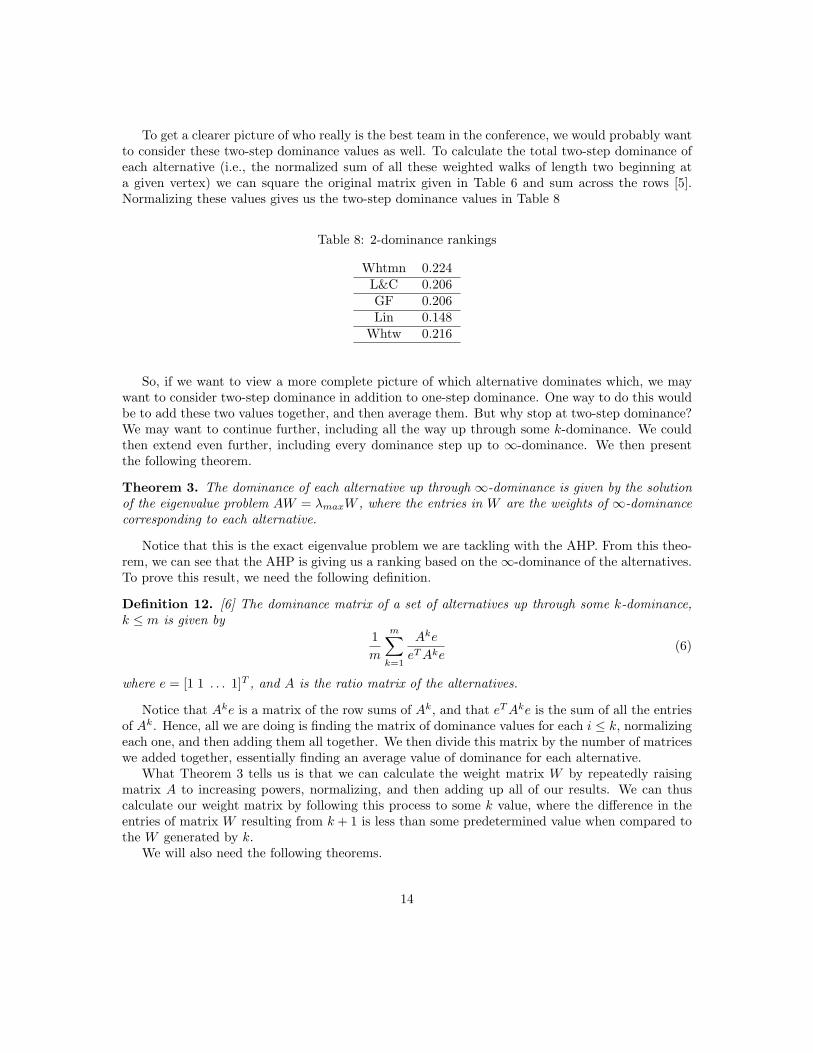
To get a clearer picture of who really is the best team in the conference, we would probably wantto consider these two-step dominance values as well. To calculate the total two-step dominance ofeach alternative (i.e., the normalized sum of all these weighted walks of length two beginning ata given vertex) we can square the original matrix given in Table 6 and sum across the rows [5].Normalizing these values gives us the two-step dominance values in Table 8

Table 8: 2-dominance rankings

Whtmn 0.224L&C 0.206GF 0.206Lin 0.148

Whtw 0.216

So, if we want to view a more complete picture of which alternative dominates which, we maywant to consider two-step dominance in addition to one-step dominance. One way to do this wouldbe to add these two values together, and then average them. But why stop at two-step dominance?We may want to continue further, including all the way up through some k-dominance. We couldthen extend even further, including every dominance step up to ∞-dominance. We then presentthe following theorem.

Theorem 3. The dominance of each alternative up through ∞-dominance is given by the solutionof the eigenvalue problem AW = λmaxW , where the entries in W are the weights of ∞-dominancecorresponding to each alternative.

Notice that this is the exact eigenvalue problem we are tackling with the AHP. From this theo-rem, we can see that the AHP is giving us a ranking based on the ∞-dominance of the alternatives.To prove this result, we need the following definition.

Definition 12. [6] The dominance matrix of a set of alternatives up through some k-dominance,k ≤ m is given by

1

m

m∑k=1

Ake

eTAke(6)

where e = [1 1 . . . 1]T , and A is the ratio matrix of the alternatives.

Notice that Ake is a matrix of the row sums of Ak, and that eTAke is the sum of all the entriesof Ak. Hence, all we are doing is finding the matrix of dominance values for each i ≤ k, normalizingeach one, and then adding them all together. We then divide this matrix by the number of matriceswe added together, essentially finding an average value of dominance for each alternative.

What Theorem 3 tells us is that we can calculate the weight matrix W by repeatedly raisingmatrix A to increasing powers, normalizing, and then adding up all of our results. We can thuscalculate our weight matrix by following this process to some k value, where the difference in theentries of matrix W resulting from k + 1 is less than some predetermined value when compared tothe W generated by k.

We will also need the following theorems.

14

Theorem 4. [4] Let A be a square matrix with all entries aij > 0. Then

limm→∞

(ρ(A)−1A)m = L (7)

where ρ(A) is defined as the maximum of the absolute values of the eigenvalues. Furthermore, wehave the following stipulations: L = xyT , Ax = ρ(A)x, AT y = ρ(A)y, all entries in vectors x andy are greater than 0, and xT y = 1. The vectors x and y are any two vectors that satisfy the givenconditions.

Theorem 5. [3] Let sn be a convergent sequence, that is, let

limn→∞

sn = L

Then

limn→∞

1

n

n∑k=1

sk = L (8)

Thus, we proceed with the proof.

Proof. We can see that the ρ(A) in our case will simply be λmax, and thus the matrix x in Theorem4 must be an eigenvector associated with λmax. Hence, we know that x is some multiple of thenormalized W matrix. With this in mind, let us examine the expression within the summation inequation 6 as m → ∞. We can multiply the limit by one to get the following result:

limm→∞

1λmmax

1λmmax

Ame

eTAme= lim

m→∞

Ak

λmaxe

eT Ak

λmaxe

We know by Theorem 4 that the Ak

λmaxterms are equal to xyT , as defined in that theorem.

Hence, we have:

limm→∞

xyT e

eTxyT e

Note that both x and y are vectors, and so yT e is a scalar, and we can cancel this scalar fromboth numerator and denominator. Hence, we are left with the following result:

x

eTx

Examining the eTx term, we find that this term is simply a scalar equal to the sum of theentries in the x vector. Hence, dividing by this scalar normalizes the vector, giving us W . Then,by Theorem 5, we can see that when we look at the average of the summation of these terms, weget the desired result.

Thus, we now have a theoretical backing to our process. That is, the rankings given by the AHPactually show the ∞-dominance of the alternatives. We can see that the AHP is not just a usefultrick of linear algebra, but that it is actually calculating the ∞-dominance of all of the alternatives.

To give another example of the graphical idea of dominance and how it pertains to decisionproblems, let us again consider the decision problem given in Section 5.2. We can then create a

15

Figure 4: A graphical representation of dominance

corresponding directed graph where each vertex is a criteria, and each edge represents a comparison.Thus, an edge running from CPU to Cost takes on the weight 3, whereas the edge running the otherdirection has weight 1

3 . The graph of this example is shown in Figure 4.We can then think of the weight of the edge as corresponding to dominance. Hence, a one-step

dominance value for Cost is the sum of all the edges emanating from the Cost vertex. This valuewould then be

1

6+

1

3+

1

8=

5

8

To find a two step dominance value, we would start at the Cost vertex and then move to anothervertex. This corresponds to one step. Then, from that vertex, we would follow another edge,multiplying this edge’s value by the previous edge. An example of one of these walks would betaking Cost to Looks, and then Looks to CPU. The value of this two-dominance would then be

1

6× 4 =

2

3

Adding up all such walks through the graph, we find a value for the two-step dominance of Cost.Similarly, we can follow the same procedure for calculating the k-step dominance.

7 Consistency in the AHP

Our whole method for determining the rankings of the alternatives is based on the idea that theyhave some underlying scale. As discussed earlier, this essentially boils down to the idea that when

16

we have calculated our weight matrix, a consistent ratio matrix made using these weights isn’t toofar off of our original ratio matrix. Thus, in order to determine if our results are even valid, wehave to come up with some way of measuring how far off we are. That is, how inconsistent ourratio matrices end up being.

7.1 The CR, CI, and RI

In this section we present the method developed by Saaty [6] for determining inconsistency. Tocreate the tools we need to analyze the inconsistency, we will first need to prove two theorems.

Theorem 6. [6] For a reciprocal n × n matrix with all entries greater than zero, the principaleigenvalue, λmax will be greater than or equal to n. That is, n ≤ λmax.

Proof. Consider some ratio matrix A, and its corresponding consistent ratio matrix A′, which iscreated using the resulting weight eigenvector calculated from A. We know that matrix A hasentries

aij = (1 + δij)(wi/wj)

where 1 + δij is a perturbation from the consistent entry. We know that δij > −1 since none ofour ratio matrices will ever have a negative value or 0 as an entry. (This works out well for theratio matrices we will use, since there is no notion of a “negative preference” in the FundamentalScale–the lowest we can go is 1

9 ). We also know that our matrix A is a reciprocal matrix, and thusfor entry aji, we have:

aji =1

1 + δij(wj/wi)

Thus, setting up our matrix equation AW = λmaxW , we have matrix A as:

A =

1 (1 + δ12)(w1/w2) (1 + δ13)(w1/w3) · · · (1 + δ1n)(w1/wn)

11+δ12

(w2/w1) 1 (1 + δ23)(w2/w3) · · · (1 + δ2n)(w2/wn)1

1+δ13(w3/w1)

11+δ23

(w3/w2) 1 · · · (1 + δ3n)(w3/wn)...

......

. . ....

11+δ1n

(wn/w1)1

1+δ2n(wn/w2)

11+δ3n

(wn/w3) · · · 1(wn/wn)

Since we know matrix A is a reciprocal matrix, we know that the terms in the diagonal must all be1.

We then multiply this matrix by W , which has entries w1, w2, ..., wn, as in the matrix equation.The result is equal to λmaxW . For each element in this matrix, we can look to see that it is equalto the sum of the terms in the corresponding row in matrix A, without the wj in the wi/wj term.Hence, we can divide both sides by wi, and we have an equation giving us λmax for each row.Adding up all of these rows, we have something that is equal to nλmax, where each (1+ δij) occurstwice–once normally, and once as its inverse. Hence, we can find a common denominator and findwhat these terms look like in the sum:

17

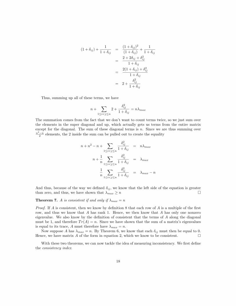
(1 + δij) +1

1 + δij=

(1 + δij)2

(1 + δij)+

1

1 + δij

=2 + 2δij + δ2ij

1 + δij

=2(1 + δij) + δ2ij

1 + δij

= 2 +δ2ij

1 + δij

Thus, summing up all of these terms, we have

n+∑

1≤i<j≤n

2 +δ2ij

1 + δij= nλmax

The summation comes from the fact that we don’t want to count terms twice, so we just sum overthe elements in the super diagonal and up, which actually gets us terms from the entire matrixexcept for the diagonal. The sum of these diagonal terms is n. Since we are thus summing overn2−n

2 elements, the 2 inside the sum can be pulled out to create the equality

n+ n2 − n+∑

1≤i<j≤n

δ2ij1 + δij

= nλmax

n+1

n

∑1≤i<j≤n

δ2ij1 + δij

= λmax

1

n

∑1≤i<j≤n

δ2ij1 + δij

= λmax − n

And thus, because of the way we defined δij , we know that the left side of the equation is greaterthan zero, and thus, we have shown that λmax ≥ n

Theorem 7. A is consistent if and only if λmax = n

Proof. If A is consistent, then we know by definition 8 that each row of A is a multiple of the firstrow, and thus we know that A has rank 1. Hence, we then know that A has only one nonzeroeigenvalue. We also know by the definition of consistent that the terms of A along the diagonalmust be 1, and therefore Tr(A) = n. Since we have shown that the sum of a matrix’s eigenvaluesis equal to its trace, A must therefore have λmax = n.

Now suppose A has λmax = n. By Theorem 6, we know that each δij must then be equal to 0.Hence, we have matrix A of the form in equation 2, which we know to be consistent.

With these two theorems, we can now tackle the idea of measuring inconsistency. We first definethe consistency index.

18

Definition 13. The consistency index (CI) is the value

λmax − n

n− 1(9)

Let us examine what this value actually measures. We know from our theorems that an incon-sistent matrix will have a principal eigenvalue greater than n. Hence, the numerator is essentiallymeasuring how far off the principal eigenvalue is from the consistent case. We then divide this valueby n− 1, which gives us the negative average of the other n− 1 eigenvalues of our matrix [6]. Withthis idea of a consistency index, we can extend further to look at what the CI would be for somecompletely random reciprocal matrix. Moreover, we can find the CI for a large number of thesematrices, and determine an average “random” CI. We then have the following definition.

Definition 14. The random index (RI) of size n is the average CI calculated from a largenumber of randomly generated reciprocal matrices.

In our case, the RI will be determined from 500,000 matrices, randomly generated by computer.For a discussion as to how these matrices were created, see [1]. Given these two definitions, we canmake a third, which will give us a value of the inconsistency.

Definition 15. The consistency ratio (CR) of a reciprocal n × n matrix A is the ratio ofCI(A) : RI(A), where RI(A) is the random index for matrices of size n.

This consistency ratio tells us essentially how inconsistent our matrix is. When running throughthe AHP, if we ever encounter a CR greater than 0.1, we have a ratio matrix that is too inconsistentto give reliable results [6]. In this case, there is not much of an underlying scale present, and theprocess does not work. Thus, if we ever encounter a CR greater than 0.1, we will go back to the ratiomatrix and try to reevaluate our comparisons, until we get a CR that falls within our parameters.For the purposes of this paper, when we encounter a matrix that falls within this tolerance, we willrefer to it as “consistent enough.” Similarly, a matrix that falls outside out tolerances is a matrixwhich is “too inconsistent.”

7.2 Alonso and Lamata’s Approach

We have just seen Saaty’s approach to determining whether a given matrix falls within our tolerancesfor inconsistency. This approach is very involved, and takes several steps after calculating the valueof λmax for the matrix in question. There is an easier way, developed by Alonso and Lamata [1],that allows us to immediately know upon calculation of λmax whether a matrix falls within ourtolerances. This method is presented here, and is the method we will use for the remainder of thepaper when working with examples.

To begin, we first calculate the average value of λmax for a large number of n × n matrices.We will refer to this value as λmax. In Alonso and Lamata’s study, they used 500,000 randomlygenerated matrices for each n, with 3 ≤ n ≤ 13. Note that these are the only values of n we areinterested in for the AHP. For a matrix of size 2, we will always have a consistent matrix, and thusλmax = 2. Furthermore, we split larger matrices into smaller, more manageable sizes (see Section7.3 for a discussion of this process). By finding λmax for the matrices of each size n, Alonso andLamata were able to plot these values against the size of the matrix and find a least-square line tomodel the relationship. The curve that fits the data best is linear, with equation

λmax(n) = 2.7699n− 4.3513 (10)

19

This line fits the data very well, with a correlation coefficient of 0.99 [1].From this data, we can easily calculate the CR for any size of matrix. However, we will argue

that it will be easier to simply use the value of λmax generated by the ratio matrix in question. Thisway, we do not have to do any further calculation after we have found the weight matrix and λmax

in order to determine if the weight matrix is even valid. Hence, we do the following calculations toshow the maximum acceptable value of λmax if we want our CR to be less than 0.1.

First, we know that we can represent the RI for some matrix of size n by

RI =λmax − n

n− 1

Using the definitions of CI and CR (which we want to be less than 0.1), we can then see that

CR =λmax − n

λmax − n< 0.1

Solving for λmax, we haveλmax < n+ 0.1(λmax − n)

Thus, combining this result with our equation 10, we see that

λmax < 1.17699n− 0.43513 (11)

Using this equation, we can determine the maximum allowable λmax for an n×n matrix by simplycalculating 1.17699n−0.43513. If our λmax is less than this value, then our matrix will still be withinthe allowable inconsistency, and we don’t have to mess with the CI, CR, or RI at all. Furthermore,we can follow these same calculations to determine the allowable λmax for other tolerances. If weare less concerned with the consistency of our data, and would rather not have to go back andreevaluate ratio matrices, we might pick a value larger than 0.1. For instance, if we were to allowa more inconsistent matrix, we could go up to a tolerance of 20%, which would correspond to aCR less than 0.2. Then, following through the same calculations here, we would come up with theequation

1.55398n− 0.87026

Given equation 11 we can create a table of the maximum allowable λmax for a matrix of size n.From this table, we can easily determine if a given ratio matrix falls within our tolerances, or if wehave to go back and try again. This table will be very useful as we go further in this paper. It ispresented as Table 9.

Table 9: The maximum accepted λmax for an n× n matrix [1]

n λmax n λmax

3 3.0957 8 8.98064 4.2727 9 10.15765 5.4497 10 11.33466 6.6266 11 12.51667 7.8036 12 13.6886

20

Note that as we create larger and larger matrices, the largest allowable λmax gets further andfurther from the n in question. This alludes to the idea that as we compare more and morealternatives, our results from the AHP are “less accurate.” Methods for dealing with this problemare dealt with in the following section.

7.3 Clustering

(note: While working through this section, readers may find it helpful to refer to the worked ex-ample of clustering given in Section 7.3.1).

So far we have discussed AHP problems and examples with relatively few criteria and alterna-tives. In these cases, we can proceed just as we have been without getting too worried that thenumber of elements we are comparing could be contributing to error. As we look at more and morealternatives however, there certainly is more and more room for judgment error, leading to a lessconsistent result. Clustering allows us to look at the problem on a smaller scale which we are moreused to, and then expand to the rest of the elements. Because we want to minimize inconsistency,whenever we are looking at more than 9 elements, be they alternatives or criteria, we will proceedby clustering our elements.

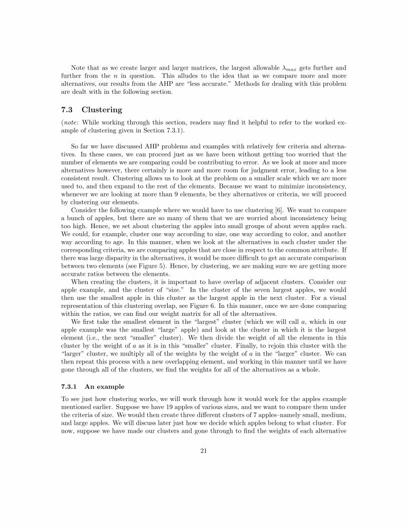
Consider the following example where we would have to use clustering [6]. We want to comparea bunch of apples, but there are so many of them that we are worried about inconsistency beingtoo high. Hence, we set about clustering the apples into small groups of about seven apples each.We could, for example, cluster one way according to size, one way according to color, and anotherway according to age. In this manner, when we look at the alternatives in each cluster under thecorresponding criteria, we are comparing apples that are close in respect to the common attribute. Ifthere was large disparity in the alternatives, it would be more difficult to get an accurate comparisonbetween two elements (see Figure 5). Hence, by clustering, we are making sure we are getting moreaccurate ratios between the elements.

When creating the clusters, it is important to have overlap of adjacent clusters. Consider ourapple example, and the cluster of “size.” In the cluster of the seven largest apples, we wouldthen use the smallest apple in this cluster as the largest apple in the next cluster. For a visualrepresentation of this clustering overlap, see Figure 6. In this manner, once we are done comparingwithin the ratios, we can find our weight matrix for all of the alternatives.

We first take the smallest element in the “largest” cluster (which we will call a, which in ourapple example was the smallest “large” apple) and look at the cluster in which it is the largestelement (i.e., the next “smaller” cluster). We then divide the weight of all the elements in thiscluster by the weight of a as it is in this “smaller” cluster. Finally, to rejoin this cluster with the“larger” cluster, we multiply all of the weights by the weight of a in the “larger” cluster. We canthen repeat this process with a new overlapping element, and working in this manner until we havegone through all of the clusters, we find the weights for all of the alternatives as a whole.

7.3.1 An example

To see just how clustering works, we will work through how it would work for the apples examplementioned earlier. Suppose we have 19 apples of various sizes, and we want to compare them underthe criteria of size. We would then create three different clusters of 7 apples–namely small, medium,and large apples. We will discuss later just how we decide which apples belong to what cluster. Fornow, suppose we have made our clusters and gone through to find the weights of each alternative

21

Figure 5: Circles A and B are the same size in each comparison, but when they are put with acircle closer to their size, it is easier to estimate just how much larger one is than the other [7]

just as we always have, but only focusing on one cluster at a time. Suppose we found the weightsfor the size of the apples as given in Table 10.

Note that the columns of this table are simply the normalized weight matrices that we arefamiliar with. The only difference is that they aren’t the overall weights, but instead the weightsfor a small sample given by each cluster. We will eventually refine the weights in this table to get thefinal overall weights. Note also that the largest apple in the small cluster is also the smallest applein the medium cluster, even though they have different weights. This is because when comparedwithin either cluster, they will certainly have different weights because of the apples they are beingcompared to. Similarly, the largest medium apple is the same as the smallest large apple. We canthen create a weight matrix for all of our alternatives by the following process. First, bring themedium cluster into conjunction with the large cluster by dividing by the largest medium apple’sweight and then multiplying by the smallest large apple’s weight (really, these two weights are thesame since they come from the same apple). We then get a weight matrix for all of the apples inthe medium cluster (given in 12) which now is a part of the large cluster, and so all the weightsmake sense within that cluster.

22

Figure 6: The structure of the “medium” and “large” clusters.

Table 10: The relative weights of apples under the criterion “size” by clustering

Small Medium Large

0.045 0.088 0.086

0.103 0.118 0.094

0.121 0.132 0.120

0.134 0.145 0.142

0.179 0.162 0.167

0.205 0.171 0.176

0.214 0.184 0.215

23

1

0.184

0.0880.1180.1320.1450.1620.1710.184

0.086 =

0.0410.0550.0620.0680.0760.0800.086

(12)

We then do the same thing for the small cluster, using our new value for the smallest “large”apple, 0.041.

1

0.214

0.0450.1030.1210.1340.1790.2050.214

0.041 =

0.0090.0200.0230.0260.0340.0390.041

Hence, combining our new found weight matrices with the matrix for the large cluster, we find thatthe weight matrix for size out of these 19 apples:

0.0090.0200.0230.0260.0340.0390.0410.0550.0620.0680.0760.0800.0860.0940.1200.1420.1670.1760.215

which we would then normalize. Note that the entries in red are the “overlapping” alternatives.

We must now figure out just how we are going to create these clusters. In the example of applesof various sizes, it is easy to see how we could decide which apples belonged to which cluster, andcould easily place them. However, with more abstract criteria and alternatives, the decision is notalways as easy.

24

Saaty gives three possible approaches to determining clusters, ranked by least to most efficient[6]. The first of these is called the elementary approach. It is very simple and intuitive, but notvery effective. It works by simple comparison. Given n alternatives, we can pick one out from thebunch. Then, working our way through the rest of the other alternatives, we compare pairwisewith our selected alternative. If a compared alternative beats out the one we selected (if we findan apple bigger that the one in our hand, for example), we have a new “largest” alternative, andwe continue comparing. Once we have found the largest, we would repeat the process with thisalternative removed, trying to find the second largest. As can be seen, we would have to go through(n− 1)! comparisons just to figure out our clustering [6].

The second proposed method is called trial and error clustering. In this process, we try to getan idea of what the clusters would reasonably look like. We make three general groups, “large,”“medium,” and “small.” We could look through the alternatives, see which looked to fit where(“that apple looks pretty small, we should probably put it in the small category”), and place themtemporarily. We then place the alternatives in each group into several clusters, and make a passthrough, making comparisons. Any misfits are moved to one of the other two groups. We thenre-cluster, and make another comparison pass, again moving the misfits. After these two passes,the clusters should be reasonable enough that we can carry out our process as in the example.

The most efficient method is clustering by absolute measurement. In absolute measurement, thegroup looks at each alternative and tries to assign a weight without going through the whole AHP.This way, general clusters can be formed and then put through the AHP. The clusters are alreadycomprised of elements that the group thinks go together, and the AHP simply refines the weightthat they have assigned by using pairwise comparisons between the alternatives, rather than tryingto assign some arbitrary number to each alternative.

8 Paradox in the AHP

We have now seen that there are matrices that are so inconsistent that they are weeded out beforethey even make it into our calculations to determine rankings. In this way, we discard matrices thatcould potentially give us rankings that aren’t consistent with the ideas behind the AHP. However,what if we could create matrices that are within our tolerances for inconsistency, but, by their verystructure, give paradoxical results? This section will examine some examples of these paradoxes,and will discuss the implications they have on the AHP.

8.1 Perturbing a Consistent Matrix

The first method we will examine for creating a paradox is that of simply making small alterationsto a consistent matrix. In this example we will examine 5 alternatives, with weight matrix given inTable 11.

This weight matrix was created by assigning each alternative a weight from 2 to 6, and thennormalizing the weight matrix. From this matrix, we could then create the consistent ratio matrix.However, in order to create a paradox, we change the preference ratio of A : B in the ratio matrix.Hence, instead of a12 = 0.4 (which is simply 0.105/0.263, which we got from the weights of eachalternative), we have a12 = 5, which we assign. We do the same swap with a21, changing it to 0.2,or the inverse of 5. By doing this, we want to see if making one small change will go “unnoticed”when we calculate the new weight matrix. We then have the result shown in equation 13. Notethat the changed entries are shown in red.

25

1 5 0.5 1 0.3330.2 1 1.25 2.5 0.8332 0.8 1 2 0.6661 0.4 0.5 1 0.3333 1.2 1.5 3 1

0.2290.1640.2030.1010.304

= 5.909

0.2290.1640.2030.1010.304

(13)

As we can see, our new weight matrix recognized the change we made, and adjusted accordingly.Now, since we decided we preferred A to B, even though the rest of the matrix is consistent withthe case where we preferred B to A, the weight matrix tells us that A is a better choice than B.So, we can see that the process picked up on the change we made to just one entry. This onechange does give us an eigenvalue that is outside of our acceptable range of inconsistency however,indicating how much changing just one entry from the consistent matrix can result in relativelylarge inconsistency (note also that since the original ratio matrix was consistent, it would have hada λmax of 5 by Theorem 7).

We have now seen just how little it takes to upset a consistent matrix. Thus, we now try tocreate a matrix that falls within our tolerances for inconsistency. Let us try by changing the alteredentry to 2 rather than 5, which indicates a less drastic reversal of preference. Hence, we have thenew weight matrix for our alternatives given in Table 12.

Note that this weight matrix still retains the original preference of B over A as given in Table11, and that the matrix falls within our tolerances for inconsistency.

Let us take a moment to consider what this situation tells us. When going through pairwisecomparisons, we decided that alternative A was preferable to B. However, once we ran throughthe AHP, we are told that in actuality alternative B is preferable to alternative A. On one hand,we could argue that although alternative A is preferable to alternative B when we only considerthose two alternatives, we are comparing A to B only. We are not taking into account any of theother alternatives, even though we are trying to decide which alternative is best out of a group of5, not just a group consisting of A and B. While A may be preferable to B pairwise, the weightmatrix tells us that alternative B is preferable to A in the larger scheme of things. This argumentmay be acceptable given certain situations. Consider the example of basketball teams playing oneanother given in Section 6. Although George Fox beat Whitworth, when we take into account allof the other teams, Whitworth actually did better in the conference.

This argument certainly makes sense for the given problem, but consider an entirely differentsituation. Now suppose we are back choosing a computer for the math lab given in Section 5.2, andwe are choosing between 5 computers. Suppose we are evaluating based on the “looks” criterion,and so are trying to determine the prettiest computer. When comparing pairwise, we note thatcomputer A looks better than computer B, but when we calculate the weight matrix, we find Table

Table 11: The weight matrix for our 5 alternatives

A 0.105B 0.263C 0.210D 0.105E 0.316

26

Table 12: The new weight matrix: λmax = 5.336

A 0.166B 0.201C 0.211D 0.105E 0.316

12. Supposedly, given our pairwise rankings, B actually looks better than A. However, what if westart removing alternatives? If we take away all of the computers other than A and B, we see thatthe weight matrix tells us B is a more attractive option than A, which we know to be false. In thiscase, the paradox found does not makes sense given the problem.

This example illustrates several aspects of a paradox of this nature. First, we see that we canonly perturb the matrix by a small amount. With a completely consistent matrix, we were onlyable to change one entry by a small amount before we were suddenly outside our tolerances forinconsistency. Moreover, we noticed that the paradoxical nature of the matrix is dependent on theactual problem we are looking at. This idea that the results must be interpret based on the originalproblem is crucial to the AHP. We cannot blindly follow our calculations without first consideringwhat they are telling us.

8.2 Preference Cycles

The second paradox we will look at arises from the idea of preference cycles, which we define here.

Definition 16. A preference cycle is a set of n elements with weights w1, w2, . . . , wn such that

w1 > w2 > · · · > wi > wi+1 > · · · > wn > w1

A real world example of a preference cycle is the game of rock, paper, scissors, where eachelement beats exactly one other element, and loses to exactly one other element.

With this definition in mind, we will look to create a consistent weight matrix that arises from asituation where there is a preference cycle. Note that in the previous paradox example, a preferencecycle arose when we changed the preferences of A and B. In this example, we will look what happenswith a ratio matrix created solely from preference cycles. Hence, consider the ratio matrix for sixalternatives given in Table 13.

Note that we have the preference cycle A > B > C > D > E > F > A, and that the matrix iswithin our inconsistency tolerances.

The case that we have presented here is interesting because of what the AHP tells us about ouralternatives. When the weight matrix is calculated, we find that every alternative has the sameweight. That is, we see that no one alternative is any better than another, which makes sense giventhe problem. Moreover, we can have alternatives that make no sense within a standard scale, butstill pass our tolerances for inconsistency and give us some kind of result that is (by way of theAHP), in a standard scale. If we think back to our rock-paper-scissors example, the results shownabove make sense. Given two pairings, we can obviously choose one alternative over the other, orelse the two alternatives are equal (that is, neither player wins). However, before the game starts,

27

Table 13: The ratio matrix for a preference cycle of six elements- λmax = 6.5

A B C D E FA 1 2 1 1 1 1

2

B 12 1 2 1 1 1

C 1 12 1 2 1 1

D 1 1 12 1 2 1

E 1 1 1 12 1 2

F 2 1 1 1 12 1

we have no idea what the other player will show, and so every alternative is just as good as any.This is represented in the weight matrix by equivalent weights for each alternative, and in the ratiomatrix by the parities entries. For the given example in Table 13, the 6 × 6 matrix is the firstinstance when we are within our inconsistency tolerances.

8.3 Further Paradoxes

These two examples are interesting in their own right, but there are many more possibilities forparadox within the AHP. Since it was not the goal of this paper to investigate paradoxes specifically,and since there is not a lot of available research on the types of problems illustrated here, we willstop our investigation of paradox here. We will however present some interesting extensions on thetopic, which can be explored further.

First, much of the background and ideas for creating paradoxes in this paper arose from researchinto voting theory [2]. Thus, the idea of “strategic voting” (wherein an individual or small groupcan exploit the voting system to a desired end) is a natural extension of the idea of paradox withinthe AHP. Moreover, since the AHP is used often in business when meaningful, costly decisions arebeing made, it would be important to know whether the system can be subversively exploited by anindividual or small group. As was illustrated in Section 8.1, it is possible to prefer one alternativeover another, only to have the AHP tell you that actually, the preference should be the other wayaround.

Furthermore, it would be interesting to see which kinds of matrices are more susceptible toparadox. We have seen that larger matrices allow for more inconsistency (as indicated by Table9), so we would think that these larger matrices would have more room for giving strange results.Another question to address would be to see if we could “spread out” the inconsistency morethroughout the matrix, or if it is solely matrices that are almost perfectly consistent that allow forparadox.

One area of research that has been looked into, but which was not really discussed in this paper,is that of adding and subtracting alternatives and criteria. In an ideal process, simply adding orremoving alternatives should do nothing to change the rank order of the alternatives, but this isnot always the case. We alluded to this idea with the computer’s “looks” in Section 8.1, but didnot discuss at length.

28

9 An Applied AHP Problem

Now that we have a thorough understanding of the AHP, we will see just how it works in a realworld decision problem. In this section, we look at the difficult decision of deciding where to attendgraduate school given several choices. For this problem, we surveyed a senior at Whitman Collegewho had been accepted to five schools for graduate chemistry programs. Thus, we define the prob-lem as follows.

The goal: to choose the best graduate school for a particular individual (Tyler, our dauntlessscholar).

9.1 The Criteria

These criteria were determined by speaking with Tyler, and figuring out what was important tohim for choosing a grad school. Within each criterion, any sub-criteria are given in italics.

Location: Simply, where the school is located. This criteria has three sub-criteria makingup what the “location” really entails. Weather is certainly an important factor to consider whenpicking a school. Just look at the difference between winters in the midwest and winters in southernCalifornia. The type of municipality the school is in also comes into play. Rural and urban schoolsoffer different things when it comes to life outside of campus, and it is important to consider whatkind of city or town you will be living in. Location can also mean how far away you are from thethings you care about. Distance from your family and friends can be a good thing or a bad thingdepending on how you look at it.

Financial Incentive: This criterion reflects the amount of money the school is willing to give,as well as the cost of living in the city where the school is located.

Ranking: Certainly ranking is important when choosing a school. The name Harvard carriesmuch more weight than a local community college. This ranking can be looked at from two angles.First, the prestige associated with the name and school can be considered. Second, the numericalrankings published by various sources such as US News and World Report. Both of these factorscarry some weight when trying to evaluate a school’s rank.

Degree Program: It is important to consider what the degree program at each universityactually entails. Some may have more limiting requirements, while others may require excitinghands-on research. Either way, it is an important factor to consider when making a decision aboutwhat school to go to.

Campus: The school’s campus can be large or small, beautiful or ugly, and either way, itfactors into the decision of what school to go to. The grounds of the school may be beautiful, withplenty of open fields, or they may be small and largely concrete. The buildings on campus are alsoimportant to consider. Is there a good library? Are the classrooms nice? Is there an on campuscoffee shop where I can study? Finally, since we are dealing with a chemistry student, it is alsoimportant to factor in the labs when making a decision.

Faculty: The school itself may be great, but without excellent faculty, it isn’t really worthchoosing. Here we look at two factors, the student’s potential advisor, and the rest of the department.

Vibe: This is a very important factor when choosing a school, but it is hard to quantify. Theintangible feeling you get when walking around campus, and how you feel when you picture yourselfgoing to a certain school are certainly very important in the final decision.

29

9.2 The Alternatives

For this decision problem, we considered the following five schools:

• The University of California, Berkeley. We will denote this alternative as simply “Berkeley.”

• The University of Wisconsin, Madison, which we will denote “Madison.”

• The University of Chicago, which we will denote “Chicago.”

• The University of California, San Diego, which we will denote “UCSD.”

• The University of Washington, Seattle, which we will denote “UW.”

These schools comprise our alternatives. Hence, given the decision problem, we can lay out ahierarchy as illustrated in Figure 7.

Figure 7: The hierarchy for our grad school problem

30

9.3 Gathering Data

After clearly defining the decision problem, the next step is to determine the ratio matrices foreach criterion and alternative. We determined that the easiest way to do this would be through aworksheet of sorts, where Tyler could give scores for each comparison based on Saaty’s fundamentalscale (see Table 15). An example of one of these sheets is given in Table 16. Once all of this datawas collected, we were able to create corresponding ratio and weight matrices for each criterion andalternative. These results are presented in Tables 17 through 52. Recall that when looking at thesematrices, the preferences are read as row over column. That is, the number in entry aij representshow much alternative i is preferred over alternative j, according to the standard scale.

9.4 Determining the Final Weight Matrix

Just as we did in the computer example in Section 5.2, we simply multiply our way back up thehierarchy. For instance, tracing up “Madison” from its weight in the “Buildings” matrix, we firstmultiply the weight of “Madison” in this matrix by the weight of “Buildings” in its sub-criteriaweight matrix. Then, this result is multiplied by the weight of “Campus” in its criteria matrix. Wedo this for every school, and for every path up the hierarchy. When we have all of these results, weadd them up for each school. That is, all the weights for each school are summed separately, andthese values become the final weight of the schools, giving us our result. The final weights fromthese calculations can be found in Table 14.

Table 14: Alternative Weight Matrix–“Overall”

School WeightBerkeley 0.4350Madison 0.2172Chicago 0.1743UCSD 0.0706UW 0.1060

As can be seen, Berkeley is the school that best satisfies our original goal of choosing the bestgrad school for Tyler, and by a generous margin. Before going through the process, Tyler statedthat he was not sure where he was going to go. He knew that Berkeley and Madison were the twotop contenders, and was interested to see if the process could set them apart from each other. Withthe results in Table 14, it is plain to see that the AHP is a powerful tool in making tough decisions.

Note that we can look at the “intermediate hierarchies” as well. If we were interested in whatschool best fulfilled the “campus resources” criterion, we could follow the same process as we didto calculate the values given in Table 14, but taking “campus” as the goal of our problem. Hence,the “campus resources” sub-criteria become the criteria in this problem. In this case, it turns outthat Chicago best satisfies the goal. If Tyler was making his choice exclusively on how good thecampus was, then Chicago would be the best bet. From this, we can see that Berkeley did not winout every criterion, and yet still won overall. This goes further to show how powerful a tool theAHP is. Even though an alternative does not win outright in every category, when everything istaken into account, we can find that the alternative is best given the entire problem.

31

9.5 Thoughts on the Applied Problem

By working through this problem, we have discovered just how straightforward and useful a toolthe AHP is. A decision that was originally locked in stalemate was handily resolved by simplepairwise comparisons and some linear algebra. Moreover, we have seen just how easy it is to gatherthe data necessary to run through the process given just one person making the decision. If wewere instead working through a problem that dealt input from multiple people, we would have todevise some way of fairly aggregating the responses of each individual. This aspect of the AHPwas not investigated in this paper, nor was it discussed in Saaty’s article [6]. It is certainly a veryimportant aspect to decision problems, and should be considered when using the AHP to resolvegroup choices.

We have also shown (in our particular scenario) that it is not terribly difficult to arrive at weightmatrices that are within our tolerances for inconsistency. Working through this problem, we hadonly one weight matrix out of 11 that was outside of our tolerance (the “urban/rural” alternativematrix). For this matrix, we went back and reevaluated the corresponding ratio matrix by runningthrough the pairwise comparisons again, and quickly reached a weight matrix that fell within ourtolerance.

10 Conclusions and Ideas for Further Research

As we have seen, the AHP is a useful, applicable tool to many situations in life. We are faced withdecision problems every day, and often these are difficult to solve. With the AHP, we now have anexcellent method for turning these difficult, incorporeal questions into reliable mathematics, fromwhich we can easily determine a solution.

Furthermore, we have seen that this process is relatively easy. Solely through pairwise compar-ison and simple linear algebra, we can arrive at some powerful results. Moreover, these results ac-tually mean something. That is, by running through the AHP we are calculating the ∞-dominanceof the alternatives in question. Rather than a fancy trick of linear algebra, we actually have sometheoretical backing to our results.

We have also seen that the process is resistant to strange results. By creating inconsistencytolerances, we get rid of many matrices that disagree with the principles at work in the AHP.However, this does not mean that the process is perfect, and completely foolproof. There are stillpossibilities for paradox and illogical results even with the inconsistency tolerances in place.

This is one very intriguing area of further research. While we have only presented two para-doxes in this paper, there are certainly countless more examples that can be dreamt up. A closerexamination of some of these could prove to be very interesting indeed, as well as shedding lighton just what can go wrong in the AHP. The specific idea of “strategic voting,” a term borrowedfrom voting theory, would be very interesting. Since the AHP is used often in the business worldto make important decisions, it would be worthwhile to investigate just how much one individualor a small group could strategically affect the overall rankings of the alternatives.

Additionally, further research into the kinds of problems the AHP is used to look at could bevery interesting. Specifically, the area of sports problems (such as the basketball example givenin Section 6) would be an attractive application. As far as I know, there has not been a lot ofinvestigation as to using the AHP to look at these kinds of problems, but it seems like they are aprime situation for analysis by the process.

As I only conducted an applied problem for one person, gathering the data for the comparisons

32

was relatively easy. It would be interesting to research different methods of gathering this data froma group of people, rather than an individual. This would certainly be a worthwhile investigation,since decisions are often made by groups rather than individuals, and we need an effective wayof gathering and consolidating the opinions from everyone in the group. Moreover, it would beinteresting to look at the differences between one of these group AHP problems compared to anindividual AHP problem.

33

11 Appendix

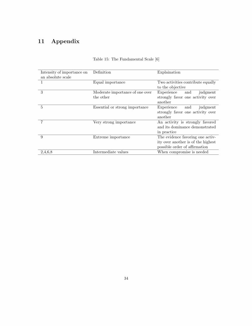
Table 15: The Fundamental Scale [6]

Intensity of importance onan absolute scale

Definition Explaination

1 Equal importance Two activities contribute equallyto the objective

3 Moderate importance of one overthe other

Experience and judgmentstrongly favor one activity overanother

5 Essential or strong importance Experience and judgmentstrongly favor one activity overanother

7 Very strong importance An activity is strongly favoredand its dominance demonstratedin practice

9 Extreme importance The evidence favoring one activ-ity over another is of the highestpossible order of affirmation

2,4,6,8 Intermediate values When compromise is needed

34

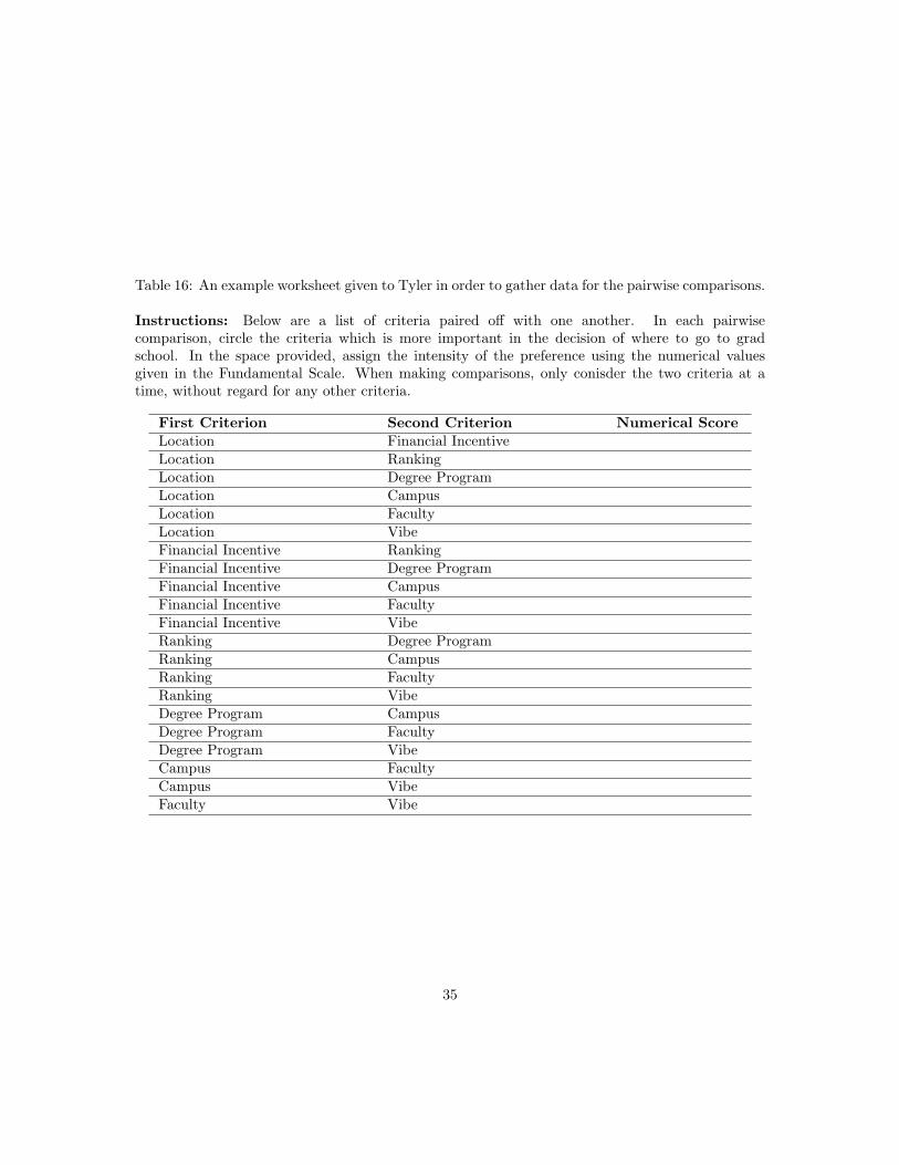
Table 16: An example worksheet given to Tyler in order to gather data for the pairwise comparisons.

Instructions: Below are a list of criteria paired off with one another. In each pairwisecomparison, circle the criteria which is more important in the decision of where to go to gradschool. In the space provided, assign the intensity of the preference using the numerical valuesgiven in the Fundamental Scale. When making comparisons, only conisder the two criteria at atime, without regard for any other criteria.

First Criterion Second Criterion Numerical ScoreLocation Financial IncentiveLocation RankingLocation Degree ProgramLocation CampusLocation FacultyLocation VibeFinancial Incentive RankingFinancial Incentive Degree ProgramFinancial Incentive CampusFinancial Incentive FacultyFinancial Incentive VibeRanking Degree ProgramRanking CampusRanking FacultyRanking VibeDegree Program CampusDegree Program FacultyDegree Program VibeCampus FacultyCampus VibeFaculty Vibe

35

Table 17: Criteria Ratio Matrix

Loc. Fin. Rank Degree Camp. Fac. VibeLoc. 1 5 6 6 4 1

314

Fin. 15 1 1

2 2 13

14

17

Rank 16 2 1 3 1

315

16

Degree 16

12

13 1 1

315

17

Camp. 14 3 3 3 1 1

314

Fac. 3 4 5 5 3 1 15

Vibe 4 7 6 7 4 5 1

Table 18: Criteria Weight Matrix (Eigenvalue = 7.736)

Criterion WeightLoc. 0.1731Fin. 0.0383Rank 0.0490Degree 0.0286Camp. 0.0838Fac. 0.2074Vibe 0.4198

Table 19: Location Sub-Criteria Ratio Matrix

Weather Rural/Urban DistanceWeather 1 4 1

3

Rural/Urban 14 1 1

6

Distance 3 6 1

Table 20: Location Sub-Criteria Weight Matrix (Eigenvalue = 3.054)

Sub-Criterion WeightWeather 0.2704

Rural/Urban 0.0852Distance 0.6444

36

Table 21: Rankings Sub-Criteria Ratio Matrix

Prestige RankingsPrestige 1 3Rankings 1

3 1

Table 22: Rankings Sub-Criteria Weight Matrix (Eigenvalue = 2)

Sub-Criterion WeightPrestige 0.75Rankings 0.25

Table 23: Campus Sub-Criteria Ratio Matrix

Grounds Buildings LabsGrounds 1 1

316

Buildings 3 1 15

Labs 6 5 1

Table 24: Campus Sub-Criteria Weight Matrix (Eigenvalue = 3.094)

Sub-Criterion WeightGrounds 0.0883Buildings 0.1946

Labs 0.7171

37

Table 25: Faculty Sub-Criteria Ratio Matrix

Potential Advisor Rest of DepartmentPotential Advisor 1 1

4

Rest of Department 4 1

Table 26: Faculty Sub-Criteria Weight Matrix (Eigenvalue = 2)

Sub-Criterion WeightPotential Advisor 0.2Rest of Department 0.8

Table 27: Alternative Ratio Matrix–“Weather”

Berkeley Madison Chicago UCSD UWBerkeley 1 6 7 1

3 4Madison 1

7 1 2 17 2

Chicago 17

12 1 1

7 2UCSD 3 7 7 1 8UW 1

412

12

18 1

Table 28: Alternative Weight Matrix–“Weather” (Eigenvalue = 5.283)

School WeightBerkeley 0.2928Madison 0.0790Chicago 0.0589UCSD 0.5207UW 0.0486

38

Table 29: Alternative Ratio Matrix–“Urban/Rural”

Berkeley Madison Chicago UCSD UWBerkeley 1 4 6 3 1

3

Madison 14 1 4 4 1

5

Chicago 16

14 1 1

416

UCSD 13

14 4 1 1

5

UW 3 5 6 5 1

Table 30: Alternative Weight Matrix–“Urban/Rural” (Eigenvalue = 5.436)

School WeightBerkeley 0.2725Madison 0.1371Chicago 0.0404UCSD 0.0882UW 0.4618

Table 31: Alternative Ratio Matrix–“Distance”

Berkeley Madison Chicago UCSD UWBerkeley 1 5 4 7 2Madison 1

5 1 13 5 1

4

Chicago 14 3 1 5 1

4

UCSD 17

15

15 1 1

7

UW 12 4 4 7 1

Table 32: Alternative Weight Matrix–“Distance” (Eigenvalue = 5.384)

School WeightBerkeley 0.4255Madison 0.0870Chicago 0.1413UCSD 0.0343UW 0.3119

39

Table 33: Alternative Ratio Matrix–“Prestige”

Berkeley Madison Chicago UCSD UWBerkeley 1 4 6 8 8Madison 1

4 1 3 5 5Chicago 1

613 1 3 3

UCSD 18

15

13 1 1

2

UW 18

15

13 2 1

Table 34: Alternative Weight Matrix–“Prestige” (Eigenvalue = 5.228)

School WeightBerkeley 0.5614Madison 0.2289Chicago 0.1104UCSD 0.0428UW 0.0565

Table 35: Alternative Ratio Matrix–“Ranking”

Berkeley Madison Chicago UCSD UWBerkeley 1 4 5 6 8Madison 1

4 1 3 4 6Chicago 1

513 1 3 5

UCSD 16

14

13 1 3

UW 18

16

15

13 1

Table 36: Alternative Weight Matrix–“Ranking” (Eigenvalue = 5.330)

School WeightBerkeley 0.5293Madison 0.2347Chicago 0.1311UCSD 0.0689UW 0.0360

40

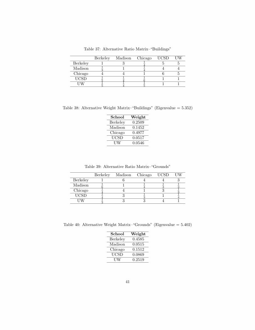
Table 37: Alternative Ratio Matrix–“Buildings”

Berkeley Madison Chicago UCSD UWBerkeley 1 3 1

4 5 5Madison 1

3 1 14 4 4

Chicago 4 4 1 6 5UCSD 1

514

16 1 1

UW 15

14

15 1 1

Table 38: Alternative Weight Matrix–“Buildings” (Eigenvalue = 5.352)

School WeightBerkeley 0.2509Madison 0.1452Chicago 0.4977UCSD 0.0517UW 0.0546

Table 39: Alternative Ratio Matrix–“Grounds”

Berkeley Madison Chicago UCSD UWBerkeley 1 6 4 4 3Madison 1

6 1 14

13

13

Chicago 14 4 1 3 1

3

UCSD 14 3 1

3 1 14

UW 13 3 3 4 1

Table 40: Alternative Weight Matrix–“Grounds” (Eigenvalue = 5.402)

School WeightBerkeley 0.4585Madison 0.0515Chicago 0.1512UCSD 0.0869UW 0.2519

41

Table 41: Alternative Ratio Matrix–“Labs”

Berkeley Madison Chicago UCSD UWBerkeley 1 4 1

2 6 5Madison 1

4 1 15 4 3

Chicago 2 5 1 6 5UCSD 1

614

16 1 1

3

UW 15

13

15 3 1

Table 42: Alternative Weight Matrix–“Labs” (Eigenvalue = 5.324)

School WeightBerkeley 0.3113Madison 0.1278Chicago 0.4347UCSD 0.0417UW 0.0733

Table 43: Alternative Ratio Matrix–“Potential Advisor”

Berkeley Madison Chicago UCSD UWBerkeley 1 1 2 6 5Madison 1 1 2 6 5Chicago 1

212 1 5 4

UCSD 16

16

15 1 1

2

UW 15

15

14 2 1

Table 44: Alternative Weight Matrix–“Potential Advisor” (Eigenvalue = 5.070)

School WeightBerkeley 0.3384Madison 0.3384Chicago 0.2078UCSD 0.0465UW 0.0687

42

Table 45: Alternative Ratio Matrix–“Rest of Department”

Berkeley Madison Chicago UCSD UWBerkeley 1 4 5 6 8Madison 1

4 1 3 5 6Chicago 1

513 1 3 5

UCSD 16

15

13 1 3

UW 18

16

15

13 1

Table 46: Alternative Weight Matrix–“Rest of Department” (Eigenvalue = 5.353)

School WeightBerkeley 0.5269Madison 0.2431Chicago 0.1287UCSD 0.0659UW 0.0353

Table 47: Alternative Ratio Matrix–“Financial Incentive”

Berkeley Madison Chicago UCSD UWBerkeley 1 1

316 3 1

4

Madison 3 1 13 4 1

3

Chicago 6 3 1 7 5UCSD 1

314

17 1 1

6

UW 4 3 15 6 1

Table 48: Alternative Weight Matrix–“Financial Incentive” (Eigenvalue = 5.410)

School WeightBerkeley 0.0697Madison 0.1394Chicago 0.5174UCSD 0.0390UW 0.2345

43

Table 49: Alternative Ratio Matrix–“Degree Program”

Berkeley Madison Chicago UCSD UWBerkeley 1 4 5 6 6Madison 1

4 1 3 4 5Chicago 1

513 1 3 4

UCSD 16

14

13 1 2

UW 16

15

14

12 1

Table 50: Alternative Weight Matrix–“Degree Program” (Eigenvalue = 5.320)

School WeightBerkeley 0.5231Madison 0.2349Chicago 0.1305UCSD 0.0652UW 0.0463

Table 51: Alternative Ratio Matrix–“Vibe”

Berkeley Madison Chicago UCSD UWBerkeley 1 3 4 6 5Madison 1

3 1 3 5 4Chicago 1

413 1 4 3

UCSD 16

15

14 1 1

3

UW 15

14

13 3 1

Table 52: Alternative Weight Matrix–“Vibe” (Eigenvalue = 5.314)

School WeightBerkeley 0.4704Madison 0.2620Chicago 0.1440UCSD 0.0446UW 0.0791

44

References

[1] Jose Alonso and Teresa Lamata, Consistency in the Analytic Hierarchy Process: A New Ap-proach. International Journal of Uncertainty, Fuzziness and Knowledge-Based Systems. Vol. 14,No. 4 (2006) 445-459.

[2] Steven J. Brams, Mathematics and Democracy: Designing better voting and fair-division proce-dures. Princeton University Press. (2008).

[3] Godfrey Harold Hardy, Divergent Series. Clarendon Press, Oxford. (1956).

[4] Roger A. Horn, Charles R. Johnson, Matrix Analysis. Cambridge University Press, Cambridge.(1985).

[5] David C. Lay, Linear Algebra and its Applications, Third Edition Addison Wesley, 2006. Page114.

[6] Thomas Saaty, How to make a decision: The Analytic Hierarchy Process. European Journal ofOperational Research 48 (1990) 9-26. North Holland

[7] Xiaojun Yang, Liaoliao Yan, and Luan Zeng How to handle uncertainties in AHP: The CloudDelphi hierarchical analysis. Journal of Information Sciences 222 (2013) 384-404.

45