mathematical methods in quantum...
TRANSCRIPT
Mathematical Methodsin Quantum Mechanics
With Applications to Schrodinger Operators
Gerald Teschl
Gerald TeschlFakultat fur MathematikNordbergstraße 15Universitat Wien1090 Wien, Austria
E-mail: [email protected]: http://www.mat.univie.ac.at/˜gerald/
2000 Mathematics subject classification. 81-01, 81Qxx, 46-01
Abstract. This manuscript provides a self-contained introduction to math-ematical methods in quantum mechanics (spectral theory) with applicationsto Schrodinger operators. The first part covers mathematical foundationsof quantum mechanics from self-adjointness, the spectral theorem, quantumdynamics (including Stone’s and the RAGE theorem) to perturbation theoryfor self-adjoint operators.
The second part starts with a detailed study of the free Schrodinger op-erator respectively position, momentum and angular momentum operators.Then we develop Weyl-Titchmarsh theory for Sturm-Liouville operators andapply it to spherically symmetric problems, in particular to the hydrogenatom. Next we investigate self-adjointness of atomic Schrodinger operatorsand their essential spectrum, in particular the HVZ theorem. Finally wehave a look at scattering theory and prove asymptotic completeness in theshort range case.
Keywords and phrases. Schrodinger operators, quantum mechanics, un-bounded operators, spectral theory.
Typeset by AMS-LATEX and Makeindex.Version: April 19, 2006Copyright c© 1999-2005 by Gerald Teschl

Contents
Preface vii
Part 0. Preliminaries
Chapter 0. A first look at Banach and Hilbert spaces 3
§0.1. Warm up: Metric and topological spaces 3
§0.2. The Banach space of continuous functions 10
§0.3. The geometry of Hilbert spaces 14
§0.4. Completeness 19
§0.5. Bounded operators 20
§0.6. Lebesgue Lp spaces 22
§0.7. Appendix: The uniform boundedness principle 27
Part 1. Mathematical Foundations of Quantum Mechanics
Chapter 1. Hilbert spaces 31
§1.1. Hilbert spaces 31
§1.2. Orthonormal bases 33
§1.3. The projection theorem and the Riesz lemma 36
§1.4. Orthogonal sums and tensor products 38
§1.5. The C∗ algebra of bounded linear operators 40
§1.6. Weak and strong convergence 41
§1.7. Appendix: The Stone–Weierstraß theorem 44
Chapter 2. Self-adjointness and spectrum 47
iii
iv Contents
§2.1. Some quantum mechanics 47§2.2. Self-adjoint operators 50§2.3. Resolvents and spectra 61§2.4. Orthogonal sums of operators 67§2.5. Self-adjoint extensions 68§2.6. Appendix: Absolutely continuous functions 72
Chapter 3. The spectral theorem 75§3.1. The spectral theorem 75§3.2. More on Borel measures 85§3.3. Spectral types 89§3.4. Appendix: The Herglotz theorem 91
Chapter 4. Applications of the spectral theorem 97§4.1. Integral formulas 97§4.2. Commuting operators 100§4.3. The min-max theorem 103§4.4. Estimating eigenspaces 104§4.5. Tensor products of operators 105
Chapter 5. Quantum dynamics 107§5.1. The time evolution and Stone’s theorem 107§5.2. The RAGE theorem 110§5.3. The Trotter product formula 115
Chapter 6. Perturbation theory for self-adjoint operators 117§6.1. Relatively bounded operators and the Kato–Rellich theorem 117§6.2. More on compact operators 119§6.3. Hilbert–Schmidt and trace class operators 122§6.4. Relatively compact operators and Weyl’s theorem 128§6.5. Strong and norm resolvent convergence 131
Part 2. Schrodinger Operators
Chapter 7. The free Schrodinger operator 139§7.1. The Fourier transform 139§7.2. The free Schrodinger operator 142§7.3. The time evolution in the free case 144§7.4. The resolvent and Green’s function 145
Contents v
Chapter 8. Algebraic methods 149§8.1. Position and momentum 149§8.2. Angular momentum 151§8.3. The harmonic oscillator 154
Chapter 9. One dimensional Schrodinger operators 157§9.1. Sturm-Liouville operators 157§9.2. Weyl’s limit circle, limit point alternative 161§9.3. Spectral transformations 168
Chapter 10. One-particle Schrodinger operators 177§10.1. Self-adjointness and spectrum 177§10.2. The hydrogen atom 178§10.3. Angular momentum 181§10.4. The eigenvalues of the hydrogen atom 184§10.5. Nondegeneracy of the ground state 186
Chapter 11. Atomic Schrodinger operators 189§11.1. Self-adjointness 189§11.2. The HVZ theorem 191
Chapter 12. Scattering theory 197§12.1. Abstract theory 197§12.2. Incoming and outgoing states 200§12.3. Schrodinger operators with short range potentials 202
Part 3. Appendix
Appendix A. Almost everything about Lebesgue integration 209§A.1. Borel measures in a nut shell 209§A.2. Extending a premasure to a measure 213§A.3. Measurable functions 218§A.4. The Lebesgue integral 220§A.5. Product measures 224§A.6. Decomposition of measures 227§A.7. Derivatives of measures 229
Bibliography 235
Glossary of notations 237
Index 241

Preface
Overview
The present manuscript was written for my course Schrodinger Operatorsheld at the University of Vienna in Winter 1999, Summer 2002, and Summer2005. It is supposed to give a brief but rather self contained introductionto the mathematical methods of quantum mechanics with a view towardsapplications to Schrodinger operators. The applications presented are highlyselective and many important and interesting items are not touched.
The first part is a stripped down introduction to spectral theory of un-bounded operators where I try to introduce only those topics which areneeded for the applications later on. This has the advantage that you willnot get drowned in results which are never used again before you get tothe applications. In particular, I am not trying to provide an encyclope-dic reference. Nevertheless I still feel that the first part should give you asolid background covering all important results which are usually taken forgranted in more advanced books and research papers.
My approach is built around the spectral theorem as the central object.Hence I try to get to it as quickly as possible. Moreover, I do not take thedetour over bounded operators but I go straight for the unbounded case. Inaddition, existence of spectral measures is established via the Herglotz ratherthan the Riesz representation theorem since this approach paves the way foran investigation of spectral types via boundary values of the resolvent as thespectral parameter approaches the real line.
vii
viii Preface
The second part starts with the free Schrodinger equation and computesthe free resolvent and time evolution. In addition, I discuss position, mo-mentum, and angular momentum operators via algebraic methods. This isusually found in any physics textbook on quantum mechanics, with the onlydifference that I include some technical details which are usually not foundthere. Furthermore, I compute the spectrum of the hydrogen atom, againI try to provide some mathematical details not found in physics textbooks.Further topics are nondegeneracy of the ground state, spectra of atoms (theHVZ theorem) and scattering theory.
Prerequisites
I assume some previous experience with Hilbert spaces and boundedlinear operators which should be covered in any basic course on functionalanalysis. However, while this assumption is reasonable for mathematicsstudents, it might not always be for physics students. For this reason thereis a preliminary chapter reviewing all necessary results (including proofs).In addition, there is an appendix (again with proofs) providing all necessaryresults from measure theory.
Readers guide
There is some intentional overlap between Chapter 0, Chapter 1 andChapter 2. Hence, provided you have the necessary background, you canstart reading in Chapter 1 or even Chapter 2. Chapters 2, 3 are key chaptersand you should study them in detail (except for Section 2.5 which can beskipped on first reading). Chapter 4 should give you an idea of how thespectral theorem is used. You should have a look at (e.g.) the first sectionand you can come back to the remaining ones as needed. Chapter 5 containstwo key results from quantum dynamics, Stone’s theorem and the RAGEtheorem. In particular the RAGE theorem shows the connections betweenlong time behavior and spectral types. Finally, Chapter 6 is again of centralimportance and should be studied in detail.
The chapters in the second part are mostly independent of each othersexcept for the first one, Chapter 7, which is a prerequisite for all othersexcept for Chapter 9.
If you are interested in one dimensional models (Sturm-Liouville equa-tions), Chapter 9 is all you need.
If you are interested in atoms, read Chapter 7, Chapter 10, and Chap-ter 11. In particular, you can skip the separation of variables (Sections 10.3
Preface ix
and 10.4, which require Chapter 9) method for computing the eigenvalues ofthe Hydrogen atom if you are happy with the fact that there are countablymany which accumulate at the bottom of the continuous spectrum.
If you are interested in scattering theory, read Chapter 7, the first twosections of Chapter 10, and Chapter 12. Chapter 5 is one of the key prereq-uisites in this case.
Availability
It is available from
http://www.mat.univie.ac.at/~gerald/ftp/book-schroe/
Acknowledgments
I’d like to thank Volker Enß for making his lecture notes available to me andWang Lanning, Maria Hoffmann-Ostenhof, Zhenyou Huang, Harald Rindler,and Karl Unterkofler for pointing out errors in previous versions.
Gerald Teschl
Vienna, AustriaFebruary, 2005


Part 0
Preliminaries

Chapter 0
A first look at Banachand Hilbert spaces
I assume that the reader has some basic familiarity with measure theory and func-tional analysis. For convenience, some facts needed from Banach and Lp spacesare reviewed in this chapter. A crash course in measure theory can be found inthe appendix. If you feel comfortable with terms like Lebesgue Lp spaces, Banachspace, or bounded linear operator, you can skip this entire chapter. However, youmight want to at least browse through it to refresh your memory.
0.1. Warm up: Metric and topological spaces
Before we begin I want to recall some basic facts from metric and topologicalspaces. I presume that you are familiar with these topics from your calculuscourse. A good reference is [8].
A metric space is a space X together with a function d : X ×X → Rsuch that
(i) d(x, y) ≥ 0
(ii) d(x, y) = 0 if and only if x = y
(iii) d(x, y) = d(y, x)
(iv) d(x, z) ≤ d(x, y) + d(y, z) (triangle inequality)
If (ii) does not hold, d is called a semi-metric.
Example. Euclidean space Rn together with d(x, y) = (∑n
k=1(xk−yk)2)1/2is a metric space and so is Cn together with d(x, y) = (
∑nk=1 |xk−yk|2)1/2.
3
4 0. A first look at Banach and Hilbert spaces
The setBr(x) = y ∈ X|d(x, y) < r (0.1)
is called an open ball around x with radius r > 0. A point x of some setU is called an interior point of U if U contains some ball around x. If x isan interior point of U , then U is also called a neighborhood of x. A pointx is called a limit point of U if Br(x) ∩ (U\x) 6= ∅ for every ball. Notethat a limit point must not lie in U , but U contains points arbitrarily closeto x. Moreover, x is not a limit point of U if and only if it is an interiorpoint of the complement of U .Example. Consider R with the usual metric and let U = (−1, 1). Thenevery point x ∈ U is an interior point of U . The points ±1 are limit pointsof U .
A set consisting only of interior points is called open. The family ofopen sets O satisfies the following properties
(i) ∅, X ∈ O(ii) O1, O2 ∈ O implies O1 ∩O2 ∈ O(iii) Oα ⊆ O implies
⋃αOα ∈ O
That is, O is closed under finite intersections and arbitrary unions.In general, a space X together with a family of sets O, the open sets,
satisfying (i)–(iii) is called a topological space. The notions of interiorpoint, limit point, and neighborhood carry over to topological spaces if wereplace open ball by open set.
There are usually different choices for the topology. Two usually notvery interesting examples are the trivial topology O = ∅, X and thediscrete topology O = P(X) (the powerset of X). Given two topologiesO1 and O2 on X, O1 is called weaker (or coarser) than O2 if and only ifO1 ⊆ O2.Example. Note that different metrics can give rise to the same topology.For example, we can equip Rn (or Cn) with the Euclidean distance as before,or we could also use
d(x, y) =n∑k=1
|xk − yk| (0.2)
Since
1√n
n∑k=1
|xk| ≤
√√√√ n∑k=1
|xk|2 ≤n∑k=1
|xk| (0.3)
shows Br/√n((x, y)) ⊆ Br((x, y)) ⊆ Br((x, y)), where B, B are balls com-puted using d, d, respectively. Hence the topology is the same for bothmetrics.
0.1. Warm up: Metric and topological spaces 5
Example. We can always replace a metric d by the bounded metric
d(x, y) =d(x, y)
1 + d(x, y)(0.4)
without changing the topology.
Every subspace Y of a topological space X becomes a topological spaceof its own if we call O ⊆ Y open if there is some open set O ⊆ X such thatO = O ∩ Y (induced topology).Example. The set (0, 1] ⊆ R is not open in the topology of X = R, but it isopen in the incuded topology when considered as a subset of Y = [−1, 1].
A family of open sets B ⊆ O is called a base for the topology if for eachx and each neighborhood U(x), there is some set O ∈ B with x ∈ O ⊆ U .Since O =
⋂x∈O U(x) we have
Lemma 0.1. If B ⊆ O is a base for the topology, then every open set canbe written as a union of elements from B.
If there exists a countable base, then X is called second countable.Example. By construction the open balls B1/n(x) are a base for the topol-ogy in a metric space. In the case of Rn (or Cn) it even suffices to take ballswith rational center and hence Rn (and Cn) are second countable.
A topological space is called Hausdorff space if for two different pointsthere are always two disjoint neighborhoods.Example. Any metric space is a Hausdorff space: Given two differentpoints x and y the balls Bd/2(x) and Bd/2(y), where d = d(x, y) > 0, aredisjoint neighborhoods (a semi-metric space will not be Hausdorff).
The complement of an open set is called a closed set. It follows fromde Morgan’s rules that the family of closed sets C satisfies
(i) ∅, X ∈ C(ii) C1, C2 ∈ C implies C1 ∪ C2 ∈ C(iii) Cα ⊆ C implies
⋂αCα ∈ C
That is, closed sets are closed under finite unions and arbitrary intersections.The smallest closed set containing a given set U is called the closure
U =⋂
C∈C,U⊆CC, (0.5)
and the largest open set contained in a given set U is called the interior
U =⋃
O∈O,O⊆UO. (0.6)
6 0. A first look at Banach and Hilbert spaces
It is straightforward to check that
Lemma 0.2. Let X be a topological space, then the interior of U is the setof all interior points of U and the closure of U is the set of all limit pointsof U .
A sequence (xn)∞n=1 ⊆ X is said to converge to some point x ∈ X ifd(x, xn) → 0. We write limn→∞ xn = x as usual in this case. Clearly thelimit is unique if it exists (this is not true for a semi-metric).
Every convergent sequence is a Cauchy sequence, that is, for everyε > 0 there is some N ∈ N such that
d(xn, xm) ≤ ε n,m ≥ N. (0.7)
If the converse is also true, that is, if every Cauchy sequence has a limit,then X is called complete.Example. Both Rn and Cn are complete metric spaces.
A point x is clearly a limit point of U if and only if there is some sequencexn ∈ U converging to x. Hence
Lemma 0.3. A closed subset of a complete metric space is again a completemetric space.
Note that convergence can also be equivalently formulated in terms oftopological terms: A sequence xn converges to x if and only if for everyneighborhood U of x there is some N ∈ N such that xn ∈ U for n ≥ N . Ina Hausdorff space the limit is unique.
A metric space is called separable if it contains a countable dense set.A set U is called dense, if its closure is all of X, that is if U = X.
Lemma 0.4. Let X be a separable metric space. Every subset of X is againseparable.
Proof. Let A = xnn∈N be a dense set in X. The only problem is thatA∩ Y might contain no elements at all. However, some elements of A mustbe at least arbitrarily close: Let J ⊆ N2 be the set of all pairs (n,m) forwhich B1/m(xn) ∩ Y 6= ∅ and choose some yn,m ∈ B1/m(xn) ∩ Y for all(n,m) ∈ J . Then B = yn,m(n,m)∈J ⊆ Y is countable. To see that B isdense choose y ∈ Y . Then there is some sequence xnk
with d(xnk, y) < 1/4.
Hence (nk, k) ∈ J and d(ynk,k, y) ≤ d(ynk,k, xnk) + d(xnk
, y) ≤ 2/k → 0.
A function between metric spaces X and Y is called continuous at apoint x ∈ X if for every ε > 0 we can find a δ > 0 such that
dY (f(x), f(y)) ≤ ε if dX(x, y) < δ. (0.8)
If f is continuous at every point it is called continuous.
0.1. Warm up: Metric and topological spaces 7
Lemma 0.5. Let X be a metric space. The following are equivalent
(i) f is continuous at x (i.e, (0.8) holds).
(ii) f(xn) → f(x) whenever xn → x
(iii) For every neighborhood V of f(x), f−1(V ) is a neighborhood of x.
Proof. (i) ⇒ (ii) is obvious. (ii) ⇒ (iii): If (iii) does not hold there isa neighborhood V of f(x) such that Bδ(x) 6⊆ f−1(V ) for every δ. Hencewe can choose a sequence xn ∈ B1/n(x) such that f(xn) 6∈ f−1(V ). Thusxn → x but f(xn) 6→ f(x). (iii) ⇒ (i): Choose V = Bε(f(x)) and observethat by (iii) Bδ(x) ⊆ f−1(V ) for some δ.
The last item implies that f is continuous if and only if the inverse imageof every open (closed) set is again open (closed).
Note: In a topological space, (iii) is used as definition for continuity.However, in general (ii) and (iii) will no longer be equivalent unless one usesgeneralized sequences, so called nets, where the index set N is replaced byarbitrary directed sets.
If X and X are metric spaces then X × Y together with
d((x1, y1), (x2, y2)) = dX(x1, x2) + dY (y1, y2) (0.9)
is a metric space. A sequence (xn, yn) converges to (x, y) if and only ifxn → x and yn → y. In particular, the projections onto the first (x, y) 7→ xrespectively onto the second (x, y) 7→ y coordinate are continuous.
In particular, by
|d(xn, yn)− d(x, y)| ≤ d(xn, x) + d(yn, y) (0.10)
we see that d : X ×X → R is continuous.Example. If we consider R×R we do not get the Euclidean distance of R2
unless we modify (0.9) as follows:
d((x1, y1), (x2, y2)) =√dX(x1, x2)2 + dY (y1, y2)2. (0.11)
As noted in our previous example, the topology (and thus also conver-gence/continuity) is independent of this choice.
If X and Y are just topological spaces, the product topology is definedby calling O ⊆ X × Y open if for every point (x, y) ∈ O there are openneighborhoods U of x and V of y such that U × V ⊆ O. In the case ofmetric spaces this clearly agrees with the topology defined via the productmetric (0.9).
A cover of a set Y ⊆ X is a family of sets Uα such that Y ⊆⋃α Uα. A
cover is call open if all Uα are open. A subset of Uα is called a subcover.
8 0. A first look at Banach and Hilbert spaces
A subset K ⊂ X is called compact if every open cover has a finitesubcover.
Lemma 0.6. A topological space is compact if and only if it has the finiteintersection property: The intersection of a family of closed sets is emptyif and only if the intersection of some finite subfamily is empty.
Proof. By taking complements, to every family of open sets there is a cor-responding family of closed sets and vice versa. Moreover, the open setsare a cover if and only if the corresponding closed sets have empty intersec-tion.
A subset K ⊂ X is called sequentially compact if every sequence hasa convergent subsequence.
Lemma 0.7. Let X be a topological space.
(i) The continuous image of a compact set is compact.
(ii) Every closed subset of a compact set is compact.
(iii) If X is Hausdorff, any compact set is closed.
(iv) The product of compact sets is compact.
(v) A compact set is also sequentially compact.
Proof. (i) Just observe that if Oα is an open cover for f(Y ), then f−1(Oα)is one for Y .
(ii) Let Oα be an open cover for the closed subset Y . Then Oα ∪X\Y is an open cover for X.
(iii) Let Y ⊆ X be compact. We show that X\Y is open. Fix x ∈ X\Y(if Y = X there is nothing to do). By the definition of Hausdorff, forevery y ∈ Y there are disjoint neighborhoods V (y) of y and Uy(x) of x. Bycompactness of Y , there are y1, . . . yn such that V (yj) cover Y . But thenU(x) =
⋃nj=1 Uyj (x) is a neighborhood of x which does not intersect Y .
(iv) Let Oα be an open cover for X × Y . For every (x, y) ∈ X × Ythere is some α(x, y) such that (x, y) ∈ Oα(x,y). By definition of the producttopology there is some open rectangle U(x, y) × V (x, y) ⊆ Oα(x,y). Hencefor fixed x, V (x, y)y∈Y is an open cover of Y . Hence there are finitelymany points yk(x) such V (x, yk(x)) cover Y . Set U(x) =
⋂k U(x, yk(x)).
Since finite intersections of open sets are open, U(x)x∈X is an open coverand there are finitely many points xj such U(xj) cover X. By construction,U(xj)× V (xj , yk(xj)) ⊆ Oα(xj ,yk(xj)) cover X × Y .
(v) Let xn be a sequence which has no convergent subsequence. ThenK = xn has no limit points and is hence compact by (ii). For every n
0.1. Warm up: Metric and topological spaces 9
there is a ball Bεn(xn) which contains only finitely many elements of K.However, finitely many suffice to cover K, a contradiction.
In a metric space compact and sequentially compact are equivalent.
Lemma 0.8. Let X be a metric space. Then a subset is compact if and onlyif it is sequentially compact.
Proof. First of all note that every cover of open balls with fixed radiusε > 0 has a finite subcover. Since if this were false we could construct asequence xn ∈ X\
⋃n−1m=1Bε(xm) such that d(xn, xm) > ε for m < n.
In particular, we are done if we can show that for every open coverOα there is some ε > 0 such that for every x we have Bε(x) ⊆ Oα forsome α = α(x). Indeed, choosing xknk=1 such that Bε(xk) is a cover, wehave that Oα(xk) is a cover as well.
So it remains to show that there is such an ε. If there were none, forevery ε > 0 there must be an x such that Bε(x) 6⊆ Oα for every α. Chooseε = 1
n and pick a corresponding xn. Since X is sequentially compact, it is norestriction to assume xn converges (after maybe passing to a subsequence).Let x = limxn, then x lies in some Oα and hence Bε(x) ⊆ Oα. But choosingn so large that 1
n < ε2 and d(xn, x) < ε
2 we have B1/n(xn) ⊆ Bε(x) ⊆ Oαcontradicting our assumption.
Please also recall the Heine-Borel theorem:
Theorem 0.9 (Heine-Borel). In Rn (or Cn) a set is compact if and only ifit is bounded and closed.
Proof. By Lemma 0.7 (ii) and (iii) it suffices to show that a closed intervalin I ⊆ R is compact. Moreover, by Lemma 0.8 it suffices to show thatevery sequence in I = [a, b] has a convergent subsequence. Let xn be oursequence and divide I = [a, a+b2 ] ∪ [a+b2 ]. Then at least one of these twointervals, call it I1, contains infinitely many elements of our sequence. Lety1 = xn1 be the first one. Subdivide I1 and pick y2 = xn2 , with n2 > n1 asbefore. Proceeding like this we obtain a Cauchy sequence yn (note that byconstruction In+1 ⊆ In and hence |yn − ym| ≤ b−a
n for m ≥ n).
A topological space is called locally compact if every point has a com-pact neighborhood.Example. Rn is locally compact.
The distance between a point x ∈ X and a subset Y ⊆ X is
dist(x, Y ) = infy∈Y
d(x, y). (0.12)
10 0. A first look at Banach and Hilbert spaces
Note that x ∈ Y if and only if dist(x, Y ) = 0.
Lemma 0.10. Let X be a metric space, then
|dist(x, Y )− dist(z, Y )| ≤ dist(x, z). (0.13)
In particular, x 7→ dist(x, Y ) is continuous.
Proof. Taking the infimum in the triangle inequality d(x, y) ≤ d(x, z) +d(z, y) shows dist(x, Y ) ≤ d(x, z)+dist(z, Y ). Hence dist(x, Y )−dist(z, Y ) ≤dist(x, z). Interchanging x and z shows dist(z, Y ) − dist(x, Y ) ≤ dist(x, z).
Lemma 0.11 (Urysohn). Suppose C1 and C2 are disjoint closed subsets ofa metric space X. Then there is a continuous function f : X → [0, 1] suchthat f is zero on C1 and one on C2.
If X is locally compact and U is compact, one can choose f with compactsupport.
Proof. To prove the first claim set f(x) = dist(x,C2)dist(x,C1)+dist(x,C2) . For the
second claim, observe that there is an open set O such that O is compactand C1 ⊂ O ⊂ O ⊂ X\C2. In fact, for every x, there is a ball Bε(x) suchthat Bε(x) is compact and Bε(x) ⊂ X\C2. Since U is compact, finitelymany of them cover C1 and we can choose the union of those balls to be O.Now replace C2 by X\O.
Note that Urysohn’s lemma implies that a metric space is normal, thatis, for any two disjoint closed sets C1 and C2, there are disjoint open setsO1 and O2 such that Cj ⊆ Oj , j = 1, 2. In fact, choose f as in Urysohn’slemma and set O1 = f−1([0, 1/2)) respectively O2 = f−1((1/2, 1]).
0.2. The Banach space of continuous functions
Now let us have a first look at Banach spaces by investigating set of contin-uous functions C(I) on a compact interval I = [a, b] ⊂ R. Since we want tohandle complex models, we will always consider complex valued functions!
One way of declaring a distance, well-known from calculus, is the max-imum norm:
‖f(x)− g(x)‖∞ = maxx∈I
|f(x)− g(x)|. (0.14)
It is not hard to see that with this definition C(I) becomes a normed linearspace:
A normed linear space X is a vector space X over C (or R) with areal-valued function (the norm) ‖.‖ such that
• ‖f‖ ≥ 0 for all f ∈ X and ‖f‖ = 0 if and only if f = 0,
0.2. The Banach space of continuous functions 11
• ‖λ f‖ = |λ| ‖f‖ for all λ ∈ C and f ∈ X, and
• ‖f + g‖ ≤ ‖f‖+ ‖g‖ for all f, g ∈ X (triangle inequality).
From the triangle inequality we also get the inverse triangle inequality(Problem 0.1)
|‖f‖ − ‖g‖| ≤ ‖f − g‖. (0.15)
Once we have a norm, we have a distance d(f, g) = ‖f−g‖ and hence weknow when a sequence of vectors fn converges to a vector f . We will writefn → f or limn→∞ fn = f , as usual, in this case. Moreover, a mappingF : X → Y between to normed spaces is called continuous if fn → fimplies F (fn) → F (f). In fact, it is not hard to see that the norm, vectoraddition, and multiplication by scalars are continuous (Problem 0.2).
In addition to the concept of convergence we have also the concept ofa Cauchy sequence and hence the concept of completeness: A normedspace is called complete if every Cauchy sequence has a limit. A completenormed space is called a Banach space.Example. The space `1(N) of all sequences a = (aj)∞j=1 for which the norm
‖a‖1 =∞∑j=1
|aj | (0.16)
is finite, is a Banach space.To show this, we need to verify three things: (i) `1(N) is a Vector space,
that is closed under addition and scalar multiplication (ii) ‖.‖1 satisfies thethree requirements for a norm and (iii) `1(N) is complete.
First of all observek∑j=1
|aj + bj | ≤k∑j=1
|aj |+k∑j=1
|bj | ≤ ‖a‖1 + ‖b‖1 (0.17)
for any finite k. Letting k → ∞ we conclude that `1(N) is closed underaddition and that the triangle inequality holds. That `1(N) is closed underscalar multiplication and the two other properties of a norm are straight-forward. It remains to show that `1(N) is complete. Let an = (anj )
∞j=1 be
a Cauchy sequence, that is, for given ε > 0 we can find an Nε such that‖am − an‖1 ≤ ε for m,n ≥ Nε. This implies in particular |amj − anj | ≤ ε forany fixed j. Thus anj is a Cauchy sequence for fixed j and by completenessof C has a limit: limn→∞ anj = aj . Now consider
k∑j=1
|amj − anj | ≤ ε (0.18)
12 0. A first look at Banach and Hilbert spaces
and take m→∞:k∑j=1
|aj − anj | ≤ ε. (0.19)
Since this holds for any finite k we even have ‖a−an‖1 ≤ ε. Hence (a−an) ∈`1(N) and since an ∈ `1(N) we finally conclude a = an+(a−an) ∈ `1(N).
Example. The space `∞(N) of all bounded sequences a = (aj)∞j=1 togetherwith the norm
‖a‖∞ = supj∈N
|aj | (0.20)
is a Banach space (Problem 0.3).
Now what about convergence in this space? A sequence of functionsfn(x) converges to f if and only if
limn→∞
‖f − fn‖ = limn→∞
supx∈I
|fn(x)− f(x)| = 0. (0.21)
That is, in the language of real analysis, fn converges uniformly to f . Nowlet us look at the case where fn is only a Cauchy sequence. Then fn(x) isclearly a Cauchy sequence of real numbers for any fixed x ∈ I. In particular,by completeness of C, there is a limit f(x) for each x. Thus we get a limitingfunction f(x). Moreover, letting m→∞ in
|fm(x)− fn(x)| ≤ ε ∀m,n > Nε, x ∈ I (0.22)
we see|f(x)− fn(x)| ≤ ε ∀n > Nε, x ∈ I, (0.23)
that is, fn(x) converges uniformly to f(x). However, up to this point wedon’t know whether it is in our vector space C(I) or not, that is, whetherit is continuous or not. Fortunately, there is a well-known result from realanalysis which tells us that the uniform limit of continuous functions is againcontinuous. Hence f(x) ∈ C(I) and thus every Cauchy sequence in C(I)converges. Or, in other words
Theorem 0.12. C(I) with the maximum norm is a Banach space.
Next we want to know if there is a basis for C(I). In order to have onlycountable sums, we would even prefer a countable basis. If such a basisexists, that is, if there is a set un ⊂ X of linearly independent vectorssuch that every element f ∈ X can be written as
f =∑n
cnun, cn ∈ C, (0.24)
then the span spanun (the set of all finite linear combinations) of un isdense in X. A set whose span is dense is called total and if we have a totalset, we also have a countable dense set (consider only linear combinations
0.2. The Banach space of continuous functions 13
with rational coefficients – show this). A normed linear space containing acountable dense set is called separable.Example. The Banach space `1(N) is separable. In fact, the set of vectorsδn, with δnn = 1 and δnm = 0, n 6= m is total: Let a ∈ `1(N) be given and setan =
∑nk=1 akδ
k, then
‖a− an‖1 =∞∑
j=n+1
|aj | → 0 (0.25)
since anj = aj for 1 ≤ j ≤ n and anj = 0 for j > n.
Luckily this is also the case for C(I):
Theorem 0.13 (Weierstraß). Let I be a compact interval. Then the set ofpolynomials is dense in C(I).
Proof. Let f(x) ∈ C(I) be given. By considering f(x) − f(a) + (f(b) −f(a))(x− b) it is no loss to assume that f vanishes at the boundary points.Moreover, without restriction we only consider I = [−1
2 ,12 ] (why?).
Now the claim follows from the lemma below using
un(x) =1In
(1− x2)n, (0.26)
where
In =∫ 1
−1(1− x2)ndx =
n!12(1
2 + 1) · · · (12 + n)
=√π
Γ(1 + n)Γ(3
2 + n)=√π
n(1 +O(
1n
)). (0.27)
(Remark: The integral is known as Beta function and the asymptotics followfrom Stirling’s formula.)
Lemma 0.14 (Smoothing). Let un(x) be a sequence of nonnegative contin-uous functions on [−1, 1] such that∫
|x|≤1un(x)dx = 1 and
∫δ≤|x|≤1
un(x)dx→ 0, δ > 0. (0.28)
(In other words, un has mass one and concentrates near x = 0 as n→∞.)Then for every f ∈ C[−1
2 ,12 ] which vanishes at the endpoints, f(−1
2) =f(1
2) = 0, we have that
fn(x) =∫ 1/2
−1/2un(x− y)f(y)dy (0.29)
converges uniformly to f(x).
14 0. A first look at Banach and Hilbert spaces
Proof. Since f is uniformly continuous, for given ε we can find a δ (inde-pendent of x) such that |f(x)−f(y)| ≤ ε whenever |x−y| ≤ δ. Moreover, wecan choose n such that
∫δ≤|y|≤1 un(y)dy ≤ ε. Now abbreviate M = max f
and note
|f(x)−∫ 1/2
−1/2un(x−y)f(x)dy| = |f(x)| |1−
∫ 1/2
−1/2un(x−y)dy| ≤Mε. (0.30)
In fact, either the distance of x to one of the boundary points ±12 is smaller
than δ and hence |f(x)| ≤ ε or otherwise the difference between one and theintegral is smaller than ε.
Using this we have
|fn(x)− f(x)| ≤∫ 1/2
−1/2un(x− y)|f(y)− f(x)|dy +Mε
≤∫|y|≤1/2,|x−y|≤δ
un(x− y)|f(y)− f(x)|dy
+∫|y|≤1/2,|x−y|≥δ
un(x− y)|f(y)− f(x)|dy +Mε
= ε+ 2Mε+Mε = (1 + 3M)ε, (0.31)
which proves the claim.
Note that fn will be as smooth as un, hence the title smoothing lemma.The same idea is used to approximate noncontinuous functions by smoothones (of course the convergence will no longer be uniform in this case).
Corollary 0.15. C(I) is separable.
The same is true for `1(N), but not for `∞(N) (Problem 0.4)!
Problem 0.1. Show that |‖f‖ − ‖g‖| ≤ ‖f − g‖.
Problem 0.2. Show that the norm, vector addition, and multiplication byscalars are continuous. That is, if fn → f , gn → g, and λn → λ then‖fn‖ → ‖f‖, fn + gn → f + g, and λngn → λg.
Problem 0.3. Show that `∞(N) is a Banach space.
Problem 0.4. Show that `∞(N) is not separable (Hint: Consider sequenceswhich take only the value one and zero. How many are there? What is thedistance between two such sequences?).
0.3. The geometry of Hilbert spaces
So it looks like C(I) has all the properties we want. However, there isstill one thing missing: How should we define orthogonality in C(I)? In
0.3. The geometry of Hilbert spaces 15
Euclidean space, two vectors are called orthogonal if their scalar productvanishes, so we would need a scalar product:
Suppose H is a vector space. A map 〈., ..〉 : H × H → C is called skewlinear form if it is conjugate linear in the first and linear in the secondargument, that is,
〈α1f1 + α2f2, g〉 = α∗1〈f1, g〉+ α∗2〈f2, g〉〈f, α1g1 + α2g2〉 = α1〈f, g1〉+ α2〈f, g2〉
, α1, α2 ∈ C, (0.32)
where ‘∗’ denotes complex conjugation. A skew linear form satisfying therequirements
(i) 〈f, f〉 > 0 for f 6= 0 (positive definite)
(ii) 〈f, g〉 = 〈g, f〉∗ (symmetry)
is called inner product or scalar product. Associated with every scalarproduct is a norm
‖f‖ =√〈f, f〉. (0.33)
The pair (H, 〈., ..〉) is called inner product space. If H is complete it iscalled a Hilbert space.Example. Clearly Cn with the usual scalar product
〈a, b〉 =n∑j=1
a∗jbj (0.34)
is a (finite dimensional) Hilbert space.
Example. A somewhat more interesting example is the Hilbert space `2(N),that is, the set of all sequences
(aj)∞j=1
∣∣∣ ∞∑j=1
|aj |2 <∞
(0.35)
with scalar product
〈a, b〉 =∞∑j=1
a∗jbj . (0.36)
(Show that this is in fact a separable Hilbert space! Problem 0.5)
Of course I still owe you a proof for the claim that√〈f, f〉 is indeed a
norm. Only the triangle inequality is nontrivial which will follow from theCauchy-Schwarz inequality below.
A vector f ∈ H is called normalized or unit vector if ‖f‖ = 1. Twovectors f, g ∈ H are called orthogonal or perpendicular (f ⊥ g) if 〈f, g〉 =0 and parallel if one is a multiple of the other.
16 0. A first look at Banach and Hilbert spaces
For two orthogonal vectors we have the Pythagorean theorem:
‖f + g‖2 = ‖f‖2 + ‖g‖2, f ⊥ g, (0.37)
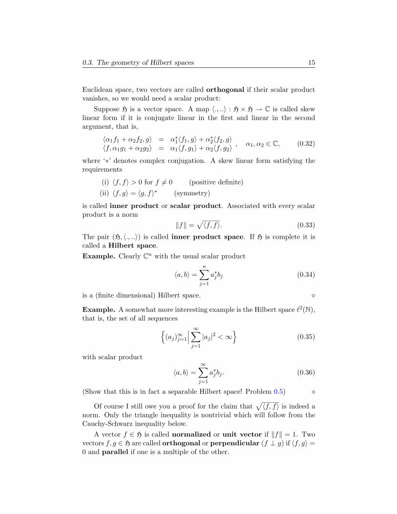
which is one line of computation.Suppose u is a unit vector, then the projection of f in the direction of
u is given byf‖ = 〈u, f〉u (0.38)
and f⊥ defined viaf⊥ = f − 〈u, f〉u (0.39)
is perpendicular to u since 〈u, f⊥〉 = 〈u, f−〈u, f〉u〉 = 〈u, f〉−〈u, f〉〈u, u〉 =0.
f
f‖
f⊥
u11B
BB
BBM
Taking any other vector parallel to u it is easy to see
‖f − αu‖2 = ‖f⊥ + (f‖ − αu)‖2 = ‖f⊥‖2 + |〈u, f〉 − α|2 (0.40)
and hence f‖ = 〈u, f〉u is the unique vector parallel to u which is closest tof .
As a first consequence we obtain the Cauchy-Schwarz-Bunjakowskiinequality:
Theorem 0.16 (Cauchy-Schwarz-Bunjakowski). Let H0 be an inner productspace, then for every f, g ∈ H0 we have
|〈f, g〉| ≤ ‖f‖ ‖g‖ (0.41)
with equality if and only if f and g are parallel.
Proof. It suffices to prove the case ‖g‖ = 1. But then the claim followsfrom ‖f‖2 = |〈g, f〉|2 + ‖f⊥‖2.
Note that the Cauchy-Schwarz inequality entails that the scalar productis continuous in both variables, that is, if fn → f and gn → g we have〈fn, gn〉 → 〈f, g〉.
As another consequence we infer that the map ‖.‖ is indeed a norm.
‖f + g‖2 = ‖f‖2 + 〈f, g〉+ 〈g, f〉+ ‖g‖2 ≤ (‖f‖+ ‖g‖)2. (0.42)
But let us return to C(I). Can we find a scalar product which has themaximum norm as associated norm? Unfortunately the answer is no! The
0.3. The geometry of Hilbert spaces 17
reason is that the maximum norm does not satisfy the parallelogram law(Problem 0.7).
Theorem 0.17 (Jordan-von Neumann). A norm is associated with a scalarproduct if and only if the parallelogram law
‖f + g‖2 + ‖f − g‖2 = 2‖f‖2 + 2‖g‖2 (0.43)
holds.In this case the scalar product can be recovered from its norm by virtue
of the polarization identity
〈f, g〉 =14(‖f + g‖2 − ‖f − g‖2 + i‖f − ig‖2 − i‖f + ig‖2
). (0.44)
Proof. If an inner product space is given, verification of the parallelogramlaw and the polarization identity is straight forward (Problem 0.6).
To show the converse, we define
s(f, g) =14(‖f + g‖2 − ‖f − g‖2 + i‖f − ig‖2 − i‖f + ig‖2
). (0.45)
Then s(f, f) = ‖f‖2 and s(f, g) = s(g, f)∗ are straightforward to check.Moreover, another straightforward computation using the parallelogram lawshows
s(f, g) + s(f, h) = 2s(f,g + h
2). (0.46)
Now choosing h = 0 (and using s(f, 0) = 0) shows s(f, g) = 2s(f, g2) andthus s(f, g) + s(f, h) = s(f, g + h). Furthermore, by induction we inferm2n s(f, g) = s(f, m2n g), that is λs(f, g) = s(f, λg) for every positive rational λ.By continuity (check this!) this holds for all λ > 0 and s(f,−g) = −s(f, g)respectively s(f, ig) = i s(f, g) finishes the proof.
Note that the parallelogram law and the polarization identity even holdfor skew linear forms (Problem 0.6).
But how do we define a scalar product on C(I)? One possibility is
〈f, g〉 =∫ b
af∗(x)g(x)dx. (0.47)
The corresponding inner product space is denoted by L2cont(I). Note that
we have‖f‖ ≤
√|b− a|‖f‖∞ (0.48)
and hence the maximum norm is stronger than the L2cont norm.
Suppose we have two norms ‖.‖1 and ‖.‖2 on a space X. Then ‖.‖2 issaid to be stronger than ‖.‖1 if there is a constant m > 0 such that
‖f‖1 ≤ m‖f‖2. (0.49)
18 0. A first look at Banach and Hilbert spaces
It is straightforward to check that
Lemma 0.18. If ‖.‖2 is stronger than ‖.‖1, then any ‖.‖2 Cauchy sequenceis also a ‖.‖1 Cauchy sequence.
Hence if a function F : X → Y is continuous in (X, ‖.‖1) it is alsocontinuos in (X, ‖.‖2) and if a set is dense in (X, ‖.‖2) it is also dense in(X, ‖.‖1).
In particular, L2cont is separable. But is it also complete? Unfortunately
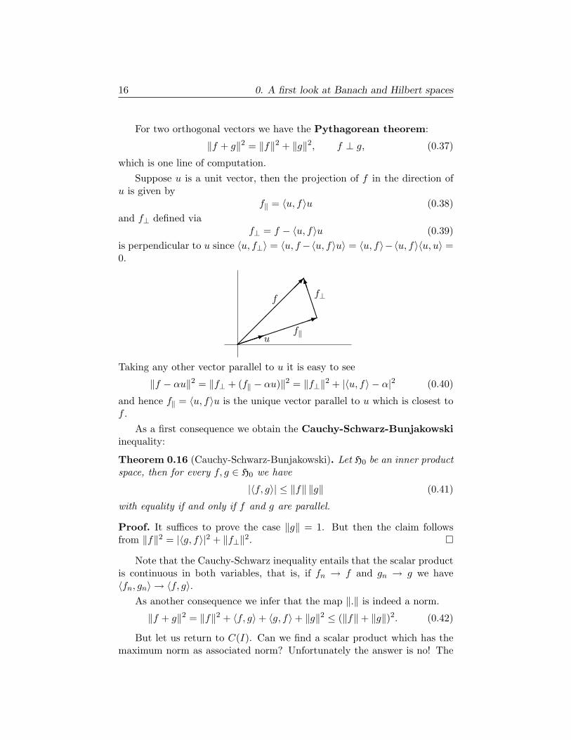
the answer is no:Example. Take I = [0, 2] and define
fn(x) =
0, 0 ≤ x ≤ 1− 1
n1 + n(x− 1), 1− 1
n ≤ x ≤ 11, 1 ≤ x ≤ 2
(0.50)
then fn(x) is a Cauchy sequence in L2cont, but there is no limit in L2
cont!Clearly the limit should be the step function which is 0 for 0 ≤ x < 1 and 1for 1 ≤ x ≤ 2, but this step function is discontinuous (Problem 0.8)!
This shows that in infinite dimensional spaces different norms will giveraise to different convergent sequences! In fact, the key to solving prob-lems in infinite dimensional spaces is often finding the right norm! This issomething which cannot happen in the finite dimensional case.
Theorem 0.19. If X is a finite dimensional case, then all norms are equiv-alent. That is, for given two norms ‖.‖1 and ‖.‖2 there are constants m1
and m2 such that1m2
‖f‖1 ≤ ‖f‖2 ≤ m1‖f‖1. (0.51)
Proof. Clearly we can choose a basis uj , 1 ≤ j ≤ n, and assume that ‖.‖2 isthe usual Euclidean norm, ‖
∑j αjuj‖2
2 =∑
j |αj |2. Let f =∑
j αjuj , thenby the triangle and Cauchy Schwartz inequalities
‖f‖1 ≤∑j
|αj |‖uj‖1 ≤√∑
j
‖uj‖21‖f‖2 (0.52)
and we can choose m2 =√∑
j ‖uj‖1.
In particular, if fn is convergent with respect to ‖.‖2 it is also convergentwith respect to ‖.‖1. Thus ‖.‖1 is continuous with respect to ‖.‖2 and attainsits minimum m > 0 on the unit sphere (which is compact by the Heine-Boreltheorem). Now choose m1 = 1/m.
Problem 0.5. Show that `2(N) is a separable Hilbert space.
0.4. Completeness 19
Problem 0.6. Let s(f, g) be a skew linear form and p(f) = s(f, f) theassociated quadratic form. Prove the parallelogram law
p(f + g) + p(f − g) = 2p(f) + 2p(g) (0.53)
and the polarization identity
s(f, g) =14
(p(f + g)− p(f − g) + i p(f − ig)− i p(f + ig)) . (0.54)
Problem 0.7. Show that the maximum norm (on C[0, 1]) does not satisfythe parallelogram law.
Problem 0.8. Prove the claims made about fn, defined in (0.50), in thelast example.
0.4. Completeness
Since L2cont is not complete, how can we obtain a Hilbert space out of it?
Well the answer is simple: take the completion.If X is a (incomplete) normed space, consider the set of all Cauchy
sequences X. Call two Cauchy sequences equivalent if their difference con-verges to zero and denote by X the set of all equivalence classes. It is easyto see that X (and X) inherit the vector space structure from X. Moreover,
Lemma 0.20. If xn is a Cauchy sequence, then ‖xn‖ converges.
Consequently the norm of a Cauchy sequence (xn)∞n=1 can be defined by‖(xn)∞n=1‖ = limn→∞ ‖xn‖ and is independent of the equivalence class (showthis!). Thus X is a normed space (X is not! why?).
Theorem 0.21. X is a Banach space containing X as a dense subspace ifwe identify x ∈ X with the equivalence class of all sequences converging tox.
Proof. (Outline) It remains to show that X is complete. Let ξn = [(xn,j)∞j=1]be a Cauchy sequence in X. Then it is not hard to see that ξ = [(xj,j)∞j=1]is its limit.
Let me remark that the completion X is unique. More precisely anyother complete space which contains X as a dense subset is isomorphic toX. This can for example be seen by showing that the identity map on Xhas a unique extension to X (compare Theorem 0.24 below).
In particular it is no restriction to assume that a normed linear spaceor an inner product space is complete. However, in the important caseof L2
cont it is somewhat inconvenient to work with equivalence classes ofCauchy sequences and hence we will give a different characterization usingthe Lebesgue integral later.
20 0. A first look at Banach and Hilbert spaces
0.5. Bounded operators
A linear map A between two normed spaces X and Y will be called a (lin-ear) operator
A : D(A) ⊆ X → Y. (0.55)
The linear subspace D(A) on which A is defined, is called the domain of Aand is usually required to be dense. The kernel
Ker(A) = f ∈ D(A)|Af = 0 (0.56)
and rangeRan(A) = Af |f ∈ D(A) = AD(A) (0.57)
are defined as usual. The operator A is called bounded if the followingoperator norm
‖A‖ = sup‖f‖X=1
‖Af‖Y (0.58)
is finite.The set of all bounded linear operators from X to Y is denoted by
L(X,Y ). If X = Y we write L(X,X) = L(X).
Theorem 0.22. The space L(X,Y ) together with the operator norm (0.58)is a normed space. It is a Banach space if Y is.
Proof. That (0.58) is indeed a norm is straightforward. If Y is complete andAn is a Cauchy sequence of operators, then Anf converges to an elementg for every f . Define a new operator A via Af = g. By continuity ofthe vector operations, A is linear and by continuity of the norm ‖Af‖ =limn→∞ ‖Anf‖ ≤ (limn→∞ ‖An‖)‖f‖ it is bounded. Furthermore, givenε > 0 there is some N such that ‖An − Am‖ ≤ ε for n,m ≥ N and thus‖Anf−Amf‖ ≤ ε‖f‖. Taking the limit m→∞ we see ‖Anf−Af‖ ≤ ε‖f‖,that is An → A.
By construction, a bounded operator is Lipschitz continuous
‖Af‖Y ≤ ‖A‖‖f‖X (0.59)
and hence continuous. The converse is also true
Theorem 0.23. An operator A is bounded if and only if it is continuous.
Proof. Suppose A is continuous but not bounded. Then there is a sequenceof unit vectors un such that ‖Aun‖ ≥ n. Then fn = 1
nun converges to 0 but‖Afn‖ ≥ 1 does not converge to 0.
Moreover, if A is bounded and densely defined, it is no restriction toassume that it is defined on all of X.
0.5. Bounded operators 21
Theorem 0.24. Let A ∈ L(X,Y ) and let Y be a Banach space. If D(A)is dense, there is a unique (continuous) extension of A to X, which has thesame norm.
Proof. Since a bounded operator maps Cauchy sequences to Cauchy se-quences, this extension can only be given by
Af = limn→∞
Afn, fn ∈ D(A), f ∈ X. (0.60)
To show that this definition is independent of the sequence fn → f , letgn → f be a second sequence and observe
‖Afn −Agn‖ = ‖A(fn − gn)‖ ≤ ‖A‖‖fn − gn‖ → 0. (0.61)
From continuity of vector addition and scalar multiplication it follows thatour extension is linear. Finally, from continuity of the norm we concludethat the norm does not increase.
An operator in L(X,C) is called a bounded linear functional and thespace X∗ = L(X,C) is called the dual space of X. A sequence fn is said toconverge weakly fn f if `(fn) → `(f) for every ` ∈ X∗.
The Banach space of bounded linear operators L(X) even has a multi-plication given by composition. Clearly this multiplication satisfies
(A+B)C = AC +BC, A(B+C) = AB+BC, A,B,C ∈ L(X) (0.62)
and
(AB)C = A(BC), α (AB) = (αA)B = A (αB), α ∈ C. (0.63)
Moreover, it is easy to see that we have
‖AB‖ ≤ ‖A‖‖B‖. (0.64)
However, note that our multiplication is not commutative (unless X is onedimensional). We even have an identity, the identity operator I satisfying‖I‖ = 1.
A Banach space together with a multiplication satisfying the above re-quirements is called a Banach algebra. In particular, note that (0.64)ensures that multiplication is continuous.
Problem 0.9. Show that the integral operator
(Kf)(x) =∫ 1
0K(x, y)f(y)dy, (0.65)
where K(x, y) ∈ C([0, 1] × [0, 1]), defined on D(K) = C[0, 1] is a boundedoperator both in X = C[0, 1] (max norm) and X = L2
cont(0, 1).
Problem 0.10. Show that the differential operator A = ddx defined on
D(A) = C1[0, 1] ⊂ C[0, 1] is an unbounded operator.
22 0. A first look at Banach and Hilbert spaces
Problem 0.11. Show that ‖AB‖ ≤ ‖A‖‖B‖ for every A,B ∈ L(X).
Problem 0.12. Show that the multiplication in a Banach algebra X is con-tinuous: xn → x and yn → y implies xnyn → xy.
0.6. Lebesgue Lp spaces
We fix some measure space (X,Σ, µ) and define the Lp norm by
‖f‖p =(∫
X|f |p dµ
)1/p
, 1 ≤ p (0.66)
and denote by Lp(X, dµ) the set of all complex valued measurable functionsfor which ‖f‖p is finite. First of all note that Lp(X, dµ) is a linear space,since |f + g|p ≤ 2p max(|f |, |g|)p ≤ 2p max(|f |p, |g|p) ≤ 2p(|f |p + |g|p). Ofcourse our hope is that Lp(X, dµ) is a Banach space. However, there isa small technical problem (recall that a property is said to hold almosteverywhere if the set where it fails to hold is contained in a set of measurezero):
Lemma 0.25. Let f be measurable, then∫X|f |p dµ = 0 (0.67)
if and only if f(x) = 0 almost everywhere with respect to µ.
Proof. Observe that we have A = x|f(x) 6= 0 =⋂nAn, where An =
x| |f(x)| > 1n. If
∫|f |pdµ = 0 we must have µ(An) = 0 for every n and
hence µ(A) = limn→∞ µ(An) = 0. The converse is obvious.
Note that the proof also shows that if f is not 0 almost everywhere,there is an ε > 0 such that µ(x| |f(x)| ≥ ε) > 0.Example. Let λ be the Lebesgue measure on R. Then the characteristicfunction of the rationals χQ is zero a.e. (with respect to λ). Let Θ be theDirac measure centered at 0, then f(x) = 0 a.e. (with respect to Θ) if andonly if f(0) = 0.
Thus ‖f‖p = 0 only implies f(x) = 0 for almost every x, but not for all!Hence ‖.‖p is not a norm on Lp(X, dµ). The way out of this misery is toidentify functions which are equal almost everywhere: Let
N (X, dµ) = f |f(x) = 0 µ-almost everywhere. (0.68)
Then N (X, dµ) is a linear subspace of Lp(X, dµ) and we can consider thequotient space
Lp(X, dµ) = Lp(X, dµ)/N (X, dµ). (0.69)
0.6. Lebesgue Lp spaces 23
If dµ is the Lebesgue measure on X ⊆ Rn we simply write Lp(X). Observethat ‖f‖p is well defined on Lp(X, dµ).
Even though the elements of Lp(X, dµ) are strictly speaking equivalenceclasses of functions, we will still call them functions for notational conve-nience. However, note that for f ∈ Lp(X, dµ) the value f(x) is not welldefined (unless there is a continuous representative and different continuousfunctions are in different equivalence classes, e.g., in the case of Lebesguemeasure).
With this modification we are back in business since Lp(X, dµ) turnsout to be a Banach space. We will show this in the following sections.
But before that let us also define L∞(X, dµ). It should be the set ofbounded measurable functions B(X) together with the sup norm. The onlyproblem is that if we want to identify functions equal almost everywhere, thesupremum is no longer independent of the equivalence class. The solutionis the essential supremum
‖f‖∞ = infC |µ(x| |f(x)| > C) = 0. (0.70)
That is, C is an essential bound if |f(x)| ≤ C almost everywhere and theessential supremum is the infimum over all essential bounds.Example. If λ is the Lebesgue measure, then the essential sup of χQ withrespect to λ is 0. If Θ is the Dirac measure centered at 0, then the essentialsup of χQ with respect to Θ is 1 (since χQ(0) = 1, and x = 0 is the onlypoint which counts for Θ).
As before we set
L∞(X, dµ) = B(X)/N (X, dµ) (0.71)
and observe that ‖f‖∞ is independent of the equivalence class.If you wonder where the ∞ comes from, have a look at Problem 0.13.As a preparation for proving that Lp is a Banach space, we will need
Holder’s inequality, which plays a central role in the theory of Lp spaces.In particular, it will imply Minkowski’s inequality, which is just the triangleinequality for Lp.
Theorem 0.26 (Holder’s inequality). Let p and q be dual indices, that is,
1p
+1q
= 1 (0.72)
with 1 ≤ p ≤ ∞. If f ∈ Lp(X, dµ) and g ∈ Lq(X, dµ) then fg ∈ L1(X, dµ)and
‖f g‖1 ≤ ‖f‖p‖g‖q. (0.73)
24 0. A first look at Banach and Hilbert spaces
Proof. The case p = 1, q = ∞ (respectively p = ∞, q = 1) follows directlyfrom the properties of the integral and hence it remains to consider 1 <p, q <∞.
First of all it is no restriction to assume ‖f‖p = ‖g‖q = 1. Then, usingthe elementary inequality (Problem 0.14)
a1/pb1/q ≤ 1pa+
1qb, a, b ≥ 0, (0.74)
with a = |f |p and b = |g|q and integrating over X gives∫X|f g|dµ ≤ 1
p
∫X|f |pdµ+
1q
∫X|g|qdµ = 1 (0.75)
and finishes the proof.
As a consequence we also get
Theorem 0.27 (Minkowski’s inequality). Let f, g ∈ Lp(X, dµ), then
‖f + g‖p ≤ ‖f‖p + ‖g‖p. (0.76)
Proof. Since the cases p = 1,∞ are straightforward, we only consider 1 <p <∞. Using |f+g|p ≤ |f | |f+g|p−1+ |g| |f+g|p−1 we obtain from Holder’sinequality (note (p− 1)q = p)
‖f + g‖pp ≤ ‖f‖p‖(f + g)p−1‖q + ‖g‖p‖(f + g)p−1‖q= (‖f‖p + ‖g‖p)‖(f + g)‖p−1
p . (0.77)
This shows that Lp(X, dµ) is a normed linear space. Finally it remainsto show that Lp(X, dµ) is complete.
Theorem 0.28. The space Lp(X, dµ) is a Banach space.
Proof. Suppose fn is a Cauchy sequence. It suffices to show that somesubsequence converges (show this). Hence we can drop some terms suchthat
‖fn+1 − fn‖p ≤12n. (0.78)
Now consider gn = fn − fn−1 (set f0 = 0). Then
G(x) =∞∑k=1
|gk(x)| (0.79)
is in Lp. This follows from∥∥∥ n∑k=1
|gk|∥∥∥p≤
n∑k=1
‖gk(x)‖p ≤ ‖f1‖p +12
(0.80)
0.6. Lebesgue Lp spaces 25
using the monotone convergence theorem. In particular, G(x) < ∞ almosteverywhere and the sum
∞∑n=1
gn(x) = limn→∞
fn(x) (0.81)
is absolutely convergent for those x. Now let f(x) be this limit. Since|f(x) − fn(x)|p converges to zero almost everywhere and |f(x) − fn(x)|p ≤2pG(x)p ∈ L1, dominated convergence shows ‖f − fn‖p → 0.
In particular, in the proof of the last theorem we have seen:
Corollary 0.29. If ‖fn − f‖p → 0 then there is a subsequence which con-verges pointwise almost everywhere.
It even turns out that Lp is separable.
Lemma 0.30. Suppose X is a second countable topological space (i.e., ithas a countable basis) and µ is a regular Borel measure. Then Lp(X, dµ),1 ≤ p <∞ is separable.
Proof. The set of all characteristic functions χA(x) with A ∈ Σ and µ(A) <∞, is total by construction of the integral. Now our strategy is as follows:Using outer regularity we can restrict A to open sets and using the existenceof a countable base, we can restrict A to open sets from this base.
Fix A. By outer regularity, there is a decreasing sequence of open setsOn such that µ(On) → µ(A). Since µ(A) <∞ it is no restriction to assumeµ(On) < ∞, and thus µ(On\A) = µ(On) − µ(A) → 0. Now dominatedconvergence implies ‖χA − χOn‖p → 0. Thus the set of all characteristicfunctions χO(x) with O open and µ(O) < ∞, is total. Finally let B be acountable basis for the topology. Then, every open set O can be written asO =
⋃∞j=1 Oj with Oj ∈ B. Moreover, by considering the set of all finite
unions of elements from B it is no restriction to assume⋃nj=1 Oj ∈ B. Hence
there is an increasing sequence On O with On ∈ B. By monotone con-vergence, ‖χO − χOn
‖p → 0 and hence the set of all characteristic functionsχO with O ∈ B is total.
To finish this chapter, let us show that continuous functions are densein Lp.
Theorem 0.31. Let X be a locally compact metric space and let µ be aσ-finite regular Borel measure. Then the set Cc(X) of continuous functionswith compact support is dense in Lp(X, dµ), 1 ≤ p <∞.
Proof. As in the previous proof the set of all characteristic functions χK(x)with K compact is total (using inner regularity). Hence it suffices to show
26 0. A first look at Banach and Hilbert spaces
that χK(x) can be approximated by continuous functions. By outer regu-larity there is an open set O ⊃ K such that µ(O\K) ≤ ε. By Urysohn’slemma (Lemma 0.11) there is a continuous function fε which is one on Kand 0 outside O. Since∫
X|χK − fε|pdµ =
∫O\K
|fε|pdµ ≤ µ(O\K) ≤ ε (0.82)
we have ‖fε − χK‖ → 0 and we are done.
If X is some subset of Rn we can do even better.A nonnegative function u ∈ C∞c (Rn) is called a mollifier if∫
Rn
u(x)dx = 1 (0.83)
The standard mollifier is u(x) = exp( 1|x|2−1
) for |x| < 1 and u(x) = 0 else.
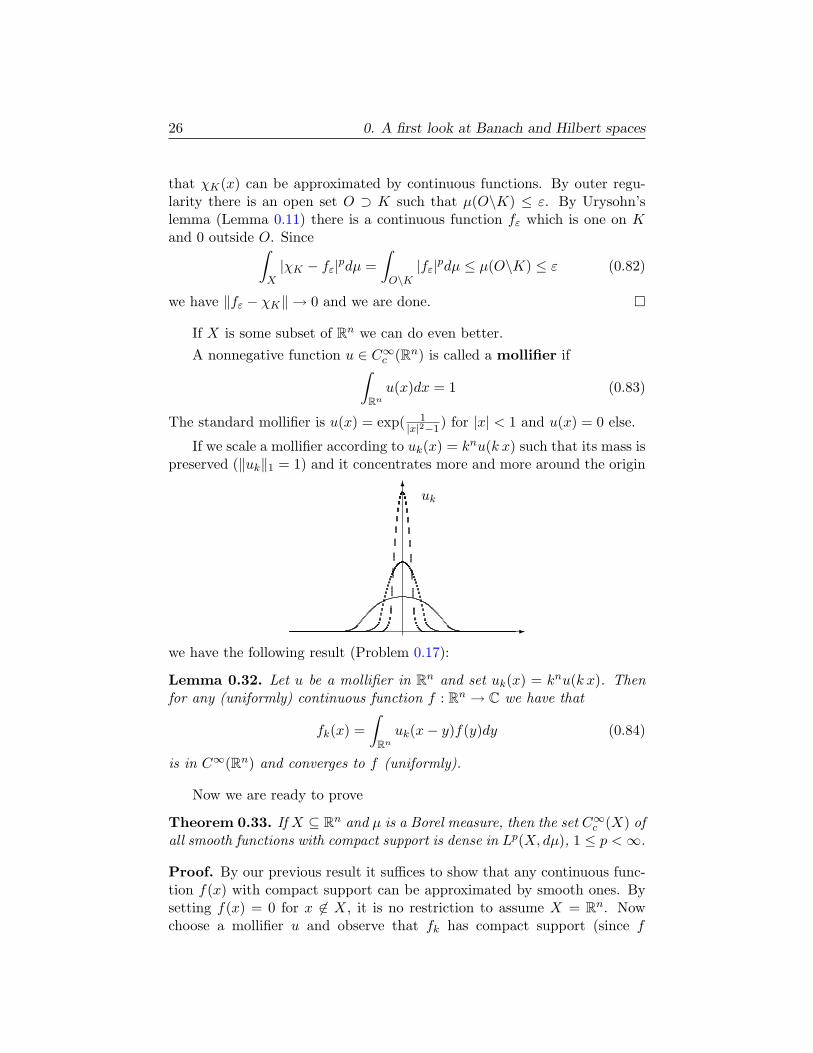
If we scale a mollifier according to uk(x) = knu(k x) such that its mass ispreserved (‖uk‖1 = 1) and it concentrates more and more around the origin
-
6 uk
we have the following result (Problem 0.17):
Lemma 0.32. Let u be a mollifier in Rn and set uk(x) = knu(k x). Thenfor any (uniformly) continuous function f : Rn → C we have that
fk(x) =∫
Rn
uk(x− y)f(y)dy (0.84)
is in C∞(Rn) and converges to f (uniformly).
Now we are ready to prove
Theorem 0.33. If X ⊆ Rn and µ is a Borel measure, then the set C∞c (X) ofall smooth functions with compact support is dense in Lp(X, dµ), 1 ≤ p <∞.
Proof. By our previous result it suffices to show that any continuous func-tion f(x) with compact support can be approximated by smooth ones. Bysetting f(x) = 0 for x 6∈ X, it is no restriction to assume X = Rn. Nowchoose a mollifier u and observe that fk has compact support (since f
0.7. Appendix: The uniform boundedness principle 27
has). Moreover, since f has compact support it is uniformly continuousand fk → f uniformly. But this implies fk → f in Lp.
Problem 0.13. Suppose µ(X) <∞. Show that
limp→∞
‖f‖p = ‖f‖∞ (0.85)
for any bounded measurable function.
Problem 0.14. Prove (0.74). (Hint: Show that f(x) = (1 − t) + tx − xt,x > 0, 0 < t < 1 satisfies f(a/b) ≥ 0 = f(1).)
Problem 0.15. Show the following generalization of Holder’s inequality
‖f g‖r ≤ ‖f‖p‖g‖q, (0.86)
where 1p + 1
q = 1r .
Problem 0.16 (Lyapunov inequality). Let 0 < θ < 1. Show that if f ∈Lp1 ∩ Lp2, then f ∈ Lp and
‖f‖p ≤ ‖f‖θp1‖f‖1−θp2 , (0.87)
where 1p = θ
p1+ 1−θ
p2.
Problem 0.17. Prove Lemma 0.32. (Hint: To show that fk is smooth useProblem A.7 and A.8.)
Problem 0.18. Construct a function f ∈ Lp(0, 1) which has a pole at everyrational number in [0, 1]. (Hint: Start with the function f0(x) = |x|−α whichhas a single pole at 0, then fj(x) = f0(x− xj) has a pole at xj.)
0.7. Appendix: The uniform boundednessprinciple
Recall that the interior of a set is the largest open subset (that is, the unionof all open subsets). A set is called nowhere dense if its closure has emptyinterior. The key to several important theorems about Banach spaces is theobservation that a Banach space cannot be the countable union of nowheredense sets.
Theorem 0.34 (Baire category theorem). Let X be a complete metric space,then X cannot be the countable union of nowhere dense sets.
Proof. Suppose X =⋃∞n=1Xn. We can assume that the sets Xn are closed
and none of them contains a ball, that is, X\Xn is open and nonempty forevery n. We will construct a Cauchy sequence xn which stays away from allXn.
28 0. A first look at Banach and Hilbert spaces
Since X\X1 is open and nonempty there is a closed ball Br1(x1) ⊆X\X1. Reducing r1 a little, we can even assume Br1(x1) ⊆ X\X1. More-over, since X2 cannot contain Br1(x1) there is some x2 ∈ Br1(x1) that isnot in X2. Since Br1(x1) ∩ (X\X2) is open there is a closed ball Br2(x2) ⊆Br1(x1) ∩ (X\X2). Proceeding by induction we obtain a sequence of ballssuch that
Brn(xn) ⊆ Brn−1(xn−1) ∩ (X\Xn). (0.88)Now observe that in every step we can choose rn as small as we please, hencewithout loss of generality rn → 0. Since by construction xn ∈ BrN (xN ) forn ≥ N , we conclude that xn is Cauchy and converges to some point x ∈ X.But x ∈ Brn(xn) ⊆ X\Xn for every n, contradicting our assumption thatthe Xn cover X.
(Sets which can be written as countable union of nowhere dense sets arecalled of first category. All other sets are second category. Hence the namecategory theorem.)
In other words, if Xn ⊆ X is a sequence of closed subsets which coverX, at least one Xn contains a ball of radius ε > 0.
Now we come to the first important consequence, the uniform bound-edness principle.
Theorem 0.35 (Banach-Steinhaus). Let X be a Banach space and Y somenormed linear space. Let Aα ⊆ L(X,Y ) be a family of bounded operators.Suppose ‖Aαx‖ ≤ C(x) is bounded for fixed x ∈ X, then ‖Aα‖ ≤ C isuniformly bounded.
Proof. Let
Xn = x| ‖Aαx‖ ≤ n for all α =⋂α
x| ‖Aαx‖ ≤ n, (0.89)
then⋃nXn = X by assumption. Moreover, by continuity of Aα and the
norm, each Xn is an intersection of closed sets and hence closed. By Baire’stheorem at least one contains a ball of positive radius: Bε(x0) ⊂ Xn. Nowobserve
‖Aαy‖ ≤ ‖Aα(y + x0)‖+ ‖Aαx0‖ ≤ n+ ‖Aαx0‖ (0.90)for ‖y‖ < ε. Setting y = ε x
‖x‖ we obtain
‖Aαx‖ ≤n+ C(x0)
ε‖x‖ (0.91)
for any x.
Part 1
MathematicalFoundations ofQuantum Mechanics

Chapter 1
Hilbert spaces
The phase space in classical mechanics is the Euclidean space R2n (for the nposition and n momentum coordinates). In quantum mechanics the phasespace is always a Hilbert space H. Hence the geometry of Hilbert spacesstands at the outset of our investigations.
1.1. Hilbert spaces
Suppose H is a vector space. A map 〈., ..〉 : H × H → C is called skewlinear form if it is conjugate linear in the first and linear in the secondargument. A positive definite skew linear form is called inner product orscalar product. Associated with every scalar product is a norm
‖ψ‖ =√〈ψ,ψ〉. (1.1)
The triangle inequality follows from the Cauchy-Schwarz-Bunjakowskiinequality:
|〈ψ,ϕ〉| ≤ ‖ψ‖ ‖ϕ‖ (1.2)
with equality if and only if ψ and ϕ are parallel.If H is complete with respect to the above norm, it is called a Hilbert
space. It is no restriction to assume that H is complete since one can easilyreplace it by its completion.Example. The space L2(M,dµ) is a Hilbert space with scalar product givenby
〈f, g〉 =∫Mf(x)∗g(x)dµ(x). (1.3)
31
32 1. Hilbert spaces
Similarly, the set of all square summable sequences `2(N) is a Hilbert spacewith scalar product
〈f, g〉 =∑j∈N
f∗j gj . (1.4)
(Note that the second example is a special case of the first one; take M = Rand µ a sum of Dirac measures.)
A vector ψ ∈ H is called normalized or unit vector if ‖ψ‖ = 1. Twovectors ψ,ϕ ∈ H are called orthogonal or perpendicular (ψ ⊥ ϕ) if〈ψ,ϕ〉 = 0 and parallel if one is a multiple of the other. If ψ and ϕ areorthogonal we have the Pythagorean theorem:
‖ψ + ϕ‖2 = ‖ψ‖2 + ‖ϕ‖2, ψ ⊥ ϕ, (1.5)
which is straightforward to check.Suppose ϕ is a unit vector, then the projection of ψ in the direction of
ϕ is given by
ψ‖ = 〈ϕ,ψ〉ϕ (1.6)
and ψ⊥ defined via
ψ⊥ = ψ − 〈ϕ,ψ〉ϕ (1.7)
is perpendicular to ϕ.These results can also be generalized to more than one vector. A set
of vectors ϕj is called orthonormal set if 〈ϕj , ϕk〉 = 0 for j 6= k and〈ϕj , ϕj〉 = 1.
Lemma 1.1. Suppose ϕjnj=0 is an orthonormal set. Then every ψ ∈ H
can be written as
ψ = ψ‖ + ψ⊥, ψ‖ =n∑j=0
〈ϕj , ψ〉ϕj , (1.8)
where ψ‖ and ψ⊥ are orthogonal. Moreover, 〈ϕj , ψ⊥〉 = 0 for all 1 ≤ j ≤ n.In particular,
‖ψ‖2 =n∑j=0
|〈ϕj , ψ〉|2 + ‖ψ⊥‖2. (1.9)
Moreover, every ψ in the span of ϕjnj=0 satisfies
‖ψ − ψ‖ ≥ ‖ψ⊥‖ (1.10)
with equality holding if and only if ψ = ψ‖. In other words, ψ‖ is uniquelycharacterized as the vector in the span of ϕjnj=0 being closest to ψ.
1.2. Orthonormal bases 33
Proof. A straightforward calculation shows 〈ϕj , ψ − ψ‖〉 = 0 and hence ψ‖and ψ⊥ = ψ − ψ‖ are orthogonal. The formula for the norm follows byapplying (1.5) iteratively.
Now, fix a vector
ψ =n∑j=0
cjϕj . (1.11)
in the span of ϕjnj=0. Then one computes
‖ψ − ψ‖2 = ‖ψ‖ + ψ⊥ − ψ‖2 = ‖ψ⊥‖2 + ‖ψ‖ − ψ‖2
= ‖ψ⊥‖2 +n∑j=0
|cj − 〈ϕj , ψ〉|2 (1.12)
from which the last claim follows.
From (1.9) we obtain Bessel’s inequalityn∑j=0
|〈ϕj , ψ〉|2 ≤ ‖ψ‖2 (1.13)
with equality holding if and only if ψ lies in the span of ϕjnj=0.Recall that a scalar product can be recovered from its norm by virtue of
the polarization identity
〈ϕ,ψ〉 =14(‖ϕ+ ψ‖2 − ‖ϕ− ψ‖2 + i‖ϕ− iψ‖2 − i‖ϕ+ iψ‖2
). (1.14)
A bijective operator U ∈ L(H1,H2) is called unitary if U preservesscalar products:
〈Uϕ,Uψ〉2 = 〈ϕ,ψ〉1, ϕ, ψ ∈ H1. (1.15)
By the polarization identity this is the case if and only if U preserves norms:‖Uψ‖2 = ‖ψ‖1 for all ψ ∈ H1. The two Hilbert space H1 and H2 are calledunitarily equivalent in this case.
Problem 1.1. The operator S : `2(N) → `2(N), (a1, a2, a3 . . . ) 7→ (0, a1, a2, . . . )clearly satisfies ‖Ua‖ = ‖a‖. Is it unitary?
1.2. Orthonormal bases
Of course, since we cannot assume H to be a finite dimensional vector space,we need to generalize Lemma 1.1 to arbitrary orthonormal sets ϕjj∈J .We start by assuming that J is countable. Then Bessel’s inequality (1.13)shows that ∑
j∈J|〈ϕj , ψ〉|2 (1.16)
34 1. Hilbert spaces
converges absolutely. Moreover, for any finite subset K ⊂ J we have
‖∑j∈K
〈ϕj , ψ〉ϕj‖2 =∑j∈K
|〈ϕj , ψ〉|2 (1.17)
by the Pythagorean theorem and thus∑
j∈J〈ϕj , ψ〉ϕj is Cauchy if and onlyif∑
j∈J |〈ϕj , ψ〉|2 is. Now let J be arbitrary. Again, Bessel’s inequalityshows that for any given ε > 0 there are at most finitely many j for which|〈ϕj , ψ〉| ≥ ε. Hence there are at most countably many j for which |〈ϕj , ψ〉| >0. Thus it follows that ∑
j∈J|〈ϕj , ψ〉|2 (1.18)
is well-defined and so is ∑j∈J
〈ϕj , ψ〉ϕj . (1.19)
In particular, by continuity of the scalar product we see that Lemma 1.1holds for arbitrary orthonormal sets without modifications.
Theorem 1.2. Suppose ϕjj∈J is an orthonormal set. Then every ψ ∈ H
can be written as
ψ = ψ‖ + ψ⊥, ψ‖ =∑j∈J
〈ϕj , ψ〉ϕj , (1.20)
where ψ‖ and ψ⊥ are orthogonal. Moreover, 〈ϕj , ψ⊥〉 = 0 for all j ∈ J . Inparticular,
‖ψ‖2 =∑j∈J
|〈ϕj , ψ〉|2 + ‖ψ⊥‖2. (1.21)
Moreover, every ψ in the span of ϕjj∈J satisfies
‖ψ − ψ‖ ≥ ‖ψ⊥‖ (1.22)
with equality holding if and only if ψ = ψ‖. In other words, ψ‖ is uniquelycharacterized as the vector in the span of ϕjj∈J being closest to ψ.
Note that from Bessel’s inequality (which of course still holds) it followsthat the map ψ → ψ‖ is continuous.
An orthonormal set which is not a proper subset of any other orthonor-mal set is called an orthonormal basis due to following result:
Theorem 1.3. For an orthonormal set ϕjj∈J the following conditions areequivalent:(i) ϕjj∈J is a maximal orthonormal set.(ii) For every vector ψ ∈ H we have
ψ =∑j∈J
〈ϕj , ψ〉ϕj . (1.23)
1.2. Orthonormal bases 35
(iii) For every vector ψ ∈ H we have
‖ψ‖2 =∑j∈J
|〈ϕj , ψ〉|2. (1.24)
(iv) 〈ϕj , ψ〉 = 0 for all j ∈ J implies ψ = 0.
Proof. We will use the notation from Theorem 1.2.(i) ⇒ (ii): If ψ⊥ 6= 0 than we can normalize ψ⊥ to obtain a unit vector ψ⊥which is orthogonal to all vectors ϕj . But then ϕjj∈J ∪ ψ⊥ would be alarger orthonormal set, contradicting maximality of ϕjj∈J .(ii) ⇒ (iii): Follows since (ii) implies ψ⊥ = 0.(iii) ⇒ (iv): If 〈ψ,ϕj〉 = 0 for all j ∈ J we conclude ‖ψ‖2 = 0 and henceψ = 0.(iv) ⇒ (i): If ϕjj∈J were not maximal, there would be a unit vector ϕsuch that ϕjj∈J ∪ ϕ is larger orthonormal set. But 〈ϕj , ϕ〉 = 0 for allj ∈ J implies ϕ = 0 by (iv), a contradiction.
Since ψ → ψ‖ is continuous, it suffices to check conditions (ii) and (iii)on a dense set.Example. The set of functions
ϕn(x) =1√2π
einx, n ∈ Z, (1.25)
forms an orthonormal basis for H = L2(0, 2π). The corresponding orthogo-nal expansion is just the ordinary Fourier series. (Problem 1.17)
A Hilbert space is separable if and only if there is a countable orthonor-mal basis. In fact, if H is separable, then there exists a countable total setψjNj=0. After throwing away some vectors we can assume that ψn+1 can-not be expressed as a linear combinations of the vectors ψ0, . . .ψn. Now wecan construct an orthonormal basis as follows: We begin by normalizing ψ0
ϕ0 =ψ0
‖ψ0‖. (1.26)
Next we take ψ1 and remove the component parallel to ϕ0 and normalizeagain
ϕ1 =ψ1 − 〈ϕ0, ψ1〉ϕ0
‖ψ1 − 〈ϕ0, ψ1〉ϕ0‖. (1.27)
Proceeding like this we define recursively
ϕn =ψn −
∑n−1j=0 〈ϕj , ψn〉ϕj
‖ψn −∑n−1
j=0 〈ϕj , ψn〉ϕj‖. (1.28)
This procedure is known as Gram-Schmidt orthogonalization. Hencewe obtain an orthonormal set ϕjNj=0 such that spanϕjnj=0 = spanψjnj=0
36 1. Hilbert spaces
for any finite n and thus also for N . Since ψjNj=0 is total, we infer thatϕjNj=0 is an orthonormal basis.
Example. In L2(−1, 1) we can orthogonalize the polynomial fn(x) = xn.The resulting polynomials are up to a normalization equal to the Legendrepolynomials
P0(x) = 1, P1(x) = x, P2(x) =3x2 − 1
2, . . . (1.29)
(which are normalized such that Pn(1) = 1).
If fact, if there is one countable basis, then it follows that any other basisis countable as well.
Theorem 1.4. If H is separable, then every orthonormal basis is countable.
Proof. We know that there is at least one countable orthonormal basisϕjj∈J . Now let φkk∈K be a second basis and consider the set Kj =k ∈ K|〈φk, ϕj〉 6= 0. Since these are the expansion coefficients of ϕj withrespect to φkk∈K , this set is countable. Hence the set K =
⋃j∈J Kj is
countable as well. But k ∈ K\K implies φk = 0 and hence K = K.
We will assume all Hilbert spaces to be separable.
In particular, it can be shown that L2(M,dµ) is separable. Moreover, itturns out that, up to unitary equivalence, there is only one (separable)infinite dimensional Hilbert space:
Let H be an infinite dimensional Hilbert space and let ϕjj∈N be anyorthogonal basis. Then the map U : H → `2(N), ψ 7→ (〈ϕj , ψ〉)j∈N is unitary(by Theorem 1.3 (iii)). In particular,
Theorem 1.5. Any separable infinite dimensional Hilbert space is unitarilyequivalent to `2(N).
Let me remark that if H is not separable, there still exists an orthonor-mal basis. However, the proof requires Zorn’s lemma: The collection ofall orthonormal sets in H can be partially ordered by inclusion. Moreover,any linearly ordered chain has an upper bound (the union of all sets in thechain). Hence Zorn’s lemma implies the existence of a maximal element,that is, an orthonormal basis.
1.3. The projection theorem and the Rieszlemma
Let M ⊆ H be a subset, then M⊥ = ψ|〈ϕ,ψ〉 = 0, ∀ϕ ∈ M is calledthe orthogonal complement of M . By continuity of the scalar prod-uct it follows that M⊥ is a closed linear subspace and by linearity that
1.3. The projection theorem and the Riesz lemma 37
(span(M))⊥ = M⊥. For example we have H⊥ = 0 since any vector in H⊥
must be in particular orthogonal to all vectors in some orthonormal basis.
Theorem 1.6 (projection theorem). Let M be a closed linear subspace of aHilbert space H, then every ψ ∈ H can be uniquely written as ψ = ψ‖ + ψ⊥with ψ‖ ∈M and ψ⊥ ∈M⊥. One writes
M ⊕M⊥ = H (1.30)
in this situation.
Proof. Since M is closed, it is a Hilbert space and has an orthonormal basisϕjj∈J . Hence the result follows from Theorem 1.2.
In other words, to every ψ ∈ H we can assign a unique vector ψ‖ whichis the vector in M closest to ψ. The rest ψ − ψ‖ lies in M⊥. The operatorPMψ = ψ‖ is called the orthogonal projection corresponding to M . Notethat we have
P 2M = PM and 〈PMψ,ϕ〉 = 〈ψ, PMϕ〉 (1.31)
since 〈PMψ,ϕ〉 = 〈ψ‖, ϕ‖〉 = 〈ψ, PMϕ〉. Clearly we have PM⊥ψ = ψ −PMψ = ψ⊥.
Moreover, we see that the vectors in a closed subspace M are preciselythose which are orthogonal to all vectors in M⊥, that is, M⊥⊥ = M . If Mis an arbitrary subset we have at least
M⊥⊥ = span(M). (1.32)
Note that by H⊥ = we see that M⊥ = 0 if and only if M is dense.Finally we turn to linear functionals, that is, to operators ` : H →
C. By the Cauchy-Schwarz inequality we know that `ϕ : ψ 7→ 〈ϕ,ψ〉 is abounded linear functional (with norm ‖ϕ‖). In turns out that in a Hilbertspace every bounded linear functional can be written in this way.
Theorem 1.7 (Riesz lemma). Suppose ` is a bounded linear functional ona Hilbert space H. Then there is a vector ϕ ∈ H such that `(ψ) = 〈ϕ,ψ〉 forall ψ ∈ H. In other words, a Hilbert space is equivalent to its own dual spaceH∗ = H.
Proof. If ` ≡ 0 we can choose ϕ = 0. Otherwise Ker(`) = ψ|`(ψ) = 0is a proper subspace and we can find a unit vector ϕ ∈ Ker(`)⊥. For everyψ ∈ H we have `(ψ)ϕ− `(ϕ)ψ ∈ Ker(`) and hence
0 = 〈ϕ, `(ψ)ϕ− `(ϕ)ψ〉 = `(ψ)− `(ϕ)〈ϕ, ψ〉. (1.33)
In other words, we can choose ϕ = `(ϕ)∗ϕ.
The following easy consequence is left as an exercise.
38 1. Hilbert spaces
Corollary 1.8. Suppose B is a bounded skew liner form, that is,
|B(ψ,ϕ)| ≤ C‖ψ‖ ‖ϕ‖. (1.34)
Then there is a unique bounded operator A such that
B(ψ,ϕ) = 〈Aψ,ϕ〉. (1.35)
Problem 1.2. Show that an orthogonal projection PM 6= 0 has norm one.
Problem 1.3. Suppose P1 and P1 are orthogonal projections. Show thatP1 ≤ P2 (that is 〈ψ, P1ψ〉 ≤ 〈ψ, P2ψ〉) is equivalent to Ran(P1) ⊆ Ran(P2).
Problem 1.4. Prove Corollary 1.8.
Problem 1.5. Let ϕj be some orthonormal basis. Show that a boundedlinear operator A is uniquely determined by its matrix elements Ajk =〈ϕj , Aϕk〉 with respect to this basis.
Problem 1.6. Show that L(H) is not separable H is infinite dimensional.
Problem 1.7. Show P : L2(R) → L2(R), f(x) 7→ 12(f(x) + f(−x)) is a
projection. Compute its range and kernel.
1.4. Orthogonal sums and tensor products
Given two Hilbert spaces H1 and H2 we define their orthogonal sum H1⊕H2
to be the set of all pairs (ψ1, ψ2) ∈ H1×H2 together with the scalar product
〈(ϕ1, ϕ2), (ψ1, ψ2)〉 = 〈ϕ1, ψ1〉1 + 〈ϕ2, ψ2〉2. (1.36)
It is left as an exercise to verify that H1 ⊕ H2 is again a Hilbert space.Moreover, H1 can be identified with (ψ1, 0)|ψ1 ∈ H1 and we can regardH1 as a subspace of H1 ⊕ H2. Similarly for H2. It is also custom to writeψ1 + ψ2 instead of (ψ1, ψ2).
More generally, let Hj j ∈ N, be a countable collection of Hilbert spacesand define
∞⊕j=1
Hj = ∞∑j=1
ψj |ψj ∈ Hj ,∞∑j=1
‖ψj‖2j <∞, (1.37)
which becomes a Hilbert space with the scalar product
〈∞∑j=1
ϕj ,∞∑j=1
ψj〉 =∞∑j=1
〈ϕj , ψj〉j . (1.38)
Suppose H and H are two Hilbert spaces. Our goal is to construct theirtensor product. The elements should be products ψ ⊗ ψ of elements ψ ∈ H
1.4. Orthogonal sums and tensor products 39
and ψ ∈ H. Hence we start with the set of all finite linear combinations ofelements of H× H
F(H, H) = n∑j=1
αj(ψj , ψj)|(ψj , ψj) ∈ H× H, αj ∈ C. (1.39)
Since we want (ψ1+ψ2)⊗ψ = ψ1⊗ψ+ψ2⊗ψ, ψ⊗(ψ1+ψ2) = ψ⊗ψ1+ψ⊗ψ2,and (αψ)⊗ ψ = ψ ⊗ (αψ) we consider F(H, H)/N (H, H), where
N (H, H) = spann∑
j,k=1
αjβk(ψj , ψk)− (n∑j=1
αjψj ,
n∑k=1
βkψk) (1.40)
and write ψ ⊗ ψ for the equivalence class of (ψ, ψ).Next we define
〈ψ ⊗ ψ, φ⊗ φ〉 = 〈ψ, φ〉〈ψ, φ〉 (1.41)which extends to a skew linear form on F(H, H)/N (H, H). To show that weobtain a scalar product, we need to ensure positivity. Let ψ =
∑i αiψi⊗ψi 6=
0 and pick orthonormal bases ϕj , ϕk for spanψi, spanψi, respectively.Then
ψ =∑j,k
αjkϕj ⊗ ϕk, αjk =∑i
αi〈ϕj , ψi〉〈ϕk, ψi〉 (1.42)
and we compute〈ψ,ψ〉 =
∑j,k
|αjk|2 > 0. (1.43)
The completion of F(H, H)/N (H, H) with respect to the induced norm iscalled the tensor product H⊗ H of H and H.
Lemma 1.9. If ϕj, ϕk are orthonormal bases for H, H, respectively, thenϕj ⊗ ϕk is an orthonormal basis for H⊗ H.
Proof. That ϕj⊗ ϕk is an orthonormal set is immediate from (1.41). More-over, since spanϕj, spanϕk is dense in H, H, respectively, it is easy tosee that ϕj ⊗ ϕk is dense in F(H, H)/N (H, H). But the latter is dense inH⊗ H.
Example. We have H⊗ Cn = Hn.
Example. Let (M,dµ) and (M, dµ) be two measure spaces. Then we haveL2(M,dµ)⊗ L2(M, dµ) = L2(M × M, dµ× dµ).
Clearly we have L2(M,dµ) ⊗ L2(M, dµ) ⊆ L2(M × M, dµ × dµ). Nowtake an orthonormal basis ϕj ⊗ ϕk for L2(M,dµ) ⊗ L2(M, dµ) as in ourprevious lemma. Then∫
M
∫M
(ϕj(x)ϕk(y))∗f(x, y)dµ(x)dµ(y) = 0 (1.44)
40 1. Hilbert spaces
implies∫Mϕj(x)∗fk(x)dµ(x) = 0, fk(x) =
∫Mϕk(y)∗f(x, y)dµ(y) (1.45)
and hence fk(x) = 0 µ-a.e. x. But this implies f(x, y) = 0 for µ-a.e. x andµ-a.e. y and thus f = 0. Hence ϕj ⊗ ϕk is a basis for L2(M × M, dµ× dµ)and equality follows.
It is straightforward to extend the tensor product to any finite numberof Hilbert spaces. We even note
(∞⊕j=1
Hj)⊗ H =∞⊕j=1
(Hj ⊗ H), (1.46)
where equality has to be understood in the sense, that both spaces areunitarily equivalent by virtue of the identification
(∞∑j=1
ψj)⊗ ψ =∞∑j=1
ψj ⊗ ψ. (1.47)
Problem 1.8. We have ψ⊗ψ = φ⊗φ if and only if there is some α ∈ C\0such that ψ = αφ and ψ = α−1φ.
Problem 1.9. Show (1.46)
1.5. The C∗ algebra of bounded linear operators
We start by introducing a conjugation for operators on a Hilbert space H.Let A = L(H), then the adjoint operator is defined via
〈ϕ,A∗ψ〉 = 〈Aϕ,ψ〉 (1.48)
(compare Corollary 1.8).Example. If H = Cn and A = (ajk)1≤j,k≤n, then A∗ = (a∗kj)1≤j,k≤n.
Lemma 1.10. Let A,B ∈ L(H), then
(i) (A+B)∗ = A∗ +B∗, (αA)∗ = α∗A∗,
(ii) A∗∗ = A,
(iii) (AB)∗ = B∗A∗,
(iv) ‖A‖ = ‖A∗‖ and ‖A‖2 = ‖A∗A‖ = ‖AA∗‖.
Proof. (i) and (ii) are obvious. (iii) follows from 〈ϕ, (AB)ψ〉 = 〈A∗ϕ,Bψ〉 =〈B∗A∗ϕ,ψ〉. (iv) follows from
‖A∗‖ = sup‖ϕ‖=‖ψ‖=1
|〈ψ,A∗ϕ〉| = sup‖ϕ‖=‖ψ‖=1
|〈Aψ,ϕ〉| = ‖A‖. (1.49)
1.6. Weak and strong convergence 41
and
‖A∗A‖ = sup‖ϕ‖=‖ψ‖=1
|〈ϕ,A∗Aψ〉| = sup‖ϕ‖=‖ψ‖=1
|〈Aϕ,Aψ〉|
= sup‖ϕ‖=1
‖Aϕ‖2 = ‖A‖2, (1.50)
where we have used ‖ϕ‖ = sup‖ψ‖=1 |〈ψ,ϕ〉|.
As a consequence of ‖A∗‖ = ‖A‖ observe that taking the adjoint iscontinuous.
In general, a Banach algebra A together with an involution
(a+ b)∗ = a∗ + b∗, (αa)∗ = α∗a∗, a∗∗ = a, (ab)∗ = b∗a∗, (1.51)
satisfying‖a‖2 = ‖a∗a‖ (1.52)
is called a C∗ algebra. The element a∗ is called the adjoint of a. Note that‖a∗‖ = ‖a‖ follows from (1.52) and ‖aa∗‖ ≤ ‖a‖‖a∗‖.
Any subalgebra which is also closed under involution, is called a ∗-algebra. An ideal is a subspace I ⊆ A such that a ∈ I, b ∈ A impliesab ∈ I and ba ∈ I. If it is closed under the adjoint map it is called a ∗-ideal.Note that if there is and identity e we have e∗ = e and hence (a−1)∗ = (a∗)−1
(show this).Example. The continuous function C(I) together with complex conjuga-tion form a commutative C∗ algebra.
An element a ∈ A is called normal if aa∗ = a∗a, self-adjoint if a = a∗,unitary if aa∗ = a∗a = I, (orthogonal) projection if a = a∗ = a2, andpositive if a = bb∗ for some b ∈ A. Clearly both self-adjoint and unitaryelements are normal.
Problem 1.10. Let A ∈ L(H). Show that A is normal if and only if
‖Aψ‖ = ‖A∗ψ‖, ∀ψ ∈ H. (1.53)
(Hint: Problem 0.6)
Problem 1.11. Show that U : H → H is unitary if and only if U−1 = U∗.
Problem 1.12. Compute the adjoint of S : `2(N) → `2(N), (a1, a2, a3 . . . ) 7→(0, a1, a2, . . . ).
1.6. Weak and strong convergence
Sometimes a weaker notion of convergence is useful: We say that ψn con-verges weakly to ψ and write
w-limn→∞
ψn = ψ or ψn ψ. (1.54)
42 1. Hilbert spaces
if 〈ϕ,ψn〉 → 〈ϕ,ψ〉 for every ϕ ∈ H (show that a weak limit is unique).Example. Let ϕn be an (infinite) orthonormal set. Then 〈ψ,ϕn〉 → 0 forevery ψ since these are just the expansion coefficients of ψ. (ϕn does notconverge to 0, since ‖ϕn‖ = 1.)
Clearly ψn → ψ implies ψn ψ and hence this notion of convergence isindeed weaker. Moreover, the weak limit is unique, since 〈ϕ,ψn〉 → 〈ϕ,ψ〉and 〈ϕ,ψn〉 → 〈ϕ, ψ〉 implies 〈ϕ, (ψ−ψ)〉 = 0. A sequence ψn is called weakCauchy sequence if 〈ϕ,ψn〉 is Cauchy for every ϕ ∈ H.
Lemma 1.11. Let H be a Hilbert space.
(i) ψn ψ implies ‖ψ‖ ≤ lim inf ‖ψn‖.(ii) Every weak Cauchy sequence ψn is bounded: ‖ψn‖ ≤ C.(iii) Every weak Cauchy sequence converges weakly.(iv) For a weakly convergent sequence ψn ψ we have: ψn → ψ if
and only if lim sup ‖ψn‖ ≤ ‖ψ‖.
Proof. (i) Observe
‖ψ‖2 = 〈ψ,ψ〉 = lim inf〈ψ,ψn〉 ≤ ‖ψ‖ lim inf ‖ψn‖. (1.55)
(ii) For every ϕ we have that |〈ϕ,ψn〉| ≤ C(ϕ) is bounded. Hence by theuniform boundedness principle we have ‖ψn‖ = ‖〈ψn, .〉‖ ≤ C.(iii) Let ϕm be an orthonormal basis and define cm = limn→∞〈ϕm, ψn〉.Then ψ =
∑m cmϕm is the desired limit.
(iv) By (i) we have lim ‖ψn‖ = ‖ψ‖ and hence
‖ψ − ψn‖2 = ‖ψ‖2 − 2Re(〈ψ,ψn〉) + ‖ψn‖2 → 0. (1.56)
The converse is straightforward.
Clearly an orthonormal basis does not have a norm convergent subse-quence. Hence the unit ball in an infinite dimensional Hilbert space is nevercompact. However, we can at least extract weakly convergent subsequences:
Lemma 1.12. Let H be a Hilbert space. Every bounded sequence ψn hasweakly convergent subsequence.
Proof. Let ϕk be an ONB, then by the usual diagonal sequence argumentwe can find a subsequence ψnm such that 〈ϕk, ψnm〉 converges for all k. Sinceψn is bounded, 〈ϕ,ψnm〉 converges for every ϕ ∈ H and hence ψnm is a weakCauchy sequence.
Finally, let me remark that similar concepts can be introduced for oper-ators. This is of particular importance for the case of unbounded operators,where convergence in the operator norm makes no sense at all.
1.6. Weak and strong convergence 43
A sequence of operators An is said to converge strongly to A,
s-limn→∞
An = A :⇔ Anψ → Aψ ∀x ∈ D(A) ⊆ D(An). (1.57)
It is said to converge weakly to A,
w-limn→∞
An = A :⇔ Anψ Aψ ∀ψ ∈ D(A) ⊆ D(An). (1.58)
Clearly norm convergence implies strong convergence and strong conver-gence implies weak convergence.Example. Consider the operator Sn ∈ L(`2(N)) which shifts a sequence nplaces to the left
Sn (x1, x2, . . . ) = (xn+1, xn+2, . . . ). (1.59)
and the operator S∗n ∈ L(`2(N)) which shifts a sequence n places to the rightand fills up the first n places with zeros
S∗n (x1, x2, . . . ) = (0, . . . , 0︸ ︷︷ ︸n places
, x1, x2, . . . ). (1.60)
Then Sn converges to zero strongly but not in norm and S∗n converges weaklyto zero but not strongly.
Note that this example also shows that taking adjoints is not continuouswith respect to strong convergence! If An
s→ A we only have
〈ϕ,A∗nψ〉 = 〈Anϕ,ψ〉 → 〈Aϕ,ψ〉 = 〈ϕ,A∗ψ〉 (1.61)
and hence A∗n A∗ in general. However, if An and A are normal we have
‖(An −A)∗ψ‖ = ‖(An −A)ψ‖ (1.62)
and hence A∗ns→ A∗ in this case. Thus at least for normal operators taking
adjoints is continuous with respect to strong convergence.
Lemma 1.13. Suppose An is a sequence of bounded operators.
(i) s-limn→∞An = A implies ‖A‖ ≤ lim inf ‖An‖.(ii) Every strong Cauchy sequence An is bounded: ‖An‖ ≤ C.
(iii) If Any → Ay for y in a dense set and ‖An‖ ≤ C, than s-limn→∞An =A.
The same result holds if strong convergence is replaced by weak convergence.
Proof. (i) and (ii) follow as in Lemma 1.11 (i).(ii) Just use
‖Anψ −Aψ‖ ≤ ‖Anψ −Anϕ‖+ ‖Anϕ−Aϕ‖+ ‖Aϕ−Aψ‖≤ 2C‖ψ − ϕ‖+ ‖Anϕ−Aϕ‖ (1.63)
44 1. Hilbert spaces
and choose ϕ in the dense subspace such that ‖ψ − ϕ‖ ≤ ε4C and n large
such that ‖Anϕ−Aϕ‖ ≤ ε2 .
The case of weak convergence is left as an exercise.
Problem 1.13. Suppose ψn → ψ and ϕn ϕ. Then 〈ψn, ϕn〉 → 〈ψ,ϕ〉.
Problem 1.14. Let ϕj be some orthonormal basis. Show that ψn ϕif and only if ψn is bounded and 〈ϕj , ψn〉 → 〈ϕj , ψ〉 for every j. Show thatthis is wrong without the boundedness assumption.
Problem 1.15. Let ϕj∞j=1 be some orthonormal basis and define
‖ψ‖w =∞∑j=1
12j|〈ϕj , ψ〉|. (1.64)
Show that ‖.‖w is a norm. Show that ψn ϕ if and only if ‖ψn−ψ‖w → 0.
Problem 1.16. A subspace M ⊆ H is closed if and only if every weakCauchy sequence in M has a limit in M . (Hint: M = M⊥⊥.)
1.7. Appendix: The Stone–Weierstraß theorem
In case of a self-adjoint operator, the spectral theorem will show that theclosed ∗-algebra generated by this operator is isomorphic to the C∗ algebraof continuous functions C(K) over some compact set. Hence it is importantto be able to identify dense sets:
Theorem 1.14 (Stone–Weierstraß, real version). Suppose K is a compactset and let C(K,R) be the Banach algebra of continuous functions (with thesup norm).
If F ⊂ C(K,R) contains the identity 1 and separates points (i.e., forevery x1 6= x2 there is some function f ∈ F such that f(x1) 6= f(x2)), thenthe algebra generated by F is dense.
Proof. Denote by A the algebra generated by F . Note that if f ∈ A,we have |f | ∈ A: By the Weierstraß approximation theorem (Theorem 0.13)there is a polynomial pn(t) such that
∣∣|t|−pn(t)∣∣ < 1n and hence pn(f) → |f |.
In particular, if f, g in A, we also have
maxf, g =(f + g) + |f − g|
2, minf, g =
(f + g)− |f − g|2
(1.65)
in A.Now fix f ∈ C(K,R). We need to find some fε ∈ A with ‖f − fε‖∞ < ε.First of all, since A separates points, observe that for given y, z ∈ K
there is a function fy,z ∈ A such that fy,z(y) = f(y) and fy,z(z) = f(z)
1.7. Appendix: The Stone–Weierstraß theorem 45
(show this). Next, for every y ∈ K there is a neighborhood U(y) such that
fy,z(x) > f(x)− ε, x ∈ U(y) (1.66)
and since K is compact, finitely many, say U(y1), . . . U(yj), cover K. Then
fz = maxfy1,z, . . . , fyj ,z ∈ A (1.67)
and satisfies fz > f − ε by construction. Since fz(z) = f(z) for every z ∈ Kthere is a neighborhood V (z) such that
fz(x) < f(x) + ε, x ∈ V (z) (1.68)
and a corresponding finite cover V (z1), . . . V (zk). Now
fε = minfz1 , . . . , fzk ∈ A (1.69)
satisfies fε < f + ε. Since f − ε < fzl< fε, we have found a required
function.
Theorem 1.15 (Stone–Weierstraß). Suppose K is a compact set and letC(K) be the C∗ algebra of continuous functions (with the sup norm).
If F ⊂ C(K) contains the identity 1 and separates points, then the ∗-algebra generated by F is dense.
Proof. Just observe that F = Re(f), Im(f)|f ∈ F satisfies the assump-tion of the real version. Hence any real-valued continuous functions can beapproximated by elements from F , in particular this holds for the real andimaginary part for any given complex-valued function.
Note that the additional requirement of being closed under complexconjugation is crucial: The functions holomorphic on the unit ball and con-tinuous on the boundary separate points, but they are not dense (since theuniform limit of holomorphic functions is again holomorphic).
Corollary 1.16. Suppose K is a compact set and let C(K) be the C∗ algebraof continuous functions (with the sup norm).
If F ⊂ C(K) separates points, then the closure of the ∗-algebra generatedby F is either C(K) or f ∈ C(K)|f(t0) = 0 for some t0 ∈ K.
Proof. There are two possibilities, either all f ∈ F vanish at one pointt0 ∈ K (there can be at most one such point since F separates points)or there is no such point. If there is no such point we can proceed as inthe proof of the Stone–Weierstraß theorem to show that the identity canbe approximated by elements in A (note that to show |f | ∈ A if f ∈ Awe do not need the identity, since pn can be chosen to contain no constantterm). If there is such a t0, the identity is clearly missing from A. However,adding the identity to A we get A + C = C(K) and it is easy to see thatA = f ∈ C(K)|f(t0) = 0.
46 1. Hilbert spaces
Problem 1.17. Show that the of functions ϕn(x) = 1√2π
einx, n ∈ Z, forman orthonormal basis for H = L2(0, 2π).
Problem 1.18. Show that the ∗-algebra generated by fz(t) = 1t−z , z ∈ C, is
dense in the C∗ algebra C∞(R) of continuous functions vanishing at infinity.(Hint: Add ∞ to R to make it compact.)
Chapter 2
Self-adjointness andspectrum
2.1. Some quantum mechanics
In quantum mechanics, a single particle living in R3 is described by acomplex-valued function (the wave function)
ψ(x, t), (x, t) ∈ R3 × R, (2.1)
where x corresponds to a point in space and t corresponds to time. Thequantity ρt(x) = |ψ(x, t)|2 is interpreted as the probability density of theparticle at the time t. In particular, ψ must be normalized according to∫
R3
|ψ(x, t)|2d3x = 1, t ∈ R. (2.2)
The location x of the particle is a quantity which can be observed (i.e.,measured) and is hence called observable. Due to our probabilistic inter-pretation it is also a random variable whose expectation is given by
Eψ(x) =∫
R3
x|ψ(x, t)|2d3x. (2.3)
In a real life setting, it will not be possible to measure x directly and one willonly be able to measure certain functions of x. For example, it is possible tocheck whether the particle is inside a certain area Ω of space (e.g., inside adetector). The corresponding observable is the characteristic function χΩ(x)of this set. In particular, the number
Eψ(χΩ) =∫
R3
χΩ(x)|ψ(x, t)|2d3x =∫
Ω|ψ(x, t)|2d3x (2.4)
47
48 2. Self-adjointness and spectrum
corresponds to the probability of finding the particle inside Ω ⊆ R3. Animportant point to observe is that, in contradistinction to classical mechan-ics, the particle is no longer localized at a certain point. In particular,the mean-square deviation (or variance) ∆ψ(x)2 = Eψ(x2) − Eψ(x)2 isalways nonzero.
In general, the configuration space (or phase space) of a quantumsystem is a (complex) Hilbert space H and the possible states of this systemare represented by the elements ψ having norm one, ‖ψ‖ = 1.
An observable a corresponds to a linear operator A in this Hilbert spaceand its expectation, if the system is in the state ψ, is given by the realnumber
Eψ(A) = 〈ψ,Aψ〉 = 〈Aψ,ψ〉, (2.5)
where 〈., ..〉 denotes the scalar product of H. Similarly, the mean-squaredeviation is given by
∆ψ(A)2 = Eψ(A2)− Eψ(A)2 = ‖(A− Eψ(A))ψ‖2. (2.6)
Note that ∆ψ(A) vanishes if and only if ψ is an eigenstate corresponding tothe eigenvalue Eψ(A), that is, Aψ = Eψ(A)ψ.
From a physical point of view, (2.5) should make sense for any ψ ∈ H.However, this is not in the cards as our simple example of one particle alreadyshows. In fact, the reader is invited to find a square integrable function ψ(x)for which xψ(x) is no longer square integrable. The deeper reason behindthis nuisance is that Eψ(x) can attain arbitrary large values if the particleis not confined to a finite domain, which renders the corresponding opera-tor unbounded. But unbounded operators cannot be defined on the entireHilbert space in a natural way by the closed graph theorem (Theorem 2.7below) .
Hence, A will only be defined on a subset D(A) ⊆ H called the domainof A. Since we want A to at least be defined for most states, we requireD(A) to be dense.
However, it should be noted that there is no general prescription how tofind the operator corresponding to a given observable.
Now let us turn to the time evolution of such a quantum mechanicalsystem. Given an initial state ψ(0) of the system, there should be a uniqueψ(t) representing the state of the system at time t ∈ R. We will write
ψ(t) = U(t)ψ(0). (2.7)
Moreover, it follows from physical experiments, that superposition ofstates holds, that is, U(t)(α1ψ1(0)+α2ψ2(0)) = α1ψ1(t)+α2ψ2(t) (|α1|2 +|α2|2 = 1). In other words, U(t) should be a linear operator. Moreover,
2.1. Some quantum mechanics 49
since ψ(t) is a state (i.e., ‖ψ(t)‖ = 1), we have
‖U(t)ψ‖ = ‖ψ‖. (2.8)
Such operators are called unitary. Next, since we have assumed uniquenessof solutions to the initial value problem, we must have
U(0) = I, U(t+ s) = U(t)U(s). (2.9)
A family of unitary operators U(t) having this property is called a one-parameter unitary group. In addition, it is natural to assume that thisgroup is strongly continuous
limt→t0
U(t)ψ = U(t0)ψ, ψ ∈ H. (2.10)
Each such group has an infinitesimal generator defined by
Hψ = limt→0
it(U(t)ψ − ψ), D(H) = ψ ∈ H| lim
t→0
1t(U(t)ψ − ψ) exists.
(2.11)This operator is called the Hamiltonian and corresponds to the energy ofthe system. If ψ(0) ∈ D(H), then ψ(t) is a solution of the Schrodingerequation (in suitable units)
id
dtψ(t) = Hψ(t). (2.12)
This equation will be the main subject of our course.In summary, we have the following axioms of quantum mechanics.
Axiom 1. The configuration space of a quantum system is a complexseparable Hilbert space H and the possible states of this system are repre-sented by the elements of H which have norm one.
Axiom 2. Each observable a corresponds to a linear operator A definedmaximally on a dense subset D(A). Moreover, the operator correspond-ing to a polynomial Pn(a) =
∑nj=0 αja
j , αj ∈ R, is Pn(A) =∑n
j=0 αjAj ,
D(Pn(A)) = D(An) = ψ ∈ D(A)|Aψ ∈ D(An−1) (A0 = I).Axiom 3. The expectation value for a measurement of a, when the
system is in the state ψ ∈ D(A), is given by (2.5), which must be real forall ψ ∈ D(A).
Axiom 4. The time evolution is given by a strongly continuous one-parameter unitary group U(t). The generator of this group corresponds tothe energy of the system.
In the following sections we will try to draw some mathematical conse-quences from these assumptions:
50 2. Self-adjointness and spectrum
First we will see that Axiom 2 and 3 imply that observables correspondto self-adjoint operators. Hence these operators play a central role in quan-tum mechanics and we will derive some of their basic properties. Anothercrucial role is played by the set of all possible expectation values for themeasurement of a, which is connected with the spectrum σ(A) of the corre-sponding operator A.
The problem of defining functions of an observable will lead us to thespectral theorem (in the next chapter), which generalizes the diagonalizationof symmetric matrices.
Axiom 4 will be the topic of Chapter 5.
2.2. Self-adjoint operators
Let H be a (complex separable) Hilbert space. A linear operator is a linearmapping
A : D(A) → H, (2.13)
where D(A) is a linear subspace of H, called the domain of A. It is calledbounded if the operator norm
‖A‖ = sup‖ψ‖=1
‖Aψ‖ = sup‖ϕ‖=‖ψ‖=1
|〈ψ,Aϕ〉| (2.14)
is finite. The second equality follows since equality in |〈ψ,Aϕ〉| ≤ ‖ψ‖ ‖Aϕ‖is attained when Aϕ = zψ for some z ∈ C. If A is bounded it is no restrictionto assume D(A) = H and we will always do so. The Banach space of allbounded linear operators is denoted by L(H).
The expression 〈ψ,Aψ〉 encountered in the previous section is called thequadratic form
qA(ψ) = 〈ψ,Aψ〉, ψ ∈ D(A), (2.15)
associated to A. An operator can be reconstructed from its quadratic formvia the polarization identity
〈ϕ,Aψ〉 =14
(qA(ϕ+ ψ)− qA(ϕ− ψ) + iqA(ϕ− iψ)− iqA(ϕ+ iψ)) . (2.16)
A densely defined linear operator A is called symmetric (or Hermitian)if
〈ϕ,Aψ〉 = 〈Aϕ,ψ〉, ψ, ϕ ∈ D(A). (2.17)
The justification for this definition is provided by the following
Lemma 2.1. A densely defined operator A is symmetric if and only if thecorresponding quadratic form is real-valued.
2.2. Self-adjoint operators 51
Proof. Clearly (2.17) implies that Im(qA(ψ)) = 0. Conversely, taking theimaginary part of the identity
qA(ψ + iϕ) = qA(ψ) + qA(ϕ) + i(〈ψ,Aϕ〉 − 〈ϕ,Aψ〉) (2.18)
shows Re〈Aϕ,ψ〉 = Re〈ϕ,Aψ〉. Replacing ϕ by iϕ in this last equationshows Im〈Aϕ,ψ〉 = Im〈ϕ,Aψ〉 and finishes the proof.
In other words, a densely defined operator A is symmetric if and only if
〈ψ,Aψ〉 = 〈Aψ,ψ〉, ψ ∈ D(A). (2.19)
This already narrows the class of admissible operators to the class ofsymmetric operators by Axiom 3. Next, let us tackle the issue of the correctdomain.
By Axiom 2, A should be defined maximally, that is, if A is anothersymmetric operator such that A ⊆ A, then A = A. Here we write A ⊆ A ifD(A) ⊆ D(A) and Aψ = Aψ for all ψ ∈ D(A). In addition, we write A = A
if both A ⊆ A and A ⊆ A hold.The adjoint operator A∗ of a densely defined linear operator A is
defined by
D(A∗) = ψ ∈ H|∃ψ ∈ H : 〈ψ,Aϕ〉 = 〈ψ, ϕ〉,∀ϕ ∈ D(A)A∗ψ = ψ
. (2.20)
The requirement that D(A) is dense implies that A∗ is well-defined. How-ever, note that D(A∗) might not be dense in general. In fact, it mightcontain no vectors other than 0.
Clearly we have (αA)∗ = α∗A∗ for α ∈ C and (A + B)∗ ⊇ A∗ + B∗
provided D(A + B) = D(A) ∩ D(B) is dense. However, equality will nothold in general unless one operator is bounded (Problem 2.1).
For later use, note that (Problem 2.2)
Ker(A∗) = Ran(A)⊥. (2.21)
For symmetric operators we clearly have A ⊆ A∗. If in addition, A = A∗
holds, then A is called self-adjoint. Our goal is to show that observablescorrespond to self-adjoint operators. This is for example true in the case ofthe position operator x, which is a special case of a multiplication operator.Example. (Multiplication operator) Consider the multiplication operator
(Af)(x) = A(x)f(x), D(A) = f ∈ L2(Rn, dµ) |Af ∈ L2(Rn, dµ),(2.22)
given by multiplication with the measurable function A : Rn → C. Firstof all note that D(A) is dense. In fact, consider Ωn = x ∈ Rn | |A(x)| ≤n Rn. Then, for every f ∈ L2(Rn, dµ) the function fn = χΩnf ∈ D(A)converges to f as n→∞ by dominated convergence.
52 2. Self-adjointness and spectrum
Next, let us compute the adjoint of A. Performing a formal computationwe have for h, f ∈ D(A) that
〈h,Af〉 =∫h(x)∗A(x)f(x)dµ(x) =
∫(A(x)∗h(x))∗f(x)dµ(x) = 〈Ah, f〉,
(2.23)where A is multiplication by A(x)∗,
(Af)(x) = A(x)∗f(x), D(A) = f ∈ L2(Rn, dµ) | Af ∈ L2(Rn, dµ).(2.24)
Note D(A) = D(A). At first sight this seems to show that the adjoint ofA is A. But for our calculation we had to assume h ∈ D(A) and theremight be some functions in D(A∗) which do not satisfy this requirement! Inparticular, our calculation only shows A ⊆ A∗. To show that equality holds,we need to work a little harder:
If h ∈ D(A∗) there is some g ∈ L2(Rn, dµ) such that∫h(x)∗A(x)f(x)dµ(x) =
∫g(x)∗f(x)dµ(x), f ∈ D(A), (2.25)
and thus∫(h(x)A(x)∗ − g(x))∗f(x)dµ(x) = 0, f ∈ D(A). (2.26)
In particular,∫χΩn(x)(h(x)A(x)∗ − g(x))∗f(x)dµ(x) = 0, f ∈ L2(Rn, dµ), (2.27)
which shows that χΩn(h(x)A(x)∗ − g(x))∗ ∈ L2(Rn, dµ) vanishes. Since nis arbitrary, we even have h(x)A(x)∗ = g(x) ∈ L2(Rn, dµ) and thus A∗ ismultiplication by A(x)∗ and D(A∗) = D(A).
In particular, A is self-adjoint if A is real-valued. In the general case wehave at least ‖Af‖ = ‖A∗f‖ for all f ∈ D(A) = D(A∗). Such operators arecalled normal.
Now note thatA ⊆ B ⇒ B∗ ⊆ A∗, (2.28)
that is, increasing the domain of A implies decreasing the domain of A∗.Thus there is no point in trying to extend the domain of a self-adjointoperator further. In fact, if A is self-adjoint and B is a symmetric extension,we infer A ⊆ B ⊆ B∗ ⊆ A∗ = A implying A = B.
Corollary 2.2. Self-adjoint operators are maximal, that is, they do not haveany symmetric extensions.
Furthermore, if A∗ is densely defined (which is the case if A is symmetric)we can consider A∗∗. From the definition (2.20) it is clear that A ⊆ A∗∗ and
2.2. Self-adjoint operators 53
thus A∗∗ is an extension of A. This extension is closely related to extendinga linear subspace M via M⊥⊥ = M (as we will see a bit later) and thus iscalled the closure A = A∗∗ of A.
If A is symmetric we have A ⊆ A∗ and hence A = A∗∗ ⊆ A∗, that is,A lies between A and A∗. Moreover, 〈ψ,A∗ϕ〉 = 〈Aψ,ϕ〉 for all ψ ∈ D(A),ϕ ∈ D(A∗) implies that A is symmetric since A∗ϕ = Aϕ for ϕ ∈ D(A).Example. (Differential operator) Take H = L2(0, 2π).
(i). Consider the operator
A0f = −id
dxf, D(A0) = f ∈ C1[0, 2π] | f(0) = f(2π) = 0. (2.29)
That A0 is symmetric can be shown by a simple integration by parts (dothis). Note that the boundary conditions f(0) = f(2π) = 0 are chosensuch that the boundary terms occurring from integration by parts vanish.However, this will also follow once we have computed A∗0. If g ∈ D(A∗0) wemust have ∫ 2π
0g(x)∗(−if ′(x))dx =
∫ 2π
0g(x)∗f(x)dx (2.30)
for some g ∈ L2(0, 2π). Integration by parts shows∫ 2π
0f ′(x)
(g(x)− i
∫ x
0g(t)dt
)∗dx = 0 (2.31)
and hence g(x) − i∫ x0 g(t)dt ∈ f ′|f ∈ D(A0)⊥. But f ′|f ∈ D(A0) =
h ∈ C(0, 2π)|∫ 2π0 h(t)dt = 0 implying g(x) = g(0) + i
∫ x0 g(t)dt since
f ′|f ∈ D(A0) = h ∈ H|〈1, h〉 = 0 = 1⊥ and 1⊥⊥ = span1. Thusg ∈ AC[0, 2π], where
AC[a, b] = f ∈ C[a, b]|f(x) = f(a) +∫ x
ag(t)dt, g ∈ L1(a, b) (2.32)
denotes the set of all absolutely continuous functions (see Section 2.6). Insummary, g ∈ D(A∗0) implies g ∈ AC[0, 2π] and A∗0g = g = −ig′. Conversely,for every g ∈ H1(0, 2π) = f ∈ AC[0, 2π]|f ′ ∈ L2(0, 2π) (2.30) holds withg = −ig′ and we conclude
A∗0f = −id
dxf, D(A∗0) = H1(0, 2π). (2.33)
In particular, A is symmetric but not self-adjoint. Since A∗∗ ⊆ A∗ wecompute
0 = 〈g,A0f〉 − 〈A∗0g, f〉 = i(f(0)g(0)∗ − f(2π)g(2π)∗) (2.34)
54 2. Self-adjointness and spectrum
and since the boundary values of g ∈ D(A∗0) can be prescribed arbitrary, wemust have f(0) = f(2π) = 0. Thus
A0f = −id
dxf, D(A0) = f ∈ D(A∗0) | f(0) = f(2π) = 0. (2.35)
(ii). Now let us take
Af = −id
dxf, D(A) = f ∈ C1[0, 2π] | f(0) = f(2π). (2.36)
which is clearly an extension of A0. Thus A∗ ⊆ A∗0 and we compute
0 = 〈g,Af〉 − 〈A∗g, f〉 = if(0)(g(0)∗ − g(2π)∗). (2.37)
Since this must hold for all f ∈ D(A) we conclude g(0) = g(2π) and
A∗f = −id
dxf, D(A∗) = f ∈ H1(0, 2π) | f(0) = f(2π). (2.38)
Similarly, as before, A = A∗ and thus A is self-adjoint.
One might suspect that there is no big difference between the two sym-metric operators A0 and A from the previous example, since they coincideon a dense set of vectors. However, the converse is true: For example, thefirst operator A0 has no eigenvectors at all (i.e., solutions of the equationA0ψ = zψ, z ∈ C) whereas the second one has an orthonormal basis ofeigenvectors!Example. Compute the eigenvectors of A0 and A from the previous exam-ple.
(i). By definition an eigenvector is a (nonzero) solution of A0u = zu,z ∈ C, that is, a solution of the ordinary differential equation
u′(x) = zu(x) (2.39)
satisfying the boundary conditions u(0) = u(2π) = 0 (since we must haveu ∈ D(A0). The general solution of the differential equation is u(x) =u(0)eizx and the boundary conditions imply u(x) = 0. Hence there are noeigenvectors.
(ii). Now we look for solutions of Au = zu, that is the same differentialequation as before, but now subject to the boundary condition u(0) = u(2π).Again the general solution is u(x) = u(0)eizx and the boundary conditionrequires u(0) = u(0)e2πiz. Thus there are two possibilities. Either u(0) = 0(which is of no use for us) or z ∈ Z. In particular, we see that all eigenvectorsare given by
un(x) =1√2π
einx, n ∈ Z, (2.40)
which are well-known to form an orthonormal basis.
2.2. Self-adjoint operators 55
We will see a bit later that this is a consequence of self-adjointness ofA. Hence it will be important to know whether a given operator is self-adjoint or not. Our example shows that symmetry is easy to check (in caseof differential operators it usually boils down to integration by parts), butcomputing the adjoint of an operator is a nontrivial job even in simple situ-ations. However, we will learn soon that self-adjointness is a much strongerproperty than symmetry justifying the additional effort needed to prove it.
On the other hand, if a given symmetric operator A turns out not tobe self-adjoint, this raises the question of self-adjoint extensions. Two casesneed to be distinguished. If A is self-adjoint, then there is only one self-adjoint extension (if B is another one, we have A ⊆ B and hence A = Bby Corollary 2.2). In this case A is called essentially self-adjoint andD(A) is called a core for A. Otherwise there might be more than one self-adjoint extension or none at all. This situation is more delicate and will beinvestigated in Section 2.5.
Since we have seen that computing A∗ is not always easy, a criterion forself-adjointness not involving A∗ will be useful.
Lemma 2.3. Let A be symmetric such that Ran(A+ z) = Ran(A+ z∗) = H
for one z ∈ C. Then A is self-adjoint.
Proof. Let ψ ∈ D(A∗) and A∗ψ = ψ. Since Ran(A + z∗) = H, there is aϑ ∈ D(A) such that (A+ z∗)ϑ = ψ + z∗ψ. Now we compute
〈ψ, (A+ z)ϕ〉 = 〈ψ+ z∗ψ,ϕ〉 = 〈(A+ z∗)ϑ, ϕ〉 = 〈ϑ, (A+ z)ϕ〉, ϕ ∈ D(A),(2.41)
and hence ψ = ϑ ∈ D(A) since Ran(A+ z) = H.
To proceed further, we will need more information on the closure ofan operator. We will use a different approach which avoids the use of theadjoint operator. We will establish equivalence with our original definitionin Lemma 2.4.
The simplest way of extending an operator A is to take the closure of itsgraph Γ(A) = (ψ,Aψ)|ψ ∈ D(A) ⊂ H2. That is, if (ψn, Aψn) → (ψ, ψ)we might try to define Aψ = ψ. For Aψ to be well-defined, we need that(ψn, Aψn) → (0, ψ) implies ψ = 0. In this case A is called closable and theunique operator A which satisfies Γ(A) = Γ(A) is called the closure of A.Clearly, A is called closed if A = A, which is the case if and only if thegraph of A is closed. Equivalently, A is closed if and only if Γ(A) equippedwith the graph norm ‖ψ‖2
Γ(A) = ‖ψ‖2 + ‖Aψ‖2 is a Hilbert space (i.e.,closed). A bounded operator is closed if and only if its domain is closed(show this!).
56 2. Self-adjointness and spectrum
Example. Let us compute the closure of the operator A0 from the pre-vious example without the use of the adjoint operator. Let f ∈ D(A0)and let fn ∈ D(A0) be a sequence such that fn → f , A0fn → −ig. Thenf ′n → g and hence f(x) =
∫ x0 g(t)dt. Thus f ∈ AC[0, 2π] and f(0) = 0.
Moreover f(2π) = limn→0
∫ 2π0 f ′n(t)dt = 0. Conversely, any such f can be
approximated by functions in D(A0) (show this).
Next, let us collect a few important results.
Lemma 2.4. Suppose A is a densely defined operator.
(i) A∗ is closed.
(ii) A is closable if and only if D(A∗) is dense and A = A∗∗ respectively(A)∗ = A∗ in this case.
(iii) If A is injective and the Ran(A) is dense, then (A∗)−1 = (A−1)∗.If A is closable and A is injective, then A
−1 = A−1.
Proof. Let us consider the following two unitary operators from H2 to itself
U(ϕ,ψ) = (ψ,−ϕ), V (ϕ,ψ) = (ψ,ϕ). (2.42)
(i). From
Γ(A∗) = (ϕ, ϕ) ∈ H2|〈ϕ,Aψ〉 = 〈ϕ, ψ〉 ∀ϕ ∈ D(A∗)= (ϕ, ϕ) ∈ H2|〈(−ϕ, ϕ), (ψ, ψ)〉Γ(A) = 0 ∀(ψ, ψ) ∈ Γ(A)= U(Γ(A)⊥) = (UΓ(A))⊥ (2.43)
we conclude that A∗ is closed.(ii). From
Γ(A) = Γ(A)⊥⊥ = (UΓ(A∗))⊥
= (ψ, ψ)| 〈ψ,A∗ϕ〉 − 〈ψ, ϕ〉 = 0,∀ϕ ∈ D(A∗) (2.44)
we see that (0, ψ) ∈ Γ(A) if and only if ψ ∈ D(A∗)⊥. Hence A is closable ifand only if D(A∗) is dense. In this case, equation (2.43) also shows A∗ = A∗.Moreover, replacing A by A∗ in (2.43) and comparing with the last formulashows A∗∗ = A.
(iii). Next note that (provided A is injective)
Γ(A−1) = V Γ(A). (2.45)
Hence if Ran(A) is dense, then Ker(A∗) = Ran(A)⊥ = 0 and
Γ((A∗)−1) = V Γ(A∗) = V UΓ(A)⊥ = UV Γ(A)⊥ = U(V Γ(A))⊥ (2.46)
2.2. Self-adjoint operators 57
shows that (A∗)−1 = (A−1)∗. Similarly, if A is closable and A is injective,then A−1 = A−1 by
Γ(A−1) = V Γ(A) = V Γ(A) = Γ(A−1). (2.47)
If A ∈ L(H) we clearly have D(A∗) = H and by Corollary 1.8 A ∈ L(H).In particular, since A = A∗∗ we obtain
Theorem 2.5. We have A ∈ L(H) if and only if A∗ ∈ L(H).
Now we can also generalize Lemma 2.3 to the case of essential self-adjointoperators.
Lemma 2.6. A symmetric operator A is essentially self-adjoint if and onlyif one of the following conditions holds for one z ∈ C\R.
• Ran(A+ z) = Ran(A+ z∗) = H.
• Ker(A∗ + z) = Ker(A∗ + z∗) = 0.
If A is non-negative, that is 〈ψ,Aψ〉 ≥ 0 for all ψ ∈ D(A), we can alsoadmit z ∈ (−∞, 0).
Proof. As noted earlier Ker(A∗) = Ran(A)⊥, and hence the two conditionsare equivalent. By taking the closure of A it is no restriction to assume thatA is closed. Let z = x+ iy. From
‖(A−z)ψ‖2 = ‖(A−x)ψ− iyψ‖2 = ‖(A−x)ψ‖2+y2‖ψ‖2 ≥ y2‖ψ‖2, (2.48)
we infer that Ker(A−z) = 0 and hence (A−z)−1 exists. Moreover, settingψ = (A − z)−1ϕ (y 6= 0) shows ‖(A − z)−1‖ ≤ |y|−1. Hence (A − z)−1 isbounded and closed. Since it is densely defined by assumption, its domainRan(A+ z) must be equal to H. Replacing z by z∗ and applying Lemma 2.3finishes the general case. The argument for the non-negative case withz < 0 is similar using ε‖ψ‖2 ≤ |〈ψ, (A + ε)ψ〉|2 ≤ ‖ψ‖‖(A + ε)ψ‖ whichshows (A+ ε)−1 ≤ ε−1, ε > 0.
In addition, we can also prove the closed graph theorem which showsthat an unbounded operator cannot be defined on the entire Hilbert space.
Theorem 2.7 (closed graph). Let H1 and H2 be two Hilbert spaces and Aan operator defined on all of H1. Then A is bounded if and only if Γ(A) isclosed.
Proof. If A is bounded than it is easy to see that Γ(A) is closed. So let usassume that Γ(A) is closed. Then A∗ is well defined and for all unit vectors
58 2. Self-adjointness and spectrum
ϕ ∈ D(A∗) we have that the linear functional `ϕ(ψ) = 〈A∗ϕ,ψ〉 is pointwisebounded
‖`ϕ(ψ)‖ = |〈ϕ,Aψ〉| ≤ ‖Aψ‖. (2.49)Hence by the uniform boundedness principle there is a constant C such that‖`ϕ‖ = ‖A∗ϕ‖ ≤ C. That is, A∗ is bounded and so is A = A∗∗.
Finally we want to draw some some further consequences of Axiom 2and show that observables correspond to self-adjoint operators. Since self-adjoint operators are already maximal, the difficult part remaining is toshow that an observable has at least one self-adjoint extension. There is agood way of doing this for non-negative operators and hence we will considerthis case first.
An operator is called non-negative (resp. positive) if 〈ψ,Aψ〉 ≥ 0(resp. > 0 for ψ 6= 0) for all ψ ∈ D(A). If A is positive, the map (ϕ,ψ) 7→〈ϕ,Aψ〉 is a scalar product. However, there might be sequences which areCauchy with respect to this scalar product but not with respect to ouroriginal one. To avoid this, we introduce the scalar product
〈ϕ,ψ〉A = 〈ϕ, (A+ 1)ψ〉, A ≥ 0, (2.50)
defined on D(A), which satisfies ‖ψ‖ ≤ ‖ψ‖A. Let HA be the completion ofD(A) with respect to the above scalar product. We claim that HA can beregarded as a subspace of H, that is, D(A) ⊆ HA ⊆ H.
If (ψn) is a Cauchy sequence in D(A), then it is also Cauchy in H (since‖ψ‖ ≤ ‖ψ‖A by assumption) and hence we can identify it with the limit of(ψn) regarded as a sequence in H. For this identification to be unique, weneed to show that if (ψn) ⊂ D(A) is a Cauchy sequence in HA such that‖ψn‖ → 0, then ‖ψn‖A → 0. This follows from
‖ψn‖2A = 〈ψn, ψn − ψm〉A + 〈ψn, ψm〉A
≤ ‖ψn‖A‖ψn − ψm‖A + ‖ψn‖‖(A+ 1)ψm‖ (2.51)
since the right hand side can be made arbitrarily small choosing m,n large.Clearly the quadratic form qA can be extended to every ψ ∈ HA by
settingqA(ψ) = 〈ψ,ψ〉A − ‖ψ‖2, ψ ∈ Q(A) = HA. (2.52)
The set Q(A) is also called the form domain of A.Example. (Multiplication operator) Let A be multiplication by A(x) ≥ 0in L2(Rn, dµ). Then
Q(A) = D(A1/2) = f ∈ L2(Rn, dµ) |A1/2f ∈ L2(Rn, dµ) (2.53)
andqA(x) =
∫Rn
A(x)|f(x)|2dµ(x) (2.54)
2.2. Self-adjoint operators 59
(show this).
Now we come to our extension result. Note that A + 1 is injective andthe best we can hope for is that for a non-negative extension A, A+ 1 is abijection from D(A) onto H.
Lemma 2.8. Suppose A is a non-negative operator, then there is a non-negative extension A such that Ran(A+ 1) = H.
Proof. Let us define an operator A by
D(A) = ψ ∈ HA|∃ψ ∈ H : 〈ϕ,ψ〉A = 〈ϕ, ψ〉,∀ϕ ∈ HAAψ = ψ − ψ
. (2.55)
Since HA is dense, ψ is well-defined. Moreover, it is straightforward to seethat A is a non-negative extension of A.
It is also not hard to see that Ran(A+ 1) = H. Indeed, for any ψ ∈ H,ϕ 7→ 〈ψ, ϕ〉 is bounded linear functional on HA. Hence there is an elementψ ∈ HA such that 〈ψ, ϕ〉 = 〈ψ,ϕ〉A for all ϕ ∈ HA. By the definition of A,(A+ 1)ψ = ψ and hence A+ 1 is onto.
Now it is time for anotherExample. Let us take H = L2(0, π) and consider the operator
Af = − d2
dx2f, D(A) = f ∈ C2[0, π] | f(0) = f(π) = 0, (2.56)
which corresponds to the one-dimensional model of a particle confined to abox.
(i). First of all, using integration by parts twice, it is straightforward tocheck that A is symmetric∫ π
0g(x)∗(−f ′′)(x)dx =
∫ π
0g′(x)∗f ′(x)dx =
∫ π
0(−g′′)(x)∗f(x)dx. (2.57)
Note that the boundary conditions f(0) = f(π) = 0 are chosen such thatthe boundary terms occurring from integration by parts vanish. Moreover,the same calculation also shows that A is positive∫ π
0f(x)∗(−f ′′)(x)dx =
∫ π
0|f ′(x)|2dx > 0, f 6= 0. (2.58)
(ii). Next let us show HA = f ∈ H1(0, π) | f(0) = f(π) = 0. In fact,since
〈g, f〉A =∫ π
0
(g′(x)∗f ′(x) + g(x)∗f(x)
)dx, (2.59)
we see that fn is Cauchy in HA if and only if both fn and f ′n are Cauchyin L2(0, π). Thus fn → f and f ′n → g in L2(0, π) and fn(x) =
∫ x0 f
′n(t)dt
60 2. Self-adjointness and spectrum
implies f(x) =∫ x0 g(t)dt. Thus f ∈ AC[0, π]. Moreover, f(0) = 0 is obvious
and from 0 = fn(π) =∫ π0 f ′n(t)dt we have f(π) = limn→∞
∫ π0 f ′n(t)dt = 0.
So we have HA ⊆ f ∈ H1(0, π) | f(0) = f(π) = 0. To see the converseapproximate f ′ by smooth functions gn. Using gn−
∫ π0 gn(t)dt instead of gn
it is no restriction to assume∫ π0 gn(t)dt = 0. Now define fn(x) =
∫ x0 gn(t)dt
and note fn ∈ D(A) → f .
(iii). Finally, let us compute the extension A. We have f ∈ D(A) if forall g ∈ HA there is an f such that 〈g, f〉A = 〈g, f〉. That is,∫ π
0g′(x)∗f ′(x)dx =
∫ π
0g(x)∗(f(x)− f(x))dx. (2.60)
Integration by parts on the right hand side shows∫ π
0g′(x)∗f ′(x)dx = −
∫ π
0g′(x)∗
∫ x
0(f(t)− f(t))dt dx (2.61)
or equivalently∫ π
0g′(x)∗
(f ′(x) +
∫ x
0(f(t)− f(t))dt
)dx = 0. (2.62)
Now observe g′ ∈ H|g ∈ HA = h ∈ H|∫ π0 h(t)dt = 0 = 1⊥ and thus
f ′(x) +∫ x0 (f(t) − f(t))dt ∈ 1⊥⊥ = span1. So we see f ∈ H2(0, π) =
f ∈ AC[0, π]|f ′ ∈ H1(0, π) and Af = −f ′′. The converse is easy andhence
Af = − d2
dx2f, D(A) = f ∈ H2[0, π] | f(0) = f(π) = 0. (2.63)
Now let us apply this result to operators A corresponding to observ-ables. Since A will, in general, not satisfy the assumptions of our lemma, wewill consider 1 + A2, D(1 + A2) = D(A2), instead, which has a symmetricextension whose range is H. By our requirement for observables, 1 + A2
is maximally defined and hence is equal to this extension. In other words,Ran(1 +A2) = H. Moreover, for any ϕ ∈ H there is a ψ ∈ D(A2) such that
(A− i)(A+ i)ψ = (A+ i)(A− i)ψ = ϕ (2.64)
and since (A ± i)ψ ∈ D(A), we infer Ran(A ± i) = H. As an immediateconsequence we obtain
Corollary 2.9. Observables correspond to self-adjoint operators.
But there is another important consequence of the results which is worthwhile mentioning.
2.3. Resolvents and spectra 61
Theorem 2.10 (Friedrichs extension). Let A be a semi-bounded symmet-ric operator, that is,
qA(ψ) = 〈ψ,Aψ〉 ≥ γ‖ψ‖2, γ ∈ R. (2.65)
Then there is a self-adjoint extension A which is also bounded from belowby γ and which satisfies D(A) ⊆ HA−γ.
Proof. Replacing A by A − γ we can reduce it to the case considered inLemma 2.8. The rest is straightforward.
Problem 2.1. Show (αA)∗ = α∗A∗ and (A+B)∗ ⊇ A∗+B∗ (where D(A∗+B∗) = D(A∗) ∩ D(B∗)) with equality if one operator is bounded. Give anexample where equality does not hold.
Problem 2.2. Show (2.21).
Problem 2.3. Show that if A is normal, so is A+ z for any z ∈ C.
Problem 2.4. Show that normal operators are closed.
Problem 2.5. Show that the kernel of a closed operator is closed.
Problem 2.6. Show that if A is bounded and B closed, then BA is closed.
Problem 2.7. Let A = − d2
dx2 , D(A) = f ∈ H2(0, π) | f(0) = f(π) = 0and let ψ(x) = 1
2√πx(π−x). Find the error in the following argument: Since
A is symmetric we have 1 = 〈Aψ,Aψ〉 = 〈ψ,A2ψ〉 = 0.
Problem 2.8. Suppose A is a closed operator. Show that A∗A (with D(A∗A) =ψ ∈ D(A)|Aψ ∈ D(A∗) is self-adjoint. (Hint: A∗A ≥ 0.)
Problem 2.9. Show that A is normal if and only if AA∗ = A∗A.
2.3. Resolvents and spectra
Let A be a (densely defined) closed operator. The resolvent set of A isdefined by
ρ(A) = z ∈ C|(A− z)−1 ∈ L(H). (2.66)More precisely, z ∈ ρ(A) if and only if (A − z) : D(A) → H is bijectiveand its inverse is bounded. By the closed graph theorem (Theorem 2.7), itsuffices to check that A − z is bijective. The complement of the resolventset is called the spectrum
σ(A) = C\ρ(A) (2.67)
of A. In particular, z ∈ σ(A) if A − z has a nontrivial kernel. A vectorψ ∈ Ker(A− z) is called an eigenvector and z is called eigenvalue in thiscase.
62 2. Self-adjointness and spectrum
The functionRA : ρ(A) → L(H)
z 7→ (A− z)−1(2.68)
is called resolvent of A. Note the convenient formula
RA(z)∗ = ((A− z)−1)∗ = ((A− z)∗)−1 = (A∗ − z∗)−1 = RA∗(z∗). (2.69)
In particular,ρ(A∗) = ρ(A)∗. (2.70)
Example. (Multiplication operator) Consider again the multiplication op-erator
(Af)(x) = A(x)f(x), D(A) = f ∈ L2(Rn, dµ) |Af ∈ L2(Rn, dµ),(2.71)
given by multiplication with the measurable function A : Rn → C. Clearly(A− z)−1 is given by the multiplication operator
(A− z)−1f(x) =1
A(x)− zf(x),
D((A− z)−1) = f ∈ L2(Rn, dµ) | 1A− z
f ∈ L2(Rn, dµ) (2.72)
whenever this operator is bounded. But ‖(A − z)−1‖ = ‖ 1A−z‖∞ ≤ 1
ε isequivalent to µ(x| |A(x)− z| ≥ ε) = 0 and hence
ρ(A) = z ∈ C|∃ε > 0 : µ(x| |A(x)− z| ≤ ε) = 0. (2.73)
Moreover, z is an eigenvalue of A if µ(A−1(z)) > 0 and χA−1(z) is acorresponding eigenfunction in this case.
Example. (Differential operator) Consider again the differential operator
Af = −id
dxf, D(A) = f ∈ AC[0, 2π] | f ′ ∈ L2, f(0) = f(2π) (2.74)
in L2(0, 2π). We already know that the eigenvalues of A are the integersand that the corresponding normalized eigenfunctions
un(x) =1√2π
einx (2.75)
form an orthonormal basis.To compute the resolvent we must find the solution of the correspond-
ing inhomogeneous equation −if ′(x) − z f(x) = g(x). By the variation ofconstants formula the solution is given by (this can also be easily verifieddirectly)
f(x) = f(0)eizx + i∫ x
0eiz(x−t)g(t)dt. (2.76)
2.3. Resolvents and spectra 63
Since f must lie in the domain of A, we must have f(0) = f(2π) which gives
f(0) =i
e−2πiz − 1
∫ 2π
0e−iztg(t)dt, z ∈ C\Z. (2.77)
(Since z ∈ Z are the eigenvalues, the inverse cannot exist in this case.) Hence
(A− z)−1g(x) =∫ 2π
0G(z, x, t)g(t)dt, (2.78)
where
G(z, x, t) = eiz(x−t)
−i
1−e−2πiz , t > xi
1−e2πiz , t < x, z ∈ C\Z. (2.79)
In particular σ(A) = Z.
If z, z′ ∈ ρ(A), we have the first resolvent formula
RA(z)−RA(z′) = (z − z′)RA(z)RA(z′) = (z − z′)RA(z′)RA(z). (2.80)
In fact,
(A− z)−1 − (z − z′)(A− z)−1(A− z′)−1 =
(A− z)−1(1− (z −A+A− z′)(A− z′)−1) = (A− z′)−1, (2.81)
which proves the first equality. The second follows after interchanging z andz′. Now fix z′ = z0 and use (2.80) recursively to obtain
RA(z) =n∑j=0
(z − z0)jRA(z0)j+1 + (z − z0)n+1RA(z0)n+1RA(z). (2.82)
The sequence of bounded operators
Rn =n∑j=0
(z − z0)jRA(z0)j+1 (2.83)
converges to a bounded operator if |z − z0| < ‖RA(z0)‖−1 and clearly weexpect z ∈ ρ(A) and Rn → RA(z) in this case. Let R∞ = limn→∞Rn andset ϕn = Rnψ, ϕ = R∞ψ for some ψ ∈ H. Then a quick calculation shows
ARnψ = ψ + (z − z0)ϕn−1 + z0ϕn. (2.84)
Hence (ϕn, Aϕn) → (ϕ,ψ + zϕ) shows ϕ ∈ D(A) (since A is closed) and(A− z)R∞ψ = ψ. Similarly, for ψ ∈ D(A),
RnAψ = ψ + (z − z0)ϕn−1 + z0ϕn (2.85)
and hence R∞(A − z)ψ = ψ after taking the limit. Thus R∞ = RA(z) asanticipated.
64 2. Self-adjointness and spectrum
If A is bounded, a similar argument verifies the Neumann series forthe resolvent
RA(z) = −n−1∑j=0
Aj
zj+1+
1znAnRA(z)
= −∞∑j=0
Aj
zj+1, |z| > ‖A‖. (2.86)
In summary we have proved the following
Theorem 2.11. The resolvent set ρ(A) is open and RA : ρ(A) → L(H) isholomorphic, that is, it has an absolutely convergent power series expansionaround every point z0 ∈ ρ(A). In addition,
‖RA(z)‖ ≥ dist(z, σ(A))−1 (2.87)
and if A is bounded we have z ∈ C| |z| > ‖A‖ ⊆ ρ(A).
As a consequence we obtain the useful
Lemma 2.12. We have z ∈ σ(A) if there is a sequence ψn ∈ D(A) suchthat ‖ψn‖ = 1 and ‖(A− z)ψn‖ → 0. If z is a boundary point of ρ(A), thenthe converse is also true. Such a sequence is called Weyl sequence.
Proof. Let ψn be a Weyl sequence. Then z ∈ ρ(A) is impossible by 1 =‖ψn‖ = ‖RA(z)(A − z)ψn‖ ≤ ‖RA(z)‖‖(A − z)ψn‖ → 0. Conversely, by(2.87) there is a sequence zn → z and corresponding vectors ϕn ∈ H suchthat ‖RA(z)ϕn‖‖ϕn‖−1 →∞. Let ψn = RA(zn)ϕn and rescale ϕn such that‖ψn‖ = 1. Then ‖ϕn‖ → 0 and hence
‖(A− z)ψn‖ = ‖ϕn + (zn − z)ψn‖ ≤ ‖ϕn‖+ |z − zn| → 0 (2.88)
shows that ψn is a Weyl sequence.
Let us also note the following spectral mapping result.
Lemma 2.13. Suppose A is injective, then
σ(A−1)\0 = (σ(A)\0)−1. (2.89)
In addition, we have Aψ = zψ if and only if A−1ψ = z−1ψ.
Proof. Suppose z ∈ ρ(A)\0. Then we claim
RA−1(z−1) = −zARA(z) = −z −RA(z). (2.90)
In fact, the right hand side is a bounded operator from H → Ran(A) =D(A−1) and
(A−1 − z−1)(−zARA(z))ϕ = (−z +A)RA(z)ϕ = ϕ, ϕ ∈ H. (2.91)
2.3. Resolvents and spectra 65
Conversely, if ψ ∈ D(A−1) = Ran(A) we have ψ = Aϕ and hence
(−zARA(z))(A−1 − z−1)ψ = ARA(z)((A− z)ϕ) = Aϕ = ψ. (2.92)
Thus z−1 ∈ ρ(A−1). The rest follows after interchanging the roles of A andA−1.
Next, let us characterize the spectra of self-adjoint operators.
Theorem 2.14. Let A be symmetric. Then A is self-adjoint if and only ifσ(A) ⊆ R and A ≥ 0 if and only if σ(A) ⊆ [0,∞). Moreover, ‖RA(z)‖ ≤|Im(z)|−1 and, if A ≥ 0, ‖RA(λ)‖ ≤ |λ|−1, λ < 0.
Proof. If σ(A) ⊆ R, then Ran(A + z) = H, z ∈ C\R, and hence A is self-adjoint by Lemma 2.6. Conversely, if A is self-adjoint (resp. A ≥ 0), thenRA(z) exists for z ∈ C\R (resp. z ∈ C\(−∞, 0]) and satisfies the givenestimates as has been shown in the proof of Lemma 2.6.
In particular, we obtain
Theorem 2.15. Let A be self-adjoint, then
inf σ(A) = infψ∈D(A), ‖ψ‖=1
〈ψ,Aψ〉. (2.93)
For the eigenvalues and corresponding eigenfunctions we have:
Lemma 2.16. Let A be symmetric. Then all eigenvalues are real and eigen-vectors corresponding to different eigenvalues are orthogonal.
Proof. If Aψj = λjψj , j = 1, 2, we have
λ1‖ψ1‖2 = 〈ψ1, λ1ψ1〉 = 〈ψ1, Aψ1〉 = 〈ψ1, Aψ1〉 = 〈λ1ψ1, ψ1〉 = λ∗1‖ψ1‖2
(2.94)and
(λ1 − λ2)〈ψ1, ψ2〉 = 〈Aψ1, ψ2〉 − 〈Aψ1, ψ2〉 = 0, (2.95)finishing the proof.
The result does not imply that two linearly independent eigenfunctionsto the same eigenvalue are orthogonal. However, it is no restriction toassume that they are since we can use Gram-Schmidt to find an orthonormalbasis for Ker(A − λ). If H is finite dimensional, we can always find anorthonormal basis of eigenvectors. In the infinite dimensional case this isno longer true in general. However, if there is an orthonormal basis ofeigenvectors, then A is essentially self-adjoint.
Theorem 2.17. Suppose A is a symmetric operator which has an orthonor-mal basis of eigenfunctions ϕj, then A is essentially self-adjoint. In par-ticular, it is essentially self-adjoint on spanϕj.
66 2. Self-adjointness and spectrum
Proof. Consider the set of all finite linear combinations ψ =∑n
j=0 cjϕjwhich is dense in H. Then φ =
∑nj=0
cjλj±iϕj ∈ D(A) and (A ± i)φ = ψ
shows that Ran(A± i) is dense.
In addition, we note the following asymptotic expansion for the resolvent.
Lemma 2.18. Suppose A is self-adjoint. For every ψ ∈ H we have
limIm(z)→∞
‖ARA(z)ψ‖ = 0. (2.96)
In particular, if ψ ∈ D(An), then
RA(z)ψ = −n∑j=0
Ajψ
zj+1+ o(
1zn+1
), as Im(z) →∞. (2.97)
Proof. It suffices to prove the first claim since the second then follows asin (2.86).
Write ψ = ψ + ϕ, where ψ ∈ D(A) and ‖ϕ‖ ≤ ε. Then
‖ARA(z)ψ‖ ≤ ‖RA(z)Aψ‖+ ‖ARA(z)ϕ‖
≤ ‖Aψ‖Im(z)
+ ‖ϕ‖, (2.98)
by (2.48), finishing the proof.
Similarly, we can characterize the spectra of unitary operators. Recallthat a bijection U is called unitary if 〈Uψ,Uψ〉 = 〈ψ,U∗Uψ〉 = 〈ψ,ψ〉. ThusU is unitary if and only if
U∗ = U−1. (2.99)
Theorem 2.19. Let U be unitary, then σ(U) ⊆ z ∈ C| |z| = 1. Alleigenvalues have modulus one and eigenvectors corresponding to differenteigenvalues are orthogonal.
Proof. Since ‖U‖ ≤ 1 we have σ(U) ⊆ z ∈ C| |z| ≤ 1. Moreover, U−1
is also unitary and hence σ(U) ⊆ z ∈ C| |z| ≥ 1 by Lemma 2.13. IfUψj = zjψj , j = 1, 2 we have
(z1 − z2)〈ψ1, ψ2〉 = 〈U∗ψ1, ψ2〉 − 〈ψ1, Uψ2〉 = 0 (2.100)
since Uψ = zψ implies U∗ψ = U−1ψ = z−1ψ = z∗ψ.
Problem 2.10. What is the spectrum of an orthogonal projection?
Problem 2.11. Compute the resolvent of Af = f ′, D(A) = f ∈ H1[0, 1] | f(0) =0 and show that unbounded operators can have empty spectrum.
Problem 2.12. Compute the eigenvalues and eigenvectors of A = − d2
dx2 ,D(A) = f ∈ H2(0, π)|f(0) = f(π) = 0. Compute the resolvent of A.
2.4. Orthogonal sums of operators 67
Problem 2.13. Find a Weyl sequence for the self-adjoint operator A =− d2
dx2 , D(A) = H2(R) for z ∈ (0,∞). What is σ(A)? (Hint: Cut off thesolutions of −u′′(x) = z u(x) outside a finite ball.)
Problem 2.14. Suppose A is bounded. Show that the spectrum of AA∗ andA∗A coincide away from 0 by showing
RAA∗(z) =1z
(ARA∗A(z)A∗ − 1) , RA∗A(z) =1z
(A∗RAA∗(z)A− 1) .
(2.101)
2.4. Orthogonal sums of operators
Let Hj , j = 1, 2, be two given Hilbert spaces and let Aj : D(Aj) → Hj betwo given operators. Setting H = H1 ⊕ H2 we can define an operator
A = A1 ⊕A2, D(A) = D(A1)⊕D(A2) (2.102)
by setting A(ψ1 + ψ2) = A1ψ1 + A2ψ2 for ψj ∈ D(Aj). Clearly A is closed,(essentially) self-adjoint, etc., if and only if both A1 and A2 are. The sameconsiderations apply to countable orthogonal sums
A =⊕j
Aj , D(A) =⊕j
D(Aj) (2.103)
and we have
Theorem 2.20. Suppose Aj are self-adjoint operators on Hj, then A =⊕j Aj is self-adjoint and
RA(z) =⊕j
RAj (z), z ∈ ρ(A) = C\σ(A) (2.104)
whereσ(A) =
⋃j
σ(Aj) (2.105)
(the closure can be omitted if there are only finitely many terms).
Proof. By Ran(A± i) = (A± i)D(A) =⊕
j(Aj ± i)D(Aj) =⊕
j Hj = H wesee that A is self-adjoint. Moreover, if z ∈ σ(Aj) there is a correspondingWeyl sequence ψn ∈ D(Aj) ⊆ D(A) and hence z ∈ σ(A). Conversely, ifz 6∈
⋃j σ(Aj) set ε = d(z,
⋃j σ(Aj)) > 0, then ‖RAj (z)‖ ≤ ε−1 and hence
‖⊕
j RAj (z)‖ ≤ ε−1 shows that z ∈ ρ(A).
Conversely, given an operator A it might be useful to write A as orthog-onal sum and investigate each part separately.
Let H1 ⊆ H be a closed subspace and let P1 be the corresponding projec-tor. We say that H1 reduces the operator A if P1A ⊆ AP1. Note that this
68 2. Self-adjointness and spectrum
implies P1D(A) ⊆ D(A). Moreover, if we set H2 = H⊥1 , we have H = H1⊕H2
and P2 = I− P1 reduces A as well.
Lemma 2.21. Suppose H1 ⊆ H reduces A, then A = A1 ⊕A2, where
Ajψ = Aψ, D(Aj) = PjD(A) ⊆ D(A). (2.106)
If A is closable, then H1 also reduces A and
A = A1 ⊕A2. (2.107)
Proof. As already noted, P1D(A) ⊆ D(A) and hence P2D(A) = (I −P1)D(A) ⊆ D(A). Thus we see D(A) = D(A1) ⊕ D(A2). Moreover, ifψ ∈ D(Aj) we have Aψ = APjψ = PjAψ ∈ Hj and thus Aj : D(Aj) → Hj
which proves the first claim.Now let us turn to the second claim. Clearly A ⊆ A1 ⊕A2. Conversely,
suppose ψ ∈ D(A), then there is a sequence ψn ∈ D(A) such that ψn → ψand Aψn → Aψ. Then Pjψn → Pjψ and APjψn = PjAψn → PAψ. Inparticular, Pjψ ∈ D(A) and APjψ = PAψ.
If A is self-adjoint, then H1 reduces A if P1D(A) ⊆ D(A) and AP1ψ ∈ H1
for every ψ ∈ D(A). In fact, if ψ ∈ D(A) we can write ψ = ψ1 ⊕ ψ2,ψj = Pjψ ∈ D(A). Since AP1ψ = Aψ1 and P1Aψ = P1Aψ1 + P1Aψ2 =Aψ1 + P1Aψ2 we need to show P1Aψ2 = 0. But this follows since
〈ϕ, P1Aψ2〉 = 〈AP1ϕ,ψ2〉 = 0 (2.108)
for every ϕ ∈ D(A).
Problem 2.15. Show (A1 ⊕A2)∗ = A∗1 ⊕A∗2.
2.5. Self-adjoint extensions
It is safe to skip this entire section on first reading.
In many physical applications a symmetric operator is given. If thisoperator turns out to be essentially self-adjoint, there is a unique self-adjointextension and everything is fine. However, if it is not, it is important to findout if there are self-adjoint extensions at all (for physical problems therebetter are) and to classify them.
In Section 2.2 we have seen that A is essentially self-adjoint if Ker(A∗−z) = Ker(A∗ − z∗) = 0 for one z ∈ C\R. Hence self-adjointness is relatedto the dimension of these spaces and one calls the numbers
d±(A) = dimK±, K± = Ran(A± i)⊥ = Ker(A∗ ∓ i), (2.109)
defect indices of A (we have chosen z = i for simplicity, any other z ∈ C\Rwould be as good). If d−(A) = d+(A) = 0 there is one self-adjoint extensionof A, namely A. But what happens in the general case? Is there more than
2.5. Self-adjoint extensions 69
one extension, or maybe none at all? These questions can be answered byvirtue of the Cayley transform
V = (A− i)(A+ i)−1 : Ran(A+ i) → Ran(A− i). (2.110)
Theorem 2.22. The Cayley transform is a bijection from the set of allsymmetric operators A to the set of all isometric operators V (i.e., ‖V ϕ‖ =‖ϕ‖ for all ϕ ∈ D(V )) for which Ran(1 + V ) is dense.
Proof. Since A is symmetric we have ‖(A ± i)ψ‖2 = ‖Aψ‖2 + ‖ψ‖2 forall ψ ∈ D(A) by a straightforward computation. And thus for every ϕ =(A+ i)ψ ∈ D(V ) = Ran(A+ i) we have
‖V ϕ‖ = ‖(A− i)ψ‖ = ‖(A+ i)ψ‖ = ‖ϕ‖. (2.111)
Next observe
1± V = ((A− i)± (A+ i))(A+ i)−1 =
2A(A+ i)−1
2i(A+ i)−1 , (2.112)
which shows D(A) = Ran(1− V ) and
A = i(1 + V )(1− V )−1. (2.113)
Conversely, let V be given and use the last equation to define A.Since V is isometric we have 〈(1 ± V )ϕ, (1 ∓ V )ϕ〉 = ±2iIm〈V ϕ, ϕ〉
for all ϕ ∈ D(V ) by a straightforward computation. And thus for everyψ = (1− V )ϕ ∈ D(A) = Ran(1− V ) we have
〈Aψ,ψ〉 = −i〈(1+V )ϕ, (1−V )ϕ〉 = i〈(1−V )ϕ, (1+V )ϕ〉 = 〈ψ,Aψ〉, (2.114)
that is, A is symmetric. Finally observe
A± i = ((1 + V )± (1− V ))(1− V )−1 =
2i(1− V )−1
2iV (1− V )−1 , (2.115)
which shows that A is the Cayley transform of V and finishes the proof.
Thus A is self-adjoint if and only if its Cayley transform V is unitary.Moreover, finding a self-adjoint extension of A is equivalent to finding aunitary extensions of V and this in turn is equivalent to (taking the closureand) finding a unitary operator from D(V )⊥ to Ran(V )⊥. This is possibleif and only if both spaces have the same dimension, that is, if and only ifd+(A) = d−(A).
Theorem 2.23. A symmetric operator has self-adjoint extensions if andonly if its defect indices are equal.
In this case let A1 be a self-adjoint extension, V1 its Cayley transform.Then
D(A1) = D(A) + (1− V1)K+ = ψ + ϕ+ − V1ϕ+|ψ ∈ D(A), ϕ+ ∈ K+(2.116)
70 2. Self-adjointness and spectrum
andA1(ψ + ϕ+ − V1ϕ+) = Aψ + iϕ+ + iV1ϕ+. (2.117)
Moreover,
(A1 ± i)−1 = (A± i)−1 ⊕ ∓i2
∑j
〈ϕ±j , .〉(ϕ±j − ϕ∓j ), (2.118)
where ϕ+j is an orthonormal basis for K+ and ϕ−j = V1ϕ
+j .
Corollary 2.24. Suppose A is a closed symmetric operator with equal defectindices d = d+(A) = d−(A). Then dim Ker(A∗ − z∗) = d for all z ∈ C\R.
Proof. First of all we note that instead of z = i we could use V (z) =(A + z∗)(A + z)−1 for any z ∈ C\R. Let d±(z) = dimK±(z), K+(z) =Ran(A + z)⊥ respectively K−(z) = Ran(A + z∗)⊥. The same argumentsas before show that there is a one to one correspondence between the self-adjoint extensions of A and the unitary operators on Cd(z). Hence d(z1) =d(z2) = d±(A).
Example. Recall the operator A = −i ddx , D(A) = f ∈ H1(0, 2π)|f(0) =f(2π) = 0 with adjoint A∗ = −i ddx , D(A∗) = H1(0, 2π).
ClearlyK± = spane∓x (2.119)
is one dimensional and hence all unitary maps are of the form
Vθe2π−x = eiθex, θ ∈ [0, 2π). (2.120)
The functions in the domain of the corresponding operator Aθ are given by
fθ(x) = f(x) + α(e2π−x − eiθex), f ∈ D(A), α ∈ C. (2.121)
In particular, fθ satisfies
fθ(2π) = eiθfθ(0), eiθ =1− eiθe2π
e2π − eiθ(2.122)
and thus we have
D(Aθ) = f ∈ H1(0, 2π)|f(2π) = eiθf(0). (2.123)
Concerning closures we note that a bounded operator is closed if andonly if its domain is closed and any operator is closed if and only if itsinverse is closed. Hence we have
Lemma 2.25. The following items are equivalent.
• A is closed.• D(V ) = Ran(A+ i) is closed.
2.5. Self-adjoint extensions 71
• Ran(V ) = Ran(A− i) is closed.
• V is closed.
Next, we give a useful criterion for the existence of self-adjoint exten-sions. A skew linear map C : H → H is called a conjugation if it satisfiesC2 = I and 〈Cψ,Cϕ〉 = 〈ψ,ϕ〉. The prototypical example is of coursecomplex conjugation Cψ = ψ∗. An operator A is called C-real if
CD(A) ⊆ D(A), and ACψ = CAψ, ψ ∈ D(A). (2.124)
Note that in this case CD(A) = D(A), since D(A) = C2D(A) ⊆ CD(A).
Theorem 2.26. Suppose the symmetric operator A is C-real, then its defectindices are equal.
Proof. Let ϕj be an orthonormal set in Ran(A+ i)⊥. Then Kϕj is anorthonormal set in Ran(A − i)⊥. Hence ϕj is an orthonormal basis forRan(A+ i)⊥ if and only if Kϕj is an orthonormal basis for Ran(A− i)⊥.Hence the two spaces have the same dimension.
Finally, we note the following useful formula for the difference of resol-vents of self-adjoint extensions.
Lemma 2.27. If Aj, j = 1, 2 are self-adjoint extensions and if ϕj(z) isan orthonormal basis for Ker(A∗ − z∗), then
(A1 − z)−1 − (A2 − z)−1 =∑j,k
(α1jk(z)− α2
jk(z))〈ϕk(z), .〉ϕk(z∗), (2.125)
whereαljk(z) = 〈ϕj(z∗), (Al − z)−1ϕk(z)〉. (2.126)
Proof. First observe that ((A1 − z)−1 − (A2 − z)−1)ϕ is zero for every ϕ ∈Ran(A−z). Hence it suffices to consider it for vectors ϕ =
∑j〈ϕj(z), ϕ〉ϕj(z) ∈
Ran(A− z)⊥. Hence we have
(A1 − z)−1 − (A2 − z)−1 =∑j
〈ϕj(z), .〉ψj(z), (2.127)
whereψj(z) = ((A1 − z)−1 − (A2 − z)−1)ϕj(z). (2.128)
Now computation the adjoint once using ((Aj − z)−1)∗ = (Aj − z∗)−1 andonce using (
∑j〈ψj , .〉ϕj)∗ =
∑j〈ϕj , .〉ψj we obtain∑
j
〈ϕj(z∗), .〉ψj(z∗) =∑j
〈ψj(z), .〉ϕj(z). (2.129)
72 2. Self-adjointness and spectrum
Evaluating at ϕk(z) implies
ψk(z) =∑j
〈ψj(z∗), ϕk(z)〉ϕj(z∗) (2.130)
and finishes the proof.
Problem 2.16. Compute the defect indices of A0 = i ddx , D(A0) = C∞c ((0,∞)).Can you give a self-adjoint extension of A0.
2.6. Appendix: Absolutely continuous functions
Let (a, b) ⊆ R be some interval. We denote by
AC(a, b) = f ∈ C(a, b)|f(x) = f(c) +∫ x
cg(t)dt, c ∈ (a, b), g ∈ L1
loc(a, b)
(2.131)the set of all absolutely continuous functions. That is, f is absolutelycontinuous if and only if it can be written as the integral of some locallyintegrable function. Note that AC(a, b) is a vector space.
By Corollary A.33 f(x) = f(c) +∫ xc g(t)dt is differentiable a.e. (with re-
spect to Lebesgue measure) and f ′(x) = g(x). In particular, g is determineduniquely a.e..
If [a, b] is a compact interval we set
AC[a, b] = f ∈ AC(a, b)|g ∈ L1(a, b) ⊆ C[a, b]. (2.132)
If f, g ∈ AC[a, b] we have the formula of partial integration∫ b
af(x)g′(x) = f(b)g(b)− f(a)g(a)−
∫ b
af ′(x)g(x)dx. (2.133)
We set
Hm(a, b) = f ∈ L2(a, b)|f (j) ∈ AC(a, b), f (j+1) ∈ L2(a, b), 0 ≤ j ≤ m− 1.(2.134)
Then we have
Lemma 2.28. Suppose f ∈ Hm(a, b), m ≥ 1. Then f is bounded andlimx↓a f
(j)(x) respectively limx↑b f(j)(x) exist for 0 ≤ j ≤ m− 1. Moreover,
the limit is zero if the endpoint is infinite.
Proof. If the endpoint is finite, then f (j+1) is integrable near this endpointand hence the claim follows. If the endpoint is infinite, note that
|f (j)(x)|2 = |f (j)(c)|2 + 2∫ x
cRe(f (j)(t)∗f (j+1)(t))dt (2.135)
shows that the limit exists (dominated convergence). Since f (j) is squareintegrable the limit must be zero.
2.6. Appendix: Absolutely continuous functions 73
Let me remark, that it suffices to check that the function plus the highestderivative is in L2, the lower derivatives are then automatically in L2. Thatis,
Hm(a, b) = f ∈ L2(a, b)|f (j) ∈ AC(a, b), 0 ≤ j ≤ m− 1, f (r) ∈ L2(a, b).(2.136)
For a finite endpoint this is straightforward. For an infinite endpoint thiscan also be shown directly, but it is much easier to use the Fourier transform(compare Section 7.1).
Problem 2.17. Show (2.133). (Hint: Fubini)
Problem 2.18. Show that H1(a, b) together with the norm
‖f‖22,1 =
∫ b
a|f(t)|2dt+
∫ b
a|f ′(t)|2dt (2.137)
is a Hilbert space.
Problem 2.19. What is the closure of C∞0 (a, b) in H1(a, b)? (Hint: Startwith the case where (a, b) is finite.)

Chapter 3
The spectral theorem
The time evolution of a quantum mechanical system is governed by theSchrodinger equation
id
dtψ(t) = Hψ(t). (3.1)
If H = Cn, and H is hence a matrix, this system of ordinary differentialequations is solved by the matrix exponential
ψ(t) = exp(−itH)ψ(0). (3.2)
This matrix exponential can be defined by a convergent power series
exp(−itH) =∞∑n=0
(−it)n
n!Hn. (3.3)
For this approach the boundedness of H is crucial, which might not be thecase for a a quantum system. However, the best way to compute the matrixexponential, and to understand the underlying dynamics, is to diagonalizeH. But how do we diagonalize a self-adjoint operator? The answer is knownas the spectral theorem.
3.1. The spectral theorem
In this section we want to address the problem of defining functions of aself-adjoint operator A in a natural way, that is, such that
(f+g)(A) = f(A)+g(A), (fg)(A) = f(A)g(A), (f∗)(A) = f(A)∗. (3.4)
As long as f and g are polynomials, no problems arise. If we want to extendthis definition to a larger class of functions, we will need to perform somelimiting procedure. Hence we could consider convergent power series orequip the space of polynomials with the sup norm. In both cases this only
75
76 3. The spectral theorem
works if the operator A is bounded. To overcome this limitation, we will usecharacteristic functions χΩ(A) instead of powers Aj . Since χΩ(λ)2 = χΩ(λ),the corresponding operators should be orthogonal projections. Moreover,we should also have χR(A) = I and χΩ(A) =
∑nj=1 χΩj (A) for any finite
union Ω =⋃nj=1 Ωj of disjoint sets. The only remaining problem is of course
the definition of χΩ(A). However, we will defer this problem and beginby developing a functional calculus for a family of characteristic functionsχΩ(A).
Denote the Borel sigma algebra of R by B. A projection-valued mea-sure is a map
P : B → L(H), Ω 7→ P (Ω), (3.5)
from the Borel sets to the set of orthogonal projections, that is, P (Ω)∗ =P (Ω) and P (Ω)2 = P (Ω), such that the following two conditions hold:
(i) P (R) = I.(ii) If Ω =
⋃n Ωn with Ωn ∩ Ωm = ∅ for n 6= m, then
∑n P (Ωn)ψ =
P (Ω)ψ for every ψ ∈ H (strong σ-additivity).
Note that we require strong convergence,∑
n P (Ωn)ψ = P (Ω)ψ, ratherthan norm convergence,
∑n P (Ωn) = P (Ω). In fact, norm convergence
does not even hold in the simplest case where H = L2(I) and P (Ω) = χΩ
(multiplication operator), since for a multiplication operator the norm is justthe sup norm of the function. Furthermore, it even suffices to require weakconvergence, since w-limPn = P for some orthogonal projections impliess-limPn = P by 〈ψ, Pnψ〉 = 〈ψ, P 2
nψ〉 = 〈Pnψ, Pnψ〉 = ‖Pnψ‖2 togetherwith Lemma 1.11 (iv).Example. Let H = Cn and A ∈ GL(n) be some symmetric matrix. Letλ1, . . . , λm be its (distinct) eigenvalues and let Pj be the projections ontothe corresponding eigenspaces. Then
PA(Ω) =∑
j|λj∈Ω
Pj (3.6)
is a projection valued measure.
Example. Let H = L2(R) and let f be a real-valued measurable function.Then
P (Ω) = χf−1(Ω) (3.7)
is a projection valued measure (Problem 3.2).
It is straightforward to verify that any projection-valued measure satis-fies
P (∅) = 0, P (R\Ω) = I− P (Ω), (3.8)
3.1. The spectral theorem 77
andP (Ω1 ∪ Ω2) + P (Ω1 ∩ Ω2) = P (Ω1) + P (Ω2). (3.9)
Moreover, we also have
P (Ω1)P (Ω2) = P (Ω1 ∩ Ω2). (3.10)
Indeed, suppose Ω1 ∩Ω2 = ∅ first. Then, taking the square of (3.9) we infer
P (Ω1)P (Ω2) + P (Ω2)P (Ω1) = 0. (3.11)
Multiplying this equation from the right by P (Ω2) shows that P (Ω1)P (Ω2) =−P (Ω2)P (Ω1)P (Ω2) is self-adjoint and thus P (Ω1)P (Ω2) = P (Ω2)P (Ω1) =0. For the general case Ω1 ∩ Ω2 6= ∅ we now have
P (Ω1)P (Ω2) = (P (Ω1 − Ω2) + P (Ω1 ∩ Ω2))(P (Ω2 − Ω1) + P (Ω1 ∩ Ω2))
= P (Ω1 ∩ Ω2) (3.12)
as stated.To every projection-valued measure there corresponds a resolution of
the identity
P (λ) = P ((−∞, λ]) (3.13)
which has the properties (Problem 3.3):
(i) P (λ) is an orthogonal projection.
(ii) P (λ1) ≤ P (λ2) (that is 〈ψ, P (λ1)ψ〉 ≤ 〈ψ, P (λ2)ψ〉) or equiva-lently Ran(P (λ1)) ⊆ Ran(P (λ2)) for λ1 ≤ λ2.
(iii) s-limλn↓λ P (λn) = P (λ) (strong right continuity).
(iv) s-limλ→−∞ P (λ) = 0 and s-limλ→+∞ P (λ) = I.
As before, strong right continuity is equivalent to weak right continuity.Picking ψ ∈ H, we obtain a finite Borel measure µψ(Ω) = 〈ψ, P (Ω)ψ〉 =
‖P (Ω)ψ‖2 with µψ(R) = ‖ψ‖2 < ∞. The corresponding distribution func-tion is given by µ(λ) = 〈ψ, P (λ)ψ〉 and since for every distribution functionthere is a unique Borel measure (Theorem A.2), for every resolution of theidentity there is a unique projection valued measure.
Using the polarization identity (2.16) we also have the following complexBorel measures
µϕ,ψ(Ω) = 〈ϕ, P (Ω)ψ〉 =14(µϕ+ψ(Ω)− µϕ−ψ(Ω) + iµϕ−iψ(Ω)− iµϕ+iψ(Ω)).
(3.14)Note also that, by Cauchy-Schwarz, |µϕ,ψ(Ω)| ≤ ‖ϕ‖ ‖ψ‖.
Now let us turn to integration with respect to our projection-valuedmeasure. For any simple function f =
∑nj=1 αjχΩj (where Ωj = f−1(αj))
78 3. The spectral theorem
we set
P (f) ≡∫
Rf(λ)dP (λ) =
n∑j=1
αjP (Ωj). (3.15)
In particular, P (χΩ) = P (Ω). Then 〈ϕ, P (f)ψ〉 =∑
j αjµϕ,ψ(Ωj) shows
〈ϕ, P (f)ψ〉 =∫
Rf(λ)dµϕ,ψ(λ) (3.16)
and, by linearity of the integral, the operator P is a linear map from the setof simple functions into the set of bounded linear operators on H. Moreover,‖P (f)ψ‖2 =
∑j |αj |2µψ(Ωj) (the sets Ωj are disjoint) shows
‖P (f)ψ‖2 =∫
R|f(λ)|2dµψ(λ). (3.17)
Equipping the set of simple functions with the sup norm this implies
‖P (f)ψ‖ ≤ ‖f‖∞‖ψ‖ (3.18)
that P has norm one. Since the simple functions are dense in the Banachspace of bounded Borel functions B(R), there is a unique extension of P toa bounded linear operator P : B(R) → L(H) (whose norm is one) from thebounded Borel functions on R (with sup norm) to the set of bounded linearoperators on H. In particular, (3.16) and (3.17) remain true.
There is some additional structure behind this extension. Recall thatthe set L(H) of all bounded linear mappings on H forms a C∗ algebra. A C∗
algebra homomorphism φ is a linear map between two C∗ algebras whichrespects both the multiplication and the adjoint, that is, φ(ab) = φ(a)φ(b)and φ(a∗) = φ(a)∗.
Theorem 3.1. Let P (Ω) be a projection-valued measure on H. Then theoperator
P : B(R) → L(H)f 7→
∫R f(λ)dP (λ)
(3.19)
is a C∗ algebra homomorphism with norm one.In addition, if fn(x) → f(x) pointwise and if the sequence supλ∈R |fn(λ)|
is bounded, then P (fn) → P (f) strongly.
Proof. The properties P (1) = I, P (f∗) = P (f)∗, and P (fg) = P (f)P (g)are straightforward for simple functions f . For general f they follow fromcontinuity. Hence P is a C∗ algebra homomorphism.
The last claim follows from the dominated convergence theorem and(3.17).
3.1. The spectral theorem 79
As a consequence, observe
〈P (g)ϕ, P (f)ψ〉 =∫
Rg∗(λ)f(λ)dµϕ,ψ(λ) (3.20)
and thusdµP (g)ϕ,P (f)ψ = g∗fdµϕ,ψ. (3.21)
Example. Let H = Cn and A ∈ GL(n) respectively PA as in the previousexample. Then
PA(f) =m∑j=1
f(λj)Pj . (3.22)
In particular, PA(f) = A for f(λ) = λ.
Next we want to define this operator for unbounded Borel functions.Since we expect the resulting operator to be unbounded, we need a suitabledomain first. Motivated by (3.17) we set
Df = ψ ∈ H|∫
R|f(λ)|2dµψ(λ) <∞. (3.23)
This is clearly a linear subspace of H since µαψ(Ω) = |α|2µψ(Ω) and sinceµϕ+ψ(Ω) ≤ 2(µϕ(Ω) + µψ(Ω)) (by the triangle inequality).
For every ψ ∈ Df , the bounded Borel function
fn = χΩnf, Ωn = λ| |f(λ)| ≤ n, (3.24)
converges to f in the sense of L2(R, dµψ). Moreover, because of (3.17),P (fn)ψ converges to some vector ψ. We define P (f)ψ = ψ. By construction,P (f) is a linear operator such that (3.16) and (3.17) hold.
In addition, Df is dense. Indeed, let Ωn be defined as in (3.24) andabbreviate ψn = P (Ωn)ψ. Now observe that dµψn = χΩndµψ and henceψn ∈ Df . Moreover, ψn → ψ by (3.17) since χΩn → 1 in L2(R, dµψ).
The operator P (f) has some additional properties. One calls an un-bounded operator A normal if D(A) = D(A∗) and ‖Aψ‖ = ‖A∗ψ‖ for allψ ∈ D(A).
Theorem 3.2. For any Borel function f , the operator
P (f) =∫
Rf(λ)dP (λ), D(P (f)) = Df , (3.25)
is normal and satisfiesP (f)∗ = P (f∗). (3.26)
Proof. Let f be given and define fn, Ωn as above. Since (3.26) holds forfn by our previous theorem, we get
〈ϕ, P (f)ψ〉 = 〈P (f∗)ϕ,ψ〉 (3.27)
80 3. The spectral theorem
for any ϕ,ψ ∈ Df = D(f∗) by continuity. Thus it remains to show thatD(P (f)∗) ⊆ Df . If ψ ∈ D(P (f)∗) we have 〈ψ, P (f)ϕ〉 = 〈ψ, ϕ〉 for allϕ ∈ Df by definition. Now observe that P (f∗n)ψ = P (Ωn)ψ since we have
〈P (f∗n)ψ,ϕ〉 = 〈ψ, P (fn)ϕ〉 = 〈ψ, P (f)P (Ωn)ϕ〉 = 〈P (Ωn)ψ, ϕ〉 (3.28)
for any ϕ ∈ H. To see the second equality use P (fn)ϕ = P (fmχn)ϕ =P (fm)P (Ωn)ϕ for m ≥ n and let m→∞. This proves existence of the limit
limn→∞
∫R|fn|2dµψ(λ) = lim
n→∞‖P (f∗n)ψ‖2 = lim
n→∞‖P (Ωn)ψ‖2 = ‖ψ‖2, (3.29)
which implies f ∈ L2(R, dµψ), that is, ψ ∈ Df . That P (f) is normal followsfrom ‖P (f)ψ‖2 = ‖P (f∗)ψ‖2 =
∫R |f(λ)|2dµψ.
These considerations seem to indicate some kind of correspondence be-tween the operators P (f) in H and f in L2(R, dµψ). Recall that U : H → H iscalled unitary if it is a bijection which preserves scalar products 〈Uϕ,Uψ〉 =〈ϕ,ψ〉. The operators A in H and A in H are said to be unitarily equiva-lent if
UA = AU, UD(A) = D(A). (3.30)
Clearly, A is self-adjoint if and only if A is and σ(A) = σ(A).Now let us return to our original problem and consider the subspace
Hψ = P (f)ψ|f ∈ L2(R, dµψ) ⊆ H. (3.31)
Observe that this subspace is closed: If ψn = P (fn)ψ converges in H, thenfn converges to some f in L2 (since ‖ψn − ψm‖2 =
∫|fn − fm|2dµψ) and
hence ψn → P (f)ψ.The vector ψ is called cyclic if Hψ = H. By (3.17), the relation
Uψ(P (f)ψ) = f (3.32)
defines a unique unitary operator Uψ : Hψ → L2(R, dµψ) such that
UψP (f) = fUψ, (3.33)
where f is identified with its corresponding multiplication operator. More-over, if f is unbounded we have Uψ(Df∩Hψ) = D(f) = g ∈ L2(R, dµψ)|fg ∈L2(R, dµψ) (since ϕ = P (f)ψ implies dµϕ = |f |2dµψ) and the above equa-tion still holds.
If ψ is cyclic, our picture is complete. Otherwise we need to extend thisapproach. A set ψjj∈J (J some index set) is called a set of spectral vectorsif ‖ψj‖ = 1 and Hψi
⊥ Hψjfor all i 6= j. A set of spectral vectors is called a
spectral basis if⊕
j Hψj= H. Luckily a spectral basis always exist:
3.1. The spectral theorem 81
Lemma 3.3. For every projection valued measure P , there is an (at mostcountable) spectral basis ψn such that
H =⊕n
Hψn (3.34)
and a corresponding unitary operator
U =⊕n
Uψn : H →⊕n
L2(R, dµψn) (3.35)
such that for any Borel function f ,
UP (f) = fU, UDf = D(f). (3.36)
Proof. It suffices to show that a spectral basis exists. This can be easilydone using a Gram-Schmidt type construction. First of all observe that ifψjj∈J is a spectral set and ψ ⊥ Hψj
for all j we have Hψ ⊥ Hψjfor all j.
Indeed, ψ ⊥ Hψjimplies P (g)ψ ⊥ Hψj
for every bounded function g since〈P (g)ψ, P (f)ψj〉 = 〈ψ, P (g∗f)ψj〉 = 0. But P (g)ψ with g bounded is densein Hψ implying Hψ ⊥ Hψj
.
Now start with some total set ψj. Normalize ψ1 and choose this to beψ1. Move to the first ψj which is not in Hψ1 , take the orthogonal complementwith respect to Hψ1 and normalize it. Choose the result to be ψ2. Proceedinglike this we get a set of spectral vectors ψj such that spanψj ⊆
⊕j Hψj
.
Hence H = spanψj ⊆⊕
j Hψj.
It is important to observe that the cardinality of a spectral basis is notwell-defined (in contradistinction to the cardinality of an ordinary basis ofthe Hilbert space). However, it can be at most equal to the cardinality of anordinary basis. In particular, since H is separable, it is at most countable.The minimal cardinality of a spectral basis is called spectral multiplicityof P . If the spectral multiplicity is one, the spectrum is called simple.
Example. Let H = C2 and A =(
0 00 1
). Then ψ1 = (1, 0) and ψ2 =
(0, 1) are a spectral basis. However, ψ = (1, 1) is cyclic and hence the
spectrum of A is simple. If A =(
1 00 1
)there is no cyclic vector (why)
and hence the spectral multiplicity is two.
Using this canonical form of projection valued measures it is straight-forward to prove
Lemma 3.4. Let f, g be Borel functions and α, β ∈ C. Then we have
αP (f) + βP (g) ⊆ P (αf + βg), D(αP (f) + βP (g)) = D|f |+|g| (3.37)
82 3. The spectral theorem
andP (f)P (g) ⊆ P (f g), D(P (f)P (g)) = Dg ∩Df g. (3.38)
Now observe, that to every projection valued measure P we can assign aself-adjoint operator A =
∫R λdP (λ). The question is whether we can invert
this map. To do this, we consider the resolvent RA(z) =∫
R(λ− z)−1dP (λ).By (3.16) the corresponding quadratic form is given by
Fψ(z) = 〈ψ,RA(z)ψ〉 =∫
R
1λ− z
dµψ(λ), (3.39)
which is know as the Borel transform of the measure µψ. It can be shown(see Section 3.4) that Fψ(z) is a holomorphic map from the upper halfplane to itself. Such functions are called Herglotz functions. Moreover,the measure µψ can be reconstructed from Fψ(z) by Stieltjes inversionformula
µψ(λ) = limδ↓0
limε↓0
1π
∫ λ+δ
−∞Im(Fψ(t+ iε))dt. (3.40)
Conversely, if Fψ(z) is a Herglotz function satisfying |F (z)| ≤ MIm(z) , then it
is the Borel transform of a unique measure µψ (given by Stieltjes inversionformula).
So let A be a given self-adjoint operator and consider the expectation ofthe resolvent of A,
Fψ(z) = 〈ψ,RA(z)ψ〉. (3.41)
This function is holomorphic for z ∈ ρ(A) and satisfies
Fψ(z∗) = Fψ(z)∗ and |Fψ(z)| ≤ ‖ψ‖2
Im(z)(3.42)
(see Theorem 2.14). Moreover, the first resolvent formula (2.80) shows
Im(Fψ(z)) = Im(z)‖RA(z)ψ‖2 (3.43)
that it maps the upper half plane to itself, that is, it is a Herglotz function.So by our above remarks, there is a corresponding measure µψ(λ) given byStieltjes inversion formula. It is called spectral measure corresponding toψ.
More generally, by polarization, for each ϕ,ψ ∈ H we can find a corre-sponding complex measure µϕ,ψ such that
〈ϕ,RA(z)ψ〉 =∫
R
1λ− z
dµϕ,ψ(λ). (3.44)
The measure µϕ,ψ is conjugate linear in ϕ and linear in ψ. Moreover, acomparison with our previous considerations begs us to define a family of
3.1. The spectral theorem 83
operators PA(Ω) via
〈ϕ, PA(Ω)ψ〉 =∫
RχΩ(λ)dµϕ,ψ(λ). (3.45)
This is indeed possible by Corollary 1.8 since |〈ϕ, PA(Ω)ψ〉| = |µϕ,ψ(Ω)| ≤‖ϕ‖ ‖ψ‖. The operators PA(Ω) are non negative (0 ≤ 〈ψ, PA(Ω)ψ〉 ≤ 1) andhence self-adjoint.
Lemma 3.5. The family of operators PA(Ω) forms a projection valued mea-sure.
Proof. We first show PA(Ω1)PA(Ω2) = PA(Ω1 ∩ Ω2) in two steps. Firstobserve (using the first resolvent formula (2.80))∫
R
1λ− z
dµRA(z∗)ϕ,ψ(λ) = 〈RA(z∗)ϕ,RA(z)ψ〉 = 〈ϕ,RA(z)RA(z)ψ〉
=1
z − z(〈ϕ,RA(z)ψ〉 − 〈ϕ,RA(z)ψ〉)
=1
z − z
∫R
(1
λ− z− 1λ− z
)dµϕ,ψ(λ) =
∫R
1λ− z
dµϕ,ψ(λ)λ− z
(3.46)
implying dµRA(z∗)ϕ,ψ(λ) = (λ − z)−1dµϕ,ψ(λ) since a Herglotz function isuniquely determined by its measure. Secondly we compute∫
R
1λ− z
dµϕ,PA(Ω)ψ(λ) = 〈ϕ,RA(z)PA(Ω)ψ〉 = 〈RA(z∗)ϕ, PA(Ω)ψ〉
=∫
RχΩ(λ)dµRA(z∗)ϕ,ψ(λ) =
∫R
1λ− z
χΩ(λ)dµϕ,ψ(λ)
implying dµϕ,PA(Ω)ψ(λ) = χΩ(λ)dµϕ,ψ(λ). Equivalently we have
〈ϕ, PA(Ω1)PA(Ω2)ψ〉 = 〈ϕ, PA(Ω1 ∩ Ω2)ψ〉 (3.47)
since χΩ1χΩ2 = χΩ1∩Ω2 . In particular, choosing Ω1 = Ω2, we see thatPA(Ω1) is a projector.
The relation PA(R) = I follows from (3.93) below and Lemma 2.18 whichimply µψ(R) = ‖ψ‖2.
Now let Ω =⋃∞n=1 Ωn with Ωn ∩ Ωm = ∅ for n 6= m. Then
n∑j=1
〈ψ, PA(Ωj)ψ〉 =n∑j=1
µψ(Ωj) → 〈ψ, PA(Ω)ψ〉 = µψ(Ω) (3.48)
by σ-additivity of µψ. Hence PA is weakly σ-additive which implies strongσ-additivity, as pointed out earlier.
Now we can prove the spectral theorem for self-adjoint operators.
84 3. The spectral theorem
Theorem 3.6 (Spectral theorem). To every self-adjoint operator A therecorresponds a unique projection valued measure PA such that
A =∫
RλdPA(λ). (3.49)
Proof. Existence has already been established. Moreover, Lemma 3.4 showsthat PA((λ−z)−1) = RA(z), z ∈ C\R. Since the measures µϕ,ψ are uniquelydetermined by the resolvent and the projection valued measure is uniquelydetermined by the measures µϕ,ψ we are done.
The quadratic form of A is given by
qA(ψ) =∫
Rλdµψ(λ) (3.50)
and can be defined for every ψ in the form domain self-adjoint operator
Q(A) = ψ ∈ H|∫
R|λ|dµψ(λ) <∞ (3.51)
(which is larger than the domain D(A) = ψ ∈ H|∫
R λ2dµψ(λ) <∞). This
extends our previous definition for non-negative operators.Note, that ifA and A are unitarily equivalent as in (3.30), then URA(z) =
RA(z)U and hencedµψ = dµUψ. (3.52)
In particular, we have UPA(f) = PA(f)U , UD(PA(f)) = D(PA(f)).Finally, let us give a characterization of the spectrum of A in terms of
the associated projectors.
Theorem 3.7. The spectrum of A is given by
σ(A) = λ ∈ R|PA((λ− ε, λ+ ε)) 6= 0 for all ε > 0. (3.53)
Proof. Let Ωn = (λ0 − 1n , λ0 + 1
n). Suppose PA(Ωn) 6= 0. Then we can finda ψn ∈ PA(Ωn)H with ‖ψn‖ = 1. Since
‖(A− λ0)ψn‖2 = ‖(A− λ0)PA(Ωn)ψn‖2
=∫
R(λ− λ0)2χΩn(λ)dµψn(λ) ≤ 1
n2(3.54)
we conclude λ0 ∈ σ(A) by Lemma 2.12.Conversely, if PA((λ0− ε, λ0 + ε)) = 0, set fε(λ) = χR\(λ0−ε,λ0+ε)(λ)(λ−
λ0)−1. Then
(A− λ0)PA(fε) = PA((λ− λ0)fε(λ)) = PA(R\(λ0 − ε, λ0 + ε)) = I. (3.55)
Similarly PA(fε)(A− λ0) = I|D(A) and hence λ0 ∈ ρ(A).
3.2. More on Borel measures 85
Thus PA((λ1, λ2)) = 0 if and only if (λ1, λ2) ⊆ ρ(A) and we have
PA(σ(A)) = I and PA(R ∩ ρ(A)) = 0 (3.56)
and consequently
PA(f) = PA(σ(A))PA(f) = PA(χσ(A)f). (3.57)
In other words, PA(f) is not affected by the values of f on R\σ(A)!It is clearly more intuitive to write PA(f) = f(A) and we will do so from
now on. This notation is justified by the elementary observation
PA(n∑j=0
αjλj) =
n∑j=0
αjAj . (3.58)
Moreover, this also shows that if A is bounded and f(A) can be defined viaa convergent power series, then this agrees with our present definition byTheorem 3.1.
Problem 3.1. Show that a self-adjoint operator P is a projection if andonly if σ(P ) ⊆ 0, 1.
Problem 3.2. Show that (3.7) is a projection valued measure. What is thecorresponding operator?
Problem 3.3. Show that P (λ) satisfies the properties (i)–(iv).
Problem 3.4 (Polar decomposition). Let A be a bounded operator and set|A| =
√A∗A. Show that
‖|A|ψ‖ = ‖Aψ‖.Conclude that Ker(A) = Ker(|A|) = Ran(|A|)⊥ and that
U =ϕ = |A|ψ 7→ Aψ if ϕ ∈ Ran(|A|)ϕ 7→ 0 if ϕ ∈ Ker(|A|)
extends to a well-defined partial isometry, that is, U : Ker(U)⊥ → H isnorm preserving.
In particular, we have the polar decomposition
A = U |A|.
Problem 3.5. Compute |A| =√A∗A of A = 〈ϕ, .〉ψ.
3.2. More on Borel measures
Section 3.1 showed that in order to understand self-adjoint operators, oneneeds to understand multiplication operators on L2(R, dµ), where dµ is afinite Borel measure. This is the purpose of the present section.
86 3. The spectral theorem
The set of all growth points, that is,
σ(µ) = λ ∈ R|µ((λ− ε, λ+ ε)) > 0 for all ε > 0, (3.59)
is called the spectrum of µ. Invoking Morea’s together with Fubini’s theoremshows that the Borel transform
F (z) =∫
R
1λ− z
dµ(λ) (3.60)
is holomorphic for z ∈ C\σ(µ). The converse following from Stieltjes inver-sion formula. Associated with this measure is the operator
Af(λ) = λf(λ), D(A) = f ∈ L2(R, dµ)|λf(λ) ∈ L2(R, dµ). (3.61)
By Theorem 3.7 the spectrum of A is precisely the spectrum of µ, that is,
σ(A) = σ(µ). (3.62)
Note that 1 ∈ L2(R, dµ) is a cyclic vector for A and that
dµg,f (λ) = g(λ)∗f(λ)dµ(λ). (3.63)
Now what can we say about the function f(A) (which is precisely themultiplication operator by f) of A? We are only interested in the case wheref is real-valued. Introduce the measure
(f?µ)(Ω) = µ(f−1(Ω)), (3.64)
then ∫Rg(λ)d(f?µ)(λ) =
∫Rg(f(λ))dµ(λ). (3.65)
In fact, it suffices to check this formula for simple functions g which followssince χΩ f = χf−1(Ω). In particular, we have
Pf(A)(Ω) = χf−1(Ω). (3.66)
It is tempting to conjecture that f(A) is unitarily equivalent to multi-plication by λ in L2(R, d(f?µ)) via the map
L2(R, d(f?µ)) → L2(R, dµ), g 7→ g f. (3.67)
However, this map is only unitary if its range is L2(R, dµ), that is, if f isinjective.
Lemma 3.8. Suppose f is injective, then
U : L2(R, dµ) → L2(R, d(f?µ)), g 7→ g f−1 (3.68)
is a unitary map such that Uf(λ) = λ.
3.2. More on Borel measures 87
Example. Let f(λ) = λ2, then (g f)(λ) = g(λ2) and the range of theabove map is given by the symmetric functions. Note that we can stillget a unitary map L2(R, d(f?µ)) ⊕ L2(R, χd(f?µ)) → L2(R, dµ), (g1, g2) 7→g1(λ2) + g2(λ2)(χ(λ)− χ(−λ)), where χ = χ(0,∞).
Lemma 3.9. Let f be real-valued. The spectrum of f(A) is given by
σ(f(A)) = σ(f?µ). (3.69)
In particular,σ(f(A)) ⊆ f(σ(A)), (3.70)
where equality holds if f is continuous and the closure can be dropped if, inaddition, σ(A) is bounded (i.e., compact).
Proof. If λ0 ∈ σ(f?µ), then the sequence gn = µ(Ωn)−1/2χΩn , Ωn =f−1((λ0 − 1
n , λ0 + 1n)), satisfies ‖gn‖ = 1, ‖(f(A)− λ0)gn‖ < n−1 and hence
λ0 ∈ σ(f(A)). Conversely, if λ0 6∈ σ(f?µ), then µ(Ωn) = 0 for some n andhence we can change f on Ωn such that f(R)∩ (λ0− 1
n , λ0 + 1n) = ∅ without
changing the corresponding operator. Thus (f(A)− λ0)−1 = (f(λ)− λ0)−1
exists and is bounded, implying λ0 6∈ σ(f(A)).If f is continuous, f−1(f(λ) − ε, f(λ) + ε) contains an open interval
around λ and hence f(λ) ∈ σ(f(A)) if λ ∈ σ(A). If, in addition, σ(A) iscompact, then f(σ(A)) is compact and hence closed.
If two operators with simple spectrum are unitarily equivalent can beread off from the corresponding measures:
Lemma 3.10. Let A1, A2 be self-adjoint operators with simple spectrum andcorresponding spectral measures µ1 and µ2 of cyclic vectors. Then A1 andA2 are unitarily equivalent if and only if µ1 and µ2 are mutually absolutelycontinuous.
Proof. Without restriction we can assume that Aj is multiplication by λin L2(R, dµj). Let U : L2(R, dµ1) → L2(R, dµ2) be a unitary map such thatUA1 = A2U . Then we also have Uf(A1) = f(A2)U for any bounded BorelFunction and hence
Uf(λ) = Uf(λ) · 1 = f(λ)U(1)(λ) (3.71)
and thus U is multiplication by u(λ) = U(1)(λ). Moreover, since U isunitary we have
µ1(Ω) =∫
R|χΩ|2dµ1 =
∫R|uχΩ|2dµ2 =
∫Ω|u|2dµ2, (3.72)
that is, dµ1 = |u|2dµ2. Reversing the role of A1 and A2 we obtain dµ2 =|v|2dµ1, where v = U−11.
88 3. The spectral theorem
The converse is left as an exercise (Problem 3.10.)
Next we recall the unique decomposition of µ with respect to Lebesguemeasure,
dµ = dµac + dµs, (3.73)where µac is absolutely continuous with respect to Lebesgue measure (i.e.,we have µac(B) = 0 for allB with Lebesgue measure zero) and µs is singularwith respect to Lebesgue measure (i.e., µs is supported, µs(R\B) = 0, ona set B with Lebesgue measure zero). The singular part µs can be furtherdecomposed into a (singularly) continuous and a pure point part,
dµs = dµsc + dµpp, (3.74)
where µsc is continuous on R and µpp is a step function. Since the measuresdµac, dµsc, and dµpp are mutually singular, they have mutually disjointsupports Mac, Msc, and Mpp. Note that these sets are not unique. We willchoose them such that Mpp is the set of all jumps of µ(λ) and such that Msc
has Lebesgue measure zero.To the sets Mac, Msc, and Mpp correspond projectors P ac = χMac(A),
P sc = χMsc(A), and P pp = χMpp(A) satisfying P ac + P sc + P pp = I. Inother words, we have a corresponding direct sum decomposition of both ourHilbert space
L2(R, dµ) = L2(R, dµac)⊕ L2(R, dµsc)⊕ L2(R, dµpp) (3.75)
and our operator A
A = (AP ac)⊕ (AP sc)⊕ (AP pp). (3.76)
The corresponding spectra, σac(A) = σ(µac), σsc(A) = σ(µsc), and σpp(A) =σ(µpp) are called the absolutely continuous, singularly continuous, and purepoint spectrum of A, respectively.
It is important to observe that σpp(A) is in general not equal to the setof eigenvalues
σp(A) = λ ∈ R|λ is an eigenvalue of A (3.77)
since we only have σpp(A) = σp(A).Example. let H = `2(N) and let A be given by Aδn = 1
nδn, where δnis the sequence which is 1 at the n’th place and zero else (that is, A isa diagonal matrix with diagonal elements 1
n). Then σp(A) = 1n |n ∈ N
but σ(A) = σpp(A) = σp(A) ∪ 0. To see this, just observe that δn is theeigenvector corresponding to the eigenvalue 1
n and for z 6∈ σ(A) we haveRA(z)δn = n
1−nz δn. At z = 0 this formula still gives the inverse of A, butit is unbounded and hence 0 ∈ σ(A) but 0 6∈ σp(A). Since a continuousmeasure cannot live on a single point and hence also not on a countable set,we have σac(A) = σsc(A) = ∅.
3.3. Spectral types 89
Example. An example with purely absolutely continuous spectrum is givenby taking µ to be Lebesgue measure. An example with purely singularlycontinuous spectrum is given by taking µ to be the Cantor measure.
Problem 3.6. Construct a multiplication operator on L2(R) which hasdense point spectrum.
Problem 3.7. Let λ be Lebesgue measure on R. Show that if f ∈ AC(R)with f ′ > 0, then
d(f?λ) =1
f ′(λ)dλ. (3.78)
Problem 3.8. Let dµ(λ) = χ[0,1](λ)dλ and f(λ) = χ(−∞,t], t ∈ R. Computef?µ.
Problem 3.9. Let A be the multiplication operator by the Cantor functionin L2(0, 1). Compute the spectrum of A. Determine the spectral types.
Problem 3.10. Show the missing direction in the proof of Lemma 3.10.
3.3. Spectral types
Our next aim is to transfer the results of the previous section to arbitraryself-adjoint operators A using Lemma 3.3. To do this we will need a spectralmeasure which contains the information from all measures in a spectral basis.This will be the case if there is a vector ψ such that for every ϕ ∈ H itsspectral measureµϕ is absolutely continuous with respect to µψ. Such avector will be called a maximal spectral vector of A and µψ will becalled a maximal spectral measure of A.
Lemma 3.11. For every self-adjoint operator A there is a maximal spectralvector.
Proof. Let ψjj∈J be a spectral basis and choose nonzero numbers εj with∑j∈J |εj |2 = 1. Then I claim that
ψ =∑j∈J
εjψj (3.79)
is a maximal spectral vector. Let ϕ be given, then we can write it as ϕ =∑j fj(A)ψj and hence dµϕ =
∑j |fj |2dµψj
. But µψ(Ω) =∑
j |εj |2µψj(Ω) =
0 implies µψj(Ω) = 0 for every j ∈ J and thus µϕ(Ω) = 0.
A set ψj of spectral vectors is called ordered if ψk is a maximalspectral vector for A restricted to (
⊕k−1j=1 Hψj
)⊥. As in the unordered caseone can show
90 3. The spectral theorem
Theorem 3.12. For every self-adjoint operator there is an ordered spectralbasis.
Observe that if ψj is an ordered spectral basis, then µψj+1is absolutely
continuous with respect to µψj.
If µ is a maximal spectral measure we have σ(A) = σ(µ) and the follow-ing generalization of Lemma 3.9 holds.
Theorem 3.13 (Spectral mapping). Let µ be a maximal spectral measureand let f be real-valued. Then the spectrum of f(A) is given by
σ(f(A)) = λ ∈ R|µ(f−1(λ− ε, λ+ ε)) > 0 for all ε > 0. (3.80)
In particular,σ(f(A)) ⊆ f(σ(A)), (3.81)
where equality holds if f is continuous and the closure can be dropped if, inaddition, σ(A) is bounded.
Next, we want to introduce the splitting (3.75) for arbitrary self-adjointoperators A. It is tempting to pick a spectral basis and treat each summandin the direct sum separately. However, since it is not clear that this approachis independent of the spectral basis chosen, we use the more sophisticateddefinition
Hac = ψ ∈ H|µψ is absolutely continuous,Hsc = ψ ∈ H|µψ is singularly continuous,Hpp = ψ ∈ H|µψ is pure point. (3.82)
Lemma 3.14. We have
H = Hac ⊕ Hsc ⊕ Hpp. (3.83)
There are Borel sets Mxx such that the projector onto Hxx is given by P xx =χMxx(A), xx ∈ ac, sc, pp. In particular, the subspaces Hxx reduce A. Forthe sets Mxx one can choose the corresponding supports of some maximalspectral measure µ.
Proof. We will use the unitary operator U of Lemma 3.3. Pick ϕ ∈ H andwrite ϕ =
∑n ϕn with ϕn ∈ Hψn . Let fn = Uϕn, then, by construction
of the unitary operator U , ϕn = fn(A)ψn and hence dµϕn = |fn|2dµψn .Moreover, since the subspaces Hψn are orthogonal, we have
dµϕ =∑n
|fn|2dµψn (3.84)
and hence
dµϕ,xx =∑n
|fn|2dµψn,xx, xx ∈ ac, sc, pp. (3.85)
3.4. Appendix: The Herglotz theorem 91
This shows
UHxx =⊕n
L2(R, dµψn,xx), xx ∈ ac, sc, pp (3.86)
and reduces our problem to the considerations of the previous section.
The absolutely continuous, singularly continuous, and pure pointspectrum of A are defined as
σac(A) = σ(A|Hac), σsc(A) = σ(A|Hsc), and σpp(A) = σ(A|Hpp),(3.87)
respectively. If µ is a maximal spectral measure we have σac(A) = σ(µac),σsc(A) = σ(µsc), and σpp(A) = σ(µpp).
If A and A are unitarily equivalent via U , then so are A|Hxx and A|Hxx
by (3.52). In particular, σxx(A) = σxx(A).
Problem 3.11. Compute σ(A), σac(A), σsc(A), and σpp(A) for the multi-plication operator A = 1
1+x2 in L2(R). What is its spectral multiplicity?
3.4. Appendix: The Herglotz theorem
A holomorphic function F : C+ → C+, C± = z ∈ C|± Im(z) > 0, is calleda Herglotz function. We can define F on C− using F (z∗) = F (z)∗.
Suppose µ is a finite Borel measure. Then its Borel transform is definedvia
F (z) =∫
R
dµ(λ)λ− z
. (3.88)
Theorem 3.15. The Borel transform of a finite Borel measure is a Herglotzfunction satisfying
|F (z)| ≤ µ(R)Im(z)
, z ∈ C+. (3.89)
Moreover, the measure µ can be reconstructed via Stieltjes inversion formula
12
(µ((λ1, λ2)) + µ([λ1, λ2])) = limε↓0
1π
∫ λ2
λ1
Im(F (λ+ iε))dλ. (3.90)
Proof. By Morea’s and Fubini’s theorem, F is holomorphic on C+ and theremaining properties follow from 0 < Im((λ−z)−1) and |λ−z|−1 ≤ Im(z)−1.Stieltjes inversion formula follows from Fubini’s theorem and the dominatedconvergence theorem since
12πi
∫ λ2
λ1
(1
x− λ− iε− 1x− λ+ iε
)dλ→ 12(χ[λ1,λ2](x) + χ(λ1,λ2)(x)
)(3.91)
pointwise.
92 3. The spectral theorem
Observe
Im(F (z)) = Im(z)∫
R
dµ(λ)|λ− z|2
(3.92)
andlimλ→∞
λ Im(F (iλ)) = µ(R). (3.93)
The converse of the previous theorem is also true
Theorem 3.16. Suppose F is a Herglotz function satisfying
|F (z)| ≤ M
Im(z), z ∈ C+. (3.94)
Then there is a unique Borel measure µ, satisfying µ(R) ≤M , such that Fis the Borel transform of µ.
Proof. We abbreviate F (z) = v(z)+ iw(z) and z = x+i y. Next we choosea contour
Γ = x+ iε+ λ|λ ∈ [−R,R] ∪ x+ iε+Reiϕ|ϕ ∈ [0, π]. (3.95)
and note that z lies inside Γ and z∗ + 2iε lies outside Γ if 0 < ε < y < R.Hence we have by Cauchy’s formula
F (z) =1
2πi
∫Γ
(1
ζ − z− 1ζ − z∗ − 2iε
)F (ζ)dζ. (3.96)
Inserting the explicit form of Γ we see
F (z) =1π
∫ R
−R
y − ε
λ2 + (y − ε)2F (x+ iε+ λ)dλ
+iπ
∫ π
0
y − ε
R2e2iϕ + (y − ε)2F (x+ iε+Reiϕ)Reiϕdϕ. (3.97)
The integral over the semi circle vanishes as R→∞ and hence we obtain
F (z) =1π
∫R
y − ε
(λ− x)2 + (y − ε)2F (λ+ iε)dλ (3.98)
and taking imaginary parts
w(z) =∫
Rφε(λ)wε(λ)dλ, (3.99)
where φε(λ) = (y−ε)/((λ−x)2 +(y−ε)2) and wε(λ) = w(λ+iε)/π. Lettingy →∞ we infer from our bound∫
Rwε(λ)dλ ≤M. (3.100)
In particular, since |φε(λ)− φ0(λ)| ≤ const ε we have
w(z) = limε↓0
∫Rφ0(λ)dµε(λ), (3.101)
3.4. Appendix: The Herglotz theorem 93
where µε(λ) =∫ λ−∞wε(x)dx. It remains to establish that the monotone
functions µε converge properly. Since 0 ≤ µε(λ) ≤M , there is a convergentsubsequence for fixed λ. Moreover, by the standard diagonal trick, thereis even a subsequence εn such that µεn(λ) converges for each rational λ.For irrational λ we set µ(λ0) = infλ≥λ0µ(λ)|λ rational. Then µ(λ) ismonotone, 0 ≤ µ(λ1) ≤ µ(λ2) ≤M , λ1 ≤ λ2, and we claim
w(z) =∫
Rφ0(λ)dµ(λ). (3.102)
Fix δ > 0 and let λ1 < λ2 < · · · < λm+1 be rational numbers such that
|λj+1 − λj | ≤ δ and λ1 ≤ x− y3
δ, λm+1 ≥ x+
y3
δ. (3.103)
Then (since |φ′0(λ)| ≤ y−2)
|φ0(λ)− φ0(λj)| ≤δ
y2, λj ≤ λ ≤ λj+1, (3.104)
and|φ0(λ)| ≤ δ
y2, λ ≤ λ1 or λm+1 ≤ λ. (3.105)
Now observe
|∫
Rφ0(λ)dµ(λ)−
∫Rφ0(λ)dµεn(λ)| ≤
|∫
Rφ0(λ)dµ(λ)−
m∑j=1
φ0(λj)(µ(λj+1)− µ(λj))|
+ |m∑j=1
φ0(λj)(µ(λj+1)− µ(λj)− µεn(λj+1) + µεn(λj))
+ |∫
Rφ0(λ)dµεn(λ)−
m∑j=1
φ0(λj)(µεn(λj+1)− µεn(λj))| (3.106)
The first and third term can be bounded by 2Mδ/y2. Moreover, sinceφ0(y) ≤ 1/y we can find an N ∈ N such that
|µ(λj)− µεn(λj)| ≤y
2mδ, n ≥ N, (3.107)
and hence the second term is bounded by δ. In summary, the difference in(3.106) can be made arbitrarily small.
Now F (z) and∫
R(λ−z)−1dµ(λ) have the same imaginary part and thusthey only differ by a real constant. By our bound this constant must bezero.
The Radon-Nikodym derivative of µ can be obtained from the boundaryvalues of F .
94 3. The spectral theorem
Theorem 3.17. Let µ be a finite Borel measure and F its Borel transform,then
(Dµ)(λ) ≤ lim infε↓0
1πF (λ+ iε) ≤ lim sup
ε↓0
1πF (λ+ iε) ≤ (Dµ)(λ). (3.108)
Proof. We need to estimate
Im(F (λ+ iε)) =∫
RKε(t)dµ(t), Kε(t) =
ε
t2 + ε2. (3.109)
We first split the integral into two parts
Im(F (λ+iε)) =∫Iδ
Kε(t−λ)dµ(t)+∫
R\IδKε(t−λ)µ(t), Iδ = (λ−δ, λ+δ).
(3.110)Clearly the second part can be estimated by∫
R\IδKε(t− λ)µ(t) ≤ Kε(δ)µ(R). (3.111)
To estimate the first part we integrate
K ′ε(s) ds dµ(t) (3.112)
over the triangle (s, t)|λ − s < t < λ + s, 0 < s < δ = (s, t)|λ − δ < t <λ+ δ, t− λ < s < δ and obtain∫ δ
0µ(Is)K ′
ε(s)ds =∫Iδ
(K(δ)−Kε(t− λ))dµ(t). (3.113)
Now suppose there is are constants c and C such that c ≤ µ(Is)2s ≤ C,
0 ≤ s ≤ δ, then
2c arctan(δ
ε) ≤
∫Iδ
Kε(t− λ)dµ(t) ≤ 2C arctan(δ
ε) (3.114)
since
δKε(δ) +∫ δ
0−sK ′
ε(s)ds = arctan(δ
ε). (3.115)
Thus the claim follows combining both estimates.
As a consequence of Theorem A.34 and Theorem A.35 we obtain
Theorem 3.18. Let µ be a finite Borel measure and F its Borel transform,then the limit
Im(F (λ)) = limε↓0
1π
Im(F (λ+ iε)) (3.116)
exists a.e. with respect to both µ and Lebesgue measure (finite or infinite)and
(Dµ)(λ) =1π
Im(F (λ)) (3.117)
whenever (Dµ)(λ) exists.
3.4. Appendix: The Herglotz theorem 95
Moreover, the set λ|F (λ) = ∞ is a support for the singularly andλ|F (λ) <∞ is a support for the absolutely continuous part.
In particular,
Corollary 3.19. The measure µ is purely absolutely continuous on I iflim supε↓0 Im(F (λ+ iε)) <∞ for all λ ∈ I.

Chapter 4
Applications of thespectral theorem
This chapter can be mostly skipped on first reading. You might want to have alook at the first section and the come back to the remaining ones later.
Now let us show how the spectral theorem can be used. We will give afew typical applications:
Firstly we will derive an operator valued version of of Stieltjes’ inversionformula. To do this, we need to show how to integrate a family of functionsof A with respect to a parameter. Moreover, we will show that these integralscan be evaluated by computing the corresponding integrals of the complexvalued functions.
Secondly we will consider commuting operators and show how certainfacts, which are known to hold for the resolvent of an operator A, can beestablished for a larger class of functions.
Then we will show how the eigenvalues below the essential spectrum anddimension of RanPA(Ω) can be estimated using the quadratic form.
Finally, we will investigate tensor products of operators.
4.1. Integral formulas
We begin with the first task by having a closer look at the projector PA(Ω).They project onto subspaces corresponding to expectation values in the setΩ. In particular, the number
〈ψ, χΩ(A)ψ〉 (4.1)
97
98 4. Applications of the spectral theorem
is the probability for a measurement of a to lie in Ω. In addition, we have
〈ψ,Aψ〉 =∫
Ωλ dµψ(λ) ∈ hull(Ω), ψ ∈ PA(Ω)H, ‖ψ‖ = 1, (4.2)
where hull(Ω) is the convex hull of Ω.The space Ranχλ0(A) is called the eigenspace corresponding to λ0
since we have
〈ϕ,Aψ〉 =∫
Rλχλ0(λ)dµϕ,ψ(λ) = λ0
∫Rdµϕ,ψ(λ) = λ0〈ϕ,ψ〉 (4.3)
and hence Aψ = λ0ψ for all ψ ∈ Ranχλ0(A). The dimension of theeigenspace is called the multiplicity of the eigenvalue.
Moreover, since
limε↓0
−iελ− λ0 − iε
= χλ0(λ) (4.4)
we infer from Theorem 3.1 that
limε↓0
−iεRA(λ0 + iε)ψ = χλ0(A)ψ. (4.5)
Similarly, we can obtain an operator valued version of Stieltjes’ inversionformula. But first we need to recall a few facts from integration in Banachspaces.
We will consider the case of mappings f : I → X where I = [t0, t1] ⊂ R isa compact interval andX is a Banach space. As before, a function f : I → Xis called simple if the image of f is finite, f(I) = xini=1, and if each inverseimage f−1(xi), 1 ≤ i ≤ n, is a Borel set. The set of simple functions S(I,X)forms a linear space and can be equipped with the sup norm
‖f‖∞ = supt∈I
‖f(t)‖. (4.6)
The corresponding Banach space obtained after completion is called the setof regulated functions R(I,X).
Observe that C(I,X) ⊂ R(I,X). In fact, consider the simple functionfn =
∑n−1i=0 f(si)χ[si,si+1), where si = t0 + i t1−t0n . Since f ∈ C(I,X) is
uniformly continuous, we infer that fn converges uniformly to f .For f ∈ S(I,X) we can define a linear map
∫: S(I,X) → X by∫
If(t)dt =
n∑i=1
xi|f−1(xi)|, (4.7)
where |Ω| denotes the Lebesgue measure of Ω. This map satisfies
‖∫If(t)dt‖ ≤ ‖f‖∞(t1 − t0) (4.8)
4.1. Integral formulas 99
and hence it can be extended uniquely to a linear map∫
: R(I,X) → Xwith the same norm (t1 − t0) by Theorem 0.24. We even have
‖∫If(t)dt‖ ≤
∫I‖f(t)‖dt, (4.9)
which clearly holds for f ∈ S(I,X) und thus for all f ∈ R(I,X) by conti-nuity. In addition, if ` ∈ X∗ is a continuous linear functional, then
`(∫If(t)dt) =
∫I`(f(t))dt, f ∈ R(I,X). (4.10)
In particular, if A(t) ∈ R(I,L(H)), then(∫IA(t)dt
)ψ =
∫I(A(t)ψ)dt. (4.11)
If I = R, we say that f : I → X is integrable if f ∈ R([−r, r], X) for allr > 0 and if ‖f(t)‖ is integrable. In this case we can set∫
Rf(t)dt = lim
r→∞
∫[−r,r]
f(t)dt (4.12)
and (4.9) and (4.10) still hold.
We will use the standard notation∫ t3t2f(s)ds =
∫I χ(t2,t3)(s)f(s)ds and∫ t2
t3f(s)ds = −
∫ t3t2f(s)ds.
We write f ∈ C1(I,X) if
d
dtf(t) = lim
ε→0
f(t+ ε)− f(t)ε
(4.13)
exists for all t ∈ I. In particular, if f ∈ C(I,X), then F (t) =∫ tt0f(s)ds ∈
C1(I,X) and dF/dt = f as can be seen from
‖F (t+ ε)−F (t)− f(t)ε‖ = ‖∫ t+ε
t(f(s)− f(t))ds‖ ≤ |ε| sup
s∈[t,t+ε]‖f(s)− f(t)‖.
(4.14)The important facts for us are the following two results.
Lemma 4.1. Suppose f : I ×R → C is a bounded Borel function such thatf(., λ) and set F (λ) =
∫I f(t, λ)dt. Let A be self-adjoint. Then f(t, A) ∈
R(I,L(H)) and
F (A) =∫If(t, A)dt respectively F (A)ψ =
∫If(t, A)ψ dt. (4.15)
Proof. That f(t, A) ∈ R(I,L(H)) follows from the spectral theorem, sinceit is no restriction to assume that A is multiplication by λ in some L2 space.
100 4. Applications of the spectral theorem
We compute
〈ϕ, (∫If(t, A)dt)ψ〉 =
∫I〈ϕ, f(t, A)ψ〉dt
=∫I
∫Rf(t, λ)dµϕ,ψ(λ)dt
=∫
R
∫If(t, λ)dt dµϕ,ψ(λ)
=∫
RF (λ)dµϕ,ψ(λ) = 〈ϕ, F (A)ψ〉 (4.16)
by Fubini’s theorem and hence the first claim follows.
Lemma 4.2. Suppose f : R → L(H) is integrable and A ∈ L(H). Then
A
∫Rf(t)dt =
∫RAf(t)dt respectively
∫Rf(t)dtA =
∫Rf(t)Adt. (4.17)
Proof. It suffices to prove the case where f is simple and of compact sup-port. But for such functions the claim is straightforward.
Now we can prove Stone’s formula.
Theorem 4.3 (Stone’s formula). Let A be self-adjoint, then
12πi
∫ λ2
λ1
(RA(λ+ iε)−RA(λ− iε))dλ→ 12
(PA([λ1, λ2]) + PA((λ1, λ2)))
(4.18)strongly.
Proof. The result follows combining Lemma 4.1 with Theorem 3.1 and(3.91).
Problem 4.1. Let Γ be a differentiable Jordan curve in ρ(A). Show
χΩ(A) =∫
ΓRA(z)dz, (4.19)
where Ω is the intersection of the interior of Γ with R.
4.2. Commuting operators
Now we come to commuting operators. As a preparation we can now prove
Lemma 4.4. Let K ⊆ R be closed. And let C∞(K) be the set of all contin-uous functions on K which vanish at ∞ (if K is unbounded) with the supnorm. The ∗-algebra generated by the function
λ 7→ 1λ− z
(4.20)
for one z ∈ C\K is dense in C∞(K).

4.2. Commuting operators 101
Proof. If K is compact, the claim follows directly from the complex Stone–Weierstraß theorem since (λ1−z)−1 = (λ2−z)−1 implies λ1 = λ2. Otherwise,replace K by K = K∪∞, which is compact, and set (∞−z)−1 = 0. Thenwe can again apply the complex Stone–Weierstraß theorem to conclude thatour ∗-subalgebra is equal to f ∈ C(K)|f(∞) = 0 which is equivalent toC∞(K).
We say that two bounded operators A, B commute if
[A,B] = AB −BA = 0. (4.21)
If A or B is unbounded, we soon run into trouble with this definition sincethe above expression might not even make sense for any nonzero vector (e.g.,take B = 〈ϕ, .〉ψ with ψ 6∈ D(A)). To avoid this nuisance we will replace Aby a bounded function of A. A good candidate is the resolvent. Hence if Ais self-adjoint and B is bounded we will say that A and B commute if
[RA(z), B] = [RA(z∗), B] = 0 (4.22)
for one z ∈ ρ(A).
Lemma 4.5. Suppose A is self-adjoint and commutes with the boundedoperator B. Then
[f(A), B] = 0 (4.23)
for any bounded Borel function f . If f is unbounded, the claim holds forany ψ ∈ D(f(A)).
Proof. Equation (4.22) tell us that (4.23) holds for any f in the ∗-subalgebragenerated by RA(z). Since this subalgebra is dense in C∞(σ(A)), the claimfollows for all such f ∈ C∞(σ(A)). Next fix ψ ∈ H and let f be bounded.Choose a sequence fn ∈ C∞(σ(A)) converging to f in L2(R, dµψ). Then
Bf(A)ψ = limn→∞
Bfn(A)ψ = limn→∞
fn(A)Bψ = f(A)Bψ. (4.24)
If f is unbounded, let ψ ∈ D(f(A)) and choose fn as in (3.24). Then
f(A)Bψ = limn→∞
fn(A)Bψ = limn→∞
Bfn(A)ψ (4.25)
shows f ∈ L2(R, dµBψ) (i.e., Bψ ∈ D(f(A))) and f(A)Bψ = BF (A)ψ.
Corollary 4.6. If A is self-adjoint and bounded, then (4.22) holds if andonly if (4.21) holds.
Proof. Since σ(A) is compact, we have λ ∈ C∞(σ(A)) and hence (4.21)follows from (4.23) by our lemma. Conversely, since B commutes with anypolynomial of A, the claim follows from the Neumann series.
As another consequence we obtain
102 4. Applications of the spectral theorem
Theorem 4.7. Suppose A is self-adjoint and has simple spectrum. A boundedoperator B commutes with A if and only if B = f(A) for some bounded Borelfunction.
Proof. Let ψ be a cyclic vector for A. By our unitary equivalence it is norestriction to assume H = L2(R, dµψ). Then
Bg(λ) = Bg(λ) · 1 = g(λ)(B1)(λ) (4.26)
since B commutes with the multiplication operator g(λ). Hence B is multi-plication by f(λ) = (B1)(λ).
The assumption that the spectrum of A is simple is crucial as the exam-ple A = I shows. Note also that the functions exp(−itA) can also be usedinstead of resolvents.
Lemma 4.8. Suppose A is self-adjoint and B is bounded. Then B commuteswith A if and only if
[e−iAt, B] = 0 (4.27)
for all t ∈ R.
Proof. It suffices to show [f(A), B] = 0 for f ∈ S(R), since these functionsare dense in C∞(R) by the complex Stone–Weierstraß theorem. Here fdenotes the Fourier transform of f , see Section 7.1. But for such f we have
[f(A), B] =1√2π
[∫
Rf(t)e−iAtdt,B] =
1√2π
∫Rf(t)[e−iAt, B]dt = 0 (4.28)
by Lemma 4.2.
The extension to the case where B is self-adjoint and unbounded isstraightforward. We say that A and B commute in this case if
[RA(z1), RB(z2)] = [RA(z∗1), RB(z2)] = 0 (4.29)
for one z1 ∈ ρ(A) and one z2 ∈ ρ(B) (the claim for z∗2 follows by takingadjoints). From our above analysis it follows that this is equivalent to
[e−iAt, e−iBs] = 0, t, s ∈ R, (4.30)
respectively
[f(A), g(B)] = 0 (4.31)
for arbitrary bounded Borel functions f and g.
4.3. The min-max theorem 103
4.3. The min-max theorem
In many applications a self-adjoint operator has a number of eigenvalues be-low the bottom of the essential spectrum. The essential spectrum is obtainedfrom the spectrum by removing all discrete eigenvalues with finite multiplic-ity (we will have a closer look at it in Section 6.2). In general there is no wayof computing the lowest eigenvalues and their corresponding eigenfunctionsexplicitly. However, one often has some idea how the eigenfunctions mightapproximately look like.
So suppose we have a normalized function ψ1 which is an approximationfor the eigenfunction ϕ1 of the lowest eigenvalue E1. Then by Theorem 2.15we know that
〈ψ1, Aψ1〉 ≥ 〈ϕ1, Aϕ1〉 = E1. (4.32)
If we add some free parameters to ψ1, one can optimize them and obtainquite good upper bounds for the first eigenvalue.
But is there also something one can say about the next eigenvalues?Suppose we know the first eigenfunction ϕ1, then we can restrict A to theorthogonal complement of ϕ1 and proceed as before: E2 will be the infimumover all expectations restricted to this subspace. If we restrict to the or-thogonal complement of an approximating eigenfunction ψ1, there will stillbe a component in the direction of ϕ1 left and hence the infimum of theexpectations will be lower than E2. Thus the optimal choice ψ1 = ϕ1 willgive the maximal value E2.
More precisely, let ϕjNj=1 be an orthonormal basis for the space spannedby the eigenfunctions corresponding to eigenvalues below the essential spec-trum. Assume they satisfy (A−Ej)ϕj = 0, where Ej ≤ Ej+1 are the eigen-values (counted according to their multiplicity). If the number of eigenvaluesN is finite we set Ej = inf σess(A) for j > N and choose ϕj orthonormalsuch that ‖(A− Ej)ϕj‖ ≤ ε.
Define
U(ψ1, . . . , ψn) = ψ ∈ D(A)| ‖ψ‖ = 1, ψ ∈ spanψ1, . . . , ψn⊥. (4.33)
(i) We have
infψ∈U(ψ1,...,ψn−1)
〈ψ,Aψ〉 ≤ En +O(ε). (4.34)
In fact, set ψ =∑n
j=1 αjϕj and choose αj such that ψ ∈ U(ψ1, . . . , ψn−1),then
〈ψ,Aψ〉 =n∑j=1
|αj |2Ej +O(ε) ≤ En +O(ε) (4.35)
and the claim follows.
104 4. Applications of the spectral theorem
(ii) We have
infψ∈U(ϕ1,...,ϕn−1)
〈ψ,Aψ〉 ≥ En −O(ε). (4.36)
In fact, set ψ = ϕn.Since ε can be chosen arbitrarily small we have proven
Theorem 4.9 (Min-Max). Let A be self-adjoint and let E1 ≤ E2 ≤ E3 · · ·be the eigenvalues of A below the essential spectrum respectively the infimumof the essential spectrum once there are no more eigenvalues left. Then
En = supψ1,...,ψn−1
infψ∈U(ψ1,...,ψn−1)
〈ψ,Aψ〉. (4.37)
Clearly the same result holds if D(A) is replaced by the quadratic formdomain Q(A) in the definition of U . In addition, as long as En is an eigen-value, the sup and inf are in fact max and min, explaining the name.
Corollary 4.10. Suppose A and B are self-adjoint operators with A ≥ B(i.e. A−B ≥ 0), then En(A) ≥ En(B).
Problem 4.2. Suppose A, An are bounded and An → A. Then Ek(An) →Ek(A). (Hint ‖A−An‖ ≤ ε is equivalent to A− ε ≤ A ≤ A+ ε.)
4.4. Estimating eigenspaces
Next, we show that the dimension of the range of PA(Ω) can be estimatedif we have some functions which lie approximately in this space.
Theorem 4.11. Suppose A is a self-adjoint operator and ψj, 1 ≤ j ≤ k,are linearly independent elements of a H.(i). Let λ ∈ R, ψj ∈ Q(A). If
〈ψ,Aψ〉 < λ‖ψ‖2 (4.38)
for any nonzero linear combination ψ =∑k
j=1 cjψj, then
dim RanPA((−∞, λ)) ≥ k. (4.39)
Similarly, 〈ψ,Aψ〉 > λ‖ψ‖2 implies dim RanPA((λ,∞)) ≥ k.(ii). Let λ1 < λ2, ψj ∈ D(A). If
‖(A− λ2 + λ1
2)ψ‖ < λ2 − λ1
2‖ψ‖ (4.40)
for any nonzero linear combination ψ =∑k
j=1 cjψj, then
dim RanPA((λ1, λ2)) ≥ k. (4.41)
4.5. Tensor products of operators 105
Proof. (i). Let M = spanψj ⊆ H. We claim dimPA((−∞, λ))M =dimM = k. For this it suffices to show KerPA((−∞, λ))|M = 0. Sup-pose PA((−∞, λ))ψ = 0, ψ 6= 0. Then we see that for any nonzero linearcombination ψ
〈ψ,Aψ〉 =∫
Rη dµψ(η) =
∫[λ,∞)
η dµψ(η)
≥ λ
∫[λ,∞)
dµψ(η) = λ‖ψ‖2. (4.42)
This contradicts our assumption (4.38).(ii). Using the same notation as before we need to show KerPA((λ1, λ2))|M =0. If PA((λ1, λ2))ψ = 0, ψ 6= 0, then,
‖(A− λ2 + λ1
2)ψ‖2 =
∫R(x− λ2 + λ1
2)2dµψ(x) =
∫Ωx2dµψ(x+
λ2 + λ1
2)
≥ (λ2 − λ1)2
4
∫Ωdµψ(x+
λ2 + λ1
2) =
(λ2 − λ1)2
4‖ψ‖2, (4.43)
where Ω = (−∞,−(λ2−λ1)/2]∪[(λ2−λ1)/2,∞). But this is a contradictionas before.
4.5. Tensor products of operators
Suppose Aj , 1 ≤ j ≤ n, are self-adjoint operators on Hj . For every monomialλn1
1 · · ·λnnn we can define
(An11 ⊗ · · · ⊗Ann
n )ψ1 ⊗ · · · ⊗ ψn = (An11 ψ1)⊗ · · · ⊗ (Ann
n ψn), ψj ∈ D(Anj
j ).(4.44)
Hence for every polynomial P (λ1, . . . , λn) of degree N we can define
P (A1, . . . , An)ψ1 ⊗ · · · ⊗ ψn, ψj ∈ D(ANj ), (4.45)
and extend this definition to obtain a linear operator on the set
D = spanψ1 ⊗ · · · ⊗ ψn |ψj ∈ D(ANj ). (4.46)
Moreover, if P is real-valued, then the operator P (A1, . . . , An) on D is sym-metric and we can consider its closure, which will again be denoted byP (A1, . . . , An).
Theorem 4.12. Suppose Aj, 1 ≤ j ≤ n, are self-adjoint operators on Hj
and let P (λ1, . . . , λn) be a real-valued polynomial and define P (A1, . . . , An)as above.
Then P (A1, . . . , An) is self-adjoint and its spectrum is the closure of therange of P on the product of the spectra of the Aj, that is,
σ(P (A1, . . . , An)) = P (σ(A1), . . . , σ(An)). (4.47)
106 4. Applications of the spectral theorem
Proof. By the spectral theorem it is no restriction to assume that Aj ismultiplication by λj on L2(R, dµj) and P (A1, . . . , An) is hence multiplicationby P (λ1, . . . , λn) on L2(Rn, dµ1 × · · · × dµn). Since D contains the set ofall functions ψ1(λ1) · · ·ψn(λn) for which ψj ∈ L2
c(R, dµj) it follows that thedomain of the closure of P contains L2
c(Rn, dµ1 × · · · × dµn). Hence P isthe maximally defined multiplication operator by P (λ1, . . . , λn), which isself-adjoint.
Now let λ = P (λ1, . . . , λn) with λj ∈ σ(Aj). Then there exists Weylsequences ψj,k ∈ D(ANj ) with (Aj − λj)ψj,k → 0 as k → ∞. Then, (P −λ)ψk → 0, where ψk = ψ1,k ⊗ · · · ⊗ ψ1,k and hence λ ∈ σ(P ). Conversely,if λ 6∈ P (σ(A1), . . . , σ(An)), then |P (λ1, . . . , λn) − λ| ≥ ε for a.e. λj withrespect to µj and hence (P−λ)−1 exists and is bounded, that is λ ∈ ρ(P ).
The two main cases of interest are A1 ⊗A2, in which case
σ(A1 ⊗A2) = σ(A1)σ(A2) = λ1λ2|λj ∈ σ(Aj), (4.48)
and A1 ⊗ I + I⊗A2, in which case
σ(A1 ⊗ I + I⊗A2) = σ(A1) + σ(A2) = λ1 + λ2|λj ∈ σ(Aj). (4.49)
Chapter 5
Quantum dynamics
As in the finite dimensional case, the solution of the Schrodinger equation
id
dtψ(t) = Hψ(t) (5.1)
is given byψ(t) = exp(−itH)ψ(0). (5.2)
A detailed investigation of this formula will be our first task. Moreover, inthe finite dimensional case the dynamics is understood once the eigenvaluesare known and the same is true in our case once we know the spectrum. Notethat, like any Hamiltonian system from classical mechanics, our system isnot hyperbolic (i.e., the spectrum is not away from the real axis) and hencesimple results like, all solutions tend to the equilibrium position cannot beexpected.
5.1. The time evolution and Stone’s theorem
In this section we want to have a look at the initial value problem associatedwith the Schrodinger equation (2.12) in the Hilbert space H. If H is one-dimensional (and hence A is a real number), the solution is given by
ψ(t) = e−itAψ(0). (5.3)
Our hope is that this formula also applies in the general case and that wecan reconstruct a one-parameter unitary group U(t) from its generator A(compare (2.11)) via U(t) = exp(−itA). We first investigate the family ofoperators exp(−itA).
Theorem 5.1. Let A be self-adjoint and let U(t) = exp(−itA).(i). U(t) is a strongly continuous one-parameter unitary group.
107
108 5. Quantum dynamics
(ii). The limit limt→01t (U(t)ψ − ψ) exists if and only if ψ ∈ D(A) in
which case limt→01t (U(t)ψ − ψ) = −iAψ.
(iii). U(t)D(A) = D(A) and AU(t) = U(t)A.
Proof. The group property (i) follows directly from Theorem 3.1 and thecorresponding statements for the function exp(−itλ). To prove strong con-tinuity observe that
limt→t0
‖e−itAψ − e−it0Aψ‖2 = limt→t0
∫R|e−itλ − e−it0λ|2dµψ(λ)
=∫
Rlimt→t0
|e−itλ − e−it0λ|2dµψ(λ) = 0 (5.4)
by the dominated convergence theorem.Similarly, if ψ ∈ D(A) we obtain
limt→0
‖1t(e−itAψ − ψ) + iAψ‖2 = lim
t→0
∫R|1t(e−itλ − 1) + iλ|2dµψ(λ) = 0 (5.5)
since |eitλ−1| ≤ |tλ|. Now let A be the generator defined as in (2.11). ThenA is a symmetric extension of A since we have
〈ϕ, Aψ〉 = limt→0
〈ϕ, it(U(t)−1)ψ〉 = lim
t→0〈 i−t
(U(−t)−1)ϕ,ψ〉 = 〈Aϕ, ψ〉 (5.6)
and hence A = A by Corollary 2.2. This settles (ii).To see (iii) replace ψ → U(s)ψ in (ii).
For our original problem this implies that formula (5.3) is indeed thesolution to the initial value problem of the Schrodinger equation. Moreover,
〈U(t)ψ,AU(t)ψ〉 = 〈U(t)ψ,U(t)Aψ〉 = 〈ψ,Aψ〉 (5.7)
shows that the expectations of A are time independent. This correspondsto conservation of energy.
On the other hand, the generator of the time evolution of a quantummechanical system should always be a self-adjoint operator since it corre-sponds to an observable (energy). Moreover, there should be a one to onecorrespondence between the unitary group and its generator. This is ensuredby Stone’s theorem.
Theorem 5.2 (Stone). Let U(t) be a weakly continuous one-parameter uni-tary group. Then its generator A is self-adjoint and U(t) = exp(−itA).
Proof. First of all observe that weak continuity together with Lemma 1.11 (iv)shows that U(t) is in fact strongly continuous.
5.1. The time evolution and Stone’s theorem 109
Next we show that A is densely defined. Pick ψ ∈ H and set
ψτ =∫ τ
0U(t)ψdt (5.8)
(the integral is defined as in Section 4.1) implying limτ→0 τ−1ψτ = ψ. More-
over,
1t(U(t)ψτ − ψτ ) =
1t
∫ t+τ
tU(s)ψds− 1
t
∫ τ
0U(s)ψds
=1t
∫ τ+t
τU(s)ψds− 1
t
∫ t
0U(s)ψds
=1tU(τ)
∫ t
0U(s)ψds− 1
t
∫ t
0U(s)ψds→ U(τ)ψ − ψ (5.9)
as t→ 0 shows ψτ ∈ D(A). As in the proof of the previous theorem, we canshow that A is symmetric and that U(t)D(A) = D(A).
Next, let us prove that A is essentially self-adjoint. By Lemma 2.6 itsuffices to prove Ker(A∗−z∗) = 0 for z ∈ C\R. Suppose A∗ϕ = z∗ϕ, thenfor each ψ ∈ D(A) we have
d
dt〈ϕ,U(t)ψ〉 = 〈ϕ,−iAU(t)ψ〉 = −i〈A∗ϕ,U(t)ψ〉
= −iz〈ϕ,U(t)ψ〉 (5.10)
and hence 〈ϕ,U(t)ψ〉 = exp(−izt)〈ϕ,ψ〉. Since the left hand side is boundedfor all t ∈ R and the exponential on the right hand side is not, we must have〈ϕ,ψ〉 = 0 implying ϕ = 0 since D(A) is dense.
So A is essentially self-adjoint and we can introduce V (t) = exp(−itA).We are done if we can show U(t) = V (t).
Let ψ ∈ D(A) and abbreviate ψ(t) = (U(t)− V (t))ψ. Then
lims→0
ψ(t+ s)− ψ(t)s
= iAψ(t) (5.11)
and hence ddt‖ψ(t)‖2 = 2Re〈ψ(t), iAψ(t)〉 = 0. Since ψ(0) = 0 we have
ψ(t) = 0 and hence U(t) and V (t) coincide on D(A). Furthermore, sinceD(A) is dense we have U(t) = V (t) by continuity.
As an immediate consequence of the proof we also note the followinguseful criterion.
Corollary 5.3. Suppose D ⊆ D(A) is dense and invariant under U(t).Then A is essentially self-adjoint on D.
Proof. As in the above proof it follows 〈ϕ,ψ〉 = 0 for any ϕ ∈ Ker(A∗− z∗)and ψ ∈ D.
110 5. Quantum dynamics
Note that by Lemma 4.8 two strongly continuous one-parameter groupscommute
[e−itA, e−isB] = 0 (5.12)
if and only if the generators commute.Clearly, for a physicist, one of the goals must be to understand the time
evolution of a quantum mechanical system. We have seen that the timeevolution is generated by a self-adjoint operator, the Hamiltonian, and isgiven by a linear first order differential equation, the Schrodinger equation.To understand the dynamics of such a first order differential equation, onemust understand the spectrum of the generator. Some general tools for thisendeavor will be provided in the following sections.
Problem 5.1. Let H = L2(0, 2π) and consider the one parameter unitarygroup given by U(t)f(x) = f(x− t mod 2π). What is the generator of U?
5.2. The RAGE theorem
Now, let us discuss why the decomposition of the spectrum introduced inSection 3.3 is of physical relevance. Let ‖ϕ‖ = ‖ψ‖ = 1. The vector 〈ϕ,ψ〉ϕis the projection of ψ onto the (one-dimensional) subspace spanned by ϕ.Hence |〈ϕ,ψ〉|2 can be viewed as the part of ψ which is in the state ϕ. Afirst question one might rise is, how does
|〈ϕ,U(t)ψ〉|2, U(t) = e−itA, (5.13)
behave as t→∞? By the spectral theorem,
µϕ,ψ(t) = 〈ϕ,U(t)ψ〉 =∫
Re−itλdµϕ,ψ(λ) (5.14)
is the Fourier transform of the measure µϕ,ψ. Thus our question is an-swered by Wiener’s theorem.
Theorem 5.4 (Wiener). Let µ be a finite complex Borel measure on R andlet
µ(t) =∫
Re−itλdµ(λ) (5.15)
be its Fourier transform. Then the Cesaro time average of µ(t) has thefollowing limit
limT→∞
1T
∫ T
0|µ(t)|2dt =
∑λ∈R
|µ(λ)|2, (5.16)
where the sum on the right hand side is finite.
5.2. The RAGE theorem 111
Proof. By Fubini we have
1T
∫ T
0|µ(t)|2dt =
1T
∫ T
0
∫R
∫R
e−i(x−y)tdµ(x)dµ∗(y)dt
=∫
R
∫R
(1T
∫ T
0e−i(x−y)tdt
)dµ(x)dµ∗(y). (5.17)
The function in parentheses is bounded by one and converges pointwise toχ0(x − y) as T → ∞. Thus, by the dominated convergence theorem, thelimit of the above expression is given by∫
R
∫Rχ0(x− y)dµ(x)dµ∗(y) =
∫Rµ(y)dµ∗(y) =
∑y∈R
|µ(y)|2. (5.18)
To apply this result to our situation, observe that the subspaces Hac,Hsc, and Hpp are invariant with respect to time evolution since P xxU(t) =χMxx(A) exp(−itA) = exp(−itA)χMxx(A) = U(t)P xx, xx ∈ ac, sc, pp.Moreover, if ψ ∈ Hxx we have P xxψ = ψ which shows 〈ϕ, f(A)ψ〉 =〈ϕ, P xxf(A)ψ〉 = 〈P xxϕ, f(A)ψ〉 implying dµϕ,ψ = dµPxxϕ,ψ. Thus if µψis ac, sc, or pp, so is µϕ,ψ for every ϕ ∈ H.
That is, if ψ ∈ Hc = Hac⊕Hsc, then the Cesaro mean of 〈ϕ,U(t)ψ〉 tendsto zero. In other words, the average of the probability of finding the systemin any prescribed state tends to zero if we start in the continuous subspaceHc of A.
If ψ ∈ Hac, then dµϕ,ψ is absolutely continuous with respect to Lebesguemeasure and thus µϕ,ψ(t) is continuous and tends to zero as |t| → ∞. Infact, this follows from the Riemann-Lebesgue lemma (see Lemma 7.6 below).
Now we want to draw some additional consequences from Wiener’s the-orem. This will eventually yield a dynamical characterization of the contin-uous and pure point spectrum due to Ruelle, Amrein, Gorgescu, and Enß.But first we need a few definitions.
An operator K ∈ L(H) is called finite rank if its range is finite dimen-sional. The dimension n = dim Ran(K) is called the rank of K. If ψjnj=1
is an orthonormal basis for Ran(K) we have
Kψ =n∑j=1
〈ψj ,Kψ〉ψj =n∑j=1
〈ϕj , ψ〉ψj , (5.19)
112 5. Quantum dynamics
where ϕj = K∗ψj . The elements ϕj are linearly independent since Ran(K) =Ker(K∗)⊥. Hence every finite rank operator is of the form (5.19). In addi-tion, the adjoint of K is also finite rank and given by
K∗ψ =n∑j=1
〈ψj , ψ〉ϕj . (5.20)
The closure of the set of all finite rank operators in L(H) is called the setof compact operators C(H). It is straightforward to verify (Problem 5.2)
Lemma 5.5. The set of all compact operators C(H) is a closed ∗-ideal inL(H).
There is also a weaker version of compactness which is useful for us. Theoperator K is called relatively compact with respect to A if
KRA(z) ∈ C(H) (5.21)
for one z ∈ ρ(A). By the first resolvent identity this then follows for allz ∈ ρ(A). In particular we have D(A) ⊆ D(K).
Now let us return to our original problem.
Theorem 5.6. Let A be self-adjoint and suppose K is relatively compact.Then
limT→∞
1T
∫ T
0‖Ke−itAP cψ‖2dt = 0 and lim
t→∞‖Ke−itAP acψ‖ = 0
(5.22)for every ψ ∈ D(A). In particular, if K is also bounded, then the resultholds for any ψ ∈ H.
Proof. Let ψ ∈ Hc respectively ψ ∈ Hac and drop the projectors. Then, ifKis a rank one operator (i.e., K = 〈ϕ1, .〉ϕ2), the claim follows from Wiener’stheorem respectively the Riemann-Lebesgue lemma. Hence it holds for anyfinite rank operator K.
If K is compact, there is a sequence Kn of finite rank operators suchthat ‖K −Kn‖ ≤ 1/n and hence
‖Ke−itAψ‖ ≤ ‖Kne−itAψ‖+1n‖ψ‖. (5.23)
Thus the claim holds for any compact operator K.If ψ ∈ D(A) we can set ψ = (A − i)−1ϕ, where ϕ ∈ Hc if and only if
ψ ∈ Hc (since Hc reduces A). Since K(A+ i)−1 is compact by assumption,the claim can be reduced to the previous situation. If, in addition, K isbounded, we can find a sequence ψn ∈ D(A) such that ‖ψ−ψn‖ ≤ 1/n andhence
‖Ke−itAψ‖ ≤ ‖Ke−itAψn‖+1n‖K‖, (5.24)
5.2. The RAGE theorem 113
concluding the proof.
With the help of this result we can now prove an abstract version of theRAGE theorem.
Theorem 5.7 (RAGE). Let A be self-adjoint. Suppose Kn ∈ L(H) is a se-quence of relatively compact operators which converges strongly to the iden-tity. Then
Hc = ψ ∈ H| limn→∞
limT→∞
1T
∫ T
0‖Kne−itAψ‖dt = 0,
Hpp = ψ ∈ H| limn→∞
supt≥0
‖(I−Kn)e−itAψ‖ = 0. (5.25)
Proof. Abbreviate ψ(t) = exp(−itA)ψ. We begin with the first equation.Let ψ ∈ Hc, then
1T
∫ T
0‖Knψ(t)‖dt ≤
(1T
∫ T
0‖Knψ(t)‖2dt
)1/2
→ 0 (5.26)
by Cauchy-Schwarz and the previous theorem. Conversely, if ψ 6∈ Hc wecan write ψ = ψc + ψpp. By our previous estimate it suffices to show‖Knψ
pp(t)‖ ≥ ε > 0 for n large. In fact, we even claim
limn→∞
supt≥0
‖Knψpp(t)− ψpp(t)‖ = 0. (5.27)
By the spectral theorem, we can write ψpp(t) =∑
j αj(t)ψj , where the ψjare orthonormal eigenfunctions and αj(t) = exp(−itλj)αj . Truncate thisexpansion after N terms, then this part converges uniformly to the desiredlimit by strong convergence of Kn. Moreover, by Lemma 1.13 we have‖Kn‖ ≤ M , and hence the error can be made arbitrarily small by choosingN large.
Now let us turn to the second equation. If ψ ∈ Hpp the claim followsby (5.27). Conversely, if ψ 6∈ Hpp we can write ψ = ψc + ψpp and by ourprevious estimate it suffices to show that ‖(I−Kn)ψc(t)‖ does not tend to0 as n→∞. If it would, we would have
0 = limT→∞
1T
∫ T
0‖(I−Kn)ψc(t)‖2dt
≥ ‖ψc(t)‖2 − limT→∞
1T
∫ T
0‖Knψ
c(t)‖2dt = ‖ψc(t)‖2, (5.28)
a contradiction.
In summary, regularity properties of spectral measures are related tothe long time behavior of the corresponding quantum mechanical system.
114 5. Quantum dynamics
However, a more detailed investigation of this topic is beyond the scope ofthis manuscript. For a survey containing several recent results see [9].
It is often convenient to treat the observables as time dependent ratherthan the states. We set
K(t) = eitAKe−itA (5.29)
and note〈ψ(t),Kψ(t)〉 = 〈ψ,K(t)ψ〉, ψ(t) = e−itAψ. (5.30)
This point of view is often referred to as Heisenberg picture in the physicsliterature. If K is unbounded we will assume D(A) ⊆ D(K) such that theabove equations make sense at least for ψ ∈ D(A). The main interest isthe behavior of K(t) for large t. The strong limits are called asymptoticobservables if they exist.
Theorem 5.8. Suppose A is self-adjoint and K is relatively compact. Then
limT→∞
1T
∫ T
0eitAKe−itAψdt =
∑λ∈σp(A)
PA(λ)KPA(λ)ψ, ψ ∈ D(A).
(5.31)If K is in addition bounded, the result holds for any ψ ∈ H.
Proof. We will assume that K is bounded. To obtain the general result,use the same trick as before and replace K by KRA(z). Write ψ = ψc+ψpp.Then
limT→∞
1T‖∫ T
0K(t)ψcdt‖ ≤ lim
T→∞
1T
∫ T
0‖K(t)ψcdt‖ = 0 (5.32)
by Theorem 5.6. As in the proof of the previous theorem we can writeψpp =
∑j αjψj and hence∑
j
αj1T
∫ T
0K(t)ψjdt =
∑j
αj
(1T
∫ T
0eit(A−λj)dt
)Kψj . (5.33)
As in the proof of Wiener’s theorem, we see that the operator in parenthesistends to PA(λj) strongly as T →∞. Since this operator is also boundedby 1 for all T , we can interchange the limit with the summation and theclaim follows.
We also note the following corollary.
Corollary 5.9. Under the same assumptions as in the RAGE theorem wehave
limn→∞
limT→∞
1T
∫ T
0eitAKne−itAψdt = P ppψ (5.34)
5.3. The Trotter product formula 115
respectively
limn→∞
limT→∞
1T
∫ T
0e−itA(I−Kn)e−itAψdt = P cψ. (5.35)
Problem 5.2. Prove Lemma 5.5.
Problem 5.3. Prove Corollary 5.9.
5.3. The Trotter product formula
In many situations the operator is of the form A + B, where eitA and eitB
can be computed explicitly. Since A and B will not commute in general, wecannot obtain eit(A+B) from eitAeitB. However, we at least have:
Theorem 5.10 (Trotter product formula). Suppose, A, B, and A+B areself-adjoint. Then
eit(A+B) = s-limn→∞
(ei t
nA ei t
nB)n. (5.36)
Proof. First of all note that we have(eiτAeiτB
)n − eit(A+B)
=n−1∑j=0
(eiτA eiτB
)n−1−j (eiτA eiτB − eiτ(A+B)
)(eiτ(A+B)
)j,(5.37)
where τ = tn , and hence
‖(eiτAeiτB)n − eit(A+B)ψ‖ ≤ |t| max|s|≤|t|
Fτ (s), (5.38)
whereFτ (s) = ‖1
τ(eiτA eiτB − eiτ(A+B))eis(A+B)ψ‖. (5.39)
Now for ψ ∈ D(A+B) = D(A) ∩D(B) we have1τ(eiτA eiτB − eiτ(A+B))ψ → iAψ + iBψ − i(A+B)ψ = 0 (5.40)
as τ → 0. So limτ→0 Fτ (s) = 0 at least pointwise, but we need this uniformlywith respect to s ∈ [−|t|, |t|].
Pointwise convergence implies
‖1τ(eiτA eiτB − eiτ(A+B))ψ‖ ≤ C(ψ) (5.41)
and, since D(A+B) is a Hilbert space when equipped with the graph norm‖ψ‖2
Γ(A+B) = ‖ψ‖2 + ‖(A+B)ψ‖2, we can invoke the uniform boundednessprinciple to obtain
‖1τ(eiτA eiτB − eiτ(A+B))ψ‖ ≤ C‖ψ‖Γ(A+B). (5.42)
116 5. Quantum dynamics
Now
|Fτ (s)− Fτ (r)| ≤ ‖1τ(eiτA eiτB − eiτ(A+B))(eis(A+B) − eir(A+B))ψ‖
≤ C‖(eis(A+B) − eir(A+B))ψ‖Γ(A+B). (5.43)
shows that Fτ (.) is uniformly continuous and the claim follows by a standardε2 argument.
If the operators are semi-bounded from below the same proof shows
Theorem 5.11 (Trotter product formula). Suppose, A, B, and A+B areself-adjoint and semi-bounded from below. Then
e−t(A+B) = s-limn→∞
(e−
tnA e−
tnB)n, t ≥ 0. (5.44)
Problem 5.4. Proof Theorem 5.11.
Chapter 6
Perturbation theory forself-adjoint operators
The Hamiltonian of a quantum mechanical system is usually the sum ofthe kinetic energy H0 (free Schrodinger operator) plus an operator V cor-responding to the potential energy. Since H0 is easy to investigate, oneusually tries to consider V as a perturbation of H0. This will only workif V is small with respect to H0. Hence we study such perturbations ofself-adjoint operators next.
6.1. Relatively bounded operators and theKato–Rellich theorem
An operator B is called A bounded or relatively bounded with respectto A if D(A) ⊆ D(B) and if there are constants a, b ≥ 0 such that
‖Bψ‖ ≤ a‖Aψ‖+ b‖ψ‖, ψ ∈ D(A). (6.1)
The infimum of all constants a for which a corresponding b exists such that(6.1) holds is called the A-bound of B.
The triangle inequality implies
Lemma 6.1. Suppose Bj, j = 1, 2, are A bounded with respective A-boundsai, i = 1, 2. Then α1B1 + α2B2 is also A bounded with A-bound less than|α1|a1 + |α2|a2. In particular, the set of all A bounded operators forms alinear space.
There are also the following equivalent characterizations:
117
118 6. Perturbation theory for self-adjoint operators
Lemma 6.2. Suppose A is closed and B is closable. Then the following areequivalent:
(i) B is A bounded.
(ii) D(A) ⊆ D(B).
(iii) BRA(z) is bounded for one (and hence for all) z ∈ ρ(A).
Moreover, the A-bound of B is no larger then infz∈ρ(A) ‖BRA(z)‖.
Proof. (i) ⇒ (ii) is true by definition. (ii) ⇒ (iii) since BRA(z) is a closed(Problem 2.6) operator defined on all of H and hence bounded by the closedgraph theorem (Theorem 2.7). To see (iii) ⇒ (i) let ψ ∈ D(A), then
‖Bψ‖ = ‖BRA(z)(A− z)ψ‖ ≤ a‖(A− z)ψ‖ ≤ a‖Aψ‖+ (a|z|)‖ψ‖, (6.2)
where a = ‖BRA(z)‖. Finally, note that if BRA(z) is bounded for onez ∈ ρ(A), it is bounded for all z ∈ ρ(A) by the first resolvent formula.
We are mainly interested in the situation where A is self-adjoint and Bis symmetric. Hence we will restrict our attention to this case.
Lemma 6.3. Suppose A is self-adjoint and B relatively bounded. The A-bound of B is given by
limλ→∞
‖BRA(±iλ)‖. (6.3)
If A is bounded from below, we can also replace ±iλ by −λ.
Proof. Let ϕ = RA(±iλ)ψ, λ > 0, and let a∞ be the A-bound of B. If Bis A bounded, then (use the spectral theorem to estimate the norms)
‖BRA(±iλ)ψ‖ ≤ a‖ARA(±iλ)ψ‖+ b‖RA(±iλ)ψ‖ ≤ (a+b
λ)‖ψ‖. (6.4)
Hence lim supλ ‖BRA(±iλ)‖ ≤ a∞ which, together with a∞ ≤ infλ ‖BRA(±iλ)‖from the previous lemma, proves the claim.
The case where A is bounded from below is similar.
Now we will show the basic perturbation result due to Kato and Rellich.
Theorem 6.4 (Kato–Rellich). Suppose A is (essentially) self-adjoint andB is symmetric with A-bound less then one. Then A + B, D(A + B) =D(A), is (essentially) self-adjoint. If A is essentially self-adjoint we haveD(A) ⊆ D(B) and A+B = A+B.
If A is bounded from below by γ, then A + B is bounded from below bymin(γ, b/(a− 1)).
6.2. More on compact operators 119
Proof. Since D(A) ⊆ D(B) and D(A) ⊆ D(A+B) by (6.1) we can assumethat A is closed (i.e., self-adjoint). It suffices to show that Ran(A+B±iλ) =H. By the above lemma we can find a λ > 0 such that ‖BRA(±iλ)‖ < 1.Hence −1 ∈ ρ(BRA(±iλ)) and thus I +BRA(±iλ) is onto. Thus
(A+B ± iλ) = (I +BRA(±iλ))(A± iλ) (6.5)
is onto and the proof of the first part is complete.If A is bounded from below we can replace ±iλ by −λ and the above
equation shows that RA+B exists for λ sufficiently large. By the proof ofthe previous lemma we can choose −λ < min(γ, b/(a− 1)).
Finally, let us show that there is also a connection between the resolvents.
Lemma 6.5. Suppose A and B are closed and D(A) ⊆ D(B). Then wehave the second resolvent formula
RA+B(z)−RA(z) = −RA(z)BRA+B(z) = −RA+B(z)BRA(z) (6.6)
for z ∈ ρ(A) ∩ ρ(A+B).
Proof. We compute
RA+B(z) +RA(z)BRA+B(z) = RA(z)(A+B − z)RA+B(z) = RA(z). (6.7)
The second identity is similar.
Problem 6.1. Compute the resolvent of A+ α〈ψ, .〉ψ. (Hint: Show
(I + α〈ϕ, .〉ψ)−1 = I− α
1 + α〈ϕ,ψ〉〈ϕ, .〉ψ (6.8)
and use the second resolvent formula.)
6.2. More on compact operators
Recall from Section 5.2 that we have introduced the set of compact operatorsC(H) as the closure of the set of all finite rank operators in L(H). Before wecan proceed, we need to establish some further results for such operators.We begin by investigating the spectrum of self-adjoint compact operatorsand show that the spectral theorem takes a particular simple form in thiscase.
We introduce some notation first. The discrete spectrum σd(A) is theset of all eigenvalues which are discrete points of the spectrum and whosecorresponding eigenspace is finite dimensional. The complement of the dis-crete spectrum is called the essential spectrum σess(A) = σ(A)\σd(A).If A is self-adjoint we might equivalently set
σd(A) = λ ∈ σp(A)|rank(PA((λ− ε, λ+ ε))) <∞ for some ε > 0. (6.9)
120 6. Perturbation theory for self-adjoint operators
respectively
σess(A) = λ ∈ R|rank(PA((λ− ε, λ+ ε))) = ∞ for all ε > 0. (6.10)
Theorem 6.6 (Spectral theorem for compact operators). Suppose the op-erator K is self-adjoint and compact. Then the spectrum of K consists ofan at most countable number of eigenvalues which can only cluster at 0.Moreover, the eigenspace to each nonzero eigenvalue is finite dimensional.In other words,
σess(K) ⊆ 0, (6.11)
where equality holds if and only if H is infinite dimensional.In addition, we have
K =∑
λ∈σ(K)
λPK(λ). (6.12)
Proof. It suffices to show rank(PK((λ− ε, λ+ ε))) <∞ for 0 < ε < |λ|.Let Kn be a sequence of finite rank operators such that ‖K−Kn‖ ≤ 1/n.
If RanPK((λ−ε, λ+ε)) is infinite dimensional we can find a vector ψn in thisrange such that ‖ψn‖ = 1 and Knψn = 0. But this yields a contradiction
1n≥ |〈ψn, (K −Kn)ψn〉| = |〈ψn,Kψn〉| ≥ |λ| − ε > 0 (6.13)
by (4.2).
As a consequence we obtain the canonical form of a general compactoperator.
Theorem 6.7 (Canonical form of compact operators). Let K be compact.There exists orthonormal sets φj, φj and positive numbers sj = sj(K)such that
K =∑j
sj〈φj , .〉φj , K∗ =∑j
sj〈φj , .〉φj . (6.14)
Note Kφj = sjφj and K∗φj = sjφj, and hence K∗Kφj = s2jφj and KK∗φj =s2j φj.
The numbers sj(K)2 > 0 are the nonzero eigenvalues of KK∗ respec-tively K∗K (counted with multiplicity) and sj(K) = sj(K∗) = sj are calledsingular values of K. There are either finitely many singular values (if Kis finite rank) or they converge to zero.
Proof. By Lemma 5.5 K∗K is compact and hence Theorem 6.6 applies.Let φj be an orthonormal basis of eigenvectors for PK∗K((0,∞))H and let
6.2. More on compact operators 121
s2j be the eigenvalue corresponding to φj . Then, for any ψ ∈ H we can write
ψ =∑j
〈φj , ψ〉φj + ψ (6.15)
with ψ ∈ Ker(K∗K) = Ker(K). Then
Kψ =∑j
sj〈φj , ψ〉φj , (6.16)
where φj = s−1j Kφj , since ‖Kψ‖2 = 〈ψ,K∗Kψ〉 = 0. By 〈φj , φk〉 =
(sjsk)−1〈Kφj ,Kφk〉 = (sjsk)−1〈K∗Kφj , φk〉 = sjs−1k 〈φj , φk〉 we see that
φj are orthonormal and the formula for K∗ follows by taking the adjointof the formula for K (Problem 6.2).
If K is self-adjoint then φj = σjφj , σ2j = 1 are the eigenvectors of K and
σjsj are the corresponding eigenvalues.Moreover, note that we have
‖K‖ = maxjsj(K). (6.17)
Finally, let me remark that there are a number of other equivalent defi-nitions for compact operators.
Lemma 6.8. For K ∈ L(H) the following statements are equivalent:
(i) K is compact.(i’) K∗ is compact.
(ii) An ∈ L(H) and Ans→ A strongly implies AnK → AK.
(iii) ψn ψ weakly implies Kψn → Kψ in norm.(iv) ψn bounded implies that Kψn has a (norm) convergent subse-
quence.
Proof. (i) ⇔ (i’). This is immediate from Theorem 6.7.(i) ⇒ (ii). Translating An → An−A it is no restriction to assume A = 0.
Since ‖An‖ ≤M it suffices to consider the case where K is finite rank. Then(by (6.14))
‖AnK‖2 = sup‖ψ‖=1
N∑j=1
sj |〈φj , ψ〉|2‖Anφj‖2 ≤N∑j=1
sj‖Anφj‖2 → 0. (6.18)
(ii) ⇒ (iii). Again, replace ψn → ψn − ψ and assume ψ = 0. ChooseAn = 〈ψn, .〉ϕ, ‖ϕ‖ = 1, then ‖Kψn‖2 = ‖AnK∗‖ → 0.
(iii) ⇒ (iv). If ψn is bounded it has a weakly convergent subsequenceby Lemma 1.12. Now apply (iii) to this subsequence.
122 6. Perturbation theory for self-adjoint operators
(iv) ⇒ (i). Let ϕj be an orthonormal basis and set
Kn =n∑j=1
〈ϕj , .〉Kϕj . (6.19)
Thenγn = ‖K −Kn‖ = sup
ψ∈spanϕj∞j=n,‖ψ‖=1‖Kψ‖ (6.20)
is a decreasing sequence tending to a limit ε ≥ 0. Moreover, we can finda sequence of unit vectors ψn ∈ spanϕj∞j=n for which ‖Kψn‖ ≥ ε. Byassumption, Kψn has a convergent subsequence which, since ψn convergesweakly to 0, converges to 0. Hence ε must be 0 and we are done.
The last condition explains the name compact. Moreover, note that youcannot replace AnK → AK by KAn → KA unless you additionally requireAn to be normal (then this follows by taking adjoints — recall that onlyfor normal operators taking adjoints is continuous with respect to strongconvergence). Without the requirement that An is normal the claim is wrongas the following example shows.Example. Let H = `2(N), An the operator which shifts each sequence nplaces to the left, and K = 〈δ1, .〉δ1, where δ1 = (1, 0, . . . ). Then s-limAn =0 but ‖KAn‖ = 1.
Problem 6.2. Deduce the formula for K∗ from the one for K in (6.14).
6.3. Hilbert–Schmidt and trace class operators
Among the compact operators two special classes or of particular impor-tance. The first one are integral operators
Kψ(x) =∫MK(x, y)ψ(y)dµ(y), ψ ∈ L2(M,dµ), (6.21)
where K(x, y) ∈ L2(M ×M,dµ⊕ dµ). Such an operator is called Hilbert–Schmidt operator. Using Cauchy-Schwarz,∫
M|Kψ(x)|2dµ(x) =
∫M
∣∣∣∣∫M|K(x, y)ψ(y)|dµ(y)
∣∣∣∣2 dµ(x)
≤∫M
(∫M|K(x, y)|2dµ(y)
)(∫M|ψ(y)|2dµ(y)
)dµ(x)
=(∫
M
∫M|K(x, y)|2dµ(y) dµ(x)
)(∫M|ψ(y)|2dµ(y)
)(6.22)
we see that K is bounded. Next, pick an orthonormal basis ϕj(x) forL2(M,dµ). Then, by Lemma 1.9, ϕi(x)ϕj(y) is an orthonormal basis for
6.3. Hilbert–Schmidt and trace class operators 123
L2(M ×M,dµ⊕ dµ) and
K(x, y) =∑i,j
ci,jϕi(x)ϕj(y), ci,j = 〈ϕi,Kϕ∗j 〉, (6.23)
where ∑i,j
|ci,j |2 =∫M
∫M|K(x, y)|2dµ(y) dµ(x) <∞. (6.24)
In particular,
Kψ(x) =∑i,j
ci,j〈ϕ∗j , ψ〉ϕi(x) (6.25)
shows that K can be approximated by finite rank operators (take finitelymany terms in the sum) and is hence compact.
Using (6.14) we can also give a different characterization of Hilbert–Schmidt operators.
Lemma 6.9. If H = L2(M,dµ), then a compact operator K is Hilbert–Schmidt if and only if
∑j sj(K)2 <∞ and∑
j
sj(K)2 =∫M
∫M|K(x, y)|2dµ(x)dµ(y), (6.26)
in this case.
Proof. If K is compact we can define approximating finite rank operatorsKn by considering only finitely many terms in (6.14):
Kn =n∑j=1
sj〈φj , .〉φj . (6.27)
Then Kn has the kernel Kn(x, y) =∑n
j=1 sjφj(y)∗φj(x) and∫
M
∫M|Kn(x, y)|2dµ(x)dµ(y) =
n∑j=1
sj(K)2 (6.28)
Now if one side converges, so does the other and in particular, (6.26) holdsin this case.
Hence we will call a compact operator Hilbert–Schmidt if its singularvalues satisfy ∑
j
sj(K)2 <∞. (6.29)
By our lemma this coincides with our previous definition if H = L2(M,dµ).
124 6. Perturbation theory for self-adjoint operators
Since every Hilbert space is isomorphic to some L2(M,dµ) we see thatthe Hilbert–Schmidt operators together with the norm
‖K‖2 =(∑
j
sj(K)2)1/2
(6.30)
form a Hilbert space (isomorphic to L2(M×M,dµ⊗dµ)). Note that ‖K‖2 =‖K∗‖2 (since sj(K) = sj(K∗)). There is another useful characterization foridentifying Hilbert–Schmidt operators:
Lemma 6.10. A compact operator K is Hilbert–Schmidt if and only if∑n
‖Kψn‖2 <∞ (6.31)
for some orthonormal set and∑n
‖Kψn‖2 = ‖K‖22 (6.32)
in this case.
Proof. This follows from∑n
‖Kψn‖2 =∑n,j
|〈φj ,Kψn〉|2 =∑n,j
|〈K∗φj , ψn〉|2
=∑n
‖K∗φn‖2 =∑j
sj(K)2. (6.33)
Corollary 6.11. The set of Hilbert–Schmidt operators forms a ∗-ideal inL(H) and
‖KA‖2 ≤ ‖A‖‖K‖2 respectively ‖AK‖2 ≤ ‖A‖‖K‖2. (6.34)
Proof. Let K be Hilbert–Schmidt and A bounded. Then AK is compactand
‖AK‖22 =
∑n
‖AKψn‖2 ≤ ‖A‖2∑n
‖Kψn‖2 = ‖A‖2‖K‖22. (6.35)
For KA just consider adjoints.
This approach can be generalized by defining
‖K‖p =(∑
j
sj(K)p)1/p
(6.36)
plus corresponding spaces
Jp(H) = K ∈ C(H)|‖K‖p <∞, (6.37)
6.3. Hilbert–Schmidt and trace class operators 125
which are known as Schatten p-class. Note that
‖K‖ ≤ ‖K‖p. (6.38)
and that by sj(K) = sj(K∗) we have
‖K‖p = ‖K∗‖p. (6.39)
Lemma 6.12. The spaces Jp(H) together with the norm ‖.‖p are Banachspaces. Moreover,
‖K‖p = sup
(∑j
|〈ψj ,Kϕj〉|p)1/p∣∣∣ ψj, ϕj ONS
, (6.40)
where the sup is taken over all orthonormal systems.
Proof. The hard part is to prove (6.40): Choose q such that 1p + 1
q = 1 anduse Holder’s inequality to obtain (sj |...|2 = (spj |...|2)1/p|...|2/q)∑
j
sj |〈ϕn, φj〉|2 ≤(∑
j
spj |〈ϕn, φj〉|2)1/p(∑
j
|〈ϕn, φj〉|2)1/q
≤(∑
j
spj |〈ϕn, φj〉|2)1/p
. (6.41)
Clearly the analogous equation holds for φj , ψn. Now using Cauchy-Schwarzwe have
|〈ψn,Kϕn〉|p =∣∣∣∑
j
s1/2j 〈ϕn, φj〉s1/2j 〈φj , ψn〉
∣∣∣p≤
(∑j
spj |〈ϕn, φj〉|2)1/2(∑
j
spj |〈ψn, φj〉|2)1/2
(6.42)
Summing over n, a second appeal to Cauchy-Schwarz and interchanging theorder of summation finally gives∑
n
|〈ψn,Kϕn〉|p ≤(∑n,j
spj |〈ϕn, φj〉|2)1/2(∑
n,j
spj |〈ψn, φj〉|2)1/2
≤(∑
j
spj
)1/2(∑j
spj
)1/2=∑j
spj . (6.43)
Since equality is attained for ϕn = φn and ψn = φn equation (6.40) holds.
126 6. Perturbation theory for self-adjoint operators
Now the rest is straightforward. From(∑j
|〈ψj , (K1 +K2)ϕj〉|p)1/p
≤(∑
j
|〈ψj ,K1ϕj〉|p)1/p
+(∑
j
|〈ψj ,K2ϕj〉|p)1/p
≤ ‖K1‖p + ‖K2‖p (6.44)
we infer that Jp(H) is a vector space and the triangle inequality. The otherrequirements for are norm are obvious and it remains to check completeness.If Kn is a Cauchy sequence with respect to ‖.‖p it is also a Cauchy sequencewith respect to ‖.‖ (‖K‖ ≤ ‖K‖p). Since C(H) is closed, there is a compactK with ‖K −Kn‖ → 0 and by ‖Kn‖p ≤ C we have(∑
j
|〈ψj ,Kϕj〉|p)1/p
≤ C (6.45)
for any finite ONS. Since the right hand side is independent of the ONS(and in particular on the number of vectors), K is in Jp(H).
The two most important cases are p = 1 and p = 2: J2(H) is the spaceof Hilbert–Schmidt operators investigated in the previous section and J1(H)is the space of trace class operators. Since Hilbert–Schmidt operators areeasy to identify it is important to relate J1(H) with J2(H):
Lemma 6.13. An operator is trace class if and only if it can be written asthe product of two Hilbert–Schmidt operators, K = K1K2, and we have
‖K‖1 ≤ ‖K1‖2‖K2‖2 (6.46)
in this case.
Proof. By Cauchy-Schwarz we have∑n
|〈ϕn,Kψn〉| =∑n
|〈K∗1ϕn,K2ψn〉| ≤
(∑n
‖K∗1ϕn‖2
∑n
‖K2ψn‖2)1/2
= ‖K1‖2‖K2‖2 (6.47)
and hence K = K1K2 is trace calls if both K1 and K2 are Hilbert–Schmidtoperators. To see the converse let K be given by (6.14) and choose K1 =∑
j
√sj(K)〈φj , .〉φj respectively K2 =
∑j
√sj(K)〈φj , .〉φj .
Corollary 6.14. The set of trace class operators forms a ∗-ideal in L(H)and
‖KA‖1 ≤ ‖A‖‖K‖1 respectively ‖AK‖1 ≤ ‖A‖‖K‖1. (6.48)
6.3. Hilbert–Schmidt and trace class operators 127
Proof. Write K = K1K2 with K1,K2 Hilbert–Schmidt and use Corol-lary 6.11.
Now we can also explain the name trace class:
Lemma 6.15. If K is trace class, then for any ONB ϕn the trace
tr(K) =∑n
〈ϕn,Kϕn〉 (6.49)
is finite and independent of the ONB.Moreover, the trace is linear and if K1 ≤ K2 are both trace class we have
tr(K1) ≤ tr(K2).
Proof. Let ψn be another ONB. If we write K = K1K2 with K1,K2
Hilbert–Schmidt we have∑n
〈ϕn,K1K2ϕn〉 =∑n
〈K∗1ϕn,K2ϕn〉 =
∑n,m
〈K∗1ϕn, ψm〉〈ψm,K2ϕn〉
=∑m,n
〈K∗2ψm, ϕn〉〈ϕn,K1ψm〉 =
∑m
〈K∗2ψm,K1ψm〉
=∑m
〈ψm,K2K1ψm〉. (6.50)
Hence the trace is independent of the ONB and we even have tr(K1K2) =tr(K2K1).
The rest follows from linearity of the scalar product and K1 ≤ K2 if andonly if 〈ϕ,K1ϕ〉 ≤ 〈ϕ,K2ϕ〉 for every ϕ ∈ H.
Clearly for self-adjoint trace class operators, the trace is the sum overall eigenvalues (counted with their multiplicity). To see this you just haveto choose the ONB to consist of eigenfunctions. This is even true for alltrace class operators and is known as Lidiskij trace theorem (see [17] or [6]for an easy to read introduction).
Problem 6.3. Let H = `2(N) and let A be multiplication by a sequencea(n). Show that A ∈ Jp(`2(N)) if and only if a ∈ `p(N). Furthermore, showthat ‖A‖p = ‖a‖p in this case.
Problem 6.4. Show that A ≥ 0 is trace class if (6.49) is finite for one (andhence all) ONB. (Hint A is self-adjoint (why?) and A =
√A√A.)
Problem 6.5. Show that for an orthogonal projection P we have
dim Ran(P ) = tr(P ),
where we set tr(P ) = ∞ if (6.49) is infinite (for one and hence all ONB bythe previous problem).
128 6. Perturbation theory for self-adjoint operators
Problem 6.6. Show that for K ∈ C we have
|K| =∑j
sj〈φj , .〉φj ,
where |K| =√K∗K. Conclude that
‖K‖p = (tr(|A|p))1/p.
Problem 6.7. Show that K : `2(N) → `2(N), f(n) 7→∑
j∈N k(n+ j)f(j) isHilbert–Schmidt if |k(n)| ≤ C(n), where C(n) is decreasing and summable.
6.4. Relatively compact operators and Weyl’stheorem
In the previous section we have seen that the sum of a self-adjoint and a sym-metric operator is again self-adjoint if the perturbing operator is small. Inthis section we want to study the influence of perturbations on the spectrum.Our hope is that at least some parts of the spectrum remain invariant.
Let A be self-adjoint. Note that if we add a multiple of the identity toA, we shift the entire spectrum. Hence, in general, we cannot expect a (rel-atively) bounded perturbation to leave any part of the spectrum invariant.Next, if λ0 is in the discrete spectrum, we can easily remove this eigenvaluewith a finite rank perturbation of arbitrary small norm. In fact, consider
A+ εPA(λ0). (6.51)
Hence our only hope is that the remainder, namely the essential spectrum,is stable under finite rank perturbations. To show this, we first need a goodcriterion for a point to be in the essential spectrum of A.
Lemma 6.16 (Weyl criterion). A point λ is in the essential spectrum ofa self-adjoint operator A if and only if there is a sequence ψn such that‖ψn‖ = 1, ψn converges weakly to 0, and ‖(A − λ)ψn‖ → 0. Moreover, thesequence can chosen to be orthonormal. Such a sequence is called singularWeyl sequence.
Proof. Let ψn be a singular Weyl sequence for the point λ0. By Lemma 2.12we have λ0 ∈ σ(A) and hence it suffices to show λ0 6∈ σd(A). If λ0 ∈ σd(A) wecan find an ε > 0 such that Pε = PA((λ0−ε, λ0 +ε)) is finite rank. Considerψn = Pεψn. Clearly ψn converges weakly to zero and ‖(A − λ0)ψn‖ → 0.
6.4. Relatively compact operators and Weyl’s theorem 129
Moreover,
‖ψn − ψn‖2 =∫
R\(λ−ε,λ+ε)dµψn(λ)
≤ 1ε2
∫R\(λ−ε,λ+ε)
(λ− λ0)2dµψn(λ)
≤ 1ε2‖(A− λ0)ψn‖2 (6.52)
and hence ‖ψn‖ → 1. Thus ϕn = ‖ψn‖−1ψn is also a singular Weyl sequence.But ϕn is a sequence of unit length vectors which lives in a finite dimensionalspace and converges to 0 weakly, a contradiction.
Conversely, if λ0 ∈ σess(A), consider Pn = PA([λ − 1n , λ −
1n+1) ∪ (λ +
1n+1 , λ+ 1
n ]). Then rank(Pnj ) > 0 for an infinite subsequence nj . Now pickψj ∈ RanPnj .
Now let K be a self-adjoint compact operator and ψn a singular Weylsequence for A. Then ψn converges weakly to zero and hence
‖(A+K − λ)ψn‖ ≤ ‖(A− λ)ψn‖+ ‖Kψn‖ → 0 (6.53)
since ‖(A− λ)ψn‖ → 0 by assumption and ‖Kψn‖ → 0 by Lemma 6.8 (iii).Hence σess(A) ⊆ σess(A + K). Reversing the roles of A + K and A showsσess(A+K) = σess(A). Since we have shown that we can remove any pointin the discrete spectrum by a self-adjoint finite rank operator we obtain thefollowing equivalent characterization of the essential spectrum.
Lemma 6.17. The essential spectrum of a self-adjoint operator A is pre-cisely the part which is invariant under rank-one perturbations. In particu-lar,
σess(A) =⋂
K∈C(H),K∗=K
σ(A+K). (6.54)
There is even a larger class of operators under which the essential spec-trum is invariant.
Theorem 6.18 (Weyl). Suppose A and B are self-adjoint operators. If
RA(z)−RB(z) ∈ C(H) (6.55)
for one z ∈ ρ(A) ∩ ρ(B), then
σess(A) = σess(B). (6.56)
Proof. In fact, suppose λ ∈ σess(A) and let ψn be a corresponding singularWeyl sequence. Then (RA(z)− 1
λ−z )ψn = RA(z)z−λ (A−λ)ψn and thus ‖(RA(z)−
1λ−z )ψn‖ → 0. Moreover, by our assumption we also have ‖(RB(z) −
1λ−z )ψn‖ → 0 and thus ‖(B − λ)ϕn‖ → 0, where ϕn = RB(z)ψn. Since
130 6. Perturbation theory for self-adjoint operators
limn→∞ ‖ϕn‖ = limn→∞ ‖RA(z)ψn‖ = |λ − z|−1 6= 0 (since ‖(RA(z) −1
λ−z )ψn‖ = ‖ 1λ−zRA(z)(A−λ)ψn‖ → 0) we obtain a singular Weyl sequence
for B, showing λ ∈ σess(B). Now interchange the roles of A and B.
As a first consequence note the following result
Theorem 6.19. Suppose A is symmetric with equal finite defect indices,then all self-adjoint extensions have the same essential spectrum.
Proof. By Lemma 2.27 the resolvent difference of two self-adjoint extensionsis a finite rank operator if the defect indices are finite.
In addition, the following result is of interest.
Lemma 6.20. Suppose
RA(z)−RB(z) ∈ C(H) (6.57)
for one z ∈ ρ(A)∩ρ(B), then this holds for all z ∈ ρ(A)∩ρ(B). In addition,if A and B are self-adjoint, then
f(A)− f(B) ∈ C(H) (6.58)
for any f ∈ C∞(R).
Proof. If the condition holds for one z it holds for all since we have (usingboth resolvent formulas)
RA(z′)−RB(z′)
= (1− (z − z′)RB(z′))(RA(z)−RB(z))(1− (z − z′)RA(z′)). (6.59)
Let A and B be self-adjoint. The set of all functions f for which theclaim holds is a closed ∗-subalgebra of C∞(R) (with sup norm). Hence theclaim follows from Lemma 4.4.
Remember that we have called K relatively compact with respect to Aif KRA(z) is compact (for one and hence for all z) and note that the theresolvent difference RA+K(z)−RA(z) is compact if K is relatively compact.In particular, Theorem 6.18 applies if B = A + K, where K is relativelycompact.
For later use observe that set of all operators which are relatively com-pact with respect to A forms a linear space (since compact operators do)and relatively compact operators have A-bound zero.
Lemma 6.21. Let A be self-adjoint and suppose K is relatively compactwith respect to A. Then the A-bound of K is zero.
6.5. Strong and norm resolvent convergence 131
Proof. WriteKRA(λi) = (KRA(i))((A+ i)RA(λi)) (6.60)
and observe that the first operator is compact and the second is normaland converges strongly to 0 (by the spectral theorem). Hence the claimfollows from Lemma 6.3 and the discussion after Lemma 6.8 (since RA isnormal).
In addition, note the following result which is a straightforward conse-quence of the second resolvent identity.
Lemma 6.22. Suppose A is self-adjoint and B is symmetric with A-boundless then one. If K is relatively compact with respect to A then it is alsorelatively compact with respect to A+B.
Proof. Since B is A bounded with A-bound less than one, we can choose az ∈ C such that ‖BRA(z)‖ < 1. And hence
BRA+B(z) = BRA(z)(I +BRA(z))−1 (6.61)
shows that B is also A+B bounded and the result follows from
KRA+B(z) = KRA(z)(I−BRA+B(z)) (6.62)
since KRA(z) is compact and BRA+B(z) is bounded.
Problem 6.8. Show that A = − d2
dx2 + q(x), D(A) = H2(R) is self-adjoint ifq ∈ L∞(R). Show that if −u′′(x)+q(x)u(x) = zu(x) has a solution for whichu and u′ are bounded near +∞ (or −∞) but u is not square integrable near+∞ (or −∞), then z ∈ σess(A). (Hint: Use u to construct a Weyl sequenceby restricting it to a compact set. Now modify your construction to get asingular Weyl sequence by observing that functions with disjoint support areorthogonal.)
6.5. Strong and norm resolvent convergence
Suppose An and A are self-adjoint operators. We say that An converges toA in norm respectively strong resolvent sense if
limn→∞
RAn(z) = RA(z) respectively s-limn→∞
RAn(z) = RA(z) (6.63)
for one z ∈ Γ = C\Σ, Σ = σ(A) ∪⋃n σ(An).
Using the Stone–Weierstraß theorem we obtain as a first consequence
Theorem 6.23. Suppose An converges to A in norm resolvent sense, thenf(An) converges to f(A) in norm for any bounded continuous functionf : Σ → C with limλ→−∞ f(λ) = limλ→∞ f(λ). If An converges to Ain strong resolvent sense, then f(An) converges to f(A) strongly for anybounded continuous function f : Σ → C.
132 6. Perturbation theory for self-adjoint operators
Proof. The set of functions for which the claim holds clearly forms a ∗-algebra (since resolvents are normal, taking adjoints is continuous even withrespect to strong convergence) and since it contains f(λ) = 1 and f(λ) =
1λ−z0 this ∗-algebra is dense by the Stone–Weierstaß theorem. The usual ε
3shows that this ∗-algebra is also closed.
To see the last claim let χn be a compactly supported continuous func-tion (0 ≤ χm ≤ 1) which is one on the interval [−m,m]. Then f(An)χm(An)
s→f(A)χm(A) by the first part and hence
‖(f(An)− f(A))ψ‖ ≤ ‖f(An)‖ ‖(1− χm(An))ψ‖+ ‖f(An)‖ ‖(χm(An)− χm(A))ψ‖+ ‖(f(An)χm(An)− f(A)χm(A))ψ‖+ ‖f(A)‖ ‖(1− χm(A))ψ‖ (6.64)
can be made arbitrarily small since ‖f(.)‖ ≤ ‖f‖∞ and χm(.) s→ I by Theo-rem 3.1.
As a consequence note that the point z ∈ Γ is of no importance
Corollary 6.24. Suppose An converges to A in norm or strong resolventsense for one z0 ∈ Γ, then this holds for all z ∈ Γ.
and that we have
Corollary 6.25. Suppose An converges to A in strong resolvent sense, then
eitAn s→ eitA, t ∈ R, (6.65)
and if all operators are semi-bounded
e−tAn s→ e−tA, t ≥ 0. (6.66)
Finally we need some good criteria to check for norm respectively strongresolvent convergence.
Lemma 6.26. Let An, A be self-adjoint operators with D(An) = D(A).Then An converges to A in norm resolvent sense if there are sequences anand bn converging to zero such that
‖(An −A)ψ‖ ≤ an‖ψ‖+ bn‖Aψ‖, ψ ∈ D(A) = D(An). (6.67)
Proof. From the second resolvent identity
RAn(z)−RA(z) = RAn(z)(A−An)RA(z) (6.68)
we infer
‖(RAn(i)−RA(i))ψ‖ ≤ ‖RAn(i)‖(an‖RA(i)ψ‖+ bn‖ARA(i)ψ‖
)≤ (an + bn)‖ψ‖ (6.69)
6.5. Strong and norm resolvent convergence 133
and hence ‖RAn(i)−RA(i)‖ ≤ an + bn → 0.
In particular, norm convergence implies norm resolvent convergence:
Corollary 6.27. Let An, A be bounded self-adjoint operators with An → A,then An converges to A in norm resolvent sense.
Similarly, if no domain problems get in the way, strong convergenceimplies strong resolvent convergence:
Lemma 6.28. Let An, A be self-adjoint operators. Then An converges toA in strong resolvent sense if there there is a core D0 of A such that for anyψ ∈ D0 we have ψ ∈ D(An) for n sufficiently large and Anψ → Aψ.
Proof. Using the second resolvent identity we have
‖(RAn(i)−RA(i))ψ‖ ≤ ‖(A−An)RA(i)ψ‖ → 0 (6.70)
for ψ ∈ (A− i)D0 which is dense, since D0 is a core. The rest follows fromLemma 1.13.
If you wonder why we did not define weak resolvent convergence, hereis the answer: it is equivalent to strong resolvent convergence.
Lemma 6.29. Suppose w-limn→∞RAn(z) = RA(z) for some z ∈ Γ, thenalso s-limn→∞RAn(z) = RA(z).
Proof. By RAn(z) RA(z) we have also RAn(z)∗ RA(z)∗ and thus bythe first resolvent identity
‖RAn(z)ψ‖2 − ‖RA(z)ψ‖2 = 〈ψ,RAn(z∗)RAn(z)ψ −RA(z∗)RA(z)ψ〉
=1
z − z∗〈ψ, (RAn(z)−RAn(z∗) +RA(z)−RA(z∗))ψ〉 → 0. (6.71)
Together with RAn(z)ψ RA(z)ψ we have RAn(z)ψ → RA(z)ψ by virtueof Lemma 1.11 (iv).
Now what can we say about the spectrum?
Theorem 6.30. Let An and A be self-adjoint operators. If An converges toA in strong resolvent sense we have σ(A) ⊆ limn→∞ σ(An). If An convergesto A in norm resolvent sense we have σ(A) = limn→∞ σ(An).
Proof. Suppose the first claim were wrong. Then we can find a λ ∈ σ(A)and some ε > 0 such that σ(An) ∩ (λ − ε, λ + ε) = ∅. Choose a boundedcontinuous function f which is one on (λ − ε
2 , λ + ε2) and vanishes outside
(λ−ε, λ+ε). Then f(An) = 0 and hence f(A)ψ = lim f(An)ψ = 0 for everyψ. On the other hand, since λ ∈ σ(A) there is a nonzero ψ ∈ RanPA((λ −ε2 , λ+ ε
2)) implying f(A)ψ = ψ, a contradiction.
134 6. Perturbation theory for self-adjoint operators
To see the second claim, recall that the norm of RA(z) is just one overthe distance from the spectrum. In particular, λ 6∈ σ(A) if and only if‖RA(λ + i)‖ < 1. So λ 6∈ σ(A) implies ‖RA(λ + i)‖ < 1, which implies‖RAn(λ + i)‖ < 1 for n sufficiently large, which implies λ 6∈ σ(An) for nsufficiently large.
Note that the spectrum can contract if we only have strong resolventsense: Let An be multiplication by 1
nx in L2(R). Then An converges to 0 instrong resolvent sense, but σ(An) = R and σ(0) = 0.
Lemma 6.31. Suppose An converges in strong resolvent sense to A. IfPA(λ) = 0, then
s-limn→∞
PAn((−∞, λ)) = s-limn→∞
PAn((−∞, λ]) = PA((−∞, λ)) = PA((−∞, λ]).
(6.72)
Proof. The idea is to approximate χ(−∞,λ) by a continuous function f with0 ≤ f ≤ χ(−∞,λ). Then
‖(PA((−∞, λ))− PAn((−∞, λ)))ψ‖ ≤ ‖(PA((−∞, λ))− f(A))ψ‖+ ‖(f(A)− f(An))ψ‖+ ‖(f(An)− PAn((−∞, λ)))ψ‖. (6.73)
The first term can be made arbitrarily small if we let f converge pointwiseto χ(−∞,λ) (Theorem 3.1) and the same is true for the second if we choose nlarge (Theorem 6.23). However, the third term can only be made small forfixed n. To overcome this problem let us choose another continuous functiong with χ(−∞,λ] ≤ g ≤ 1. Then
‖(f(An)− PAn((−∞, λ)))ψ‖ ≤ ‖(g(An)− f(An))ψ‖ (6.74)
since f ≤ χ(−∞,λ) ≤ χ(−∞,λ] ≤ g. Furthermore,
‖(g(An)− f(An))ψ‖ ≤ ‖(g(An)− f(A))ψ‖+ ‖(f(A)− g(A))ψ‖+ ‖(g(A)− g(An))ψ‖ (6.75)
and now all terms are under control. Since we can replace P.((−∞, λ)) byP.((−∞, λ]) in all calculations we are done.
Using P ((λ0, λ1)) = P ((−∞, λ1))− P ((−∞, λ0]) we also obtain
Corollary 6.32. Suppose An converges in strong resolvent sense to A. IfPA(λ0) = PA(λ1) = 0, then
s-limn→∞
PAn((λ0, λ1)) = s-limn→∞
PAn([λ0, λ1]) = PA((λ0, λ1)) = PA([λ0, λ1]).
(6.76)
6.5. Strong and norm resolvent convergence 135
Example. The following example shows that the requirement PA(λ) = 0is crucial, even if we have bounded operators and norm convergence. In fact,let H = C2 and
An =1n
(1 00 −1
). (6.77)
Then An → 0 and
PAn((−∞, 0)) = PAn((−∞, 0]) =(
0 00 1
), (6.78)
but P0((−∞, 0)) = 0 and P0((−∞, 0]) = I.
Problem 6.9. Show that for self-adjoint operators, strong resolvent conver-gence is equivalent to convergence with respect to the metric
d(A,B) =∑n∈N
12n‖(RA(i)−RB(i))ϕn‖, (6.79)
where ϕnn∈N is some (fixed) ONB.
Problem 6.10 (Weak convergence of spectral measures). Suppose An →A in strong resolvent sense and let µψ, µψ,n be the corresponding spectralmeasures. Show that ∫
f(λ)dµψ,n(λ) →∫f(λ)dµψ(λ) (6.80)
for every bounded continuous f . Give a counterexample when f is not con-tinuous.

Part 2
Schrodinger Operators

Chapter 7
The free Schrodingeroperator
7.1. The Fourier transform
We first review some basic facts concerning the Fourier transform whichwill be needed in the following section.
Let C∞(Rn) be the set of all complex-valued functions which have partialderivatives of arbitrary order. For f ∈ C∞(Rn) and α ∈ Nn
0 we set
∂αf =∂|α|f
∂xα11 · · · ∂xαn
n, xα = xα1
1 · · ·xαnn , |α| = α1 + · · ·+ αn. (7.1)
An element α ∈ Nn0 is called multi-index and |α| is called its order. Recall
the Schwarz space
S(Rn) = f ∈ C∞(Rn)| supx|xα(∂βf)(x)| <∞, α, β ∈ Nn
0 (7.2)
which is dense in L2(Rn) (since C∞c (Rn) ⊂ S(Rn) is). For f ∈ S(Rn) wedefine
F(f)(p) ≡ f(p) =1
(2π)n/2
∫Rn
e−ipxf(x)dnx. (7.3)
Then it is an exercise in partial integration to prove
Lemma 7.1. For any multi-index α ∈ Nn0 and any f ∈ S(Rn) we have
(∂αf)∧(p) = (ip)αf(p), (xαf(x))∧(p) = i|α|∂αf(p). (7.4)
Hence we will sometimes write pf(x) for −i∂f(x), where ∂ = (∂1, . . . , ∂n)is the gradient.
139
140 7. The free Schrodinger operator
In particular F maps S(Rn) into itself. Another useful property is theconvolution formula.
Lemma 7.2. The Fourier transform of the convolution
(f ∗ g)(x) =∫
Rn
f(y)g(x− y)dny =∫
Rn
f(x− y)g(y)dny (7.5)
of two functions f, g ∈ S(Rn) is given by
(f ∗ g)∧(p) = (2π)n/2f(p)g(p). (7.6)
Proof. We compute
(f ∗ g)∧(p) =1
(2π)n/2
∫Rn
e−ipx
∫Rn
f(y)g(x− y)dny dnx
=∫
Rn
e−ipyf(y)1
(2π)n/2
∫Rn
e−ip(x−y)g(x− y)dnx dny
=∫
Rn
e−ipyf(y)g(p)dny = (2π)n/2f(p)g(p), (7.7)
where we have used Fubini’s theorem.
Next, we want to compute the inverse of the Fourier transform. For thisthe following lemma will be needed.
Lemma 7.3. We have e−zx2/2 ∈ S(Rn) for Re(z) > 0 and
F(e−zx2/2)(p) =
1zn/2
e−p2/(2z). (7.8)
Here zn/2 has to be understood as (√z)n, where the branch cut of the root
is chosen along the negative real axis.
Proof. Due to the product structure of the exponential, one can treat eachcoordinate separately, reducing the problem to the case n = 1.
Let φz(x) = exp(−zx2/2). Then φ′z(x)+zxφz(x) = 0 and hence i(pφz(p)+zφ′z(p)) = 0. Thus φz(p) = cφ1/z(p) and (Problem 7.1)
c = φz(0) =1√2π
∫R
exp(−zx2/2)dx =1√z
(7.9)
at least for z > 0. However, since the integral is holomorphic for Re(z) > 0,this holds for all z with Re(z) > 0 if we choose the branch cut of the rootalong the negative real axis.
Now we can show
7.1. The Fourier transform 141
Theorem 7.4. The Fourier transform F : S(Rn) → S(Rn) is a bijection.Its inverse is given by
F−1(g)(x) ≡ g(x) =1
(2π)n/2
∫Rn
eipxg(p)dnp. (7.10)
We have F2(f)(x) = f(−x) and thus F4 = I.
Proof. It suffices to show F2(f)(x) = f(−x). Consider φz(x) from theproof of the previous lemma and observe F2(φz)(x) = φz(−x). Moreover,using Fubini this even implies F2(fε)(x) = fε(−x) for any ε > 0, where
fε(x) =1εn
∫Rn
φ1/ε2(x− y)f(y)dny. (7.11)
Since limε↓0 fε(x) = f(x) for every x ∈ Rn (Problem 7.2), we infer fromdominated convergence F2(f)(x) = limε↓0F2(fε)(x) = limε↓0 fε(−x) =f(−x).
From Fubini’s theorem we also obtain Parseval’s identity∫Rn
|f(p)|2dnp =1
(2π)n/2
∫Rn
∫Rn
f(x)∗f(p)eipxdnp dnx
=∫
Rn
|f(x)|2dnx (7.12)
for f ∈ S(Rn) and thus we can extend F to a unitary operator:
Theorem 7.5. The Fourier transform F extends to a unitary operator F :L2(Rn) → L2(Rn). Its spectrum satisfies
σ(F) = z ∈ C|z4 = 1 = 1,−1, i,−i. (7.13)
Proof. It remains to compute the spectrum. In fact, if ψn is a Weyl se-quence, then (F2 + z2)(F + z)(F − z)ψn = (F4 − z4)ψn = (1− z4)ψn → 0implies z4 = 1. Hence σ(F) ⊆ z ∈ C|z4 = 1. We defer the proof forequality to Section 8.3, where we will explicitly compute an orthonormalbasis of eigenfunctions.
Lemma 7.1 also allows us to extend differentiation to a larger class. Letus introduce the Sobolev space
Hr(Rn) = f ∈ L2(Rn)||p|rf(p) ∈ L2(Rn). (7.14)
We will abbreviate
∂αf = ((ip)αf(p))∨, f ∈ Hr(Rn), |α| ≤ r (7.15)
which implies∫Rn
g(x)(∂αf)(x)dnx = (−1)α∫
Rn
(∂αg)(x)f(x)dnx, (7.16)
142 7. The free Schrodinger operator
for f ∈ Hr(Rn) and g ∈ S(Rn). That is, ∂αf is the derivative of f in thesense of distributions.
Finally, we have the Riemann-Lebesgue lemma.
Lemma 7.6 (Riemann-Lebesgue). Let C∞(Rn) denote the Banach space ofall continuous functions f : Rn → C which vanish at ∞ equipped with thesup norm. Then the Fourier transform is a bounded map from L1(Rn) intoC∞(Rn) satisfying
‖f‖∞ ≤ (2π)−n/2‖f‖1. (7.17)
Proof. Clearly we have f ∈ C∞(Rn) if f ∈ S(Rn). Moreover, the estimate
supp|f(p)| ≤ 1
(2π)n/2supp
∫Rn
|e−ipxf(x)|dnx =1
(2π)n/2
∫Rn
|f(x)|dnx
(7.18)shows f ∈ C∞(Rn) for arbitrary f ∈ L1(Rn) since S(Rn) is dense in L1(Rn).
Problem 7.1. Show that∫
R exp(−x2/2)dx =√
2π. (Hint: Square the inte-gral and evaluate it using polar coordinates.)
Problem 7.2. Extend Lemma 0.32 to the case u, f ∈ S(Rn) (compare Prob-lem 0.17).
7.2. The free Schrodinger operator
In Section 2.1 we have seen that the Hilbert space corresponding to oneparticle in R3 is L2(R3). More generally, the Hilbert space for N particlesin Rd is L2(Rn), n = Nd. The corresponding non relativistic Hamiltonoperator, if the particles do not interact, is given by
H0 = −∆, (7.19)
where ∆ is the Laplace operator
∆ =n∑j=1
∂2
∂x2j
. (7.20)
Our first task is to find a good domain such thatH0 is a self-adjoint operator.By Lemma 7.1 we have that
−∆ψ(x) = (p2ψ(p))∨(x), ψ ∈ H2(Rn), (7.21)
and hence the operator
H0ψ = −∆ψ, D(H0) = H2(Rn), (7.22)
7.2. The free Schrodinger operator 143
is unitarily equivalent to the maximally defined multiplication operator
(F H0F−1)ϕ(p) = p2ϕ(p), D(p2) = ϕ ∈ L2(Rn)|p2ϕ(p) ∈ L2(Rn).(7.23)
Theorem 7.7. The free Schrodinger operator H0 is self-adjoint and itsspectrum is characterized by
σ(H0) = σac(H0) = [0,∞), σsc(H0) = σpp(H0) = ∅. (7.24)
Proof. It suffices to show that dµψ is purely absolutely continuous for everyψ. First observe that
〈ψ,RH0(z)ψ〉 = 〈ψ, Rp2(z)ψ〉 =∫
Rn
|ψ(p)|2
p2 − zdnp =
∫R
1r2 − z
dµψ(r), (7.25)
where
dµψ(r) = χ[0,∞)(r)rn−1
(∫Sn−1
|ψ(rω)|2dn−1ω
)dr. (7.26)
Hence, after a change of coordinates, we have
〈ψ,RH0(z)ψ〉 =∫
R
1λ− z
dµψ(λ), (7.27)
where
dµψ(λ) =12χ[0,∞)(λ)λn/2−1
(∫Sn−1
|ψ(√λω)|2dn−1ω
)dλ, (7.28)
proving the claim.
Finally, we note that the compactly supported smooth functions are acore for H0.
Lemma 7.8. The set C∞c (Rn) = f ∈ S(Rn)|supp(f) is compact is a corefor H0.
Proof. It is not hard to see that S(Rn) is a core (Problem 7.3) and hence itsuffices to show that the closure of H0|C∞c (Rn) contains H0|S(Rn). To see this,let ϕ(x) ∈ C∞c (Rn) which is one for |x| ≤ 1 and vanishes for |x| ≥ 2. Setϕn(x) = ϕ( 1
nx), then ψn(x) = ϕn(x)ψ(x) is in C∞c (Rn) for every ψ ∈ S(Rn)and ψn → ψ respectively ∆ψn → ∆ψ.
Note also that the quadratic form of H0 is given by
qH0(ψ) =n∑j=1
∫Rn
|∂jψ(x)|2dnx, ψ ∈ Q(H0) = H1(Rn). (7.29)
Problem 7.3. Show that S(Rn) is a core for H0. (Hint: Show that theclosure of H0|S(Rn) contains H0.)
144 7. The free Schrodinger operator
Problem 7.4. Show that ψ ∈ S(R)|ψ(0) = 0 is dense but not a core forH0 = − d2
dx2 .
7.3. The time evolution in the free case
Now let us look at the time evolution. We have
e−itH0ψ(x) = F−1e−itp2ψ(p). (7.30)
The right hand side is a product and hence our operator should be express-ible as an integral operator via the convolution formula. However, sincee−itp2 is not in L2, a more careful analysis is needed.
Consider
fε(p2) = e−(it+ε)p2 , ε > 0. (7.31)
Then fε(H0)ψ → e−itH0ψ by Theorem 3.1. Moreover, by Lemma 7.3 andthe convolution formula we have
fε(H0)ψ(x) =1
(4π(it+ ε))n/2
∫Rn
e−|x−y|24(it+ε)ψ(y)dny (7.32)
and hence
e−itH0ψ(x) =1
(4πit)n/2
∫Rn
ei|x−y|2
4t ψ(y)dny (7.33)
for t 6= 0 and ψ ∈ L1 ∩ L2. For general ψ ∈ L2 the integral has to beunderstood as a limit.
Using this explicit form, it is not hard to draw some immediate conse-quences. For example, if ψ ∈ L2(Rn)∩L1(Rn), then ψ(t) ∈ C(Rn) for t 6= 0(use dominated convergence and continuity of the exponential) and satisfies
‖ψ(t)‖∞ ≤ 1|4πt|n/2
‖ψ(0)‖1 (7.34)
by the Riemann-Lebesgue lemma. Thus we have spreading of wave functionsin this case. Moreover, it is even possible to determine the asymptotic formof the wave function for large t as follows. Observe
e−itH0ψ(x) =eix2
4t
(4πit)n/2
∫Rn
ei y2
4t ψ(y)eixy2t dny
=(
12it
)n/2eix2
4t
(ei y2
4t ψ(y))∧
(x
2t). (7.35)
Moreover, since exp(iy2
4t )ψ(y) → ψ(y) in L2 as |t| → ∞ (dominated conver-gence) we obtain
7.4. The resolvent and Green’s function 145
Lemma 7.9. For any ψ ∈ L2(Rn) we have
e−itH0ψ(x)−(
12it
)n/2eix2
4t ψ(x
2t) → 0 (7.36)
in L2 as |t| → ∞.
Next we want to apply the RAGE theorem in order to show that for anyinitial condition, a particle will escape to infinity.
Lemma 7.10. Let g(x) be the multiplication operator by g and let f(p) bethe operator given by f(p)ψ(x) = F−1(f(p)ψ(p))(x). Denote by L∞∞(Rn) thebounded Borel functions which vanish at infinity. Then
f(p)g(x) and g(x)f(p) (7.37)
are compact if f, g ∈ L∞∞(Rn) and (extend to) Hilbert–Schmidt operators iff, g ∈ L2(Rn).
Proof. By symmetry it suffices to consider g(x)f(p). Let f, g ∈ L2, then
g(x)f(p)ψ(x) =1
(2π)n/2
∫Rn
g(x)f(x− y)ψ(y)dny (7.38)
shows that g(x)f(p) is Hilbert–Schmidt since g(x)f(x− y) ∈ L2(Rn × Rn).If f, g are bounded then the functions fR(p) = χp|p2≤R(p)f(p) and
gR(x) = χx|x2≤R(x)g(x) are in L2. Thus gR(x)fR(p) is compact and tendsto g(x)f(p) in norm since f, g vanish at infinity.
In particular, this lemma implies that
χΩ(H0 + i)−1 (7.39)
is compact if Ω ⊆ Rn is bounded and hence
limt→∞
‖χΩe−itH0ψ‖2 = 0 (7.40)
for any ψ ∈ L2(Rn) and any bounded subset Ω of Rn. In other words, theparticle will eventually escape to infinity since the probability of finding theparticle in any bounded set tends to zero. (If ψ ∈ L1(Rn) this of course alsofollows from (7.34).)
7.4. The resolvent and Green’s function
Now let us compute the resolvent ofH0. We will try to use a similar approachas for the time evolution in the previous section. However, since it is highlynontrivial to compute the inverse Fourier transform of exp(−εp2)(p2 − z)−1
directly, we will use a small ruse.
146 7. The free Schrodinger operator
Note that
RH0(z) =∫ ∞
0ezte−tH0dt, Re(z) < 0 (7.41)
by Lemma 4.1. Moreover,
e−tH0ψ(x) =1
(4πt)n/2
∫Rn
e−|x−y|2
4t ψ(y)dny, t > 0, (7.42)
by the same analysis as in the previous section. Hence, by Fubini, we have
RH0(z)ψ(x) =∫
Rn
G0(z, |x− y|)ψ(y)dny, (7.43)
where
G0(z, r) =∫ ∞
0
1(4πt)n/2
e−r2
4t+ztdt, r > 0, Re(z) < 0. (7.44)
The function G0(z, r) is called Green’s function of H0. The integral canbe evaluated in terms of modified Bessel functions of the second kind
G0(z, r) =12π
(−z
4π2r2
)n−24
Kn2−1(
√−zr). (7.45)
The functions Kν(x) satisfy the following differential equation(d2
dx2+
1x
d
dx− 1− ν2
x2
)Kν(x) = 0 (7.46)
and have the following asymptotics
Kν(x) =
Γ(ν)2
(x2
)−ν +O(x−ν+1) ν 6= 0− ln(x2 ) +O(1) ν = 0
(7.47)
for |x| → 0 and
Kν(x) =√
π
2xe−x(1 +O(x−1)) (7.48)
for |x| → ∞. For more information see for example [22]. In particular,G0(z, r) has an analytic continuation for z ∈ C\[0,∞) = ρ(H0). Hence wecan define the right hand side of (7.43) for all z ∈ ρ(H0) such that∫
Rn
∫Rn
ϕ(x)G0(z, |x− y|)ψ(y)dnydnx (7.49)
is analytic for z ∈ ρ(H0) and ϕ,ψ ∈ S(Rn) (by Morea’s theorem). Sinceit is equal to 〈ϕ,RH0(z)ψ〉 for Re(z) < 0 it is equal to this function for allz ∈ ρ(H0), since both functions are analytic in this domain. In particular,(7.43) holds for all z ∈ ρ(H0).
7.4. The resolvent and Green’s function 147
If n is odd, we have the case of spherical Bessel functions which can beexpressed in terms of elementary functions. For example, we have
G0(z, r) =1
2√−z
e−√−z r, n = 1, (7.50)
andG0(z, r) =
14πr
e−√−z r, n = 3. (7.51)
Problem 7.5. Verify (7.43) directly in the case n = 1.

Chapter 8
Algebraic methods
8.1. Position and momentum
Apart from the Hamiltonian H0, which corresponds to the kinetic energy,there are several other important observables associated with a single parti-cle in three dimensions. Using commutation relation between these observ-ables, many important consequences about these observables can be derived.
First consider the one-parameter unitary group
(Uj(t)ψ)(x) = e−itxjψ(x), 1 ≤ j ≤ 3. (8.1)
For ψ ∈ S(R3) we compute
limt→0
ie−itxjψ(x)− ψ(x)
t= xjψ(x) (8.2)
and hence the generator is the multiplication operator by the j-th coordinatefunction. By Corollary 5.3 it is essentially self-adjoint on ψ ∈ S(R3). It iscustom to combine all three operators to one vector valued operator x, whichis known as position operator. Moreover, it is not hard to see that thespectrum of xj is purely absolutely continuous and given by σ(xj) = R. Infact, let ϕ(x) be an orthonormal basis for L2(R). Then ϕi(x1)ϕj(x2)ϕk(x3)is an orthonormal basis for L2(R3) and x1 can be written as a orthogonalsum of operators restricted to the subspaces spanned by ϕj(x2)ϕk(x3). Eachsubspace is unitarily equivalent to L2(R) and x1 is given by multiplicationwith the identity. Hence the claim follows (or use Theorem 4.12).
Next, consider the one-parameter unitary group of translations
(Uj(t)ψ)(x) = ψ(x− tej), 1 ≤ j ≤ 3, (8.3)
149
150 8. Algebraic methods
where ej is the unit vector in the j-th coordinate direction. For ψ ∈ S(R3)we compute
limt→0
iψ(x− tej)− ψ(x)
t=
1i∂
∂xjψ(x) (8.4)
and hence the generator is pj = 1i∂∂xj
. Again it is essentially self-adjointon ψ ∈ S(R3). Moreover, since it is unitarily equivalent to xj by virtue ofthe Fourier transform we conclude that the spectrum of pj is again purelyabsolutely continuous and given by σ(pj) = R. The operator p is known asmomentum operator. Note that since
[H0, pj ]ψ(x) = 0, ψ ∈ S(R3) (8.5)
we haved
dt〈ψ(t), pjψ(t)〉 = 0, ψ(t) = e−itH0ψ(0) ∈ S(R3), (8.6)
that is, the momentum is a conserved quantity for the free motion. Similarlyone has
[pj , xk]ψ(x) = δjkψ(x), ψ ∈ S(R3), (8.7)which is known as the Weyl relation.
The Weyl relations also imply that the mean-square deviation of positionand momentum cannot be made arbitrarily small simultaneously:
Theorem 8.1 (Heisenberg Uncertainty Principle). Suppose A and B aretwo symmetric operators, then for any ψ ∈ D(AB) ∩D(AB) we have
∆ψ(A)∆ψ(B) ≥ 12|Eψ([A,B])| (8.8)
with equality if
(B − Eψ(B))ψ = iλ(A− Eψ(A))ψ, λ ∈ R\0, (8.9)
or if ψ is an eigenstate of A or B.
Proof. Let us fix ψ ∈ D(AB) ∩D(AB) and abbreviate
A = A− Eψ(A), B = B − Eψ(B). (8.10)
Then ∆ψ(A) = ‖Aψ‖, ∆ψ(B) = ‖Bψ‖ and hence by Cauchy-Schwarz
|〈Aψ, Bψ〉| ≤ ∆ψ(A)∆ψ(B). (8.11)
Now note that
AB =12A, B+
12[A,B], A, B = AB + BA (8.12)
where A, B and i[A,B] are symmetric. So
|〈Aψ, Bψ〉|2 = |〈ψ, ABψ〉|2 =12|〈ψ, A, Bψ〉|2 +
12|〈ψ, [A,B]ψ〉|2 (8.13)
8.2. Angular momentum 151
which proves (8.8).
To have equality if ψ is not an eigenstate we need Bψ = zAψ for equalityin Cauchy-Schwarz and 〈ψ, A, Bψ〉 = 0. Inserting the first into the secondrequirement gives 0 = (z − z∗)‖Aψ‖2 and shows Re(z) = 0.
In case of position and momentum we have (‖ψ‖ = 1)
∆ψ(pj)∆ψ(xk) ≥δjk2
(8.14)
and the minimum is attained for the Gaussian wave packets
ψ(x) =(λ
π
)n/4e−
λ2|x−x0|2−ip0x, (8.15)
which satisfy Eψ(x) = x0 and Eψ(p) = p0 respectively ∆ψ(pj)2 = λ2 and
∆ψ(xk)2 = 12λ .
Problem 8.1. Check that (8.15) realizes the minimum.
8.2. Angular momentum
Now consider the one-parameter unitary group of rotations
(Uj(t)ψ)(x) = ψ(Mj(t)x), 1 ≤ j ≤ 3, (8.16)
where Mj(t) is the matrix of rotation around ej by an angle of t. Forψ ∈ S(R3) we compute
limt→0
iψ(Mi(t)x)− ψ(x)
t=
3∑j,k=1
εijkxjpkψ(x), (8.17)
where
εijk =
1 if ijk is an even permutation of 123−1 if ijk is an odd permutation of 1230 else
. (8.18)
Again one combines the three components to one vector valued operatorL = x ∧ p, which is known as angular momentum operator. Sinceei2πLj = I, we see that the spectrum is a subset of Z. In particular, thecontinuous spectrum is empty. We will show below that we have σ(Lj) = Z.Note that since
[H0, Lj ]ψ(x) = 0, ψ ∈ S(R3), (8.19)we have again
d
dt〈ψ(t), Ljψ(t)〉 = 0, ψ(t) = e−itH0ψ(0) ∈ S(R3), (8.20)
that is, the angular momentum is a conserved quantity for the free motionas well.
152 8. Algebraic methods
Moreover, we even have
[Li,Kj ]ψ(x) = i3∑
k=1
εijkKkψ(x), ψ ∈ S(R3),Kj ∈ Lj , pj , xj, (8.21)
and these algebraic commutation relations are often used to derive informa-tion on the point spectra of these operators. In this respect the followingdomain
D = spanxαe−x2
2 |α ∈ Nn0 ⊂ S(Rn) (8.22)
is often used. It has the nice property that the finite dimensional subspaces
Dk = spanxαe−x2
2 | |α| ≤ k (8.23)
are invariant under Lj (and hence they reduce Lj).
Lemma 8.2. The subspace D ⊂ L2(Rn) defined in (8.22) is dense.
Proof. By Lemma 1.9 it suffices to consider the case n = 1. Suppose〈ϕ,ψ〉 = 0 for every ψ ∈ D. Then
1√2π
∫ϕ(x)e−
x2
2
k∑j=1
(itx)j
j!= 0 (8.24)
for any finite k and hence also in the limit k →∞ by the dominated conver-
gence theorem. But the limit is the Fourier transform of ϕ(x)e−x2
2 , whichshows that this function is zero. Hence ϕ(x) = 0.
Since it is invariant under the unitary groups generated by Lj , the op-erators Lj are essentially self-adjoint on D by Corollary 5.3.
Introducing L2 = L21 + L2
2 + L23 it is straightforward to check
[L2, Lj ]ψ(x) = 0, ψ ∈ S(R3). (8.25)
Moreover, Dk is invariant under L2 and L3 and hence Dk reduces L2 andL3. In particular, L2 and L3 are given by finite matrices on Dk. Nowlet Hm = Ker(L3 − m) and denote by Pk the projector onto Dk. SinceL2 and L3 commute on Dk, the space PkHm is invariant under L2 whichshows that we can choose an orthonormal basis consisting of eigenfunctionsof L2 for PkHm. Increasing k we get an orthonormal set of simultaneouseigenfunctions whose span is equal to D. Hence there is an orthonormalbasis of simultaneous eigenfunctions of L2 and L3.
Now let us try to draw some further consequences by using the commuta-tion relations (8.21). (All commutation relations below hold for ψ ∈ S(R3).)Denote by Hl,m the set of all functions in D satisfying
L3ψ = mψ, L2ψ = l(l + 1)ψ. (8.26)
8.2. Angular momentum 153
By L2 ≥ 0 and σ(L3) ⊆ Z we can restrict our attention to the case l ≥ 0and m ∈ Z.
First introduce two new operators
L± = L1 ± iL2, [L3, L±] = ±L±. (8.27)
Then, for every ψ ∈ Hl,m we have
L3(L±ψ) = (m± 1)(L±ψ), L2(L±ψ) = l(l + 1)(L±ψ), (8.28)
that is, L±Hl,m → Hl,m±1. Moreover, since
L2 = L23 ± L3 + L∓L± (8.29)
we obtain
‖L±ψ‖2 = 〈ψ,L∓L±ψ〉 = (l(l + 1)−m(m± 1))‖ψ‖ (8.30)
for every ψ ∈ Hl,m. If ψ 6= 0 we must have l(l + 1) −m(m ± 1) ≥ 0 whichshows Hl,m = 0 for |m| > l. Moreover, L±Hl,m → Hl,m±1 is injectiveunless |m| = l. Hence we must have Hl,m = 0 for l 6∈ N0.
Up to this point we know σ(L2) ⊆ l(l+1)|l ∈ N0, σ(L3) ⊆ Z. In orderto show that equality holds in both cases, we need to show that Hl,m 6= 0for l ∈ N0, m = −l,−l + 1, . . . , l − 1, l. First of all we observe
ψ0,0(x) =1
π3/2e−
x2
2 ∈ H0,0. (8.31)
Next, we note that (8.21) implies
[L3, x±] = ±x±, x± = x1 ± ix2,
[L±, x±] = 0, [L±, x∓] = ±2x3,
[L2, x±] = 2x±(1± L3)∓ 2x3L±. (8.32)
Hence if ψ ∈ Hl,l, then (x1 ± ix2)ψ ∈ Hl±1,l±1. And thus
ψl,l(x) =1√l!
(x1 ± ix2)lψ0,0(x) ∈ Hl,l, (8.33)
respectively
ψl,m(x) =
√(l +m)!
(l −m)!(2l)!Ll−m− ψl,l(x) ∈ Hl,m. (8.34)
The constants are chosen such that ‖ψl,m‖ = 1.In summary,
Theorem 8.3. There exists an orthonormal basis of simultaneous eigenvec-tors for the operators L2 and Lj. Moreover, their spectra are given by
σ(L2) = l(l + 1)|l ∈ N0, σ(L3) = Z. (8.35)
We will rederive this result using different methods in Section 10.3.
154 8. Algebraic methods
8.3. The harmonic oscillator
Finally, let us consider another important model whose algebraic structureis similar to those of the angular momentum, the harmonic oscillator
H = H0 + ω2x2, ω > 0. (8.36)
As domain we will choose
D(H) = D = spanxαe−x2
2 |α ∈ N30 ⊆ L2(R3) (8.37)
from our previous section.We will first consider the one-dimensional case. Introducing
A± =1√2
(√ωx∓ 1√
ω
d
dx
)(8.38)
we have[A−, A+] = 1 (8.39)
andH = ω(2N + 1), N = A+A−, (8.40)
for any function in D.Moreover, since
[N,A±] = ±A±, (8.41)we see that Nψ = nψ implies NA±ψ = (n± 1)A±ψ. Moreover, ‖A+ψ‖2 =〈ψ,A−A+ψ〉 = (n + 1)‖ψ‖2 respectively ‖A−ψ‖2 = n‖ψ‖2 in this case andhence we conclude that σ(N) ⊆ N0
If Nψ0 = 0, then we must have A−ψ = 0 and the normalized solutionof this last equation is given by
ψ0(x) =(ωπ
)1/4e−
ωx2
2 ∈ D. (8.42)
Henceψn(x) =
1√n!An+ψ0(x) (8.43)
is a normalized eigenfunction of N corresponding to the eigenvalue n. More-over, since
ψn(x) =1√
2n n!
(ωπ
)1/4Hn(
√ωx)e−
ωx2
2 (8.44)
where Hn(x) is a polynomial of degree n given by
Hn(x) = ex2
2
(x− d
dx
)ne−
x2
2 = (−1)nex2 dn
dxne−x
2, (8.45)
we conclude spanψn = D. The polynomials Hn(x) are called Hermitepolynomials.
In summary,
8.3. The harmonic oscillator 155
Theorem 8.4. The harmonic oscillator H is essentially self adjoint on D
and has an orthonormal basis of eigenfunctions
ψn1,n2,n3(x) = ψn1(x1)ψn2(x2)ψn3(x3), (8.46)
with ψnj (xj) from (8.44). The spectrum is given by
σ(H) = (2n+ 3)ω|n ∈ N0. (8.47)
Finally, there is also a close connection with the Fourier transformation.without restriction we choose ω = 1 and consider only one dimension. Thenit easy to verify that H commutes with the Fourier transformation
FH = HF . (8.48)
Moreover, by FA± = ∓iA±F we even infer
Fψn =1√n!FAn+ψ0 =
(−i)n√n!
An+Fψ0 = (−i)nψn, (8.49)
since Fψ0 = ψ0 by Lemma 7.3. In particular,
σ(F) = z ∈ C|z4 = 1. (8.50)
Problem 8.2. Show that H = − d2
dx2 + q can be written as H = AA∗, whereA = − d
dx +φ, if the differential equation ψ′′+qψ = 0 has a positive solution.Compute H = A∗A. (Hint: φ = ψ′
ψ .)

Chapter 9
One dimensionalSchrodinger operators
9.1. Sturm-Liouville operators
In this section we want to illustrate some of the results obtained thus far byinvestigating a specific example, the Sturm-Liouville equations.
τf(x) =1
r(x)
(− d
dxp(x)
d
dxf(x) + q(x)f(x)
), f, pf ′ ∈ ACloc(I) (9.1)
The case p = r = 1 can be viewed as the model of a particle in onedimension in the external potential q. Moreover, the case of a particle inthree dimensions can in some situations be reduced to the investigation ofSturm-Liouville equations. In particular, we will see how this works whenexplicitly solving the hydrogen atom.
The suitable Hilbert space is
L2((a, b), r(x)dx), 〈f, g〉 =∫ b
af(x)∗g(x)r(x)dx, (9.2)
where I = (a, b) ⊂ R is an arbitrary open interval.We require
(i) p−1 ∈ L1loc(I), real-valued
(ii) q ∈ L1loc(I), real-valued
(iii) r ∈ L1loc(I), positive
157
158 9. One dimensional Schrodinger operators
If a is finite and if p−1, q, r ∈ L1((a, c)) (c ∈ I), then the Sturm-Liouvilleequation (9.1) is called regular at a. Similarly for b. If it is both regular ata and b it is called regular.
The maximal domain of definition for τ in L2(I, r dx) is given by
D(τ) = f ∈ L2(I, r dx)|f, pf ′ ∈ ACloc(I), τf ∈ L2(I, r dx). (9.3)
It is not clear that D(τ) is dense unless (e.g.) p ∈ ACloc(I), p′, q ∈ L2loc(I),
r−1 ∈ L∞loc(I) since C∞0 (I) ⊂ D(τ) in this case. We will defer the generalcase to Lemma 9.4 below.
Since we are interested in self-adjoint operators H associated with (9.1),we perform a little calculation. Using integration by parts (twice) we obtain(a < c < d < b):∫ d
cg∗(τf) rdy = Wd(g∗, f)−Wc(g∗, f) +
∫ d
c(τg)∗f rdy, (9.4)
for f, g, pf ′, pg′ ∈ ACloc(I) where
Wx(f1, f2) =(p(f1f
′2 − f ′1f2)
)(x) (9.5)
is called the modified Wronskian.Equation (9.4) also shows that the Wronskian of two solutions of τu = zu
is constantWx(u1, u2) = W (u1, u2), τu1,2 = zu1,2. (9.6)
Moreover, it is nonzero if and only if u1 and u2 are linearly independent(compare Theorem 9.1 below).
If we choose f, g ∈ D(τ) in (9.4), than we can take the limits c→ a andd→ b, which results in
〈g, τf〉 = Wb(g∗, f)−Wa(g∗, f) + 〈τg, f〉, f, g ∈ D(τ). (9.7)
Here Wa,b(g∗, f) has to be understood as limit.Finally, we recall the following well-known result from ordinary differ-
ential equations.
Theorem 9.1. Suppose rg ∈ L1loc(I), then there exists a unique solution
f, pf ′ ∈ ACloc(I) of the differential equation
(τ − z)f = g, z ∈ C, (9.8)
satisfying the initial condition
f(c) = α, (pf ′)(c) = β, α, β ∈ C, c ∈ I. (9.9)
In addition, f is holomorphic with respect to z.
Note that f, pf ′ can be extended continuously to a regular end point.
9.1. Sturm-Liouville operators 159
Lemma 9.2. Suppose u1, u2 are two solutions of (τ−z)u = 0 with W (u1, u2) =1. Then any other solution of (9.8) can be written as (α, β ∈ C)
f(x) = u1(x)(α+
∫ x
cu2gr dy
)+ u2(x)
(β −
∫ x
cu1gr dy
),
f ′(x) = u′1(x)(α+
∫ x
cu2gr dy
)+ u′2(x)
(β −
∫ x
cu1gr dy
). (9.10)
Note that the constants α, β coincide with those from Theorem 9.1 if u1(c) =(pu′2)(c) = 1 and (pu′1)(c) = u2(c) = 0.
Proof. It suffices to check τf − z f = g. Differentiating the first equationof (9.10) gives the second. Next we compute
(pf ′)′ = (pu′1)′(α+
∫u2gr dy
)+ (pu′2)
′(β −
∫u1gr dy
)−W (u1, u2)gr
= (q − z)u1
(α+
∫u2gr dy
)+ (q − z)u2
(β −
∫u1g dy
)− gr
= (q − z)f − gr (9.11)
which proves the claim.
Now we want to obtain a symmetric operator and hence we choose
A0f = τf, D(A0) = D(τ) ∩ACc(I), (9.12)
where ACc(I) are the functions in AC(I) with compact support. This defi-nition clearly ensures that the Wronskian of two such functions vanishes onthe boundary, implying that A0 is symmetric. Our first task is to computethe closure of A0 and its adjoint. For this the following elementary fact willbe needed.
Lemma 9.3. Suppose V is a vector space and l, l1, . . . , ln are linear func-tionals (defined on all of V ) such that
⋂nj=1 Ker(lj) ⊆ Ker(l). Then l =∑n
j=0 αjlj for some constants αj ∈ C.
Proof. First of all it is no restriction to assume that the functionals lj arelinearly independent. Then the map L : V → Cn, f 7→ (l1(f), . . . , ln(f)) issurjective (since x ∈ Ran(L)⊥ implies
∑nj=1 xjlj(f) = 0 for all f). Hence
there are vectors fk ∈ V such that lj(fk) = 0 for j 6= k and lj(fj) = 1. Thenf−
∑nj=1 lj(f)fj ∈
⋂nj=1 Ker(lj) and hence l(f)−
∑nj=1 lj(f)l(fj) = 0. Thus
we can choose αj = l(fj).
Now we are ready to prove
Lemma 9.4. The operator A0 is densely defined and its closure is given by
A0f = τf, D(A0) = f ∈ D(τ) |Wa(f, g) = Wb(f, g) = 0, ∀g ∈ D(τ).(9.13)
160 9. One dimensional Schrodinger operators
Its adjoint is given by
A∗0f = τf, D(A∗0) = D(τ). (9.14)
Proof. We start by computing A∗0 and ignore the fact that we don’t knowwether D(A0) is dense for now.
By (9.7) we have D(τ) ⊆ D(A∗0) and it remains to show D(A∗0) ⊆ D(τ).If h ∈ D(A∗0) we must have
〈h,A0f〉 = 〈k, f〉, ∀f ∈ D(A0) (9.15)
for some k ∈ L2(I, r dx). Using (9.10) we can find a h such that τ h = k andfrom integration by parts we obtain∫ b
a(h(x)− h(x))∗(τf)(x)r(x)dx = 0, ∀f ∈ D(A0). (9.16)
Clearly we expect that h − h will be a solution of the τu = 0 and to provethis we will invoke Lemma 9.3. Therefore we consider the linear functionals
l(g) =∫ b
a(h(x)− h(x))∗g(x)r(x)dx, lj(g) =
∫ b
auj(x)∗g(x)r(x)dx, (9.17)
on L2c(I, r dx), where uj are two solutions of τu = 0 with W (u1, u2) 6= 0.
We have Ker(l1) ∩Ker(l2) ⊆ Ker(l). In fact, if g ∈ Ker(l1) ∩Ker(l2), then
f(x) = u1(x)∫ x
au2(y)g(y)r(y)dy + u2(x)
∫ b
xu1(y)g(y)r(y)dy (9.18)
is in D(A0) and g = τf ∈ Ker(l) by (9.16). Now Lemma 9.3 implies∫ b
a(h(x)− h(x) + α1u1(x) + α2u2(x))∗g(x)r(x)dx = 0, ∀g ∈ L2
c(I, rdx)
(9.19)and hence h = h+ α1u1 + α2u2 ∈ D(τ).
Now what if D(A0) were not dense? Then there would be some freedomin choice of k since we could always add a component in D(A0)⊥. So supposewe have two choices k1 6= k2. Then by the above calculation, there arecorresponding functions h1 and h2 such that h = h1 + α1,1u1 + α1,2u2 =h2 + α2,1u1 + α2,2u2. In particular, h1 − h2 is in the kernel of τ and hencek1 = τ h1 = τ h2 = k2 contradiction our assumption.
Next we turn to A0. Denote the set on the right hand side of (9.13) byD. Then we have D ⊆ D(A∗∗0 ) = A0 by (9.7). Conversely, since A0 ⊆ A∗0we can use (9.7) to conclude
Wa(f, h) +Wb(f, h) = 0, f ∈ D(A0), h ∈ D(A∗0). (9.20)
9.2. Weyl’s limit circle, limit point alternative 161
Now replace h by a h ∈ D(A∗0) which coincides with h near a and vanishesidentically near b (Problem 9.1). Then Wa(f, h) = Wa(f, h) +Wb(f, h) = 0.Finally, Wb(f, h) = −Wa(f, h) = 0 shows f ∈ D.
Example. If τ is regular at a, then f ∈ D(A0) if and only if f(a) =(pf ′)(a) = 0. This follows since we can prescribe the values of g(a), (pg′)(a)for g ∈ D(τ) arbitrarily.
This result shows that any self-adjoint extension of A0 must lie betweenA0 and A∗0. Moreover, self-adjointness seems to be related to the Wronskianof two functions at the boundary. Hence we collect a few properties first.
Lemma 9.5. Suppose v ∈ D(τ) with Wa(v∗, v) = 0 and there is a f ∈ D(τ)with W (v∗, f)a 6= 0. then we have
Wa(v, f) = 0 ⇔ Wa(v, f∗) = 0 ∀f ∈ D(τ) (9.21)
and
Wa(v, f) = Wa(v, g) = 0 ⇒ Wa(g∗, f) = 0 ∀f, g ∈ D(τ) (9.22)
Proof. For all f1, . . . , f4 ∈ D(τ) we have the Plucker identity
Wx(f1, f2)Wx(f3, f4) +Wx(f1, f3)Wx(f4, f2) +Wx(f1, f4)Wx(f2, f3) = 0(9.23)
which remains valid in the limit x → a. Choosing f1 = v, f2 = f, f3 =v∗, f4 = f we infer (9.21). Choosing f1 = f, f2 = g∗, f3 = v, f4 = f weinfer (9.22).
Problem 9.1. Given α, β, γ, δ, show that there is a function f ∈ D(τ)restricted to [c, d] ⊆ (a, b) such that f(c) = α, (pf)(c) = β and f(d) = γ,(pf)(c) = δ. (Hint: Lemma 9.2)
Problem 9.2. Let A0 = − d2
dx2 , D(A0) = f ∈ H2[0, 1]|f(0) = f(1) = 0.and B = q, D(B) = f ∈ L2(0, 1)|qf ∈ L2(0, 1). Find a q ∈ L1(0, 1) suchthat D(A0) ∩D(B) = 0. (Hint: Problem 0.18)
9.2. Weyl’s limit circle, limit point alternative
We call τ limit circle (l.c.) at a if there is a v ∈ D(τ) with Wa(v∗, v) = 0such that Wa(v, f) 6= 0 for at least one f ∈ D(τ). Otherwise τ is calledlimit point (l.p.) at a. Similarly for b.Example. If τ is regular at a, it is limit circle at a. Since
Wa(v, f) = (pf ′)(a)v(a)− (pv′)(a)f(a) (9.24)
any real-valued v with (v(a), (pv′)(a)) 6= (0, 0) works.

162 9. One dimensional Schrodinger operators
Note that if Wa(f, v) 6= 0, then Wa(f,Re(v)) 6= 0 or Wa(f, Im(v)) 6= 0.Hence it is no restriction to assume that v is real and Wa(v∗, v) = 0 istrivially satisfied in this case. In particular, τ is limit point if and only ifWa(f, g) = 0 for all f, g ∈ D(τ).
Theorem 9.6. If τ is l.c. at a, then let v ∈ D(τ) with W (v∗, v)a = 0 andW (v, f)a 6= 0 for some f ∈ D(τ). Similarly, if τ is l.c. at b, let w be ananalogous function. Then the operator
A : D(A) → L2(I, r dx)f 7→ τf
(9.25)
withD(A) = f ∈ D(τ)| Wa(v, f) = 0 if l.c. at a
Wb(w, f) = 0 if l.c. at b (9.26)
is self-adjoint.
Proof. Clearly A ⊆ A∗ ⊆ A∗0. Let g ∈ D(A∗). As in the computation of A0
we conclude Wa(f, g) = 0 for all f ∈ D(A). Moreover, we can choose f suchthat it coincides with v near a and hence Wa(v, g) = 0, that is g ∈ D(A).
The name limit circle respectively limit point stems from the originalapproach of Weyl, who considered the set of solutions τu = zu, z ∈ C\Rwhich satisfy Wc(u∗, u) = 0. They can be shown to lie on a circle whichconverges to a circle respectively point as c→ a (or c→ b).Example. If τ is regular at a we can choose v such that (v(a), (pv′)(a)) =(sin(α),− cos(α)), α ∈ [0, π), such that
Wa(v, f) = cos(α)f(a) + sin(α)(pf ′)(a). (9.27)
The most common choice α = 0 is known as Dirichlet boundary condi-tion f(a) = 0.
Next we want to compute the resolvent of A.
Lemma 9.7. Suppose z ∈ ρ(A), then there exists a solution ua(z, x) whichis in L2((a, c), r dx) and which satisfies the boundary condition at a if τis l.c. at a. Similarly, there exists a solution ub(z, x) with the analogousproperties near b.
The resolvent of A is given by
(A− z)−1g(x) =∫ b
aG(z, x, y)g(y)r(y)dy, (9.28)
where
G(z, x, y) =1
W (ub(z), ua(z))
ub(z, x)ua(z, y) x ≥ yua(z, x)ub(z, y) x ≤ y
. (9.29)
9.2. Weyl’s limit circle, limit point alternative 163
Proof. Let g ∈ L2c(I, r dx) be real-valued and consider f = (A − z)−1g ∈
D(A). Since (τ−z)f = 0 near a respectively b, we obtain ua(z, x) by settingit equal to f near a and using the differential equation to extend it to therest of I. Similarly we obtain ub. The only problem is that ua or ub mightbe identically zero. Hence we need to show that this can be avoided bychoosing g properly.
Fix z and let g be supported in (c, d) ⊂ I. Since (τ − z)f = g we have
f(x) = u1(x)(α+
∫ x
au2gr dy
)+ u2(x)
(β +
∫ b
xu1gr dy
). (9.30)
Near a (x < c) we have f(x) = αu1(x) + βu2(x) and near b (x > d) we havef(x) = αu1(x) + βu2(x), where α = α+
∫ ba u2gr dy and β = β +
∫ ba u1gr dy.
If f vanishes identically near both a and b we must have α = β = α = β = 0and thus α = β = 0 and
∫ ba uj(y)g(y)r(y)dy = 0, j = 1, 2. This case can
be avoided choosing g suitable and hence there is at least one solution, sayub(z).
Now choose u1 = ub and consider the behavior near b. If u2 is not squareintegrable on (d, b), we must have β = 0 since βu2 = f − αub is. If u2 issquare integrable, we can find two functions in D(τ) which coincide withub and u2 near b. Since W (ub, u2) = 1 we see that τ is l.c. at a and hence0 = Wb(ub, f) = Wb(ub, αub + βu2) = β. Thus β = 0 in both cases and wehave
f(x) = ub(x)(α+
∫ x
au2gr dy
)+ u2(x)
∫ b
xubgr dy. (9.31)
Now choosing g such that∫ ba ubgr dy 6= 0 we infer existence of ua(z). Choos-
ing u2 = ua and arguing as before we see α = 0 and hence
f(x) = ub(x)∫ x
aua(y)g(y)r(y)dy + ua(x)
∫ b
xub(y)g(y)r(y)dy
=∫ b
aG(z, x, y)g(y)r(y)dy (9.32)
for any g ∈ L2c(I, r dx). Since this set is dense the claim follows.
Example. If τ is regular at a with a boundary condition as in the previousexample, we can choose ua(z, x) to be the solution corresponding to theinitial conditions (ua(z, a), (pu′a)(z, a)) = (sin(α),− cos(α)). In particular,ua(z, x) exists for all z ∈ C.
If τ is regular at both a and b there is a corresponding solution ub(z, x),again for all z. So the only values of z for which (A − z)−1 does not existmust be those with W (ub(z), ua(z)) = 0. However, in this case ua(z, x)
164 9. One dimensional Schrodinger operators
and ub(z, x) are linearly dependent and ua(z, x) = γub(z, x) satisfies bothboundary conditions. That is, z is an eigenvalue in this case.
In particular, regular operators have pure point spectrum. We will seein Theorem 9.10 below, that this holds for any operator which is l.c. at bothend points.
In the previous example ua(z, x) is holomorphic with respect to z andsatisfies ua(z, x)∗ = ua(z∗, x) (since it coresponds to real initial conditionsand our differential equation has real coefficients). In general we have:
Lemma 9.8. Suppose z ∈ ρ(A), then ua(z, x) from the previous lemma canbe chosen locally holomorphic with respect to z such that
ua(z, x)∗ = ua(z∗, x). (9.33)
Similarly, for ub(z, x).
Proof. Since this is a local property near a we can suppose b is regularand choose ub(z, x) such that (ub(z, b), (pu′b)(z, b)) = (sin(β),− cos(β)) as inthe example above. In addition, choose a second solution vb(z, x) such that(vb(z, b), (pv′b)(z, b)) = (cos(β), sin(β)) and observe W (ub(z), vb(z)) = 1. Ifz ∈ ρ(A), z is no eigenvalue and hence ua(z, x) cannot be a multiple ofub(z, x). Thus we can set
ua(z, x) = vb(z, x) +m(z)ub(z, x) (9.34)
and it remains to show that m(z) is holomorphic with m(z)∗ = m(z∗).Choosing h with compact support in (a, c) and g with support in (c, b)
we have
〈h, (A− z)−1g〉 = 〈h, ua(z)〉〈g∗, ub(z)〉= (〈h, vb(z)〉+m(z)〈h, ub(z)〉)〈g∗, ub(z)〉 (9.35)
(with a slight abuse of notation since ub, vb might not be square integrable).Choosing (real-valued) functions h and g such that 〈h, ub(z)〉〈g∗, ub(z)〉 6= 0we can solve for m(z):
m(z) =〈h, (A− z)−1g〉 − 〈h, vb(z)〉〈g∗, ub(z)〉
〈h, ub(z)〉〈g∗, ub(z)〉. (9.36)
This finishes the proof.
Example. We already know that τ = − d2
dx2 on I = (−∞,∞) gives rise tothe free Schrodinger operator H0. Furthermore,
u±(z, x) = e∓√−zx, z ∈ C, (9.37)
are two linearly independent solutions (for z 6= 0) and since Re(√−z) > 0
for z ∈ C\[0,∞), there is precisely one solution (up to a constant multiple)
9.2. Weyl’s limit circle, limit point alternative 165
which is square integrable near ±∞, namely u±. In particular, the onlychoice for ua is u− and for ub is u+ and we get
G(z, x, y) =1
2√−z
e−√−z|x−y| (9.38)
which we already found in Section 7.4.
If, as in the previous example, there is only one square integrable solu-tion, there is no choice for G(z, x, y). But since different boundary condi-tions must give rise to different resolvents, there is no room for boundaryconditions in this case. This indicates a connection between our l.c., l.p.distinction and square integrability of solutions.
Theorem 9.9 (Weyl alternative). The operator τ is l.c. at a if and only iffor one z0 ∈ C all solutions of (τ − z0)u = 0 are square integrable near a.This then holds for all z ∈ C. Similarly for b.
Proof. If all solutions are square integrable near a, τ is l.c. at a since theWronskian of two linearly independent solutions does not vanish.
Conversely, take two functions v, v ∈ D(τ) with Wa(v, v) 6= 0. By con-sidering real and imaginary parts it is no restriction th assume that v andv are real-valued. Thus they give rise to two different self-adjoint operatorsA and A (choose any fixed w for the other endpoint). Let ua and ua be thecorresponding solutions from above, then W (ua, ua) 6= 0 (since otherwiseA = A by Lemma 9.5) and thus there are two linearly independent solutionswhich are square integrable near a. Since any other solution can be writtenas a linear combination of those two, every solution is square integrable neara.
It remains to show that all solutions of (τ − z)u = 0 for all z ∈ C aresquare integrable near a if τ is l.c. at a. In fact, the above argument ensuresthis for every z ∈ ρ(A) ∩ ρ(A), that is, at least for all z ∈ C\R.
Suppose (τ −z)u = 0. and choose two linearly independent solutions uj ,j = 1, 2, of (τ − z0)u = 0 with W (u1, u2) = 1. Using (τ − z0)u = (z − z0)uand (9.10) we have (a < c < x < b)
u(x) = αu1(x) + βu2(x) + (z − z0)∫ x
c(u1(x)u2(y)− u1(y)u2(x))u(y)r(y) dy.
(9.39)Since uj ∈ L2((c, b), rdx) we can find a constant M ≥ 0 such that∫ b
c|u1,2(y)|2r(y) dy ≤M. (9.40)
166 9. One dimensional Schrodinger operators
Now choose c close to b such that |z − z0|M2 ≤ 1/4. Next, estimating theintegral using Cauchy–Schwarz gives∣∣∣ ∫ x
c(u1(x)u2(y)− u1(y)u2(x))u(y)r(y) dy
∣∣∣2≤∫ x
c|u1(x)u2(y)− u1(y)u2(x)|2r(y) dy
∫ x
c|u(y)|2r(y) dy
≤M(|u1(x)|2 + |u2(x)|2
)∫ x
c|u(y)|2r(y) dy (9.41)
and hence∫ x
c|u(y)|2r(y) dy ≤ (|α|2 + |β|2)M + 2|z − z0|M2
∫ x
c|u(y)|2r(y) dy
≤ (|α|2 + |β|2)M +12
∫ x
c|u(y)|2r(y) dy. (9.42)
Thus ∫ x
c|u(y)|2r(y) dy ≤ 2(|α|2 + |β|2)M (9.43)
and since u ∈ ACloc(I) we have u ∈ L2((c, b), r dx) for every c ∈ (a, b).
Note that all eigenvalues are simple. If τ is l.p. at one endpoint this isclear, since there is at most one solution of (τ − λ)u = 0 which is squareintegrable near this end point. If τ is l.c. this also follows since the fact thattwo solutions of (τ − λ)u = 0 satisfy the same boundary condition impliesthat their Wronskian vanishes.
Finally, led us shed some additional light on the number of possibleboundary conditions. Suppose τ is l.c. at a and let u1, u2 be two solutionsof τu = 0 with W (u1, u2) = 1. Abbreviate
BCjx(f) = Wx(uj , f), f ∈ D(τ). (9.44)
Let v be as in Theorem 9.6, then, using Lemma 9.5 it is not hard to see that
Wa(v, f) = 0 ⇔ cos(α)BC1a(f) + sin(α)BC2
a(f) = 0, (9.45)
where tan(α) = −BC1a(v)
BC2a(v)
. Hence all possible boundary conditions can beparametrized by α ∈ [0, π). If τ is regular at a and if we choose u1(a) =p(a)u′2(a) = 1 and p(a)u′1(a) = u2(a) = 0, then
BC1a(f) = f(a), BC2
a(f) = p(a)f ′(a) (9.46)
and the boundary condition takes the simple form
cos(α)f(a) + sin(α)p(a)f ′(a) = 0. (9.47)
Finally, note that if τ is l.c. at both a and b, then Theorem 9.6 does not giveall possible self-adjoint extensions. For example, one could also choose
BC1a(f) = eiαBC1
b (f), BC2a(f) = eiαBC2
b (f). (9.48)
9.2. Weyl’s limit circle, limit point alternative 167
The case α = 0 gives rise to periodic boundary conditions in the regularcase.
Now we turn to the investigation of the spectrum of A. If τ is l.c. atboth endpoints, then the spectrum of A is very simple
Theorem 9.10. If τ is l.c. at both end points, then the resolvent is a Hilbert–Schmidt operator, that is,∫ b
a
∫ b
a|G(z, x, y)|2r(y)dy r(x)dx <∞. (9.49)
In particular, the spectrum of any self adjoint extensions is purely discreteand the eigenfunctions (which are simple) form an orthonormal basis.
Proof. This follows from the estimate∫ b
a
(∫ x
a|ub(x)ua(y)|2r(y)dy +
∫ b
x|ub(y)ua(x)|2r(y)dy
)r(x)dx
≤ 2∫ b
a|ua(y)|2r(y)dy
∫ b
a|ub(y)|2r(y)dy, (9.50)
which shows that the resolvent is Hilbert–Schmidt and hence compact.
If τ is not l.c. the situation is more complicated and we can only saysomething about the essential spectrum.
Theorem 9.11. All self adjoint extensions have the same essential spec-trum. Moreover, if Aac and Acb are self-adjoint extensions of τ restricted to(a, c) and (c, b) (for any c ∈ I), then
σess(A) = σess(Aac) ∪ σess(Acb). (9.51)
Proof. Since (τ − i)u = 0 has two linearly independent solutions, the defectindices are at most two (they are zero if τ is l.p. at both end points, one ifτ is l.c. at one and l.p. at the other end point, and two if τ is l.c. at bothendpoints). Hence the first claim follows from Theorem 6.19.
For the second claim restrict τ to the functions with compact supportin (a, c)∪ (c, d). Then, this operator is the orthogonal sum of the operatorsA0,ac and A0,cb. Hence the same is true for the adjoints and hence the defectindices of A0,ac ⊕ A0,cb are at most four. Now note that A and Aac ⊕ Acbare both self-adjoint extensions of this operator. Thus the second claim alsofollows from Theorem 6.19.
Problem 9.3. Compute the spectrum and the resolvent of τ = − d2
dx2 , I =(0,∞) defined on D(A) = f ∈ D(τ)|f(0) = 0.
168 9. One dimensional Schrodinger operators
9.3. Spectral transformations
In this section we want to provide some fundamental tools for investigatingthe spectra of Sturm-Liouville operators and, at the same time, give somenice illustrations of the spectral theorem.
Example. Consider again τ = − d2
dx2 on I = (−∞,∞). From Section 7.2we know that the Fourier transform maps the associated operator H0 to themultiplication operator with p2 in L2(R). To get multiplication by λ, as inthe spectral theorem, we set p =
√λ and split the Fourier integral into a
positive and negative part
(Uf)(λ) =
( ∫R ei
√λxf(x) dx∫
R e−i√λxf(x) dx
), λ ∈ σ(H0) = [0,∞). (9.52)
Then
U : L2(R) →2⊕j=1
L2(R,χ[0,∞)(λ)
2√λ
dλ) (9.53)
is the spectral transformation whose existence is guaranteed by the spectraltheorem (Lemma 3.3).
Note that in the previous example the kernel e±i√λx of the integral trans-
form U is just a pair of linearly independent solutions of the underlyingdifferential equation (though no eigenfunctions, since they are not squareintegrable).
More general, if
U : L2(I, r dx) → L2(R, dµ), f(x) 7→∫
Ru(λ, x)f(x)r(x) dx (9.54)
is an integral transformation which maps a self-adjoint Sturm-Liouville op-erator A to multiplication by λ, then its kernel u(λ, x) is a solution of theunderlying differential equation. This formally follows from UAf = λUfwhich implies∫
Ru(λ, x)(τ − λ)f(x)r(x) dx =
∫R(τ − λ)u(λ, x)f(x)r(x) dx (9.55)
and hence (τ − λ)u(λ, .) = 0.
Lemma 9.12. Suppose
U : L2(I, r dx) →k⊕j=1
L2(R, dµj) (9.56)
is a spectral mapping as in Lemma 3.3. Then U is of the form
Uf(x) =∫ b
au(λ, x)f(x)r(x) dx, (9.57)

9.3. Spectral transformations 169
where u(λ, x) = (u1(λ, x), . . . , uk(λ, x)) and each uj(λ, .) is a solution ofτuj = λuj for a.e. λ (with respect to µj). The inverse is given by
U−1F (λ) =k∑j=1
∫Ruj(λ, x)∗Fj(λ)dµj(λ). (9.58)
Moreover, the solutions uj(λ) are linearly independent if the spectralmeasures are ordered and, if τ is l.c. at some endpoint, they satisfy theboundary condition. In particular, for ordered spectral measures we havealways k ≤ 2 and even k = 1 if τ is l.c. at one endpoint.
Proof. Using UjRA(z) = 1λ−zUj we have
Ujf(x) = (λ− z)Uj∫ b
aG(z, x, y)f(y)r(y) dy. (9.59)
If we restrict RA(z) to a compact interval [c, d] ⊂ (a, b), then RA(z)χ[c,d]
is Hilbert–Schmidt since G(z, x, y)χ[c,d](y) is square integrable over (a, b)×(a, b). Hence Ujχ[c,d] = (λ− z)UjRA(z)χ[c,d] is Hilbert–Schmidt as well and
by Lemma 6.9 there is a corresponding kernel u[c,d]j (λ, y) such that
(Ujχ[c,d]f)(λ) =∫ b
au
[c,d]j (λ, x)f(x)r(x) dx. (9.60)
Now take a larger compact interval [c, d] ⊇ [c, d], then the kernels coincide
on [c, d], u[c,d]j (λ, .) = u
[c,d]j (λ, .)χ[c,d], since we have Ujχ[c,d] = Ujχ[c,d]χ[c,d].
In particular, there is a kernel uj(λ, x) such that
Ujf(x) =∫ b
auj(λ, x)f(x)r(x) dx (9.61)
for every f with compact support in (a, b). Since functions with compactsupport are dense and Uj is continuous, this formula holds for any f (pro-vided the integral is understood as the corresponding limit).
Using the fact that U is unitary, 〈F,Ug〉 = 〈U−1F, g〉, we see∑j
∫RFj(λ)∗
∫ b
auj(λ, x)g(x)r(x) dx =
∫ b
a(U−1F )(x)∗g(x)r(x) dx. (9.62)
Interchanging integrals on the right hand side (which is permitted at leastfor g, F with compact support), the formula for the inverse follows.
Next, from UjAf = λUjf we have∫ b
auj(λ, x)(τf)(x)r(x) dx = λ
∫ b
auj(λ, x)f(x)r(x) dx (9.63)
170 9. One dimensional Schrodinger operators
for a.e. λ and every f ∈ D(A0). Restricting everything to [c, d] ⊂ (a, b)the above equation implies uj(λ, .)|[c,d] ∈ D(A∗cd,0) and A∗ab,0uj(λ, .)|[c,d] =λuj(λ, .)|[c,d]. In particular, uj(λ, .) is a solution of τuj = λuj . Moreover, ifuj(λ, .) is τ is l.c. near a, we can choose α = a and f to satisfy the boundarycondition.
Finally, fix l ≤ k. If we assume the µj are ordered, there is a set Ωl suchthat µj(Ωl) 6= 0 for 1 ≤ j ≤ l. Suppose
l∑j=1
cj(λ)uj(λ, x) = 0 (9.64)
then we havel∑
j=1
cj(λ)Fj(λ) = 0, Fj = Ujf, (9.65)
for every f . Since U is surjective, we can prescribe Fj arbitrarily, e.g.,Fj(λ) = 1 for j = j0 and Fj(λ) = 0 else which shows cj0(λ) = 0. Henceuj(λ, x), 1 ≤ j ≤ l, are linearly independent for λ ∈ Ωl which shows k ≤2 since there are at most two linearly independent solutions. If τ is l.c.and uj(λ, x) must satisfy the boundary condition, there is only one linearlyindependent solution and thus k = 1.
Please note that the integral in (9.57) has to be understood as
Ujf(x) = limα↓a,β↑b
∫ β
αuj(λ, x)f(x)r(x) dx, (9.66)
where the limit is taken in L2(R, dµj). Similarly for (9.58).For simplicity we will only pursue the case where one endpoint, say a,
is regular. The general case can usually be reduced to this case by choosingc ∈ (a, b) and splitting A as in Theorem 9.11.
We choose a boundary condition
cos(α)f(a) + sin(α)p(a)f ′(a) = 0 (9.67)
and introduce two solution s(z, x) and c(z, x) of τu = zu satisfying theinitial conditions
s(z, a) = − sin(α), p(a)s′(z, a) = cos(α),
c(z, a) = cos(α), p(a)c′(z, a) = sin(α). (9.68)
Note that s(z, x) is the solution which satisfies the boundary condition ata, that is, we can choose ua(z, x) = s(z, x). Moreover, in our previouslemma we have u1(λ, x) = γa(λ)s(λ, x) and using the rescaling dµ(λ) =
9.3. Spectral transformations 171
|γa(λ)|2dµa(λ) and (U1f)(λ) = γa(λ)(Uf)(λ) we obtain a unitary map
U : L2(I, r dx) → L2(R, dµ), (Uf)(λ) =∫ b
as(λ, x)f(x)r(x)dx (9.69)
with inverse
(U−1F )(x) =∫
Rs(λ, x)F (λ)dµ(λ). (9.70)
Note however, that while this rescaling gets rid of the unknown factor γa(λ),it destroys the normalization of the measure µ. For µ1 we know µ1(R) = 1,but µ might not even be bounded! In fact, it turns out that µ is indeedunbounded.
So up to this point we have our spectral transformation U which maps Ato multiplication by λ, but we know nothing about the measure µ. Further-more, the measure µ is the object of desire since it contains all the spectralinformation of A. So our next aim must be to compute µ. If A has onlypure point spectrum (i.e., only eigenvalues) this is straightforward as thefollowing example shows.Example. Suppose E ∈ σp(A) is an eigenvalue. Then s(E, x) is the corre-sponding eigenfunction and hence the same is true for SE(λ) = (Us(E))(λ).In particular, SE(λ) = 0 for a.e. λ 6= E, that is
SE(λ) =‖s(E)‖2, λ = E0, λ 6= 0
. (9.71)
Moreover, since U is unitary we have
‖s(E)‖2 =∫ b
as(E, x)2r(x)dx =
∫RSE(λ)2dµ(λ) = ‖s(E)‖4µ(E), (9.72)
that is µ(E) = ‖s(E)‖−2. In particular, if A has pure point spectrum(e.g., if τ is limit circle at both endpoints), we have
dµ(λ) =∞∑j=1
1‖s(Ej)‖2
dΘ(λ− Ej), σp(A) = Ej∞j=1, (9.73)
where dΘ is the Dirac measure centered at 0. For arbitrary A, the aboveformula holds at least for the pure point part µpp.
In the general case we have to work a bit harder. Since c(z, x) and s(z, x)are linearly independent solutions,
W (c(z), s(z)) = 1, (9.74)
we can write ub(z, x) = γb(z)(c(z, x) +mb(z)s(z, x)), where
mb(z) =cos(α)p(a)u′b(z, a)− sin(α)ub(z, a)cos(α)ub(z, a) + sin(α)p(a)u′b(z, a)
, z ∈ ρ(A), (9.75)
172 9. One dimensional Schrodinger operators
is known as Weyl-Titchmarsh m-function. Note that mb(z) is holomor-phic in ρ(A) and that
mb(z)∗ = mb(z∗) (9.76)
since the same is true for ub(z, x) (the denominator in (9.75) only vanishes ifub(z, x) satisfies the boundary condition at a, that is, if z is an eigenvalue).Moreover, the constant γb(z) is of no importance and can be chosen equalto one,
ub(z, x) = c(z, x) +mb(z)s(z, x). (9.77)
Lemma 9.13. The Weyl m-function is a Herglotz function and satisfies
Im(mb(z)) = Im(z)∫ b
a|ub(z, x)|2r(x) dx, (9.78)
where ub(z, x) is normalized as in (9.77).
Proof. Given two solutions u(x), v(x) of τu = zu, τv = zv it is straightfor-ward to check
(z − z)∫ x
au(y)v(y)r(y) dy = Wx(u, v)−Wa(u, v) (9.79)
(clearly it is true for x = a, now differentiate with respect to x). Now chooseu(x) = ub(z, x) and v(x) = ub(z, x)∗ = ub(z∗, x),
− 2Im(z)∫ x
a|ub(z, y)|2r(y) dy = Wx(ub(z), ub(z)∗)− 2Im(mb(z)), (9.80)
and observe that Wx(ub, u∗b) vanishes as x ↑ b, since both ub and u∗b are inD(τ) near b.
Lemma 9.14. We have
(Uub(z))(λ) =1
λ− z, (9.81)
where ub(z, x) is normalized as in (9.77).
Proof. First of all note that from RA(z)f = U−1 1λ−zUf we have∫ b
aG(z, x, y)f(y)r(y) dy =
∫R
s(λ, x)F (λ)λ− z
dµ(λ), (9.82)
where F = Uf . Here equality is to be understood in L2, that is for a.e. x.However, the right hand side is continuous with respect to x and so is theleft hand side, at least if F has compact support. Hence in this case theformula holds for all x and we can choose x = a to obtain
sin(α)∫ b
aub(z, y)f(y)r(y) dy = sin(α)
∫R
F (λ)λ− z
dµ(λ), (9.83)
9.3. Spectral transformations 173
for all f , where F has compact support. Since these functions are dense, theclaim follows if we can cancel sin(α), that is, α 6= 0. To see the case α = 0,first differentiate (9.82) with respect to x before setting x = a.
Now combining the last two lemmas we infer from unitarity of U that
Im(mb(z)) = Im(z)∫ b
a|ub(z, x)|2r(x) dx = Im(z)
∫R
1|λ− z|2
dµ(λ) (9.84)
and since a holomorphic function is determined up to a real constant by itsimaginary part we obtain
Theorem 9.15. The Weyl m-function is given by
mb(z) = d+∫
R
(1
λ− z− λ
1 + λ2
)dµ(λ), d ∈ R, (9.85)
and
d = Re(mb(i)),∫
R
11 + λ2
dµ(λ) = Im(mb(i)) <∞. (9.86)
Moreover, µ is given by Stieltjes inversion formula
µ(λ) = limδ↓0
limε↓0
1π
∫ λ+δ
δIm(mb(λ+ iε))dλ, (9.87)
where
Im(mb(λ+ iε)) = ε
∫ b
a|ub(λ+ iε, x)|2r(x) dx. (9.88)
Proof. Choosing z = i in (9.84) shows (9.86) and hence the right hand sideof (9.85) is a well-defined holomorphic function in C\R. By Im( 1
λ−z−λ
1+λ2 ) =Im(z)|λ−z|2 its imaginary part coincides with that of mb(z) and hence equalityfollows. Stieltjes inversion formula follows as in the case where the measureis bounded.
Example. Consider τ = − d2
dx2 on I = (0,∞). Then
c(z, x) = cos(α) cos(√zx) +
sin(α)√z
sin(√zx) (9.89)
and
s(z, x) = − sin(α) cos(√zx) +
cos(α)√z
sin(√zx). (9.90)
Moreover,ub(z, x) = ub(z, 0)e−
√−zx (9.91)
and thus
mb(z) =√−z cos(α) + sin(α)√−z sin(α)− cos(α)
(9.92)
174 9. One dimensional Schrodinger operators
respectively
dµ(λ) =
√λ
π(cos(α)2 + λ sin(α)2)dλ. (9.93)
Note that if α 6= 0 we even have∫
1|λ−z|dµ(λ) < 0 in the previous example
and hence
mb(z) = cot(α) +∫
R
1λ− z
dµ(λ) (9.94)
in this case (the factor − cot(α) follows by considering the limit |z| → ∞of both sides). One can show that this remains true in the general case.Formally it follows by choosing x = a in ub(z, x) = (U−1 1
λ−z )(x), however,since we know equality only for a.e. x, a more careful analysis is needed.
We conclude this section with some asymptotics for large z away fromthe spectrum. For simplicity we only consider the case p = k ≡ 1. We firstobserve (Problem 9.4):
Lemma 9.16. We have
c(z, x) =12
(cos(α) +
sin(α)√−z
)e√−z(x−a)(1 +O(
1√−z
))
s(z, x) =12
(− sin(α) +
cos(α)√−z
)e√−z(x−a)(1 +O(
1√−z
)) (9.95)
for fixed x ∈ (a, b) as Im(z) →∞.
Furthermore we have
Lemma 9.17. The Green’s function of A
G(z, x, y) = s(z, x)ub(z, y), x ≤ y, (9.96)
satisfieslim
Im(z)→∞G(z, x, y) = 0 (9.97)
for every x, y ∈ (a, b).
Proof. Let ϕ be some continuous positive function supported in [−1, 1] with∫ϕ(x)dx = 1 and set ϕk(x) = k ϕ(k x). Then, by ‖RA(z)‖ ≤ Im(z)−1 (see
Theorem 2.14),
|G(z, x, y)| ≤ |Gk(z, x, y)|+ |G(z, x, y)−Gk(z, x, y)|
≤ k‖ϕ‖2
Im(z)+ |G(z, x, y)−Gk(z, x, y)|, (9.98)
whereGk(z, x, y) = 〈ϕk(.− x), RA(z)ϕk(.− y)〉. (9.99)
9.3. Spectral transformations 175
Since G(z, x, y) = limk→∞Gk(z, x, y) we can first choose k sufficiently largesuch that |G(z, x, y) − Gk(z, x, y)| ≤ ε
2 and then Im(z) so large such thatk‖ϕ‖2Im(z) ≤
ε2 . Hence |G(z, x, y)| ≤ ε an the claim follows.
Combining the last two lemmas we also obtain
Lemma 9.18. The Weyl m-function satisfies
mb(z) =
cot(α) +O( 1√
−z ), α 6= 0−√−z +O( 1√
−z ), α = 0(9.100)
as Im(z) →∞.
Proof. Plugging the asymptotic expansions from Lemma 9.16 into Lemma 9.17we see
mb(z) = −c(z, x)s(z, x)
+ o(e−2√−z(x−a)) (9.101)
form which the claim follows.
Note that assuming q ∈ Ck([a, b)) one can obtain further asymptoticterms in Lemma 9.16 and hence also in the expansion of mb(z).
Problem 9.4. Prove the asymptotics for c(z, x) and s(z, x) from Lemma 9.16.(Hint: Use that
c(z, x) = cos(α) cosh(√−zx) +
sin(α)√−z
sinh(√−zx)
− 1√−z
∫ x
asinh(
√−z(x− y))q(y)c(z, y)dy
by Lemma 9.2 and consider c(z, x) = e−√−zxc(z, x).)

Chapter 10
One-particleSchrodinger operators
10.1. Self-adjointness and spectrum
Our next goal is to apply these results to Schrodinger operators. The Hamil-tonian of one particle in d dimensions is given by
H = H0 + V, (10.1)
where V : Rd → R is the potential energy of the particle. We are mainlyinterested in the case 1 ≤ d ≤ 3 and want to find classes of potentials whichare relatively bounded respectively relatively compact. To do this we needa better understanding of the functions in the domain of H0.
Lemma 10.1. Suppose n ≤ 3 and ψ ∈ H2(Rn). Then ψ ∈ C∞(Rn) and forany a > 0 there is a b > 0 such that
‖ψ‖∞ ≤ a‖H0ψ‖+ b‖ψ‖. (10.2)
Proof. The important observation is that (p2 + γ2)−1 ∈ L2(Rn) if n ≤ 3.Hence, since (p2 + γ2)ψ ∈ L2(Rn), the Cauchy-Schwarz inequality
‖ψ‖1 = ‖(p2 + γ2)−1(p2 + γ2)ψ(p)‖1
≤ ‖(p2 + γ2)−1‖ ‖(p2 + γ2)ψ(p)‖. (10.3)
shows ψ ∈ L1(Rn). But now everything follows from the Riemann-Lebesguelemma
‖ψ‖∞ ≤ (2π)−n/2‖(p2 + γ2)−1‖(‖p2ψ(p)‖+ γ2‖ψ(p)‖)= (γ/2π)n/2‖(p2 + 1)−1‖(γ−2‖H0ψ‖+ ‖ψ‖) (10.4)
177
178 10. One-particle Schrodinger operators
finishes the proof.
Now we come to our first result.
Theorem 10.2. Let V be real-valued and V ∈ L∞∞(Rn) if n > 3 and V ∈L∞∞(Rn)+L2(Rn) if n ≤ 3. Then V is relatively compact with respect to H0.In particular,
H = H0 + V, D(H) = H2(Rn), (10.5)
is self-adjoint, bounded from below and
σess(H) = [0,∞). (10.6)
Moreover, C∞0 (Rn) is a core for H.
Proof. Our previous lemma shows D(H0) ⊆ D(V ) and the rest followsfrom Lemma 7.10 using f(p) = (p2 − z)−1 and g(x) = V (x). Note thatf ∈ L∞∞(Rn) ∩ L2(Rn) for n ≤ 3.
Observe that since C∞c (Rn) ⊆ D(H0), we must have V ∈ L2loc(Rn) if
D(V ) ⊆ D(H0).
10.2. The hydrogen atom
We begin with the simple model of a single electron in R3 moving in theexternal potential V generated by a nucleus (which is assumed to be fixedat the origin). If one takes only the electrostatic force into account, thenV is given by the Coulomb potential and the corresponding Hamiltonian isgiven by
H(1) = −∆− γ
|x|, D(H(1)) = H2(R3). (10.7)
If the potential is attracting, that is, if γ > 0, then it describes the hydrogenatom and is probably the most famous model in quantum mechanics.
As domain we have chosen D(H(1)) = D(H0) ∩D( 1|x|) = D(H0) and by
Theorem 10.2 we conclude that H(1) is self-adjoint. Moreover, Theorem 10.2also tells us
σess(H(1)) = [0,∞) (10.8)
and that H(1) is bounded from below
E0 = inf σ(H(1)) > −∞. (10.9)
If γ ≤ 0 we have H(1) ≥ 0 and hence E0 = 0, but if γ > 0, we might haveE0 < 0 and there might be some discrete eigenvalues below the essentialspectrum.
10.2. The hydrogen atom 179
In order to say more about the eigenvalues of H(1) we will use the factthat both H0 and V (1) = −γ/|x| have a simple behavior with respect toscaling. Consider the dilation group
U(s)ψ(x) = e−ns/2ψ(e−sx), s ∈ R, (10.10)
which is a strongly continuous one-parameter unitary group. The generatorcan be easily computed
Dψ(x) =12(xp+ px)ψ(x) = (xp− in
2)ψ(x), ψ ∈ S(Rn). (10.11)
Now let us investigate the action of U(s) on H(1)
H(1)(s) = U(−s)H(1)U(s) = e−2sH0 + e−sV (1), D(H(1)(s)) = D(H(1)).(10.12)
Now suppose Hψ = λψ, then
〈ψ, [U(s),H]ψ〉 = 〈U(−s)ψ,Hψ〉 − 〈Hψ,U(s)ψ〉 = 0 (10.13)
and hence
0 = lims→0
1s〈ψ, [U(s),H]ψ〉 = lim
s→0〈U(−s)ψ, H −H(s)
sψ〉
= 〈ψ, (2H0 + V (1))ψ〉. (10.14)
Thus we have proven the virial theorem.
Theorem 10.3. Suppose H = H0 + V with U(−s)V U(s) = e−sV . Thenany normalized eigenfunction ψ corresponding to an eigenvalue λ satisfies
λ = −〈ψ,H0ψ〉 =12〈ψ, V ψ〉. (10.15)
In particular, all eigenvalues must be negative.
This result even has some further consequences for the point spectrumof H(1).
Corollary 10.4. Suppose γ > 0. Then
σp(H(1)) = σd(H(1)) = Ej−1j∈N0 , E0 < Ej < Ej+1 < 0, (10.16)
with limj→∞Ej = 0.
Proof. Choose ψ ∈ C∞c (R\0) and set ψ(s) = U(−s)ψ. Then
〈ψ(s),H(1)ψ(s)〉 = e−2s〈ψ,H0ψ〉+ e−s〈ψ, V (1)ψ〉 (10.17)
which is negative for s large. Now choose a sequence sn → ∞ such thatwe have supp(ψ(sn)) ∩ supp(ψ(sm)) = ∅ for n 6= m. Then Theorem 4.11(i) shows that rank(PH(1)((−∞, 0))) = ∞. Since each eigenvalue Ej hasfinite multiplicity (it lies in the discrete spectrum) there must be an infinitenumber of eigenvalues which accumulate at 0.
180 10. One-particle Schrodinger operators
If γ ≤ 0 we have σd(H(1)) = ∅ since H(1) ≥ 0 in this case.
Hence we have gotten a quite complete picture of the spectrum of H(1).Next, we could try to compute the eigenvalues of H(1) (in the case γ > 0) bysolving the corresponding eigenvalue equation, which is given by the partialdifferential equation
−∆ψ(x)− γ
|x|ψ(x) = λψ(x). (10.18)
For a general potential this is hopeless, but in our case we can use the rota-tional symmetry of our operator to reduce our partial differential equationto ordinary ones.
First of all, it suggests itself to switch to spherical coordinates (x1, x2, x3) 7→(r, θ, ϕ)
x1 = r sin(θ) cos(ϕ), x2 = r sin(θ) sin(ϕ), x3 = r cos(θ), (10.19)
which correspond to a unitary transform
L2(R3) → L2((0,∞), r2dr)⊗ L2((0, π), sin(θ)dθ)⊗ L2((0, 2π), dϕ). (10.20)
In these new coordinates (r, θ, ϕ) our operator reads
H(1) = − 1r2
∂
∂rr2∂
∂r+
1r2L2 + V (r), V (r) = −γ
r, (10.21)
where
L2 = L21 + L2
2 + L23 = − 1
sin(θ)∂
∂θsin(θ)
∂
∂θ− 1
sin(θ)2∂2
∂ϕ2. (10.22)
(Recall the angular momentum operators Lj from Section 8.2.)Making the product ansatz (separation of variables)
ψ(r, θ, ϕ) = R(r)Θ(θ)Φ(ϕ) (10.23)
we obtain the following three Sturm-Liouville equations(− 1r2
d
drr2d
dr+l(l + 1)r2
+ V (r))R(r) = λR(r)
1sin(θ)
(− d
dθsin(θ)
d
dθ+
m2
sin(θ)
)Θ(θ) = l(l + 1)Θ(θ)
− d2
dϕ2Φ(ϕ) = m2Φ(ϕ) (10.24)
The form chosen for the constants l(l + 1) and m2 is for convenience lateron. These equations will be investigated in the following sections.
10.3. Angular momentum 181
10.3. Angular momentum
We start by investigating the equation for Φ(ϕ) which associated with theStum-Liouville equation
τΦ = −Φ′′, I = (0, 2π). (10.25)
since we want ψ defined via (10.23) to be in the domain of H0 (in particu-lar continuous), we choose periodic boundary conditions the Stum-Liouvilleequation
AΦ = τΦ, D(A) = Φ ∈ L2(0, 2π)| Φ ∈ AC1[0, 2π],Φ(0) = Φ(2π),Φ′(0) = Φ′(2π)
.
(10.26)From our analysis in Section 9.1 we immediately obtain
Theorem 10.5. The operator A defined via (10.25) is self-adjoint. Itsspectrum is purely discrete
σ(A) = σd(A) = m2|m ∈ Z (10.27)
and the corresponding eigenfunctions
Φm(ϕ) =1√2π
eimϕ, m ∈ Z, (10.28)
form an orthonormal basis for L2(0, 2π).
Note that except for the lowest eigenvalue, all eigenvalues are twice de-generate.
We note that this operator is essentially the square of the angular mo-mentum in the third coordinate direction, since in polar coordinates
L3 =1i∂
∂ϕ. (10.29)
Now we turn to the equation for Θ(θ)
τmΘ(θ) =1
sin(θ)
(− d
dθsin(θ)
d
dθ+
m2
sin(θ)
)Θ(θ), I = (0, π),m ∈ N0.
(10.30)For the investigation of the corresponding operator we use the unitary
transform
L2((0, π), sin(θ)dθ) → L2((−1, 1), dx), Θ(θ) 7→ f(x) = Θ(arccos(x)).(10.31)
The operator τ transforms to the somewhat simpler form
τm = − d
dx(1− x2)
d
dx− m2
1− x2. (10.32)
182 10. One-particle Schrodinger operators
The corresponding eigenvalue equation
τmu = l(l + 1)u (10.33)
is the associated Legendre equation. For l ∈ N0 it is solved by theassociated Legendre functions
Plm(x) = (1− x2)m/2dm
dxmPl(x), (10.34)
where
Pl(x) =1
2ll!dl
dxl(x2 − 1)l (10.35)
are the Legendre polynomials. This is straightforward to check. More-over, note that Pl(x) are (nonzero) polynomials of degree l. A second,linearly independent solution is given by
Qlm(x) = Plm(x)∫ x
0
dt
(1− t2)Plm(t)2. (10.36)
In fact, for every Sturm-Liouville equation v(x) = u(x)∫ x dt
p(t)u(t)2satisfies
τv = 0 whenever τu = 0. Now fix l = 0 and note P0(x) = 1. For m = 0 wehave Q00 = arctanh(x) ∈ L2 and so τ0 is l.c. at both end points. For m > 0we have Q0m = (x±1)−m/2(C+O(x±1)) which shows that it is not squareintegrable. Thus τm is l.c. for m = 0 and l.p. for m > 0 at both endpoints.In order to make sure that the eigenfunctions for m = 0 are continuous (suchthat ψ defined via (10.23) is continuous) we choose the boundary conditiongenerated by P0(x) = 1 in this case
Amf = τf, D(Am) = f ∈ L2(−1, 1)| f ∈ AC1(0, π), τf ∈ L2(−1, 1)limx→±1(1− x2)f ′(x) = 0
.
(10.37)
Theorem 10.6. The operator Am, m ∈ N0, defined via (10.37) is self-adjoint. Its spectrum is purely discrete
σ(Am) = σd(Am) = l(l + 1)|l ∈ N0, l ≥ m (10.38)
and the corresponding eigenfunctions
ulm(x) =
√2l + 1
2(l +m)!(l −m)!
Plm(x), l ∈ N0, l ≥ m, (10.39)
form an orthonormal basis for L2(−1, 1).
Proof. By Theorem 9.6, Am is self-adjoint. Moreover, Plm is an eigenfunc-tion corresponding to the eigenvalue l(l+1) and it suffices to show that Plmform a basis. To prove this, it suffices to show that the functions Plm(x)are dense. Since (1 − x2) > 0 for x ∈ (−1, 1) it suffices to show that thefunctions (1 − x2)−m/2Plm(x) are dense. But the span of these functions
10.3. Angular momentum 183
contains every polynomial. Every continuous function can be approximatedby polynomials (in the sup norm and hence in the L2 norm) and since thecontinuous functions are dense, so are the polynomials.
The only thing remaining is the normalization of the eigenfunctions,which can be found in any book on special functions.
Returning to our original setting we conclude that
Θlm(θ) =
√2l + 1
2(l +m)!(l −m)!
Plm(cos(θ)), l = m,m+ 1, . . . (10.40)
form an orthonormal basis for L2((0, π), sin(θ)dθ) for any fixed m ∈ N0.
Theorem 10.7. The operator L2 on L2((0, π), sin(θ)dθ) ⊗ L2((0, 2π)) hasa purely discrete spectrum given
σ(L2) = l(l + 1)|l ∈ N0. (10.41)
The spherical harmonics
Ylm(θ, ϕ) = Θl|m|(θ)Φm(ϕ) =
√2l + 1
4π(l + |m|)!(l − |m|)!
Pl|m|(cos(θ))eimϕ, |m| ≤ l,
(10.42)form an orthonormal basis and satisfy L2Ylm = l(l + 1)Ylm and L3Ylm =mYlm.
Proof. Everything follows from our construction, if we can show that Ylmform a basis. But this follows as in the proof of Lemma 1.9.
Note that transforming Ylm back to cartesian coordinates gives
Yl,±m(x) =
√2l + 1
4π(l +m)!(l −m)!
Plm(x3
r)(x1 ± ix2
r
)m, r = |x|, (10.43)
where Plm is a polynomial of degree l −m given by
Plm(x) = (1− x2)−m/2Plm(x) =dl+m
dxl+m(1− x2)l. (10.44)
In particular, Ylm are smooth away from the origin and by construction theysatisfy
−∆Ylm =l(l + 1)r2
Ylm. (10.45)
184 10. One-particle Schrodinger operators
10.4. The eigenvalues of the hydrogen atom
Now we want to use the considerations from the previous section to decom-pose the Hamiltonian of the hydrogen atom. In fact, we can even admit anyspherically symmetric potential V (x) = V (|x|) with
V (r) ∈ L∞∞(R) + L2((0,∞), r2dr). (10.46)
The important observation is that the spaces
Hlm = ψ(x) = R(r)Ylm(θ, ϕ)|R(r) ∈ L2((0,∞), r2dr) (10.47)
reduce our operator H = H0 + V . Hence
H = H0 + V =⊕l,m
Hl, (10.48)
where
HlR(r) = τlR(r), τl = − 1r2
d
drr2d
dr+l(l + 1)r2
+ V (r)
D(Hl) ⊆ L2((0,∞), r2dr). (10.49)
Using the unitary transformation
L2((0,∞), r2dr) → L2((0,∞)), R(r) 7→ u(r) = rR(r), (10.50)
our operator transforms to
Alf = τlf, τl = − d2
dr2+l(l + 1)r2
+ V (r)
D(Al) ⊆ L2((0,∞)). (10.51)
It remains to investigate this operator.
Theorem 10.8. The domain of the operator Al is given by
D(Al) = f ∈ L2(I)| f, f ′ ∈ AC(I), τf ∈ L2(I),limr→0(f(r)− rf ′(r)) = 0 if l = 0,
(10.52)
where I = (0,∞). Moreover, σess(Al) = [0,∞).
Proof. By construction of Al we know that it is self-adjoint and satisfiesσess(Al) = [0,∞). Hence it remains to compute the domain. We know atleast D(Al) ⊆ D(τ) and since D(H) = D(H0) it suffices to consider the caseV = 0. In this case the solutions of −u′′(r) + l(l+1)
r2u(r) = 0 are given by
u(r) = αrl+1 + βr−l. Thus we are in the l.p. case at ∞ for any l ∈ N0.However, at 0 we are in the l.p. case only if l > 0, that is, we need anadditional boundary condition at 0 if l = 0. Since we need R(r) = u(r)
r tobe bounded (such that (10.23) is in the domain of H0), we have to take theboundary condition generated by u(r) = r.
10.4. The eigenvalues of the hydrogen atom 185
Finally let us turn to some explicit choices for V , where the correspond-ing differential equation can be explicitly solved. The simplest case is V = 0in this case the solutions of
− u′′(r) +l(l + 1)r2
u(r) = zu(r) (10.53)
are given by the spherical Bessel respectively spherical Neumann func-tions
u(r) = α jl(√zr) + β nl(
√zr), (10.54)
where
jl(r) = (−r)l(
1r
d
dr
)l sin(r)r
. (10.55)
In particular,
ua(z, r) = jl(√zr) and ub(z, r) = jl(
√zr) + inl(
√zr) (10.56)
are the functions which are square integrable and satisfy the boundary con-dition (if any) near a = 0 and b = ∞, respectively.
The second case is that of our Coulomb potential
V (r) = −γr, γ > 0, (10.57)
where we will try to compute the eigenvalues plus corresponding eigenfunc-tions. It turns out that they can be expressed in terms of the Laguerrepolynomials
Lj(r) = erdj
drje−rrj (10.58)
and the associated Laguerre polynomials
Lkj (r) =dk
drkLj(r). (10.59)
Note that Lkj is a polynomial of degree j − k.
Theorem 10.9. The eigenvalues of H(1) are explicitly given by
En = −(
γ
2(n+ 1)
)2
, n ∈ N0. (10.60)
An orthonormal basis for the corresponding eigenspace is given by
ψnlm(x) = Rnl(r)Ylm(x), (10.61)
where
Rnl(r) =
√γ3(n− l)!
2n3((n+ l + 1)!)3
(γr
n+ 1
)le−
γr2(n+1)L2l+1
n+l+1(γr
n+ 1). (10.62)
In particular, the lowest eigenvalue E0 = −γ2
4 is simple and the correspond-
ing eigenfunction ψ000(x) =√
γ3
43πe−γr/2 is positive.
186 10. One-particle Schrodinger operators
Proof. It is a straightforward calculation to check that Rnl are indeed eigen-functions of Al corresponding to the eigenvalue −( γ
2(n+1))2 and for the norm-
ing constants we refer to any book on special functions. The only problemis to show that we have found all eigenvalues.
Since all eigenvalues are negative, we need to look at the equation
− u′′(r) + (l(l + 1)r2
− γ
r)u(r) = λu(r) (10.63)
for λ < 0. Introducing new variables x =√−λ r and v(x) = ex
xl+1u( x√−λ)
this equation transforms into
xv′′(x) + 2(l + 1− x)v′(x) + 2nv(x) = 0, n =γ
2√−λ
− (l + 1). (10.64)
Now let us search for a solution which can be expanded into a convergentpower series
v(x) =∞∑j=0
vjxj , v0 = 1. (10.65)
The corresponding u(r) is square integrable near 0 and satisfies the boundarycondition (if any). Thus we need to find those values of λ for which it issquare integrable near +∞.
Substituting the ansatz (10.65) into our differential equation and com-paring powers of x gives the following recursion for the coefficients
vj+1 =2(j − n)
(j + 1)(j + 2(l + 1))vj (10.66)
and thus
vj =1j!
j−1∏k=0
2(k − n)k + 2(l + 1)
. (10.67)
Now there are two cases to distinguish. If n ∈ N0, then vj = 0 for j > nand v(x) is a polynomial. In this case u(r) is square integrable and hence aneigenfunction corresponding to the eigenvalue λn = −( γ
2(n+l+1))2. Otherwise
we have vj ≥ (2−ε)j
j! for j sufficiently large. Hence by adding a polynomial
to v(x) we can get a function v(x) such that vj ≥ (2−ε)j
j! for all j. Butthen v(x) ≥ exp((2 − ε)x) and thus the corresponding u(r) is not squareintegrable near −∞.
10.5. Nondegeneracy of the ground state
The lowest eigenvalue (below the essential spectrum) of a Schrodinger oper-ator is called ground state. Since the laws of physics state that a quantumsystem will transfer energy to its surroundings (e.g., an atom emits radia-tion) until it eventually reaches its ground state, this state is in some sense
10.5. Nondegeneracy of the ground state 187
the most important state. We have seen that the hydrogen atom has anondegenerate (simple) ground state with a corresponding positive eigen-function. In particular, the hydrogen atom is stable in the sense that thereis a lowest possible energy. This is quite surprising since the correspondingclassical mechanical system is not, the electron could fall into the nucleus!
Our aim in this section is to show that the ground state is simple with acorresponding positive eigenfunction. Note that it suffices to show that anyground state eigenfunction is positive since nondegeneracy then follows forfree: two positive functions cannot be orthogonal.
To set the stage let us introduce some notation. Let H = L2(Rn). We callf ∈ L2(Rn) positive if f ≥ 0 a.e. and f 6= 0. We call f strictly positive iff > 0 a.e.. A bounded operator A is called positivity preserving if f ≥ 0implies Af ≥ 0 and positivity improving if f ≥ 0 implies Af > 0. ClearlyA is positivity preserving (improving) if and only if 〈f,Ag〉 ≥ 0 (> 0) forf, g ≥ 0.Example. Multiplication by a positive function is positivity preserving (butnot improving). Convolution with a strictly positive function is positivityimproving.
We first show that positivity improving operators have positive eigen-functions.
Theorem 10.10. Suppose A ∈ L(L2(Rn)) is a self-adjoint, positivity im-proving and real (i.e., it maps real functions to real functions) operator. If‖A‖ is an eigenvalue, then it is simple and the corresponding eigenfunctionis strictly positive.
Proof. Let ψ be an eigenfunction, then it is no restriction to assume that ψis real (since A is real both real and imaginary part of ψ are eigenfunctionsas well). We assume ‖ψ‖ = 1 and denote by ψ± = f±‖f |
2 the positive andnegative parts of ψ. Then by |Aψ| = |Aψ+ − Aψ−| ≤ Aψ+ + Aψ− = A|ψ|we have
‖A‖ = 〈ψ,Aψ〉 ≤ 〈|ψ|, |Aψ|〉 ≤ 〈|ψ|, A|ψ|〉 ≤ ‖A‖, (10.68)
that is, 〈ψ,Aψ〉 = 〈|ψ|, A|ψ|〉 and thus
〈ψ+, Aψ−〉 =14(〈|ψ|, A|ψ|〉 − 〈ψ,Aψ〉) = 0. (10.69)
Consequently ψ− = 0 or ψ+ = 0 since otherwise Aψ− > 0 and hence also〈ψ+, Aψ−〉 > 0. Without restriction ψ = ψ+ ≥ 0 and since A is positivityincreasing we even have ψ = ‖A‖−1Aψ > 0.
So we need a positivity improving operator. By (7.42) and (7.43) bothE−tH0 , t > 0 and Rλ(H0), λ < 0 are since they are given by convolution
188 10. One-particle Schrodinger operators
with a strictly positive function. Our hope is that this property carries overto H = H0 + V .
Theorem 10.11. Suppose H = H0 + V is self-adjoint and bounded frombelow with C∞c (Rn) as a core. If E0 = minσ(H) is an eigenvalue, it issimple and the corresponding eigenfunction is strictly positive.
Proof. We first show that e−tH , t > 0, is positivity preserving. If we setVn = V χx| |V (x)|≤n, then Vn is bounded and Hn = H0 + Vn is positivitypreserving by the Trotter product formula since both e−tH0 and e−tV are.Moreover, we have Hnψ → Hψ for ψ ∈ C∞c (Rn) (note that necessarilyV ∈ L2
loc) and hence Hnsr→ H in strong resolvent sense by Lemma 6.28.
Hence e−tHns→ e−tH by Theorem 6.23, which shows that e−tH is at least
positivity preserving (since 0 cannot be an eigenvalue of e−tH it cannot mapa positive function to 0).
Next I claim that for ψ positive the closed set
N(ψ) = ϕ ∈ L2(Rn) |ϕ ≥ 0, 〈ϕ, e−sHψ〉 = 0∀s ≥ 0 (10.70)
is just 0. If ϕ ∈ N(ψ) we have by e−sHψ ≥ 0 that ϕe−sHψ = 0. HenceetVnϕe−sHψ = 0, that is etVnϕ ∈ N(ψ). In other words, both etVn and e−tH
leave N(ψ) invariant and invoking again Trotter’s formula the same is truefor
e−t(H−Vn) = s-limk→∞
(e−
tkHe
tkVn
)k. (10.71)
Since e−t(H−Vn) s→ e−tH0 we finally obtain that e−tH0 leaves N(ψ) invariant,but this operator is positivity increasing and thus N(ψ) = 0.
Now it remains to use (7.41) which shows
〈ϕ,RH(λ)ψ〉 =∫ ∞
0eλt〈ϕ, e−tHψ〉dt > 0, λ < E0, (10.72)
for ϕ, ψ positive. So RH(λ) is positivity increasing for λ < E0.If ψ is an eigenfunction of H corresponding to E0 it is an eigenfunction
of RH(λ) corresponding to 1E0−λ and the claim follows since ‖RH(λ)‖ =
1E0−λ .
Chapter 11
Atomic Schrodingeroperators
11.1. Self-adjointness
In this section we want to have a look at the Hamiltonian corresponding tomore than one interacting particle. It is given by
H = −N∑j=1
∆j +N∑j<k
Vj,k(xj − xk). (11.1)
We first consider the case of two particles, which will give us a feelingfor how the many particle case differs from the one particle case and howthe difficulties can be overcome.
We denote the coordinates corresponding to the first particle by x1 =(x1,1, x1,2, x1,3) and those corresponding to the second particle by x2 =(x2,1, x2,2, x2,3). If we assume that the interaction is again of the Coulombtype, the Hamiltonian is given by
H = −∆1 −∆2 −γ
|x1 − x2|, D(H) = H2(R6). (11.2)
Since Theorem 10.2 does not allow singularities for n ≥ 3, it does not tellus whether H is self-adjoint or not. Let
(y1, y2) =1√2
(I I−I I
)(x1, x2), (11.3)
then H reads in this new coordinates
H = (−∆1) + (−∆2 −γ/√
2|y2|
). (11.4)
189
190 11. Atomic Schrodinger operators
In particular, it is the sum of a free particle plus a particle in an externalCoulomb field. From a physics point of view, the first part corresponds tothe center of mass motion and the second part to the relative motion.
Using that γ/(√
2|y2|) has (−∆2)-bound 0 in L2(R3) it is not hard tosee that the same is true for the (−∆1 −∆2)-bound in L2(R6) (details willfollow in the next section). In particular, H is self-adjoint and semi-boundedfor any γ ∈ R. Moreover, you might suspect that γ/(
√2|y2|) is relatively
compact with respect to −∆1−∆2 in L2(R6) since it is with respect to −∆2
in L2(R6). However, this is not true! This is due to the fact that γ/(√
2|y2|)does not vanish as |y| → ∞.
Let us look at this problem from the physical view point. If λ ∈ σess(H),this means that the movement of the whole system is somehow unbounded.There are two possibilities for this.
Firstly, both particles are far away from each other (such that we canneglect the interaction) and the energy corresponds to the sum of the kineticenergies of both particles. Since both can be arbitrarily small (but positive),we expect [0,∞) ⊆ σess(H).
Secondly, both particles remain close to each other and move together.In the last coordinates this corresponds to a bound state of the secondoperator. Hence we expect [λ0,∞) ⊆ σess(H), where λ0 = −γ2/8 is thesmallest eigenvalue of the second operator if the forces are attracting (γ ≥ 0)and λ0 = 0 if they are repelling (γ ≤ 0).
It is not hard to translate this intuitive ideas into a rigorous proof.Let ψ1(y1) be a Weyl sequence corresponding to λ ∈ [0,∞) for −∆1 andψ2(y2) be a Weyl sequence corresponding to λ0 for −∆2−γ/(
√2|y2|). Then,
ψ1(y1)ψ2(y2) is a Weyl sequence corresponding to λ + λ0 for H and thus[λ0,∞) ⊆ σess(H). Conversely, we have −∆1 ≥ 0 respectively −∆2 −γ/(
√2|y2|) ≥ λ0 and hence H ≥ λ0. Thus we obtain
σ(H) = σess(H) = [λ0,∞), λ0 =−γ2/8, γ ≥ 00, γ ≤ 0
. (11.5)
Clearly, the physically relevant information is the spectrum of the operator−∆2−γ/(
√2|y2|) which is hidden by the spectrum of −∆1. Hence, in order
to reveal the physics, one first has to remove the center of mass motion.To avoid clumsy notation, we will restrict ourselves to the case of one
atom with N electrons whose nucleus is fixed at the origin. In particular,this implies that we do not have to deal with the center of mass motion
11.2. The HVZ theorem 191
encountered in our example above. The Hamiltonian is given by
H(N) = −N∑j=1
∆j −N∑j=1
Vne(xj) +N∑j=1
N∑j<k
Vee(xj − xk),
D(H(N)) = H2(R3N ), (11.6)
where Vne describes the interaction of one electron with the nucleus and Veedescribes the interaction of two electrons. Explicitly we have
Vj(x) =γj|x|, γj > 0, j = ne, ee. (11.7)
We first need to establish self-adjointness of H(N). This will follow fromKato’s theorem.
Theorem 11.1 (Kato). Let Vk ∈ L∞∞(Rd) + L2(Rd), d ≤ 3, be real-valuedand let Vk(y(k)) be the multiplication operator in L2(Rn), n = Nd, obtainedby letting y(k) be the first d coordinates of a unitary transform of Rn. ThenVk is H0 bounded with H0-bound 0. In particular,
H = H0 +∑k
Vk(y(k)), D(H) = H2(Rn), (11.8)
is self-adjoint and C∞0 (Rn) is a core.
Proof. It suffices to consider one k. After a unitary transform of Rn we canassume y(1) = (x1, . . . , xd) since such transformations leave both the scalarproduct of L2(Rn) and H0 invariant. Now let ψ ∈ S(Rn), then
‖Vkψ‖2 ≤ a2
∫Rn
|∆1ψ(x)|2dnx+ b2∫
Rn
|ψ(x)|2dnx, (11.9)
where ∆1 =∑d
j=1 ∂2/∂2xj , by our previous lemma. Hence we obtain
‖Vkψ‖2 ≤ a2
∫Rn
|d∑j=1
p2j ψ(p)|2dnp+ b2‖ψ‖2
≤ a2
∫Rn
|n∑j=1
p2j ψ(p)|2dnp+ b2‖ψ‖2
= a2‖H0ψ‖2 + b2‖ψ‖2, (11.10)
which implies that Vk is relatively bounded with bound 0.
11.2. The HVZ theorem
The considerations of the beginning of this section show that it is not soeasy to determine the essential spectrum of H(N) since the potential doesnot decay in all directions as |x| → ∞. However, there is still something we
192 11. Atomic Schrodinger operators
can do. Denote the infimum of the spectrum of H(N) by λN . Then, let ussplit the system into H(N−1) plus a single electron. If the single electron isfar away from the remaining system such that there is little interaction, theenergy should be the sum of the kinetic energy of the single electron andthe energy of the remaining system. Hence arguing as in the two electronexample of the previous section we expect
Theorem 11.2 (HVZ). Let H(N) be the self-adjoint operator given in (11.6).Then H(N) is bounded from below and
σess(H(N)) = [λN−1,∞), (11.11)
where λN−1 = minσ(H(N−1)) < 0.
In particular, the ionization energy (i.e., the energy needed to removeone electron from the atom in its ground state) of an atom with N electronsis given by λN − λN−1.
Our goal for the rest of this section is to prove this result which is due toZhislin, van Winter and Hunziker and known as HVZ theorem. In fact thereis a version which holds for general N -body systems. The proof is similarbut involves some additional notation.
The idea of proof is the following. To prove [λN−1,∞) ⊆ σess(H(N))we choose Weyl sequences for H(N−1) and −∆N and proceed according toour intuitive picture from above. To prove σess(H(N)) ⊆ [λN−1,∞) we willlocalize H(N) on sets where either one electron is far away from the othersor all electrons are far away from the nucleus. Since the error turns outrelatively compact, it remains to consider the infimum of the spectra ofthese operators. For all cases where one electron is far away it is λN−1 andfor the case where all electrons are far away from the nucleus it is 0 (sincethe electrons repel each other).
We begin with the first inclusion. Let ψN−1(x1, . . . , xN−1) ∈ H2(R3(N−1))such that ‖ψN−1‖ = 1, ‖(H(N−1) − λN−1)ψN−1‖ ≤ ε and ψ1 ∈ H2(R3)such that ‖ψ1‖ = 1, ‖(−∆N − λ)ψ1‖ ≤ ε for some λ ≥ 0. Now considerψr(x1, . . . , xN ) = ψN−1(x1, . . . , xN−1)ψ1
r (xN ), ψ1r (xN ) = ψ1(xN − r), then
‖(H(N) − λ− λN−1)ψr‖ ≤ ‖(H(N−1) − λN−1)ψN−1‖‖ψ1r‖
+ ‖ψN−1‖‖(−∆N − λ)ψ1r‖
+ ‖(VN −N−1∑j=1
VN,j)ψr‖, (11.12)
where VN = Vne(xN ) and VN,j = Vee(xN−xj). Since (VN−∑N−1
j=1 VN,j)ψN−1 ∈L2(R3N ) and |ψ1
r | → 0 pointwise as |r| → ∞ (by Lemma 10.1), the third
11.2. The HVZ theorem 193
term can be made smaller than ε by choosing |r| large (dominated conver-gence). In summary,
‖(H(N) − λ− λN−1)ψr‖ ≤ 3ε (11.13)
proving [λN−1,∞) ⊆ σess(H(N)).The second inclusion is more involved. We begin with a localization
formula, which can be verified by a straightforward computation
Lemma 11.3 (IMS localization formula). Suppose φj ∈ C∞(Rn), 0 ≤ j ≤N , is such that
N∑j=0
φj(x)2 = 1, x ∈ Rn, (11.14)
then
∆ψ =N∑j=0
φj∆φjψ − |∂φj |2ψ, ψ ∈ H2(Rn). (11.15)
Abbreviate B = x ∈ R3N ||x| ≥ 1. Now we will choose φj , 1 ≤ j ≤ N ,in such a way that x ∈ supp(φj) ∩ B implies that the j-th particle is faraway from all the others and from the nucleus. Similarly, we will choose φ0
in such a way that x ∈ supp(φ0) ∩ B implies that all particle are far awayfrom the nucleus.
Lemma 11.4. There exists functions φj ∈ C∞(Rn, [0, 1]), 0 ≤ j ≤ N , issuch that (11.14) holds,
supp(φj) ∩B ⊆ x ∈ B| |xj − x`| ≥ C|x| for all ` 6= j, and |xj | ≥ C|x|,supp(φ0) ∩B ⊆ x ∈ B| |x`| ≥ C|x| for all ` (11.16)
for some C ∈ [0, 1], and |∂φj(x)| → 0 as |x| → ∞.
Proof. Consider the sets
Unj = x ∈ S3N−1| |xj − x`| > n−1 for all ` 6= j, and |xj | > n−1,Un0 = x ∈ S3N−1| |x`| > n−1 for all `. (11.17)
We claim that∞⋃n=1
N⋃j=0
Unj = S3N−1. (11.18)
Indeed, suppose there is an x ∈ S3N−1 which is not an element of this union.Then x 6∈ Un0 for all n implies 0 = |xj | for some j, say j = 1. Next, sincex 6∈ Un1 for all n implies 0 = |xj − x1| = |xj | for some j > 1, say j = 2.
194 11. Atomic Schrodinger operators
Proceeding like this we end up with x = 0, a contradiction. By compactnessof S3N−1 we even have
N⋃j=0
Unj = S3N−1 (11.19)
for n sufficiently large. It is well-known that there is a partition of unityφj(x) subordinate to this cover. Extend φj(x) to a smooth function fromR3N\0 to [0, 1] by
φj(λx) = φj(x), x ∈ S3N−1, λ > 0, (11.20)
and pick a function φ ∈ C∞(R3N , [0, 1]) with support inside the unit ballwhich is 1 in a neighborhood of the origin. Then
φj =φ+ (1− φ)φj√∑N`=0 φ+ (1− φ)φ`
(11.21)
are the desired functions. The gradient tends to zero since φj(λx) = φj(x)for λ ≥ 1 and |x| ≥ 1 which implies (∂φj)(λx) = λ−1(∂φj)(x).
By our localization formula we have
H(N) =N∑j=0
φjH(N,j)φj +K, K =
N∑j=0
φ2jV
(N,j) + |∂φj |2, (11.22)
where
H(N,j) = −N∑`=1
∆` −N∑` 6=j
V` +N∑
k<`, k, 6=jVk,`, H(N,0) = −
N∑`=1
∆` +N∑k<`
Vk,`
V (N,j) = Vj +N∑` 6=j
Vj,`, V (N,0) =N∑`=1
V` (11.23)
To show that our choice of the functions φj implies that K is relativelycompact with respect to H we need the following
Lemma 11.5. Let V be H0 bounded with H0-bound 0 and suppose that‖χx||x|≥RV RH0(z)‖ → 0 as R → ∞. Then V is relatively compact withrespect to H0.
Proof. Let ψn converge to 0 weakly. Note that ‖ψn‖ ≤ M for someM > 0. It suffices to show that ‖V RH0(z)ψn‖ converges to 0. Chooseφ ∈ C∞0 (Rn, [0, 1]) such that it is one for |x| ≤ R. Then
‖V RH0(z)ψn‖ ≤ ‖(1− φ)V RH0(z)ψn‖+ ‖V φRH0(z)ψn‖≤ ‖(1− φ)V RH0(z)‖∞‖ψn‖+
a‖H0φRH0(z)ψn‖+ b‖φRH0(z)ψn‖. (11.24)
11.2. The HVZ theorem 195
By assumption, the first term can be made smaller than ε by choosing Rlarge. Next, the same is true for the second term choosing a small. Finally,the last term can also be made smaller than ε by choosing n large since φis H0 compact.
The terms |∂φj |2 are bounded and vanish at ∞, hence they are H0
compact by Lemma 7.10. The terms φjV (N,j) are relatively compact bythe lemma and hence K is relatively compact with respect to H0. ByLemma 6.22, K is also relatively compact with respect to H(N) since V (N)
is relatively bounded with respect to H0.In particular H(N) − K is self-adjoint on H2(R3N ) and σess(H(N)) =
σess(H(N) − K). Since the operators H(N,j), 1 ≤ j ≤ N , are all of theform H(N−1) plus one particle which does not interact with the others andthe nucleus, we have H(N,j) − λN−1 ≥ 0, 1 ≤ j ≤ N . Moreover, we haveH(0) ≥ 0 since Vj,k ≥ 0 and hence
〈ψ, (H(N) −K − λN−1)ψ〉 =N∑j=0
〈φjψ, (H(N,j) − λN−1)φjψ〉 ≥ 0. (11.25)
Thus we obtain the remaining inclusion
σess(H(N)) = σess(H(N) −K) ⊆ σ(H(N) −K) ⊆ [λN−1,∞) (11.26)
which finishes the proof of the HVZ theorem.Note that the same proof works if we add additional nuclei at fixed
locations. That is, we can also treat molecules if we assume that the nucleiare fixed in space.
Finally, let us consider the example of Helium like atoms (N = 2). Bythe HVZ theorem and the considerations of the previous section we have
σess(H(2)) = [−γ2ne
4,∞). (11.27)
Moreover, if γee = 0 (no electron interaction), we can take products of oneparticle eigenfunctions to show that
− γ2ne
(1
4n2+
14m2
)∈ σp(H(2)(γee = 0)), n,m ∈ N. (11.28)
In particular, there are eigenvalues embedded in the essential spectrum inthis case. Moreover, since the electron interaction term is positive, we see
H(2) ≥ −γ2ne
2. (11.29)
Note that there can be no positive eigenvalues by the virial theorem. Thiseven holds for arbitrary N ,
σp(H(N)) ⊂ (−∞, 0). (11.30)

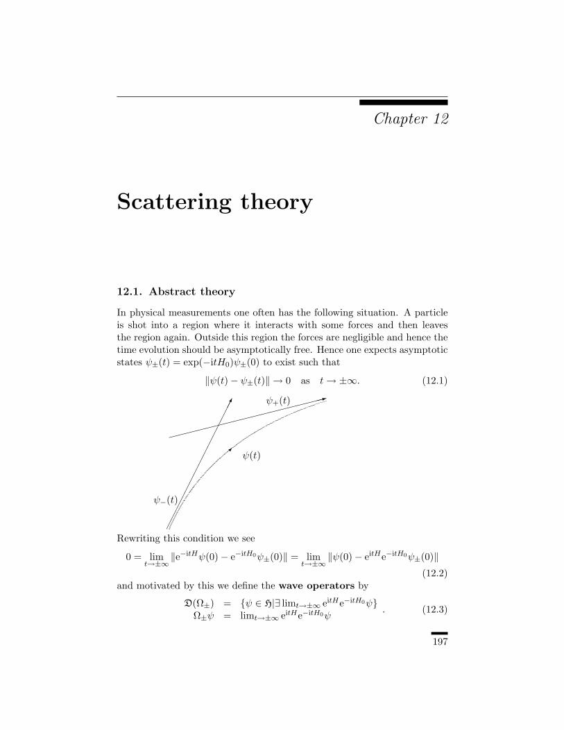
Chapter 12
Scattering theory
12.1. Abstract theory
In physical measurements one often has the following situation. A particleis shot into a region where it interacts with some forces and then leavesthe region again. Outside this region the forces are negligible and hence thetime evolution should be asymptotically free. Hence one expects asymptoticstates ψ±(t) = exp(−itH0)ψ±(0) to exist such that
‖ψ(t)− ψ±(t)‖ → 0 as t→ ±∞. (12.1)
ψ(t)
ψ−(t)
ψ+(t)
:
Rewriting this condition we see
0 = limt→±∞
‖e−itHψ(0)− e−itH0ψ±(0)‖ = limt→±∞
‖ψ(0)− eitHe−itH0ψ±(0)‖(12.2)
and motivated by this we define the wave operators by
D(Ω±) = ψ ∈ H|∃ limt→±∞ eitHe−itH0ψΩ±ψ = limt→±∞ eitHe−itH0ψ
. (12.3)
197
198 12. Scattering theory
The set D(Ω±) is the set of all incoming/outgoing asymptotic states ψ± andRan(Ω±) is the set of all states which have an incoming/outgoing asymptoticstate. If a state ψ has both, that is, ψ ∈ Ran(Ω+) ∩ Ran(Ω−), it is called ascattering state.
By construction we have
‖Ω±ψ‖ = limt→±∞
‖eitHe−itH0ψ‖ = limt→±∞
‖ψ‖ = ‖ψ‖ (12.4)
and it is not hard to see that D(Ω±) is closed. Moreover, interchanging theroles of H0 and H amounts to replacing Ω± by Ω−1
± and hence Ran(Ω±) isalso closed. In summary,
Lemma 12.1. The sets D(Ω±) and Ran(Ω±) are closed and Ω± : D(Ω±) →Ran(Ω±) is unitary.
Next, observe that
limt→±∞
eitHe−itH0(e−isH0ψ) = limt→±∞
e−isH(ei(t+s)He−i(t+s)H0ψ) (12.5)
and henceΩ±e−itH0ψ = e−itHΩ±ψ, ψ ∈ D(Ω±). (12.6)
In addition, D(Ω±) is invariant under exp(−itH0) and Ran(Ω±) is invariantunder exp(−itH). Moreover, if ψ ∈ D(Ω±)⊥ then
〈ϕ, exp(−itH0)ψ〉 = 〈exp(itH0)ϕ,ψ〉 = 0, ϕ ∈ D(Ω±). (12.7)
Hence D(Ω±)⊥ is invariant under exp(−itH0) and Ran(Ω±)⊥ is invariantunder exp(−itH). Consequently, D(Ω±) reduces exp(−itH0) and Ran(Ω±)reduces exp(−itH). Moreover, differentiating (12.6) with respect to t weobtain from Theorem 5.1 the intertwining property of the wave operators.
Theorem 12.2. The subspaces D(Ω±) respectively Ran(Ω±) reduce H0 re-spectively H and the operators restricted to these subspaces are unitarilyequivalent
Ω±H0ψ = HΩ±ψ, ψ ∈ D(Ω±) ∩D(H0). (12.8)
It is interesting to know the correspondence between incoming and out-going states. Hence we define the scattering operator
S = Ω−1+ Ω−, D(S) = ψ ∈ D(Ω−)|Ω−ψ ∈ Ran(Ω+). (12.9)
Note that we have D(S) = D(Ω−) if and only if Ran(Ω−) ⊆ Ran(Ω+) andRan(S) = D(Ω+) if and only if Ran(Ω+) ⊆ Ran(Ω−). Moreover, S is unitaryfrom D(S) onto Ran(S) and we have
H0Sψ = SH0ψ, D(H0) ∩D(S). (12.10)
However, note that this whole theory is meaningless until we can showthat D(Ω±) are nontrivial. We first show a criterion due to Cook.
12.1. Abstract theory 199
Lemma 12.3 (Cook). Suppose D(H) ⊆ D(H0). If∫ ∞
0‖(H −H0) exp(∓itH0)ψ‖dt <∞, ψ ∈ D(H0), (12.11)
then ψ ∈ D(Ω±), respectively. Moreover, we even have
‖(Ω± − I)ψ‖ ≤∫ ∞
0‖(H −H0) exp(∓itH0)ψ‖dt (12.12)
in this case.
Proof. The result follows from
eitHe−itH0ψ = ψ + i∫ t
0exp(isH)(H −H0) exp(−isH0)ψds (12.13)
which holds for ψ ∈ D(H0).
As a simple consequence we obtain the following result for Schrodingeroperators in R3
Theorem 12.4. Suppose H0 is the free Schrodinger operator and H =H0 + V with V ∈ L2(R3), then the wave operators exist and D(Ω±) = H.
Proof. Since we want to use Cook’s lemma, we need to estimate
‖V ψ(s)‖2 =∫
R3
|V (x)ψ(s, x)|2dx, ψ(s) = exp(isH0)ψ, (12.14)
for given ψ ∈ D(H0). Invoking (7.34) we get
‖V ψ(s)‖ ≤ ‖ψ(s)‖∞‖V ‖ ≤1
(4πs)3/2‖ψ‖1‖V ‖, s > 0, (12.15)
at least for ψ ∈ L1(R3). Moreover, this implies∫ ∞
1‖V ψ(s)‖ds ≤ 1
4π3/2‖ψ‖1‖V ‖ (12.16)
and thus any such ψ is in D(Ω+). Since such functions are dense, we obtainD(Ω+) = H. Similarly for Ω−.
By the intertwining property ψ is an eigenfunction of H0 if and onlyif it is an eigenfunction of H. Hence for ψ ∈ Hpp(H0) it is easy to checkwhether it is in D(Ω±) or not and only the continuous subspace is of interest.We will say that the wave operators exist if all elements of Hac(H0) areasymptotic states, that is,
Hac(H0) ⊆ D(Ω±) (12.17)
and that they are complete if, in addition, all elements of Hac(H) arescattering states, that is,
Hac(H) ⊆ Ran(Ω±). (12.18)
200 12. Scattering theory
If we even haveHc(H) ⊆ Ran(Ω±), (12.19)
they are called asymptotically complete. We will be mainly interested inthe case where H0 is the free Schrodinger operator and hence Hac(H0) = H.In this later case the wave operators exist if D(Ω±) = H, they are complete ifHac(H) = Ran(Ω±), and asymptotically complete if Hc(H) = Ran(Ω±). Inparticular asymptotic completeness implies Hsc(H) = ∅ since H restrictedto Ran(Ω±) is unitarily equivalent to H0.
12.2. Incoming and outgoing states
In the remaining sections we want to apply this theory to Schrodinger op-erators. Our first goal is to give a precise meaning to some terms in theintuitive picture of scattering theory introduced in the previous section.
This physical picture suggests that we should be able to decomposeψ ∈ H into an incoming and an outgoing part. But how should incom-ing respectively outgoing be defined for ψ ∈ H? Well incoming (outgoing)means that the expectation of x2 should decrease (increase). Set x(t)2 =exp(iH0t)x2 exp(−iH0t), then, abbreviating ψ(t) = e−itH0ψ,
d
dtEψ(x(t)2) = 〈ψ(t), i[H0, x
2]ψ(t)〉 = 4〈ψ(t), Dψ(t)〉, ψ ∈ S(Rn),
(12.20)where D is the dilation operator introduced in (10.11). Hence it is naturalto consider ψ ∈ Ran(P±),
P± = PD((0,±∞)), (12.21)
as outgoing respectively incoming states. If we project a state in Ran(P±)to energies in the interval (a2, b2), we expect that it cannot be found in aball of radius proportional to a|t| as t → ±∞ (a is the minimal velocity ofthe particle, since we have assumed the mass to be two). In fact, we willshow below that the tail decays faster then any inverse power of |t|.
We first collect some properties of D which will be needed later on. Note
FD = −DF (12.22)
and hence Ff(D) = f(−D)F . To say more we will look for a transformationwhich maps D to a multiplication operator.
Since the dilation group acts on |x| only, it seems reasonable to switchto polar coordinates x = rω, (t, ω) ∈ R+ × Sn−1. Since U(s) essentiallytransforms r into r exp(s) we will replace r by ρ = ln(r). In these coordinateswe have
U(s)ψ(eρω) = e−ns/2ψ(e(ρ−s)ω) (12.23)
12.2. Incoming and outgoing states 201
and hence U(s) corresponds to a shift of ρ (the constant in front is absorbedby the volume element). Thus D corresponds to differentiation with respectto this coordinate and all we have to do to make it a multiplication operatoris to take the Fourier transform with respect to ρ.
This leads us to the Mellin transform
M : L2(Rn) → L2(R× Sn−1)
ψ(rω) → (Mψ)(λ, ω) =1√2π
∫ ∞
0r−iλψ(rω)r
n2−1dr
. (12.24)
By construction, M is unitary, that is,∫R
∫Sn−1
|(Mψ)(λ, ω)|2dλdn−1ω =∫
R+
∫Sn−1
|ψ(rω)|2rn−1drdn−1ω,
(12.25)where dn−1ω is the normalized surface measure on Sn−1. Moreover,
M−1U(s)M = e−isλ (12.26)
and henceM−1DM = λ. (12.27)
From this it is straightforward to show that
σ(D) = σac(D) = R, σsc(D) = σpp(D) = ∅ (12.28)
and that S(Rn) is a core for D. In particular we have P+ + P− = I.Using the Mellin transform we can now prove Perry’s estimate [11].
Lemma 12.5. Suppose f ∈ C∞c (R) with supp(f) ⊂ (a2, b2) for some a, b >0. For any R ∈ R, N ∈ N there is a constant C such that
‖χx| |x|<2a|t|e−itH0f(H0)PD((±R,±∞))‖ ≤ C
(1 + |t|)N, ±t ≥ 0, (12.29)
respectively.
Proof. We prove only the + case, the remaining one being similar. Considerψ ∈ S(Rn). Introducing
ψ(t, x) = e−itH0f(H0)PD((R,∞))ψ(x) = 〈Kt,x,FPD((R,∞))ψ〉= 〈Kt,x, PD((−∞,−R))ψ〉, (12.30)
where
Kt,x(p) =1
(2π)n/2ei(tp2−px)f(p2)∗, (12.31)
we see that it suffices to show
‖PD((−∞,−R))Kt,x‖2 ≤ const
(1 + |t|)2N, for |x| < 2a|t|, t > 0. (12.32)
202 12. Scattering theory
Now we invoke the Mellin transform to estimate this norm
‖PD((−∞,−R))Kt,x‖2 =∫ R
−∞
∫Sn−1
|(MKt,x)(λ, ω)|2dλdn−1ω. (12.33)
Since(MKt,x)(λ, ω) =
1(2π)(n+1)/2
∫ ∞
0f(r)eiα(r)dr (12.34)
with f(r) = f(r2)∗rn/2−1 ∈ C∞c ((a2, b2)), α(r) = tr2 + rωx − λ ln(r). Esti-mating the derivative of α we see
α′(r) = 2tr + ωx− λ/r > 0, r ∈ (a, b), (12.35)
for λ ≤ −R and t > R(2εa)−1, where ε is the distance of a to the supportof f . Hence we can find a constant such that
1|α′(r)|
≤ const
1 + |λ|+ |t|, r ∈ (a, b), (12.36)
and λ, t as above. Using this we can estimate the integral in (12.34)∣∣∣∣∫ ∞
0f(r)
1α′(r)
d
dreiα(r)dr
∣∣∣∣ ≤ const
1 + |λ|+ |t|
∣∣∣∣∫ ∞
0f ′(r)eiα(r)dr
∣∣∣∣ , (12.37)
(the last step uses integration by parts) for λ, t as above. By increasing theconstant we can even assume that it holds for t ≥ 0 and λ ≤ −R. Moreover,by iterating the last estimate we see
|(MKt,x)(λ, ω)| ≤ const
(1 + |λ|+ |t|)N(12.38)
for any N ∈ N and t ≥ 0 and λ ≤ −R. This finishes the proof.
Corollary 12.6. Suppose that f ∈ C∞c ((0,∞)) and R ∈ R. Then theoperator PD((±R,±∞))f(H0) exp(−itH0) converges strongly to 0 as t →∓∞.
Proof. Abbreviating PD = PD((±R,±∞)) and χ = χx| |x|<2a|t| we have
‖PDf(H0)e−itH0ψ‖ ≤ ‖χeitH0f(H0)∗PD‖ ‖ψ‖+‖f(H0)‖‖(I−χ)ψ‖. (12.39)
since ‖A‖ = ‖A∗‖. Taking t→ ∓∞ the first term goes to zero by our lemmaand the second goes to zero since χψ → ψ.
12.3. Schrodinger operators with short rangepotentials
By the RAGE theorem we know that for ψ ∈ Hc, ψ(t) will eventually leaveevery compact ball (at least on the average). Hence we expect that thetime evolution will asymptotically look like the free one for ψ ∈ Hc if thepotential decays sufficiently fast. In other words, we expect such potentialsto be asymptotically complete.
12.3. Schrodinger operators with short range potentials 203
Suppose V is relatively bounded with bound less than one. Introduce
h1(r) = ‖V RH0(z)χr‖, h2(r) = ‖χrV RH0(z)‖, r ≥ 0, (12.40)
whereχr = χx| |x|≥r. (12.41)
The potential V will be called short range if these quantities are integrable.We first note that it suffices to check this for h1 or h2 and for one z ∈ ρ(H0).
Lemma 12.7. The function h1 is integrable if and only if h2 is. Moreover,hj integrable for one z0 ∈ ρ(H0) implies hj integrable for all z ∈ ρ(H0).
Proof. Pick φ ∈ C∞c (Rn, [0, 1]) such that φ(x) = 0 for 0 ≤ |x| ≤ 1/2 andφ(x) = 0 for 1 ≤ |x|. Then it is not hard to see that hj is integrable if andonly if hj is integrable, where
h1(r) = ‖V RH0(z)φr‖, h2(r) = ‖φrV RH0(z)‖, r ≥ 1, (12.42)
and φr(x) = φ(x/r). Using
[RH0(z), φr] = −RH0(z)[H0(z), φr]RH0(z)
= RH0(z)(∆φr + (∂φr)∂)RH0(z) (12.43)
and ∆φr = φr/2∆φr, ‖∆φr‖∞ ≤ ‖∆φ‖∞/r2 respectively (∂φr) = φr/2(∂φr),‖∂φr‖∞ ≤ ‖∂φ‖∞/r2 we see
|h1(r)− h2(r)| ≤c
rh1(r/2), r ≥ 1. (12.44)
Hence h2 is integrable if h1 is. Conversely,
h1(r) ≤ h2(r) +c
rh1(r/2) ≤ h2(r) +
c
rh2(r/2) +
2cr2h1(r/4) (12.45)
shows that h2 is integrable if h1 is.Invoking the first resolvent formula
‖φrV RH0(z)‖ ≤ ‖φrV RH0(z0)‖‖I− (z − z0)RH0(z)‖ (12.46)
finishes the proof.
As a first consequence note
Lemma 12.8. If V is short range, then RH(z)−RH0(z) is compact.
Proof. The operator RH(z)V (I−χr)RH0(z) is compact since (I−χr)RH0(z)is by Lemma 7.10 and RH(z)V is bounded by Lemma 6.22. Moreover, byour short range condition it converges in norm to
RH(z)V RH0(z) = RH(z)−RH0(z) (12.47)
as r →∞ (at least for some subsequence).
204 12. Scattering theory
In particular, by Weyl’s theorem we have σess(H) = [0,∞). Moreover,V short range implies that H and H0 look alike far outside.
Lemma 12.9. Suppose RH(z)−RH0(z) is compact, then so is f(H)−f(H0)for any f ∈ C∞(R) and
limr→∞
‖(f(H)− f(H0))χr‖ = 0. (12.48)
Proof. The first part is Lemma 6.20 and the second part follows from part(ii) of Lemma 6.8 since χr converges strongly to 0.
However, this is clearly not enough to prove asymptotic completenessand we need a more careful analysis. The main ideas are due to Enß [4].
We begin by showing that the wave operators exist. By Cook’s criterion(Lemma 12.3) we need to show that
‖V exp(∓itH0)ψ‖ ≤ ‖V RH0(−1)‖‖(I− χ2a|t|) exp(∓itH0)(H0 + I)ψ‖+ ‖V RH0(−1)χ2a|t|‖‖(H0 + I)ψ‖ (12.49)
is integrable for a dense set of vectors ψ. The second term is integrable by ourshort range assumption. The same is true by Perry’s estimate (Lemma 12.5)for the first term if we choose ψ = f(H0)PD((±R,±∞))ϕ. Since vectors ofthis form are dense, we see that the wave operators exist,
D(Ω±) = H. (12.50)
Since H restricted to Ran(Ω∗±) is unitarily equivalent to H0, we obtain
[0,∞) = σac(H0) ⊆ σac(H). And by σac(H) ⊆ σess(H) = [0,∞) we evenhave σac(H) = [0,∞).
To prove asymptotic completeness of the wave operators we will needthat (Ω± − I)f(H0)P± are compact.
Lemma 12.10. Let f ∈ C∞c ((0,∞)) and suppose ψn converges weakly to 0.Then
limn→∞
‖(Ω± − I)f(H0)P±ψn‖ = 0, (12.51)
that is, (Ω± − I)f(H0)P± is compact.
Proof. By (12.13) we see
‖RH(z)(Ω± − I)f(H0)P±ψn‖ ≤∫ ∞
0‖RH(z)V exp(−isH0)f(H0)P±ψn‖dt.
(12.52)Since RH(z)V RH0 is compact we see that the integrand
RH(z)V exp(−isH0)f(H0)P±ψn =
RH(z)V RH0 exp(−isH0)(H0 + 1)f(H0)P±ψn (12.53)
12.3. Schrodinger operators with short range potentials 205
converges pointwise to 0. Moreover, arguing as in (12.49) the integrandis bounded by an L1 function depending only on ‖ψn‖. Thus RH(z)(Ω± −I)f(H0)P± is compact by the dominated convergence theorem. Furthermore,using the intertwining property we see that
(Ω± − I)f(H0)P± = RH(z)(Ω± − I)f(H0)P±− (RH(z)−RH0(z))f(H0)P± (12.54)
is compact by Lemma 6.20, where f(λ) = (λ+ 1)f(λ).
Now we have gathered enough information to tackle the problem ofasymptotic completeness.
We first show that the singular continuous spectrum is absent. Thisis not really necessary, but avoids the use of Cesaro means in our mainargument.
Abbreviate P = P scH PH((a, b)), 0 < a < b. Since H restricted toRan(Ω±) is unitarily equivalent to H0 (which has purely absolutely continu-ous spectrum), the singular part must live on Ran(Ω±)⊥, that is, P scH Ω± = 0.Thus Pf(H0) = P (I−Ω+)f(H0)P+ +P (I−Ω−)f(H0)P− is compact. Sincef(H) − f(H0) is compact, it follows that Pf(H) is also compact. Choos-ing f such that f(λ) = 1 for λ ∈ [a, b] we see that P = Pf(H) is com-pact and hence finite dimensional. In particular σsc(H) ∩ (a, b) is a fi-nite set. But a continuous measure cannot be supported on a finite set,showing σsc(H) ∩ (a, b) = ∅. Since 0 < a < b are arbitrary we evenhave σsc(H) ∩ (0,∞) = ∅ and by σsc(H) ⊆ σess(H) = [0,∞) we obtainσsc(H) = ∅.
Observe that replacing P scH by P ppH the same argument shows that allnonzero eigenvalues are finite dimensional and cannot accumulate in (0,∞).
In summary we have shown
Theorem 12.11. Suppose V is short range. Then
σac(H) = σess(H) = [0,∞), σsc(H) = ∅. (12.55)
All nonzero eigenvalues have finite multiplicity and cannot accumulate in(0,∞).
Now we come to the anticipated asymptotic completeness result of Enß.Choose
ψ ∈ Hc(H) = Hac(H) such that ψ = f(H)ψ (12.56)
for some f ∈ C∞c ((0,∞). By the RAGE theorem the sequence ψ(t) convergesweakly to zero as t→ ±∞. Abbreviate ψ(t) = exp(−itH)ψ. Introduce
ϕ±(t) = f(H0)P±ψ(t). (12.57)
206 12. Scattering theory
which satisfylim
t→±∞‖ψ(t)− ϕ+(t)− ϕ−(t)‖ = 0. (12.58)
Indeed this follows from
ψ(t) = ϕ+(t) + ϕ−(t) + (f(H)− f(H0))ψ(t) (12.59)
and Lemma 6.20. Moreover, we even have
limt→±∞
‖(Ω± − I)ϕ±(t)‖ = 0 (12.60)
by Lemma 12.10. Now suppose ψ ∈ Ran(Ω±)⊥, then
‖ψ‖2 = limt→±∞
〈ψ(t), ψ(t)〉
= limt→±∞
〈ψ(t), ϕ+(t) + ϕ−(t)〉
= limt→±∞
〈ψ(t),Ω+ϕ+(t) + Ω−ϕ−(t)〉. (12.61)
By Theorem 12.2, Ran(Ω±)⊥ is invariant underH and hence ψ(t) ∈ Ran(Ω±)⊥
implying
‖ψ‖2 = limt→±∞
〈ψ(t),Ω∓ϕ∓(t)〉 (12.62)
= limt→±∞
〈P∓f(H0)∗Ω∗∓ψ(t), ψ(t)〉.
Invoking the intertwining property we see
‖ψ‖2 = limt→±∞
〈P∓f(H0)∗e−itH0Ω∗∓ψ,ψ(t)〉 = 0 (12.63)
by Corollary 12.6. Hence Ran(Ω±) = Hac(H) = Hc(H) and we thus haveshown
Theorem 12.12 (Enß). Suppose V is short range, then the wave operatorsare asymptotically complete.
For further results and references see for example [3].

Part 3
Appendix

Appendix A
Almost everythingabout Lebesgueintegration
In this appendix I give a brief introduction to measure theory. Good refer-ences are [2] or [18].
A.1. Borel measures in a nut shell
The first step in defining the Lebesgue integral is extending the notion ofsize from intervals to arbitrary sets. Unfortunately, this turns out to be toomuch, since a classical paradox by Banach and Tarski shows that one canbreak the unit ball in R3 into a finite number of (wild – choosing the piecesuses the Axiom of Choice and cannot be done with a jigsaw;-) pieces, rotateand translate them, and reassemble them to get two copies of the unit ball(compare Problem A.1). Hence any reasonable notion of size (i.e., one whichis translation and rotation invariant) cannot be defined for all sets!
A collection of subsets A of a given set X such that
• X ∈ A,
• A is closed under finite unions,
• A is closed under complements.
is called an algebra. Note that ∅ ∈ A and that, by de Morgan, A is alsoclosed under finite intersections. If an algebra is closed under countableunions (and hence also countable intersections), it is called a σ-algebra.
209
210 A. Almost everything about Lebesgue integration
Moreover, the intersection of any family of (σ-)algebras Aα is againa (σ-)algebra and for any collection S of subsets there is a unique smallest(σ-)algebra Σ(S) containing S (namely the intersection of all (σ-)algebracontaining S). It is called the (σ-)algebra generated by S.
If X is a topological space, the Borel σ-algebra of X is defined to bethe σ-algebra generated by all open (respectively all closed) sets. Sets in theBorel σ-algebra are called Borel sets.Example. In the case X = Rn the Borel σ-algebra will be denoted by Bn
and we will abbreviate B = B1.
Now let us turn to the definition of a measure: A setX together with a σ-algebra Σ is called a measure space. A measure µ is a map µ : Σ → [0,∞]on a σ-algebra Σ such that
• µ(∅) = 0,
• µ(⋃∞j=1Aj) =
∑∞j=1 µ(Aj) if Aj∩Ak = ∅ for all j, k (σ-additivity).
It is called σ-finite if there is a countable cover Xj∞j=1 of X with µ(Xj) <∞ for all j. (Note that it is no restriction to assume Xj X.) It is calledfinite if µ(X) <∞. The sets in Σ are called measurable sets.
If we replace the σ-algebra by an algebra A, then µ is called a premea-sure. In this case σ-additivity clearly only needs to hold for disjoint setsAn for which
⋃nAn ∈ A.
We will write An A if An ⊆ An+1 (note A =⋃nAn) and An A if
An+1 ⊆ An (note A =⋂nAn).
Theorem A.1. Any measure µ satisfies the following properties:
(i) A ⊆ B implies µ(A) ≤ µ(B) (monotonicity).
(ii) µ(An) → µ(A) if An A (continuity from below).
(iii) µ(An) → µ(A) if An A and µ(A1) <∞ (continuity from above).
Proof. The first claim is obvious. The second follows using An = An\An−1
and σ-additivity. The third follows from the second using An = A1\An andµ(An) = µ(A1)− µ(An).
Example. Let A ∈ P(M) and set µ(A) to be the number of elements of A(respectively ∞ if A is infinite). This is the so called counting measure.
Note that if X = N and An = j ∈ N|j ≥ n, then µ(An) = ∞, butµ(⋂nAn) = µ(∅) = 0 which shows that the requirement µ(A1) < ∞ in the
last claim of Theorem A.1 is not superfluous.
A.1. Borel measures in a nut shell 211
A measure on the Borel σ-algebra is called a Borel measure if µ(C) <∞ for any compact set C. A Borel measures is called outer regular if
µ(A) = infA⊆O,O open
µ(O) (A.1)
and inner regular if
µ(A) = supC⊆A,C compact
µ(C). (A.2)
It is called regular if it is both outer and inner regular.But how can we obtain some more interesting Borel measures? We will
restrict ourselves to the case of X = R for simplicity. Then the strategyis as follows: Start with the algebra of finite unions of disjoint intervalsand define µ for those sets (as the sum over the intervals). This yields apremeasure. Extend this to an outer measure for all subsets of R. Showthat the restriction to the Borel sets is a measure.
Let us first show how we should define µ for intervals: To every Borelmeasure on B we can assign its distribution function
µ(x) =
−µ((x, 0]), x < 00, x = 0µ((0, x]), x > 0
(A.3)
which is right continuous and non-decreasing. Conversely, given a rightcontinuous non-decreasing function µ : R → R we can set
µ(A) =
µ(b)− µ(a), A = (a, b]µ(b)− µ(a−), A = [a, b]µ(b−)− µ(a), A = (a, b)µ(b−)− µ(a−), A = [a, b)
, (A.4)
where µ(a−) = limε↓0 µ(a−ε). In particular, this gives a premeasure on thealgebra of finite unions of intervals which can be extended to a measure:
Theorem A.2. For every right continuous non-decreasing function µ : R →R there exists a unique regular Borel measure µ which extends (A.4). Twodifferent functions generate the same measure if and only if they differ by aconstant.
Since the proof of this theorem is rather involved, we defer it to the nextsection and look at some examples first.Example. Suppose Θ(x) = 0 for x < 0 and Θ(x) = 1 for x ≥ 0. Then weobtain the so-called Dirac measure at 0, which is given by Θ(A) = 1 if0 ∈ A and Θ(A) = 0 if 0 6∈ A.
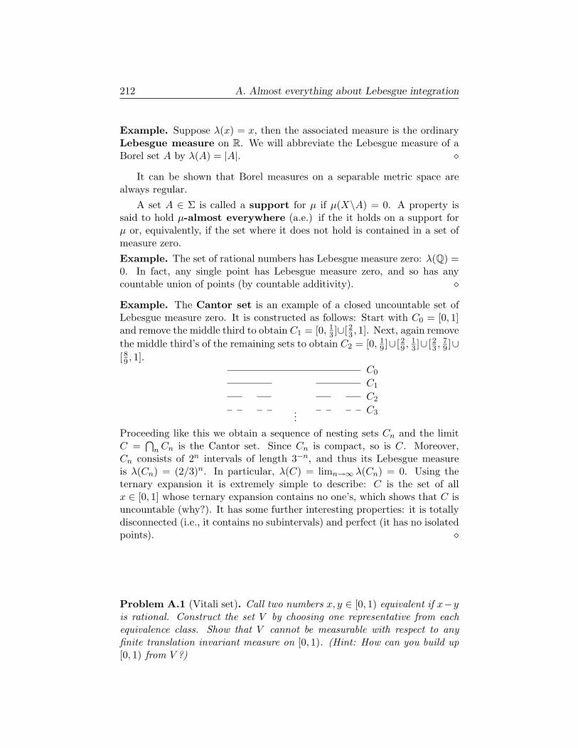
212 A. Almost everything about Lebesgue integration
Example. Suppose λ(x) = x, then the associated measure is the ordinaryLebesgue measure on R. We will abbreviate the Lebesgue measure of aBorel set A by λ(A) = |A|.
It can be shown that Borel measures on a separable metric space arealways regular.
A set A ∈ Σ is called a support for µ if µ(X\A) = 0. A property issaid to hold µ-almost everywhere (a.e.) if the it holds on a support forµ or, equivalently, if the set where it does not hold is contained in a set ofmeasure zero.Example. The set of rational numbers has Lebesgue measure zero: λ(Q) =0. In fact, any single point has Lebesgue measure zero, and so has anycountable union of points (by countable additivity).
Example. The Cantor set is an example of a closed uncountable set ofLebesgue measure zero. It is constructed as follows: Start with C0 = [0, 1]and remove the middle third to obtain C1 = [0, 1
3 ]∪[23 , 1]. Next, again removethe middle third’s of the remaining sets to obtain C2 = [0, 1
9 ]∪ [29 ,13 ]∪ [23 ,
79 ]∪
[89 , 1].C0
C1
C2
C3...Proceeding like this we obtain a sequence of nesting sets Cn and the limitC =
⋂nCn is the Cantor set. Since Cn is compact, so is C. Moreover,
Cn consists of 2n intervals of length 3−n, and thus its Lebesgue measureis λ(Cn) = (2/3)n. In particular, λ(C) = limn→∞ λ(Cn) = 0. Using theternary expansion it is extremely simple to describe: C is the set of allx ∈ [0, 1] whose ternary expansion contains no one’s, which shows that C isuncountable (why?). It has some further interesting properties: it is totallydisconnected (i.e., it contains no subintervals) and perfect (it has no isolatedpoints).
Problem A.1 (Vitali set). Call two numbers x, y ∈ [0, 1) equivalent if x−yis rational. Construct the set V by choosing one representative from eachequivalence class. Show that V cannot be measurable with respect to anyfinite translation invariant measure on [0, 1). (Hint: How can you build up[0, 1) from V ?)
A.2. Extending a premasure to a measure 213
A.2. Extending a premasure to a measure
The purpose of this section is to prove Theorem A.2. It is rather technical andshould be skipped on first reading.
In order to prove Theorem A.2 we need to show how a premeasure canbe extended to a measure. As a prerequisite we first establish that it sufficesto check increasing (or decreasing) sequences of sets when checking wethera given algebra is in fact a σ-algebra:
A collections of sets M is called a monotone class if An A impliesA ∈M whenever An ∈M and An A implies A ∈M whenever An ∈M.Every σ-algebra is a monotone class and the intersection of monotone classesis a monotone class. Hence every collection of sets S generates a smallestmonotone class M(S).
Theorem A.3. Let A be an algebra. Then M(A) = Σ(A).
Proof. We first show that M = M(A) is an algebra.Put M(A) = B ∈ M|A ∪ B ∈ M. If Bn is an increasing sequence
of sets in M(A) then A ∪ Bn is an increasing sequence in M and hence⋃n(A ∪Bn) ∈M. Now
A ∪(⋃
n
Bn
)=⋃n
(A ∪Bn) (A.5)
shows that M(A) is closed under increasing sequences. Similarly, M(A) isclosed under decreasing sequences and hence it is a monotone class. Butdoes it contain any elements? Well if A ∈ A we have A ⊆ M(A) implyingM(A) = M. Hence A ∪B ∈ M if at least one of the sets is in A. But thisshows A ⊆ M(A) and hence M(A) = M for any A ∈ M. So M is closedunder finite unions.
To show that we are closed under complements consider M = A ∈M|X\A ∈ M. If An is an increasing sequence then X\An is a decreasingsequence and X\
⋃nAn =
⋂nX\An ∈M if An ∈M . Similarly for decreas-
ing sequences. Hence M is a monotone class and must be equal to M sinceit contains A.
So we know that M is an algebra. To show that it is an σ-algebra letAn be given and put An =
⋃k≤nAn. Then An is increasing and
⋃n An =⋃
nAn ∈ A.
The typical use of this theorem is as follows: First verify some propertyfor sets in an algebra A. In order to show that it holds for any set in Σ(A),it suffices to show that the sets for which it holds is closed under countableincreasing and decreasing sequences (i.e., is a monotone class).
Now we start by proving that (A.4) indeed gives rise to a premeasure.
214 A. Almost everything about Lebesgue integration
Lemma A.4. µ as defined in (A.4) gives rise to a unique σ-finite regularpremeasure on the algebra A of finite unions of disjoint intervals.
Proof. First of all, (A.4) can be extended to finite unions of disjoint inter-vals by summing over all intervals. It is straightforward to verify that µ iswell defined (one set can be represented by different unions of intervals) andby construction additive.
To show regularity, we can assume any such union to consist of openintervals and points only. To show outer regularity replace each point xby a small open interval (x+ε, x−ε) and use that µ(x) = limε↓ µ(x+ε)−µ(x−ε). Similarly, to show inner regularity, replace each open interval (a, b)by a compact one [an, bn] ⊆ (a, b) and use µ((a, b)) = limn→∞ µ(bn)− µ(an)if an ↓ a and bn ↑ b.
It remains to verify σ-additivity. We need to show
µ(⋃k
Ik) =∑k
µ(Ik) (A.6)
whenever In ∈ A and I =⋃k Ik ∈ A. Since each In is a finite union of in-
tervals, we can as well assume each In is just one interval (just split In intoits subintervals and note that the sum does not change by additivity). Sim-ilarly, we can assume that I is just one interval (just treat each subintervalseparately).
By additivity µ is monotone and hence
n∑k=1
µ(Ik) = µ(n⋃k=1
Ik) ≤ µ(I) (A.7)
which shows∞∑k=1
µ(Ik) ≤ µ(I). (A.8)
To get the converse inequality we need to work harder.By outer regularity we can cover each Ik by open interval Jk such that
µ(Jk) ≤ µ(Ik) + ε2k . Suppose I is compact first. Then finitely many of the
Jk, say the first n, cover I and we have
µ(I) ≤ µ(n⋃k=1
Jk) ≤n∑k=1
µ(Jk) ≤∞∑k=1
µ(Ik) + ε. (A.9)
Since ε > 0 is arbitrary, this shows σ-additivity for compact intervals. Byadditivity we can always add/subtract the end points of I and hence σ-additivity holds for any bounded interval. If I is unbounded, say I = [a,∞),
A.2. Extending a premasure to a measure 215
then given x > 0 we can find an n such that Jn cover at least [0, x] and hencen∑k=1
µ(Ik) ≥n∑k=1
µ(Jk)− ε ≥ µ([a, x])− ε. (A.10)
Since x > a and ε > 0 are arbitrary we are done.
This premeasure determines the corresponding measure µ uniquely (ifthere is one at all):
Theorem A.5 (Uniqueness of measures). Let µ be a σ-finite premeasureon an algebra A. Then there is at most one extension to Σ(A).
Proof. We first assume that µ(X) <∞. Suppose there is another extensionµ and consider the set
S = A ∈ Σ(A)|µ(A) = µ(A). (A.11)
I claim S is a monotone class and hence S = Σ(A) since A ⊆ S by assump-tion (Theorem A.3).
Let An A. If An ∈ S we have µ(An) = µ(An) and taking limits(Theorem A.1 (ii)) we conclude µ(A) = µ(A). Next let An A and takeagain limits. This finishes the finite case. To extend our result to the σ-finitecase let Xj X be an increasing sequence such that µ(Xj) < ∞. By thefinite case µ(A ∩Xj) = µ(A ∩Xj) (just restrict µ, µ to Xj). Hence
µ(A) = limj→∞
µ(A ∩Xj) = limj→∞
µ(A ∩Xj) = µ(A) (A.12)
and we are done.
Note that if our premeasure is regular, so will be the extension:
Lemma A.6. Suppose µ is a σ-finite premeasure on some algebra A gen-erating the Borel sets B. Then outer (inner) regularity holds for all Borelsets if it holds for all sets in A.
Proof. We first assume that µ(X) <∞. Set
µ(A) = infA⊆O,O open
µ(O) ≥ µ(A) (A.13)
and let M = A ∈ B|µ(A) = µ(A). Since by assumption M containssome algebra generating B it suffices to proof that M is a monotone class.
Let An ∈M be a monotone sequence and let On ⊇ An be open sets suchthat µ(On) ≤ µ(An) + 1
n . Then
µ(An) ≤ µ(An) ≤ µ(On) ≤ µ(An) +1n. (A.14)
Now if An A just take limits and use continuity from below of µ. Similarlyif An A.
216 A. Almost everything about Lebesgue integration
Now let µ be arbitrary. Given A we can split it into disjoint sets Ajsuch that Aj ⊆ Xj (A1 = A ∩ X1, A2 = (A\A1) ∩ X2, etc.). Let Xj be acover with µ(Xj) <∞. By regularity, we can assume Xj open. Thus thereare open (in X) sets Oj covering Aj such that µ(Oj) ≤ µ(Aj) + ε
2j . ThenO =
⋃j Oj is open, covers A, and satisfies
µ(A) ≤ µ(O) ≤∑j
µ(Oj) ≤ µ(A) + ε. (A.15)
This settles outer regularity.Next let us turn to inner regularity. If µ(X) <∞ one can show as before
that M = A ∈ B|µ(A) = µ(A), where
µ(A) = supC⊆A,C compact
µ(C) ≤ µ(A) (A.16)
is a monotone class. This settles the finite case.For the σ-finite case split again A as before. Since Xj has finite measure,
there are compact subsets Kj of Aj such that µ(Aj) ≤ µ(Kj) + ε2j . Now
we need to distinguish two cases: If µ(A) = ∞, the sum∑
j µ(Aj) willdiverge and so will
∑j µ(Kj). Hence Kn =
⋃nj=1 ⊆ A is compact with
µ(Kn) → ∞ = µ(A). If µ(A) < ∞, the sum∑
j µ(Aj) will converge andchoosing n sufficiently large we will have
µ(Kn) ≤ µ(A) ≤ µ(Kn) + 2ε. (A.17)
This finishes the proof.
So it remains to ensure that there is an extension at all. For any pre-measure µ we define
µ∗(A) = inf ∞∑n=1
µ(An)∣∣∣A ⊆ ∞⋃
n=1
An, An ∈ A
(A.18)
where the infimum extends over all countable covers from A. Then thefunction µ∗ : P(X) → [0,∞] is an outer measure, that is, it has theproperties (Problem A.2)
• µ∗(∅) = 0,
• A1 ⊆ A2 ⇒ µ∗(A1) ≤ µ∗(A2), and
• µ∗(⋃∞n=1An) ≤
∑∞n=1 µ
∗(An) (subadditivity).
Note that µ∗(A) = µ(A) for A ∈ A (Problem A.3).
Theorem A.7 (Extensions via outer measures). Let µ∗ be an outer measure.Then the set Σ of all sets A satisfying the Caratheodory condition
µ∗(E) = µ∗(A ∩ E) + µ∗(A′ ∩ E) ∀E ⊆ X (A.19)
A.2. Extending a premasure to a measure 217
(where A′ = X\A is the complement of A) form a σ-algebra and µ∗ restrictedto this σ-algebra is a measure.
Proof. We first show that Σ is an algebra. It clearly containsX and is closedunder complements. Let A,B ∈ Σ. Applying Caratheodory’s conditiontwice finally shows
µ∗(E) = µ∗(A ∩B ∩ E) + µ∗(A′∩B ∩ E) + µ∗(A ∩B′∩ E)
+ µ∗(A′∩B′∩ E)
≥ µ∗((A ∪B) ∩ E) + µ∗((A ∪B)′∩ E), (A.20)
where we have used De Morgan and
µ∗(A∩B ∩E)+µ∗(A′∩B ∩E)+µ∗(A∩B′∩E) ≥ µ∗((A∪B)∩E) (A.21)
which follows from subadditivity and (A ∪ B) ∩ E = (A ∩ B ∩ E) ∪ (A′∩B ∩E) ∪ (A ∩B′∩E). Since the reverse inequality is just subadditivity, weconclude that Σ is an algebra.
Next, let An be a sequence of sets from Σ. Without restriction wecan assume that they are disjoint (compare the last argument in proof ofTheorem A.3). Abbreviate An =
⋃k≤nAn, A =
⋃nAn. Then for any set E
we have
µ∗(An ∩ E) = µ∗(An ∩ An ∩ E) + µ∗(A′n∩ An ∩ E)
= µ∗(An ∩ E) + µ∗(An−1 ∩ E)
= . . . =n∑k=1
µ∗(Ak ∩ E). (A.22)
Using An ∈ Σ and monotonicity of µ∗, we infer
µ∗(E) = µ∗(An ∩ E) + µ∗(A′n∩ E)
≥n∑k=1
µ∗(Ak ∩ E) + µ∗(A′∩ E). (A.23)
Letting n→∞ and using subadditivity finally gives
µ∗(E) ≥∞∑k=1
µ∗(Ak ∩ E) + µ∗(A′∩ E)
≥ µ∗(A ∩ E) + µ∗(B′∩ E) ≥ µ∗(E) (A.24)
and we infer that Σ is a σ-algebra.Finally, setting E = A in (A.24) we have
µ∗(A) =∞∑k=1
µ∗(Ak ∩A) + µ∗(A′∩A) =∞∑k=1
µ∗(Ak) (A.25)
and we are done.
218 A. Almost everything about Lebesgue integration
Remark: The constructed measure µ is complete, that is, for any mea-surable set A of measure zero, any subset of A is again measurable (Prob-lem A.4).
The only remaining question is wether there are any nontrivial sets sat-isfying the Caratheodory condition.
Lemma A.8. Let µ be a premeasure on A and let µ∗ be the associated outermeasure. Then every set in A satisfies the Caratheodory condition.
Proof. Let An ∈ A be a countable cover for E. Then for any A ∈ A wehave
∞∑n=1
µ(An) =∞∑n=1
µ(An∩A)+∞∑n=1
µ(An∩A′) ≥ µ∗(E∩A)+µ∗(E∩A′) (A.26)
since An ∩A ∈ A is a cover for E ∩A and An ∩A′ ∈ A is a cover for E ∩A′.Taking the infimum we have µ∗(E) ≥ µ∗(E ∩A)+µ∗(E ∩A′) which finishesthe proof.
Thus, as a consequence we obtain Theorem A.2.
Problem A.2. Show that µ∗ defined in (A.18) is an outer measure. (Hintfor the last property: Take a cover Bnk∞k=1 for An such that µ∗(An) =ε2n +
∑∞k=1 µ(Bnk) and note that Bnk∞n,k=1 is a cover for
⋃nAn.)
Problem A.3. Show that µ∗ defined in (A.18) extends µ. (Hint: For thecover An it is no restriction to assume An ∩Am = ∅ and An ⊆ A.)
Problem A.4. Show that the measure constructed in Theorem A.7 is com-plete.
A.3. Measurable functions
The Riemann integral works by splitting the x coordinate into small intervalsand approximating f(x) on each interval by its minimum and maximum.The problem with this approach is that the difference between maximumand minimum will only tend to zero (as the intervals get smaller) if f(x) issufficiently nice. To avoid this problem we can force the difference to go tozero by considering, instead of an interval, the set of x for which f(x) liesbetween two given numbers a < b. Now we need the size of the set of thesex, that is, the size of the preimage f−1((a, b)). For this to work, preimagesof intervals must be measurable.
A function f : X → Rn is called measurable if f−1(A) ∈ Σ for everyA ∈ Bn. A complex-valued function is called measurable if both its realand imaginary parts are. Clearly it suffices to check this condition for every

A.3. Measurable functions 219
set A in a collection of sets which generate Bn, say for all open intervals oreven for open intervals which are products of (a,∞):
Lemma A.9. A function f : X → Rn is measurable if and only if
f−1(I) ∈ Σ ∀ I =n∏j=1
(aj ,∞). (A.27)
In particular, a function f : X → Rn is measurable if and only if everycomponent is measurable.
Proof. All you have to use is f−1(Rn\A) = X\f−1(A), f−1(⋃j Aj) =⋃
j f1(Aj) and the fact that any open set is a countable union of open
intervals.
If Σ is the Borel σ-algebra, we will call a measurable function also Borelfunction. Note that, in particular,
Lemma A.10. Any continuous function is measurable and the compositionof two measurable functions is again measurable.
Moreover, sometimes it is also convenient to allow ±∞ as possible valuesfor f , that is, functions f : X → R, R = R ∪ −∞,∞. In this case A ⊆ Ris called Borel if A ∩ R is.
The set of all measurable functions forms an algebra.
Lemma A.11. Suppose f, g : X → R are measurable functions. Then thesum f + g and the product fg is measurable.
Proof. Note that addition and multiplication are continuous functions fromR2 → R and hence the claim follows from the previous lemma.
Moreover, the set of all measurable functions is closed under all impor-tant limiting operations.
Lemma A.12. Suppose fn : X → R is a sequence of measurable functions,then
infn∈N
fn, supn∈N
fn, lim infn→∞
fn, lim supn→∞
fn (A.28)
are measurable as well.
Proof. It suffices to proof that sup fn is measurable since the rest followsfrom inf fn = − sup(−fn), lim inf fn = supk infn≥k fn, and lim sup fn =infk supn≥k fn. But (sup fn)−1((a,∞)) =
⋃n f
−1n ((a,∞)) and we are done.
It follows that if f and g are measurable functions, so are min(f, g),max(f, g), |f | = max(f,−f), f± = max(±f, 0).
220 A. Almost everything about Lebesgue integration
A.4. The Lebesgue integral
Now we can define the integral for measurable functions as follows. Ameasurable function s : X → R is called simple if its range is finites(X) = αjpj=1, that is, if
s =p∑j=1
αj χAj , Aj = s−1(αj) ∈ Σ. (A.29)
Here χA is the characteristic function of A, that is, χA(x) = 1 if x ∈ Aand χA(x) = 0 else.
For a positive simple function we define its integral as∫As dµ =
n∑j=1
αj µ(Aj ∩A). (A.30)
Here we use the convention 0 · ∞ = 0.
Lemma A.13. The integral has the following properties:
(i)∫A s dµ =
∫X χA s dµ.
(ii)∫S∞
j=1 Ajs dµ =
∑∞j=1
∫Ajs dµ.
(iii)∫A α s dµ = α
∫A s dµ.
(iv)∫A(s+ t)dµ =
∫A s dµ+
∫A t dµ.
(v) A ⊆ B ⇒∫A s dµ ≤
∫B s dµ.
(vi) s ≤ t ⇒∫A s dµ ≤
∫A t dµ.
Proof. (i) is clear from the definition. (ii) follows from σ-additivity of µ.(iii) is obvious. (iv) Let s =
∑j αj χAj , t =
∑j βj χBj and abbreviate
Cjk = (Aj ∩Bk) ∩A. Then∫A(s+ t)dµ =
∑j,k
∫Cjk
(s+ t)dµ =∑j,k
(αj + βk)µ(Cjk)
=∑j,k
(∫Cjk
s dµ+∫Cjk
t dµ
)=∫As dµ+
∫At dµ(A.31)
(v) follows from monotonicity of µ. (vi) follows using t− s ≥ 0 and arguingas in (iii).
Our next task is to extend this definition to arbitrary positive functionsby ∫
Af dµ = sup
s≤f
∫As dµ, (A.32)
A.4. The Lebesgue integral 221
where the supremum is taken over all simple functions s ≤ f . Note that,except for possibly (ii) and (iv), Lemma A.13 still holds for this extension.
Theorem A.14 (monotone convergence). Let fn be a monotone non-decreas-ing sequence of positive measurable functions, fn f . Then∫
Afn dµ→
∫Af dµ. (A.33)
Proof. By property (v)∫A fn dµ is monotone and converges to some number
α. By fn ≤ f and again (v) we have
α ≤∫Af dµ. (A.34)
To show the converse let s be simple such that s ≤ f and let θ ∈ (0, 1). PutAn = x ∈ A|fn(x) ≥ θs(x) and note An X (show this). Then∫
Afn dµ ≥
∫An
fn dµ ≥ θ
∫An
s dµ. (A.35)
Letting n→∞ we see
α ≥ θ
∫As dµ. (A.36)
Since this is valid for any θ < 1, it still holds for θ = 1. Finally, since s ≤ fis arbitrary, the claim follows.
In particular ∫Af dµ = lim
n→∞
∫Asn dµ, (A.37)
for any monotone sequence sn f of simple functions. Note that there isalways such a sequence, for example,
sn(x) =n2∑k=0
k
nχf−1(Ak)(x), Ak = [
k
n,k + 1n2
), An2 = [n,∞). (A.38)
By construction sn converges uniformly if f is bounded, since sn(x) = n iff(x) = ∞ and f(x)− sn(x) < 1
n if f(x) < n+ 1.Now what about the missing items (ii) and (iv) from Lemma A.13? Since
limits can be spread over sums, the extension is linear (i.e., item (iv) holds)and (ii) also follows directly from the monotone convergence theorem. Weeven have the following result:
Lemma A.15. If f ≥ 0 is measurable, then dν = f dµ defined via
ν(A) =∫Af dµ (A.39)
222 A. Almost everything about Lebesgue integration
is a measure such that ∫g dν =
∫gf dµ. (A.40)
Proof. As already mentioned, additivity of µ is equivalent to linearity of theintegral and σ-additivity follows from the monotone convergence theorem
ν(∞⋃n=1
An) =∫
(∞∑n=1
χAn)f dµ =∞∑n=1
∫χAnf dµ =
∞∑n=1
ν(An). (A.41)
The second claim holds for simple functions and hence for all functions byconstruction of the integral.
If fn is not necessarily monotone we have at least
Theorem A.16 (Fatou’s Lemma). If fn is a sequence of nonnegative mea-surable function, then∫
Alim infn→∞
fn dµ ≤ lim infn→∞
∫Afn dµ, (A.42)
Proof. Set gn = infk≥n fk. Then gn ≤ fn implying∫Agn dµ ≤
∫Afn dµ. (A.43)
Now take the lim inf on both sides and note that by the monotone conver-gence theorem
lim infn→∞
∫Agn dµ = lim
n→∞
∫Agn dµ =
∫A
limn→∞
gn dµ =∫A
lim infn→∞
fn dµ,
(A.44)proving the claim.
If the integral is finite for both the positive and negative part f± of anarbitrary measurable function f , we call f integrable and set∫
Af dµ =
∫Af+dµ−
∫Af−dµ. (A.45)
The set of all integrable functions is denoted by L1(X, dµ).
Lemma A.17. Lemma A.13 holds for integrable functions s, t.
Similarly, we handle the case where f is complex-valued by calling fintegrable if both the real and imaginary part are and setting∫
Af dµ =
∫A
Re(f)dµ+ i∫A
Im(f)dµ. (A.46)
Clearly f is integrable if and only if |f | is.
A.4. The Lebesgue integral 223
Lemma A.18. For any integrable functions f , g we have
|∫Af dµ| ≤
∫A|f | dµ (A.47)
and (triangle inequality)∫A|f + g| dµ ≤
∫A|f | dµ+
∫A|g| dµ. (A.48)
Proof. Put α = z∗
|z| , where z =∫A f dµ (without restriction z 6= 0). Then
|∫Af dµ| = α
∫Af dµ =
∫Aα f dµ =
∫A
Re(α f) dµ ≤∫A|f | dµ. (A.49)
proving the first claim. The second follows from |f + g| ≤ |f |+ |g|.
In addition, our integral is well behaved with respect to limiting opera-tions.
Theorem A.19 (dominated convergence). Let fn be a convergent sequenceof measurable functions and set f = limn→∞ fn. Suppose there is an inte-grable function g such that |fn| ≤ g. Then f is integrable and
limn→∞
∫fndµ =
∫fdµ. (A.50)
Proof. The real and imaginary parts satisfy the same assumptions and sodo the positive and negative parts. Hence it suffices to prove the case wherefn and f are nonnegative.
By Fatou’s lemma
lim infn→∞
∫Afndµ ≥
∫Af dµ (A.51)
and
lim infn→∞
∫A(g − fn)dµ ≥
∫A(g − f)dµ. (A.52)
Subtracting∫A g dµ on both sides of the last inequality finishes the proof
since lim inf(−fn) = − lim sup fn.
Remark: Since sets of measure zero do not contribute to the value of theintegral, it clearly suffices if the requirements of the dominated convergencetheorem are satisfied almost everywhere (with respect to µ).
Note that the existence of g is crucial, as the example fn(x) = 1nχ[−n,n](x)
on R with Lebesgue measure shows.
224 A. Almost everything about Lebesgue integration
Example. If µ(x) =∑
n αnΘ(x − xn) is a sum of Dirac measures Θ(x)centered at x = 0, then∫
f(x)dµ(x) =∑n
αnf(xn). (A.53)
Hence our integral contains sums as special cases.
Problem A.5. Show that the set B(X) of bounded measurable functionsis a Banach space. Show that the set S(X) of simple functions is densein B(X). Show that the integral is a bounded linear functional on B(X).(Hence Theorem 0.24 could be used to extend the integral from simple tobounded measurable functions.)
Problem A.6. Show that the dominated convergence theorem implies (un-der the same assumptions)
limn→∞
∫|fn − f |dµ = 0. (A.54)
Problem A.7. Suppose y 7→ f(x, y) is measurable for every x and x 7→f(x, y) is continuous for every y. Show that
F (x) =∫Af(x, y) dµ(y) (A.55)
is continuous if there is an integrable function g(y) such that |f(x, y)| ≤ g(y).
Problem A.8. Suppose y 7→ f(x, y) is measurable for fixed x and x 7→f(x, y) is differentiable for fixed y. Show that
F (x) =∫Af(x, y) dµ(y) (A.56)
is differentiable if there is an integrable function g(y) such that | ∂∂xf(x, y)| ≤g(y). Moreover, x 7→ ∂
∂xf(x, y) is measurable and
F ′(x) =∫A
∂
∂xf(x, y) dµ(y) (A.57)
in this case.
A.5. Product measures
Let µ1 and µ2 be two measures on Σ1 and Σ2, respectively. Let Σ1 ⊗Σ2 bethe σ-algebra generated by rectangles of the form A1 ×A2.Example. Let B be the Borel sets in R then B2 = B ⊗B are the Borelsets in R2 (since the rectangles are a basis for the product topology).
Any set in Σ1 ⊗ Σ2 has the section property, that is,
A.5. Product measures 225
Lemma A.20. Suppose A ∈ Σ1 ⊗ Σ2 then its sections
A1(x2) = x1|(x1, x2) ∈ A and A2(x1) = x2|(x1, x2) ∈ A (A.58)
are measurable.
Proof. Denote all sets A ∈ Σ1⊗Σ2 in with the property that A1(x2) ∈ Σ1 byS. Clearly all rectangles are in S and it suffices to show that S is a σ-algebra.Moreover, if A ∈ S, then (A′)1(x2) = (A1(x2))′ ∈ Σ2 and thus S is closedunder complements. Similarly, if An ∈ S, then (
⋃nAn)1(x2) =
⋃n(An)1(x2)
shows that S is closed under countable unions.
This implies that if f is a measurable function onX1×X2, then f(., x2) ismeasurable on X1 for every x2 and f(x1, .) is measurable on X2 for every x1
(observe A1(x2) = x1|f(x1, x2) ∈ B, where A = (x1, x2)|f(x1, x2) ∈ B).In fact, this is even equivalent since χA1(x2)(x1) = χA2(x1)(x2) = χA(x1, x2).
Given two measures µ1 on Σ1 and µ2 on Σ2 we now want to constructthe product measure, µ1 ⊗ µ2 on Σ1 ⊗ Σ2 such that
µ1 ⊗ µ2(A1 ×A2) = µ1(A1)µ2(A2), Aj ∈ Σj , j = 1, 2. (A.59)
Theorem A.21. Let µ1 and µ2 be two σ-finite measures on Σ1 and Σ2,respectively. Let A ∈ Σ1 ⊗ Σ2. Then µ2(A2(x1)) and µ1(A1(x2)) are mea-surable and ∫
X1
µ2(A2(x1))dµ1(x1) =∫X2
µ1(A1(x2))dµ2(x2). (A.60)
Proof. Let S be the set of all subsets for which our claim holds. Notethat S contains at least all rectangles. It even contains the algebra of finitedisjoint unions of rectangles. Thus it suffices to show that S is a monotoneclass. If µ1 and µ2 are finite, this follows from continuity from above andbelow of measures. The case if µ1 and µ2 are σ-finite can be handled as inTheorem A.5.
Hence we can define
µ1 ⊗ µ2(A) =∫X1
µ2(A2(x1))dµ1(x1) =∫X2
µ1(A1(x2))dµ2(x2) (A.61)
or equivalently
µ1 ⊗ µ2(A) =∫X1
(∫X2
χA(x1, x2)dµ2(x2))dµ1(x1)
=∫X2
(∫X1
χA(x1, x2)dµ1(x1))dµ2(x2). (A.62)
Additivity of µ1 ⊗ µ2 follows from the monotone convergence theorem.
226 A. Almost everything about Lebesgue integration
Note that (A.59) uniquely defines µ1 ⊗ µ2 as a σ-finite premeasure onthe algebra of finite disjoint unions of rectangles. Hence by Theorem A.5 itis the only measure on Σ1 ⊗ Σ2 satisfying (A.59).
Finally we have:
Theorem A.22 (Fubini). Let f be a measurable function on X1 ×X2 andlet µ1, µ2 be σ-finite measures on X1, X2, respectively.
(i) If f ≥ 0 then∫f(., x2)dµ2(x2) and
∫f(x1, .)dµ1(x1) are both mea-
surable and∫∫f(x1, x2)dµ1 ⊗ µ2(x1, x2) =
∫ (∫f(x1, x2)dµ1(x1)
)dµ2(x2)
=∫ (∫
f(x1, x2)dµ2(x2))dµ1(x1). (A.63)
(ii) If f is complex then∫|f(x1, x2)|dµ1(x1) ∈ L1(X2, dµ2) (A.64)
respectively∫|f(x1, x2)|dµ2(x2) ∈ L1(X1, dµ1) (A.65)
if and only if f ∈ L1(X1 × X2, dµ1 ⊗ dµ2). In this case (A.63)holds.
Proof. By Theorem A.21 the claim holds for simple functions. Now (i)follows from the monotone convergence theorem and (ii) from the dominatedconvergence theorem.
In particular, if f(x1, x2) is either nonnegative or integrable, then theorder of integration can be interchanged.
Lemma A.23. If µ1 and µ2 are σ-finite regular Borel measures with, so isµ1 ⊗ µ2.
Proof. Regularity holds for every rectangle and hence also for the algebra offinite disjoint unions of rectangles. Thus the claim follows from Lemma A.6.
Note that we can iterate this procedure.
Lemma A.24. Suppose µj, j = 1, 2, 3 are σ-finite measures. Then
(µ1 ⊗ µ2)⊗ µ3 = µ1 ⊗ (µ2 ⊗ µ3). (A.66)
A.6. Decomposition of measures 227
Proof. First of all note that (Σ1 ⊗Σ2)⊗Σ3 = Σ1 ⊗ (Σ2 ⊗Σ3) is the sigmaalgebra generated by the cuboids A1×A2×A3 in X1×X2×X3. Moreover,since
((µ1 ⊗ µ2)⊗ µ3)(A1 ×A2 ×A3) = µ1(A1)µ2(A2)µ3(A3)
= (µ1 ⊗ (µ2 ⊗ µ3))(A1 ×A2 ×A3) (A.67)
the two measures coincide on the algebra of finite disjoint unions of cuboids.Hence they coincide everywhere by Theorem A.5.
Example. If λ is Lebesgue measure on R, then λn = λ⊗· · ·⊗λ is Lebesguemeasure on Rn. Since λ is regular, so is λn.
A.6. Decomposition of measures
Let µ, ν be two measures on a measure space (X,Σ). They are calledmutually singular (in symbols µ ⊥ ν) if they are supported on disjointsets. That is, there is a measurable setN such that µ(N) = 0 and ν(X\N) =0.Example. Let λ be the Lebesgue measure and Θ the Dirac measure(centered at 0), then λ ⊥ Θ: Just take N = 0, then λ(0) = 0 andΘ(R\0) = 0.
On the other hand, ν is called absolutely continuous with respect toµ (in symbols ν µ) if µ(A) = 0 implies ν(A) = 0.Example. The prototypical example is the measure dν = f dµ (compareLemma A.15). Indeed µ(A) = 0 implies
ν(A) =∫Af dµ = 0 (A.68)
and shows that ν is absolutely continuous with respect to µ. In fact, we willshow below that every absolutely continuous measure is of this form.
The two main results will follow as simple consequence of the followingresult:
Theorem A.25. Let µ, ν be σ-finite measures. Then there exists a unique(a.e.) nonnegative function f and a set N of µ measure zero, such that
ν(A) = ν(A ∩N) +∫Af dµ. (A.69)
Proof. We first assume µ, ν to be finite measures. Let α = µ + ν andconsider the Hilbert space L2(X, dα). Then
`(h) =∫Xh dν (A.70)
228 A. Almost everything about Lebesgue integration
is a bounded linear functional by Cauchy-Schwarz:
|`(h)|2 =∣∣∣∣∫X
1 · h dν∣∣∣∣2 ≤ (∫ |1|2 dν
)(∫|h|2dν
)≤ ν(X)
(∫|h|2dα
)= ν(X)‖h‖2. (A.71)
Hence by the Riesz lemma (Theorem 1.7) there exists an g ∈ L2(X, dα) suchthat
`(h) =∫Xhg dα. (A.72)
By construction
ν(A) =∫χA dν =
∫χAg dα =
∫Ag dα. (A.73)
In particular, g must be positive a.e. (take A the set where g is negative).Furthermore, let N = x|g(x) ≥ 1, then
ν(N) =∫Ng dα ≥ α(N) = µ(N) + ν(N), (A.74)
which shows µ(N) = 0. Now set
f =g
1− gχN ′ , N ′ = X\N. (A.75)
Then, since (A.73) implies dν = g dα respectively dµ = (1− g)dα, we have∫Afdµ =
∫χA
g
1− gχN ′ dµ
=∫χA∩N ′g dα
= ν(A ∩N ′) (A.76)
as desired. Clearly f is unique, since if there is a second function f , then∫A(f − f)dµ = 0 for every A shows f − f = 0 a.e..
To see the σ-finite case, observe that Xn X, µ(Xn) <∞ and Yn X,ν(Yn) < ∞ implies Xn ∩ Yn X and α(Xn ∩ Yn) < ∞. Hence whenrestricted to Xn∩Yn we have sets Nn and functions fn. Now take N =
⋃Nn
and choose f such that f |Xn = fn (this is possible since fn+1|Xn = fn a.e.).Then µ(N) = 0 and
ν(A ∩N ′) = limn→∞
ν(A ∩ (Xn\N)) = limn→∞
∫A∩Xn
f dµ =∫Af dµ, (A.77)
which finishes the proof.
Now the anticipated results follow with no effort:
A.7. Derivatives of measures 229
Theorem A.26 (Lebesgue decomposition). Let µ, ν be two σ-finite mea-sures on a measure space (X,Σ). Then ν can be uniquely decomposed asν = νac + νsing, where νac and νsing are mutually singular and νac is abso-lutely continuous with respect to µ.
Proof. Taking νsing(A) = ν(A ∩ N) and dνac = f dµ there is at least onesuch decomposition. To show uniqueness, let ν be finite first. If thereis another one ν = νac + νsing, then let N be such that µ(N) = 0 andνsing(N ′) = 0. Then νsing(A) − νsing(A) =
∫A(f − f)dµ. In particular,∫
A∩N ′∩N ′(f − f)dµ = 0 and hence f = f a.e. away from N ∪ N . Sinceµ(N ∪ N) = 0, we have f = f a.e. and hence νac = νac as well as νsing =ν − νac = ν − νac = νsing. The σ-finite case follows as usual.
Theorem A.27 (Radon-Nikodym). Let µ, ν be two σ-finite measures on ameasure space (X,Σ). Then ν is absolutely continuous with respect to µ ifand only if there is a positive measurable function f such that
ν(A) =∫Af dµ (A.78)
for every A ∈ Σ. The function f is determined uniquely a.e. with respect toµ and is called the Radon-Nikodym derivative dν
dµ of ν with respect to µ.
Proof. Just observe that in this case ν(A ∩ N) = 0 for every A, that isνsing = 0.
Problem A.9. Let µ is a Borel measure on B and suppose its distributionfunction µ(x) is differentiable. Show that the Radon-Nikodym derivativeequals the ordinary derivative µ′(x).
Problem A.10 (Chain rule). Show that ν µ is a transitive relation. Inparticular, if ω ν µ show that
dω
dµ=dω
dν
dν
dµ.
Problem A.11. Suppose ν µ. Show that
dω
dµdµ =
dω
dνdν + dζ,
where ζ is a positive measure which is singular with respect to ν. Show thatζ = 0 if and only if µ ν.
A.7. Derivatives of measures
If µ is a Borel measure on B and its distribution function µ(x) is differen-tiable, then the Radon-Nikodym derivative is just the ordinary derivative
230 A. Almost everything about Lebesgue integration
µ′(x). Our aim in this section is to generalize this result to arbitrary mea-sures on Bn.
We call
(Dµ)(x) = limε↓0
µ(Bε(x))|Bε(x)|
, (A.79)
the derivative of µ at x ∈ Rn provided the above limit exists. (Here Br(x) ⊂Rn is a ball of radius r centered at x ∈ Rn and |A| denotes the Lebesguemeasure of A ∈ Bn).
Note that for a Borel measure on B, (Dµ)(x) exists if and only if µ(x)(as defined in (A.3)) is differentiable at x and (Dµ)(x) = µ′(x) in this case.
We will assume that µ is regular throughout this section. It can beshown that every Borel
To compute the derivative of µ we introduce the upper and lowerderivative
(Dµ)(x) = lim supε↓0
µ(Bε(x))|Bε(x)|
and (Dµ)(x) = lim infε↓0
µ(Bε(x))|Bε(x)|
. (A.80)
Clearly µ is differentiable if (Dµ)(x) = (Dµ)(x) <∞. First of all note thatthey are measurable:
Lemma A.28. The upper derivative is lower semicontinuous, that is the setx|(Dµ)(x) > α is open for every α ∈ R. Similarly, the lower derivative isupper semicontinuous, that is x|(Dµ)(x) < α is open.
Proof. We only prove the claim for Dµ, the case Dµ being similar. Abbre-viate,
Mr(x) = sup0<ε<r
µ(Bε(x))|Bε(x)|
(A.81)
and note that it suffices to show that Or = x|Mr(x) > α is open.If x ∈ Or, there is some ε < r such that
µ(Bε(x))|Bε(x)|
> α. (A.82)
Let δ > 0 and y ∈ Bδ(x). Then Bε(x) ⊆ Bε+δ(y) implying
µ(Bε+δ(y))|Bε+δ(y)|
≥(
ε
ε+ δ
)n µ(Bε(x))|Bε(x)|
> α (A.83)
for δ sufficiently small. That is, Bδ(x) ⊆ O.
In particular, both the upper and lower derivative are measurable. Next,the following geometric fact of Rn will be needed.
A.7. Derivatives of measures 231
Lemma A.29. Given open balls B1, . . . , Bm in Rn, there is a subset ofdisjoint balls Bj1, . . . , Bjk such that∣∣∣∣∣
m⋃i=1
Bi
∣∣∣∣∣ ≤ 3nk∑i=1
|Bji |. (A.84)
Proof. Start with Bj1 = B1 = Br1(x1) and remove all balls from our listwhich intersect Bj1 . Observe that the removed balls are all contained in3B1 = B3r1(x1). Proceeding like this we obtain Bj1 , . . . , Bjk such that
m⋃i=1
Bi ⊆k⋃i=1
B3rji(xji) (A.85)
and the claim follows since |B3r(x)| = 3n|Br(x)|.
Now we can show
Lemma A.30. Let α > 0. For any Borel set A we have
|x ∈ A | (Dµ)(x) > α| ≤ 3nµ(A)α
(A.86)
and|x ∈ A | (Dµ)(x) > 0| = 0, whenever µ(A) = 0. (A.87)
Proof. Let Aα = x|(Dµ)(x) > α. We will show
|K| ≤ 3nµ(O)α
(A.88)
for any compact set K and open set O with K ⊆ E ⊆ O. The first claimthen follows from regularity of µ and the Lebesgue measure.
Given fixed K, O, for every x ∈ K there is some rx such that Brx(x) ⊆ Oand |Brx(x)| < α−1µ(Brx(x)). Since K is compact, we can choose a finitesubcover of K. Moreover, by Lemma A.29 we can refine our set of balls suchthat
|K| ≤ 3nk∑i=1
|Bri(xi)| <3n
α
k∑i=1
µ(Bri(xi)) ≤ 3nµ(O)α
. (A.89)
To see the second claim, observe that
x ∈ A | (Dµ)(x) > 0 =∞⋃j=1
x ∈ A | (Dµ)(x) >1j (A.90)
and by the first part |x ∈ A | (Dµ)(x) > 1j | = 0 for any j if µ(A) = 0.
232 A. Almost everything about Lebesgue integration
Theorem A.31 (Lebesgue). Let f be (locally) integrable, then for a.e. x ∈Rn we have
limr↓0
1|Br(x)|
∫Br(x)
|f(y)− f(x)|dy = 0. (A.91)
Proof. Decompose f as f = g + h, where g is continuous and ‖h‖1 < ε(Theorem 0.31) and abbreviate
Dr(f)(x) =1
|Br(x)|
∫Br(x)
|f(y)− f(x)|dy. (A.92)
Then, since limFr(g)(x) = 0 (for every x) and Dr(f) ≤ Dr(g) +Dr(h) wehave
lim supr↓0
Dr(f) ≤ lim supr↓0
Dr(h) ≤ (Dµ)(x) + |h(x)|, (A.93)
where dµ = |h|dx. Using |x | |h(x)| ≥ α ≤ α−1‖h‖1 and the first part ofLemma A.30 we see
|x | lim supr↓0
Dr(f)(x) ≥ α| ≤ (3n + 1)ε
α(A.94)
Since ε is arbitrary, the Lebesgue measure of this set must be zero for everyα. That is, the set where the limsup is positive has Lebesgue measurezero.
The points where (A.91) holds are called Lebesgue points of f .Note that the balls can be replaced by more general sets: A sequence of
sets Aj(x) is said to shrink to x nicely if there are balls Brj (x) with rj → 0and a constant ε > 0 such that Aj(x) ⊆ Brj (x) and |Aj | ≥ ε|Brj (x)|. Forexample Aj(x) could be some balls or cubes (not necessarily containing x).However, the portion of Brj (x) which they occupy must not go to zero! Forexample the rectangles (0, 1
j ) × (0, 2j ) ⊂ R2 do shrink nicely to 0, but the
rectangles (0, 1j )× (0, 2
j2) don’t.
Lemma A.32. Let f be (locally) integrable, then at every Lebesgue pointwe have
f(x) = limj→∞
1|Aj(x)|
∫Aj(x)
f(y)dy. (A.95)
whenever Aj(x) shrinks to x nicely.
Proof. Let x be a Lebesgue point and choose some nicely shrinking setsAj(x) with corresponding Brj (x) and ε. Then
1|Aj(x)|
∫Aj(x)
|f(y)− f(x)|dy ≤ 1ε|Brj (x)|
∫Brj (x)
|f(y)− f(x)|dy (A.96)
and the claim follows.
A.7. Derivatives of measures 233
Corollary A.33. Suppose µ is an absolutely continuous Borel measure onR, then its distribution function is differentiable a.e. and dµ(x) = µ′(x)dx.
As another consequence we obtain
Theorem A.34. Let µ be a Borel measure on Rn. The derivative Dµexists a.e. with respect to Lebesgue measure and equals the Radon-Nikodymderivative of the absolutely continuous part of µ with respect to Lebesguemeasure, that is,
µac(A) =∫A(Dµ)(x)dx. (A.97)
Proof. If dµ = f dx is absolutely continuous with respect to Lebesgue mea-sure the claim follows from Theorem A.31. To see the general case use theLebesgue decomposition of µ and let N be a support for the singular partwith |N | = 0. Then (Dµsing)(x) = 0 for a.e. x ∈ N ′ by the second part ofLemma A.30.
In particular, µ is singular with respect to Lebesgue measure if and onlyif Dµ = 0 a.e. with respect to Lebesgue measure.
Using the upper and lower derivatives we can also give supports for theabsolutely and singularly continuous parts.
Theorem A.35. The set x|(Dµ)(x) = ∞ is a support for the singularand x|0 < (Dµ)(x) <∞ is a support for the absolutely continuous part.
Proof. Suppose µ is purely singular first. Let us show that the set Ok =x | (Dµ)(x) < k satisfies µ(Ok) = 0 for every k ∈ N.
Let K ⊂ Ok be compact, let Vj ⊃ K be some open set such that|Vj\K| ≤ 1
j . For every x ∈ K there is some ε = ε(x) such that Bε(x) ⊆ Vjand µ(Bε(x)) ≤ k|Bε(x)|. By compactness, finitely many of these balls coverK and hence
µ(K) ≤∑i
µ(Bεi(xi)) ≤ k∑i
|Bεi(xi)|. (A.98)
Selecting disjoint balls us in Lemma A.29 further shows
µ(K) ≤ k3n∑`
|Bεi`(xi`)| ≤ k3n|Vj |. (A.99)
Letting j → ∞ we see µ(K) ≤ k3n|K| and by regularity we even haveµ(A) ≤ k3n|A| for every A ⊆ Ok. Hence µ is absolutely continuous on Okand since we assumed µ to be singular we must have µ(Ok) = 0.
Thus (Dµsing)(x) = ∞ for a.e. x with respect to µsing and we are done.
234 A. Almost everything about Lebesgue integration
Example. The Cantor function is constructed as follows: Take the setsCn used in the construction of the Cantor set C: Cn is the union of 2n
closed intervals with 2n − 1 open gaps in between. Set fn equal to j/2n
on the j’th gap of Cn and extend it to [0, 1] by linear interpolation. Notethat, since we are creating precisely one new gap between every old gapwhen going from Cn to Cn+1, the value of fn+1 is the same as the value offn on the gaps of Cn. In particular, ‖fn − fm‖∞ ≤ 2−min(n,m) and hencewe can define the Cantor function as f = limn→∞ fn. By construction fis a continuous function which is constant on every subinterval of [0, 1]\C.Since C is of Lebesgue measure zero, this set is of full Lebesgue measureand hence f ′ = 0 a.e. in [0, 1. In particular, the corresponding measure, theCantor measure, is supported on C and purely singular with respect toLebesgue measure.
Bibliography
[1] W. O. Amrein, J. M. Jauch, and K. B. Sinha, Scattering Theory in QuantumMechanics, W. A. Benajmin Inc., New York, 1977
[2] H. Bauer, Measure and Integration Theory, de Gruyter, Berlin, 2001.
[3] H. L. Cycon, R. G. Froese, W. Kirsch and B. Simon, Schrodinger Operators,Springer, Berlin, 1987.
[4] V. Enss, Asymptotic completeness for Quantum mechanical potential scattering,Comm. Math. Phys. 61, 285-291 (1978).
[5] V. Enß, Schrodinger Operators, lecture notes (private communication).
[6] I. Gohberg, S. Goldberg, and N. Krupnik, Traces and Determinants of LinearOperators, Birkhauser, Basel, 2000.
[7] P. D. Hislop and I. M. Sigal, Introduction to Spectral Theory Springer, New York,1996.
[8] J.L. Kelly, General Topology, Springer, New York, 1955.
[9] Yoram Last, Quantum dynamics and decompositions of singular continuous spec-tra, J. Funct. Anal. 142, 406-445 (1996).
[10] E. Lieb and M. Loss, Analysis, American Mathematical Society, Providence,1997.
[11] P. Perry, Mellin transforms and scattering Theory, Duke Math. J. 47, 187-193(1987).
[12] E. Prugovecki, Quantum Mechanics in Hilbert Space, 2nd edition, AcademicPress, New York, 1981.
[13] M. Reed and B. Simon, Methods of Modern Mathematical Physics I. FunctionalAnalysis, rev. and enl. edition, Academic Press, San Diego, 1980.
[14] M. Reed and B. Simon, Methods of Modern Mathematical Physics II. FourierAnalysis, Self-Adjointness, Academic Press, San Diego, 1975.
[15] M. Reed and B. Simon, Methods of Modern Mathematical Physics III. ScatteringTheory, Academic Press, San Diego, 1979.
[16] M. Reed and B. Simon, Methods of Modern Mathematical Physics IV. Analysisof Operators, Academic Press, San Diego, 1978.
235
236 Bibliography
[17] J.R. Retherford, Hilbert Space: Compact Operators and the Trace Theorem, Cam-bridge UP, Cambridge, 1993.
[18] W. Rudin, Real and Complex Analysis, 3rd edition, McGraw-Hill, New York,1987.
[19] M. Schechter, Operator Methods in Quantum Mechanics, North Holland, NewYork, 1981.
[20] M. Schechter, Spectra of Partial Differential Operators, 2nd ed., North Holland,Amsterdam, 1986.
[21] W. Thirring, Quantum Mechanics of Atoms and Molecules, Springer, New York,1981.
[22] G. N. Watson, A Treatise on the Theory of Bessel Functions, 2nd ed., CambridgeUniversity Press, Cambridge, 1962.
[23] J. Weidmann, Linear Operators in Hilbert Spaces, Springer, New York, 1980.
[24] J. Weidmann, Lineare Operatoren in Hilbertraumen, Teil 1: Grundlagen,B.G.Teubner, Stuttgart, 2000.
[25] J. Weidmann, Lineare Operatoren in Hilbertraumen, Teil 2: Anwendungen,B.G.Teubner, Stuttgart, 2003.
Glossary of notations
AC(I) . . . absolutely continuous functions, 72B = B1
Bn . . . Borel σ-field of Rn, 210.C(H) . . . set of compact operators, 112.C(U) . . . set of continuous functions from U to C.C∞(U) . . . set of functions in C(U) which vanish at ∞.C(U, V ) . . . set of continuous functions from U to V .C∞c (U, V ) . . . set of compactly supported smooth functionsχΩ(.) . . . characteristic function of the set Ωdim . . . dimension of a linear spacedist(x, Y ) = infy∈Y ‖x− y‖, distance between x and YD(.) . . . domain of an operatore . . . exponential function, ez = exp(z)E(A) . . . expectation of an operator A, 47F . . . Fourier transform, 139H . . . Schrodinger operator, 177H0 . . . free Schrodinger operator, 142Hm(a, b) . . . Sobolev space, 72Hm(Rn) . . . Sobolev space, 141hull(.) . . . convex hullH . . . a separable Hilbert spacei . . . complex unity, i2 = −1Im(.) . . . imaginary part of a complex numberinf . . . infimumKer(A) . . . kernel of an operator AL(X,Y ) . . . set of all bounded linear operators from X to Y , 20
237
238 Glossary of notations
L(X) = L(X,X)Lp(M,dµ) . . . Lebesgue space of p integrable functions, 22Lploc(M,dµ) . . . locally p integrable functionsLpc(M,dµ) . . . compactly supported p integrable functionsL∞(M,dµ) . . . Lebesgue space of bounded functions, 23L∞∞(Rn) . . . Lebesgue space of bounded functions vanishing at ∞λ . . . a real numbermax . . .maximumM . . .Mellin transform, 201µψ . . . spectral measure, 82N . . . the set of positive integersN0 = N ∪ 0Ω . . . a Borel setΩ± . . . wave operators, 197PA(.) . . . family of spectral projections of an operator AP± . . . projector onto outgoing/incoming states, 200Q . . . the set of rational numbersQ(.) . . . form domain of an operator, 84R(I,X) . . . set of regulated functions, 98RA(z) . . . resolvent of A, 62Ran(A) . . . range of an operator Arank(A) = dim Ran(A), rank of an operator A, 111Re(.) . . . real part of a complex numberρ(A) . . . resolvent set of A, 61R . . . the set of real numbersS(I,X) . . . set of simple functions, 98S(Rn) . . . set of smooth functions with rapid decay, 139sup . . . supremumsupp . . . support of a functionσ(A) . . . spectrum of an operator A, 61σac(A) . . . absolutely continuous spectrum of A, 91σsc(A) . . . singular continuous spectrum of A, 91σpp(A) . . . pure point spectrum of A, 91σp(A) . . . point spectrum (set of eigenvalues) of A, 88σd(A) . . . discrete spectrum of A, 119σess(A) . . . essential spectrum of A, 119span(M) . . . set of finite linear combinations from M , 12Z . . . the set of integersz . . . a complex number
Glossary of notations 239
I . . . identity operator√z . . . square root of z with branch cut along (−∞, 0)
z∗ . . . complex conjugationA∗ . . . adjoint of A, 51A . . . closure of A, 55f = Ff , Fourier transform of ff = F−1f , inverse Fourier transform of f‖.‖ . . . norm in the Hilbert space H
‖.‖p . . . norm in the Banach space Lp, 22〈., ..〉 . . . scalar product in H
Eψ(A) = 〈ψ,Aψ〉 expectation value∆ψ(A) = Eψ(A2)− Eψ(A)2 variance⊕ . . . orthogonal sum of linear spaces or operators, 38∆ . . . Laplace operator, 142∂ . . . gradient, 139∂α . . . derivative, 139M⊥ . . . orthogonal complement, 36(λ1, λ2) = λ ∈ R |λ1 < λ < λ2, open interval[λ1, λ2] = λ ∈ R |λ1 ≤ λ ≤ λ2, closed intervalψn → ψ . . . norm convergenceψn ψ . . . weak convergence, 41An → A . . . norm convergenceAn
s→ A . . . strong convergence, 43An A . . . weak convergence, 43An
nr→ A . . . norm resolvent convergence, 131An
sr→ A . . . strong resolvent convergence, 131

Index
a.e., see almost everywehre
Absolutely continuous
function, 72
measure, 227
Adjoint, 40
Algebra, 209
Almost everywhere, 212
Angular momentum operator, 151
Banach algebra, 21
Banach space, 11
Basis
orthonormal, 34
spectral, 80
Bessel function, 146
spherical, 185
Bessel inequality, 33
Borel
function, 219
measure, 211
set, 210
σ-algebra, 210
Borel measure
regular, 211
Borel transform, 82
C-real, 71
Cantor function, 234
Cantor measure, 234
Cantor set, 212
Cauchy-Schwarz inequality, 16
Caylay transform, 69
Cesaro average, 110
Characteristic function, 220
Closed set, 5
Closure, 5
Commute, 101
Compact, 8
locally, 9
sequentially, 8
Complete, 6, 11
Configuration space, 48
Conjugation, 71
Continuous, 6
Convolution, 140
Core, 55
Cover, 7
C∗ algebra, 41
Cyclic vector, 80
Dense, 6
Dilation group, 179
Dirac measure, 211, 224
Dirichlet boundary condition, 162
Distance, 9
Distribution function, 211
Domain, 20, 48, 50
Eigenspace, 98
Eigenvalue, 61
multiplicity, 98
Eigenvector, 61
Element
adjoint, 41
normal, 41
positive, 41
self-adjoint, 41
unitary, 41
Essential supremum, 23
Expectation, 47
First resolvent formula, 63
241
242 Index
Form domain, 58, 84
Fourier series, 35
Fourier transform, 110, 139
Friedrichs extension, 61
Function
absolutely continuous, 72
Gaussian wave packet, 151
Gradient, 139
Gram-Schmidt orthogonalization, 35
Graph, 55
Graph norm, 55
Green’s function, 146
Ground state, 186
Holder’s inequality, 23
Hamiltonian, 49
Harmonic oscillator, 154
Hausdorff space, 5
Heisenberg picture, 114
Herglotz functions, 82
Hermite polynomials, 154
Hilbert space, 15, 31
separable, 35
Hydrogen atom, 178
Ideal, 41
Induced topology, 5
Inner product, 15
Inner product space, 15
Integrable, 222
Integral, 220
Interior, 5
Interior point, 4
Intertwining property, 198
Involution, 41
Ionisation, 192
Kernel, 20
l.c., see Limit circle
l.p., see Limit point
Laguerre polynomial, 185
associated, 185
Lebesgue measure, 212
Lebesgue point, 232
Legendre equation, 182
Lemma
Riemann-Lebesgue, 142
Lidiskij trace theorem, 127
Limit circle, 161
Limit point, 4, 161
Linear functional, 21, 37
Localization formula, 193
Mean-square deviation, 48
Measurable
function, 218
set, 210
Measure, 210
absolutely continuous, 227
complete, 218
finite, 210
growth point, 86
mutually singular, 227
product, 225
projection-valued, 76
spectral, 82
support, 212
Measure space, 210
Mellin transform, 201
Metric space, 3
Minkowski’s inequality, 24
Mollifier, 26
Momentum operator, 150
Multi-index, 139
order, 139
Multiplicity
spectral, 81
Neighborhood, 4
Neumann function
spherical, 185
Neumann series, 64
Norm, 10
operator, 20
Norm resolvent convergence, 131
Normal, 10
Normalized, 15, 32
Normed space, 10
Nowhere dense, 27
Observable, 47
One-parameter unitary group, 49
Open ball, 4
Open set, 4
Operator
adjoint, 51
bounded, 20
closable, 55
closed, 55
closure, 55
compact, 112
domain, 20, 50
finite rank, 111
Hermitian, 50
Hilbert–Schmidt, 122
linear, 20, 50
non-negative, 58
normal, 79
positive, 58
relatively bounded, 117
relatively compact, 112
self-adjoint, 51
Index 243
semi-bounded, 61
strong convergence, 43
symmetric, 50
unitary, 33, 49
weak convergence, 43
Orthogonal, 15, 32
Orthogonal complement, 36
Orthogonal projection, 37
Orthogonal sum, 38
Outer measure, 216
Parallel, 15, 32
Parallelogram law, 17
Parseval’s identity, 141
Partial isometry, 85
Perpendicular, 15, 32
Phase space, 48
Plucker identity, 161
Polar decomposition, 85
Polarization identity, 17, 33, 50
Position operator, 149
Positivity improving, 187
Positivity preserving, 187
Premeasure, 210
Probability density, 47
Product measure, 225
Projection, 41
Pythagorean theorem, 16
Quadratic form, 50
Range, 20
Rank, 111
Regulated function, 98
Relatively compact, 112
Resolution of the identity, 77
Resolvent, 62
Neumann series, 64
Resolvent set, 61
Riesz lemma, 37
Scalar product, 15
Scattering operator, 198
Scattering state, 198
Schatten p-class, 125
Schrodinger equation, 49
Second countable, 5
Second resolvent formula, 119
Self-adjoint
essentially, 55
Semi-metric, 3
Separable, 6, 13
Short range, 203
σ-algebra, 209
σ-finite, 210
Simple function, 98, 220
Simple spectrum, 81
Singular values, 120
Span, 12
Spectral basis, 80
ordered, 90
Spectral measure
maximal, 89
Spectral theorem, 83
compact operators, 120
Spectral vector, 80
maximal, 89
Spectrum, 61
absolutely continuous, 91
discrete, 119
essential, 119
pure point, 91
singularly continuous, 91
Spherical harmonics, 183
∗-algebra, 41
∗-ideal, 41
Stieltjes inversion formula, 82
Stone’s formula, 100
Strong resolvent convergence, 131
Sturm-Liouville equation, 157
regular, 158
Subcover, 7
Subspace
reducing, 67
Superposition, 48
Tensor product, 39
Theorem
Banach-Steinhaus, 28
closed graph, 57
dominated convergence, 223
Fubini, 226
Heine-Borel, 9
HVZ, 192
Kato–Rellich, 118
Lebesgue decomposition, 229
monotone convergence, 221
Pythagorean, 32
Radon-Nikodym, 229
RAGE, 113
spectral, 84
spectral mapping, 90
Stone, 108
Stone–Weierstraß, 45
virial, 179
Weierstraß, 13
Weyl, 129
Wiener, 110
Topological space, 4
Topology
base, 5
product, 7
Total, 12
Trace, 127

244 Index
Trace class, 126Triangel inequality, 11
Trotter product formula, 115
Uncertainty principle, 150
Uniform boundedness principle, 28Unit vector, 15, 32Unitary group
Generator, 49Urysohn lemma, 10
Variance, 48Vitali set, 212
Wave function, 47Wave operators, 197
Weak convergence, 21, 41Weierstraß approxiamation, 13Weyl relation, 150
Weyl sequence, 64singular, 128
Weyl-Titchmarsh m-function, 172
Wronskian, 158