arX

iv:p

hysi

cs/0

5092

42v1

[ph

ysic

s.bi

o-ph

] 29

Sep

200

5

INSTITUTO POTOSINO DE INVESTIGACIÓN

CIENTÍFICA Y TECNOLÓGICA

DIVISIÓN DE MATEMÁTICAS APLICADAS

Y SISTEMAS COMPUTACIONALES

MATHEMATICAL METHODS OF FACTORIZATIONAND A FEEDBACK APPROACH

FOR BIOLOGICAL SYSTEMS

PH. D. THESIS IN APPLIED SCIENCES

OCTAVIO CORNEJO-PÉREZ

SUPERVISORS:

DR. HARET CODRATIAN ROSU BARBUS

DR. ALEJANDRO RICARDO FEMAT-FLORES

SAN LUIS POTOSÍ, S. L. P., MEXICO

SEPTEMBER 20th, 2005

i

Acknowledgments

I am grateful to my parents, brothers and close relatives fortheir permanent supportnot only during my doctoral studies but also during all my life till now.

I am also very grateful to my thesis advisors, Dr. Haret C. Rosu Barbus andDr. Ricardo Femat for everything I have learned from them andfor their support,collaboration and friendship.

I thank Drs. J. Socorro García-Díaz, Román López-Sandoval,Elías Pérez-Lópezand Marco A. Reyes-Santos, for their kindness and availability for reviewing thisdocument, as well as for their comments and useful remarks onthe present workthat helped me to improve it.

I would like to acknowledge the authorities of IPICYT for theexcellent workingconditions that allowed me to achieve good progress in my doctoral investigations.

Last but not the least, I would like to thank all my IPICYT friends from all the areasof research. Special mentions go to Eugenia (Maru), Luis Adolfo (my Brother),Pánfilo (the Sevillian Panfilote) and Vrani (the Dane).

And of course nothing would have been possible without the financial support fromCONACYT.

To all the people and institutions I mentioned here, once again Thank You.

Octavio

ii

Abstract

This thesis presents the original results I have obtained during the three-year doctoral period in the División de Matemáticas Aplicadas y SistemasComputacionales (DMASC) of the Instituto Potosino de Investigación Científicay Tecnológica (IPICYT), in San Luis Potosí, México. These results have beenobtained under supervision and collaboration of Dr. Haret C. Rosu in what refersto the first part of the thesis, and of Dr. Ricardo Femat for thesecond part.

The first part deals with some types of factorization methodsthat we were able todevelop and that lead us to particular solutions of travelling kink type for reaction-diffusion equations and also to more general nonlinear differential equationsof interest in biology and nonlinear physics. We also applied supersymmetricapproaches in the context of biological dynamics of microtubules and the relatedtransport properties associated to their domain walls. In addition, a complexsupersymmetric extension of the classical harmonic oscillator by which we obtainnew oscillatory modes has been developed; results that could be extended tophysical optics and the physics of cavities. Moreover, an application to chemicalphysics of diatomic molecules using supersymmetric and factorization proceduresis developed.

The second part contains a detailed study on the synchronization of the chaoticdynamics of two Hodgkin-Huxley neurons, by means of the mathematical toolsbelonging to the geometrical control theory. Despite usingdifferent parametersfor each of the two neurons our analysis shows that synchronization states areachieved. The synchronization is attained by the feedback structure of theinterconnection (coupling). Numerical results for the obtained neuronal dynamicalstates are displayed.

iii

Resumen

Esta tesis presenta los resultados originales que he obtenido durante los tresaños de periodo doctoral en la División de Matemáticas Aplicadas y SistemasComputacionales (DMASC) del Instituto Potosino de Investigación Científica yTecnológica (IPICYT), en San Luis Potosí, México. Estos resultados se hanobtenido bajo la supervisión y colaboración del Dr. Haret C.Rosu en lo referentea la primera parte de tesis, y del Dr. Ricardo Femat para la segunda parte.

La primera parte trata con algunos métodos de factorizaciónque fuimos capacesde desarrollar y que nos condujeron a soluciones particulares del tipokink viajeraspara ecuaciones de reacción-difusión y también para ecuaciones diferenciales nolineales más generales de interés en biología y física no lineal. Se aplicarontambién técnicas de supersimetría en el contexto de dinámica biológica demicrotúbulos y las propiedades de transporte asociadas a sus paredes de dominio.En adición, se desarrolló una extensión supersimétrica compleja del osciladorarmónico clásico por el cual obtuvimos nuevos modos de oscilación; resultados quepueden extenderse a óptica física y la física de cavidades. Además, se desarrollóuna aplicación a la fisico-química de moléculas diatómicas usando procedimientosde supersimetría y de factorización.

La segunda parte contiene un estudio referente a sincronización de la dinámicacaótica de dos neuronas Hodgkin-Huxley, en donde se han aplicado los métodosmatemáticos pertenecientes a la teoría de control geométrico. Aunque se hanutilizado diferentes parámetros para cada una de las dos neuronas, nuestro estudiomuestra que se obtienen estados dinámicos de sincronización. La sincronizaciónse logra por la estructura de retroalimentación de la interconexión (acoplamiento).Se muestran los resultados numéricos para los estados de dinámica neuronalobtenidos.

iv

Preface

Scientific research and technological progress are important characteristics of themodern world. They represent fundamental activities that can help mankind tounderstand and transform nature with the purpose of improving standards of life.Almost three years have past since I started my doctoral degree activity with thehope to contribute myself to the worldwide scientific knowledge. The lines ofresearch I chose were on the border between mathematics and biology because Iwas convinced that the interdisciplinary activity is very rewarding and could giveme better perspectives.The doctoral thesis consists of four parts, of which the firstcontains fivechapters and is devoted to factorization methods of differential equations and theirapplications in biology and physics, whereas the second part is divided in twochapters and deals with the synchronization phenomena as studied in neuronalensembles. The thesis ends up with a final conclusion and the bibliographypresented in Parts III and IV, respectively.

The first chapter is a general presentation of the factorization methods for linearsecond order differential equations. Also, the organization for Part I of the thesisis presented.

The second chapter contains an original result for performing factorizations ofsecond order differential equations with polynomial nonlinearities that has beenreported in a paper published in Physical Review E in 2005. Atthe same time thenovel procedure allows to obtain particular solutions of travelling kink type in avery efficient way.

The third chapter presents more applications of the method to more complicatednonlinear differential equations. The results of this chapter are published inProgress of Theoretical Physics in 2005.

In the fourth chapter, I included the results of a supersymmetric factorization model

v

in the context of microtubules that we published in Physics Letters A in 2003.

The fifth chapter refers to the original results that have been published in Journalof Physics A in December of 2004. A complex extension to the classical harmonicoscillator based on a supersymmetric factorization procedure that has been appliedbefore in particle physics is introduced in this chapter. The application of the samemethod to the case of Morse potential, a well-known exactly solvable problemin quantum mechanics with many applications in the physics and chemistry ofdiatomic molecules is also included here; these results arepublished in RevistaMexicana de Física, 2005.

With the sixth chapter starts the second part of the thesis. Some remarks on thekink type results obtained through factorization methods in the first part for pulsepropagation along neuron axons, and the connection with thesynchronizationdynamics of a minimal ensemble of two neurons, employing nonlinear controltheory are presented.

In the seventh chapter, we focus first on synchronization phenomena from thestandpoint of their role and importance in natural and technical systems. Theconcept of chaos and the presence of chaotic behavior in nature are also described.Next, synchronization methods for the control of chaos and their applications inbiological systems are shortly reviewed. The problem of thesynchronization of twoHodgkin-Huxley (HH) neurons is emphasized because of its possible implicationsin the dynamical processes of the brain. A brief discussion of the widely knownHH mathematical model of the neuron is given. Also, in the Introduction section,the organization of Chapters 7 and 8 belonging to Part II of the thesis is presented.

In the eighth chapter, numerical results for the synchronized dynamics of twoHH neurons are presented. The mathematical methods employed belong to thetheory of geometrical nonlinear control and are used with the goal of studying thesynchronization of two HH neurons that are unidirectionally coupled. These resultsare published in Chaos, Solitons and Fractals in July 2005.

The order of published papers in this thesis is the following:

Chapter 2. H.C. Rosu, O. Cornejo-Pérez,Supersymmetric pairing of kinks forpolynomial nonlinearities, Phys. Rev. E71, 046607 (2005).

Chapter 3. O. Cornejo-Pérez, H.C. Rosu,Nonlinear second order ODE’s: factor-izations and particular solutions, Prog. Theor. Phys.114, 533 (2005).

Chapter 4. H.C. Rosu, J.M. Morán-Mirabal, O. Cornejo,One-parameter nonrel-ativistic supersymmetry for microtubules, Phys. Lett. A310, 353 (2003).

Chapter 5. H.C. Rosu, O. Cornejo-Pérez, R. López-Sandoval,Classical harmonicoscillator with Dirac-like parameters and possible applications, J. Phys. A37,

vi

11699 (2004). O. Cornejo-Pérez, R. López-Sandoval, H.C. Rosu,Riccati nonher-miticity with application to the Morse potential, Rev. Mex. Fís.51, 316 (2005).

Chapter 8. O. Cornejo-Pérez, R. Femat,Unidirectional synchronization ofHodgkin-Huxley neurons, Chaos, Solitons and Fractals25, 43 (2005).

vii

Contents

I FACTORIZATION METHODS 5

1 Factorization techniques for linear second order differential equations 61.1 Introduction . . . . . . . . . . . . . . . . . . . . . . . . . . . . . 61.2 Darboux covariance . . . . . . . . . . . . . . . . . . . . . . . . . 91.3 The Mielnik construction . . . . . . . . . . . . . . . . . . . . . . 111.4 The connection with intertwining . . . . . . . . . . . . . . . . . . 12

2 A new factorization technique for differential equationswith polynomial nonlinearity 142.1 Introduction . . . . . . . . . . . . . . . . . . . . . . . . . . . . . 142.2 Generalized Fisher equation . . . . . . . . . . . . . . . . . . . . 172.3 Equations of the Dixon-Tuszynski-Otwinowski type . . . . . . . . 222.4 FitzHugh-Nagumo equation . . . . . . . . . . . . . . . . . . . . 232.5 Conclusion of the chapter . . . . . . . . . . . . . . . . . . . . . . 25

3 Application to more general nonlinear differential equations 263.1 Introduction . . . . . . . . . . . . . . . . . . . . . . . . . . . . . 263.2 Modified Emden equation . . . . . . . . . . . . . . . . . . . . . . 273.3 Generalized Lienard equation . . . . . . . . . . . . . . . . . . . . 303.4 Convective Fisher equation . . . . . . . . . . . . . . . . . . . . . 323.5 Generalized Burgers-Huxley equation . . . . . . . . . . . . . . .333.6 Conclusion of the chapter . . . . . . . . . . . . . . . . . . . . . . 37

4 One-parameter supersymmetry for microtubules 384.1 Introduction . . . . . . . . . . . . . . . . . . . . . . . . . . . . . 384.2 Caticha’s supersymmetric model as applied to MTs . . . . . .. . 39

viii

4.3 The Mielnik extension . . . . . . . . . . . . . . . . . . . . . . . 404.4 Conclusion of the chapter . . . . . . . . . . . . . . . . . . . . . . 41

5 Supersymmetric method with Dirac parameters 465.1 Introduction . . . . . . . . . . . . . . . . . . . . . . . . . . . . . 465.2 Classical harmonic oscillator: The Riccati approach . .. . . . . . 475.3 Matrix formulation . . . . . . . . . . . . . . . . . . . . . . . . . 485.4 Extension through parameter K . . . . . . . . . . . . . . . . . . . 495.5 More K parameters . . . . . . . . . . . . . . . . . . . . . . . . . 505.6 Possible applications of the K-modes . . . . . . . . . . . . . . . .525.7 Quantum mechanics with Riccati nonhermiticity . . . . . . .. . . 575.8 Complex extension with a single K parameter . . . . . . . . . . .585.9 Complex extension with parameters K and K’. . . . . . . . . . . .595.10 Application to the Morse potential . . . . . . . . . . . . . . . . .605.11 Conclusion of the chapter . . . . . . . . . . . . . . . . . . . . . . 63

II SYNCHRONIZATION METHODS 64

6 Preliminary remarks on Part II 65

7 Synchronization of chaotic dynamics and neuronal systems 667.1 Introduction . . . . . . . . . . . . . . . . . . . . . . . . . . . . . 667.2 Synchronization methods for the control of chaos . . . . . .. . . 677.3 Applications of synchronization methods in biologicalsystems . . 687.4 Synchronized dynamics of neurons . . . . . . . . . . . . . . . . . 687.5 The Hodgkin-Huxley model of the neuron . . . . . . . . . . . . . 69

8 Unidirectional synchronization of Hodgkin-Huxley neurons 718.1 Introduction . . . . . . . . . . . . . . . . . . . . . . . . . . . . . 718.2 The Hodgkin-Huxley system redefined . . . . . . . . . . . . . . . 728.3 Synchronization problem statement . . . . . . . . . . . . . . . . 738.4 Synchronizing the Hodgkin-Huxley neurons . . . . . . . . . . .. 758.5 Generalized and robust synchronization . . . . . . . . . . . . .. 788.6 Conclusion of the chapter . . . . . . . . . . . . . . . . . . . . . . 82

III CONCLUSION 85

9 Final conclusion 86

IV BIBLIOGRAPHY 87

ix

List of Figures

Fig. 2.1: The front of mutant genes (Fisher’s wave of advance) in a population andthe partner susy kink propagating with the same velocity. The axis are in arbitraryunits.

Fig. 2.2: The polymerization kink of Portet, Tuszynski and Dixon [20] and thesusy kink propagating with the same velocity.

Fig. 3.1: Real part for the factorization curve of the parametera1+ = a1+(α ,β )that allows the factorization of Eq. (3.8).a1 6= 0. α ∈ [−10,10] andβ ∈ [−10,10].

Fig. 3.2: Imaginary part for the factorization curve of the parameter a1+ =a1+(α ,β ) that allows the factorization of Eq. (3.8).a1 6= 0. α ∈ [−10,10] andβ ∈ [−10,10].

Fig. 3.3: Real part for the factorization curve of the parameterE+ = E+(G,A) thatallows the factorization of Eq. (3.23). Note thata1 = −E

3 ; E 6= 0. G∈ [−10,10]andA∈ [−10,10].

Fig. 3.4: Imaginary part for the factorization curve of the parameter E+=E+(G,A)that allows the factorization of Eq. (3.23).E 6= 0. G∈ [−10,10] andA∈ [−10,10].

Fig. 3.5: Factorization curve of the parameterν = ν(µ) that allows the factoriza-tion of Eq. (3.30).a1 =− µ√

2.

Fig. 3.6: Real part for the factorization curve of the parametera1+ = a1+(α ,β ,δ =1) that allows factorization of Eq. (3.35) withδ = 1. a1 6= 0. α ∈ [−20,20] and

1

β ∈ [−20,20].

Fig. 3.7: Imaginary part for the factorization curve of the parameter a1+ =a1+(α ,β ,δ = 1) that allows factorization of Eq. (3.35) withδ = 1. a1 6= 0.α ∈ [−20,20] andβ ∈ [−20,20].

Fig. 3.8: Real part for the factorization curve of the parametere1+ = e1+(α ,β ,δ =1) that allows factorization of Eq. (3.35) withδ = 1. e1 6= 0. α ∈ [−20,20] andβ ∈ [−20,20].

Fig. 3.9: Imaginary part for the factorization curve of the parameter e1+ =e1+(α ,β ,δ = 1) that allows factorization of Eq. (3.35) withδ = 1. e1 6= 0.α ∈ [−20,20] andβ ∈ [−20,20].

Fig. 4.1: The Montroll asymmetric double-well potential (MDWP) calculatedusing Eq. (4.11) forε0 = 0. In all figuresα1 = 1, α2 = −1.5, β = −2.5/

√2,

γ =−0.5, ε = 0.1.

Fig. 4.2: The Montroll ground state wave function cf Eq. (4.9) forφ0(0) = 1.

Fig. 4.3: The one-parameter Darboux modified MDWP forλ = 1.

Fig. 4.4: The low-scale left hand side of the singularity.

Fig. 4.5: The low-scale right hand side of the singularity.

Fig. 4.6: The wave functions forλ = 1.

Fig. 4.7: One parameter Darboux-modified MDWP forλ = 10.

Fig. 4.8: The bottom of the potential at the right hand side.

Fig. 4.9: The ground state wave function corresponding toλ = 10.

Fig. 4.10: Plot of the integralIM(ξ ) that produces the deformation of the potentialand wave functions.

Fig. 5.1: The real part of the bosonic mode w+2 (y; 1

2,12) for t∈ [0,10] and K∈ [0,4].

Fig. 5.2: The imaginary part of the bosonic mode w+2 (y; 1

2,12) for t ∈ [0,10] and

K ∈ [0,4].

Fig. 5.3: The real part of the bosonic mode w+2 (y; 1

2,12) for t∈ [0,20] and K= 0.01.

2

Fig. 5.4: The imaginary part of the bosonic mode w+2 (y; 1

2,12) for t ∈ [0,20] and

K = 0.01.

Fig. 5.5: The real part of the bosonic mode w+2 (y; 1

2,12) for t ∈ [0,20] and K= 2.

Fig. 5.6: The real part of the bosonic mode w+2 (y; 1

2,12) for t ∈ [0,20] and K= 2 in

the vertical strip [-0.5, 0.5].

Fig. 5.7: The imaginary part of the bosonic mode w+2 (y; 1

2,12) for t ∈ [0,20] and

K = 2.

Fig. 5.8: The fermionic zero mode−1/cos t, (red curve), and the real part of−1/w+

2 , (blue curve), for K= 0.01.

Fig. 5.9: The fermionic zero mode−1/cos t, (red curve), and the imaginary partof −1/w+

2 , (blue curve), for K= 2.

Fig. 5.10: Real part of the bosonic wave functionw2 in the rangex ∈ [0,3] andK ∈ [0,2].

Fig. 5.11: Imaginary part of the bosonic wave functionw2 in the rangex∈ [0,3]and K∈ [0,2].

Fig. 5.12: Real part of the fermionic wave functionw1 in the rangex∈ [0,3] andK ∈ [0,2].

Fig. 5.13: Imaginary part of the fermionic wave functionw1 in the rangex∈ [0,3]and K∈ [0,2].

Fig. 8.1: Spiking patterns of the master (solid line) and slave (dashed line) sys-tems for the action potentials in desynchronized and synchronized states. Theforcing functions amplitud and frequency parameters as specified in the text:IextM (t) =−2.58sin(.245t), IextS(t) =−3.15sin(.715t).

Fig. 8.2: Dynamical response of the implemented control action of Fig 8.1.

Fig. 8.3: Phase locking of the synchronized action potentials of Fig8.1.

Fig. 8.4: Spiking patterns of the master (solid line) and slave (dashed line) systemsfor the action potentials in desynchronized state and the transition to a robust syn-chronization state when the modified feedback control law isimplemented. Theforcing functions areIextM (t) =−2.58sin(.245t), IextS(t) =−3.15sin(.715t).

3

Fig. 8.5: Dynamical response of the implemented modified control lawof Fig 8.4.

Fig. 8.6: Phase locking of the action potentials in robust synchronization state ofFig 8.4.

4

Part I

FACTORIZATION METHODS

5

1Factorization techniques for linear second orderdifferential equations

1.1 Introduction

Factorization methods are powerful yet simple algebraic procedures to findeigenspectra and eigenfunctions of differential operators that avoid "cumbersometransformations, recourse to the ready-made equipment of the mathematicalwarehouse or expansion into power series", to cite from the very first paragraphof the 1940’s papers of Schrödinger [1]. At the present time,one can find inthe literature very good informative review papers on the factorization topics[2, 3]. It is now well known that for second-order linear differential operators,the factorizations are equivalent to their Darboux isospectrality (or covariance) andalso they represent a simple form of intertwining [3]. In this introduction, we willtouch upon both these issues.In the case of Sturm-Liouville operators, E. Schrödinger first developed afactorization method he called "that of adjoint first order operators" in 1940-1941 [1], during the period he lived in Dublin. In his very first paper on themethod, Schrödinger deals with four cases: the Planck (harmonic) oscillator, thenonrelativistic hydrogen atom, the spherical harmonics inthe three-dimensionalhypersphere, and the Kepler motion in the hypersphere.For the quantum harmonic oscillator, he wrote the amplitudeequation

d2ψdx2 −x2ψ +λψ = 0 , (1.1)

and noticed that it can be written in two different factorized forms(

ddx

−x

)(

ddx

+x

)

ψ +(λ −1)ψ = 0 ,

(

ddx

+x

)(

ddx

−x

)

ψ +(λ +1)ψ = 0 .

6

Operating on one of these equations with the second of the twofirst orderdifferential operators which occur in it, one gets for the function which resultsfrom ψ by applying that operator an equation of theother type, but withλ +2 orλ −2, respectively, instead ofλ . The mutual adjointness of the two first order linearoperators maintains the quadratic integrability of the solutions and furthermore thewhole spectrum can be obtained by repeated application of the adjoint operator totheλ = 1 solutions of the partner operators, e.g.,

(

ddx

+x

)

ψ+v = 0 ⇒ ψ+

v = e−x22 (1.2)

leads to the odd eigenfunctions in the form

ψ2n−1 =

(

ddx

−x

)n

ψ+v , (1.3)

whereas the even eigenfunctions are obtained similarly from the functionψ−v .

In his last paper on the method [4], Schrödinger factorized the hypergeometricequation, finding that there are several ways of factorizingit. His factorizationprocedure originated "from a, virtually, well-known treatment of the oscillator",i.e., an approach that can be traced back to Dirac’s creationand annihilationoperators for the harmonic oscillator [5] and to older factorization ideas in a paperof Pauli [6] and in Weyl’s treatment of spherical harmonics with spin [7]. Itshould be noted that whereas Dirac’s first-order operators were considered onlyas a trick (or ‘stratagem’), too insignificant to replace theSturm-Liouville theory,Schrödinger speaks neatly about a method and applies it in a systematic way.However, Schrödinger’s works were not very much taken into account perhapsbecause of the war years.A decade later, in 1951, Infeld and Hull [8] wrote an influential paper in whichthey introduced a different factorization method that became widely known. Theystudied equations of the form

[M(x,m)+λ 0n ]y

mn−m(x) = 0 ,

whereM(x,m) is an operator of the form

M(x,m) =d2

dx2 + r(x,m)

andm= 1,2, ...,n plays the role of a parameter in the potential, whereas the specificfeature of their method is that the eigenvalueλ 0

n is the same for all values ofm.Infeld and Hull noticed that such equations can be written intwo factorized forms

[−O+(m,m+1)O−(m+1,m)−L(m+1)+λ 0n ]y

mn−m(x) = 0

and[−O−(m,m−1)O+(m−1,m)−L(m)+λ 0

n ]ymn−m(x) = 0 .

7

The eigenfunctions of the neighboring operatorsM(x,m) and M(x,m± 1) areconnected by the following relations

O+(m−1,m)ymn−m(x) = [λ 0

n −L(m+1)]ymn−m(x)

andO−(m+1,m)ym

n−m(x) = ym−1n−m+1(x) .

In addition, the condition

O−(n+1,n)yn0(x) = 0

is satisfied leading toλ 0

n = L(n+1) .

The eigenfunctionsy0n(x) of the operatorM(x,0) can be obtained fromyn

0(x)multiplicatively

y0n(x) = O+(0,1)O+(1,2)...O+(n−1,n)yn

0(x) .

Nothing noteworthy happened for thirty years until Witten [9] wrote a paperon dynamical breaking of supersymmetry, in which supersymmetric quantummechanics (SUSYQM) was introduced as a toy model for supersymmetry breakingin quantum field theories.The SUSY breaking is presented by Witten as a sort of "phase transition" withthe order parameter being the Witten index, defined as the grading operatorτ = (−1)Nf , where Nf is the fermion number operator. For the case of one-dimensional SUSYQM, Witten’s index operator is the third Pauli matrix σ3, whichis +1 for the bosonic sector and -1 for the fermionic sector ofthe one dimensionalquantum problem at hand. It became also quite common to call aparticular Riccatisolution as a (Witten) "superpotential". Papers that now are standard referencesare published during 1982-1984. For example, a breakthrough algebraic result hasbeen obtained in 1983 by Gendenshtein [10] who introduced the important conceptof shape invariance(SI) in SUSYQM. The SI property is displayed by some classesof potentials with respect to their parameter(s), sayan, and reads

Vn+1(x,an) =Vn(x,an+1)+R(an) ,

whereR should be a remainder independent ofx. This property assures a fullyalgebraic scheme for the spectrum and wave functions. Fixing E0 = 0, the excitedspectrum is given by the algebraic formula

En =n+1

∑k=2

R(ak) ,

and the wave functions are obtained from

ψn(x,a1) =n

∏k=1

A+(x,ak)ψ0(x,an+1) .

8

Another remarkable result of that period is due to Mielnik [11], who providedthe first application of thegeneral Riccati solution to the harmonic oscillator,obtaining a harmonic potential with an additive tail of the typeD2[lnerf+ const.]similar to the Abraham-Moses class of isospectral potentials in the area of inversescattering. D. Fernández gave a second application to the atomic hydrogenspectrum, whereas M.M. Nieto clarified further the inverse scattering aspects ofMielnik’s construction. Mielnik’s procedure may be seen asa double Darbouxtransformation in which the general Riccati (superpotential) solution is involved.In addition, Andrianov and his collaborators [12] discovered the relation betweenSUSYQM and Darboux Transformations (DT) or Darboux covariance whileplaying with matrix Hamiltonians in SUSYQM.

1.2 Darboux covariance

The Darboux covarianceof a Sturm-Liouville equation is clearly stated byMatveev and Salle [13]. Consider the equation

−ψxx+uψ = λψ ,

and perform the following DT (denoted byψ [1], u[1])

ψ → ψ [1] = (D−σ1)ψ = ψx−σ1ψ =W(ψ1,ψ)

ψ1,

u→ u[1] = u−2σ1x = u−2D2 lnψ1 ,

whereσ1 = ψ1xψ−1

1

is the sigma notation of Matveev and Salle for the logarithmic derivative, andW isthe Wronskian determinant. Then, the Darboux-transformedequation becomes

−ψxx[1]+u[1]ψ [1] = λψ [1] ,

i.e., the spectral parameterλ does not change (a result known as Darbouxisospectrality). When DTs are applied iteratively one getsCrum’s result. Onecan also say that the two SL equations are related by a DT.Following Matveev and Salle, in order to demonstrate the equivalence of SUSYQMwith a single DT we consider two Schrödinger equations

−D2ψ +uψ = λψ ,

−D2φ +vφ = λφ ,

related by DT, i.e.,v= u[1] andφ = ψ [1], and notice that the functionφ1 = ψ−11

satisfies the Darboux-transformed equation forλ = λ1.

9

If now one uses the second (transformed) equation as initialone and perform theDT with the generating functionφ1, one just goes back to the initialu equation.That is why one can think of the latter procedure as a sort ofinverse DTthat canbe obtained from the direct one as follows:

u= v−2D2 lnφ1 = v[−1] = v−2D2 lnψ−11 ,

ψ =

(

φx−φ1x

φ1φ)

(λ1−λ ) =(

φx+ψ1x

ψ1φ)

(λ1−λ ) .

Using the sigma notation,

σ =ψ1x

ψ1=−φ1x

φ1

the Riccati (SUSYQM) representation of the Darboux pair of Schrödingerpotentials is obtained

u= v[−1] = σx+σ2+λ1 ,

v= u[1] =−σx+σ2+λ1 .

It is now easy to enter the issue of SUSYQM concept of supercharge operators.For that, one employs the factorization operators

B+ =−D+σ , B− = D+σ .

They effect the wave function part of the direct and inverse DT, respectively.Moreover,

B+B− =−D2+v−λ1 ,

B−B+ =−D2+u−λ1 .

Thus, the commutator[B+,B−] = v−u=−2D2 lnψ1 gives the Darboux differencein the shape of the Darboux-related potentials. Introducing the Hamiltonianoperators

H+ = B−B++λ1 ,

H− = B+B−+λ1 ,

one can also interpret theB operators as factorization ones and write the famousmatrix representation of SUSYQM, as well as the simplest possible superalgebra.The factorizing operators in matrix representation are called superchargesinSUSYQM, and are nilpotent operators

Q− = A−σ+ =

(

0 0A− 0

)

,(

Q−)2= 0 ,

and

Q+ = A+σ− =

(

0 A+

0 0

)

,(

Q+)2

= 0 .

10

σ− =

(

0 10 0

)

andσ+ =

(

0 01 0

)

are Pauli matrices. In this realization, the

matrix form of the Hamiltonian operator reads

H =

(

A+A− 00 A−A+

)

=

(

H− 00 H+

)

,

defining the partner Hamiltonians as diagonal elements ofH . They are partners inthe sense that they are isospectral, apart from the ground stateφgr,− of H−, whichis not included in the spectrum ofH+.

1.3 The Mielnik construction

An interesting possibility to build families of potentialsstrictly isospectralwith respect to the initial (bosonic) one arises if one asks for the mostgeneral superpotential (i.e., the general Riccati solution) such that V+(x) =

w2g +

dwg

dx , where V+ is the fermionic partner potential. It is easy to seethat one particular solution to this equation is wp = w(x), where w(x) is thecommon Witten superpotential. One is led to consider the following Riccatiequation w2

g+dwg

dx = w2p+

dwp

dx , whose general solution can be written in the formwg(x) = wp(x)+ 1

v(x) , where v(x) is an unknown function. Using this ansatz, oneobtains for the function v(x) the following Bernoulli equation

dv(x)dx

−2v(x)wp(x) = 1, (1.4)

that has the solution

v(x) =I0(x)+µ

u20(x)

, (1.5)

whereI0(x) =∫ x

c u20(y)dy, (c=−∞ for full line problems andc= 0 for half line

problems, respectively), andµ is an integration constant thereby considered as afree parameter. Thus, wg(x) can be written as follows

wg(x;µ) = wp(x)+ddx

[

ln(I0(x)+µ)]

= wp(x)+σ0(λ )

= − ddx

[

ln

(

u0(x)I0(x)+µ

)

]

. (1.6)

11

Finally, one easily gets theV−(x;µ) family of potentials

V−(x;µ) = w2g(x;µ)− dwg(x;µ)

dx

= V−(x)−2d2

dx2

[

ln(I0(x)+µ)]

= V−(x)−2σ0,x(µ)

= V−(x)−4u0(x)u′0(x)I0(x)+µ

+2u4

0(x)(I0(x)+µ)2 . (1.7)

All V −(x;µ) have the same supersymmetric partner potential V+(x) obtained bydeleting the ground state. They are asymmetric double-wellpotentials that may beconsidered as a sort of intermediates between the bosonic potential V−(x) and thefermionic partner V+(x) = V−(x)−2σ0,x(x). From the last rhs of Eq. (1.6) onecan infer the ground state wave functions for the potentialsV−(x;µ) as follows

u0(x;µ) = f(µ)u0(x)

I0(x)+µ, (1.8)

where f(µ) is a normalization factor that can be shown to be of the formf(µ) =

√

µ(µ +1). One can now understand the double Darboux feature of thisconstruction by writing the parametric family in terms of their unique "fermionic"partner potential

V−(x;µ) = V+(x)−2d2

dx2 ln

(

1u0(x;µ)

)

, (1.9)

which shows that the Mielnik transformation is of the inverse Darboux type,allowing at the same time a two-step (double Darboux) interpretation, namely, inthe first step one goes to the fermionic system and in the second step one returns toa deformed bosonic system.An application of this construction to microtubules is presented in Chapter 4.

1.4 The connection with intertwining

Intertwining has been introduced by the French mathematician J. Delsartein 1938 [14] as an operatorial relationship involving so-called transformation(or transmutation) operators but the second World War delayed the detailedmathematical studies that came only in the 1950’s. By definition, two operatorsL0 andL1 are said to be intertwined by an operatorT if

L1T = TL0 . (1.10)

If the eigenfunctionsϕ0 of L0 are known, then from the intertwining relation onecan show that the (unnormalized) eigenfunctions ofL1 are given byϕ1 = Tϕ0. The

12

main problem in the intertwining transformations is to construct the transformationoperatorT. One-dimensional quantum mechanics is one of the simplest examplesof intertwining relations since Witten’s transformation operatorTqm= T1 is just afirst spatial derivative plus a differentiable coordinate function (the superpotential)that should be a logarithmic derivative of the true bosonic zero mode (if it exists),but of course higher-order transformation operators can beconstructed withoutmuch difficulty.Thus, within the realm of the one-dimensional quantum mechanics, writingT1 =

D− u′

u , whereu is a true bosonic zero mode, one can infer that the adjoint operator

T†1 =−D− u

′

u intertwines in the opposite direction, taking solutions ofL1 to thoseof L0

ϕ0 = T†1 ϕ1 . (1.11)

In particular, for standard one-dimensional quantum mechanics, L0 = H− andL1 = H+ and although the true zero mode ofH− is annihilated byT1, the cor-responding (unnormalized) eigenfunction ofH+ can nevertheless be obtained byapplying T1 to the other independent zero energy solution ofH−. It is only inthe last decade or so, that the intertwining approach becomes well-known to theSUSYQM factorization community and some authors start to play with higher-order generalizations. But, as always, the most important (at least for standardquantum mechanics) are the simplest cases, namely the Darboux first-order inter-twining operators.

The first part of this thesis deals with factorization methods, among which anoriginal factorization of nonlinear second order ordinarydifferential equations(ODE) and supersymmetric techniques, as applied to some biological and physicalsystems. Chapters 2 and 3 contain explicitly the new factorization proceduredeveloped by us to obtain kink type solutions for nonolinearsecond order ODEthat describe several important processes, for instance, the tubulin polymerizationin microgravity conditions and the pulse propagation alongnerve axons. In Chapter4, supersymmetric approaches are applied in the framework of biological dynamicsof microtubules (MTs); the latter results are related to transport propertiesassociated to the MT domain walls. In Chapter 5, applications of supersymmetricfactorization procedures in some physical systems are presented. A complexextension for the classical harmonic oscillator by means ofa direct relationshipbetween the Dirac and Schröedinger equations is obtained. In addition, thesame procedure is applied to a molecular physics problem in connection with thedissociation of diatomic molecules.

13

2A new factorization technique for differential equationswith polynomial nonlinearity

Abstract. In this chapter, it is shown how one can obtain kink solutions of ordinarydifferential equations with polynomial nonlinearities byan efficient factorization proceduredirectly related to the factorization of their nonlinear polynomialpart. This is differentof previous factorization procedures of differential equations of this type that have beenperformed by only a few authors, most notably by Berkovich [17]. Of main interesthere because of their numerous applications are the reaction-diffusion equations in thetravelling frame and the damped-anharmonic-oscillator equations. In addition, interestingpairing of the kink solutions, a result obtained by reversing the factorization brackets inthe supersymmetric quantum mechanical style, are reported. In this way, one gets ordinarydifferential equations with a different polynomial nonlinearity possessing kink solutions ofdifferent width but propagating at the same velocity as the kinks of the original equation.This pairing of kinks could have many applications. The mathematical procedure isillustrated with several important cases, among which the generalized Fisher equation, theFitzHugh-Nagumo equation, and the polymerization fronts of microtubules (MTs). In thelatter case, a new polymerization front is predicted that can show up in solutions containingMTs borne on satellites. Because of the microgravity conditions the polymerization ratescould deviate from the normal ones and this could lead to a change of the width of thepolymerization front.

2.1 Introduction

Factorization of second-order linear differential equations, such as the Schrödingerequation, is a well established method to get solutions in analgebraic manner[4, 8, 15]. We are interested in factorizations of ordinary differential equations(ODE) of the type

u′′+ γu′+F(u) = 0 , (2.1)

14

where F(u) is a given polynomial inu. If the independent variable is thetime thenγ is a damping constant and we are in the case of nonlinear dampedoscillator equations. Many examples of this type are collected in the Appendixof a paper of Tuszynski et al. [16]. However, the coefficientγ can also playthe role of the constant velocity of a travelling front if theindependent variableis a travelling coordinate used to reduce a reaction-diffusion (RD) equation tothe ordinary differential form as briefly sketched in the following. These RDtravelling fronts or kinks are important objects in low dimensional nonlinearphenomenology describing topologically-switched configurations in many areasof biology, ecology, chemistry and physics.Consider a scalar RD equation foru(x, t)

∂u∂ t

= D∂ 2u∂x2 +sF(u) , (2.2)

whereD is the diffusion constant ands is the strength of the reaction process.Eq (2.2) can be rewritten as

∂u∂ t

=∂ 2u∂x2 +F(u) , (2.3)

where the coefficients have been eliminated by the rescalings t = st and x =(s/D)1/2x, and dropping the tilde. Usually, the scalar RD equation possessestravelling wave solutionsu(ξ ) with ξ = x− vt, propagating at speed v. For thistype of solutions the RD equation turns into the ODE

u′′+vu′+F(u) = 0 , (2.4)

where′ = D = ddξ . Eq. (2.4) has the same form as nonlinear damped oscillator

equations with the velocity playing the role of the frictionconstant.For applications in physical optics and acoustics it is convenient to write thetravelling coordinate in the formξ = kx−ωt = k(x− vt) with kv = ω . This isa simple scaling byk of the previous coordinate turning Eq. (2.4) into the form

u′′+vk

u′+1k2 F(u) = 0 (2.5)

that can be changed back to the form of Eq. (2.1) by redefiningγ = vk and

F(u) = 1k2 F(u).

In general, performing the factorization of Eq. (2.1) meansthe following[

D− f2(u)][

D− f1(u)]

u= 0 . (2.6)

This leads to the equation

u′′− d f1du

uu′− f1u′− f2u′+ f1 f2u= 0 . (2.7)

15

The following groupings of terms are possible related to different factorizations:a) Berkovich grouping: In 1992, Berkovich [17] proposed to group the terms asfollows

u′′− ( f1+ f2)u′+

(

f1 f2−d f1du

u′)

u= 0 , (2.8)

and furthermore discussed a theorem according to which any factorization of anODE of the form given in Eq. (2.6) allows to find a class of solutions that can beobtained from solving the first-order differential equation

u′− f1(u)u= 0. (2.9)

Substituting the first-order ODE (2.9) in the Berkovich grouping one gets

u′′− ( f1b+ f2b)u′+

(

f1b f2b−d f1b

duf1bu

)

u= 0, (2.10)

where we redefinedf1(u) = f1b(u) and f2(u) = f2b(u) to distinguish this case fromour proposal following next. For the specific form of the ODEswe consider here,Berkovich’s conditions read

f1b

(

−γ − f1b−d f1b

duu

)

=F(u)

u, (2.11)

f1b+ f2b =−γ . (2.12)

b) Grouping of this work: We propose here the different grouping of terms

u′′−(

dφ1

duu+φ1+φ2

)

u′+φ1φ2u= 0 (2.13)

that can be considered the result of changing the Berkovich factorization by settingf1b(u) = φ1(u) and f2b(u)→ φ2(u) under the conditions

φ1φ2 =F(u)

u, (2.14)

φ1+φ2+dφ1

duu=−γ . (2.15)

The following simple relationship exists between the factoring functions:

φ2(u) = f2b(u)−d f1b(u)

duu

and further (third, and so forth) factorizations can be obtained through linearcombinations of the functionsf1b, f2b andφ2.Based on our experience, we think that the grouping we propose is moreconvenient than that of Berkovich and also of other people employing more

16

difficult procedures. The main advantage resides in the factthat whereas inBerkovich’s scheme Eq. (2.11) is still a differential equation to be solved, inour scheme we make a choice of the factorization functions bymerely factoringpolynomial expressions according to Eq. (2.14) and then imposing Eq. (2.15) leadseasily to ann-dependingγ coefficient for which the factorization works. This factmakes our approach extremely efficient in finding particularsolutions of the kinktype as one can see in the following.In the next section, it is shown on the explicit case of the generalized Fisherequation all the mathematical constructions related to thefactorization brackets andtheir supersymmetric quantum mechanical like reverse factorization. In less detail,but within the same approach, damped nonlinear oscillatorsof Dixon-Tuszynski-Otwinowski type and the FitzHugh-Nagumo equation, are studied in Sections 2.3and 2.4, respectively.

2.2 Generalized Fisher equation

Let us consider the generalized Fisher equation given by

u′′+ γu′+u(1−un) = 0, (2.16)

The casen = 1 refers to the common Fisher equation and it will be shortlydiscussed as a subcase. Eq. (2.14) allows to factorize the polynomial function

φ1φ2 =F(u)

u= (1−un) = (1−un/2)(1+un/2),

Now, by choosing

φ1 = a1(1−un/2), φ2 =1a1

(1+un/2) , a1 6= 0 ,

the explicit forms ofa1 andγ can be obtained from Eq. (2.15)

dφ1

duu+φ1+φ2 =−n

2a1un/2+a1(1−un/2)+ (1/a1)(1+un/2) =−γ .

Introducing the notationhn = (n2 +1)1/2 one gets:a1 =±h−1

n , γ =∓(

hn+h−1n

)

.Then Eq. (2.16) becomes

u′′±(

hn+h−1n

)

u′+u(1−un) = 0 (2.17)

and the corresponding factorization is[

D±hn(un/2+1)

][

D∓h−1n (un/2−1)

]

u= 0 . (2.18)

It follows that Eq. (2.17) is compatible with the first-orderdifferential equation

u′∓h−1n

(

un/2−1)

u= 0 . (2.19)

17

Integration of Eq. (2.19) gives forγ > 0

u±> =(

1±exp[

(

hn−h−1n

)

(ξ −ξ0)])−2/n

. (2.20)

Rewritten in the hyperbolic form, we get

u+> =

(

12− 1

2tanh

[12

(

hn−h−1n

)

(ξ −ξ0)]

)2/n

,

u−> =

(

12− 1

2coth

[12

(

hn−h−1n

)

(ξ −ξ0)]

)2/n

. (2.21)

The tanh(·) form is precisely the solution obtained long ago by Wang [18]andHereman and Takaoka [19] by more complicated means.Moreover, a different solution is possible forγ < 0

u±< =(

1±exp[

−(

hn−h−1n

)

(ξ −ξ0)])−2/n

, (2.22)

or

u+< =

(

12+

12

tanh[

− 12

(

hn−h−1n

)

(ξ −ξ0)]

)2/n

,

u−< =

(

12+

12

coth[

− 12

(

hn−h−1n

)

(ξ −ξ0)]

)2/n

, (2.23)

respectively.

2.2.1 Reversion of factorization brackets without the change of the scalingfactorsChoosing nowφ1 = a1(1+un/2) andφ2 =

1a1

(

un/2−1)

leads to the same equation(2.17) but now with the factorization

[

D∓hn(un/2−1)

][

D±h−1n (un/2+1)

]

u= 0 , (2.24)

and therefore the compatibility is with the different first-order equation

u′±h−1n

(

un/2+1)

u= 0 . (2.25)

However, the direct integration gives the solution (forγ > 0)

u =

(

− 1

1±exp[(

hn−h−1n)

(ξ −ξ0)]

)2/n

= (−1)2/n(

1±exp[

(

hn−h−1n

)

(ξ −ξ0)])−2/n

, (2.26)

which are similar to the known solution Eq. (2.20). Forγ < 0, solutions of the typegiven by Eq. (2.22) are obtained.

18

2.2.2 Direct reversion of factorization bracketsLet us perform now a direct inversion of the factorization brackets in (2.18) similarto what is done in supersymmetric quantum mechanics in orderto enlarge the classof exactly solvable quantum hamiltonians

[

D∓h−1n (un/2−1)

][

D±hn(un/2+1)

]

u= 0 . (2.27)

Doing the product of differential operators the following RD equation is obtained

u′′±(

hn+h−1n

)

u′+u[

1+un/2][

1−h4nun/2

]

= 0 . (2.28)

Eq. (2.28) is compatible with the equation

u′±hn

(

un/2+1)

u= 0, (2.29)

and integration of the latter gives the kink solution of Eq. (2.28)

u±> =

(

− 11±exp[(h3

n−hn)(ξ −ξ0)]

) 2n

=(

1±exp[

(h3n−hn)(ξ −ξ0)

])− 2n

(2.30)for γ > 0. On the other hand, forγ < 0 the exponent is the same but of oppositesign. Hyperbolic forms of the latter solutions are easy to write down and are similarup to widths to Eqs. (2.21) and (2.23), respectively.Thus, a different RD equation given by (2.28) with modified polynomial terms andits solution have been found by reverting the factorizationterms of Eq. (2.17).Although the reaction polynomial is different the velocityparameter remains thesame. The main result, which is a general one, that we find hereis the following:At the velocity corresponding to the travelling kink of a given RD equation thereis another propagating kink corresponding to a different RDequation that isrelated to the original one by reverse factorization. We can call this kink as thesupersymmetric (susy) kink because of the mathematical construction.Finally, one can ask if the process of reverse factorizationcan be continued withEq. (2.28). It can be shown that this is not the case because Eq. (2.28) has already adiscretized (polynomial-order-dependent)γ and this fact prevents further solutionsof this type. Suppose we consider the following factorization functions

φ1 = a−11

[

1−h4nun/2

]

, φ2 = a1

(

1+un/2)

. (2.31)

Then, one gets ˜a1 =±h3n and solve ˜a−1

1 + a1 = h−1n +hn. The solutions are:n= 0,

which implies linearity, andn= −4, which leads to a Milne-Pinney equation. Onthe other hand, Eq. (2.28) with an arbitraryγ can be treated by the inverse factor-ization procedure to get the susy partner RD equation and itssusy kink.

19

2.2.3 Subcasen= 1This subcase is the original Fisher equation describing thepropagation of mutantgenes

∂u∂ t

=∂ 2u∂x2 +u(1−u) . (2.32)

In the travelling frame, the Fisher equation has the form

u′′+ γu′+u(1−u) = 0 . (2.33)

When theγ parameter takes the valueγ1 = 56

√6 (i.e., h1 =

√6

2 ) one can factorFisher’s equation and employing our method leads easily to the known kinksolution

uF =14

(

1− tanh[

√6

12(ξ −ξ0)

]

)2

(2.34)

that was first obtained by Ablowitz and Zeppetella [21] with aseries solutionmethod. On the other hand, the susy kink for this case reads

uF,susy=14

(

1− tanh[

√6

8(ξ −ξ0)

]

)2

, (2.35)

i.e., it has a width one and a half times greater than the common Fisher kink and isa solution of the partner equation

u′′+5√

66

u′+u

(

1− 54

u1/2− 94

u

)

= 0 . (2.36)

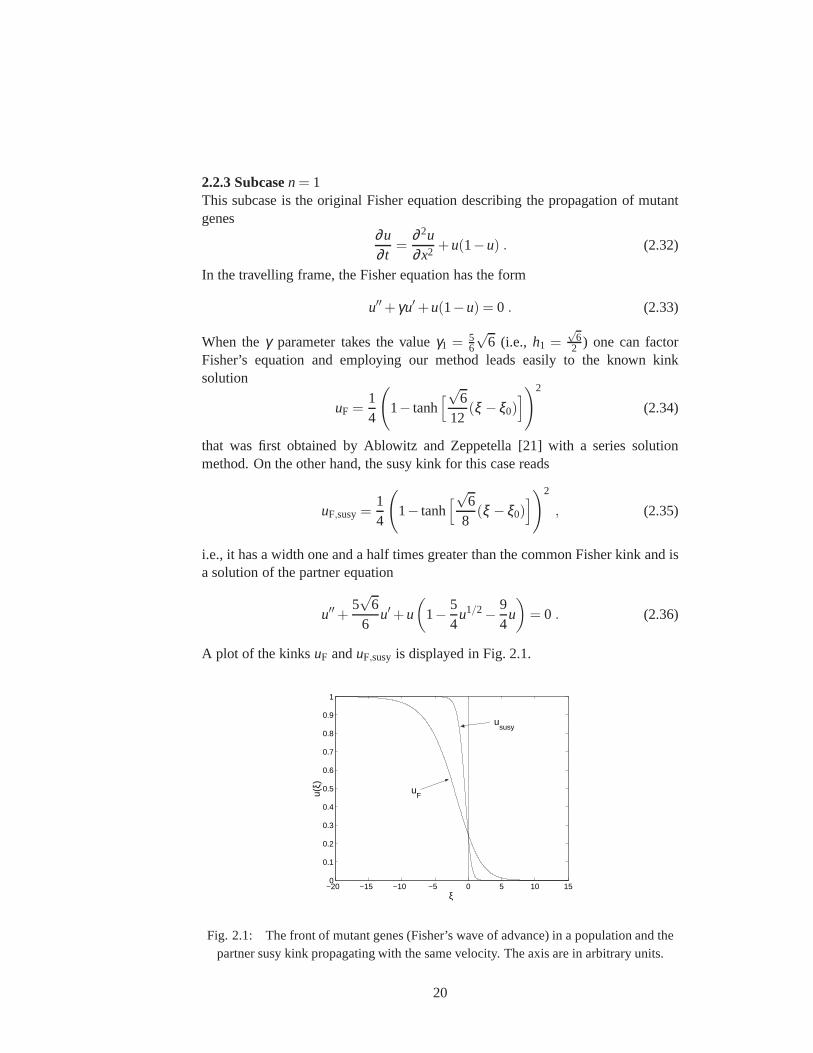
A plot of the kinksuF anduF,susy is displayed in Fig. 2.1.

−20 −15 −10 −5 0 5 10 150

0.1

0.2

0.3

0.4

0.5

0.6

0.7

0.8

0.9

1

ξ

u(ξ)

ususy

uF

Fig. 2.1: The front of mutant genes (Fisher’s wave of advance) in a population and thepartner susy kink propagating with the same velocity. The axis are in arbitrary units.

20

2.2.4 Subcasen= 6This subcase is of interest in the light of experiments on polymerization patternsof MTs in centrifuges. It has been discovered that the polymerization of thetubulin dimers proceeds in a kink-switching fashion propagating with a constantvelocity within the sample. Portet, Tuszynski and Dixon [20] used RD equationsto discuss the modification of self-organization patterns of MTs as well as thetubulin polymerization under the influence of reduced gravitational fields. Theyused the valuen= 6 for the mean critical number of tubulin dimers at which thepolymerization process starts and showed that the same nucleation number entersthe polynomial term of the RD process for the number concentration c of tubulindimers

c′′+52

c′+c(

1−c6)= 0 . (2.37)

The polymerization kink in their work reads

cPTD = 2−13

(

1− tanh[3

4(ξ −ξ0)

]

)1/3

. (2.38)

On the other hand, the susy polymerization kink (see Fig. (2.2)) of the form

csusy= 2−13

(

1− tanh[3(ξ −ξ0)])1/3

(2.39)

can be taken into account according to the hyperbolic form ofEq. (2.30). Itpropagates with the same speed and corresponds to the equation

c′′± 52

c′+c(

1−15c3−16c6)= 0 . (2.40)

In principle, this equation could be obtained as a consequence of modifying thekinetics steps in the microtubule polymerization process.

−5 0 5 10 150

0.1

0.2

0.3

0.4

0.5

0.6

0.7

0.8

0.9

1

ξ

C(ξ

)

Tubulin

MT’s

Vwave front

CPTD

Csusy

Fig. 2.2: The polymerization kink of Portet, Tuszynski and Dixon [20] and the susykink propagating with the same velocity.

21

2.3 Equations of the Dixon-Tuszynski-Otwinowski type

In the context of damped anharmonic oscillators, Dixon et al. [22] studiedequations of the type (in this section, we use′ = Dτ =

ddτ )

u′′+u′+Au−un−1 ≡ u′′+u′+u(√

A−un2−1)(

√A+u

n2−1) = 0 (2.41)

and gave solutions for the casesA = 29 and A = 3

16, with n = 4 and n = 6,respectively. For this case, time is the independent variable. The factorizationmethod works nicely if one usesgn =

√

n/2 and dealing with the more generalequation

u′′±√

A(gn+g−1n )u′+u(A−un−2) = 0, (2.42)

for which we can employ either the factorization functions

φ1 =∓g−1n

(√A−u

n2−1)

, φ2 =∓gn

(√A+u

n2−1)

or

φ1 =∓g−1n

(√A+u

n2−1)

, φ2 =∓gn

(√A−u

n2−1)

.

Then, Eq. (2.42) can be factored in the forms[

Dτ ±gn(un2−1+

√A)][

Dτ ∓g−1n (u

n2−1−

√A)]

u= 0 (2.43)

and[

Dτ ∓gn(un2−1−

√A)][

Dτ ±g−1n (u

n2−1+

√A)]

u= 0 . (2.44)

Thus, Eq. (2.42) is compatible with the equations

u′∓g−1n

(

un2−1−

√A)

u= 0, (2.45)

u′±g−1n

(

un2−1+

√A)

u= 0 (2.46)

that follows from Eq. (2.43) and Eq. (2.44). Integration of Eqs. (2.45), (2.46) givesthe solution of Eq. (2.42)

u> =

√A

1±exp[√

A(gn−g−1n )(τ − τ0)

]

2n−2

, γ > 0 (2.47)

and

u< =

√A

1±exp[

−√

A(gn−g−1n )(τ − τ0)

]

2n−2

, γ < 0 . (2.48)

22

The solutions obtained by Dixon et al. are particular cases of the latter formulas.Reversing now the factorization brackets in (2.43)

[

Dτ ∓g−1n

(

un2−1−

√A)][

Dτ ±gn(un2−1+

√A)]

u= 0 (2.49)

leads to the following equation

u′′±√

A(gn+g−1n )u′+u

(√A+u

n2−1)

(√A− n2

4u

n2−1)

= 0, (2.50)

which is compatible with the equation

u′±gn

(

un2−1+

√A)

u= 0 (2.51)

whose integration gives the solution of Eq. (2.50)

u> =

( √A

1±exp[√

Agn(τ − τ0)]

) 2n−2

, γ > 0 (2.52)

and

u< =

( √A

1±exp[−√

Agn(τ − τ0)]

) 2n−2

, γ < 0 . (2.53)

2.4 FitzHugh-Nagumo equation

Let us consider the FitzHugh-Nagumo equation, which is a common approxima-tion to describe nerve fiber propagation,

∂u∂ t

− ∂ 2u∂x2 +u(1−u)(a−u) = 0 , (2.54)

where a is a real constant. Moreover, ifa = −1, one gets the real Newell-Whitehead equation describing the dynamical behavior nearthe bifurcation pointfor the Rayleigh-Bénard convection of binary fluid mixtures. The travelling frameform of (2.54) has been discussed in detail by Hereman and Takaoka [19]

u′′+ γu′+u(u−1)(a−u) = 0. (2.55)

The FitzHugh-Nagumo polynomial function allows the following factorizations:

φ1 =±(√

2)−1(u−1), φ2 =±√

2(a−u)

when theγ parameter is equal toγa1 = ±−2a+1√2

that we also write asγa,1 =

±√a(ga1−g−1

a1 ), wherega1 =−√

2a.

23

In addition, we can employ the factorization functions

φ1 =±(√

2)−1(a−u), φ2 =±√

2(u−1)

whenγa,2 =±−a+2√2

, or written again in the more symmetric formγa,2 =±√a(ga2−

g−1a2 ), wherega2 =−

√

a/2. Thus, Eq. (2.55) can be factored in the two cases

u′′± γa,1u′+u(u−1)(a−u) = 0, (2.56)

andu′′± γa,2u′+u(u−1)(a−u) = 0 . (2.57)

In passing, we notice that for the Newell-Whitehead casea=−1 the two equationscoincide and are the same as the generalized Fisher equationfor n= 2.In factorization bracket forms, Eqs. (2.56) and (2.57) are written as follows

[

D∓√

2(a−u)][

D± (√

2)−1(1−u)]

u= 0 (2.58)

and[

D∓√

2(u−1)][

D∓ (√

2)−1(a−u)]

u= 0, (2.59)

and are compatible with the first order differential equations

u′± (√

2)−1(1−u)u= 0, for γa,1 , (2.60)

u′∓ (√

2)−1(a−u)u= 0, for γa,2 . (2.61)

Integration of Eqs. (2.60) and (2.61) gives the solution of Eq. (2.55) for the twodifferent values of the wave front velocityγa,1 andγa,2.For Eq. (2.56) we get

u> =1

1±exp[(√

2)−1(ξ −ξ0)], u< =

1

1±exp[−(√

2)−1(ξ −ξ0)], (2.62)

for γa,1 positive and negative, respectively.As for Eq. (2.57), the solutions are

u> =a

1±exp[−(√

2)−1a(ξ −ξ0)], u< =

a

1±exp[(√

2)−1a(ξ −ξ0)], (2.63)

for γa,2 positive and negative, respectively.Considering now the factorizations (2.58) and (2.59), the change of order of thefactorization brackets gives

[

D± (√

2)−1(1−u)][

D∓√

2(a−u)]

u= 0 (2.64)

and[

D∓ (√

2)−1(a−u)][

D∓√

2(u−1)]

u= 0 . (2.65)

24

Doing the product of differential operators (and considering the factorization termu′−φ2u= 0) gives the following RD equations

u′′± γa1u′+u(4u−1)(a−u) = 0, (2.66)

andu′′± γa2u′+u(u−1)(a−u−3u2) = 0, (2.67)

Eqs. (2.66) and (2.67) are compatible with the equations

u′∓√

2(a−u)u= 0 (2.68)

andu′∓

√2(u−1)u= 0 , (2.69)

respectively. Integrations of Eqs. (2.68) and (2.69) give the solutions of Eqs. (2.66)and (2.67), respectively. The explicit forms are the following:(i) for (2.66)

u> =a

1±exp[−√

2a(ξ −ξ0)], u< =

a

1±exp[√

2a(ξ −ξ0)]. (2.70)

(ii) for (2.67)

u> =1

1±exp[√

2(ξ −ξ0)], u< =

1

1±exp[−√

2(ξ −ξ0)]. (2.71)

2.5 Conclusion of the chapter

In this chapter, we have been concerned with stating an efficient factorizationscheme of ODE with polynomial nonlinearities that leads to an easy finding ofanalytical solutions of the kink type that previously have been obtained by farmore cumbersome procedures. The main result is an interesting pairing betweenequations with different polynomial nonlinearities, which is obtained by applyingthe susy quantum mechanical reverse factorization. The kinks of the two nonlinearequations are of different widths but they propagate at the same velocity, or ifwe deal with damped polynomial nonlinear oscillators the two kink solutionscorrespond to the same friction coefficient. Several important cases, such asthe generalized Fisher and the FitzHugh-Nagumo equations,have been shown tobe simple mathematical exercises for this factorization technique. The physicalprediction is that for commonly occurring propagating fronts, there are two kinkfronts of different widths at a given propagating velocity.Moreover, the reversefactorization procedure can be also applied to the Berkovich scheme with similarresults. It will be interesting to apply the approach of thiswork to the discretecase in which various exact results have been obtained in recent years [23]. Moregeneral cases in which the coefficientγ is an arbitrary function are also of muchinterest because of possible applications. The same factorization scheme as itworks for more complicated ordinary differential equations is described in the nextchapter.

25

3Application to more general nonlinear differentialequations

Abstract. In the previous chapter we considered the coefficient in front of the firstderivative as a constant quantity. However, the employed factorization technique can beused almost unchanged for the more general case when the condition of constancy of thiscoefficient is relaxed. In this chapter, we obtain more kink type solutions through thesame factorization procedure for a number of more general nonlinear ordinary second orderdifferential equations with important applications in biology and physics.

3.1 Introduction

Considering the following type of differential equation

u′′+g(u)u′+F(u) = 0 (3.1)

where again as in the previous chapter′ means the derivativeD= ddξ andξ = x−vt;

one can factorize Eq. (3.1) in the following form

[D−φ2(u)] [D−φ1(u)]u= 0. (3.2)

Performing now the product of differential operators leadsto the equation

u′′− dφ1

duuu′−φ1u′−φ2u′+φ1φ2u= 0, (3.3)

for which one way of grouping the terms is as follows

u′′−(

φ1+φ2+dφ1

duu

)

u′+φ1φ2u= 0. (3.4)

26

Eqs. (3.1) and (3.4) are lead to the conditions

g(u) =−(

φ1+φ2+dφ1

duu

)

(3.5)

and

F(u) = φ1φ2u . (3.6)

If F(u) is a polynomial function, theng(u) will have the same order as the biggerof the factorizing functionsφ1(u) and φ2(u), and will also be a function of theconstant parameters provided by the functionF(u).In the context of classical mechanics, Eq. (3.1) could be seen as an anharmonicoscillator with nonlinear damping. The caseg(u) = ν where ν is a constantvalue has been presented in the previous chapter. There, by means of asimple factorization method exact particular solutions ofthe kink type forreaction-diffusion equations and damped-anharmonic oscillators with polynomialnonlinearities have been obtained. In addition, SUSYQM-like reversing offactorization brackets has been performed providing new kink solutions forequations with different polynomial nonlinearities.Based on the given grouping in Eq. (3.4) for Eq. (3.1), a simple mathematicalprocedure is proposed by which one gets particular solutions through factorizationmethods that allows finding solutions satisfying a compatible (nonlinear) first orderdifferential equation.The purpose of this chapter is to further apply this mathematical scheme to a wealthof important cases for which explicit particular solutionsare not easy to find in theliterature or are obtained by more involved techniques. Theexamples we presentherein are the modified Emden equation, the Generalized Lienard equation, theconvective Fisher equation, the generalized Burgers-Huxley equation, all of whomhave significant applications in nonlinear physics. Explicit particular solutions arepresented.

3.2 Modified Emden equation

Let us consider the following modified Emden equation

u′′+αuu′+βu3 = 0 . (3.7)

The polynomialF(u) = βu3 allows the following factorizing functions

φ1(u) = a1

√

βu , and φ2(u) =1a1

√

βu , a1 6= 0 ,

wherea1 is an arbitrary constant. Eq. (3.5) is used to obtain the function g(u),

g(u) =−(

2a1

√

βu+1a1

√

βu

)

=−√

β(

2a21+1a1

)

u ,

27

then identifyingα =−√

β(

2a21+1a1

)

(or a1+,− =−α±

√α2−8β

4√

β), where we usea1 as

a fitting parameter providing thata1 < 0 for α > 0. We note thatg(u) = g(β ,a1;u).Eq. (3.7) is now rewritten in the following form

u′′−√

β(

2a21+1a1

)

uu′+βu3 = 0 , (3.8)

the equation can be factorized as follows

(

D− 1a1

√

βu

)

(

D−a1

√

βu)

u= 0 (3.9)

and therefore the compatible first order differential equation is

u′−a1

√

βu2 = 0 . (3.10)

Integration of Eq. (3.10) gives the particular solution of Eq. (3.8)

u=− 1

a1√

β (ξ −ξ0), (3.11)

whereξ0 is an integration constant. If we consider the quadratic equation fora1,then Eq. (3.11) is expressed as a function ofα ,

u=4

(α ±√

α2−8β )(ξ −ξ0). (3.12)

-10

-5

0

5

10

Α-10

-5

0

5

10

Β

-1

-0.5

0

0.5

1

a1

-10

-5

0

5

10

Α

Fig. 3.1: Real part for the factorization curve of the parametera1+ = a1+(α,β ) thatallows the factorization of Eq. (3.8).a1 6= 0. α ∈ [−10,10] andβ ∈ [−10,10].

28

-10

-5

0

5

10

Α-10

-5

0

5

10

Β

-4

-2

0

a1

-10

-5

0

5

10

Α

Fig. 3.2: Imaginary part for the factorization curve of the parametera1+ = a1+(α,β ) thatallows the factorization of Eq. (3.8).a1 6= 0. α ∈ [−10,10] andβ ∈ [−10,10].

Let us consider now another pair of factorizing functions

φ1(u) = a1

√

βu2, φ2(u) =1a1

√

β ,

then, using Eq. (3.5), the functiong(u) = −√

β(

1a1+3a1u2

)

is easily obtained.

Therefore, the original modified Emden equation (3.7) becomes

u′′−√

β(

1a1

+3a1u2)

u′+βu3 = 0 . (3.13)

This equation allows the factorization

(

D− 1a1

√

β)

(

D−a1

√

βu2)

u= 0 , (3.14)

where from we obtain the compatible first order differentialequation

u′−a1

√

βu3 = 0 (3.15)

with the solution

u=1

[−2a1

√

β (ξ −ξ0)]1/2. (3.16)

The above example shows that different factorizations ofF(u) would yield differ-ent forms for the functiong(u). This is an important consequence of applying thismathematical technique to the caseg(u) 6= const.

29

3.3 Generalized Lienard equation

Let us consider now the following generalized Lienard equation with a cubicpolynomial functionF(u)

u′′+g(u)u′+Au+Bu2+Cu3 = 0 . (3.17)

The polynomial functionF(u) can be factorized in several ways, we consider firstthe factorizationF(u) = u(a+b+Cu)(d−e+u) where

a= B/2, b=√

B2−4AC/2, d = B/2C, e=√

B2−4AC/2C,

and the conditionB2−4AC> 0 holds. If we consider the factorizing functions as

φ1(u) = a1(a+b+Cu) and φ2(u) =1a1

(d−e+u) ,

where againa1 is an arbitrary constant that can be used as a fitting parameter, the

functiong(u) =[

a21(a+b)+(d−e)

a1+(

2a21C+1a1

)

u]

will be obtained. Then, Eq. (3.17) is

rewritten as

u′′+

[

a21(a+b)+ (d−e)

a1+

(

2a21C+1a1

)

u

]

u′+Au+Bu2+Cu3 = 0 , (3.18)

and the corresponding factorization will be[

D− 1a1

(d−e+u)

]

[D−a1(a+b+Cu)]u= 0 (3.19)

where from the compatible first order differential equationis obtained

u′−a1(a+b+Cu)u= 0 , (3.20)

and whose solution is

u=(a+b)exp[a1(a+b)(ξ −ξ0)]

1−Cexp[a1(a+b)(ξ −ξ0)](3.21)

where(a+b) = B+√

B2−4AC2 .

Let us consider now the following reduction of terms in Eq. (3.17),B= 0 andC= 1in order to calculate a particular solution for the so-called autonomous Duffing-vander Pol oscillator equation [25],

u′′+(G+Eu2)u′+Au+u3 = 0 , (3.22)

whereG andE are arbitrary constant parameters. The polynomial function allowsthe following factorizing functions

f1(u) = a1(A+u2) and φ2(u) =1a1

,

30

theng(u) =−(

a21A+1a1

+3a1u2)

. Eq. (3.22) is now rewritten

u′′−(

a21A+1

a1+3a1u2

)

u′+Au+u3 = 0 . (3.23)

The corresponding factorization of Eq. (3.23) is given as follows[

D− 1a1

]

[

D−a1(A+u2)]

u= 0 , (3.24)

and the obtained compatible first order equation

u′−a1(A+u2)u= 0 . (3.25)

Integration of Eq. (3.25) gives the particular solution of Eq. (3.23)

u=√

A

(

exp[2a1A(ξ −ξ0)]

1−exp[2a1A(ξ −ξ0)]

)1/2

. (3.26)

Comparing Eqs. (3.22) and (3.23),a1 =−E3 andG= AE2+9

3E are obtained. Solution(3.26) is now written as a function ofA andE,

u=±√

A

(

exp[−23AE(ξ −ξ0)]

1−exp[−23AE(ξ −ξ0)]

)1/2

. (3.27)

This is a more general result for the particular solution than that obtained by Chan-drasekar et al. in [25] by other means, in fact, it is recuperated whenE = β andA= 3

β2 .

-10

-5

0

5

10

G

-10

-5

0

5

10

A

-10

-5

0

5

10

E

-10

-5

0

5

10

G

Fig. 3.3: Real part for the factorization curve of the parameterE+ = E+(G,A) that allowsthe factorization of Eq. (3.23). Note thata1 =−E

3 ; E 6= 0. G∈ [−10,10] andA∈ [−10,10].

31

-10

-5

0

5

10

G

-10

-5

0

5

10

A

0

0.5

1

1.5

E

-10

-5

0

5

10

G

Fig. 3.4: Imaginary part for the factorization curve of the parameterE+ = E+(G,A) thatallows the factorization of Eq. (3.23).E 6= 0. G∈ [−10,10] andA∈ [−10,10].

3.4 Convective Fisher equation

Let us consider the convective Fisher equation given in the following form [26],

∂u∂ t

=12

∂ 2u∂x2 +u(1−u)−µu

∂u∂x

(3.28)

where µ is a positive parameter that serves to tune the relative strength ofconvection. If the variable transformationξ = x−νt is performed, then we obtainthe following ordinary differential equation

u′′+2(ν −µu)u′+2u(1−u) = 0 . (3.29)

The polynomial function allows the factorizing functions

φ1(u) =√

2a1(1−u) and φ2(u) =

√2

a1,

and Eq. (3.5) gives the functiong(u) = −√

2(

a21+1a1

−2a1u)

. Eq. (3.29) is

rewritten as follows

u′′+2

(

−a21+1√2a1

+√

2a1u

)

u′+2u(1−u) = 0 . (3.30)

If we set the fitting parametera1 = − µ√2, then we obtainν = µ2+2

2µ . Eq. (3.30) isfactorized in the following form

[

D−√

2a1

]

[

D−√

2a1(1−u)]

u= 0 , (3.31)

32

that provides the compatible first order equation

u′−√

2a1u(1−u) = u′+µu(1−u) = 0 (3.32)

whose integration gives

u=1

1±exp[µ(ξ −ξ0)]. (3.33)

0 2 4 6 8 10 12 14Μ

0

2

4

6

8

10

12

14

ΝHΜL

Fig. 3.5: Factorization curve of the parameterν = ν(µ) that allows the factorization ofEq. (3.30).a1 =− µ√

2.

3.5 Generalized Burgers-Huxley equation

In this section we obtain particular solutions for the generalized Burgers-Huxleyequation discussed by Wang et al. in [27]

∂u∂ t

−αuδ ∂u∂x

− ∂ 2u∂x2 = βu(1−uδ )(uδ − γ) . (3.34)

If the coordinates transformationξ = x− νt is performed then Eq. (3.34) isrewritten in the following form

u′′+(ν +αuδ )u′+βu(1−uδ )(uδ − γ) = 0 , (3.35)

and the polynomial function allows the choice for the factorizing terms

φ1(u) =√

βa1(1−uδ ) and φ2(u) =

√

βa1

(uδ − γ) .

Eq. (3.5) providesg(u) =√

β(

γ−a21

a1+

a21(1+δ )−1

a1uδ)

, and we can do the following

identification of constant parameters

ν =√

β(

γ −a21

a1

)

, α =√

β(−a2

1(1+δ )+1a1

)

.

33

Writing Eq. (3.35) in factorized form

[

D−√

βa1

(uδ − γ)

]

[

D−√

βa1(1−uδ )]

u= 0 , (3.36)

the solution

u=

(

1

1±exp[−a1

√

βδ (ξ −ξ0)]

)1/δ

(3.37)

of the compatible first order equation

u′−√

βa1u(1−uδ ) = 0 , (3.38)

is also a particular kink solution of Eq. (3.35). Solving thequadratic equation(3.36) fora1 = a1(α ,β ,δ ) we obtain

a1+,− =−α ±

√

α2+4β (1+δ )2√

β (1+δ ),

then Eq. (3.37) becomes a functionu= u(α ,β ,δ ;τ), andν = ν(α ,β ,γ ,δ ). If wesetδ = 1 in Eq. (3.34), then we obtain the following particular Burgers-Huxleysolution

u=1

1±exp[−a1

√

β (ξ −ξ0)], (3.39)

anda1+,− =−α±

√α2+8β

4√

β, ν = ν(α ,β ,γ).

-20

-10

0

10

20

Α

-20

-10

0

10

20

Β

2468

10

a1

-20

-10

0

10

20

Α

Fig. 3.6: Real part for the factorization curve of the parametera1+ = a1+(α,β ,δ = 1) thatallows factorization of Eq. (3.35) withδ = 1. a1 6= 0. α ∈ [−20,20] andβ ∈ [−20,20].

34

-20

-10

0

10

20

Α

-20

-10

0

10

20

Β

-1

-0.5

0

0.5

a1

-20

-10

0

10

20

Α

Fig. 3.7: Imaginary part for the factorization curve of the parametera1+ = a1+(α,β ,δ = 1) that allows factorization of Eq. (3.35) withδ = 1. a1 6= 0.

α ∈ [−20,20] andβ ∈ [−20,20].

If we chose now the factorizing terms as

φ1(u) =√

βe1(uδ − γ) and φ2(u) =

√

βe1

(1−uδ ) ,

we obtain g(u) =√

β(

e21γ−1e1

+1−e2

1(1+δ )e1

uδ)

, and the following identification

of parametersν =√

β(

e21γ−1e1

)

and α =√

β(

1−e21(1+δ )e1

)

. Eq. (3.35) is then

factorized in the different form[

D−√

βe1

(1−uδ )

]

[

D−√

βe1(uδ − γ)

]

u= 0 . (3.40)

The corresponding compatible first order equation is now

u′−√

βe1u(uδ − γ) = 0 , (3.41)

and its integration gives a different particular solution for Eq. (3.35) from thatobtained for the first choice of factorizing terms (3.36), however, we point outthat the parameterα has changed for the second choice of factorizing terms. Thesolution of Eq. (3.41) is given as follows

u=

(

γ1±exp[±e1

√

βγδ (ξ −ξ0)]

)1/δ

. (3.42)

Solving the quadratic equation fore1 = e1(α ,β ,δ ) we obtain

e1+,− =α ±

√

α2+4β (1+δ )2√

β (1+δ ),

35

then Eq. (3.42) becomesu= u(α ,β ,γ ,δ ;τ), andν = ν(α ,β ,γ ,δ ). If we setδ = 1in Eq. (3.34), then the following Burgers-Huxley solution is obtained

u=γ

1±exp[e1√

βγ(ξ −ξ0)], (3.43)

ande1+,− =α±

√α2+8β

4√

β, ν = ν(α ,β ,γ).

-20

-10

0

10

20

Α

-20

-10

0

10

20

Β

0

1

2

3e1

-20

-10

0

10

20

Α

Fig. 3.8: Real part for the factorization curve of the parametere1+ = e1+(α,β ,δ = 1) thatallows factorization of Eq. (3.35) withδ = 1. e1 6= 0. α ∈ [−20,20] andβ ∈ [−20,20].

-20

-10

0

10

20

Α

-20

-10

0

10

20

Β

-1

-0.5

0

0.5

e1

-20

-10

0

10

20

Α

Fig. 3.9: Imaginary part for the factorization curve of the parametere1+ = e1+(α,β ,δ = 1) that allows factorization of Eq. (3.35) withδ = 1. e1 6= 0.

α ∈ [−20,20] andβ ∈ [−20,20].

Eqs. (3.37) and (3.42) representing particular solutions for the GBHE, are the sameas those obtained by Wang et al. [27].

36

3.6 Conclusion of the chapter

In this chapter, we apply the same factorization scheme for more complicatedsecond order nonlinear differential equations as in Chapter 2. Exact particularsolutions have been found for a series of nonlinear differential equations withapplications in physics and biology: the modified Emden equation, the generalizedLienard equation, the Duffing-van der Pol equation, the convective Fisher equation,and the generalized Burgers-Huxley equation. Also, we display parametric curvesalong which the differential equations under consideration could be factorized. Wefind that the proposed factorization procedure is easier andmore efficient than othermethods used to find particular solutions of second order differential equations.

37

4One-parameter supersymmetry for microtubules

Abstract. The simple supersymmetric model of Caticha [34] as used by Rosu [33] todescribe the motion of ferrodistortive domain walls in microtubules (MTs), is generalizedto the case of Mielnik’s one-parameter nonrelativistic supersymmetry [11]. By this means,one can introduce Montroll double-well potentials with singularities that move along thepositive or negative travelling direction depending on thesign of the free parameter ofMielnik’s method. Possible interpretations of the singularity are microtubule associatedproteins (motors) or structural discontinuities in the arrangement of the tubulin molecules.

4.1 Introduction

Based on well-established results of Collins, Blumen, Currie and Ross [29] regardingthe dynamics of domain walls in ferrodistortive materials,Tuszynski and collaborators[30, 31] considered MTs to be ferrodistortive and studied kinks of the Montroll type [32]as excitations responsible for the energy transfer within this highly interesting biologicalcontext.The Euler-Lagrange dimensionless equation of motion of ferrodistortive domain walls asderived in [29] from a Ginzburg-Landau free energy with driven field and dissipationincluded is of the travelling reaction-diffusion type

ψ′′+ρψ

′ −ψ3+ψ +σ = 0 , (4.1)

where the primes are derivatives with respect to a travelling coordinateξ = x− vt, ρ is afriction coefficient andσ is related to the driven field [29].There may be ferrodistortive domain walls that can be identified with the Montroll kinksolution of Eq. (4.1)

M(ξ ) = α1+

√2β

1+exp(β ξ ), (4.2)

whereβ = (α2−α1)/√

2 and the parametersα1 andα2 are two nonequal solutions of thecubic equation

(ψ −α1)(ψ −α2)(ψ −α3) = ψ3−ψ −σ . (4.3)

38

4.2 Caticha’s supersymmetric model as applied to MTs

Rosu has noted that Montroll’s kink can be written as a typical tanh kink [33]

M(ξ ) = γ − tanh

(

β ξ2

)

, (4.4)

where γ ≡ α1 + α2 = 1+ α1√

2β . The latter relationship allows one to use a simple

construction method of exactly soluble double-well potentials in the Schrödinger equationproposed by Caticha [34]. The scheme is a non-standard application of Witten’ssupersymmetric quantum mechanics [9] having as the essential assumption the idea ofconsidering theM kink as the switching function between the two lowest eigenstates of theSchrödinger equation with a double-well potential. Thus

φ1 = Mφ0 , (4.5)

whereφ0,1 are solutions ofφ ′′0,1 + [ε0,1 − u(ξ )]φ0,1(ξ ) = 0, andu(ξ ) is the double-well

potential to be found. Substituting Eq. (4.5) into the Schrödinger equation for the subscript1 and substracting the same equation multiplied by the switching function for the subscript0, one obtains

φ′0+RMφ0 = 0 , (4.6)

whereRM is given by

RM =M

′′+ εM

2M′ , (4.7)

andε = ε1 − ε0 is the lowest energy splitting in the double-well Schrödinger equation.In addition, notice that Eq. (4.6) is the basic equation introducing the superpotentialR inWitten’s supersymmetric quantum mechanics, i.e., the Riccati solution. For Montroll’skink the corresponding Riccati solution reads

RM(ξ ) =−β2

tanh

(

β2

ξ)

+ε

2β

[

sinh(β ξ )+2γ cosh2(

β2

ξ)

]

(4.8)

and the ground-state Schrödinger function is found by meansof Eq. (4.6)

φ0,M(ξ ) = φ0(0)cosh

(

β2

ξ)

exp

(

ε2β 2

)

exp

(

− ε2β 2

[

cosh(β ξ )

−γβ ξ − γ sinh(β ξ )])

, (4.9)

while φ1 is obtained by switching the ground-state wave function by means ofM. Thisground-state wave function is of supersymmetric type

φ0,M(ξ ) = φ0,M(0)exp

[

−∫ ξ

0RM(y)dy

]

, (4.10)

whereφ0,M(0) is a normalization constant.

39

The Montroll double well potential is determined up to the additive constantε0 by the‘bosonic’ Riccati equation

uM(ξ ) = R2M −R

′M + ε0 =

β 2

4+

(γ2−1)ε2

4β 2 +ε2+ ε0

+ε

8β 2

[

(

4γ2ε +2(γ2+1)εcosh(β ξ )−8β 2)cosh(β ξ )

−4γ(

ε + εcosh(β ξ )−2β 2)sinh(β ξ )]

. (4.11)

Plots of the asymmetric Montroll potential and ground statewave function are given inFigs. 4.1 and 4.2 for a particular set of the parameters. If, as suggested by Caticha, onechooses the ground state energy to be

ε0 =−β 2

4− ε

2+

ε2

4β 2

(

1− γ2) , (4.12)

then uM(ξ ) turns into a travelling, asymmetric Morse double-well potential of depthsdepending on the Montroll parametersβ andγ and the splittingε

UL,R0,m = β 2

[

1± 2εγ(2β )2

]

, (4.13)

where the subscriptmstands for Morse and the superscriptsL andR for left and right well,respectively. The difference in depth, the bias, is∆m ≡UL

0 −UR0 = 2εγ, while the location

of the potential minima on the travelling axis is at

ξ L,Rm =∓ 1

βln

[

(2β )2±2εγε(γ ∓1)

]

, (4.14)

that shows thatγ 6=±1.

4.3 The Mielnik extension

We now discuss shortly in this context the Mielnik extensionof these results [11, 3]. Thepoint is thatRM in Eq. (4.8) is only the particular solution of Eq. (4.11). The generalsolution is a one-parameter function of the form

RM(ξ ;λ ) = RM(ξ )+d

dξ

[

ln(IM(ξ )+λ )]

(4.15)

and the corresponding one-parameter Montroll potential isgiven by

uM(ξ ;λ ) = uM(ξ )−2d2

dξ 2

[

ln(IM(ξ )+λ )]

. (4.16)

In these formulas,IM(ξ ) =∫ ξ φ2

0,M(ξ )dξ and λ is an integration constant that is usedas a deforming parameter of the potential and is related to the irregular zero mode. Theone-parameter Darboux-deformed ground state wave function can be shown to be

φ0,M(ξ ;λ ) =√

λ (λ +1)φ0,M

IM(ξ )+λ, (4.17)

40

where√

λ (λ +1) is the normalization factor implying thatλ /∈ [0,−1]. Moreover, theMielnik parametric potentials and wave functions display singularities atλs = −IM(ξs).Plots ofuM(ξ ;λ ) andφ0,M(ξ ;λ ) for λ = 1,10,100 are presented in Figs. 4.3-4.12 and areuseful to see the behavior of the singularities and the deformation effect of theλ parameter.For large values of±λ the singularity moves towards∓∞ and the potential and ground statewave function recover the shapes of the non-parametric potential and wave function as canbe seen in Figs. 4.11 and 4.12, respectively. The one-parameter Morse case correspondsformally to the change of subscriptM → m in Eqs. (4.15) and (4.16). For the single wellMorse potential the one-parameter procedure has been studied by Filho [35] and Bentaibaet al [36].Mielnik’s approach leads to singularities in the double-well potential and the correspondingwave functions. If the parameterλ is positive the singularity is to be found on thenegativeξ axis, while for negativeλ it is on the positive side. Potentials and wavefunctions with singularities are not so strange as it seems [37] and could be quite relevanteven in nanotechnology [38] where quantum singular interactions of the contact typeare appropriate for describing nanoscale quantum devices.We interpret the singularityas representing the effect of an impurity moving along the MTin one direction or theother depending on the sign of the parameterλ . The impurity may represent a proteinattached to the MT or a structural discontinuity in the arrangement of the tubulin molecules.This interpretation of impurities has been given by Trpišová and Tuszynski in non-supersymmetric models of nonlinear MT excitations [39].

4.4 Conclusion of the chapter

In conclusion, the supersymmetric approaches allow for a number of interestingexactresults in this biological framework and point to a direct connection between Schrödingerdouble-well potentials and nonlinear kinks encountered innonequilibrium chemicalprocesses. MTs are an important application but the procedures described here can be usedin many other applications. Moreover, the supersymmetric constructions can be used as abackground for clarifying further details of the exact models. Although it is not so clearwhy one should take a certain type of kink as switching function between the Schrödingersplit modes, it is interesting that proceeding in this way one will be led to some familiardouble-well potentials in chemical physics.

41

-4 -2 2 4

-2

2

4

6

8

10

Fig. 4.1: The Montroll asymmetric double-well potential (MDWP) calculated usingEq. (4.11) forε0 = 0. In all figuresα1 = 1, α2 =−1.5, β =−2.5/

√2, γ =−0.5, ε = 0.1.

-4 -2 2 4

0.5

1

1.5

2

2.5

3

3.5

Fig. 4.2: The Montroll ground state wave function cf Eq. (4.9) for φ0(0) = 1.

-4 -2 2 4

50

100

150

Fig. 4.3: The one-parameter Darboux modified MDWP forλ = 1.

42

-2.8 -2.6 -2.4 -2.2 -2 -1.8 -1.6

1

2

3

4

5

Fig. 4.4: The low-scale left hand side of the singularity.

0.5 1 1.5 2 2.5 3 3.5

-0.2

0.2

0.4

Fig. 4.5: The low-scale right hand side of the singularity.

-4 -2 2 4

-15

-10

-5

5

10

15

Fig. 4.6: The wave functions forλ = 1.

43

-4 -2 2 4

-5

5

10

15

20

Fig. 4.7: One parameter Darboux-modified MDWP forλ = 10 .

0.5 1 1.5 2 2.5 3 3.5

-1

-0.5

0.5

1

Fig. 4.8: The bottom of the potential at the right hand side.

-3 -2 -1 1 2 3 4

1

2

3

4

Fig. 4.9: The ground state wave function corresponding toλ = 10.

44

-10 -5 5 10

-5

5

10

15

20

Fig. 4.10: Plot of the integralIM(ξ ) that produces the deformation of the potential andwave functions.

45

5Supersymmetric method with Dirac parameters

Abstract. In this chapter we first describe a "supersymmetric" one-dimensional matrixprocedure similar to relationships of the same type betweenDirac and Schrödingerequations in particle physics that we apply to two problems in classical mechanics andquantum mechanics, respectively. In the first case, we obtain a class of parametricoscillation modes that we call K-modes with damping and absorption that are connectedto the classical harmonic oscillator modes through this supersymmetric procedure that ischaracterized by coupling parameters. When a single coupling parameter, denoted by K,is used, it characterizes both the damping and the dissipative features of these modes.Generalizations to several K parameters are also possible and lead to analytical results. Ifthe problem is passed to the physical optics (and/or acoustics) context by switching fromthe oscillator equation to the corresponding Helmholtz equation, one may hope to detectthe K-modes as waveguide modes of specially designed waveguides and/or cavities. Inthe second case, the same method is presented in a style appropriate for truly quantummechanical problems and an application to the Morse potential is performed. We obtainthe corresponding nonhermitic Morse problem with possibleapplications to the diffractionon optical lattices.

5.1 Introduction

Factorizations of differential operators describing simple mechanical motion have beenonly occasionally used in the past, although in quantum mechanics the procedure ledto a vast literature under the name of supersymmetric quantum mechanics initiated bya paper of Witten [9]. However, as shown by Rosu and Reyes [40], for the dampedNewtonian free oscillator the factorization method could generate interesting results evenin an area settled more than three centuries ago. In this chapter, we apply some of thesupersymmetric schemes to the basic classical harmonic oscillator. In particular, we showhow a known connection in particle physics between Dirac andSchrödinger equationscould lead in the case of harmonic motion to chirped (i.e., time-dependent) frequencyoscillator equations whose solutions are a class of oscillatory modes depending on one

46

more parameter, denoted in the following by K, besides the natural circular frequencyω0.The parameter K characterizes both the damping and the losses of these "supersymmetric"partner modes. Moreover, we do not limit this study to one K parameter extending it toseveral such parameters still getting analytic results. Guided by mathematical equivalence,possible applications in several areas of physics are identified. Moreover, in the final partof the chapter the same supersymmetric scheme is used in the context of exactly solvablequantum problem of the Morse potential. A nonhermitic version of the Morse problem isintroduced in this way.

5.2 Classical harmonic oscillator: The Riccati approach

The harmonic oscillator can be described by one of the simplest Riccati equation

u′+u2+κω2

0 = 0, κ =±1 , (5.1)

where the plus sign is for the normal case whereas the minus sign is for the up side down

case. Indeed, employing u= w′

w one gets the harmonic oscillator differential equation

w′′+κω2

0w = 0 , (5.2)

with the solutions

wb =

W+ cos(ω0t+ϕ+) if κ = 1W−sinh(ω0t+ϕ−) if κ =−1 ,

where W± andϕ± are amplitude and phase parameters, respectively, which can be ignoredin the following.The particular Riccati solution of Eq. (5.1) are

up =

−ω0tan(ω0t) if κ = 1ω0coth(ω0t) if κ =−1 .

It is well known that the particular Riccati solutions enteras nonoperatorial part in thecommon factorizations of the second-order linear differential equations that are directlyrelated to the Darboux isospectral transformations [13].Thus, for Eq. (5.2) one gets (Dt = d

dt)

(

Dt +up)(

Dt −up)

w = w′′+(−u

′p−u2

p)w = 0 . (5.3)

To fix the ideas, we shall use the terminology of Witten’s supersymmetric quantummechanics and call Eq. (5.3) the bosonic equation. We stresshere that the supersymmetricterminology is used only for convenience and should not be taken literally. Thus, thesupersymmetric partner (or fermionic) equation of Eq. (5.3) is obtained by reversing thefactorization brackets

(

Dt −up)(

Dt +up)

wf = w′′+(u

′p−u2

p)w = w′′+ω2

f (t)w = 0 , (5.4)

which is related to the fermionic Riccati equation

u′ −u2−ω2

f (t) = 0 , (5.5)

47

where the free termω2f is the following function of time

ω2f (t) = u

′p−u2

p =

ω20(−1−2tan2ω0t) if κ = 1

ω20(1−2coth2ω0t) if κ =−1 .

The solutions (fermionic zero modes) of Eq. (5.4) are given by

wf =

−ω0cos(ω0t) if κ = 1

ω0sinh(ω0t) if κ =−1 ,

and thus present strong periodic singularities in the first case and just one singularity at theorigin in the second case. These ‘partner’ oscillators, as well as those to be discussed inthe following, are parametric oscillators, i.e., of time-dependent frequency. Moreover, theirfrequencies can become infinite (periodically). In general, signals of this type are knownas chirps. "Infinite" chirps could be produced, in principle, in very special astrophysicalcircumstances, e.g., close to black hole horizons [41].

5.3 Matrix formulation

Using the Pauli matricesσy =

(

0 −ii 0

)

andσx =

(

0 11 0

)

, we write the matrix

equationD0W ≡ [σyDt +σx(iup)]W = 0 , (5.6)

whereW =

(

w1

w2

)

is a two component spinor. Eq. (5.6) is equivalent to the following

decoupled equations

(iDt + iup)w1 = 0 (5.7)

(−iDt + iup)w2 = 0 . (5.8)

Solving these equations one gets w1 ∝ ω0/cos(ω0t) and w2 ∝ ω0cos(ω0t) for theκ = 1case and w1 ∝ ω0/sinh(ω0t) and w2 ∝ ω0sinh(ω0t) for theκ =−1 case. Thus, we obtain

W =

(

w1

w2

)

=

(

wf

wb

)

. (5.9)

This shows that the matrix equation is equivalent to the two second-order linear differentialequations of bosonic and fermionic type, Eq. (5.2) and Eq. (5.4), respectively, a result quitewell known in particle physics. Indeed, a comparison with the true Dirac equation with aLorentz scalar potential S(x)

[−iσyDx +σx(m+S(x))]W = EW , (5.10)

shows that Eq. (5.6) corresponds to a Dirac spinor of ‘zero mass’ and ‘zero energy’ inan imaginaryscalar ‘potential’ iup(t). We remind that a detailed discussion of the Diracequation in the supersymmetric approach has been provided by Cooper et al [42] in 1988.They showed that the Dirac equation with a Lorentz scalar potential is associated with asusy pair of Schrödinger Hamiltonians. This result has beenused later by many authors inthe particle physics context [43].

48

5.4 Extension through parameterK

We now come to the main issue of this work. Consider the slightly more general Dirac-likeequation

DKW ≡ [σyDt +σx(iup+K)]W = KW , (5.11)

where K is a (not necessarily positive) real constant. On theleft hand side of the equation,K stands as an (imaginary) mass parameter of the Dirac spinor, whereas on the right handside it corresponds to the energy parameter. Thus, we have anequation equivalent to aDirac equation for a spinor of mass iK at the fixed energyE = iK. This equation can bewritten as the following system of coupled equations

iDtw1+(iup+K)w1 = Kw2 (5.12)

−iDtw2+(iup+K)w2 = Kw1 . (5.13)

The decoupling can be achieved by applying the operator in Eq. (5.12) to Eq. (5.13). Forthe fermionic spinor component one gets

D2t w+

1 −ω20

[

(1+2tan2 ω0t)+ i2Kω0

tanω0t]

w+1 = 0 for κ = 1 (5.14)

D2t w−

1 +ω20

[

(1−2coth2ω0t)+ i2Kω0

cothω0t]

w−1 = 0 for κ =−1 , (5.15)

whereas the bosonic component fulfills

D2t w+

2 +ω20

[

1− i2Kω0

tanω0t]

w+2 = 0 for κ = 1 (5.16)

D2t w−

2 −ω20

[

1− i2Kω0

cothω0t]

w−2 = 0 for κ =−1 . (5.17)

The solutions of the bosonic equations are expressed in terms of the Gauss hypergeometricfunctions2F1

w+2 (t;α+,β+) = α+z

(p− 12)

1 z(q− 1

2)2 2F1

[

p+q,p+q−1,2p;−12z1

]

−β+e−2ipπ4(p−12 )z

−(p− 12)

1 z(q− 1

2 )2 2F1

[

q−p,q−p+1,2−2p;−12z1

]

(5.18)

and

w−2 (t;α−,β−) = α−zr

3zs4 2F1

[

r+ s, r+ s+1,1+2r;12

z3

]

+β−4rz−r3 zs

4 2F1

[

s− r+1,s− r,1−2r;12

z3

]

, (5.19)

where the variables zi (i = 1, ...,4) are given in the following form:

z1,2 = i tan(ω0t)∓1, z3,4 = coth(ω0t)±1,

49

respectively. The parameters are the following:

p=12

(

1+

√

1− 2Kω0

)

, q=12

(

1+

√

1+2Kω0

)

,

r =12

√

1+ i2Kω0

, s=12

√

1− i2Kω0

.

The fermionic zero modes can be obtained as the inverse of thebosonic ones. Thus

w+1 =

1

w+2 (t;α+,β+)

, w−1 =

1

w−2 (t;α−,β−)

. (5.20)

A comparison of w+1 with the common 1/cost fermionic mode is displayed in Figs. 5.3and 5.4.In the small K regime, K≪ ω0, one gets

w+2 (t;α+,β+)≈ α+z

(p− 12 )

1 z(q− 1

2 )2 2F1

[

2,1,2− Kω0

;−12

z1(t)]

−

β+e−2ipπ4(p−12 )z

−(p− 12 )

1 z(q− 1

2 )2 2F1

[ Kω0

,1+Kω0

,Kω0

;−12

z1(t)]

(5.21)

and

w−2 (t;α−,β−)≈ α−zr

3zs4 2F1

[

1,2,2+ iKω0

;12

z3(t)]

+

β−4rz−r3 zs

4 2F1

[

1− iKω0

,−iKω0

,−iKω0

;12

z3(t)]

. (5.22)

Examining the bosonic equations, one can immediately see that the resonant frequenciesacquired resistive time-dependent losses whose relative strength is given by the parameterK. The fermionic equations having time-dependent real parts of the frequency canbe interpreted as parametric oscillators which are also affected by losses through theimaginary part.

5.5 More K parameters

A more general case in this scheme is to consider the following matrix Dirac-like equation[

(

0 −ii 0

)

Dt +

(

0 11 0

)(

iup+K1 00 iup+K2

)

]

(

w1

w2

)

=

(

K′1 0

0 K′2

)(

w1

w2

)

. (5.23)

The system of coupled first-order differential equations will be now[

− iDt+ iup+K2

]

w2 = K′1w1 (5.24)

[

iDt + iup+K1

]

w1 = K′2w2 (5.25)

50

and the equivalent second-order differential equations

Dt2wi +

[

− i∆K]

Dtwi +[

±Dtup+ i(K1+K2)up+(K1K2−K′1K

′2)−u2

p

]

wi = 0 , (5.26)

where the subindexi = 1,2 and∆K = K1−K2. Under the gauge transformation

wi = Zi exp

(

−12

∫ t [

− i∆K]

dτ)

= Zi(t)e12 i t∆K , (5.27)

one getsDt

2Zi +Qi(t)Zi = 0, (5.28)

where the ‘potentials’ have the form

Qi(t) =[

±Dtup+ i(K1+K2)up+(K1K2−K′1K

′2)−up

2]

− 14

[

− i∆K]2

(5.29)

Q1,2 are functions that differ from the nonoperatorial parts in Eqs. (5.55)-(5.33) only byconstant terms. Indeed, one can obtain easily the followingequations.For the fermionic spinor component one gets

D2t Z+

1 −ω20

[

1+2tan2 ω0t− (∆K)2

4ω20

− K1K2−K′1K

′2

ω20

+ iK1+K2

ω0tanω0t

]

Z+1 = 0 (5.30)

for κ = 1, and

D2t Z−

1 +ω20

[

1−2coth2ω0t+(∆K)2

4ω20

+K1K2−K

′1K

′2

ω20

+ iK1+K2

ω0cothω0t

]

Z−1 = 0

(5.31)for κ =−1.The bosonic component fulfills

D2t Z+

2 +ω20

[

1+(∆K)2

4ω20

+K1K2−K

′1K

′2

ω20

− iK1+K2

ω0tanω0t

]

Z+2 = 0 , (5.32)

for κ = 1, and

D2t Z−

2 −ω20

[

1− (∆K)2

4ω20

− K1K2−K′1K

′2

ω20

− iK1+K2

ω0cothω0t

]

Z−2 = 0 , (5.33)

for κ =−1. When K1 = K2 = K one gets the particular case studied in full detail above.The more general bosonic modes have the form:

Z+2 (t;α+,β+) = α+[tan(ω0t)− i]

Ω14ω0 [tan(ω0t)+ i]

Ω24ω0

×2F1

[

Ω1+Ω2

4ω0,

Ω1+Ω2

4ω0+1,1+

Ω1

2ω0;12(tan(ω0t)− i)

]

+β+(−1)− Ω1

2ω0 [tan(ω0t)− i]− Ω1

4ω0 [tan(ω0t)+ i]Ω24ω0

×2F1

[

Ω2−Ω1

4ω0,

Ω2−Ω1

4ω0+1,1− Ω1

2ω0;12(tan(ω0t)− i)

]

(5.34)

51

and

Z−2 (t;α−,β−) = α−[coth(ω0t)−1]

Ω34ω0 [coth(ω0t)+1]

Ω44ω0

×2F1

[

Ω3+Ω4

4ω0+1,

Ω3+Ω4

4ω0,1+

Ω3

2ω0;−1

2(coth(ω0t)−1)

]

+β−(−1)− Ω3

2ω0 4Ω32ω0 [coth(ω0t)−1]

− Ω34ω0 [coth(ω0t)+1]

Ω44ω0

×2F1

[

Ω3−Ω4

4ω0,

Ω4−Ω3

4ω0+1,1− Ω3

2ω0;−1

2(coth(ω0t)−1)

]

, (5.35)

where

Ω1 =(

4ω20 +(K1+K2)

2+4[(K1+K2)ω0−K′1K

′2])1/2

,

Ω2 =(

4ω20 +(K1+K2)

2−4[(K1+K2)ω0+K′1K

′2])1/2

,

Ω3 =(

4ω20 − (K1+K2)

2−4[i(K1+K2)ω0−K′1K

′2])1/2

,

Ω4 =(

4ω20 − (K1+K2)

2+4[i(K1+K2)ω0+K′1K

′2])1/2

.

5.6 Possible applications of the K-modes

5.6.1 Waveguides.In view of the correspondence between mechanics and optics,one can also providean interpretation in terms of the Helmholtz optics for lightpropagation in waveguidesof special profiles. The supersymmetry of the Helmholtz equation has been studiedby Wolf and collaborators [44]. To get the waveguide application, one should switchfrom the temporal independent variable to a spatial variable t→ x along which weconsider the inhomogeneity of the fiber whereas the propagation of beams is alonganother supplementary spatial coordinate z. Thus, we turn the equations (5.55)-(5.56)into Helmholtz waveguide equations of the type (we take c= 1)

[∂ 2z + ∂ 2

x +ω20n2(x)]ϕ(x,z) = 0 , (5.36)

where the modesϕ(x,z) can be written in the form w1,2(x)e−ikzz for a fixed wavenumber kzin the propagating coordinate that is common to both wave functions and the index profilescorrespond to two pairs of bosonic-fermionic waveguides and are given by

n2b(x)∼ 1− i

2Kk0

tan(k0x) , n2f (x)∼−(1+2tan2(ω0x))− i

2Kk0

tan(k0x) , (5.37)

and

n2b(x)∼−1− i

2Kk0

coth(k0x) , n2f (x)∼ 1−2coth2(k0x)+ i

2Kk0

coth(k0x) , (5.38)

respectively. In our units k0 = ω0. Eqs. (5.37), (5.38) can be obtained from Riccatiequations of the type (c6= 1)

ω20n2

f,b(x)/c2 = k2∓Rx −R2 , (5.39)

52

where R(x) are Riccati solutions directly related to the Riccati solutions discussed in theprevious sections.

According to Chumakov and Wolf [44] a second waveguide interpretation is possibledescribing two different Gaussian beams, bosonic and fermionic, whose small difference infrequency is given in terms of a small parameterε (wavelength/beam width), propagatingin thesamewaveguide. In this interpretation, the index profile is the same for both beams.For illustration, let us take the normal oscillator Riccatisolution in the space variablex, i.e., tank0x that we approximate to first order linear Taylor term k0x. Then, the twobeam interpretation leads to the following Riccati equation (for details, see the paper ofChumakov and Wolf)

ω21,2n2(x)−ω2

0n2(0) =∓k0− k20x

2(1∓ ε) . (5.40)

An almost exact, up to nonlinear corrections of orderε2 and higher, supersymmetricpairing of the z wavenumbers (propagating constants) occurs, except for the ‘ground state’one. As noted by Chumakov and Wolf, supersymmetry connects in this case light beamsof different frequencies but having the same wavelength in the propagation direction z.This approach is valid only in the paraxial approximation. Therefore, one should know thesmall x behavior of the K-modes in order to hope to detect themthrough stable interferencepatterns along the waveguide axis.

5.6.2 Cavity physics.Another very interesting application of the K-modes in a radial variable could beSchumann’s resonances, i.e., the resonant frequencies of the spherical cavity provided bythe Earth’s surface and the ionosphere plasma layer [45]. The Schumann problem can beapproached as a spherical Helmholtz equation[∇2

r + k2]φ = 0 with Robin type (mixed)boundary condition∂φ

∂n |S = C(ω)φS, whereC(ω) is expressed in terms of the skin depth

δ =√

2/(µcσω) of the conducting wall,µc is its permeability andσ is its conductivity.The eigenfrequencies fulfilling such boundary conditions can be written as follows

ω2 ≈ ω20 [(1− I)+ iI ] , (5.41)

where I is a complicated expression in terms of skin depths and surface and volumeintegrals of Helmholtz solutions with Neumann boundary conditions ∂φ

∂n |S= 0. It is worthnoting the similarity between these improved values of Schumann’s eigenfrequencies andthe K-eigenfrequencies. Moreover, using theQ parameter of the cavity, one can writeEq. (5.41) in the form

ω2 ≈ ω20

[

(

1− 1Q

)

+ i1Q

]

. (5.42)

This form shows that the modification of the real part ofω leads to a downward shift ofthe resonant frequencies, while the contribution to the imaginary component changes therate of decay of the modes.We point out that Jackson mentions in his textbook that the near equality of the real andimaginary parts of the change inω2 is a consequence of the employed boundary condition,which is appropriate for relatively good conductors. Thus,by changing the form ofC(ω)that could result from different surface impedances, the relative magnitude of the realand imaginary parts of the change inω2 can be made different. It is this latter case thatcorresponds better to the K-modes.

53

5.6.3 Crystal models.There is also a strong mathematical similarity between the K-modes and the solutionsof Scarf’s crystal model [46] based on the singular potential V(x) = −V0cosec2(πx/a),wherea is an arbitrary lattice parameter. For this model the one-dimensional Schrödingerequation has the form

ψ ′′+(a/π)2[

λ 2+

(

14− s2

)

cosec2(πx/a)

]

ψ = 0 . (5.43)

For 0< x≤ a/2, the general solution is

ψ = [ f (x)]12+s

2F1

[14+

12(s+λ ),

14+

12(s−λ );1+ s; f 2(x)

]

+

[ f (x)]12−s

2F1

[14− 1

2(s−λ ),

14− 1

2(s+λ );1− s; f 2(x)

]

, (5.44)

where f (x) = sin(πx/a) corresponds to the zi(t) functions, ands andλ corresponding to-p and -q, respectively, are related to the potential amplitude and energy spectral parameter.Thus, by turning the K-oscillator equations into corresponding Schrödinger equations, onecould introduce another analytical crystal model with possible applications in photonicscrystals.

5.6.4 Cosmology.Rosu and López-Sandoval apply the K-mode approach to barotropic FRW cosmologies[47]. K- Hubble cosmological parameters have been introduced and expressed aslogarithmic derivatives of the K-modes with respect to the conformal time. For K→ 0the ordinary solutions of the common FRW barotropic fluids have been obtained.It is also worth noticing the analogy of the nonzero K oscillator case with the phenomenonof diffraction of atomic waves in imaginary crystals of light (crossed laser beams) [48]. Infact, the K parameter is a counterpart of the modulation parameter Q introduced by Berryand O’Dell in their study of imaginary optical gratings. Roughly speaking, the nonzeroK modes could occur in animaginary crystal of timethat could occur in some exoticastrophysical conditions.

0

2

4

6

8

10 0

1

2

3

4

-50

-25

0

25

0

2

4

6

8

54

Fig. 5.1: The real part of the bosonic mode w+2 (y; 1

2,12) for t ∈ [0,10] and K∈ [0,4].

0

2

4

6

8

10 0

1

2

3

4

-100

-50

0

50

0

2

4

6

8

Fig. 5.2: The imaginary part of the bosonic mode w+2 (y; 1

2,12) for t ∈ [0,10] and

K ∈ [0,4].

5 10 15 20

-1

-0.5

0.5

1

Fig. 5.3: The real part of the bosonic mode w+2 (y; 1

2,12) for t ∈ [0,20] and K= 0.01.

5 10 15 20

0.5

1

1.5

2

2.5

3

Fig. 5.4: The imaginary part of the bosonic mode w+2 (y; 1

2,12) for t ∈ [0,20] and

K = 0.01.

55

5 10 15 20

-60

-50

-40

-30

-20

-10

Fig. 5.5: The real part of the bosonic mode w+2 (y; 1

2,12) for t ∈ [0,20] and K= 2.

5 10 15 20

-0.4

-0.2

0.2

0.4

Fig. 5.6: The real part of the bosonic mode w+2 (y; 1

2,12) for t ∈ [0,20] and K= 2 in the

vertical strip [-0.5, 0.5].

5 10 15 20

-40

-20

20

40

60

Fig. 5.7: The imaginary part of the bosonic mode w+2 (y; 1

2,12) for t ∈ [0,20] and K= 2.

56

-6 -4 -2 2 4 6

-10

-5

5

10

Fig. 5.8: The fermionic zero mode−1/cost, (red curve), and the real part of−1/w+2 ,

(blue curve), for K= 0.01.

-2 -1 1 2

-60

-40

-20

20

40

Fig. 5.9: The fermionic zero mode−1/cost, (red curve), and the imaginary part of−1/w+

2 , (blue curve), for K= 2.

5.7 Quantum mechanics with Riccati nonhermiticity

We have elaborated in the previous sections on an interesting way of introducing imaginaryparts (nonhermiticities) in second order differential equations starting from a Dirac-like matrix equation [47, 49]. The procedure is a complex extension of the knownsupersymmetric connection between the Dirac matrix equation and the Schrödingerequation. A detailed discussion of the Dirac equation in thesupersymmetric approachhas been provided by Cooper et al. [42, 43] in 1988, who showedthat the Dirac equationwith a Lorentz scalar potential is associated with a susy pair of Schrödinger Hamiltonians.In the supersymmetric approach one uses the fact that the Dirac potential, that we denoteby S, is the solution of a Riccati equation with the free term related to the potential functionU in the second order linear differential equations of the Schrödinger type.

57

Indeed, writing the one-dimensional Dirac equation in the form

[α p+βm+βR(x)]ψ(x) = Eψ(x) (5.45)

wherec= h= 1, p= −id/dx, m (> 0) is the fermion mass, andR(x) is a Lorentz scalar.

The wave functionψ is a two-component spinor( ψ1

ψ2

)

and the Pauli matricesα andβ

are the following

σy =

(

0 −ii 0

)

and σx =

(

0 11 0

)

Writing the matrix Dirac equation in coupled system form leads to

[

Dx+m+R]

ψ1 = Eψ2 (5.46)

[

−Dx+m+R]

ψ2 = Eψ1 (5.47)

By decoupling one gets two Schrödinger equations for each spinor component, respectively

Hiψi ≡[

−D2x+Ui

]

ψi = εψi , ε = E2−m2 , (5.48)

wherei = 1,2, andUi(x) =

(

R2+2mR∓dR/dx)

.

One can also write factorizing operators for Eqs. (5.48)

A± =±Dx+m+R (5.49)

such thatH1 = A−A+− m

2, H2 = A+A−− m

2(5.50)

However, we have employed the method for the case of the classical harmonic oscillator,which is the very specific situation in which the Dirac mass parameter that we denotedby K was treated as a free parameterequal to the Dirac eigenvalue parameterE. Thisis equivalent to Schrödinger equations at zero energy,ε = 0. On the other hand, it isinteresting to see how the method works for negative energies, i.e., for a bound spectrumin quantum mechanics. Here we briefly describe the method andnext apply it to the caseof Morse potential.

5.8 Complex extension with a singleK parameter

We consider the slightly different Dirac-like equation with respect to Eq. (5.45)

DKW ≡ [σyDx +σx(iR+K)]W = KW , (5.51)

where K is a (not necessarily positive) real constant. In theleft hand side of the equation,K stands as a mass parameter of the Dirac spinor, whereas on the right hand side itcorresponds to the energy parameter.R is an arbitrary solution of the Riccati equationof the Witten type [9]

R′±R2 = u , (5.52)

58

whereu is the real part of the nonhermitic potential in the Schrödinger equations we get.

Thus, we have an equation equivalent to a Dirac equation for aspinorW =

(

φ1

φ0

)

≡(

wf

wb

)

of mass K at the fixed energyE = K but in a purely imaginary potential (optical

lattices). This equation can be written as the following system of coupled equations

iDxφ1+(iR+K)φ1 = Kφ0 (5.53)

−iDxφ0+(iR+K)φ0 = Kφ1 . (5.54)

The decoupling of these two equations can be achieved by applying the operator inEq. (5.54) to Eq. (5.53) . For the fermionic spinor componentone gets

D2xφ1−

[

R2−DxR− i2KR]

φ1 = 0 (5.55)

whereas the bosonic component fulfills

D2xφ0−

[

R2+DxR− i2KR]

φ0 = 0 . (5.56)

This is a very simple mathematical scheme for introducing a special type of nonhermiticitydirectly proportional to the Riccati solution.

5.9 Complex extension with parametersK and K’ .

A more general case in this scheme is to consider the following matrix Dirac-like equation

[

(

0 −ii 0

)

Dx +

(

0 11 0

)(

iR+K 00 iR+K

)

]

(

w1

w2

)

=

(

K′

00 K

′

)(

w1

w2

)

. (5.57)

The system of coupled first-order differential equations will be now

[

− iDx+ iR+K]

w2 = K′w1 (5.58)

[

iDx + iR+K]

w1 = K′w2 (5.59)

and the equivalent second-order differential equations

Dx2wi +

[

±DxR+2iKR+(K2−K′2)−R2

]

wi = 0 , (5.60)

where the subindexi = 1,2 refers to the fermionic and bosonic components, respectively.

59

5.10 Application to the Morse potential

This potential is frequently used in molecular physics in connection with the disassociationof diatomic molecules. In this case, the Riccati solution isof the type

R= A−Be−ax , (5.61)

Therefore, the second-order fermionic differential equation will be

D2xw1 +

[

−(

Be−2ax−C1e−ax) +(K2−K′2)−A2

+ 2iK(A−Be−ax)]

w1 = 0 (5.62)

whereB= B2, andC1 = B(2A+a).The solution is expressed as a superposition of Whittaker functions

w1 = α1eax/2Mκ1,µ

(

2Ba

e−ax)

+β1eax/2Wκ1,µ

(

2Ba

e−ax)

(5.63)

κ1 =A2a

(

2+ aA − i 2K

A

)

andµ = Aa

(

K′2−K2

A2 − i 2KA

)1/2.

The bosonic equation reads

D2xw2 +

[

−(

Be−2ax−C2e−ax) +(K2−K′2)−A2

+ 2iK(A−Be−ax)]

w2 = 0 (5.64)

whereB= B2, andC2 = B(2A−a).The solution is a superposition of the following Whittaker functions

w2 = α2eax/2Mκ2,µ

(

2Ba

e−ax)

+β2eax/2Wκ2,µ

(

2Ba

e−ax)

(5.65)

whereκ2 =A2a

(

2− aA − i 2K

A

)

and theµ subindex is unchanged.If we now place ourselves within the quantum mechanical (hermitic) Morse problem weshould takeβ2 = 0 andK = 0 in order to achieve the exact correspondence with the boundspectrum problem and eliminate the nonhermiticity. Moreover, the following well-knownconnection with the associated Laguerre polynomials

M p2+n+ 1

2 ,p2(y) = y

p+12 e−y/2Lp

n(y) , y=2Ba

e−ax (5.66)

can be used in our case with the following identifications

p2=

K′

a, K′ = (A−an)

i.e.,

p= 2

(

Aa−n

)

.

Then we can write the solution of the hermitic bosonic problem in the well-known form

w2,n(y) = α2

(

2Ba

) 12

yAa−ne−y/2L

2( Aa−n)

n (y) . (5.67)

60

If we want to approach the nonhermitic problem we define by analogy with Eq. (5.66)

Mκ2,µ(y) = yµ+ 12 e−y/2L2µ

κ2−µ− 12(y) , (5.68)

where κ2 and µ are the complex parameters mentioned before and the symbolcorresponding to the associated Laguerre polynomial representing now a Laguerre-likefunction introduced by definition through Eq. (5.68). The wave function of the nonhermiticproblem can be written as follows

w2,nonherm(y) = α2

(

2Ba

) 12

yµe−y/2L2µκ2−µ− 1

2(y) . (5.69)

For the nonhermitic fermionic problem, the formulas are similar with the replacement ofκ2 by κ1.

0

1

2

3x

0

0.5

1

1.5

2

K05

101520

Re w2

0

1

2

3x

Fig. 5.10: Real part of the bosonic wave functionw2 in the rangex∈ [0,3] andK ∈ [0,2].

01

2

3x

0

0.5

1

1.5

2

K-20-10

0Im w2

01

2

3x

61

Fig. 5.11: Imaginary part of the bosonic wave functionw2 in the rangex∈ [0,3] andK ∈ [0,2].

0

1

2

3

x0

0.5

1

1.5

2

K0

5

10Re w1

0

1

2

3

x

Fig. 5.12: Real part of the fermionic wave functionw1 in the rangex∈ [0,3] andK ∈ [0,2].

01

2

3x

0

0.5

1

1.5

2

K0

102030

Im w1

01

2

3x

Fig. 5.13: Imaginary part of the fermionic wave functionw1 in the rangex∈ [0,3] andK ∈ [0,2].

62

5.11 Conclusion of the chapter

By a procedure involving the factorization connection between the Dirac-like equationsand the simple second-order linear differential equationsof harmonic oscillator type,a class of classical modes with a Dirac-like parameter describing their damping andabsorption (dissipation) has been introduced in this chapter. While for zero values of theDirac parameters the highly singular fermionic modes are decoupled from their normalbosonic harmonic modes, at nonzero values a coupling between the two types of modes isintroduced at the level of the matrix equation. These interesting modes are given by thesolutions of the Eqs. (5.55)-(5.33) and in a more general wayby Eqs. (5.27), (5.34)-(5.35)and are expressed in terms of hypergeometric functions. Several possible applicationsin different fields of physics are mentioned as well. Finally, similar to the fact that thePT quantum mechanics can be considered as a complex extension of standard quantummechanics, we notice that what we have done here is a particular type of complex extensionof the classical harmonic oscillator. The complex supersymmetric extension introduced inthe first sections has been applied to exactly solvable quantum Morse problem. The bosonicand fermionic wave functions have been obtained in explicitform. This complex extensioncould have applications to the diffraction of diatomic molecules on optical lattices (systemsof laser beams).

63

Part II

SYNCHRONIZATIONMETHODS

64

6Preliminary remarks on Part II

The following remarks are pointed out in order to describe the relationship between PartI and Part II of the thesis work, where factorization methodsfor nonlinear ODE andsynchronization of a neuronal ensemble through feedback methods, respectively, havebeen developed. The study of many biological systems from a mathematical point ofview is very stimulating because of the possibilities to forecast the dynamic behavior ofsuch biological systems. An important example is the neuronal dynamics that governsmany living organisms. The neuronal dynamics performs the processing of biologicalinformation by means of transmitted signals. The pulse propagation along a nerve axonas described by the FitzHugh-Nagumo equation that was solved in Section 2.4 throughfactorization methods is given by a travelling signal of thekink type. The kink solutionrepresents the transition between two stable equilibrium states, and the "level change"travelling waves are transmitted along the neuron axon [50]. It is a very interestingchallenge to study the synchronization dynamics for a minimal ensemble of two neurons.However, the kink type solutions that have been considered by us could not describethe most realistic dynamical behavior for the neuronal ensemble. In fact, the FitzHugh-Nagumo neuron model can be shown to be an approximation (see,e.g. [50]) of thewidely known Hodgkin-Huxley (HH) neuron model [69]. Therefore, the problem ofneurons synchronization has been addressed in the more realistic case of the HH neuronmodel. Although theoretical attempts have been made to obtain analytical solutions ofthe travelling wave type for the HH systems (see, e.g. [51, 52]), it is an easier task toachieve numerical results to study the synchronization dynamics. That is why we do notpay attention to the HH travelling waves in the second part. The nonlinear control theoryis a very suitable way to study and search for the intrinsic mechanisms underlying thesynchronization phenomena. In the next Chapters 7 and 8, theproblem of synchronizing aminimal ensemble of two HH neurons is stated, and results on its synchronized dynamicsare achieved by implementing adequate feedback schemes.

65

7Synchronization of chaotic dynamics and neuronalsystems

Abstract. In this chapter, the synchronization phenomena and the concept of chaos, theirimportance in natural process and engineering systems are reviewed. A brief overview ofsynchronization methods for the control of chaos and its applications in biological systemsis presented. Neuronal synchronization activity and its role on brain dynamics is alsodiscussed in order to state the problem of neuronal synchronization employing nonlinearcontrol theory tools. In addition, the dynamical model for the Hodgkin-Huxley (HH)neurons is described.

7.1 Introduction

Synchronization phenomena are very important processes occurring in nature and oftenproduced as a desired behavior in engineering systems. In very general terms, thesynchronization of coupled systems means "to share time or events". It refers to the way inwhich networked elements, due to their dynamics, communicate and exhibit collectivebehavior [53]. Some examples are the observed synchronizedflashing of fireflies,synchronization of cells in a beating heart, the quantum synchronization in superfluidityand superconductivity, in the phenomena related to Josephson tunneling. Other importantexamples are the generated synchronization in computer chips, communication systemsand global positioning systems.On the other hand, the disquieting question about the exact forecast of the evolution in timeof diverse systems produced the discovery of the existence of chaos. The concept of chaosusually refers to the issue of whether or not it is possible tomake long-term predictionsabout the behavior of a system. There exist several mathematical definitions of chaos,however, all of them express the property of high sensitivity to the initial conditions. Sucha characteristic implies that two even arbitrarily close trajectories, separate exponentiallyin the course of time. A deterministic system is said to be chaotic if necessary requirementsof nonlinearity and dimensionality (of at least three) are characteristic for that system [54].

66

During the last fifteen years there have been an increased interest in studying chaoticsystems, since the proved fact that chaos "cannot be forecasted but it can be controlled"[55]. The issue of the control of chaos is of interest for boththeorist and control engineers.Interest arises because of many observations show that the chaotic behavior is common innature, for instance, chaotic dynamics can be found in meteorology, plasma physics, heartand brain of living organisms; and experimental results dealing with the control of chaoticsystems lead us to practically an unlimited amount of technical applications in mechanicaland space engineering, electrical and electronic systems,communication and informationsystems, etc. [56].Two applications of the control of chaos have been widely studied for the past few year:the control and use of chaos for communication systems, and the synchronization (andsuppression) of chaotic dynamics for several communication schemes [54, 57].In the following section a review of synchronization methods concerning the control ofchaotic dynamics and its applications in biological systems is presented. Then we focuson synchronization of a neuronal system comprised of two isolated HH neurons, whosedynamical model is also described in final section. In Chapter 8, the obtained resultsemploying the mathematical tools provided by the nonlinearcontrol theory [58], that canbe applied in order to show the way the HH neurons can synchronize are presented. Wefind that isolated neurons unidirectionally couple and synchronize through feedback action.In addition, robust synchronization dynamics is obtained by implementing a dynamiccompensator.

7.2 Synchronization methods for the control of chaos

Many approaches have been proposed to control chaotic dynamics of systems. Open loopor non feedback methods and closed loop or feedback methods [54, 55, 56] have beendeveloped in order to produce the desired behavior in chaotic systems. Two basic problemsconcerning the control of chaotic dynamics through feedback methods are identified:synchronization and suppression of chaos. Suppression of chaos consists in stabilizationof the system around regular orbits or equilibrium points. The chaos synchronizationproblem has the characteristic that the receiver (slave) system must track in some sensethe trajectories of the sender (master) system [59]. Because of uncertainties may appear inthe chaos control problem, adaptive schemes are implemented in order to achieve robustsynchronization dynamics. Synchronization can be achieved for identical chaotic systemswith (obviously) different initial conditions [60], however, researchers have found thatnon identical systems synchronize when adequate developedfeedback schemes are applied[59, 61, 86].From the standpoint of the geometrical control theory, the synchronization problem canbe seen as a stabilization problem. For a defined synchronization errorxe = xe,M − xe,S,where xe represents the difference between the master and slave system states, andx ∈ Rd, e= 1,2, ...,d, there exists a synchronization error system [61] whose trajectoriesexponentially converge to zero under a feedback control action; consequently, the masterand slave systems unidirectionally couple.In the following chapter, the statement of the synchronization problem and its solutionusing the geometrical control theory for a proposed chaoticneuronal system is explainedin detail. Also, because of appearing uncertain system states, i.e., non accuratelymeasured states, an adaptive scheme is implemented via construction of a state observer oruncertainty estimator that guarantees robust synchronization.

67

7.3 Applications of synchronization methods in biological systems

Synchronization methods for the control of chaos where feedback action is implementedhave a wide variety of technical and scientific applications. Among the main technicalapplications of chaos synchronization can be found a diversity of schemes for communica-tion systems. The scientific applications are directed to study properties, regularities, andmechanisms of the behavior of physical, chemical and biological systems. Moreover, veryinteresting results are obtained when the control methods are applied to experimental sys-tems. Examples of suppression and synchronization of chaoscan be found in biomechani-cal systems, medicine, biology and ecology: design of feedback pacemakers, suppressionof oscillating epileptiform activity in neural networks, control of population dynamics inplankton and other biological species, etc.The main interest in Part II is to apply feedback synchronization methods to a chaoticneuronal system. Two HH neurons are regarded as a system of two dynamical subsystems,with the aim to show that synchronized dynamics is achieved through feedback strategies.Synchronization and suppression of chaos, using the tools of control theory, could provideinsights to understand and show their relevance in the processing of biological informationin neural networks.

7.4 Synchronized dynamics of neurons

Synchronization of neuronal activity patterns (action potentials) is a fundamentaltopic in the modern research of brain dynamics. Experimental evidence reveals thatsynchronization phenomena are basic for the processing of biological information. It hasbeen demonstrated [62] that large ensembles of neurons whose functionality is related tovisual perception synchronize their oscillatory activity(in the gamma frequency range, 40-60 Hz) when stimulated. Some researchers consider that neuronal synchronization allowsthe brain to solve the so-called binding problem [63]. Take for example a car: it may becharacterized by its shape, color, emitted noise, and so on.All these features are processedin different parts of the brain, however we conceive the car as a single entity because ofstill unknown binding procedures. More recent studies suggest that synchronization is abasic mechanism for consciousness [64, 65, 66]. Also, Parkinsonian tremor and epilepticseizures are closely related with this mechanism [63, 67].Recently, it was shown that two coupled living neurons synchronize their activity patternswhen depolarized by an external current [68]. However, the whole underlying mechanismsare not completely understood. From a theoretical point of view, neurons are consideredas nonlinear oscillators. A lot of theoretical studies havebeen carried out to investigatethe dynamics of single neurons and neural networks. The mostemployed and realisticneuron models are the Hodgkin-Huxley and the FitzHugh-Nagumo systems [63], that havebeen used in detailed studies of neuron behavior under external forcing. Moreover, withinthese models one can consider the change of dynamical parameters and implications on theneuronal activity, for instance, the strength of synaptic conductance, and intrinsic or addednoise. The neuronal synchronization problem is addressed regarding diffusive coupling, ormodelling unidirectionally coupled master-slave systems. Many people believe that controltheory could be very useful to address the problem of synchronization in ensembles ofneurons. The mathematical tools provided by the nonlinear control theory, can suitably beapplied to the mathematical model of a system comprised of two noiseless HH neurons.

68

7.5 The Hodgkin-Huxley model of the neuron

The brain is the most complex system known to us. Understanding the way it works and itsstructure has been a very interesting research issue duringmany decades. The basic unitswhich integrate the brain tissue and, in general, any nervous system, are the nerve cellsor neurons. The transmission of signals and the processing of biological information arecarried out through complicated interactions between large ensembles of neurons. Externaland internal stimuli generate the biological information which propagates from the sensorysites to specific areas of the brain, for instance, the visual, olfactory and auditive perception,and the conscious sensory-motor activity.Most of the nerve cells generate a series of voltage spiking sequences called the membraneaction potential, in response to external stimuli performing the information processing.These pulses of the action potential originate at the cell body and propagate down theaxon at constant amplitude and velocity. They can be transmitted via synaptic coupling toanother nerve cell which is stimulated by the correspondingcurrent. The electric behaviorof the cell axon membrane is described by the net ion flux through a great amount ofpotassium and sodium ionic channels; each ion passing from the inner (outer) to the outer(inner) side of the cell. It is known that potassium and sodium channels are composedof four independentgates, which can be in a permissive or non permissive state. Thepotassium ions cross the membrane only through channels that are specific for potassium.If the four gates of a potassium channel are in permissive state, then the channel is openand potassium ions flow through it. The sodium ions cross the membrane only throughchannels that are specific for sodium. Three of the gates for asodium channel are activationgates, and one is inactivation gate. All of them must be in permissive state to allow sodiumions to cross the sodium channel.Several neuron models have been proposed to describe the dynamics of the actionpotentials. However, the most widely used is still the realistic HH neuron model [69]. Inthe early 1950’s, Hodgkin and Huxley developed and published a series of investigationswhere they studied the electrophysiology of the squid giantaxon. Their results allow themto calculate the total membrane current as the sum of the potassium and calcium ionicchannels currents and the capacitive current,

Im(t) = Iionic(t)+CmdV(t)

dt. (7.1)

In addition, based on the large number of realized experiments they postulated a phe-nomenological model that turned itself into a paradigm for the generation of the actionpotential in the squid axon. We follow next the recent discussion in the book of C. Koch[70] for a compact presentation of the main statements of theHH model:

1. The action potential involves two major voltage-dependent ionic conductances, a sodiumconductancegNa and a potassium conductancegK . They are independent from each other.A third, smaller "leak" conductancegl does not depend on the membrane potential. Thetotal ionic current flowing is given by the following equation

Iionic(t) = INa+ IK + Ileak. (7.2)

2. The individual ionic currentsIi(t) are linearly related to driving potential via Ohm’s law,

Ii(t) = gi(V(t), t)(V(t)−Ei) (7.3)

69

where the ionic reversal potentialEi is given by Nernst’s equation for the appropriate ionicspecies. Depending on the balance between the concentration difference of the ions andthe electrical field across the membrane separating the intracellular cytoplasm from theextracellular milieu, each ionic species has an associated"ionic battery". Conceptually,there exist an equivalent electrical circuit to describe the axonal membrane.3. Each of the two ionic conductances is expressed as a maximum conductance,gNa

andgK , multiplied by a numerical coefficient representing the fraction of the maximumconductance actually open. These numbers are functions of one or more fictive gatingparticles Hodgkin and Huxley introduced to describe the dynamics of the conductances.In their original model, they talked about activating and inactivating gating particles. Eachgating particle can be in one of two possible states, open or close, depending on time and onthe membrane potential. In order for the conductance to open, all of these gating particlesmust be open simultaneously. The entire kinetic propertiesof their model are contained inthese variables.The gating particles, also known as gating variables, Hodgkin and Huxley presented areusually denoted byn, mandh. They are the same as the currently known ion channel gates.The following set of four coupled nonlinear differential equations represents the completeHH neuron dynamical model [69]:

CmdVdt

= Iext−gKn4 (V −VK)−gNam3h(V −VNa)−gl (V −VNa) , (7.4)

dndt

= αn (V)(1−n)−βn(V)n, (7.5)

dmdt

= αm(V) (1−m)−βm(V)m, (7.6)

dhdt

= αh (V)(1−h)−βh(V)h, (7.7)

whereV represents the membrane potential,n is the probability of any given potassiumchannel gate being in the permissive state (activation of the potassium flow current),m isthe probability of any given activation sodium channel gatebeing in the permissive state(activation of the sodium flow current), andh is the probability of any given inactivationsodium channel gate being in the permissive state (inactivation of the sodium flow current).Gating variables are dimensionless and within the range[0,1]. Cm is the membranecapacitance,gK , gNa andgl are the maximum ionic and leak conductances, whileVK , VNa

andVl stand for the ionic and leak reversal potentials. The external stimulus current can bemodelled by the termIext, usually a tonic or periodic forcing. The respective differentialequations forn, m andh, describe the transition from open to closed states for the gatingvariables. The explicit form of the functionsα j(V) andβ j(V) ( j = n,m,h) in Eqs. (7.5)-(7.7) is given as follows [69, 70],

αn =0.01(V +10)

exp[(V +10)/10]−1, βn = 0.125exp(V/80); (7.8)

αm =0.1(V +25)

exp[(V +25)/10]−1, βm = 4exp(V/18); (7.9)

αh = 0.07exp(V/20), βh =1

exp[(V +30)/10]+1. (7.10)

Also, nominal values for the system parameters can be found in [69, 70].

70

8Unidirectional synchronization of Hodgkin-Huxleyneurons

Abstract. Synchronization dynamics of two noiseless Hodgkin-Huxley (HH) neuronsunder the action of feedback control is studied. The spikingpatterns of the action potentialsevoked by periodic external modulations attain synchronization states under the feedbackaction. Numerical simulations for the synchronization dynamics of regular-irregulardesynchronized spiking sequences are displayed. The results are discussed in context ofgeneralized synchronization. It is also shown that the HH neurons can be synchronized inface of unmeasured states.

8.1 Introduction

For several decades many attempts have been addressed to understand the processingof biological information in single neurons and neural networks. Experimental reports[71, 72, 73] suggest that the synchronization plays a very important role in the processingof information by large ensembles of neurons. Recently, it has been demonstrated that aminimal ensemble of two coupled living neurons fire synchronized spiking activity whendepolarized by an external DC current [74]. However, total neural mechanisms underlyingsynchronization are not well understood yet. The Hodgkin-Huxley neurons are usuallyused as realistic models of neuronal systems, for studying neuronal synchronization.Some theoretical approaches investigate the synchronization phenomena consideringdiffusive coupling and the influence of intrinsic noise as a promoter of neuronal activity[75, 76], and studying the synchronization dynamics related to the rhythmic oscillationsphenomena (theta and gamma frequency rhythms) in neurons oflocalized areas of thebrain [77, 78, 79]. In addition, the forcing of HH neurons by external stimulus has beenwidely studied [80, 81, 82, 83, 84] for tonic or periodic currents that trigger the actionpotential displaying spike activity and refractory dynamics.On the other hand, synchronization of chaotic systems is a relatively recent phenomena[60] which can be understood from nonlinear geometrical control theory [59, 61]. In thischapter we study the synchronized behavior of two silent (i.e., the autonomous HH systemsexhibit fixed point dynamics) [81] HH neurons, proposing an unidirectionally coupled

71

synchronization system. In the chaos synchronization problem the trajectories of a slavesystem must track, in some sense, the trajectories of a master system even though slaveand master systems may be different. The obtained results contribute in the theoreticalframework of neurons synchronization, and relates the phenomena to the well-posedconcept of generalized synchronization (GS) [85]. Becauseof uncertain states cannot beaccurately measured in practice, they are not available to do control, for instance, the ionicchannels activation. Then, an approach for robust synchronization via construction of anuncertainty estimator, is implemented.The organization of this chapter is as follows. In Section 8.2 the HH neuronal systems aredescribed. The statement of the problem for unidirectionally coupling synchronization ofHH neurons is given in Section 8.3. The HH neuronal synchronization dynamics obtainedthrough a stabilizing control law is studied in Section 8.4.In Section 8.5 the generalizedand robust synchronization are discussed, and a final conclusion section is given.

8.2 The Hodgkin-Huxley system redefined

We redefine the HH system of equations in order to state the synchronization problem oftwo HH neurons. Letxi,M andxi,S (i = 1,2,3,4 and subscriptsM,S stand for the masterand slave system, respectively) be the four variablesV, n, m andh in each system. Asthe meaning of synchronous behavior is “to share time or events”, we shall consider twoHH neurons modelled by Eqs. (7.4)-(7.7). Thus, the master system is represented by thefollowing set of equations:

x1,M = 1/CmM [IextM (t) −gKM x42,M (x1,M −VKM)

−gNaM x33,Mx4,M (x1,M −VNaM)−glM (x1,M −VlM)] , (8.1)

x2,M = αn(x1,M)(1− x2,M)−βn(x1,M)x2,M , (8.2)

x3,M = αm(x1,M)(1− x3,M)−βm(x1,M)x3,M , (8.3)

x4,M = αh(x1,M)(1− x4,M)−βh(x1,M)x4,M , (8.4)

and the slave system is proposed to be governed by the equations:

x1,S = 1/CmS

[

IextS(t) −gKSx42,S

(

x1,S−VKS

)

−gNaSx33,Sx4,S

(

x1,S−VNaS

)

−glS

(

x1,S−VlS

)]

+u, (8.5)

x2,S = αn(x1,S)(1− x2,S)−βn(x1,S)x2,S, (8.6)

x3,S = αm(x1,S)(1− x3,S)−βm(x1,S)x3,S, (8.7)

x4,S = αh(x1,S)(1− x4,S)−βh(x1,S)x4,S, (8.8)

where the added termu in Eq. (8.5) represents a feedback synchronization force. Nominalvalues are considered for parameters of the master system:CmM = 1 µF/cm2, gKM = 36mΩ−1/cm2, gNaM = 120mΩ−1/cm2, glM = 0.3 mΩ−1/cm2, VKM = 12 mV, VNaM = −115mV and VlM = −10.613 mV, and parameters for the slave system are chosen with adifference of 10 % from the nominal values:CmS = 0.9 µF/cm2, gKS = 32.4 mΩ−1/cm2,gNaS = 108mΩ−1/cm2, glS = 0.27 mΩ−1/cm2, VKS = 10.8 mV, VNaS = −103.5 mV andVlS =−9.5517mV. Under such a parameters both neurons shall not "share time solutions",then they cannot be synchronous.

72

8.3 Synchronization problem statement

In the nonlinear control theory a synchronization problem can be stated as a feedbackstabilization one [61, 86]. It has been established that fora defined synchronizationerror, xe = xe,M − xe,S (where x ∈ Rd, e = 1,2, ...,d), there exists a synchronizationerror (dynamical) system [61] whose trajectories exponentially converge to zero undera feedback controlu. Hence, it can be said that the master and slave systems(unidirectionally) couple and attain a synchronization dynamical state under the actionof the control commandu. The following definition of Exact Synchronization is presentedin [59]:Definition 1. It is said that two chaotic systems are exactly synchronizedif thesynchronization error,xe = xe,M −xe,S, exponentially converges to the origin. This impliesthat at a finite timexe,S= xe,M .In this section, a proof for the Exact Synchronization of twoHH neurons is provided.

Lemma 1. Consider the two HH neuronal systems represented in Eqs. (8.1)-(8.8). Suchtwo silent HH neurons attain dynamical states of Exact Synchronization for all t> t0 ≥ 0under the action of a nonlinear feedback control despite parametric differences for anyinitial condition xi(0) = xi,M(0)− xi,S(0) in the domain physically realizable.

Proof. Let us define the following synchronization error system forthe HH neuronalsystems:

x= F(x, t)+G(x)u= ∆ f (x)+∆I(t)−Bu, y= h(x) = x1 , (8.9)

where

∆ f (x) =

−1/CmM

[

gKM x42,M(x1,M −VKM) +gNaMx3

3,Mx4,M(x1,M

−VNaM) +glM(x1,M −VlM)]+1/CmS

[

gKSx42,S(x1,S−VKS)

+gNaSx33,Sx4,S(x1,S−VNaS) +glS(x1,S−VlS)

]

αn(x1,M)(1− x2,M)−βn(x1,M)x2,M

−αn(x1,S)(1− x2,S)+βn(x1,S)x2,Sαm(x1,M)(1− x3,M)−βm(x1,M)x3,M

−αm(x1,S)(1− x3,S)+βm(x1,S)x3,Sαh(x1,M)(1− x4,M)−βh(x1,M)x4,M

−αh(x1,S)(1− x4,S)+βh(x1,S)x4,S

,

∆I(t) =

(

IextM (t)CmM

− IextS(t)

CmS

,0,0,0

)T

, B= (1,0,0,0)T ,

∆ f (x) is a smooth vector field,∆I(t) is the difference between the external exciting forcesandy∈ R represents the measured state of the system. The relative degree of a system isdefined as the number of times one has to differentiate the output y(t) before the controlactionu explicitly appears [58]. It can be easily shown that the relative degree for thesystem (8.9) isρ = 1. Let us consider now theProposition 4.4.2given in [58]. Thefollowing stabilizing control law is proposed,

u=1

LgLρ−1f h(x)

(

−Lρf h(x)− c0h(x)− c1L f h(x)− ...− cρ−1L

ρ−1f h(x)

)

(8.10)

whereL f h(x) stands for the Lie derivative of the functionh(x) along the vector fieldf , andthe constant parametersc0,c1, ...,cρ−1, belong to the polynomialp(s) = c0 + c1s+ ...+

73

cρ−1sρ−1+sρ with all its eigenvalues having negative real part. Then, the synchronizationerror system (8.9) is stabilized by the control lawu= [−LFh(x)−C0h(x)]/LGh(x), andC0

is a positive real constant that represents the convergencerate. Under the control actiongiven by

u = 1/CmM

[

IextM (t)−gKM x42,M(x1,M −VKM) −gNaMx3

3,Mx4,M(x1,M −VNaM)

−glM(x1,M −VlM) ]−1/CmS

[

IextS(t) −gKSx42,S

(

x1,S−VKS

)

−gNaSx33,Sx4,S

(

x1,S−VNaS

)

−glS

(

x1,S−VlS

)]

+C0(x1,M − x1,S) (8.11)

Eq. (8.9) becomes

x1 = −C0x1, (8.12)

x2 = αn(x1,M)−αn(x1,M,x1)− [αn(x1,M)+βn(x1,M)−αn(x1,M,x1)

−βn(x1,M,x1)]x2,M − [αn(x1,M,x1)+βn(x1,M,x1)]x2, (8.13)

x3 = αm(x1,M)−αm(x1,M,x1)− [αm(x1,M)+βm(x1,M)−αm(x1,M,x1)

−βm(x1,M,x1)]x3,M − [αm(x1,M,x1)+βm(x1,M,x1)]x3, (8.14)

x4 = αh(x1,M)−αh(x1,M,x1)− [αh(x1,M)+βh(x1,M)−αh(x1,M,x1)

−βh(x1,M,x1)]x4,M − [αh(x1,M,x1)+βh(x1,M,x1)]x4. (8.15)

Because of the system (8.12)-(8.15) is minimum-phase (see Appendix A at the end of thechapter), the obtained control lawu leads the trajectories of the synchronization error sys-tem to asymptotically converge to zero in a finite time.

Remark 1. It should be noted that, by definition, Exact Synchronization implies thatxM ≡ xS for any timet > t0 ≥ 0 andx(0) = xM(0)− xS(0) in a given domain. Now, alsoby definition, GS corresponds to the state where the states ofslave systems can be writtenas a function of the master states (i.e.,xS= ψ(xM)). Thus, as we shall see below, the uni-directional synchronization of noiseless HH neurons is exact andxS= IxM, whereI standsfor the identity matrix.

In order to establish the GS between the neurons (8.1)-(8.8), the following results state theconditions to derive an expression forxS= ψ(xM). Thus, we depart from the Fact 1.The following definitions are useful concepts presented in [58]. For two vector fieldsfandg, both defined on an open subsetU of Rn (i.e., U ⊂ Rn), theLie bracket[ f ,g] is athird vector field defined by[ f ,g](x) = ∂g

∂x f (x)− ∂ f∂x g(x), where ∂g

∂x and ∂ f∂x are Jacobian

matrices.For a given set ofd vector fields f1,...,fd, all defined on the same open setU , let∆(x) = span f1(x), ..., fd(x) be a subspace ofRn spanned by the vectorsf1,...,fd, at anyfixed pointx in U . The subspace∆(x) of Rn, for x∈U , is called adistribution. A distribu-tion ∆ is involutiveif τ1 ∈ ∆, τ2 ∈ ∆ ⇒ [τ1,τ2] ∈ ∆, whereτ1 andτ2 are any pair of vectorfields belonging to∆.

Fact 1 [58]. Consider an affine nonlinear system ˙x = f (x) + g(x)u; wherex ∈ Ω ⊆ Rn,u ∈ R, g, f : Rn → Rn are smooth vector fields. Besides, let us consider thaty = h(x)for any smooth functionh(x). If involutivity condition is satisfied, then the mappingsΦ1 : Rn → Rρ , x 7→ z andΦ2 : Rn → Rn−ρ , x 7→ (z,ν) are such that the affine nonlinear

74

system can be written in the canonical form

zi = zi+1, i = 1,2, ...,ρ −1,

zρ = α(z,ν)+β (z,ν)u, (8.16)

ν = ζ (z,ν),

and can be derived from Lie derivatives of the output function h(x) along the vector fieldsf (x) andg(x) as follows

z= Φ1(x) =

h(x)L f h(x)...

Lρ−1f h(x)

(8.17)

and

ν = Φ2(x) =

φρ+1(x)φρ+2(x)

...φn(x)

, (8.18)

moreover, it is always possible to choseφρ+1, ...,φn in such a way that

Lgφ j(x) = 0, ρ +1≤ j ≤ n. (8.19)

The Fact 1 is well known in nonlinear control theory. Here it is included for clarityin presentation and exploited in neuronal synchronizationtowards robust feedbacksynchronization of HH neurons.Fact 2 [58]. If exists the mapΦ = (Φ1,Φ2) : Rn → Rn, x 7→ (z,ν) derived from (8.17) and(8.18), then there exists the inverseΦ−1(Φ(x)) = x ∈ Ω ⊂ Rn. This fact is proved sinceh(x), L f h(x), ..., Lρ−1

f h(x) andφρ+1(x), ..., φn(x) are linearly independent at anyx in the

neighborhoodU ⊂ Ω ⊆ Rn of the pointx0 in Ω.

8.4 Synchronizing the Hodgkin-Huxley neurons

Once obtained the control action (8.11), it can be directly implemented in Eq. (8.5) for theslave system leading to the following set of coupled nonlinear differential equations,

x1,M = 1/CmM [IextM (t) −gKM x42,M (x1,M −VKM)

−gNaM x33,Mx4,M (x1,M −VNaM) −glM (x1,M −VlM)] , (8.20)

x2,M = αn(x1,M)(1− x2,M)−βn(x1,M)x2,M , (8.21)

x3,M = αm(x1,M)(1− x3,M)−βm(x1,M)x3,M , (8.22)

x4,M = αh(x1,M)(1− x4,M)−βh(x1,M)x4,M , (8.23)

x1,S = 1/CmM [IextM (t) −gKM x42,M (x1,M −VKM)

−gNaM x33,Mx4,M (x1,M −VNaM) −glM (x1,M −VlM)]

+C0 (x1,M − x1,S) , (8.24)

x2,S = αn(x1,S)(1− x2,S)−βn(x1,S)x2,S, (8.25)

x3,S = αm(x1,S)(1− x3,S)−βm(x1,S)x3,S, (8.26)

x4,S = αh(x1,S)(1− x4,S)−βh(x1,S)x4,S. (8.27)

75

The above set of equations represents the dynamics of the HH neuronal synchronizationwhen the control actionu is implemented. The right-hand side of Eq. (8.24) describesthenew induced dynamics of the slave system. The master and slave systems unidirectionallycouple throughu; also parametric differences have been subtracted. The term containingthe convergence rateC0 can be interpreted as a synaptic-like control current (divided by aconstant capacitance) beingC0CmM a constant synaptic conductance. In the framework ofgeometrical control and its applications on communicatingsystems, the synchronizationof chaotic dynamics for the HH neurons could be understood assynchronization of atransmitter (master)-receiver (slave) system. Interpretation of HH neurons as chaoticsystems in context of communicating systems, which transmit information, could provideinsight to understand the way the biological information isprocessed in neuronalensembles.

Numerical simulations were carried out for the HH neuronal synchronization system. Si-nusoidal exciting modulations are considered, and the amplitud and frequency parametersare chosen within theU-shaped curve shown in Fig. 1.(b) of reference [81]. This curveencapsulates the region of parameter space (in amplitude and frequency domain) wherethe exciting modulations trigger spike trains of the actionpotential in the model system ofsingle silent HH neurons.

Fig. 8.1 shows desynchronized regular (master system) and irregular (slave system) spikingpatterns and the transition to a regular synchronized stateof the action potentials. Theapplied forcing functions areIextM (t) = −2.58sin(.245t) and IextS(t) = −3.15sin(.715t).Initial conditions were chosen asxi,M(0) = (10mV,0,0, 0) andxi,S(0) = (0,0,0,0), and thecontrol action was implemented at timet0 = 180ms. A choice forC0 = 0.3 leads to rapidsynchronization convergence for the refractory period. The activation and inactivationdynamics for the ionic channels also attains synchronization state. Fig. 8.2 shows theevolution in time of voltage per second which is supplied to the neuronal system toachieve the synchronization. Fig. 8.3 shows the phase locking of the action potentialsin synchronized state of Fig. 8.1.

0 100 200 300 400Time HmsL

-20

0

20

40

60

80

100

120

-X_1,M,-X_1,SHmVL

Fig. 8.1: Spiking patterns of the master (solid line) and slave (dashed line) systems forthe action potentials in desynchronized and synchronized states. The forcing functionsamplitud and frequency parameters as specified in the text:IextM (t) =−2.58sin(.245t),

IextS(t) =−3.15sin(.715t).

76

200 250 300 350 400Time HmsL

-300

-200

-100

0

uHAFL

Fig. 8.2: Dynamical response of the implemented control action of Fig 8.1.

-100 -80 -60 -40 -20 0X_1,M HmVL

-100

-80

-60

-40

-20

0

X_1,SHmVL

Fig. 8.3: Phase locking of the synchronized action potentials of Fig 8.1.

Note that the nonlinear feedback (8.11) requires information about currents flowingthrough the membrane and the ionic channels of the master andslave neurons. Such acoupling cannot be implemented in practice on real neurons.However, as we shall seebelow, the controller (8.11) allows to discuss the robust synchronization in context of GS,which is the most significant phenomenon in chaotic synchronization. Thus, once neuronsynchronization is discussed in terms of GS, the robust synchronization is proposed byrelaxing the nonlinear controller (8.11) towards a linear approach. This linear approach isrobust in the sense that synchronization is induced in face of parameter mismatches anddifferences between amplitud and frequency parameters in external current entering intomaster and slave neurons.

77

8.5 Generalized and robust synchronization

8.5.1 Generalized synchronizationIn this subsection, we derive the mappingsΦ1 : Rn → Rρ , x 7→ zandΦ2 : Rn → Rn−ρ , x 7→(z,ν), and write the HH model of neurons in canonical form (8.16) towards generalizedsynchronization (GS).Dynamical models for each HH neuron can be written in nonlinear affine form ˙x =f (x)+g(x)u, with

f (x) =

1/Cm[Iext−gKx42 (x1−VK)

−gNax33x4 (x1−VNa)−gl (x1−VNa)]

αn(x1)(1− x2)−βn(x1)x2

αm(x1)(1− x3)−βm(x1)x3

αh(x1)(1− x4)−βh(x1)x4

, g(x) =

1000

, (8.28)

and the outputy= h(x) is given by the membrane potential, i.e.,h(x) = x1. By computingthe Lie derivatives of the output function along the vector fields (8.28), we obtain

z= Φ1(x) = h(x) = x1 (8.29)

and

ν = Φ2(x) =

φ1(x)φ2(x)φ3(x)

, (8.30)

then according to Eqs. (8.18) and (8.19)ν can be chosen as

ν =

ν1

ν2

ν3

=

x2

x3

x4

. (8.31)

Consequently, the previous HH model (7.4)-(7.7) is transformed into

z1 = 1/Cm[Iext−gKν41 (z1−VK)−gNaν3

2ν4 (z1−VNa)

−gl (z1−VNa)]+u, (8.32)

ν1 = αn (z1)(1−ν1)−βn(z1)ν1 , (8.33)

ν2 = αm(z1) (1−ν2)−βm(z1)ν2 , (8.34)

ν3 = αh (z1)(1−ν3)−βh(z1)ν3 . (8.35)

In what follows we show how the GS can be studied in HH neurons by departing fromLemma 1 and Fact 1. To this end, we can separately transform both master and slaveneurons. In this manner, we shall derive the mapsΦM(xM) andΦS(xS) to get

(

zM

νM

)

=

(

Φ1M(xM)Φ2M(xM)

)

and

(

zS

νS

)

=

(

Φ1S(xS)Φ2S(xS)

)

, (8.36)

from where each HH neuron can be transformed into (8.16) and driving signal (8.10)induces the master behavior onto slave neuron. Then, if stability holds and neurons areminimum-phase systems,(zS,νS) → (zM,ν∗

S) for t > t0 ≥ 0, for any initial conditions(z(0),ν(0)) = (Φ1(x(0)),Φ2(x(0))) in physical domain. Note thatν∗

S is a stable manifold

78

which can correspond to the stable manifold of the master neuronν∗M. In this case complete

synchronization is achieved. In caseν∗S 6= ν∗

M, the partial state synchronization is attained[59]. Anyway, the compositionΦ−1

S (Φ1(xM);ν∗S) = xS ∈ Ω ⊂ Rn, whereΩ denotes the

physical domain. In particular, ifν∗S ≡ ν∗

M for all time t > t0 ≥ 0, wheret0 stands fortime of turning on the control, thenxS = Φ−1

S (Φ1M(xM),Φ2M(xM)). Since HH neurons(7.4)-(7.7) are minimum-phase systems (see Appendix A at the end of the chapter), the GSyields the following relation

xS=

h−1S (hM(xM))

x∗2Sx∗3Sx∗4S

. (8.37)

Now, it should be pointed out that driving signal (8.10) has full information about states ofboth master and slave neurons. This situation cannot be physically realizable (for example,currents due to the ionic channels activity cannot be available for feedback). In nextparagraphs, a robust approach is taken from open literatureto show how the HH neuronscan be synchronized.

8.5.2 Robust synchronizationThe nonlinear controller (8.11) allows to obtain states of Exact Synchronization for thesilent HH neurons represented by systems (8.1)-(8.8). However, because of measurementsfor activation and inactivation of the ionic channels cannot be physically carried out,implementation of the control action (8.11) would be unpractical. Then, an adaptivescheme to yield robust synchronization is realized by usinga modified feedback controllaw. The synchronization error system (8.9) can be represented in the following extendedform [61],

z1 = η +βE(z)u, η = Γ(z1,η ,ν,u), ν = ζ (z1,ν), y= z1, (8.38)

where the invertible coordinates changex= (z1,ν) has been developed;η = ∆ f1(z1,ν)+∆I1(t), represents an augmented state which lumps the uncertain terms (the ionic channelsactivation and inactivation variables for the master and slave systems) contained in∆ f1,ν is the state vector for the internal dynamics andβE(z) = −1. In order to stabilize thesynchronization error system, we consider the nonlinear controller (8.11) and observe thatit can be written in the following (linearizing-like) form

u= [η + kz1] (8.39)

wherek ∈ R+ represents a control gain value. However, since the controllaw (8.39)depends on the uncertain stateη , it is not physically realizable. The problem of estimating(z1,η) is solved by using a high-gain observer (dynamic compensator) [61],

˙z1 = η −u+L0κ∗1(z1− z1), (8.40)

˙η = L20κ∗

2(z1− z1), (8.41)

where (z1,η) are the estimated values of (z1,η); L0 is the unique tuning parameter, andrepresents a high-gain estimation parameter that can be interpreted as the uncertaintiesestimation rate. The parametersκ1,2 are chosen for the polynomialP(s) = s2+κ2s+κ1= 0with all its eigenvalues in the left-half complex plane.

79

The linearizing control law with uncertainty estimation that, together with the dynamiccompensator (8.40)-(8.41), stabilizes the synchronization error at the origin and, conse-quently, synchronizes the HH neuronal systems now becomes

u= [η + kz1]. (8.42)

A stability analysis for the closed loop system (8.38), (8.40)-(8.42) is provided in AppendixB at the end of the chapter. A tuning algorithm for stability and duration time is alsoprovided in [87]. Thus, controller (8.40)-(8.42) is a general approach to synchronizationof HH neurons despite it lacks knowledge about the states of activation and/or inactivationof the potassium and sodium ionic channels.

It is pointed out that the modified feedback control law (8.40)-(8.42) yields CompletePractical Synchronization [59], i.e., the trajectories ofthe synchronization error systemconverge around the origin within a ball of radiusL−1

0 .

Once obtained the modified control law, it can be implementedin systems (8.1)-(8.8).Then, we are led to the following extended system of differential equations that guaranteesthe robust synchronization of HH neurons,

x1,M = 1/CmM [IextM (t) −gKMx42,M (x1,M −VKM)

−gNaM x33,Mx4,M (x1,M −VNaM)−glM (x1,M −VlM)] , (8.43)

x2,M = αn(x1,M)(1− x2,M)−βn(x1,M)x2,M , (8.44)

x3,M = αm(x1,M)(1− x3,M)−βm(x1,M)x3,M , (8.45)

x4,M = αh(x1,M)(1− x4,M)−βh(x1,M)x4,M , (8.46)

x1,S = 1/CmS

[

IextS(t) −gKSx42,S

(

x1,S−VKS

)

−gNaSx33,Sx4,S

(

x1,S−VNaS

)

−glS

(

x1,S−VlS

)]

+(η + kz1), (8.47)

x2,S = αn(x1,S)(1− x2,S)−βn(x1,S)x2,S, (8.48)

x3,S = αm(x1,S)(1− x3,S)−βm(x1,S)x3,S, (8.49)

x4,S = αh(x1,S)(1− x4,S)−βh(x1,S)x4,S, (8.50)˙z1 = −kz1+L0κ∗

1((x1,M − x1,S)− z1), (8.51)˙η = L2

0κ∗2((x1,M − x1,S)− z1), (8.52)

Fig. 8.4 shows the attained robust synchronization dynamics for the master (solidline) and slave (dashed line) systems when the modified feedback control law has beenimplemented. The control gain value was chosen ask = 1, the κ1,2 parameters werechosen for the polynomialP(s) with its eigenvalues located ats= −20, and the high-gain parameter isL0 = 50. The applied forcing functions are taken as in Section 8.4,IextM (t) = −2.58sin(.245t) andIextS(t) = −3.15sin(.715t). Initial conditions were chosenas xi,M(0) = (10mV,0,0, 0) andxi,S(0) = (0,0,0,0), and the modified control law wasimplemented at timet0 = 200ms. Dynamics of the ionic channels is also synchronized bythe modified control law. Fig. 8.5 shows the evolution in timeof voltage per second whichis supplied to the neuronal system to achieve the robust synchronization. Fig. 8.6 showsthe phase locking of the action potentials for the robust synchronization state of Fig. 8.4.

80

0 100 200 300 400Time HmsL

-20

0

20

40

60

80

100

120

-X_1,M,-X_1,SHmVL

Fig. 8.4: Spiking patterns of the master (solid line) and slave (dashed line) systems forthe action potentials in desynchronized state and the transition to a robust synchronizationstate when the modified feedback control law is implemented.The forcing functions are

IextM (t) =−2.58sin(.245t), IextS(t) =−3.15sin(.715t).

200 250 300 350 400Time HmsL

-100

-80

-60

-40

-20

0

uHAFL

Fig. 8.5: Dynamical response of the implemented modified control law of Fig 8.4.

-100 -80 -60 -40 -20 0X_1,M HmVL

-100

-80

-60

-40

-20

0

X_1,SHmVL

Fig. 8.6: Phase locking of the action potentials in robust synchronization state of Fig8.4.

81

8.6 Conclusion of the chapter

In this chapter, we have shown that there exists a nonlinear unidirectional coupling suchthat two silent HH neurons attain synchronized states in spite of parametric discrepancies.Results show that synchronized spiking patterns of the action potentials are displayed bythe unidirectionally coupled system of HH neurons. The synchronization coupling viathe control action (8.11) yields a synaptic-like control current term containing as controlparameter the convergence rate. Increases on the control parameter have the effect toallow faster synchronization convergence for the refractory dynamics. Regular spikingpatterns in synchronized state can be achieved for regular-irregular desynchronized spikingsequences as shown in Fig. 8.1. Because of measurements for the ionic channels activationand inactivation are not physically realizable, a robust adaptive scheme has been developedto yield the synchronization dynamics of the HH neurons. A modified feedback controllaw composed of a dynamic compensator and a linearizing control law with uncertaintiesestimation has been implemented. The adaptive scheme leadsto robust synchronizationdynamical states of the action potentials as shown in Fig. 8.4. The ionic channels activityis also synchronized. The dynamic compensator allows to reconstruct the dynamics of thestates(z1,η) from measurements of the action potentials, and it requiresonly one tuningparameter,L0. Artificial devices experimentally implemented in neuronal systems [74]are elucidating in the unveiling of mechanisms underlying synchronization and controlparameters perform a very important role. The nonlinear control theory could provideuseful methods in studying synchronization phenomena in single neurons and neuralnetworks, even though natural properties like intrinsic noise and synaptic conductancesmust be regarded.

82

Appendix A: Internal dynamics of the synchronization error system

The synchronization error system (8.12)-(8.15) is alreadyin canonical form. This meansthat the closed-loop system has two subsystems: the first one, given by Eq. (8.12),is controllable while second one, given by Eqs. (8.13)-(8.15), is not affected by theunidirectionally synchronization forceu. Hence, to assure asymptotic stability it isnecessary to study the dynamics of subsystem (8.13)-(8.15). If subsystem (8.13)-(8.15)is (asymptotically) stable at origin, then the closed-loopis said minimum-phase and, asa consequence, the synchronization forceu leads the trajectories of system (8.9) to zero.Thus, we have that, for any timet > t0 ≥ 0, xM ≡ xS and GS via Exact Synchronization isachieved. The zero dynamics can be obtained by settingx1 = 0 [58] and considering themaster system dynamics,

x2 = −[αn(x1,M)+βn(x1,M)]x2,

x3 = −[αm(x1,M)+βm(x1,M)]x3,

x4 = −[αh(x1,M)+βh(x1,M)]x4,

x1,M = 1/CmM [IextM (t) −gKMx42,M (x1,M −VKM)

−gNaM x33,Mx4,M (x1,M −VNaM) −glM (x1,M −VlM)] , (A.1)

x2,M = αn(x1,M)(1− x2,M)−βn(x1,M)x2,M ,

x3,M = αm(x1,M)(1− x3,M)−βm(x1,M)x3,M ,

x4,M = αh(x1,M)(1− x4,M)−βh(x1,M)x4,M .

Calculation of a linear approximation for the zero dynamics(A.1) allows to obtain thecorresponding eigenvalues in order to determine the stability of the system. Let ˙xz =fz(xz, t) be the zero dynamics system wherexz is the state vector andfz(xz, t) is a smoothvector field. The linear approximation ˙xz = Axz whereA is the Jacobian matrix of themappingfz evaluated atxz = 0, yields the following result for the matrixA,

A=

−0.183 0 0 0 0 0 00 −4.224 0 0 0 0 00 0 −0.117 0 0 0 00 0 0 −0.3 0 0 00 0 0 −0.0034 −0.183 0 00 0 0 −0.0154 0 −4.224 00 0 0 0.0035 0 0 −0.117

(A.2)

Due to the system (A.1) has all its eigenvalues in the left-half complex plane the internaldynamics is locally asymptotically stable and system (8.12)-(8.15) is minimum-phase.

83

Appendix B: Stability analysis for the synchronization error system under the modifiedfeedback control law

Let e ∈ R2 be the estimation error vector [61] with states given bye1 = z1 − z1 ande2 = η − η . Then, the dynamics of the estimation error is represented by the followingsystem,

e= De+(0,Γ(z1,η ,ν,u))T =

(

−L0κ∗1 1

−L20κ∗

2 0

)

e+

(

0Γ(z1,η ,ν,u)

)

(B.1)

Because of the trajectories of the synchronization error system are contained in a chaoticattractor, the uncertain termsη(t) and Γ(z1,η ,ν,u) are bounded functions. Moreover,the matrix D has all its eigenvalues in the left-half complex plane, consequently, thedynamics of the estimation error converges asymptoticallyto zero for anyL0 > L∗

0 > 0, and(z1, η)→ (z1,η). Therefore, the closed loop system (8.38), (8.40)-(8.42) is asymptoticallystable forL0 > L∗

0 > 0.

84

Part III

CONCLUSION

85

9Final conclusion

For the first part of this thesis the main original result is anefficient factorization method forsecond order ordinary differential equations (ODE) with polynomial nonlinearities. Thismethod allows us to find kink particular solutions for reaction-diffusion (RD) equations andanharmonic oscillator equations. In addition, application of SUSYQM-type factorizationtechniques allows to find a pair of travelling wave solutionsfor different RD equationswith the same wave velocity. The method is also applied to more complicated second ordernonlinear equations with interesting results. We believe that this factorization scheme iseasier and more efficient than other employed methods to find exact particular solutionsof second order ODE. Exact solutions have been found for differential equations withapplications in nonlinear physics and biology, for instance, the generalized and convectiveFisher equations, the Duffing-van der Pol oscillator equation and the generalized Burgers-Huxley equation. An application to the biological dynamicsof microtubules (MTs) hasbeen developed as a byproduct of supersymmetric procedures. Possible interpretation ofour results may be related to the motion of impurities along the MTs or to the structuraldiscontinuities in the arrangement of tubulin molecules. Another interesting result, in thecontext of applications of supersymmetric factorization procedures in physical systems,is a complex parametric extension of the classical harmonicoscillator. This extensionis based on a SUSYQM procedure that has been previously used for Dirac equation inrelativistic particle physics. This result may have applications in dissipative (absorptive)processes in physical optics as well as in the physics of cavities. Also, an application tothe chemical physics of diatomic molecules using the same supersymmetric factorizationscheme is included. As a result an exactly solvable nonhermitic quantum Morse problemis obtained.

In the second part of the thesis it was shown that two noiseless Hodgkin-Huxley (HH)neurons attain synchronized dynamical states when a feedback action is implemented.Because there exist uncertain states that cannot be accurately measured in practice (forinstance, the ionic channels activity), a robust approach that guarantees the synchronizationof the HH neurons is implemented. Numerical results describing the synchronizedbehavior of the membrane action potentials of the two neurons are displayed.

86

Part IV

BIBLIOGRAPHY

87

Bibliography

[1] E. Schrödinger,A method of determining quantum-mechanical eigenvalues andeigenfunctions, Proc. Roy. Irish Acad.A 46, 9 (1940);Further studies on solvingeigenvalue problems by factorization, Proc. Roy. Irish Acad.A 46, 183 (1940).

[2] B. Mielnik, O. Rosas-Ortiz,Factorization: little or great algorithm?, J. Phys. A37,10007 (2004).

[3] H.C. Rosu,Short survey of Darboux transformations, in Symmetries in QuantumMechanics and Quantum Optics, Eds. F.J. Herranz, A. Ballesteros, L.M. Nieto, J.Negro, C.M. Pereña, Servicio de Publicaciones de la Universidad de Burgos, Burgos,Spain, 1999, pp. 301-315 (available on-line, http://lanl.arXiv.org/quant-ph/9809056).

[4] E. Schrödinger,The factorization of the hypergeometric equation, Proc. Roy. IrishAcad.A 47, 53 (1941) (available at http://lanl.arXiv.org/physics9910003).

[5] P.A.M. Dirac,Principles of Quantum Mechanics(Clarendon Press, Oxford, SecondEd., 1935).

[6] W. Pauli,On the spectrum of the hydrogen from the standpoint of the newQuantumMechanics, Z. Phys.36, 336 (1926).

[7] H. Weyl, The Theory of Groups and Quantum Mechanics(E.P. Dotton and Company,Inc., New York, 2nd Ed.,1931), p. 231.

[8] L. Infeld, T.E. Hull, The factorization method, Rev. Mod. Phys.23, 21 (1951).

[9] E. Witten,Dynamical breaking of supersymmetry, Nucl. Phys. B185, 513 (1981).

[10] L.E. Gendenshtein,Derivation of exact spectra of the Schrödinger equation by meansof SUSY, JETP Lett.38, 356 (1983).

[11] B. Mielnik, Factorization method and new potentials with the oscillator spectrumJ. Math. Phys.25, 3387 (1984); D. Fernández,New hydrogen-like potentials, Lett.Math. Phys.8, 337 (1984); M.M. Nieto,Relation between SUSY and the inversemethod in Quantum Mechanics, Phys. Lett. B145, 208 (1984).

88

[12] A.A. Andrianov, N.V. Borisov, M.V. Ioffe,SUSY mechanics: A new look at theequivalence of quantum systems, Theor. Math. Phys.61, 965 (1984).

[13] V. Matveev, M. Salle,Darboux Transformations and Solitons(Springer, 1991).

[14] J. Delsarte,On some functional transformations relative to linear PDE’s of secondorder, Comp. Rend. Acad. Sci. (Paris)206, 1780 (1938) (available on-line athttp://lanl.arXiv.org/physics/9909061).

[15] Yu F. Smirnov,Factorization method: new aspects, Rev. Mex. Fís.45 (S2), 1 (1999).

[16] J.A. Tuszynski, M. Otwinowski, J.M. Dixon,Spiral-pattern formation and multista-bility in Landau-Ginzburg systems, Phys. Rev. B44, 9201 (1991).

[17] L.M. Berkovich,Factorization as a method of finding exact invariant solutions of theKolmogorov-Petrovskiı-Piskunov equation and the related Semenov and Zel’dovichequations, Sov. Math. Dokl.45, 162 (1992).

[18] X.Y. Wang, Exact and explicit solitary wave solutions for the generalized Fisherequations, Phys. Lett. A131, 277 (1988); P. Kaliappan,An exact solution fortravelling waves of ut = Duxx+u−uk, Physica D11, 368 (1984).

[19] W. Hereman, M. Takaoka,Solitary wave solutions of nonlinear evolution and waveequations using a direct method and MACSYMA, J. Phys. A23, 4805 (1990).

[20] S. Portet, J.A. Tuszynski, J.M. Dixon,Models of spatial and orientational self-organization of microtubules under the influence of gravitational fields, Phys. Rev.E 68, 021903 (2003); J. Tabony,Morphological bifurcations involving reaction-diffusion processes during microtubule formation, Science264, 245 (1994).

[21] M. Ablowitz, A. Zeppetella,Explicit solutions of Fisher’s equation for special wavespeed, Bull. Math. Biol. 41, 835 (1979).

[22] J.M. Dixon, J.A. Tuszynski, M. Otwinowski, Special analytical solutions of thedamped-anharmonic-oscillator equation, Phys. Rev. A44, 3484 (1991).

[23] P.C. Bresseloff, G. Rowlands,Exact travelling wave solutions of an "integrable"discrete reaction-diffusion equation, Physica D106, 255 (1997); J.C. Comte, P.Marquié, M. Remoissenet,Dissipative lattice model with exact travelling discretekink-soliton solutions: Discrete breather generation andreaction-diffusion regime,Phys. Rev. E60, 7484 (1999).

[24] H.C. Rosu, O. Cornejo-Pérez,Supersymmetric pairing of kinks for polynomialnonlinearities, Phys. Rev. E71, 046607 (2005).

[25] V.K. Chandrasekar, M. Senthilvelan, M. Lakshmanan,New aspects of integrabilityof force-free Duffing-van der Pol oscillator and related nonlinear systems, J. Phys. A37, 4527 (2004).

[26] O. Schönborn, R.C. Desai, D. Stauffer,Nonlinear bias and the convective Fisherequation, J. Phys. A27, L251 (1994); O. Schönborn, S. Puri, R.C. Desai,Singularperturbation analysis for unstable systems with convective nonlinearity, Phys. Rev.E 49, 3480 (1994).

[27] X.Y. Wang, Z.S. Zhu, Y.K. Lu,Solitary wave solutions of the generalized Burgers-Huxley equation, J. Phys. A23, 271 (1990).

89

[28] See, e.g., N.E. Mavromatos, A. Mershin, D.V. Nanopoulos, QED-Cavity modelof microtubules implies dissipationless energy transfer and biological quantumteleportation, Int. J. Mod. Phys. B16, 3623 (2002).

[29] M.A. Collins, A. Blumen, J.F. Currie, J. Ross,Dynamics of domain walls inferrodistortive materials. I. Theory, Phys. Rev. B19, 3630 (1979).

[30] M.V. Sataric, J.A. Tuszynski, R.B.Zakula,Kinklike excitations as an energy-transfermechanism in microtubules, Phys. Rev. E48, 589 (1993).

[31] J.A. Tuszynski, S. Hameroff, M.V. Sataric, B. Trpišová, M.L.A. Nip,Ferroelectricbehavior in microtubule dipole lattices: implications forinformation processing,signaling and assembly/disassembly, J. Theor. Biol.174, 371 (1995).

[32] E.W. Montroll, in Statistical Mechanics, ed. by S.A. Rice, K.F. Freed, J.C. Light(Univ. of Chicago, Chicago, 1972).

[33] H.C. Rosu,Microtubules: Montroll’s kink and Morse vibrations, Phys. Rev. E55,2038 (1997).

[34] A. Caticha,Construction of exactly soluble double-well potentials, Phys. Rev. A51,4264 (1995).

[35] E.D. Filho, The Morse oscillator generalized from supersymmetry, J. Phys. A21,L1025 (1988).

[36] M. Bentaiba, L. Chetouni, T.F. Hammann,Feynman-Kleinert treatment of thesupersymmetric generalization of the Morse potential, Phys. Lett. A189, 433 (1994).

[37] T. Cheon and T. Shigehara,Realizing discontinuous wave functions with generalizedshort-range potentials, Phys. Lett. A243, 111 (1998). I. Tsutsui, T. Fülöp, T. Cheon,Connection conditions and the spectral family under singular potentials, J. Phys. A36, 275 (2003). T. Cheon,Quantum contact interactions, Pramana J. Phys.59, 311(2002).

[38] T. Fülöp, I. Tsutsui, T. Cheon,Spectral properties on a circle with a singularity, J.Phys. Soc. Jpn.72, 2737 (2003).

[39] B. Trpišová and J.A. Tuszynski, Possible link between guanosine5′ triphosphatehydrolysis and solitary waves in microtubules, Phys. Rev. E55, 3288 (1997).

[40] H.C. Rosu, M.A. Reyes,Riccati parameter modes from Newtonian free dampingmotion by supersymmetry, Phys. Rev. E57, 4850 (1998).

[41] T. Jacobson,On the origin of the outgoing black-holes modes, Phys. Rev. D53, 7082(1996).

[42] F. Cooper, A. Khare, R. Musto, A. Wipf,Supersymmetry and the Dirac equation,Ann. Phys.187, 1 (1988). See also, C.V. Sukumar,SUSY and the Dirac equation fora central Coulomb field, J. Phys. A18, L697 (1985); R.J. Hughes, V.A. Kostelecký,M.M. Nieto, SUSY quantum mechanics in a first-order Dirac equation, Phys. Rev. D34, 1100 (1986).

[43] Y. Nogami, F.M. Toyama,Supersymmetry aspects of the Dirac equation in onedimension with a Lorentz scalar potential, Phys. Rev. A47, 1708 (1993); M. Bellini,R.R. Deza, R. Montemayor,Mapeo en una mecánica cuántica SUSY para la ecuaciónde Dirac en D=1+1, Rev. Mex. Fís.42, 209 (1996); B. Goodman, S.R. Ignjatovic,A

90

simpler solution of the Dirac equation in a Coulomb potential, Am. J. Phys.65, 214(1997) and references therein.

[44] S.M. Chumakov, K.B. Wolf,Supersymmetry in Helmholtz optics, Phys. Lett. A193,51 (1994); E.V. Kurmyshev, K.B. Wolf,"Squeezed states" in Helmholtz optics, Phys.Rev. A 47, 3365 (1993); See also, A. Angelow,Light propagation in nonlinearwaveguide and classical two-dimension oscillator, Physica A256, 485 (1998).

[45] J.D. Jackson,Classical Electrodynamics, Section 8.9, 3d Edition (Wiley & Sons,1999); M.F. Ciappina, M. Febbo,Schumann’s resonances: A particular example of aspherical resonant cavity, Am. J. Phys.72, 704 (2004).

[46] F.L. Scarf,New soluble energy band problem, Phys. Rev.112, 1137 (1958).

[47] H.C. Rosu, R. López-Sandoval,Barotropic FRW cosmologies with a Dirac-likeparameter, Mod. Phys. Lett. A19, 1529 (2004).

[48] M.V. Berry, D.H.J. O’Dell,Diffraction by volume gratings with imaginary potentials,J. Phys. A31, 2093 (1998); M.K. Oberthaler et al.,Dynamical diffraction of atomicmatter waves by crystals of light, Phys. Rev. A60, 456 (1999).

[49] H.C. Rosu, O. Cornejo-Pérez, R. López-Sandoval,Classical harmonic oscillator withDirac-like parameters and possible applications, J. Phys. A37, 11699 (2004).

[50] A.C. Scoot,Electrophysics of a nerve fiber, Rev. Mod. Phys.47, 487 (1975). pp.509-514.

[51] V.A. Simpao,Travelling-wave solutions of a modified Hodgkin-Huxley type neuralmodel via novel analytical results for nonlinear transmission lines with arbitraryI(V) characteristics, Electronic J. of Diff. Eq., Conference 02, 133 (1999). Alsoavailable at http://ejde.math.swt.edu

[52] C.B. Muratov,A quantitative approximation scheme for the travelling wave solutionsin the Hodgkin-Huxley model, Biophys. J.79, 2893 (2000).

[53] N. Goldenfeld, Phys. Today57, 59 (2004). S. Strogatz,Sync: The Emerging Scienceof Spontaneous Order(Hyperion, New York, 2003).

[54] S. Boccaletti, C. Grebogi, Y.-C. Lai, H. Mancini, D. Maza, The control of chaos:Theory and applications, Phys. Rep.329, 103 (2000).

[55] B.R. Andrievskii, A.L. Fradkov,Control of chaos: Methods and applications. I.Methods, Aut. Rem. Control64, 673 (2003).

[56] B.R. Andrievskii, A.L. Fradkov,Control of chaos: Methods and applications. II.Applications, Aut. Rem. Control64, 673 (2003).

[57] R. Femat, R. Jauregui-Ortiz, G. Solís-Perales,A chaos-based communication schemevia robust asymptotic feedback, IEEE Trans. Circuits Syst. I,48, 1161 (2001).

[58] A. Isidori, Nonlinear Control Systems(Springer-Verlag, London, UK. 1995).

[59] R. Femat, G. Solís-Perales,On the chaos synchronization phenomena, Phys. Lett. A262, 50 (1999).

[60] L.M. Pecora, T.L. Carrol,Synchronization in chaotic systems, Phys. Rev. Lett.64,821 (1990).

91

[61] R. Femat, J. Alvarez-Ramírez, G. Fernández-Anaya,Adaptive synchronization ofhigh-order chaotic systems: a feedback with low-order parametrization, Physica D139, 231 (2000).

[62] C.M. Gray, W. Singer, Stimulus-specific neuronal oscillations in the cat visualcortex: a cortical functional unit, Soc. Neurosci. Abstr.404, 3 (1987). C.M. Gray,P. Konig, A.K. Engel, W. Singer,Oscillatory responses in cat visual cortex exhibitintercolumnar synchronization which reflects global stimulus properties, Nature338,334 (1989).

[63] H. Haken,Brain Dynamics, Synchronization and Activity Patterns in Pulse-CoupledNeural Nets with Delays and Noise(Springer-Verlag, Berlin, 2002), and referencestherein.

[64] J. Wakefield,A mind for consciousness, Sci. American285, 26 (2001).

[65] G.M. Edelman, G. Tononi,El Universo de la Conciencia(Ed. Crítica, Barcelona,2002).

[66] E. Rodriguez, N. George, J.P. Lachaux, J. Martinerie, B. Renault, F.J. Varela,Perception’s shadows: long-distance synchronization of human brain activity, Nature397, 430 (1999).

[67] T.I. Netoff, Decreased neuronal synchronization during experimental seizures, J.Neurosci.22, 7297 (2002).

[68] R.C. Elson, A.I. Selverston, R. Huerta, N.F. Rulkov, M.I. Rabinovich, H.D.Abarbanel,Synchronous behavior of two coupled biological neurons, Phys. Rev. Lett.87, 5692 (1999).

[69] A.L. Hodgkin, A.F. Huxley,A quantitative description of membrane current and itsapplication to conduction and excitation in nerve, J. Physiol. (London)117, 500(1952).

[70] C. Koch, Biophysics of Computation: Information Processing in Single Neurons(Oxford University Press, New York, 1998).

[71] C.M. Gray, P. Konig, A.K. Engel, W. Singer,Oscillatory responses in catvisual cortex exhibit intercolumnar synchronization which reflects global stimulusproperties, Nature338, 334 (1989).

[72] M. Meister, R.O.L. Wong, D.A. Baylor, C.J. Shatz,Synchronous bursts of actionpotentials in ganglion cells of the developing mammalian retina, Science252, 939(1991).

[73] A.K. Kreiter, W. Singer,Stimulus-dependent synchronization of neuronal responsesin the visual cortex of the awake macaque monkey, J. Neurosci.16, 2381 (1996).

[74] R.C. Elson, A.I. Selverston, R. Huerta, N.F. Rulkov, M.I. Rabinovich, H.D.Abarbanel,Synchronous behavior of two coupled biological neurons, Phys. Rev. Lett.87, 5692 (1999).

[75] J.M. Casado,Synchronization of two Hodgkin-Huxley neurons due to internal noise,Phys. Lett. A310, 400 (2003).

[76] J.M. Casado, J.P. Baltanás,Phase switching in a system of two noisy Hodgkin-Huxleyneurons coupled by a diffusive interaction, Phys. Rev. E68, 061917 (2003).

92

[77] X.J. Wang,Pacemaker neurons for the theta rhythm and their synchronization in theseptohippocampal reciprocal loop, J. Neurophysiol.87, 889 (2002).

[78] C.D. Acker, N. Kopell, J.A. White,Synchronization of strongly coupled excitatoryneurons: Relating network behavior to biophysics, J. Comput. Neurosci.15, 71(2003).

[79] G.B. Ermentrout, N. Kopell,Fine structure of neural spiking and synchronization inthe presence of conduction delays, Proc. Natl. Acad. Sci.95, 1259 (1998).

[80] Y. Yu, W. Wang, J. Wang, F. Liu,Resonance-enhanced signal detection andtransduction in the Hodgkin-Huxley neuronal systems, Phys. Rev. E63, 21907(2001).

[81] P. Parmananda, C.H. Mena, G. Baier,Resonant forcing of a silent Hodgkin-Huxleyneuron, Phys. Rev. E66, 47202 (2002).

[82] W. Wang, Y. Wang, Z.D. Wang, W. Wang,Firing and signal transduction associatedwith an intrinsic oscillation in neuronal systems, Phys. Rev. E57, 2527 (1998).

[83] S. Lee, A. Neiman, A. Kim,Coherence resonance in a Hodgkin-Huxley neuron, Phys.Rev. E57, 3292 (1998).

[84] S. Tanabe, S. Sato, K. Pakdaman,Response of an ensemble of noisy neuron modelsto a single input, Phys. Rev. E60, 7235 (1999).

[85] U. Parlitz, L. Junge, L. Kocarev,Subharmonic entrainment of unstable period orbitsand generalized synchronization, Phys. Rev. Lett.79, 3158 (1997).

[86] R. Femat, J. Alvarez-Ramírez,Synchronization of a class of strictly different chaoticoscillators, Phys. Lett. A236, 307 (1997).

[87] S. Bowong, F.M.M. Kakmeni,Chaos control and duration time of a class of uncertainchaotic systems, Phys. Lett. A316, 196 (2003).

93