mathematical model and simulation of the dynamics of the

Strojarstvo 52 (3) 315-325 (2010) D. LONČAR et. al., Mathematical Model and Simulation... 315Mathematical Model and Simulation... 315 315

CODEN STJSAO ISSN 0562-1887 ZX470/1453 UDK 678.742-13:519.876.5:631.643.1

Original scientific paperThe mathematical model of the dynamics of thermohydraulic processes in a high pressure tubular reactor for production of low-density polyethylen has been presented. The equations of the mathematical model have been formulated based on one-dimensional fluid flow assumptions. Polyethylen production has been modelled by multivaribale, nonlinear function defining dependence on temperature, concentration and flow velocity. Simulations results of typical operating conditions (start-up, regular operation, transient response to coolant temperature changes) provide a realistic description of the process.

Matematički model i simulacija dinamike procesa polimerizacije polietilena niske gustoće u cijevnom reaktoru

Izvornoznanstveni članakU radu je opisan matematički model dinamike termohidrauličkih procesa u visokotlačnom cijevnom reaktoru za proizvodnju polietilena niske gustoće. Matematički model izveden je primjenom pretpostavke jednodimenzijskog strujanja fluida. Produkcija polietilena opisana je viševarijabilnom, nelinearnom funkcijom koja definira ovisnost brzine produkcije polietilena o temperaturi reakcijske smjese, koncentraciji reaktanata i brzini strujanja. Rezultati simulacija karakterističnih pogonskih stanja: upuštanja, normalnog pogona i poremećaja hlađenja, pokazuju da model pruža realističnu sliku procesa s relativno malim razlikama između proračunskih i izmjerenih vrijednosti temperatura reakcijske smjese.

Dražen LONČAR1), Marko BAN1) and Kristijan HORVAT2)

1) Fakultet strojarstva i brodogradnje, Sveučilište u Zagrebu (Faculty of Mechanical Engineering and Naval Architecture, University of Zagreb) Ivana Lučića 5, HR - 10000 Zagreb, Republic of Croatia

2) Končar (Electrical Engineering Institute Inc.), Fallerovo šetalište 22, HR-10000 Zagreb, Republic of Croatia

Keywords Mathematical model Polymer ization Process dynamics Simulation Tubular reactor

Ključne riječi Cijevni reaktor Dinamika procesa Matematički model Polimerizacija Simulacija

Received (primljeno): 2010-01-18 Accepted (prihvaćeno): 2010-04-30

Mathematical Model and Simulation of the Dynamics of the Low Density Polyethylen Polymerization Process in the Tubalar Reactor

[email protected]

1. Introduction

Even though ethylene polymerization in a high pressure tubular reactor has been a common method of low density polyethylene industrial production for many years, the polymerization process is still the topic of extensive research aiming to provide increased efficiency and improve the quality of the final product [1-4]. The polyethylene polymerization process takes place in extreme conditions, with pressures exceeding 2000 bar and temperatures over 300 °C. Therefore, the mathematical modelling is suitable for gaining detailed insight into the process. The more complete understanding of the process enables evaluation of the process technology potential improvements. A relatively large number of research projects are focused on plant stationary operation regimes. The dynamical aspects of the process operation, important for defining start-up and shutdown strategies as well as process optimization, have not been investigated to such an extent.

In this work a mathematical model has been derived. The model incorporates several important process variables (eg. coolant temperature and flow, steam flow, flow of the primary and secondary ethylene and the initiator amount) and enables analysis of their influence on the technological process. By running the model simulations one can predict dynamical behaviour of the technological process for various operating conditions and asses the quality of the control system.

The mathematical model of the process dynamics has been derived assuming one-dimensional fluid flow. The reactor tube has been divided into segments inside which the volumes of water, ethylene and tube surface (characteristics) have been regarded as systems with concentrated parameters. Production of the polyethylene has been modelled with a non-linear function that defines dependence of the polyethylene production rate on the mixture temperature, reactant concentration and the mixture flow velocity. The function parameters have been determined based on the measured values of the mixture

316 D. LONČAR et. al., Mathematical Model and Simulation... Strojarstvo 52 (3) 315-325 (2010)

Symbols/Oznake

A – area, m2 – površina

C – concentration – koncentracija

c – specific heat capacity Jkg-1K-1 – specifični toplinski kapacitet

D, d – diameter, m – promjer

f – area, m2 – površina

k – kinetic constant – konstanta brzine kemijske reakcije

L – length, m – dužina

M – mass, kg – masa

m – mass flow rate kg/s – maseni protok

nseg – number of segmenata – broj segmenata

o – peremeter, m – opseg

p – pressure, Pa – tlak

q – polymeriaziton heat, J – toplina polimerizacije

r – latent heat, J/kg – toplina isparavanja

t – time, s – vrijeme

V – volume, m3 – volumen

w – velocity, ms-1 – brzina

α – heat transfer coefficient, Wm-2K – koeficijent prijelaza topline

λ – thermal conductivity, Wm-1K – koeficijent toplinske vodljivosti

μ – polyethylene production rate, kgm-3s-1 – brzina produkcije polietilena

μ – dynamic viscosity, Pas – dinamička viskoznost

υ – kinematic viscosity, m2s-1 – kinematička viskoznost

ρ – density, kgm-3 – gustoća

ϑ – temperature, °C, K – općenita značajka

Indices/Indeksi

E, e – ethylene – etilen

ekv – equivalent – ekvivalentni

i – initiation – iniciranje

j – segment index – indeks segmenta

p – pressure – tlak

p – shell – plašt

p – propagation – propagacija

Pe, pe – polyethylene – polietilen

s – tube wall – stijenka

t – termination – završetak

u – inner – unutarnji

v – outer – vanjski

w – water, steam – voda, para

temperature. This work presents results of simulations of characteristic operating situations: start-up, regular operation and the disturbances in a cooling process.

2. Simulation object

In this research a tubular reactor of a low density polyethylene polymerization plant has been modelled. A reactor has been designed as a long tube inside a tube. The reaction mixture flows through the inside tube. The

outside tube is split into zones. Water (liquid) and steam flow separately through the outside tube zones.

The reactor scheme is displayed in Figure 1. The reactor is divided into six zones of different lengths. The first portion of the ethylene and initiator is introduced into the inner tube inside the IA zone. In the outer tube steam is introduced heating the ethylene to the ~160 °C. In the IB zone ethylene is heated by water counter flow to the temperature of about 180 °C. This temperature is a threshold temperature for the polymerization reaction initiation. During the reaction a large amount of heat is


released (~3500 kJ/kg of produced polyethylene). That causes an abrupt ethylene and polyethylene temperature increase.

In the normal operation mode the cooling of the reaction mixture with external water flow starts partially inside the IB zone. The cooling is continued inside the IIA zone, where the second (unheated) portion of the ethylene is introduced to the inner tube. The reaction mixture temperature is decreased to around 170 °C. Adding the initiator stimulates further polymerization reaction. The temperature of the reaction mixture peaks to around 310 °C in the IIB zone and decreases to 230 °C in the IIIB zone. The temperature decrease in the IIIB zone is the result of the external cooling and the polymerization reaction slow down due to the lower ethylene concentration inside the mixture. At the end of the tube an impulse valve is utilized for periodical exhaust of the polyethylene (the reaction product) accumulated inside the inner tube.

The main geometrical characteristics of the modelled reactors are:

reactor length: • L = 810 m; zones’ length: • LIA = 60m, LIB = 90m,

LIIA = 200m, LIIB = 200m, LIIIA = 200m, LIIIB = 60m;

inner tube diameter • du = 45.0 mm; outer tube diameter • dv = 100.3 mm; shell diameter • Dp = 168.0 mm

Figure 2 represents schematically side- and cross-section of the reactor tube. The geometrical and the most important process variables and parameters are defined as follows: m denotes the water or ethylene mass flow rate, ϑ is the temperature, M represents the mass of the polyethylene produced in the polymerization process and partially detained on the tube walls. Heat transfer coefficients are marked with α, and λ denotes the heat conductivity of the inner tube wall material. Indices j-1, j, j+1 are indices of the successive reactor tube’s segments.

Fluid flow direction through the inner or outer tube depends on the zones observed. In zones IA and IIA the flows in both tubes are in same direction. In other zones the flows in inner and outer tubes are in opposite direction. This observation is taken into account in the mathematical model.

3. Mathematical model assumptions

For the mathematical model development, following assumptions have been adopted:

deposition of the produced polyethylene on the inner • tube wall has been assumed and no mechanism of longitudinal polymer transport has been considered,complete blow-off of the polyethylene at the end of • the cycle has been assumed,

Figure 1. Principal scheme of tubular reactor for polymerization of low density polyethyeleneSlika 1. Načelna shema cijevnog reaktora za polimerizaciju polietilena niske gustoće

Figure 2. Model scheme of tubular reactor for polymerization of low density polyethyeleneSlika 2. Modelska shema cijevnog reaktora za polimerizaciju polietilena niske gustoće


deposition influence on the heat exchange has been • enclosed by a variable heat transfer coefficient along the inner tube (on the reactions mixture side),heat transfer between shell and surrounding air has • been neglected,heat conduction through the tube walls in the axial • direction has been neglected,pressure drop of the ethylene along the inner tube • has been neglected,inside the IA zone a local drain of the (heated) • condensate from the outer tube has been assumed

In early stages of research, when polymerization modelling potential was investigated, some additional assumptions are introduced in order to increase the speed of simulations.

temperature gradient in the radial direction of the • inner tube wall has been neglected,constant values of the heat transfer coefficients in the • reactor zones have been assumed,constant values of the density and specific heat • capacity of the reaction mixture in the reactor zones have been assumed,constant pressure of water in the outer tube has been • assumed.

4. Mathematical model equations

4.1. Ethylene and polyethylene

4.1.1. Chemical kinetics of the radical polymerization process

Polyethylene is synthesized from ethylene by radical polymerization mechanism encompassing following elementary reactions:

initialization

propagation

termination I represents the initiator which thermally disintegrates

and reacts as a radical with monomer M molecules. Product of this reaction is another radical. This radical continues to bind new monomer molecules and building a macromolecule chain retaining the free radical character on the growing end of the chain. The end of the chain reactions is defined by interaction of two macro-radicals in which they lose their radical character and transform into stable macromolecules. ‘r(n)’ symbolizes the radical that n times reacts with the monomer. Finishing of the chain reaction sets in by interaction of two macro-radicals in which they lose their radical character and

transform into stable macromolecules. ‘C(n+m)’ is the so called ending polymer chain (dead chain) of the m+n length. In the above formulas, reaction rate constants are denoted with k.

To accelerate a polymerization process, initiated by initiator, it is necessary to increase the pressure and temperature inside the reactor. High pressure (100 … 300 MPa) enhances the chain growth while higher temperature (105 … 300 °C) favours the creation of short and long side chains and increase of the macromolecule branching. In the industrial conditions ethylene is usually held at temperatures above critical in order that monomer and the newly generated polymer create a single-phase fluid system. In this system, together with monomer, polymer and initiator, the molecular mass size regulators are often added (lower hydrocarbons, propylene or hydrogen). In industrial reactions oxygen and peroxide are used as initiators.

Polymerization reaction is extremely exothermal and great amounts of heat are released (~3500 kJ / kg of produced polyethylene) [5-7].

From the mathematical modelling point of view, radical polymerization process in the tubular reactor is an example of a process with distinctively distributed parameters. The main characteristics of the process are: turbulent flow and fast chemical reactions within a highly sensitive range with regard to the composition and conditions of the reaction mixture. The detailed simulation of the process in a tubular reactor requires so called microscopic models and complex and computationally demanding numerical algorithms. In detailed simulation spatial distribution of initiators and size regulators, transport of the polymer and manner of mixing with monomer, are modelled. With development of such models inside commercial software packages, the analysis of the processes using detailed models has recently increased [8-9]. To describe some aspects of the radical polymerization processes so called macroscopic models are also used. They incorporate higher degree of idealization and thus have lower computational demands.

Macroscopic models are based mostly on mass and energy balances in reactor tube segments, enabling estimation of steady and unsteady temperature profiles, assessment of the process efficiency, and also analysis of the control system’s operation [10-13].

A common attribute of all considered models, disregarding the level of idealization, is the dependence of the simulation results on the chemical reaction rates constants (ki, kp, kt). Although they could be theoretically calculated, their values are basically determined by adjusting the simulation results to the industrial or laboratory process’ measurements.


Figure 3. Propagation kinetic constant kp for different LDPE polymerization reactors [10]Slika 3. Ovisnost konstante propagacije kp o temperaturi za različite objekte [10]

Figure 3 shows the dependence of the macromolecule growth rate constant kp on the temperature, determined by the expressions from eight different authors. It illustrates the problem encountered when modelling radical polymerization process. Propagation coefficients differ by an order of magnitude in some cases, showing that, even though describing the same process, they can be used only in strictly dedicated mathematical models.

The comprehensions acquired by a literature survey can be summarized into a statement that there is no universal mathematical model of the radical polymerization process. To describe polymerization process kinetics in the considered tubular reactor, in this work a functional dependence that includes the most important influential factors on macroscopic scale (temperature and reactants concentration) has been chosen. Selected function of polyethylene production is given by expression (1):

(1)

Function (1) is based on the representation of the experimental data illustrating dependence of the production rate µPE on the reaction mixture temperature ϑe, according to [14]. Function is extended by adding a term that reflects the dependence on ethylene concentration CE, and a second term encompassing ethylene velocity we.

In Figure 4, two dimensional representation of the µPE function is shown. Specific dependence of the µPE on the temperature for different concentrations of ethylene suggests that the polymerization reaction is possible only in a restricted temperature interval. Spatial representation of the “bell-shaped” curved surface is shown in Figure 5.

Figure 4. Polyethylene production rate μPE as a function of temperature and selected ethylene concentrations with velocity we 7 m/s.Slika 4. Ovisnost funkcije produkcije polietilena μPE o temperaturi i odabranim koncentracijama etilena uz brzinu strujanja we 7 m/s

Figure 5. Polyethylene production rate μPE as a function of temperature and ethylene concentrations with velocity we 7 m/s.Slika 5. Ovisnost funkcije produkcije polietilena μPE o temperaturi i koncentraciji etilena uz brzinu strujanja we 7 m/s

4.1.2. Mass and energy balance of the reaction mixture

Polyethylene mass accumulation MPE in the inner tube segment is defined by the expression:

(2)


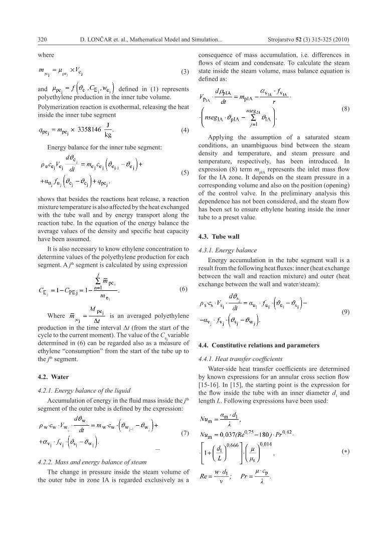
where

(3)

and defined in (1) represents polyethylene production in the inner tube volume.Polymerization reaction is exothermal, releasing the heat inside the inner tube segment

(4)

Energy balance for the inner tube segment:

(5)

shows that besides the reactions heat release, a reaction mixture temperature is also affected by the heat exchanged with the tube wall and by energy transport along the reaction tube. In the equation of the energy balance the average values of the density and specific heat capacity have been assumed.

It is also necessary to know ethylene concentration to determine values of the polyethylene production for each segment. A jth segment is calculated by using expression

(6)

Where is an averaged polyethylene

production in the time interval ∆t (from the start of the cycle to the current moment). The value of the Cej

variable determined in (6) can be regarded also as a measure of ethylene “consumption” from the start of the tube up to the jth segment.

4.2. Water

4.2.1. Energy balance of the liquidAccumulation of energy in the fluid mass inside the jth

segment of the outer tube is defined by the expression:

(7)

4.2.2. Mass and energy balance of steamThe change in pressure inside the steam volume of

the outer tube in zone IA is regarded exclusively as a

consequence of mass accumulation, i.e. differences in flows of steam and condensate. To calculate the steam state inside the steam volume, mass balance equation is defined as:

(8)

Applying the assumption of a saturated steam conditions, an unambiguous bind between the steam density and temperature, and steam pressure and temperature, respectively, has been introduced. In expression (8) term mpIA represents the inlet mass flow for the IA zone. It depends on the steam pressure in a corresponding volume and also on the position (opening) of the control valve. In the preliminary analysis this dependence has not been considered, and the steam flow has been set to ensure ethylene heating inside the inner tube to a preset value.

4.3. Tube wall

4.3.1. Energy balanceEnergy accumulation in the tube segment wall is a

result from the following heat fluxes: inner (heat exchange between the wall and reaction mixture) and outer (heat exchange between the wall and water/steam):

(9)

4.4. Constitutive relations and parameters

4.4.1. Heat transfer coefficientsWater-side heat transfer coefficients are determined

by known expressions for an annular cross section flow [15-16]. In [15], the starting point is the expression for the flow inside the tube with an inner diameter d1 and length L. Following expressions have been used:

(*)


Expressions (*) are valid for 3000 < Re < 105, 0.6 < Pr < 500, and L/d1>1, and is also used for flows in non-circular cross sections if one, instead of inner diameter, uses an equivalent diameter defined by dekv = 4A/o, where A denominates a channel cross section surface, and o the perimeter. For an annular cross section dekv = dv - du.

Having in mind the specificities of the reaction mixture flow, coefficients of the heat transfer inside the inner tube have been acquired from the equipment distributor’s documentation [17].

To speed up the simulation process, tube walls have been modelled as single-layered. The influence of the tube wall material’s heat conductivity λs =38 Wm-1K-1 and the inner tube’s wall thickness δs on the heat flux exchanged between the water and the reaction mixture through the inner tube wall has also been taken into consideration.

4.4.2. Water properties and steam conditionIn the model, constant values for water density and

specific heat capacity has been assumed (ρw = 1000 kgm-3, cw = 4182 Jkg-1K-1). Steam state in the IA zone is assumed to be saturated, making the expressions for determining the pressure, temperature and evaporation heat as follows:

pressure, bar

temperature, °C

latent heat, kJkg-1

4.4.3. Ethylene and polyethylene propertiesIn the simulations, the values for density and specific

heat capacity have been used according to [13]:ρe+pe = 530 kgm-3, c e+pe = 2427 Jkg-1K-1.

5. Simulation results

5.1. Determining the steady state

In the process of tuning parameters of the mathematical model, the focus has been put on determining the coefficients of the function describing polyethylene production (1).

For steady state calculations, model boundary conditions (inlet temperatures, mass flow rates of the water, steam and ethylene at outflow) have been acquired from available documentation. The heat transfer coefficients and properties of water and reaction mixture, calculated in advance, are also implemented in the model. By steady state calculations the necessary polymerization reaction intensity along the reactor tube is determined.

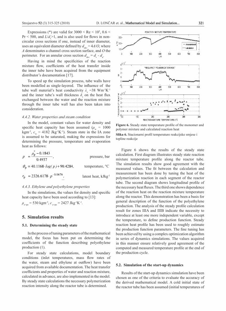
Figure 6. Steady state temperature profile of the monomer and polymer mixture and calculated reaction heatSlika 6. Stacionarni profil temperature reakcijske smjese i topline reakcije

Figure 6 shows the results of the steady state calculation. First diagram illustrates steady state reaction mixture temperature profile along the reactor tube. The simulation results show good agreement with the measured values. The fit between the calculation and measurement has been done by tuning the heat of the polymerization reaction in each segment of the reactor tube. The second diagram shows longitudinal profile of the necessary heat fluxes. The third one shows dependence of the reaction heat on the reaction mixture temperature along the reactor. This demonstration has been a basis for general description of the function of the polyethylene production. The analysis of the steady profile calculation result for zones IIIA and IIIB indicate the necessity to introduce at least one more independent variable, except the temperature, to define production function. Steady reaction heat profile has been used to roughly estimate the production function parameters. The fine tuning has been achieved by using a complex optimization algorithm in series of dynamics simulations. The values acquired in this manner ensure relatively good agreement of the computed and measured temperature profile at the end of the production cycle.

5.2. Simulation of the start-up dynamics

Results of the start-up dynamics simulation have been chosen as one of the criteria to evaluate the accuracy of the derived mathematical model. A cold initial state of the reactor tube has been assumed (initial temperatures of


water, walls and ethylene at 90 °C). Consecutive cycles of polymerization and exhaust lasting from 50 seconds have been simulated (42 seconds of polymerization phase and 8 seconds of exhaust phase with no polyethylene production occurring at this stage), as shown for initial 150 s in Figure 7. Results of the start-up process are shown in Figures 8 and 9.

Figure 7. Impulse valve relative openings during polymerization and exhaust (blow - out) cyclesSlika 7. Relativna otvorenost ventila na izlazu iz rektora u fazama polimerizacije i ispuhivanja produkata

Figure 8. Start-up of reactor, time and space profile of monomer and polymer mixture temperature Slika 8. Upuštanje - uzdužni i vremenski profil temperature reakcijske smjese

In Figures 8 and 9 one can note the slow temperature increase in the initial 500 s. In this period, the ethylene is heated by steam and water along the entire reactor length. After achieving the temperature of about 150 °C, the reaction begins, initially slow and than fast, as noticed from the steep increase of the reaction mixture temperature. At around 800 s, mixture temperature peaks in the IIB zone after which the temperature profile becomes steady. Temporal profile of the reaction mixture temperatures in the first and last segment of each zone

is shown in figure 10. Temperature oscillations of the reactant mixture, occurring after around 900 s are the result of polymerization and blow-of cycle periodically repeating with a frequency of 0.02 s-1.

Figure 9. Start-up of reactor, temperature profiles alongside reactor and in selected time instants – at the end of polymerization cycles Slika 9. Upuštanje - uzdužni profil temperature reakcijske smjese u odabranim vremenskim trenucima (na kraju ciklusa polimerizacije)

Figure 10. Start-up of reactor, temperatures of monomer and polymer mixture at inlet and outlet of the tubular reactor zonesSlika 10. Upuštanje - vremenski profil temperatura reakcijske smjese na ulazu i izlazu iz zona reaktorske cijevi


5.3. Simulation of the cycle dynamics (polymerization and blow-off)

Detailed display of temporal responses and longitudinal profiles of the characteristic process variables during one cycle (42 seconds of polymerization + 8 seconds of blow-off) in a normal operation is shown in figure 11. Comparison of simulated and measured longitudinal reaction mixture temperature profiles is presented in the upper part of figure 12. In the lower part of the figure, produced amounts of polyethylene are presented along the reactor length.

Figure 11. Normal operation, time and space profiles of monomer and polymer mixtureSlika 11. Normalni pogon - uzdužni i vremenski profil temperature reakcijske smjese

5.4. Simulation analysis of the process’ parameter sensitivity

To illustrate the capabilities of the mathematical model applicability, the influence of coolant temperature on ethylene production has been chosen as an example. During the process, a disturbance is introduced in 500th

second as a rapid water temperature decrease (from 149 °C to 120 °C) in the IIB zone inlet. Temporal and longitudinal reaction mixture and water temperatures are shown in Figures 13 and 14.

Figure 12.Temperature profiles alongside reactor at the end of polymerization cycle and mass of produced polyethyleneSlika 12.Stacionarni profil temperature reakcijske smjese i masa proizvedenog polietilena na kraju ciklusa

Figure 13. Cooling disturbance - time and space profiles of monomer and polymer mixture temperaturesSlika 13. Poremećaj hlađenja - uzdužni i vremenski profil temperature reakcijske smjese

Comparing the temperatures in the IIB zone one can note significantly slower disturbance propagation in the case of reaction mixture compared to the water temperature. Slower response to the disturbance is conditioned by inner tube wall inertia. Figure 15 shows


temporal responses of the reaction mixture temperature in the ascending and descending segments of each zone, showing that it would take around 9 cycles to achieve a new steady regime after introducing a new coolant temperature disturbance. Final illustration, as seen in Figure 16, shows that better cooling results with insignificant productivity increase.

Figure 14. Cooling disturbance - time and space profiles of steam and water temperaturesSlika 14. Poremećaj hlađenja - uzdužni i vremenski profil temperatura vode

Figure 15. Cooling disturbance - temperatures of monomer and polymer mixture at inlet and outlet of the tubular reactor zonesSlika 15. Poremećaj hlađenja - vremenski profil temperatura reakcijske smjese na ulazu i izlazu iz zona reaktorske cijevi

Figure 16. Cooling disurbacne temperature profiles alongside reactor at the end of polymerization cycle and mass of produced polyethylene, comparison of 492. s i 992. sSlika 16. Poremećaj hlađenja – stacionarni profil temperature reakcijske smjese i masa proizvedenog polietilena na kraju ciklusa, usporedba 492. s i 992. s

6. Conclusion

A mathematical model of the process dynamics of the tubular reactor for low density polyethylene polymerization has been derived. The simulation results of the characteristic operating situations show that the model provides a realistic shape of the process, with relatively small discrepancy between the calculated and available measured values for the reaction mixture temperatures.

In this work, optimization algorithms have been applied allowing fast model parameter adjustments, making it a good foundation for further improvements for a more detailed analysis of the temporal response of water and reaction mixture temperature, as well as analysis of the initiator’s influence on the polymerization process in the considered facility.

According to the level of complexity and the computational speed of the simulation, the model is suitable for inclusion into the algorithms for automatic optimization of the control system parameters, thus contributing to the quality and efficiency of process control.


REFERENCES

[1] DONG, M. K.; PIET D. I.: Modeling of branching density and branching distribution in low-density polyethylene polymerization, Chemical Engineering Science, Volume 63, Issue 8, April 2008, Pages 2035-2046.

[2] HÄFELE, M.; KIENLE, A.; BOLL, M., SCHMIDT, C.-U.: Modeling and analysis of a plant for the production of low density polyethylene, Computers & Chemical Engineering, Volume 31, Issue 2, 1 December 2006, Pages 51-65.

[3] PLADIS, P.; BALTSAS, A.; KIPARISSIDES, C.: A comprehensive investigation on high-pressure LDPE manufacturing: Dynamic modelling of compressor, reactor and separation units, Computer Aided Chemical Engineering, Volume 21, Part 1, 2006, Pages 595-600.

[4] BUDIN, R.; MIHELIĆ-BOGDANIĆ, A.; SUTLOVIĆ, I.; FILIPAN, V.: Advanced polymerization process with cogeneration and heat recovery, Applied Thermal Engineering, Volume 26, Issue 16, November 2006, Pages 1998-2004

[5] FLEŠ. D.: Polimerizacija, Tehnička enciklopedija 10, 573 – 581, LZ 1986.

[6] BRIZIĆ, M.; JANOVIĆ, Z.; ŠMIT, I.; ŠTEFANOVIĆ, D.: Polietilen, Polimerni materijali, Tehnička enciklopedija 10, 586–590, LZ 1986.

[7] WILENSKy, U.: NETLOGO Radical Polymerization model. Center for Connected Learning and Computer-Based Modeling, Northwestern University, Evanston, IL. 1998.

[8] KOLHAPURE, N.H.; FOX, R.O.: CFD analysis of micromixing effects on polymerization in tubular low-density polyethylene reactors, Chemical Engineering Science 54, pp. 3233-3242, 1999.

[9] KOLHAPURE, N.H.; FOX, R.O.: Optimizing Plant-Scale LDPE Reactors, Fluent, 2003.

[10] LORENZINI, P.; PONS, M.; VILLERMAUX, E.: Free – Radical Polymerisation Engineering – IV. Modelling Homogeneous Polymerisation of Ethylene: Determination of Model Parametres and Final Adjustment of Kinetic Coefficients, Chemical Engineering Science, Vol. 47, No. 15/16, pp. 3981-3988, 1992.KOLHAPURE, N.H.; FOX, R.O.: Optimizing Plant-Scale LDPE Reactors, Fluent, 2003.

[11] KWANG, G.K.; CHOI, K.y.: Modelling of a Multistage High – Pressure Ethylene Polymerization Reactor, Chemical Engineering Science, Vol. 49, No. 24B, pp. 4959-4969, 1994.

[12] DHIB, R.; AL-NIDWAy, N.: Modelling of free radical polymerisation of ethylene using difunctional initiators, Chemical Engineering Science 57, pp. 2735-2746, 2002.

[13] ASTEASUAIN, M.; TONELLI, S.M.; BRANDOLIN, A.; BANDONI, J.A.: Dynamic Simulation and Optimisation of Tubular Polymerisation Reactors in gPROMS, Computers and Chemical Engineering 25, pp. 509 – 515, 2001.

[14] MURATI, Kemijska kinetika, Tehička enciklopedija 7, 45 – 50, LZ 1980.

[15] KUTATELADZE, S. S.: Teploperedača i gidrodinamičeskoe soprotivlenie, Znergoatomizdat, Moskva, 1990.

[16] Inženjerski priručnik – IP1, Školska knjiga, 1996. [17] OKI LDPE Plant, plant manufacturer documentation,

ATO CHEMIE, 1981.

mathematical model and simulation of the dynamics of the

Documents