mathematical modelling in biological sciencesbhsu/biologial science.pdf · introduction in this...
TRANSCRIPT
Mathematical ModellingIn
Biological Science
Sze-Bi Hsu
Department of MathematicsTsing-Hua University, Taiwan
July 22, 2004

ii
Contents
Introduction 3
1 Continuous population model for single species 11.1 Logistic equation . . . . . . . . . . . . . . . . . . . . . . . . . . . . . 11.2 Delayed logistic equation . . . . . . . . . . . . . . . . . . . . . . . . . 21.3 Time-delay models from physiology . . . . . . . . . . . . . . . . . . . 3
2 Continuous Models for Interacting Populations 92.1 Predator-Prey models . . . . . . . . . . . . . . . . . . . . . . . . . . 92.2 Realistic Predator-Prey Model . . . . . . . . . . . . . . . . . . . . . 112.3 Competition Models . . . . . . . . . . . . . . . . . . . . . . . . . . . 20
3 Chemical Reaction Kinetics 253.1 Enzyme Kinetics . . . . . . . . . . . . . . . . . . . . . . . . . . . . . 253.2 Autocatalysis . . . . . . . . . . . . . . . . . . . . . . . . . . . . . . . 313.3 Biological Oscillators: Monotone cyclic feedback systems . . . . . . . 343.4 Biological Oscillators: Belousov-Zhabotinskii reaction . . . . . . . . 37
4 Nerve Conduction 434.1 Electrical Circuit model of the cell membrane . . . . . . . . . . . . . 43
5 Reaction diffusion equations 515.1 Simple random walk and derivation of the diffusion equation . . . . 515.2 Reaction diffusion equations . . . . . . . . . . . . . . . . . . . . . . . 535.3 Chemotaxis . . . . . . . . . . . . . . . . . . . . . . . . . . . . . . . . 53
A 57
1

2 CONTENTS
Introduction
In this lecture note we shall discuss the mathematical modelling in Biological Sci-ence. Especially we shall restrict our attentions to the following topics:
1. Continuous population models for single species, delay models in populationbiology and physiology.
2. Continuous models for inter acting populations: predator-prey model, com-petition models, mutualism or symbiosis.
3. Chemical reaction Rinetics: Michaelis-Menten theorey for enzyme-substrateRinetics.
4. Biological Oscillators: Feedback and control mechanisms, Hodgkin-Huxleytheory for nerve membrane: FitzHugh-Nagumo model.
5. Belousov-Zhabotinski Reactions.
6. Reaction Diffusion, Chemotaxis and Non-local Mechanisms.
7. Biological waves for single species model and multiple-species model.
8. Pattern formation Theory.
In each topics, we shall derive the biological models, then we do the non-dimensional analysis to reduce the model to a simple model with fewer parameters.We shall only do the elementary analysis, for example, the linearized stability anal-ysis or heuristic arguement for the models. Finally we shall show the reader thecomputation results. Basically we shall show the readers how to use the mathemat-ical software, like Matlab, Mathematica, xxp to realize the biological phenomena.The models will be nonlinear and each topics are of difficult mathematics, a chal-lenge for students to do and explore. We shall present the important references foreach topics.
3

4 CONTENTS
Scheme :
Derive Mathematical Modelsfor
Biological Phenomena
↓Nondimensional process
tosimplify the equations of the models
↓Elementary mathematical
analysis orheuristic arguements
↓Computations, theuse of mathematical
software
↓Biological Interpretations
Chapter 1
Continuous population modelfor single species
1.1 Logistic equation
The simplest population model of single species is the Malthusim model. Let N(t)be the population density of the species at time t. Assume the rate of change of thepopulation is proportional to the current population, i.e.
dN
dt= rN, N(0) = N0, r > 0 (1.1)
Then obviously N(t) = N0ert → ∞ as t → ∞. r is called the intrinsic growth
rate of the species. Model (1.1) is called the Malthusim model. It is used for thegrowth of species, like bacteria in a nutrient-unlimited supplied environment. In1848 Verhulst introduced the following logistic equation:
dN
dt= rN − bN2 (1.2)
N(0) = N0
In (1.2) the interspecific competition between the members of the species in thepopulation is considered. It can be rewritten as
dN
dt= rN
(1 − N
K
)(1.3)
N(0) = N0
Then for any N0 > 0, N(t) → K as t → ∞. K is called ”carrying capacity” of theenvironment. Although (1.3) can be solved directly by separation of variables,
N(t) =N0Kert
K + N0(ert − 1),
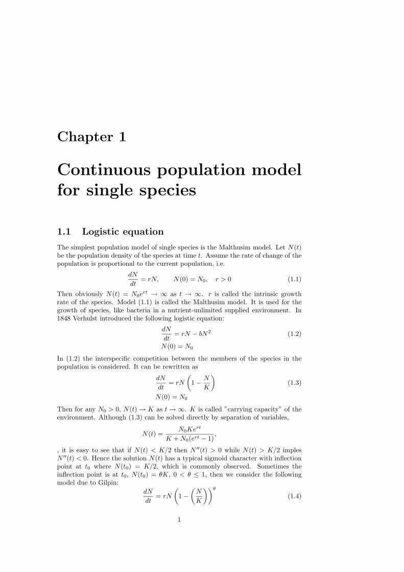
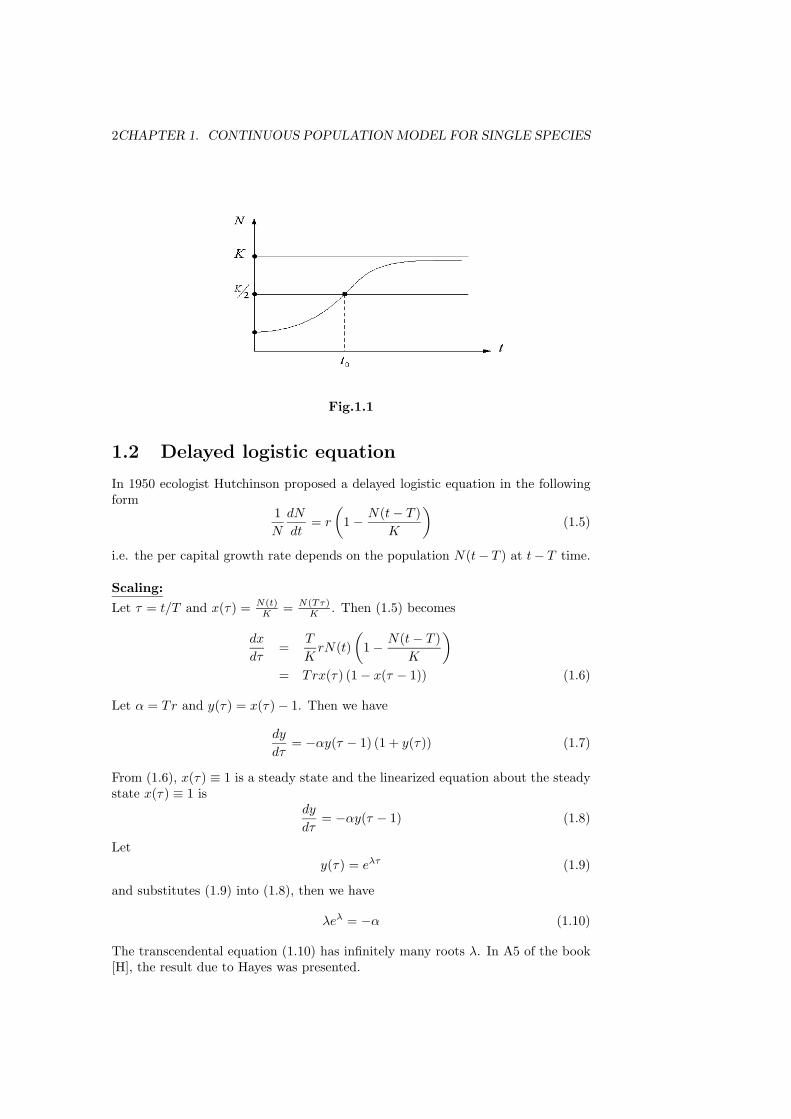
, it is easy to see that if N(t) < K/2 then N ′′(t) > 0 while N(t) > K/2 implesN ′′(t) < 0. Hence the solution N(t) has a typical sigmoid character with inflectionpoint at t0 where N(t0) = K/2, which is commonly observed. Sometimes theinflection point is at t0, N(t0) = θK, 0 < θ ≤ 1, then we consider the followingmodel due to Gilpin:
dN
dt= rN
(1 −(
N
K
))θ
(1.4)
1
2CHAPTER 1. CONTINUOUS POPULATION MODEL FOR SINGLE SPECIES
Fig.1.1
1.2 Delayed logistic equation
In 1950 ecologist Hutchinson proposed a delayed logistic equation in the followingform
1N
dN
dt= r
(1 − N(t − T )
K
)(1.5)
i.e. the per capital growth rate depends on the population N(t− T ) at t− T time.
Scaling:
Let τ = t/T and x(τ) = N(t)K = N(Tτ)
K . Then (1.5) becomes
dx
dτ=
T
KrN(t)
(1 − N(t − T )
K
)= Trx(τ) (1 − x(τ − 1)) (1.6)
Let α = Tr and y(τ) = x(τ) − 1. Then we have
dy
dτ= −αy(τ − 1) (1 + y(τ)) (1.7)
From (1.6), x(τ) ≡ 1 is a steady state and the linearized equation about the steadystate x(τ) ≡ 1 is
dy
dτ= −αy(τ − 1) (1.8)
Lety(τ) = eλτ (1.9)
and substitutes (1.9) into (1.8), then we have
λeλ = −α (1.10)
The transcendental equation (1.10) has infinitely many roots λ. In A5 of the book[H], the result due to Hayes was presented.
1.3. TIME-DELAY MODELS FROM PHYSIOLOGY 3
Theorem 1.1 All roots of the equation (z + a)ez + b = 0 where a, b ∈ R, havenegative real parts if and only if
a > −1a + b > 0b < ξ sin ξ − a cos ξ
where ξ is the root of ξ = −a tan ξ, 0 < ξ < π if a = 0 and ξ = π/2 if a = 0.
Lemma 1.3 ([H]p.255) Equation (1.7) has a Hopf bifurcation at α = π/2.For α > π/2, Jones introduced the idea of finding a cone and a map from cone
into itself, and applied a fixed point theorem of cone to prove the existence ofperiodic solutions. The reader may check the details in p.254-260 of [H].
1.3 Time-delay models from physiology
Conceptually simple feedback mechanisms are believed to be fundamental for thecontrol of a large number of different physiological processes. The simplest negativefeedback described by ordinary differential equation
dx
dt= λ − rx
In physiological situations, time lags are often important and λ and/or r are notconstants, but are some appropriate functions of x(t) and/or x(t − τ).
Delay Models in Physiology : Dynamic Diseases
Cheyne-Stokes respiration:
Cheyne-Stokes respiration is a human respiratory illness manifested by an alter-ation in the regular breathing pattern which directly related to the breath volume-the ventilation V . Let the level of arterial carbon dioxide (CO2), c(t), is monitoredby receptors which determine the level of ventilation. It is believed that these CO2-sensitive receptors are situated in the brainstem so there is an inherent time lag T ,in the overall control system for breathing levels. We assume the dependence of theventilation V on c is a Hill’s function
V = Vmaxcm(t − T )
am + cm(t − T ), m > 0.
We also assume that the removal of CO2 from the blood is proportional to theproduct of the ventilation and the level of CO2 in the blood. Let p be the constantproduction rate of CO2 in the body. Then the dynamics of the CO2 level is modelledby
dc
dt= p − bc(t) · Vmax
cm(t − T )am + cm(t − T )
x =c
a, t∗ =
pt
a, T ∗ =
pT
a, α =
abVmax
p, V ∗ =
V
Vmax
The model becomes (drop ∗)x′(t) = 1 − αx(t)V (x(t − T ))
= 1 − αx(t)xm(t − T )
1 + xm(t − T )
4CHAPTER 1. CONTINUOUS POPULATION MODEL FOR SINGLE SPECIES
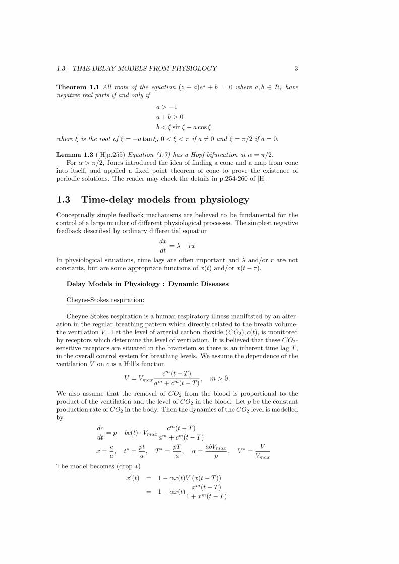
Steady state:
1 − αx0V (x0) = 0 or V (x0) = 1αx0
Linearized equation:
u = x − x0 V0 = V (x0), V ′0 =
dV
dx(x0)
u′ = −αuV0 − αx0V′0u(t − T )
Stability analysis:
u(t) = eλt ⇒ λeλt = −αeλtV0 − αx0V′0 − αx0V
′0eλ(t−T )
λ = −αV0 − αx0V′0e−λT
LetA = αV0, B = αx0V
′0
thenλ = −A − Be−λT or (λ + A) eλT + B = 0 (1.11)
Set z = λT then(
zT + A
)ez + B = 0 or (z + a) ez + b = 0, where a = AT, b = BT .
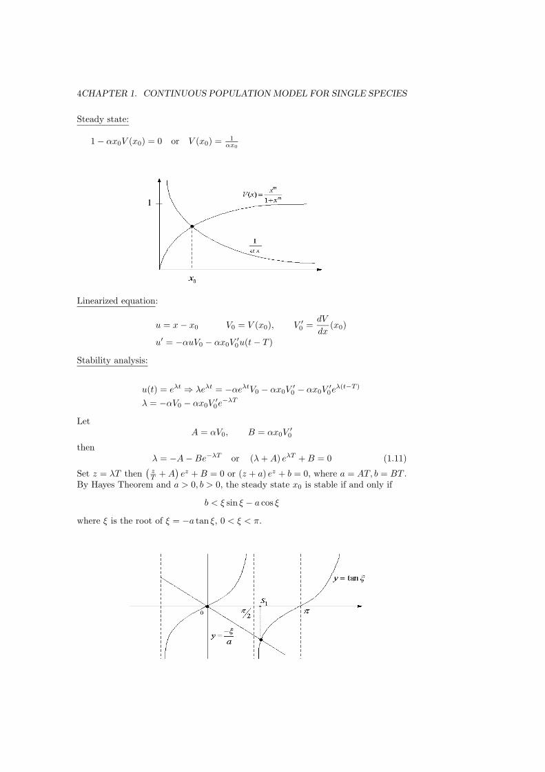
By Hayes Theorem and a > 0, b > 0, the steady state x0 is stable if and only if
b < ξ sin ξ − a cos ξ
where ξ is the root of ξ = −a tan ξ, 0 < ξ < π.
1.3. TIME-DELAY MODELS FROM PHYSIOLOGY 5
Let T be a bifurcation parameter. Set λ = µ + iω. Then (1.11) becomes
µ = −A − Be−µT cos ωT
ω = Be−µT sinωT(1.12)
We are interested in the Hopf bifurcation, i.e., the real part µ = 0. If µ = 0 then(1.12) gives, with s = ωT ,
tan s = − s
ATπ/2 < s < π.
Let µ = 0 and s = s1 then
0 = −A − B cos s1,
s1 = BT sin s1.
This implies
BT =[(AT )2 + s2
1
] 12
.
When T = 0 we have µ = −A − B < 0. Increase T from T = 0 to T satisfies
BT <[(AT )2 + s2
1
] 12
,
tan s1 = − s1AT .
(1.13)
We note that if (1.13) holds then Reλ = µ < 0 i.e. the steady state is stable. Interms of the original dimensionless variables from (1.13) the conditions are
αx0V′0T <
[(αV0T )2 + s2
1
] 12
,
tan s1 = − s1αV0T .
(1.14)
The actual parameters for normal humans have been obtained by Mackey and Glass[MG], They are
x0 = 40mmHg, p = 6mmHg/min, V0 = 7.44litre/min,
V ′0 = 4litre/minmmHg, T = 0.25min,
α = 80litre/min.
The solution of the second equation in (1.13) is s1 ≈ π/2 and
αV0T =T
x0= 0.0375.
Hence s1 αV0T and from (1.14) it follows that the inequality is approximately
V ′0 <
π
2αx0T
6CHAPTER 1. CONTINUOUS POPULATION MODEL FOR SINGLE SPECIES
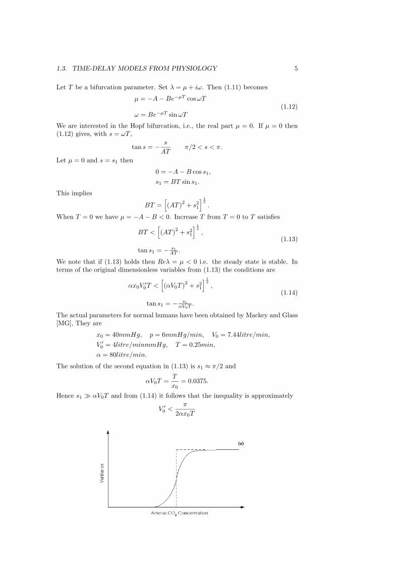
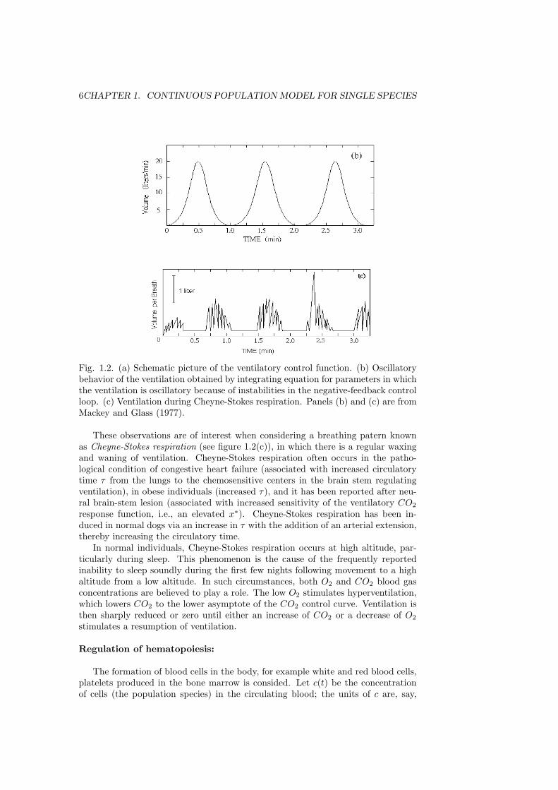
Fig. 1.2. (a) Schematic picture of the ventilatory control function. (b) Oscillatorybehavior of the ventilation obtained by integrating equation for parameters in whichthe ventilation is oscillatory because of instabilities in the negative-feedback controlloop. (c) Ventilation during Cheyne-Stokes respiration. Panels (b) and (c) are fromMackey and Glass (1977).
These observations are of interest when considering a breathing patern knownas Cheyne-Stokes respiration (see figure 1.2(c)), in which there is a regular waxingand waning of ventilation. Cheyne-Stokes respiration often occurs in the patho-logical condition of congestive heart failure (associated with increased circulatorytime τ from the lungs to the chemosensitive centers in the brain stem regulatingventilation), in obese individuals (increased τ), and it has been reported after neu-ral brain-stem lesion (associated with increased sensitivity of the ventilatory CO2
response function, i.e., an elevated x∗). Cheyne-Stokes respiration has been in-duced in normal dogs via an increase in τ with the addition of an arterial extension,thereby increasing the circulatory time.
In normal individuals, Cheyne-Stokes respiration occurs at high altitude, par-ticularly during sleep. This phenomenon is the cause of the frequently reportedinability to sleep soundly during the first few nights following movement to a highaltitude from a low altitude. In such circumstances, both O2 and CO2 blood gasconcentrations are believed to play a role. The low O2 stimulates hyperventilation,which lowers CO2 to the lower asymptote of the CO2 control curve. Ventilation isthen sharply reduced or zero until either an increase of CO2 or a decrease of O2
stimulates a resumption of ventilation.
Regulation of hematopoiesis:
The formation of blood cells in the body, for example white and red blood cells,platelets produced in the bone marrow is consided. Let c(t) be the concentrationof cells (the population species) in the circulating blood; the units of c are, say,

1.3. TIME-DELAY MODELS FROM PHYSIOLOGY 7
cells/mm3. We assume that the cells are lost at a rate proportional to their con-centration, that is like gc, which the parameter g has dimensions (day)−1. Afterthe reduction in cells in the blood stream there is about a 6 day delay before themarrow releases further cells to replenish the deficiency. We thus assume that theflux λ of cells into the blood stream depends on the cell concentration at an earliertime, namely c(t − T ), where T is the delay. Such assumptions suggest a modelequation of the form
dc(t)dt
= λ (c(t − T )) − gc(t). (1.15)
Mackey and Glass (1977) [MG] proposed two possible forms for the function (c(t − T )).The one we consider gives
dc
dt=
λamc(t − T )am + cm(t − T )
− gc, (1.16)

8CHAPTER 1. CONTINUOUS POPULATION MODEL FOR SINGLE SPECIES

Chapter 2
Continuous Models forInteracting Populations
In this chapter we shall introduce the predator-prey models, competition modelsand mutualist models.
2.1 Predator-Prey models
Let x(t) be the population density of prey, y(t) be the population density of predatorat time t. The general model for predator-prey interaction is following
dx
dt= xf(x, y)
dy
dt= yg(x, y)
x(0) > 0, y(0) > 0
where f(x, y) and g(x, y) satisfy
∂f
∂y≤ 0,
∂g
∂x≥ 0.
In 1926 Volterra first proposed a simple model for the predation of one species byanother to explain the oscillatory levels of certain fish catches in the Adriatic. Themodel is
dxdt = x (a − by)
dydt = y (cx − d)
(2.1)
The model (2.1) is known as Lotka-Volterra model since the same equations werealso derived by Lotka, a chemist, from the autocatalysis in chemical reation.
As a first step in analysing (2.1) we non-dimensionalize the system by
u(τ) =cx(t)
d, v(τ) =
by(t)a
, τ = at, α = b/a
and (2.1) becomesdudτ = u(1 − v)
u(0) > 0, v(0) > 0dvdτ = αv(u − 1)
(2.2)
9
10CHAPTER 2. CONTINUOUS MODELS FOR INTERACTING POPULATIONS
In the uv phase plane, we have
dv
du= α
v(u − 1)u(1 − v)
orv − 1
vdv + α
u − 1u
du = 0 (2.3)
Integrate (2.3) we obtain
V (u, v) =∫ v
1
ξ − 1ξ
dξ + α
∫ u
1
η − 1η
dη ≡ const (2.4)
or
v − 1 − ln v + α (u − 1 − ln u) ≡ H
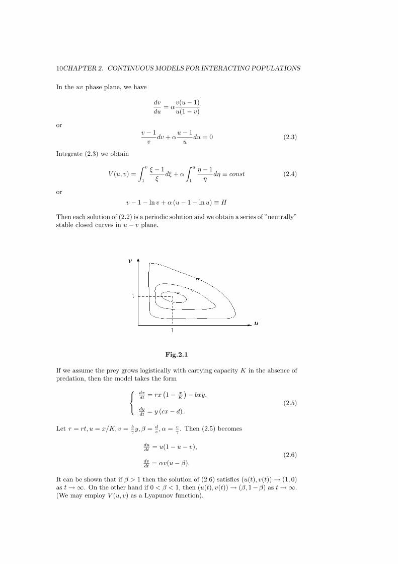
Then each solution of (2.2) is a periodic solution and we obtain a series of ”neutrally”stable closed curves in u − v plane.
Fig.2.1
If we assume the prey grows logistically with carrying capacity K in the absence ofpredation, then the model takes the form⎧⎨⎩
dxdt = rx
(1 − x
K
)− bxy,
dydt = y (cx − d) .
(2.5)
Let τ = rt, u = x/K, v = bγ y, β = d
c , α = cγ . Then (2.5) becomes
dudt = u(1 − u − v),
dvdt = αv(u − β).
(2.6)
It can be shown that if β > 1 then the solution of (2.6) satisfies (u(t), v(t)) → (1, 0)as t → ∞. On the other hand if 0 < β < 1, then (u(t), v(t)) → (β, 1−β) as t → ∞.(We may employ V (u, v) as a Lyapunov function).
2.2. REALISTIC PREDATOR-PREY MODEL 11
Fig.2.2
2.2 Realistic Predator-Prey Model
Consider the following Gause-type predator-prey system:
dxdt = xg(x) − p(x)y
dydt = (cp(x) − q(x)) y
(2.7)
where x = x(t), y = y(t) are density of prey and predator respectively. The functiong(x) satisfies
(H1) g(0) > 0, g(K) = 0 for some K > 0 and (x − K)g(x) < 0 for all x = K.For example g(x) = r
(1 − x
K
), g(x) = r
(1 − ( x
K
)θ). The functional responsep(x) satisfies
(H2) p(0) = 0, p′(x) > 0∀x ≥ 0.The death rate q(x) satisfies
(H3) q(x) > 0, q′ ≤ 0, x ≥ 0.
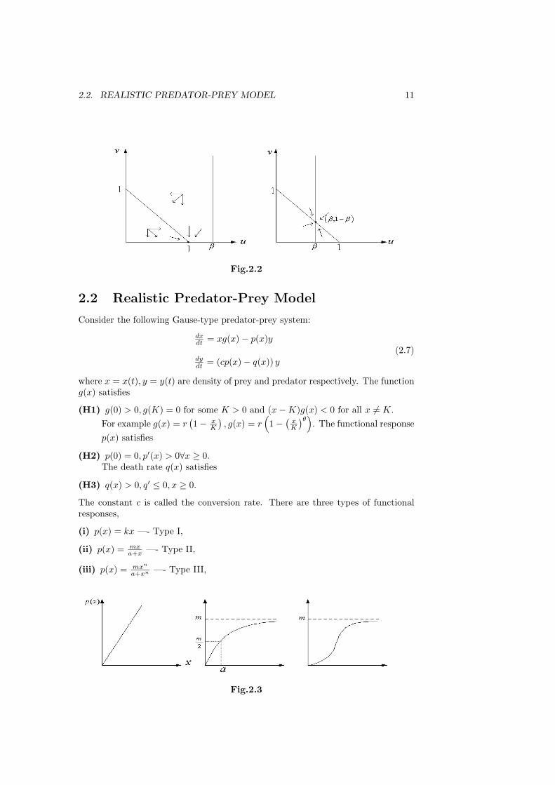
The constant c is called the conversion rate. There are three types of functionalresponses,
(i) p(x) = kx —- Type I,
(ii) p(x) = mxa+x —- Type II,
(iii) p(x) = mxn
a+xn —- Type III,
Fig.2.3

12CHAPTER 2. CONTINUOUS MODELS FOR INTERACTING POPULATIONS
Type I is the Lotka-Volterra type. Type II is called Holling’s type II functionalresponse or Michaelis-Menten type with maximal growth rate m and half saturationconstant a. Type III is also called the learning functional response since the curvep(x) is a sigmoid type curve with an inflection point.
Stability of the equilibria:There are three equilibria: (0, 0), (K, 0), (x∗, y∗).The Jacobian of the system (2.7) is
J(x, y) =[
xgx(x) + g(x) − ypx(x) ,−p(x)cypx(x) cp(x) − q(x)
].
Then
J(0, 0) =[
g(0) 00 −q(0)
]Since g(0) > 0, the equilibrium (0, 0) is a saddle point with stable manifold (x, y) :x = 0, y ≥ 0 and unstable manifold (x, y) : y = 0, x ≥ 0.
The Jacobian matrix at (K, 0) is
J(K, 0) =[
Kgx(K) ,−p(K)0 , cp(K) − q(K)
]Since gx(K) < 0, (K, 0) is stable if and only if cp(K) − q(K) < 0.
The Jacobian at interior equilibrium (x∗, y∗) is
J(x∗, y∗) =[
H(x∗) −p(x∗)y∗px(x∗) , 0
]where
H(x∗) = x∗gx(x∗) + g(x∗) − x∗g(x∗)px(x∗)p(x∗)
. (2.8)
Since the eigenvalues of J(x∗, y∗) are given by
H(x∗)2
±[H2(x∗) − 4y∗p(x∗)px(x∗)
] 12
2.
It is clear that the sign of the real parts of these eigenvalues coincide with the signof H(x∗).From this we may come to the following condusions, again utilizing y∗ = x∗g(x∗)
p(x∗) ,
H(x∗)2 − 4x∗p(x∗)px(x∗) < 0(> 0) ⇒ (x∗, y∗) is a spiral (node). (2.9)
FurtherH(x∗) < 0(> 0) ⇒ (x∗, y∗) is stable (unstable).
The prey isocline is y = xg(x)p(x) and the predator isocline is x = x∗. From (2.8)
H(x∗)x∗g(x∗)
=gx(x∗)g(x∗)
+1x∗ − px(x∗)
p(x∗)
=d
dxln[xg(x)p(x)
]|x=x∗ .
Then the stability criterion (2.9) becomes
d
dxln[xg(x)p(x)
]|x=x∗ < 0(> 0) ⇒ (x∗, y∗) is stable (unstable) (2.10)
2.2. REALISTIC PREDATOR-PREY MODEL 13
Then (2.10) is equivalent to the prey isocline
y =xg(x)p(x)
is decreasing (increasing)at x∗ ⇒ (x∗, y∗) is stable (unstable).
Example:[HHW] [C]
x′ = rx(1 − x
K
)− mxa+xy
y′ =(
mxa+x − d
)y
x(0) > 0, y(0) > 0
(2.11)
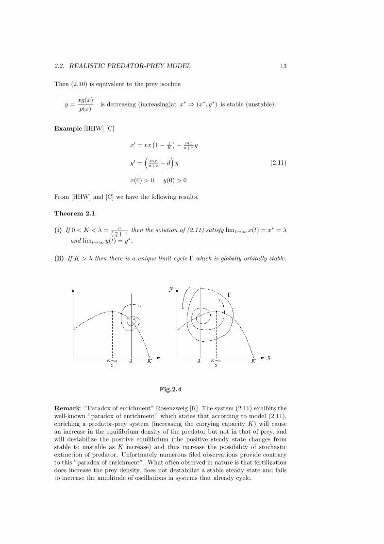
From [HHW] and [C] we have the following results.
Theorem 2.1:
(i) If 0 < K < λ = a
(md )−1
then the solution of (2.11) satisfy limt→∞ x(t) = x∗ = λ
and limt→∞ y(t) = y∗.
(ii) If K > λ then there is a unique limit cycle Γ which is globally orbitally stable.
Fig.2.4
Remark: ”Paradox of enrichment” Rosenzweig [R]. The system (2.11) exhibits thewell-known ”paradox of enrichment” which states that according to model (2.11),enriching a predator-prey system (increasing the carrying capacity K) will causean increase in the equilibrium density of the predator but not in that of prey, andwill destabilize the positive equilibrium (the positive steady state changes fromstable to unstable as K increase) and thus increase the possibility of stochasticextinction of predator. Unfortnately numerous filed observations provide contraryto this ”paradox of enrichment”. What often observed in nature is that fertilizationdoes increase the prey density, does not destabilize a stable steady state and failsto increase the amplitude of oscillations in systems that already cycle.
14CHAPTER 2. CONTINUOUS MODELS FOR INTERACTING POPULATIONS
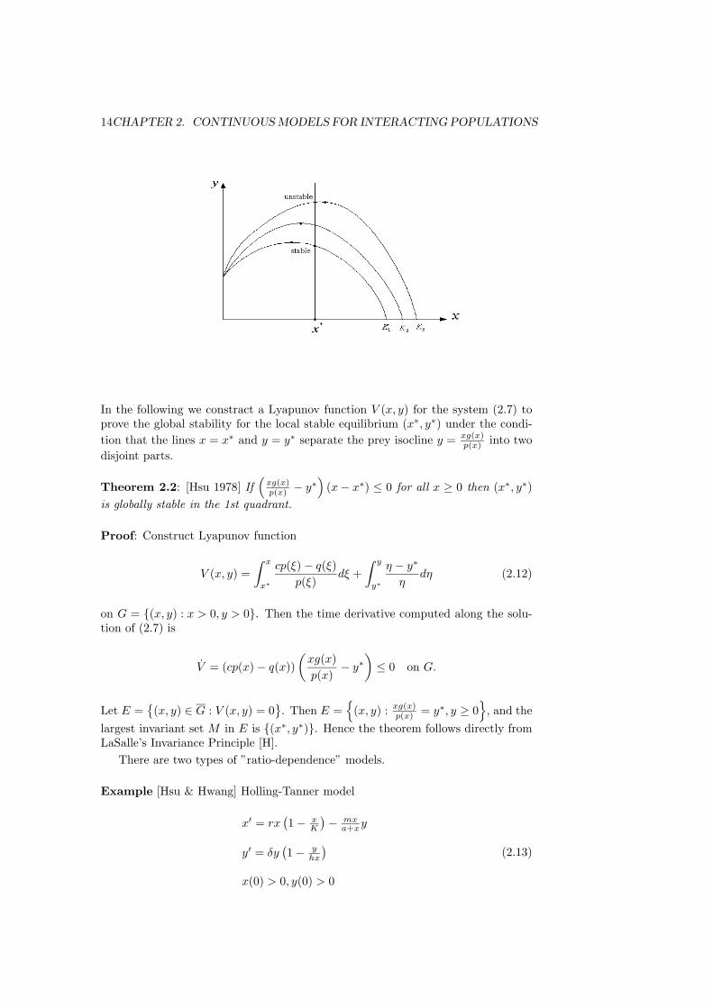
In the following we constract a Lyapunov function V (x, y) for the system (2.7) toprove the global stability for the local stable equilibrium (x∗, y∗) under the condi-tion that the lines x = x∗ and y = y∗ separate the prey isocline y = xg(x)
p(x) into twodisjoint parts.
Theorem 2.2: [Hsu 1978] If(
xg(x)p(x) − y∗
)(x − x∗) ≤ 0 for all x ≥ 0 then (x∗, y∗)
is globally stable in the 1st quadrant.
Proof: Construct Lyapunov function
V (x, y) =∫ x
x∗
cp(ξ) − q(ξ)p(ξ)
dξ +∫ y
y∗
η − y∗
ηdη (2.12)
on G = (x, y) : x > 0, y > 0. Then the time derivative computed along the solu-tion of (2.7) is
V = (cp(x) − q(x))(
xg(x)p(x)
− y∗)
≤ 0 on G.
Let E =(x, y) ∈ G : V (x, y) = 0
. Then E =
(x, y) : xg(x)
p(x) = y∗, y ≥ 0
, and thelargest invariant set M in E is (x∗, y∗). Hence the theorem follows directly fromLaSalle’s Invariance Principle [H].
There are two types of ”ratio-dependence” models.
Example [Hsu & Hwang] Holling-Tanner model
x′ = rx(1 − x
K
)− mxa+xy
y′ = δy(1 − y
hx
)x(0) > 0, y(0) > 0
(2.13)
2.2. REALISTIC PREDATOR-PREY MODEL 15
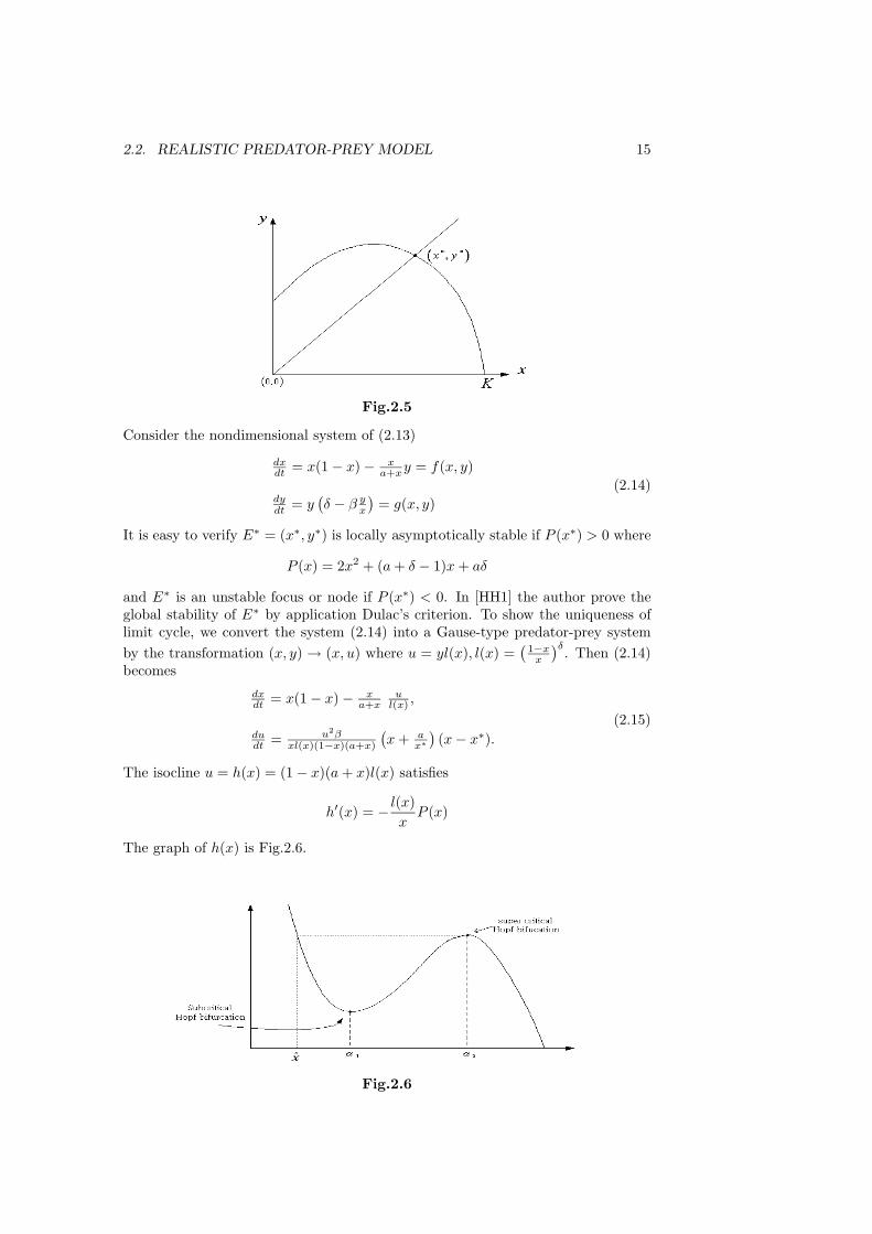
Fig.2.5
Consider the nondimensional system of (2.13)
dxdt = x(1 − x) − x
a+xy = f(x, y)
dydt = y
(δ − β y
x
)= g(x, y)
(2.14)
It is easy to verify E∗ = (x∗, y∗) is locally asymptotically stable if P (x∗) > 0 where
P (x) = 2x2 + (a + δ − 1)x + aδ
and E∗ is an unstable focus or node if P (x∗) < 0. In [HH1] the author prove theglobal stability of E∗ by application Dulac’s criterion. To show the uniqueness oflimit cycle, we convert the system (2.14) into a Gause-type predator-prey systemby the transformation (x, y) → (x, u) where u = yl(x), l(x) =
(1−x
x
)δ. Then (2.14)becomes
dxdt = x(1 − x) − x
a+xu
l(x) ,
dudt = u2β
xl(x)(1−x)(a+x)
(x + a
x∗)(x − x∗).
(2.15)
The isocline u = h(x) = (1 − x)(a + x)l(x) satisfies
h′(x) = − l(x)x
P (x)
The graph of h(x) is Fig.2.6.
Fig.2.6

16CHAPTER 2. CONTINUOUS MODELS FOR INTERACTING POPULATIONS
If x∗ < x then we construct a Lyapunov function like (2.12) to show that (x∗, y∗)is global stable. For α1 < x∗ < α2, (x∗, y∗) is unstable and by Poincare-BendixsonTheorem there exists a limit cycle. The problem of uniqueness of limit cycle wasstudied in [HH2].
For x∗ > α2, E∗ is global stable. For x < x∗ < α1, there may exists limit cycleseven E∗ is stable due to the subcritical Hopf bifurcation.
Example: [HHK]
x′ = rx(1 − x
K
)− c( xy )
a+( xy )y = rx
(1 − x
K
)− cxyay+x = F1(x, y)
y′ =[
m( xy )
a+( xy ) − d
]y =(
mxay+x − d
)y = F2(x, y)
(2.16)
This model demostrates the possibilities of simultaneous extinction of predator andprey and the outcomes depending on the initial populations.
We note that (0, 0) is also an equilibrium of (2.16) for
lim(x,y)→(0,0)
F1(x, y) = lim(x,y)→(0,0)
F2(x, y) = 0
With the scalingt → rt, x → x/K, y → my
K,
(2.16) is converted into
x′(t) = x(1 − x) − sxyx+y
y′(t) = δy(−r + xx+y )
(2.17)
where s = cma , δ = f
a , df .
Consider the change of variables (x, y) → (u, y), u = xy , then (2.17) is reduced
to the following Gause-type predator-prey system
u′(t) = g(u) − ϕ(u)y
y′(t) = ψ(u)y(2.18)
where
g(u) = u(A + Bu)/(1 + u),ϕ(u) = u2,
ψ(u) = δ
(u
u + 1− r
)A = 1 + δr − s, B = 1 + δr − δ.
(2.18) can also be rewritten as
u′(t) = ϕ(u) (h(u) − y)
y′(t) = ψ(u)y(2.19)
we see that the prey isocline of (2.18) is given by
y =g(u)ϕ(u)
= h(u) =A + Bu
u(u + 1).

2.2. REALISTIC PREDATOR-PREY MODEL 17
There are several cases for the shapes of prey-isoclines for different A and B. (SeeFig. 2.7)
Fig.2.7: Scenarios of the shape of y = h(u).
The direction field for (2.19) under various conditions is shown as in Fig. 2.8.
18CHAPTER 2. CONTINUOUS MODELS FOR INTERACTING POPULATIONS
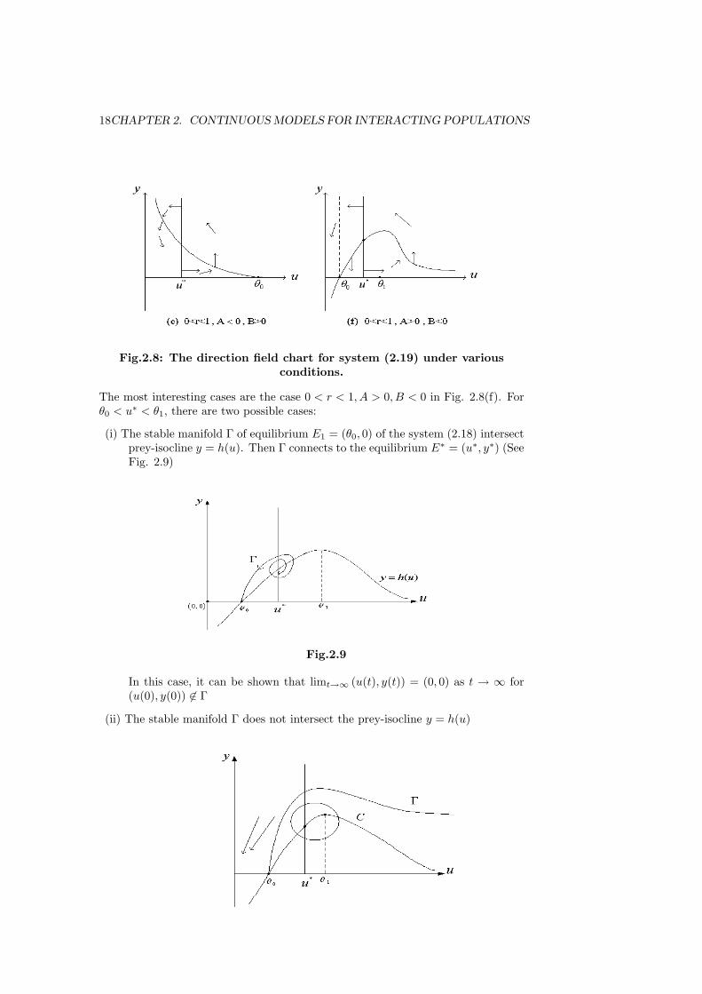
Fig.2.8: The direction field chart for system (2.19) under variousconditions.
The most interesting cases are the case 0 < r < 1, A > 0, B < 0 in Fig. 2.8(f). Forθ0 < u∗ < θ1, there are two possible cases:
(i) The stable manifold Γ of equilibrium E1 = (θ0, 0) of the system (2.18) intersectprey-isocline y = h(u). Then Γ connects to the equilibrium E∗ = (u∗, y∗) (SeeFig. 2.9)
Fig.2.9
In this case, it can be shown that limt→∞ (u(t), y(t)) = (0, 0) as t → ∞ for(u(0), y(0)) ∈ Γ
(ii) The stable manifold Γ does not intersect the prey-isocline y = h(u)
2.2. REALISTIC PREDATOR-PREY MODEL 19
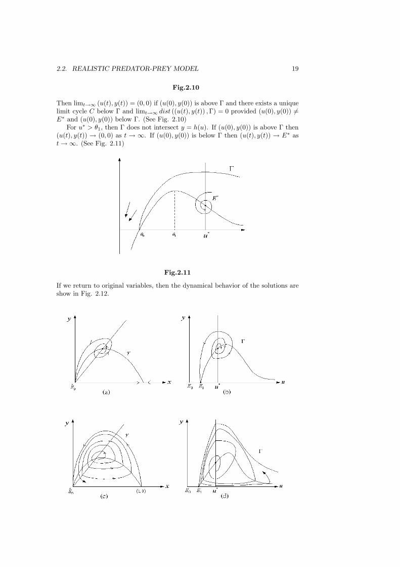
Fig.2.10
Then limt→∞ (u(t), y(t)) = (0, 0) if (u(0), y(0)) is above Γ and there exists a uniquelimit cycle C below Γ and limt→∞ dist ((u(t), y(t)) ,Γ) = 0 provided (u(0), y(0)) =E∗ and (u(0), y(0)) below Γ. (See Fig. 2.10)
For u∗ > θ1, then Γ does not intersect y = h(u). If (u(0), y(0)) is above Γ then(u(t), y(t)) → (0, 0) as t → ∞. If (u(0), y(0)) is below Γ then (u(t), y(t)) → E∗ ast → ∞. (See Fig. 2.11)
Fig.2.11
If we return to original variables, then the dynamical behavior of the solutions areshow in Fig. 2.12.
20CHAPTER 2. CONTINUOUS MODELS FOR INTERACTING POPULATIONS
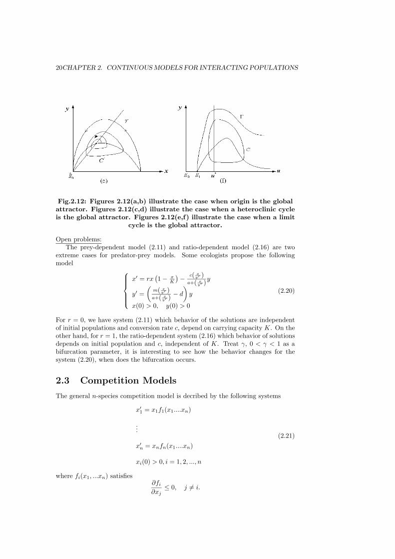
Fig.2.12: Figures 2.12(a,b) illustrate the case when origin is the globalattractor. Figures 2.12(c,d) illustrate the case when a heteroclinic cycleis the global attractor. Figures 2.12(e,f) illustrate the case when a limit
cycle is the global attractor.
Open problems:The prey-dependent model (2.11) and ratio-dependent model (2.16) are two
extreme cases for predator-prey models. Some ecologists propose the followingmodel ⎧⎪⎪⎪⎨⎪⎪⎪⎩
x′ = rx(1 − x
K
)− c( xyr )
a+( xyr )y
y′ =(
m( xyr )
a+( xyr ) − d
)y
x(0) > 0, y(0) > 0
(2.20)
For r = 0, we have system (2.11) which behavior of the solutions are independentof initial populations and conversion rate c, depend on carrying capacity K. On theother hand, for r = 1, the ratio-dependent system (2.16) which behavior of solutionsdepends on initial population and c, independent of K. Treat γ, 0 < γ < 1 as abifurcation parameter, it is interesting to see how the behavior changes for thesystem (2.20), when does the bifurcation occurs.
2.3 Competition Models
The general n-species competition model is decribed by the following systems
x′1 = x1f1(x1....xn)
...
x′n = xnfn(x1....xn)
xi(0) > 0, i = 1, 2, ..., n
(2.21)
where fi(x1, ...xn) satisfies∂fi
∂xj≤ 0, j = i.
2.3. COMPETITION MODELS 21
In this section we first consider two-species competition model
x′1 = x1f1(x1, x2) ∂f1
∂x2≤ 0, ∂f2
∂x1≤ 0
x′2 = x2f2(x1, x2)
(2.22)
Lotka-Volterra two-species competition model:
dx1dt = r1x1
(1 − x1
f1
)− α1x1x2
dx2dt = r2x2
(1 − x2
K2
)− α2x1x2
(2.23)
There are equilibria: E0 = (0, 0), E1 = (K1, 0) and E2 = (0,K2). The interior equi-librium at E∗ = (x∗
1, x∗2) exists under following case (iii) and (iv). The varational
matrix E(x1, x2) is
A(x1, x2) =
⎡⎣ γ1
(1 − x1
K1
)− α1x2 − γ1
K1x1, −α1x1
−α2x2, γ2
(1 − x2
K2
)− α2x1 − γ2
K2x2
⎤⎦At E0,
A(0, 0) =[
γ1 00 γ2
]E0 is a source or a repeller.At E1 = (K, 0)
A(K1, 0) =[ −γ1, −α1K1
0, γ2 − α2K1
]At E2 = (0,K2)
A(0,K2) =[
γ1 − α1K2, 0−α2K2, 0
]There are four cases according to the position of isoclines L1 : γ1
(1 − x1
K1
)−α1x2 =
0 and L2 : γ2
(1 − x2
K2
)− α2x1 = 0:
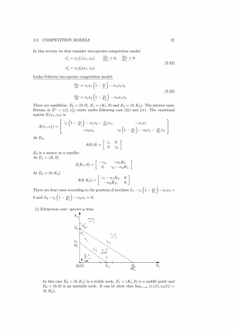
(i) Extinction case: species y wins
In this case E2 = (0,K2) is a stable node, E1 = (K1, 0) is a saddle point andE0 = (0, 0) is an unstable node. It can be show that limt→∞ (x1(t), x2(t)) =(0,K2).

22CHAPTER 2. CONTINUOUS MODELS FOR INTERACTING POPULATIONS
(ii) Extinction case: species x1 win.
In this case E1 = (K1, 0) is a stable node, E2 = (0,K2) is a saddle pointand E0 = (0, 0) is an unstable node. It can be shown limt→∞ (x1(t), x2(t)) =(K1, 0).
(iii) Coexistence case:
In this case E1 = (K1, 0) and E2 = (0,K2) are saddle point, E0 = (0, 0) is anunstable node. It can be shown limt→∞ (x1(t), x2(t)) = (x∗
1, x∗2).
The variational matrix for E∗ is
A(x∗1, x
∗2) =[ − γ1
K1x∗
1, −α1x∗1
−α2x∗2, − γ2
K2x∗
2
]The characteristic polynomial of A(x∗, y∗) is
λ2 +(
γ1
K1x∗ +
γ2
K2x∗
2
)λ + x∗
1x∗2
(γ1γ2
K1K2− α1α2
)= 0
Since γ2α2
> K1, γ1α1
> K2, it follows that E∗ = (x∗1, x
∗2) is a stable node.
2.3. COMPETITION MODELS 23
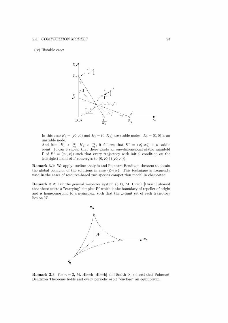
(iv) Bistable case:
In this case E1 = (K1, 0) and E2 = (0,K2) are stable nodes. E0 = (0, 0) is anunstable node.And from E1 > γ2
α2, K2 > γ1
α1, it follows that E∗ = (x∗
1, x∗2) is a saddle
point. It can e shown that there exists an one-dimensional stable manifoldΓ of E∗ = (x∗
1, x∗2) such that every trajectory with initial condition on the
left(right) hand of Γ converges to (0,K2) ((K1, 0)).
Remark 3.1: We apply isocline analysis and Poincare-Bendixon theorem to obtainthe global behavior of the solutions in case (i)–(iv). This technique is frequentlyused in the cases of resource-based two species competition model in chemostat.
Remark 3.2: For the general n-species system (3.1), M. Hirsch [Hirsch] showedthat there exists a ”carrying” simplex W which is the boundary of repeller of originand is homeomorphic to a n-simplex, such that the ω-limit set of each trajectorylies on W .
Remark 3.3: For n = 3, M. Hirsch [Hirsch] and Smith [S] showed that Poincare-Bendixon Theorems holds and every periodic orbit ”enclose” an equilibrium.
24CHAPTER 2. CONTINUOUS MODELS FOR INTERACTING POPULATIONS
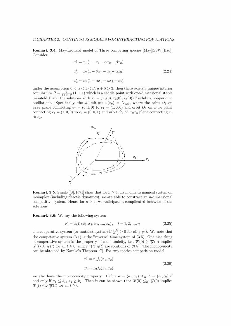
Remark 3.4: May-Leonard model of Three competing species [May][SSW][Hsu].Consider
x′1 = x1 (1 − x1 − αx2 − βx3)
x′2 = x2 (1 − βx1 − x2 − αx3)
x′3 = x3 (1 − αx1 − βx2 − x3)
(2.24)
under the assumption 0 < α < 1 < β, α +β > 2, then there exists a unique interiorequilibrium P = 1
1+α+β (1, 1, 1) which is a saddle point with one-dimensional stablemanifold Γ and the solutions with x0 = (x1(0), x2(0), x3(0)) Γ exhibits nonperiodicoscillations. Specifically, the ω-limit set ω(x0) = O123, where the orbit O3 onx1x2 plane connecting e2 = (0, 1, 0) to e1 = (1, 0, 0) and orbit O2 on x1x3 planeconnecting e1 = (1, 0, 0) to e3 = (0, 0, 1) and orbit O1 on x2x3 plane connecting e3
to e2.
Remark 3.5: Smale [[S], P.71] show that for n ≥ 4, given only dynamical system onn-simplex (including chaotic dynamics), we are able to constract an n-dimensionalcompetitive system. Hence for n ≥ 4, we anticipate a complicated behavior of thesolutions.
Remark 3.6: We say the following system
x′i = xifi (x1, x2, x3, ...., xn) , i = 1, 2, ...., n (2.25)
is a cooperative system (or mutalist system) if ∂fi
∂xj≥ 0 for all j = i. We note that
the competitive system (3.1) is the ”reverse” time system of (3.5). One nice thingof cooperative system is the property of monotonicity, i.e., −→x (0) ≥ −→y (0) implies−→x (t) ≥ −→y (t) for all t ≥ 0, where x(t), y(t) are solutions of (3.5). The monotonicitycan be obtained by Kamke’s Theorem [C]. For two species competition model
x′1 = x1f1(x1, x2)
x′2 = x2f2(x1, x2)
(2.26)
we also have the monotonicity property. Define a = (a1, a2) ≤K b = (b1, b2) ifand only if a1 ≤ b1, a2 ≥ b2. Then it can be shown that −→x (0) ≤K
−→y (0) implies−→x (t) ≤K
−→y (t) for all t ≥ 0.
Chapter 3
Chemical Reaction Kinetics
3.1 Enzyme Kinetics
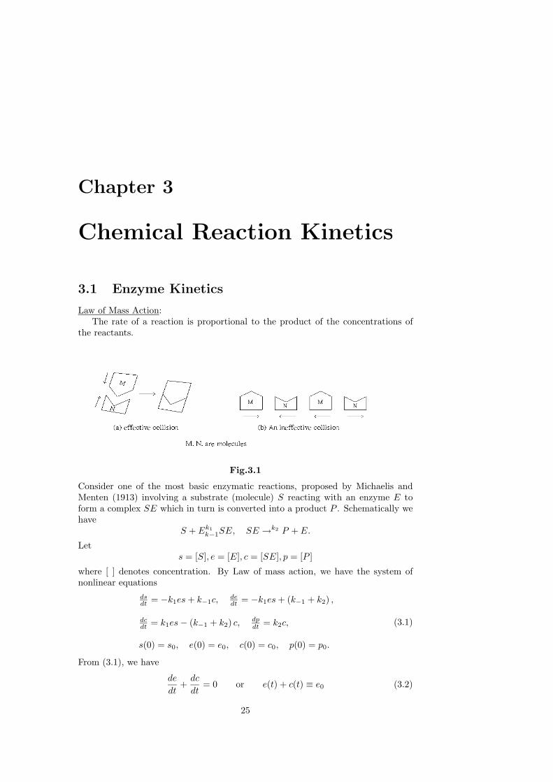
Law of Mass Action:The rate of a reaction is proportional to the product of the concentrations of
the reactants.
Fig.3.1
Consider one of the most basic enzymatic reactions, proposed by Michaelis andMenten (1913) involving a substrate (molecule) S reacting with an enzyme E toform a complex SE which in turn is converted into a product P . Schematically wehave
S + Ek1k−1SE, SE →k2 P + E.
Lets = [S], e = [E], c = [SE], p = [P ]
where [ ] denotes concentration. By Law of mass action, we have the system ofnonlinear equations
dsdt = −k1es + k−1c,
dedt = −k1es + (k−1 + k2) ,
dcdt = k1es − (k−1 + k2) c, dp
dt = k2c,
s(0) = s0, e(0) = e0, c(0) = c0, p(0) = p0.
(3.1)
From (3.1), we have
de
dt+
dc
dt= 0 or e(t) + c(t) ≡ e0 (3.2)
25
26 CHAPTER 3. CHEMICAL REACTION KINETICS
By (3.2) we have
dsdt = −k1e0s + (k1s + k−1) c,
dcdt = k1e0s − (k1s + k−1 + k2) c,
s(0) = s0, c(0) = 0
(3.3)
With the nondimensionalization
τ = k1e0t, u(τ) = s(t)s0
, v(τ) = c(t)e0
λ = k2k1s0
, K = k−1+k2k1s0
, ε = e0s0
(3.4)
the system (3.3) become
dudτ = −u + (u + K − λ) v
ε dvdτ = u − (u + K) v
u(0) = 1, v(0) = 0
(3.5)
where 0 < ε 1 and from (3.4), K > λ.
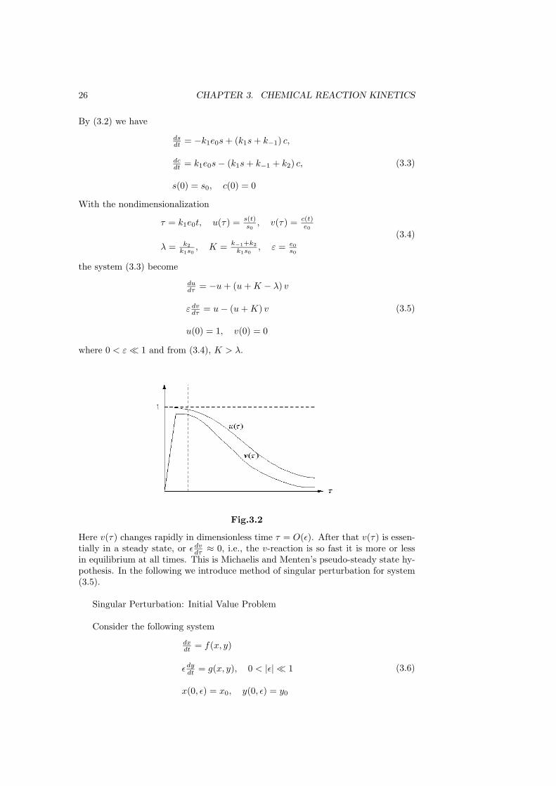
Fig.3.2
Here v(τ) changes rapidly in dimensionless time τ = O(ε). After that v(τ) is essen-tially in a steady state, or ε dv
dτ ≈ 0, i.e., the v-reaction is so fast it is more or lessin equilibrium at all times. This is Michaelis and Menten’s pseudo-steady state hy-pothesis. In the following we introduce method of singular perturbation for system(3.5).
Singular Perturbation: Initial Value Problem
Consider the following system
dxdt = f(x, y)
εdydt = g(x, y), 0 < |ε| 1
x(0, ε) = x0, y(0, ε) = y0
(3.6)
3.1. ENZYME KINETICS 27
If we set ε = 0 in (3.6), then
dxdt = f(x, y), x(0) = x0
0 = g(x, y)(3.7)
Assume g(x, y) = 0 can be solved as
y = ϕ(x) (3.8)
Substitute (3.8) into (3.7), then we have
dxdt = f (x, ϕ(x))
x(0) = x0
(3.9)
Let X0(t), 0 ≤ t ≤ 1 be the unique solution of (3.9) and Y0(t) = ϕ (X0(t)). Ingeneral Y0(0) = y. Assume the following hypothesis:
There exists K > 0 such that for 0 ≤ t ≤ 1
[∂g
∂y
] ∣∣∣∣∣∣∣ x = X0(t)y = Y0(t)
≤ −K(H)and
[∂g
∂y
] ∣∣∣∣∣∣∣ x = X0(t)y = λ
≤ −Kforall
λ lying between Y (0) and y0. We shall prove that
limε↓0
x(t, ε) = X0(t), limε↓0
y(t, ε) = Y0(t)
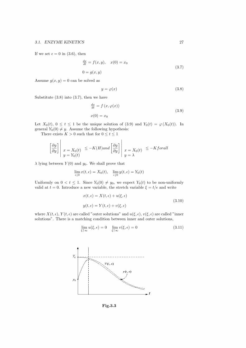
Uniformly on 0 < t ≤ 1. Since Y0(0) = y0, we expect Y0(t) to be non-uniformlyvalid at t = 0. Introduce a new variable, the stretch variable ξ = t/ε and write
x(t, ε) = X(t, ε) + u(ξ, ε)
y(t, ε) = Y (t, ε) + v(ξ, ε)(3.10)
where X(t, ε), Y (t, ε) are called ”outer solutions” and u(ξ, ε), v(ξ, ε) are called ”innersolutions”. There is a matching condition between inner and outer solutions,
limξ↑∞
u(ξ, ε) = 0 limξ↑∞
v(ξ, ε) = 0 (3.11)
Fig.3.3

28 CHAPTER 3. CHEMICAL REACTION KINETICS
Step 1: Finding outer solutions X(t, ε) and Y (t, ε).Let
X(t, ε) =∞∑
n=0
εnXn(t), Y (t, ε) =∞∑
n=0
εnYn(t). (3.12)
Do the regular perturbation for system (3.6), i.e. substitute (3.12) into (3.6) andcompare εn-term for n = 0, 1, 2, ..... Compute
f (X(t, ε), Y (t, ε)) = f (∑
εnXn,∑
εnYn)
= f (X0, Y0) + ε
[(∂f∂x
)X0,Y0
X1 +(
∂f∂y
)X0,Y0
Y1
]+ O(ε2),
g (X(t, ε), Y (t, ε)) = g (∑
εnXn,∑
εnYn)
= g (X0, Y0) + ε
[(∂g∂x
)X0,Y0
X1 +(
∂g∂y
)X0,Y0
Y1
]+ O(ε2)
(3.13)
The comparison of ε2 term by substituting (3.11) into (3.6) yields
O(1)
dX0dt = f(X0, Y0)
= g(X0, Y0)(3.14)
O(ε)
dX1dt =(
∂f∂x
)X0,Y0
X1 +(
∂f∂y
)X0,Y0
Y1
0 =(
∂g∂x
)X0,Y0
X1 +(
∂g∂y
)X0,Y0
Y1 − dY0dt
(3.15)
In (3.14) X0(t), Y0(t) satisfy
Y0(t) = ϕ (X0(t)) ,
dX0dt = f (X0, ϕ(X0)) ,
X0(0) = x0.
(3.16)
From (3.15), we obtain
Y1(t) =
[dY0
dt−(
∂g
∂x
)X0,Y0
X1
]/(∂g
∂y
)X0,Y0
, (3.17)
and X1(t) satisfies
dX1dt = ψ1(t)X1 + µ1(t)
X1(0) = 0(3.18)
3.1. ENZYME KINETICS 29
where
ψ1(t) =(
∂f
∂x
)X0,Y0
−(
∂f∂y
)(∂g∂x
)(
∂g∂y
) |X0,Y0 ,
µ1(t) =
(∂g∂y
)X0,Y0
dY0dt(
∂g∂y
)X0,Y0
·
Inductively we shall have for i = 2, 3, .....
Yi(t) = αi(t) + βi(t)Xi(t)
dXi
dt = ψi(t)Xi + µi(t),
Xi(0) = 0.
(3.19)
for x(0, ε) = X(0, ε) = x0 =∑∞
i=1 Xi(0)εn it follows that X0(0) = x0 and Xi(0) = 0for i = 1, 2, .....
Step 2: Inner expansion at sigular layer near t = 0.From (3.6) and (3.10), ξ = t/ε, we have
dudξ = d
dξ (x(εξ, ε) − X(εξ, ε))
= εf (X(ξε, ε) + u(ξ, ε), Y (ξε, ε) + v(ξ, ε))
−εf (X(ξε, ε), Y (ξε, ε))
dvdξ = g (X(ξε, ε) + u(ξ, ε), Y (ξε, ε) + v(ξ, ε))
−g (X(ξε, ε), Y (ξε, ε))
u(0, ε) = x(0, ε) − X(0, ε) = 0
v(0, ε) = y0 − Y (0, ε) = 0
(3.20)
Let
u(ξ, ε) =∞∑
n=0
un(ξ)εn, v(ξ, ε) =∞∑
n=0
vn(ξ)εn. (3.21)
Expand (3.20) in power series in ε by (3.21) and compare the coefficients on bothsides of (3.20), we have set ε = 0, we obtain
O(1) ⎧⎨⎩du0dξ = 0
⇒ u0(ξ) ≡ 0u0(0) = 0
(3.22)
30 CHAPTER 3. CHEMICAL REACTION KINETICS
and ⎧⎪⎪⎪⎪⎨⎪⎪⎪⎪⎩
dV0dξ = g (X0(0), Y0(0) + V0(ξ)) − g (X0(0), Y0(0))
≡M.V.T V0(ξ)G (V0(ξ))
V0(0) = y0 − Y0(0) (Boundary layer jump)
(3.23)
From hypothesis (H), G (V0(ξ)) ≤ −K < 0, |V0(ξ)| initially decreases and |V0(ξ)| ≤|V0(0)|e−Kξ for ξ > 0 small.
O(1): ⎧⎪⎪⎪⎪⎨⎪⎪⎪⎪⎩
du1dξ = f [X0(0), Y0(0) + V0(ξ)] − f (X0(0), Y0(0))
≡ V0(ξ)F (V0(ξ))
u1(0) = 0
(3.24)
Once V0(ξ) is solved by (3.23), we solve (3.24) and obtain
u1(ξ) =∫ ξ
∞v0(s)F (v0(s)) ds
by the matching condition (3.11) u1(∞) = 0.Hence
x(t, ε) ∼ X0(t) + ε [X1(t) + u1 (t/ε)] + O(ε)2
y(t, ε) ∼ Y0(t) + v0 (t/ε) + O(ε)
Now we go back to the Michaelis-Menten Kinetics
dxdt = f(x, y) = −x + (x + K − λ) y, K > 0, λ > 0
εdydt = g(x, y) = x − (x + K) y
(3.25)
Let
x(t, ε) = X(t, ε) + u(ξ, ε) =∞∑
n=0
εnXn(t) +∞∑
n=0
εnun(t)
y(t, ε) = Y (t, ε) + v(ξ, ε) =∞∑
n=0
εnYn(t) +∞∑
n=0
εnvn(t)
Then from (3.16)
Y0(t) = ϕ (X0(t)) =X0(t)
X0(t) + K(3.26)
where X0(t) satisfies⎧⎨⎩dxdt = −x + (x + K − λ) x
x+K = −λxx+K
x(0) = x0 = 1
Then X0(t) satisfiesX0(t) + K ln X0(t) = 1 − λt (3.27)
3.2. AUTOCATALYSIS 31
From (3.23) we obtain
dV0
dξ= [x0 − (x0 + K) (Y0(0) + v0(ξ))] − [x0 − (x0 + K) Y0(0)]
= − (x0 + K) v0(ξ)v0(0) = y0 − Y0(0), x0 = 1, y0 = 0
and
v0(ξ) =(
y0 − x0
x0 + K
)e−(x0+K)ξ
=( −1
1 + K
)e−(1+K)ξ
Hence
y(t, ε) ∼ x0(t)x0(t) + K
+( −1
1 + K
)e−(1+K)ξ(t/ε).
From (3.24)
du1
dξ= f (x0(0), Y0(0) + V0(ξ)) − f (X0(0), Y0(0))
= (1 + K − λ) v0(ξ) =λ − (1 + K)
1 + Ke−(1+K)ξ
u1(∞) = 0,u1(ξ) = ((1 + K) − λ) e−(1+K)ξ
3.2 Autocatalysis
Autocatalysis is the process where by a chemical is involved in its own production.
Example: A + Xk1−→←−−
k−1
2X
Suppose A is maintained at constant concentration, by the law of mass actionwe have
dx
dt= k1ax − k−1x
2 (3.28)
where x = [X], a ≡ [A]. The autocatalysis reaction exhibits a strong feedback withthe ”product” inhibiting the reaction rate.
Example: A + Xk1−→←−−
k−1
2X,B + X →k2 C. X is used up in the production of C.
dxdt = k1ax − k−1x
2 − k2bx
= (k1a − k2b) x − k−1x2
(3.29)
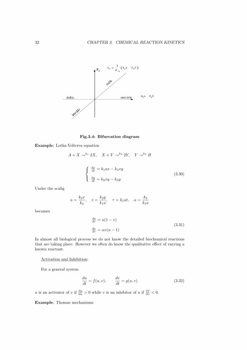
32 CHAPTER 3. CHEMICAL REACTION KINETICS
Fig.3.4: Bifurcation diagram
Example: Lotka-Volterra equation
A + X →k1 2X, X + Y →k2 2Y, Y →k3 B
⎧⎨⎩dxdt = k1ax − k2xy
dydt = k2xy − k3y
(3.30)
Under the scalig
u =k2x
k3, v =
k2y
k1a, τ = k1at, α =
k3
k1a
becomes
dudτ = u(1 − v)
dvdτ = αv(u − 1)
(3.31)
In almost all biological process we do not know the detailed biochemical reactionsthat are taking place. However we often do know the qualitative effect of varying aknown reactant.
Activation and Inhibition:
For a general system
du
dt= f(u, v),
dv
dt= g(u, v) (3.32)
u is an activator of v if ∂g∂u > 0 while v is an inhibitor of u if ∂f
∂v < 0.
Example: Thomas mechanisms
3.2. AUTOCATALYSIS 33
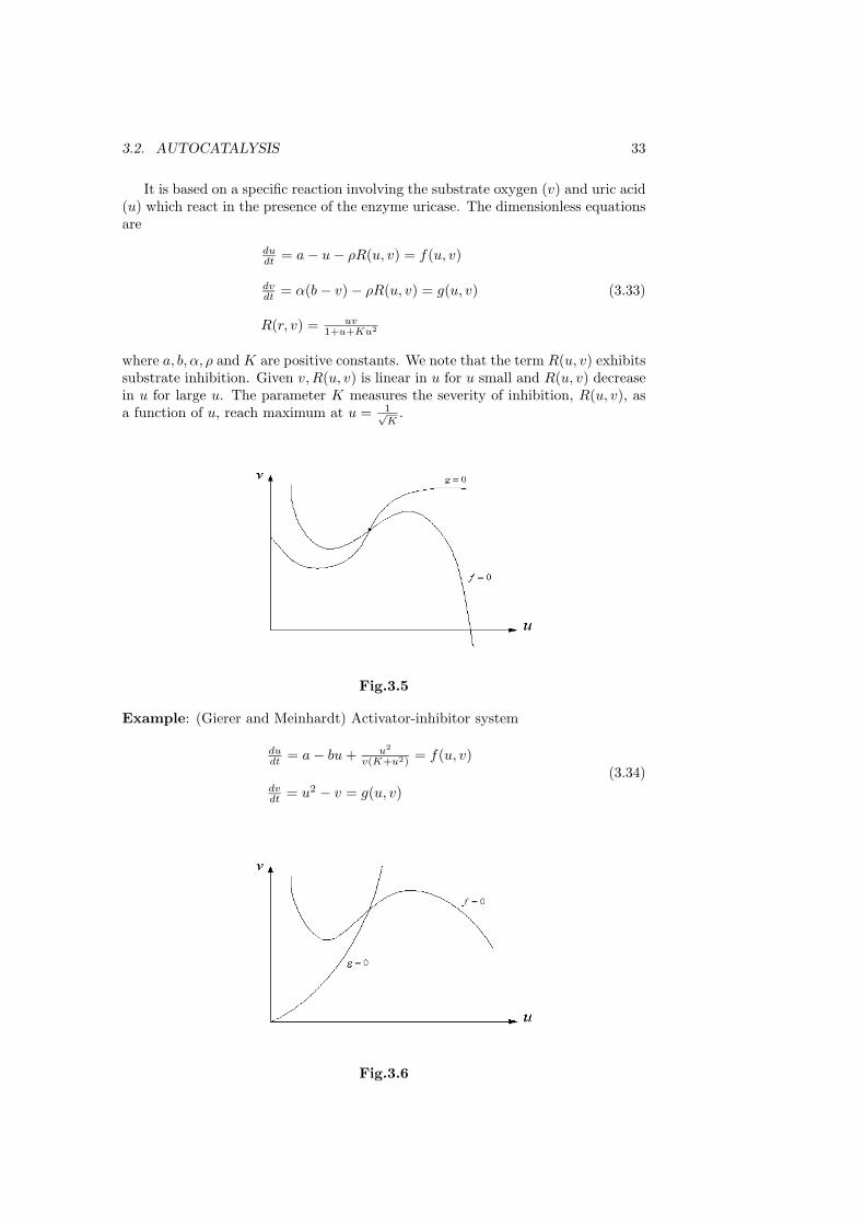
It is based on a specific reaction involving the substrate oxygen (v) and uric acid(u) which react in the presence of the enzyme uricase. The dimensionless equationsare
dudt = a − u − ρR(u, v) = f(u, v)
dvdt = α(b − v) − ρR(u, v) = g(u, v)
R(r, v) = uv1+u+Ku2
(3.33)
where a, b, α, ρ and K are positive constants. We note that the term R(u, v) exhibitssubstrate inhibition. Given v,R(u, v) is linear in u for u small and R(u, v) decreasein u for large u. The parameter K measures the severity of inhibition, R(u, v), asa function of u, reach maximum at u = 1√
K.
Fig.3.5
Example: (Gierer and Meinhardt) Activator-inhibitor system
dudt = a − bu + u2
v(K+u2) = f(u, v)
dvdt = u2 − v = g(u, v)
(3.34)
Fig.3.6
34 CHAPTER 3. CHEMICAL REACTION KINETICS
3.3 Biological Oscillators: Monotone cyclic feed-back systems
In this section we shall consider the biological model in the form of the system ofordinary differential equations
d−→udt
= −→f (−→u ). (3.35)
where ←−u = −→u (t) is the concentration vector. −→f describes the nonlinear reaction
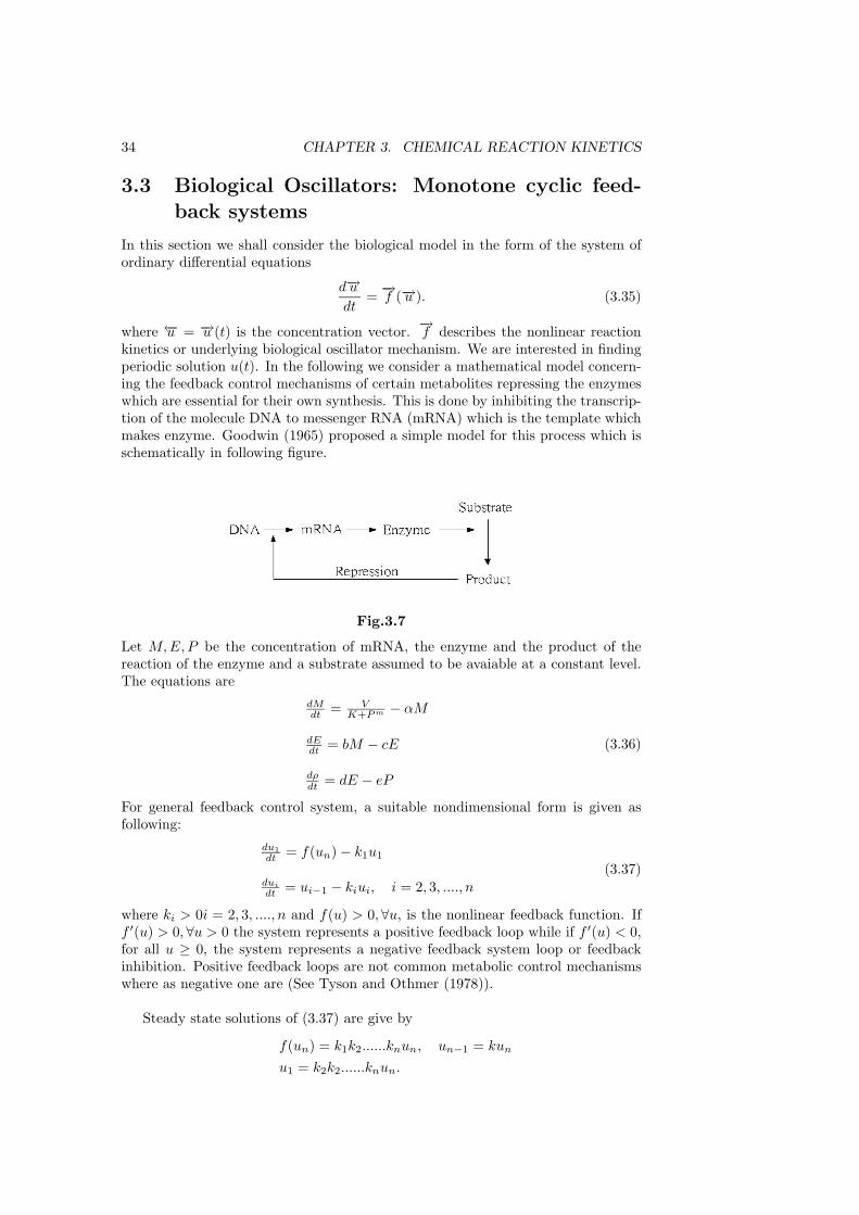
kinetics or underlying biological oscillator mechanism. We are interested in findingperiodic solution u(t). In the following we consider a mathematical model concern-ing the feedback control mechanisms of certain metabolites repressing the enzymeswhich are essential for their own synthesis. This is done by inhibiting the transcrip-tion of the molecule DNA to messenger RNA (mRNA) which is the template whichmakes enzyme. Goodwin (1965) proposed a simple model for this process which isschematically in following figure.
Fig.3.7
Let M,E,P be the concentration of mRNA, the enzyme and the product of thereaction of the enzyme and a substrate assumed to be avaiable at a constant level.The equations are
dMdt = V
K+P m − αM
dEdt = bM − cE
dρdt = dE − eP
(3.36)
For general feedback control system, a suitable nondimensional form is given asfollowing:
du1dt = f(un) − k1u1
dui
dt = ui−1 − kiui, i = 2, 3, ...., n(3.37)
where ki > 0i = 2, 3, ...., n and f(u) > 0,∀u, is the nonlinear feedback function. Iff ′(u) > 0,∀u > 0 the system represents a positive feedback loop while if f ′(u) < 0,for all u ≥ 0, the system represents a negative feedback system loop or feedbackinhibition. Positive feedback loops are not common metabolic control mechanismswhere as negative one are (See Tyson and Othmer (1978)).
Steady state solutions of (3.37) are give by
f(un) = k1k2......knun, un−1 = kun
u1 = k2k2......knun.
3.3. BIOLOGICAL OSCILLATORS: MONOTONE CYCLIC FEEDBACK SYSTEMS35
With positive feedback functions f(u), multiple steady states are possible whereaswith feedback inhibition there is always a unique steady state.
For the more important negative feedback system (3.37), it is quite simple todetermine a bounded domain Ω satisfying −→n · d−→u
dt < 0 for −→u ∈ ∂Ω, i.e., thetrajectory with initial condition in Ω stays in Ω for t ≥ 0. Consider first the twospecies case of (3.37), namely
du1
dt= f(u2) − k1u1
du2
dt= u1 − k2u2
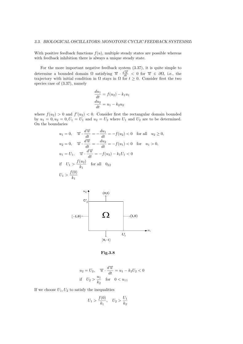
where f(u2) > 0 and f ′(u2) < 0. Consider first the rectangular domain boundedby u1 = 0, u2 = 0, U1 = U1 and u2 = U2 where U1 and U2 are to be determined.On the boundaries
u1 = 0, −→u · d−→udt
= −du1
dt= −f(u2) < 0 for all u2 ≥ 0,
u2 = 0, −→u · d−→udt
= −du2
dt= −f(u1) < 0 for u1 > 0,
u1 = U1, −→u · d−→udt
= −f(u2) − k1U1 < 0
if U1 >f(u2)
k1for all 022
U1 >f(0)k1
Fig.3.8
u2 = U2, −→u · d−→udt
= u1 − k2U2 < 0
if U2 >u1
k2for 0 < u11
If we choose U1, U2 to satisfy the inequalities
U1 >f(0)k1
, U2 >U1
k2

36 CHAPTER 3. CHEMICAL REACTION KINETICS
then the bounded region Ω is positively invariant under the system (3.37). We notethat the unique steady state (u∗
1, u∗2) lies in Ω.
Similarly for n-species negative feedback loop, we can construct a positivelyinvariant, bounded region Ω given by Ω = (u1, ...., un) : 0 ≤ ui ≤ Ui, i = 1, ...., nwhere Ui, i = 1, ...., n satisfy
U1 >f(0)k1
, U2 >U1
k2, ......., Un >
U1
k1k2....kn.
For the large time behavior of (3.37), Mallet-Paret and H. Smidth [?] studiedthe general monotone cyclic feedback systems of the following form
x′i = fi(xi, xi−1), i = 1, 2, ......, n (3.38)
where we agree to interpret x0 as xn. In the cyclic system (3.38) our key assumptionis
δi∂fi
∂xi−1(xi, xi−1) > 0for all xi, xi−1 > 0 (3.39)
for some δi ∈ −1,+1. Thus δi describes whether the effect of xi−1 is to inhibitthe growth of xi(δi = −1) or to augment its growth (δi = +1). The product
= δ1δ2........δn (3.40)
characterizes the entire system as one with negative feedback ( = −1) or positivefeedback ( = +1). We term such a system, of the form (3.38) satisfying (3.39),a monotone cyclic feedback system. In [MS] the authors proved that the Poincare-Bendixson theorem holds for monotone cyclic feedback systems. In particular, theomega-limit set of any bounded orbit of a monotone cyclic feedback system canbe embedded in R2 and must, in fact, be the type encountered in two-dimensionalsystems: either a single equilibrium, a single nonconstant periodic solution, or astructure consisting of a set of equilibria together with homoclinic and hetroclinicorbits connecting these equilibria. In a general sense ”chaos” is ruled out. Theauthors use an integer valued Lyapunov function N as a principal tool. Interestedreaders should consult [].
Besides the single-loop feedback system (3.37), we give the following systems asexamples of (3.38).
Example: Simple Biochemical Control Circuit
y′1 = f(yn) − α1y1
b1+y1
y′i = βiyi−1
ai+yi−1− αiyi
bi+yi, 2 ≤ i ≤ n.
(3.41)
3.4. BIOLOGICAL OSCILLATORS: BELOUSOV-ZHABOTINSKII REACTION37
Example: ([] Banks and Mahaffy) Multigene model with negative feedback
y′1 = f1(wm) − α1y1
y′i = βiyi−1 − αiyi, 2 ≤ i ≤ p
z′1 = f2(yp) − γ1z1
z′j = ηjzj−1 − γjzj , 2 ≤ j ≤ l
w′1 = f3(zl) − δ1w
1
w′k = ξkwk−1 − δ1w
k, 2 ≤ k ≤ m
(3.42)
where αi, βi, γj , ηj , ξk, δk > 0 and f1, f2, f3 satisfies negative feedback assumptionf ′
i(u) < 0 for u ≥ 0, i = 1, 2, 3. This example displace the ”three-gene”. Read-ers may imagine there are n genes where the end procuct of qth gene inhibits thetranscription of mRNA associated with (q + 1)st gene. Delays are sometimes intro-duced in the first terms of the right side of (3.42). One could also replace the linearterms in (3.42) by Michaelis-Menten nonlinearities as in (3.41). We note that J.Mallet-Paret and G. Sell [JDE 1996] proved the Poincare-Bendixson Theorem forthe following Monotone cyclic feedback system with delay:
x′i(t) = fi
(xi(t), xi−1(t − βi)
)(3.43)
3.4 Biological Oscillators: Belousov-Zhabotinskiireaction
In 1951 Belousov found oscillations in the ratio of concentration of the catalyst inthe oxidation of citric acid by bromate. The study of this reaction was continuedby Zhabotiskii (1964) and is now known as the Belousov-Zhabotinskii reaction orsimply the BZ reaction. When the details of this important reaction and some of itsdramatic oscillatory and wave-like properties reached the West in 1970, it provokedwidespread interest and research. Now BZ reaction is considered the prototypechemical oscillator in both theoretical and experimental sense. Here we briefly de-scribe the key steps in the reaction by the Field-Noyes model. The basic mechanismconsists of the oxidation of malonic acid, in an acid medium, by bromate ions, BrO−
3 ,and catalyzed by cerium, which as two state Ce3+ and Ce4+.
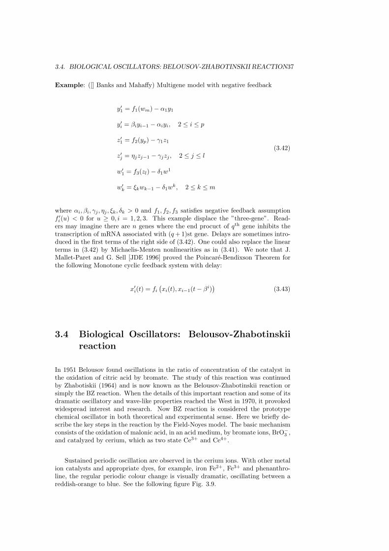
Sustained periodic oscillation are observed in the cerium ions. With other metalion catalysts and appropriate dyes, for example, iron Fe2+, Fe3+ and phenanthro-line, the regular periodic colour change is visually dramatic, oscillating between areddish-orange to blue. See the following figure Fig. 3.9.
38 CHAPTER 3. CHEMICAL REACTION KINETICS
Fig.3.9
In Fig. 3.9. we can see the relaxation oscillations which will be discussed latter.Next we discuss Field-Noyes model or FN model. The key chemical elements in
5-reaction FN model are
X = HBrO2, Y = Br , Z=Ce4+
A = BrO3, P=HOBr
and the model reactions can be approxmated by the sequence
A + Y →k1 X + P, X + Y →k2 2P
A + X →k3 2X + 2Z, 2X →k4 A + P, Z →k5 fY
where the rate constants k1....k5 are known and f is a stoichiometric factor, f ≈ 0.5.We assume the concentration [A] of the bromate ion to be constant. Using the Lawof Mass Action, we obtain
dx
dt= k1ay − k2xy + k3ax − k4x
2
dy
dt= −k1ay − k2xy + fk5z
dz
dt= 2k3ax − k5z
This oscillator system is sometimes referred to as the ”Oregonator” since it exhibitslimit cycle osciaations and research by Field et al was done at the University ofOregon. Following Tyson (1985), introduce
x∗ = xx0
, y∗ = yy0
, z∗ zz0
, t∗ = tt0
x0 = k3ak4
≈ 1.2 × 10⁻⁷M, y0 = k3ak2
≈ 6 × 10⁻⁷M,
z0 = 2(k3a)2
k4k5≈ 5 × 10⁻³M, t0 = 1
k5≈ 50s
ε = k5k3a ≈ 5 × 10⁻⁵, δ = k4k5
k2k3a ≈ 2 × 10⁻⁴
q = k1k4k2k3
≈ 8 × 10⁻⁴, f ≈ 0.5
(3.44)
3.4. BIOLOGICAL OSCILLATORS: BELOUSOV-ZHABOTINSKII REACTION39
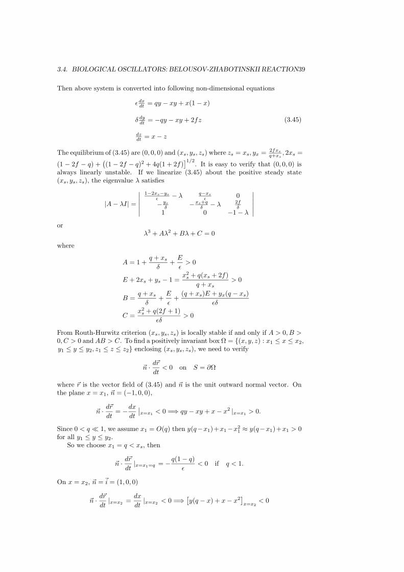
Then above system is converted into following non-dimensional equations
εdxdt = qy − xy + x(1 − x)
δ dydt = −qy − xy + 2fz
dzdt = x − z
(3.45)
The equilibrium of (3.45) are (0, 0, 0) and (xs, ys, zs) where zs = xs, yx = 2fxs
q+xs, 2xs =
(1 − 2f − q) +((1 − 2f − q)2 + 4q(1 + 2f)
]1/2. It is easy to verify that (0, 0, 0) isalways linearly unstable. If we linearize (3.45) about the positive steady state(xs, ys, zs), the eigenvalue λ satisfies
|A − λI| =
∣∣∣∣∣∣1−2xs−ys
ε − λ q−xs
ε 0−ys
δ −xs+qδ − λ 2f
δ1 0 −1 − λ
∣∣∣∣∣∣or
λ3 + Aλ2 + Bλ + C = 0
where
A = 1 +q + xs
δ+
E
ε> 0
E + 2xs + ys − 1 =x2
s + q(xs + 2f)q + xs
> 0
B =q + xs
δ+
E
ε+
(q + xs)E + yx(q − xs)εδ
C =x2
s + q(2f + 1)εδ
> 0
From Routh-Hurwitz criterion (xs, ys, zs) is locally stable if and only if A > 0, B >0, C > 0 and AB > C. To find a positively invariant box Ω = (x, y, z) : x1 ≤ x ≤ x2,y1 ≤ y ≤ y2, z1 ≤ z ≤ z2 enclosing (xs, ys, zs), we need to verify
n · dr
dt< 0 on S = ∂Ω
where r is the vector field of (3.45) and n is the unit outward normal vector. Onthe plane x = x1, n = (−1, 0, 0),
n · dr
dt= −dx
dt
∣∣x=x1 < 0 =⇒ qy − xy + x − x2 |x=x1 > 0.
Since 0 < q 1, we assume x1 = O(q) then y(q−x1)+x1−x21 ≈ y(q−x1)+x1 > 0
for all y1 ≤ y ≤ y2.So we choose x1 = q < xs, then
n · dr
dt|x=x1=q = −q(1 − q)
ε< 0 if q < 1.
On x = x2, n =i = (1, 0, 0)
n · dr
dt|x=x2 =
dx
dt|x=x2 < 0 =⇒ [y(q − x) + x − x2
]x=x2
< 0
40 CHAPTER 3. CHEMICAL REACTION KINETICS
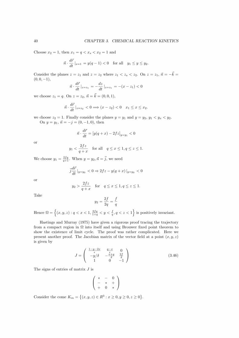
Choose x2 = 1, then x1 = q < xs < x2 = 1 and
n · dr
dt|x=1 = y(q − 1) < 0 for all y1 ≤ y ≤ y2.
Consider the planes z = z1 and z = z2 where z1 < zs < z2. On z = z1, n = −k =(0, 0,−1),
n · dr
dt|z=z1 = −dz
dt|z=z1 = −(x − z1) < 0
we choose z1 = q. On z = z2, n = k = (0, 0, 1),
n · dr
dt|z=z2 < 0 =⇒ (x − z2) < 0 x1 ≤ x ≤ x2.
we choose z2 = 1. Finally consider the planes y = y1 and y = y2, y1 < yx < y2.On y = y1, n = −j = (0,−1, 0), then
n · dr
dt= [y(q + x) − 2fz]y=y1
< 0
or
y1 <2fz
q + xfor all q ≤ x ≤ 1, q ≤ z ≤ 1.
We choose y1 = 2fqq+1 . When y = y2, n = j, we need
jdr
dt|y=y2 < 0 ⇒ 2fz − y(q + x) |y=y2 < 0
or
y2 >2fz
q + xfor q ≤ x ≤ 1, q ≤ z ≤ 1.
Take
y2 =2f
2q=
f
q
Hence Ω =
(x, y, z) : q < x < 1, 2fq1+q < y < f
q , q < z < 1
is positively invariant.
Hastings and Murray (1975) have given a rigorous proof tracing the trajectoryfrom a compact region in Ω into itself and using Brouwer fixed point theorem toshow the existence of limit cycle. The proof was rather complicated. Here wepresent another proof. The Jacobian matrix of the vector field at a point (x, y, z)is given by
J =
⎛⎝ 1−y−2xε
q−xε 0
−y/δ −x+qδ
2fδ
1 0 −1
⎞⎠ (3.46)
The signs of entries of matrix J is⎛⎝ ∗ − 0− ∗ ++ 0 ∗
⎞⎠Consider the come Km =
(x, y, z) ∈ R3 : x ≥ 0, y ≥ 0, z ≥ 0
.
3.4. BIOLOGICAL OSCILLATORS: BELOUSOV-ZHABOTINSKII REACTION41
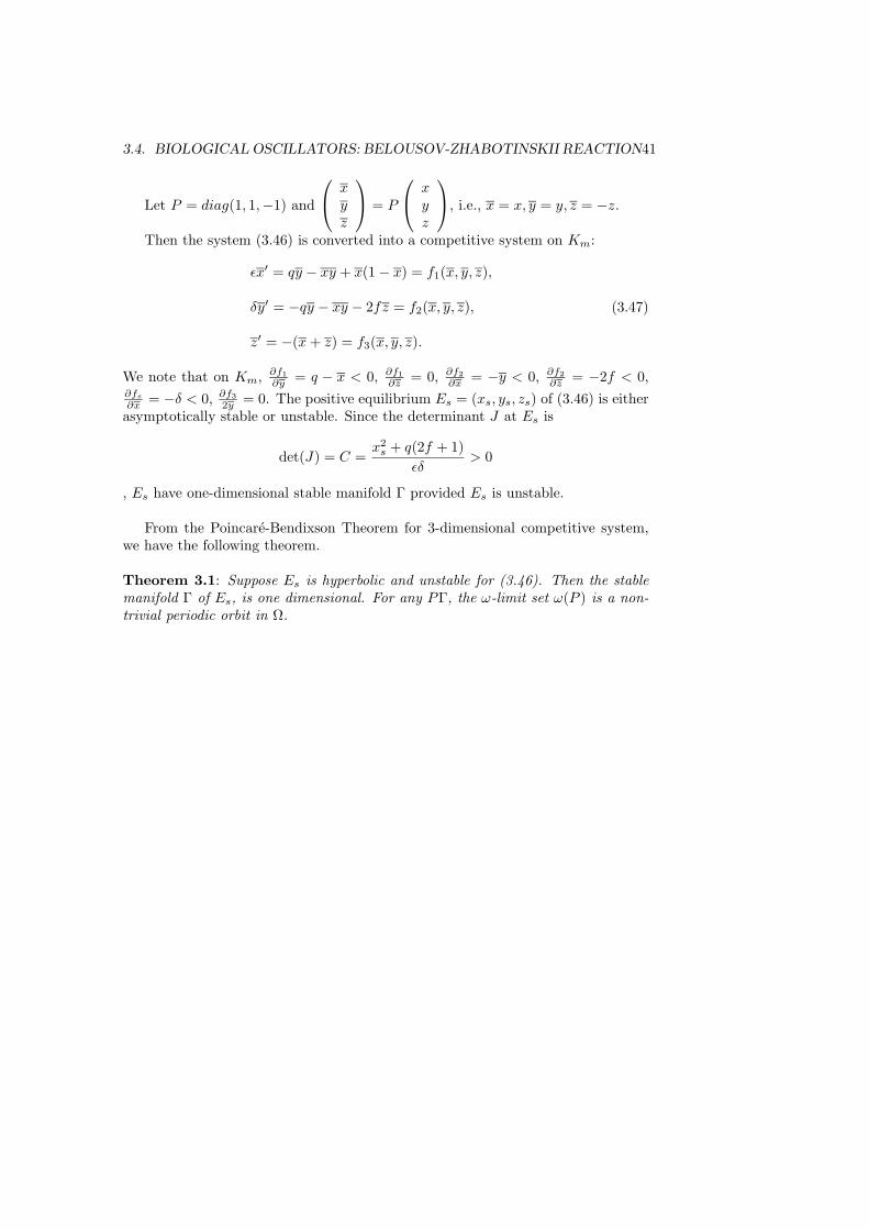
Let P = diag(1, 1,−1) and
⎛⎝ xyz
⎞⎠ = P
⎛⎝ xyz
⎞⎠, i.e., x = x, y = y, z = −z.
Then the system (3.46) is converted into a competitive system on Km:
εx′ = qy − xy + x(1 − x) = f1(x, y, z),
δy′ = −qy − xy − 2fz = f2(x, y, z),
z′ = −(x + z) = f3(x, y, z).
(3.47)
We note that on Km, ∂f1∂y = q − x < 0, ∂f1
∂z = 0, ∂f2∂x = −y < 0, ∂f2
∂z = −2f < 0,∂fs
∂x = −δ < 0, ∂f32y = 0. The positive equilibrium Es = (xs, ys, zs) of (3.46) is either
asymptotically stable or unstable. Since the determinant J at Es is
det(J) = C =x2
s + q(2f + 1)εδ
> 0
, Es have one-dimensional stable manifold Γ provided Es is unstable.
From the Poincare-Bendixson Theorem for 3-dimensional competitive system,we have the following theorem.
Theorem 3.1: Suppose Es is hyperbolic and unstable for (3.46). Then the stablemanifold Γ of Es, is one dimensional. For any PΓ, the ω-limit set ω(P ) is a non-trivial periodic orbit in Ω.

42 CHAPTER 3. CHEMICAL REACTION KINETICS

Chapter 4
Nerve Conduction
In this chapter we shall derive the famous Hodgkin-Huxley model (1952) for whichthey were awarded the Nobel Prize in physiology and medicine in 1963. Hodgkin-Huxley model is too complicated to do mathematical analysis, people instead studythe FitzHugh-Nagumo equations and their variants which extracts the essentialbehavior of the Hodgkin-Huxley fast-slow phase-plane and presents it in a simpliedform.
4.1 Electrical Circuit model of the cell membrane
We may view the cell membrane as a capacitor for its separating charge. Thecapacitance Cm is defined as
Cm =Q
V(4.1)
where Q is the charge across the capacitor and V is the voltage potential necessaryto hold that charge. From standard electrostatics (Coulomb’s law), one can derivethe fact that for two parallel conducting plates separated by an insulator of thicknessd, the capacitance is
Cm =kε0d
(4.2)
where k is the dielectric constant for the insulator and ε0 is the permittivity of freespace. For membrane Cm ≈ 1.0µF/em2, ε0 =
(10−9/(36π)
)F/m, hence it follows
that k ≈ 8.5.A simple electric circuit model of cell membrane is shown in Fig.4.1
Fig.4.1 Electrical circuit model of the cell membrane.
43

44 CHAPTER 4. NERVE CONDUCTION
It is assumed that the membrane acts like a capacitor in parallel with a resistor.Since the current I is defined as dθ
dt , from (4.1) the capacitive current is CmdVdt .
There can be no net buildup of charge on either side of the membrane, the sumof the ionic and capacitive currents must be zero and so
CmdV
dt+ Iion(V, t) = 0 (4.3)
Where V = Vi − Ve, Vi and Ve are internal and external potential of the membranerespectively.
Potential difference across the cell membrane causes ionic currents to flow throughchannels in the cell membrane. Regulation of this membrane potential by controlof ionic channels is the most important for cellular functions. Many cells, suchas neurons and muscle cells, use the membrane potential as a signal and thus theoperation of the nervous system and muscle contraction are both dependent on thegeneration and propagation of electrical signal.
To understand electrical signaling in cells, it is helpful (and not too inaccurate)to divide all cell types into two groups: excitable cells and nonexcitable cells. Manycells maintain a stable equilibrium potential. For some, if currents are applied tothe cell for a short period of time, the potential returns directly to its equilibriumvalue after the applied current is removed. Such cells are called nonexcitable, typicalexamples of which are the epithelial cells that line the walls of the gut. Photore-ceptors are also nonexcitable, although in their case, membrane potential plays anextremely important signaling role nonetheless.
However, there are cells for which, if the applied current is sufficiently strong,the membrane potential goes through a large excursion, called an action potential,before eventually returning to rest. Such cells are called excitable. Excitable cellsinclude cardiac cells, smooth and skeletal muscle cells, secretory cells, and mostneurons. The most obvious advantage of excitability is that an excitable cell eitherresponds in full to a stimulus or not at all, and thus a stimulus of sufficient amplitudemay be reliably distinguished from background noise. In this way, noise is filteredout, and a signal is reliably transmitted.
There are many examples of excitability that occur in nature. A simple exampleof an excitable system is a household match. The chemical components of thematch head are stable to small fluctuations in temperature, but a sufficiently largetemperature fluctuation, caused, for example, by friction between the head and arough surface, triggers the abrupt oxidation of these chemicals with a dramaticrelease of heat and light. The fuse of a stick of dynamite is a one dimensionalcontinuous version of an excitable medium, and a field of dry grass is its two-dimensional version. Both of these spatially extended systems admit the possibilityof wave propagation. The field of grass has one additional feature that the matchand dynamite fuse fail to have, and that is recovery. While it is not very rapid byphysiological standards, given a few months of growth, a burned-over field of grasswill regrow enough fuel so that another fire may spread across it.
Although the generation and propagation of signals have been extensively stud-ied by physiologists for at least the past 100 years, the most important landmark inthese studies is the work of Allan Hodgkin and Andrew Huxley, who developed thefirst quantitative model of the propagation of an electrical signal along a squid giantaxon (deemed ”giant” because of the size of the axon, not the size of the squid).Their model was originally used to explain the action potential in the long giantaxon of a squid nerve cell, but the ideas have since been extended and applied toa wide variety of excitable cells. Hodgkin-Huxley theory is remarkable, not onlyfor its influence on electrophysiology, but also for its influence, after some filtering,

4.1. ELECTRICAL CIRCUIT MODEL OF THE CELL MEMBRANE 45
on applied mathematics. FitzHugh (in particular) showed how the essentials of theexcitable process could be distilled into a simpler model upon which mathematicalanalysis could make some progress, Because this simplified model turned out tobe of such great theoretical interest, it contributed enormously to the formationof a new field of applied mathematics, the study of excitable systems, a field thatcontinues to stimulate a vast amount of research.
Because of the central importance of cellular electrical activity in physiology,because of the importance of the Hodgkin-Huxley model in the study of electricalactivity, and because it forms the basis for the study of excitability, it is no exag-geration to say that the Hodgkin-Huxley model is the most important model in allof the physiological literature.
Hodgkin and Huxley developed the first quantitative model of the propagationof an electrical signal along a squid giant axon. In the squid giant axon, as in manyneural cells, the principal ionic currents are the sodium (Na+) current and thepotassium (K+) current. Although there are other ionic currents, like the chloridecurrent (cl−), H − H theory assume they are small and lumped together into arecurrent called the leakage current. Equation (4.3) becomes
CmdV
dt= −gNa (V − VNa) − gk (V − VK) − gL (V − VL) + Iapp. (4.4)
wheregNa =
INa
V − VNa(Compare with) R =
V
I,
gNa = 1R is the membrane conductance with respect to ionic flow Na+. Similarly
for gK and gL. We may rewrite (4.4) as
CmdV
dt= −geff (V − Veq) + Iapp
where geff = gNa+gK+gL, Veq = (gNaVNa + gKVK + gLVL) /geff , Veq is the mem-brane resting potential and is a balance between the reversal potentials for threeionic currents. In fact, at rest, sodium and leakage conductance are small comparedto potassium conductance, so that the resting potential is closed to potassium equi-librium potential.
Next we want to find the conductance gNa and gK as a function of voltage Vand time t. Hudgkin and Huxley used the voltage clamp to measure the transienttransmembrane current. In Fig.4.2, they found that when the voltage was steppedup and held fixed at a high level, the total ionic current was initial inward, butat later time an outward current developed. They argue that the initial inwardcurrent is carried almost entirely by Na+ ions, while the outward current thatdevelops latter is carried largely by K+ ions. Let’s denote the Na+ currents fortwo cases of normal extra cellular Na+ and zero extracellular Na+ by I ′Na and I2
Na
respectively (INa = I ′Na + I2Na and
I ′Na/I2Na ≡ K ≡ constant.
Since Iion = INa + IK , I ′K = I2K , it follows that I ′ion − I ′Na = I2
ion − I2Na
(I ′K = I2
K
)and thus
I ′Na =K
K − 1(I ′ion − I2
ion)(I ′ion − I2
ion = I ′Na − I2Na = I ′Na − 1
KI ′Na =
K − 1K
I ′Na
)
46 CHAPTER 4. NERVE CONDUCTION
and
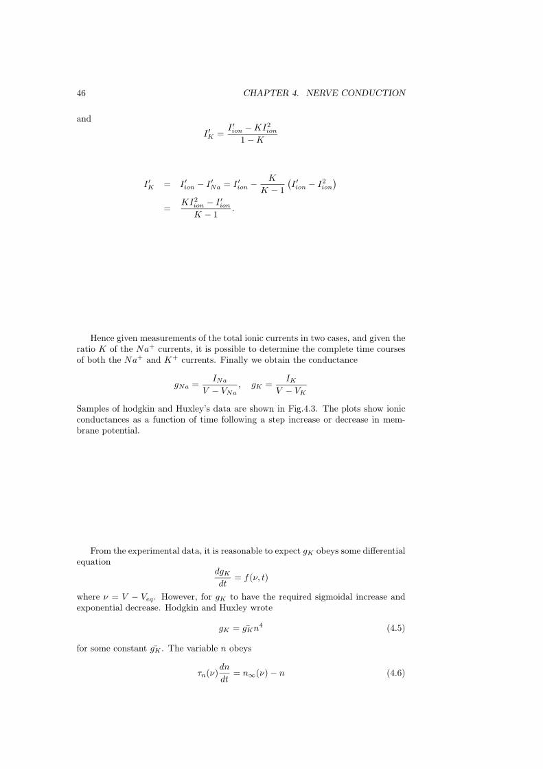
I ′K =I ′ion − KI2
ion
1 − K
I ′K = I ′ion − I ′Na = I ′ion − K
K − 1(I ′ion − I2
ion
)=
KI2ion − I ′ion
K − 1.
Hence given measurements of the total ionic currents in two cases, and given theratio K of the Na+ currents, it is possible to determine the complete time coursesof both the Na+ and K+ currents. Finally we obtain the conductance
gNa =INa
V − VNa, gK =
IK
V − VK
Samples of hodgkin and Huxley’s data are shown in Fig.4.3. The plots show ionicconductances as a function of time following a step increase or decrease in mem-brane potential.
From the experimental data, it is reasonable to expect gK obeys some differentialequation
dgK
dt= f(ν, t)
where ν = V − Veq. However, for gK to have the required sigmoidal increase andexponential decrease. Hodgkin and Huxley wrote
gK = gKn4 (4.5)
for some constant gK . The variable n obeys
τn(ν)dn
dt= n∞(ν) − n (4.6)
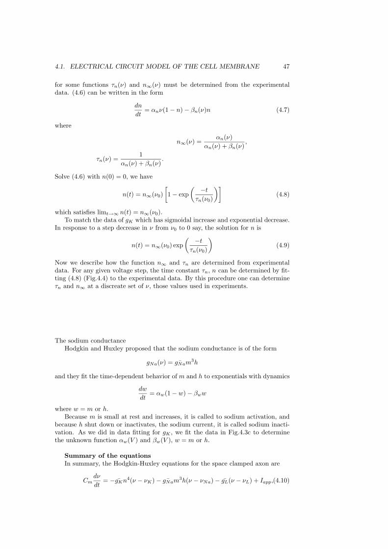
4.1. ELECTRICAL CIRCUIT MODEL OF THE CELL MEMBRANE 47
for some functions τn(ν) and n∞(ν) must be determined from the experimentaldata. (4.6) can be written in the form
dn
dt= αnν(1 − n) − βn(ν)n (4.7)
where
n∞(ν) =αn(ν)
αn(ν) + βn(ν),
τn(ν) =1
αn(ν) + βn(ν).
Solve (4.6) with n(0) = 0, we have
n(t) = n∞(ν0)[1 − exp
( −t
τn(ν0)
)](4.8)
which satisfies limt→∞ n(t) = n∞(ν0).To match the data of gK which has sigmoidal increase and exponential decrease.
In response to a step decrease in ν from ν0 to 0 say, the solution for n is
n(t) = n∞(ν0) exp( −t
τn(ν0)
)(4.9)
Now we describe how the function n∞ and τn are determined from experimentaldata. For any given voltage step, the time constant τn, n can be determined by fit-ting (4.8) (Fig.4.4) to the experimental data. By this procedure one can determineτn and n∞ at a discreate set of ν, those values used in experiments.
The sodium conductanceHodgkin and Huxley proposed that the sodium conductance is of the form
gNa(ν) = ¯gNam3h
and they fit the time-dependent behavior of m and h to exponentials with dynamics
dw
dt= αw(1 − w) − βww
where w = m or h.Because m is small at rest and increases, it is called to sodium activation, and
because h shut down or inactivates, the sodium current, it is called sodium inacti-vation. As we did in data fitting for gK , we fit the data in Fig.4.3c to determinethe unknown function αw(V ) and βw(V ), w = m or h.
Summary of the equationsIn summary, the Hodgkin-Huxley equations for the space clamped axon are
Cmdν
dt= −gKn4(ν − νK) − ¯gNam3h(ν − νNa) − gL(ν − νL) + Iapp,(4.10)
48 CHAPTER 4. NERVE CONDUCTION
dm
dt= αm(1 − m) − βmm, (4.11)
dn
dt= αn(1 − n) − βnn, (4.12)
dh
dt= αh(1 − h) − βhh. (4.13)
The specific functions α and β proposed by Hodgkin and Huxley were, in units of(ms)−1,
αm = 0.125 − ν
exp(
25−ν10
)− 1, (4.14)
βm = 4 exp(−ν
18
), (4.15)
αh = 0.07 exp(−ν
20
), (4.16)
βh =1
exp(
30−ν10
)+ 1
, (4.17)
αn = 0.0110 − ν
exp(
10−ν10
)− 1, (4.18)
βn = 0.125 exp(−ν
80
). (4.19)
For these expressions, the potential ν is the deviation from rest (V = Veq + ν),measured in units of mV , current density is in units of /cm2, conductances are inunits of mS/cm2, and capacitance is in units of /cm2. The remaining constants are
¯gNa = 120, gK = 36, gL = 0.3, (4.20)
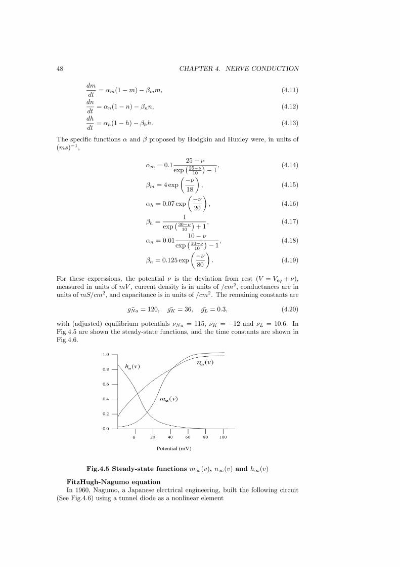
with (adjusted) equilibrium potentials νNa = 115, νK = −12 and νL = 10.6. InFig.4.5 are shown the steady-state functions, and the time constants are shown inFig.4.6.
Fig.4.5 Steady-state functions m∞(v), n∞(v) and h∞(v)
FitzHugh-Nagumo equationIn 1960, Nagumo, a Japanese electrical engineering, built the following circuit
(See Fig.4.6) using a tunnel diode as a nonlinear element
4.1. ELECTRICAL CIRCUIT MODEL OF THE CELL MEMBRANE 49
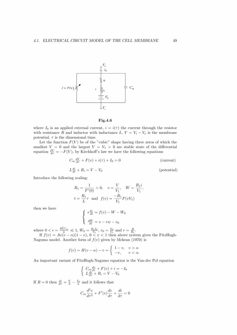
Fig.4.6
where I0 is an applied external current, i = i(τ) the current through the resistorwith resistance R and inductor with inductance L, V = Vi − Ve is the membranepotential, τ is the dimensional time.
Let the function F (V ) be of the ”cubic” shape having three zeros of which thesmallest V = 0 and the largest V = V1 > 0 are stable state of the differentialequation dV
dτ = −F (V ), by Kirchhoff’s law we have the following equations
CmdVdτ + F (v) + i(τ) + I0 = 0 (current)
L didt + Ri = V − V0 (potential)
Introduce the following scaling:
R1 =1
F ′(0)> 0, v =
V
V1, W =
R1i
V1,
t =R1
Lτ and f(v) =
−R1
V1F (vV1)
then we have ⎧⎨⎩εdv
dt = f(v) − W − W0
dWdt = v − rw − v0
where 0 < ε = R21Cm
L 1, W0 = R1I0V1
, v0 = V0V1
and r = RR1
.If f(v) = Av(v − α)(1 − v), 0 < v < 1 then above system gives the FitzHugh-
Nagumo model. Another form of f(v) given by Mckean (1970) is
f(v) = H(v − α) − v =
1 − v, v > α−v, v < α.
An important variant of FitzHugh-Nagumo equation is the Van-der Pol equationCm
dvdτ + F (v) + i = −I0
L didτ + Ri = V − V0
If R = 0 then didτ = V
L − V0L and it follows that
Cmd2v
dτ2+ F ′(v)
dv
dτ+
di
dτ= 0

50 CHAPTER 4. NERVE CONDUCTION
or
Cmd2v
dτ2+ F ′(v)
dv
dτ+
v
L=
V0
L
Set F (v) = A(
v3
3 − v)
and from the rescaling, we obtain Van der Pol equation
v′′ + a(v2 − 1
)v′ + v = 0

Chapter 5
Reaction diffusion equations
5.1 Simple random walk and derivation of the dif-fusion equation
Consider one-dimensional random walk. Suppose a particle moves randomly backand forwarded along a line in a fixed step x that are taken in a fixed time t.Let p(m,n) be the probability that a particle reaches a point m space steps to theright (i.e. x = mx) after n time steps (i.e. after a time nt), where n ∈ Z+ and−n ≤ m ≤ n. Let us suppose that to reach mx it has moved a steps to the rightand b to the lift. Then
m = a − b, a + b = n
Then a = n+m2 , b = n − a.
The number of possible paths that a particle can reach this point x = mx is
n!a!b!
=n!
a!(n − a)!≡ Cn
a
The total number of possible n-step paths is 2n and so the probability p(m,n) is
p(m,n) =12n
n!a!(n − a)!
, a =n + m
2
n + m is even.Note that from binomial theorem
n∑m=−n
p(m,n) =n∑
a=0
Cna
(12
)n−a(12
)a
= 1
p(m,n) is the binomial distribution.From Stirling’s formula
n! (2πn)12 nne−n, as n → ∞,
p(m,n)[
2πn
] 12 exp[−m2
2n
], m 1, n 1. (Exercises)
Setmx = x, nt = t
with x, t fixed and m → ∞, n → ∞, x → 0, t → 0. Then p(m,n) → 0 asm,n → ∞ and it is not the quantity of interest. Let u = p
2x . Then u2x is the
51
52 CHAPTER 5. REACTION DIFFUSION EQUATIONS
probability of find a particle in the interval (x, x + x) at time t. With m = xx ,
n = tt ,
u =p(
xx , t
t
)2x
[ t
(2π · t · |x)2
] 12
exp[
x2t
2t(x)2
].
If we assume
limx → 0t → 0
(x)2
2t→ D
then
u(x, t) = limx → 0t → 0
p(
xx , t
t
)2x
=(
14πDt
) 12
exp(− x2
4Dt
). (5.1)
D is the diffusion coefficient. It is a measure of how effectively the particles dispersefrom a high to a low density. For example in blood, haemoglobin molecules hasdiffusion coefficient of order 10−7cm2/sec while for oxggen in blood is of order of10−5cm2/sec.
Now we consider the classical approach to diffusion, namely, Fickian diffusion.Let J be the flux of material (cells, chemical etc). Then J is proportional to thegradient of the concentration of the materials. That is
J ∝ − ∂c
∂xor J = −D
∂c
∂x
where c(x, t) is the concentration of the species and D is the diffusivity. The minussign indicates the diffusion transports matter from a high to a low concentration.Consider a small region x0 < x < x1 = x0 + x. Then
∂
∂t
∫ x1
x0
c(x, t)dx = J(x0, t) − J(x1, t).
If x → 0 then we obtain
∂c
∂t= −∂J
∂x=
∂(D ∂c
∂x
)∂x
.
If D is a constant then∂c
∂t= D
∂2c
∂x2(5.2)
Let c(x, 0) = Qδ(x) then the solution of PDE
c(x, t) =Q
2 (πDt)12e−
x24Dt
If Q = 1 then we obtain the same result as (5.1) from a random walk.Now we relate the random walk to the diffusion equation (5.2). Let p(x, t) be
the probability that a particle released at x = 0 at t = 0 reach x in time t. At timet −t the particle was at x −x or x + x. Thus if α and β are the probabilitythat a particle will move to the right or left
p(x, t) = αp(x −t, t −t) + βp(x + x, t −t)α + β = 1
5.2. REACTION DIFFUSION EQUATIONS 53
If α = β = 12 i.e. the random walk is isotropic (no bias) then Taylor expansion at
(x, t) yields∂p
∂t=
(x)2
2t
∂2p
∂x2+(t
2
)∂2p
∂t2+ ...
Now let x → 0 and t → 0 s.t
limx → 0t → 0
(x)2
2t= D
we get∂p
∂t= D
∂2p
∂x2
5.2 Reaction diffusion equations
Consider diffusion in three space dimensions. Let S be an arbitary surface enclosinga volume V . Then we have rate of change of amount in V equals to rate of flow ofmaterial across S into V plus the material created in V .
∂
∂t
∫V
c(x, t)dV = −∫
S
J · ds +∫
V
f · dV
By divergence Theorem∫V
[∂c
∂t+ D · J − f(c, x, t)
]dv = 0.
Since V is arbitary, we obtain the reaction diffusion equation
∂c
∂t+ ∇ · J = f(c, x, t) (5.3)
Now J = −D∇c then (5.3) becomes
∂c
∂t= ∇ · (D∇c) + f (5.4)
The system of reaction-diffusion equation is
∂u
∂t= f + ∇ · (D∇u)
where D is a matrix of diffusives and u(x, t) ∈ Rk.
5.3 Chemotaxis
A large number of insects and animals rely on an acute sense of smell for conveyinginformation between members of the species. Chemicals which are involved in thisprocess are called pheromones. For example, the female silk moth Bombyxmoriexudes a pheromone, called bombykol, as a sex attractant for the male, which hasa remarkably efficient antenna filter to measure the bombykol concentration, and itmoves in the direction of increasing concentration. The modelling problem here isa fascinating and formidable one (Murray 1977). The acute sense of smell of many
54 CHAPTER 5. REACTION DIFFUSION EQUATIONS
deep sea fish is particularly important for communication and predation. Other thanfor territorial demarcation the simplest important exploitation of pheromone releaseis the directed movement it can generate in the population. Here we model thischemically directed movement, that is chemotaxis, which, unlike diffusion, directsthe motion up a concentration gradient.
It is not only in animal and insect ecology that chemotaxis is important. Itcan be equally crucial in biological processes where there are numerous examples.For example when a bacterial infection invades the body it may be attacked bymovement of cells towards the source as a result of chemotaxis. Convincing evi-dence suggests that leukocyte cells in the blood move towards a region of bacterialinflammation, to counter it, by moving up a chemical gradient caused by the infec-tion (see, for example, Lauffenburger and Keller 1979, Tranquillo and Lauffenburger1986, 1988, Alt and Lauffenburger 1987).
A widely studied chemotactic phenomenon is that exhibited by the slime moldDictyostelium discoideum where single-cell amoebae move towards regions of rela-tively high concentrations of a chemical called cyclic-AMP which is produced bythe amoebae themselves. Interesting wave-like movement and spatial patterning areobserved experimentally. A discussion of the phenomenon and some of the math-ematical models which have been proposed together with some analysis are given,for example, in the book by Segel (1984). The kinetics involved have been modelledby several outhors. As more was found out about the biological system the modelschanged. Recently new, more complex and more biologically realistic models havebeen proposed by Martiel and Goldbeter (1987) and Monk and Othmer (1989).Both of these new models exhibit oscillatory behaviour.
Let us suppose that the presence of a gradient in an attractant, a(x, t), givesrise to a movement, of the cells say, up the gradient. The flux of cells will increasewith the number of cells, n(x, t), present. Thus we may reasonably take as thechemotactic flux
J = nχ(a)∇a, (5.5)
where χ(a) is a function of the attractant concentration. In the general conservationequation for n(x, t), namely
∂n
∂t+ ∇ · J = f(n),
where f(n) represents the growth term for the cells, the flux
J = Jdiffusion + Jchemotaxis
where the diffusion contribution is from (5.4) with the chemotaxis flux from (5.5).Thus the reaction (or population) diffusion-chemotaxis equation is
∂n
∂t= f(n) −∇ · nχ(a)∇a + ∇ · D∇n. (5.6)
where D is the diffusion coefficient of the cells.Since the attractant a(x, t) is a chemical it also diffuses and is produced, by the
amoebae for example, so we need a further equation for a(x, t). Typically
∂a
∂t= g(a, n) + ∇ · Da∇a, (5.7)
where Da is the diffusion coefficient of a and g(a, n) is the kinetics/source term,which may depend on n and a. Normally we would expect Da > D. If several
5.3. CHEMOTAXIS 55
species or cell types all respond to the attractant the governing equation for thespecies vector is an obvious generalization of (9.28) to a vector form with χ(a)probably different for each species.
In the slime mold model of Keller and Segel (1971), g(a, n) = hn − ka whereh ,k are positive constants. Here hn represents the spontaneous production of theattractant and is proportional to the number of amoebae n, while-ka representsdecay of attractant activity: that is there is an exponential decay if the attractantis not produced by the cells.
One simple version of the model has f(n) = 0: that is the amoebae productionrate is negligible. This is the case during pattern formation phase in the mold’s lifecycle. The chemotactic term χ(a) is taken to be a positive constant χ0. The formof this term in any case is speculative. With constant diffusion coefficients, togetherwith the above linear form for g(a, n), the model in one space dimension becomesthe nonlinear system
∂n∂t = D ∂2n
∂x2 − χ0∂∂x
(∂a∂x
),
∂a∂t = hn − ka + Da
∂2a∂x2
(5.8)
Other forms have been proposed for the chemotactic factor χ(a). For example
χ(a) =χ0
a, χ(a) =
χ0K
(K + a)2, χ0 > 0, K > 0 (5.9)
which are known respectively as the log law and receptor law. In there, as a de-creases the chemotactic effect increases.

56 CHAPTER 5. REACTION DIFFUSION EQUATIONS
Appendix A
Let m = (m1,m2, ....,mn) where mi ∈ 0, 1 and
Km = x ∈ Rn : (−1)mixi ≥ 0, 1 ≤ i ≤ n .
Km is a cone in Rn and it generates a partial order ≤m defined by x ≤m y ifand only if y − x ∈ Km. Equivalently xi ≤ yi for those i for which mi = 0 andyi ≤ xi for those i for which mi = 1. Let P be the diagonal matrix defined byP = diag ((−1)m1 , ....., (−1)mn). Obviously P = P−1 and x ≤m y if and only ifPx ≤ Py. The domain D is said to be Pm-convex if tx + (1 − t)y ∈ D wheneverx, y ∈ D, 0 < t1 and x ≤m y. We say x′ = f(x) is cooperative with respective toKm provided D is Pm-convex and
(−1)mi+mj∂fi
∂xj(x) ≥ 0, i = j, x ∈ D. (A.1)
It is competitive with respect to Km if
(−1)mi+mj∂fi
∂xj(x) ≤ 0, i = j, x ∈ D. (A.2)
Proposition A.1: Let D be Pm-convex and f is continuously differentiable vectorfield on D such that (A.1) holds. If x ≤m y, t > 0 and the flow ϕt(x) and ϕt(y) aredefined, then ϕt(x) ≤m ϕt(y). If (A.2) holds then similar conclusions are valid fort > 0.
Proof: Let g(y) = Pf(Py), y ∈ PD. Then vector field g generates a flow ψt definedby ψt(y) = Pϕt(Py). Since gi(y) = (−1)mifi(Py), ∂gi
∂yj(y) = (−1)mi+mj ∂fi
∂xj(Py) ≥ 0
by (A.1). If x ≤m y, it follows that Px ≥ Py then by Prop 1.1[], ψt(Px) ≤ ψt(Py).This implies ϕt(x) ≤m ϕt(y) as asserted. The other assertions follows similarly.
Proposition A.1 suggests an algorithm for determining whether a given systemx′ = f(x) is cooperative or competitive in a domain D with respect to one of thecomes Km. First we check the off-diagonal elements of the Jacobian matrix aresign-stable in D. This means that each i = j either (a) ∂fi
∂xj(x) ≥ 0 for all x ∈ D
or (b) ∂fi
∂xj(x) ≤ 0 for all x ∈ D. Assuming this test is passed, then the Jacobian
matrix must be tested for sign-symmetry: ∂fi
∂xj(x)∂fj
∂xi(y) ≥ 0 for all x = j, x, y ∈ D.
If this test is satisfied, then for each i < j set sij = 0 if ∂fi
∂xj(x) + ∂fj
∂xi(x) > 0 for
some x ∈ D. sij = 1 if ∂fi
∂xj(x) + ∂fj
∂xi(x) < 0 for some x ∈ D. Now consider the
system of n(n − 1)/2mi + mj = sij(mod 2), i < j
57

58 APPENDIX A.
Solve m and we find the cone Km. Consider the graph G with vertices 1, 2, ...., nwhere an undirected edge connects vertices i and j if ∂fi
∂xj(x) or ∂fj
∂xi(x) does not
vanish identically in D. Attach a sign + or - to the edge. Then x′ = f(x) is coop-erative in D with respect some cone Km if and only if every closed loop in G thenumber of edges with - signs is even. It is competitive if every loop in G has an oddnumber of edges with - signs.
For system (3.45), from (3.46), the graph is
Relaxation oscillations in BZ reaction: [ ] p.193Consider FN model (3.45)
εdxdt = qy − xy + x(1 − x)
δ dydt = −qy − xy + 2fz (3.45)
dzdt = x − z
with dimensionless parameters given by (3.44). Note that ε δ and we set εdxdt ≈ 0.
This gives
x = x(y) =(1 − y) +
[(1 − y)2 + 4qy
] 12
2(A.3)
Then (3.45) is reduced to
δ dydt = 2fz − y [x(y) + q]
dzdt = x(y) − z
(A.4)
From (3.48) with q 1, the z-nullcline of (3.49) is
z = x(y) ≈
1 − y for q 1 − y ≤ 1qy
y−1 for q y − 1.(A.5)
Then y-nullcline is
z =y [x(y) + q]
2f≈
⎧⎪⎨⎪⎩y(1−y)
2f for q 1 − y 1y[ qy
y−1+q]2f q y − 1
qyf y 1
(A.6)
Then we have the following figures of relaxzation oscillation.
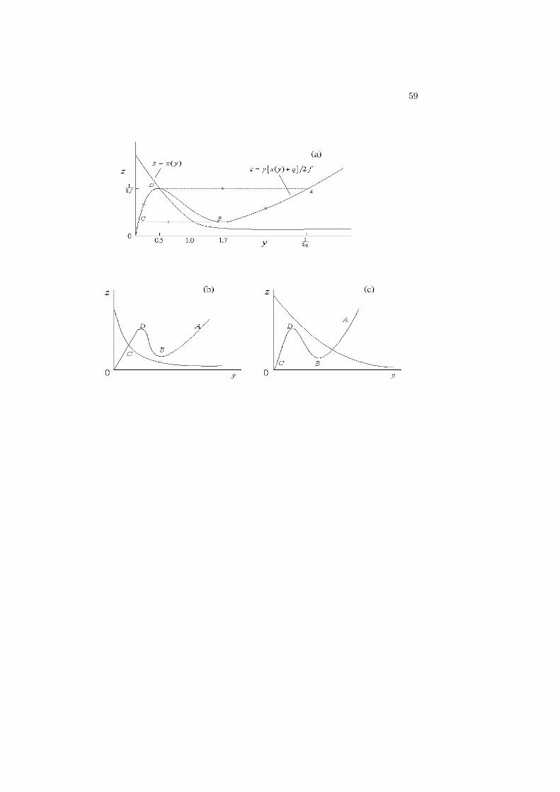
59

60 APPENDIX A.

Bibliography
[C] K. S. Cheng: Uniqueness of limit cycle of a predator-prey system, SIAM J.Math. Analysis (1981).
[Co] Coppel: Stability and Asymptotic Behavior of Differential Equations, Heath,Boston 1965.
[H] J. Hale: Functional Differential Equations.
[H1] J. Hale: Ordinary differential equations.
[HH1] S. B. Hsu and T. W. Hwang: Global stability for a class of Predator-PreySystem, SIAM J. Appl. Math, 1995 p.763-783.
[HH2] S. B. Hsu and T. W. Hwang: Uniqueness of limit cycles for a predator-preysystem of Holling and Lesile type, Canadian Applied Math. Quarterly (1998)Vol.6, No.2, p.91-117.
[HHK] S. B. Hsu, T. W. Hwang, Y. Kuang: Global Analysis of the Michaelis-Menten type ratio-dependence predator-prey system, J. Math. Biology,42(2001) 489-506.
[HHW] Hsu Hubbell Waltman: Competing of predators, SIAM J. Appl. Math.(1978) p.617-625.
[Hirsch 1] Hirsch: Systems of differential equations which are competitive or coop-erative I. limit sets, SIAM J. Appl. Math(1982) 167-179.
[Hirsch 2] Hirsch: Systems of differential equations which are competitive or coop-erative III. Competing species, Nonlinearity (1988) 51-71.
[Hsu] S. B. Hsu: Limiting behavior of competing species, SIAM J. Applied Math.1978, p.760-763.
[M] ] J. Murray: Mathematical Biology.
[MG] Mackey and Glass: Oscillations and chaos in physiological control systems,Science 197, 287-289(1977).
[R] Rosenzweig: Paradox of enrichment: destablization of exploitation systems inecological time, Science 171 (1969) p.385.
[S] H. Smith: Monotone Dynamical System.
61