Mathematical Models of Cognitive

Control: Design, Comparison, and

Optimization

Stephanie Eileen Goldfarb

A Dissertation

Presented to the Faculty

of Princeton University

in Candidacy for the Degree

of Doctor of Philosophy

Recommended for Acceptance

by the Department of

Mechanical and Aerospace Engineering

Advisers: Philip Holmes and Naomi Ehrich Leonard

April 2013

c© Copyright by Stephanie Eileen Goldfarb, 2013.

All rights reserved.

Abstract

In this thesis, we investigate human decision making dynamics in a series of

simple perceptual decision making tasks. The level of caution with which a human

subject responds to stimuli is of central interest, since it influences the speed and

accuracy of responses. We study the role of caution parameters in models of

cognitive control processes.

We first investigate the influence of stimulus likelihood on human error dynam-

ics in sequential two-alternative choice tasks. Errors are understood to increase

in frequency when caution is low. When subjects repeatedly discriminate between

two stimuli, their error rates and mean reaction times (RTs) systematically de-

pend on prior sequences of stimuli. We analyze sequential effects on RTs, showing

that relationships among prior stimulus sequences and the corresponding RTs for

correct trials, error trials, and averaged over all trials are significantly influenced

by the probability of alternations. Finally, we show that simple, sequential up-

dates to the initial condition and thresholds of a pure drift diffusion model (DDM)

can account for the trends in RT for correct and error trials. Our results suggest

that error-based parameter adjustments are critical to modeling sequential effects.

These relationships have not been captured by previous models.

In the remainder of the thesis, we compare models of human choice dynamics

in tasks in which subjects must trade off between speed and accuracy in order to

maximize reward rates. Caution is of critical importance: while errors decrease

in frequency as caution increases, decision time increases. Direct manipulation

of caution provides a framework with which to compare models. Recent work

has compared the predictions of the Linear Ballistic Accumulator (LBA) and the

iii

DDM for simple RT tasks but has identified no important qualitative differences

between the predictions of the two models. Comparing the fits of the two models

for simple RT tasks in which subjects attempt to maximize reward rate, we show

that while the pure DDM predicts a single optimal performance curve, the curve

for the LBA varies significantly with model parameters. Critically, we find that

while reward seeking behavior is predicted on average by an increase in caution in

the DDMs, the same behavior in the best-fitting LBA model is instead predicted

by a decrease in caution.

iv

Acknowledgements

First and foremost, I would like to thank my advisers Phil Holmes and Naomi

Leonard for their support and encouragement over the past five years. What I

have learned from each of you at Princeton goes far beyond techniques. Phil, you

have shown me such brilliance, diligence, and patience-thank you for so generously

pouring through manuscripts with me for hours, allowing me a window into the

great care with which you pursue your written endeavors. With each discussion,

read-through, or re-write with you, I gained new insights and clarity. Writing on

my own now, I will miss all of your neat and constructive handwritten comments!

I have developed considerably more as a reader, writer and thinker from these

interactions than perhaps from any other experience I have had at Princeton.

Working on writing with you has marked some of the times I felt most fully engaged

and connected to my research work and to the scientific community. Naomi,

your enthusiasm is contagious and your storytelling captivating; your periodic

encouragement and review of both the big picture and the fine details with me,

with insight and creativity, has done much to propel me to push harder on problems

on which I have been stuck. I hope that I am able to similarly encourage individuals

I may supervise or mentor in the future, and I plan to try to emulate much of your

approach to mentoring students.

I would also like to thank my reader Michael Littman for his invaluable com-

ments and suggestions on this thesis, as well as my committee members Jonathan

Cohen and Robert Stengel for support throughout the PhD process. Jon, thank

you also for providing me with feedback and encouragement as well as a steady

flow of ideas at the weekly Wednesday morning meetings. I feel as if I have reaped

v

many of the benefits of being your student, although I was not formally your ad-

visee. Without your input this thesis in its current form would not exist. Rob,

thank you for patiently teaching me loads about giving a research presentation by

reviewing materials with me slide by slide early on in my Princeton career; the

experience guides me to this day.

It takes a village to raise a graduate student. My intellectual development has

been fostered by the many members of the Holmes and Leonard groups, past and

present. In particular, thank you to my graduate student peers in this process:

Andrea Nedic, Andy Stewart, Ben Nabet, Dan Swain, Darren Pais, George Young,

Josh Proctor, Juan Gao, Katie Fitch, Kendra Cofield, Paul Reverdy, Raghu Kukil-

laya, Sam Feng, Tian Shen, and Will Scott. The mentoring of postdocs has been

truly a blessing. In particular: Bob Wilson, Damon Tomlin, Elliott Ludvig, Fuat

Balci, KongFatt Wong-Lin, Marieke van Vugt, Mike Schwemmer, and Pat Simen.

KongFatt, thank you for tirelessly supporting me through my preparation for the

qualifying exams. Without you, my qualification for this degree would have been

much less solid. Alex Olshevsky and Carlos Caicedo, I look forward to staying in

touch with each of you and consider you very good friends as well as role models.

Alex, thank you for the many thought provoking discussions in the wee hours of

the morning. Carlos, thank you for the steady supply of jokes and encouragement

and for later helping me complete my proofs via Skype from your new home in

the UK. The next time I see you, I will have some better pranks ready! Thanks

also goes to my peers in the Cohen group Andra Geana, John White, and Michael

Todd.

My other Princeton colleagues and friends have been similarly indispensi-

ble. Within the Mechanical Engineering Department: Alexis Carlotti, Chrissy

vi

Peabody, Dan Sirbu, Dmitry Savransky, Elizabeth Young, Eric Cady, Ismaiel

Yakub, Jing Du, Mac Haas, Michael Burke, Nick Kattamis, Tyler Groff... Thank

you to many of you for keeping me company over all of the beers I failed to drink!

Outside of MAE, I’d like to thank: Sushobhan for challenging me to be a

better and a stronger person. Madhur for listening with so much insight and

understanding. Aman and Abhishek for their friendship, humor, and hospitality.

Jeff for teaching me so much about food and friendship. June for listening patiently

over so many pints of frozen yogurt. Victor and Daline for helping me find so much

joy in dance, music, life... I’m also thankful to have Anna, Coach Tom, Dalal,

Daniel, Eugene, Farahnaz, Gaurav, Gonzalo, Jeff, Joe, Kevin, Lorne, Michael,

Sally, Schubert, Shyam, Sibren, Tanushree, Tracy, Wenzhe, and Yanhua in my

life.

The McGraw Center for Teaching and Learning at Princeton has provided me

with excellent support. At McGraw, I’m especially grateful for Nic, Jeff, and

Sandy and to my fellow Teaching Fellows, Ashley and Geneva.

My time at Princeton was also given shape and meaning from extracurricular

work with the Graduate Women in Science and Engineering group. I’m especially

grateful for the mentoring of alumni Cheryl Rowe-Rendleman, Kristin Epstein,

and Cathy Haupt and the support of Deans Stephen Friedfeld and Brandi Jones,

as well as of Jo Kelly and Alex Calcado.

My Princeton career began years before I set foot on campus. I am grateful

for the teaching and mentoring of Emmett O’Brien, Mark Campbell, Mark Psiaki,

Norman Bucknor, Paul Dawson, Richard Rand, and Venkatesh Rao early in my

career. I am fortunate also for my enduring friendships with Cara, Dan, Dora,

Holly, Kelly, Matt, Morgan, Sarah, Shreenath, and Tom.

vii

The journey to this point would have been infinitely more painful without my

wonderful family. In particular: Mom, you have always wanted the best for me, and

I am very grateful to never have doubted your dedication, affection, or intentions.

Everything you did was out of love. To my beloved father, your memory inspires

me, and I hope that you would be proud of me and the woman I have become.

I see pieces of you - and pieces of myself - when I spend time with your half of

the family. My grandmother, Alice, has taught me so much about the importance

of love, family, and tradition. My Grandpa David has taught me about the fierce

preciousness of life. To my Aunt Beth, Aunt Margie and Uncle Rickey, Uncle

Julian, Uncle Sam and Aunt Aviva, Uncle Ken and Aunt Amy, Aunt Diane, my

many cousins, and my maternal grandparents, thank you for always believing in

me.

viii

“I get by with a little help from my friends.”

-The Beatles

To my friends.

ix

Contents

Abstract . . . . . . . . . . . . . . . . . . . . . . . . . . . . . . . . . . . . iii

Acknowledgements . . . . . . . . . . . . . . . . . . . . . . . . . . . . . . v

List of Tables . . . . . . . . . . . . . . . . . . . . . . . . . . . . . . . . . xii

List of Figures . . . . . . . . . . . . . . . . . . . . . . . . . . . . . . . . . xiii

1 Introduction 1

1.1 Survey of Related Work . . . . . . . . . . . . . . . . . . . . . . . . 6

1.2 Model Comparison Metrics . . . . . . . . . . . . . . . . . . . . . . . 11

1.3 Main Contributions of Dissertation . . . . . . . . . . . . . . . . . . 12

1.4 Outline of Dissertation . . . . . . . . . . . . . . . . . . . . . . . . . 14

2 Responses to Unbiased Random Stimuli 16

2.1 Materials and methods . . . . . . . . . . . . . . . . . . . . . . . . . 19

2.1.1 Experiment 1: Unbiased random stimuli . . . . . . . . . . . 19

2.1.2 An adapted drift diffusion model . . . . . . . . . . . . . . . 20

2.1.3 Model simulation and data fitting procedure . . . . . . . . . 25

2.2 Results . . . . . . . . . . . . . . . . . . . . . . . . . . . . . . . . . . 27

2.3 Discussion . . . . . . . . . . . . . . . . . . . . . . . . . . . . . . . . 34

2.4 Appendix: Derivation of RTs for Correct and Error Trials . . . . . . 35

x

3 Responses to Biased Random Stimuli 38

3.1 Materials and methods . . . . . . . . . . . . . . . . . . . . . . . . . 41

3.1.1 Experiment 2: Biased Random Stimuli . . . . . . . . . . . . 41

3.1.2 Comparing model fits . . . . . . . . . . . . . . . . . . . . . . 44

3.2 Results . . . . . . . . . . . . . . . . . . . . . . . . . . . . . . . . . . 45

3.3 Discussion . . . . . . . . . . . . . . . . . . . . . . . . . . . . . . . . 52

4 Responses to Stimuli in Reward Maximization Tasks 56

4.1 Introduction . . . . . . . . . . . . . . . . . . . . . . . . . . . . . . . 56

4.2 Methods . . . . . . . . . . . . . . . . . . . . . . . . . . . . . . . . . 61

4.2.1 Comparing Processes: Drift Diffusion and Linear Ballistic

Accumulation . . . . . . . . . . . . . . . . . . . . . . . . . . 61

4.2.2 Optimal Performance in the Models . . . . . . . . . . . . . . 66

4.2.3 Reward Maximization Experiment . . . . . . . . . . . . . . 74

4.2.4 Data Fitting Procedures . . . . . . . . . . . . . . . . . . . . 75

4.3 Results . . . . . . . . . . . . . . . . . . . . . . . . . . . . . . . . . . 77

4.4 Discussion . . . . . . . . . . . . . . . . . . . . . . . . . . . . . . . . 88

4.5 Appendix . . . . . . . . . . . . . . . . . . . . . . . . . . . . . . . . 91

5 Conclusion and Future Directions 100

5.1 Discussion . . . . . . . . . . . . . . . . . . . . . . . . . . . . . . . . 102

5.2 Future Work . . . . . . . . . . . . . . . . . . . . . . . . . . . . . . . 103

Bibliography 106

xi

List of Tables

2.1 DDM Parameterization for Experiment 1 . . . . . . . . . . . . . . . 27

2.2 Model Peformance Comparison . . . . . . . . . . . . . . . . . . . . 33

3.1 Comparison of DDM Parameterizations . . . . . . . . . . . . . . . . 45

4.1 DDM and LBA Model Fit Comparison . . . . . . . . . . . . . . . . 78

xii

List of Figures

1.1 Two alternative forced choice (TAFC) task protocol. . . . . . . . . 7

1.2 Comparison of popular decision models. . . . . . . . . . . . . . . . 15

2.1 Mean RTs and ERs for unbiased random stimuli. . . . . . . . . . . 28

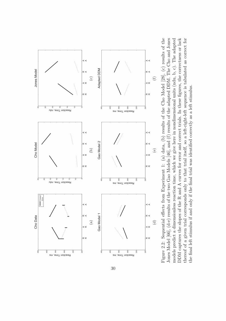
2.2 Sequential effects from Experiment 1: comparison of participant

data and several model fits. . . . . . . . . . . . . . . . . . . . . . . 30

2.3 Sequential RT tradeoff for unbiased tasks: a slower RT for correct

trials corresponds to a faster RT for error trials for the sequences

RR, AR, RA, and AA. . . . . . . . . . . . . . . . . . . . . . . . . . 31

2.4 Post-error slowing in data from Experiment 1 and in the models of

Cho [28], Jones [66], Gao [46], and the adapted DDM of the present

study. . . . . . . . . . . . . . . . . . . . . . . . . . . . . . . . . . . 33

3.1 Transition-oriented Markov process. . . . . . . . . . . . . . . . . . . 41

3.2 Mean RTs and ERs for biased random stimuli. . . . . . . . . . . . . 47

3.3 Adapted DDM fits to RT data for correct and error trials for re-

sponses to biased random stimuli. . . . . . . . . . . . . . . . . . . . 49

xiii

3.4 Sequential RT tradeoff for biased random stimuli: mean RTs for

correct trials are strongly correlated with mean RTs for error trials

for each of the sequences RR, AR, RA, AA. . . . . . . . . . . . . . 51

3.5 Post-error slowing for biased random stimuli data and model fit. . . 52

4.1 Sample Optimal Performance Curves (OPCs) for the pure and ex-

tended DDMs. . . . . . . . . . . . . . . . . . . . . . . . . . . . . . . 69

4.2 Sample Optimal Performance Curves (OPCs) for the LBA Model. . 71

4.3 Comparison of AIC, AICc, and BIC scores for DDM and LBA model

fits. . . . . . . . . . . . . . . . . . . . . . . . . . . . . . . . . . . . . 80

4.4 Comparative data and fits to the OPC for high and low performing

participants. . . . . . . . . . . . . . . . . . . . . . . . . . . . . . . . 82

4.5 Mean data and fits to the OPC, averaged over all participants. . . . 83

4.6 Mean threshold parameter values for the three DDM fits, averaged

by difficulty condition. . . . . . . . . . . . . . . . . . . . . . . . . . 84

4.7 Mean threshold parameter values differ significantly for the two

LBA Model fits. . . . . . . . . . . . . . . . . . . . . . . . . . . . . 85

4.8 Mean values of the range of initial conditions, by model and diffi-

culty condition. . . . . . . . . . . . . . . . . . . . . . . . . . . . . 86

4.9 Mean values of the drift rate parameter. . . . . . . . . . . . . . . . 87

4.10 Comparison of data and fits to RT, in ms, by participant and diffi-

culty condition. . . . . . . . . . . . . . . . . . . . . . . . . . . . . 93

4.11 Comparison of data and fits to ER, by participant and difficulty

condition. . . . . . . . . . . . . . . . . . . . . . . . . . . . . . . . . 94

xiv

4.12 Comparison of RR data (total rewards earned in Sessions 10-13) by

participant and difficulty condition. . . . . . . . . . . . . . . . . . . 95

4.13 Model fits to mean normalized DT and ER data for each difficulty

condition and participant. . . . . . . . . . . . . . . . . . . . . . . . 96

4.14 Comparison of values of the caution or threshold parameter in the

different model fits, by participant and difficulty condition. . . . . . 97

4.15 Mean values of the variability in initial conditions, separated by

participant, model, and difficulty condition. . . . . . . . . . . . . . 98

4.16 Mean values of the drift parameter, µ, separated by participant,

model, and difficulty condition. . . . . . . . . . . . . . . . . . . . . 99

xv

Chapter 1

Introduction

The challenge of integrating teams of human and robotic agents is of growing inter-

est. A positive consequence of the long recognized, steadily increasing capabilities

of machines [76, 105, 29] is a large and growing set of ways to employ a machine

to assist or even replace an individual or group in the completion of a task [129].

In order to better integrate human and robotic agents in task completion, our

understanding of the human operator must keep pace with our understanding of

machines.

The work presented in this thesis is motivated by the problem of understanding

the behavior of the human operator in tasks shared between humans and robots.

Our specific focus is upon developing a better understanding of the human operator

herself while performing simple and time-sensitive tasks. In particular, given a

human operator and several machines, or a combination of humans and machines,

characteristic patterns of human behavior such as variations in speed and accuracy

are of interest.

1

We will focus on a special case of this human-robot system, in which one human

operator must make multiple simple decisions quickly. For example, a pilot must

make rapid decisions in the cockpit regarding how to turn and navigate around

obstacles in her field of view [67]. Similarly, racecar drivers on the track and to a

lesser extent, drivers on a public highway must deftly navigate a series of obstacles,

determining the speed at which and the side from which to pass other cars [37]. In

such situations, errors frequently incur a significant cost [101, 108]. In the case of

military operations, the cost may be measured in lives saved or lost [131]. Systems

whose evolution is governed by interactions and feedback among human and robot

operators and the environment are known as human-in-the-loop (HITL) systems

[36, 68].

The design of these HITL systems can be informed by the relative abilities of

human and robotic agents. In general, human agents perform better at varied and

interesting tasks and tend to stall or commit errors on more mundane tasks [34].

In contrast, a computer can excel at the simplest and most tedious tasks, such as

sorting data or performing mathematical operations, but it will frequently struggle

to process novel or unprecedented situations. However, for successful completion

of several tedious tasks, such as image and text recognition in captchas, some

human supervision is necessary. Conversely, certain very difficult tasks (e.g. chess

[80, 24], go [13, 77], image recognition [60]) can be performed well by a computer

alone when significant computing resources are allocated. Tasking the human is

generally imperative but the optimal way to do so is unclear. Moreover, the design

of a system with both human and robotic participants can deeply benefit from an

understanding of the ways humans and robots react to environmental stimuli.

2

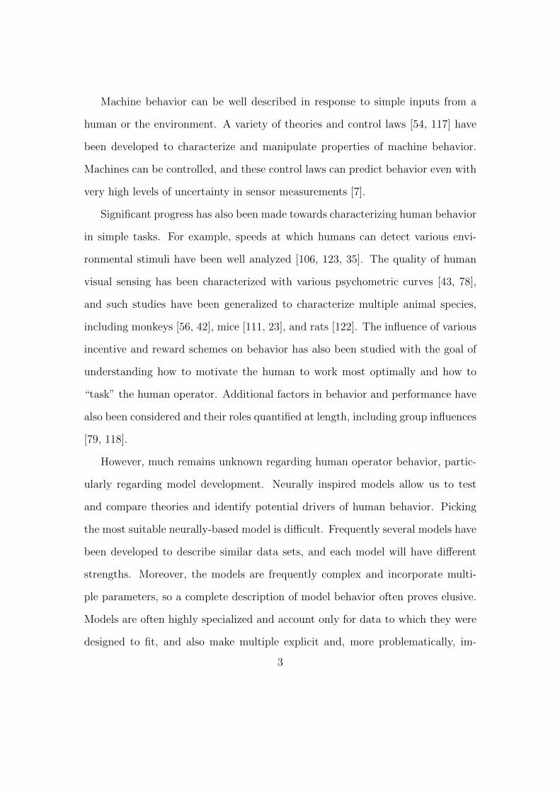
Machine behavior can be well described in response to simple inputs from a

human or the environment. A variety of theories and control laws [54, 117] have

been developed to characterize and manipulate properties of machine behavior.

Machines can be controlled, and these control laws can predict behavior even with

very high levels of uncertainty in sensor measurements [7].

Significant progress has also been made towards characterizing human behavior

in simple tasks. For example, speeds at which humans can detect various envi-

ronmental stimuli have been well analyzed [106, 123, 35]. The quality of human

visual sensing has been characterized with various psychometric curves [43, 78],

and such studies have been generalized to characterize multiple animal species,

including monkeys [56, 42], mice [111, 23], and rats [122]. The influence of various

incentive and reward schemes on behavior has also been studied with the goal of

understanding how to motivate the human to work most optimally and how to

“task” the human operator. Additional factors in behavior and performance have

also been considered and their roles quantified at length, including group influences

[79, 118].

However, much remains unknown regarding human operator behavior, partic-

ularly regarding model development. Neurally inspired models allow us to test

and compare theories and identify potential drivers of human behavior. Picking

the most suitable neurally-based model is difficult. Frequently several models have

been developed to describe similar data sets, and each model will have different

strengths. Moreover, the models are frequently complex and incorporate multi-

ple parameters, so a complete description of model behavior often proves elusive.

Models are often highly specialized and account only for data to which they were

designed to fit, and also make multiple explicit and, more problematically, im-

3

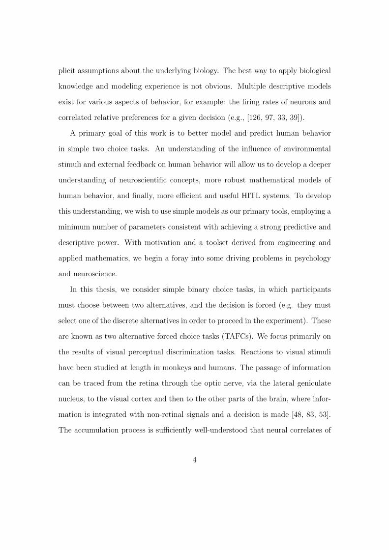
plicit assumptions about the underlying biology. The best way to apply biological

knowledge and modeling experience is not obvious. Multiple descriptive models

exist for various aspects of behavior, for example: the firing rates of neurons and

correlated relative preferences for a given decision (e.g., [126, 97, 33, 39]).

A primary goal of this work is to better model and predict human behavior

in simple two choice tasks. An understanding of the influence of environmental

stimuli and external feedback on human behavior will allow us to develop a deeper

understanding of neuroscientific concepts, more robust mathematical models of

human behavior, and finally, more efficient and useful HITL systems. To develop

this understanding, we wish to use simple models as our primary tools, employing a

minimum number of parameters consistent with achieving a strong predictive and

descriptive power. With motivation and a toolset derived from engineering and

applied mathematics, we begin a foray into some driving problems in psychology

and neuroscience.

In this thesis, we consider simple binary choice tasks, in which participants

must choose between two alternatives, and the decision is forced (e.g. they must

select one of the discrete alternatives in order to proceed in the experiment). These

are known as two alternative forced choice tasks (TAFCs). We focus primarily on

the results of visual perceptual discrimination tasks. Reactions to visual stimuli

have been studied at length in monkeys and humans. The passage of information

can be traced from the retina through the optic nerve, via the lateral geniculate

nucleus, to the visual cortex and then to the other parts of the brain, where infor-

mation is integrated with non-retinal signals and a decision is made [48, 83, 53].

The accumulation process is sufficiently well-understood that neural correlates of

4

visual discrimination TAFCs have been directly recorded from single and multiple

neurons in monkeys (e.g., [81, 16, 104, 120]).

Within the visual discrimination TAFC framework, we may then address two

questions of interest:

• Can we predict and model human behavior?

• How does this behavior relate to its physiological correlates?

With regard to the first question, that of predicting behavior, we consider how

quickly and accurately human participants can identify environmental stimuli.

The process is influenced by stimulus likelihoods as well as by reward or incentive

schemes. To address the two factors, we first analyze data from two experiments

which manipulate stimulus structure, and then from an experiment which incor-

porates performance-based rewards. We develop a simple, biologically-plausible

account for human behavior in each of the tasks.

In total, we look closely at three identification and classification tasks, each

requiring sequential discrimination between two discrete alternatives. The first

task serves as a control in which subjects must only discriminate between each set

of two alternatives presented to them, and in which the stimulus alternatives are

presented in an unbiased random order. In the next task, a bias is introduced to

the order of stimulus presentation. Finally, in the third of the tasks, correct and

timely completion of the task is rewarded, so that subjects must attempt to trade

off speed and accuracy in a manner which optimizes their rate of reward.

With regard to the second question, that of connecting physical behavior to

its neural correlates, we consider a variety of modeling and physical studies. In

particular, we consider adaptations of the pure drift diffusion model [47, 94, 51, 10],

5

which has been shown to mimic aspects of neural integration. We then can refer

to our model to explain trends in behavior based on both the data and the model

fits.

The structure of the remainder of this chapter is as follows. First, we provide

a more detailed survey of related work, including both biophysical models and the

experiments which motivated them. We then identify a series of metrics used to

evaluate models, and which we will use to compare our models to those presented

in other work. After that, we summarize our main contributions and provide an

outline of the dissertation.

1.1 Survey of Related Work

In this section, we consider the standard two alternative forced choice task (TAFC)

framework, and the data collected during such an experimental task. We then

describe several models in the literature which connect behavior and its neural

correlates.

A typical TAFC proceeds as follows. Participation in the study begins with

the administration of instructions, which may be followed by one or more training

sessions. After the subject has completed these preliminary exercises, her formal

participation in the experiment begins. At the beginning of each trial, a stimulus

is presented to the subject. Common stimuli include visual representations such

as stationary alphanumeric characters [28, 135], shapes [124, 9], or moving dots

[18, 58]. After the stimulus is presented, the subject must then respond by indi-

cating the chosen alternative, which she is generally instructed to do by pressing a

button or, if eye trackers are used, initiating a saccade to a visual target. After the

6

subject responds, a response to stimulus interval (RSI) is initiated. The RSI may

be either constant or selected from a distribution of RSIs, such as an exponential

distribution. After the RSI has passed, the process is repeated with the presen-

tation of a new stimulus. In the experiments studied here, several hundred trials

form a block during which experimental conditions such as stimulus probabilities

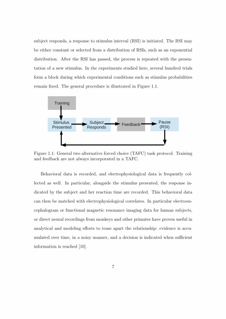
remain fixed. The general procedure is illustrated in Figure 1.1.

Training

Stimulus Presented

SubjectResponds

Pause(RSI)Feedback

Figure 1.1: General two alternative forced choice (TAFC) task protocol. Trainingand feedback are not always incorporated in a TAFC.

Behavioral data is recorded, and electrophysiological data is frequently col-

lected as well. In particular, alongside the stimulus presented, the response in-

dicated by the subject and her reaction time are recorded. This behavioral data

can then be matched with electrophysiological correlates. In particular electroen-

cephalogram or functional magnetic resonance imaging data for human subjects,

or direct neural recordings from monkeys and other primates have proven useful in

analytical and modeling efforts to tease apart the relationship: evidence is accu-

mulated over time, in a noisy manner, and a decision is indicated when sufficient

information is reached [10].

7

Modeling efforts take advantage of these correlations between decision making

behavior and the neural recordings. We briefly summarize below a few common

models. We will consider these models in greater detail in the following chapters.

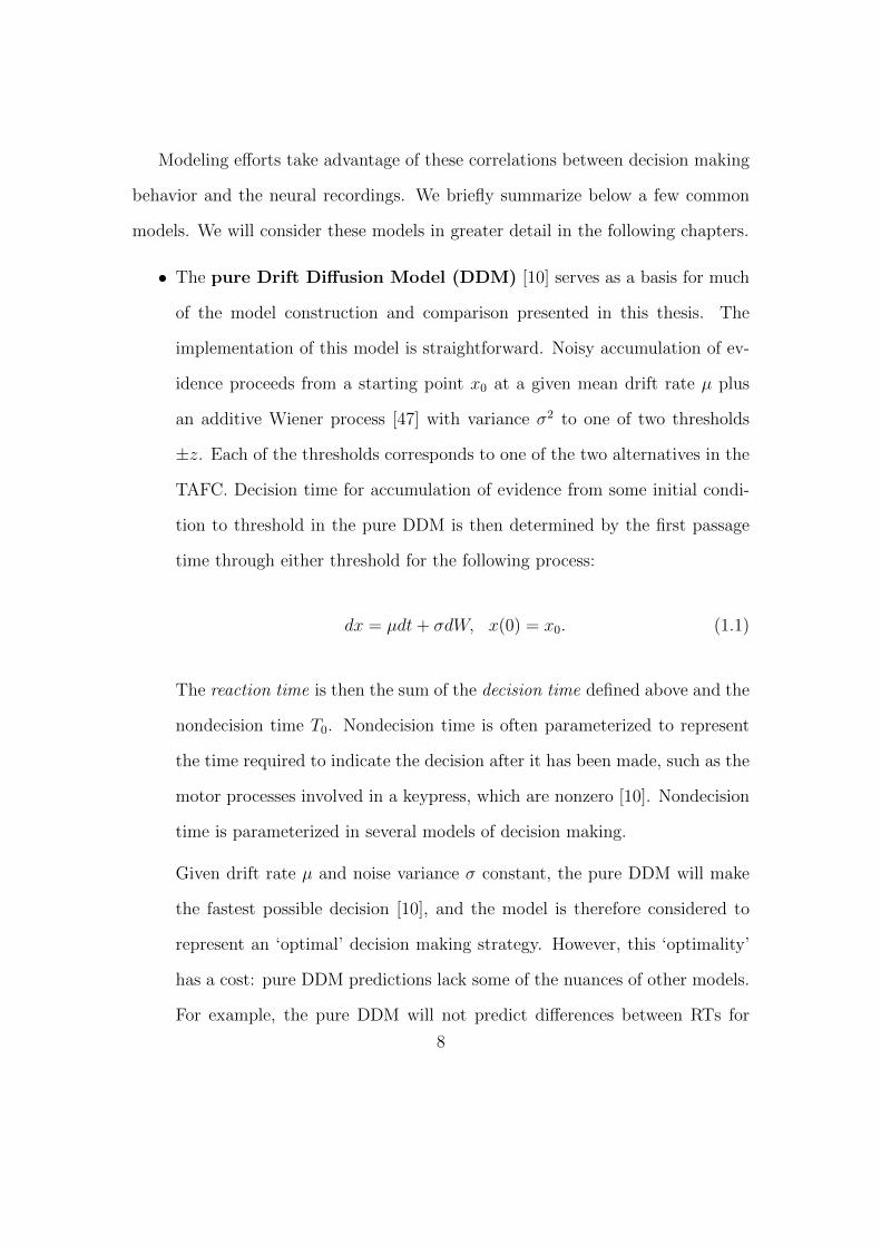
• The pure Drift Diffusion Model (DDM) [10] serves as a basis for much

of the model construction and comparison presented in this thesis. The

implementation of this model is straightforward. Noisy accumulation of ev-

idence proceeds from a starting point x0 at a given mean drift rate µ plus

an additive Wiener process [47] with variance σ2 to one of two thresholds

±z. Each of the thresholds corresponds to one of the two alternatives in the

TAFC. Decision time for accumulation of evidence from some initial condi-

tion to threshold in the pure DDM is then determined by the first passage

time through either threshold for the following process:

dx = µdt+ σdW, x(0) = x0. (1.1)

The reaction time is then the sum of the decision time defined above and the

nondecision time T0. Nondecision time is often parameterized to represent

the time required to indicate the decision after it has been made, such as the

motor processes involved in a keypress, which are nonzero [10]. Nondecision

time is parameterized in several models of decision making.

Given drift rate µ and noise variance σ constant, the pure DDM will make

the fastest possible decision [10], and the model is therefore considered to

represent an ‘optimal’ decision making strategy. However, this ‘optimality’

has a cost: pure DDM predictions lack some of the nuances of other models.

For example, the pure DDM will not predict differences between RTs for

8

error or correct trials, and it may not be able to capture individual RT dis-

tributions. To account for observed variability in RTs, additional variability

in the DDM model parameters is required.

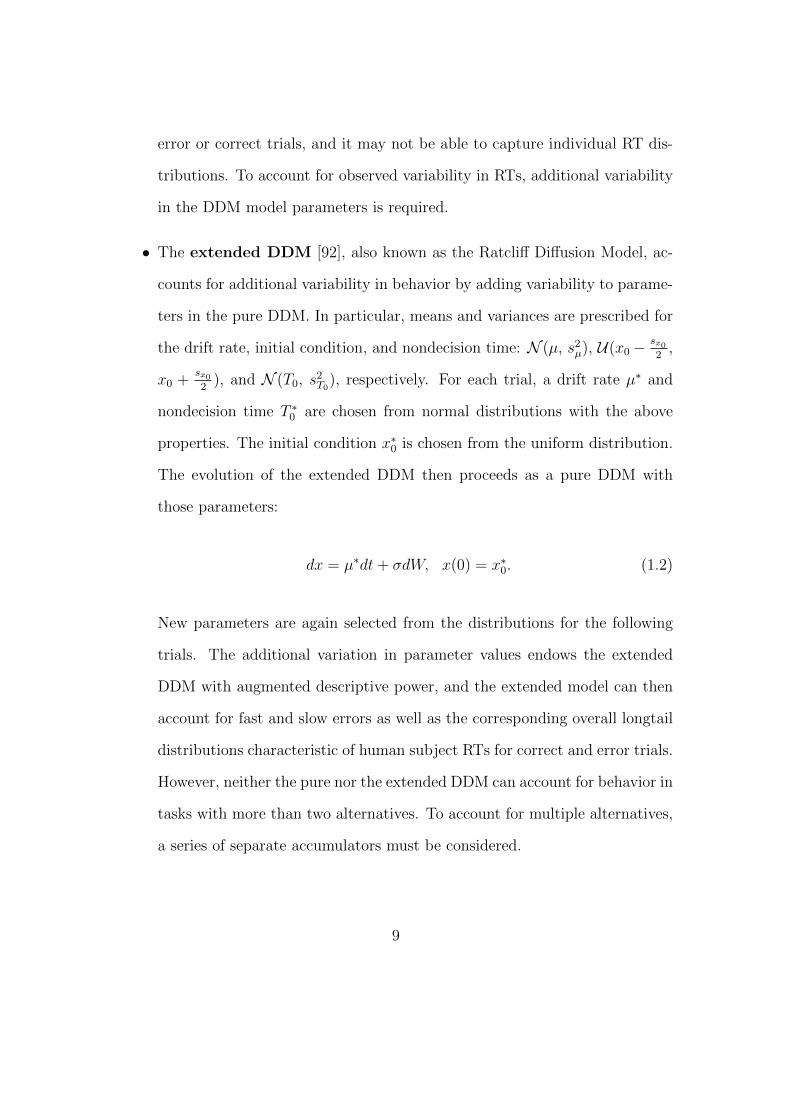
• The extended DDM [92], also known as the Ratcliff Diffusion Model, ac-

counts for additional variability in behavior by adding variability to parame-

ters in the pure DDM. In particular, means and variances are prescribed for

the drift rate, initial condition, and nondecision time: N (µ, s2µ), U(x0− sx0

2,

x0 +sx02

), and N (T0, s2T0

), respectively. For each trial, a drift rate µ∗ and

nondecision time T ∗0 are chosen from normal distributions with the above

properties. The initial condition x∗0 is chosen from the uniform distribution.

The evolution of the extended DDM then proceeds as a pure DDM with

those parameters:

dx = µ∗dt+ σdW, x(0) = x∗0. (1.2)

New parameters are again selected from the distributions for the following

trials. The additional variation in parameter values endows the extended

DDM with augmented descriptive power, and the extended model can then

account for fast and slow errors as well as the corresponding overall longtail

distributions characteristic of human subject RTs for correct and error trials.

However, neither the pure nor the extended DDM can account for behavior in

tasks with more than two alternatives. To account for multiple alternatives,

a series of separate accumulators must be considered.

9

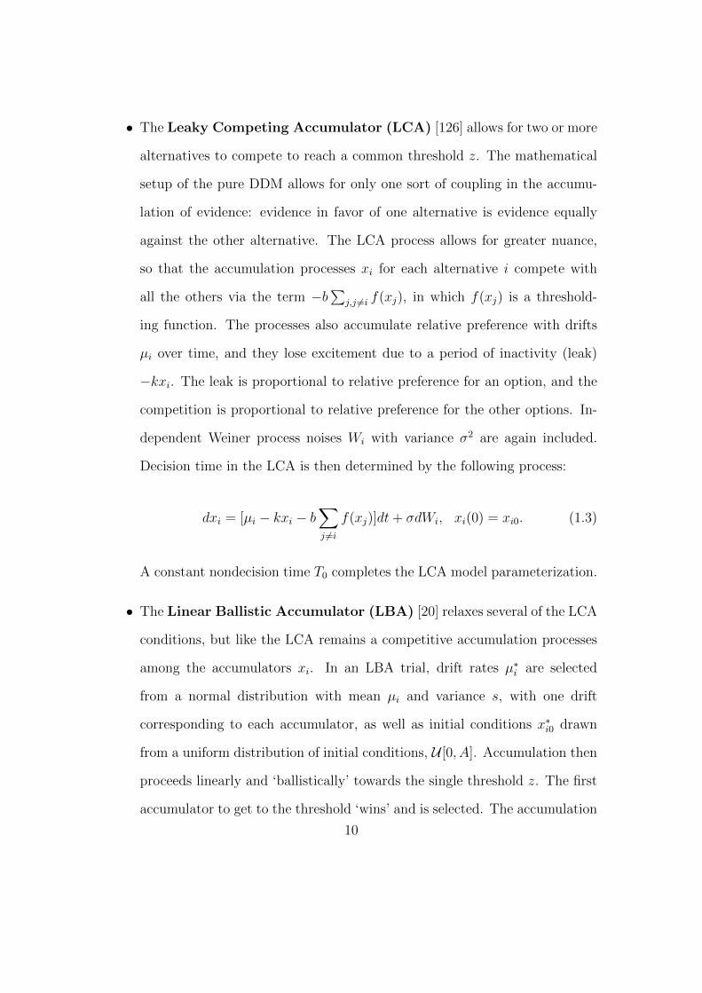
• The Leaky Competing Accumulator (LCA) [126] allows for two or more

alternatives to compete to reach a common threshold z. The mathematical

setup of the pure DDM allows for only one sort of coupling in the accumu-

lation of evidence: evidence in favor of one alternative is evidence equally

against the other alternative. The LCA process allows for greater nuance,

so that the accumulation processes xi for each alternative i compete with

all the others via the term −b∑j,j 6=i f(xj), in which f(xj) is a threshold-

ing function. The processes also accumulate relative preference with drifts

µi over time, and they lose excitement due to a period of inactivity (leak)

−kxi. The leak is proportional to relative preference for an option, and the

competition is proportional to relative preference for the other options. In-

dependent Weiner process noises Wi with variance σ2 are again included.

Decision time in the LCA is then determined by the following process:

dxi = [µi − kxi − b∑j 6=i

f(xj)]dt+ σdWi, xi(0) = xi0. (1.3)

A constant nondecision time T0 completes the LCA model parameterization.

• The Linear Ballistic Accumulator (LBA) [20] relaxes several of the LCA

conditions, but like the LCA remains a competitive accumulation processes

among the accumulators xi. In an LBA trial, drift rates µ∗i are selected

from a normal distribution with mean µi and variance s, with one drift

corresponding to each accumulator, as well as initial conditions x∗i0 drawn

from a uniform distribution of initial conditions, U [0, A]. Accumulation then

proceeds linearly and ‘ballistically’ towards the single threshold z. The first

accumulator to get to the threshold ‘wins’ and is selected. The accumulation

10

processes are then determined by the following equation:

xi(t) = x∗i0 + µ∗i t, (1.4)

where the first xi that reaches threshold is selected and the corresponding

time at which this happens is the decision time for the task. In a small

number of trials, all drift rates µ∗i will be negative and so a decision is never

made, consistent with a small portion of experimental tasks in which subjects

fail to respond. A constant nondecision time T0 completes the LBA model

parameterization.

Figure 1.2 illustrates key features of each of the models described above.

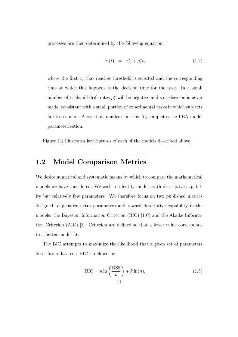
1.2 Model Comparison Metrics

We desire numerical and systematic means by which to compare the mathematical

models we have considered. We wish to identify models with descriptive capabil-

ity but relatively few parameters. We therefore focus on two published metrics

designed to penalize extra parameters and reward descriptive capability in the

models: the Bayesian Information Criterion (BIC) [107] and the Akaike Informa-

tion Criterion (AIC) [3]. Criterion are defined so that a lower value corresponds

to a better model fit.

The BIC attempts to maximize the likelihood that a given set of parameters

describes a data set. BIC is defined by

BIC = n ln

(RSS

n

)+ k ln(n), (1.5)

11

in which RSS is the residual sum of squares for the model predictions. The pa-

rameters n and k are the sample size or number of points the model is designed

to fit and the number of parameters in the model, respectively.

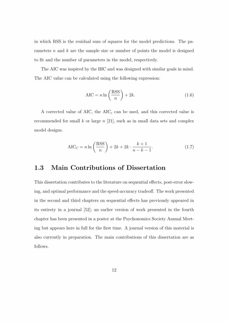
The AIC was inspired by the BIC and was designed with similar goals in mind.

The AIC value can be calculated using the following expression:

AIC = n ln

(RSS

n

)+ 2k. (1.6)

A corrected value of AIC, the AICc can be used, and this corrected value is

recommended for small k or large n [21], such as in small data sets and complex

model designs.

AICC = n ln

(RSS

n

)+ 2k + 2k · k + 1

n− k − 1. (1.7)

1.3 Main Contributions of Dissertation

This dissertation contributes to the literature on sequential effects, post-error slow-

ing, and optimal performance and the speed-accuracy tradeoff. The work presented

in the second and third chapters on sequential effects has previously appeared in

its entirety in a journal [52]; an earlier version of work presented in the fourth

chapter has been presented in a poster at the Psychonomics Society Annual Meet-

ing but appears here in full for the first time. A journal version of this material is

also currently in preparation. The main contributions of this dissertation are as

follows.

12

1. We developed a new model which accounts for both post-error slow-

ing and sequential effects. Our adapted DDM is based on a pure DDM

with systematic variation of the initial condition and thresholds, driven by

responses on previous trials.

2. We conducted an original experimental study showing that sequen-

tial effects vary with probability of alternations. We also showed that

our adapted DDM could account for these sequential variations in RT and

ER with the probability of alternations.

3. We identified key differences between the LBA and DDM accounts

of behavior in reward maximization tasks. In particular, we compared

fits to experimental data (kindly provided by Fuat Balci [6]) and analytical

predictions for the behavior of both high- and low-earning subjects. We

found that while both the DDM and LBA models could adequately predict

behavior in choice tasks, the two models gave very different explanations for

average subject behavior: the DDMs predicted that participants exercised

more caution as the tasks became easier, whereas the best-fit LBA predicted

that they exercised less caution.

To do this, we focused on the role of the caution parameter in a series of

neurally-plausible models. For the first two contributions, we adjusted caution

differently after correct and error trials. For the final contribution, we allowed

caution to be manipulated by overall preferences for relative speed or accuracy.

13

1.4 Outline of Dissertation

The structure of this dissertation is as follows. The next two chapters consider

sequential patterns in RT. The fourth chapter investigates the influence of reward

on overall RT and ER, and hence on the speed-accuracy tradeoff.

In Chapter 2, we consider sequential effects in simple, unbiased RT tasks. We

separately consider RTs for correct trials, error trials, and on average, as well as

the error rates. Comparing these data points with those predicted by prior model

fits to a data set, we find poor fits. We develop a new model, adapted from the

pure DDM, and we show that this model recreates sequential effects for error and

correct trials, whereas the other models do not.

In Chapter 3, we consider the results of an original experiment in which se-

quential effects are studied in response to biased random stimuli, for which either

repetition or alternation trials are more likely. Applying our model from the pre-

vious chapter, we again find that it accounts for trends in the data.

In Chapter 4, we compare the pure and extended DDM accounts of simple

choice behavior with the accounts of the LBA describing performance in reward

maximization tasks. We show that while each model can account for average sub-

ject behavior, and both DDMs can also account for the highest earning subjects,

the LBA accounts for behavior by predicting participants behave with less caution

in instances in which the DDM predicted that they used greater caution.

The final chapter details our conclusions and directions for future work.

14

Pure Drift Diffusion Model

Extended Drift Diffusion Model

Leaky Competing Accumulator Model

Linear Ballistic Accumulator Model

Correct threshold, +z

Correct threshold, +z

Error threshold, -z

Error threshold, -z

Single threshold, +z

Single threshold, +z

Drift μNoise σ

Initial condition x0

Initial condition from U[x

0-s

x/2,x

0+s

x/2]

Initial conditions x

i0

Drifts from N[μ,sμ]

Noise σ

Drifts μi

Noise σ

Leak -kxi

Competition -Σbf(xj)

Initial conditions from U[0,A]

Drifts from N[μi, s]

Single accumulator

Initial condition x0

Single accumulator

Single accumulator

Multiple accumulators

Multiple accumulators

Figure 1.2: Comparison of popular models of the decision making process: theDrift Diffusion Model (DDM), extended DDM, Leaky Competing AccumulatorModel, and Linear Ballistic Accumulator Model.

15

Chapter 2

Responses to Unbiased Random

Stimuli∗

Efforts to model and predict human behavior are informed by an understanding

of the dynamics of error rates (ERs) and reaction times (RTs) in simple tasks. In

particular, in two-alternative forced-choice (TAFC) tasks (e.g., [72, 73, 74, 96]) hu-

man participants are known to slow down after committing an error and generally

to exhibit RTs and ERs that systematically depend on prior stimulus sequences

[8, 25, 72, 102, 69, 130, 114, 113]. However, while much previous work has con-

sidered post-error slowing and sequential effects separately, we are not aware of

studies that explicitly account for interactions among these effects. In this chapter

we consider the effect of post-error slowing on sequential RT patterns in tasks in

which subjects are responding to unbiased random stimuli.

∗This chapter is presented with approximately 90% of the text and figures extracted verbatimfrom parts of [52]. Exceptions include minor textual changes throughout and extended detailsof the experimental setup, which are new.

16

Patterns in RTs for individual trials are well documented in the literature.

In particular, relative to their mean RTs on correct trials, subjects are known

to respond faster on error trials and more slowly immediately following errors

[89, 71, 70]. On average it has been shown that participants return to their mean

RT values within two trials after an error [91]. Various models of TAFC tasks

have accounted for this post-error slowing [96, 40]. In addition, RTs and ERs

are known to vary systematically with repeating (R, current stimulus is the same

as the previous stimulus) and alternating (A, present stimulus differs from the

previous stimulus) stimuli even when stimulus order is selected randomly and

each stimulus is equally likely [8, 71, 114]. Several other TAFC models account for

these sequential effects [28, 66, 46]. However, to our knowledge the mean RTs on

trials following specific sequences of stimuli have not been studied independently

for trials ending in an error, and deliberate post-error adjustments have not been

incorporated into models of sequential effects.

In this chapter, we study sequential patterns in ERs as well as in RTs for

error and correct responses independently in TAFC tasks in which stimuli are

equally probable with no bias towards either repetitions or alternations, focusing on

sequences of three trials. We reanalyze behavioral data from an equal-probability

experiment [28] with a relatively long response to stimulus interval (RSI, 800 ms).

In the following chapter, we will consider responses to stimuli with constant bias

towards repetitions or alternations.

To further study patterns in RT and ER we extend the pure drift diffusion

model (DDM) to account for sequential patterns. As noted in Chapter 1, Section

1.1, the pure DDM describes choice between two alternatives by representing the

noisy accumulation of the difference in evidence (logarithmic likelihood) from a

17

given initial condition to one of two decision thresholds. This process is known

to mimic aspects of neural integration [26, 50, 10, 49]. Adapting the DDM, we

propose two simple update mechanisms to vary the initial condition and thresholds

from trial to trial, depending on previous stimuli and response correctness. We

show how our adapted DDM can account for the observed trends in RT for correct

and error trials.

Related TAFC models frequently involve a variant of the leaky competing accu-

mulator (LCA) [126], featuring two coupled stochastic differential equations which

contain multiple parameters to account for leakage (decay of previous evidence)

and for the interaction between neural populations. LCA models have been shown

to capture sequential effects for equally-probable stimuli [28, 46]. For certain pa-

rameter ranges, it can be shown that the LCA, along with race, inhibition, and

other models, reduces to a DDM [10], and the DDM itself may be extended to

account for variability in the model parameters [97]. However, we are aware only

of modeling studies that predict both ERs and RTs for sequential effects [28, 46],

and these studies did not analyze patterns in error RTs, nor did they incorporate

post-error parameter adjustments into the analysis. Bayesian models of TAFC,

which can also be represented by DDMs for certain parameter ranges [75], have

also been used to model sequential effects [133, 132], but none of these models yet

accounts for patterns in errors.

Physiological evidence suggests sources of systematic changes in behavior from

trial to trial, providing some neurobiological basis for our proposed update mech-

anisms. An electroencephalogram (EEG) study has identified a SE pattern in the

P300 response [116], an event related potential signal which follows 300-600 ms

after unexpected, alternating, stimuli. The prefrontal cortex is also activated fol-

18

lowing an alternation after frequent repetitions, with greater activation following

a longer run of repetitions prior to the alternation [57]. In addition, the anterior

cingulate cortex (ACC) is known to show increased activity with increased conflict

in representation, or alternation of stimuli, and ACC activity has been linked to

cognitive control and post-error corrections and corresponding increase in RT [12].

Prior work has incorporated ACC conflict signals into models of sequential and

error effects [66].

This chapter is organized as follows. In Section 2, we describe the experimental

protocol, first reported in [28]. We then describe a diffusion model account of

participant behavior. In Section 3, we describe the experimental results and discuss

diffusion model fits to participant behavior. Finally, Section 4 contains further

discussion and our conclusions, and identifies directions for future experimental

and modeling work. Mathematical details are relegated to an Appendix.

2.1 Materials and methods

In this section, we describe the protocol followed for the experiment presented

in this chapter. We then describe a general model of decision making, which

accounts for choice behavior with two simple mechanistic adaptations to the pure

drift diffusion model (DDM). Finally, we describe a procedure for fitting the model

to match participant data in our adapted DDM.

2.1.1 Experiment 1: Unbiased random stimuli

In the experiment (reanalyzed from [28]), subjects participated in a classic two al-

ternative forced choice task. Seated in front of a computer screen, with their hands

19

on a keyboard, the subjects were presented with a series of stimuli in sequence.

After the subject identified the current stimulus with a keypress, the next stimulus

would then be presented after a short delay period. Stimulus probabilities were

equal and transition probabilities were held constant at 50%. As the details of the

experiment have been described in the literature previously, we outline them only

briefly here.

Six Princeton University undergraduates participated in a task over a single

session by identifying the upper or lowercase “o” character on the screen with the

appropriate keypress. The index finger was used to identify the uppercase letter,

and the middle finger to identify the lowercase letter. Each session consisted of 13

blocks of 120 trials each, and a response to stimulus interval (RSI) of 800 ms was

used. Participants received course credit in exchange for their participation in the

study: correct responses were not specifically rewarded, nor were errors penalized.

For additional details see [28]. No trials were omitted from our reanalysis.

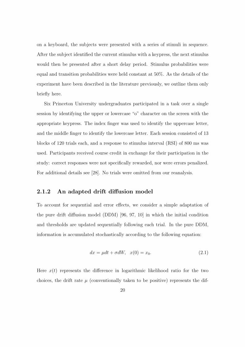
2.1.2 An adapted drift diffusion model

To account for sequential and error effects, we consider a simple adaptation of

the pure drift diffusion model (DDM) [96, 97, 10] in which the initial condition

and thresholds are updated sequentially following each trial. In the pure DDM,

information is accumulated stochastically according to the following equation:

dx = µdt+ σdW, x(0) = x0. (2.1)

Here x(t) represents the difference in logarithmic likelihood ratio for the two

choices, the drift rate µ (conventionally taken to be positive) represents the dif-

20

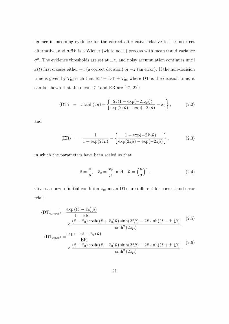
ference in incoming evidence for the correct alternative relative to the incorrect

alternative, and σdW is a Wiener (white noise) process with mean 0 and variance

σ2. The evidence thresholds are set at ±z, and noisy accumulation continues until

x(t) first crosses either +z (a correct decision) or −z (an error). If the non-decision

time is given by Tnd such that RT = DT + Tnd where DT is the decision time, it

can be shown that the mean DT and ER are [47, 22]:

〈DT〉 = z tanh(zµ) +

{2z(1− exp(−2x0µ))

exp(2zµ)− exp(−2zµ)− x0

}, (2.2)

and

〈ER〉 =1

1 + exp(2zµ)−{

1− exp(−2x0µ)

exp(2zµ)− exp(−2zµ)

}, (2.3)

in which the parameters have been scaled so that

z =z

µ, x0 =

x0

µ, and µ =

(µσ

)2

. (2.4)

Given a nonzero initial condition x0, mean DTs are different for correct and error

trials:

〈DTcorrect〉 =exp ((z − x0) µ)

1− ER

× (z − x0) cosh((z + x0)µ) sinh(2zµ)− 2z sinh((z − x0)µ)

sinh2 (2zµ),

(2.5)

〈DTerror〉 =exp (− (z + x0) µ)

ER

× (z + x0) cosh((z − x0)µ) sinh(2zµ)− 2z sinh((z + x0)µ)

sinh2 (2zµ).

(2.6)

21

See the Appendix for derivations of Eqs. (2.5-2.6).

The simplicity and analytical tractability of the DDM is a motivating factor

in our decision to use it as a basis for our study. We note that the DDM is much

simpler than the Leaky Competing Accumulator (LCA) Model [126], which has

been used in prior models of sequential effects [28, 66, 46]. LCA processes involve

two or more coupled nonlinear and stochastic differential equations (see Chapter

1, section 1.1 above). We shall compare predictions of the adapted DDM with

the LCA-based Cho [28], Jones [66], and Gao [46] models in Section 2.2, using the

data of Experiment 1.

Priming mechanism

As with other sequential effects models (e.g., [28, 66, 46]), parameters are updated

by a priming mechanism to reflect the stimulus history of repetitions and alterna-

tions and its influence on subject behavior. In the Cho, Jones, and Gao Models,

priming is implemented by small history-based changes to the drift parameter, µ.

In contrast, in our adapted DDM we update the initial conditions at trial n + 1

by setting

x0(n+ 1) = ±k(M(n)− 1

2

)± xoffset, (2.7)

in which n is the previous trial number, k > 0 is a scaling constant, and M(n)

serves as a dynamic memory of repetitions and updates at the start of each new

trial. M(n) is confined to the interval [0,1], so that M(n)− 12

ranges from −12

to 12.

A symmetry between R and A biases is then enforced: a positive value of M(n)− 12

corresponds to bias towards R trials and a negative M(n)− 12

corresponds to bias

22

towards A trials. Moreover, updates to M(n) are defined such that an increase

in bias towards R trials will correspond to a decrease in bias towards A trials,

and vice versa. Without loss of generality, we define our model terms such that

the positive direction for xoffset always corresponds to the correct response. The

normalized drift parameter µ must then always take a positive value, and the sign

of the offset bias xoffset and the scaling constant k will vary from trial to trial,

with positive coefficients selected if the current trial is a repetition of the previous

stimulus and negative coefficients if it is an alternation.

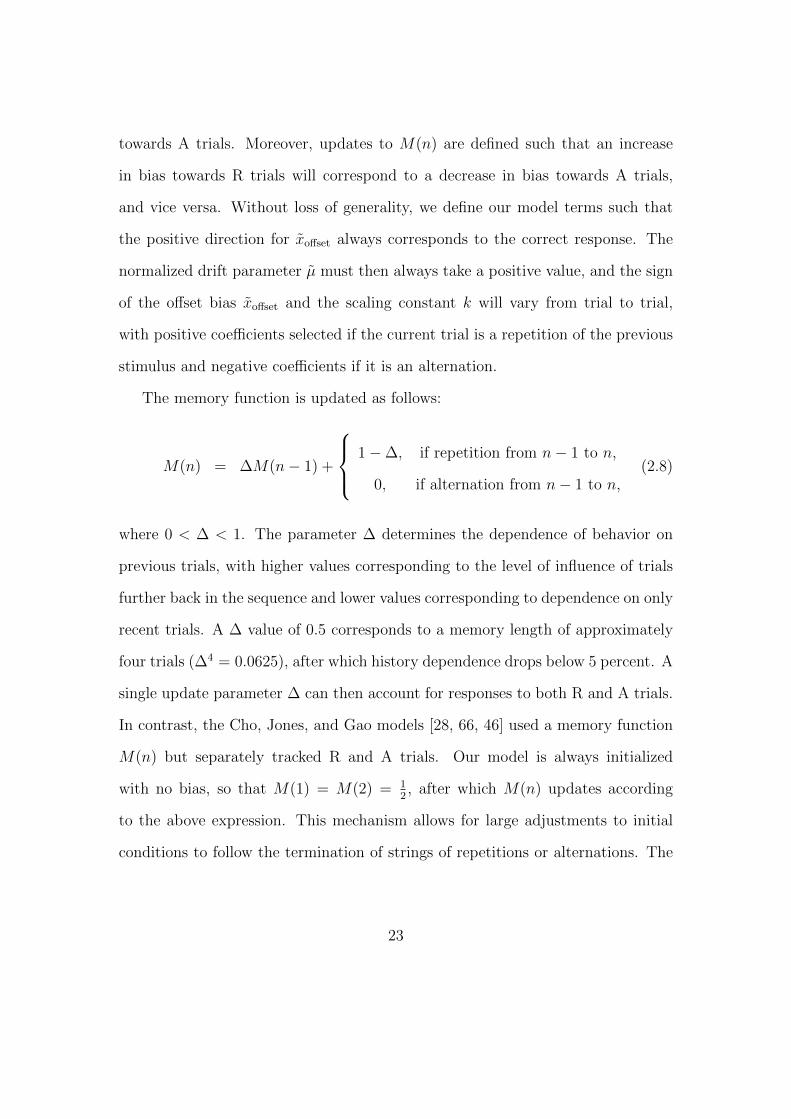
The memory function is updated as follows:

M(n) = ∆M(n− 1) +

1−∆, if repetition from n− 1 to n,

0, if alternation from n− 1 to n,(2.8)

where 0 < ∆ < 1. The parameter ∆ determines the dependence of behavior on

previous trials, with higher values corresponding to the level of influence of trials

further back in the sequence and lower values corresponding to dependence on only

recent trials. A ∆ value of 0.5 corresponds to a memory length of approximately

four trials (∆4 = 0.0625), after which history dependence drops below 5 percent. A

single update parameter ∆ can then account for responses to both R and A trials.

In contrast, the Cho, Jones, and Gao models [28, 66, 46] used a memory function

M(n) but separately tracked R and A trials. Our model is always initialized

with no bias, so that M(1) = M(2) = 12, after which M(n) updates according

to the above expression. This mechanism allows for large adjustments to initial

conditions to follow the termination of strings of repetitions or alternations. The

23

updating mechanism is similar to updates to biasing terms proposed in previous

work [28, 46], in which initial conditions and drift rates are updated.

Error-correcting mechanism

We also employ error-correction threshold modulation. Threshold modulation has

been studied in the context of several sequential choice tasks [10, 109]. In partic-

ular, models have used variable thresholds in describing optimal behavior, as well

as to account for variability in reaction time. Increased caution is attributed to a

higher threshold, which is understood to follow error commission. However, prior

models of sequential effects have not included threshold modulation.

In the adapted DDM, the thresholds are adjusted after every trial and con-

strained to remain symmetric at±z. After a correct trial, z is reduced by zdown > 0,

and after an error trial, increased by zup > 0:

z(n) = z(n− 1) +

−zdown, if correct at n− 1,

zup if error at n− 1.(2.9)

The range of z(n) is constrained so that the thresholds always have a magnitude

greater than or equal to the magnitude of the initial conditions, i.e., such that

z(n) ≥ k2

+ xoffset; z(n) is also constrained so that z(n) ≤ zmax. The thresholds

are initialized conservatively such that z(1) = zmax. If an update causes z(n) to

fall outside its bounds, z(n) is then set to the value of the nearest bound until the

next trial.

Sequential, error-correcting variations in the evidence thresholds z(n) can pro-

duce significant differences between reaction times for correct and error trials.

24

Trials with lower thresholds have higher ERs and faster RTs; thus, on average,

error trials are faster and correct trials slower. This effect is modulated by ad-

justments to the initial condition x0, which result in faster correct or incorrect

responses by biasing the system asymmetrically to start nearer one of the thresh-

olds. The memory function and initial condition and threshold updates remove z,

and add six parameters to the model: k, xoffset, ∆, zdown, zup, and zmax, in addition

to µ and Tnd, for a total of eight parameters.

2.1.3 Model simulation and data fitting procedure

Fitted model parameters were used to validate the adapted DDM against data from

Experiment 1. The data were sorted by sequence, RT, and ER. Model behavior

was computed for each parameter set and then sorted similarly. The model was

run using the same stimulus sequences that each participant had encountered.

Parameters were selected by attempting to minimize the sum of squared errors

between model prediction and participant data,

Err =N∑i=1

(ri,model − ri,data)2, (2.10)

in which the elements ri include unweighted overall mean RTs for each of the four

possible second-order sequences for R and A stimuli. We considered RR, AR, RA,

and AA (R followed by R, A followed by R, etc.) sequences for correct trials, for

error trials, and for trials overall, mean ERs for these sequences, as well as mean

RTs before error trials, on error trials, and after error trials. For the experiment

described in this chapter, r had N = 19 elements. Time was measured in units of

25

seconds and ERs in decimal fractions of trials, so that ranges of values for elements

of r were comparable.

The search for parameters was conducted using a Trust-Region-Reflective Opti-

mization (TRRO) algorithm [31, 32]. The function lsqnonlin in Matlab was used

with default options to search and select parameters that minimize Eq. (2.10).

For each parameter set and experimental condition, the model ran at least 5 times

through the stimulus sequence that each participant had encountered in a given

block of trials. (Thus, if a participant were to see big, then big, then small “o”

stimuli, the model was presented with those same stimuli in sequence big-big-small,

along with the stimuli preceding and following them, and these entire sequences

would be repeated for the model subject at least 5 times.) For each trial the prob-

ability of error was computed from Eq. (2.3) and from this number the correctness

or error of that trial was decided by biased coin flip. The expected correct or error

RT for the trial was then obtained from Eq. (2.5) or Eq. (2.6), and parameter

updates were implemented according to Eqs. (2.7-2.9). The individual trial results

were then sorted and averaged in the same manner as the experimental data, model

predictions were inserted into Eq. (2.10), and model parameters were updated by

the TRRO algorithm. This was repeated until the lsqnonlin convergence cri-

terion was met. The model was then simulated, with the converged paramter

values, being run 10 times on the stimulus sequences that each participant had

encountered, to produce the averaged model results displayed below.

Use of the analytical expressions of Eqs. (2.3-2.6) for expected ERs and RTs

substantially speeds up the fitting process, since direct numerical simulations of

Eq. (2.1) are avoided. The final parameter selections are listed in Table 1, and

26

the results and implications of the fitting process are considered in the results and

discussion sections of this chapter.

Table 2.1: DDM Parameterization for Experiment 1 of [28]

µ Tnd k x0,offset ∆ zdown zup zmax

38.1747 0.2626 0.0943 0.0051 0.6860 0.0058 0.0348 0.2857

2.2 Results

In order to better understand the relationship between sequential and error effects,

data from the experiment was sorted by stimulus sequence and response correctness

and compared with model predictions. We first note several trends from this

analysis in the data. We then validate our model fit by comparing it with the data

from Experiment 1.

In our analysis, we refer to RA and AR sequences as unexpected sequences, and

RR and AA sequences as expected sequences. The RT for an RA sequence is the

RT corresponding to the A trial, and for an AR sequence, the RT corresponding

to the R trial. We call an R line one which connects plotted data for RR and AR,

and an A line one which connects plotted data for RA and AA. We consider only

the two most recent trials in each sequence in our calculations, as the effects of

errors are known to persist only for a limited duration [89].

We consider sequential effects and error effects in data from Experiment 1 [28]

(referred to as Cho Data), in which R and A trials were equally likely, and as has

been customary, we initially average over all responses, correct and incorrect. We

first discuss overall sequential effects in RT and ER, as shown in Figure 2.1. As

27

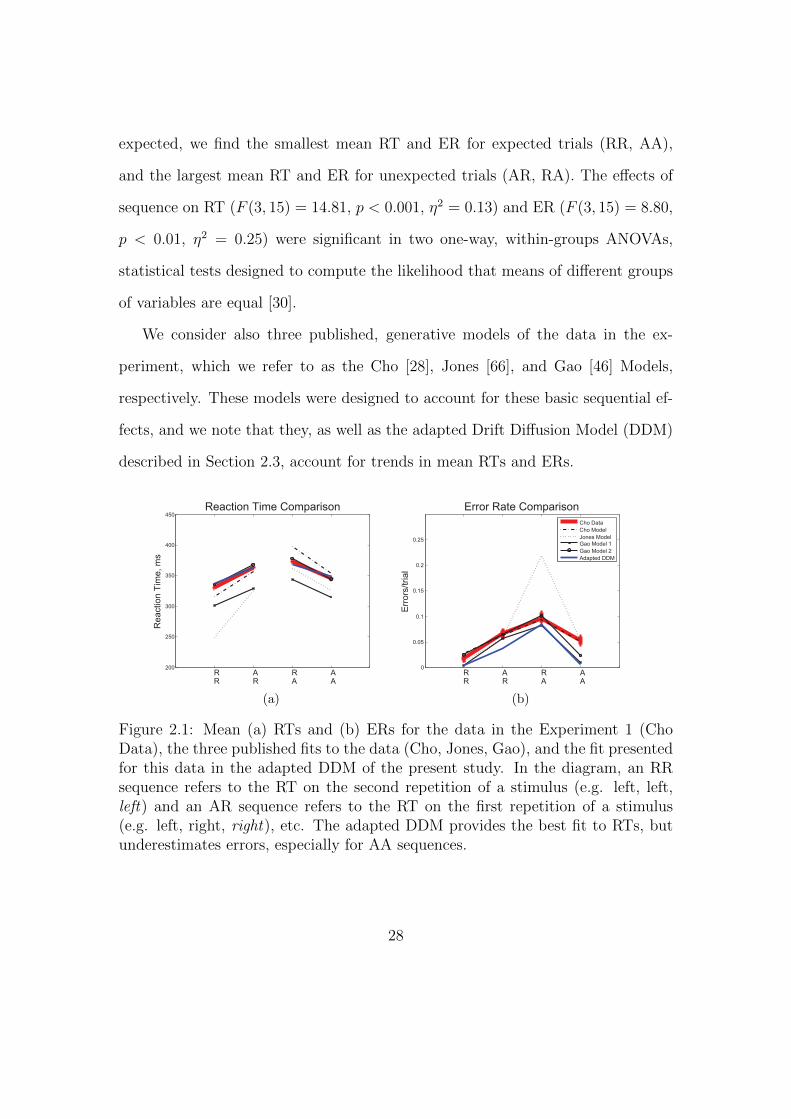
expected, we find the smallest mean RT and ER for expected trials (RR, AA),

and the largest mean RT and ER for unexpected trials (AR, RA). The effects of

sequence on RT (F (3, 15) = 14.81, p < 0.001, η2 = 0.13) and ER (F (3, 15) = 8.80,

p < 0.01, η2 = 0.25) were significant in two one-way, within-groups ANOVAs,

statistical tests designed to compute the likelihood that means of different groups

of variables are equal [30].

We consider also three published, generative models of the data in the ex-

periment, which we refer to as the Cho [28], Jones [66], and Gao [46] Models,

respectively. These models were designed to account for these basic sequential ef-

fects, and we note that they, as well as the adapted Drift Diffusion Model (DDM)

described in Section 2.3, account for trends in mean RTs and ERs.

200

250

300

350

400

450

RR

AR

RA

AA

Reaction Time Comparison

Reaction T

ime,

ms

(a)

0

0.05

0.1

0.15

0.2

0.25

RR

AR

RA

AA

Error Rate Comparison

Err

ors

/trial

Cho Data

Cho Model

Jones Model

Gao Model 1

Gao Model 2

Adapted DDM

(b)

Figure 2.1: Mean (a) RTs and (b) ERs for the data in the Experiment 1 (ChoData), the three published fits to the data (Cho, Jones, Gao), and the fit presentedfor this data in the adapted DDM of the present study. In the diagram, an RRsequence refers to the RT on the second repetition of a stimulus (e.g. left, left,left) and an AR sequence refers to the RT on the first repetition of a stimulus(e.g. left, right, right), etc. The adapted DDM provides the best fit to RTs, butunderestimates errors, especially for AA sequences.

28

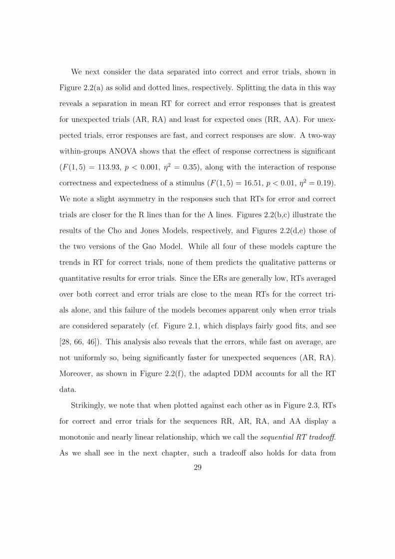
We next consider the data separated into correct and error trials, shown in

Figure 2.2(a) as solid and dotted lines, respectively. Splitting the data in this way

reveals a separation in mean RT for correct and error responses that is greatest

for unexpected trials (AR, RA) and least for expected ones (RR, AA). For unex-

pected trials, error responses are fast, and correct responses are slow. A two-way

within-groups ANOVA shows that the effect of response correctness is significant

(F (1, 5) = 113.93, p < 0.001, η2 = 0.35), along with the interaction of response

correctness and expectedness of a stimulus (F (1, 5) = 16.51, p < 0.01, η2 = 0.19).

We note a slight asymmetry in the responses such that RTs for error and correct

trials are closer for the R lines than for the A lines. Figures 2.2(b,c) illustrate the

results of the Cho and Jones Models, respectively, and Figures 2.2(d,e) those of

the two versions of the Gao Model. While all four of these models capture the

trends in RT for correct trials, none of them predicts the qualitative patterns or

quantitative results for error trials. Since the ERs are generally low, RTs averaged

over both correct and error trials are close to the mean RTs for the correct tri-

als alone, and this failure of the models becomes apparent only when error trials

are considered separately (cf. Figure 2.1, which displays fairly good fits, and see

[28, 66, 46]). This analysis also reveals that the errors, while fast on average, are

not uniformly so, being significantly faster for unexpected sequences (AR, RA).

Moreover, as shown in Figure 2.2(f), the adapted DDM accounts for all the RT

data.

Strikingly, we note that when plotted against each other as in Figure 2.3, RTs

for correct and error trials for the sequences RR, AR, RA, and AA display a

monotonic and nearly linear relationship, which we call the sequential RT tradeoff.

As we shall see in the next chapter, such a tradeoff also holds for data from

29

200

250

300

350

400

450

R RA R

R AA A

Cho D

ata

Reaction Time, ms

Corr

ect

Err

or

(a)

8

10

12

14

16

18

20

22

R RA R

R AA A

Cho M

odel

Reaction Time, ndu

(b)

10

12

14

16

18

20

22

R R

A R

R A

A A

Jones M

odel

Reaction Time, ndu

(c)

200

250

300

350

400

450

R RA R

R AA A

Gao M

odel 1

Reaction Time, ms

(d)

200

250

300

350

400

450

R RA R

R AA A

Gao M

odel 2

Reaction Time, ms

(e)

200

250

300

350

400

450

R RA R

R AA A

Adapte

d D

DM

Reaction Time, ms

(f)

Fig

ure

2.2:

Seq

uen

tial

effec

tsfr

omE

xp

erim

ent

1:(a

)dat

a,(b

)re

sult

sof

the

Cho

Model

[28]

,(c

)re

sult

sof

the

Jon

esM

odel

[66]

,(d

-e)

resu

lts

ofth

etw

oG

aoM

odel

s[4

6],

and

(f)

resu

lts

ofth

ead

apte

dD

DM

.T

he

Cho

and

Jon

esm

odel

spre

dic

ta

dim

ensi

onle

ssre

acti

onti

me,

whic

hw

egi

veher

ein

non

dim

ensi

onal

unit

s(n

du,

b,

c).

The

adap

ted

DD

Mca

ptu

res

the

slop

esof

the

Ran

dA

curv

esfo

rer

ror

and

corr

ect

tria

ls.

Inth

ese

figu

res,

the

corr

ectn

ess

orla

ckth

ereo

fof

agi

ven

tria

lco

rres

pon

ds

only

toth

attr

ial

itse

lf,

soa

left

-rig

ht-

left

sequen

ceis

tabula

ted

asco

rrec

tfo

rth

efinal

left

stim

ulu

sif

and

only

ifth

efinal

tria

lw

asid

enti

fied

corr

ectl

yas

ale

ftst

imulu

s.

30

Experiment 2 (Chapter 3). In Figure 2.3 we show the data from Experiment 1,

which is described in this chapter (R2 = 0.995, p < 0.01) and the adapted DDM,

and from a separate study by Jentzsch and Sommer [65] (R2 = 0.96, p < 0.05),

which both have strong correlations and high values of the correlation coefficient

R [30]. The area of the circles are proportional to the ERs for the given sequences.

We note that the smallest ERs correspond to sequences with relatively fast correct

responses and slow errors, while the high ERs occur with relatively fast errors and

slow correct responses. While the overall ordering of the sequences (RR, AR, RA,

AA) in the tradeoff differs between the two experimental studies, in both cases

the points corresponding to unexpected trials (AR, RA) lie at the upper left, and

those corresponding to expected trials (RR, AA) lie at the lower right.

230 240 250 260 270 280 290 300 310 320260

280

300

320

340

360

380

400

RR

AR

RA

AA

RR

AR

RA

AA

RT on Error Trial

RT

on C

orr

ect

Trial

RT Tradeoff in Previous Studies

Cho

Jentzsch

Adapted DDM

Figure 2.3: Sequential RT tradeoff for unbiased tasks: a slower RT for correcttrials corresponds to a faster RT for error trials for the sequences RR, AR, RA,and AA. The RT tradeoff for Experiment 1 is shown in red. Also shown, in blue:the RT tradeoff from a prior study by Jentzsch and Sommer [65]. Adapted DDMfits to data from Experiment 1 are shown in black. The areas of the circles areproportional to the ERs. The smallest and largest ERs are approximately 2% and10%, respectively.

31

The ordering of the tradeoffs is influenced by the nature of the task. However,

in each task we see that an increase in time to respond correctly (or a bias towards

the correct response) is correlated with a decrease in time to respond in error, and

vice versa. Our proposed biasing mechanism achieves a similar effect.

Finally, we consider the RTs before, during, and after an error in Experiment

1, as shown in Figure 2.4. Mean RTs for trials immediately following an error

are longer than both those for the error trial itself and for the trial immediately

before the error. A one-way within-groups ANOVA confirms that this effect on

RT is significant (F (2, 10) = 16.37, p < 0.001, η2 = 0.48). We again compare

the behavior with the adapted DDM and the three previous models. In the Cho

Model, the RT after an error is slower than the RT on the error trial but faster

than the trial immediately prior to the error. The Jones Model maintains the

trends in the data but parameter values are skewed so that the range of RTs is

larger. In the two Gao Models, mean RTs for trials immediately preceding and

following an error are faster than those on the error trial itself: opposite to the

data. The adapted DDM provides the best fit, with the RTs for error trials and

post-error trials closely matching the data, although it underestimates RTs on the

pre-error trial.

We compare the adapted DDM with the other models using the Akaike In-

formation Criterion (AIC, [1, 119]), corrected AIC (AICc, [59, 21]), and Bayesian

Information Criterion (BIC, [2, 112], which provide model fit comparisons that

account for the number of parameters included in each model, as described in

Chapter 1 Section 1.1. We also compute the square of the correlation coefficient

R [103], which quantifies the predictive relationship between between actual and

predicted values of experimental data. Scores for the different model fits are shown

32

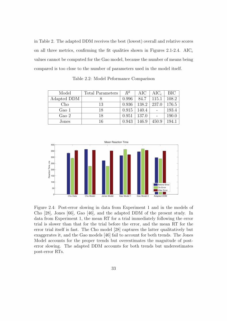
in Table 2. The adapted DDM receives the best (lowest) overall and relative scores

on all three metrics, confirming the fit qualities shown in Figures 2.1-2.4. AICc

values cannot be computed for the Gao model, because the number of means being

compared is too close to the number of parameters used in the model itself.

Table 2.2: Model Peformance Comparison

Model Total Parameters R2 AIC AICc BICAdapted DDM 8 0.996 84.7 115.1 108.2

Cho 13 0.936 138.2 237.0 176.5Gao 1 18 0.915 140.4 - 193.4Gao 2 18 0.951 137.0 - 190.0Jones 16 0.943 146.9 450.9 194.1

Cho Data Cho Model Jones Model Gao Model 1 Gao Model 2 Adapted DDM0

50

100

150

200

250

300

350

400

Reaction T

ime,

ms

Mean Reaction Time

Before Error

On Error

After Error

Figure 2.4: Post-error slowing in data from Experiment 1 and in the models ofCho [28], Jones [66], Gao [46], and the adapted DDM of the present study. Indata from Experiment 1, the mean RT for a trial immediately following the errortrial is slower than that for the trial before the error, and the mean RT for theerror trial itself is fast. The Cho model [28] captures the latter qualitatively butexaggerates it, and the Gao models [46] fail to account for both trends. The JonesModel accounts for the proper trends but overestimates the magnitude of post-error slowing. The adapted DDM accounts for both trends but underestimatespost-error RTs.

33

2.3 Discussion

In this chapter, we propose priming and error-correcting mechanisms to account

for sequential effects and post-error slowing, respectively. Each mechanism, on

its own, is commonplace in models of decision making. Indeed, various priming

mechanisms have been previously proposed to account for sequential effects [66, 28,

46]. Post-error slowing is also known to occur and exert a significant influence on

RT patterns [89, 90, 71]. The implementation of post-error slowing is understood

to be a simple one: in an accumulator model, the response thresholds can be raised

following an error to increase the necessary processing time before a decision is

reached [87, 88, 15, 61]. However, to the best of our knowledge, no prior model of

sequential effects has explicitly incorporated such an error-correcting mechanism

to also account for post-error slowing.

Our model is informed by previous work: the initial conditions are varied

according to a priming function similar to those in other models [28, 66, 46], and

the thresholds are raised after incorrect responses and lowered after correct ones

[109]. Variability in thresholds of drift diffusion processes during a trial can result

in fast errors [96]. Our implementation, however, is unique: we use both priming

and error-correcting mechanisms in the same model. In doing so, we can account

for many of the observed trends in behavior.

Our adaptation of the pure drift diffusion model has multiple advantages. The

pure DDM is analytically simple, and explicit expressions exist for both RT dis-

tributions and accuracy, and separate and closed form expressions for mean RTs

can be derived for correct and error responses, as shown in the Appendix of this

chapter. With nonzero initial conditions, the pure DDM can also account for

34

RT distributions for correct and error trials. Moreover, the priming and error-

correction mechanisms that we have proposed are conceptually straightforward.

With the error-correction mechanism, our model accounts for post-error slowing:

the RT for the trial which immediately follows an error trial is not only significantly

slower than the error trial but also slower than the RT for the trial immediately

preceding the error. We show that when thresholds are systematically adjusted

to account for error and correct responses and priming is implemented, sequential

patterns in error and correct response trial RTs emerge and are consistent with

participant behavior, as shown in Figure 2.4.

In the following chapter, we will see that the adapted DDM also accounts for

RT patterns when R and A trials are not equally likely. There we will discuss

in greater detail how the design of the adapted DDM allows us to capture this

behavior.

2.4 Appendix: Derivation of RTs for Correct

and Error Trials

In this section, we derive the mean reaction time for the drift diffusion model

(DDM) conditioned on hitting either the upper zu or lower −zl boundaries, and

for a general initial condition x0 ∈ (−zl, zu).

35

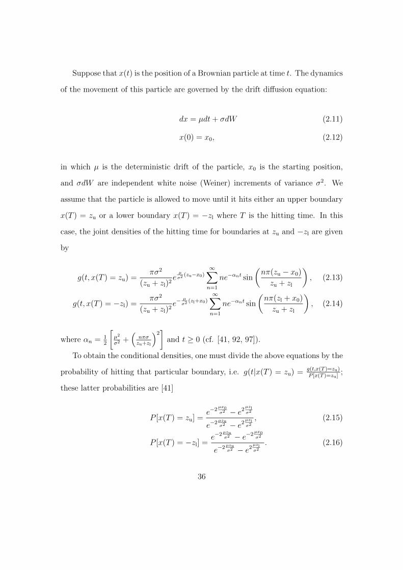
Suppose that x(t) is the position of a Brownian particle at time t. The dynamics

of the movement of this particle are governed by the drift diffusion equation:

dx = µdt+ σdW (2.11)

x(0) = x0, (2.12)

in which µ is the deterministic drift of the particle, x0 is the starting position,

and σdW are independent white noise (Weiner) increments of variance σ2. We

assume that the particle is allowed to move until it hits either an upper boundary

x(T ) = zu or a lower boundary x(T ) = −zl where T is the hitting time. In this

case, the joint densities of the hitting time for boundaries at zu and −zl are given

by

g(t, x(T ) = zu) =πσ2

(zu + zl)2eµ

σ2(zu−x0)

∞∑n=1

ne−αnt sin

(nπ(zu − x0)

zu + zl

), (2.13)

g(t, x(T ) = −zl) =πσ2

(zu + zl)2e−

µ

σ2(zl+x0)

∞∑n=1

ne−αnt sin

(nπ(zl + x0)

zu + zl

), (2.14)

where αn = 12

[µ2

σ2 +(

nπσzu+zl

)2]

and t ≥ 0 (cf. [41, 92, 97]).

To obtain the conditional densities, one must divide the above equations by the

probability of hitting that particular boundary, i.e. g(t|x(T ) = zu) = g(t,x(T )=zu)P [x(T )=zu]

;

these latter probabilities are [41]

P [x(T ) = zu] =e−2

µx0σ2 − e2

µzlσ2

e−2µzuσ2 − e2

µzlσ2

, (2.15)

P [x(T ) = −zl] =e−2µzu

σ2 − e−2µx0σ2

e−2µzuσ2 − e2

µzlσ2

. (2.16)

36

Thus, the mean reaction time conditioned on hitting the upper boundary is given

by

〈T 〉|zu =

∫ ∞0

tg(t|x(T ) = zu)dt

=1

P [x(T ) = zu]

πσ2

(zu + zl)2eµ

σ2(zu−x0)

∞∑n=1

n sin(nπ(zu−x0)zu+zl

)α2n

. (2.17)

Fortunately, a closed-form expression exists for the sum of the infinite series in the

previous equation [86, 125]:

∞∑n=1

n sin(ny)

(C2 +D2n2)2=

1

D2

[πy

4CD

cosh((π − y)C

D

)sinh

(π CD

) − π2

4CD

sinh(y CD

)sinh2

(π CD

)] . (2.18)

Setting C2 = µ2

2σ2 , D2 = (πσ)2

2(zu+zl)2and y = (zu − x0), after some algebra, we arrive

at a closed form for the mean decision time conditioned on hitting the upper

boundary:

〈T 〉|zu =1

P [x(T ) = zu]

1

µeµ(zu−x0)

σ2

×(zu − x0) cosh

(µ(zl+x0)

σ2

)sinh

(µ(zu+zl)

σ2

)− (zu + zl) sinh

(µ(zu−x0)

σ2

)sinh2

(µ(zu+zl)

σ2

) . (2.19)

In a similar fashion we obtain the mean decision time conditioned on hitting the

lower boundary:

〈T 〉|−zl =1

P [x(T ) = −zl]1

µe

−µ(zl+x0)

σ2

×(zl + x0) cosh

(µ(zu−x0)

σ2

)sinh

(µ(zu+zl)

σ2

)− (zu + zl) sinh

(µ(zl+x0)

σ2

)sinh2

(µ(zu+zl)

σ2

) . (2.20)

37

Chapter 3

Responses to Biased Random

Stimuli∗

Characteristic patterns in speed and accuracy following sequences of repetitions

and alternations are well documented only for tasks in which the stimuli are equally

likely. While overall trends in speed and accuracy have received significant atten-

tion [26, 97, 10, 110], for tasks in which the stimuli are not equally likely, such

sequential patterns in mean RT have not been considered. In this chapter, we con-

sider sequential effects in RT in tasks in which the order of stimulus presentation

is randomly biased towards either repetitions or alternations.

In a majority of TAFC studies, participants are either rewarded equally for

overall participation or they are rewarded for each correct response. However, sev-

eral studies (e.g. [33, 42]) have investigated tasks which reward correct responses

to one stimulus more highly than another and have shown that reward contin-

∗This chapter is presented with approximately 90% of the text and figures extracted verbatimfrom parts of [52]. Exceptions include details of the experimental setup, which are new.

38

gencies influence choice behavior. When reward probabilities or reward values are

unequal, participants are known to select the stimulus corresponding to the most

probable or most valuable reward more frequently [33, 42], and they may do so

almost optimally [42].

When stimuli are equally probable and correct responses are equally rewarded,

several stimulus sequence effects are known. For small (< 500 ms) response to

stimulus intervals (RSIs), the behavior typically illustrates automatic facilitation

(AF): mean RTs on the current trial are faster if the previous trial was a repetition,

regardless of whether the current trial is a repetition or an alternation. For slow

RSIs (≈1000 ms), mean RTs on the current trial after a series of alternations are

faster if the current trial is an alternation and slower if the current trial is an

repetition [8, 72, 69]. This effect is called strategic expectancy (SE), suggesting

a relationship between a participant’s expectations and his or her reaction time.

Moreover, a transition occurs from AF to SE as RSI increases [113, 65] and can be

illustrated graphically [4]. Prior to the present work, it was unknown whether such

a transition from AF to SE could also occur for a constant RSI with increasing

probability of alternations, or, more generally, how sequential effects carry over

from equally-probable to biased stimuli.

In this chapter, we study sequential patterns in ERs as well as in RTs for error

and correct responses independently in TAFC tasks in which stimuli are equally

probable or strongly biased towards repetitions or alternations, focusing on se-

quences of three trials. Stimulus sequences can be biased by specifying stimulus

probabilites (state orientation) or by specifying transition probabilities between

states (transition orientation), and it is known that these processes produce dis-

tinct response patterns in RT [19]. Since we are interested in sequential effects and

39

expectancy, we generate stimuli by a first-order Markov process with unequal (as

well as equal) transition probabilities (see Figure 3.1): The biased case sets the

probability of an alternation (PA) to be unequal to the probability of a repetition

(1 − PA). Transition probabilities PA and 1 − PA are held fixed over blocks of

trials, and we use relatively long RSIs (800 ms and 1,000 ms mean), for which SE

is most apparent. In this chapter, we collect and analyze a new data set with PA

set to 10%, 50%, and 90%. We find significant transition probability effects on

RTs for error and correct responses and on ERs.

An understanding of the relationship between error correction and sequential

biasing mechanisms may allow us to further differentiate between corresponding

physiological processes. Such an understanding could have broad implications.

Indeed, recent work suggests that the same mechanisms that account for sequential

effects also account for sequence learning [115]: a general mechanism may therefore

lend insight into sequence learning [113, 84, 85, 44], including linguistic processes.

Further, better understanding of the mechanisms behind simple discrimination

tasks may also allow for improved prediction and prevention of errors.

This chapter is organized as follows. In Section 2, we describe Experiment 2.

We then apply the diffusion model account of participant behavior developed in

Chapter 2, Section 2.1.2 to describe the behavior of human subjects in this task.

In Section 3, we describe the experimental results and discuss diffusion model fits

to participant behavior. Finally, Section 4 contains further discussion and our

conclusions, and identifies directions for future experimental and modeling work.

40

Stim

1

Stim

2

PA

PA

1-PA

1-PA

Figure 3.1: Stimulus order is generated by a transition-oriented Markov process.Given current stimulus 1, the next stimulus will be stimulus 2 (an alternation)with probability PA and stimulus 1 (a repetition) with probability 1− PA.

3.1 Materials and methods

In this section, we describe the protocol followed for Experiment 2. We then

describe the adapted DDM model fits, performed as in Chapter 2, Section 2.1.3,

and we compare the resulting parameters with those obtained in Chapter 2. We

also provide an interpretation of the fitted parameter values.

3.1.1 Experiment 2: Biased Random Stimuli

In this experiment stimulus transition probabilities were varied from block to block,

so that in a given block a participant would have a constant high, medium, or low

probability of alternations. That is, given the current stimulus 1, a participant

would next see stimulus 2 with probability PA and the same stimulus 1 again with

probability 1 − PA, with the sequence of stimuli being drawn from a transition-

oriented Markov process, with PA fixed during each block, as shown in Figure

3.1.

41

Participants

Sixteen adults (6 males) participated in exchange for a standard payment of $12

per session of 9 blocks. Participants were recruited from the Princeton University

community via announcements posted online and on campus. The experiment was

approved by the Institutional Review Panel for Human Subjects of Princeton Uni-

versity, and all participants provided their informed consent prior to participation.

Stimuli

Participants performed an RT version of a motion discrimination task. The visual

stimulus consisted of a black screen showing a cloud of white moving dots with

a red, stationary fixation dot at its center. The red dot had size 0.30 degrees

visual angle, and the white dots had size 0.15 degrees each and moved within a

circle of diameter 10 degrees at a speed of 7 degrees/second and a density of 20

dots/degree2. On each trial 90 percent of the white dots would move coherently in

a given, “correct” direction, and the remaining white dots would move randomly.

The high coherence of motion was selected to ensure that some processing was

necessary but that the difficulty of the task would remain low, consistent with

other studies of sequential effects. A decision could be indicated with a left or

right keypress at any point after dots appeared on the screen. Responses were

collected via the standard Macintosh computer keyboard, with the ‘Z’ key used

to indicate leftward motion and the ‘M’ key used to indicate rightward motion.

The experiment was performed on a Macintosh computer using the Psychophysics

Toolbox extension [14].

42

Procedure

The participants were instructed to fixate upon the red dot and then determine the

direction of the moving dots. They were also instructed to complete the session

as quickly and as accurately as possible. Each participant completed 1 session of

approximately 60 minutes duration.

Each session consisted of 9 blocks of 200 trials, in each of which PA remained

fixed at 10%, 50%, or 90% (3 blocks for each condition). The order of the blocks

was constrained to follow a Latin Square design. Participants were allowed a short

break between blocks. To minimize anticipatory responding, response to stimulus

intervals were drawn from a gamma distribution with a mean of 1 second for each

trial, following the convention set in previous sequential RT tasks [89, 109, 19, 6].

Outlier RTs (less than 100 ms or greater than 900 ms, comprising less than 1.5%

of the data) were not included in the analysis. We note that only the outlier was

removed from the RT and error analysis; it was included in sorting RR, AR, RA,

and AA sequences, since it precedes a trial that is included in the analysis. One

participant failed to follow instructions and the corresponding data were omitted

from the analysis.

During each block in the session, the subjects received the following feedback.

Correct responses were denoted with a short beep sound, and error and prema-

ture, anticipatory responses were denoted with a buzz sound. In addition, on

every fifth trial, the number of correct responses provided in that block so far was

briefly flashed across the screen. This was the only feedback that was provided.

Participants were seated at a viewing distance of approximately 60 cm from the

43

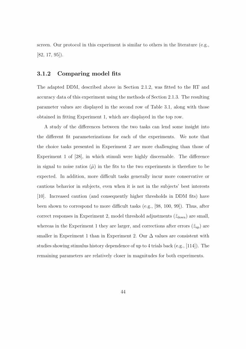
screen. Our protocol in this experiment is similar to others in the literature (e.g.,

[82, 17, 95]).

3.1.2 Comparing model fits

The adapted DDM, described above in Section 2.1.2, was fitted to the RT and

accuracy data of this experiment using the methods of Section 2.1.3. The resulting

parameter values are displayed in the second row of Table 3.1, along with those

obtained in fitting Experiment 1, which are displayed in the top row.

A study of the differences between the two tasks can lend some insight into

the different fit parameterizations for each of the experiments. We note that

the choice tasks presented in Experiment 2 are more challenging than those of

Experiment 1 of [28], in which stimuli were highly discernable. The difference

in signal to noise ratios (µ) in the fits to the two experiments is therefore to be

expected. In addition, more difficult tasks generally incur more conservative or

cautious behavior in subjects, even when it is not in the subjects’ best interests

[10]. Increased caution (and consequently higher thresholds in DDM fits) have

been shown to correspond to more difficult tasks (e.g., [98, 100, 99]). Thus, after

correct responses in Experiment 2, model threshold adjustments (zdown) are small,

whereas in the Experiment 1 they are larger, and corrections after errors (zup) are

smaller in Experiment 1 than in Experiment 2. Our ∆ values are consistent with

studies showing stimulus history dependence of up to 4 trials back (e.g., [114]). The

remaining parameters are relatively closer in magnitudes for both experiments.

44

Table 3.1: Comparison of DDM Parameterizations

µ Tnd k x0,offset ∆ zdown zup zmax

Experiment 1 38.1747 0.2626 0.0943 0.0051 0.6860 0.0058 0.0348 0.2857Experiment 2 19.3312 0.3359 0.1181 0.0034 0.6882 0.0034 0.1635 0.2062

3.2 Results

In order to better understand the relationship between sequential effects and error

effects, data from Experiment 2 was sorted by stimulus sequence and response

correctness and compared with model predictions as described in the previous

chapter. We then analyze this data and ask how error and sequential effects are

influenced by the relative frequencies of repetition (R) and alternation (A) trials.

At the same time, we validate our model fits by comparing them with the data

from Experiment 2.

In our discussion, we again refer to RA and AR sequences as unexpected se-

quences, and RR and AA sequences as expected sequences. The RT for an RA

sequence is the RT corresponding to the A trial, and for an AR sequence, the RT

corresponding to the R trial. As in Chapter 2, we call an R line one which con-

nects plotted data for RR and AR, and an A line one which connects plotted data

for RA and AA. We consider only the two most recent trials in each sequence in

our calculations, because the effects of errors are known to have a limited duration

[89]. We note also that for the strongly biased stimuli (PA = 10%, 90%), longer

sequences of A’s, respectively R’s, occur too rarely to yield sufficient data.

We now consider the role that alternation frequency plays in sequential and

error effects. We first address overall trends in RT and ER, as shown in Figures

45

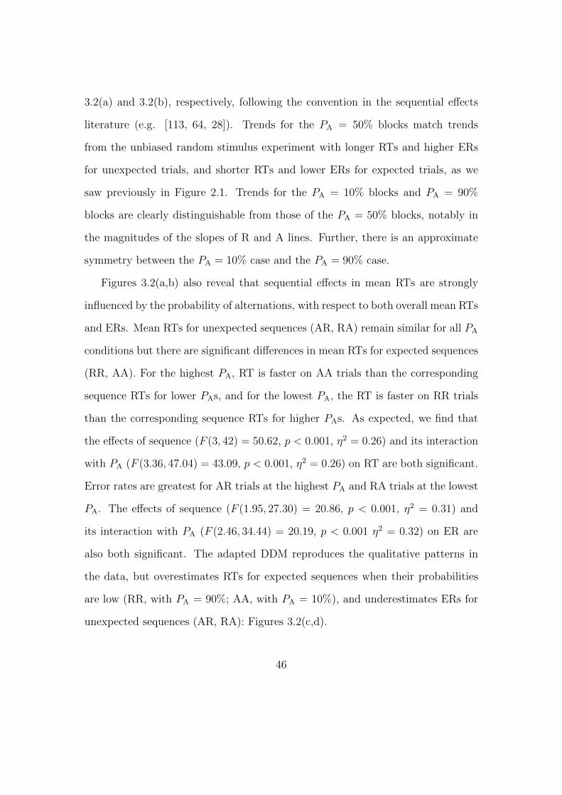
3.2(a) and 3.2(b), respectively, following the convention in the sequential effects

literature (e.g. [113, 64, 28]). Trends for the PA = 50% blocks match trends

from the unbiased random stimulus experiment with longer RTs and higher ERs

for unexpected trials, and shorter RTs and lower ERs for expected trials, as we

saw previously in Figure 2.1. Trends for the PA = 10% blocks and PA = 90%

blocks are clearly distinguishable from those of the PA = 50% blocks, notably in

the magnitudes of the slopes of R and A lines. Further, there is an approximate

symmetry between the PA = 10% case and the PA = 90% case.

Figures 3.2(a,b) also reveal that sequential effects in mean RTs are strongly

influenced by the probability of alternations, with respect to both overall mean RTs

and ERs. Mean RTs for unexpected sequences (AR, RA) remain similar for all PA

conditions but there are significant differences in mean RTs for expected sequences

(RR, AA). For the highest PA, RT is faster on AA trials than the corresponding

sequence RTs for lower PAs, and for the lowest PA, the RT is faster on RR trials

than the corresponding sequence RTs for higher PAs. As expected, we find that

the effects of sequence (F (3, 42) = 50.62, p < 0.001, η2 = 0.26) and its interaction

with PA (F (3.36, 47.04) = 43.09, p < 0.001, η2 = 0.26) on RT are both significant.

Error rates are greatest for AR trials at the highest PA and RA trials at the lowest

PA. The effects of sequence (F (1.95, 27.30) = 20.86, p < 0.001, η2 = 0.31) and

its interaction with PA (F (2.46, 34.44) = 20.19, p < 0.001 η2 = 0.32) on ER are

also both significant. The adapted DDM reproduces the qualitative patterns in

the data, but overestimates RTs for expected sequences when their probabilities

are low (RR, with PA = 90%; AA, with PA = 10%), and underestimates ERs for

unexpected sequences (AR, RA): Figures 3.2(c,d).

46

300

350

400

450

500

550

RR

AR

RA

AA

Reaction Time (Data)R

eaction T

ime,

ms

PA = 10

PA = 50

PA = 90

(a)

0

0.05

0.1

0.15

0.2

0.25

RR

AR

RA

AA

Error Rate (Data)

Err

ors

/trial

PA = 10

PA = 50

PA = 90

(b)

300

350

400

450

500

550

RR

AR

RA

AA

Reaction Time (Model)

Rea

ctio

n T

ime,

ms

PA = 10

PA = 50

PA = 90

(c)

0

0.05

0.1

0.15

0.2

0.25

RR

AR

RA

AA

Error Rate (Model)

Err

ors/

tria

l

P

A = 10

PA = 50

PA = 90

(d)

Figure 3.2: Mean (a) RTs and (b) ERs for the three values of PA in the biasedrandom stimulus experiment, averaged over correct and error trials. The influenceof PA is most apparent in the mean RT plot on expected trials (RR, AA) and inthe mean ER on unexpected trials (AR, RA). Model fits for (c) RTs and (d) ERsre-create behavioral trends in RTs and ERs but overestimate RTs for expectedtrials (RR, AA). The error bars in plots (a) and (b) represent the standard errorof the mean, and in (c) and (d) the average value of standard error of the meanover 10 simulation runs (see Chapter 2, especially Section 2.1.3, for details).

We also found that the overall sequential effects are influenced by the proba-

bility of alternations. The relationship between the time to respond to sequences

ending in R versus A on the final sequence is known to indicate relative preference

for R or A trials [4]. Prior work has shown that preference for A trials varies with

47

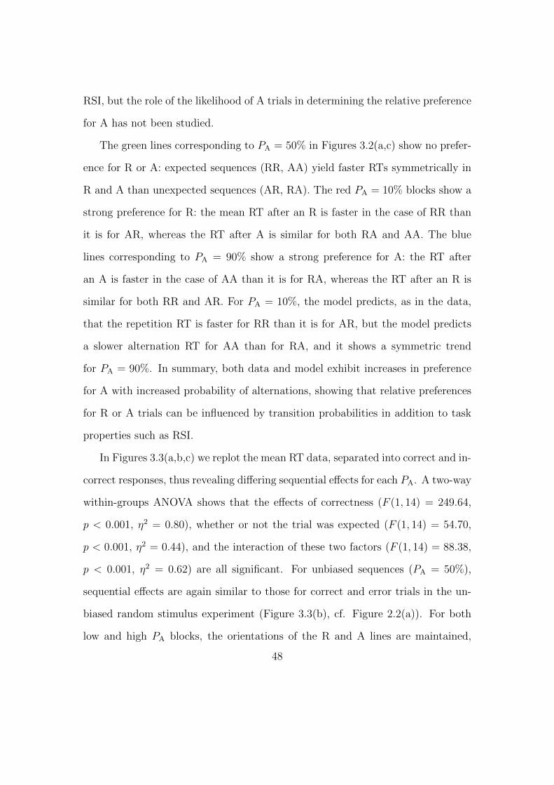
RSI, but the role of the likelihood of A trials in determining the relative preference

for A has not been studied.

The green lines corresponding to PA = 50% in Figures 3.2(a,c) show no prefer-

ence for R or A: expected sequences (RR, AA) yield faster RTs symmetrically in

R and A than unexpected sequences (AR, RA). The red PA = 10% blocks show a

strong preference for R: the mean RT after an R is faster in the case of RR than

it is for AR, whereas the RT after A is similar for both RA and AA. The blue

lines corresponding to PA = 90% show a strong preference for A: the RT after

an A is faster in the case of AA than it is for RA, whereas the RT after an R is

similar for both RR and AR. For PA = 10%, the model predicts, as in the data,

that the repetition RT is faster for RR than it is for AR, but the model predicts

a slower alternation RT for AA than for RA, and it shows a symmetric trend

for PA = 90%. In summary, both data and model exhibit increases in preference

for A with increased probability of alternations, showing that relative preferences

for R or A trials can be influenced by transition probabilities in addition to task

properties such as RSI.

In Figures 3.3(a,b,c) we replot the mean RT data, separated into correct and in-

correct responses, thus revealing differing sequential effects for each PA. A two-way

within-groups ANOVA shows that the effects of correctness (F (1, 14) = 249.64,

p < 0.001, η2 = 0.80), whether or not the trial was expected (F (1, 14) = 54.70,

p < 0.001, η2 = 0.44), and the interaction of these two factors (F (1, 14) = 88.38,

p < 0.001, η2 = 0.62) are all significant. For unbiased sequences (PA = 50%),

sequential effects are again similar to those for correct and error trials in the un-

biased random stimulus experiment (Figure 3.3(b), cf. Figure 2.2(a)). For both

low and high PA blocks, the orientations of the R and A lines are maintained,

48

300

350

400

450

500

550

R RA R

R AA A

PA =

10

Reaction Time, ms

Corr

ect

Err

or

(a)

300

350

400

450

500

550

R R

A R

R A

A A

PA =

50

Corr

ect

Err

or

(b)

300

350

400

450

500

550

R R

A R

R A

A A

PA =

90

Corr

ect

Err

or

(c)

300

350

400

450

500

550

R RA R

R AA A

PA =

10

Reaction Time, ms

C

orre

ctE

rror

(d)

300

350

400

450

500

550

R RA R

R AA A

PA =

50

C

orre

ctE

rror

(e)

300

350

400

450

500

550

R RA R

R AA A

PA =

90

C

orre

ctE

rror

(f)

Fig

ure

3.3:

(a-c

)R

Tdat

afo

rer

ror

and

corr

ect

tria

lsin

Exp

erim

ent

2co

mpar

edw

ith

the

adap

ted

DD

M(d

-f).

The

slop

esof

the

Ran

dA

lines

are

reve

rsed

for

corr

ect

and

inco

rrec

tre

spon

ses.

Err

ortr

ials

incu

rfa

ster

resp

onse

son

unex

pec

ted

tria

ls(R

A,A

R)

than

onex

pec

ted

tria

ls(R

R,A

A);

this

tren

dis

reve

rsed

for

corr

ect

resp

onse

s.F

orlo

wP

A,

the

Rlines

over

lap,

and

for

hig

hP

A,

the

Alines

over

lap,

resu

ltin

gin

anap

pro

xim

ate

reflec

tion

alsy

mm

etry

bet

wee

ndat

afo

rth

ehig

han

dlo

wP

Ablo

cks,

soth

atin

som

eca

ses

the

mea

nti

me

for

aner

ror

tria

lis

slow

erth

anfo

ra

corr

ect

tria

l.T

he

erro

rbar

sin

plo

ts(a

-c)

repre

sent

the

stan

dar

der

ror

ofth

em

ean,

and

in(d

-f)

the

aver

age

valu

eof

stan

dar

der

ror

ofth

em

ean

over

10si

mula

tion

runs

(see

Sec

tion

2.1.

3fo

rdet

ails

).

49

with correct R lines sloping upwards from RR to AR and correct A lines sloping

down from RA to AA. For PA = 50%, the slopes of the R and A lines for incorrect

responses are nearly opposite the slopes of the R and A lines for correct responses.

In contrast, for PA = 10% blocks, the R lines cross and the A lines are further

apart than in the PA = 50% blocks. For PA = 90% blocks, we see a mirrored

trend, in which the A lines cross and the R lines are further apart than in the PA

= 50% block. We also note a striking asymmetry for the biased stimuli: for PA

= 10% R lines are, on average, closer together than A lines, and for PA = 90%

this relationship is mirrored, so that A lines are closer than R lines. However, the

mirroring is not perfect: the degree of overlap in R lines is greater for PA = 10%

than the corresponding overlap in A lines for PA = 90%.

The trends in correct and error trial RTs, including the crossover of the R and A

lines, are generally captured by the adapted DDM, as shown in Figures 3.3(d,e,f).

However, the steepness of slope of the R (respectively A) lines are underestimated

for correct trials for PA = 90% (10%), due to overestimation of the RR (AA) RTs.

Next, we note that the sequential RT tradeoff between correct and error re-

sponses is also observed in Experiment 2, as shown in Figure 3.4(a). As in Figure

2.3, the areas of the circles are proportional to the corresponding ERs. The re-

lationship between RTs for correct and error trials for each of the sequences RR,

AR, RA, and AA is monotone (and nearly linear) for all points shown in the fig-

ure (R2 = 0.75, p < 0.001), and this correlation is also captured by our model

(R2 = 0.74, p < 0.001): Figure 3.4(b). The sequences with the largest ER have

relatively fast RTs for errors and relatively slow RTs for correct trials. Note,

however, that data for individual PAs of 10%, 50%, and 90% is not as strongly

50

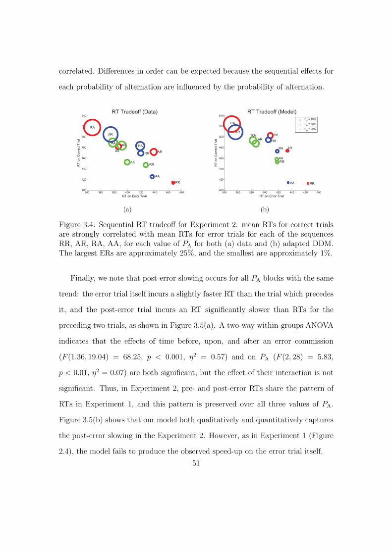
correlated. Differences in order can be expected because the sequential effects for

each probability of alternation are influenced by the probability of alternation.

340 360 380 400 420 440 460 480400

420

440

460

480

500

520

540

RT on Error Trial

RT

on C

orr

ect

Trial

RT Tradeoff (Data)

RR

AR

RA

AA

RR

ARRA

AA

RR

AR

RA

AA

(a)

340 360 380 400 420 440 460 480400

420

440

460

480

500

520

540

RT on Error Trial

RT

on C

orr

ect

Trial

RT Tradeoff (Model)

RR

AR

RA

AA

RR

AR

RA

AA

RR

AR

RA

AA

PA = 10%

PA = 50%

PA = 90%

(b)

Figure 3.4: Sequential RT tradeoff for Experiment 2: mean RTs for correct trialsare strongly correlated with mean RTs for error trials for each of the sequencesRR, AR, RA, AA, for each value of PA for both (a) data and (b) adapted DDM.The largest ERs are approximately 25%, and the smallest are approximately 1%.

Finally, we note that post-error slowing occurs for all PA blocks with the same

trend: the error trial itself incurs a slightly faster RT than the trial which precedes

it, and the post-error trial incurs an RT significantly slower than RTs for the

preceding two trials, as shown in Figure 3.5(a). A two-way within-groups ANOVA

indicates that the effects of time before, upon, and after an error commission

(F (1.36, 19.04) = 68.25, p < 0.001, η2 = 0.57) and on PA (F (2, 28) = 5.83,

p < 0.01, η2 = 0.07) are both significant, but the effect of their interaction is not

significant. Thus, in Experiment 2, pre- and post-error RTs share the pattern of

RTs in Experiment 1, and this pattern is preserved over all three values of PA.

Figure 3.5(b) shows that our model both qualitatively and quantitatively captures

the post-error slowing in the Experiment 2. However, as in Experiment 1 (Figure

2.4), the model fails to produce the observed speed-up on the error trial itself.

51

10 50 900

100

200

300

400

500

600

PA

Reaction T

ime,

ms

Post−Error Slowing (Data)

Before Error

On Error

After Error

(a)

10 50 900

100

200

300

400

500

600

PA

Rea

ctio

n T

ime,

ms

Post−Error Slowing (Model)

Before ErrorOn ErrorAfter Error

(b)

Figure 3.5: (a) Post-error slowing in data for the Experiment 2 is independent ofPA. (b) The model fit also predicts post-error slowing but does not fully accountfor pre-error speeding. The error bars in plot (a) represent the standard errorof the mean, and in (b) the average value of standard error of the mean over 10simulation runs (see Chapter 2 for details).

3.3 Discussion

Our adapted DDM predicts the characteristic trends in mean RTs for sequences

of both unbiased and biased random stimuli. We show experimentally and for

the first time that unexpected trials (AR or RA) result in relatively slow correct

responses and fast errors, whereas expected trials (RR or AA) result in relatively

fast correct responses and slow errors, as shown in Figure 3.3 (c.f. 2.2). Our model

captures aspects of this behavior with the incorporation of post-error adjustments

to the model thresholds: priming accounts for the sequential patterns in RT for

correct trials, and error-correction accounts for the patterns in RT for the error

trials.

The relationship between RTs for correct and error trials is central to our

model: biasing the initial conditions towards expected sequences automatically

52

biases them against unexpected sequences. Subjects biased against an unexpected

stimulus will then respond to it slowly if they are to respond correctly, and rapidly

if they are to respond in error. In contrast, in previous work [28, 66, 46], the biasing

was instead applied to sensitivity to stimulus, so that the relationship between RT

for error and correct trials was less direct. Moreover, when biasing is coupled with

explicit post-error adjustments, further nuances in the relationship between mean

time to respond correctly versus in error may be realized.

Significantly, we also identify a sequential RT tradeoff, in which the correlation

between the mean RTs for error and correct trials for each of the sequences (RR,

AR, RA, AA) is quite strong: a faster RT on an error response corresponds to a

slower RT on a correct response. The correlation between mean RTs for correct

and error trials is captured by our model, as shown in Figures 2.3 and 3.4.

The second experiment also shows that sequential effects in mean RTs overall,

as well as in mean RTs for correct and error trials, are significantly influenced by

the probability of alternations. Our data reveals remarkable near-mirror-symmetry

between RT patterns for alternations when the probability of alternations is low

and repetitions when the probability of alternations is high: incorrect responses

are fast and correct responses are significantly slower. Sequential effects in ER

also vary with the probability of alternations. Figures 3.2 and 3.3 show that our

model captures this near-symmetry.

Moreover, we have shown, both in our data and in our model, that an increase

in the likelihood of alternations corresponds to an increase in relative preference

for alternations. This can be inferred from the RT versus sequence plots in Figure

3.2(a). The change in alternation preference with changing likelihood of alterna-

53

tions suggests that choice behavior can be informed and even manipulated by the

probabilistic structure of the environment.

The sequential effects in RT and ER for various probabilities of alternation

are of particular interest due to their relevance to prior physiological and imag-

ing studies. In particular, previous work has shown that the anterior cingulate

cortex (ACC) is sensitive to alternations in a sequence of stimuli and identified

corresponding neural signals (e.g., [12]). Prior models of sequential effects, such

as those of Jones et al. [66] and Gao et al. [46] have included a “conflict” signal

modulated by activity in the ACC, and increasing in strength with frequent alter-

nations. However, the near symmetry of behavior at high and low probabilities

of alternations in our data suggests a comparable sensitivity to repetitions and

alternations, rather than to alternations alone. Indeed, prior work has suggested

that the role of the conflict signal in trials with long RSI, such as those considered

in this study, is a minor one [66, 62], secondary to that of explicit error correction.

Jones et al. [66] found that the incorporation of a conflict signal in their model

resulted in a small but significant improvement in model fit. For short RSI, how-

ever, the role of response conflict is more significant [63, 61]. Future work could

further clarify the respective roles of response caution (thresholds) and response

conflict (ACC) co-varying RSIs and probabilities of alternation.

Additional directions for future work include a consideration of alternative

error-correction and priming mechanisms. For example, the magnitude of adjust-

ments made by our priming mechanism varies from trial to trial, while adjust-

ments from the error-correction mechanism are consistent. Alternate models in

which different update schemes are employed are worthy of consideration. Such a

study could allow for further model simplification and provide a stronger account

54

of behavior in choice tasks. Moreover, sufficient data should be gathered so that

sequential and error effects can be studied and described for individual partici-

pants, by fitting RT distributions for different stimulus sequences and individual

participants. Finally, a consideration of human behavior in more difficult tasks,

such as those with low or variable stimulus discriminability, or tasks in which the

probability of alternations varies during blocks of trials, can build upon our work.

In this study, we have presented a neurally plausible and conceptually straight-

forward account of sequential effects and post-error slowing by developing a simple

repetition-based priming mechanism, coupled with an error-correction mechanism.

We implemented these mechanisms within the context of a pure DDM, so the be-

havior can be described analytically and in closed form. Despite its simplicity,

our implementation of the DDM accounts for nuances in behavior which are not

found in previous models. In particular, we identified in our data, and our model

accounted for, sequential effects for correct and error trials, as well as for trials

during blocks with high and low probabilities of alternations. This suggests that

an error-correction process, such as a simple adjustment of response thresholds

after each trial, plays an instrumental role in sequential patterns in RT. Future

work may further clarify the implementation of the error correction process and

its implications for perceptual decision making tasks.

55

Chapter 4

Responses to Stimuli in Reward

Maximization Tasks

4.1 Introduction

In this thesis we have so far considered fits of variants of the pure drift diffusion

model (DDM) [10] and the Leaky Competing Accumulator Model [126] to human

behavior in two alternative forced choice (TAFC) tasks in detail. We also briefly

discussed properties of two additional models of TAFC behavior, the extended

DDM and the Linear Ballistic Accumulator (LBA) models. We now note that

although recent work has compared the predictions of the extended DDM and the

LBA, no important qualitative differences between the abilities of the two models

fit to behavioral data have been identified [39]. In this chapter we will compare

the predictions of the pure and extended DDMs and the LBA in a task in which

participants must trade off speed and accuracy in order to maximize their reward

56

rates, and in doing so, we will identify significant differences between the two

DDMs and the LBA.

Performance in reward maximization (Rmax) tasks is of interest and utility re-

garding the prediction and test of models. Prior to this work, however, Rmax task

performance and corresponding model fits have been tested within models such as

the DDM, but they have not yet been used to compare performance and fits across

models. For example, the DDMs have been shown to model a tradeoff between

speed and accuracy which is quite close to that of high performing participants

[10, 110, 11, 6].

In this chapter, we compare the behavior of participants in an Rmax task as

described by the two established DDM approaches with the description provided

by the newer LBA model. We consider Rmax tasks in which participants complete

TAFC blocks, and task difficulty is held constant within a block but varied between

blocks.

The Rmax tasks have a common constraint: participants have only a fixed

interval of time to attempt a block of TAFC trials, over which they may attempt

to complete the task as many times as they are able. An experimental session will

consist of several such blocks. Participants are instructed to adopt a strategy which

yields the greatest possible rewards. In these tasks, payment for a participant

in a given session is a function of her performance and of the number of trials

completed. Correct responses are recognized with a set reward quantity, and

incorrect responses may incur a punishment. The participant then decides with

how much caution she will proceed. She may choose to attempt the task few times

but do so very slowly and cautiously, or she may work faster but more carelessly.

The best number of attempts for her will then be a function of a tradeoff between

57

speed and accuracy: when a participant increases her response speed, her accuracy

will generally decrease, and vice versa. For very difficult tasks, the best tradeoff

for the participant is clear: in the case of equally probable stimuli (the PA = 50%

case of Chapter 3 and the only case considered in this chapter) she should guess

randomly.

In this chapter, we consider three models, which include measures of evidence

in favor of two options, or in favor of differences of evidence in favor of one option

versus another. Again the overall preference for one option in a model is believed

to be correlated with neural activity [50, 51, 49]. There is also a measure of the

mean rate at which the state variable changes in value, represented by a drift rate,

and a threshold level of certainty at which a decision is indicated, which we refer

to as the caution parameter [39].

The caution parameter is critical to current understanding of Rmax task be-

havior. With high values of the caution parameter, speed is very low but accuracy

is high. With low caution, the reverse is true. The caution is understood to vary

with the difficulty of the task, and it is believed to be controlled by the partici-

pant. Caution in models is important; it can explain, for example, the relatively

slow response times of elderly individuals [99]. This caution parameter is found to

be a key factor in modulating the tradeoff between speed and accuracy in a task

[10, 20, 6]. Caution levels can be deliberately manipulated within an experiment

by presenting tasks of varied difficulty from block to block.

The pure and extended DDMs are known to account for Rmax behavior, both

for participants who did and did not earn rewards at a near optimal rate via a

deliberate manipulation of the caution parameter [110, 11, 6]. Diffusion models

account for a difference in evidence noisily accumulated in favor of two choices:

58

evidence in favor of one choice is presented as evidence against the other. The best

level of caution can be determined analytically for the pure DDM and numerically

for the extended model, as shown below.

Like the two DDMs, the LBA models the accumulation of evidence in favor of

competing options. However, in the LBA, this process is considered separately for

each of the alternatives, and the accumulation process, given an initial condition

and drift, is deterministic on each trial, thereby motivating the terms “linear” and

“ballistic”. Drift rates and initial conditions are selected from distributions, but

for thresholds there is only a single, constant value. The analytical simplification

from a noisy process to a linear one has been shown to allow the LBA to capture

much of the same behavior as the extended DDM, with fewer parameters [20, 39].

While the LBA has been applied to model behavior in tasks in which partici-

pants must choose between a fast response and a more accurate, slower response

[20], the model has not been applied to study the tradeoff between speed and ac-

curacy. Here we compare the LBA to the two DDMs as applied to models of Rmax

task behavior. Prior work has claimed that the threshold of the LBA is analogous

to that of the DDM and that the performance of the two models is comparable

[39].

Direct numerical comparisons of the role of the thresholds in the models are

straightforward. In each model, parameters can be fit to participant behavior at

each difficulty level. For a given parameter set, changes in the speed and accuracy

of response as caution is varied can be computed, and the optimal value of the

caution parameter, the one which results in the highest reward rate, can then be

computed at each difficulty level. Optimal behavior for the models and a speed-

accuracy tradeoff for each of the participants can then be inferred, assuming that

59

caution is deliberately varied from one difficulty condition to the next. In the case

of the pure DDM, a unique parameter-free Optimal Performance Curve (OPC)

describes the relationship between error rate (ER) and a normalized decision time

(DT), yielding the greatest reward rate, independent of model parameters [10].

The pure DDM is known to be optimal in the sense that it delivers a decision

of desired accuracy in the shortest possible decision time. Parameterized families

of OPCs may also be determined for various parameterizations of the extended

DDM, and as the values of its additional parameters (variances in drift rate, initial

condition, and non-decision time, respectively) become small, the OPCs for the

extended DDM approach that of the pure DDM.

Our results suggest that the DDM and the LBA models give very different

accounts of behavior. While both models can reproduce key aspects of participant

Rmax behaviors, the best DDM fits suggest that participants are on average least

cautious on the most difficult tasks, in which the optimal strategy is random

guessing. In contrast, the best LBA fit indicates that participants are on average

more cautious on the most difficult task, and that they compensate by limiting

the variance in initial conditions as the difficulty level decreases.

The structure of this chapter is as follows. In Section 2 we discuss our method-

ology: we describe the LBA and the pure and extended drift diffusion models as

well as our approach to fitting each of the models. We also summarize existing op-

timal performance theory using the pure and extended DDMs and compare model

performance in the limit of large noise. Section 3 describes our results, Section 4

contains a discussion of the results outlines conclusions and directions for future

work. Additional fit details are relegated to an Appendix.

60

4.2 Methods

4.2.1 Comparing Processes: Drift Diffusion and Linear

Ballistic Accumulation

In this section we describe in detail the pure and extended DDMs, as well as the

Linear Ballistic Accumulator Model.

Pure Drift Diffusion Model

We first consider the pure DDM with unbiased initial conditions. The evolution of

the difference in evidence for the two choices is governed by the following equation:

dx = µdt+ σdW, x(0) = x0. (4.1)

Evidence accumulates noisily from x(0) = x0 to the first time T at which x(T ) =

+z or −z. The two thresholds, +z and −z, correspond to thresholds for selecting

the correct or incorrect choice on a given task, respectively. We note that the pure

DDM in this case requires only 4 parameters to predict DT: a drift rate µ, an

initial condition x0, a Weiner noise component with variance σ2, and a threshold

or caution parameter z. In addition, the pure DDM is augmented by a nondecision

time parameter, T0, corresponding to factors independent of the decision making

process, and the estimated reaction time from the pure DDM is the sum of the

decision and nondecision times, so RT = DT + T0.

In this chapter, we continue to focus on the role of the caution parameter z.

We note that the caution parameter can take on any nonnegative value. High

caution corresponds to longer decision times but also an increase in accuracy. For

61

the pure DDM, we have closed form analytical expressions for DT and ER [10]:

DT =z

µtanh

(zµσ2

)+

2z

µ·(

1− exp(

2x0µσ2

)exp

(2zµσ2

)− exp

(−2zµ

σ2

))− x0

µ, (4.2)

ER =1

1 + exp(

2zµσ2

) −( 1− exp(

2x0µσ2

)exp

(2zµσ2

)− exp

(−2zµ

σ2

)) . (4.3)

We note that in this chapter we again allow nonzero initial conditions in our

model, as we did with the pure DDM in Chapters 2 and 3, in which initial condi-

tions played a critical role in the trial to trial RT patterns in the system. However,

in this chapter we are only interested in mean RTs and save for future work the

question of trial to trial variability, or biased stimuli [10, 110]. We allow nonzero

initial conditions in the DDM in order to provide a more direct comparison with

parameters in the LBA. As we will see later in this chapter, the LBA model design

ensures nonzero initial conditions for a majority of trials.

Extended Drift Diffusion Model

In the extended DDM, the evolution of an individual trial is governed by the same

process as the pure DDM, but with added variability in initial condition, drift

rate, and non-decision time, so that new values for these parameters are selected

upon the start of each trial. The evolution of the extended DDM is governed by

the following equation:

dx = µ∗dt+ σdW, x(0) = x∗0, (4.4)

in which accumulation of evidence proceeds until one of the thresholds ±z is

reached. Here µ∗, σ2, z, x∗0, and T0 represent the drift rate, variance, thresh-

62

old, initial condition, and non-decision time for a given trial, respectively. For

each trial, µ∗ is selected from N (µ, s2µ), x∗0 is selected from U(x0 − sx0

2, x0 +

sx02

),

and T ∗0 is selected from N (T0, sT0), where N and U respectively denote Gaussian

(normal) and uniform distributions.

This additional variability in parameter values allows for augmented descrip-

tive power. In particular, the extended DDM, unlike the pure DDM, can predict

different RT distributions for correct and error trials, even with unbiased mean

initial conditions. Prior work has suggested that the parameters added in going

from the pure to the extended DDM sufficiently extend the descriptive capabilities

of the model to merit the additional modeling cost [96, 97, 6]. However, simple

analytical, closed-form expressions for DT and ER do not exist for the extended

DDM, as they do for the pure DDM.

We will focus again on the role of the caution parameter in the context of the

extended DDM, as we have done in the context of the pure DDM. Caution can

be manipulated by a participant to weight responses in favor of speed or accuracy.

The threshold z can assume any nonnegative value outside the range of initial

conditions [125].

Linear Ballistic Accumulator Model

The LBA model is conceptually quite simple and yet has been shown to provide

rich descriptions of behavior, rivaling those of the extended DDM [20, 39]. In

this model evidence for each of two or more choices xi(t) accumulates linearly and

ballistically towards a threshold z at drift rate µ∗:

xi(t) = x∗i0 + µ∗i t, i = 1, 2, . . . , N. (4.5)

63

As in the extended DDM, there is variability in parameters from trial to trial.

In the LBA model, µ∗i is selected from N [µi, s], x∗i0 is selected from range U [0, A]

on each trial, in which A is the maximum value that an initial condition x∗i0 may

assume from the distribution. The fastest accumulator xi(t) to reach the threshold

z is selected. In prior work, A has been restricted to lie below z: A < z [20, 39].

We note that while the drift rates are generally different for each accumulator

(µi 6= µj), the remaining parameters (A, z, s, T0) are common to each of the

accumulators.

Closed form expressions have been derived to describe overall behavior in the

LBA in [20]. First, the cumulative distribution function (CDF), Fi(t), and proba-

bility density function (PDF), fi(t), can be written in terms of the LBA parameters

for individual accumulators.

Fi(t) = 1 +z − A− tµi

AΦ

(z − A− tµi

ts

)− z − tµi

AΦ

(z − tµits

)+ts

Aφ

(z − A− tµi

ts

)− ts

Aφ

(z − tµits

), (4.6)

fi(t) =1

A

[−µiΦ

(z − A− tµi

ts

)+ sφ

(z − A− tµi

ts

)+µiΦ

(z − tµits

)− sφ

(z − tµits

)], (4.7)

where Φ(·) is the corresponding cumulative distribution function over a normal

distribution and φ(·) is its probability density function. Derivations of Eqs. (4.6-

4.7) can be found in the Appendix of [20].

To determine the mean first passage time for these competing accumulations,

we use the defective PDF, PDFi(t), so named because it generally integrates to

a value between 0 and 1, unlike the standard PDF which integrates to 1. The

64

defective PDF describes the likelihood that accumulator xi(t) reaches the threshold

provided that one of the other accumulators has not already done so:

PDFi(t) = fi(t)∏j 6=i

(1− Fj(t)) . (4.8)

However, because the drift rates µi are selected from a normal distribution, in

some cases all drift rates selected will be negative, corresponding to an infinite

deliberation period, and in this situation no response will be given.

In order to compare responses to those predicted by the two DDMs, which yield

finite response times on every trial, we consider only simulated LBA trials which

yield a finite response time. To do this, we modify the above LBA expressions by

a normalization factor of α(µ1, . . . , µN , s) = 1 −∏Ni=1 Φ

(−µi

s

)corresponding to

the probability that none of the accumulators reach threshold, so that in a TAFC

we have α(µ1, µ2, s) = 1 − Φ(−µ1

s

)Φ(−µ2

s

). (These expressions follow from the

probability that a given accumulator has a negative drift rate: Φ((−µ1

s

)). The

normalized defective probability density functions are given in [20] as

pi(t) =PDFi(t)

α(µ1, . . . , µN , s). (4.9)

For a two choice task, we have then have p1(t) and p2(t) defined as

p1(t) =PDF1(t)

1− Φ(−µ1

s

)Φ(−µ2

s

) , (4.10)

p2(t) =PDF2(t)

1− Φ(−µ1

s

)Φ(−µ2

s

) , (4.11)

65

such that∫∞

0(p1(t) + p2(t))dt = 1. We may then use the following expressions for

DT and ER:

DT =

∫ ∞0

t(p1(t) + p2(t))dt, (4.12)

ER =

∫ ∞0

p2(t)dt. (4.13)

We will again focus upon the role of the threshold or caution parameter in this

model. Unique to the LBA as described in the literature [20, 39] is the restriction

that the threshold must not lie within the range of initial conditions, such that

z ≥ A. As a result, the LBA, unlike the two DDMs, almost always yields nonzero

DTs. The implications of this restriction on the LBA in determining an optimal

speed-accuracy tradeoff for the LBA is discussed in the following section.

4.2.2 Optimal Performance in the Models

We focus our study of diffusion as well as accumulator models upon the question of

optimal performance in time-limited blocks which compose TAFC tasks in which

participants receive a unit of reward for each correct response. We define optimal

performance as a strategy which maximizes the Reward Rate (RR), defined as:

RR =1− ER

DT + T0 + RSI. (4.14)

We wish to determine the relationships between ER and DT which yield the great-

est possible RR for a given decision making model. The relationship between ER

and DT at the optimal RR lies along an Optimal Performance Curve (OPC) [10],

which relates normalized DT to ER. Here normalized DT is defined as DTDtot

, where

66

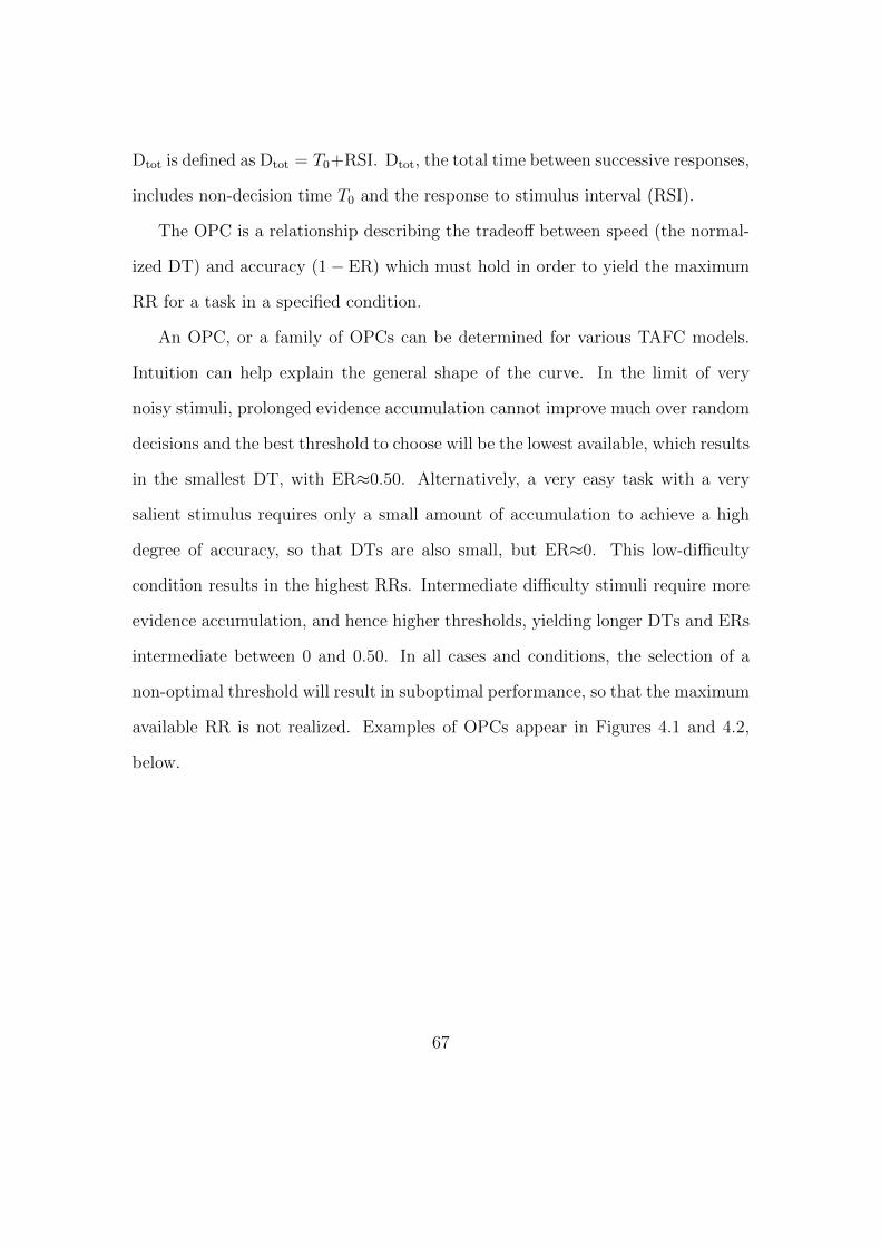
Dtot is defined as Dtot = T0+RSI. Dtot, the total time between successive responses,

includes non-decision time T0 and the response to stimulus interval (RSI).

The OPC is a relationship describing the tradeoff between speed (the normal-

ized DT) and accuracy (1− ER) which must hold in order to yield the maximum

RR for a task in a specified condition.

An OPC, or a family of OPCs can be determined for various TAFC models.

Intuition can help explain the general shape of the curve. In the limit of very

noisy stimuli, prolonged evidence accumulation cannot improve much over random

decisions and the best threshold to choose will be the lowest available, which results

in the smallest DT, with ER≈0.50. Alternatively, a very easy task with a very

salient stimulus requires only a small amount of accumulation to achieve a high

degree of accuracy, so that DTs are also small, but ER≈0. This low-difficulty

condition results in the highest RRs. Intermediate difficulty stimuli require more

evidence accumulation, and hence higher thresholds, yielding longer DTs and ERs

intermediate between 0 and 0.50. In all cases and conditions, the selection of a

non-optimal threshold will result in suboptimal performance, so that the maximum

available RR is not realized. Examples of OPCs appear in Figures 4.1 and 4.2,

below.

67

Optimal Performance under the Pure DDM is Described by a Unique

Curve

The pure DDM is unique in that it has a parameter-free OPC, defined by the

function:

DT

Dtot

=

(1

ER log 1−ERER

+1

1− 2ER

)−1

, (4.15)

as derived in [10]. This function, which relates two key behavioral quantities is

illustrated in solid black in Figures 4.1 and 4.2(a,b). See [10, 134] for derivations

and further discussion of the OPC.

Optimal Performance under the Extended DDM is Not Uniquely De-

fined

The extended DDM has families of OPCs rather than a unique OPC, as in the

pure DDM. In the extended DDM, variability in initial conditions precludes the

possibility of trials with a DT = 0. However, for low values of the variance

parameters in the extended DDM, the OPCs for the extended DDM approach the

OPC for the pure DDM. A sample OPC for the extended DDM is illustrated in

the dashed line in Figure 4.1. To compute these curves, we fixed all parameters

except drift rate and threshold. For each drift rate, we found the threshold which

optimized RR and used this threshold to determine ER and normalized DT. For

more details, the reader is referred to [10].

68

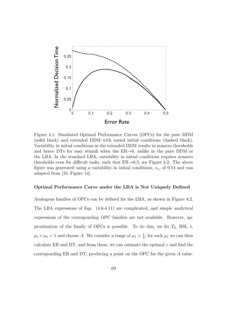
Threshold-Setting Algorithms

Above, in the section Optimal Thresholds for Different Criteriain the Pure DDM, we derived expressions for the thresholds thatoptimize various criteria for a given set of task parameters. Thisraises the question, How do decision makers identify this optimalthreshold? In this section, we review published work addressingthis question, and we show that any adaptive threshold-settingmodel makes two predictions for a task in which participantsmaximize RR: (a) They will choose thresholds closer to optimalvalues for easier versus harder tasks, and (b) they will tend tochoose thresholds at higher than optimal values.

One possibility is that the knowledge of optimal threshold isintrinsic; that is, the decision maker comes to the task with com-plete knowledge of the relationship between task parameters (sig-nal, noise, delay, and their variability) and the optimal threshold.Although this may be possible for highly practiced tasks within anarrow domain of parameters, it seems unlikely more generallyand certainly for novel tasks. Here, we consider the more plausible(or at least more general) alternative that the decision maker has nointrinsic knowledge of the optimal threshold but is able to deter-

mine (or approximate) it using an adaptive adjustment procedure:Different values of the threshold are sampled, the effects on acriterion are observed, and the threshold is adjusted to optimize thecriterion.18 Several studies have examined this possibility.

Review of Threshold Setting

Myung and Busemeyer (1989) performed an experiment usingthe free-response paradigm19 in which participants were explicitlyrequired to minimize BR. They tested predictions of two algo-

18 Note that such an adaptive mechanism is likely to be required even ifthe relationship of task parameters to optimal threshold is known. This isbecause unless the task parameters are explicitly specified at the outset,they must be discovered. This, in turn, requires sampling at some thresholdthat is most likely not optimal (because the optimal one is not yet known)and that therefore must be adapted as the task parameters are discovered.

19 In this experiment, participants were presented with successive “re-sults of medical tests” until they made a choice of “diagnosis.” Thus, DT(in the equation for BR) for this experiment corresponded to the number ofmedical tests the participant observed before the diagnosis.

a) b)

0 0.5 10.1

0.15

0.2

0.25

Drift variability

Opt

imal

thr

esho

ld

0 0.1 0.20.1

0.15

0.2

0.25

Starting point variability

Opt

imal

thr

esho

ld

c) d)

0 0.1 0.2 0.3 0.4 0.50

0.05

0.1

0.15

0.2

0.25

Error rate

Mea

n no

rmal

ized

dec

isio

n tim

e sA=0, sx=0

sA=0, sx=0.14

sA=0.31, sx=0

0 0.1 0.2 0.3 0.4 0.50

0.05

0.1

0.15

0.2

0.25

Error rate

Mea

n no

rmal

ized

dec

isio

n tim

e sA=0, sx=0

sA=0, sx=0.14

sA=0.31, sx=0

!

0

Figure 14. Optimal thresholds and optimal performance curves for the extended drift diffusion model (DDM).a, b: Dependence of the reward-rate-maximizing threshold for the extended DDM on drift variability (Panel a)and starting point variability (Panel b), with other parameters held fixed. The values of the varied parameters areshown on horizontal axes, and the values of the fixed parameters were equal to sx ! 0.14, mA ! 1, sA ! 0.31,c ! 0.33 (corresponding to values estimated from a sample participant; see Figure 5), and Dtotal ! 2 (one of thedelay conditions performed by the participant). c, d: Optimal performance curves for the extended DDM,obtained numerically by varying noise parameter c while other parameters were kept fixed: mA ! 1, sx and sA

as shown in figure legend, Dtotal ! 2 in Panel c, and Dtotal ! 0.5 in Panel d.

727OPTIMAL DECISION MAKING

Figure 4.1: Simulated Optimal Performance Curves (OPCs) for the pure DDM(solid black) and extended DDM with varied initial conditions (dashed black).Variability in initial conditions in the extended DDM results in nonzero thresholdsand hence DTs for easy stimuli when the ER→0, unlike in the pure DDM orthe LBA. In the standard LBA, variability in initial conditions requiresnonzero thresholds even for tasks with high signal, such that ER→0,as we see in the following figure. The above figure was adapted fromFigure 14 on page 727 of [10].

Optimal Performance Curve under the LBA is Not Uniquely Defined

Analogous families of OPCs can be defined for the LBA, as shown in Figure 4.2.

The LBA expressions of Equations 4.6-4.11 are complicated, and simple analyt-

ical expressions of the corresponding OPC families are not available. However,

approximation of the family of OPCs is possible. To do this, we fix T0, RSI, s,

µ1 +µ2 = 1 and choose A. We consider a range of µ1 > 12; for each µ1 we can then

calculate ER and DT, and from them, we can estimate the optimal z and find the

corresponding ER and DT, producing a point on the OPC for the given A value.

69

Error Rate

Nor

mal

ized

Dec

isio

n T

ime

Figure 4.1: Simulated Optimal Performance Curves (OPCs) for the pure DDM(solid black) and extended DDM with varied initial conditions (dashed black).Variability in initial conditions in the extended DDM results in nonzero thresholdsand hence DTs for easy stimuli when the ER→0, unlike in the pure DDM orthe LBA. In the standard LBA, variability in initial conditions requires nonzerothresholds even for difficult tasks, such that ER→0.5, see Figure 4.2. The abovefigure was generated using a variability in initial conditions, sx, of 0.14 and wasadapted from [10, Figure 14].

Optimal Performance Curve under the LBA is Not Uniquely Defined

Analogous families of OPCs can be defined for the LBA, as shown in Figure 4.2.

The LBA expressions of Eqs. (4.6-4.11) are complicated, and simple analytical

expressions of the corresponding OPC families are not available. However, ap-

proximation of the family of OPCs is possible. To do this, we fix T0, RSI, s,

µ1 +µ2 = 1 and choose A. We consider a range of µ1 >12; for each µ1 we can then

calculate ER and DT, and from them, we can estimate the optimal z and find the

corresponding ER and DT, producing a point on the OPC for the given A value.

69

We find that a different OPC is generated for each value of A, showing that there

is no unique OPC for the LBA model.

This observation is consistent with the observation that, for any µ1 = µ2 = µ

(equal evidence for both options), the expected accuracy will be exactly 0.50 and

no additional accuracy may be realized or information accumulated over time. It

follows that the optimal threshold is then the lowest possible threshold. For the

pure DDM and the extended DDM with zero initial condition variance (sx = 0),

the threshold parameter, z, can go to 0, while in the LBA, the threshold must

lie at or above the top of the range of initial conditions, i.e., z ≥ A. The lowest

threshold, and the optimal threshold for µ1 = µ2 = µ is then z = A. The OPC

curve plotting DTDTtot

therefore varies with the value of A as shown in Figure 4.2(a):

the smooth portions of each curve correspond to z > A (on the left) and z = A

(on the right). We see that there are multiple OPCs for the LBA, one for each

value of A; moreover, unlike the OPC for the DDM, these curves terminate at ER

= 0.5 with finite normalized DTs.

We therefore also consider an adapted version of the LBA, such that the thresh-

olds are allowed to fall within the range of initial conditions as well as above it, and

show that the OPC for this adapted LBA is also not unique. If one of the initial

conditions in a trial falls above the threshold value, the DT for that particular

trial is then 0. If both of the initial conditions in a trial are above the threshold,

then the option corresponding to the larger initial condition is selected, and the

decision time is again 0. The mean DT and ER, ERa and DTa, for this adapted

70

0 0.05 0.1 0.15 0.2 0.25 0.3 0.35 0.4 0.45 0.50

0.05

0.1

0.15

0.2

0.25

Error Rate

Nor

mal

ized

Dec

isio

n T

ime

Standard LBA CurvesThreshold z ≥ A

A = 500A = 400A = 300A = 200A = 100

(a)

0 0.05 0.1 0.15 0.2 0.25 0.3 0.35 0.4 0.45 0.50

0.05

0.1

0.15

0.2

0.25

Error Rate

Nor

mal

ized

Dec

isio

n T

ime

Adapted LBA CurvesThreshold z ≥ 0

A = 500A = 400A = 300A = 200A = 100

(b)

Figure 4.2: Simulated Optimal Performance Curves (OPCs) for the LBA. We seethat OPCs for both the standard LBA (a) and adapted LBA, in which thresholdz is allowed to go to 0 (b) are not unique. The following parameters were usedin the simulation: s = 0.32, T0 = 226 ms, RSI=1000ms, µ1 + µ2 = 1. The OPCpredicted by the pure DDM is shown in black.

system with z < A are defined accordingly:

ERa(A, z, µ1, µ2, s) =1

2· A− z

A+z

A· ER(z, z, µ1, µ2, s), (4.16)

DTa(A, z, µ1, µ2, s) =z

A·DT(z, z, µ1, µ2, s), (4.17)

in which ER and DT are calculated as above for the standard LBA model.

Numerically derived OPCs for this adapted LBA are shown in Figure 4.2(b).

In the case of µ1 = µ2 = 12, it allows the optimal threshold z∗ = 0, and so limits in

the desired point at which DT is 0 and the ER is 0.50. This is because a higher

value of z would not result in any change in accuracy, so the best value of z is the

one which minimizes DT. Moreover, as µ1 → µ2, we expect z∗ → 0. Similarly, for

µ1 >> µ2, we expect low ER and corresponding low DT, due to high bias towards

correct choices.

71

The smooth portion of the curve to the left starting at ER=0 corresponds to

z > A, and that to the right ending at ER=0.5 corresponds to z < A. The kink

between these segments represents a jump between endpoints of these two ranges

for z. For this parameterization and simulation, z = A is never optimal. The

adapted LBA predicts that optimal behavior will not result in ERs lying between

these two ranges.

In the degenerate case A = 0, no additional accuracy is gained by having a

nonzero z as there is no noise in initial conditions, so that z∗ is always 0, not just

at the case µ1 = µ2 = µ. Thus, as A → 0, we expect that z∗ → 0, even when

µ1 6= µ2: OPC curves get flatter for every ER, such that the normalized DTs get

smaller and smaller, as seen in the plot.

Noise Scales Differently in the pure DDM and LBA

We compare noise scaling in the two models and note that as noise increases, the

models behave differently. Noise levels can be high in certain TAFC settings, such

as those considered later in this chapter. The signal to noise ratio is varied from

one condition to the next, but this variation can be accounted for in the models

by allowing mean drift rates to change, so that comparisons of the role of noise

alone in the DDM and LBA should be meaningful. We consider additive noise in

the pure DDM, and in the LBA we also consider variability in both the drift rate s

and range of initial conditions A. As the noise parameters are intended to remain

analogous between models, differences between noise in the models is noteworthy.

72

Scaling in the Pure DDM for High Noise

We consider approximations of ER( 1σ2 ) and DT( 1

σ2 ) about the point ER( 1σ2 = 0)

and DT( 1σ2 = 0) We can Taylor expand the DDM expressions with respect to small

parameter 1σ2 :

ER =1

2− zµ

2

(1

σ2

)+z3µ3

6

(1

σ6

)+O

(z5µ5

σ10

)(4.18)

DT = z2

(1

σ2

)− µ2z4

3

(1

σ6

)+O

(µ4z6

σ10

)(4.19)

We see that ER is O (1), and DT is O(

1σ2

)with respect to 1

σ2 : ER scales

differently with high noise σ than does DT. However, both ER and DT are of

the same order with respect to σ2. In particular, taking limits as σ → ∞, we

find that ER→ 0.5 and DT→ 0. Intuitively, we see that large noise pushes the

accumulation process very rapidly away from the initial condition and towards one

of the boundaries. For difficult tasks, we then expect ER=0.5 and DT=0 to lie on

the OPC for the pure DDM, as it does.

We now consider the scaling of ER and DT with noise parameters in the LBA.

We will see that large noise in the LBA generally leads to nonzero DTs.

Scaling in the Standard LBA in the case µ1 = µ2

The LBA has two sources of noise or variability in the case of non-discriminable

stimuli (µ1 = µ2 = 12). The first source of noise is the variability in drift rates, s,

and the second is the variability in initial conditions, A.

In both cases, as the two drift rates µ1 and µ2 are equivalent, and as drift is the

only source of bias in the LBA model, the ER is 0.5. We note that the mean DT

73

can be 0 if and only if A = 0. This restriction on the DT follows from the constraint

that z ≥ A, so that a nonzero A implies a nonzero mean distance to accumulate

to threshold. To see this, first suppose that s = 0 and then allow s to increase,

producing a distribution of drift rates centered around µi = 12. Moreover, as A

increases, the minimum allowable value of the threshold z also increases because

zmin = A. It follows that for µ1 = µ2 and the minimum z, DT increases with the

value of A.

These behaviors for µ1 = µ2 and high A or s are quite different from those seen

in the pure DDM, in which large noise implies DT→ 0.

4.2.3 Reward Maximization Experiment

We consider here human performance in a motion discrimination task previously

presented and analyzed in [6]. Participants (n = 17, 6 male) were tasked to dis-

criminate the direction of moving dots on a computer screen. The participants

viewed the stimuli at approximately 2 feet from the CRT monitor on which they

were presented and indicated the direction of motion via keypress on a standard

keyboard. Participants could indicate leftward motion with the ‘Z’ key and right-

ward motion with the ‘M’ key. The experiments were conducted at a Macintosh

computer, using the Psychophysics Toolbox [14]. Each participant completed at

least 13 daily sessions of 60 minutes duration.

The first four sessions involved training and practice activities in which par-

ticipants did not receive monetary reward. In later sessions, participants first

completed five blocks of a motion discrimination task, with each block presented

at a different coherence (0, 4, 8, 16, and 32%, randomized across participants); par-

74

ticipants earned $0.02 for each correct response. Performance improved markedly

over the first 5 sessions and for certain participants continued to improve until

session 9. Here we only use data from sessions 10-13. Premature responses, either

anticipatory or with RTs of less than 100 ms, were penalized with a buzzing sound

and a 4 second timeout period. When participants did not respond prematurely,

a response to stimulus interval was selected from an exponential distribution with

mean of 1 second.

After they completed the free response motion discrimination task, partici-

pants performed an interval timing task and then a signal detection task. The

setup of the signal detection task was the same as that of the Rmax task, except

participants were instructed to indicate the onset of dot motion, regardless of its

direction. In one block they would be instructed to press the ‘M’ key, and in the

other, the ‘Z’ key. They again received $0.02 for each correct (non-anticipatory)

response. For more details, the reader is referred to [6].

In this chapter, we consider only the results of the reward maximization and

signal detection tasks.

4.2.4 Data Fitting Procedures

Fits were performed to participant data from the task above for the two DDMs

and the LBA using published toolboxes for the models in Matlab [125] and R [38],

respectively. Fitting the data to the LBA model required some modifications to

the standard LBA code, as outlined in [38]. Data were separated for individual

participants by difficulty condition. Fits were computed for each individual par-

ticipant over all five difficulty conditions. Multiple fits were performed for each

75

condition and participant, first varying only caution (threshold) with difficulty

level, and then varying the range of initial conditions as well, while the remaining

parameters were held constant. The same data and partitioning of data, was used

for both model fit toolboxes.

The DDM and LBA models in this chapter were fit separately to distributions

of RTs for correct and error trials in each condition because the two fit toolboxes

have been designed to fit properties of distributions of RTs rather than mean

values. A primary goal of the work in this chapter is to compare the efficacy of

the models, and the least biased way to do this is via the corresponding toolboxes

designed to fit the models. Both toolboxes allow the user to set constraints such

that certain parameters are held constant while others are allowed to vary from

one condition to the next. The DDM toolbox does this by using a combination of

a system of matrix equations similar to those in general linear models coupled with

post-processing to remove outliers [127, 128]. The LBA toolbox uses the quantile

maximum probability estimator method [55] to estimate the parameters of density

functions for distributions for correct and error trials, and these parameters can

then be used to select model parameters. In all cases, fits were performed on the

10-90th quantiles for correct and error trials. In contrast, the models in Chapters

2 and 3 were fit only to mean RT and ER for correct and error trials data using

the least squares method.

The goodness of fit for each model prediction of mean RT and ER for each

condition and participant was then assessed using Akaike, Corrected Akaike, and

Bayesian Information Criteria, as described in the first chapter of this thesis. Fi-

nally, in addition to modeling the way participants actually performed on the task,

their theoretical optimal performance for each difficulty condition or drift rate

76

could be estimated by allowing the caution parameter to vary freely while holding

all the other parameters constant. The optimal value of the caution parameter is

defined as that which results in the highest possible reward rate (a combination of

rapid RT and/or low ER), given fixed (fitted) values for the remaining parameters.

4.3 Results

In order to determine relative suitability of DDM and LBA models for reward

maximization task data, we analyze fits in several ways. We fit each individual

participant in the following models:

• A pure DDM, in which only the thresholds z vary between the coherence

conditions.

• An extended DDM, in which only the thresholds z vary between coherence

conditions.

• A second extended DDM, in which both the thresholds z and range of initial

conditions sx vary between coherence conditions.

• A LBA model, in which only the thresholds z vary between the coherence

conditions.

• A second LBA model, in which both the thresholds z and the range of initial

conditions A vary between coherence conditions.

Fits to mean RT and ER data for each participant and condition were quite

good for each model: the mean value of the correlation coefficient, R2, was greater

than or equal to 0.95 for each of the models. Mean AIC, AICc, and BIC values for

77

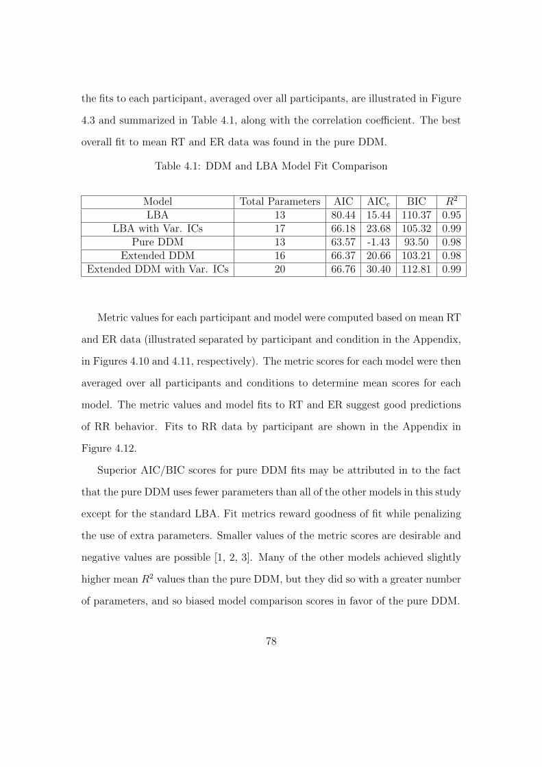
the fits to each participant, averaged over all participants, are illustrated in Figure

4.3 and summarized in Table 4.1, along with the correlation coefficient. The best

overall fit to mean RT and ER data was found in the pure DDM.

Table 4.1: DDM and LBA Model Fit Comparison

Model Total Parameters AIC AICc BIC R2

LBA 13 80.44 15.44 110.37 0.95LBA with Var. ICs 17 66.18 23.68 105.32 0.99

Pure DDM 13 63.57 -1.43 93.50 0.98Extended DDM 16 66.37 20.66 103.21 0.98

Extended DDM with Var. ICs 20 66.76 30.40 112.81 0.99

Metric values for each participant and model were computed based on mean RT

and ER data (illustrated separated by participant and condition in the Appendix,

in Figures 4.10 and 4.11, respectively). The metric scores for each model were then

averaged over all participants and conditions to determine mean scores for each

model. The metric values and model fits to RT and ER suggest good predictions

of RR behavior. Fits to RR data by participant are shown in the Appendix in

Figure 4.12.

Superior AIC/BIC scores for pure DDM fits may be attributed in to the fact

that the pure DDM uses fewer parameters than all of the other models in this study

except for the standard LBA. Fit metrics reward goodness of fit while penalizing

the use of extra parameters. Smaller values of the metric scores are desirable and

negative values are possible [1, 2, 3]. Many of the other models achieved slightly

higher mean R2 values than the pure DDM, but they did so with a greater number

of parameters, and so biased model comparison scores in favor of the pure DDM.

78

We note some differences between the fit scores: allowing the range of initial

conditions to vary in the LBA results in a superior fit with regard to each of the

metrics except AICc. However, for the extended DDM, allowing the range of initial

conditions to vary does not improve model fits according to any of the metrics.

We note that we are fitting a small data set of mean RT and ER measure-

ments for each subject spread over five difficulty conditions. We consider RT

and ER because they are traditionally of greatest interest in modeling Rmax task

behavior. When comparing the pure DDM fit to the two extended DDM fits

over the entire distribution of RTs instead using the DDM toolbox, the extended

DDM (χ2 = 168.35, p < 0.05) and extended DDM with variable initial conditions

(χ2 = 408.94, p < 0.001) yield superior deviance scores [27]. However, fitting the

entire distribution is not a goal of this work, so for our purposes the pure DDM

provides the superior diffusion model fit.

Fits for each of the models and participants provided good qualitative matches

to the ER and corresponding estimated normalized DT data, for which non-

decision times T0 were estimated for each participant from the mean RTs for the

fastest 25% of their signal detection trials, as in [6, 5].

The high performing participants generally had ERs and normalized DTs close

to those on the OPC for the pure DDM. Figure 4.4 shows fits to the behavior for one

representative higher performing and one lower performing participant (Subjects

32 and 34). Figure 4.5 shows the means averaged over all subjects. In each figure,

the data is shown in solid black with error bars, and fits are superimposed in

curves of various colors. As with individual subjects, the average behavior trends

away from the OPC for the pure DDM as ERs increase. The LBA models and

the pure DDM overestimate normalized DTs and the extended DDMs slightly

79

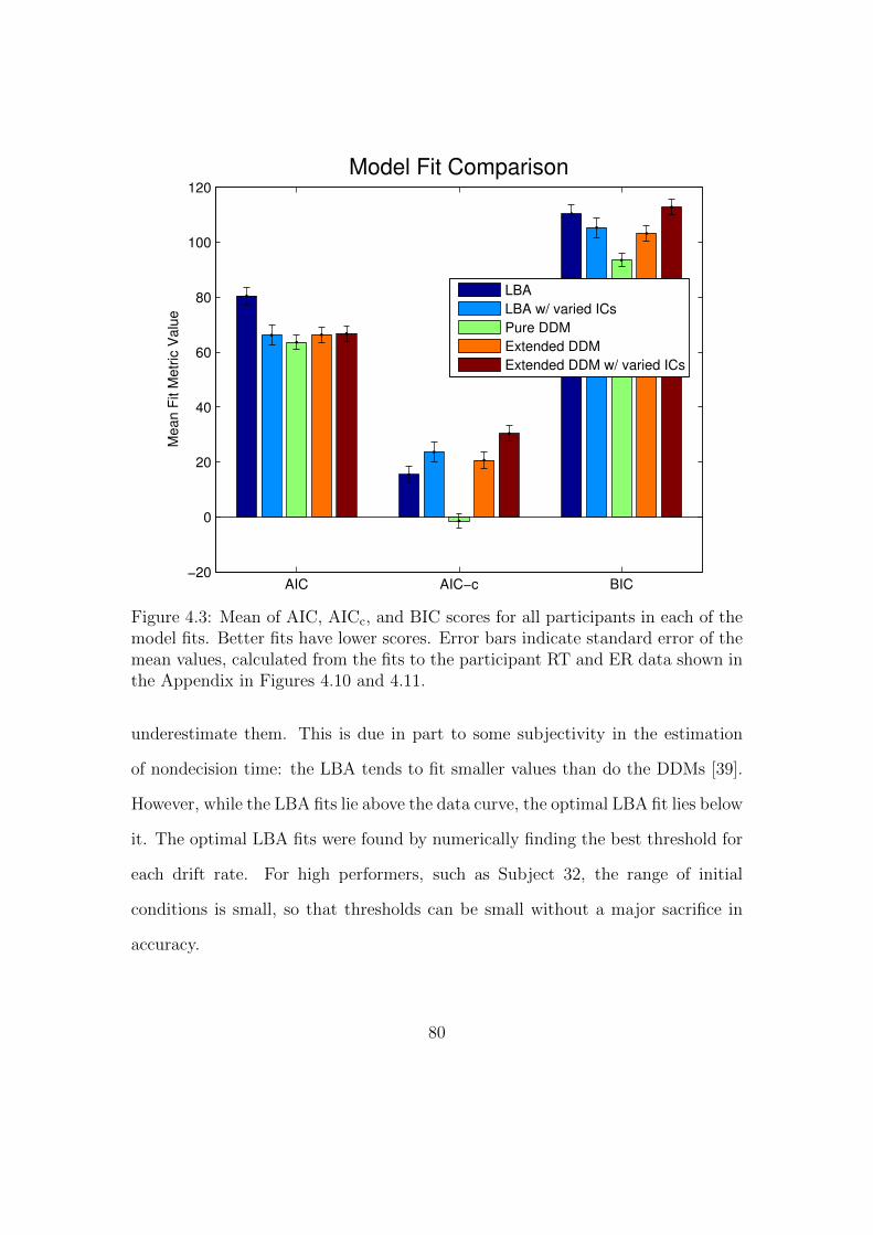
AIC AIC−c BIC−20

0

20

40

60

80

100

120M

ea

n F

it M

etr

ic V

alu

eModel Fit Comparison

LBA

LBA w/ varied ICs

Pure DDM

Extended DDM

Extended DDM w/ varied ICs

Figure 4.3: Mean of AIC, AICc, and BIC scores for all participants in each of themodel fits. Better fits have lower scores. Error bars indicate standard error of themean values, calculated from the fits to the participant RT and ER data shown inthe Appendix in Figures 4.10 and 4.11.

underestimate them. This is due in part to some subjectivity in the estimation

of nondecision time: the LBA tends to fit smaller values than do the DDMs [39].

However, while the LBA fits lie above the data curve, the optimal LBA fit lies below

it. The optimal LBA fits were found by numerically finding the best threshold for

each drift rate. For high performers, such as Subject 32, the range of initial

conditions is small, so that thresholds can be small without a major sacrifice in

accuracy.

80

The difference between this empirical normalized DT and the corresponding

normalized model DT (the OPC for the pure DDM) was a good predictor of over-

all RR for each of the difficulty conditions (R2 = 0.53, p < 0.001). Fits for all

participants can be found in the Appendix in Figure 4.13. In each of the panels

of the figure, we also included an LBA OPC, which represents optimal behavior

given the participant’s estimated parameters for drift, variability in drift, range

of initial conditions, and nondecision time, from which the optimal threshold can

be numerically determined. We note that for many high performing participants,

including Subject 32, the predicted LBA OPC lies below the model fits to behav-

iors for intermediate ERs. We will see later that this is to be expected due to

restrictions placed on the range of initial conditions A to match both long and

short RTs in different difficulty conditions.

In order to better understand differences between the model fits, we considered

the mean parameter fits for the caution parameter. That is, for each participant,

difficulty condition, and DDM fit, we calculated a threshold, and then we averaged

over all the individual threshold values for a given model and difficulty condition.

The resulting mean threshold values are shown in Figure 4.6. We see that on aver-

age, for the pure DDM and extended DDM with fixed range of initial conditions for

all coherences, the threshold values increase with coherence. Allowing the range

of initial conditions in the DDM to vary with coherence also produces thresholds

that vary significantly with coherence (F (4, 64) = 73.72, p < 0.01, η2 = 0.82).

We next compare mean values of the threshold parameter, averaged across

participants, in the two LBA model fits in Figure 4.7. In the first LBA fit, only

the threshold is allowed to vary by condition, and the trend in participant caution

is consistent with that shown by the first two DDMs: thresholds modestly increase

81

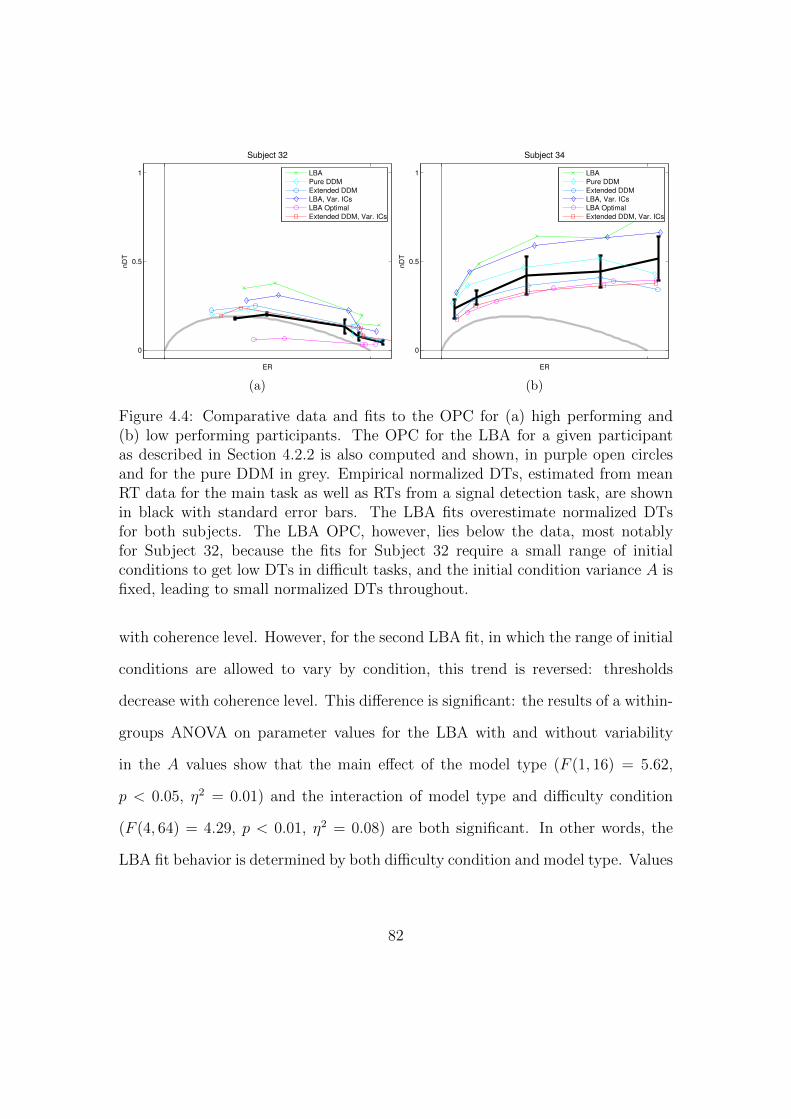
0

0.5

1

ER

nD

T

Subject 32

LBA

Pure DDM

Extended DDM

LBA, Var. ICs

LBA Optimal

Extended DDM, Var. ICs

(a)

0

0.5

1

ER

nD

T

Subject 34

LBA

Pure DDM

Extended DDM

LBA, Var. ICs

LBA Optimal

Extended DDM, Var. ICs

(b)

Figure 4.4: Comparative data and fits to the OPC for (a) high performing and(b) low performing participants. The OPC for the LBA for a given participantas described in Section 4.2.2 is also computed and shown, in purple open circlesand for the pure DDM in grey. Empirical normalized DTs, estimated from meanRT data for the main task as well as RTs from a signal detection task, are shownin black with standard error bars. The LBA fits overestimate normalized DTsfor both subjects. The LBA OPC, however, lies below the data, most notablyfor Subject 32, because the fits for Subject 32 require a small range of initialconditions to get low DTs in difficult tasks, and the initial condition variance A isfixed, leading to small normalized DTs throughout.

with coherence level. However, for the second LBA fit, in which the range of initial

conditions are allowed to vary by condition, this trend is reversed: thresholds

decrease with coherence level. This difference is significant: the results of a within-

groups ANOVA on parameter values for the LBA with and without variability

in the A values show that the main effect of the model type (F (1, 16) = 5.62,

p < 0.05, η2 = 0.01) and the interaction of model type and difficulty condition

(F (4, 64) = 4.29, p < 0.01, η2 = 0.08) are both significant. In other words, the

LBA fit behavior is determined by both difficulty condition and model type. Values

82

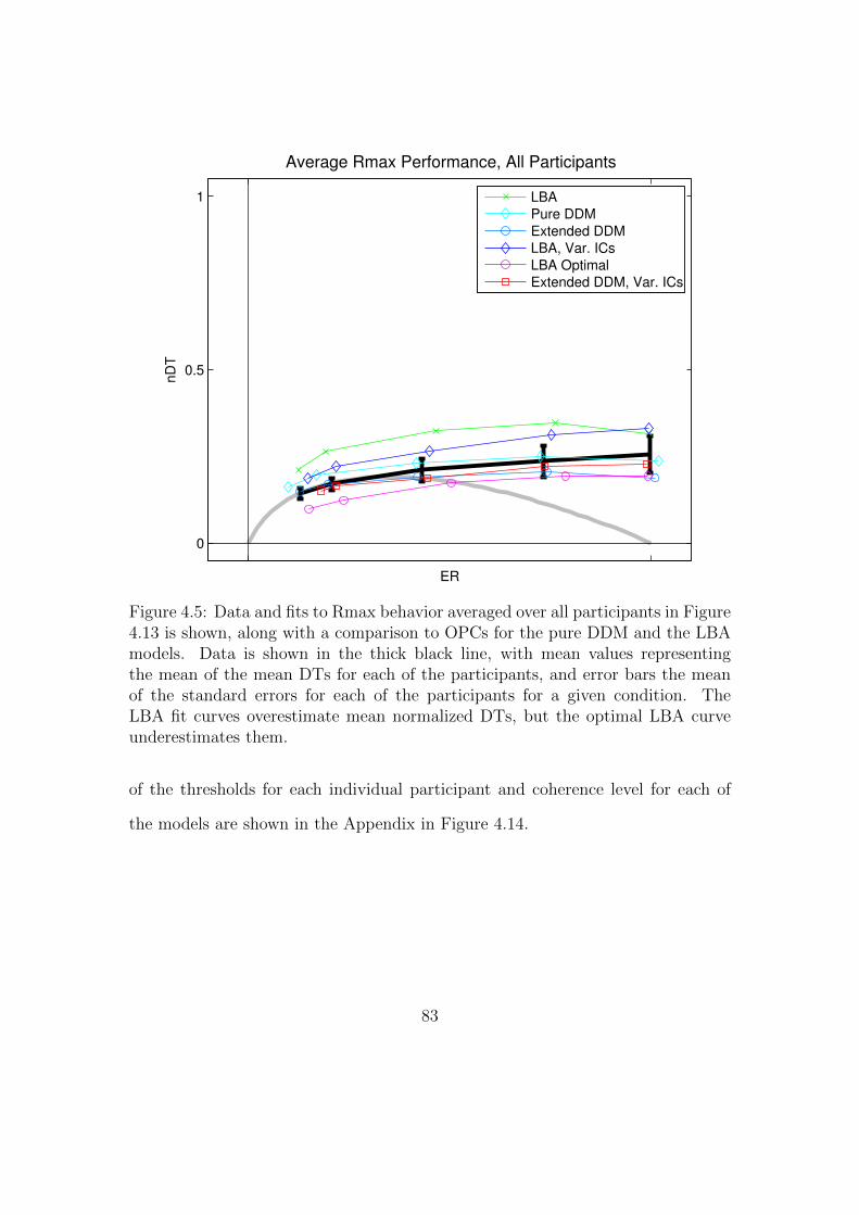
0

0.5

1

ER

nD

TAverage Rmax Performance, All Participants

LBA

Pure DDM

Extended DDM

LBA, Var. ICs

LBA Optimal

Extended DDM, Var. ICs

Figure 4.5: Data and fits to Rmax behavior averaged over all participants in Figure4.13 is shown, along with a comparison to OPCs for the pure DDM and the LBAmodels. Data is shown in the thick black line, with mean values representingthe mean of the mean DTs for each of the participants, and error bars the meanof the standard errors for each of the participants for a given condition. TheLBA fit curves overestimate mean normalized DTs, but the optimal LBA curveunderestimates them.

of the thresholds for each individual participant and coherence level for each of

the models are shown in the Appendix in Figure 4.14.

83

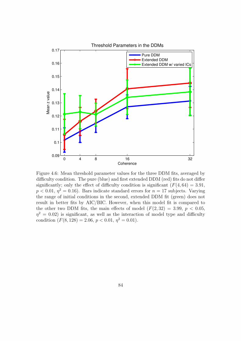
0 4 8 16 320.09

0.1

0.11

0.12

0.13

0.14

0.15

0.16

0.17

Threshold Parameters in the DDMs

Coherence

Mean z

valu

e

Pure DDM

Extended DDM

Extended DDM w/ varied ICs

Figure 4.6: Mean threshold parameter values for the three DDM fits, averaged bydifficulty condition. The pure (blue) and first extended DDM (red) fits do not differsignificantly; only the effect of difficulty condition is significant (F (4, 64) = 3.91,p < 0.01, η2 = 0.16). Bars indicate standard errors for n = 17 subjects. Varyingthe range of initial conditions in the second, extended DDM fit (green) does notresult in better fits by AIC/BIC. However, when this model fit is compared tothe other two DDM fits, the main effects of model (F (2, 32) = 3.99, p < 0.05,η2 = 0.02) is significant, as well as the interaction of model type and difficultycondition (F (8, 128) = 2.06, p < 0.01, η2 = 0.01).

84

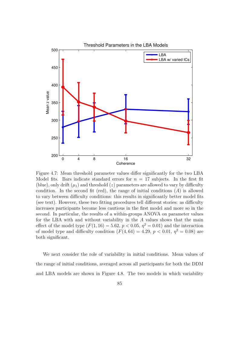
0 4 8 16 32200

250

300

350

400

450

500

Threshold Parameters in the LBA Models

Coherence

Me

an

z v

alu

e

LBA

LBA w/ varied ICs

Figure 4.7: Mean threshold parameter values differ significantly for the two LBAModel fits. Bars indicate standard errors for n = 17 subjects. In the first fit(blue), only drift (µ1) and threshold (z) parameters are allowed to vary by difficultycondition. In the second fit (red), the range of initial conditions (A) is allowedto vary between difficulty conditions: this results in significantly better model fits(see text). However, these two fitting procedures tell different stories: as difficultyincreases participants become less cautious in the first model and more so in thesecond. In particular, the results of a within-groups ANOVA on parameter valuesfor the LBA with and without variability in the A values shows that the maineffect of the model type (F (1, 16) = 5.62, p < 0.05, η2 = 0.01) and the interactionof model type and difficulty condition (F (4, 64) = 4.29, p < 0.01, η2 = 0.08) areboth significant.

We next consider the role of variability in initial conditions. Mean values of

the range of initial conditions, averaged across all participants for both the DDM

and LBA models are shown in Figure 4.8. The two models in which variability

85

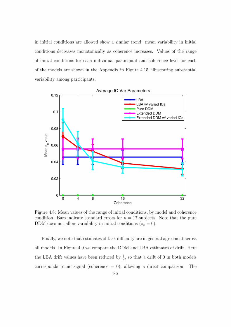
in initial conditions are allowed show a similar trend: mean variability in initial

conditions decreases monotonically as coherence increases. Values of the range

of initial conditions for each individual participant and coherence level for each

of the models are shown in the Appendix in Figure 4.15, illustrating substantial

variability among participants.

0 4 8 16 320

0.02

0.04

0.06

0.08

0.1

0.12

Average IC Var Parameters

Coherence

Me

an

sx v

alu

e

LBA

LBA w/ varied ICs

Pure DDM

Extended DDM

Extended DDM w/ varied ICs

Figure 4.8: Mean values of the range of initial conditions, by model and coherencecondition. Bars indicate standard errors for n = 17 subjects. Note that the pureDDM does not allow variability in initial conditions (sx = 0).

Finally, we note that estimates of task difficulty are in general agreement across

all models. In Figure 4.9 we compare the DDM and LBA estimates of drift. Here

the LBA drift values have been reduced by 12, so that a drift of 0 in both models

corresponds to no signal (coherence = 0), allowing a direct comparison. The

86

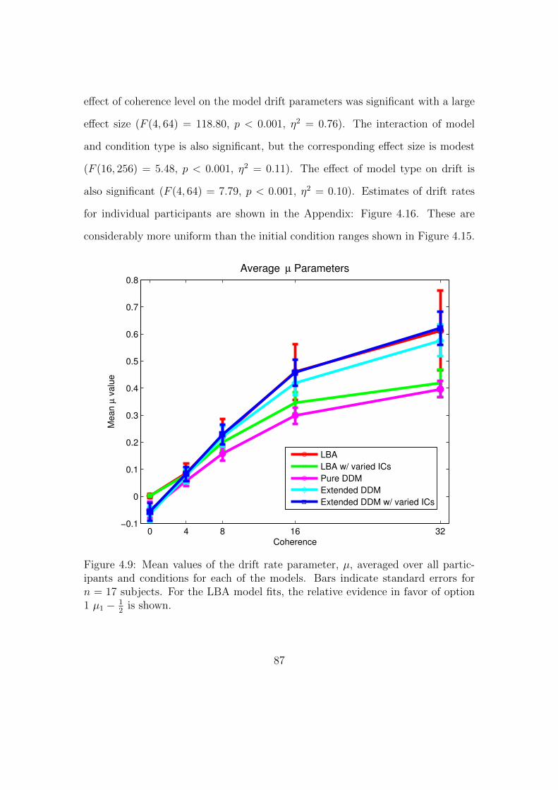
effect of coherence level on the model drift parameters was significant with a large

effect size (F (4, 64) = 118.80, p < 0.001, η2 = 0.76). The interaction of model

and condition type is also significant, but the corresponding effect size is modest

(F (16, 256) = 5.48, p < 0.001, η2 = 0.11). The effect of model type on drift is

also significant (F (4, 64) = 7.79, p < 0.001, η2 = 0.10). Estimates of drift rates

for individual participants are shown in the Appendix: Figure 4.16. These are

considerably more uniform than the initial condition ranges shown in Figure 4.15.

0 4 8 16 32−0.1

0

0.1

0.2

0.3

0.4

0.5

0.6

0.7

0.8

Average µ Parameters

Coherence

Mean µ

valu

e

LBA

LBA w/ varied ICs

Pure DDM

Extended DDM

Extended DDM w/ varied ICs

Figure 4.9: Mean values of the drift rate parameter, µ, averaged over all partic-ipants and conditions for each of the models. Bars indicate standard errors forn = 17 subjects. For the LBA model fits, the relative evidence in favor of option1 µ1 − 1

2is shown.

87

4.4 Discussion

We compared the DDM and LBA accounts of behavior in an Rmax task. In the

context of the DDM, the adjustment of a caution or threshold parameter is known

to be integral to describing Rmax behavior [10, 6]. For example, participants

either adjust the threshold to best suit each difficulty condition, or they may pick

a single threshold level which works well, but not optimally, across blocks of various

difficulty levels [6].

We first compared the DDM and LBA accounts of behavior in the context of

optimal performance theory. We showed that, while the OPC for the pure DDM

is a single, unique curve, the OPCs for the LBA, like those for the extended DDM

are non-unique. We also showed that, for a given set of parameters, the best

behavior possible in the LBA is at least partially determined by the value of the

range of initial conditions. With a nonzero range of initial conditions, uniformly

quick responses at near signal detection speed are impossible. Further, when the

range of initial conditions in the LBA, A, is set at or near 0, the quality of fits is

limited. Nonetheless, allowing A to vary from coherence to coherence allows for

significantly better data fits and this parameter variability is consequently critical

to the success of the model.

Implications for the identification of an OPC for LBA parameters are illustrated

in Figure 4.2: we found that the shape of the OPC depended upon the allowed

range of initial conditions. Smaller, more restricted ranges of initial conditions

result in flatter OPCs.

We then applied various DDM and LBA accounts of behavior to an Rmax

data set. We considered several models: a pure DDM, an extended DDM, and a

88

standard LBA fit in which drift and threshold varied by difficulty condition. We

also considered fits to the extended DDM and to the LBA in which the range

of initial conditions was allowed to vary from one coherence level to the next.

We showed in Table 4.1 and Figure 4.3 that LBA matches to behavior were best

when both the range of initial conditions and the thresholds were allowed to vary

with coherence. For similarly good matches to behavior, such manipulation of

initial conditions was unnecessary in the DDMs we considered. For consistency, we

employed the standard LBA parameterization as described in [20, 39] to generally

follow that of the extended DDM.

That initial condition variability is critical in the LBA is to be expected, as we

found that the ability to achieve short RTs (and corresponding estimated DTs)

in the LBA model is directly influenced by the range of initial conditions, A, as

shown in Figure 4.2(a).

Our measurements of average fit quality were consistent with the expected

importance of variability in initial conditions when accounting for Rmax behavior

in the LBA: quality of fit metrics AIC, AICc, and BIC were better for the LBA

model in which variance in initial conditions was allowed than for the fits in which

this variation was held constant. Averaged over all participants, values of the

three fit metrics for each model are illustrated in Figure 4.3. In the second LBA fit,

participants mostly reduced caution and also reduced the range of initial conditions

in higher coherence blocks: see Figures 4.7 and 4.8. Significantly, in the first

LBA fit, with constant variance in initial conditions, participants instead modestly

increased caution with coherence, as they did in all three DDM fits (compare

Figures 4.6 and 4.7).

89

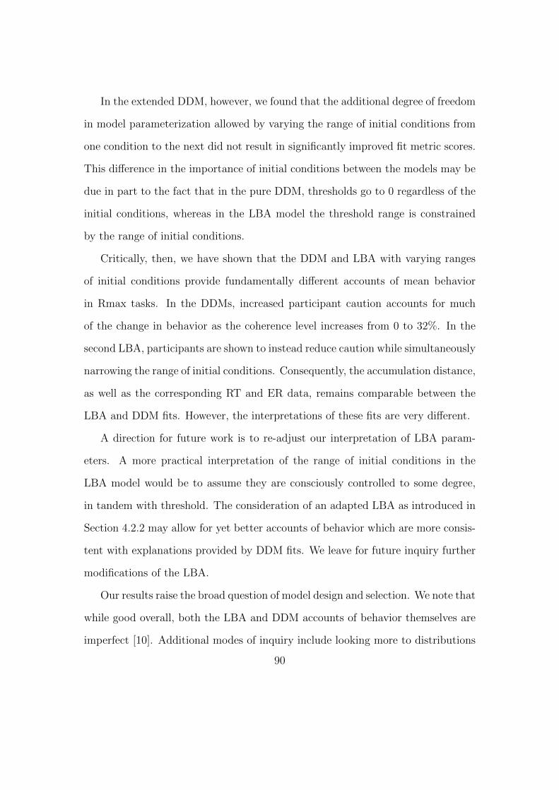
In the extended DDM, however, we found that the additional degree of freedom

in model parameterization allowed by varying the range of initial conditions from

one condition to the next did not result in significantly improved fit metric scores.

This difference in the importance of initial conditions between the models may be

due in part to the fact that in the pure DDM, thresholds go to 0 regardless of the

initial conditions, whereas in the LBA model the threshold range is constrained

by the range of initial conditions.

Critically, then, we have shown that the DDM and LBA with varying ranges

of initial conditions provide fundamentally different accounts of mean behavior

in Rmax tasks. In the DDMs, increased participant caution accounts for much

of the change in behavior as the coherence level increases from 0 to 32%. In the

second LBA, participants are shown to instead reduce caution while simultaneously

narrowing the range of initial conditions. Consequently, the accumulation distance,

as well as the corresponding RT and ER data, remains comparable between the

LBA and DDM fits. However, the interpretations of these fits are very different.

A direction for future work is to re-adjust our interpretation of LBA param-

eters. A more practical interpretation of the range of initial conditions in the

LBA model would be to assume they are consciously controlled to some degree,

in tandem with threshold. The consideration of an adapted LBA as introduced in

Section 4.2.2 may allow for yet better accounts of behavior which are more consis-

tent with explanations provided by DDM fits. We leave for future inquiry further

modifications of the LBA.

Our results raise the broad question of model design and selection. We note that

while good overall, both the LBA and DDM accounts of behavior themselves are

imperfect [10]. Additional modes of inquiry include looking more to distributions

90

of RTs for OPCs in addition to mean behavior. While normalized mean DTs are of

use when calculating theories of optimal performance, and using normalized mean

DTs allows for a unique OPC to gauge behavior, this nondimensional approach

precludes the use of numerous existing toolsets designed to describe distributions

of RT.

Additional numerical and theoretical analysis are also of interest. For example,

we wish to compare additional models such as the Leaky Competing Accumulator

Model as well as theoretically optimal Bayesian accounts of behavior with the

models presented in this chapter.

With our fits and analyses, we identified a key difference between the LBA and

DDM accounts of behavior. While the best LBA description of Rmax behavior

involved a decrease in variability in initial conditions coupled with a decrease in

caution as the stimulus coherence varies from low to high coherence, the best

DDM descriptions involved an increase in caution. In summary, the DDM and

LBA accounts of Rmax task behaviors provide highly descriptive but inconsistent

accounts of the behavior of the participants. The Rmax task paradigm provides a

fruitful tool for model comparison.

4.5 Appendix

Figures 4.10-4.16 show details of fits to individual participants for the five models,

averaged over all trials in sessions 10-13, for each given coherence.

Figures 4.10 and 4.11 show RTs and ERs versus coherence for the experimental

data, and as predicted by fits of the five models. Figure 4.13 shows the mean

normalized DTs versus ERs in comparison with the unique OPC for the pure

91

DDM. Finally, Figures 4.12, 4.14, and 4.15 show reward rates (RR), thresholds

(z), and initial condition variability (sx, or A) versus coherence for the model fits.

In each of the figures, participants are presented from left to right and top

to bottom based on closeness of behavior to that predicted by the OPC for the

pure DDM. Closeness of behavior is measured by the squares of the differences

between mean normalized DTs and normalized DTs lying on the OPC for each

participant. The participant with the smallest score, Subject 39, appears in the

upper left corner of each figure, and the participant with the largest score, Subject

17, appears in the lower right corner of each figure.

92

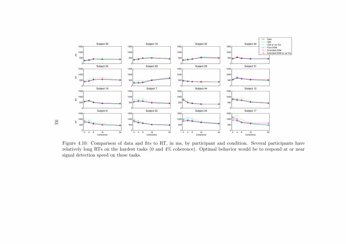
0

500

1000

1500

Subject 39

RT

0

500

1000

1500

Subject 16

0

500

1000

1500

Subject 32

0

500

1000

1500

Subject 30

0

500

1000

1500

Subject 20

RT

0

500

1000

1500

Subject 29

0

500

1000

1500

Subject 28

0

500

1000

1500

Subject 31

0

500

1000

1500

Subject 19

RT

0

500

1000

1500

Subject 7

0

500

1000

1500

Subject 44

0

500

1000

1500

Subject 12

0 4 8 16 320

500

1000

1500

Subject 6

RT

Coherence0 4 8 16 32

0

500

1000

1500

Subject 22

Coherence0 4 8 16 32

0

500

1000

1500

Subject 34

Coherence0 4 8 16 32

0

500

1000

1500

Subject 17

Coherence

Data

LBA

LBA w/ var ICs

Pure DDM

Extended DDM

Extended DDM w/ var ICs

Figure 4.10: Comparison of data and fits to RT, in ms, by participant and condition. Several participants haverelatively long RTs on the hardest tasks (0 and 4% coherence). Optimal behavior would be to respond at or nearsignal detection speed on these tasks.

93

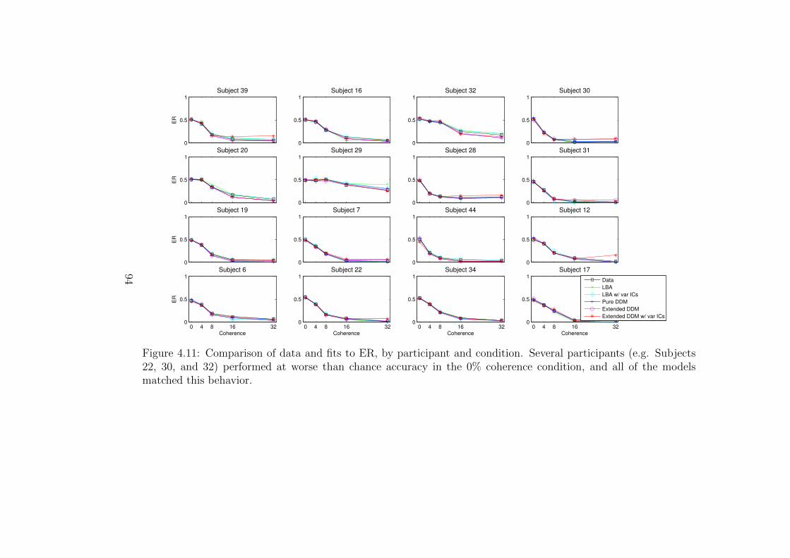
0

0.5

1

Subject 39

ER

0

0.5

1

Subject 16

0

0.5

1

Subject 32

0

0.5

1

Subject 30

0

0.5

1

Subject 20

ER

0

0.5

1

Subject 29

0

0.5

1

Subject 28

0

0.5

1

Subject 31

0

0.5

1

Subject 19

ER

0

0.5

1

Subject 7

0

0.5

1

Subject 44

0

0.5

1

Subject 12

0 4 8 16 320

0.5

1

Subject 6

ER

Coherence0 4 8 16 32

0

0.5

1

Subject 22

Coherence0 4 8 16 32

0

0.5

1

Subject 34

Coherence0 4 8 16 32

0

0.5

1

Subject 17

Coherence

Data

LBA

LBA w/ var ICs

Pure DDM

Extended DDM

Extended DDM w/ var ICs

Figure 4.11: Comparison of data and fits to ER, by participant and condition. Several participants (e.g. Subjects22, 30, and 32) performed at worse than chance accuracy in the 0% coherence condition, and all of the modelsmatched this behavior.

94

0

500

1000

Subject 39

RR

va

lue

0

500

1000

Subject 16

0

500

1000

Subject 32

0

500

1000

Subject 30

0

500

1000

Subject 20

RR

va

lue

0

500

1000

Subject 29

0

500

1000

Subject 28

0

500

1000

Subject 31

0

500

1000

Subject 19

RR

va

lue

0

500

1000

Subject 7

0

500

1000

Subject 44

0

500

1000

Subject 12

0 4 8 16 320

500

1000

Subject 6

RR

va

lue

Coherence0 4 8 16 32

0

500

1000

Subject 22

Coherence0 4 8 16 32

0

500

1000

Subject 34

Coherence0 4 8 16 32

0

500

1000

Subject 17

Coherence

Data

LBA

LBA w/ var ICs

Pure DDM

Extended DDM

Extended DDM w/ var ICs

Figure 4.12: Comparison of RR data (total rewards earned in Sessions 10-13) by participant and difficulty condition,in the data and the corresponding model predictions. Subject 29 had an unusual response curve and responded mostslowly in the relatively easy 32% coherence trials.

95

0

0.5

1

Subject 39

nD

T

0

0.5

1

Subject 16

0

0.5

1

Subject 32

0

0.5

1

Subject 30

0

0.5

1

Subject 20

nD

T

0

0.5

1

Subject 29

0

0.5

1

Subject 28

0

0.5

1

Subject 31

0

0.5

1

Subject 19

nD

T

0

0.5

1

Subject 7

0

0.5

1

Subject 44

0

0.5

1

Subject 12

0 0.5

0

0.5

1

Subject 6

nD

T

ER0 0.5

0

0.5

1

Subject 22

ER0 0.5

0

0.5

1

Subject 34

ER0 0.5

0

0.5

1

ER

Subject 17

LBA

Pure DDM

Extended DDM

LBA, Var. ICs

LBA Optimal

Extended DDM, Var. ICs

Figure 4.13: Model fits to mean normalized DT and ER data for each difficulty condition and participant. Some ofthe differences between LBA and DDM predictions here can be attributed to differences between the model estimatesof nondecision time.

96

0

0.1

0.2

Subject 39

z v

alu

e

0

0.1

0.2

Subject 16

0

0.1

0.2

Subject 32

0

0.1

0.2

Subject 30

0

0.1

0.2

Subject 20

z v

alu

e

0

0.1

0.2

Subject 29

0

0.1

0.2

Subject 28

0

0.1

0.2

Subject 31

0

0.1

0.2

Subject 19

z v

alu

e

0

0.1

0.2

Subject 7

0

0.1

0.2

Subject 44

0

0.1

0.2

Subject 12

0 4 8 16 320

0.1

0.2

Subject 6

z v

alu

e

Coherence0 4 8 16 32

0

0.1

0.2

Subject 22

Coherence0 4 8 16 32

0

0.1

0.2

Subject 34

Coherence0 4 8 16 32

0

0.1

0.2

Subject 17

Coherence

LBA

LBA w/ var ICs

Pure DDM

Extended DDM

Extended DDM w/ var ICs

Figure 4.14: Comparison of values of the caution or threshold parameter in the different model fits, by participantand condition. LBA threshold values have been scaled down by a factor of 5000, to fit on the same axis.

97

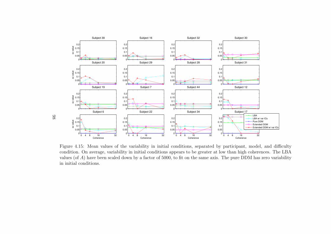
0

0.05

0.1

0.15

0.2

Subject 39

sx v

alu

e

0

0.05

0.1

0.15

0.2

Subject 16

0

0.05

0.1

0.15

0.2

Subject 32

0

0.05

0.1

0.15

0.2

Subject 30

0

0.05

0.1

0.15

0.2

Subject 20

sx v

alu

e

0

0.05

0.1

0.15

0.2

Subject 29

0

0.05

0.1

0.15

0.2

Subject 28

0

0.05

0.1

0.15

0.2

Subject 31

0

0.05

0.1

0.15

0.2

Subject 19

sx v

alu

e

0

0.05

0.1

0.15

0.2

Subject 7

0

0.05

0.1

0.15

0.2

Subject 44

0

0.05

0.1

0.15

0.2

Subject 12

0 4 8 16 320

0.05

0.1

0.15

0.2

Subject 6

sx v

alu

e

Coherence0 4 8 16 32

0

0.05

0.1

0.15

0.2

Subject 22

Coherence0 4 8 16 32

0

0.05

0.1

0.15

0.2

Subject 34

Coherence0 4 8 16 32

0

0.05

0.1

0.15

0.2

Subject 17

Coherence

LBA

LBA w/ var ICs

Pure DDM

Extended DDM

Extended DDM w/ var ICs

Figure 4.15: Mean values of the variability in initial conditions, separated by participant, model, and difficultycondition. On average, variability in initial conditions appears to be greater at low than high coherences. The LBAvalues (of A) have been scaled down by a factor of 5000, to fit on the same axis. The pure DDM has zero variabilityin initial conditions.

98

−0.5

0

0.5

1

1.5

2

Subject 39

µ v

alu

e

−0.5

0

0.5

1

1.5

2

Subject 16

−0.5

0

0.5

1

1.5

2

Subject 32

−0.5

0

0.5

1

1.5

2

Subject 30

−0.5

0

0.5

1

1.5

2

Subject 20

µ v

alu

e

−0.5

0

0.5

1

1.5

2

Subject 29

−0.5

0

0.5

1

1.5

2

Subject 28

−0.5

0

0.5

1

1.5

2

Subject 31

−0.5

0

0.5

1

1.5

2

Subject 19

µ v

alu

e

−0.5

0

0.5

1

1.5

2

Subject 7

−0.5

0

0.5

1

1.5

2

Subject 44

−0.5

0

0.5

1

1.5

2

Subject 12

0 4 8 16 32−0.5

0

0.5

1

1.5

2

Subject 6

µ v

alu

e

Coherence0 4 8 16 32

−0.5

0

0.5

1

1.5

2

Subject 22

Coherence0 4 8 16 32

−0.5

0

0.5

1

1.5

2

Subject 34

Coherence0 4 8 16 32

−0.5

0

0.5

1

1.5

2

Subject 17

Coherence

LBA

LBA w/ var ICs

Pure DDM

Extended DDM

Extended DDM w/ var ICs

Figure 4.16: Mean values of the drift parameter, µ, separated by participant, model, and coherence condition. Asexpected, drift magnitude increases monotonically with coherence. Note that LBA drift rate estimates have notbeen shifted, as was done for the subject-averaged data of Figure 4.9.

99

Chapter 5

Conclusion and Future Directions

In this thesis, we considered the dynamics of human performance in simple clas-

sification tasks. Motivated by the potential to better understand and support a

human operator, we studied human performance in several simple tasks. We re-

analyzed data from two previously published studies and performed one original

experiment to find new patterns in sequential decision tasks, and we developed

models to account for these patterns. Our primary findings are that:

• Sequential effects can be explained in part by post-error slowing.

We reconsidered prior experiments and models of sequential effects and

showed that in each of these experiments there was a significant post-error

slowing effect for which the existing models of sequential effects could not

account. By incorporating post-error adjustments to the threshold or cau-

tion parameter in our model, we were able to generate superior fits to both

post-error responses and to the sequential response dynamics. This analysis

is described in Chapter 2.

100

• Sequential effects are influenced by the relative likelihood of repe-

titions and alternations.

We analyzed data from an original study in which the likelihood of a given

stimulus being a repetition or alternation of the previous stimulus varied

between blocks of trials. We showed that the influence of a repetition or

alternation trial on behavior on that trial had strong effects on both RT and

ER. This work is described in Chapter 3.

• Reward maximization task performance allows us to differentiate

subjects and discriminate between models.

We reanalyzed data from a previous study [6] in which individuals earned a

fixed reward for each correct response and were instructed to optimize the

rate at which they would earn such rewards, and we compared fits of the pure

and extended DDMs as well as the LBA to subject performance on this task.

As in that study, we found that a portion of the subjects performed nearly

optimally. While average subjects could be modeled adequately by either

version of the DDM and the LBA, we found that the two models provide

fundamentally different accounts of behavior in Rmax tasks, with the DDM

predicting increases in caution and the second version of the LBA model

predicting relative decreases in caution. This work is described in Chapter

4.

101

5.1 Discussion

Our conclusions are the result of a careful analysis of three behavioral experi-

ments. The first experiment tasked subjects to classify a binary stimulus. Pre-

viously presented in [28], the task required subjects to identify which one of two

types of stimuli appear on a computer screen. The second task required motion

discrimination, using the moving dots paradigm with stimuli biased to show more

repetitions or alternations in each block of trials, in addition to the usual equally

probable case. We have previously presented the results of the second experiment

in [52]. The final experiment, reanalyzed from [6], again used equally probable as

opposed to biased random stimuli, also with the moving dots paradigm, but with

task difficulty levels varied by block and rewards provided for correct responses,

so that optimally performing subjects would need to tradeoff speed for accuracy

in order to maximize their reward rates.

Each analysis relied heavily upon the manipulation of a response threshold, or

caution parameter. In particular, we first considered in Chapters 2 and 3 reactive,

sequential adjustments to the threshold, with higher values after an incorrect re-

sponse and lowered values after a correct one. We then considered in Chapter 4

strategic overall adjustment of thresholds and ranges of initial conditions as diffi-

culty changes from one block of trials to the next. In each case our analysis allowed

us to identify differences between the predictions of various models and to suggest

which of a group of candidate models would be best suited to account for subject

behavior in a given data set.

Most critically, we identified new and powerful ways to discriminate between

models of simple two alternative forced choice RT tasks by studying predictions

102

of responses to sequences of stimuli and to rewarded tasks. In particular, in the

second and third chapters of this thesis, we considered combinations of factors in-

cluding post-error slowing, sequential effects in tasks with equally probable stimuli,

sequential effects for a task with a bias towards repetitions or alternations, and

sequential effects for correct and error trials. In the fourth chapter, we considered

reward maximization behavior at various task difficulty levels.

5.2 Future Work

In this thesis we considered separately the manipulation of stimulus sequence and

task difficulty; one interesting direction for future work is to study the interaction

of sequential effects and task difficulty. Our first experiment served as a con-

trol, in which stimulus sequence and task difficulty were held constant. We then

modulated the stimulus sequences in our second experiment so that repetitions or

alternations would be more likely. However, the interaction of stimulus sequence

and task difficulty and the combined influence of these factors on subject perfor-

mance is of interest for several reasons. Mechanistically, we expect these effects to

be modelled by a combination of reactive sequential threshold adjustments, and

possibly adjustments of other parameters, as described in Chapter 2, and strategic

overall mean threshold adjustments, as described in Chapter 4. Practically, we

expect interesting and nuanced interactions here, involving different time scales,

because sequential effects on their own have been shown to directly relate to se-

quence learning [115]. In addition, learning processes and behavior in the world

at large are understood to be driven by rewards and punishments [121, 45].

103

Specifically, we are interested in several additional directions which follow logi-

cally from the work presented in this thesis. In particular, we would like to further

extend the results of the study of sequential effects in Chapters 2 and 3 by con-

ducting and analyzing the results of a larger scale experiment with a range of task

difficulties, allowing us to study the resulting variability in processing times and

patterns for correct and incorrect responses. In addition, we would like to consider

and compare additional methods of model parameter adjustments, particularly in-

volving variation of the threshold parameter. In this work, we fit models in which

the threshold was either fixed or was allowed to increase or decrease by a fixed,

finite increment on each trial. Multiple studies have prescribed a trial-to-trial vari-

ability in the value of the threshold or allow the threshold to be randomly selected

from the distribution [93, 95]. However, to our knowledge, no prior studies have

systematically considered and compared alternative methods for threshold adjust-

ments (for example, gradually changing the rate of change of the threshold from

trial to trial, or “resetting” the threshold after a certain number of trials). We

would like to consider alternate methods of varying the response threshold from

trial to trial.

Finally, model comparison methods discussed in this thesis can be used to

differentiate between additional models not considered in this thesis, including

nonlinear models, such as the Leaky Competing Accumulator. In the context of

competing accumulator models, the different effects of varying initial condition

versus thresholds can be more carefully considered using methods discussed in

this paper.

We are also interested in exploring potential applications of this knowledge to

assist the human in human-in-the-loop tasks. For example, in tasks such as vehicle

104

navigation or various security monitoring activities, participants are expected to

be fully awake and aware, but are subject to fatigue and distraction. Patterns in

the reaction time of an individual, coupled with an estimate of his or her general

accuracy, could allow for the early identification and possible prevention of costly

errors. Such future projects can help validate our findings and more importantly,

they can provide deeper insight into the several areas of study covered by this

work, especially engineering and neuroscience.

105

Bibliography

[1] H. Akaike. A new look at the statistical model identification. AutomaticControl, IEEE Transactions on, 19(6):716–723, 1974.

[2] H. Akaike. Likelihood and the Bayes procedure. Trabajos de Estadıstica yde Investigacion Operativa, 31(1):143–166, 1980.

[3] H. Akaike. Likelihood of a model and information criteria. Journal of Econo-metrics, 16(1):3–14, 1981.

[4] R. Audley. Some observations on theories of choice reaction time: Tutorialreview. Academic Press New York, 1973.

[5] F. Balci. Personal Communication, June 2011.

[6] F. Balci, P. Simen, R. Niyogi, A. Saxe, J.A. Hughes, P. Holmes, and J.D.Cohen. Acquisition of decision making criteria: reward rate ultimately beatsaccuracy. Attention, Perception, & Psychophysics, 73(2):640–657, 2011.

[7] Y. Bar-Shalom, X.R. Li, T. Kirubarajan, and J. Wiley. Estimation withapplications to tracking and navigation. Wiley Online Library, 2001.

[8] P. Bertelson. Sequential redundancy and speed in a serial two-choice re-sponding task. Quarterly Journal of Experimental Psychology, 13:90–102,1961.

[9] R. Blake, M. Rizzo, and S. McEvoy. Aging and perception of visual formfrom temporal structure. Psychology and Aging, 23(1):181, 2008.

[10] R. Bogacz, E. Brown, J. Moehlis, P. Holmes, and J.D. Cohen. The physicsof optimal decision making: a formal analysis of models of performance intwo-alternative forced-choice tasks. Psychological Review, 113(4):700–765,2006.

106

[11] R. Bogacz, P.T. Hu, P.J. Holmes, and J.D. Cohen. Do humans produce thespeed-accuracy trade-off that maximizes reward rate? Quarterly Journal ofExperimental Psychology, 63(5):863–891, 2010.

[12] M.M. Botvinick, T.S. Braver, D.M. Barch, C.S. Carter, and J.D. Cohen.Conflict monitoring and cognitive control. Psychological Review, 108(3):624–652, 2001.

[13] B. Bouzy and T. Cazenave. Computer go: an AI oriented survey. ArtificialIntelligence, 132(1):39–103, 2001.

[14] D.H. Brainard. The psychophysics toolbox. Spatial Vision, 10(4):433–436,1997.

[15] N. Brewer and GA Smith. How normal and retarded individuals monitorand regulate speed and accuracy of responding in serial choice tasks. Journalof Experimental Psychology: General, 113(1):71, 1984.

[16] K.H. Britten, W.T. Newsome, M.N. Shadlen, S. Celebrini, J.A. Movshon,et al. A relationship between behavioral choice and the visual responses ofneurons in macaque MT. Visual Neuroscience, 13:87–100, 1996.

[17] K.H. Britten, M.N. Shadlen, W.T. Newsome, and J.A. Movshon. The anal-ysis of visual motion: a comparison of neuronal and psychophysical perfor-mance. Journal of Neuroscience, 12(12):4745–4765, 1992.

[18] K.H. Britten, M.N. Shadlen, W.T. Newsome, J.A. Movshon, et al. Responsesof neurons in macaque MT to stochastic motion signals. Visual Neuroscience,10:1157–1157, 1993.

[19] K.H. Brodersen, W.D. Penny, L.M. Harrison, J. Daunizeau, C.C. Ruff,E. Duzel, K.J. Friston, and K.E. Stephan. Integrated bayesian models oflearning and decision making for saccadic eye movements. Neural Networks,21(9):1247–1260, 2008.

[20] S.D. Brown and A. Heathcote. The simplest complete model of choice re-sponse time: Linear ballistic accumulation. Cognitive Psychology, 57(3):153–178, 2008.

[21] K.P. Burnham and D.R. Anderson. Model selection and multimodel infer-ence: a practical information-theoretic approach. Springer Verlag, New York,2002.

[22] J.R. Busemeyer and J.T. Townsend. Fundamental derivations from decisionfield theory. Mathematical Social Sciences, 23(3):255–282, 1992.

107

[23] L. Busse, A. Ayaz, N.T. Dhruv, S. Katzner, A.B. Saleem, M.L. Scholvinck,A.D. Zaharia, and M. Carandini. The detection of visual contrast in thebehaving mouse. Journal of Neuroscience, 31(31):11351–11361, 2011.

[24] M. Campbell, A.J. Hoane, and F. Hsu. Deep blue. Artificial Intelligence,134(1):57–83, 2002.

[25] E.J. Capaldi. Partial reinforcement: A hypothesis of sequential effects. Psy-chological Review, 73(5):459, 1966.

[26] R.H.S. Carpenter and M.L.L. Williams. Neural computation of log likelihoodin control of saccadic eye movements. Nature, 377(6544):59–62, 1995.

[27] H. Chernoff and EL Lehmann. The use of maximum likelihood estimatesin chi-square tests for goodness of fit. Annals of Mathematical Statistics,25(3):579–586, 1954.

[28] R.Y. Cho, L.E. Nystrom, E.T. Brown, A.D. Jones, T.S. Braver, P.J. Holmes,and J.D. Cohen. Mechanisms underlying dependencies of performance onstimulus history in a two-alternative forced-choice task. Cognitive, Affective,& Behavioral Neuroscience, 2(4):283–299, 2002.

[29] K.G. Coffman and A.M. Odlyzko. Internet growth: Is there a “moore’s law”for data traffic? In Handbook of Massive Data Sets. Citeseer, 2001.

[30] Jacob Cohen, Patricia Cohen, Stephen G. West, and Leona S. Aiken. Ap-plied Multiple Regression/Correlation Analysis for the Behavioral Sciences.Mahwah, NJ, 2003.

[31] T.F. Coleman and Y. Li. On the convergence of interior-reflective newtonmethods for nonlinear minimization subject to bounds. Mathematical Pro-gramming, 67(1):189–224, 1994.

[32] T.F. Coleman and Y. Li. An interior trust region approach for minimizationsubject to bounds. SIAM Journal on Optimization, 6(2):418–445, 1996.

[33] G.S. Corrado, L.P. Sugrue, H.S. Seung, and W.T. Newsome. Linear-nonlinear-poisson models of primate choice dynamics. Journal of the Ex-perimental Analysis of Behavior, 84(3):581, 2005.

[34] A. Cypher. Eager: Programming repetitive tasks by example. In Proceed-ings of the SIGCHI Conference on Human Factors in Computing Systems:Reaching Through Technology, pages 33–39. ACM, 1991.

108

[35] N. Dalal and B. Triggs. Histograms of oriented gradients for human de-tection. In Computer Society Conference on Computer Vision and PatternRecognition, volume 1, pages 886–893. IEEE, 2005.

[36] Department of Defense. Department of Defense Modeling and Simulation(M&S) Glossary, 5000.59m edition, 1998.

[37] T.A. Dingus and M.C. Hulse. Some human factors design issues and recom-mendations for automobile navigation information systems. TransportationResearch Part C: Emerging Technologies, 1(2):119–131, 1993.

[38] C. Donkin, L. Averell, S. Brown, and A. Heathcote. Getting more fromaccuracy and response time data: Methods for fitting the linear ballisticaccumulator. Behavior Research Methods, 41(4):1095–1110, 2009.

[39] C. Donkin, S. Brown, A. Heathcote, and E.J. Wagenmakers. Diffusion ver-sus linear ballistic accumulation: different models but the same conclusionsabout psychological processes? Psychonomic Bulletin & Review, 18(1):1–9,2011.

[40] C. Dudschig and I. Jentzsch. Speeding before and slowing after errors: Is itall just strategy? Brain Research, 1296:56–62, 2009.

[41] W. Feller. An Introduction to Probability Theory and its Applications. NewYork: Wiley, 1968.

[42] S. Feng, P. Holmes, A. Rorie, and W.T. Newsome. Can monkeys chooseoptimally when faced with noisy stimuli and unequal rewards? PLoS Com-putational Biology, 5(2), 2009.

[43] D.G. Ferrington, B.S. Nail, and M. Rowe. Human tactile detection thresh-olds: modification by inputs from specific tactile receptor classes. Journalof Physiology, 272(2):415–433, 1977.

[44] P.A. Frensch and C.S. Miner. Effects of presentation rate and individualdifferences in short-term memory capacity on an indirect measure of seriallearning. Memory & Cognition, 22(1):95–110, 1994.

[45] W.T. Fu and J.R. Anderson. Solving the credit assignment problem: Ex-plicit and implicit learning of action sequences with probabilistic outcomes.Psychological Research, 72(3):321–330, 2008.

[46] J. Gao, K.F. Wong-Lin, P. Holmes, P. Simen, and J.D. Cohen. Sequentialeffects in two-choice reaction time tasks: Decomposition and synthesis ofmechanisms. Neural Computation, 21(9):2407–2436, 2009.

109

[47] C.W. Gardiner. Handbook of Stochastic Methods for Physics, Chemistry,and the Natural Sciences. Springer-Verlag, Berlin, 1985.

[48] C.D. Gilbert and T.N. Wiesel. Receptive field dynamics in adult primaryvisual cortex. Nature, 356(6365):150–152, 1992.

[49] J.I. Gold, C.T. Law, P. Connolly, and S. Bennur. The relative influencesof priors and sensory evidence on an oculomotor decision variable duringperceptual learning. Journal of Neurophysiology, 100(5):2653, 2008.

[50] J.I. Gold and M.N. Shadlen. Representation of a perceptual decision indeveloping oculomotor commands. Nature, 404(6776):390–394, 2000.

[51] J.I. Gold and M.N. Shadlen. Neural computations that underlie decisionsabout sensory stimuli. Trends in Cognitive Sciences, 5(1):10–16, 2001.

[52] S. Goldfarb, K.F. Wong-Lin, M. Schwemmer, N.E. Leonard, and P. Holmes.Can post-error dynamics explain sequential reaction time patterns? Fron-tiers in Psychology, 3(213), 2012.

[53] K. Grill-Spector and R. Malach. The human visual cortex. Annual Reviewof Neuroscience, 27:649–677, 2004.

[54] A.C. Harvey. Forecasting, structural time series models and the KalmanFilter. Cambridge University Press, 1991.

[55] A. Heathcote, S. Brown, and D. Cousineau. QMPE: Estimating Lognor-mal, Wald, and Weibull RT distributions with a parameter-dependent lowerbound. Behavior Research Methods, 36(2):277–290, 2004.

[56] A. Hernandez, A. Zainos, and R. Romo. Neuronal correlates of sensorydiscrimination in the somatosensory cortex. Proceedings of the NationalAcademy of Sciences, 97(11):6191, 2000.

[57] S.A. Huettel, A.W. Song, and G. McCarthy. Decisions under uncertainty:probabilistic context influences activation of prefrontal and parietal cortices.Journal of Neuroscience, 25(13):3304–3311, 2005.

[58] A.C. Huk and M.N. Shadlen. Neural activity in macaque parietal cortexreflects temporal integration of visual motion signals during perceptual de-cision making. Journal of Neuroscience, 25(45):10420–10436, 2005.

[59] C.M. Hurvich and C.L. Tsai. Regression and time series model selection insmall samples. Biometrika, 76(2):297–307, 1989.

110

[60] B. Javidi. Image Recognition and Classification: Algorithms, Systems, andApplications, volume 78. CRC Press, 2002.

[61] I. Jentzsch and C. Dudschig. Why do we slow down after an error? mech-anisms underlying the effects of posterror slowing. Quarterly Journal ofExperimental Psychology, 62(2):209–218, 2009.

[62] I. Jentzsch and H. Leuthold. Response conflict determines sequential effectsin serial response time tasks with short response-stimulus intervals. Journalof Experimental Psychology: Human Perception and Performance, 31:731–748, 2005.

[63] I. Jentzsch, H. Leuthold, and R. Ulrich. Decomposing sources of responseslowing in the prp paradigm. Journal of Experimental Psychology: HumanPerception and Performance, 33(3):610, 2007.

[64] I. Jentzsch and W. Sommer. Sequence-sensitive subcomponents of P300:Topographical analyses and dipole source localization. Psychophysiology,38(4):607–621, 2001.

[65] I. Jentzsch and W. Sommer. Functional localization and mechanisms ofsequential effects in serial reaction time tasks. Perception & Psychophysics,64(7):1169, 2002.

[66] A.D. Jones, R.Y. Cho, L.E. Nystrom, J.D. Cohen, and T.S. Braver. A com-putational model of anterior cingulate function in speeded response tasks:Effects of frequency, sequence, and conflict. Cognitive, Affective, & Behav-ioral Neuroscience, 2(4):300–317, 2002.

[67] W.Q. Judge and A. Miller. Antecedents and outcomes of decision speed indifferent environmental contexts. Academy of Management Journal, pages449–463, 1991.

[68] W. Karwowski. International encyclopedia of ergonomics and human factors,volume 3. CRC, 2000.

[69] N.H. Kirby. Sequential effects in two-choice reaction time: Automatic fa-cilitation or subjective expectancy. Journal of Experimental Psychology,2(4):567–577, 1976.

[70] D. Laming. Autocorrelation of choice-reaction times. Acta Psychologica,43(5):381–412, 1979.

[71] D. Laming. Choice reaction performance following an error. Acta Psycho-logica, 43(3):199–224, 1979.

111

[72] D.R.J. Laming. Information Theory of Choice-Reaction Times. AcademicPress New York:, 1968.

[73] S.W. Link. The relative judgment theory of two choice response time. Journalof Mathematical Psychology, 12(1):114–135, 1975.

[74] S.W. Link and R.A. Heath. A sequential theory of psychological discrimina-tion. Psychometrika, 40(1):77–105, 1975.

[75] Y.S. Liu, A. Yu, and P. Holmes. Dynamical analysis of Bayesian inferencemodels for the Eriksen task. Neural Computation, 21(6):1520–1553, 2009.

[76] G.E. Moore et al. Cramming more components onto integrated circuits.Proceedings of the IEEE, 86(1):82–85, 1965.

[77] M. Muller. Computer go. Artificial Intelligence, 134(1):145–179, 2002.

[78] J. Nachmias. On the psychometric function for contrast detection. VisionResearch, 21(2):215–223, 1981.

[79] A. Nedic, D. Tomlin, P. Holmes, D.A. Prentice, and JD Cohen. A deci-sion task in a social context: Human experiments, models, and analyses ofbehavioral data. Proceedings of the IEEE, (99):1–21, 2011.

[80] M. Newborn and M. Newborn. Kasparov vs. Deep Blue: Computer chesscomes of age. Springer-Verlag New York, Inc., 1997.

[81] W.T. Newsome, K.H. Britten, J.A. Movshon, and M. Shadlen. Single neu-rons and the perception of visual motion. In Lam D.M.K. and C.D. Gilbert,editors, Neural mechanisms of visual perception, pages 171–198, Woodlands,TX, April 1989. Retina Research Foundation Symposium, Portfolio Publish-ing Co.

[82] W.T. Newsome and E.B. Pare. A selective impairment of motion perceptionfollowing lesions of the middle temporal visual area. Journal of Neuroscience,8(6):2201–2211, 1988.

[83] G.A. Orban. Imaging image processing in the human brain. Current Opinionin Neurology, 14(1):47, 2001.

[84] H. Pashler and G. Baylis. Procedural learning: 1. Locus of practice effectsin speeded choice tasks. Contract, 14(88-K):0281, 1991.

[85] H. Pashler and G. Baylis. Procedural learning: 2. Intertrial repetition effectsin speeded-choice tasks. Learning, Memory, 17(1):33–48, 1991.

112

[86] A.P. Prudnikov, Y.A. Brychkov, and O.I. Marichev. Integrals and Series.Vol. 1: Elementary Functions. New York: Gordon and Breach, 1986.

[87] P. Rabbitt and B. Rodgers. What does a man do after he makes an error?An analysis of response programming. Quarterly Journal of ExperimentalPsychology, 29(4):727–743, 1977.

[88] P. Rabbitt and S. Vyas. Processing a display even after you make a re-sponse to it. how perceptual errors can be corrected. Quarterly Journal ofExperimental Psychology, 33(3):223–239, 1981.

[89] P.M. Rabbitt. Errors and error correction in choice-response tasks. Journalof Experimental Psychology, 71(2):264–272, 1966.

[90] P.M. Rabbitt. Repetition effects and signal classification strategies in serialchoice-response tasks. The Quarterly Journal of Experimental Psychology,20(3):232, 1968.

[91] P.M. Rabbitt. Three kinds of error-signalling responses in a serial choicetask. Quarterly Journal of Experimental Psychology, 20(2):179, 1968.

[92] R. Ratcliff. A theory of memory retrieval. Psychological Review, 85(2):59,1978.

[93] R. Ratcliff. Group reaction time distributions and an analysis of distributionstatistics. Psychological Bulletin, 86(3):446, 1979.

[94] R. Ratcliff and G. McKoon. A retrieval theory of priming in memory. Psy-chological Review, 95(3):385, 1988.

[95] R. Ratcliff and G. McKoon. The diffusion decision model: Theory and datafor two-choice decision tasks. Neural Computation, 20(4):873–922, 2008.

[96] R. Ratcliff and J.N. Rouder. Modeling response times for two-choice deci-sions. Psychological Science, 9(5):347, 1998.

[97] R. Ratcliff and P.L. Smith. A comparison of sequential sampling models fortwo-choice reaction time. Psychological Review, 111(2):333, 2004.

[98] R. Ratcliff, D. Spieler, and G. McKoon. Explicitly modeling the effects ofaging on response time. Psychonomic Bulletin & Review, 7(1):1–25, 2000.

[99] R. Ratcliff, A. Thapar, P. Gomez, and G. McKoon. A diffusion model anal-ysis of the effects of aging in the lexical-decision task. Psychology and Aging,19(2):278, 2004.

113

[100] R. Ratcliff, A. Thapar, and G. McKoon. The effects of aging on reactiontime in a signal detection task. Psychology and Aging, 16(2):323, 2001.

[101] J. Reason. Human error: models and management. British Medical Journal,320(7237):768–770, 2000.

[102] R.J. Remington. Analysis of sequential effects on choice reaction times.Journal of Experimental Psychology, 82(2):250, 1969.

[103] J.L. Rodgers and W.A. Nicewander. Thirteen ways to look at the correlationcoefficient. American Statistician, 42(1):59–66, 1988.

[104] J.D. Schall and K.G. Thompson. Neural selection and control of visuallyguided eye movements. Annual Review of Neuroscience, 22(1):241–259, 1999.

[105] R.R. Schaller. Moore’s law: past, present and future. IEEE Spectrum,34(6):52–59, 1997.

[106] W. Schneider and R.M. Shiffrin. Controlled and automatic human informa-tion processing: I. detection, search, and attention. Psychological Review,84(1):1, 1977.

[107] G. Schwarz. Estimating the dimension of a model. Annals of Statistics,6(2):461–464, 1978.

[108] J.B. Sexton, E.J. Thomas, and R.L. Helmreich. Error, stress, and teamworkin medicine and aviation: cross sectional surveys. British Medical Journal,320(7237):745–749, 2000.

[109] P. Simen, J.D. Cohen, and P. Holmes. Rapid decision threshold modulationby reward rate in a neural network. Neural Networks, 19(8):1013–1026, 2006.

[110] P. Simen, D. Contreras, C. Buck, P. Hu, P. Holmes, and J.D. Cohen. Rewardrate optimization in two-alternative decision making: Empirical tests of the-oretical predictions. Journal of Experimental Psychology: Human Perceptionand Performance, 35(6):1865, 2009.

[111] D.G. Sinex, L.J. Burdette, and A.L. Pearlman. A psychophysical inves-tigation of spatial vision in the normal and reeler mutant mouse. VisionResearch, 19(8):853–857, 1979.

[112] A.F.M. Smith and D.J. Spiegelhalter. Bayes factors and choice criteria forlinear models. Journal of the Royal Statistical Society. Series B (Method-ological), 42(2):213–220, 1980.

114

[113] E. Soetens, L.C. Boer, and J.E. Hueting. Expectancy or automatic facilita-tion? separating sequential effects in two-choice reaction time. Journal ofExperimental Psychology: Human Perception and Performance, 11(5):598–616, 1985.

[114] E. Soetens, M. Deboeck, and J. Hueting. Automatic aftereffects in two-choicereaction time: A mathematical representation of some concepts. Journal ofExperimental Psychology: Human Perception and Performance, 10(4):581–598, 1984.

[115] E. Soetens, A. Melis, and W. Notebaert. Sequence learning and sequentialeffects. Psychological Research, 69(1):124–137, 2004.

[116] W. Sommer, H. Leuthold, and E. Soetens. Covert signs of expectancy inserial reaction time tasks revealed by event-related potentials. Perception &Psychophysics, 61(2):342–353, 1999.

[117] R.F. Stengel. Optimal Control and Estimation. Dover, 1994.

[118] A. Stewart, M. Cao, A. Nedic, D. Tomlin, and N. Ehrich Leonard. Towardshuman–robot teams: Model-based analysis of human decision making intwo-alternative choice tasks with social feedback. Proceedings of the IEEE,(99):1–25, 2012.

[119] M. Stone. Comments on model selection criteria of Akaike andSchwarz. Journal of the Royal Statistical Society. Series B (Methodologi-cal), 40(2):276–278, 1979.

[120] L.P. Sugrue, G.S. Corrado, and W.T. Newsome. Choosing the greater of twogoods: neural currencies for valuation and decision making. Nature ReviewsNeuroscience, 6(5):363–375, 2005.

[121] R.S. Sutton. Temporal credit assignment in reinforcement learning. PhDthesis, University of Massachusetts - Amherst, 1984.

[122] S.K. Talwar and G.L. Gerstein. Auditory frequency discrimination in thewhite rat. Hearing Research, 126(1-2):135–150, 1998.

[123] S. Thorpe, D. Fize, C. Marlot, et al. Speed of processing in the human visualsystem. Nature, 381(6582):520–522, 1996.

[124] C.T. Trevethan, A. Sahraie, L. Weiskrantz, et al. Form discrimination in acase of blindsight. Neuropsychologia, 45(9):2092–2103, 2007.

115

[125] F. Tuerlinckx. The efficient computation of the cumulative distribution andprobability density function in the diffusion model. Behavior Research Meth-ods, 36(4):702–716, 2004.

[126] M. Usher and J.L. McClelland. The time course of perceptual choice: Theleaky, competing accumulator model. Psychological Review, 108(3):550–592,2001.

[127] J. Vandekerckhove and F. Tuerlinckx. Fitting the ratcliff diffusion model toexperimental data. Psychonomic Bulletin & Review, 14(6):1011–1026, 2007.

[128] J. Vandekerckhove and F. Tuerlinckx. Diffusion model analysis with matlab:A dmat primer. Behavior Research Methods, 40(1):61, 2008.

[129] S. Venkataraman and RT Haftka. Structural optimization complexity: whathas moore’s law done for us? Structural and Multidisciplinary Optimization,28(6):375–387, 2004.

[130] K.R. Vervaeck and L.C. Boer. Sequential effects in two-choice reaction time:Subjective expectancy and automatic after-effect at short response-stimulusintervals. Acta Psychologica, 44(2):175–190, 1980.

[131] D.A. Wiegmann and S.A. Shappell. Human Error Analysis of CommercialAviation Accidents: Application of the Human Factors Analysis and Clas-sification System (HFACS). Aviation, Space, and Environmental Medicine,72(11), 2001.

[132] M.H. Wilder, M. Jones, and M.C. Mozer. Sequential effects reflect paral-lel learning of multiple environmental regularities. In Advances in NeuralInformation Processing Systems, volume 22, pages 2053–2061, 2010.

[133] A.J. Yu and J.D. Cohen. Sequential effects: Superstition or rational be-havior. In Advances in Neural Information Processing Systems, volume 21,pages 1873–1880, 2009.

[134] M. Zacksenhouse, R. Bogacz, and P. Holmes. Robust versus optimal strate-gies for two-alternative forced choice tasks. Journal of Mathematical Psy-chology, 54(2):230–246, 2010.

[135] J.C. Ziegler, C. Pech-Georgel, S. Dufau, and J. Grainger. Rapid process-ing of letters, digits and symbols: what purely visual-attentional deficit indevelopmental dyslexia? Developmental Science, 13(4):F8–F14, 2010.

116