mathematical physics-10-differential equations mathematica, one writes systems of equations in a...

Differential equations

Classification of differential equations

Differential equations (DEs) form the basis of physics. Every physical process evolving in time, within classical of quantum

mechanics, is described by a DE. Also many time independent physical situations are describable in terms of DEs. Examples

are problems of electrostatics and magnetostatics, theory of elasticity, stationary states in quantum mechanics.

Differential equations are equations for functions that contain their derivatives, such as

x@tD′ � f@t, [email protected] containing derivatives with respect to only one variable, as above, are called ordinary differential equations (ODEs). If

there are derivatives of multivariate functions over different variables in the equation, it is called partial differential equation

(PDE). In this chapter we study ODEs.

The highest order of derivatives in a DE defines the order of the DE. Above is the first-order DE. Higher-order DE can be

rewritten in a form of systems of first-order differential equations by considering lower-order derivatives as additional

functions. For instance, the second-order DE

x@tD′′ � f@t, x@tD′, x@tDDcan be rewritten as the system of two first-order DE

v@tD′ � f@t, v@tD, x@tDDx@tD′ == v@tD.

Combined order of a system of DEs is the sum of the orders of the individual equations (2 in the example above). Rewriting

a differential equation as a system of first-order DEs does not change the combined order.

DEs can be resolved or unresolved with respect to the highest derivative. Above are resolved DEs. Unresolved DEs can be

writen as F( t, x@tD′, x@tDL � 0 etc. In some cases these equations can be resolved with respect to the highest deriva-

tive (such as Hx@tD£L2 ã f[t, x[t]]), and in some cases not. It is difficult to find a physical model described by a DE non-

resolvable with respect to the highest derivative.

DEs can be linear and nonlinear with respect to derivatives and the function. An example of a linear ODE is

x@tD′′ + b x@tD′ + c x@tD == [email protected] the function on the right is called "inhomogeneous term". If the latter is zero, the linear ODE is callled "homogeneous".

ODEs with constant coefficients (as a and b above) can be solved analytically (see below). ODEs with variable coefficients

(functions of the independent variable) usually cannot be solved analytically. In some cases such ODEs define a special

function as their solution, if these equations are important. An important property of homogeneous linear equations is that if

x1@tD and x2@tD are solutions of the equation, then also C1 x1@tD + C2 x2@tD is a solution. The solution of an inhomogeneous

linear DE can be represented as a particular solution of this inhomogeneous equation plus a general solution of the corre-

sponding homogeneous equation that contains integration constants.

Vector differential equations

r@tD′ � f@t, r@tDDetc. are in fact systems of DEs for components

x@tD′ � fx@t, x@tD, y@tD, z@tDDy@tD′ � fy@t, x@tD, y@tD, z@tDDz@tD′ � fz@t, x@tD, y@tD, z@tDD.

In Mathematica, one writes systems of equations in a vector form by putting equations in a List.

Boundary conditions for differential equations

General solution of a system of DEs of a combined order N depends of N integration constants Cn. This situation is similar

with that of indefinite integrals. The integration constants have to be defined from the boundary conditions (BC) at the left

and right end of the interval, where the solution is considered. There should be exactly N boundary conditions to find N

integration constants.

If the independent variable is time, BC at the left end are called initial conditions. If the re are only initial conditions, the

problem is called evolutional and in general is solved simpler than a problem with BC at both ends.

As an example of an evolutional problem consider a particle moving in one dimension under the influence of a constant force

m x@tD′′ � F

where x@t] is particle's coordinate and m is its mass. First, DE is reduced to the system of first-order DEs

v@tD′ � F

m

x@tD′ � [email protected] the velocity and coordinate. Then the first equation is integrated directly, left and right parts

‡ �v@tD�t

�t = ‡ �v@tD = v@tD = ‡ F

m�t =

F

mt + C1

Then the resulting equation for x@t] is also integrated directly

‡ �x@tD�t

�t = ‡ �x@tD = x@tD = ‡ F

mt + C1 �t =

F

m

t2

2+ C1 t + C2

One can check that the solution

x@tD =F

m

t2

2+ C1 t + C2

satisfies the initial second-order DE. In fact, solution of this structure could be guessed. Now the boundary conditions are

found for the initial conditions

v@0D � v0, x@0D � x0.

This yields

C1 � v0, C2 � x0

and the well-known formulas for the motion with a constant acceleration a = F êmv@tD = at + v0

x@tD =a t2

2+ v0 t + x0.

Solution of differential equations with Mathematica

The Mathematica command for analytical solution of DEs is DSolve that takes both DEs and systems of DEs as its argument.

In the latter case, individual equations of a system have to be organized as a List. For instance, equation of motion in one

dimension for a body under the influence of a constant force is solved as

2 Mathematical_physics-10-Differential_equations.nb

DSolve@m x′′@tD � F, x@tD, tD

::x@tD →F t2

2 m+ C@1D + t C@2D>>

It can be used to define the solution of the DE as a function of time

xt@t_D = x@tD ê. DSolve@m x′′@tD � F, x, tD@@1DDF t2

2 m+ C@1D + t C@2D

Let us solve this equation again formulating it as a system of two first-order DEs

sol = DSolve@8m v′@tD � F, x′@tD � v@tD<, 8x@tD, v@tD<, tD

::v@tD →F t

m+ C@1D, x@tD →

F t2

2 m+ t C@1D + C@2D>>

Differential equations can be solved together with boundary conditions:

sol = DSolve@8m v′@tD � F, x′@tD � v@tD, x@0D � x0, v@0D � v0<, 8x@tD, v@tD<, tD êê Expand

::v@tD →F t

m+ v0, x@tD →

F t2

2 m+ t v0 + x0>>

Again, the time-dependent solution is defined as

xt@t_D = x@tD ê. sol@@1DDvt@t_D = v@tD ê. sol@@1DD

F t2

2 m+ t v0 + x0

F t

m+ v0

Let us now solve the equation of projectile motion in the x - y plane in the vector form. To make the vector DE solvable by

Mathematica, we first have to convert the equation for the vector (list) to a list of equations with Thread.

FVec = 8−m g, 0<; RVec@t_D = 8z@tD, x@tD<;DSolve@Thread@m RVec′′@tD � FVecD, RVec@tD, tD

::z@tD → −g t2

2+ C@1D + t C@2D, x@tD → C@3D + t C@4D>>

Numerical solution of DEs in Mathematica is done by NDSolve that we will consider below

Analytical solution of differential equations

Only DEs of special kinds can be solved analytically. No general analytical method of solution of DEs exists. Below we will

consider some cases in which DEs can be solved analytically

ü Separation of variables

If a first-order DE has a form

x@tD′ � g@xD f@tD

Mathematical_physics-10-Differential_equations.nb 3

one can integrate this DE directly after division by g@x]

‡ 1

g@xD�x@tD�t

�t = ‡ �x

g@xD � ‡ f@tD �t.

One can see that on the left there is only x and on the right there is only t. One can see it even clearer if one formally rewrites

the initial equation in the form

�x

g@xD = f@tD �t

before the integration. This is why this situation is called "separation of variables".

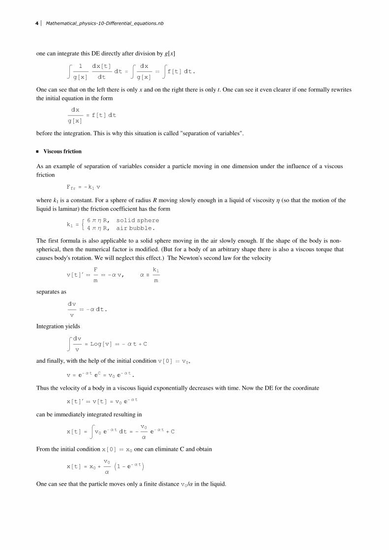
ü Viscous friction

As an example of separation of variables consider a particle moving in one dimension under the influence of a viscous

friction

Ffr = −k1 v

where k1 is a constant. For a sphere of radius R moving slowly enough in a liquid of viscosity h (so that the motion of the

liquid is laminar) the friction coefficient has the form

k1 = µ 6 π η R, solid sphere

4 π η R, air bubble.

The first formula is also applicable to a solid sphere moving in the air slowly enough. If the shape of the body is non-

spherical, then the numerical factor is modified. (But for a body of an arbitrary shape there is also a viscous torque that

causes body's rotation. We will neglect this effect.) The Newton's second law for the velocity

v@tD′ � F

m� −α v, α ≡

k1

m

separates as

�v

v� −α �t.

Integration yields

‡ �v

v= Log@vD � − α t + C

and finally, with the help of the initial condition v@0D � v0,

v = �− α t �C = v0 �− α t.

Thus the velocity of a body in a viscous liquid exponentially decreases with time. Now the DE for the coordinate

x@tD′ � v@tD = v0 �− α t

can be immediately integrated resulting in

x@tD = ‡ v0 �− α t �t = −v0

α�− α t + C

From the initial condition x@0D � x0 one can eliminate C and obtain

x@tD = x0 +v0

αI1 − �− α tM

One can see that the particle moves only a finite distance v0/a in the liquid.


Media resistance at high speeds

Resistance (friction) acting on a body fast moving in a liquid or in the air does not depend on the viscosity and is turbulent.

The corresponding friction force is impossible to obtain exactly but qualitative arguments and dimensional estimations yield

Ffr = −k2 v2,

where

k2 =1

2ρSγ

r being the density of the liquid, S being the cross-section of the body, and g being a numerical factor. This friction force can

be understood as the Bernoulli pressure P =1

2rv2 multiplied by the cross-section

S, plus a numerical factor g that is difficult to find : Ffr = gPS.

In this case the DE for the velocity is nonlinear

v@tD′ � −α2 v2, α2 ≡

k2

m

but still it can be solved by the separation of variables

�v

v2� −α2 �t

and then

‡ �v

v2=−1

v� − α2 t + C

that is, with the help of the boundary condition,

v@tD =1

α2 t + 1 ê v0It is noteworthy that at long times the velocity v does not depend on the initial velocity v0, so that the system forgets the

initial condition. This solution, as well as the expression for the friction force, is valid for v > 0.

Time dependence of the coordinate x@tD is obtained by the integration of the velocity

x@tD = ‡ v@tD �t = ‡ 1

α2 t + 1 ê v0 �t =1

α2LogBα2 t + 1

v0

F + C

From the initial condition x@0D � x0 one can eliminate C and obtain

x@tD = x0 +1

α2LogB

α2 t +1

v0

1

v0

F = x0 +1

α2Log@1 + v0 α2 tD.

Here x@t] increases infinitely but logarithmically slow at long times. However, at long times the speed becomes small and one

has to switch to the viscous friction force above. The crossover between the two different expressions for the friction force

should be at the speed at which both friction forces are comparable.

ü Using an integration factor

In some cases one can find a function to multiply by the differential equation, after which the left part containing the

unknown function becomes a derivative. In this case one can integrate the equation one time and solve or simplify the

problem. Finding an integration factor, if it is possible, is a matter of luck and skill.


Energy conservation

The most prominent example of using an integrating factor in physics is probably the derivation of the energy conservation

law from the equation of motion of conservative systems. Consider a point body under the action of a conservative (potential)

force

m r′′ � F@rD = −∂U@rD∂r

,

Dot-multiplying this DE by the integrating factor r′ and using the chain rule for differentiation, one can bring this equation

into the form of time derivatives on the right and on the left

m r′′ ⋅ r′ = m1

2Ir′2M′ � −

∂U@rD∂r

⋅ r′ = −U′@rD

Integrating this equation over time and substituting r′ = v, one obtains the energy conservation law

m v2

2+ U@rD � E,

where the conserved total energy E arises as an integration constant. For a motion in one dimension the energy conservation

law can be used to completely solve the problem. Solving the equation

m x′2

2+ U@xD � E,

for x′, one obtains the first-order DE

x′ � ±2 HE − U@xDL

m.

In this DE the variables separate and it can be integrated as

‡ 1

E − U@xD�x � ±

2

mt,

so that the problem reduces to the evaluation of the integral on the left. After that one has to find x@tD from a nonlinear

equation.

In multi-dimensional cases, the energy conservation law alone is insufficient to define the motion because it is one equation

containing more then one unknown function: x@tD, y@tD, etc., an underdetermined problem.

As an illustration consider a pendulum of mass m and length L described by the angle f (measured from the vertical down

direction) as the dynamical variable and having the energy

E =m v2

2+ mgh =

mL2 φ′2

2+ mgL H1 − Cos@φDL.

The equation of motion of the pendulum is

φ′′ + ω02 Sin@φD � 0, ω0 ≡

g

L.

Instead of solving this equation, one can use its one-time-integrated form following from the energy conservation law

E = const:

φ′ � ±2 HE − U@φDL

mL2= ±

2 HE − mgL H1 − Cos@φDLLmL2

.


This equation can be integrated by separation of variables

‡ 1

E − mgL H1 − Cos@φDL�φ � ±

2

mL2t.

The pendulum has turning points where its kinetic energy turns to zero and the sign in front of the square root changes sign.

Let us call the corresponding angle fmax. It depends on E and can be found from the equation

E � mgL H1 − Cos@φmaxD.In the sequel we will use fmax as the measure of pendulum's energy. A quarter of the pendulum's period T corresponds to its

motion from f = 0 to f = fmax. Thus the period can be found from

‡0

φmax 1

mgL HCos@φD − Cos@φmaxDL�φ =

2

mL2

T

4,

that is,

T = 23ê2L

g‡0

φmax 1

Cos@φD − Cos@φmaxD�φ.

that is,

T@φmax_D =

23ê2L

gIntegrateB 1

Cos@φD − Cos@φmaxD, 8φ, 0, φmax<, Assumptions → Cos@φmaxD < 1F

4 2L

gEllipticFB φmax

2, CscA φmax

2E2F

1 − Cos@φmaxDThis is a pretty complicated expression and Mathematica cannot simplify it. The plot

PlotB 1

2 πT@φmaxD ê. 8L → 1, g → 1<, 8φmax, 0, π<F

0.5 1.0 1.5 2.0 2.5 3.0

1.2

1.4

1.6

1.8

2.0

2.2

2.4

shows that for fmax` 1 the period approaches the known result

T = 2 πL

g.


Indeed,

Limit@T@φmaxD, 8φmax → 0<D@@1DD

2L

gπ

However, Mathematica produces a wrong series expansion of the result at fmax` 1:

Series@T@φmaxD, 8φmax, 0, 3<D

149L

g

30+

67

240

L

gφmax2 + O@φmaxD4

There are also glitches in plotting. All this underscores the importance of analytical work. One can put the result in a much

better shape rewriting it as

T = 2L

g‡0

φmax 1

SinA φmax

2E2 − SinA φ

2E2

�φ

using the new integration variable x defined by

Sin@ξD =SinA φ

2E

SinA φmax

2E.

The integral is transformed as follows

T = 2L

g‡0

πê2 1

SinA φmax

2E2 − SinA φmax

2E2 Sin@ξD2

�φ

�ξ�ξ =

2L

g‡0

πê2 1

SinA φmax

2E Cos@ξD

2 Cos@ξD SinA φmax

2E

CosA φ

2E

�ξ

Now with the help of

CosB φ2F = 1 − SinBφ

2F2

= 1 − SinB φmax2

F2

Sin@ξD2

one finally obtains

T = 4L

g‡0

πê2 �ξ

1 − SinA φmax

2E2 Sin@ξD2

= 4L

gKBSinB φmax

2F2

F,

where

K@mD = ‡0

πê2 �ξ

1 − m Sin@ξD2


is the elliptic intergal of the first kind. In this more transparent representation, one can easily see what is the period at small

amplitudes by expanding the integrand in small φmax. Using H1 - xL-1ê2> 1 + x ê2 one easily obtains

T > 4L

g‡0

πê21 +

1

2SinBφmax

2F2

Sin@ξD2 �ξ =

2 πL

g1 +

1

4SinBφmax

2F2

> 2 πL

g1 +

1

16φmax2 .

Let us plot this result

T@φmax_D = 4L

gEllipticKBSinB φmax

2F2

F

PlotB 1


4L

gEllipticKBSinB φmax

2F2

F

0.5 1.0 1.5 2.0 2.5 3.0

1.5

2.0

2.5

the same as above but a more accurate plot.

Mathematica yields


T@φmax_D = 4L

g‡0

πê2 ξ

1 − SinA φmax

2E2 Sin@ξD2

PlotB 1


4L

gEllipticKB−TanA φmax

2E2F

CosA φmax

2E2

0.5 1.0 1.5 2.0 2.5 3.0

1.5

2.0

2.5

again a different but equivalent analytical expression. The series expansion of the result has the form

Series@T@φmaxD, 8φmax, 0, 3<D

2L

gπ +

1

8

L

gπ φmax

2 + O@φmaxD4

now a correct expression.

ü Viscous friction with a constant force

As another example let us consider a particle moving in one dimension under the influence of the viscous friction and a time-

dependent force F@tD. The equation for the velocity has the form

v@tD′ � −α v@tD + f@tD, f@tD ≡F@tDm

with the positive direction of the x-axis along the force F. If the force is time-independent, the variables separate,

�v

−α v + f� �t

and the DE can be solved in this way. However, for the time-dependent force separation of variables does not occur. In tis

case, fortunately, one can find an integration factor that solves the problem. It is convenient to move the v-dependent term to

the left,

v@tD′ + α v@tD � f.

Now, multiplication of this DE by the integration factor �α t makes the left part a derivative:

�α t Hv@tD′ + α v@tDL = ∂tI�α t v@tDM � �α t f@tD,


so that the equation can be integrated as

�α t v@tD = ‡ �α t f@tD �t.In particular, for a time-independent force such as gravity the integral can be immediately done

�α t v@tD =1

α�α t f + C.

The solution is

v@tD =f

α+ �−α t C = v0 �

−α t +f

αI1 − �−α tM,

where the integration constant C was obtained from the boundary condition. Asymptotically at large times, the particle

forgets its initial velocity and takes the stationary velocity value v¶ =f

a. This result can be obtained directly from the

original DE setting v@tD′fl 0. After v[t] has been found, one can straighforwardly find v@t] by integration.

Non-evolutionary boundary conditions: Shooting

If boundary conditions are set at both sides of the interval of the independent variable, there is a little difference with the

case of BCs on one side if there is a general analytical solution of the DE. As before, integration constants are determined

from the BC after the general solution is obtained. If, however the DE can only be solved numerically, there is a big differ-

ence. DEs of the evolution type (all BCs on the left) are solved moving from the left to right along the trajectory that is

uniquely defined by the BCs on the left. If BCs are set at both ends of the interval, one cannot immediately find the trajectory

because BCs on the left do not contain the whole information about it. There is a freedom in the trajectory that is used to

satisfy the BCs on the right end. Numerically one can calculate trial trajectories and then choose those that satisfy the BCs on

the right. Of course, this procedure is more complicated and time consuming than solving evolution equations. Because the

first idea of such type of a problem is hitting a target at the right end of the interval, this class of problems and the method of

their solution outlined above is called shooting.

ü BCs on both ends: Free straight motion

As an example, suppose a body moves straight with no forces applied and was t = t0 at x = x0. At t = t1 > t0 the body should

be at x = x1. Find the motion of the body. The solution of the differential equation

x′′@tD � 0

is

x@tD = C1 t + C2

and the boundary conditions are

x@t0D � x0, x@t1D � x1

This yields the integration constants

C1 =x1 − x0

t1 − t0,

C2 = x0 − C1 t0 =x0 Ht1 − t0L − Hx1 − x0L t0

t1 − t0=x0 t1 − x1 t0

t1 − t0,

Obviously C1 = v, the constant velocity. This velocity is not given as the inital condition but follows from both boundary

conditions.


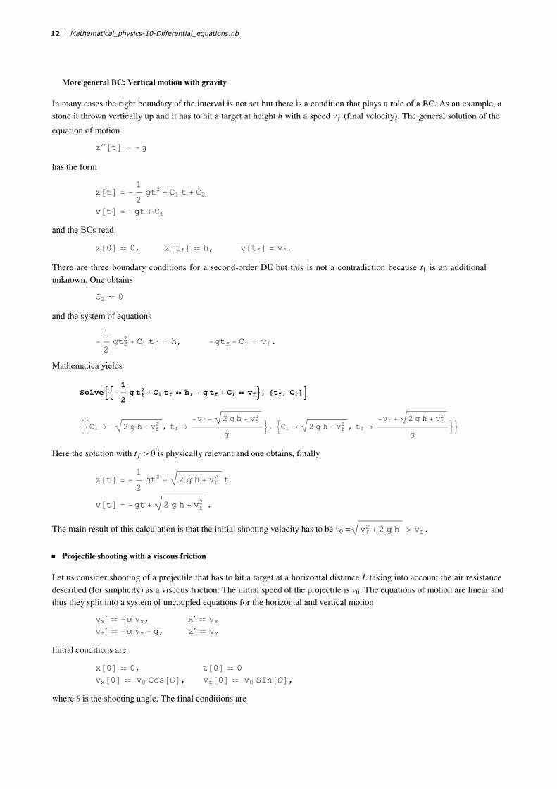
More general BC: Vertical motion with gravity

In many cases the right boundary of the interval is not set but there is a condition that plays a role of a BC. As an example, a

stone it thrown vertically up and it has to hit a target at height h with a speed v f (final velocity). The general solution of the

equation of motion

z′′@tD � −g

has the form

z@tD = −1

2gt2 + C1 t + C2

v@tD = −gt + C1

and the BCs read

z@0D � 0, z@tfD � h, v@tfD = vf.

There are three boundary conditions for a second-order DE but this is not a contradiction because t1 is an additional

unknown. One obtains

C2 � 0

and the system of equations

−1

2gtf

2 + C1 tf � h, −gtf + C1 � vf.

Mathematica yields

SolveB:− 1

2g tf

2 + C1 tf � h, −g tf + C1 � vf>, 8tf, C1<F

::C1 → − 2 g h + vf2 , tf →

−vf − 2 g h + vf2

g>, :C1 → 2 g h + vf

2 , tf →−vf + 2 g h + vf

2

g>>

Here the solution with t f > 0 is physically relevant and one obtains, finally

z@tD = −1

2gt2 + 2 g h + vf

2 t

v@tD = −gt + 2 g h + vf2 .

The main result of this calculation is that the initial shooting velocity has to be v0 = vf2 + 2 g h > vf.

ü Projectile shooting with a viscous friction

Let us consider shooting of a projectile that has to hit a target at a horizontal distance L taking into account the air resistance

described (for simplicity) as a viscous friction. The initial speed of the projectile is v0. The equations of motion are linear and

thus they split into a system of uncoupled equations for the horizontal and vertical motion

vx′ � −α vx, x′ � vx

vz′ � −α vz − g, z′ � vz

Initial conditions are

x@0D � 0, z@0D � 0

vx@0D � v0 Cos@θD, vz@0D � v0 Sin@θD,where q is the shooting angle. The final conditions are


x@tfD � L, z@tfD � 0

Solution of the system of DEs above contains four integration constants, and also there are unknown t f and q. For this we

have six boundary conditions, so that the problem is well determined. Solving equations for the velocity components as

above, one obtains

vx@tD = v0 Cos@θD �−α tvz@tD = v0 Sin@θD �−α t − g

αI1 − �−α tM

Integrating these equations yield

x@tD = ‡ v0 Cos@θD �−α t �t = −v0 Cos@θD �−α t

α+ Cx

z@tD = ‡ v0 Sin@θD �−α t − g

αI1 − �−α tM �t = −v0 Sin@θD �−α t

α−g

αt +

�−α t

α+ Cz

Finding the integration constants from the initial conditions one obtains

x@tD = v0 Cos@θD 1 − �−α t

α

z@tD = v0 Sin@θD 1 − �−α t

α−g

αt −

1 − �−α t

α= v0 Sin@θD + g

α

1 − �−α t

α−g

αt

It remains now to find t f and q from the final conditions above, that is

v0 Cos@θD 1 − �−α tf

α� L

v0 Sin@θD + g

α

1 − �−α tf

α−g

αtf � 0.

Eliminating the t f combination with the help of the first equation, one obtains

α

gv0 Sin@θD + 1 L

v0 Cos@θD � tf.

Substituting this result into the first equation, one obtains the transcedental equation for the shooting angle

v0 Cos@θD 1

α1 − ExpB−α α

gv0 Sin@θD + 1 L

v0 Cos@θDF − L � 0

In reality, the air resistance is small, thus this equation can be simplified by expansion at small a

NormalBSeriesBv0 Cos@θD1

α1 − ExpB−α α

gv0 Sin@θD + 1

L

v0 Cos@θDF − L, 8α, 0, 2<FF

α −L2 Sec@θD

2 v0

+L Sin@θD v0

g+ α2

L3 Sec@θD26 v0

2−L2 Tan@θD

g

Simplifying this, one obtains

SimplifyB% 2 g Cos@θDα v0 L

F

Sin@2 θD + g L2 α Sec@θD3 v0

3−g L

v02−2 L α Sin@θD

v0

thus for small a the equation has the form


Sin@2 θD − g L

v02−

αL

v0 Cos@θD Sin@2 θD − g L

3 v02

� 0

Setting a = 0 one recovers the well known result

Sin@2 θD =g L

v02

that yields two values of q corresponding to the high and low trajectories. The target can be hit only if v02¥gL. The final form

of the solution is

θ = ϑ1 =1

2ArcSinBg L

v02F <

π

4, θ = ϑ2 =

1

2π − ArcSinBg L

v02F >

π

4

Let us plot the trajectories with and without the air resistance


Parameters = 8g → 1., L → 1, v0 → 1.1, α → 0.05<;ϑ1 =

1

2ArcSinB g L

v02F ê. Parameters ; ϑ1

180

π

ϑ2 =1

2π − ArcSinB g L

v02F ê. Parameters ; ϑ2

180

π

x0@t_, θ_D := v0 Cos@θD t;z0@t_, θ_D := −

1

2g t2 + v0 Sin@θD t; H∗ Without air resistance ∗L

x@t_, θ_D := v0 Cos@θD1 − �−α t

α;

z@t_, θ_D := v0 Sin@θD +g

α

1 − �−α t

α−g

αt; H∗ With air resistance ∗L

ShowBParametricPlotB8x0@t, ϑ2D, z0@t, ϑ2D< ê. Parameters,

:t, 0,L

v0 Cos@ϑ2Dê. Parameters>, PlotStyle → 8Red, Dashed<F,

ParametricPlotB8x0@t, ϑ1D, z0@t, ϑ1D< ê. Parameters,

:t, 0,L

v0 Cos@ϑ1Dê. Parameters>, PlotStyle → 8Blue, Dashed<F,

ParametricPlotB8x@t, ϑ2D, z@t, ϑ2D< ê. Parameters,

:t, 0,L

v0 Cos@ϑ2Dê. Parameters>, PlotStyle → 8Red<F,


:t, 0,L

v0 Cos@ϑ1Dê. Parameters>, PlotStyle → 8Blue<F

F27.8677

62.1323

0.2 0.4 0.6 0.8 1.0

0.1

0.2

0.3

0.4

One can see that the high trajectory is more sensitive to the air resistance because the time and exposure to the resistance is

longer. In fact, the model of the viscous friction is not good for real shooting because in assumes small speeds whereas the

actual speeds are high. A better mathematical model includes the v2 damping but in this case the equations of motion are

nonlinear and cannot be solved analytically.


Let us now obtain the correction to the shooting angle due to the air resistance. Search for the solution in the form with

corrections linear in small a:

θ = θi = ϑi + δθi, i = 1, 2, †δθi§ ` 1

Inserting this into the equation, using

Sin@2 θD = Sin@2 Hϑi + δθiLD > Sin@2 ϑiD + 2 Cos@2 ϑiD δθiand keeping only linear-a terms in the equation, one obtains

2 Cos@2 ϑiD δθi − αL

v0 Cos@ϑiD Sin@2 ϑiD − g L

3 v02

� 0

or,

δθi =αL

v0 Cos@2 ϑiD Cos@ϑiDg L

3 v02.

This formula gives the corrections to the no-resustance formula for the air resistance. For the low trajectory Cos@2 ϑ1D>0

and one has to aim higher that is intuitively clear. For the high trajectory Cos@2 ϑ2D<0 and one has to aim lower. For the

maximal-distance shot, ϑ1=ϑ2=p/4, one has Cos@2 ϑ2D=0 and the formula above fails. In this case one cannot hit the target

at all because of the air resistance.

Let us plot the trajectories with and without the air resistance correction


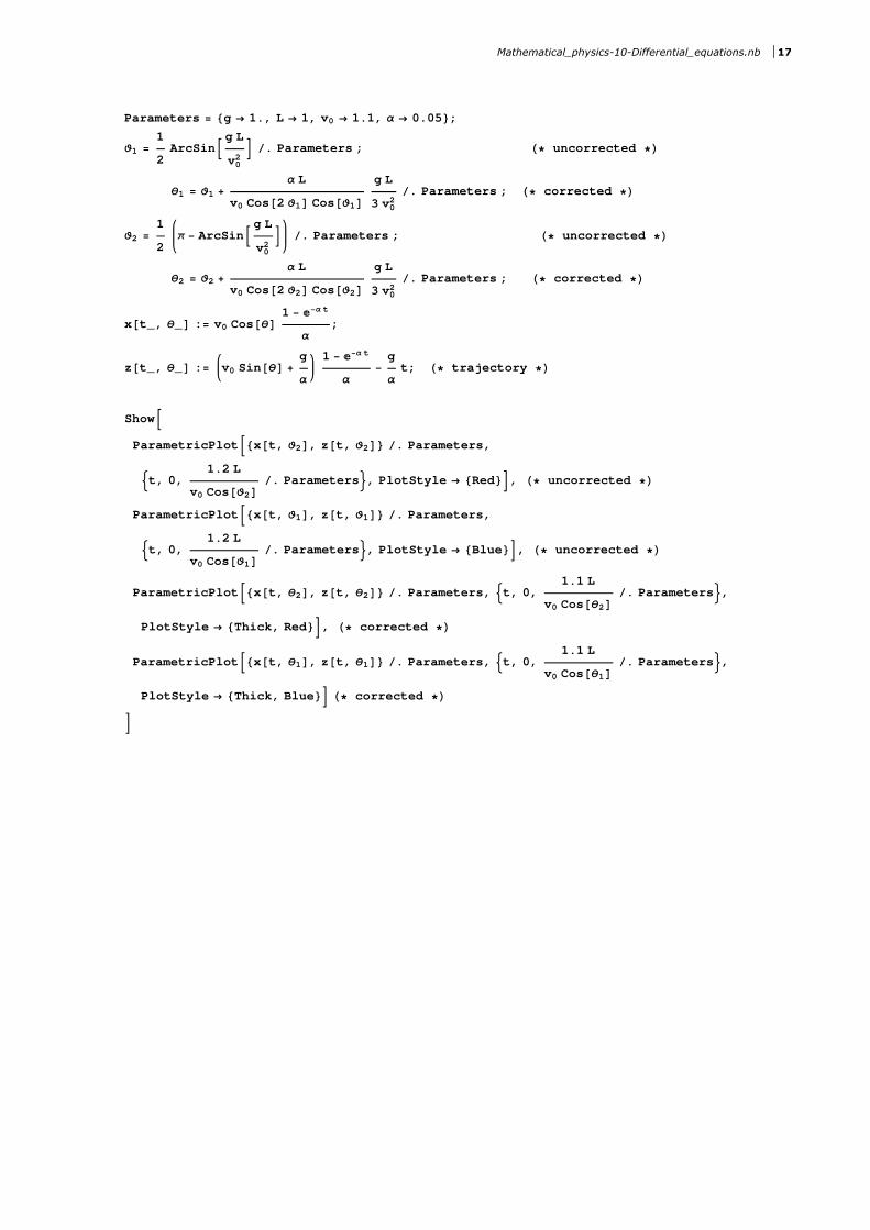
Parameters = 8g → 1., L → 1, v0 → 1.1, α → 0.05<;ϑ1 =

1

2ArcSinB g L

v02F ê. Parameters ; H∗ uncorrected ∗L

θ1 = ϑ1 +α L

v0 Cos@2 ϑ1D Cos@ϑ1Dg L

3 v02

ê. Parameters ; H∗ corrected ∗L

ϑ2 =1

2π − ArcSinB g L

v02F ê. Parameters ; H∗ uncorrected ∗L

θ2 = ϑ2 +α L

v0 Cos@2 ϑ2D Cos@ϑ2Dg L

3 v02

ê. Parameters ; H∗ corrected ∗L

x@t_, θ_D := v0 Cos@θD1 − �−α t

α;

z@t_, θ_D := v0 Sin@θD +g

α

1 − �−α t

α−g

αt; H∗ trajectory ∗L

ShowBParametricPlotB8x@t, ϑ2D, z@t, ϑ2D< ê. Parameters,

:t, 0,1.2 L

v0 Cos@ϑ2Dê. Parameters>, PlotStyle → 8Red<F, H∗ uncorrected ∗L


:t, 0,1.2 L

v0 Cos@ϑ1Dê. Parameters>, PlotStyle → 8Blue<F, H∗ uncorrected ∗L

ParametricPlotB8x@t, θ2D, z@t, θ2D< ê. Parameters, :t, 0,1.1 L

v0 Cos@θ2Dê. Parameters>,

PlotStyle → 8Thick, Red<F, H∗ corrected ∗L

ParametricPlotB8x@t, θ1D, z@t, θ1D< ê. Parameters, :t, 0,1.1 L

v0 Cos@θ1Dê. Parameters>,

PlotStyle → 8Thick, Blue<F H∗ corrected ∗LF


0.2 0.4 0.6 0.8 1.0

-0.4

-0.2

0.2

0.4

The target is almost hit. Note that the correcion due to the air resistance has been calculated approximately!

ü Linear DEs with constant coefficients

Linear DEs (and systems of DEs) with constant coefficients is probably the most important class of DEs. The solution of

homogeneous equations can be searched in the form

x@tD = C‰lt

that reduces the DE to an algebraic equation.

ü Viscous friction

For instance, the solution of the equation of motion of a body with a viscous friction

v′@tD + α v@tD � 0

can be searched in the form v@tD = C‰lt. Substituting this into the equation, one obtains the equation for l

Cλ�λt + αC�λt = C�λt Hλ + αL � 0 .

Since we are looking for a nontrivial solution with C ∫ 0, this equation yields l = -a. Of course, this simple equation can be

solved by other methods as well.

ü Harmonic oscillator

Let us consider the equation of one-dimensional motion of a body on a spring providing the restoring force F = -k x

mx′′@tD � F@xD = −kx@tDthat can be rewritten in the generic form of the oscillator equation


x′′@tD + ω02 x@tD � 0 , ω0 ≡k

m.

The solution can be searched in the form x@tD = C‰lt that yields the quadratic equation for l

λ2 + ω02 � 0 .

The solution of this equation is imaginary, l = ≤Â w0, and the general solution of the DE has the form

x@tD = C+ ‰Âw0 t + C- ‰

-Âw0 t,

where C≤ are integration constants. Since the solution x@t] must be real, one should express complex exponentials via Sin

and Cos

‰≤Âw0 t = Cos@w0 tD ≤ Â Sin@w0 tD.

In this way one obtains the solution as a linear combination of sinusoidal functions

x@tD = C1 Cos@w0 tD + C2 Sin@w0 tD,

where C1,2 are other integration constants. One can check that this solution satisfies the initial DE. One could avoid using

complex exponentials and work with sinusoidal functions from the very beginning. However, presence of two different

functions, Sin and Cos, complicates calculations.

The velocity of the body is given by

v@tD = x£@tD = -C1 w0 Sin@w0 tD + C2 w0 Cos@w0 tD.

With the help of the initial conditions

v@0D � v0, x@0D � x0

one can find the integration constants

C1 = x0, C2 =v0

w0

and the final form of the solution

x@tD = x0 Cos@w0 tD + v0

w0

Sin@w0 tD.

ü Systems of linear DEs with constant coefficients

Similar method works for systems of linear equations with constant coefficients, however, with some linear algebra.

ü Damped harmonic oscillator

Let us consider again a harmonic oscillator but this time we represent the problem as a system of two first-order DEs. To

avoid repetition, we add viscous friction that is responsible for damping of the oscilations. The system of equation for a

damped oscillator has the form

x′′@tD + α x′@tD + ω02 x@tD � 0 , α ≡k1

m, ω0 ≡

k

m.

or

v′@tD + αv@tD + ω02 x@tD � 0

x′@tD − v@tD � 0.


We search for a solution in the form

v@tD = Cv �−λt, x@tD = Cx �

−λt.

Substituting this into the DEs, calculating derivatives, and cancelling �λt, one obtains the system of linear equations for the

coefficients Cv and Cx

Hα − λL Cv + ω02 Cx � 0

−Cv − λCx � 0.

Since the inhomogeneous (right) part of this system of equations is zero, the solution will be Cx = Cy = 0 if the two equations

are independent. Only if the two equations are equivalent (and thus one of them can be dropped) there is a solution with

nonzero Cv and Cx that we are looking for. Mathematically dependence of linear equations in a system of linear equations is

guaranteed by the zero determinant of this system, in our case

DetB α − λ ω02

−1 −λ= −λ Hα − λL + ω02 � 0.

The values of l that satisfy this condition are called "Eigenvalues" and the problem to find them is called "eigenvalue

problem". The quadratic equation for l generalizes those above for the undamped harmonic oscillator and the body in a

viscous liquid. The solution for l is

λ1,2 =α

2±

α

2

2

− ω02 .

For a > 2 w0 both l1 and l2 are real and positive, and the solution has the general form

v@tD = Cv1 �−λ1 t + Cv2 �

−λ2 t, x@tD = Cx1 �−λ1 t + Cx2 �

−λ2 t

Here, however, the constants are not independent. One can express Cv1 via Cx1 and Cv2 via Cx2 with the help of the system

of linear equations for these coefficients. Even easier, one can obtain v@t] as the derivative of x@t]x@tD = C1 �

−λ1 t + C2 �−λ2 t, v@tD = −λ1 C1 �

−λ1 t − λ2 C2 �−λ2 t.

This is called "aperiodic regime" for a damped harmonic oscillator, there are no oscillations in this regime. For a 2 w0

both l1 and l2 are complex with a positive real part and can be written as

λ1,2 =α

2± � ω0

2 −α

2

2

.

Using

‰-l1,2 t = ExpA- a

2tE CosB w0

2 - I a2M2 tF ≤ Â SinB w0

2 - I a2M2 tF ,

one can rewrite the solution in the form

x@tD = C1 ExpB− α2tF CosB ω0

2 −α

2

2

tF + C2 ExpB− α2tF SinB ω0

2 −α

2

2

tF,

and the expression for v@t] can be obtained by differentiation. Finally, C1 and C2 can be obtained from the initial conditions.

In this periodic regime, the motion is oscillating but damped, and the frequency of the oscillations is reduced with respect tow0.


Systems of linear DEs with constant coefficients and exponential or sinusoidal inhomogeneous term:

Resonance

The method of searching for the solution in the exponential form discussed above can be extended for the case when the

inhomogeneous term is exponential or sinusoidal. As an example consider damped harmonic oscillator subject to a sinusoidal

force,

x′′@tD + α x′@tD + ω02 x@tD � f@tD = f0 Cos@ωtD , f@tD ≡F@tDm

Apart for the general solution of the corresponding homogeneous equation found above that tends to zero at large times,

there is a particular solution of this system of equations that is the stationary response of the oscillator to the external force

F@tD. This stationary response can be searched for in the form x@t] = A Cos@w t + f0], where A is the amplitude and

f0 is the phase shift. However, this solution requires too many trigonometric operations and is cumbersome. A more elegant

solution makes use of complex exponentials

‰Âwt = Cos@w tD + Â Sin@w tD

and the linearity argument. By the latter, the particular solution of the equation

x′′@tD + α x′@tD + ω02 x@tD � f@tD = f0 ��ωt ,

is the sum of the solution of the initial DE and the additional DE

x′′@tD + α x′@tD + ω02 x@tD � f@tD = f0 � Sin@ω tD .The solution of the former is real, whereas that of the latter is imaginary. Thus to obtain the physically meaningful part of the

solution, it is sufficient to take the real part of the solution of the equation with f0 ��ωt on the right. This equation solves

much better than the equation with f0 Cos@ωtD. Searching for the solution in the form

x@tD = A ��ωt,

substituting this into the DE, using Â2 = -1 and canceling ‰Âwt, one obtains the equation for A

I−ω2 + �ωα + ω02M A � f0

that yields

A �f0

ω02 − ω2 + �ωα

.

Now the physical part of the solution is given by

x@tD = ReAA ��ωtE.Separating real and imaginary parts, one transforms this solution to

x@tD = Re@HRe@AD + �Im@ADL H Cos@ω tD + � Sin@ω tDLD =

Re@Re@AD Cos@ω tD − Im@AD Sin@ω tD + � H ...LD = Re@AD Cos@ω tD − Im@AD Sin@ω tD.One can see that there is a phase shift between the force and the response to it because of the second term above. One can

rewrite this expression as

x@tD = Re@AD2 + Im@AD2 Cos@ω t + φ0D = A Cos@ω t + φ0D,where f0 is the phase shift and | A | is the absolute value of the complex number A,


A = Re@AD2 + Im@AD2 =

AA∗ =f0

ω02 − ω2 + �ωα

f0

ω02 − ω2 − �ωα

=f0

Iω02 − ω2M2 + ω2 α2.

One can see that at small damping, a` w0, the amplitude of the response of the oscillator to the sinusoidal force peaks at

resonance, w= w0.

ü Variation of constants for linear differential equations

If a general solution of a homogeneous linear DE or system of DEs is known, one can find the solution of the corresponding

inhomogeneous problem with the method called "variation of constants".

Consider the first-order linear DE

x′@tD + P@tD x@tD + Q@tD � 0

The homogeneous DE with Q@tD = 0 separates

�x

x� −P@tD �t

and solves to

x@tD = C ExpB−‡ P@tD �tF.Now one can search the solution of the original inhomogeneous DE in the form

x@tD = C@tD ExpB−‡ P@tD �tFthat gives the name to the method. Substituting this into the DE, after cancelletions one obtains

C′@tD ExpB−‡ P@tD �tF + Q@tD � 0,

a simple equation for C@t] that can be integrated to

C@tD = C − ‡ Q@tD ExpB‡ P@tD �tF �t,where C is another integration constant. Finally for x@tD one obtains

x@tD = C ExpB−‡ P@tD �tF − ExpB−‡ P@tD �tF ‡ Q@tD ExpB‡ P@tD �tF �t,a general solution of the homogeneous problem plus a particular solution of the inhomogeneous problem. Above we have

solved the equation of motion of a particle with viscous friction with a constant force by finding an integration factor for the

DE. This DE also could be solved by the method of variation of constants. For this particular problem the two methods are

equivalent. However, the method of integration factor works for some nonlinear equations whereas the method of variation

of constants can be generalized for high-order DEs and systems of DEs.

ü Matrix solution of systems of ODEs with constant coefficients

Every ODE or system of ODEs with constant coefficients can be written in the form of the first-order matrix ODE

X'@tD + A.X@tD + F@tD � 0,


where A is a constant matrix and X @tD and F@tD are vectors (columns). Similarly to the solution in the preceding section, one

can write the solution of this equation in the form

X@tD = Exp@−AtD.C − Exp@−AtD.‡ [email protected]@tD �tthat contains matrix exponentials. Here C is an integration constant vector. The order of factors in this expression is impor-

tant. This method does not work if A is a time-dependent matrix. Mathematica can calculate such expressions analytically for

small matrices A and numerically for large matrices A.

Numerical solution of differential equations

As mentioned above, only a small fraction of differential equations can be integrated analytically. Already the first-order DE

of the type

x'@tD == f@t, x@tDDwith a general function f does not have an analytical solution. Some DEs can be solved analytically but their solution is

cumbersome. This is why it is important to develop numerical methods of solution of DEs. The basic method uses presenta-

tion of the solution as a power series around some point t0

x@tD = a + b Ht − t0L + c Ht − t0L2 + ...The coefficients in this formula can be found from the series expansion

Series@x'@tD − f@t, x@tDD, 8t, t0, 1<DH−f@t0, x@t0DD + x′@t0DL +Ix′′@t0D − x′@t0D fH0,1L@t0, x@t0DD − fH1,0L@t0, x@t0DDM Ht − t0L + O@t − t0D2

One obtains

a = x@t0Db = x′@t0D = f@t0, x@t0DDc =

1

2x′′@t0D =

1

2

∂f

∂t@t0, x@t0DD + 1

2f@t0, x@t0DD ∂f

∂x@t0, x@t0DD

etc. Keeping the powers up to the first one yields the simplest method of numerical solution of DEs, the Euler method.

Starting at the initial point t0 and using the boundary condition x@t0D= a one makes a step h and calculates x@t1D with

t1 = t0 + h by the approximate formula

x@t1D = x@t0D + f@t0, x@t0DD h.After calculating x@t1D one renames t1 fl t0 and repeats the procedure many times to cover the whole time interval. Since the

Euler method uses the lowest-order power expansion, it is not very accurate and one has to use a very small step h to obtain

accurate results. Using the second-order power expansion, one obtains the elementary iteration in the form

x@t1D = x@t0D + f@t0, x@t0DD h + 1

2

∂f

∂t@t0, x@t0DD + f@t0, x@t0DD ∂f

∂x@t0, x@t0DD h2

that is more accurate than the Euler method. There are very many different methods of numerical solution of DEs of different

orders that are implemented in code libraries and, in particular, in Mathematica. Some of these methods use derivatives of f

while others avoid using derivatives, taking the necessary information from previous iterations to represent derivatives in the

form of differences. There are numerical methods for higher-order DEs and systems of DEs, both resolved and unresolved

with respect to the highest derivative.

Let us illustrate the Euler and quadratic methods in comparison with the practically numerically exact solution by Mathemati-

ca's standard solver for a particular equation for which Mathematica cannot find an analytical solution.


H∗ Mathematica's default numerical method Hhigh order, automatic precisionL ∗Lf@t_, xx_D = Sin@xxD + Sin@tD;Equ = x'@tD � f@t, x@tDD;IniCond = x@0D � 0;

tMax = 20;

Sol = NDSolve@8Equ, IniCond<, x, 8t, 0, tMax<Dxt@t_D := x@tD ê. Sol@@1DDBestSolution = Plot@xt@tD, 8t, 0, tMax<, PlotRange → AllD88x → InterpolatingFunction@880., 20.<<, <>D<<

5 10 15 20

1

2

3

4

One can see that the solution shows a stationary asymptotic behavior looking like a sinusoidal function oscillating around p.

However, parametric plotting of 8x@tD, x '@tD} shows that this is not a sinusoidal function as the resulting shape is not exactly a

circle

ParametricPlot@8xt@tD − π, f@t, xt@tDD<, 8t, 0.6 tMax, tMax<, PlotRange → AllD

-0.6 -0.4 -0.2 0.2 0.4 0.6

-0.6

-0.4

-0.2

0.2

0.4

0.6


DSolve@Equ, x@tD, tDSolve::ifun :

Inverse functions are being used by Solve, so some solutions may not be found; use Reduce for complete

solution information. à

Solve::ifun :

Inverse functions are being used by Solve, so some solutions may not be found; use Reduce for complete

solution information. à

DSolve@x′@tD � Sin@tD + Sin@x@tDD, x@tD, tDH∗ Euler method ∗Lf@t_, xx_D = Sin@xxD + Sin@tD;t0 = 0; tMax = 20; NSteps = 50; h =

tMax

NSteps;

x0 = 0.;

xtList = 88t0, x0<<;Do@

t1 = t0 + h; x1 = x0 + f@t0, x0D h;xtList = Append@xtList, 8t1, x1<D;t0 = t1; x0 = x1

, 8k, 1, NSteps<D;

EulerSolution = ListPlot@xtList, PlotStyle → GrayD

5 10 15 20

1

2

3

4


H∗ Quadratic method ∗Lf@t_, xx_D = Sin@xxD + Sin@tD;fDert@t_, xx_D = ∂tf@t, xxD;fDerx@t_, xx_D = ∂xxf@t, xxD;t0 = 0; tMax = 20; NSteps = 50; h =

tMax

NSteps;

x0 = 0.;

xtList = 88t0, x0<<;DoB

t1 = t0 + h; x1 = x0 + f@t0, x0D h +1

2HfDert@t0, x0D + f@x0, t0D fDerx@t0, x0DL h2;

xtList = Append@xtList, 8t1, x1<D;t0 = t1; x0 = x1

, 8k, 1, NSteps<F;

QuadraticSolution = ListPlot@xtList, PlotStyle → BlackD

5 10 15 20

1

2

3

4

Show@EulerSolution, QuadraticSolution, BestSolutionD

5 10 15 20

1

2

3

4

Let us now try the two methods on a simplest DE of the type

x'@tD � t2, x@0D = 0


that has the solution

x@tD =t3

3.

tMax = 20;

Exact = PlotB t3

3, 8t, 0, tMax<F

5 10 15 20

500

1000

1500

2000

2500

H∗ Euler method ∗Lf@t_, xx_D = t2;

t0 = 0; tMax = 20; NSteps = 10; h =tMax

NSteps;

x0 = 0.;

xtList = 88t0, x0<<;Do@

t1 = t0 + h; x1 = x0 + f@t0, x0D h;xtList = Append@xtList, 8t1, x1<D;t0 = t1; x0 = x1

, 8k, 1, NSteps<D;

EulerSolution = ListPlot@xtList, PlotStyle → Gray, PlotRange → AllD

5 10 15 20

500

1000

1500

2000


H∗ Quadratic method ∗Lf@t_, xx_D = t2;

fDert@t_, xx_D = ∂tf@t, xxD;fDerx@t_, xx_D = ∂xxf@t, xxD;t0 = 0; tMax = 20; NSteps = 10; h =

tMax

NSteps;

x0 = 0.;

xtList = 88t0, x0<<;DoB

t1 = t0 + h; x1 = x0 + f@t0, x0D h +1

2HfDert@t0, x0D + f@x0, t0D fDerx@t0, x0DL h2;

xtList = Append@xtList, 8t1, x1<D;t0 = t1; x0 = x1

, 8k, 1, NSteps<F;

QuadraticSolution = ListPlot@xtList, PlotStyle → Black, PlotRange → AllD

5 10 15 20

500

1000

1500

2000

2500

Show@Exact, EulerSolution, QuadraticSolutionD

5 10 15 20

500

1000

1500

2000

2500

Note that for this equation the cubic numerical method would give an exact result. Since there is no stationary asymptotic

behavior, numerical errors accumulate and numerical trajectories deviate more and more from the exact trajectory. Excer-

cise: Plot relative deviations of the approximate solutions from the exact solution. Do they increase with time?


Numerically solvable differential equations with non-evolutionary boundary conditions:

More shooting

Let us consider the shooting problem with more realistic quadratic friction

vx′ � −α2 vx vx

2 + vz2 , x′ � vx

vz′ � −α2 vz vx

2 + vz2 − g, z′ � vz,

initial conditions

x@0D � 0, z@0D � 0

vx@0D � v0 Cos@θD, vz@0D � v0 Sin@θD,where q is the shooting angle, and the final conditions

x@tfD � L, z@tfD � 0

The system of DEs is nonlinear and cannot be solved analytically in general. Also one cannot immediately find the trajectory

numerically because q is unknown. The method of solution of such problems is to find a numerical solution of this problem

with an arbitrary q and then adjust q to hit the target. So first we define the trajectory numerically as a function of q by first

defining q-dependent solution of the DEs

Parameters = 8L → 1, g → 1, v0 → 1.3, α2 → 0.5<;Sol@θ_D := NDSolveB:

vx'@tD � −α2 vx@tD vx@tD2 + vz@tD2 , x'@tD � vx@tD,vz'@tD � −α2 vz@tD vx@tD2 + vz@tD2 − g, z'@tD � vz@tD,x@0D � 0, z@0D � 0,

vx@0D � v0 Cos@θD, vz@0D � v0 Sin@θD> ê. Parameters, 8vx, x, vz, z<, :t, 0,

2 v0 Sin@θDg

ê. Parameters>F

and then defining the trajectories

xt@t_, θ_D := x@tD ê. Sol@θD@@1DD;zt@t_, θ_D := z@tD ê. Sol@θD@@1DD;

Check that it works

xt@1, π ê 4Dzt@1, π ê 4D0.772554

0.299784

In plotting these functions one cannot use t because this interferes with t used by NDSolve.


θθ = π ê 4;ParametricPlotB8xt@tt, θθD, zt@tt, θθD<, :tt, 0,

2 v0 Sin@θθDg

ê. Parameters>F

0.2 0.4 0.6 0.8 1.0

-0.2

-0.1

0.1

0.2

0.3

Now we define the final (landing) time as a function of the angle

tf@θ_D := t ê. FindRootBzt@t, θD � 0, :t, 2 v0 Sin@θDg

ê. Parameters>F

Check this:

θθ = π ê 6;zt@tf@θθD, θθD−5.80099 × 10−17

OK. One can plot xt@tf @qD, q] vs q and solve the equation xt@tf @qD, qDã L graphically:

Plot@8xt@tf@θD, θD, L ê. Parameters<, 8θ, 0, π ê 2<D

0.5 1.0 1.5

0.2

0.4

0.6

0.8

1.0

However, one cannot find the aiming angles with FindRoot (as well as one cannot find the maximum of xt[tf[q], q] with

FindMaximum):

ϑ1 =1

2ArcSinB g L

v02F ê. Parameters ;

ϑ2 =1

2π − ArcSinB g L


θ1 = θ ê. FindRoot@xt@tf@θD, θD � L ê. Parameters, 8θ, ϑ1<Dθ2 = θ ê. FindRoot@xt@tf@θD, θD � L ê. Parameters, 8θ, ϑ2<D

(Complaints..)

As the function xt[tf[q], q] itself is good, one can bypass Mathematica bugs by making its interpolated copy. In spite of error

messages, this procedure works.

xtInterpolated = FunctionInterpolation@xt@tf@θD, θD, 8θ, 0, π ê 2<D


Plot@8xtInterpolated@θD, L ê. Parameters<, 8θ, 0, π ê 2<D

0.5 1.0 1.5

0.2

0.4

0.6

0.8

1.0

Now one can find the maximal horizontal distance and the corresponding aiming angle for the parameters defined above

FindMaximumBxtInterpolated@θD, :θ, π

4>F

θmax,degree = θ ê. FindMaximumBxtInterpolated@θD, :θ, π

4>F@@ 2DD 180

π

81.06447, 8θ → 0.723087<<41.4298

as well as the two aiming angles for the given distance

ϑ1 =1

2ArcSinB g L


ϑ2 =1

2π − ArcSinB g L


θ1 = θ ê. FindRoot@xtInterpolated@θD � L ê. Parameters, 8θ, ϑ1<Dθ2 = θ ê. FindRoot@xtInterpolated@θD � L ê. Parameters, 8θ, ϑ2<D0.532482

0.918896

Here are the uncorrected and exact aiming angles, respectively, in degrees

ϑ1,Degree = ϑ1180

π

θ1,Degree = θ1180

π

18.1394

30.509

ϑ2,Degree = ϑ2180

π

θ2,Degree = θ2180

π

71.8606

52.6489

Let us now plot the trajectories with corrected and uncorrected aiming angles, as well as trajectories without the air resictance


x0@t_, θ_D := v0 Cos@θD t; z0@t_, θ_D := −1

2g t2 + v0 Sin@θD t;

H∗ Without air resistance ∗LShowBParametricPlotB8x0@t, ϑ2D, z0@t, ϑ2D< ê. Parameters,

:t, 0,L

v0 Cos@ϑ2Dê. Parameters>, PlotStyle → 8Red, Dashed<F,

ParametricPlotB8x0@t, ϑ1D, z0@t, ϑ1D< ê. Parameters,

:t, 0,L

v0 Cos@ϑ1Dê. Parameters>, PlotStyle → 8Blue, Dashed<F,

ParametricPlot@8xt@tt, θ2D, zt@tt, θ2D<, 8tt, 0, tf@θ2D<, PlotStyle → 8Thick, Red<D,H∗ corrected ∗LParametricPlot@8xt@tt, θ1D, zt@tt, θ1D<, 8tt, 0, tf@θ1D ê. Parameters<,PlotStyle → 8Thick, Blue<D, H∗ corrected ∗L

ParametricPlot@8xt@tt, ϑ2D, zt@tt, ϑ2D<, 8tt, 0, tf@ϑ2D<, PlotStyle → 8Red<D,H∗ uncorrected ∗LParametricPlot@8xt@tt, ϑ1D, zt@tt, ϑ1D<, 8tt, 0, tf@ϑ1D<, PlotStyle → 8Blue<DH∗ uncorrected ∗L

F

0.2 0.4 0.6 0.8 1.0

0.1

0.2

0.3

0.4

0.5

0.6

0.7

Stability

Solutions of DEs and systems of DEs in some cases approach stationary regimes with time. In the simplest case the station-

ary regime is time independent. For instance, a free pendulum with friction will come to its lowest point with time and will

remain there forever. If a periodic force is applied to a pendulum with friction, it will after some time sync with the periodic

force. This is an example of a time-dependent stationary regime.

The stationary regimes considered above are absolutely stable. The system will enter these regimes with time starting from

any initial state. There are regimes stable only with respect to small perturbations, such as a system being at a local (but not

global) minimum of its potential energy. After a small deviation from this state the system will return to it. But after a larger

deviation the system might go to another energy minimum.

There are unstable stationary solutions of DEs. For instance, a particle left at the point of its maximal potential energy with a

zero speed will remain there forever. But after an arbitrarily small deviation the particle will leave this point.


ü Pendulum

As an example consider a pendulun with a viscous friction

φ′′@tD + αφ′@tD + ω02 Sin@φ@tDD � 0 .

In the vicinity of the potential energy minimum, f = 0, this DE can be linearized in f

φ′′@tD + αφ′@tD + ω02 φ@tD � 0 .

Its solution with the initial condition f@0D = f0 and, say, f '@0D = 0 is given by

φt@t_D = φ@tD ê. DSolveA9φ′′@tD + α φ′@tD + ω02 φ@tD � 0, φ@0D � φ0, φ'@0D � 0=, φ, tE@@1DD

1

2 α2 − 4 ω02

φ0 −�

1

2t −α− α2−4 ω0

2

α + �

1

2t −α+ α2−4 ω0

2

α + �

1

2t −α− α2−4 ω0

2

α2 − 4 ω02 + �

1

2t −α+ α2−4 ω0

2

α2 − 4 ω02

The real parts of the exponentials are negative, thus the solution decreases with time and the pendulum returns to its stable

stationary state

PlotBφt@tD ê. 8ω0 → 1, α → 0.1, φ0 → 0.01<, :t, 0,15

αê. α → 0.1>, PlotRange → AllF

20 40 60 80 100 120 140

-0.005

0.005

0.010

In this case, the stability is entirely a property of the potential energy that has a minimum at f = 0. To demonstrate this

stability, one does not need to know the exact dynamics of the oscillator. For instance, one can consider such a big damping

a that the second derivative in the equation of motion can be neglected. This yields the first-order linear relaxational equa-

tion of motion

φ′@tD � −Γφ@tD,where G ªω0

2/a. The relaxational DE is one of the most popular in physics, and a system it describes can be called linear

relaxator. The relaxator evolves to zero with time as

φ@tD = φ0 �−Γt,

thus it is stable. Let us now consider the dynamics of the pendulum near the maximum of its potential energy at f = p ê2. In

this case the DE can be linearized in the small deviation df = f - p ê2

δφ′′@tD + αδφ′@tD − ω02 δφ@tD � 0 .

Its solution with the initial condition df@0D = f0 and, say, df '@0D = 0 is given by


Clear@α, φ0Dδφt@t_D =

δφ@tD ê. DSolveA9δφ′′@tD + α δφ′@tD − ω02 δφ@tD � 0, δφ@0D � φ0, δφ'@0D � 0=, δφ, tE@@1DD

1

2 α2 + 4 ω02

φ0 −�

1

2t −α− α2+4 ω0

2

α + �

1

2t −α+ α2+4 ω0

2

α + �

1

2t −α− α2+4 ω0

2

α2 + 4 ω02 + �

1

2t −α+ α2+4 ω0

2

α2 + 4 ω02

The real parts of one of the exponentials is positive, thus the solution increases with time and the pendulum goes away from

its unstable stationary state

PlotBδφt@tD ê. 8ω0 → 1, α → 0.1, φ0 → 0.01<, :t, 0,1

αê. α → 0.1>, PlotRange → AllF

2 4 6 8 10

10

20

30

40

50

60

70

Again, if we consider very large a, we obtain the first-order equation φ′@tD � Γφ@tD that describes exponential

divergence.

ü Thermal runaway model

As a more interesting example of stability vs instability in solutions of DEs consider the simplest model of the thermal

runaway or the explosive instability, This phenomenon can occur, in particular, in explosive's depots in the absence on a

sufficient cooling. Cases of explosive instability were frequent in the Soviet Union during the WW-II and physicists (some in

detention) had been asked to provide a theory. Important contributions were made, in particular, by Semenov and Frank-

Kamenetskii. The very first and most primitive Semenov's model uses the first-order DE for the temperature of the explosive

C�T

�t� Q@TD, Q@TD = QReaction@TD − QCooling@TD.

Here C is the heat capacity, QReaction@TD describes the heat-release rate due to the chemical reaction (decay of the explo-

sive), and QCooling@TD is the cooling rate due to the contact with the environment. The rate of the chemical reaction

strongly increases with temperature and can be well approximated by the Arrhenius dependence

QReaction@TD = Q0 ExpB− ∆U

kB TF ,

where DU is the energy barrier of the metastable state of the explosive that prevents its immediate decay. QCooling@TD can

be approximated by

QCooling@TD = κ HT − T0L ,where T0 is the temperature of the environment and k is an effective thermal conductivity between the explosive and the

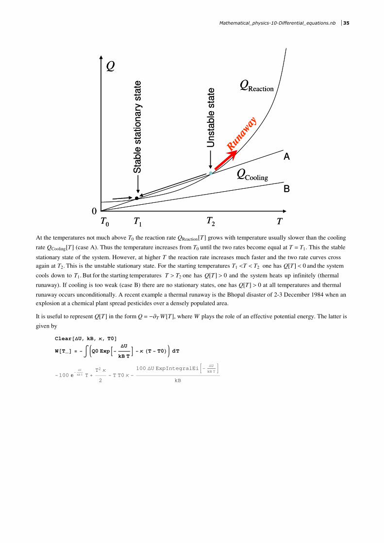
environment. The stability-instability of Semenov's temperature equation is explained in the plot below.


TT0

ReactionQ

CoolingQ

B

A

•

•

Sta

ble

sta

tion

ary

sta

te

T1T2

0

Q

Unsta

ble

sta

te

Run

away

TT0

ReactionQ

CoolingQ

B

A

•

•

Sta

ble

sta

tion

ary

sta

te

T1T2

0

Q

Unsta

ble

sta

te

Run

away

At the temperatures not much above T0 the reaction rate QReaction@TD grows with temperature usually slower than the cooling

rate QCooling@TD (case A). Thus the temperature increases from T0 until the two rates become equal at T = T1. This the stable

stationary state of the system. However, at higher T the reaction rate increases much faster and the two rate curves cross

again at T2. This is the unstable stationary state. For the starting temperatures T1 T T2 one has Q@TD 0 and the system

cools down to T1. But for the starting temperatures T > T2 one has Q@TD > 0 and the system heats up infinitely (thermal

runaway). If cooling is too weak (case B) there are no stationary states, one has Q@TD > 0 at all temperatures and thermal

runaway occurs unconditionally. A recent example a thermal runaway is the Bhopal disaster of 2-3 December 1984 when an

explosion at a chemical plant spread pesticides over a densely populated area.

It is useful to represent Q@TD in the form Q = -∑T W @TD, where W plays the role of an effective potential energy. The latter is

given by

Clear@∆U, kB, κ, T0DW@T_D = −‡ Q0 ExpB− ∆U

kB TF − κ HT − T0L T

−100 �−

∆U

kB T T +T2 κ

2− T T0 κ −

100 ∆U ExpIntegralEiB− ∆U

kB TF

kB


∆U = 10; kB = 1; Q0 = 100; T0 = 1; κ = 2;H∗ Parameters have to be carefully chosen ∗LPlot@W@TD, 8T, 0, 5<D

1 2 3 4 5

-3

-2

-1

1

Semenov's equation for the temperature in the form

C�T

�t� −

�W

�T

is mathematically equivalent to that for an overdamped particle sliding down the potential energy W @TD.

Semenov's model does not take into account that the amount of the explosive decreased as a result of burning. Thus this

model yields an infinite increase of the temperature in the thermal runaway. A more realistic model uses two first-order

differential equations, one for the temperature T and one for the mass of the fuel (explosive) m

C�T

�t� −Em

�m

�t− κ HT − T0L

�m

�t= −Γ@TD m, Γ@TD = Γ0 ExpB− ∆U

kB TF.

Here Em is the energy released by burning of one unit mass of the fuel and G@TD is the burning rate of the fuel. Substituting

the second equation into the first equation, one obtains Semenov's equation with QReaction@TD = Em m G@TD. To recover

Semenov's theory, one has to fix m to its initial value, to make the equation closed. Below is the numerical solution

∆U = 3000; T0 = 300; Em = 3000; c = 1;

Γ0 = 20; kB = 1; m0 = 1; H∗ κ=0.189; ∗LΓ@T_D := Γ0 ExpB− ∆U

T kBF

tMax = 500;

Eqm = m'@tD � −Γ@T@tDD m@tD;EqT@κ_D = c T'@tD + Em m'@tD � −κ HT@tD − T0L;sol@κ_D := NDSolve@8Eqm, EqT@κD, m@0D � m0, T@0D � T0<, 8m, T<, 8t, 0, tMax<D;mt@κ_, t_D := m@tD ê. First@sol@κDDTt@κ_, t_D := T@tD ê. First@sol@κDD

For k = 0.188 there is a thermal runaway with fast and complete burning but for k = 0.189 there is only a slow burning. Such

dependence of the solution of a differential equation on a parameter is called bifurcation.


Plot@[email protected], ttD, [email protected], ttD<, 8tt, 0, tMax<, PlotRange → 80, 1<,PlotStyle → 88Thick, Red<, 8Thick, Blue<<D H∗ cannot use t ∗L

0 100 200 300 400 500

0.2

0.4

0.6

0.8

1.0

In the case of thermal runaway temperature peaks and then returns to normal after all fuel is burned.

Plot@[email protected], ttD, [email protected], ttD<, 8tt, 0, 0.4 tMax<, PlotRange → All,

PlotStyle → 88Thick, Red<, 8Thick, Blue<<D H∗ cannot use t ∗L

50 100 150 200

1000

1500

2000


mathematical physics-10-differential equations mathematica, one writes systems of equations in a...

Documents