mathematical sketching, a novel, pen-based,cs.brown.edu/people/jjl/pubs/laviola_dissertation.pdf ·...
TRANSCRIPT

Abstract of “Mathematical Sketching: A New Approach to Creating and Exploring Dy-
namic Illustrations” by Joseph J. LaViola Jr., Ph.D., Brown University, May 2005.
Diagrams and illustrations are frequently used to help explain mathematical concepts. Stu-
dents often create them with pencil and paper as an intuitive aid in visualizing relationships
among variables, constants, and functions, and use them as a guide in writing the appro-
priate mathematics to solve the problem. However, such static diagrams generally assist
only in the initial formulation of the required mathematics, not in “debugging” or problem
analysis. This can be a severe limitation, even for simple problems with a natural mapping
to the temporal dimension or problems with complex spatial relationships.
To overcome these limitations we present mathematical sketching, a novel, pen-based,
gestural interaction paradigm for mathematics problem solving. Mathematical sketching de-
rives from the familiar pencil-and-paper process of drawing supporting diagrams to facilitate
the formulation of mathematical expressions; however, with mathematical sketching, users
can also leverage their physical intuition by watching their hand-drawn diagrams animate
in response to continuous or discrete parameter changes in their written formulas. Diagram
animation is driven by implicit associations that are inferred, either automatically or with
gestural guidance, from mathematical expressions, diagram labels and drawing elements.
We describe the critical components of mathematical sketching as developed in the con-
text of a prototype application called MathPad2. We discuss the important issues of the
mathematical sketching paradigm such as the development of a fluid gestural user interface,
recognition of mathematical expressions, support for computational tools such as graph-
ing, solving equations, and evaluating expressions, and the preparation and translation of
mathematical sketches into animated illustrations. Additionally, we present an evaluation of
MathPad2 and show that it is a powerful, easy-to-use tool for creating dynamic illustrations
and mathematical visualizations.

Mathematical Sketching: A New Approach to Creating and Exploring Dynamic
Illustrations
by
Joseph J. LaViola Jr.
B. S., Computer Science, Florida Atlantic University, 1996
Sc. M., Computer Science, Brown University, 2000
Sc. M., Applied Mathematics, Brown University, 2001
A dissertation submitted in partial fulfillment of the
requirements for the Degree of Doctor of Philosophy
in the Department of Computer Science at Brown University
Providence, Rhode Island
May 2005

c© Copyright 2004-2005 by Joseph J. LaViola Jr.

This dissertation by Joseph J. LaViola Jr. is accepted in its present form by
the Department of Computer Science as satisfying the dissertation requirement
for the degree of Doctor of Philosophy.
DateAndries van Dam, Director
Recommended to the Graduate Council
DateJohn F. Hughes, Reader
DateDavid H. Laidlaw, Reader
Approved by the Graduate Council
DateKaren Newman
Dean of the Graduate School
iii

Abstract
Diagrams and illustrations are frequently used to help explain mathematical concepts. Stu-
dents often create them with pencil and paper as an intuitive aid in visualizing relationships
among variables, constants, and functions, and use them as a guide in writing the appro-
priate mathematics to solve the problem. However, such static diagrams generally assist
only in the initial formulation of the required mathematics, not in “debugging” or problem
analysis. This can be a severe limitation, even for simple problems with a natural mapping
to the temporal dimension or problems with complex spatial relationships.
To overcome these limitations we present mathematical sketching, a novel, pen-based,
gestural interaction paradigm for mathematics problem solving. Mathematical sketching de-
rives from the familiar pencil-and-paper process of drawing supporting diagrams to facilitate
the formulation of mathematical expressions; however, with mathematical sketching, users
can also leverage their physical intuition by watching their hand-drawn diagrams animate
in response to continuous or discrete parameter changes in their written formulas. Diagram
animation is driven by implicit associations that are inferred, either automatically or with
gestural guidance, from mathematical expressions, diagram labels and drawing elements.
We describe the critical components of mathematical sketching as developed in the con-
text of a prototype application called MathPad2. We discuss the important issues of the
mathematical sketching paradigm such as the development of a fluid gestural user interface,
recognition of mathematical expressions, support for computational tools such as graph-
ing, solving equations, and evaluating expressions, and the preparation and translation of
mathematical sketches into animated illustrations. Additionally, we present an evaluation of
MathPad2 and show that it is a powerful, easy-to-use tool for creating dynamic illustrations
and mathematical visualizations.
iv

Vita
Joseph J. LaViola Jr. was born on February 12, 1974 in Warwick, RI.
Education
• Ph.D. in Computer Science, Brown University, Providence, RI, May 2005.
• Sc.M. in Applied Mathematics, Brown University, Providence, RI, May 2001.
• Sc.M. in Computer Science, Brown University, Providence, RI, May 2000.
• B.S. in Computer Science, Florida Atlantic University, Boca Raton, FL, May 1996.
Honors
• The van Dam Fellowship, Brown University, 2000-2002, 2004.
• IBM Cooperative Fellowship, IBM, 1998.
• Aaron Finerman Award, Florida Atlantic University, 1996.
• Faculty Award for Outstanding Undergraduate Achievement, Florida Atlantic Univer-
sity, 1996.
• Microsoft Senior Achievement Award, Microsoft, 1995.
v

Invited Talks
• Mathematical Sketching: A New Approach for Creating and Exploring Dynamic Illus-
trations, Microsoft Research, Seattle, WA, February 2005.
• Mathematical Sketching: A New Approach for Creating and Exploring Dynamic Illus-
trations, IBM T.J. Watson Research Center, Hawthorne, NY, December 2004.
Book
• Bowman, Doug, Ernst Kruijff, Joseph LaViola, and Ivan Poupyrev. 3D User Inter-
faces: Theory and Practice, Addison-Wesley, Boston, July 2004.
Master’s Thesis
• LaViola, Joseph. Whole-Hand and Speech Input in Virtual Environments, Master’s
Thesis, Brown University, Department of Computer Science, December 1999.
Refereed Journals Articles and Periodicals
• LaViola, Joseph. and Robert Zeleznik. MathPad2 : A System for the Creation and
Exploration of Mathematical Sketches”, ACM Transactions on Graphics (Proceedings
of SIGGRAPH 2004), 23(3):432-440, ACM Press, August 2004.
• Bowman, Doug, Ernst Kruijff, Joseph LaViola, and Ivan Poupyrev. An Introduction
to 3-D User Interface Design, PRESENCE: Teleoperators and Virtual Environments,
10(1):96-108, MIT Press, February 2001.
• van Dam, Andries, Andrew Forsberg, David Laidlaw, Joseph LaViola, and Rose-
mary Simpson. Immersive VR for Scientific Visualization: A Progress Report, IEEE
Computer Graphics and Applications, 20(6):26-52, IEEE Press, November/December
2000.
vi

• LaViola, Joseph. A Discussion of Cybersickness in Virtual Environments, SIGCHI
Bulletin, 32(1):47-56, ACM Press, January 2000.
• Forsberg, Andrew, Joseph LaViola, Lee Markosian, and Robert Zeleznik. Seamless
Interaction in Virtual Reality, IEEE Computer Graphics and Applications, 17(6):6-9,
IEEE Press, November/December 1997.
Reviewed Conference and Workshop Papers
• Julier, Simon and Joseph LaViola. An Empirical Study into the Robustness of Split
Covariance Addition (SCA) for Human Motion Tracking, Proceedings of the 2004
American Control Conference, IEEE Press, 2190-2195, June 2004.
• LaViola, Joseph. A Comparison of Unscented and Extended Kalman Filtering for
Estimating Quaternion Motion, Proceedings of the 2003 American Control Conference,
IEEE Press, 2435-2440, June 2003.
• LaViola, Joseph. A Testbed for Studying and Choosing Predictive Tracking Algo-
rithms in Virtual Environments, Proceedings of Immersive Projection Technology and
Virtual Environments 2003, ACM Press, 189-198, May 2003.
• LaViola, Joseph. Double Exponential Smoothing: An Alternative to Kalman Filter-
Based Predictive Tracking, Proceedings of Immersive Projection Technology and Vir-
tual Environments 2003, ACM Press, 199-206, May 2003.
• LaViola, Joseph. An Experiment Comparing Double Exponential Smoothing and
Kalman Filter-Based Predictive Tracking Algorithms, Proceedings of Virtual Reality
2003, IEEE Press, 283-284, March 2003.
• Zeleznik, Robert, Joseph LaViola, Daniel Acevedo, and Daniel Keefe. Pop Through
Buttons for Virtual Environment Navigation and Interaction, Proceedings of Virtual
Reality 2002, 127-134, IEEE Press, March 2002.
• LaViola, Joseph, Daniel Acevedo, Daniel Keefe, and Robert Zeleznik. Hands-Free
Multi-Scale Navigation in Virtual Environments, Proceedings of the 2001 Symposium
vii

on Interactive 3D Graphics, 9-15, ACM Press, March 2001.
• Keefe, Daniel, Daniel Acevedo, Tomer Moscovich, David Laidlaw, and Joseph LaViola.
CavePainting: A Fully Immersive 3D Artistic Medium and Interactive Experience,
Proceedings of the 2001 Symposium on Interactive 3D Graphics, 85-93, ACM Press,
March 2001.
• LaViola, Joseph. MSVT: A Virtual Reality-Based Multimodal Scientific Visualiza-
tion Tool, Proceedings of the Third IASTED International Conference on Computer
Graphics and Imaging, 1-7, Acta Press, November 2000.
• LaViola, Joseph and Robert Zeleznik. Flex and Pinch: A Case Study of Whole Hand
Input Design for Virtual Environment Interaction, Proceedings of the Second IASTED
International Conference on Computer Graphics and Imaging, 221-225, Acta Press,
October 1999.
• LaViola, Joseph. A Multimodal Interface Framework For Using Hand Gestures and
Speech in Virtual Environment Applications. Lecture Notes in Artificial Intelligence
#1739, Gesture-Based Communication in Human-Computer Interaction, 303-314,
Springer-Verlag, March 1999.
• LaViola, Joseph, Loring Holden, Andrew Forsberg, Dom Bhuphaibool, and Robert
Zeleznik. Collaborative Conceptual Modeling Using the SKETCH Framework, Pro-
ceedings of the First IASTED International Conference on Computer Graphics and
Imaging, 154-158, Acta Press, June 1998.
• Forsberg, Andrew, Joseph LaViola, and Robert Zeleznik. ErgoDesk: A Framework
for Two and Three Dimensional Interaction at the ActiveDesk, Proceedings of the
Second International Immersive Projection Technology Workshop, Ames, Iowa, May
11-12, 1998.
• LaViola, Joseph, Robert Barton, Ammo Goettsch, and Robert Cross. A Real-Time
Distributed Virtual Environment for Collaborative Engineering, Proceedings of Com-
puter Applications in Production and Engineering(CAPE), 712-726, November 1997.
viii

Courses and Tutorials
• Bowman, Doug, Joseph LaViola, Mark Mine, and Ivan Poupyrev. Advanced Topics
in 3D User Interface Design, Course #44, presented at ACM SIGGRAPH 2001, Los
Angeles, CA, August 2001.
• Bowman, Doug. Ernst Kruijff, Joseph LaViola, Mark Mine, and Ivan Poupyrev. 3D
User Interface Design: Fundamental Techniques, Theory, and Practice, Course #36,
presented at ACM SIGGRAPH 2000, New Orleans, LA, July 2000.
• Bowman, Doug, Ernst Kruijff, Joseph LaViola, and Ivan Poupyrev. The Art and
Science of 3D Interaction, full-day tutorial presented at IEEE Virtual Reality 2000,
New Brunswick, NJ, March 2000.
• Bowman, Doug, Ernst Kruijff, Joseph LaViola, and Ivan Poupyrev. The Art and
Science of 3D Interaction, full-day tutorial presented at the ACM Symposium on
Virtual Reality Software and Technology, London, December 1999.
• Bowman, Doug, Ernst Kruijff, Joseph LaViola, and Ivan Poupyrev. The Art and
Science of 3D Interaction, full-day tutorial presented at IEEE Virtual Reality ’99,
Houston, TX, March, 1999.
Miscellaneous Publications
• Zeleznik, Robert, Timothy Miller, Loring Holden, and Joseph LaViola. Fluid Inking:
Using Punctuation to Allow Modeless Combination of Marking and Gesturing, Techni-
cal Report CS-04-11, Brown University, Department of Computer Science, Providence,
RI, July 2004.
• LaViola, Joseph, Daniel Keefe, Robert Zeleznik, and Daniel Acevedo. Case Studies in
Building Custom Input Devices for Virtual Environment Interaction, Proceedings of
the IEEE VR 2004 Workshop on Beyond Wand and Glove-Based Interaction, 67-71,
March 2004.
ix
• Reiter, Jonathan, R.M. Kirby, and Joseph LaViola. Immersive Hierarchical Visual-
ization and Steering for Spectral/hp Element Methods, Technical Report CS-01-03,
Brown University, Department of Computer Science, Providence, RI, May 2001.
• Pickering, Jeffrey, Dom Bhuphaibool, Joseph LaViola, and Nancy Pollard. The
Coach’s Playbook, Technical Report CS-99-08, Brown University, Department of
Computer Science, Providence, RI, May 1999.
• Forsberg, Andrew, Joseph LaViola, and Robert Zeleznik. Incorporating Speech Input
into Gesture-Based Graphics Applications at The Brown University Graphics Lab,
CHI’99 Workshop on Designing the User Interface for Pen and Speech Multimedia
Applications, May 1999.
• LaViola, Joseph. Analysis of Mouse Movement Time Based on Varying Control to
Display Ratios Using Fitts’ Law, Technical Report CS-97-17, Brown University, De-
partment of Computer Science, Providence, RI, October 1997.
x

Acknowledgments
It has been a long and difficult road to get to this point in my career, but it has been a road
of great learning and discovery. It has also been a road where great life-long friendships
have been forged. I could have never completed my dissertation without the help of many
people. First, I must thank Andy van Dam, my advisor not only in research but in life,
for taking a chance on me and standing up for me during the tough times. I will always
be grateful for your guidance and friendship. I also want to thank John Hughes and David
Laidlaw, my thesis committee members, for their support and guidance over the years and
for their their help in directing the course of my research.
I want to thank Bob Zeleznik, who is like a brother to me, for his guidance and advice and
for our many collaborations over the years, not just in research but in winning intramural
sports championships as well.
I want to thank the members of the Brown Graphics Group, past and present espe-
cially Daniel Keefe, Daniel Acevedo, Andy Forsberg, Loring Holden, Tim Miller, Steven
Dollins, Tim Rowley, Lee Markosian, Christine Waggoner, Jonathan Reiter, Mike Kirby,
Jeff Pickering, Dan Gould, Jennifer Stewart, and Dom Bhuphailbool for their assistance
and collaboration on various projects I have had the pleasure of working on over the years.
A special thanks goes to Kazutoshi Yamazaki for working on the mathematical expres-
sion parsing system described in Chapter 6 as part of his master’s work. Without Kazu’s
hard work, I would not have been able to as make as much progress as I did with mathe-
matical sketching. Thanks to Tim Miller for providing the implementation summarized in
Algorithm 5.3 and to those who volunteered to participate in the user evaluation. Thanks
xi

to Trina Avery for her help in preparing this manuscript. I also want to thank my spon-
sors, Microsoft, NSF, and the Joint Advanced Distributed Co-Laboratory, for their financial
support.
Pursuing a PhD can be an isolating experience and I could not have succeeded without
great friendships and social outlets. Thus, I want to thank two of my best friends, Don
Carney and David Gondek, for their friendship and support over the years. Thanks for the
OMWs and Brouhahas. I also want to thank all of the members of the Brown Computer
Science Intramural football and softball teams for being great teammates.
Last but certainly not least, I want to thank family especially my mom, dad, and Jamie,
for supporting me in everything I have ever wanted to do. You are the most important people
in my life. Finally, to everyone who asks me, “Are you finished yet?”, I can now answer,
“YES!”
xii

Contents
List of Tables xviii
List of Figures xix
1 Introduction 1
1.1 The Problem . . . . . . . . . . . . . . . . . . . . . . . . . . . . . . . . . . . 1
1.2 Mathematical Sketching . . . . . . . . . . . . . . . . . . . . . . . . . . . . . 2
1.3 Example Scenarios . . . . . . . . . . . . . . . . . . . . . . . . . . . . . . . . 4
1.3.1 Two Cars — Constant Velocity vs. Constant Acceleration . . . . . . 4
1.3.2 2D Projectile Motion . . . . . . . . . . . . . . . . . . . . . . . . . . . 5
1.3.3 2D Projectile Motion with Air Drag . . . . . . . . . . . . . . . . . . 6
1.4 Research Contributions . . . . . . . . . . . . . . . . . . . . . . . . . . . . . 8
1.5 Reader’s Guide . . . . . . . . . . . . . . . . . . . . . . . . . . . . . . . . . . 8
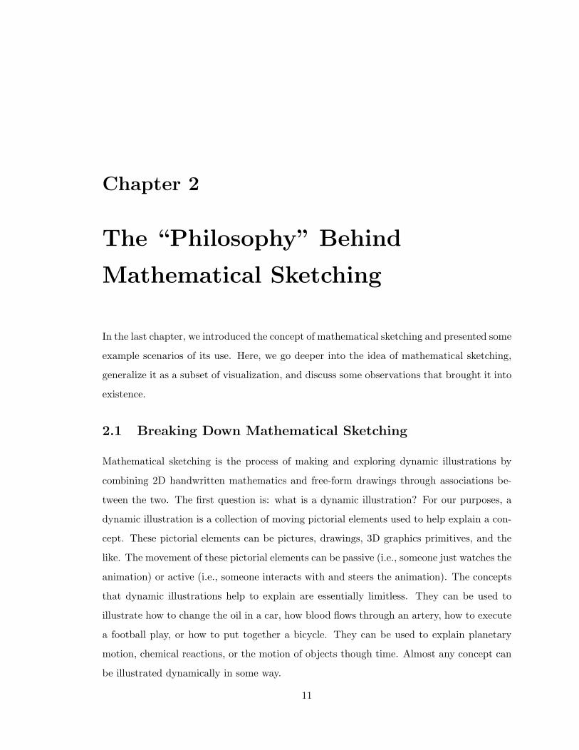
2 The “Philosophy” Behind Mathematical Sketching 11
2.1 Breaking Down Mathematical Sketching . . . . . . . . . . . . . . . . . . . . 11
2.2 Generalizing Mathematical Sketching as a Paradigm . . . . . . . . . . . . . 14
2.3 Observations on Mathematical Sketching . . . . . . . . . . . . . . . . . . . . 16
3 Related Work 18
3.1 WIMP-based and Programmatic Dynamic Illustration . . . . . . . . . . . . 18
3.2 Gestural User Interfaces . . . . . . . . . . . . . . . . . . . . . . . . . . . . . 21
3.3 Pen-Based Dynamic Illustration . . . . . . . . . . . . . . . . . . . . . . . . . 22
3.4 Computational and Symbolic Math Engines . . . . . . . . . . . . . . . . . . 23
xiii

3.5 Mathematical Expression Recognition and Applications . . . . . . . . . . . 23
4 A User Interface for Mathematical Sketching 25
4.1 Design Goals and Strategy . . . . . . . . . . . . . . . . . . . . . . . . . . . . 25
4.2 Writing Mathematical Expressions . . . . . . . . . . . . . . . . . . . . . . . 28
4.2.1 Inking . . . . . . . . . . . . . . . . . . . . . . . . . . . . . . . . . . . 29
4.2.2 Recognizing Mathematical Expressions . . . . . . . . . . . . . . . . . 31
4.2.3 Feedback . . . . . . . . . . . . . . . . . . . . . . . . . . . . . . . . . 32
4.2.4 Correcting Recognition Errors . . . . . . . . . . . . . . . . . . . . . . 35
4.3 Making Drawings . . . . . . . . . . . . . . . . . . . . . . . . . . . . . . . . . 38
4.3.1 Nailing Diagram Components . . . . . . . . . . . . . . . . . . . . . . 38
4.3.2 Grouping Diagram Components . . . . . . . . . . . . . . . . . . . . 39
4.4 Associations . . . . . . . . . . . . . . . . . . . . . . . . . . . . . . . . . . . . 40
4.4.1 Implicit Associations . . . . . . . . . . . . . . . . . . . . . . . . . . . 40
4.4.2 Explicit Associations . . . . . . . . . . . . . . . . . . . . . . . . . . . 43
4.5 Supporting Mathematical Toolset . . . . . . . . . . . . . . . . . . . . . . . . 46
4.5.1 Graphing Equations . . . . . . . . . . . . . . . . . . . . . . . . . . . 46
4.5.2 Solving Equations . . . . . . . . . . . . . . . . . . . . . . . . . . . . 48
4.5.3 Evaluating Expressions . . . . . . . . . . . . . . . . . . . . . . . . . 49
4.6 Issues Arising with Digital Ink . . . . . . . . . . . . . . . . . . . . . . . . . 52
5 Mathematical Symbol Recognition 57
5.1 The Problem . . . . . . . . . . . . . . . . . . . . . . . . . . . . . . . . . . . 57
5.2 Previous Work in Mathematical Symbol Recognition . . . . . . . . . . . . . 58
5.3 Writer Dependence and The Training Application . . . . . . . . . . . . . . . 60
5.3.1 User Training . . . . . . . . . . . . . . . . . . . . . . . . . . . . . . . 61
5.4 Previous Symbol Recognizers in Mathematical Sketching . . . . . . . . . . . 63
5.4.1 Using Microsoft’s Handwriting Recognizer . . . . . . . . . . . . . . . 63
5.4.2 Using Dominant Points and Linear Classification . . . . . . . . . . . 64
5.5 The Pairwise AdaBoost/Microsoft Handwriting Recognizer Algorithm . . . 65
5.5.1 Preprocessing . . . . . . . . . . . . . . . . . . . . . . . . . . . . . . . 66
xiv

5.5.2 Symbol Segmentation . . . . . . . . . . . . . . . . . . . . . . . . . . 67
5.5.3 Statistical and Geometric Features . . . . . . . . . . . . . . . . . . . 69
5.5.4 AdaBoost Learning . . . . . . . . . . . . . . . . . . . . . . . . . . . . 77
5.5.5 The Recognition Algorithm . . . . . . . . . . . . . . . . . . . . . . . 78
6 Mathematical Expression Parsing 83
6.1 The Problem . . . . . . . . . . . . . . . . . . . . . . . . . . . . . . . . . . . 83
6.2 Related Work in Mathematical Expression Parsing . . . . . . . . . . . . . . 86
6.3 The Parsing Algorithm . . . . . . . . . . . . . . . . . . . . . . . . . . . . . . 89
6.3.1 Parsing and Writer Dependence . . . . . . . . . . . . . . . . . . . . . 90
6.3.2 Parsing Grammar and Algorithm Summary . . . . . . . . . . . . . . 91
6.3.3 Implicit Operators . . . . . . . . . . . . . . . . . . . . . . . . . . . . 95
6.3.4 Fractions and Square Roots . . . . . . . . . . . . . . . . . . . . . . . 96
6.3.5 Summations, Integrals, and Derivatives . . . . . . . . . . . . . . . . 97
6.3.6 Conditionals . . . . . . . . . . . . . . . . . . . . . . . . . . . . . . . 100
6.3.7 Reducing Parsing Decisions and Improving Symbol Recognition . . . 101
7 Mathematical Sketch Preparation 103
7.1 Mathematical Sketch Preparation Components . . . . . . . . . . . . . . . . 103
7.2 Association Inferencing . . . . . . . . . . . . . . . . . . . . . . . . . . . . . . 104
7.3 Drawing Dimension Analysis . . . . . . . . . . . . . . . . . . . . . . . . . . 106
7.4 Drawing Rectification . . . . . . . . . . . . . . . . . . . . . . . . . . . . . . 109
7.4.1 Angle Rectification . . . . . . . . . . . . . . . . . . . . . . . . . . . . 110
7.4.2 Location Rectification . . . . . . . . . . . . . . . . . . . . . . . . . . 112
7.4.3 Size Rectification . . . . . . . . . . . . . . . . . . . . . . . . . . . . . 116
7.5 Stretch Determination . . . . . . . . . . . . . . . . . . . . . . . . . . . . . . 119
8 Mathematical Sketch Translation and Animation 121
8.1 Translating Mathematical Sketches into Executable Code . . . . . . . . . . 121
8.1.1 Closed-Form Solutions . . . . . . . . . . . . . . . . . . . . . . . . . . 123
8.1.2 Open-Form Solutions . . . . . . . . . . . . . . . . . . . . . . . . . . . 126
xv

8.2 The Animation System . . . . . . . . . . . . . . . . . . . . . . . . . . . . . . 131
9 MathPad2 133
9.1 Functionality Summary . . . . . . . . . . . . . . . . . . . . . . . . . . . . . 133
9.2 Software Architecture . . . . . . . . . . . . . . . . . . . . . . . . . . . . . . 135
10 Recognizer Accuracy and MathPad2 Usability Experiments 138
10.1 User Evaluation Goals . . . . . . . . . . . . . . . . . . . . . . . . . . . . . . 138
10.2 Mathematical Symbol and Expression Recognition Study . . . . . . . . . . 139
10.2.1 Experimental Design and Tasks . . . . . . . . . . . . . . . . . . . . . 139
10.2.2 Participants . . . . . . . . . . . . . . . . . . . . . . . . . . . . . . . . 142
10.2.3 Evaluation Measures . . . . . . . . . . . . . . . . . . . . . . . . . . . 142
10.2.4 Results and Discussion . . . . . . . . . . . . . . . . . . . . . . . . . . 144
10.3 MathPad2 Usability Study . . . . . . . . . . . . . . . . . . . . . . . . . . . 149
10.3.1 Experimental Design and Tasks . . . . . . . . . . . . . . . . . . . . . 149
10.3.2 Participants . . . . . . . . . . . . . . . . . . . . . . . . . . . . . . . . 153
10.3.3 Evaluation Measures . . . . . . . . . . . . . . . . . . . . . . . . . . . 153
10.3.4 Results and Discussion . . . . . . . . . . . . . . . . . . . . . . . . . . 154
11 Discussion and Future Work 161
11.1 Discussion . . . . . . . . . . . . . . . . . . . . . . . . . . . . . . . . . . . . . 161
11.1.1 Further Observations . . . . . . . . . . . . . . . . . . . . . . . . . . . 161
11.1.2 Current Limitations of Mathematical Sketching . . . . . . . . . . . . 164
11.2 Future Work . . . . . . . . . . . . . . . . . . . . . . . . . . . . . . . . . . . 165
11.2.1 Plausibility Concerns . . . . . . . . . . . . . . . . . . . . . . . . . . . 166
11.2.2 Improving Mathematical Expression Recognition . . . . . . . . . . . 166
11.2.3 Expanding Mathematical Sketching . . . . . . . . . . . . . . . . . . 171
11.2.4 Extensibility . . . . . . . . . . . . . . . . . . . . . . . . . . . . . . . 183
11.2.5 Other Mathematical Sketching Ideas . . . . . . . . . . . . . . . . . . 186
11.3 Summing Up Mathematical Sketching . . . . . . . . . . . . . . . . . . . . . 188
12 Conclusion 189
xvi

A MathPad2 Prototype History 191
A.1 Prototype One . . . . . . . . . . . . . . . . . . . . . . . . . . . . . . . . . . 191
A.2 Prototype Two . . . . . . . . . . . . . . . . . . . . . . . . . . . . . . . . . . 193
A.3 Prototype Three . . . . . . . . . . . . . . . . . . . . . . . . . . . . . . . . . 195
B Subject Questionnaires 198
B.1 Pre-Questionnaire . . . . . . . . . . . . . . . . . . . . . . . . . . . . . . . . 198
B.2 Post-Questionnaire . . . . . . . . . . . . . . . . . . . . . . . . . . . . . . . . 199
C Mathematical Expressions Used in Recognition Experiments 202
Bibliography 204
? Parts of this dissertation have been previously published in [LaViola and Zeleznik 2004],
co-written with Robert C. Zeleznik.
xvii

List of Tables
6.1 Some 2D mathematical expressions and their 1D representations. . . . . . . 90
10.1 Accuracy of recognizers A and B with symbol data from the symbol and
mathematical expression tests. . . . . . . . . . . . . . . . . . . . . . . . . . 145
10.2 Subjects’ average ratings of their overall reaction to MathPad2 on a scale
from 1 to 7. . . . . . . . . . . . . . . . . . . . . . . . . . . . . . . . . . . . . 156
10.3 Subjects’ average ratings of ease of use for different components of the MathPad2
user interface (scale: 1=easy, 7=hard). . . . . . . . . . . . . . . . . . . . . 157
10.4 Subjects’ average ratings of the perceived usefulness of MathPad2 in their
work (scale: 1=unlikely, 7=likely). . . . . . . . . . . . . . . . . . . . . . . . 159
xviii

List of Figures
1.1 Diagram of the initial formulation for analyzing the differences between
constant velocity and constant acceleration of two vehicles (adapted from
[Ford 1992]). . . . . . . . . . . . . . . . . . . . . . . . . . . . . . . . . . . . 2
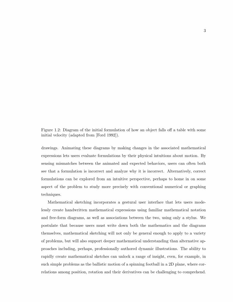
1.2 Diagram of the initial formulation of how an object falls off a table with some
initial velocity (adapted from [Ford 1992]). . . . . . . . . . . . . . . . . . . . 3
1.3 A mathematical sketch of two cars moving down a road, one with constant
velocity and one with constant acceleration. The student writes down the
mathematics, draws a road and two cars, and associates the mathematics
to the drawing using labels. Running the sketch animates the two cars,
illuminating how a car moving with constant acceleration will overtake the
car with constant velocity. The sketch also shows a graph of the two equations
of motion. . . . . . . . . . . . . . . . . . . . . . . . . . . . . . . . . . . . . . 5
1.4 An ill-specified mathematical sketch determining if a baseball will fly over a
fence for a home run. After running the sketch, the user will clearly see an
error since the ball will fly upward in a parabolic fashion. . . . . . . . . . . 6
1.5 A mathematical sketch illustrating how air drag affects a ball’s 2D motion.
The sketch uses a simple Euler integration method to determine the ball’s
position through time. Associations between mathematics and drawings are
color-coded. . . . . . . . . . . . . . . . . . . . . . . . . . . . . . . . . . . . . 7
xix

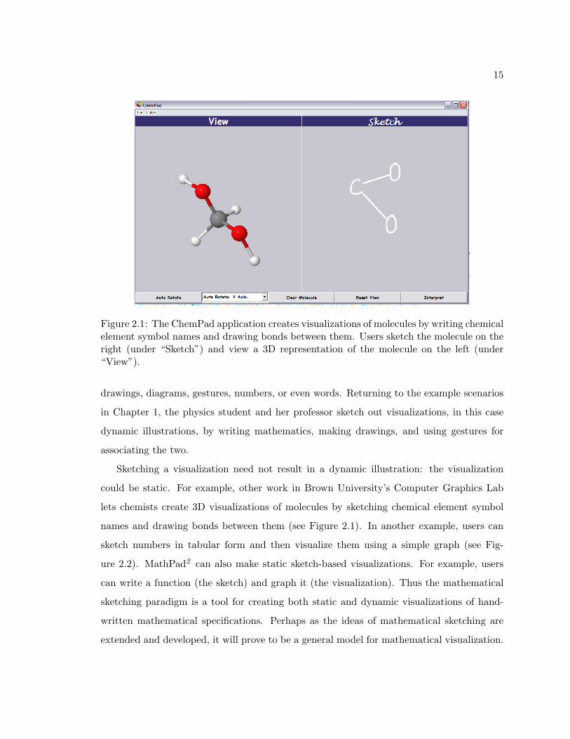
2.1 The ChemPad application creates visualizations of molecules by writing chem-
ical element symbol names and drawing bonds between them. Users sketch
the molecule on the right (under “Sketch”) and view a 3D representation of
the molecule on the left (under “View”). . . . . . . . . . . . . . . . . . . . . 15
2.2 A sketch-based visualization in which numbers in tabular form are visualized
with a graph. . . . . . . . . . . . . . . . . . . . . . . . . . . . . . . . . . . . 16
3.1 A dynamic illustration of an air track created with Interactive PhysicsTM. A
user creates the track using the primitives shown on the left of the application
window. Given these primitives, the underyling physics engine can animate
the blocks on the track appropriately. . . . . . . . . . . . . . . . . . . . . . 19
3.2 A dynamic illustration of 2D planetary motion created with The Geometer’s
SketchpadTM. The planets, moon, and sun are created with the circle tool
and the planets and moon are animated by specifying rotation points. . . . 20
3.3 Dynamic illustration of a ball thrown off a catapult into a pyramid of blocks.
The user has sketched the illustrations and the system recognizes the draw-
ings as geometric primitives. This version of the ASSIST system was devel-
oped as a power toy for Microsoft Tablet PCs. . . . . . . . . . . . . . . . . 22
4.1 A mathematical sketch exploring damped harmonic oscillation shows a draw-
ing of a spring and mass and the necessary equations for animating the draw-
ing. The label inside the mass associates the mathematics with the drawing. 26
4.2 Mathematical sketching gestures. Gesture strokes in the first column are
shown here in red. In the second column, cyan-highlighted strokes provide as-
sociation feedback (the highlighting color changes each time a new association
is made), and magenta strokes show nail and angle association/rectification
feedback. . . . . . . . . . . . . . . . . . . . . . . . . . . . . . . . . . . . . . 27
4.3 Scribbling over ink strokes and making a tap (top) erases the ink underneath
the scribble gesture (bottom). . . . . . . . . . . . . . . . . . . . . . . . . . . 29
4.4 A scribble whose bounding box is larger than the stroke itself. . . . . . . . . 30
xx

4.5 Mathematical expressions are recognized by drawing a lasso around them
and making a tap inside the lasso (top). Recognized mathematics is shown
in a red bounding box (bottom). . . . . . . . . . . . . . . . . . . . . . . . . 32
4.6 A written mathematical expression (top) and a recognized one (bottom).Even
though the recognized expression is presented in the user’s own handwriting,
recognition errors, such as a vertical line instead of a left parenthesis, are
easily discerned. . . . . . . . . . . . . . . . . . . . . . . . . . . . . . . . . . 33
4.7 What happens when the canonical symbol and recognized symbol have sig-
nificantly different aspect ratios. We special-case the square root symbol to
deal with this problem. . . . . . . . . . . . . . . . . . . . . . . . . . . . . . . 35
4.8 A menu of symbol alternatives. Here, the user’s “2” in front of the x2 was
recognized as an “h”. The user can correct the error by clicking on the first
menu item. . . . . . . . . . . . . . . . . . . . . . . . . . . . . . . . . . . . . 36
4.9 A menu of alternative expressions. The first menu item shows the recognizer’s
interpretation and the remaining menu items are the alternates. Here the
system recognized the ink as y = xt2: the correct expression, y = xt2 , is the
next-to-last menu item. . . . . . . . . . . . . . . . . . . . . . . . . . . . . . 37
4.10 A nail gesture connecting the top line with the vertical line (left). A correctly
recognized nail is indicated by a small red circle at the nail location (right). 39
4.11 A user draws a car, makes a lasso around it and taps on the lasso (top). The
green box surrounding the car shows that a composite drawing element has
been made (bottom). . . . . . . . . . . . . . . . . . . . . . . . . . . . . . . . 40
4.12 Lassoing 50 and tapping on the horizontal line between the tree and house
makes an implicit point association (top). The expression and drawing ele-
ment are highlighted in a pastel color to indicate the association was made
(bottom). . . . . . . . . . . . . . . . . . . . . . . . . . . . . . . . . . . . . . 41
xxi

4.13 The user writes an “a” underneath the pendulum, makes an angle arc, then
taps on the pendulum to make an implicit angle association (top); the green
dot shows the point of rotation and the magenta arrow shows which drawing
element will rotate (bottom). The angle changes to reflect a = 0.6. This is
called angle rectification and is discussed in Section 7.4.1. . . . . . . . . . . 42
4.14 A user draws a line through the mathematics; as the stylus hovers over the
ball, it turns cyan (top). With a tap, the mathematics is associated to the
ball and is highlighted along with the mathematics in a pastel color to confirm
that the association was made (bottom). . . . . . . . . . . . . . . . . . . . . 43
4.15 A graphing gesture (top) that graphs all three recognized functions and plots
them in a graph widget (bottom). . . . . . . . . . . . . . . . . . . . . . . . . 47
4.16 Two plots created using graph gestures. Expression bounding boxes are
colored to correspond to plot lines. . . . . . . . . . . . . . . . . . . . . . . . 48
4.17 A squiggle gesture through three equations (left), and the results of the si-
multaneous equation solve (right). . . . . . . . . . . . . . . . . . . . . . . . 49
4.18 The results of a ordinary differential equation solve on a second-order differ-
ential equation with initial condition. . . . . . . . . . . . . . . . . . . . . . . 50
4.19 A user evaluates an expression using an equal tap gesture (top), yielding a
simplification of the expression (bottom). . . . . . . . . . . . . . . . . . . . 51
4.20 A variety of expressions evaluated using the equal tap gesture. . . . . . . . 51
4.21 A simple stroke drawn with digital ink. . . . . . . . . . . . . . . . . . . . . 52
4.22 The top two plots show the beginning and ending points of the stroke in
Figure 4.21. The bottom two plots show the filtered versions of the beginning
and ending points of the original stroke. Note that the units for these plots
are in tenths of a millimeter. . . . . . . . . . . . . . . . . . . . . . . . . . . 53
5.1 The 1 in 12 and the l in log are indistinguishable. . . . . . . . . . . . . . . . 61
5.2 Training examples: writing “u”. . . . . . . . . . . . . . . . . . . . . . . . . 62
5.3 Training examples: writing “u” as small as possible. . . . . . . . . . . . . . 63
5.4 An ink stroke scaled up by a factor of 10. Stroke points are shown in magenta.
The end points are circular with their radii one half the pen width. . . . . . 68
xxii
6.1 How spatial relationships, sizes, and cases can make parsing difficult. . . . . 85
6.2 The context-free grammar used in part to parse mathematical expressions.
Note that, for brevity, <digit> and <letter> are written using regular ex-
pression notation. . . . . . . . . . . . . . . . . . . . . . . . . . . . . . . . . . 93
6.3 Mathematical expressions that are parsed correctly due to the aggressiveness
of the fraction rule. Even those symbols that are not completely within the
vertical boundary of the fraction are still included as part of the fraction’s
numerator and denominator. . . . . . . . . . . . . . . . . . . . . . . . . . . 97
6.4 Mathematical expressions that are parsed correctly due to the aggressiveness
of the square root rule. Even those symbols that are not completely contained
within the square root’s bounding box are still included in the square root
operation. . . . . . . . . . . . . . . . . . . . . . . . . . . . . . . . . . . . . . 97
6.5 Mathematical expressions that are parsed correctly due to the aggressiveness
of the summation rule. Even those symbols that are not completely contained
within the summation sign’s horizontal and vertical boundaries are included
as part of the summation. . . . . . . . . . . . . . . . . . . . . . . . . . . . . 98
6.6 Two different ways to write integration limits. . . . . . . . . . . . . . . . . . 99
6.7 A conditional expression. . . . . . . . . . . . . . . . . . . . . . . . . . . . . 100
7.1 The building and ground are labeled with constants and the stick figure is
labeled with the letter “p”. Individual drawing elements and the mathemat-
ical expressions are color-coded with a semi-transparent pastel color to show
the associations. . . . . . . . . . . . . . . . . . . . . . . . . . . . . . . . . . 105
7.2 Two methods for inferring coordinate dimensions: the mathematical sketch
on the left uses labeling of the ground line, while the one on the right uses
the calculated distance between h and s at time t = 0. . . . . . . . . . . . . 107
xxiii

7.3 The effects of labeling an angle: a user draws the pendulum on the left
and writes a = 0.5. When an angle label is made, the drawing is rectified
based on the initial value of a (in radians) and the pendulum on the right is
rotated to reflect a. The green dot shows the rotation point (computed using
Algorithm 4.4) and the magenta arrow shows which part of the drawing will
rotate during the dynamic illustration. . . . . . . . . . . . . . . . . . . . . . 110
7.4 Angle rectification breaks down when additional constraints are applied. The
top sketch shows a three-stroke triangle whose base is given a width of 200.
The bottom sketch shows an angle rectification made to the top angle that
breaks the triangle. The question here is whether the triangle should be
maintained. . . . . . . . . . . . . . . . . . . . . . . . . . . . . . . . . . . . 111
7.5 A mathematical sketch created to illustrate projectile motion with air drag. If
the ball labeled “p” is not positioned correctly with respect to the horizontal
line, it is difficult to verify whether the mathematics drives the ball over the
fence. . . . . . . . . . . . . . . . . . . . . . . . . . . . . . . . . . . . . . . . 113
7.6 The ball’s location is rectified before the illustration is run using the initial
conditions px(0) and py(0), the horizontal line, and the vertical line. . . . . 114
7.7 A mathematical sketch that showing a ball traveling in 1D, making an colli-
sion with a wall. If the ball (labeled “x”) is not the correct size in relation to
the x dimension and the mathematics, the illustration will not look correct
since the ball will not appear to hit and bounce off the wall. . . . . . . . . . 116
7.8 The ball’s size is rectified on the basis of its specified diameter and its re-
lationship with the horizontal line. Location rectification is done here as
well. . . . . . . . . . . . . . . . . . . . . . . . . . . . . . . . . . . . . . . . . 117
8.1 Different formats for the iteration construct. . . . . . . . . . . . . . . . . . . 124
8.2 A mathematical sketch: does the football go over the goalpost? . . . . . . . 126
8.3 The code generated from the mathematical specification in Figure 8.2. Note
that the variable t is an array of time values already placed into Matlab. . . 126
8.4 A mathematical sketch with an open-form solution. . . . . . . . . . . . . . . 127
8.5 Code generated from the mathematical specification in Figure 8.4. . . . . . 128
xxiv

8.6 A mathematical sketch with an open-form solution that has conditionals. . 129
8.7 Code generated from the mathematical specification in Figure 8.6. . . . . . 130
9.1 A diagram of MathPad2 ’s software architecture. . . . . . . . . . . . . . . . 136
10.1 The accuracy of mathematical symbol recognizers A and B for each subject
using the mathematical symbol test data. . . . . . . . . . . . . . . . . . . . 146
10.2 The accuracy of mathematical symbol recognizers A and B for each subject
using the mathematical expression test data. . . . . . . . . . . . . . . . . . 147
10.3 Parsing decision accuracy across subjects. . . . . . . . . . . . . . . . . . . . 148
10.4 The fourth task in the MathPad2 usability test. . . . . . . . . . . . . . . . . 151
10.5 Subjects create a damped harmonic oscillator in the fifth task. . . . . . . . 152
11.1 Our current conditional parsing algorithm fails to parse this expression cor-
rectly. By looking at pairs of symbols, we could construct a polyline (the red
line in between the two statements) to separate the two statements so they
can be parsed correctly. . . . . . . . . . . . . . . . . . . . . . . . . . . . . . 169
11.2 How a user might specify a user-defined function. The def and end keywords
signify the start and end of the function respectively. . . . . . . . . . . . . 177
11.3 An approximate solution to the heat equation on a rectangular metal plate. 186
11.4 Two snapshots of a dynamic illustration showing heat dissipating across a
metal plate given the mathematics in Figure 11.3. As the illustration runs,
the dots change color to show temperature changes. . . . . . . . . . . . . . 187
A.1 The first MathPad2 prototype. The drawing area shows the primitives that
the system could recognize (points, lines, and, graphs). Here, the user en-
ters variable names in the variable and constant declaration section and an
equation to graph in the program section. . . . . . . . . . . . . . . . . . . . 192
A.2 The second MathPad2 prototype. In this version, users could write mathe-
matical expressions and make drawings using a stylus. The text box at the
bottom of the application presents the results of recognized mathematical
expressions in a 1D notation. . . . . . . . . . . . . . . . . . . . . . . . . . . 194
xxv

A.3 The third MathPad2 prototype. In this version, users could specify rotations,
make composite objects, nail drawing elements to one another, and use a
gestural interface to invoke graphing and other operations. . . . . . . . . . 196
xxvi

Chapter 1
Introduction
Diagrams and illustrations are often used to help explain mathematical concepts. They
are commonplace in math and physics textbooks and provide a form of physical intuition
about abstract principles [Hecht 2000, Varberg and Purcell 1992, Young 1992]. Similarly,
students often draw pencil-and-paper diagrams for mathematics problems to help in visu-
alizing relationships among variables, constants, and functions, and use the drawing as a
guide to writing the appropriate mathematics for the problem.
1.1 The Problem
Unfortunately, static diagrams generally assist only in the initial formulation of a mathe-
matical problem, not in its “debugging”, analysis or complete visualization. Consider the
diagrams in Figures 1.1 and 1.2. In both cases, a student has a particular problem to solve
and draws a quick diagram with pencil and paper to get some intuition about how to set
it up. In Figure 1.1, the student wants to explore the difference between the motion of
two vehicles, one with constant velocity and one with constant acceleration. In Figure 1.2,
the student wants to understand how far an object pushed off a table will fall before it
hits the ground and how long it will take to do so. The student can use these diagrams to
help formulate the required mathematics to answer various possible questions about these
physical concepts.
However, once the solutions have been found, the diagrams become relatively useless.
The student cannot use them to check her answers or see if they make visual sense; she
1

2
Figure 1.1: Diagram of the initial formulation for analyzing the differences between constantvelocity and constant acceleration of two vehicles (adapted from [Ford 1992]).
cannot see any time-varying information associated with the diagram and cannot infer how
parameter changes affect her solutions. The student could use one of many educational
or mathematical software packages (see Chapter 3) to create a dynamic illustration of her
problem, but this would take her away from the pencil and paper she is comfortable with
and create a barrier between the mathematics she had written and the visualization created
on the computer. Because of these drawbacks, statically drawn diagrams have a lack of
expressive power that can be a severe limitation, even in simple problems with natural
mappings to the temporal dimension or in problems with complex spatial relationships.
1.2 Mathematical Sketching
With the advent of pen-based computers, it seems logical that the computer’s computational
power and the expressivity of pencil and paper could be combined to resolve many of the
drawbacks of static diagrams discussed above. Mathematical sketching addresses these
problems by combining the benefits of the familiar pencil-and-paper medium and the power
of a computer. More specifically, mathematical sketching is the process of making and
exploring dynamic illustrations by associating 2D handwritten mathematics with free-form
3
Figure 1.2: Diagram of the initial formulation of how an object falls off a table with someinitial velocity (adapted from [Ford 1992]).
drawings. Animating these diagrams by making changes in the associated mathematical
expressions lets users evaluate formulations by their physical intuitions about motion. By
sensing mismatches between the animated and expected behaviors, users can often both
see that a formulation is incorrect and analyze why it is incorrect. Alternatively, correct
formulations can be explored from an intuitive perspective, perhaps to home in on some
aspect of the problem to study more precisely with conventional numerical or graphing
techniques.
Mathematical sketching incorporates a gestural user interface that lets users mode-
lessly create handwritten mathematical expressions using familiar mathematical notation
and free-form diagrams, as well as associations between the two, using only a stylus. We
postulate that because users must write down both the mathematics and the diagrams
themselves, mathematical sketching will not only be general enough to apply to a variety
of problems, but will also support deeper mathematical understanding than alternative ap-
proaches including, perhaps, professionally authored dynamic illustrations. The ability to
rapidly create mathematical sketches can unlock a range of insight, even, for example, in
such simple problems as the ballistic motion of a spinning football in a 2D plane, where cor-
relations among position, rotation and their derivatives can be challenging to comprehend.
4
On the basis of these observations, the thesis of this dissertation is
Creating and exploring dynamic illustrations by combining handwritten 2D math-
ematics and free-form drawings with a modeless gestural user interface signifi-
cantly reduces the limitations of static diagrams used in mathematical problem
solving and visualization.
1.3 Example Scenarios
We present three user scenarios illustrating creating a mathematical sketch and using it in
solving a problem. The scenarios were chosen to illustrate both the use of mathematical
sketching to help solve a problem and the types of sketches that can be created. All these
scenarios have been created using MathPad2 , a prototype application developed to explore
the mathematical sketching paradigm. The first example concerns the differences between
a car moving with constant velocity and another moving with constant acceleration, the
second concerns 2D projectile motion, and the third concerns 2D projectile motion with air
drag.
1.3.1 Two Cars — Constant Velocity vs. Constant Acceleration
A physics student wants to understand how a police car p with constant acceleration ao
catches up to a speeding car m with a constant velocity vo. The student first draws a road
and the two cars and then writes down values for a0 and v0, as in Figure 1.1. However, in
the mathematical sketch, the student writes down the equations of motion and labels the
two cars to associate the mathematics to the drawings, as shown in Figure 1.3. The cars’
labels are used as a guide to infer which mathematical expressions are needed to animate
each car. The student can run the animation and visualize the dynamic behavior of the two
cars to gain insight into how car p moves over time relative to car m. This type of insight
would not be possible with a traditional pencil-and-paper medium. Note that the student
could also graph the equations of motion to see when car p will catch up with car m.

5
Figure 1.3: A mathematical sketch of two cars moving down a road, one with constantvelocity and one with constant acceleration. The student writes down the mathematics,draws a road and two cars, and associates the mathematics to the drawing using labels.Running the sketch animates the two cars, illuminating how a car moving with constantacceleration will overtake the car with constant velocity. The sketch also shows a graph ofthe two equations of motion.
1.3.2 2D Projectile Motion
Now the same physics student wants to determine if a baseball player can hit a ball over
a fence given an initial velocity and angle. She first draws the simple playing field shown
in Figure 1.4. Next she writes down the known quantities: the initial angle ao, initial
velocity vo, and the gravitational constant g. From her knowledge of projectile motion, she
then writes down the mathematics shown in Figure 1.4, labels the drawing, associates the
mathematics to the drawing by making a line gesture through the mathematical expressions
and tapping on the ball, and runs the animation. The animation shows the ball actually
moving upward against gravity, which is clearly wrong. She checks the equations and realizes
that Py(t) = voyt + 12gt2 has a sign error, so she scratches out the + and writes in a −. She
then runs the animation again: the ball takes on the correct motion and barely makes it

6
Figure 1.4: An ill-specified mathematical sketch determining if a baseball will fly over afence for a home run. After running the sketch, the user will clearly see an error since theball will fly upward in a parabolic fashion.
over the fence.
Next she wants to see how much farther the ball will go if vo is increased. She scratches
out this value, writes in a larger one, and runs the animation again. The ball does go farther,
but it also stops short of the ground, which leads her to the question, “When will the ball
hit the ground with these new parameters?” She takes equation Py(t), sets it equal to zero,
and solves it using a simple gesture. Finally, she takes the second value for t, changes the
time field, runs the animation and finds that this time value is correct: the ball hits the
ground with the new parameters. This type of dynamic interaction with the mathematical
sketch provides a “interactive notebook” that has the look and feel of a regular notebook
but has a powerful computational engine beneath it.
1.3.3 2D Projectile Motion with Air Drag
Now the physics student’s professor wants to make a dynamic illustration for his lecture
on the effect of air resistance on projectile motion. The equations of 2D motion for a

7
Figure 1.5: A mathematical sketch illustrating how air drag affects a ball’s 2D motion. Thesketch uses a simple Euler integration method to determine the ball’s position through time.Associations between mathematics and drawings are color-coded.
projectile subject to air drag are difficult to formulate in closed form, so the professor needs
to write a small simulation to make the dynamic illustration. Instead of using a conventional
programming language that he may or may not know, the professor saves time and effort
by creating a mathematical sketch. He writes down a simple Euler integration routine
[Kincaid and Cheney 1996] and some initial conditions, and makes the quick drawing shown
in Figure 1.5. Then, by associating the mathematics to the drawing (using the label p),
he has a dynamic illustration that he can use not only to illustrate projectile motion with
respect to air drag but also show how to devise a simple open-form solution to simulate the
phenomenon of interest. With the mathematical sketch, the professor shows his students
both the dynamic illustration and mathematics required to make that illustration. As in
the other scenarios, the professor can change different parameters to show how they affect
the illustration.

8
1.4 Research Contributions
This work makes the following research contributions:
• Mathematical sketching — a novel interaction paradigm for creating dynamic illus-
trations and mathematical visualizations by associating 2D handwritten mathematics
with free-form drawings [LaViola and Zeleznik 2004].
• MathPad2 — a prototype application that lets users create and explore mathematical
sketches by combining a pencil-and-paper interface with the power of a computer.
Other contributions are made within this context, including:
• A modeless gestural user interface that uses context sensitivity and location awareness
to reduce the gesture set size while maintaining high functionality.
• An interaction methodology for associating 2D handwritten mathematics to free-form
drawings.
• A novel mathematical symbol recognizer that combines pairwise AdaBoost classifica-
tion [Schapire 1999] with an independent character-recognition engine.1
• Analysis of and solutions for drawing rectification (fixing the correspondence between
precise mathematical specifications and imprecise drawings).
• A usability analysis of MathPad2 showing mathematical sketching’s ease of use, per-
ceived usefulness, and learnability.
1.5 Reader’s Guide
Mathematical sketching is somewhat complex and has many different components. We thus
present below a reader’s guide to this dissertation.
1In this case, the character recognizer is Microsoft’s handwriting recognizer, which is limited to thecharacters on a standard QUERTY keyboard.

9
Chapter 2 — Discusses the meaning of mathematical sketching and how it can be general-
ized.
Chapter 3 — Examines related work in dynamic illustrations, gestural user interfaces, math-
ematical software, and mathematical expression recognition, and shows that mathematical
sketching is unique.
Chapter 4 — Describes a gestural user interface for mathematical sketching, including how
to write and recognize mathematical expressions, create drawings, make associations, and
perform various computational operations such as graphing, solving equations and evalu-
ating expressions. The chapter also shows how to reduce the gestural command set with
context sensitivity and location awareness.
Chapter 5 — Discusses the issues involved in mathematical symbol recognition and de-
scribes a new recognition algorithm using pairwise AdaBoost classification with Microsoft’s
handwriting recognizer.
Chapter 6 — Discusses mathematical expression recognition and describes our 2D parsing
algorithm.
Chapter 7 — Discusses the issues involved in preparing a mathematical sketch for process-
ing, including association inferencing, drawing dimension analysis, drawing rectification,
and stretch determination.
Chapter 8 — Describes how a mathematical sketch is translated into executable code and
how drawings are animated.
Chapter 9 — Describes the MathPad2 application by examining its functionality and soft-
ware architecture.
Chapter 10 — Presents the results of user studies on the accuracy of the mathematical
symbol recognizer and parsing engine and on the ease of use, learnability, and perceived
usefulness of the MathPad2 application.

10
Chapter 11 — Discusses the current limitations of mathematical sketching and presents an
agenda for future work.
Chapter 12 — Presents concluding remarks.
Appendix A — Discusses some of the early MathPad2 prototypes and the lessons learned
from them.
Appendix B — Presents the questionnaires used in the usability studies.
Appendix C — Presents the mathematical expressions used to evaluate our mathematical
expression recognizer.
Chapter 2
The “Philosophy” Behind
Mathematical Sketching
In the last chapter, we introduced the concept of mathematical sketching and presented some
example scenarios of its use. Here, we go deeper into the idea of mathematical sketching,
generalize it as a subset of visualization, and discuss some observations that brought it into
existence.
2.1 Breaking Down Mathematical Sketching
Mathematical sketching is the process of making and exploring dynamic illustrations by
combining 2D handwritten mathematics and free-form drawings through associations be-
tween the two. The first question is: what is a dynamic illustration? For our purposes, a
dynamic illustration is a collection of moving pictorial elements used to help explain a con-
cept. These pictorial elements can be pictures, drawings, 3D graphics primitives, and the
like. The movement of these pictorial elements can be passive (i.e., someone just watches the
animation) or active (i.e., someone interacts with and steers the animation). The concepts
that dynamic illustrations help to explain are essentially limitless. They can be used to
illustrate how to change the oil in a car, how blood flows through an artery, how to execute
a football play, or how to put together a bicycle. They can be used to explain planetary
motion, chemical reactions, or the motion of objects though time. Almost any concept can
be illustrated dynamically in some way.
11

12
In theory, mathematical sketching could be used to make any kind of dynamic illustra-
tion. However, devising a general framework to support any type of dynamic illustration is
a difficult problem. Thus, we decided to focus on a particular subset of dynamic illustra-
tions to explore the mathematical sketching paradigm. In its current form, mathematical
sketching can create dynamic illustrations where objects animate through or as a result of
affine transformations. In other words, a mathematical sketch can create a dynamic illustra-
tion where objects can translate and rotate or stretch on the basis of other moving objects.
These affine transformations are defined using functions of time with known domains or
through numerical simulation. Given our current focus, mathematical sketching lets users
create dynamic illustrations using simple Newtonian physics for exploring concepts such as
harmonic and projectile motion, linear and rotational kinematics, and collisions.
The next part of defining mathematical sketching is writing 2D mathematics. We use
the term “2D handwritten mathematics” because the mathematics is written, not typed,
and uses common notation that exploits spatial relationships among symbols. For example,
the integral of x2 cos(x) from 0 to 2 can be written as “int(x^2*cos(x),x,0,2)”. This
one-dimensional representation is used in Matlab, a mathematical software package. A
2D representation such as∫ 20 x2 cos(x)dx, however, is more elegant, natural, and common-
place. The naturalness of a 2D representation also means that people making mathematical
sketches need not learn any new notation when writing the mathematics.
Using 2D handwritten mathematics in mathematical sketching implies that those hand-
written symbols must, at some point, be transformed into a representation that the com-
puter can understand. This transformation must take the user’s digital ink and recognize it
as mathematical expressions and equations. The recognition process must determine what
the individual symbols are and how they relate to other symbols spatially. In addition, these
recognized expressions and equations must be stored in such a way that they can drive dy-
namic illustrations using a given programming language. Although the complex process
of recognizing mathematical expressions is part of the mathematical sketching process, it
touches on the definition of mathematical sketching only indirectly. What is important in
terms of mathematical sketching is how users tell the computer to recognize these expres-
sions, and how much user intervention is needed to do so. We explore this topic further in

13
Section 2.3.
The next part of the mathematical sketching definition is making free-form drawings.
Free-form drawings in this context are both a blessing and a curse. They are a blessing
because they provide the greatest flexibility in what can be drawn: a mathematical sketch
can contain simple doodles or articulate line drawings. In addition, if the essence of mathe-
matical sketching is to interact with the computer as if writing with pencil and paper, then
free-form drawings are ideal. We explore why we use free-form drawings further in Section
2.3.
With such drawing flexibility, however, come certain disadvantages, arising largely from
the nature of mathematical sketching itself. If a mathematical sketch is to contain a precise
mathematical specification, then how can such a specification interact fluidly with imprecise
free-form drawings to create a cohesive algorithm for deploying a dynamic illustration?
What is required is an intermediary between the two, a methodology that transforms the
drawings appropriately so they fit within the scope of the mathematics. The drawings need
to be transformed, but we also want to extract some geometrical properties from them to
keep them close to their original representations. Thus, a delicate balance is needed between
retaining the essence of the drawings and transforming them into something coincident with
the mathematics. This transformation methodology, which we call “drawing rectification”,
is important in achieving plausible dynamic illustrations [Barzel et al. 1996]. From the
definition of mathematical sketching, drawing rectification is critical but must be somewhat
transparent to the user. In other words, rectification should involve little cognitive effort
on the user’s part.
The final part of the definition of mathematical sketching is the process of associat-
ing mathematics to the drawings. Associations are the key component of mathematical
sketching because they are the mechanism for determining which mathematical expressions
belong to a particular drawing. Associations do not just determine how drawings should
move though time; they are also important in determining other geometric properties such
as overall size, length, or width of drawing elements. Without these associations, it is dif-
ficult to know precisely how the mathematical specification animates a drawing in terms
of what is actually displayed on the screen. For example, even if an object has a certain

14
width and height on the screen, it is difficult to know its dimensions from the mathematical
point of view without having users specify them explicitly. In addition, these associations
are important in defining internal coordinate systems needed by the mathematical sketch
to perform the animation correctly. Default values for a drawing’s geometric properties can
work in some cases, but not always. The same is true of default coordinate systems.
Associations also have an inherent complication. According to the mathematical sketch-
ing definition, an association should associate a set of mathematical expressions with a par-
ticular drawing or drawing element. The drawings can then behave accordingly. However,
these associations are insufficient without some mathematical semantics. For example, al-
though a set of arbitrary mathematical expressions could be associated perfectly validly to
a particular drawing, it would be extremely difficult to determine how the drawing is sup-
posed to behave unless the mathematics has some structure. Once again, we must maintain
a delicate balance. On the one hand, we want the associations to infer as much as possible
about the mathematical semantics so that the mathematics can be written without artifi-
cial restrictions. On the other, we know that associations cannot infer everything, so the
mathematics in a mathematical sketch must have some semantic structure. The key is to
use a semantic structure that is as close as possible to how people write the mathematics
in a pencil-and-paper setting.
2.2 Generalizing Mathematical Sketching as a Paradigm
Visualization can be characterized as a process of representing data as images and anima-
tions to provide insight into a particular phenomenon. Mathematical sketching is therefore
a form of visualization, consisting, as it does, of a subset of the many visualization algo-
rithms, tools, and systems [Hansen and Johnson 2005]. Mathematical sketching takes data
(handwritten mathematics, drawings, and associations) and transforms them into a repre-
sentation (a dynamic illustration) that can provide insight into a particular phenomenon
(the mathematical specification).
More specifically, mathematical sketching can be thought of a method of sketching
visualizations. In other words, a pen-based description of a certain concept or phenomenon
is transformed into a visualization. This pen-based description can be given as mathematics,
15
Figure 2.1: The ChemPad application creates visualizations of molecules by writing chemicalelement symbol names and drawing bonds between them. Users sketch the molecule on theright (under “Sketch”) and view a 3D representation of the molecule on the left (under“View”).
drawings, diagrams, gestures, numbers, or even words. Returning to the example scenarios
in Chapter 1, the physics student and her professor sketch out visualizations, in this case
dynamic illustrations, by writing mathematics, making drawings, and using gestures for
associating the two.
Sketching a visualization need not result in a dynamic illustration: the visualization
could be static. For example, other work in Brown University’s Computer Graphics Lab
lets chemists create 3D visualizations of molecules by sketching chemical element symbol
names and drawing bonds between them (see Figure 2.1). In another example, users can
sketch numbers in tabular form and then visualize them using a simple graph (see Fig-
ure 2.2). MathPad2 can also make static sketch-based visualizations. For example, users
can write a function (the sketch) and graph it (the visualization). Thus the mathematical
sketching paradigm is a tool for creating both static and dynamic visualizations of hand-
written mathematical specifications. Perhaps as the ideas of mathematical sketching are
extended and developed, it will prove to be a general model for mathematical visualization.

16
Figure 2.2: A sketch-based visualization in which numbers in tabular form are visualizedwith a graph.
2.3 Observations on Mathematical Sketching
One of the important issues discussed in Section 2.1 was that 2D mathematical expression
recognition is indirectly part of the definition of mathematical sketching. If mathematical
sketches are to use 2D handwritten mathematics that must be recognized, then we require
a way to tell the computer that recognition needs to occur. Ideally, of course, the system
should recognize and parse the expressions online while users are writing. However, people
whom we observed writing mathematical expressions in online systems usually paused after
writing each symbol to make sure the recognition was correct, a cognitive distraction that
took away from what they were doing. More importantly, as early as the 1960s, researchers
discovered that users dislike systems that attempt to infer what they are trying to do in the
middle of specifying it, since this made the interface very distracting. On the basis of these
observations, we chose not to perform online recognition but rather trigger the recognition
with an explicit command, so that users could concentrate on the mathematics until the
recognition was needed.
Another important issue with mathematical sketching involves free-form drawings. We
chose free-form drawings because they are the types of drawings made with pencil and

17
paper. However, with a computer underneath this pencil and paper, it might be reasonable
to use standard geometric primitives. The problem with geometric primitives, however, is
their limited scope compared to free-form drawings. Free-form drawings increase the power
of a mathematical sketch from an aesthetic point of view. In addition, although geometric
primitives could assist in drawing rectification, they do not solve the rectification problem
completely, and in order to keep a pencil-and-paper style, these primitives would have to
be drawn and recognized, making the internals of mathematical sketching more complex.
Making a mathematical sketch requires associations between mathematics and drawings.
There are, of course, many different ways to make these associations. Since illustrations
in textbooks and notebooks from mathematics and science classes are usually labeled with
variable names and numbers, one logical way to make associations is to use these labels as
part of the interaction. Doing this means that associations can be made with little extra
cognitive effort, since the labels are already part of the drawing.
Finally, we believe that mathematical sketching makes sense as an approach to making
dynamic illustrations. People would rather write mathematics on paper than type it in on a
keyboard. Additionally, drawing with pencil and paper is much easier than with a computer.
Mathematical sketching thus makes sense because it takes what users can already do with
a notebook — write mathematics and make drawings — and extends it to create dynamic
illustrations. These illustrations help users not only visualize behaviors but also validate
the mathematics they write (see Section 1.3.2). Users need only do minimal work beyond
what they would normally do, making mathematical sketching a value-added approach.
Chapter 3
Related Work
Mathematical sketching has many different components: a gestural, pen-based user inter-
face, a mathematical expression recognition engine, a symbolic and computational engine,
and a variety of algorithms and subsystems that convert the user’s input to a dynamic
illustration. Many of the individual components have been developed before in various
forms. However, to the best of our knowledge, no one has ever combined them together to
create a fluid, pencil-and-paper approach to creating dynamic illustrations. In this chapter,
we examine related work in these areas and show that mathematical sketching is a novel
paradigm.
3.1 WIMP-based and Programmatic Dynamic Illustration
The idea of using computers to create dynamic illustrations of mathematical concepts
has a long history. One of the earliest dynamic illustration environments was Borning’s
ThingLab, a simulation laboratory environment for constructing dynamic models of exper-
iments in geometry and physics that relied heavily on constraint solvers and inheritance
classes [Borning 1979]. Other systems such as Interactive PhysicsTM (Figure 3.1) and The
Geometer’s SketchPadTM (Figure 3.2) also let users create dynamic illustrations. Inter-
active PhysicsTM uses an underlying physics engine and lets users create a variety of 2D
dynamic illustrations based on Newtonian mechanics. The Geometer’s SketchPadTM is a
general-purpose mathematical visualization tool using geometric constraints. These sys-
tems are all WIMP-based (Windows, Icons, Menus, Pointers) [Shneiderman 1998] and the
18

19
Figure 3.1: A dynamic illustration of an air track created with Interactive PhysicsTM. Auser creates the track using the primitives shown on the left of the application window.Given these primitives, the underyling physics engine can animate the blocks on the trackappropriately.
resulting mode switching and loss of fluidity within the interface makes them difficult to
use. Although users of these systems can visualize the dynamic behavior of their illustra-
tions, it is difficult for them to gain a solid understanding of the underlying mathematical
phenomena because they cannot write the mathematics. Since mathematical sketching uses
handwritten mathematical expressions, users can leverage their knowledge of mathematical
notation to create mathematical sketches. When users actually write the mathematics, they
gain a better understanding of the concepts illustrated and can learn from their mistakes.
Java applets, providing both interactive and dynamic illustrations, have been developed
for exploring various mathematics [Laleuf and Spalter 2001, Spalter and Simpson 2000] and
physics [Christian and Titus 1998, Warner et al. 1997] principles, as well as algorithm ani-
mation [Baker et al. 1996]. However, these applets are not general, typically provide limited
control over the illustration, and rarely show the user the mathematics behind the illustra-
tion. In addition, they require a traditional programming language to create the dynamic
illustrations.

20
Figure 3.2: A dynamic illustration of 2D planetary motion created with The Geometer’sSketchpadTM. The planets, moon, and sun are created with the circle tool and the planetsand moon are animated by specifying rotation points.
Special-purpose languages have also been developed to create dynamic illustrations.
For example, Feiner, Salesin, and Banchoff developed DIAL, a diagrammatic animation
language for creating dynamic illustrations of mathematical concepts [Feiner et al. 1982].
Brown and Sedgewick [Brown and Sedgewick 1984] developed BALSA, one of the first sys-
tems for interactive algorithm animation. Stasko developed the XTANGO [Stasko 1992] and
SAMBA [Stasko 1996] animation systems that use high-level scripting languages to create
dynamic illustrations, with algorithm animation the focus. Squeak, based the SmallTalk
programming language, is a more modern system for creating dynamic illustrations using a
high-level scripting language [Guzdial 2000]. Visual languages for creating dynamic illustra-
tions have been developed as well [Carlson et al. 1996, LaFollette et al. 2000, Stasko 1991].
Although these languages are powerful and let users create a variety of dynamic illustrations,
they require users to learn a new language and do not take advantage of the naturalness
of a pencil-and-paper interaction approach. In contrast, mathematical sketching requires
minimal learning, since users already know how to write mathematical expressions.

21
3.2 Gestural User Interfaces
One of the key contributions of mathematical sketching is its modeless gestural user in-
terface. Gestural user interfaces have been used in a variety of different applications. For
example, Damm et al. used a gestural user interface in their Knight system, a tool for coop-
erative objected-oriented design [Damm et al. 2000], and Gross used gestures for creating
and editing diagrams for conceptual 2D design [Gross 1994, Gross and Do 1996]. In the 3D
domain, Zeleznik et al. used gestures for rapid conceptualizing and editing of approximate
3D scenes [Zeleznik et al. 1996] and Igarashi et al. used gestures in creating free-form 3D
models [Igarashi et al. 1999]. In other examples, Forsberg et al. used gestures in musi-
cal score creation [Forsberg et al. 1998] and Landay and Myers developed a gesture-based
system for prototyping user interfaces [Landay and Myers 1995]. In addition, electronic
whiteboard systems for informal presentations and meetings using gestural interaction have
been developed [Moran et al. 1997, Mynatt et al. 1999].
While these gestural interfaces have worked well in their particular applications, they
have two important drawbacks. First, they require mode switching to invoke different ges-
tures or to switch between gesturing mode and drawing mode. Mode switching in these
applications, whether accomplished using different mouse buttons [Zeleznik et al. 1996],
keyboard buttons [Hinckley et al. 2005], the stylus barrel button [Lin et al. 2000], and vir-
tual buttons on the computer screen [Windows Journal 2005], often disrupts users’ cognitive
interaction flow. Second, these applications often have limited drawing domains: they focus
on one particular type of drawing input (e.g., just free-form drawing [Gross 1994] or ges-
tures for only creating simple 3D geometric primitives [Zeleznik et al. 1996]). Unlike these
applications, mathematical sketching strives for a modeless gestural interface that allows
fluid transitions among drawing free-form shapes, writing mathematics, and performing
gestural actions.
There has been some recent work on building modeless gestural interface techniques. For
example, Saund et al. use an overloaded mouse drag selection technique in an image-editing
application that lets users select image material using click selection, a selection rectangle,
or a lasso selection based on where they clicked and their selection paths [Saund et al. 2003].
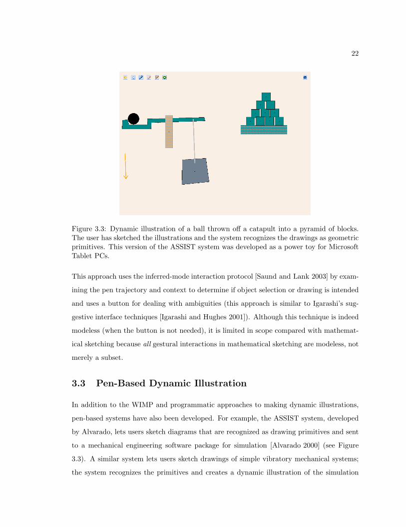
22
Figure 3.3: Dynamic illustration of a ball thrown off a catapult into a pyramid of blocks.The user has sketched the illustrations and the system recognizes the drawings as geometricprimitives. This version of the ASSIST system was developed as a power toy for MicrosoftTablet PCs.
This approach uses the inferred-mode interaction protocol [Saund and Lank 2003] by exam-
ining the pen trajectory and context to determine if object selection or drawing is intended
and uses a button for dealing with ambiguities (this approach is similar to Igarashi’s sug-
gestive interface techniques [Igarashi and Hughes 2001]). Although this technique is indeed
modeless (when the button is not needed), it is limited in scope compared with mathemat-
ical sketching because all gestural interactions in mathematical sketching are modeless, not
merely a subset.
3.3 Pen-Based Dynamic Illustration
In addition to the WIMP and programmatic approaches to making dynamic illustrations,
pen-based systems have also been developed. For example, the ASSIST system, developed
by Alvarado, lets users sketch diagrams that are recognized as drawing primitives and sent
to a mechanical engineering software package for simulation [Alvarado 2000] (see Figure
3.3). A similar system lets users sketch drawings of simple vibratory mechanical systems;
the system recognizes the primitives and creates a dynamic illustration of the simulation

23
[Kara et al. 2004].
The key to these systems is that they use domain knowledge about Newtonian mechanics
and recognize users’ sketches as specific primitives. Thus, although these systems provide
powerful illustrations of physics and mathematics concepts, they are limited in their domain
knowledge and in hiding the underlying mathematical formulations from the user. Since
mathematical sketching uses mathematics as its primary method of telling the system how
drawings should behave, our approach is more general and users can create more types of
dynamic illustrations.
Pen-based systems have also been developed for other types of dynamic illustration. For
example, Pickering et al. developed a system for sketching football plays, simulating them,
and then creating a dynamic illustration of the play outcome [Pickering et al. 1999]. Other
pen-based systems have been developed for creating traditional animations [Davis et al. 2003,
Davis and Landay 2004, Moscovich and Hughes 2004].
3.4 Computational and Symbolic Math Engines
The primary focus of mathematical software systems such as MathematicaTM, MapleTM,
MathCadTM, and MatlabTM has been entering mathematics for computation, symbolic
mathematics, and illustration. Graphing calculators and the myriad of educational math
software applications (see Tall [Tall 1987] for some examples) can be considered smaller
versions of these systems. These tools can create dynamic illustrations using mathematics
as input. However, the mathematical notation used in these systems is one-dimensional,
requiring unconventional notation for concepts that would be intuitive in 2D handwritten
mathematics. In addition, these systems do not let the user create diagrams in a natural
pencil-and-paper style.
3.5 Mathematical Expression Recognition and Applications
Finally, there has been a significant amount of work in mathematical expression recog-
nition systems that let users enter 2D handwritten mathematics [Chan and Yeung 2000b,
Matsakis 1999, Miller and Viola 1998, Zanibbi et al. 2002] (see Chapters 5 and 6 for a more

24
thorough review). Work in this area began as early as the mid-1960s with expression
recognition systems and algorithms developed by Anderson [Anderson 1968] and Martin
[Martin 1967]. However, only a few of these systems go beyond just developing recognition
technology. For example, Chan and Yeung [Chan and Yeung 2001a] developed a simple
pen-based calculator, while xThink, Inc. developed MathJournalTM, a system designed to
solve equations, perform symbolic manipulation, and make graphs. MathJournal is the
closest in spirit to mathematical sketching because its animation controls let users write
down and recognize mathematics, make drawings, and assign the mathematics to the draw-
ings.1 However, a key limitation of MathJournal’s animation control is that users must
keyframe their animations (typically providing a starting and ending frame), making the
user interface less fluid and contravening how users would make diagrams with pencil and
paper. In addition, MathJournal’s animation control lacks the iteration and conditional
constructs, diagram rectification, and modeless gestural user interface that mathematical
sketching supports.
1This functionality did not emerge till after mathematical sketching [LaViola and Zeleznik 2004] was firstpublished.

Chapter 4
A User Interface for Mathematical
Sketching
A modeless gestural user interface is a key component of mathematical sketching. Here we
describe the various components of the mathematical sketching user interface, discuss how
it was made modeless, and present some technical details.
4.1 Design Goals and Strategy
An important goal of mathematical sketching (see Figure 4.1) is to facilitate mathematical
problem solving without imposing any interaction burden beyond those traditional media.
Since pencil-and-paper users switch fluidly between writing equations and drawing sup-
porting diagrams, a modeless interface is highly desirable. Although a simple freehand
drawing pen would suffice to mimic pencil and paper, we want to support computational
activities including formula manipulation, diagram rectification (see Section 7.4), and ani-
mation. This functionality requires extending the notion of a freehand pen, either implicitly
by parsing the user’s 2D input on the fly or explicitly by letting the user perform gestural
operations. We chose an interface that combines both, in an effort to reduce the complexity
and ambiguities that arise in many hand-drawn mathematical sketches — we use parsing
to recognize mathematical expressions and make associations, and use gestures to segment
expressions and perform various symbolic and computational operations.
25

26
Figure 4.1: A mathematical sketch exploring damped harmonic oscillation shows a drawingof a spring and mass and the necessary equations for animating the drawing. The labelinside the mass associates the mathematics with the drawing.
The challenge then for mathematical sketching’s gestural user interface is that its ges-
tures not interfere with the entry of drawings or equations and still be direct and natural
enough to feel fluid. We utilize a threefold strategy to accomplish this task. First, we
use context sensitivity to determine what operations to perform with a single gesture.
Second, we use location-aware gestures so that a single gesture can invoke different com-
mands based on its location and size. Third, we use the notion of punctuated gestures
[Zeleznik et al. 2004], compound gestures with one or more strokes and terminal punctua-
tion, to help resolve ambiguities among gestures, mathematics and drawings. Combining
these techniques lets the entire interface be completely modeless and also lets us reduce the
gesture set while maintaining a high level of functionality.
One of the important issues is whether the gestures actually make sense, since a com-
pletely modeless user interface with a poor gesture set may not work well. Our gesture set
was chosen (see Figure 4.2 for a summary) using two important criteria. First, we wanted

27
Figure 4.2: Mathematical sketching gestures. Gesture strokes in the first column are shownhere in red. In the second column, cyan-highlighted strokes provide association feedback(the highlighting color changes each time a new association is made), and magenta strokesshow nail and angle association/rectification feedback.

28
our gestures to be easy to perform and learn. Second, we wanted gestures that work and
seem logical for multiple commands to be used for all those commands. For example, if
a particular gesture makes sense for two or three different operations, then we want that
gesture to invoke all those operations. This approach eases learning as well, since users
need not remember additional gestures. Chapter 10 describes a usability study on how
users perform with our gesture set, and shows they found them relatively easy to use and
remember.
4.2 Writing Mathematical Expressions
Writing mathematical expressions is the first of the three main parts of the mathematical
sketching user interface. It involves not only writing down the expressions but recognizing
them and correcting recognition mistakes.
We now introduce some notation used throughout this dissertation. Gestures are made
up of one more more digital ink strokes. A stroke is defined as a sequence of points in the
xy-plane
s = p1p2...pn (4.1)
where pi = (xi, yi), 1 ≤ i ≤ n, p1 is the pen-down point, pn is the pen-up point, and n is
the number of points in the stroke. A gesture is then a sequence of strokes
g = s1s2...sm (4.2)
where m is the number of strokes in the gesture. We also define a mathematical symbol as
a sequence of strokes
S = s1s2...sm (4.3)
where m is the number of strokes in the symbol.

29
4.2.1 Inking
Writing mathematical expressions in mathematical sketching is straightforward: users draw
with a stylus as they would with pencil and paper. The only complication in writing
expressions is how errant strokes are corrected. Although the stylus can be flipped over to
use its eraser, we found that a gestural action not requiring flipping was both more accurate
(because of hardware characteristics of the stylus) and more convenient. We therefore first
designed a scribble erase gesture in which the user scribbles with the pen back and forth
over the ink strokes to be deleted. However, this first implementation created too many false
positives: it recognized scribble erase gestures when in fact the user had intended to draw
ink and not erase anything. To alleviate this problem we settled on a punctuated gesture
because of its relative simplicity and ease of execution (see Figure 4.3). Thus our current
definition of scribble erase is the scribble stroke followed directly by a tap. In practice, users
found this compound gesture easy to learn, effective in eliminating false positives, and not
significantly more difficult or slower than the simple scribble gesture.
Figure 4.3: Scribbling over ink strokes and making a tap (top) erases the ink underneaththe scribble gesture (bottom).
To recognize the scribble erase gesture, we check when users make a tap, defined as
a stroke si such that its bounding box’s width and height are less then εtap. We found a
reasonable value for εtap is 10 pixels: it allows some leeway when users tap, since in many
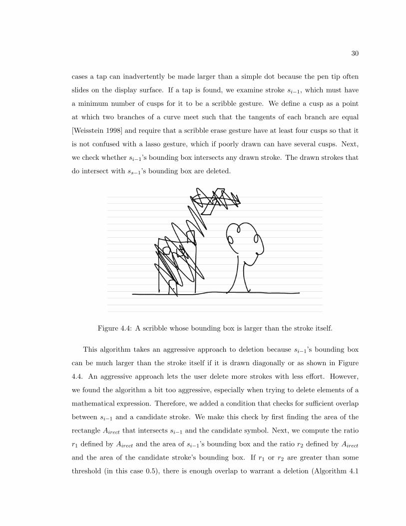
30
cases a tap can inadvertently be made larger than a simple dot because the pen tip often
slides on the display surface. If a tap is found, we examine stroke si−1, which must have
a minimum number of cusps for it to be a scribble gesture. We define a cusp as a point
at which two branches of a curve meet such that the tangents of each branch are equal
[Weisstein 1998] and require that a scribble erase gesture have at least four cusps so that it
is not confused with a lasso gesture, which if poorly drawn can have several cusps. Next,
we check whether si−1’s bounding box intersects any drawn stroke. The drawn strokes that
do intersect with ss−1’s bounding box are deleted.
Figure 4.4: A scribble whose bounding box is larger than the stroke itself.
This algorithm takes an aggressive approach to deletion because si−1’s bounding box
can be much larger than the stroke itself if it is drawn diagonally or as shown in Figure
4.4. An aggressive approach lets the user delete more strokes with less effort. However,
we found the algorithm a bit too aggressive, especially when trying to delete elements of a
mathematical expression. Therefore, we added a condition that checks for sufficient overlap
between si−1 and a candidate stroke. We make this check by first finding the area of the
rectangle Airect that intersects si−1 and the candidate symbol. Next, we compute the ratio
r1 defined by Airect and the area of si−1’s bounding box and the ratio r2 defined by Airect
and the area of the candidate stroke’s bounding box. If r1 or r2 are greater than some
threshold (in this case 0.5), there is enough overlap to warrant a deletion (Algorithm 4.1

31
gives a pseudocode description). This extra condition helps make our deletion strategy
less aggressive and worked well in practice. We could reduce the aggressiveness of our
deletion strategy even further by using convex hulls instead of bounding boxes, but this did
not seem necessary. See [Zeleznik et al. 2004] for more details on using convex hulls with
scribble erasing.
Algorithm 4.1 The scribble erase recognition algorithm.
Input: The tap stroke si, the scribble erase stroke si−1, a set of candidatestrokes CS = {s1, s2, . . . , sn}, and the tap threshold εtap.Output: A list of strokes L to be deleted. Note that L could be empty,indicating no deletion is needed.ScribbleErase(si,si−1,CS,εtap)(1) if Width(si) < εtap and Height(si) < εtap
(2) if Cusps(si−1) > 3(3) b1 ← BoundingBox(si−1)(4) foreach Stroke s ∈ CS(5) b2 ← BoundingBox(s)(6) b3 ← b1 ∩ b2
(7) if (s∩ b1) and (s 6= si−1) and (Area(b3)Area(b1) > 0.5 or
Area(b3)Area(b2) >
0.5)(8) L← s(9) return L
4.2.2 Recognizing Mathematical Expressions
Once mathematical expressions are drawn, they must be parsed by the system and converted
to strings for use by a computational engine. Our initial attempt, clicking on a Recognize
button that attempted to recognize all mathematics on the page, was problematic because
it was hard to algorithmically determine “lines of math” accurately, especially when the
expressions were closely spaced, at unusual scales or in unusual 2D arrangements. We
therefore chose a manual segmentation alternative by which users explicitly select a set of
strokes comprising a single mathematical expression by drawing a lasso. Since in a modeless
interface a lasso cannot be distinguished from a closed curve, we needed to disambiguate
these two actions. An approach that worked well for some people was to lasso lines of
math while pressing the barrel button on the stylus. However, many people inadvertently
triggered this button when trying to draw, while others found pressing a barrel button

32
awkward. Once again, the solution was to use punctuated gestures — this time drawing a
lasso around a line of mathematics followed by a tap inside the lasso (see Figure 4.5). We
chose to make the tap inside the lasso so we could perform other lasso-and-tap operations
described in Sections 4.3 and 4.4.1.
Figure 4.5: Mathematical expressions are recognized by drawing a lasso around them andmaking a tap inside the lasso (top). Recognized mathematics is shown in a red boundingbox (bottom).
As with the scribble erase gesture, we check when the user makes a tap with stroke si.
We then examine stroke si−1 to see if any drawn strokes are completely contained within
it (we can determine if a stroke is completely contained in si−1 with point-in-polygon algo-
rithms [Haines 1994]). Those strokes completely contained within the lasso are recognized
as mathematics. We made the restriction that strokes must be completely contained within
the lasso in order for them to be recognized so that we can reuse the lasso and tap for
making nails (see Section 4.3.1). The main problem with this constraint is that users some-
times make sloppy lassos that intersect strokes; in such cases, not all of the strokes will
be recognized. However, this problem occurs only infrequently and is easily corrected by
making another lasso and tap.
4.2.3 Feedback
Ideally, recognition would not require any feedback to users — the system would simply
understand what users had written. However, due to the complexity and ambiguities of
mathematical notation, it is essential that users know how mathematical sketching interprets
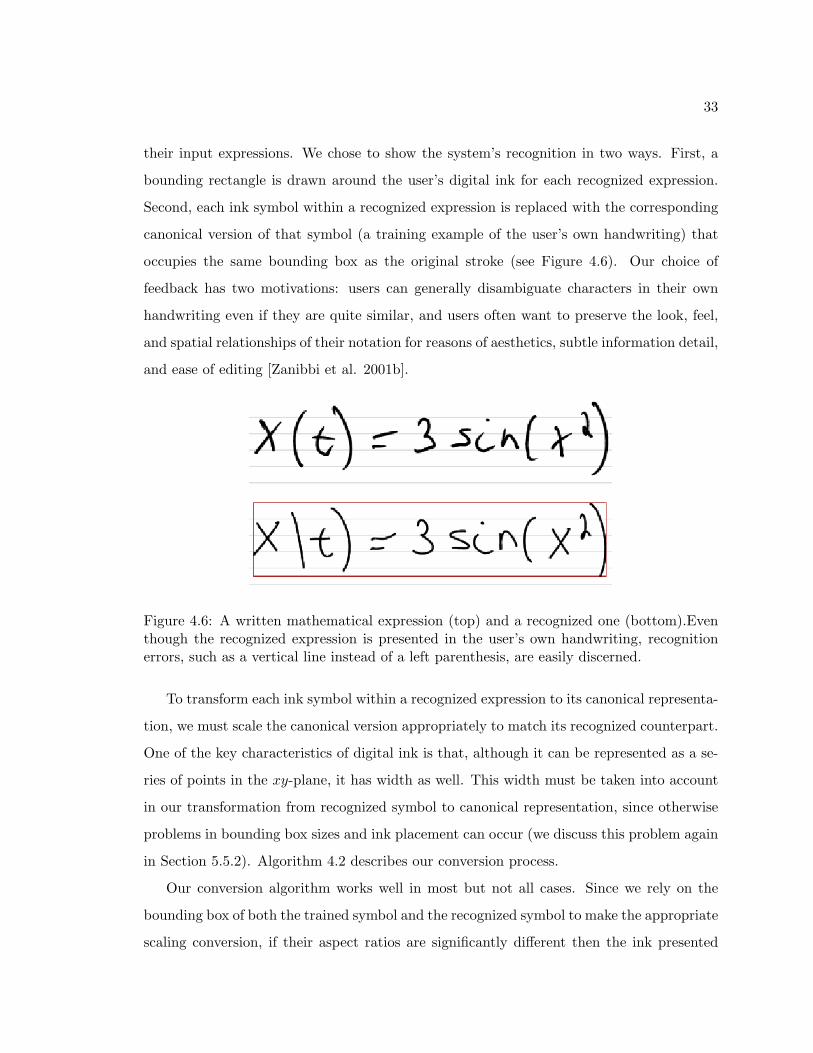
33
their input expressions. We chose to show the system’s recognition in two ways. First, a
bounding rectangle is drawn around the user’s digital ink for each recognized expression.
Second, each ink symbol within a recognized expression is replaced with the corresponding
canonical version of that symbol (a training example of the user’s own handwriting) that
occupies the same bounding box as the original stroke (see Figure 4.6). Our choice of
feedback has two motivations: users can generally disambiguate characters in their own
handwriting even if they are quite similar, and users often want to preserve the look, feel,
and spatial relationships of their notation for reasons of aesthetics, subtle information detail,
and ease of editing [Zanibbi et al. 2001b].
Figure 4.6: A written mathematical expression (top) and a recognized one (bottom).Eventhough the recognized expression is presented in the user’s own handwriting, recognitionerrors, such as a vertical line instead of a left parenthesis, are easily discerned.
To transform each ink symbol within a recognized expression to its canonical representa-
tion, we must scale the canonical version appropriately to match its recognized counterpart.
One of the key characteristics of digital ink is that, although it can be represented as a se-
ries of points in the xy-plane, it has width as well. This width must be taken into account
in our transformation from recognized symbol to canonical representation, since otherwise
problems in bounding box sizes and ink placement can occur (we discuss this problem again
in Section 5.5.2). Algorithm 4.2 describes our conversion process.
Our conversion algorithm works well in most but not all cases. Since we rely on the
bounding box of both the trained symbol and the recognized symbol to make the appropriate
scaling conversion, if their aspect ratios are significantly different then the ink presented

34
Algorithm 4.2 Transformation of recognized ink strokes to their canonical representationsin the user’s handwriting.
Input: Recognized ink symbol S = s1s2 . . . sn
Output: Converted ink symbol Snew
ConvertInkSymbol(S)(1) Sorig ← GetTrainingSetSymbolStrokes(S)(2) b1 ← BoundingBox(S)(3) penw = PenInkWidth()(4) b2 ← ResizeRectangleAboutCenter(b1,−penw/2)(5) xlow ← LowXCoord(b1)(6) ylow ← LowY Coord(b1)(7) xhi ← HighXCoord(b1)(8) yhi ← HighY Coord(b1)
(9) rw ← Width(b2)xhi−xlow
(10) rh ← Height(b2)yhi−ylow
(11) foreach Stroke s ∈ Sorig
(12) foreach Point (xi, yi) ∈ s(13) xi ← (xi − xlow)rw + UpperLeftCoordX(b2)(14) yi ← (yi − ylow)rh + UpperLeftCoordY (b2)(15) L← Point(xi, yi)(16) Snew ← L(17) return Snew
after recognition can be stretched too much or too little (see Figure 4.7). Square roots
are particularly problematic because they can be written with many different aspect ratios.
However, special-casing this symbol and stretching the top line fixes the problem. Similar
problems can arise with other symbols if they are written poorly or with odd dimensions,
and these cases would require a more general analysis of the symbol shapes. However, in
our experience, the current algorithm is sufficient since these other cases are rare.
Although we present the results of the symbol recognizer in the user’s own handwriting,
we do not currently provide a way to modify the layout of the recognized ink to correspond
to the 2D mathematical parse relationships; parsing feedback is currently provided in 1D.
Some users have expressed interest in a high-quality typeset feedback option to be used
primarily as an alternate view in a less technically interesting “clean-up” phase. While
this is a viable approach, in order to keep our pencil-and-paper aesthetic we are currently
investigating techniques for improved 2D layout constrained to the user’s input handwriting

35
Figure 4.7: What happens when the canonical symbol and recognized symbol have signif-icantly different aspect ratios. We special-case the square root symbol to deal with thisproblem.
style. Chapter 11 gives more details on presenting 2D parsing results.
4.2.4 Correcting Recognition Errors
Correcting recognition errors is very important in the mathematical sketching interface since
errors are bound to occur. If the per-symbol accuracy of a given recognizer is α, then the
accuracy of recognizing n symbols is αn. Thus, if α = 0.99 and our mathematical expression
has 15 symbols, the accuracy reduces to 86%, even ignoring parsing errors.
We can correct symbol recognition errors in two ways. First, users can tap on a rec-
ognized symbol to bring up a n-best list of alternatives for that symbol (see Figure 4.8);
when users click the correct symbol, the mathematical expression is updated both exter-
nally (in the user’s handwriting) and internally. Second, users can simply scribble erase
the offending symbols, rewrite them, and rerecognize the expression. Since we store each
recognized mathematical expression internally, the erasure of an offending symbol is noted
in the recognized expression’s data record. When the expression is rerecognized, only the
rewritten symbols are examined, making the operation fast and reliable.
In addition to correcting symbol recognition errors, users also need to correct parsing
errors arising when the mathematical expression recognizer has incorrectly determined the

36
Figure 4.8: A menu of symbol alternatives. Here, the user’s “2” in front of the x2 wasrecognized as an “h”. The user can correct the error by clicking on the first menu item.
relationship between symbols. One approach is to invoke a pull-down menu of expression
alternatives. When the stylus hovers over a recognized expression, a small green button
appears in the lower right corner of its bounding box. Pressing this button displays a menu of
alternative expressions and the display is updated to reflect the alternate expression selected
(see Figure 4.9).1 This pull-down menu works well when the expressions are small, but as
they become more complex generating useful alternatives becomes increasingly difficult,
since the number of parsing and symbol choices gets larger and larger. We discuss some
possible solutions to this problem in Chapter 11.
The second approach to correcting parsing mistakes is to let users move the mathemat-
ical symbols to new positions relative to the other symbols in the expression; when the user
finishes moving these symbols, the system automatically rerecognizes the expression. To
move a symbol or group of symbols, we use a lasso and drag gesture. Users first make a
lasso around the symbols of interest and then, starting inside the lasso, use the stylus to
drag the symbols to the desired location. This approach is very easy and makes intuitive
sense because a lasso says users want to operate on the selected symbols and dragging them
around is the most direct method for moving them. In addition, users find it convenient
1The first expression in this menu is the one the system thinks is correct and is used to see whether anyparsing mistakes have been made.

37
Figure 4.9: A menu of alternative expressions. The first menu item shows the recognizer’sinterpretation and the remaining menu items are the alternates. Here the system recognizedthe ink as y = xt2: the correct expression, y = xt2 , is the next-to-last menu item.
not only to correct parsing errors but also to manipulate terms.
The lasso and drag gesture is similar to the lasso and tap gesture for recognizing math-
ematical expressions; they differ in that the drag generates more ink than the tap does and
in that the lasso and drag is interactive. To recognize the lasso and drag gesture, we need to
know when a tap turns into a drag. In recognizing mathematical expressions, we examine
stroke si and, if it’s a tap, see whether si−1 is a lasso that contains any ink strokes. This
approach does not work with lasso and drag because we need to examine si in real time:
the best we could do is detect that si was a drag gesture and move the ink strokes contained
in si−1 to pn of si. This would cause the selected ink strokes to jump to the new location
instead of moving interactively.
Instead, we take a reverse approach: we determine whether si is a lasso that contains
recognized ink strokes. If the lasso contains recognized strokes, we examine stroke si+1 in
real time, inspecting each point as it is drawn. If the distance between point p1 and point
pi is greater than εdrag, some threshold (about 10 pixels) telling us si+1 could not be a tap,
then the ink strokes are interactively moved by pi+1 − pi until the end of the stroke. The
small jump that occurs with the first translation is minimal and not distracting to users.

38
4.3 Making Drawings
Diagrams are sketched in the same way as mathematical expressions except that the dia-
grams need not be recognized. In considering the value of a primitives-based drawing system
against the added interaction overhead of specifying primitives, we decided that our only
primitive would be unrecognized ink strokes. We believe that a primitives-based approach
would not only require a more elaborate user interface, but would also take away from the
pencil-and-paper aesthetic we want to achieve with mathematical sketching.
4.3.1 Nailing Diagram Components
In reviewing a broad range of mathematical illustrations, we found that the single low-
level behavior of stretching a diagram element can be very powerful. Thus, we support the
concept of “nails” to pin a diagram element to the background or pin a point on a diagram
element to another diagram element. If either diagram element is moved, the other element
either moves rigidly to stay attached at the nail (if it has only one nail) or stretches so that
all its nails maintain their points of attachment. Nails, although used primarily to create
non-rigid objects, can also create binary grouping relationships. We do not currently detect
or support cyclic nail relationships.
The user creates a nail by drawing a lasso around the appropriate location in the drawing
and making a tap gesture inside it (the tap disambiguates the nail gesture from a circle
that is part of a drawing). This lasso and tap gesture is the same as that used to recognize
mathematical expressions. Although we could have used other gestures, such as making a
lasso and writing the letter “N” (for nail) to create nails, lasso and tap seemed an attractively
more logical gesture since it is analogous to drawing the head of a nail and then hammering
it in with the tap.
As with the gestures for mathematical expression recognition, we detect if stroke si is a
tap and then examine stroke si−1. The key distinction between a nail lasso and a expression
recognition lasso concerns how it intersects with other drawing elements. A nail lasso must
intersect one or more drawing elements but cannot completely contain any of them; a lasso
that completely contains a drawing element is considered either a mathematical expression
recognition gesture or a grouping gesture (see Section 4.3.2), depending on tap location.

39
Figure 4.10: A nail gesture connecting the top line with the vertical line (left). A correctlyrecognized nail is indicated by a small red circle at the nail location (right).
The system links together all drawing elements that intersect the nail gesture’s lasso. The
link is then symbolized by centering a small red circle on the nail location (see Figure 4.10).
The center of the red circle is placed at the endpoint of one of the nail lasso’s intersected
strokes. If no endpoints are found, the nail lasso’s centroid is used.
4.3.2 Grouping Diagram Components
Since many drawings involve creating one logical object from a set of strokes (drawing
elements), we need to be able to group strokes into composite drawing elements. We can
use the same lasso gesture for a grouping operation by drawing a lasso around diagram
strokes. We can distinguish the grouping gesture on the basis of tap location. If stroke si is
a tap, we check whether stroke si−1 completely contains any drawn strokes. If the tap falls
within a few pixels of the lasso, then we perform a grouping operation (see Figure 4.11).
After the operation, a green box is drawn around the strokes to show that a grouping has
been made and to distinguish it from a recognized expression.
Although we could easily define a different gesture for grouping, we believe that main-
taining a simple contextually overloaded gesture set is easier for users than the alternative
larger gesture set. We explored overloading the mathematical expression recognition ges-
ture and determining whether to make a composite grouping or recognize mathematics by
classifying the strokes within a lasso as drawings or text. If the strokes are drawings, they
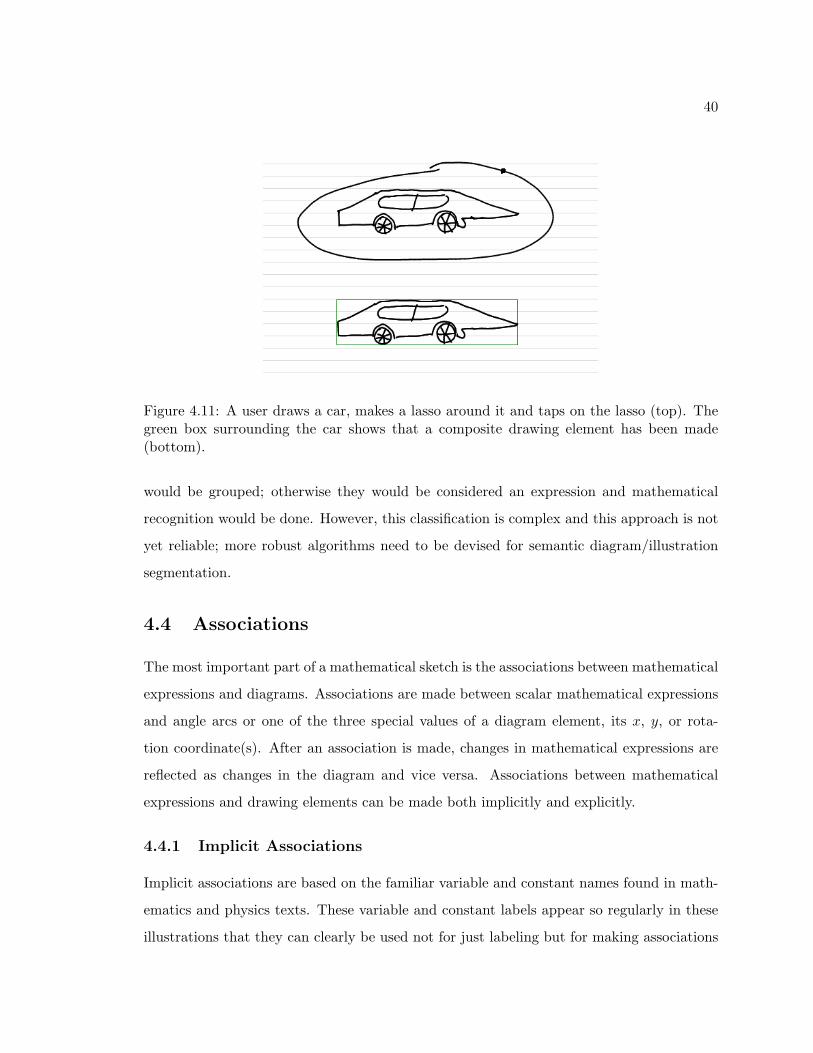
40
Figure 4.11: A user draws a car, makes a lasso around it and taps on the lasso (top). Thegreen box surrounding the car shows that a composite drawing element has been made(bottom).
would be grouped; otherwise they would be considered an expression and mathematical
recognition would be done. However, this classification is complex and this approach is not
yet reliable; more robust algorithms need to be devised for semantic diagram/illustration
segmentation.
4.4 Associations
The most important part of a mathematical sketch is the associations between mathematical
expressions and diagrams. Associations are made between scalar mathematical expressions
and angle arcs or one of the three special values of a diagram element, its x, y, or rota-
tion coordinate(s). After an association is made, changes in mathematical expressions are
reflected as changes in the diagram and vice versa. Associations between mathematical
expressions and drawing elements can be made both implicitly and explicitly.
4.4.1 Implicit Associations
Implicit associations are based on the familiar variable and constant names found in math-
ematics and physics texts. These variable and constant labels appear so regularly in these
illustrations that they can clearly be used not for just labeling but for making associations

41
Figure 4.12: Lassoing 50 and tapping on the horizontal line between the tree and housemakes an implicit point association (top). The expression and drawing element are high-lighted in a pastel color to indicate the association was made (bottom).
as well. Mathematical sketching supports point and angle associations implicitly and uses
the recognized label and linked drawing element to infer associations with other expressions
on the page (see Section 7.2).
To create an implicit point association, users draw a variable name or constant value
near the intended drawing element and then use the mathematical expression recognition
gesture to recognize the label. The tap location can have two meanings in completing
the point association. If the recognition gesture’s tap falls within its lasso, then the label
is linked to the closest drawing element within some global distance threshold (we use a
global distance threshold so that mathematical expressions a significant distance away from
a drawing element are not inadvertently associated to that element). If the tap location is
outside the lasso, it specifies both the drawing element to be linked to the label (see Figure
4.12) and the drawing element’s center of rotation (this point is used only for rotational
labels). Note that the tap must be located on the drawing element or in the bounding box
of a composite drawing element. We have found that users prefer tapping on the drawing
element rather than inside the lasso to make a point association, probably because they
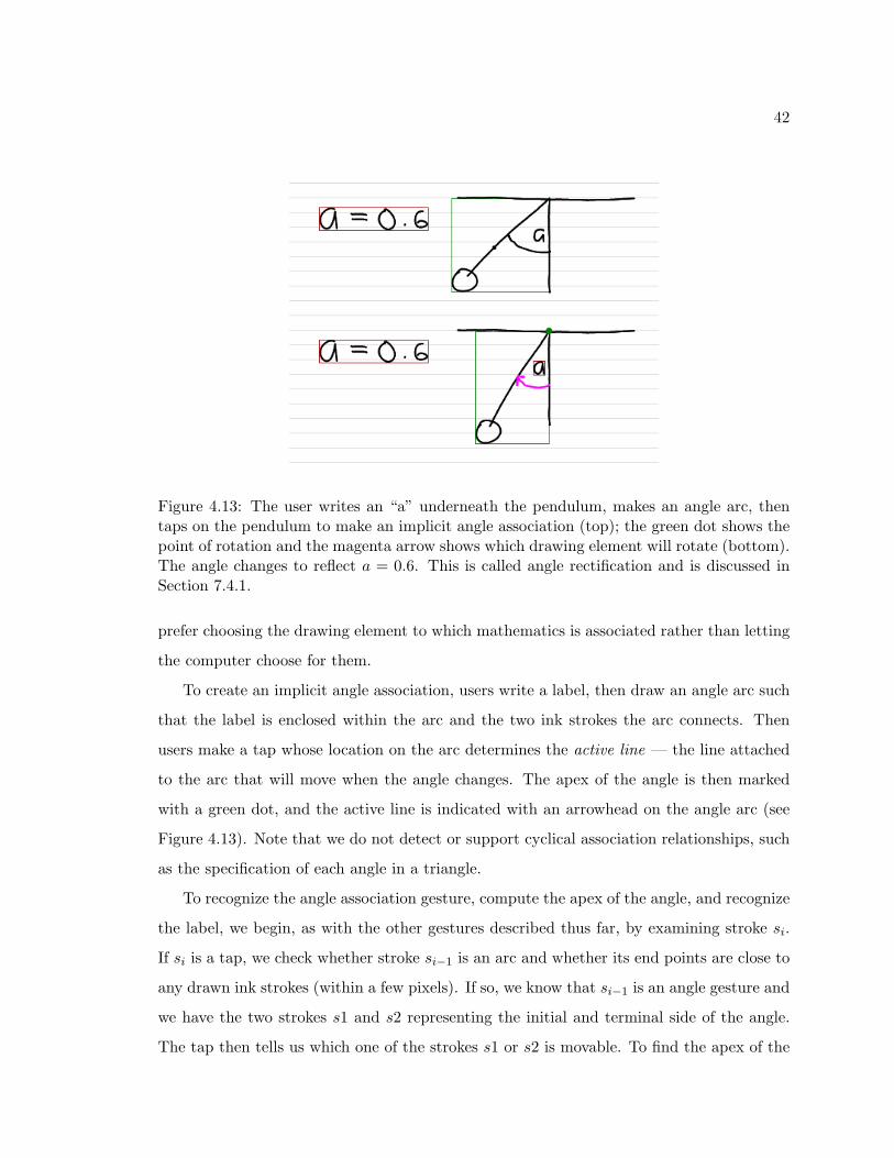
42
Figure 4.13: The user writes an “a” underneath the pendulum, makes an angle arc, thentaps on the pendulum to make an implicit angle association (top); the green dot shows thepoint of rotation and the magenta arrow shows which drawing element will rotate (bottom).The angle changes to reflect a = 0.6. This is called angle rectification and is discussed inSection 7.4.1.
prefer choosing the drawing element to which mathematics is associated rather than letting
the computer choose for them.
To create an implicit angle association, users write a label, then draw an angle arc such
that the label is enclosed within the arc and the two ink strokes the arc connects. Then
users make a tap whose location on the arc determines the active line — the line attached
to the arc that will move when the angle changes. The apex of the angle is then marked
with a green dot, and the active line is indicated with an arrowhead on the angle arc (see
Figure 4.13). Note that we do not detect or support cyclical association relationships, such
as the specification of each angle in a triangle.
To recognize the angle association gesture, compute the apex of the angle, and recognize
the label, we begin, as with the other gestures described thus far, by examining stroke si.
If si is a tap, we check whether stroke si−1 is an arc and whether its end points are close to
any drawn ink strokes (within a few pixels). If so, we know that si−1 is an angle gesture and
we have the two strokes s1 and s2 representing the initial and terminal side of the angle.
The tap then tells us which one of the strokes s1 or s2 is movable. To find the apex of the

43
Figure 4.14: A user draws a line through the mathematics; as the stylus hovers over theball, it turns cyan (top). With a tap, the mathematics is associated to the ball and ishighlighted along with the mathematics in a pastel color to confirm that the associationwas made (bottom).
angle, we find the intersection points closest to the end points of si−1 on s1 and s2 and use
these to create lines along s1 and s2 (we assume that s1 and s2 are close to linear near the
intersection points). We can then perform a line intersection test to find the apex. Using
the apex and si−1, we can then construct a polygon that tells us what ink strokes we should
send to the recognizer. Algorithms 4.3 – 4.5 summarize this approach.
4.4.2 Explicit Associations
For slightly more control over associations and to reduce the density of information in a
diagram, associations can also be created explicitly without using variable name labels.
The user makes an explicit association by drawing a line through a set of related mathe-
matical expressions and then tapping on a drawing element (see Figure 4.14). After this
line is drawn, drawing elements change color as the stylus hovers over them to indicate the
potential for an association. This technique provides greater flexibility than the implicit
association techniques in two ways. First, explicit associations can specify the precise point
of rotation: instead of just tapping on the drawing element (which sets the point of rotation

44
Algorithm 4.3 How implicit angle gestures are recognized.
Input: The tap stroke si, the angle stroke si−1, a set of candidate strokesCS = {s1, s2, . . . , sn}, the tap threshold εtap, and the radius r for the circletest.Output: True or FalseRecognizeAngleArc(si,si−1,CS,εtap,r)(1) if Width(si) < εtap and Height(si) < εtap
(2) b1 ← BoundingBox(si−1)(3) P ← Points(si−1)(4) slen ←
∑ni=2 ‖Pi − Pi−1‖
(5) blen ← 2 ·Width(b1) ·Height(b1)(6) if slen < blen and (s2
len > Width(b1)2 + Height(b1)
2)(7) c1 ← Circle(P1, r)(8) c2 ← Circle(P2, r)(9) is1← GetStrokeIntersectedWithCircle(c1, CS)(10) is2← GetStrokeIntersectedWithCircle(c2, CS)(11) if is1 and is2(12) return true(13) return false
Algorithm 4.4 Computes the angle apex. Note that part of this algorithm was adaptedfrom [Schneider and Eberly 2003]. We assume that the first point in si−1 is closest to sinit
and the last point in si−1 is closest to sterm.
Input: The angle stroke si−1, a set of candidate strokes CS ={s1, s2, . . . , sn}, the initial and terminal strokes sinit and sterm, and an indexvariable k used to construct the initial and terminal lines.Output: The apex point or null.ComputeApex(si−1,CS,sinit,sterm,k)(1) P1← Points(sinit)(2) P2← Points(sterm)(3) i1 ← NearestPointIndex(sinit, F irstPoint(si−1))(4) i2 ← NearestPointIndex(sterm, LastPoint(si−1))(5) d0 ← Point(X(P1i1+k)−X(P1i1−k), Y (P1i1+k)− Y (P1i1−k))(6) d1 ← Point(X(P2i2+k)−X(P2i2−k), Y (P2i2+k)− Y (P2i2−k))(7) e← P2i2−k − P1i1−k
(8) kross← X(d0)Y (d1)− Y (d0)X(d1)(9) ε← 0.001(10) if kross2 > ε · (X(d0)
2 + Y (d0)2)(X(d1)
2 + Y (d1)2)
(11) s← X(e)Y (d1)−Y (e)X(d1)kross
(12) return P1i1−k + s · d0
(13) return ∅

45
Algorithm 4.5 Finds the angle label’s ink strokes.
Input: The angle stroke si−1, a set of candidate strokes CS ={s1, s2, . . . , sn}, and the apex point ipt.Output: No return valueFindLabel(si−1,CS,ipt)(1) P ← Points(si−1)(2) p1 ← ipt(3) p2 ← P1
(4) p3 ← Pbn2c
(5) p4 ← Pn
(6) polyg ← Polygon(p1, p2, p3, p4)(7) foreach Stroke s ∈ CS(8) if s ⊂ polyg(9) Slist ← s(10) if Slist 6= ∅(11) Recognize(Slist)
at the center of the drawing element), users can press down on the element to select it,
move the stylus, and then lift the stylus to the desired center of rotation, even if it is not on
the drawing element. Second, explicit associations are somewhat faster than their implicit
counterparts because they do not require users to write down a label first. In addition,
users can make an association to a composite drawing element as a whole (e.g., a car) by
taping on empty space withing the composite’s bounding box, or to a part of the composite
(e.g., a wheel) by tapping directly on an ink stroke.
Recognizing explicit associations is somewhat different from what we seen thus far.
Technically, an explicit association is not a punctuated gesture, and thus we do not first
test whether stroke si is a tap. To recognize an explicit association gesture, si must meet
the following conditions:
• The first point in si must be inside the bounding box of a mathematical expression.
• The last point in si must be inside the bounding box of a mathematical expression.
• The stroke must not intersect itself.
• The stroke must have fewer than four cusps.

46
These conditions are required so there are no ambiguities with other gestures such as graph-
ing and solving equations (see Section 4.5) and scribble erase. If the conditions are met,
then the next stroke si+1 completes the association based on its location relative to the
drawing elements written on the page. In our experience, most users have little trouble
making smooth lines that fit the above criteria.
With both implicit and explicit associations, mathematical sketching provides an option
for visualizing the associations of drawing elements, labels, and expressions by filling the
bounding boxes of all associated components with the same semi-transparent pastel color.
4.5 Supporting Mathematical Toolset
Mathematical sketching also supports mathematical tools for graphing, solving, simplifying,
and evaluating recognized functions and equations. The utility of this toolset is twofold.
First, it provides traditional tools found in other software packages, so that mathematical
sketching becomes a more complete problem-solving and visualization approach. Second,
these tools can help in creating mathematical sketches, for example, solving a differential
equation to obtain the equations of motion for a sketch or integrating F = ma to find
velocity as a function of time.
4.5.1 Graphing Equations
Users can graph recognized functions with a simple line gesture that begins on the function
and ends at the graph’s intended location. The graphing gesture is essentially the same
as that used for creating explicit associations, except that it must have a minimum length
and its end point must fall outside any of recognized expressions’ bounding boxes. The
graphing gesture (see Figure 4.15) must have a minimum length (about 160 pixels) so that
it is not interpreted as a mathematical symbol such as a fraction line. A nice feature of
this gesture is that it lets users graph more than one function at a time by making sure
that any part of the gesture line (except the end point) intersects an expression’s bounding
box. The graphing gesture produces a movable, resizable graph widget displaying a plot of
the function. Additional graph gestures that end on this widget will overlay or replace the
function being graphed, depending on the state of the “hold plot” check box in the upper

47
Figure 4.15: A graphing gesture (top) that graphs all three recognized functions and plotsthem in a graph widget (bottom).
left corner of the widget.
The graph widget uses default values for the domain of plotted functions based on a
very simple heuristic: the domain is 0...5 for functions of t and −5...5 for functions of any
other variable. Users can override these defaults by including a domain when they write a
mathematical function. For example, to graph the function y = cos(ex) from 2 to 12, users
could write y = cos(ex), x = 2 . . . 12. Once the function is plotted, the domain or range can
be changed by selecting a region of the graph to zoom in on or by writing a new value below
the start or end of the graph and then clicking the update button. In choosing between
writing the domain of a function explicitly and changing the domain once it’s plotted in
the graph widget, users tend to prefer the latter since, in general, it is a faster operation.
Note that optional visual feedback can show correspondences between a plot line and a
mathematical expression by coloring the line in the same color as the expression bounding
boxes (see Figure 4.16).

48
Figure 4.16: Two plots created using graph gestures. Expression bounding boxes are coloredto correspond to plot lines.
4.5.2 Solving Equations
Mathematical sketching also lets users solve equations. The solver is invoked by a squiggle
gesture (see Figure 4.17)2 that resembles the graphing gesture in that its start point must be
inside a recognized expression’s bounding box, its end point must be outside all expression
bounding boxes, and it can intersect multiple recognized expressions along the way. Its
distinguishing characteristic is that it must have two self-intersections whereas the graphing
gesture must have none. We could have overloaded the graphing gesture and then examined
the context of the intersected recognized expressions to determine whether a graphing or
solving operation was intended, but it makes more sense to have two distinct gestures for
these tasks since graphing and solving are two distinct operations. The squiggle gesture is
somewhat arbitrary but users have found it easy to remember and perform. Once a squiggle
gesture is recognized, the system presents the solution to users at the end of the gesture.
2The output generated from equation solving and expression evaluation is taken directly from Matlab(our computational engine) syntax. We plan on presenting this output in the user’s own handwriting infuture versions of mathematical sketching.

49
Figure 4.17: A squiggle gesture through three equations (left), and the results of the simul-taneous equation solve (right).
Users can solve single equations, simultaneous equations, and ordinary differential equa-
tions (with and without initial conditions) using the same squiggle gesture. When a squiggle
gesture is made, the recognized equations intersected by that gesture are examined to deter-
mine what type of solving routine to perform. If there is only one recognized equation and
it has no derivatives, then we call a single equation solver. If the equation contains deriva-
tives, we call an ordinary differential equation solver. If more than one recognized equation
are intersected, we check whether any derivatives are present. If so, the other equations
are examined to see if they give valid initial conditions for the differential equation. If so,
we call an ordinary differential equation solver (see Figure 4.18). If none of the recognized
equations have derivatives, then we call a simultaneous equation solver (we also support
simultaneous ordinary differential equations). With this approach users need to remember
only one gesture, making the interface much simpler.
4.5.3 Evaluating Expressions
A variety of different mathematical expressions can be evaluated using the supporting
toolset. To evaluate a recognized expression, users make an equal sign and then a tap
inside the equal sign’s bounding box on the right side of the expression (see Figure 4.19).
Choosing an equal sign as part of our evaluation gesture is logical for these types of oper-
ations since users are looking for equivalent mathematical expression representations. In
addition, equal is one of the most common mathematical symbols and has an understood
meaning.

50
Figure 4.18: The results of a ordinary differential equation solve on a second-order differ-ential equation with initial condition.
Algorithm 4.6 Determines if two strokes make up an equal sign. Note we use 1.5 for ourbounding box threshold and 15 pixels for our line difference threshold.
Input: Strokes si−1 and si−2, a bounding box threshold εbox, and a linedifference threshold εdiff .Output: True or false.DetectEqualSign(si−1,si−2,εbox,εdiff )(1) P ← Points(si−1)(2) Q← Points(si−2)(3) b1 ← BoundingBox(si−1)(4) b2 ← BoundingBox(si−2)(5) slen1 ←
∑ni=2 ‖Pi − Pi−1‖
(6) slen2 ←∑n
i=2 ‖Qi −Qi−1‖(7) if slen1 > εbox
√
Width(b1)2 + Height(b1)2 or slen2 >εbox
√
Width(b2)2 + Height(b2)2
(8) return false(9) if Width(b1) < Height(b1) or Width(b2) < Height(b2)(10) return false(11) diff 1 = |X(P1)−X(Q1)|(12) diff 2 = |X(Pn)−X(Qn)|(13) if LineOverlap(P1, Pn, Q1, Qn) and diff 1 < εdiff and diff 2 < εdiff(14) return true(15) else
(16) return false

51
Figure 4.19: A user evaluates an expression using an equal tap gesture (top), yielding asimplification of the expression (bottom).
Figure 4.20: A variety of expressions evaluated using the equal tap gesture.
An equal and tap gesture is recognized by examining stroke si to check if it is a tap.
If so, we check whether an equal sign is present and the tap is inside its bounding box.
An equal sign is recognized by examining strokes si−1 and si−2 to see if they are small,
approximately straight horizontal lines of roughly the same length. If so, the evaluation is
performed. Algorithm 4.6 summarizes the equal detection procedure.
As in solving equations, the recognized mathematical expression to the left of the equal
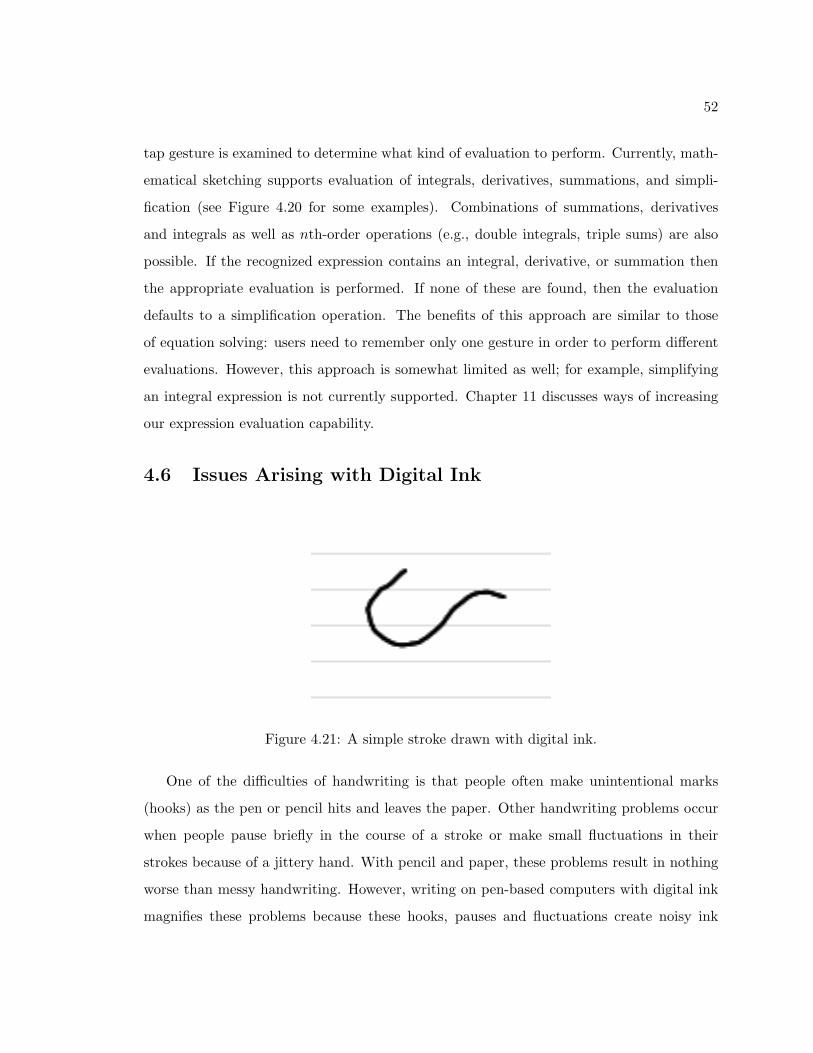
52
tap gesture is examined to determine what kind of evaluation to perform. Currently, math-
ematical sketching supports evaluation of integrals, derivatives, summations, and simpli-
fication (see Figure 4.20 for some examples). Combinations of summations, derivatives
and integrals as well as nth-order operations (e.g., double integrals, triple sums) are also
possible. If the recognized expression contains an integral, derivative, or summation then
the appropriate evaluation is performed. If none of these are found, then the evaluation
defaults to a simplification operation. The benefits of this approach are similar to those
of equation solving: users need to remember only one gesture in order to perform different
evaluations. However, this approach is somewhat limited as well; for example, simplifying
an integral expression is not currently supported. Chapter 11 discusses ways of increasing
our expression evaluation capability.
4.6 Issues Arising with Digital Ink
Figure 4.21: A simple stroke drawn with digital ink.
One of the difficulties of handwriting is that people often make unintentional marks
(hooks) as the pen or pencil hits and leaves the paper. Other handwriting problems occur
when people pause briefly in the course of a stroke or make small fluctuations in their
strokes because of a jittery hand. With pencil and paper, these problems result in nothing
worse than messy handwriting. However, writing on pen-based computers with digital ink
magnifies these problems because these hooks, pauses and fluctuations create noisy ink
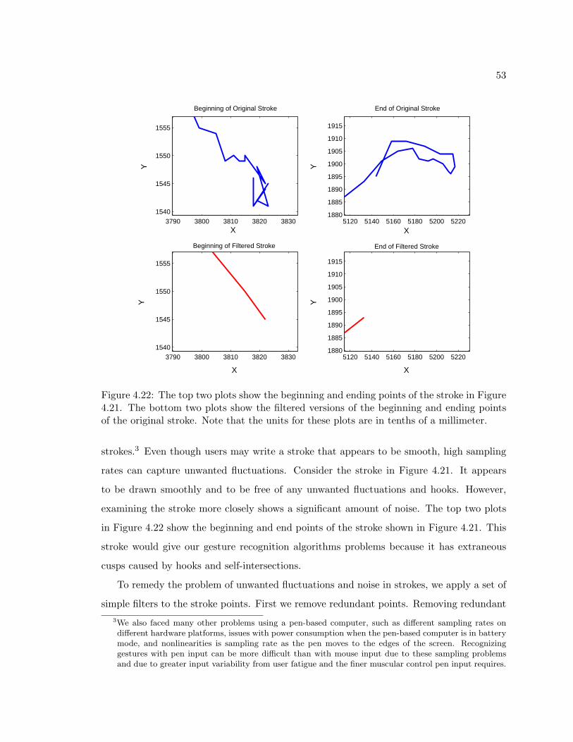
53
3790 3800 3810 3820 38301540
1545
1550
1555
X
Y
Beginning of Original Stroke
5120 5140 5160 5180 5200 52201880
1885
1890
1895
1900
1905
1910
1915
X
Y
End of Original Stroke
3790 3800 3810 3820 38301540
1545
1550
1555
Beginning of Filtered Stroke
X
Y
5120 5140 5160 5180 5200 52201880
1885
1890
1895
1900
1905
1910
1915
X
Y
End of Filtered Stroke
Figure 4.22: The top two plots show the beginning and ending points of the stroke in Figure4.21. The bottom two plots show the filtered versions of the beginning and ending pointsof the original stroke. Note that the units for these plots are in tenths of a millimeter.
strokes.3 Even though users may write a stroke that appears to be smooth, high sampling
rates can capture unwanted fluctuations. Consider the stroke in Figure 4.21. It appears
to be drawn smoothly and to be free of any unwanted fluctuations and hooks. However,
examining the stroke more closely shows a significant amount of noise. The top two plots
in Figure 4.22 show the beginning and end points of the stroke shown in Figure 4.21. This
stroke would give our gesture recognition algorithms problems because it has extraneous
cusps caused by hooks and self-intersections.
To remedy the problem of unwanted fluctuations and noise in strokes, we apply a set of
simple filters to the stroke points. First we remove redundant points. Removing redundant
3We also faced many other problems using a pen-based computer, such as different sampling rates ondifferent hardware platforms, issues with power consumption when the pen-based computer is in batterymode, and nonlinearities is sampling rate as the pen moves to the edges of the screen. Recognizinggestures with pen input can be more difficult than with mouse input due to these sampling problemsand due to greater input variability from user fatigue and the finer muscular control pen input requires.

54
Algorithm 4.7 Filters ink strokes to remove redundant points and unwanted self-intersections. Note that we use 5 pixels for our self-intersection threshold.
Input: Stroke si and a self-intersection threshold α.Output: A filtered list of pointsFilterStroke(si,α)(1) P ← Points(si)(2) curpt ← P1
(3) for i = 2 to n(4) if curpt = Pi
(5) BadPts← Pi
(6) else
(7) curpt = Pi
(8) RemovePointsFromPointList(BadPts, P )(9) SelfInts← SelfIntersectionLocations(P )(10) prev ← −1(11) for i = 1 to ‖P‖(12) if prev 6= −1 and SelfIntsi − prev > α(13) for j = prev to SelfIntsi
(14) BadPts← Pj
(15) prev ← SelfIntsi
(16) RemovePointsFromPointList(BadPts, P )(17) return P
points is important because when users write a stroke slowly or pause for a bit, the samples
still being generated can cause noise and repeated points in the ink stroke. Second, we
examine all self-intersections and remove those that are small (contained within five pixels).
These unwanted self-intersections can be caused from redundant points or can be function
of how slowly users draw the stroke. For example, these unwanted self-intersections can be
created at the beginning of the stroke when users unknowingly draw over the initial stroke
point. Finally, we apply a dehooking algorithm to the beginning and end of the stroke.
Unfortunately, even at low sampling rates, hooks are a natural phenomenon in writing and
can cause unwanted cusps and self-intersections as well. The dehooking algorithm looks for
increasing changes in stroke length from point p1 to pi up to a threshold (about five pixels);
when the length gets smaller than the maximum distance found, the points up to that
decreased length are removed. A summary of our filtering approach is shown in Algorithms
4.7 and 4.8.
Note that the amount of noise introduced into any given stroke is system dependent, so

55
Algorithm 4.8 Dehooking an ink stroke. Note we use 15 pixels for the minimum hookthreshold, 20 pixels for the maximum hook threshold, and 5 pixels for the dehooking distancethreshold.
Input: Stroke si, minimum and maximum hook threshold hookmin andhookmax, and a dehooking distance threshold εhook.Output: A dehooked list of pointsDeHook(si,hookmin,hookmax,εhook)(1) P ← Points(si)(2) maxdist← 0(3) for i = 2 to min(hookmin, Pn − hookmax)(4) dist← ‖Pi − P1‖(5) if dist > εhook
(6) break
(7) if dist ≥ maxdist(8) maxdist = dist(9) else
(10) for j = 1 to i(11) BadPts← Pj
(12) break
(13) maxdist← 0(14) for i = Pn−1 down to max(hookmax, Pn − hookmin)(15) dist← ‖Pn − Pi‖(16) if dist > εhook
(17) break
(18) if dist ≥ maxdist(19) maxdist = dist(20) else
(21) for j = n down to i(22) BadPts← Pj
(23) break
(24) RemovePointsFromPointList(BadPts, P )(25) return P
that the level of filtering needed often depends on the hardware. Also, the various constants
values were chosen empirically based on pilot user trials. Unfortunately, people often make
hooks of varying sizes, so that it is difficult to come up with robust constants. On the
basis of user trials, however, our filtering approach works well in removing unwanted self-
intersections and redundant points, making our gesture recognition robust across a variety
of writing styles and dynamics. The dehooking algorithm also works well but sometimes
removes too much of a stroke. However, in our experience, this aggressiveness does not

56
hamper the gesture recognition algorithms: most users find it easy to invoke the various
gestural commands that mathematical sketching provides.

Chapter 5
Mathematical Symbol Recognition
According to the definition of mathematical sketching, users write mathematical expres-
sions as part of the dynamic illustration process. These handwritten expressions must be
recognized so they can be used later in specifying the behavior of a drawing element or in
a computational or symbolic operation. This chapter focuses on the first part of the math-
ematical expression recognition problem (mathematical symbol recognition) and describes
our symbol recognition engine.
5.1 The Problem
According to Blostein and Grbavec [Blostein and Grbavec 1997], mathematical expression
recognition has the following six components:
1. early processing
2. symbol segmentation
3. symbol recognition
4. identification of spatial relationships among symbols
5. identification of logical relationships among symbols
6. construction of meaning
57

58
We focus on the first three components in this chapter and discuss our solutions to the last
three in Chapter 6.
The first three components of mathematical expression recognition (i.e., mathematical
symbol recognition) are not just simple independent processes: they have an important
interdependence. To perform mathematical symbol recognition, the ink strokes must be
segmented into symbols, and before that they must undergo preprocessing to ensure invari-
ance and reduce noise. More detail on preprocessing and symbol segmentation is given in
Sections 5.5.1 and 5.5.2.
Mathematical symbol recognition for pen-based input entails collecting a group of ink
strokes, determining which strokes constitute a symbol, and classifying those strokes as
one of a set of symbols defined by some alphabet. In addition, we must ensure that users
can write these symbols in any size and location on a digitizing surface without regard
to hand jitter and noise. More formally, for a set of ink strokes (written in any order)
s = {s1, s2, ..., sn}, we create a partition S such that Si 6= ∅, Si ∩ Sj = ∅ ∀i 6= j, and⋃
i Si = s. We then wish to classify each Si ∈ S such that Si ∈ A, where A = {c1, c2, ..., cm}is a set of symbols and m is the number of symbols in the alphabet.
5.2 Previous Work in Mathematical Symbol Recognition
Much work has been done in mathematical symbol as well as general character recog-
nition. We restrict ourselves to describing some of the more common approaches; more
thorough reviews can be found in [Chan and Yeung 2000b, Plamondon and Srihari 2000,
Tappert et al. 1990].
The key to recognizing symbols is to create a unique representation for a symbol that
can be used to classify it as one of the symbols in an alphabet. These representations can
then used as input to a classification algorithm. One of the first approaches to symbol
recognition was to break symbols up into zones based on the symbol’s bounding box. The
sequence of zones traversed by the stylus was used to identify the symbol [Day et al. 1972,
Donahey 1976]. Similarly, pen motion based on direction sequences has been used with
lookup tables to recognize symbols [Groner 1968, Powers 1973].

59
One of the most common approaches is to use feature analysis: various statistical and ge-
ometric measures calculated from the candidate symbol are used to derive separable charac-
teristics from them. Computed features can be as simple as whether a symbol is an ascender
or descender [Hanaki and Yamazaki 1980] or more complex, such as the symbol’s Fourier co-
efficients [Impedovo et al. 1978]. Smithies [Smithies et al. 1999] and Rubine [Rubine 1991]
both use a variety of statistical and geometric features (angle and quadrant histograms, as-
pect ratio, stroke length, and others) as input to a K-means classifier and a simple linear clas-
sifier, respectively. Features can be used as input to other classification algorithms as well,
including template matching [Connell and Jain 2000, Littin 1995, Miller and Viola 1998,
Nakayama 1993], decision trees [Belaid and Haton 1984, Kerrick and Bovik 1988], neural
networks [Dimitriadis and Coronado 1995, Marzinkewitsch 1991], hidden Markov models
[Koschinski et al. 1995, Kosmala and Rigoll 1998, Winkler 1994], support vector machines
[Bahlmann et al. 2002], and Gaussian classifiers with principal component analysis (PCA)
[Matsakis 1999].
Another common approach to symbol recognition is curve matching, which uses the
symbol’s strokes rather than features computed from them. In general, the strokes from a
candidate symbol are matched with those from a set of prototype curves and the closest
match identifies the candidate. In most cases the curves that are matched are functions
of time, such as the x and y values of a symbol [Odaka et al. 1982]. One of the ma-
jor drawbacks of curve matching is that curves from one symbol to another may have
a different number of points, making the best fit a nonlinear matching. These types of
sequence-comparison problems utilize a more flexible version of curve matching called elas-
tic matching [Chan and Yeung 1998a, Dimitriadis and Coronado 1995, Li and Yeung 1997,
Scattolin and Krzyzak 1994, Vuokko et al. 1999].
Other types of symbol recognition techniques include motor models and primitive de-
composition. Motor models, which have to do with how handwriting is generated, have
been used to analyze stroke segments; segments are then used along with rules on how
they are connected to recognize symbols [Plamondon and Maarse 1989]. Primitive decom-
position, another approach for recognizing symbols, is based on breaking strokes into com-
mon building blocks such as lines, loops, dots, and curves. Symbols broken down into

60
these building blocks are then used as templates for recognition [Chan and Yeung 1998a,
Xuejun et al. 1997].
5.3 Writer Dependence and The Training Application
One of the most important decisions in designing a mathematical symbol recognition en-
gine is whether it should be writer-independent or writer-dependent. Each approach has
advantages and disadvantages. The clear advantage of writer-independent systems is that
users need not train the recognizer beforehand: they can simply step up to the application
and start writing. However, writer-independent systems also have some significant limita-
tions from both a usability and a design perspective: recognition accuracy tends to suffer
because the recognition engine must accommodate a variety of different handwriting styles.
The goal of a writer-independent system is often to let anyone use the system easily, but
not necessarily to maximize accuracy for any one particular individual. Therefore, users
working with writer-independent systems often adapt their handwriting to the recognizer to
improve accuracy. From a design point of view, the recognizer still needs training data; in
fact, in order to be writer-independent, significantly more training data is required to obtain
a general and robust recognizer. Thus, the writer-independent system is writer-dependent
to a certain extent. Of course, once enough data has been obtained, training is no longer
needed (unless the recognizer is adaptive).
With a writer-dependent system, each user must train the recognizer with samples from
his or her handwriting. Therefore, one of the major disadvantages of a writer-dependent
system is the startup costs required to get users ready to use the recognizer: depending on
how many handwriting samples are needed, it can take several hours to train the recog-
nizer on a particular person’s handwriting. Although these startup costs are a limitation of
writer-dependent systems, writer dependence has some important advantages. Writer de-
pendence allows personalized recognizers tailored toward a particular user. In general, such
recognizers obtain higher recognition accuracy since they need deal with only one user’s
writing style at a time and can be fine-tuned to the way users write certain symbols. Note,
however, that in some cases writer-dependent systems are not truly writer-dependent. Con-
sider the symbols in Figure 5.1. The 1 in 12 and l in log are essentially indistinguishable

61
Figure 5.1: The 1 in 12 and the l in log are indistinguishable.
without context, and even with context, it can be almost impossible to distinguish between
them. Users who write their 1’s and l’s in this manner will have to write one of them differ-
ently so that the recognizer has a chance of distinguishing between the two. Therefore, in
some cases, users must adapt their handwriting even with a writing-dependent recognizer.
5.3.1 User Training
We chose a writer-dependent symbol recognizer for several reasons. First, we wanted the
highest accuracy possible and felt that having each user train the recognizer would enhance
accuracy. Second, developing an independent symbol recognizer properly requires a great
deal of training data, which we did not have the resources to collect. Third, we wanted users
to write as they normally do with pencil and paper. Although we knew some users would
have to change how they wrote certain symbols, we felt that a writer-dependent system
would help minimize these changes while still maintaining high levels of accuracy. Fourth,
using a writer-dependent system would help us we explore how to present recognition results
in the user’s own handwriting (see Chapter 4).
To facilitate a writer-dependent symbol recognition system, we developed a simple train-
ing and analysis application whose primary function is to collect handwriting samples for
each user to be used in our recognition engines (we developed two symbol recognition en-
gines in this work; the first one is briefly described in Section 5.4.2). The application also
lets users test the symbol recognizers and provide tools to analyze these recognizers and
help improve them.
Another important goal for our writer-dependent symbol recognizer was to reduce the
amount of user training. We wanted users to write each symbol no more than 20 times. Users
train each symbol in two ways. First, they write each symbol 10 times at their usual size, as

62
Figure 5.2: Training examples: writing “u”.
in Figure 5.2; the lines and boxes in the figure are guides for users and also let us determine
whether a particular symbol is written as an ascender or descender, which is important
for expression parsing (see Section 6.3.3). Second, users write each symbol 10 times as
small as possible (see Figure 5.3). Small symbols can be difficult for a recognizer to handle
because of confusion with symbols such as dots and commas [Blostein and Grbavec 1997];
knowing how small these symbols can be for a particular user makes it easier to handle
this confusion. Users can also add to their training sets if they wish, perhaps providing 40
or 50 samples, but in practice have not needed to do so. In testing the recognizer, users
can replace a training sample with the most recently drawn symbol so as to improve the
symbol’s training set.
The training application stores each user’s training data in a raw format as well as in
the particular formats needed for the recognizers. Because our recognizers are based heavily
on features, the training application lets us examine the individual features for any symbol
written. In addition, the training application provides routines to analyze how well features
can distinguish any two symbols. This tool was important in developing the feature set
described in Section 5.5.3.

63
Figure 5.3: Training examples: writing “u” as small as possible.
5.4 Previous Symbol Recognizers in Mathematical Sketching
We began this work intending not to deal with the issues and research problems of mathe-
matical expression recognition: we planned to incorporate an existing mathematical symbol
recognition engine into mathematical sketching. An initial evaluation of existing mathemat-
ical expression recognition systems suggested that the Microsoft character recognizer would
work best. Here, we briefly describe our experiences with the Microsoft recognizer and our
first attempt at developing a mathematical symbol recognizer.
5.4.1 Using Microsoft’s Handwriting Recognizer
Microsoft’s handwriting recognizer supports alphanumeric characters well but does not han-
dle other symbols very accurately; it has difficulty recognizing “+” and “=” and lacks sup-
port for other symbols such as square root. Therefore, to recognize these symbols we had
to write our own routines to recognize these symbols to override Microsoft’s recognizer.
The Microsoft recognizer along with our own routines provided a writer-independent
symbol recognition engine for mathematical sketching. However, it did not support any
Greek letters or many common mathematical symbols such as the summation and integral

64
signs. With practice, the recognizer was fairly accurate but limited in scope, and in addition,
users had to learn how to write symbols the way the recognizer wanted them. From our
results with this first recognizer, we decided to develop our own writer-dependent symbol
recognition engine in the hopes of having a larger symbol set and greater accuracy.
5.4.2 Using Dominant Points and Linear Classification
We based our first writer-dependent recognition algorithm on Li and Yeung’s recognition
approach using dominant points in strokes [Li and Yeung 1997]. We chose this approach
because we wanted a fast algorithm that could tolerate local variations and deformations
in a user’s handwriting. “Dominant points in strokes” are defined as the key points in a
stroke, including local extrema of curvature, the starting and ending points of a stroke,
and the midpoints between these points. The algorithm uses dominant points to extract
direction codes for each symbol by looking at the writing direction from one dominant
point to another. The direction codes are broken up into 45-degree increments such that
each symbol is represented as a sequence of numbers from 0 to 7, with the length of the
sequence defined by the number of dominant points in the stroke. Using these direction
codes, we can classify a symbol as one of an alphabet of symbols by using band-limited time
warping, a technique designed to find the correspondence between two sequences that may
be distorted. Therefore, the candidate symbol can be compared with each symbol in the
training set using dynamic programming to find a cost for the best warp for each symbol.
The warp with the lowest cost then classifies the candidate symbol.
This algorithm worked well for many symbols but had two significant drawbacks. First,
because the algorithm used direction codes, symbols had to be written consistently in the
same order. Second, we found that certain groups of symbols were commonly misrecog-
nized because of their similar direction codes. For example, “(”, “)”, and “1” were often
misrecognized as well as “n” and “r”, and “t” and “+”. To deal with this problem, we intro-
duced another recognizer to work together with the dominant point recognizer. For our new
recognizer we chose a more common feature-based approach similar to those in Smithies
[Smithies et al. 1999] or Rubine [Rubine 1991]. We computed features (many which are
described in Section 5.5.3) for each symbol by computing features for each training sample

65
and averaging them over the number of samples. For a candidate symbol, we used a simple
distance metric (an L2 norm) to compare the candidate with each symbol class; the one
with the lowest distance was the correct symbol.
We created a hybrid recognizer by combining the results of the feature-based classi-
fier and the dominant point classifier using a weighted average that was found empirically
through simulation.1 The results of this hybrid recognizer were better than those of each
individual recognizer separately. In many cases, one recognizer made an incorrect clas-
sification while the other made the correct one and the overall classification was correct.
However, sometimes one recognizer made an incorrect classification while the other made
the correct one but the overall classification was incorrect. This problem occurred often for
certain pairs of symbols, such as “n” and “r” or “1” and “(”. Thus, we introduced a confus-
ing character pair list so the weight of a particular recognizer could be changed manually
if one these confusing symbols was recognized. This solution helped to reduce some of the
recognition errors with certain symbol pairs but had to be manually set for each user. Pilot
user trials showed that our hybrid approach was usable for some users (accuracy around
90-95%) but not for others (accuracy around 80-85%). These results indicated that a better
recognizer was needed.
5.5 The Pairwise AdaBoost/Microsoft Handwriting Recog-
nizer Algorithm
We decided to try recognizing symbols by examining them pairwise instead of using a
multiclass approach. In other words, our hypothesis was that, with a robust feature set, a
recognition algorithm should have a better chance of deciding if a candidate symbol is either
symbol A or B than deciding if it is any one of the symbols A-Z. Thus, if every unique pair
is examined, the candidate symbol should be the one selected by the most classifiers. This
pairwise approach then allows comparisons without the intrusion of another symbol’s data
outside the pair, which could skew the feature variances in the wrong direction.
One of the issues with this pairwise approach is that the number of comparisons would
1Other combination strategies such as highest rank, Borda count, and logistic regression are also viableapproaches [Ho et al. 1994, Garain and Chaudhuri 2004], although we did not explore them in detail.
66
be m(m−1)2 , so m of reasonable size would slow the recognizer down considerably. We had
observed that although the Microsoft handwriting recognizer incorrectly classified symbols
some of the time, the correct classification was almost always in its n-best list. Therefore,
we incorporated it into our symbol recognizer as a first pass to prune down the number of
pairs, making the algorithm much faster.
The key to this approach is to have a robust feature set and a set of associated weights
on those features for pairwise discrimination. The weights on these features can be found
using a variety of algorithms assuming conditions on the distributions of the features.
If the features we use are normally distributed, then approaches found in [Rubine 1991,
Smithies et al. 1999] could be used; however, our features are not necessarily normally dis-
tributed. We therefore decided to use AdaBoost [Schapire 1999] to find feature weights
because of its invariance to distribution assumptions, its ability to deal with weak classi-
fiers, and its simplicity. In addition, using a pairwise AdaBoost algorithm provides us with
an automatic and more sophisticated version of the confusing character list we applied to the
symbol recognizer described in Section 5.4.2. This section describes the major components
of our pairwise AdaBoost/Microsoft Handwriting symbol recognizer.
5.5.1 Preprocessing
Before symbols can be classified, a preprocessing step is required to reduce noise and trans-
form ink strokes to an invariant state. An excellent review of preprocessing techniques is
given in [Tappert et al. 1990]. Since we use both geometric and statistical features from
these strokes, we do not want their size or location to play a role in the calculations.2 In
addition, we do not want redundant points or noise to play part in the calculations as well.
We first run each stroke through the stroke-filtering routines described in Section 4.6 to
remove redundant points and unnecessary hooks and self-intersections. Second, we translate
each stroke so that the center of its bounding boxes is at the origin. Third, we perform a
size normalization step that scales each stroke to a canonical size while maintaining aspect
ratio. We assume a canonical height of approximately 80 pixels and allow the width to vary
2Rotational and slant invariance calculations are sometimes part of preprocessing[Guerfali and Plamondon 1993, Pavlidis et al. 1998], and are important when users write cursivesymbols. We did not feel it necessary for our purposes.

67
so that the original aspect ratio is maintained. Finally, we apply a Gaussian filter to each
stroke such that each filtered point
pfilteredi =
3σ∑
j=−3σ
wjpj+i (5.1)
where
wj =e−
j2
2σ2
∑3σk=−3σ e−
k2
2σ2
. (5.2)
Note that during the filtering step the end points and all cusps are ignored to ensure that
important points are preserved.
5.5.2 Symbol Segmentation
Since symbols are made up of one or more strokes, an important part of the recognition
algorithm is to break up these strokes into symbols when a group of strokes (in any or-
der) is sent to the symbol recognizer. In user training, symbol segmentation is trivial since
each symbol has its own defined rectangle that users to write in, but in mathematical
sketching there are no such constraints. Many different approaches have been developed for
segmenting symbols such as progressive grouping [Smithies et al. 1999], using timing infor-
mation [Littin 1995], minimum spanning trees [Matsakis 1999] and hidden Markov models
[Lehmberg et al. 1996].
We take a simple approach to segmenting symbols based on [Wehbi et al. 1995]: if
strokes intersect then we assume they represent one symbol. This approach works well as
long as users write neatly. However, users can accidentally write two intersecting strokes
that are not meant to be a single symbol. When these mistakes are caused by hooks, our
dehooking algorithm can handle them. In other cases, users simply use the correction user
interface described in Chapter 4 to correct incorrect segmentations. However, in practice,
these mistakes rarely occur. The other drawback of our segmentation approach is that
not all symbols have intersecting strokes — consider “i”, “j”, and “=”. We deal with this
problem by special-casing multistroke symbols whose strokes do not intersect.

68
Figure 5.4: An ink stroke scaled up by a factor of 10. Stroke points are shown in magenta.The end points are circular with their radii one half the pen width.
Detecting whether a stroke intersects with other neighboring strokes was originally done
with stroke points: the points made up polylines and a standard intersection test was
performed. However, as mentioned in Section 4.2.3, digital ink strokes have width. We
found that in many cases, two digital ink strokes were touching but technically did not
intersect because their polylines did not intersect. This phenomenon caused significant
problems for users who write a two-stroke “y” or “k” that looked perfectly clear but, in fact,
were not. We dealt with this problem by developing a more robust symbol segmentation
approach.
Our robust intersection test uses the width of an ink stroke (assuming constant width)
and the stroke points to construct silhouettes around each stroke and use them in intersec-
tion testing. These silhouettes in effect create polygonal structures that completely contain
a digital ink stroke, so that strokes that are intersecting just from pen width will be grouped
appropriately as symbols. The silhouettes are constructed from the beginning to the end
point in the stroke. Line segments that are perpendicular to each stroke line segment are
used to create points on the outer edges of an ink stroke. These points are then used to
create line segments on the outer edges of the stroke. The intersection points from each
pair of these lines represent the silhouette points. One problem with our approach is that

69
Algorithm 5.1 Performs a robust intersection test between a stroke and a list of strokes.
Input: Stroke si, a set of candidate strokes CS = {s1, s2, . . . , sn}.Output: True or falseRobustIntersection(si,CS)(1) P ← Points(si)
(2) cs1 ← Circle(P1,PenInkWidth()
2 )
(3) cs2 ← Circle(Pn, PenInkWidth()2 )
(4) sil1 ← Polygon(ComputeStrokeEdges(si))(5) foreach Stroke stk ∈ CS(6) Q← Points(stk)
(7) cstk1 ← Circle(Q1,PenInkWidth()
2 )
(8) cstk2 ← Circle(Qn, PenInkWidth()2 )
(9) sil2 ← Polygon(ComputeStrokeEdges(stk))(10) if cs1∩cstk1 or cs1∩cstk2 or cs1∩sil2 or cs2∩cstk1 or cs2∩cstk2
or cs2 ∩ sil2 or sil1 ∩ cstk1 or sil1 ∩ cstk2 or sil1 ∩ sil2(11) return true(12) return false
the end points of a stroke are circular (see Figure 5.4), so that the top half of the circle in
both end points is not covered by the silhouettes. We deal with this problem by performing
circle intersection tests for each end point against the silhouettes and circular endpoints
from other strokes using half the pen width as the radii for the circles. Algorithms 5.1 –
5.2 summarize our robust intersection algorithm.
5.5.3 Statistical and Geometric Features
The main input to our symbol recognizer are not a symbol’s strokes but rather features
calculated from these strokes, a common approach in symbol recognition algorithms. These
features are used to describe symbols numerically and are designed to create boundaries
between symbols so one symbol can be discriminated from another in feature space. In
many cases, a single feature can robustly detect the differences between certain symbols;
in others, a group of features is needed. It is then up to the machine learning algorithm
to weight the importance of these features so they can discriminate one symbol from an-
other. We use 15 different types of features, taken from various papers [Li and Yeung 1997,
Littin 1995, Rubine 1991, Smithies 1999] and developed from our own research, described
below.

70
Algorithm 5.2 Finds the silhouette edges around an ink stroke. The LineIntersectionroutine appears in [Schneider and Eberly 2003].
Input: Stroke si
Output: A list of silhouette pointsComputeStrokeEdges(si.)(1) P ← Points(si)
(2) penw ← PenInkWidth()2
(3) if n < 3(4) return P(5) for i = 1 to n− 1(6) ~v1 ← V ector(Y (Pi+1)− Y (Pi),−(X(Pi+1)−X(Pi)))(7) ~v2 ← V ector(−(Y (Pi+1)− Y (Pi)), X(Pi+1)−X(Pi))(8) Ppts1i ← Pi + penw
~v1
‖ ~v1‖(9) Ppts2i ← Pi + penw
~v2
‖ ~v2‖(10) if i = n− 1(11) Ppts1i ← Pi+1 + penw
~v1
‖ ~v1‖(12) Ppts2i ← Pi+1 + penw
~v2
‖ ~v2‖(13) for i = 1 to n− 1(14) if i = 1(15) Silpts1i = Ppts1i
(16) Silpts2i = Ppts2i
(17) continue
(18) if i = n− 1(19) Silpts1i+1 = Ppts1i+1
(20) Silpts2i+1 = Ppts2i+1
(21) continue
(22) ~v3 ← V ector(X(Ppts1i−1)−X(Ppts1i), Y (Ppts1i−1)−Y (Ppts1i))(23) ~v4 ← V ector(X(Ppts1i)−X(Ppts1i+1), Y (Ppts1i)−Y (Ppts1i+1))(24) intpt← LineIntersection(Ppts1i,
~v3
‖ ~v3‖ , Ppts1i+1,~v4
‖ ~v4‖)
(25) if intpt = ∅(26) Silpts1i = Ppts1i
(27) else
(28) Silpts1i = intpt(29) ~v5 ← V ector(X(Ppts2i−1)−X(Ppts2i), Y (Ppts2i−1)−Y (Ppts2i))(30) ~v6 ← V ector(X(Ppts2i)−X(Ppts2i+1), Y (Ppts2i)−Y (Ppts2i+1))(31) intpt← LineIntersection(Ppts2i,
~v5
‖ ~v5‖ , Ppts2i+1~v6
‖ ~v6‖ , )
(32) if intpt = ∅(33) Silpts2i = Ppts2i
(34) else
(35) Silpts2i = intpt(36) return CreatePointList(Silpts1, Silpts2, Silpts10)

71
Symbol Strokes. Each symbol contains a number of strokes. If we assume that users
write consistently (i.e., they always write a given symbol with the same number of strokes),
then this is one of the few features we can count on to disambiguate certain symbols from
others. Therefore, we can break up the number of possible symbols into groups before
doing any training. For example, if a user writes an “x” with two strokes, we can initially
disregard any symbols that have only one stroke. This approach lets us break up our sym-
bol recognizer into a set of recognizers on the basis of how many strokes the symbol contains.
Cusp Features. Cusps are defined as points at which two branches of a curve meet
such that the tangents of each branch are equal [Weisstein 1998]. In other words, cusps
represent locations of high curvature or discontinuity in a stroke. Cusps are good discrimi-
nators between smooth and jagged symbols: for example, the letter “m” can have two cusps
(depending on how it is written) while the letter “0” has none. In addition to the number
of cusps, we also compute the minimum and maximum distances between cusps and the
stroke end points. These two features are used to help discriminate between strokes with
cusps in close proximity to each other and ones with cusps far apart.
Aspect Ratio. A symbol’s aspect ratio is defined as the ratio of the width to the height
of its bounding box. Aspect ratios are good discriminators between tall and wide symbols.
For example, in general the letter “b” is much taller than the letter “w”.
Intersection Features. Stroke intersection points are locations at which a stroke in-
tersects itself. These self-intersections occur in symbols with loops such as a “2” or “8”
(depending on how they are written), and thus they make good discriminators between
symbols with and without loops. Self-intersections can also occur when users write over
their ink when making a symbol such as a “b” or “d”. As with cusps, we calculate the
minimum and maximum distances between self-intersections and the stroke end points.

72
2D Point Histogram. A 2D point histogram gives us a distribution of point locations
within a symbol’s bounding box. We break up the bounding box into an m by n grid (we
use a 3 by 3 grid) and count the number of points in each subbox. The number of points
in each subbox is then divided by the total number of points in the symbol. Since certain
symbols have their points concentrated at certain locations within their bounding boxes,
this histogram can be a good discriminator. In addition, it can also be a good discriminator
when one symbol has a concentration of points in a subbox and another symbol has no
points in that subbox. An example would be the letter “c” and the number “7”.
Angle Histogram. The angle histogram is similar to the 2D point histogram except
we use angles made between the symbol’s stroke segments and the x axis. For each stroke
in the symbol, we define a vector ~vj = pi − pi−1 for 2 ≤ i ≤ n. Given a vector ~x = (1, 0),
we compute the angle
αj = arccos
(
~x · ~vj
‖~vj‖
)
. (5.3)
Each αj is stored in a bin depending on its value; we use a total of eight bins, breaking up
the angles into 45-degree segments. Finally, each bin is divided by the the number of angles.
The angle histogram is a good symbol discriminator because many symbols have different
angular constructions. For example, an “{” and a “3” are usually written in opposing di-
rections, making their angle histograms different. As with the 2D point histogram, in some
cases one symbol may have a concentration of angles in one direction (between 0 and 45
degrees) and another symbol may have none at all, making for a good discrimination metric.
First and Last Distance. The first and last distance feature is simply the distance
between the first and last point in a stroke ‖pn−p1‖. If a symbol has more than one stroke,
an average of the distances is used. Symbols such as “b” and “o” often start and end in a
similar location meaning their first and last distance is small compared with symbols such
as∫
, “(”, and “)”.

73
Arc Length. Arc length is the length of a stroke and is defined as
l =n
∑
i=2
‖pi − pi−1‖. (5.4)
If a symbol has more than one stroke, then we sum all the arc lengths from each. Many
different symbols have varying arc lengths, so this is a powerful symbol discrimination fea-
ture.
Dominant Point Features. The dominant point features are a set of four angle-
based features calculated using dominant points instead of stroke points. We found in
empirical simulations that using dominant points provides enough information to extract
feature values while avoiding the extra variation found with stroke points.3
Given the dominant points for the strokes in a symbol, angles βj between the x-axis
and the vector spanned by consecutive points are calculated. The first feature is maximum
angle, found by taking the maximum of βj . The second feature, the average angle deviation,
is found by averaging the differences φk between consecutive βjs. The third feature is the
straight line ratio, calculated by counting the number of angle differences that are straight
to within ε degrees (we use 3 degrees) and dividing by φk. The last feature is the number of
zero crossings, the number of times consecutive φks go from negative to positive or positive
to negative. Maximum angle, average angle deviation, and number of zero crossings were all
designed to discriminate between symbols with varying angular patterns, while the straight
line ratio was developed to discern symbols that have straight lines from those that have
higher curvature.
Stroke Area. The stroke area feature is designed to discriminate between symbols
that are roughly straight and those that are curved in some way. This feature is especially
important when dealing with symbols such as “1”, “(”, and “)”. Stroke area is the area
defined by the vectors created with the initial stroke point and consecutive stroke points.
Thus, a “1” has little or no stroke area while “(” and “)” have larger stroke areas.
3We could have used dominant points for the angle histogram, but in this case we wanted as muchinformation about a symbol’s angular fluctuations as possible.

74
To compute the stroke area, we define vectors ~ui = pi+1 − p1 and ~vi = pi+2 − p1 for
1 ≤ i ≤ n− 2. Then the stroke area
sarea =n−2∑
i=1
1
2(~ui × ~vi) · sgn(~ui × ~vi) (5.5)
where ~ui× ~vi is a scalar. For symbols with more than one stroke we take the average of the
stroke areas.
Side Ratios. The side ratio features are based on the observation that the first and
last point in a stroke have variable locations with respect to a symbol’s bounding box. For
example, a “c” has starting and ending points far from the left side of its bounding box,
while >’s starting and ending points are close to the left side of its bounding box. There-
fore, the starting and ending locations of a symbol can act as a good symbol discriminator.
These features are calculated by taking the x coordinates of the first and last point of a
stroke, subtracting them from the left side of the symbol’s bounding box (i.e., the bounding
box’s leftmost x value), and dividing by the bounding box width. With multistroke symbols
averages of these ratios are taken.
Top and Bottom Ratios. The top and bottom ratio features are similar to the side
ratio features. In this case, the y coordinate of the first and last point of a stroke is sub-
tracted from the top of the symbol’s bounding box (i.e., the bounding box’s topmost y
value) and then these values are divided by the bounding box height. With multistroke
symbols averages of these ratios are taken.
Fit Line Feature. The fit line feature is another feature for determining whether
strokes are straight lines. However, the fit line feature is slightly more complicated because
it finds a least-squares approximation to a line using principal components and then uses
this approximation to find the distance of the projection of the stroke points onto the ap-
proximated line. The closer this distance is zero, the straighter the stroke. Algorithm 5.3
summarizes the fit line feature calculation. This feature works very well for symbols with
straight and curvy strokes and also handles the subtlety of strokes like “(”, “1”, and “)”.

75
Min and Max Features. The min and max features are designed to examine the x
and y components of a stroke individually. There is a total of 10 such features, including x
and y versions of the number of local minima and maxima, starting and ending directions,
and the length between the last direction change and the last stroke point. For the x ver-
sions of these features, the minimum and maximum counts are determined whenever there
is a direction change between the current difference in the x coordinates i and i − 1 and
the difference in the coordinates i − 1 and i − 2. The start and end directions are simply
the first and last direction changes found. Note that y versions of these features are found
similarly. These features are similar to the dominant point features described above but do
not use angle information; they thus are similar in how they discriminate symbols.
Recognition Features. A recognition feature is a special kind of feature that uses a
pre-existing independent recognizer. There is one recognition feature for each symbol. For
example, if a symbol is an “a”, the recognition feature for it would be 1 for “a” and 0 for
all other symbols. The purpose of these features is to allow other recognizers to be used in
conjunction with ours. We use the Microsoft handwriting recognizer but any independent
recognizer could be used.
In a perfect world, with users writing consistently and accurately, these features could
discriminate among symbols almost 100% of the time (excluding some capital/lower-case
symbols such as “s” and “S” and “o” and “O”). Unfortunately, handwriting is generally
inconsistent and variable, so that users must train multiple times on each symbol. Note
that some features we developed are not included in the feature set described above. These
features were designed to distinguish certain groups of symbols. When they were included in
the recognizer, they helped to improve recognition rates for the symbols they were designed
to disambiguate but reduced recognition accuracy for other symbols. We ran simulations to
find the best set of features of all the features we implemented; this set is the one described
above.

76
Algorithm 5.3 Checks to see how close a set of points fits a straight line.
Input: A set of stroke points P .Output: A distance measureFitLine(P )(1) x1 ←
∑ni=1 X(Pi)
(2) y1 ←∑n
i=1 Y (Pi)(3) x2 ←
∑ni=1 X(Pi)
2
(4) y2 ←∑n
i=1 Y (Pi)2
(5) xy1 ←∑n
i=1 X(Pi)Y (Pi)(6) x3 ← x2 − x2
1/n(7) y3 ← y2 − y2
1/n(8) xy2 ← xy1 − (x1y1)/n(9) rad←
√
(x3 − y3)2 + 4xy22
(10) error ← (x3 + y3 − rad)/2(11) rms←
√
error/n(12) if x3 > y3
(13) a← −2xy2
(14) b← x3 − y3 + rad(15) else if x3 < y3
(16) a← y3 − x3 + rad(17) b← −2xy2
(18) else
(19) if xy2 = 0(20) a← b← c← 0(21) error ← +∞(22) else
(23) a← 1(24) b← −1(25) mag ←
√a2 + b2
(26) c← (−ax1−by1)/nmag
(27) a← amag
(28) b← bmag
(29) min1 ← +∞(30) max1 ← −∞(31) for i=1 to n(32) err ← aX(Pi) + bY (Pi) + c(33) pX ← X(Pi)− a · err(34) pY ← Y (Pi)− b · err(35) ploc← −b · pX + b · pY(36) min1 ← min(min1, ploc)(37) max1 ← max(max1, ploc)(38) return 100·rms
max−min

77
5.5.4 AdaBoost Learning
Once users have written samples of each symbol and features have been extracted from each
sample, a machine learning algorithm is used to train the symbol recognizer using the feature
set. As discussed in the beginning of this section, we chose AdaBoost, developed by Freund
and Schapire [Freund and Schapire 1997] as our learning algorithm because it requires no
distributional assumptions, can improve accuracy using weak learning algorithms, and is
relatively simple to implement.
AdaBoost takes a series of weak or base classifiers and calls them repeatedly in a series
of rounds on training data. Each weak learner’s importance or weight is updated after each
round on the basis of its performance on the training set. More formally, the algorithm
takes as input a training set (x1, y1), ...(xm, ym), where each xi represents the features of
the ith instance that belongs to some domain X and each label yi is in some label set Y .
In the pairwise case, Y = {−1, 1}. The algorithm calls a weak learning algorithm, that
performs better than random guessing, repeatedly in a series of rounds t = 1, ..., T using a
distribution or set of weights Dt,i. Initially, the weights are set equally, but with each round
the weights of incorrectly classified examples are increased so the weak learner can focus
on them. The weak learning algorithm finds a weak hypothesis ht : X → {−1, 1} using the
distribution Dt. The strength of this weak hypothesis is measured by its error
εt = Pri∼Dt [ht(xi) 6= yi] =∑
i:ht(xi) 6=yi
Dt,i. (5.6)
Once the weak hypothesis has been found, AdaBoost measures the importance of the weak
hypothesis with a parameter
αt =1
2ln
(
1− εt
εt
)
. (5.7)
With αt, the distribution Dt is updated using the rule
Dt+1,i =Dt,i exp(−αtyiht(xi))
Zt(5.8)
where Zt is a normalization factor ensuring that Dt+1 is a distribution. This rule increases
the weight of samples misclassified by ht so that the algorithm concentrates on more difficult

78
samples. Once the algorithm has gone through T rounds, a final hypothesis H, a weighted
(using αt) majority vote of the T weak hypotheses ht, is used to classify symbols.
To train our pairwise symbol recognizer, we need to extend the above description of
AdaBoost a bit. Our training algorithm needs to train all unique pairs of symbols in the
training set. Our training set is broken up into subsets based on the number of strokes
in each symbol. For each subset, we define a pairwise classifier for each unique pair. For
each unique pair, AdaBoost is called on a set of weak learners, one for each element of the
feature set. For example, with the 2D point histogram feature, nine weak learners are used,
one for each part of the 3 by 3 grid. Our weak learners use a simple distance metric on the
weighted feature values. Given the values for a particular feature i taken from the samples
in symbols a and b that are stored in ~x and ~z and the weights Dt broken up into ~u and ~w,
the weak learner computes two weighted averages
avg1 =
∑n1
j=1 ~xj~uj∑n1
k=1 ~uk(5.9)
and
avg2 =
∑n2
j=1 ~zj ~wj∑n2
k=1 ~wk, (5.10)
where n1 is the number of elements in ~x and n2 is the number of elements in ~z. These
averages are used to generate a weak hypothesis. If a given feature value is closer to avg1,
1 is output for symbol a, otherwise −1 is output for symbol b. Note that it is possible for
the results of a particular weak classifier to obtain less than 50% accuracy. If this occurs
the weak learner is reversed so that symbol a receives a −1 and symbol b receives a 1. This
reversal lets us use the weak learner’s accuracy measure to the fullest extent. Algorithms
5.4 and 5.5 summarize the pairwise AdaBoost learning procedure.
5.5.5 The Recognition Algorithm
Our symbol recognizer uses the individual pairwise recognizers developed with the pairwise
AdaBoost learning algorithm to recognize new handwritten symbols. Initially, our approach
was to take a segmented symbol containing n strokes and classify it with each pairwise
recognizer that recognizes symbols with n strokes. These pairwise recognizers are further

79
Algorithm 5.4 Performs AdaBoost learning on unique pairs of symbols in a training set.
Input: Training symbols TSym stored as a set of sets broken up by strokesper symbol.Output: A set of pairwise recognizersAdaBoostPairLearner(TSym)(1) foreach Training Set TS ∈ TSym(2) T1← T2← TS(3) for k = 1 to Count(T1)(4) for l = k to Count(T2)(5) if T1k 6= T2l
(6) Pairs← TrainPair(T1k, T2l, T )(7) return Pairs
pruned by examining the small symbol training data: if the written symbol is smaller than
an average of the smallest symbol training samples, then any pairs containing that symbol
are removed.
Each pairwise recognizer computes a strong hypothesis
H(x) = sgn
T∑
t=1
J∑
j=1
αjthjt(x)
(5.11)
where αjt is the weight of the jth weak learner from round t, and hjt is the jth weak
hypothesis from round t. If H(x) is positive, the new symbol is labeled with the first
symbol in the pair and if H(x) is negative it is labeled with the second symbol in the pair.
These strong hypotheses are computed for each pairwise recognizer with the labels and
strong hypothesis scores tabulated. The correct classification for the new symbol is simply
the symbol with the largest number of labels. If there is a tie, then the raw scores from the
strong hypotheses are used and the one of greatest absolute value breaks the tie.
This algorithm was slow in many cases because of the number of pairwise recognizers
needed. We know that the number of unique pairs for all symbols with n strokes in the
training set is m(m−1)2 ; if there are 40 symbols with only one stroke, the algorithm needs to
run 780 pairwise recognizers.
To prune the number of pairs, we decided to introduce a prerecognition step. We had
found the Microsoft handwriting recognizer very accurate at producing a correctly recog-
nized symbol as its output or in its n-best list. Therefore, we call it on a new handwritten

80
Algorithm 5.5 Performs AdaBoost learning on a pair of symbols. Note that we currentlyuse T = 15.
Input: Training symbols S1 and S2 and the number of AdaBoost iterationsT .Output: A pairwise recognizerTrainPair(S1,S2, T )(1) learners← FeatureCount(S1)(2) sam1 ← NumberOfSamples(S1)(3) sam2 ← NumberOfSamples(S1)(4) for i = 1 to sam1
(5) Ui ← 1sam1+sam2
(6) for i = 1 to sam2
(7) Wi ← 1sam1+sam2
(8) for t = 1 to T(9) for j = 1 to learners(10) X ← FeatureData(S1, j)(11) Z ← FeatureData(S2, j)(12) wlj,t ← TrainWeakLearner(X, Z, U, W )(13) flag ← true
(14) while flag(15) εt ← 0(16) for i = 1 to Count(X)(17) wrl1i ←WeakHypothesis(wlj,t, Xi)(18) for i = 1 to Count(Z)(19) wrl2i ←WeakHypothesis(wlj,t, Zi)
(20) εt ←∑Count(wrl1)
i:wrl1i 6=1 Ui
(21) εt ←∑Count(wrl2)
i:wrl2i 6=−1 Wi
(22) if εt > 0.5(23) ReverseWeakLearner(wlj,t)(24) continue
(25) flag ← false
(26) weightj,t ← 12 ln
(
1−εt
εt
)
(27) for i = 1 to Count(wrl1)(28) Ui ← Uie
−weightj,t·wrl1i
(29) z ← z + Ui
(30) for i = 1 to Count(wrl2)(31) Wi ←Wie
weightj,t·wrl1i
(32) z ← z + Wi
(33) U ← U/z(34) W ←W/z(35) return RecogPair(wl, weight)

81
Algorithm 5.6 Recognizes handwritten symbols.
Input: Candidate symbol S, the pairwise recognizers PR, and the trainingsymbols TSym. Note that we assume all elements of PR and TSym havethe same number of strokes as S.Output: Recognized symbol labelSymbolRecognizer(S,PR,TSym)(1) Allowedsym ←MicrosoftRecognize(S)(2) AddtoList(Allowedsym, MicrosoftNBest(S))(3) AddtoList(Allowedsym, NonMicrosoftSymbolLabels())(4) ExtractTooSmallSymbols(Allowedsym, TSym)(5) Scores← PairWiseClassify(S, Allowedsym, PR)(6) SortHighestToLowest(Scores)(7) return Label(Scores0)
symbol before proceeding to the pairwise recognizers. All the symbols from Microsoft’s
recognizer are collected from its n-best list. (Note that this approach works for any inde-
pendent symbol recognizer that has an n-best list.) Next, any symbols that are not in the
user’s training data are removed. Symbols that the Microsoft recognizer cannot handle,
such as∫
, Σ, α, etc., are added to the symbol list. Finally, only the pairwise recognizers
having these symbols are used in the main recognition step. This approach significantly
reduces the number of pairwise recognizers the algorithm must run. In addition, it utilizes
the many hundreds of thousands of training samples already collected for the Microsoft
recognizer. Algorithms 5.6 and 5.7 summarize our complete recognizer.
Our symbol recognition approach has two important drawbacks. First, because we are
always adding symbols that the Microsoft recognizer does not handle to the allowed-symbols
list, these added symbols often appear in our own n-best list even when they are not close in
appearance to the new symbol. Second, if the prerecognition step fails to have the correct
symbol in its n-best list (or as its main result) and the correct symbol is not one of the
symbols the Microsoft recognizer cannot handle, then it is not in the allowed-symbols list
and the pairwise part of the recognizer does not make the correct classification. In addition,
the Microsoft recognizer may make the correct classification but the pairwise part of the
recognizer may misclassify the symbol. However, in our observation these problems do not
occur often. Overall, our symbol recognizer performs well and is comparable in accuracy
with other systems. See Chapter 10 for an analysis of the symbol recognizer’s accuracy.

82
Algorithm 5.7 Performs pairwise classification
Input: Candidate symbol S, the pairwise recognizers PR, and the list ofallowed symbols ASOutput: Recognition scoresPairWiseClassify(S,PR,AS)(1) foreach RecognitionPair rp ∈ PR(2) if SymbolName1(rp) ∈ AS and SymbolName2(rp) ∈ AS(3) α←Weights(rp)(4) wl←WeakLearners(rp)(5) F ← CalculateFeatures(S)
(6) H ←∑Rounds(rp)t=1
∑Learners(rp)j=1 αtjwltj(Fj)
(7) if H > 0(8) res← Result(Label1(rp), H)(9) else
(10) res← Result(Label2(rp), H)(11) found← false
(12) foreach Result r ∈ Scores(13) if Label(r) = Label(res)(14) Count(r)← Count(r) + 1(15) Sum(r)← Sum(r) + H(16) found← true
(17) break
(18) if not found(19) Scores← res(20) return Scores

Chapter 6
Mathematical Expression Parsing
Once the mathematical symbol recognizer preprocesses a set of ink strokes, segments them
into symbols, and classifies them as a set of particular symbols, these symbols must be
structurally analyzed to determine their relationships with one other and parsed to create a
coherent mathematical expression. This chapter focuses on the second part of mathematical
expression recognition, the structural analysis or parsing of mathematical symbols into
mathematical expressions used in mathematical sketching. We describe the issues involved
with mathematical expression parsing and present our parsing approach.1
6.1 The Problem
As discussed in Section 5.1, Blostein and Grbavec [Blostein and Grbavec 1997] break up
mathematical expression recognition into six components. Chapter 5 described our approach
to the early processing, symbol segmentation, and symbol recognition steps. Here, we focus
on identification of spatial and logical relationships among symbols to construct meaningful
expressions used in mathematical sketching. We refer to these components as mathematical
expression parsing.
Parsing mathematical expressions is similar to traditional parsing in programming lan-
guage translation (assuming the mathematical symbols in the expression are recognized).
The major difference between mathematical expressions and traditional languages is that
1Most of the design and implementation for our parsing algorithm was done by Kazutoshi Yamazaki aspart of his Master’s thesis at Brown University [Yamazaki 2004].
83

84
mathematical expressions are two-dimensional in nature. Therefore, the key problem in
mathematical expression parsing is translating a two-dimensional language into a one-
dimensional representation. This translation requires understanding how the mathematical
symbols in an expression interact spatially and logically. If these relationships are known,
any traditional parsing algorithms [Aho et al. 1988] can be applied.
The two-dimensional nature of mathematical notation and its ambiguities make parsing
mathematical expressions a difficult problem. Mathematical notation is not formally defined
and is only partly standardized. Thus, a precise description of the notational conventions
used in writing mathematical expressions is required not only for the parsing algorithm
but for users as well. (As an ultimate goal, users should be able to write mathematical
expressions in whatever style or convention they wish, but this goal is beyond the scope of
this dissertation.) The notational conventions used in a mathematical expression recognition
system can be described using grammars and spatial and logical relationship rules, as in
Section 6.3.
Understanding each symbol’s identity and the spatial and logical relationships among
symbols lets the parsing algorithm group symbols together appropriately in a mathematical
expression. However, these grouping operations are, in many cases, nontrivial. Different
classes of symbols have different grouping criteria. Chan and Yeung claim that symbols can
be basic, binding, fence, or operator symbols [Chan and Yeung 2000b]. Basic symbols are
essentially digits, lower- and upper-case characters, and Greek lower-case letters. Grouping
basic symbols together often requires contextual knowledge. For example, a concatenation of
characters could be variables multiplied together (xyz) or be a function name (sin). Binding,
fence, and operator symbols all have special grouping methods. For example, binding
symbols (e.g.,∫
,∑
) dominate subexpressions and provide important keys for parsing the
entire mathematical expression. However, nested binding symbols can make parsing more
difficult. Fence symbols (e.g., (, ), {, }) and operator symbols (e.g., +,−) are also important
key symbols used to group other symbols together. One of the major difficulties with
these symbols is that if they are recognized incorrectly, the parsing algorithm’s errors will
compound since sub-expressions will be grouped improperly. Operator symbols can be both
explicit and implicit. Explicit operators are symbols such as + and 6=. Implicit operators are

85
defined exclusively by the spatial relationships of symbols and groups of symbols, including
subscripts (ab), superscripts (ab), and implied multiplication (ab).
For all of these symbol classes, spatial location is critical in determining a correct parse.
For example, symbols’ locations can determine if they are part of the numerator or de-
nominator in a fraction, an upper or lower limit of an integral, or part of a square root
operation. However, spatial location can also confuse the parser, especially in determining
implicit operators. Lower-case characters have varying baselines depending on how they
are written. They can be ascenders (e.g., b, f, t), descenders (e.g., g, y, p), or neither (e.g.,
a, c, e), making it difficult to define precise rules for how the relative locations of these
symbols determine implicit operators. Symbol size and case also complicate matters with
implicit operators and parsing mathematical expressions in general. For example, although
a symbol parsed as a subscript or superscript may be written smaller than a symbol that
is part of an implied multiplication, symbol size is not a hard constraint since users write
symbols of varying sizes at different times. Subscripts and superscripts need not be single
symbols but can be subexpressions as well, making parsing that much more challenging. A
symbol that is part of a superscript could be several symbols away from its base symbol,
requiring extra parsing. Figure 6.1 illustrates how spatial location, symbol size, and symbol
case can make parsing mathematical expressions difficult.
Figure 6.1: How spatial relationships, sizes, and cases can make parsing difficult.
86
Another difficulty in mathematical expression parsing is ambiguities in symbol meaning
and relative placement. Certain symbols can have different meanings depending on where
they are placed and how they are used in a mathematical expression. For example, a dot
can be a decimal point, a multiplication operator, part of a colon, or a derivative operator
such as x, depending on its location and context. A horizontal line can be part of an equal
sign, a minus sign, a fraction delimiter, or part of a variable such as a. In many cases,
the meaning of these symbols can be found from context, but doing so makes the parsing
algorithm more complex. Ambiguities due to subtleties in symbol placement relative to one
another also occur in mathematical expressions. One common example deals with implicit
operators with three or more symbols. For example, p, x, and t written as pxt could well
be interpreted as pxt or pxt . Additional examples of these types of ambiguities are found in
[Twaakyodo and Okamoto 1995].
The complexity in mathematical expression parsing stems not only from the issues
described above but also from variability in users’ handwritings. In many cases, context
must play a role in parsing mathematical expressions correctly not only within but across
mathematical expressions. To be robust across a variety of users, a mathematical expression
parser must deal with all these problems and incorporate context.
6.2 Related Work in Mathematical Expression Parsing
Work in hand-printed mathematical expression parsing has been going on since the early
1960s. There have been myriad different approaches to the problem. As with mathematical
symbol recognition, a full analysis of this work is beyond the scope of this dissertation, and
we restrict ourselves to describing some of the more common approaches. More thorough re-
views can be found in [Blostein and Grbavec 1997, Chan and Yeung 2000b, Smithies 1999].
One of the most common approaches to parsing mathematical expressions is to use
some type of two-dimensional grammar (sometimes referred to as a coordinate grammar)
because the mathematics can be broken up into primitives and has a recursive structure
and a well defined syntax. Two of the earliest mathematical expression parsing systems,
developed by Andersen [Anderson 1968] and Martin [Martin 1967], utilized box grammars.
Box grammars divide input into distinct areas depending on the mathematical symbols

87
found. For example, if the algorithm finds an integral, it checks the space above and below
it to find limits and to its right to find the integrand. In Anderson’s work, explicit defini-
tions placed in the grammar rules specify where the algorithm is to look next (i.e., spatial
relationships using symbol bounding boxes and center points). Anderson uses a top-down
parsing approach in which each grammar rule starts with a set of symbols and a syntactic
goal; the grammar rules specify how to subdivide the set of symbols into subsets, each with
a syntactic goal. Martin takes the opposite approach to Anderson in that he uses con-
catenation operators providing a set of geometric operations that break up expressions into
subsets. These geometric operations are defined externally and are not part of the syntactic
grammar. The algorithm works on a single left-to-right pass of the input. Other systems
that utilize coordinate grammars include [Belaid and Haton 1984, Chan and Yeung 2000a,
Chang 1970, Fateman et al. 1996, Littin 1995, Matsakis 1999, Zhao et al. 1996].
Another common approach to parsing mathematical expressions is graph rewriting.
With graph rewriting, mathematical expressions are represented as arcs and nodes in a
graph. Rewrite rules are applied to a graph to reduce it progressively, replacing subgraphs
with new graphs. These rules are also graphs that define subgraphs, typically templates for
expressions or subexpressions, and are searched for in the graph representing the mathe-
matical expression. Parsing is done by successively finding subgraphs and replacing them
with smaller graphs until the single node left represents the parsed mathematical expres-
sion. As an example, Grbavec and Blostein [Grbavec and Blostein 1995] use a four-step,
bottom-up approach to parsing mathematical expressions using graph rewriting. First, the
build step adds edges between symbols that have potentially meaningful associations and
labels these edges with “Above”, “Below”, “Left”, “Superscript”, or “Subscript”. Second,
the constrain step applies knowledge of notational conventions to remove contradictions
and resolve ambiguities. Third, the rank step uses information about operator precedence
to group symbols into subexpressions. Fourth, the incorporate step interprets these subex-
pressions. A similar approach to graph rewriting uses trees instead of graphs. In this
approach, baseline structure trees are constructed that encode the 2D structure of an ex-
pression [Zanibbi et al. 2001a] and then use a construct known as tree transformation to
parse mathematical expressions [Zanibbi et al. 2002]. Other systems that utilize graph

88
rewriting include [Lavirotte and Pottier 1997, Marzinkewitsch 1991, Smithies 1999].
Another approach to parsing mathematical expressions is projection profile cutting
[Faure and Wang 1990, Ha et al. 1995, Okamoto and Miao 1991]. In this approach, the
structure of a mathematical expression is determined from a number of vertical and hori-
zontal projections of the expression onto the x and y axis. These projections subdivide the
expression and each subdivision is recursively projected and further subdivided. The prob-
lem with projection profile cutting is that symbols that are close together may not be found
with the cut. In addition, special processing is needed for square roots, subscripts, and
superscripts. Projection profile cutting thus seems insufficient for a complete mathematical
expression parsing system.
Mathematical expressions can also be parsed using procedurally coded math syntax. In
this approach, a collection of observations about mathematics is coded directly into the pars-
ing algorithm and used to parse the expression [Lee and Wang 1997, Lee and Wang 1995,
Lee and Lee 1994, Twaakyodo and Okamoto 1995]. A sample rule in a procedurally coded
math syntax scheme (taken from [Blostein and Grbavec 1997]) deals with a horizontal line.
A length threshold of 20 pixels is used to classify a horizontal line as a short or long bar.
If it is a long bar and has symbols above and below, it is treated as a division. If there are
no symbols above, it is treated as a boolean negation. If a short bar has no symbols above
or below, it is treated as minus sign. If it has symbols above or below, the combination
symbols such as =, ≥, and ≤ are formed. This type of approach makes it easier to write
complicated rules that can be directly coded into the parsing algorithm. However, it can
also complicate the parsing algorithm by making it difficult to scale and maintain.
Stochastic grammars are an approach to parsing mathematical expressions designed
specifically to deal with noisy input and spatial ambiguities. A stochastic grammar has
probabilities associated with every production rule. For any sequence of productions in the
given parse, an overall probability can be calculated. Thus, the correct parse is the one with
the highest computed probability. In this approach some form of training data is required
for the algorithm to learn production rule probabilities. Chou [Chou 1989], for instance,
uses a two-dimensional stochastic context-free grammar to parse typeset expressions. The
probability of a particular parse tree is computed by multiplying the probabilities of each

89
production rule in the parse, with vertical and horizontal concatenation used to detect two-
dimensional patterns. A dynamic programming algorithm is used to find the most likely
parse. In another example, Miller and Viola [Miller and Viola 1998] use stochastic gram-
mars to assist in determining geometric relationships among symbols and subexpressions.
They use Gaussian variables to model the positions of symbols and the probability that
two elements are in a particular relationship is defined by a two-dimensional Gaussian dis-
tribution around the expected position of the second expression. They use A∗ search to
handle the exponential search space. Hull [Hull 1996] uses a similar approach for parsing
mathematical expressions.
6.3 The Parsing Algorithm
Our approach to parsing mathematical expressions is based on two of the methods described
above, a coordinate grammar and procedurally coded syntax rules. We chose a coordinate
grammar for ease of implementation and coded syntax rules to help resolve ambiguities and
to allow more complex methods for dealing with and reducing parsing decisions (see Section
6.3.7). Our coordinate grammar is similar to that in [Martin 1967] in that we have a set
of spatial relationship rules defined separately from our context-free grammar. The spatial
relationship rules are used to convert the two-dimensional mathematical expressions into a
one-dimensional representation as the expression is parsed with the context-free grammar.
The algorithm uses parse trees to represent recognized mathematical expressions, which lets
us easily modify their 1D representations if needed.
Choosing how the mathematical expression parser outputs 1D expressions is important
in the context of mathematical sketching: since these expressions are later sent to a com-
putational engine for processing and execution, an expression’s 1D representation must be
in a format amenable to further processing. We chose a 1D representation based on LATEX
and a functional representation. LATEX is ideal for representing superscripts and subscripts,
while the functional representation makes it easier to translate expressions into executable
code within the computational engine. In particular, the functional representation is based
on Matlab syntax2 but any syntax could be used. Table 6.1 shows 1D representations of
2Matlab is the computational engine we use in mathematical sketching.

90
2D Mathematical Expression 1D Representation
x2y11acb x^2*y_(11)*(a_b)^c
y =∫ t+10 x2 + exdx y=int(x^2+e^x,x,0,t+1)
sin(√
x4y ) sin(((sqrt(x)/(4*y))))
∑ni=1(i− 2)a sum((i-2)^a,i=1,n)
d2ydx2 diff(y,x,2)
y =
t : x < 6 and x > 0
t2 : x > 8
t3 : else
if(x<6&x>0)y=t;
elseif(x>8) y=t^2;
else y=t^3; end
Table 6.1: Some 2D mathematical expressions and their 1D representations.
some mathematical expressions. In this remainder of this section, we describe the major
components of our mathematical expression parser by examining the context-free grammar,
the spatial relationship rule set, and how the two are combined.
6.3.1 Parsing and Writer Dependence
The variability within a user’s handwriting and across different users makes parsing math-
ematical expressions a challenging problem. As with mathematical symbol recognition,
the parsing system can be writer-independent or -dependent. With a writer-independent
parsing approach, users should be able to simply start writing mathematical expressions
with no initial training. The key to this approach is that the parsing rules must be flex-
ible enough to deal with handwriting variability in terms not of how users write symbols
(although this is still a concern), but of how they place symbols relative to each other and
how large or small they make them when doing so. The problem then is that the more
flexible the rules are, the more spatial overlap there can be to cause ambiguities within
the context of the parsing algorithm. With a writer-dependent approach, users provide
samples of mathematical expressions that the parsing system would then use to adapt its
rules to a particular individual. The difficulty in this approach is coming up with a set of
mathematical expressions powerful enough to train the parsing algorithm adequately. It is
easier to devise a training set for mathematical symbol recognition since training is done on

91
symbols. With parsing, training must be done on relative size and positioning of symbols
in many different contexts (i.e., subscripts, superscripts, superscripts of superscripts, and
so on), meaning that many more samples are needed to attain statistical validity than in
mathematical symbol recognition.
We chose to make our parser mostly writer-independent since we utilize ascender and
descender information to help deal with implicit operators. With this approach, a key issue
is making the spatial relationship rules broad enough to capture how different users write
mathematical expressions without making them too broad to maintain accuracy. Unfortu-
nately, there is no set rule of thumb for making these rules. Therefore, we chose the spatial
rules based on neatness and consistency criteria. Of course, not all users fit within these
criteria, but we felt many of them would and those who did not could adapt to the rules
over time. Chapter 10 describes how well the parsing part of our mathematical expression
recognizer performed for different users. Although a writer-dependent approach could pro-
duce higher accuracy, we felt the startup costs of obtaining enough training samples were
too great. Of course, using some type of training along with adaptive rule changing is still
a possibility (see Section 11.2.2).
6.3.2 Parsing Grammar and Algorithm Summary
The first part of our mathematical expression parsing algorithm is a preprocessing step con-
ducted during mathematical symbol recognition. This preprocessing step groups symbols
together to form function names. For example, if “s”, “i”, and “n” are written consecu-
tively, the symbols are grouped together as one unit to form the name of the sine function.
Other function names constructed from consecutive symbols include “cos”, “tan”, “abs”,
“log”, “exp”, “asin”, “acos”, and “atan”. By grouping symbols together that specify func-
tion names beforehand, we reduce the amount of implicit operator testing (i.e., subscripts,
superscripts, implied multiplication) the parsing algorithm has to perform. Although some-
one might write, for example, sin or sin, we assume users will use these types of symbol
sequences specifically for function names.
The main part of the mathematical expression parsing system takes as input a list of
symbols sorted from left to right by location. The algorithm utilizes two types of procedures:
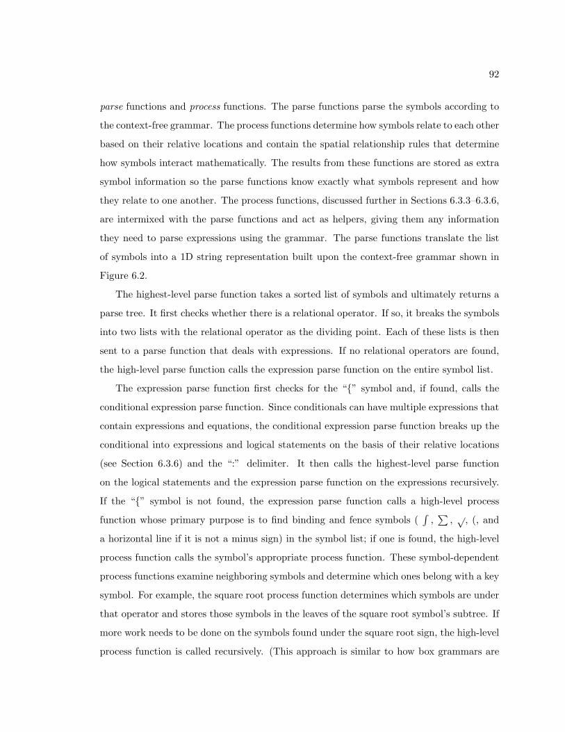
92
parse functions and process functions. The parse functions parse the symbols according to
the context-free grammar. The process functions determine how symbols relate to each other
based on their relative locations and contain the spatial relationship rules that determine
how symbols interact mathematically. The results from these functions are stored as extra
symbol information so the parse functions know exactly what symbols represent and how
they relate to one another. The process functions, discussed further in Sections 6.3.3–6.3.6,
are intermixed with the parse functions and act as helpers, giving them any information
they need to parse expressions using the grammar. The parse functions translate the list
of symbols into a 1D string representation built upon the context-free grammar shown in
Figure 6.2.
The highest-level parse function takes a sorted list of symbols and ultimately returns a
parse tree. It first checks whether there is a relational operator. If so, it breaks the symbols
into two lists with the relational operator as the dividing point. Each of these lists is then
sent to a parse function that deals with expressions. If no relational operators are found,
the high-level parse function calls the expression parse function on the entire symbol list.
The expression parse function first checks for the “{” symbol and, if found, calls the
conditional expression parse function. Since conditionals can have multiple expressions that
contain expressions and equations, the conditional expression parse function breaks up the
conditional into expressions and logical statements on the basis of their relative locations
(see Section 6.3.6) and the “:” delimiter. It then calls the highest-level parse function
on the logical statements and the expression parse function on the expressions recursively.
If the “{” symbol is not found, the expression parse function calls a high-level process
function whose primary purpose is to find binding and fence symbols (∫
,∑
,√
, (, and
a horizontal line if it is not a minus sign) in the symbol list; if one is found, the high-level
process function calls the symbol’s appropriate process function. These symbol-dependent
process functions examine neighboring symbols and determine which ones belong with a key
symbol. For example, the square root process function determines which symbols are under
that operator and stores those symbols in the leaves of the square root symbol’s subtree. If
more work needs to be done on the symbols found under the square root sign, the high-level
process function is called recursively. (This approach is similar to how box grammars are

93
<math_formula> ::= <equation> | <expression>
<equation> ::= <expression> <relational_op> <expression> |
<expression> ‘‘=’’ <cond_expression>
<relational_op> ::= ‘‘=’’ | ‘‘~=’’ | ‘‘<’’ | ‘‘>’’ | ‘‘<=’’ | ‘‘>=’’
<cond_expression> ::= ‘‘{’’ <cond_statement>
<cond_statement> ::= ‘‘if’’ <expression> ‘‘:’’ <logic_expression>
{‘‘elseif’’ <expression> ‘‘:’’ <logic_expression> }
<expression> ‘‘: else’’
<logic_expression> ::= <equation> <logical_op> <logic_expression> | <equation>
<logic_op> ::= ‘‘and’’ | ‘‘or’’
<expression> ::= <term> ‘‘+’’ <expression> |
<term> ‘‘-’’ <expression> |
<term> ‘‘^’’ <expression> |
<term>
<term> ::= <factor> ‘‘*’’ <term> |
‘‘(‘‘ <expression> ‘‘)’’ |
<factor>
<factor> ::= <sub_expression> ‘‘/’’ <factor> |
<sub_expression>
<sub_expression> ::= <integral> | <derivative> | <summation> |
<function> | <terminal>
<integral> ::= ‘‘int(‘‘ <expression> ’’,’’ <variable> ‘‘)’’ |
‘‘int(‘‘ <expression> ‘‘,’’ <variable> ‘‘,’’
<expression> ‘‘,’’ <expression> ‘‘)’’
<derivative> ::= ‘‘diff(’’ <expression> ‘‘,’’ <variable> ‘‘)’’ |
‘‘diff(‘‘ <expression> ‘‘,’’ <variable> ‘‘,’’
<integer> ‘‘)’’
<summation> ::= ‘‘sum(‘‘ <expression> ‘‘)’’ |
‘‘sum(‘‘ <expression> ‘‘,’’ <expression> ‘‘,’’
<expression> ‘‘)’’
<function> ::= <func_name> ‘‘(‘‘ <expression> ‘‘)’’
<func_name> ::= ‘‘sqrt’’ | ‘‘abs’’ | ‘‘log’’ | ‘‘exp’’ |
‘‘sin’’ | ‘‘cos’’ | ‘‘tan’’ | ‘‘asin’’ |
‘‘acos’’ | ‘‘atan’’
<terminal> ::= <variable> | <number>
<variable> ::= <letter> |
<letter> ‘‘_’’ {<integer>} {<letter>} {<integer>}
<number> ::= <integer> |
<integer> ‘‘.’’ <unsigned_int>
<integer> ::= <sign> <unsigned_int> | <unsigned_int>
<unsigned_int> ::= <digit> <unsigned_int> | <digit>
<sign> ::= ‘‘+’’ | ‘‘-’’
<digit> ::= [0-9]
<letter> ::= [a-z] | [A-Z] | [alpha-zeta]
Figure 6.2: The context-free grammar used in part to parse mathematical expressions. Notethat, for brevity, <digit> and <letter> are written using regular expression notation.

94
used, as discussed in Section 6.2.) After the high-level process function relates neighboring
symbols to key symbols based on their relative locations, the expression parse function looks
for the “+” or “-” operator and, if found, calls the term parse function on the symbols to
the left of the operator and the expression parse function on the symbols to the right of the
operator.3 However, if these operators are not found, the term parse function is called.
The term parse function looks for the explicit multiplication operator ∗ and, if found,
calls the factor parse function on the symbols to the left of the operator and the term parse
function on the symbols to the right of the operator.4 If the explicit multiplication operator
is not found, the factor parse function is called.
The factor parse function uses the information from the division process function; if a
division is found, it calls the subexpression parse function on the symbols in the numerator
and recursively calls the factor parse function on the symbols in the denominator. If a
division operator is not found, the factor parse function simply calls the subexpression
parse function.
Using the information about how neighboring symbols relate to one another, the subex-
pression parse function calls the appropriate parse function for the first symbol in its input
list. For example, if the symbol is an∫
, the integration parse function is called; if the
symbol is a function name, then the function name parse function is called. In each case,
if there is more parsing to do at the end of these symbol-dependent parse functions, the
expression parse function is recursively called to parse the remaining symbols. If the first
symbol is not a key symbol, as defined above, then the remaining symbols are sent to the
implicit operator parse function.
The implicit operator parse function first checks to see if only one symbol is in the list.
If so, it is assumed to be a terminal symbol and returned, representing a base case in the
overall parsing algorithm. If there is more than one symbol in the list, the parse function
calls a symbol direction process function that sees whether a symbol or group of symbols
are either a subscript or superscript to the first symbol or an implied multiplication with
3The grammar in Figure 6.2 shows a production for the expression nonterminal defining superscripts.This is actually an implicit operation and is parsed later in the algorithm.
4The explicit multiplication operator is rarely used in mathematical sketching since most multiplicationis expressed implicitly. However, it is important for multiplying numbers together.

95
it. Using this information, the implicit operator function calls the expression parse func-
tion on the different symbol groups, making nodes in the parse tree to reflect subscripts,
superscripts and implied multiplication. Eventually, all symbols entering the implicit oper-
ator parse function are terminal symbols and the parsing algorithm terminates, returning
a mathematical expression’s parse tree.
6.3.3 Implicit Operators
To determine if a symbol is a subscript, superscript, or to the right of another symbol
(defining an implicit multiplication), that symbol’s location needs to be examined relative to
the other’s. In general, determining implicit operators is challenging because of the variation
in symbol size and location as well as whether each symbol is an ascender, descender or
neither. Since users need to provide writing samples to train the symbol recognizer, we can
incorporate how they write ascender and descender symbols into the rules for determining
implicit operators. Users write training samples relative to predrawn boxes (see Section
5.3.1). Thus, the top and bottom of a particular symbol can be found relative to the
predrawn boxes by taking the average of the highest and lowest y coordinates of each
training sample and applying to them the transformation between the predrawn boxes and
the unit square. For example, because the letter “p” is a descender, its highest point
might be 1.0 and its lowest point might be −0.5. The highest point of an ascender like
the letter “b” might be 1.4 and its lowest point might be 0.0. With this approach, the
midpoint of a symbol is not necessarily its geometric midpoint. The midpoints of ascender
and descender letters will be slightly above and slightly below their geometric midpoints
respectively, making the implicit operator rule less rigid.
Using the ascender/descender symbol information, we can find the relationship between
two symbols s1 and s2 by first remapping the symbols to reflect the transformed average
high and low points of their training samples. For example, s1’s remapped bottom and top
y coordinates would be
botnew = − h · botbox
botbox − topbox+ topy, (6.1)

96
topnew = botnew +h
botbox − topbox(6.2)
where h is the height of the symbol in pixels, topy is the symbol’s highest y coordinate, and
botbox and topbox are the symbol’s highest and lowest y coordinates in unit square space
(assuming a coordinate system with the +x-axis to the right and the +y-axis down). Note
that botnew and topnew are still in pixel space.
If the lowest point of s2 is above the midpoint of s1, defined by (botnew+topnew)2 , then s2
is a superscript. If the highest point of s2 is below the midpoint of s1 then s2 is a subscript.
Otherwise s1 and s2 are implicitly multiplied.
6.3.4 Fractions and Square Roots
A symbol is a fraction line if it is approximately horizontal and has at least one symbol
above it and at least one symbol below it. If a fraction line is found, all the symbols in the
numerator and the denominator must be found. Given the starting and ending x coordinates
of the fraction line, vertical lines can be constructed from them that create boundaries on
which symbols should be included as part of the fraction. If a symbol falls within these
boundaries and is above the fraction line, it is in the numerator; if it is within the boundaries
and below the fraction line, it is in the denominator. This approach worked well in many
cases, but we found users tend to underestimate how long they should make the fraction
line, so that only part of a symbol is contained within the vertical boundaries, causing a
parsing error. To alleviate this problem, we took a more aggressive approach by relaxing
the vertical boundary rule. Instead requiring that a symbol must be completely contained
within the vertical boundaries, we say that a symbol is part of a fraction if any part of it is
contained within these boundaries. This relaxation adds flexibility to the fraction rule and
can correctly parse mathematical expressions like those in Figure 6.3.
As with fractions, users writing square roots often underestimate the width and height
of the symbol, and this leads to parsing errors if a strict enclosure rule is enforced. We use a
similar approach to the fraction rule. Given the square root’s bounding box, we use the four
corner points to define four separate lines, two horizontal and two vertical, that represent
the top and bottom boundaries and the left and right boundaries of the symbol. A square

97
Figure 6.3: Mathematical expressions that are parsed correctly due to the aggressiveness ofthe fraction rule. Even those symbols that are not completely within the vertical boundaryof the fraction are still included as part of the fraction’s numerator and denominator.
root is an unusual symbol in that the left and top parts of the symbol are boundaries that
users adhere to, but we still must check if a given symbol is underneath the square root
sign. A symbol is part of the square root operation if it is completely to the right of the
left boundary, below the top boundary, and if any part of it is above the bottom boundary
and to the left of the right boundary. This approach, as with fractions, gives users some
flexibility in writing square roots. Figure 6.4 show some examples.
Figure 6.4: Mathematical expressions that are parsed correctly due to the aggressivenessof the square root rule. Even those symbols that are not completely contained within thesquare root’s bounding box are still included in the square root operation.
6.3.5 Summations, Integrals, and Derivatives
Summations and integrals have similar structures in that three separate groups of symbols
may be potentially associated with them. With a summation, the lower and and upper
bounds as well as the summand are all part of the summation operation. Integrals are
similar but do not always have upper and lower limits. Summations also present difficulties
in determining where the summand ends, since there is no terminating symbol as with
integrals (i.e., the dx in∫
xdx).
We use a similar approach to parsing summations as we used with fractions and square

98
Figure 6.5: Mathematical expressions that are parsed correctly due to the aggressivenessof the summation rule. Even those symbols that are not completely contained within thesummation sign’s horizontal and vertical boundaries are included as part of the summation.
roots (see Figure 6.5). We can create four lines from the four corner points of the sum-
mation’s bounding box. All symbols underneath the summation sign and at least partially
contained within the vertical boundaries are the summation’s lower bound. All symbols
above the summation sign and at least partially contained within the vertical boundaries
are the summation’s upper bound. Note that there is no restriction on how high above or
far below the summation sign’s symbols must be for the upper and lower bounds. However,
since mathematical expressions come into the mathematical expression recognizer one at a
time, we need not worry about dealing with symbols from another expression that might fit
the lower and upper bound criteria. In addition, we assume that users write summations
in a traditional format. A summation can be the numerator or denominator in a fraction
and it is possible that other symbols in the fraction could fit the lower and upper bound
criteria. However, the parsing algorithm always deals with fractions before summations,
so this is not a problem. The top and bottom lines and the right vertical boundary from
the summation’s bounding box determine what symbols are in the summand. A symbol to
the left of the right boundary and partially contained within the top and bottom boundary
is part of the summand. To determine where the summand ends and another part of the
expression begins, users are required to enclose the summand in parentheses.
Integrals are parsed in the same way as summations except for two major differences.
First, there is more flexibility in where the lower and upper limits can be placed in relation
the the integration sign. Common notation puts these limits either directly above and
below the integration sign or slightly to its top and bottom right; we support both formats

99
Figure 6.6: Two different ways to write integration limits.
(see Figure 6.6). For limits to the top right and bottom right positions, we use the top
and bottom boundaries of the integration sign: if any symbols close to the integration
sign intersect them, they are the upper and/or lower limits. Second, because integrals are
terminated by the d <variable> symbol, we automatically know what the integrand is,
so that we do not require parentheses around the integrand. With both summations and
integrals we assume users write the summation and integral signs large enough to encompass
the summand and integrand respectively. However, they do not always do so. One way to
deal with this problem is to extend the top and bottom boundaries using the bounding box
defined by the union of the summation or integral sign and their upper and lower bounds
or limits. This approach would mean that the upper and lower bounds or limits would have
to be found before the summand or integrand. We do not currently support this feature
but we plan to incorporate it in future versions of the parsing algorithm.
For derivatives, we use fractional notation (i.e., dydx , d3y
dx3 ) instead of other more compact
notations (i.e., x, x′
) because dots and primes can be difficult to recognize robustly.5 We
parse derivatives using a combination of the implicit operator and fraction rules. The
distinguishing feature of a derivative in our notation is that it has the letter “d” in the
numerator and the denominator. Therefore, if a “d” is found in the numerator and the
denominator, the fraction is examined to see if it fits the derivative notation criterion:
that the numerator must have a “d” with an optional superscript (an integer) implicitly
multiplied by a variable and the denominator must have a “d” implicitly multiplied by a
variable with an optional superscript (another integer). If the variables are different and if
5We recognize the need for this notation and plan to allow it future versions of the parsing algorithm.

100
superscripts of the same value are present in both the numerator and the denominator, the
fraction is defined to be a derivative sign with the superscript stating that the nth derivative
should be taken. If no superscripts are found, then the first derivative should be taken.
6.3.6 Conditionals
Conditionals are used as branching instructions in mathematical sketching and are a bit
more complicated to parse than summations and integrals because multiple expressions are
involved. Figure 6.7 shows a conditional expression used in mathematical sketching. The
key to parsing conditionals is to break up the lines of mathematics so that each one can be
parsed individually and incorporated back into the conditional expression.
Figure 6.7: A conditional expression.
To parse conditionals, all unique symbol pairs to the right of the the “{” sign are
examined. If the vertical distance between a pair of symbols is greater than some threshold
(about five pixels), then the y coordinate halfway between them is a candidate breaking
location. We then extend a horizontal line through this coordinate: if no symbols intersect
the line and there are no other breaking points in the neighboring region, the candidate
becomes a breaking point. The breaking points are sorted from top to bottom and each one
is used to break the conditional expression into multiple expressions. All symbols above each
breaking point are stored in separate lists, assuming a particular symbol has not already
been placed in another list. The symbols below the last breaking point are also stored in a
list. These lists of symbols then represent the different parts of the conditional expression.
The colon in each line of mathematics is used to break up the expressions further into a
mathematical expression and a logical statement. This approach works well as long as users
put enough space between each line of mathematics in the conditional expression. In some

101
cases, however, there is enough space between lines of mathematics but a horizontal line
extended from a breaking point does not separate all the symbols in a line. What is required
in this case is to have multiple breaking points that can define polylines for separating the
mathematical expressions in a conditional expression. We currently do not support this
approach but discuss its merits in Chapter 11.
6.3.7 Reducing Parsing Decisions and Improving Symbol Recognition
With our parsing approach we can reduce the number of parsing decisions the algorithm
has to make and, using context, improve the symbol recognition accuracy. These avoidable
parsing decisions are based not on the grammar but on the spatial relationship rules. As
discussed in Section 6.1, there are many different ways of expressing mathematics and a
variety of different notations. We assume a notation that makes sense in the context of
mathematical sketching, so that some notations do not appear in our domain. Many of the
parsing decision reductions are made with implicit operators. For example, we do not allow
numbers to have subscripts. Therefore, in the implicit operator rule, if symbol a is a number
we have no need to check whether symbol b is a subscript of a. We do allow subscripts to
have multiple symbols but we do not allow subscripts or superscripts on subscripts. We also
say that only alphanumeric characters and the minus sign can be subscripts, meaning that
if symbols such as “+” and “(” are next to an alphanumeric symbol they are not part of a
subscript. The rules on superscripts are much less restrictive than those on subscripts, but
we still can reduce some of the parsing decisions the algorithm must make. As an example,
the “+” symbol can never be the first symbol in a superscript since positive numbers and
variables are implied. Operators such as “+”, “−”, and “(” also cannot have superscripts
or subscripts at all.
We can also use the parsing algorithm to assist the symbol recognizer using contextual
information. One approach [Lee and Wang 1995] uses heuristic rules to correct lexical er-
rors. For example, if 5in(x) is recognized, we assume from the similarity of 5 and “s” that
a user is trying to write a sine function, and we replace the 5 with an “s”. In another
case, if l0g(t) is recognized, the 0 is replaced with “o” since we assume the user was writing
the log function. These types of heuristics are used for all the functions our mathematical

102
expression recognizer supports. As a side effect of these heuristics, parsing decisions on the
individual symbols making up the function are eliminated.
Functions of time are commonly used in mathematical sketching (e.g., py(t)). In these
situations, the t in parentheses should never be misrecognized as a “+”. Therefore, the
parsing algorithm always looks for substrings of the form (+) and replaces the “+” with a
t. More sophisticated approaches to correcting recognition errors in context can be found
in [Chan and Yeung 2001b], and we plan to incorporate some of these in future versions of
the parsing algorithm. Chapter 10 analyzes the parsing algorithm’s accuracy and how it
adapts to different users.

Chapter 7
Mathematical Sketch Preparation
Before a mathematical sketch is made into a dynamic illustration, it must be prepared for
its translation into a simulation that ultimately animates drawing elements. The animation
requires simulation data generated from the mathematical specification (see Chapter 8) as
well as an analysis of the free-form drawings and any associated labels so as to combine
drawings and mathematics properly. In this chapter, we discuss how mathematical sketches
are analyzed so the simulation data and the free-form drawings will interact properly, using
both direct and indirect intervention from users.
7.1 Mathematical Sketch Preparation Components
Mathematical sketches need to be analyzed so that information from the free-form drawings,
any associated labels, and the data generated from the mathematics can work together
to make dynamic illustrations. This analysis is performed in real time and during a pre-
simulation step. Real-time preparation is done whenever users create a mathematical sketch.
For example, whenever users recognize a mathematical expression, the preparation system
stores that recognized expression for later use. The main type of preparation done in real
time is association inferencing. When users make an association, mathematical expressions
must be attached to a particular drawing element. With explicit associations (see Section
4.4.2), this is done by the user. However, with implicit associations (see Section 4.4.1),
the system must find the mathematical expressions to attach to a drawing element. Our
association inferencing approach is discussed in Section 7.2.
103

104
The pre-simulation step of mathematical sketch preparation, performed just before the
sketch animates, gathers important information from the sketch so it can run properly. For
a sketch to run properly, dimensional analysis, drawing rectification, and stretch determi-
nation are required. Since users are writing mathematics that will generate simulation data
and making drawings that have no information about the coordinate system used in the
simulations, the drawings and mathematics must be analyzed to determine the proper cor-
respondence between them. Drawing dimension analysis and our method for dealing with
this correspondence are discussed in Section 7.3. Another issue in mathematical sketching
is that users write precise mathematical specifications to create their dynamic illustrations
but generally make imprecise free-form drawings. To make our dynamic illustrations plau-
sible, the drawings must adhere to the mathematics. The process of correcting drawings so
they are in line with their mathematical specifications is called drawing rectification. Angle,
location, and size rectification are all critical in ensuring a plausible-looking illustration, as
discussed in Section 7.4. Finally, if nails are made to drawings, they must be analyzed to see
if nailed drawing elements should be stretched during animation or if the drawing elements
must simply be grouped together. We discuss this issue in Section 7.5.
7.2 Association Inferencing
When users make implicit associations they label drawing elements; we use these labels to
determine which written mathematical expressions to associate with a particular drawing
element. An expression should be associated with a drawing element if it takes any part
in the behavioral specification of that element. Two types of labels can be associated to
drawing elements. The first type of labels are constants (see Figure 7.1). As an example,
a user might want to associate the number 100 to a horizontal line indicating its length
and associate the constant l = 50 indicating a building’s height. With these types of
associations, inferencing is trivial: if a label is a number or equal to a number, the label
is the only mathematical expression collected and the association is complete. The second
type of labels are variable names (see Figure 7.1), which are slightly more complicated since
they generally refer to other mathematical expressions. We utilize the label families to infer
which mathematical expressions should be associated to the labeled drawing element.

105
Figure 7.1: The building and ground are labeled with constants and the stick figure islabeled with the letter “p”. Individual drawing elements and the mathematical expressionsare color-coded with a semi-transparent pastel color to show the associations.
A label family is defined by its name, a root string. Members of the label family are
variables that include that root string and a component subscript (e.g., x for its x-axis
component) or a function specification. For example, if the user labels a drawing element
φo, the inferencing system determines the label family to be φ and finds all mathematical
expressions having members of the φ label family on the left-hand side of the equal sign:
φ, φo, φ(t), φx(t), and so on. The inferencing system then finds all the variable names
appearing on the right-hand side, determines their label families, and then continues the
search. This process terminates when there are no more variable names to search for.
Consider Figure 7.1. A user labels the stick figure with a p. p represents the core label in
the label family and is used as a starting point.1 The algorithm’s first pass finds px(t) = bt
and py(t) = ct − 12gt2. It would then examine the right-hand side of these equations and
extract the symbols b, t, c, and g from them. On the second pass, the algorithm looks at
1Sometimes the core label must be extracted from a label: if the label was cx, the system would removethe subscript to yield the core label c.

106
the remaining expressions and finds b = h cos(a), c = h sin(a), t = 0 to 20, and g = 9.8.
Examining the right-hand side of these expressions yields h and a. Finally, the algorithm
examines the remaining expression and finds h = 38 and a = 0.92; since there are no more
symbols to extract, the algorithm terminates.
When the algorithm finds a related mathematical expression, it must examine that ex-
pression’s right-hand side to find other symbols that could be left-hand sides of related
expressions. Therefore, we must examine the right-hand sides, disregarding all non-symbol
information. As described in Chapter 6, handwritten mathematical expressions are trans-
lated into 1D text strings. Therefore, before we can extract symbols from the right-hand
side of an expression, we build a mask over the string that removes characters that could not
possibly be symbols, including standard functions (e.g., cos, sin, log) and operators (e.g., +,
−, ˆ, /). The mask also disregards numbers except when they follow an underscore (since
an underscore signifies a subscript). With the expression masked, symbols can easily be
extracted and tested to see if they are part of related mathematical expressions.
Once all the related mathematical expressions have been found, they are sorted to
represent a logical flow of operations that can be executed by a computational engine, and
the implicit association is completed. For example, in Figure 7.1 the system would first store
all the terminal expressions, then the expressions that are not functions of t, and finally the
time-dependent functions. Note that it is possible to have interrelated equations such as
x(t) = t2y(t) and y(t) = x(t)− t in a sketch, making sorting slightly more difficult. Future
versions of mathematical sketching will support these types of dependencies by detecting
them, solving them with Matlab (the computational engine), and enabling the user to
interactively select the appropriate solutions for their sketches.
7.3 Drawing Dimension Analysis
Mathematical sketching assumes a global Cartesian coordinate system with the +x-axis
pointing to the right and the +y-axis pointing up. However, the overall scale of the coor-
dinate system — how much screen space is equal to one coordinate unit along either axis
— must be defined. Note that individual drawing elements have their own local coordi-
nate systems with the origin at the center of the element. However, these local coordinate
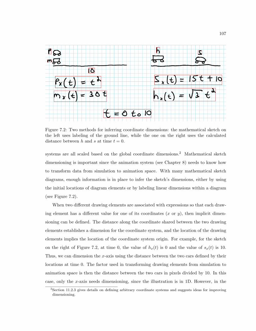
107
Figure 7.2: Two methods for inferring coordinate dimensions: the mathematical sketch onthe left uses labeling of the ground line, while the one on the right uses the calculateddistance between h and s at time t = 0.
systems are all scaled based on the global coordinate dimensions.2 Mathematical sketch
dimensioning is important since the animation system (see Chapter 8) needs to know how
to transform data from simulation to animation space. With many mathematical sketch
diagrams, enough information is in place to infer the sketch’s dimensions, either by using
the initial locations of diagram elements or by labeling linear dimensions within a diagram
(see Figure 7.2).
When two different drawing elements are associated with expressions so that each draw-
ing element has a different value for one of its coordinates (x or y), then implicit dimen-
sioning can be defined. The distance along the coordinate shared between the two drawing
elements establishes a dimension for the coordinate system, and the location of the drawing
elements implies the location of the coordinate system origin. For example, for the sketch
on the right of Figure 7.2, at time 0, the value of hx(t) is 0 and the value of sx(t) is 10.
Thus, we can dimension the x-axis using the distance between the two cars defined by their
locations at time 0. The factor used in transforming drawing elements from simulation to
animation space is then the distance between the two cars in pixels divided by 10. In this
case, only the x-axis needs dimensioning, since the illustration is in 1D. However, in the
2Section 11.2.3 gives details on defining arbitrary coordinate systems and suggests ideas for improvingdimensioning.

108
2D case, if a dimension exists only for a single axis, it is also used to dimension the other
axis since this is the best information available. In addition, if there are more than two
drawing elements with different values for one of their coordinates, then we simply infer
dimensionality from the first two.
Alternatively, if only one drawing element is associated with mathematics or if more than
one drawing element is associated with mathematics but they all have the same values at
time 0, then the dimension of the coordinate system can still be inferred if another drawing
element is associated with a numerical label. Whenever a numerical label is applied to a
drawing element, it is analyzed: if it is a horizontal or vertical line, the corresponding x-
or y-axis dimension is established; otherwise, we apply the label to the best-fit line to the
drawing element and then establish the dimensions of both coordinate axes. More formally,
given a simple drawing element, which is just an ink stroke with points p and a numerical
label len, if the element is a line (we can use the Fit Line feature described in Algorithm 5.3)
we check if it is close to horizontal or vertical and dimension either axis respectively with
len. If it is neither vertical nor horizontal, then we define a normalized vector ~v1 = pn − p1
and a vector ~v2 = (sgn(xn− x1), 0). The x-axis dimension xd is (~v1 ·~v2) · len and the y-axis
dimension yd is (sin(arccos(~v1 · ~v2))) · len. The factors for transforming drawing elements
from simulation to animation space are then the x and y distances for the drawing element
in pixels divided by the numerical label in the horizontal- and vertical-line case and xd and
yd in all other cases. For example, with the sketch on the left of Figure 7.2, at time 0 both
hx(t) and sx(t) are 0, offering no help with defining coordinate dimensions. However, the
horizontal line below it is labeled with 10. Therefore, we can dimension the x-axis with 10
and define the simulation-to-animation-space transformation factor to be the width of the
line in pixels divided by 10.
Two important issues in drawing dimension analysis must be addressed. First, more
than one drawing element may have a line label, so that there are multiple possibilities for
a x or y dimension. One approach to this issue is simply to choose the first or last drawing
element that defines an x or y dimension. This approach works but is not necessarily
ideal; we are currently looking at ways for users to choose drawing elements to use for
dimensioning. Second, if not enough information has been specified to define coordinate

109
system dimensions implicitly, then default dimensions are used. This default works for
many mathematical sketches but is sometimes insufficient, resulting in drawing elements
that hardly move at all or move quickly off the screen. One approach to this problem
is to examine the minimum and maximum values that a drawing element obtains during
simulation and use it to dimension the coordinate system so that drawings always move
appropriately. We explore the plausibility of this approach in Chapter 11.
7.4 Drawing Rectification
Mathematical sketches often have inherent discrepancies between what the mathematics
specifies and what the user draws: that is, mathematical expressions in user drawings often
do not agree precisely with their associated visual relationships. In other words, because
users write precise mathematical specifications and make imprecise free-form drawings, the
correspondence mismatch between the two often yields a dynamic illustration that looks
incorrect. Consider the pendulum in Figure 7.3. A user draws a pendulum and defines an
angle between it and the vertical. Then the user writes a = 0.5, which is used as the initial
angle in the pendulum’s motion calculations. However, the actual angle made between the
pendulum and the vertical is not 0.5, and the pendulum moves incorrectly (the theoretical
resting position would be at an angle off the vertical). Therefore when an illustration is
run, the drawing must be adjusted to match the mathematics or vice versa. To deal with
this problem we rectify drawings.
Rectification is the process of fixing the correspondence between drawings and math-
ematics so that something meaningful is displayed. Our system supports angle, location,
and size rectification, all critical in many dynamic illustrations. Rectification is a difficult
problem and converges to the general constraint satisfaction problem. One of the goals of
our rectification strategies is to see how far we can get without using a constraint solver. In
many cases, rectification in mathematical sketching is simplified since angle rectification is
designed to handle only simple acyclic relationships between drawing elements and we do
not check for cycles during this process. In other cases, rectification is more complicated
(see Section 11.2.3 for strategies for dealing with more complex rectification).

110
7.4.1 Angle Rectification
Figure 7.3: The effects of labeling an angle: a user draws the pendulum on the left andwrites a = 0.5. When an angle label is made, the drawing is rectified based on the initialvalue of a (in radians) and the pendulum on the right is rotated to reflect a. The greendot shows the rotation point (computed using Algorithm 4.4) and the magenta arrow showswhich part of the drawing will rotate during the dynamic illustration.
Mismatches between numerical descriptions of angles and their diagram counterparts are
readily discernible. When an angle such as a in Figure 7.3 is associated with mathematics,
we rectify the drawing in one of two ways. First, the angle between the two lines connected
by the angle arc is computed. Given the point of rotation pa and points on the initial and
terminal sides of the angle pi and pt, we define two normalized vectors ~v1 = (pi−pa)‖pi−pa‖ and
~v2 = (pt−pa)‖pt−pa‖ . The angle specified by the drawing is then arccos(~v1 · ~v2). Next, the system
determines if a mathematical expression corresponding to the angle label already exists. If
so, it rotates the active line about pa, as determined by the difference between the drawing
angle and numerical label, to the correct place based on the mathematical specification.
If not, it uses the angle computed from the drawing as the numerical specification of the
angle’s value. Currently, this angle is represented internally and used during simulation.
Our angle rectification strategy works well when angles are defined by two isolated
drawing elements, as in Figure 7.3. However, it fails in certain situations. For example,
an angle must be defined by two separate drawing elements. If users draw the initial and
terminal sides of an angle with one stroke (e.g, the first two sides of a triangle), the angle
rectification algorithm cannot handle it. We could deal with this issue by detecting vertices
and breaking the stroke into parts. A more difficult situation is illustrated in Figure 7.4:
an angle rectification can break a drawing. Performing angle rectification on the angle in

111
Figure 7.4: Angle rectification breaks down when additional constraints are applied. Thetop sketch shows a three-stroke triangle whose base is given a width of 200. The bottomsketch shows an angle rectification made to the top angle that breaks the triangle. Thequestion here is whether the triangle should be maintained.
Figure 7.4 breaks the triangle. Furthermore, because the base of the triangle is labeled
as 200, we now must choose between maintaining the triangle by shortening the triangle
base and the terminal side of the angle or maintaining the length of the triangle base and
readjusting the other sides of the triangle to rectify the angle. It can also happen that what
the rectification process does is sufficient (as in the bottom triangle in Figure 7.4). Thus,
the complexity of angle rectification increases as drawings become more complex and when
multiple labels are present. Two possible approaches to these problems are to employ a
constraint solver with a sophisticated suggestive user interface [Igarashi and Hughes 2001]
by which users can choose what they want to happen, or to use a simple set of rules to
deal with angle rectification. The tradeoffs and plausibility of these two approaches are
discussed in Section 11.2.3.

112
7.4.2 Location Rectification
User drawings often contain drawing elements placed in relation to other elements. If a
drawing element is placed incorrectly with respect to other drawing elements and their
mathematical specifications, the dynamic illustration does not look correct and may not
present the right visualization. Consider the sketch in Figure 7.5 (this is the same sketch
discussed in Section 1.3.3). The user draws the ball but positions it a bit to the right on
the horizontal line. However, to see whether the ball will travel over the fence (a distance
of 100 units), the ball should be placed so that it starts at distance zero, which is at the
start of the horizontal line. Since this is a 2D sketch, the ball should also be placed at a
certain height from the ground. In both cases, we want to place the ball using the initial
conditions of the mathematical specification in relation to any labeled drawing elements. In
our example, the ball should be at location (0, 3) with respect to the horizontal line, since
the initial conditions for its position are defined by px(0) and py(0) (see Figure 7.6). Now
the system must rectify the ball’s position in order to make a valid correspondence among
the ball, the labeled lines, and the mathematics.
To perform location rectification, we begin by looking at all drawing elements associated
with functions of time. Each of these elements is checked for explicitly written initial
conditions specified by mathematical expressions, found by using the drawing element’s core
label. The mathematical expressions associated to the drawing element are examined: if
they contain the core label on the left-hand side of the equal sign as a function evaluation,
such as the px(0) and py(0), the right-hand sides of these expressions are taken as the
initial condition values. If there is no core label (because an explicit association is used) or
no explicitly written initial conditions, we can still find initial conditions for the drawing
element by looking at the simulation data’s initial values. This data is calculated from
the transition of the mathematical expressions into executable code (see Chapter 8). Once
the initial conditions for a drawing element are found, the remaining drawing elements
are examined and the information from drawing dimension analysis is used to relocate the
drawing element. Drawing elements are relocated based not only on the dimensioning of
an axis, but also on the location of the drawing element from which that dimension came,
since we want to maintain the relationship between the two. Therefore, we examine each

113
Figure 7.5: A mathematical sketch created to illustrate projectile motion with air drag.If the ball labeled “p” is not positioned correctly with respect to the horizontal line, it isdifficult to verify whether the mathematics drives the ball over the fence.
drawing element not associated with a function of time to see if it has a line label and a
dimension for the x- or y-axis. If it has a dimension for the x-axis, we look at its start
and end x coordinates and choose the smallest. The smallest x coordinate is chosen since
we assume the origin along the x-axis is always defined as the leftmost x coordinate of the
drawing element. With the x coordinates for the origin ox, initial condition px0, and the
center of the drawing element dx we want to relocate, we then calculate a translation factor
tx = −(dx − ox) + px0 · sax, (7.1)
where sax is the dimensioning factor for the x-axis defined in Section 7.3. tx is then used
to translate the drawing element to its rectified location in the x direction. If the drawing
element with the associated line label has a dimension for the y-axis, we use the procedure
for x translation to translate the drawing element we want to rectify in the y direction, the
only difference being that we choose the bottommost y coordinate of the drawing element
with the line label as the origin along the y axis. Choosing the origin point in this way

114
Figure 7.6: The ball’s location is rectified before the illustration is run using the initialconditions px(0) and py(0), the horizontal line, and the vertical line.
facilitates an origin with the +x-axis pointing to the right and the +y-axis pointing up.
Algorithm 7.1 summarizes our location rectification approach.
Two important issues arise in our location rectification procedure. As discussed in Sec-
tion 7.3, it is possible that in a 2D mathematical sketch, only one drawing element has a line
label, meaning that only the x or y axis is dimensioned. Our drawing dimension procedure
handles this by simply dimensioning the other axis with the same dimensional information.
Since location rectification uses the information from drawing dimension analysis, the re-
location of a drawing element will reflect this information. The other important issue is
determining what happens when there is more than one x- or y-axis line label, resulting in
more than one x or y origin coordinate. In these cases, we assume that when users make
drawings they intend to put these elements in approximately the right place. We can thus
choose the origin point closest to the drawing element we want to relocate. However, if we
make this choice, the x and y dimensions may be taken from another drawing element or
elements with line labels. In this situation, the dimensions could be overridden, but this
could cause problems if another time-varying drawing element uses those dimensions. If
this happens, then separate x and y dimensions are needed for each time-varying drawing
element. Section 11.2.3 delves into the ramifications of such an approach.

115
Algorithm 7.1 Does location rectification on a list of time-varying drawing elements ADEusing a list of drawing elements NDE with possible dimension information.
LocationRectification(ADE ,NDE )(1) foreach DrawingElement ad ∈ ADE(2) ic← FindInitialConditions(ad)(3) pc ← CenterPoint(ad)(4) foreach DrawingElement nd ∈ NDE(5) P ← Points(nd)(6) if DimensionX(nd)(7) if X(P1) < X(Pn)(8) origin← P1
(9) else
(10) origin← Pn
(11) if X(ic) 6= ∅(12) tx = −(X(pc)−X(origin)) + X(ic) Width(nd)
DimensionX(nd)
(13) TranslateX(ad, tx)(14) if Y (ic) 6= ∅(15) goy ← false
(16) foreach DrawingElement nd2 ∈ NDE(17) if DimensionY (nd2)(18) goy ← true
(19) break
(20) if not goy
(21) ty = −(Y (pc)− Y (origin)) + Y (ic) Height(nd)DimensionY (nd)
(22) TranslateY (ad, ty)(23) if DimensionY (nd)(24) if Y (P1) < X(Yn)(25) origin← P1
(26) else
(27) origin← Pn
(28) if Y (ic) 6= ∅(29) ty = −(Y (pc)− Y (origin)) + Y (ic) Height(nd)
DimensionY (nd)
(30) TranslateY (ad, ty)(31) if X(ic) 6= ∅(32) gox ← false
(33) foreach DrawingElement nd2 ∈ NDE(34) if DimensionX(nd2)(35) gox ← true
(36) break
(37) if not gox
(38) tx = −(X(pc)−X(origin)) + X(ic) Width(nd)DimensionX(nd)
(39) TranslateX(ad, tx)

116
Figure 7.7: A mathematical sketch that showing a ball traveling in 1D, making an collisionwith a wall. If the ball (labeled “x”) is not the correct size in relation to the x dimensionand the mathematics, the illustration will not look correct since the ball will not appear tohit and bounce off the wall.
7.4.3 Size Rectification
The size of a drawing element in relation to other drawing elements or to the written
mathematics plays a role in the plausibility of many dynamic illustrations developed with
mathematical sketching. The mathematical sketch in Figure 7.7 illustrates a ball bouncing
off a wall in 1D. The mathematics associated with the ball uses the size of the ball to
determine when the ball collides with the wall and to update its velocity and location
with respect to the wall. The mathematics also precisely specifies the diameter of the ball
(xu = 1.2) and specifies how long the horizontal line below the ball should be (which is also
used for dimensioning x). Therefore, the ball’s behavior is precisely defined. However, the
user may or may not draw the ball with diameter 1.2 relative to the horizontal line. If the
ball is not drawn at the correct size, the dynamic illustration will not look correct, since the
ball either goes through the wall before changing direction or stops and changes direction
before it hits the wall. To remedy this situation, the ball must be resized according to the
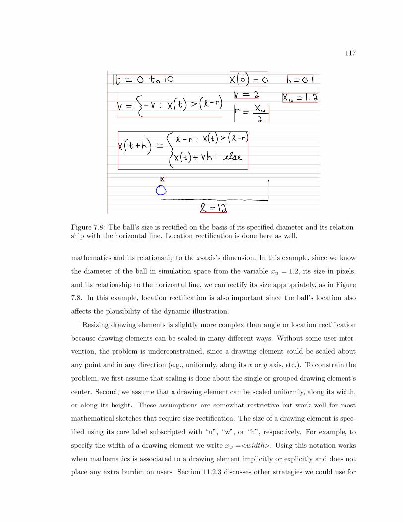
117
Figure 7.8: The ball’s size is rectified on the basis of its specified diameter and its relation-ship with the horizontal line. Location rectification is done here as well.
mathematics and its relationship to the x-axis’s dimension. In this example, since we know
the diameter of the ball in simulation space from the variable xu = 1.2, its size in pixels,
and its relationship to the horizontal line, we can rectify its size appropriately, as in Figure
7.8. In this example, location rectification is also important since the ball’s location also
affects the plausibility of the dynamic illustration.
Resizing drawing elements is slightly more complex than angle or location rectification
because drawing elements can be scaled in many different ways. Without some user inter-
vention, the problem is underconstrained, since a drawing element could be scaled about
any point and in any direction (e.g., uniformly, along its x or y axis, etc.). To constrain the
problem, we first assume that scaling is done about the single or grouped drawing element’s
center. Second, we assume that a drawing element can be scaled uniformly, along its width,
or along its height. These assumptions are somewhat restrictive but work well for most
mathematical sketches that require size rectification. The size of a drawing element is spec-
ified using its core label subscripted with “u”, “w”, or “h”, respectively. For example, to
specify the width of a drawing element we write xw =<width>. Using this notation works
when mathematics is associated to a drawing element implicitly or explicitly and does not
place any extra burden on users. Section 11.2.3 discusses other strategies we could use for

118
Algorithm 7.2 Does size rectification on time-varying drawing elements.
Input: A list of time-varying drawing elements ADE and the simulation-to-animation-space transformation factors sax and say
Output: No return valueSizeRectification(ADE ,sax,say)(1) foreach DrawingElement ad ∈ ADE(2) xfac ← 1(3) yfac ← 1(4) b1 ← BoundingBox(ad)(5) if HaveSizeWidthParam(ad)
(6) xfac ← ExtractWidthParam(ad)·sax
Width(b1)
(7) if HaveSizeHeightParam(ad)
(8) yfac ← ExtractHeightParam(ad)·say
Height(b1)
(9) if HaveSizeUniformParam(ad)
(10) xfac ← ExtractWidthParam(ad)·sax
Width(b1)
(11) yfac ← ExtractHeightParam(ad)·say
Height(b1)
(12) Translate(−CenterPoint(ad), ad)(13) ScaleAboutCenter(xfac, yfac, ad)(14) Translate(CenterPoint(ad), ad)
specifying a drawing element’s scaling information.
To perform size rectification, we first examine all time-varying drawing elements, check-
ing to see if any size information is associated to them. Size information is found by looking
at the drawing element’s core label and determining if any variable names with the core la-
bel have subscripts with “u”, “h”, or “w”. If so, the values assigned to the size variables are
extracted from the right-hand side of these equations. Using the information from drawing
dimension analysis that gives us the simulation-to-animation-space transformation factors,
we then create scaling factors for each drawing element and resize them appropriately. Note
that if no core label is present, the algorithm looks for variables starting with “u”, “w”,
or “h”, and extracts the values from those equations. Algorithm 7.2 summarizes our size
rectification procedure.
As with location rectification, the complexity of size rectification increases when more
than one drawing element has a line label, resulting in more than one choice in dimensioning
the x- and/or y-axis. We can deal with this problem, much as in location rectification, by
either updating the x- or y-axis dimensions based on which line-labeled drawing element

119
is closer to the drawing element we want to rectify or simply keeping multiple dimensions
for each axis and applying them accordingly during animation. Another important concern
with our size rectification approach is what happens when the associated mathematics lacks
size information. In these cases, it is still possible to infer scale by examining the size of the
drawing element in pixels and using the drawing dimensions to create the correct size of the
drawing element in simulation space. However, figuring out the type of size rectification
to perform (e.g., uniformly, across width or height) would be difficult without some user
intervention.
The last concern in our size rectification procedure (and with size rectification in general)
is that even with drawing element resizing, a dynamic illustration may not always look
precisely correct. The reason for these imperfections is that we let users make free-form
drawings.3 Free-form drawings have an inherent impreciseness on a geometric level that is
difficult to take into account when preparing a mathematical sketch for animation. Referring
again to Figure 7.7, we see that the mathematical specification assumes the ball is a perfect
circle. Therefore, if users draw the ball as an approximate circle, the ball can still stop
slightly before the wall or go past it by a small amount, depending on how the ball is actually
drawn. We have found that, in most cases, users don’t find these minor imperfections
significant and feel the animations are plausible, given that illustrations are based on a
sketch. Nevertheless, we discuss ways to reduce the effects of this problem in Chapter 11.
7.5 Stretch Determination
Nails allow users to pin drawing elements to the background or to one another. If a drawing
element A is nailed to another element B that is associated with time-varying mathematics,
A may have to stretch because of B’s movement. Therefore, before the dynamic illustration
can run, the mathematical sketch preparation process needs to examine these nails and
determine if any drawing element stretches during the animation.
To determine if a drawing element stretches during an animation, we examine all drawing
elements, whether or not they are associated with time-varying mathematics. For each
drawing element di, we check to see if any nails are attached to it. If so, we check to see
3Angle and location rectification suffer from this permissiveness to a lesser extent.
120
how many nails are attached to that particular element. If at least two nails are attached
to di and two of those nails are also attached to drawing elements dj , j 6= i, which has time-
varying mathematics, then we mark di as stretchable and find the two sets of spanning
points for di that are used to stretch the drawing element during animation. The spanning
points are found in two ways. First, if di is nailed to dj and dj is not time-varying, then one
set of spanning points is constant and is just the nail point. If dj is time-varying, then we
use its animation data to generate a set of spanning points. In this case, each span point spi
is defined by the animation point api plus an offset that is the original nail point subtracted
from api.4 Note that for stretch determination, we need the simulation data generated from
the mathematical specification. This data is calculated when the specification is turned
into executable code and run in the computational engine (see Chapter 8 for details). With
our approach, it is possible for a drawing element to be stretched in one or two different
directions; in addition, a single drawing element can have multiple stretchable drawing
elements attached to it. Once a drawing element is marked as stretchable, it becomes time-
varying, meaning that another drawing element attached to it could also become stretchable
and so on, creating a network of stretchable objects all stemming from one drawing element
with mathematics associated to it. Mathematical sketching does not support stretchable
object networks but they are part of our future work.
4There are different ways to calculate the spanning points depending on whether drawing elements areanimated in absolute or relative terms. If in absolute terms, the center of the drawing element is alsoneeded for the calculation.
Chapter 8
Mathematical Sketch Translation
and Animation
Transforming a mathematical sketch into a dynamic illustration hinges upon converting the
handwritten mathematics into a program. This program is then run, generating data the
animation engine uses, along with the mathematical sketch preparation data (see Chapter
7), to animate drawing elements on the screen. In this chapter, we describe how mathe-
matical specifications are translated into executable code and discuss how the animation
engine animates the drawing elements in a dynamic illustration.
8.1 Translating Mathematical Sketches into Executable Code
The mathematical specifications that users write as part of mathematical sketches are es-
sentially small programs that must be translated into the proper format to be executed in a
computational engine. The data these programs generate, along with information from the
sketch preparation routines, allow the animation engine to animate drawing elements and
create a dynamic illustration. However, we want users writing mathematical specifications
to perceive them not as a program that requires an ordered list of instructions, but rather as
a collection of mathematical statements that they might write in their notebooks to solve a
problem. This collection of mathematical statements should be order-independent from the
user’s perspective and not have the rigid structure required by conventional programming
languages.
121

122
To facilitate a more notational style, the mathematical specifications used in mathemati-
cal sketching do not require variable declarations: users simply write variables and constants
without any regard to whether they are integers or reals. The mathematical specifications
also need not be written linearly: users can write their specifications anywhere on the page,
as they might in a notebook.
However, mathematical specifications lacking structure or rules would be very difficult
to translate reliably into executable code. We therefore need some restrictions on mak-
ing mathematical specifications. First, the dynamic illustrations made with mathematical
sketching are all based on functions of time. Therefore, to animate a drawing element, the
mathematical specification associated with it must contain a function of t (e.g., px(t), y(t),
pα(t)). In addition, the function names users write must designate whether the function
should move the drawing element along the x- or y-axis or rotate it. If an “x” or “y” appears
in any part of a function name, we know to translate the associated drawing element along
that particular axis. If the function name has neither an “x” or a “y”, we know the drawing
element needs to be rotated. Second, we require a construct that lets users define and tell
the mathematical specification translator how long a dynamic illustration should run. A
traditional iteration mechanism (e.g., for loop, while loop) is such a construct, but we do
not want users to have to write them in a conventional way. In mathematics, we often see
the notation t = Tinitial ... Tfinal or t = Tinitial to Tfinal specifying the domain of a function.
This notation can effectively be used as an iteration construct as well and is a much more
“sketch-like” approach to defining iteration. Therefore, users’ mathematical specifications
must include this iteration construct as part of the specification for any moving drawing
elements in the dynamic illustration (except for stretchable objects, since their movement
is inferred from other mathematically specified drawing elements).
Mathematical sketching supports two different ways to specify the mathematics generat-
ing animation data for drawing elements. The first approach is called closed-form solutions.
With closed-form solutions, the movement of a drawing element can be defined with func-
tions whose output is known for any point in time. Thus, a closed-form function of time
can be evaluated for any time t and the result easily returned. Unfortunately, not all types
of mathematical and physical phenomena can be modeled with closed-form solutions. To

123
make mathematical sketching more expressive, we also let users employ open-form solu-
tions, in which the movement of a drawing element is not known in advance and needs
to be simulated using a numerical technique. Thus, the movement data for a particular
drawing element is determined incrementally. These two approaches are described here.
The computational and symbol engine used in mathematical sketching is Matlab, and
hence the mathematical specification translator is specifically designed to take advantage
of Matlab features and use Matlab syntax. We chose Matlab because of its computational
power and ease of use, but any computational engine could be used.
8.1.1 Closed-Form Solutions
When users invoke a mathematical sketch as a closed-form solution, two major steps are
performed on the mathematical specifications associated with drawing elements before any
data is sent to the animation engine. The first is a preprocessing step and the second is a
computation step.
The preprocessing step has two major functions. The first is to get all mathematical
expressions into Matlab-compatible format and the second is to determine which drawing
elements are animatable. Drawing elements that have functions of time and an iteration
construct are considered animatable. For each drawing element with associated mathemat-
ics, each mathematical expression is examined. If an iteration construct is found, important
information is extracted from it for later use in the computation step. This information
includes the Tinitial and Tfinal time values and optionally a discretization constant. The
drawing element containing the iteration construct is flagged as animatable as well.
Iteration constructs have different formats. Figure 8.1 shows some examples. At a
minimum, users must specify the iteration variable and the Tinitial and Tfinal time values
using either the keyword “to” or three consecutive dots. An optional part of the iteration
construct is the “by” keyword, which lets users specify the constant used to discretize the
animation time domain defined from Tinitial to Tfinal. If the “by” keyword is not used, a
default discretization constant of 0.1 is used.
If a mathematical expression is not an iteration construct, it is converted and stored as
a Matlab-compatible string. Converting mathematical expressions into Matlab-compatible

124
Figure 8.1: Different formats for the iteration construct.
strings involves two distinct steps. The first step is to remove unwanted parentheses, known
as flattening. In Matlab notation, parentheses are used to index into variables and are also
used in function calls. In the closed-form case, we need only replace parentheses in certain
situations, including multisymbol subscripts and nonstandard functions, with the “ ” sym-
bol. If these parentheses are not removed, Matlab will interpret them incorrectly, causing a
syntax error. Consider the mathematical expression py(t) = bx1sin(t). The mathematical
expression recognizer returns this expression as the 1D string p_y(t)=b_(x1)sin(t); the
flattening routine translates this string into p_y_t_=b_x1_sin(t). The key issue in this
translation is to ensure that we do not inadvertently replace parentheses we need (e.g., those
that are part of the sin function above). To avoid this, only functions that are user-defined
and multisymbol subscripts are flattened. The second step in converting mathematical ex-
pressions to Matlab-compatible strings is to introduce the “*” symbol when appropriate:
since Matlab syntax cannot handle implicit multiplication, we must introduce explicit mul-
tiplication signs as needed. These explicit multiplication operators could have been put
into the output of the mathematical expression recognizer, but resulting expressions would
look somewhat messy when displayed to users; also, we wanted the returned expressions
to be somewhat generic and not computational-engine-dependent. Explicit multiplication
signs are inserted between symbols in certain circumstances. The “*” symbol is always put
between a number and a letter except in multisymbol subscripts. In addition, “*” is always
placed in between a “)” and a letter or number or “(” as well as between letters if they are

125
not part of function names. As an example, the expression y = ( 2x1−x)2 cos(x)ex would be
transformed into y=((2x)/(1-x))^2cos(x)e^x by the mathematical expression recognizer
and converted into a Matlab-compatible string as y=((2*x)/(1-x))^2*cos(x)*e^x.
Once all the mathematical expressions are converted into Matlab-compatible strings,
the computation step is performed. In this step, the Matlab-compatible strings are used
to generate small programs that are executed using the Matlab computational engine. All
the Matlab-compatible strings for each drawing element are examined. Labels are extracted
from expressions that are functions of time so the computation routine knows if translational
and/or rotational movement is needed as part of a dynamic illustration. Next, the time
domain is discretized using the information collected from the preprocessing step, yielding
an array of time values from Tinitial to Tfinal that is sent to Matlab. Matlab is designed to
do quick computations on matrices and vectors and can vectorize mathematical expressions
so they act on an array of numbers and output an array of numbers in a single operation.
This vectorization is more efficient than computing values using a for loop. Since closed-
form solutions have the property that we can determine the value of the mathematical
specifications at any point in time, using vectorization is appropriate. Therefore, for each
type of time-varying function (i.e., x or y axis or rotation), a vectorize call is made on the
extracted labels and the vectorized function is evaluated. The evaluation step then produces
an array of values that represent the output of the function based on the discretized time
values. This array can be extracted from Matlab and stored for animation.
As an example of this process and the code generated from it, consider the mathematical
sketch in Figure 8.2. Here the user wants to see if the football will make it over the goalpost.
The mathematical specification to the left of the drawing is associated with the football.
When the user runs the sketch, the preprocessing and computation routines generate the
code (Figure 8.3) that is executed in Matlab. Once the Matlab code is run, the data from
variables xxx, yyy, and rrr are extracted from Matlab and used as input to the animation
engine.

126
Figure 8.2: A mathematical sketch: does the football go over the goalpost?
h = 38
a = 0.92
g = 9.8
b = h*cos(a)
c = h*sin(a)
p_x_t_ = b*t
p_y_t_ = c*t - (1/2)*g*t^2
p_r_t_ = 2*t
xx = vectorize(p_x_t_)
yy = vectorize(p_y_t_)
rr = vectorize(p_r_t_)
xxx = eval(xx)
yyy = eval(yy)
rrr = eval(rr)
Figure 8.3: The code generated from the mathematical specification in Figure 8.2. Notethat the variable t is an array of time values already placed into Matlab.
8.1.2 Open-Form Solutions
Open-form solutions are slightly more complicated to translate into executable code than
closed-form solutions. Before any processing can be done on an open-form solution, it must

127
Figure 8.4: A mathematical sketch with an open-form solution.
first be recognized as one. Open-form solutions can be written in many different ways (e.g.,
using subscripts or index variables). We chose a notation that was not too different from
how closed-form solutions are specified. Since the essence of an open-form solution is that
a function’s current value is determined, in part, from its previous values, users need a way
to specify this in the notation. Thus, the left-hand sides of expressions that fit this criteria
have as input parameter t+ < variable > where the “variable” is a time increment: for
example, px(t + h) = px(t) + a2. The mathematical expressions associated with a given
drawing element are examined; if any of them have t+ <variable> on the left-hand side
of the equal sign and the time increments (i.e., the symbol to the right of the “t+”) are all
the same variable, we assume an open-form solution.
Like closed-form solutions, open-form solutions have a preprocessing and computation
step. Consider the mathematical sketch in Figure 8.4. In the preprocessing step, user-
defined function names and their parameters are extracted from the mathematical expres-
sions associated to drawing elements. We need to know these names to translate the ex-
pressions to Matlab-compatible strings and to convert them into proper functions with

128
appropriate indexing. In Figure 8.4, a total of six function names and their parameters are
extracted, including the initial conditions px0(0) and vx(0) and px0(t + h), px0(t), vx(t + h),
and vx(t). Once the function names and parameters are extracted, the preprocessing step
proceeds similarly to that for closed-form solutions, looking for iteration constructs, ex-
tracting information from them used in the computation step, and converting mathematical
expressions to Matlab-compatible strings. In converting expressions to Matlab-compatible
strings, the function names and parameters are passed to the conversion routine to ensure
correct placement of explicit multiplication operators, and the user-defined function names
are treated as variable names. In addition to this conversion routine, a replacement opera-
tion is performed: all substrings of the form (t+ <variable>) and (t) are replaced with (i)
and (i− 1) respectively. This step is needed so i can be used as an index into the variables
that become arrays of numbers. In our example, px0(t + h) is translated to p__x0_(i),
px0(t) is translated to p__x0_(i-1), and so on. The last part of the preprocessing routine
deals with the initial conditions. In Matlab, array indices start with one instead of zero as
in C or C++, so all initial conditions must be converted appropriately. If a user-defined
function has a number as a parameter, we assume it is an initial condition and set it to one.
This operation also has the side effect of populating the first elements of the arrays used in
the computation step.
h = 0.1
p__x0_(1) = 0
v_x(1) = 0
a__x1_ = 3
for i = 2:100
v_x(i) = v_x(i-1) + a__x1_*h;
p__x0_(i) = p__x0_(i-1) + v_x(i);
end
Figure 8.5: Code generated from the mathematical specification in Figure 8.4.
For each animatable drawing element, the computation step first breaks the Matlab-
compatible strings into two lists based on whether or not the strings contain the index
i. We do this in order to sort the strings containing the index i so they can be properly
placed within an iteration construct. Using the time increment variable found when the

129
Figure 8.6: A mathematical sketch with an open-form solution that has conditionals.
mathematical sketch was examined to see if it was an open-form solution, the number of
iterations is calculated using⌈
(Tfinal−Tinitial)∆t
⌉
, where ∆t is the time increment variable.
With this information the Matlab code is constructed and executed and the data is stored
in arrays named after the user-defined functions in the mathematical specification. The
code generated for our example is shown in Figure 8.5.
As another example, consider Figure 8.6, a more complicated mathematical sketch using
conditionals. The code generated from this mathematical specification appears in Figure
8.7. The last step in the computation procedure for open-form solutions is determining
where to store the data generated from the executed code. One of the problems with open-
form solutions is that very often the mathematical specifications must compute velocity
and acceleration as functions of time in the x or y directions in addition to rotation. With
implicit associations, the core label is simply used to guide extracting the data from Matlab
and storing it in the appropriate arrays. However, when users make an explicit association
it may well be difficult to know which functions of time should be used to translate and/or
rotate a drawing element. In general, most open-form solutions have more mathematics

130
h = 0.1
x_u = 1.6
v = 2
r = x_u/2
l = 12
x(1) = 5
for i = 2:200
if (x(i-1) < r | x(i-1) > (l-r))
v = -v;
end
if (x(i-1) > (l-r))
x(i) = l-r;
elseif (x(i-1) < r)
x(i) = r;
else
x(i) = x(i-1) + v*h;
end
end
Figure 8.7: Code generated from the mathematical specification in Figure 8.6.
than closed-form solutions, so users would tend to use implicit associations, but an explicit
association could be used in some cases. There are two possible approaches to dealing
with the explicit association problem. The first is to constrain users to naming translation
functions only with x or y with no subscripts. Rotation functions could be named with r
or a Greek letter such as α or θ. This naming convention ensures the data generated in
Matlab is extracted and stored in the appropriate arrays, but limits users in making their
mathematical sketches. The second approach is to let users make an explicit association
merely by drawing a line through the main mathematical expressions that specify how draw-
ing elements are animated. The association inferencing mechanism would then infer which
auxiliary mathematical expressions should be part of the association. The mathematical
expressions with lines drawn through them would be used to determine how to extract
and store the Matlab data. This second approach is not currently part of mathematical
sketching but will be included in future versions.

131
8.2 The Animation System
The animation system’s sole purpose is to move drawing elements around the screen on the
basis of the data generated from their mathematical specifications. Before the animation
data is sent to the animation engine, it is first transformed into animation space using the
transformations defined from the mathematical sketching preparation routines discussed in
Chapter 7. The transformed data and the required drawing elements, including those found
in stretch determination, are then sent as input to the animation engine.
Two important design decisions were needed for the animation engine. The first was
whether to perform the animation in absolute or relative terms. We chose an absolute
approach since the data used to drive the animations was constructed in absolute terms.
The second design decision was how to define the tick value for the animation function.
This value needs to be defined so that the animation looks appropriate. We initially chose a
constant tick value, and this worked well for most cases. However, with the ability to change
the discretization constant, a constant tick value did not work as well. In many cases, a
fine discretization would mean that more data was used in the animation, making it appear
slower during a dynamic illustration. To alleviate this, we made the animation tick value a
variable defined as a function of the discretization constant, so that the animations appear
at the same speed in all but extreme cases. Having the animations appear at the same
speed has disadvantages: users might want to see a dynamic illustration in slow motion so
as to observe subtle details in a drawing element’s motion, or they might want to see a long
animation very quickly. We currently do not support this level of control, but plan to do
so in a future version of mathematical sketching (see Chapter 11).
The animation engine calls a tick function for each element in the animation data arrays;
we assume the lengths of these arrays are identical. For every tick function call, each
animatable drawing element is translated by its current x and/or y position data subtracted
from the drawing element’s original x and/or y location. If rotation is required, the drawing
element is rotated about a rotation point defined by the association by its current rotation
angle subtracted from the drawing element’s initial angle. In addition, stretchable drawing
elements are stretched on the basis of the movement of the drawing elements they are
attached to. The stretch operation uses the nail and spanning points, described in Chapter

132
Algorithm 8.1 Stretches a drawing element.
Input: A drawing element de, nail points nail1 and nail2, and span pointsspan1, and span2.Output: The stretched drawing element.StretchDrawingElement(de,nail1,nail2,span1,span2)(1) vold ← V ector(X(nail1)−X(nail2), Y (nail1)− Y (nail2))(2) vnew ← V ector(X(span1)−X(span2), Y (span1)− Y (span2))(3) αold ← acos(Y ( vold
‖vold‖) · Sign(X(vold)))
(4) αnew ← acos(Y ( vnew
‖vnew‖) · Sign(X(vnew)))
(5) Translate(−nail2, de)(6) RotateAboutOrigin(αold, de)
(7) ScaleAboutCenter(1.0, ‖vnew‖‖vold‖ , de)
(8) RotateAboutOrigin(αnew, de)(9) Translate(span2, de)(10) return de
7, to stretch a drawing element. Algorithm 8.1 summarizes the stretching routine. Once
control is returned from the animation engine, users can easily rerun the animation or
modify their mathematical sketches.
Chapter 9
MathPad2
The MathPad2 application prototype was developed to put mathematical sketching into
practice. This chapter examines MathPad2 ’s functionality and software architecture.
9.1 Functionality Summary
In order to explore the feasibility of mathematical sketching, an implementation was re-
quired to test ideas and obtain user feedback. MathPad2 , an embodiment of the mathe-
matical sketching paradigm, is this implementation. Mathematical sketching is a novel and
broad interaction paradigm, and MathPad2 implements only some of the many possible
features that the idea of mathematical sketching affords. This feature subset has been de-
scribed in Chapters 4 – 8 and other ideas that have not been implemented are described in
Chapter 11. In this section, we summarize MathPad2 ’s functionality.
The MathPad2 application is the result of a series of rapid prototyping exercises, each
one providing insight for improving mathematical sketching. These prototypes and the
lessons learned developing them are discussed in Appendix A. The current MathPad2 pro-
totype supports many types of mathematical sketches and a set of supporting computational
and symbolic tools. Since the application is a prototype, MathPad2 can operate on many
but not all mathematical expressions.
The supporting tools let users graph mathematical expressions written as functions.
More than one function can be graphed at once by overlaying them on a graph widget.
The graph widget also has a “hold plot” option so that previously plotted functions are
133

134
not erased. MathPad2 assumes Cartesian coordinates and can graph only functions of x
or t. The function names (i.e, left-hand sides) are unrestricted and need not include input
parameters. Once functions are plotted in the graph widget, their domains or ranges can
be modified by writing in new values. MathPad2 can graph a variety of different functions
but does not handle discontinuous functions or those with parts of their ranges undefined.
The supporting tools also let users solve simple equations, simultaneous equations, and
ordinary differential equations. Users can solve up to four simultaneous equations with
four unknowns. For ordinary differential equations, it is optional for users to specify initial
conditions, and the types of ordinary differential equations that can be solved are based
on the solving capabilities of the computational engine (i.e., Matlab). MathPad2 lets users
evaluate mathematical expressions. Integrals and summations can be evaluated numerically
and symbolically, as can double, triple, etc. integrals and sums. Mathematical expression
differentiation is supported to the nth order but is limited to functions of x and t. Users can
simplify, expand, and factor single mathematical expressions or groups of them. MathPad2
also lets users call a variety of standard functions including sine, cosine, tangent, arcsine,
arccosine, arctangent, logarithm (log), absolute value (abs), and the exponential (exp or e).
The functionality of all the supporting tools is restricted by the capabilities of Matlab, as is
how the mathematical expressions are specified. Future versions of MathPad2 will reduce
these restrictions.
MathPad2 has many different constructs for creating mathematical sketches. To make
drawings, users can create simple drawings or make more complex multistroke drawings by
grouping them together to form composite drawing elements. Users can also nail drawing
elements to one another or to the background, and these nails can make drawing elements
stretch depending on the motion of other drawing elements. MathPad2 lets users create
closed-form and open-form mathematical specifications to driving the animation of drawing
elements. With both forms, drawing elements can be translated in the x or y dimension
and rotated about a given point. Both forms support iteration, so animation times can be
defined, and conditional constructs, so users can specify discontinuous functions. However,
nested iteration and nested conditionals are not supported in MathPad2 . The closed-form

135
approach lets users specify drawing element motion with simple functions, while the open-
form approach lets users write simple numerical schemes to specify drawing element motion.
The number of moving drawing elements in MathPad2 is theoretically unlimited. Iteration
in combination with the conditional constructs lets users specify collision behavior between
drawing elements as well.
MathPad2 lets users make either implicit or explicit associations of mathematics to
drawings. Implicit associations let users attach variable names to drawing elements; the
variable is used to infer which mathematical expressions to attach to that element. Explicit
associations let users draw a line through the mathematics and then tap on a drawing
element to make an association. Once mathematical sketches are made, MathPad2 lets
users easily change constant values and mathematical expressions to observe how they
affect drawing element motion.
In addition to these features, MathPad2 can save and load recognized mathematical
expressions. It also lets users choose between looseleaf and graph-paper backgrounds. As-
sociations can be visualized using semi-transparent pastel colors and the bounding boxes of
graphed functions can be colored to reflect their plot lines.
9.2 Software Architecture
The MathPad2 application prototype was developed on a Tablet PC using C# and the
Microsoft Tablet PC SDK. This SDK provides a number of useful features for dealing
with and maintaining ink strokes: nearest-point and stroke-enclosure tests, transformation
routines, and bounding-box functions. As a computational and symbolic back end, we use
Matlab via its API for communicating with the Matlab engine from external programs.
The software has the distinct components shown in Figure 9.1. The main software
component is the user interface, which is the major link to other parts of the MathPad2
system. The user interface component contains the data entry objects for dealing with
inking and storage of ink strokes and recognized mathematical expressions. As users make
ink strokes on the screen, the gesture analyzer continuously examines them to determine
whether they are gestural commands or simply digital ink. If the ink strokes are commands,
then the gestural analyzer communicates with other components so that the appropriate

136
Data EntryGestureAnalyzer
CorrectionUI
User Interface
SymbolClassification
ExpressionParsing
MathematicalExpressionRecoginzer
AssociationInferencing
DimensionAnalysis
Sketch
Rectification
Sketch PreparationMathematical
Open Form
Solver
SolverClosed Form
Matlab CodeGeneration
MatlabEngine
and OuputAnimation System
Symbolic andComputation
Toolset
Figure 9.1: A diagram of MathPad2 ’s software architecture.
actions are performed. The last part of the user interface component is the correction
user interface, which lets users make corrections to incorrectly recognized mathematical
expressions on a symbol level and on a parsing level.
When users make a mathematical expression recognition gesture (i.e, lasso and tap), the
gestural analyzer sends the ink strokes to the mathematical expression recognizer, which
contains the mathematical symbol recognizer and the expression parsing system. The math-
ematical symbol recognizer is in charge of taking a collection of ink strokes, segmenting them
into symbols, and classifying the symbols as particular characters. The expression parser
takes the collection of recognized symbols and does a structural analysis pass on them to
create mathematical expressions that are sent back to the user interface component.
When users issue a command for a computational or symbolic function, the user interface
component sends the appropriate recognized mathematical expressions to the computational
and symbolic toolset. This component converts the recognized expressions into a command
that is then sent to Matlab for processing. The Matlab engine processes the command and
sends the data back to the computational and symbolic toolset, which then sends the results

137
to the animation and output component for display.
When mathematical sketches are created, the user interface component sends ink strokes
to the mathematical expression recognizer for processing and, using those results and as-
sociated drawing elements, creates a behavior list that is sent to the sketch preparation
component. The user interface component also communicates with the association infer-
encing part of the sketch preparation component in real time whenever implicit associations
are made. The sketch preparation component does drawing dimension analysis and drawing
rectification, using the data in the behavior list, and also sends the list to the Matlab code
generation component. The Matlab code generation component is in charge of using the
mathematical specification as well as information from the sketch preparation component
to generate Matlab executable code that is sent to the Matlab engine. Once the Matlab
engine executes the mathematical sketch code, the data is extracted and sent to the anima-
tion system where the animation engine moves any animatable drawing elements based on
their mathematical specifications.
Chapter 10
Recognizer Accuracy and
MathPad2 Usability Experiments
To examine how users interact with mathematical sketching and the MathPad2 application,
we ran two interrelated user studies. Because mathematical expression recognition is so
critical in mathematical sketching, our first study examines our recognizer’s accuracy on
several levels, including symbol and parsing recognition. Using subjects from the first study,
our second study evaluates MathPad2 ’s usability. In this chapter, we describe these studies
and present their results.
10.1 User Evaluation Goals
The major focus of our user studies was to evaluate the usability of mathematical sketch-
ing in the context of the MathPad2 application. More specifically, these studies examine
MathPad2 ’s ease of use, gesture learnability and which MathPad2 features subjects like the
best and the least and why. We are interested in how easy it is for subjects to pick up and
use MathPad2 with minimal training and in how many mistakes they make in performing
various MathPad2 tasks. Because MathPad2 ’s modeless gestural user interface is not nec-
essarily designed for the novice user, we are also interested in how well subjects remember
various gestural commands, since this indicates how easy they are to learn and recall. Ad-
ditionally, we are interested in whether subjects would use mathematical sketching in their
work and in what other features they would like to see added to the MathPad2 application.
138
139
Since recognizing mathematical expressions is such a critical component of mathemat-
ical sketching, it is important to have a good understanding how how well the recognizer
performs. Since the recognizer is really two interdependent parts (mathematical symbol
recognition and mathematical expression parsing), we need to examine the accuracy of both
pieces and how they affect each other. To evaluate symbol recognition, we examine the cur-
rent mathematical symbol recognizer’s performance against our previous writer-dependent
approach. In addition, we examine how well our parsing system converts the mathematical
symbols into coherent expressions. Another reason for evaluating our mathematical expres-
sion recognizer is to determine how subjects’ performance with it ultimately affects their
performance with MathPad2 .
10.2 Mathematical Symbol and Expression Recognition
Study
The first part of gauging MathPad2 ’s overall usability is to determine how well our mathe-
matical expression recognizer performs on users’ handwritings. In addition, we want to see
how well our current recognizer does against our previous writer-dependent approach.
10.2.1 Experimental Design and Tasks
Before subjects can participate in the recognition tasks, they all must provide writing sam-
ples to train the mathematical symbol recognition portion of the mathematical expression
recognizer. Each subject is introduced to the training application (described in Section 5.3):
the subject is shown the training interface, how to write on the screen, how to erase ink
(using the scribble erase gesture), and how to store writing samples in the system. Subjects
then write each symbol 20 times. The first 10 are written normally and the second 10 are
written as small as possible, for reasons discussed in Section 5.3.1. Subjects are instructed
to scribble out and rewrite symbols they are not happy with before committing them to the
system. Subjects provide writing samples for 48 different symbols including a − z, 0 − 9,
Σ, (, ), -,√
,∫
, {, <, >, +, 6=, and else.1 We chose this particular symbol set because
1The “.” and “:” symbols are also part of the symbol set but subjects need not provide samples for them.

140
it is the minimal set needed to create mathematical sketches or use tools that MathPad2
supports. The mathematical symbol recognizer supports uppercase letters and some Greek
letters, but we did not feel it necessary to include these characters in this experiment.
To guide subjects in symbol training, they were given a symbol sheet showing a hand-
written version of each symbol. The purpose of this sheet is twofold. First, the sheet shows
how each symbol needs to be written in the context of the training application’s symbol
boxes. As discussed in Section 5.3.1, the training application stores not only the ink strokes
but also the symbol’s relationship to the symbol boxes. These symbol boxes let the training
application determine whether symbols are ascenders or descenders, information later used
in the mathematical expression parsing algorithm. Second, the sheet shows how certain
symbols should be written. While, in general, subjects can write symbols however they
want, it is very difficult to distinguish among certain characters (see Figure 5.1). There-
fore, we ask subjects to provide writing samples for symbols such as “1”, “l”, “t”, and
“+” exactly as they are written on the symbol sheet. The recognizer then trains on these
samples and subjects are instructed to write each symbol once on the recognition panel in
the training application to ensure there are no problems. If the recognizer has difficulty
with a particular symbol, subjects reenter the samples for that symbol and the recognizer
retrains on the data. Note that subjects were encouraged to put down the stylus after 15
to 20 symbols so their hands would not tire. It took subjects an average of 50 minutes to
enter their writing samples.
After the training phase, subjects are run through the mathematical symbol accuracy
test. Subjects were instructed to write each symbol 12 times when prompted by the training
application, then click on a button to commit their test data. Subjects wrote test samples
for each symbol in the order in which they were trained. Subjects were also instructed
to erase and rewrite any symbols they were not happy with. We ask subjects to perform
this task for several reasons. First, we want to evaluate how our current symbol recognizer
performs when subjects focus solely on the mathematical symbols they are writing rather
than on the mathematical expressions. Second, we wanted a normalized test so that each
symbol would have equal weight in determining the recognizer’s accuracy. Third, we wanted
to evaluate the recognizer’s accuracy without constraining subjects to write symbols, with

141
widely varying sizes, as occurs frequently when writing mathematical expressions (e.g., sub-
scripts, integration limits). Finally, from our observations of how people write, we wanted
to look for any significant differences between the symbol recognizer’s performance when
subjects are writing a symbol repeatedly versus writing them in mathematical expressions.
Ideally, a recognizer should be robust in both cases with no significant differences. Subjects
were encouraged to take short breaks after every 10–15 symbols. On average, subjects took
about 25 minutes to complete this test.
After a short break, subjects were run through the mathematical expression accuracy
test. Before taking the test, subjects are asked to write a few simple trial expressions such
as x2, x1,35 ,√
xyz, and∫ 20 xdx. These expressions give subjects a feel for the recognizer and
an idea of how it parses mathematical expressions. Note that we purposely kept subjects’
practice time to a minimum to reduce any adaptation they might make to the recognizer.
Since we designed the parsing rules (Chapter 6) to be general, it is important to evaluate
how well subjects’ written expressions fit within those rules.
Subjects write 36 different mathematical expressions, writing each one when prompted
by the training application. Subjects recognize the expression by clicking on a button
and then click on another button to commit their data. Subjects were told to write each
expression neatly, as if writing a homework assignment to hand in to a professor. As in the
mathematical symbol accuracy test, subjects were asked to erase and rewrite any symbols
they were not happy with before recognizing the expression. The mathematical expressions,
chosen from a set used in Chan’s recognition experiments [Chan and Yeung 1998b] plus
expressions of our own design, are listed in Appendix C. The test expressions range from
simple to complex and are representative of the types of expressions users would write
in MathPad2 . Other more complex expressions were chosen specifically for testing the
mathematical expression recognizer. (Of course, these more complex expressions could be
used in MathPad2 as well.) Subjects were encouraged to take breaks after writing 10–15
expressions so their hands would not tire. On average, subjects took about 45 minutes to
complete this test.

142
10.2.2 Participants
Eleven subjects (seven male and four female) participated in the mathematical symbol and
expression recognizer accuracy study. Their ages ranged from 19 to 38, and all were students
or staff of Brown University. Subjects included computer science students and research staff
members as well as physics and applied mathematics majors. Only one subject was left-
handed. Six subjects had never used a Tablet PC before, while one had used a PDA
and the other four had used Tablet PCs extensively. Of the 11 subjects, two of them
were considered experts in using our mathematical expression recognizers, two of them had
used our recognizers only in passing, and the remaining seven subjects had never used the
recognizers.2 We wanted to have two subjects with expert knowledge of our recognizers to
provide a benchmark for how well users could perform with extensive training and use of
our recognition engines. All subjects were paid $30 for their time and effort.
10.2.3 Evaluation Measures
In general, determining the accuracy of a mathematical expression recognizer is a chal-
lenging problem [Blostein and Grbavec 1997]. Evaluating the symbol recognition portion
of a expression recognizer is straightforward — one just counts the number of correctly
recognized symbols. However, evaluating the parsing part of a mathematical expression
recognizer is much more challenging because of the many different errors that can occur —
lexical, syntactic, semantic, and logical. For example, parsing systems depend on the accu-
racy of the symbol recognizer. One possible solution is always to give the parsing algorithm
mathematical symbols that are 100% correct [Anderson 1968, Grbavec and Blostein 1995,
Twaakyodo and Okamoto 1995]. However, doing so does not provide an overall evalua-
tion of the mathematical expression recognizer. In our case, it is important to see how
well the parsing step performs with mathematical symbols that may not always be cor-
rect, since this is what happens in practice. Another difficulty in evaluating the parsing
step of a mathematical expression recognizer is defining the evaluation metric. One ap-
proach is to divide the number of correctly recognized expressions by the total number of
2We say “recognizers” here because subject data is run through both our dependent mathematical ex-pression recognizers for comparison.

143
expressions tested [Belaid and Haton 1984], but this approach treats an expression with
one parsing error the same as one with many parsing errors. Another approach is to di-
vide the number of correctly recognized operators by the total number of operators tested
[Chan and Yeung 2001b], whether explicit (e.g., arithmetic operators) or implicit (e.g., sub-
scripting).
Other metrics have been devised that integrate symbol recognition accuracy and pars-
ing accuracy measures together to form a single accuracy measure. Chan and Yeung
[Chan and Yeung 2001b] use an integrated performance measure defined by the ratio of
the number of correctly recognized symbols and operators to the total number of sym-
bols and operators tested. The problem with this metric is that it gives the same weight
to mathematical expressions with simple structures and those with more complex, nested
structures. Garain and Chaudhuri [Garain and Chaudhuri 2004] use an integrated perfor-
mance measure that uses the geometric complexity of a mathematical expression on the
basis of the number of horizontal lines on which symbols are arranged. Thus, a mathemat-
ical expression’s structural complexity is incorporated into the performance measure.
Although we could have used one of the integrated measures described above, we felt
having two separate measures was a better way to evaluate our recognizers. The first mea-
sure is a simple symbol accuracy metric, defined as the number of correct symbols divided by
the total number of symbols written. This metric is used in the mathematical symbol recog-
nizer test and the mathematical expression recognizer test. The second is a parsing accuracy
metric, defined as the number of correct parsing decisions made divided by the total number
of parsing decisions. This metric is similar to the Ro metric in [Chan and Yeung 2001b] and
is used only in the mathematical expression recognizer test.
The parsing accuracy metric is slightly more complicated than the symbol accuracy
metric because determining what is classified as a parsing decision depends on the particular
parsing scheme. For our purposes here, a parsing decision is a choice made by the parsing
algorithm to group one or more symbols together spatially based on the rules embedded in
the algorithm. Theoretically, a parsing algorithm could make many different choices at any
given time. However, as discussed in Section 6.3.7, our parsing algorithm reduces the total
number of parsing decisions per expression whenever possible. Although a parsing decision

144
may be syntactically correct, if it is semantically incorrect we remove the algorithm’s power
to make that decision (see Section 6.3.7).
As an example of calculating how many parsing decisions the algorithm needs to make,
consider y = t. In this case, there are no parsing decisions because we know semantically
that y=, y=, =t, and =t are not possible. Thus, the only possible parse is y = t, meaning
that no decisions need to be made. For y = 3t2, on the other hand, the algorithm needs to
make two parsing decisions: how to parse the 3 and the t, and how to parse the t and the
2. Many possible parses could be made for this expression (e.g., y = 3t2 , y = 3t2,y = 3t2)
but only two parsing decisions are actually made. With y = 2x√x, the algorithm must make
a total of seven parsing decisions. First, it needs to decide if the horizontal line is a fraction
delimiter or a minus sign (one decision). Second, it must determine what symbols are
above and below the fraction line (four decisions). Third, since there is a square root sign,
the algorithm must determine what symbols should be operated on by the square root (one
decision). Finally, the algorithm must decide whether the x in the numerator is a superscript
of the 2 or simply multiplied by it (one decision).3 The number of parsing decisions for the
36 mathematical expressions used in the expression recognizer test is given in Appendix C.
10.2.4 Results and Discussion
Table 10.1 shows the overall recognition accuracy results for the mathematical symbol test
and the symbol accuracy component of the mathematical expression test for our current
and previous writer-dependent recognizers. Each subject wrote 576 symbols in the mathe-
matical symbol test and 703 symbols in the mathematical expression test. A total of 14,069
symbols were used to test the recognizers. Figures 10.1 and 10.2 show these recognition
accuracy results on a subject-by-subject basis. Our current recognizer, the pairwise Ad-
aBoost classifier with Microsoft handwriting recognizer preprocessing, is recognizer A and
our previous recognizer, the dominant point and linear classification approach, is recognizer
B. Thus, AS is the recognizer accuracy for recognizer A using the data from the mathe-
matical symbol test, AE is the recognizer accuracy for recognizer A using the symbol data
from the mathematical expression test, and so on.
3A subscripted number is not possible in our parsing algorithm.

145
Mathematical Symbol Recognition Accuracy
AS AE BS BE ASE BSE
Mean: 95.7% 94.5% 90.5% 84.0% 95.1% 87.1%
Variance: 0.00077 0.00062 0.0022 0.0084 0.0007 0.0068
Table 10.1: Accuracy of recognizers A and B with symbol data from the symbol andmathematical expression tests.
Overall, recognizer A (95.1%) performed significantly better than recognizer B (87.1%)
in both the mathematical symbol test and the mathematical expression test (t42 = 4.38,
p < 0.00004). More specifically, in the mathematical symbol recognition accuracy test,
subjects performed significantly better with recognizer A than recognizer B (t20 = 3.21, p <
0.003), obtaining an accuracy of 95.7% compared to 90.5%. In the mathematical expression
accuracy test, subjects also performed significantly better with recognizer A than recognizer
B (t20 = 3.69, p < 0.0008), obtaining an accuracy of 94.5% compared to 84%. These results
clearly indicate that our pairwise AdaBoost classifier with Microsoft handwriting recognizer
preprocessing is superior to our previous mathematical symbol recognition approach. Note
that there was no significant difference between recognizer A’s accuracy in the mathematical
symbol test and in the mathematical expression test, indicating that recognizer A is robust
across the two tests. Recognizer B’s accuracy was significantly better in the mathematical
symbol test than the mathematical expression test (t20 = 2.10, p < 0.05), showing that it
had more difficulty recognizing symbols in the context of mathematical expressions.
It is difficult to compare recognizer A’s performance with that of other recognizers in the
literature because many recognizers do not have reported accuracy numbers and those that
do use different test data, test on different numbers of symbols, and break their up results in
different ways. However, we can make some rudimentary comparisons with other recogniz-
ers presented in the literature. Li and Yeung [Li and Yeung 1997] achieved 91% accuracy
for lower- and upper-case letters and digits. Chan and Yeung [Chan and Yeung 1998a]
reported 97.4% accuracy for upper- and lower-case characters, while Connell and Jain
[Connell and Jain 2000] achieved 86.9% accuracy for lower-case characters and digits. Scat-
tolin and Krzyzak [Scattolin and Krzyzak 1994] reported 88.67% accuracy for digits. Garain
and Chaudhuri [Garain and Chaudhuri 2004] reported 93.77% accuracy for 198 different

146
1 2 3 4 5 6 7 8 9 10 110.6
0.65
0.7
0.75
0.8
0.85
0.9
0.95
1
Subjects
Acc
urac
y (%
)
Recognition Accuracy Results from the Mathematical Symbol Test
Recognizer ARecognizer B
Figure 10.1: The accuracy of mathematical symbol recognizers A and B for each subjectusing the mathematical symbol test data.
symbols. Finally, Matsakis [Matsakis 1999] claimed 99% accuracy for 60 symbols for a sin-
gle user. From these results, we believe that recognizer A is comparable to other recognizers.
The parsing component of our mathematical expression recognizer (with mathematical
symbol recognizer A) made correct parsing decisions 90.8% of the time with variance 0.002.
603 parsing decisions had to be made for all 36 mathematical expressions per subject. Thus,
6633 parsing decisions were used to evaluate the parsing component. In the best case,
the parser achieved an accuracy as high as 99.2% and in the worst case as low as 83.6%
(see Figure 10.3). The variability of these results stems from the writer-independence of
the parsing component. Some subjects performed very well with our parsing rules while
others had more difficulty, indicating that more flexible parsing rules are probably required.
However, with more practice, subjects adapted better to these parsing rules. Subjects 1
and 2 in Figure 10.3 are a benchmark for our parsing system because they are considered
experts with our mathematical expression recognizer. Thus, accuracies between 95% and
99% should be possible across all subjects with adequate use. Having training data on how

147
1 2 3 4 5 6 7 8 9 10 110.55
0.6
0.65
0.7
0.75
0.8
0.85
0.9
0.95
1
Subjects
Acc
urac
y (%
)
Symbol Recognition Accuracy Results from the Mathematical Expression Test
Recognizer ARecognizer B
Figure 10.2: The accuracy of mathematical symbol recognizers A and B for each subjectusing the mathematical expression test data.
users write mathematical expressions could also improve the overall accuracy of the parsing
component.
Comparing other mathematical expression parsing systems with our own is difficult,
especially since many reported results are from experiments that assume the symbols com-
ing into the parsing component are 100% correct [Chang 1970, Grbavec and Blostein 1995,
Twaakyodo and Okamoto 1995]. In other cases, parsing accuracies are tested on only a
handful of expressions from one or two subjects [Okamoto and Miao 1991], making general-
izations difficult. Therefore, making comparisons using these parsing systems is inappropri-
ate. Both Fukuda et al. [Fukuda et al. 1999] and Chang and Yeung [Chan and Yeung 2001b]
conducted parsing experiments similar to ours. Fukuda et al. achieved parsing accuracies
of 98.46% with accuracy measured by the number of correctly parsed spatial relationships
between mathematical symbols. In addition, they restricted subjects to write mathematical
expressions in the correct left-to-right order. Chang and Yeung achieved accuracies of over
99% using 600 mathematical expressions as test data, but their automatic error detection

148
1 2 3 4 5 6 7 8 9 10 110.6
0.65
0.7
0.75
0.8
0.85
0.9
0.95
1
Subjects
Acc
urac
y (%
)
Parsing Decision Accuracy for the Mathematical Expression Test
Figure 10.3: Parsing decision accuracy across subjects.
and correction system boosted accuracy dramatically. From these results, we believe that
the parsing component of our mathematical expression recognizer works well in some cases
but definitely needs improvement.
The errors the mathematical expression recognizer made in our experiments come from
a variety of sources. For example, three subjects had a difficult time writing small symbols
during the training phase but could do so during the mathematical expression recognition
test; therefore, these small symbols would be misrecognized if they were written smaller
than the training samples. Symbol segmentation plays a role in causing recognition errors.
For example, some subjects wrote the letter “k” with two strokes that did not overlap,
causing recognition errors. Handwriting variability and neatness are also significant in
causing recognition errors. Subjects who achieved less than 90% accuracy in the symbol
tests all had relatively poor handwriting. Handwriting variability stems not only from
variation in a particular symbol but also how many strokes are used to write a symbol.
In one case, a subject provided samples for a one-stroke “y” yet during the mathematical
expression test wrote a two-stroke “y” when it was a subscript or superscript. In other cases,

149
subjects would write samples for “i” one way but would write it differently in a function
such as sin. These errors show that, in general, subjects write differently when just writing
symbols repeatedly than when writing them in the context of mathematical expressions.
Having subjects provide training samples in the context of mathematical expressions could
alleviate this problem.
With respect to parsing errors, any incorrectly recognized symbol can cause parsing
mistakes. Thus, error propagation can stem from the initial segmentation of strokes into
symbols and cause parsing mistakes. For example, recognizing a parenthesis incorrectly
could severely affect the parsing system’s ability to recognize a mathematical expression
correctly. Parsing errors also tend to compound and cause other parsing errors. A pars-
ing error in an expression can cause the rest of the expression to be parsed incorrectly
even though the other symbols in the expression have the correct spatial relationships. A
discussion on how to improve our mathematical expression recognizer is found in Section
11.2.2.
10.3 MathPad2 Usability Study
The second study subjects participate in is a MathPad2 usability evaluation. Here users
run through a series of tasks including making mathematical sketches, graphing and solving
equations, and evaluating expressions. Because our mathematical expression recognizer is
writer-dependent and we want subjects to have some experience with the recognizer, they
all participated in our first experiment before the MathPad2 usability evaluation.
10.3.1 Experimental Design and Tasks
The overall design of the MathPad2 usability experiment is to have subjects run though a
series of tasks typical of mathematical sketching. In each task, subjects learn and test a
different part of the MathPad2 application. Additionally, subjects perform each application
task without practice: the experimenter shows them each task and the required gestures to
complete each task, and they then perform the task. We chose this approach because we
wanted to see how well subjects pick up and use the interface. Subjects must complete a
total of six tasks followed by a post-questionnaire.
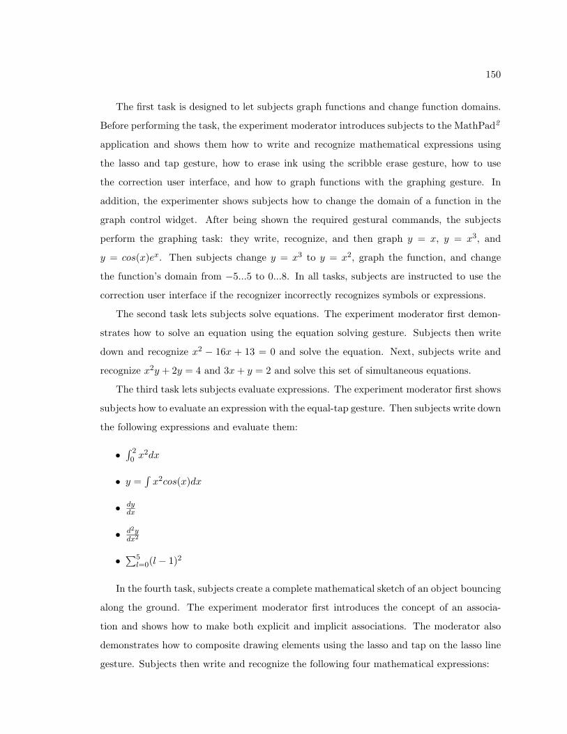
150
The first task is designed to let subjects graph functions and change function domains.
Before performing the task, the experiment moderator introduces subjects to the MathPad2
application and shows them how to write and recognize mathematical expressions using
the lasso and tap gesture, how to erase ink using the scribble erase gesture, how to use
the correction user interface, and how to graph functions with the graphing gesture. In
addition, the experimenter shows subjects how to change the domain of a function in the
graph control widget. After being shown the required gestural commands, the subjects
perform the graphing task: they write, recognize, and then graph y = x, y = x3, and
y = cos(x)ex. Then subjects change y = x3 to y = x2, graph the function, and change
the function’s domain from −5...5 to 0...8. In all tasks, subjects are instructed to use the
correction user interface if the recognizer incorrectly recognizes symbols or expressions.
The second task lets subjects solve equations. The experiment moderator first demon-
strates how to solve an equation using the equation solving gesture. Subjects then write
down and recognize x2 − 16x + 13 = 0 and solve the equation. Next, subjects write and
recognize x2y + 2y = 4 and 3x + y = 2 and solve this set of simultaneous equations.
The third task lets subjects evaluate expressions. The experiment moderator first shows
subjects how to evaluate an expression with the equal-tap gesture. Then subjects write down
the following expressions and evaluate them:
•∫ 20 x2dx
• y =∫
x2cos(x)dx
• dydx
• d2ydx2
• ∑5l=0(l − 1)2
In the fourth task, subjects create a complete mathematical sketch of an object bouncing
along the ground. The experiment moderator first introduces the concept of an associa-
tion and shows how to make both explicit and implicit associations. The moderator also
demonstrates how to composite drawing elements using the lasso and tap on the lasso line
gesture. Subjects then write and recognize the following four mathematical expressions:

151
Figure 10.4: The fourth task in the MathPad2 usability test.
• b = 5
• px(t) = t
• py(t) = abs(b sin(t))
• t = 0 to 20
Once these expressions are correctly recognized, subjects make a drawing with a horizontal
line representing the ground and a composite drawing element consisting of three circles
drawn near the start of the horizontal line. Next, subjects write the number 20 and associate
it to the horizontal line. Finally, subjects associate the mathematics to the composite
drawing element, either choosing an explicit association or using an implicit association
with the letter “p”, and run the sketch. Note that we have subjects make a composite
drawing element in this task so they are exposed to all the different lasso and tap gestures.
Figure 10.4 shows the complete mathematical sketch subjects create for this task.
In the fifth task, subjects create a mathematical sketch illustrating damped harmonic
oscillation. Since the main purpose of this task is to evaluate how well subjects make nails
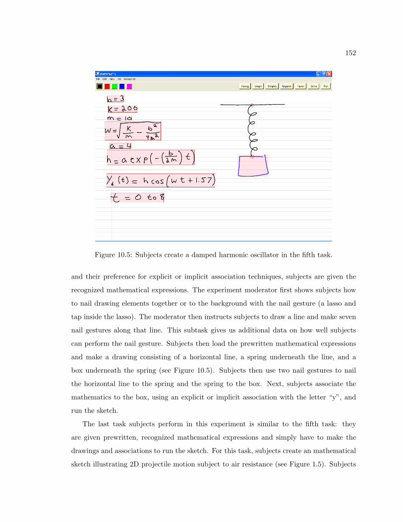
152
Figure 10.5: Subjects create a damped harmonic oscillator in the fifth task.
and their preference for explicit or implicit association techniques, subjects are given the
recognized mathematical expressions. The experiment moderator first shows subjects how
to nail drawing elements together or to the background with the nail gesture (a lasso and
tap inside the lasso). The moderator then instructs subjects to draw a line and make seven
nail gestures along that line. This subtask gives us additional data on how well subjects
can perform the nail gesture. Subjects then load the prewritten mathematical expressions
and make a drawing consisting of a horizontal line, a spring underneath the line, and a
box underneath the spring (see Figure 10.5). Subjects then use two nail gestures to nail
the horizontal line to the spring and the spring to the box. Next, subjects associate the
mathematics to the box, using an explicit or implicit association with the letter “y”, and
run the sketch.
The last task subjects perform in this experiment is similar to the fifth task: they
are given prewritten, recognized mathematical expressions and simply have to make the
drawings and associations to run the sketch. For this task, subjects create an mathematical
sketch illustrating 2D projectile motion subject to air resistance (see Figure 1.5). Subjects

153
first load the recognized mathematics and then draw a horizontal line and a ball near the
left side of the horizontal line. They then associate the number 100 to the horizontal
line. Finally, subjects associate the mathematics to the ball, using an explicit or implicit
association with the letter “p”, and run the sketch. Like the fifth task, this task is used to
gauge subjects’ preferences for the implicit or explicit association technique. After all six
tasks are completed, subjects answer a post-questionnaire (see Appendix B).
10.3.2 Participants
Seven subjects (four men and three women) participated in the MathPad2 usability eval-
uation. Subjects were recruited from the Brown University undergraduate population and
were either physics or applied mathematics majors. Subjects’ ages ranged from 19 to 23
and all were right-handed; only one had used a pen-based computer before (a PDA). All
seven subjects were asked prior to the study if they had used mathematical software before
and which packages: six subjects answering yes had used a variety of different packages
including Matlab, Mathematica, and Maple. All seven subjects had previously participated
in the mathematical symbol and expression recognizer accuracy study and were paid $30
for their time and effort in both studies.
10.3.3 Evaluation Measures
We evaluate MathPad2 ’s usability using quantitative and qualitative data from subjects’
task performances and from a post-questionnaire. As subjects perform the six experimental
tasks, the experiment moderator records important information about subjects’ perfor-
mances in completing each task and the decisions they made, and counts their mistakes.
Performance is characterized by whether subjects can complete each task and how well they
do on each subtask. Therefore, the moderator records whether or not subjects make the
appropriate gestures correctly and, if so, whether on the first attempt. Knowing how well
subject perform gestural operations on their first attempt is important because we want
to see how well subjects with little or no training can use MathPad2 . The moderator also
records subjects’ choices of implicit and explicit associations in tasks 4–6 so as to get a
quantitative metric for their preferences.
154
After subjects have completed all six tasks they are given a post-questionnaire (see
Appendix B) designed to get their reactions to MathPad2 ’s user interface and its perceived
usefulness, assess how well they remember certain gestures, and solicit their ideas for how
to improve the software. The first and second parts of the post-questionnaire, adapted from
Chin’s Questionnaire for User Interface Satisfaction [Chin et al. 1988], asks subjects to rate
MathPad2 ’s user interface as a whole and its individual components. In addition, subjects
were asked to comment on the correction user interface, which association technique they
preferred, and MathPad2’s most positive and negative aspects. In the third part of the post-
questionnaire, the recall test, subjects are asked to show what gestures they would use for six
different operations, indicating how easy MathPad2 ’s interface is to remember. The fourth
part of the post-questionnaire, adapted from the Perceived Usefulness portion of Davis’s
questionnaire for user acceptance [Davis 1989], asks whether subjects would use MathPad2
in their work. The final part of the post-questionnaire asks subjects what additional features
they would like to see in MathPad2 . After subjects answer the post-questionnaire, the
experiment moderator reviews it with them to make sure their answers are clear and to
elaborate further on any specific parts of MathPad2 .
10.3.4 Results and Discussion
The first task subjects perform in the MathPad2 usability study is writing, recognizing,
and graphing equations. Subjects were able to write and recognize all of the mathematical
expressions fairly easily. In some cases, they had to use the correction user interface to fix
recognition errors, generally getting MathPad2 to recognize their expressions on the second
or third attempt. A total of 28 graphing operations were performed (four per subject), and
subjects correctly graphed the expressions 27 times on the first attempt, for a first-attempt
performance of 96%. Subjects also had to change the domain of a graph; they all completed
this operation on the first attempt.
The second task is to write, recognize, and solve a simple equation and a set of simul-
taneous equations. As in the first task, subjects had little trouble writing and recognizing
the equations, although in some cases, it took two or three attempts to obtain a correctly

155
recognized equation. A total of 14 equation-solving operations were performed (two per sub-
ject), and subjects solved the equations 12 times on the first attempt, for a first-attempt
performance of 86%. The other two equation solves were correctly performed on the second
attempt.
The third task subjects perform is to write, recognize, and evaluate mathematical expres-
sions. Subjects had little difficulty in writing and recognizing the expressions and utilized
the correction user interface to fix recognition mistakes. A total of 35 expression evalua-
tions were performed (five per subject), and subjects evaluated the expressions 34 times on
the first attempt, for a first-attempt performance of 97%. One subject, however, did have
difficulty in recognizing d2ydx2 and even after multiple attempts was not able to evaluate the
expression.
The fourth task asks subjects to create a mathematical sketch of a bouncing ball, as
shown in Figure 10.4. All seven subjects completed the task and made the dynamic il-
lustration. However, three subjects had difficulty in writing and recognizing the required
mathematical specification and, after multiple attempts, were given prewritten expressions.
Subjects had no difficulty making the drawings and only once did a subject have trouble
making the composite drawing element. A total of 14 associations were made in this task
(two per subject) and subjects made 12 of them on the first attempt, for a first-attempt per-
formance of 86%. One subject had trouble with the associations and needed a few attempts
to make them correctly. The first association in this task is a label, and all seven subjects
used an implicit association. The second association is to associate the mathematics to
the composite drawing element; here subjects used an explicit association six times and an
implicit association only once.
The fifth task asks subjects to make a damped harmonic oscillator with prewritten
mathematical expressions (see Figure 10.5). All seven subjects completed the task and
made the dynamic illustration. Subjects needed nails for this task: seven nails on a drawn
line and two nails for the actual sketch. A total of 63 nails were made in this task; subjects
made 56 of them on their first attempt, for a first-attempt performance of 88%. Most of the
remaining nails were made on the second attempt. However, one subject required several
attempts to make the necessary nails and had to recreate the drawing after inadvertently

156
Overall Reaction to MathPad2
Mean Std. Deviation
Terrible=1, Wonderful = 7 6.42 0.54
Difficult=1, Easy=7 5.57 0.98
Frustrating=1, Satisfying=7 5.57 1.13
Dull=1, Stimulating=7 6.14 0.38
Table 10.2: Subjects’ average ratings of their overall reaction to MathPad2 on a scale from1 to 7.
erasing part of it when erasing an incorrectly recognized nail. As in the fourth task, subjects
had no difficulties in making the drawings. Subjects had to make one association in this
task, and all seven used an explicit association.
The sixth task asks subjects to make a mathematical sketch to illustrate 2D projec-
tile motion with air resistance using prewritten mathematical expressions (see Figure 1.5).
All seven subjects completed the task and made the dynamic illustration. Subjects made
the drawings without difficulty and needed to make two associations consisting of a label
association and a mathematical specification association. All 14 associations were made im-
plicitly. One subject had some difficulty with the implicit associations and needed several
attempts to make them correctly.
Overall, subjects did well on all six tasks, considering that they had no hands-on train-
ing beforehand. In only one case did a subject not complete part of a task and this was
due to the inability to recognize an expression correctly. The first-attempt performances
are high considering that subjects had not practiced any of the gestural commands. One
subject did have some difficulty with implicit associations due to problems with making
taps. The greatest problem subjects had with the six tasks was obtaining correctly rec-
ognized expressions in certain situations. That three out of the seven subjects required
prewritten mathematics for task four shows that the mathematical expression recognizer
needs improvement.
After the six tasks were completed, subjects were given a post-questionnaire. The first
part of the post-questionnaire asks subjects to comment on their overall reaction to the
MathPad2 application. Table 10.2 summarizing these results shows that subjects had a
positive reaction to MathPad2 . When subjects were asked why they chose their rankings,

157
MathPad2 User Interface Ease of Use
Mean Std. Deviation
Writing Mathematics 1.43 0.97
Recognizing Mathematics 2.57 1.81
Graphing Functions 1.0 0.0
Solving Equations 1.0 0.0
Evaluating Expressions 1.0 0.0
Grouping Drawing Elements 1.57 0.79
Making Associations 1.71 0.76
Making Nails 1.57 0.59
Table 10.3: Subjects’ average ratings of ease of use for different components of the MathPad2
user interface (scale: 1=easy, 7=hard).
most asserted that MathPad2 works well, is easy to use, and would be very useful for
students in a classroom setting and/or doing homework problems. One subject was amazed
at the application’s power. Two subjects claimed MathPad2 was easy to use but could be
frustrating when it had trouble recognizing their handwriting; this frustration explains why
the second and third rankings in Table 10.2 are slightly below the first and fourth rankings.
The second part of the post-questionnaire gauged MathPad2 ’s ease of use. Subjects
rated different parts of the MathPad2 user interface from 1 (easy) to 7 (hard). Table 10.3
summarizes these results and shows that subjects found MathPad2 easy to use. Subjects
gave recognizing expressions the highest average ranking, indicating the fact that some
users had trouble getting MathPad2 to recognize their handwriting. When asked about
their ranking, they stated that the gesture for recognizing mathematical expressions (i.e.,
lasso and tap) was easy to use, but the results of the recognition operation led them to
choose a higher ranking on the easy (1) to hard (7) scale.
Subjects were then asked two questions directly concerning MathPad2 ’s user interface.
First, they were asked which type of association method they preferred and why. All seven
subjects preferred explicit associations, claiming they were easier to remember and simpler
and faster to perform. However, they did say that when associations need to be made
with a drawing element and a large set of mathematical expressions, the implicit method
is more appropriate. We can thus conclude that both association methods have their place
in mathematical sketching. Second, subjects were asked if the correction user interface

158
helped them fix recognition mistakes; five out of the seven subjects answered yes to this
question. The two subjects who said no claimed that the alternate lists gave them no help
in correcting recognition errors. One subject wanted more choices to appear in the alternate
lists, especially in the equation alternate list.
Subjects were also asked for the most positive and negative aspects of MathPad2 ’s
user interface. Most subjects identified the most positive aspect as its ability to quickly
make drawings move as described by mathematical equations. Two subjects claimed that
solving equations was one of the user interface’s most positive aspect. One subject thought
that the best part of MathPad2 ’s user interface was the scribble erase command; another
subject said the user interface’s simplicity was its most positive aspect. Three subjects
stated that getting MathPad2 to recognize certain symbols and equations correctly was the
most negative aspect of the user interface. Two subjects stated that the lack of interactive
feedback for implicit associations was a significant drawback, and one subject stated that a
negative aspect was the time necessary to get used to the gestural commands. Finally, two
subjects said that MathPad2 ’s user interface had no negative aspects.
Subjects were then asked to rate MathPad2 ’s overall ease of use on a scale from 1 (easy)
to 7 (hard). On average, subjects gave MathPad2 a 1.86 with a standard deviation of
0.69. When they were asked to explain their ratings, two dominant themes emerged. First,
subjects found the interface easy to use and remember, but were in some cases frustrated by
problems in mathematical expression recognition. However, the subjects who had trouble
with recognition all felt it would improve with more practice. Those subjects were also
asked if they would still use MathPad2 in spite of their recognition problems; they all said
they could deal with these problems because of the functionality MathPad2 would give
them. Second, subjects felt the interface was easy to use once it was explained, a result
expected given MathPad2 ’s gestural interface.
The third part of the post-questionnaire asked subjects to remember how to invoke
gestural commands for graphing, solving equations, evaluating expressions, recognizing a
mathematical expression, making nails, and making implicit associations. Subjects an-
swered 38 out of the 42 recall questions correctly (six per subject) for a recall rate of 90%.

159
MathPad2 Perceived Usefulness
Mean Std. Deviation
Accomplish Tasks More Quickly 5.14 1.95
Improve Performance 4.71 2.36
Increase Productivity 5.0 1.91
Enhance Effectiveness 5.14 2.04
Easier To Do Work 5.57 1.90
Useful In Work 5.42 2.37
Table 10.4: Subjects’ average ratings of the perceived usefulness of MathPad2 in their work(scale: 1=unlikely, 7=likely).
Of the four questions subjects answered incorrectly, three subjects missed the solving equa-
tion gesture (squiggle) and one missed the expression evaluation gesture (equal and tap).
The 90% recall rate indicates that subjects had little difficulty remembering MathPad2 ges-
tures except for the equation solving gesture. Even though three out of the seven subjects
forgot the equation solving gesture, they still found it easy to use.
The fourth part of the post-questionnaire asks subjects how likely they would be to
use MathPad2 in their work. Table 10.4 summarizes subjects’ ratings on the different
“perceived usefulness” statements, on a scale of 1 (unlikely) to 7 (likely). Most subjects
would use MathPad2 in their work. When asked to explain their ratings, four subjects
stated that the application would help them to do their classwork and obtain a better
understanding of problems and concepts. However, there was no consensus on whether
MathPad2 would speed their understanding of these problems and concepts. One subject
said that the ability to quickly solve equations and make graphs would be very beneficial.
Two subjects said they did not think they would use MathPad2 in its current form in
their work (explaining the high standard deviations in Table 10.4). Both of these subjects
work in theoretical physics, one in optics and the other in modern physics. However, one
of these subject stated she would have used MathPad2 during beginning physics classes
while the other stated he would use MathPad2 if it had support for light ray and optics
diagrams. Finally, all seven subjects felt the application would be a good tool for teachers
of introductory mathematics and physics classes.
The last part of the post-questionnaire asked subjects to list features they would like

160
to see in MathPad2 . These features can be divided into application-control features and
mathematical sketching and tool improvement. For application control, subjects want to be
able to rewind a dynamic illustration and move interactively from the beginning to the end of
the simulation. In addition, they want graph drawing element trajectories, vector support,
more screen space, and the ability to elongate square roots and fractions if their lengths
are underestimated when writing mathematical expressions. In tool improvement, subjects
want to make 3D graphs, phase portraits and other visualizations used in chaos theory,
to use complex numbers and do Fourier analysis, and to draw paths and have MathPad2
generate equations. In mathematical sketching, subjects were interested in seeing support
for illustrations using partial differential equations, electromagnetic fields and flux, and
optics (e.g., lens and ray diagrams). All of these ideas are part of future work.
The results of the MathPad2 usability study suggest that the application is, in general,
easy to use. Most gestures are easy to remember, and subjects found the application a
powerful tool that beginning physics and mathematics students could use to help solve
problems and better understand scientific concepts. Some subjects performed the tasks
with little trouble, while others had some difficulty, stemming primarily from problems
with mathematical expression recognition. However, these subjects also said they were
willing to accept these recognition problems given what MathPad2 can offer them, and also
thought the recognition would improve with more practice.
Nevertheless, we need better mathematical expression recognition that will perform
robustly across a larger user population. A better correction user interface could also
go a long way to helping with users’ frustrations when incorrect recognitions occur (see
Section 11.2.2). In addition, more interactive feedback is needed for implicit associations,
and the equation solving gesture may need to be redesigned. These results also show that
mathematical sketching should support many more application features and different types
of dynamic illustrations.

Chapter 11
Discussion and Future Work
Previous chapters have discussed the components of mathematical sketching and presented
a usability study on MathPad2 , a prototype mathematical sketching application. Here we
discuss mathematical sketching further and present an agenda for future work in all aspects
of the paradigm. In addition, we discuss the plausibility of much of the future work.
11.1 Discussion
In addition to the usability evaluation described in Chapter 10, MathPad2 has been shown
to people from college students to professors to corporate executives. Our discussions with
them and their perceptions of the application, as well as our own analysis, have yielded
some observations about various issues with and limitations of mathematical sketching.
This section discusses these current issues and limitations as a prelude to some of the
future work discussed in Section 11.2.
11.1.1 Further Observations
The current version of MathPad2 has some inflexibility in the mathematics users can write
when making mathematical sketches and invoking symbolic or computational tools. For
example, graphs can be functions only of x or t, and users can solve only equations that
contain x, y, z, or w as variable names. These restrictions stem from our use of MathPad2
as a prototype to test out the mathematical sketching paradigm. In most cases, these
restrictions create little difficulty since users can still invoke operations on a wide variety of
161

162
mathematical expressions. However, a more robust version should remove these restrictions.
MathPad2 is also somewhat inflexible in certain mathematical expressions, specifically those
that are undefined in certain parts of their domains (e.g., 1(x+1)(x−1)); while this inflexibility
is unimportant in evaluating the mathematical sketching paradigm, in a more robust setting
users would need to be able to use these types of expressions.
Units make it easier to specify mathematical and physical phenomena, but mathematical
sketching does not currently support them. While users can remember units or write them
down but not recognize them, this approach is not a valid solution. On the basis of how
users work to solve mathematical and physical problems and how they are presented in
various textbooks, we believe that providing unit support will go a long way toward making
mathematical sketching more usable. Unfortunately, supporting units is a difficult problem.
For example, consider the expression 9.8m/s2. This expression has a high level of ambiguity:
it could mean 9.8 times m divided by s2 or 9.8 meters per second squared. Having an
internal representation for units and looking for this type of notation would restrict a user’s
expressive power. Another approach would be to have users select units from a pull-down
menu, or create a special location where units are written. Regardless of the approach,
units need to be supported in mathematical sketching in one form or another.
One of our important observations about how mathematical sketching works concerns
problems that are not primarily motion-based but could have motion given further deriva-
tion. Consider a concrete block suspended from several wires. The question is to find the
forces affecting each wire, given the mass of the block. This problem is not necessarily
motion-based, but if the forces acting on the wires are calculated incorrectly, it is possible,
given the tension thresholds for the wires, that one or more wires would break, causing the
block to fall to the ground. Thus, motion is possible given an incorrect calculation, but is
more of an aftereffect than a primary part of the problem. Such scenarios are supported in
mathematical sketching but would require mathematics that is not necessarily part of the
problem. Making these types of problems easier to deal with is an important part of improv-
ing mathematical sketching; having higher-level encapsulated mathematical constructs or
an underlying physics engine (e.g., rigid body simulator, Newtonian mechanics simulator)
could be a solution.

163
The very nature of mathematical sketching makes dealing with sketch correctness chal-
lenging. Because users make free-form drawings instead of creating precise geometric primi-
tives, mathematical sketching tends to create approximate dynamic illustrations. Therefore,
users can often verify only approximately that their mathematical specifications are correct.
For the most part, this is sufficient. However, in some cases, especially those that use open-
form solutions, it might be difficult to know without verification tools if the specification
is correct. These verification tools (e.g., visual debugging tools) remain an open research
problem in mathematical sketching that needs to be addressed.
Mathematical sketching is inherently a pen-based activity. More specifically, it is an
activity that works best when users have screen-based tablets because these devices closely
mimic pencil and paper. The drawback of screen-based tablets is they are not common input
devices, limiting MathPad2 ’s potential use. Nonscreen-based tablets are far more common
than their screen-based counterparts, but with such tablets, users have to look up at the
screen to get feedback on their writing, an unnatural task. In fact, MathPad2 was first
tested with a nonscreen-based tablet and was found to be unsuitable without significant
training. Nevertheless, it is important to investigate further how to let users with these
tablets use MathPad2 .
The MathPad2 application has a practical limitation: it has only one piece of virtual
paper for users to make mathematical sketches on. Many users and observers of MathPad2
have commented on the need for more space to create mathematical sketches. Although
this seems like trivial functionality to add to MathPad2 , some important considerations
are involved. In a traditional notebook, users have multiple pages: when they are finished
with one they simply go on to the next. This notebook-style approach seems logical for
MathPad2 . However, the problem is that users have to flip back and forth among pages.
Another approach is to use a large piece of virtual paper, with the display screen acting as
a window onto parts of it. Users could then move this window around to see more of the
virtual paper or use zooming tools to fit more of it in the window. Both approaches need
to be explored in future versions of MathPad2 .
Finally, we found that looseleaf or graph-paper backgrounds instead of a plain white

164
background were helpful to users when making mathematical sketches. This sort of struc-
ture made it easier for users to write mathematical expressions with straight baselines and
to make straight lines in their free-form drawings. As MathPad2 improves, other types of
backgrounds can be added, such as graph paper with varying scales or for different coordi-
nate systems.
11.1.2 Current Limitations of Mathematical Sketching
The current version of mathematical sketching lets users make dynamic illustrations in which
drawing elements are animated based on affine transformations or stretched as a result of
affine transformations. Thus, mathematical sketching supports any dynamic illustration as
long as users can write or derive mathematical specifications that define drawing elements’
affine transformations. Although mathematical sketching supports many different types of
dynamic illustrations, it does have limitations as implemented in MathPad2 .
The current version of mathematical sketching does not permit nested iterations or
multi-statement conditionals. The lack of nested iterations could make more sophisticated
numerical techniques difficult to specify. A multi-statement conditional is one that can
have more than one statement after each logical expression. MathPad2 does not support
this more complex construct and, as a result, it is difficult to write all but the simplest
conditionals. Higher-level mathematical constructs are also not supported in the current
version of mathematical sketching. Mathematical sketching is designed so that users fully
specify the mathematics used to animate drawing elements, but in some cases, this approach
may not be appropriate. As an example, consider the concrete block suspended from tension
wires discussed in the previous section. We could animate the tension wires breaking and
the block falling to the ground if the system is not in equilibrium, indicating that the
user’s force calculations are incorrect. In the current implementation, a user could define
the force equations and doubly integrate them to get a displacement function. However, if
mathematical sketching understood the concept of F = ma, it could perform the necessary
computations without the user having to specify all the mathematics that are not part of
the problem.
The current version of mathematical sketching also has several limitations in terms of

165
free-form drawings and their relationships to the mathematics. First, complex animation
relationships can be difficult to handle. As an example, consider a block sitting on an
inclined plane. In order for the block to slide down the plane, we need the appropriate
mathematical specification with the appropriate transformed coordinate system to ensure
the block does not deviate from the plane’s incline. Creating a constraint between the
block and the plane would make the specification easier, but MathPad2 does not currently
support this functionality. Along the same lines, drawing elements can be stretched, given
they are attached to drawing elements with associated affine transformations, but they
cannot follow constrained motion easily. As an example, given two blocks attached to a
string on a pulley system, users would have difficulty in making the string move about
the pulleys without deriving a complicated mathematical specification. Once again, adding
some type of constraint could lessen the user’s burden in cases when the focus of the
mathematical sketch is not directly on the pulley’s interaction with the string. Finally, the
current version of mathematical sketching does not support repeatable drawing element
animation: users cannot easily have more than one drawing element move in succession
(e.g., multiple projectiles, shot out of a cannon, one after another).
Dynamic illustrations created with mathematical sketches cannot currently generate
ink during an animation. In other words, mathematical sketching only animates drawing
elements that have already been drawn on the screen. Having ink creation during an ani-
mation would enhance mathematical sketching significantly, by supporting more traditional
visualization techniques. For example, motion traces for moving drawing elements could
be used as another visual aid in exploring mathematical or physics concepts. Many types
of electrostatic and magnetism problems could also be explored if the dynamic illustration
could generate field lines during the animation. The concept of a “laser beam” would let
users create optics and ray diagrams so that the beam, an increasingly larger ink stroke,
could emanate from a source and interact with lenses and mirrors.
11.2 Future Work
Because mathematical sketching is a new and relatively large-scale interaction paradigm,
a significant amount of future work should be explored. This section presents a research

166
agenda for mathematical sketching.
11.2.1 Plausibility Concerns
We attempt to go beyond simply stating what the future work in mathematical sketching
should be. We also discuss the plausibility of the ideas to give the reader a better under-
standing of the possibilities and pitfalls of each one. In addition, we provide some direction
on how to begin exploring each area of future work. We also estimate whether each area of
future work simply requires software development, is a research problem, or something in
between.
11.2.2 Improving Mathematical Expression Recognition
The analysis of the mathematical expression recognizer in Chapter 10 shows that improving
all phases of recognition accuracy is critically important in making mathematical sketch-
ing more usable. Thus more work needs to be done in mathematical symbol recognition,
mathematical expression parsing, how results are presented to users, and improving the
correction user interface.
Mathematical Symbol Recognition. A good way to improve the mathematical ex-
pression recognizer as a whole is to improve the mathematical symbol recognizer. Greater
symbol recognition accuracy is important in and of itself but also helps to improve math-
ematical expression parsing. One way to improve mathematical symbol recognition is to
detect how symbols are written when users provide handwriting samples. In some cases,
users may write certain symbols (e.g., “y” or “p”) with one or more than one stroke during
training. Having the recognizer detect this and make multiple templates would improve
recognition. However, the number of training samples for a particular symbol would have
to be divided on the basis of how the symbol was written, which would reduce the amount
of data for each class of that symbol. Of course, we can simply ask users to provide more
samples for that symbol. Extending the symbol recognizer to support multiple templates
per symbol is straightforward, a minimal software development effort.
Another approach to improving mathematical symbol recognition is to increase the
167
number of samples users must provide per symbol, but this extra burden increases users’
startup costs. A possible strategy would be to keep the same number of training samples as
before (perhaps even reduce it) but use an incremental learning algorithm [Duda et al. 2001,
Giraud-Carrier 2000] so that the recognizer learns as users write mathematical expressions.
We believe that an online or incremental learning algorithm can greatly improve recognition
performance as users work with the recognizer because it will continuously adapt to users’
handwritings. In fact, it would be possible to start with an independent recognizer and
have it adapt to particular users. Since users would provide samples to the recognizer as
they use the system, they would perceive the recognizer as independent, but it would evolve
into a dependent recognizer without any user startup costs.
The two key factors in making incremental learning plausible are choosing an incremental
learner and devising how to send users’ written symbols to it with as little user intervention
as possible. We could use any of the different learning algorithms that are suitably adapt-
able to incremental learning (see [Duda et al. 2001] for some examples). AdaBoost is one
possibility that makes sense, given that it is already part of our current symbol recognizer.
We must ensure that its learning does not interfere with what users are doing within the
context of the application. One way to handle this problem is to have the application store
correct recognition results and retrain the learner with the additional data after users quit
the application; when users start the application again, it will have incorporated the last
session’s data. Taking the approach that the incremental learner retrains only after users
quit the application is simply a matter of extending our current recognizer, requiring a
moderate amount of software development. However, having the symbol recognizer retrain
as users interact with the system is a moderately challenging research problem because we
have to ensure that the incremental learner can retrain quickly and not interfere with user
interaction flow.
Another important issue is how users tell the system that recognized symbols should be
treated as additional training data. Ideally, users would write, recognize, and correct any
handwritten symbols and the system would determine which symbols to add to the training
set with no user intervention. The drawback of this approach is that, given mathematical
sketching’s correction user interface, it is difficult to know whether users are correcting a
168
misrecognized symbol or changing a correctly recognized symbol in the course of modifying
an existing mathematical expression. We could have users explicitly tell the system that
they made a correction, perhaps by tapping on the green button in the lower right corner of
recognized expressions’ bounding boxes, tapping on some other predefined button, or hav-
ing a preset gesture. Providing a seamless, invisible user interface for informing the system
that user-corrected symbols should be additional training data is a moderately challenging
problem in user interface research.
Mathematical Expression Parsing. Improving mathematical expression parsing
is also an important area for future work, since more accurate parsing will also greatly
improve the usability of mathematical sketching. The parsing algorithm is currently writer-
independent (except for ascender and descender symbol information), but the variability
with which users write symbols makes an independent approach problematic. One way to
deal with this problem is to have users write a set of mathematical expressions to train
the parsing algorithm; at a minimum, these samples could be used to define the 2D spatial
relationship rules. A more sophisticated approach would be to use the stochastic grammar
approach described in Section 6.2. Regardless of the approach, however, users would have
to provide sample mathematical expressions to train the parser, and designing this training
set is not trivial. Since users often write symbols at different scales depending on their
context in a mathematical expression, there are many different ways in which symbols can
relate to one another. Moreover, even with a reasonable training set of mathematical ex-
pressions for the parsing algorithm, we do not want to increase users’ startup costs. One
approach that is in line with the incremental mathematical symbol recognizer is to use the
2D spatial relationship rules already in place and have the algorithm adapt to how users
write mathematical expressions as they use mathematical sketching. We believe that having
a mathematical expression recognizer (symbol and parsing recognition) that incrementally
learns users’ handwritings will significantly increase accuracy. Using a stochastic gram-
mar or incremental learning approach to improve the parsing algorithm would requires a
significant amount of software development given our current parsing algorithm. Finding

169
Figure 11.1: Our current conditional parsing algorithm fails to parse this expression cor-rectly. By looking at pairs of symbols, we could construct a polyline (the red line in betweenthe two statements) to separate the two statements so they can be parsed correctly.
a reasonable, statistically valid set of mathematical expressions to train the parsing algo-
rithm on is a moderately difficult research problem due to the variability in how users write
mathematical expressions.
Another potential improvement of the parsing algorithm concerns parsing conditionals.
The parsing scheme for conditional expressions looks for horizontal lines between expressions
to break up the conditional into separate statements. Using horizontal lines is somewhat re-
strictive and unless the conditional is written neatly with space between statements, parsing
errors will occur. We could make conditional rule less restrictive by using polylines instead
of horizontal lines to break up the conditional expression. This approach would handle
cases where the space between two statements is curved (see Figure 11.1). We could also
extend this approach to handle all the mathematical expressions on a page. Currently,
users must lasso and tap each mathematical expression to recognize it. With this more
flexible conditional expression parsing approach, users could simply press a button or make
a simple gesture that would segment the symbols on the page into expressions and then rec-
ognize them. This less restrictive parsing approach requires a minimal amount of software
development for dealing with conditionals but may require more research, given a page of
mathematical expressions because of more complex layouts.
Mathematical Expression Recognizer Output. When users invoke the mathemat-
ical expression recognizer, the recognized symbols are presented in the users’ own handwrit-
ings but the parses are not. Users have to click on the small green button in the lower right

170
corner of the expression’s bounding box to get a 1D representation of the recognized ex-
pression. This approach is clearly a limitation and an area for future work. While we could
typeset the results and present them to the user, we want to maintain our notebook “look
and feel” so a better solution is to present the parsing results in the user’s handwriting: if
the expression was recognized correctly, users would see little if any change in the written
expression. To do this task, we would need information on how users write mathematical
expressions so the expression’s spatial relationships could be maintained, but getting this
information goes back to the need for training samples provided by each user and all the
issues that entails. One compromise would be simply to present the parsing results on the
basis of the 2D spatial relationship rules; this approach would also show users how to write
mathematical expressions so they are parsed correctly. Presenting the parsing results to
users based on the current 2D spatial relationship rules is a fairly straightforward software
development effort. However, presenting the results in the user’s own writing style requires
more work because mathematical expression samples are needed from each user.
The Correction User Interface. We also plan to improve the correction user in-
terface. Even with significant improvements in the recognizer, mistakes will invariably be
made, and a powerful correction user interface will make mathematical sketching more us-
able. The two main areas in which the correction user interface can be improved are parse
correction and the generation of alternate expressions. Currently, users can correct parsing
mistakes by lassoing one or more symbols and dragging them to a different location so that
the recognizer reparses the expression. However, currently users do not have a good idea of
exactly where to place the symbol or symbols to correct the error. We need to provide more
feedback. We could highlight regions where symbols should be placed for certain constructs.
For example, if a user wants to take the 2 in x2 and move it up so the expression becomes
x2, as the user moves the 2 towards the superscript position, the region to the upper right of
the x could highlight to show exactly where the 2 should go. A drawback of this approach is
that the number of possible locations where a symbol or symbols could be placed increases
as the mathematical expression becomes more complex. However, even with very complex
171
expressions, this feedback would help to reduce the number of incorrectly recognized expres-
sions. An extension of this type of feedback would be to highlight relevant symbol regions
as users write mathematical expressions. However, this would require recognition in real
time as users wrote the mathematics. Adding these extensions is a straightforward software
development effort.
We also would like to improve the generation of alternate expressions. Generating a
proper set of alternate expressions is a challenging research problem because more and
more different combinations become possible as the complexity of the expression increases.
The key would be to come up with a reasonable subset of alternate expressions, not a
trivial matter. We could keep track of all the spatial relationship tests, choose the ones
whose results are close geometrically, and generate alternate expressions on the basis of
what has come before (e.g., subscripts, superscripts, etc.). If incremental learning is used in
the parsing step, we can also use information on the parsing errors users correct to see what
a particular user’s the most common parsing errors are and generate alternate expressions
based the parsing correction data.
11.2.3 Expanding Mathematical Sketching
In this section, we discuss a variety of ideas for expanding mathematical sketching, including
• Improving the computational and symbolic toolset
• Improving drawing dimension analysis
• Improving drawing rectification
• Allowing saveable functions and macros
• Supporting matrix and vector notation
• Moving to 3D
• Increasing interactivity
• Generating mathematics from drawings

172
• Adding specific underlying mathematical engines
The Computational and Symbolic Toolset. Graphing mathematical expressions
is currently restricted to two-dimensional line plots. Extending graphing functionality to
support other types of graphs such as histograms, 3D line plots, and contour and surface
plots in 2D and 3D would increase mathematical sketching’s flexibility. Adding these new
types of graphs would not add much complexity to the interface. Using the graphing
gesture, the system could analyze the mathematical expressions to determine what type
of graph to create. In some cases, several types of graphs could be made for a given
mathematical expression: adding a simple marking [Kurtenbach and Buxton 1994] or flow
menu [Guimbretiere and Winograd 2000] to the graph gesture would let users choose which
type of plot they wanted if multiple plot styles were available. Mathematical sketching
also needs to support plotting function families. For example, a solution to an ordinary
differential equation is a family of functions based on the constants in the solution. If
initial conditions are provided, the solution is simply one function (assuming no other
constants are present). Having the system choose a reasonable range for these constants
so the general solution to an ordinary differential equation can be visualized would greatly
improve mathematical sketching. Users could also specify these ranges for more interactive
control. Another limitation of mathematical sketching’s current graphing approach is that
a function’s domain is predefined in the graph. Users can adjust a function’s domain in
the graph widget by writing in the values, but an automatic way to choose an appropriate
domain might be more useful. One approach to finding an appropriate domain would be
use the zeros of the function as a guide, but this approach would work well only in some
cases.
More flexibility in expression evaluation and equation solving will also increase the power
of mathematical sketching. Currently, users make an equal and tap gesture next to a recog-
nized mathematical expression and the expression’s context determines whether integration,
summation, differentiation, or simplification should be performed. Extending expression
evaluation to support additional numerical calculations as well as other symbolic manip-
ulation such as factoring, Fourier transforms, and Taylor series expansions would make it
difficult simply to rely on the expression’s context for its evaluation. Using either marking or

173
flow menu techniques as part of the equal and tap gesture would help to distinguish among
the multitude of different evaluation options while still maintaining the user interface’s flu-
idity. In equation solving, mathematical sketching assumes it will solve for x, y, z, and w
if these variables are present in the equations. However, users may want to define a set
of equations with unknown constants and solve in terms of them. Improving the interface
for invoking equation-solving operations would let users choose what variables to solve and
thus provide more flexibility. A way to support this additional functionality would be to
turn the equation-solving gesture into a compound gesture by which users could explicitly
write in the variables to solve for, resorting to a default scenario if no variables are written.
Adding more functionality to the symbolic and computational toolset is a moderately dif-
ficult software development effort because additional gestures may be required that must
not conflict with mathematical sketching’s current gesture set.
Results from equation solving and expression evaluation is currently output using Mat-
lab 1D syntax. To maintain the notebook “look and feel” of the mathematical sketching
interface, output from these operations should be presented to users as 2D mathemati-
cal expressions as if they had written them down. Adding this functionality requires an
understanding of the Matlab syntax (so extra symbols can be removed) as well as strate-
gies for proper size and placement of the symbols. In effect, a 1D-text-expression-to-2D-
handwritten-expression-parser is required which will require a moderate amount of software
development due various parsing and display intricacies.
Drawing Dimension Analysis. Problems can occur during drawing dimension anal-
ysis when defaults are used or dimensions are overspecified. Two areas of future work for
improving drawing dimension analysis are thus to devise better defaults and to create a
scheme for dealing with too much dimensional information. Currently, when no labels are
associated with drawing elements, the default used to define the simulation-to-animation
transformation works in some cases but fails in others.
A better solution, in the absence of label information, would be to use the data generated
from the Matlab code and to define dimensions in the x and/or y coordinate. This solution
is plausible if we can infer information about the drawing element’s geometry as it moves

174
through time. Given an animatable drawing element, we know its size in pixels in both the
x and y directions, its initial location in pixels and in simulation space, and its location
furthest away from the initial location. The difficulty is that we do not know how big
the drawing element is in simulation space without explicit labeling, since it is essentially
an underconstrained problem. Therefore, the best we can do is use the distance defined
by the minimum and maximum values in the x and/or y directions to create lengths for
the simulation-to-animation transformation. This transformation must be checked to see
if the drawing element’s transformed points go beyond the display’s boundaries; if so, the
transformation must be reduced so the animation fits nicely on the screen. At the other
extreme, the lengths defining the simulation-to-animation transformation could be so small
that the drawing element will move not at all or very little during the illustration. If so,
the transformation must be expanded (using the screen’s dimensions as a guide) so that the
animation looks reasonable.
The above approach would work if there is only one animatable drawing element. If there
is more than one, the problem is overconstrained since there is more than one possible way
to define the simulation-to-animation transformation. This difficulty also arises when more
than one drawing element is labeled with dimensional information in the x or y direction.
One approach, simply to define multiple transforms for each animatable drawing element,
does not work well in cases where moving drawing elements interact. A better solution
is to simply choose one transformation from the different possibilities for the x and/or y
direction. We could use the first label written for either axis to create the transformation.
If no labels are found, then the Matlab data and size of the display screen would define
the dimensions. Alternatively, we could choose the last labels written, or choose the labels
that best fit the display screen, so that the animation is always visible to the user. All
these approaches are plausible and require further analysis to choose among them. Since
there are many possible approaches for improving drawing dimension analysis and both
underconstrained and overconstrained situations occur, this is a moderately challenging
research problem.
Another issue is that the directions of the x- and y-axis are predefined, but it sometimes
makes sense to define these directions differently. For example, a coordinate system with
175
the x-axis parallel to an inclined plane makes it easier to specify the mathematics describing
the motion of an object moving along the plane. Users could specify different coordinate
systems by using a simple coordinate system widget: users could move this widget into the
correct orientation and then drag it onto the appropriate drawing element. Note that users
could specify the mathematics to move an object along an inclined plane without such a
tool, but the specification would have to reflect the rotated coordinate system. Adding a
coordinate system widget would take minimal software development effort.
Drawing Rectification. Drawing rectification is critical to making dynamic illustra-
tions look plausible and we currently support angle, location, and size rectification. Our
current approaches work well in many cases, but further improvement is needed.
Our current angle rectification procedure can cause problems with drawing elements,
such as breaking elements or creating multiple courses of action in maintaining drawing
element structure. The issues arising in angle rectification can be handled in two ways.
The first, employing a constraint solver, would help alleviate many angle rectification issues
but is a considerable engineering effort that adds complexity to mathematical sketching.
The constraint solver could present different solutions for users to pick from, giving them
flexibility in how they define their drawing elements. The other approach is to define a set
of rules for angle rectification to which users would simply adapt. From a user interface
perspective, the former approach seems more plausible, but an important area of future
work is to evaluate the two.
One of the important aspects of location rectification is where to relocate a drawing
element given more than one line label. If the animatable drawing element is close to
a given labeled line, we can use that line as the origin for rectifying the location. This
problem occurs in conjunction with drawing dimension analysis because the simulation-to-
animation transformation could be taken from labeled lines that differ from the one used
for location rectification. One possible solution is to simply have different transformations
for each animatable drawing element and use different origin points in rectifying location.
This solution will work if only drawing elements do not interact with one another. As with
drawing dimension analysis, using one common transformation seems a better approach, and

176
the issues and strategies discussed for drawing dimension analysis pertain here as well. Use
of a common origin point is not so obviously desirable: users may want different drawing
elements to use different origin points for relocation. These different locations could be
defined with the mathematics or by extending the association mechanism.
Many of the same issues of multiple line labels and dimension analysis come up with
size rectification as with location rectification, so that the possible approaches to location
rectification issues could also apply here. An issue different from location rectification is
that size rectification requires user intervention: users must supply a size value using the
animatable drawing element’s core label and a key letter in the label’s subscript. There are
other approaches to defining size information, for example using an interaction approach
similar to implicit associations: instead of a lasso and tap, users could lasso the value and
then draw a line on the drawing element to indicate whether the value indicated width,
height, or uniform size.
Location and size rectification use the center point of the drawing element, but users
may want to use a different point. For example, a user might draw a car and want its
front to be the rectification point when its location is rectified, or might want the car’s size
rectified using the back of the car as the scaling point. Mathematical sketching does not
currently let users make such choices. We could use the association techniques to provide
the necessary information for this functionality. Currently, when users lasso a core label
and tap on a drawing element to make an association, the tap location is used only to tell
the system that the tapped drawing element is the one in the association. The tap location
could be given a dual meaning so as to provide the point for size or location rectification.
An analysis of how difficult this technique is to remember would be needed to ensure the
plausibility of this approach.
In general, drawing rectification is a difficult problem that goes beyond drawing ele-
ments’ angles, locations, and sizes. Often, the free-form drawings themselves can cause
difficulties in making a dynamic illustration plausible. Dealing with this problem may in-
volve rectifying drawing elements on the level of stroke geometry, requiring higher-level
geometric primitives. It may be possible to recognize free-form drawings as more precise
geometric primitives (e.g., circles, rectangles, triangles, etc.), and use them to influence

177
Figure 11.2: How a user might specify a user-defined function. The def and end keywordssignify the start and end of the function respectively.
drawing element animation. All of these issues imply that drawing rectification is a signifi-
cantly challenging research problem.
Functions and Macros. Letting users define their own functions and macros would
make mathematical sketching more powerful because users could build libraries of specific
reusable functions. For example, a user could create a Runge-Kutta function for use in
sketches requiring open-form solutions, or define a function to encapsulate a rotation or
scaling operation. Users can already define simple functions when making mathematical
sketches to a certain extent, but they cannot store them and reuse them at will.
The key issue in user-defined functions and macros is how and at what level they are
specified in mathematical sketching. In general, users should be able to specify the func-
tion name, its input parameters, the statements that make up the function, and its output
parameters. These user-defined functions and macros could also become relatively sophis-
ticated in terms of whether function parameters can be passed by value or by reference.
One approach to defining functions and macros is to use a keyword to indicate that a
function is going to be defined and a keyword to indicate where the function ends, as in
Figure 11.2. Important information about the function could then be extracted. In Figure

178
11.2, users write the def keyword to indicate that they want to define a new function. The
x on that line indicates the return variable and the name of the function is foo taking two
parameters, y and α. The end keyword signifies the end of the function. Functions of this
type could be stored and used in any other mathematical sketch (just like sine and cosine).
This approach does make some assumptions. Defining functions and macros in this
way assumes that type information is not needed; this assumption is valid because we do
not want users to define functions as in a conventional programming language. Another
assumption is that the mathematical symbol recognizer can reliably recognize commas,
challenging to recognize accurately because of their size and similarity to “1” and “)”. This
assumption could be relaxed since other the input parameters could be specified in other
ways (e.g., using “:” or a parameter widget). A final assumption in this approach is that
we can safely determine whether input parameters and return values are arrays of numbers
or simply scalars without having to make that specification explicitly. We should be able
to determine this information from the surrounding mathematics; if not, other keywords
could be introduced. Adding user-defined storable functions and macros like the one shown
in Figure 11.2 would require a moderate software development effort, although there will
be some challenging design decisions to make in dealing with more complicated function
specifications.
User-defined functions and macros could be used on the mathematical sketch level as
well. Users could encapsulate small sketches for use in building up more complex ones. The
problem with this functionality is that many complex physical and mathematical problems
cannot be easily broken down into simpler pieces. This key issue makes encapsulating small
sketches to make more complex ones a very difficult research problem, and more work is
needed to determine the utility of using simple mathematical sketches as building blocks
for more complicated ones.
Matrix and Vector Notation. Extending the mathematical expression recognizer to
support matrices and vectors would let users write more compact mathematical sketches.
Since matrix and vector notation is very common in many mathematical disciplines, sup-
porting this notation is an important area of future work. There are many different styles

179
within matrix and vector notation, none necessarily better than any other.
Supporting matrix and vector notation is a difficult problem. First, the size of the
matrix or vector must be defined. Second, the elements of the matrix or vector must be
filled in. Third, the matrix or vector needs to be recognized; this is not trivial because
each element in the matrix or vector, which could simply be a number or be a complicated
expression, must be identified as a single expression and recognized. Finally, the recogni-
tion results must be presented to users. As matrices and vectors grow, more elements need
to be defined. One interesting area of future work is designing interface techniques that
let users enter matrix and vector information quickly by taking advantage of some of the
shortcuts used in matrix and vector notation schemes. For example, writing a large “0” in
the lower left part of a matrix could indicate that its lower triangular part should be filled
with zeros, and writing a “1” in the first element of a matrix followed by a line along the
diagonal could indicate that each element in the diagonal should contain a “1”. Regardless
of what interaction techniques are used, matrix and vector support would improve mathe-
matical sketching. If we restrict ourselves to matrices and vectors where the elements are
simple numbers and letters, then recognizing these structure requires a moderate software
development effort. However, dealing with matrices and vectors with elements containing
arbitrary mathematical expressions is a challenging research problem.
Moving to 3D. Mathematical sketching currently supports two-dimensional dynamic
illustrations: drawing elements can rotate and translate in the x or y directions. Mathemat-
ical sketching could be made more powerful by extending it to support three-dimensional
dynamic illustrations. Supporting three-dimensional dynamic illustrations has some inter-
esting implications. First, because we are adding another dimension, mathematical spec-
ifications will become more complex, and support for partial derivatives will be needed.
Second, users’ drawings become more complex because they will be done in perspective.
Third and most importantly, drawing dimension analysis and drawing rectification must be
extended to deal with three dimensions. In addition, many people have difficulty making
3D drawings which can make mathematical sketch preparation even more difficult to per-
form. The last two implications assume that three-dimensional dynamic illustration support

180
would be a direct extension of two-dimensional mathematical sketching. Users would write
mathematics, make 3D drawings and make associations between the two. Since making 3D
drawings can be difficult, one way to simplify creating 3D dynamic illustrations is to used
3D geometric primitives created using simple pen gestures, possibly using techniques from
Sketch [Zeleznik et al. 1996] or Teddy [Igarashi et al. 1999]. This approach goes against
our free-form drawing aesthetic in mathematical sketching, but from a usability standpoint
3D geometric primitives seem very helpful and make drawing rectification much easier to
deal with. If we use 3D geometric primitives, supporting 3D dynamic illustrations will be
a fairly straightforward but significant software development effort. However, if users can
draw 3D diagrams as part of a mathematical sketch, then the problem gets more difficult
because of the issues involved with rectifying and understanding a 3D diagram, resulting in
a significantly challenging research area.
Interactivity. Mathematical sketching is a highly interactive activity. However, when
users create mathematical sketches, all they can do is run the sketch and watch the ani-
mation. An interesting area of further research is to provide higher levels of interactivity
during a dynamic illustration. Letting users interact with the dynamic illustration while it
is running would make possible more extensive exploration into mathematical and physical
concepts in a variety of different situations. For example, users could explore collisions by
grabbing one object and moving it into another object, or could move a cylinder through a
flow field to observe how its movement affects flow.
This increased interactivity would require additional constructs such as methods for
labeling drawing elements as interactively movable. Internally, some of the mathematical
sketching components would have to be modified. Currently, mathematical sketching acts
like a compiled program: data is generated from the mathematical specifications using
Matlab and is then used to animate drawing elements. Letting users interact with dynamic
illustrations as they run would require a more interpretive approach: the data would need
to be generated one frame at a time because users would influence drawing element behavior
in real time. This type of interactivity would work only with open-form solutions because
drawing elements’ positions and orientations would not be known in advance. Converting to

181
an interpretive scheme would require a moderate software development effort, and creating
the additional user interface constructs required to specify interactivity and actually interact
with the dynamic illustration is a moderately difficult research problem, given that there
are many different ways to construct a more interactive dynamic illustration. For example,
we could use special gestures to indicate what drawing elements should be interactive or
make it part of the mathematical specification with a pre-defined function combined with
our association mechanism.
Another form of real-time interactivity during a dynamic illustration could be based on
VCR-style controls: as a dynamic illustration is running users could pause, rewind, and
fast-forward the animations, and also look at them in slow motion to explore subtle details.
We could trigger these views by popping a control widget when users run the mathematical
sketch. Creating VCR-style controls would only require a minimal software development
effort.
Generating Mathematics from Drawings. Users have often commented that they
would like their drawings to generate mathematics. Specifically, many users have wanted to
draw a function and have MathPad2 create a mathematical representation for the drawing.
This functionality would be useful in many different circumstances, especially when users
have a good idea of what a function looks like but have no way to represent it mathe-
matically. At a minimum, it would be trivial to find a polynomial that approximates the
function based on the drawing points. In fact, if a function has n points we can find a
n − 1st-order polynomial that fits the function exactly (assuming continuity). We could
also do various forms of curve fitting using splines, piecewise polynomials, or least squares.
These techniques would not necessarily provide an exact mathematical representation for
the drawing, but they might be sufficient in some cases. Users could provide guidance to the
system on what types of functions to look for (e.g., exponential, sine wave, etc.). Using a
curve fitting technique would require a moderate software development effort because there
are many known techniques for doing this type of task. Finding more exact functions for a
given drawing is a difficult research problem, but is certainly an interesting area for future
work.

182
Another way to generate mathematics from drawings is to use a vector gesture to define
vectors and attach them to drawing elements describing the element’s initial trajectory.
For example, in a 2D projectile motion example, a user could make a vector gesture and
attach it to a ball: the length of the gesture would indicated the ball’s speed and the
angle between the vector and the horizontal would indicate the ball’s initial angle. These
values could then be presented to users as mathematical expressions. The ball’s speed
and initial angle would be modified by moving the vector and reflected in the generated
mathematical expressions. This approach would give users an alternative way to make parts
of a mathematical specification associated with a drawing element. Adding a vector gesture
to mathematical sketching would require a moderate amount of software development effort;
since there may be some drawing rectification issues involved it could become a simple, yet
interesting, research problem.
When users want to change a parameter in a mathematical specification, they erase
the value, write in a new one, and recognize the whole expression again. We could make
this task easier for users by providing a mechanism for changing parameters quickly, say
by invoking a slider widget that attaches itself to a parameter expression so users could
interactively update the parameter value. To create these sliders, users could draw a line of
sufficient length and put a large dot somewhere on it. Next users would tap in the bounding
box of the mathematical expression they want to modify. Users could then move the large
dot back and forth to change the parameter value accordingly. This technique is another
example of a plausible approach to generating mathematics (i.e., constants) from drawings
and would require a minimal software development effort.
Adding Specific Underlying Mathematical Engines. One of the major principles
of mathematical sketching is that users should specify all of the necessary mathematics to
make a dynamic illustration. This principle is in direct contrast with Alvarado’s ASSIST
system [Alvarado 2000], which needs no mathematics specifications (only the drawings) to
make a dynamic illustration. The ASSIST system does not need any mathematical speci-
fications because it has an underlying 2D motion simulator. This approach has significant

183
merit but we feel that specifying at least some of the mathematics is important in un-
derstanding and exploring various mathematical and physical concepts. The interaction
between users’ mathematical specifications and specific underlying mathematical engines is
thus an interesting area for future work.
Consider the effect on a ball moving along a plane of a series of objects each with different
attracting and repelling forces. To make this dynamic illustration, an open-form solution is
needed. However, a user could start with F = ma and derive a differential equation for the
motion of the ball and then employ a numerical technique to make the dynamic illustration.
In some cases, going as far as the differential equation suffices for the user, who could make
the associations as usual and run the mathematical sketch. The difference in this situation is
that a physics engine uses the information in the sketch to construct the data required to run
the dynamic illustration. With this hybrid approach, users must still derive mathematical
specifications for given drawing elements, but can let an underlying mathematics engine do
the work that the user might not be interested in. Given the possibly complex interactions
between the underlying mathematics engine and user-derived mathematical specifications,
this hybrid approach is, at a minimum, a moderately challenging research problem.
11.2.4 Extensibility
Given MathPad2 ’s software architecture described in Chapter 9, we now provide some
examples of how MathPad2 can be extended to support other functionality. MathPad2
was designed as a proof-of-concept for mathematical sketching and extensibility was not
a primary concern. However, adding new features to MathPad2 is fairly straightforward,
although, in some cases, may require making additions to each component in the MathPad2
architecture or adding new components.
Adding additional mathematical symbols is important to extending MathPad2 . At a
minimum, extensions to the mathematical expression recognition component are needed to
add new mathematical symbols. Depending on the particular symbol, extensions to the
symbolic and computation toolset, and possibly the Matlab code generator component are
needed as well. As an example, suppose we wish to let users evaluate partial derivatives. In
this case, only the mathematical expression recognition component needs extending. ∂ is not

184
part of MathPad2’s list of recognizable symbols and to add it to the mathematical expression
recognizer, we first would add it to the training application so users could provide training
samples for it. The mathematical symbol recognizer could then be retrained to reflect the
updated symbol alphabet. Next, the ∂ symbol needs to be incorporated into the parsing
algorithm. Since a partial derivative is similar notationally to an ordinary derivative, the
same spatial relationship and grammar rules used for parsing derivatives (see Section 6.3.5)
also apply to partial derivatives. The only addition to the derivative rule would be to look
for ∂ in the numerator and denominator instead of “d”. Once these extensions are made
to the mathematical expression recognizer, users could evaluate partial derivatives with the
equal and tap gesture.
In a more complicated example, suppose we want to add ∇ to our recognizer to support
various kinds of symbolic vector derivative operations (e.g., gradient, Laplacian, divergence).
Supporting the ∇ operator begins similarly to supporting ∂: we would extend the training
application to include ∇ as part of its symbol set. Next, we would incorporate ∇ into the
parsing algorithm. Since ∇ can be used in different ways for the different types of vector
differentiation, we would need to extend the parsing grammar (see Figure 6.2). With the
extensions to the mathematical expression recognition component, MathPad2 would sup-
port the recognition of various vector derivatives. To evaluate these expressions, extension
of symbolic and computation toolset is also required. Evaluating the gradient of a function
f would require the symbolic and computation toolset to examine ∇’s context and, if it
is ∇f , construct Matlab code to perform the operation. Similar extensions are needed for
other operations such as curl and divergence.
Extending MathPad2 to support other types of dynamic illustrations and domains is
also important for exploring mathematical sketching further. The complexity of extending
MathPad2 to support these other illustrations is proportional to how similar they are to
what MathPad2 currently supports: translation and rotation of drawing elements using
affine transformations and drawing element stretching. If a new type of dynamic illustration
is similar to what MathPad2 already supports, then making the necessary extensions is fairly
simple. However, if a new type of dynamic illustration is radically different from what
MathPad2 supports, new components will need to be added to the MathPad2 architecture.
185
In general, adding support for more domains in MathPad2 is an open-ended problem that
should be solved on a case-by-case basis. As more domains are added, it will become
increasingly difficult to maintain MathPad2 ’s notebook aesthetic because the interface will
become more complex, requiring higher-level primitives and widgets.
Suppose we want to create a mathematical sketch of a simple pulley with two blocks
attached to either end of a piece of rope, in order to investigate how changing the weights
of each block affected their motion. The mathematical specification for this sketch can be
written using MathPad2 . However, there is no machinery to constrain the rope’s move-
ment so it moves correctly about the pulley. To support this sketch, we would need to
make extensions to the user interface, the sketch preparation component and the anima-
tion system. First, we could add a new gesture to the gesture analyzer that would specify
how a drawing element would interact geometrically with other drawing elements. In our
example, this gesture would specify that the rope should be constrained to the pulley so
that as the blocks move, the rope maintains its shape with respect to the pulley’s geometry.
Second, the mathematical sketch preparation component would have to determine which
drawing elements were connected to animatable drawing elements and whether they were
constrained to follow the geometry of another drawing element. In our example, the sketch
preparation component would detect that the rope was attached to the two blocks and
that it should move as constrained by the pulley’s geometry. Finally, we would extend the
animation component so that drawing elements constrained geometrically to other drawing
elements (the rope and pulley) are animated correctly.
In another example, suppose we want to create a mathematical sketch that illustrates
reflection and refraction or to generate two magnetic fields to see how they interact with
each other. In both cases, ink needs to be generated during the dynamic illustrations. To
support these two illustrations, we would need to extend almost all of MathPad2 ’s software
components. For the user interface, we would need to let users specify that a drawing
element can generate ink and possibly the direction in which it should grow. One possible
approach would be to create new gestures for performing these tasks, while another approach
would let users define ink generation through the mathematical specification, which would
require additions to the mathematical expression recognizer. We would also have to extend

186
the animation component so that it knows whether to perform affine transformations using
data generated from the Matlab code generation component or to use that data as points
for creating ink strokes. Extending the mathematical sketch preparation component would
also be needed, especially for the reflection and refraction illustration to ensure that the
light beam interacted plausibly with these drawing elements.
11.2.5 Other Mathematical Sketching Ideas
Mathematical sketching currently lets users create dynamic illustrations by animating draw-
ing elements with rigid body transforms and simple stretching. It would be interesting to
explore other types of dynamic illustrations with different aesthetics. For example, dynamics
can be visualized through changing colors. Consider heat dissipation across a rectangular
plate. We can approximate the solution in closed form with the mathematics shown in
Figure 11.3.
Figure 11.3: An approximate solution to the heat equation on a rectangular metal plate.
One approach to visualizing the heat dissipating through the metal plate is based on
color-coding, as in Figure 11.4. The idea behind this illustration is to let users define their
own types of visualizations that are not necessarily movement based. Users could define
the grid points and the domain as shown in the two figures and supply a rule for how the
values of u should change at each point in time. In this example, a user specifies that
when u = 0 the dots should be red and when u = 1 the dots should be blue. Using this

187
Figure 11.4: Two snapshots of a dynamic illustration showing heat dissipating across ametal plate given the mathematics in Figure 11.3. As the illustration runs, the dots changecolor to show temperature changes.
rule, mathematical sketching would interpolate between the two extreme cases depending
on the value of u at any time t in locations (x, y) for some domain. Having the illustration
change colors is just one way to define these types of illustrations; we could also define
glyphs that would change size during the simulation. This type of dynamic illustration
is an interesting area for future work because it moves out of the traditional translation-
and rotation-style animations that mathematical sketching currently supports. Providing
a mechanism for user-defined visualizations would be a significantly challenging research
problem from a user interface point of view since a pen-based visualization language would
need to be defined.
Another area of future work, which is a derivative of mathematical sketching, is deriva-
tion assistance. Students, teachers, and scientists often need to derive formulas, and the
algebraic manipulation used to do so can be quite tedious. A system that assists users by
taking on some of the algebraic burden in deriving formulas would be a powerful tool. The
key to derivation assistance is to make it easy for users to manipulate variables and terms in
mathematical expressions and to have an underlying knowledge base of algebraic, trigono-
metric, and differentiation rules, among others, that would be applied as users modified
the mathematical expressions. Derivation assistance is another tool for helping users create
mathematical sketches.

188
11.3 Summing Up Mathematical Sketching
Mathematical sketching is a powerful interaction paradigm for creating a variety of different
dynamic illustrations. Increasing mathematical sketching’s power to support additional
domains will get increasingly difficult if we wish to maintain a notebook aesthetic. For
example, having mathematical sketching support all the dynamic illustrations one might
want to create as part of an introductory college level physics class is probably not possible,
using our current framework and modeless user interface. To support all such required
functionality, we would, at some point, have to move away from our current interface and
support higher level primitives, gestures, and widgets, making the interface move more
toward a traditional one. However, we believe we can maintain our notebook aesthetic
by breaking mathematical sketching up into pieces, based on particular domains. Each
piece could have its own gestural interface and its own mathematical sketching style using
specific domain knowledge and underlying domain-specific engines, which would provide
some degree of “sketch understanding” for that domain, a capability absent from our current
system. Although, we would not have one encompassing application, we would be able to
share code and interaction techniques to maintain the mathematical sketching paradigm
across many different domains.

Chapter 12
Conclusion
Mathematical sketching is a new interaction paradigm for creating and exploring dynamic
illustrations. By combining handwritten mathematics with free-form drawings, users can
make personalized visualizations of a variety of mathematical and physical phenomena.
These dynamic illustrations overcome many of the limitations of static drawings and dia-
grams found in textbooks and student notebooks by allowing verification of the mathematics
in users’ solutions. In addition, the animations generated from the mathematical specifica-
tions give intuition about the behavioral aspects of a given problem. Mathematical sketching
is unique among the approaches to making dynamic illustrations with computers because
it requires users to write down mathematics to drive their illustrations, thus becoming a
powerful extension to pencil and paper.
This dissertation has described the details and required components involved in the
mathematical sketching interaction paradigm. We have also made several contributions.
First, we have developed mathematical sketching as an approach to creating and explor-
ing dynamic illustrations. We have also developed a working prototype, MathPad2 , that
demonstrates the use of mathematical sketching in making dynamic illustrations.
Within the context of mathematical sketching, we have made other contributions as
well. We have developed a modeless gestural user interface that uses context and gesture
location to help reduce the size of the gesture set, thus reducing users’ cognitive burden.
We have developed a new mathematical symbol recognizer that uses an existing writer-
independent recognition system as a preprocessing step to speed up a pairwise AdaBoost
189

190
recognition scheme, and we have shown that its recognition capabilities are better than many
previous approaches. We have identified the concept of drawing rectification, a critical
component in making plausible dynamic illustrations with mathematical sketching, and
have presented techniques for angle, location, and size rectification. Our user evaluation of
MathPad2 found that users have little trouble adapting to the user interface. Additionally,
they found the software easy to use, and most of them claimed they would use MathPad2
in their daily work. However, mathematical expression recognition is still burdensome
in some cases, indicating that greater recognition accuracy is needed to make MathPad2
acceptable to a large audience. Finally, we presented a research agenda outlining what parts
of mathematical sketching need more work and what new areas should be explored.
The contributions of this work have significantly improved the state of the art in pen-
based computing. In addition, because of the novelty and scale of mathematical sketching,
we believe we have introduced a new research area in the field of human-computer interac-
tion. This dissertation presents the foundation for this new area and we expect new and
interesting results to stem from it for years to come.

Appendix A
MathPad2 Prototype History
MathPad2 evolved as a series of prototypes. For completeness, we describe the first three
MathPad2 prototypes and discuss the insights they provided for developing the current
MathPad2 system.
A.1 Prototype One
The first MathPad2 prototype (Figure A.1), was a very rudimentary version that was far
from the example scenarios described in Section 1.3. In this version, digital ink was used only
to make drawings, while text boxes were used to enter variables, mathematical expressions,
and programming statements (which had to be written using Matlab commands). Lines,
points and graphs were the drawing primitives supported. The system would recognize
these primitives, then beautify them. A drag-and-drop style interface was used to make
associations between the text and drawings. Drawing primitives had hot points at which
text could be associated; for example, the graph primitive had hot points at the origin, end
points, and center of the graph. In this prototype, users would draw a graph primitive, type
in the coordinate system and dimensions of the graph (say, the graph goes from 0 to 10 in
x and 0 to 20 in y), create a line or point, associate some mathematics to it (e.g., a cosine
function of time), and see the line or point animate accordingly.
This first implementation was simply an exercise to familiarize ourselves with issues
other than mathematical expression recognition and parsing. Two of these issues were how
associations might work and how to generate animations from MatLab simulation data. One
191

192
Figure A.1: The first MathPad2 prototype. The drawing area shows the primitives that thesystem could recognize (points, lines, and, graphs). Here, the user enters variable namesin the variable and constant declaration section and an equation to graph in the programsection.

193
of the major lessons learned from this prototype was that the problem domain was larger
than expected and mathematical sketching would have many interconnecting pieces. Two
other important lessons were that typing 1D expressions into the system was tedious and
definitely not the way to create mathematical sketches, and that a primitive-based drawing
approach was not a good way to create drawings because of the lack of generality. Without
predefined primitives, users need not restrict themselves to a list of drawing elements.
Additionally, breaking up the screen into three separate areas produced an inappropriate
interface, as we wanted a student-notebook look and feel.
A.2 Prototype Two
The second prototype (Figure A.2) was designed to look more like a notebook in that users
could write down mathematics and drawings in the same area. This prototype used a
mathematics recognition and parsing engine based on the Microsoft handwriting recognizer
and custom algorithms to deal with equal signs, exponents, fractions, and square roots. We
utilized a package called MathsInk, downloaded from a Tablet PC Developer website, as a
starting point and made additions and modifications as needed. This version of MathPad2
allowed users to perform a number of different operations on recognized expressions such
as graphing, simplification, expansion, and equation solving.
In prototype two, users wrote down mathematical expressions using a black pen and
then clicked on the recognition button to recognize all the handwritten mathematics on the
page. Alternatively, users could make a lasso around individual expressions to recognize
them. Red bounding boxes were drawn around recognized expressions and the recognition
results were presented to users in the text box at the bottom of the MathPad2 window. If
the recognizer made a mistake, users could make a check mark gesture inside the bounding
box of the offending ink to see a list of alternate recognitions. Users could also use a scribble
erase gesture to remove the offending ink, rewrite and recognize again.
The Ink Divider object in the Microsoft Tablet PC SDK was used to perform line
segmentation on the expressions so that they were sent to the recognizer as distinct math-
ematical statements. However, the Ink Divider object often made segmentation mistakes.
To correct them, users could click on the red pen and either lasso the correct strokes or
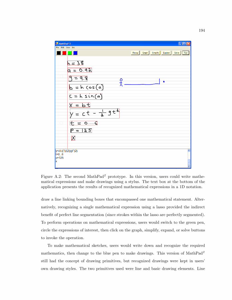
194
Figure A.2: The second MathPad2 prototype. In this version, users could write mathe-matical expressions and make drawings using a stylus. The text box at the bottom of theapplication presents the results of recognized mathematical expressions in a 1D notation.
draw a line linking bounding boxes that encompassed one mathematical statement. Alter-
natively, recognizing a single mathematical expression using a lasso provided the indirect
benefit of perfect line segmentation (since strokes within the lasso are perfectly segmented).
To perform operations on mathematical expressions, users would switch to the green pen,
circle the expressions of interest, then click on the graph, simplify, expand, or solve buttons
to invoke the operation.
To make mathematical sketches, users would write down and recognize the required
mathematics, then change to the blue pen to make drawings. This version of MathPad2
still had the concept of drawing primitives, but recognized drawings were kept in users’
own drawing styles. The two primitives used were line and basic drawing elements. Line

195
primitives had the special property that an axis name and length could be associated with
them for labeling and dimensioning coordinates for animation, while basic drawing elements
could have any mathematical expression associated to them and be animated during a sketch
run. To make associations, users lassoed one or more of the mathematical expressions
with the blue pen. Once this lasso was made, the system went into association mode and
drawing elements were highlighted as the pen cursor hovered over them. Users completed
the association by tapping on the highlighted element. In Figure A.2, users would lasso all
but the final two expressions and associate them with the ball. The final two expressions,
which are used for defining the coordinate system, would be associated with the horizontal
line; users would then click the run button to see the animation. Finally, users could also
modify existing expressions, recognize them again, and rerun the animation to see the effects
of any changes without having to reassociate the mathematics to the drawing elements.
The major lesson learned from the second MathPad2 prototype was that the Ink Divider
object was too unreliable in segmenting to use consistently. Although the ability simply
to click on the recognition button to recognize all of the written mathematics is useful,
the lasso technique for recognition is obviously more reliable, with the tradeoff of having
to perform the operation for every expression. Additionally, we realized that a number of
features were missing from the user interface. First, graphing, simplification, expansion,
and solving tools needed a better invocation method. Second, we needed to allow users to
specify composite objects. Third, we wanted to give users more functionality in what they
could draw by letting them create non-rigid objects. Fourth, we wanted to expand what
mathematical sketching could do by allowing rotations.
A.3 Prototype Three
The third prototype’s main focus was to make functional additions to the second prototype
and to use more gestural interaction in the interface (Figure A.3). For example, we replaced
the need to click on the graph, simplify, expand, and solve buttons with a gestural interface
to invoke these tasks (we also added the ability to do factoring). To invoke a graph wid-
get, users simply had to draw a sufficiently long line from the mathematical expression to
anywhere on the paper. To solve equations, users made a squiggle gesture with two loops

196
Figure A.3: The third MathPad2 prototype. In this version, users could specify rotations,make composite objects, nail drawing elements to one another, and use a gestural interfaceto invoke graphing and other operations.
starting inside the mathematical expression’s bounding box. For simplification, expansion,
and factoring, users would write an equal sign to the right of an expression, then draw a
dot, horizontal line, or vertical line respectively.
To handle composite drawing objects, we chose to have users simply lasso the individual
strokes. The drawback of this approach was that we could not use the black or blue pen to
do this, since black-pen lassoing was used for recognition and blue-pen lassoing was used for
making associations. We thus added a new mode to the system: users would switch to the
magenta pen to make associations and create composite drawing elements. This also freed
the blue pen for making drawings that might have been misinterpreted as a lasso (e.g., a
smiley face with the face drawn first).
197
To let drawing elements rotate, users needed to specify a rotation point. Using the
magenta pen as the association pen, we extended the association mode’s interface by letting
users make a rotation point whenever they made an association. So, instead of simply
tapping on a drawing element to complete an association, users could make a gesture whose
initial point determined what drawing element was associated with the lassoed expressions,
and whose last point would specify the rotation point. Finally, to provide more drawing
flexibility, we wanted to let users make non-rigid objects. Using a nail-based approach,
users could draw a small circle with the magenta pen around one or more drawing elements.
MathPad2 would then recognize the circle and nail the drawing elements together at the
given location (the circle’s center point). During animation, an object nailed in two locations
would stretch if it was attached to a moving object.
With the implementation of the third MathPad2 prototype, we realized that three im-
portant changes were needed to improve the system and mathematical sketching in general.
First, as we added more functionality to the system, more modes were needed. We wanted
a modeless user interface so users would not have to switch continuously among black, blue,
and magenta pens. Second, after looking at a number of physics and math textbooks, it
became clear that diagrams and illustrations are almost always labeled to identify individ-
ual drawing elements. Therefore, in MathPad2 , it made sense to infer associations from
the labels users place next to a drawing. Third, viewing 1D notation to see if a recognized
mathematical expression is correct can be tedious, especially for complex mathematical
expressions. We thus wanted to remove the recognition text box and let the recognized
mathematics be expressed “in place” (where users wrote them) and in their own handwrit-
ing.

Appendix B
Subject Questionnaires
This appendix shows the questionnaires given to the subjects of the MathPad2 usability
study.
B.1 Pre-Questionnaire
Age:
Sex: M or F
Handedness: Left or Right
Have you ever used a pen-based computer? Yes or No
Have you ever used mathematical software (e.g., Matlab, Mathematica)? Yes or No
If so, which ones?
198

199
B.2 Post-Questionnaire
Overall Reaction to MathPad2
Please rate your overall reaction to MathPad2
Terrible 1 2 3 4 5 6 7 Wonderful
Difficult 1 2 3 4 5 6 7 Easy
Frustrating 1 2 3 4 5 6 7 Satisfying
Dull 1 2 3 4 5 6 7 Stimulating
Why did you choose these ratings?
MathPad2 ’s User Interface
Writing Math Easy 1 2 3 4 5 6 7 Hard
Recognizing Math Expressions Easy 1 2 3 4 5 6 7 Hard
Making Graphs Easy 1 2 3 4 5 6 7 Hard
Solving Equations Easy 1 2 3 4 5 6 7 Hard
Evaluating Expressions Easy 1 2 3 4 5 6 7 Hard
Grouping Drawing Elements Easy 1 2 3 4 5 6 7 Hard
Making Associations Easy 1 2 3 4 5 6 7 Hard
Making Nails Easy 1 2 3 4 5 6 7 Hard
Which method of making associations did you prefer and why?
Did the correction user interface help in fixing recognition mistakes? Yes or No
If not, why not? Is there any improvement you think would make the correction user inter-
face better?
List the most positive aspects of the user interface.
List the most negative aspects of the user interface.

200
Overall, please rate MathPad2 ’s ease of use.
Easy 1 2 3 4 5 6 7 Hard
Please explain your answer.
Recall Test — What Gestures Would You Use?
How would you graph the following expression?
How would you solve the following equation?
How would you evaluate the following expression?
How would you recognize the following expression?
How would you nail the spring to the box?
How would you associate the following number to the line?

201
Perceived Usefulness
Using MathPad2 in my work would enable me to accomplish tasks more quickly.
Unlikely 1 2 3 4 5 6 7 Likely
Using MathPad2 would improve my performance.
Unlikely 1 2 3 4 5 6 7 Likely
Using MathPad2 in my work would increase my productivity.
Unlikely 1 2 3 4 5 6 7 Likely
Using MathPad2 would enhance my effectiveness in my work.
Unlikely 1 2 3 4 5 6 7 Likely
Using MathPad2 would make it easier to do my work.
Unlikely 1 2 3 4 5 6 7 Likely
I would find MathPad2 useful in my work.
Unlikely 1 2 3 4 5 6 7 Likely
Please explain your ratings.
Is there anything you would like to see MathPad2 do that it currently does not support?

Appendix C
Mathematical Expressions Used in
Recognition Experiments
All subjects participating in the mathematical symbol and expression recognition study
(described in Chapter 10) wrote the following 36 mathematical expressions as test data.
The number of symbols and parsing decisions for each expression is also provided.
Mathematical Expression Symbols Parsing Decisions
(ab)x = axbx 10 5
ax
ay = ax−y 10 10
y3 + 3py + q = 0 10 4
y = x + b4a 8 4
a2 + b2 = (a + bc)(a− bc) 17 7
a2 − b2 = (a− b)(a + b) 15 6
2xx2−1
= 1x−1 + 1
x+1 19 20
x = −b+√
b2−4ac2a 15 24
ax4 + bx3 + cx2 + dx + e = 0 18 10
a4 + b4 = (a2 +√
2ab + b2)(a2 −√
2ab + b2) 30 17
(a + b + c)2 = a2 + b2 + 2ab + 2ac + 2bc 26 10
rx = 16a2bc+256a3e−3b4−64a2bd256a5 33 53
202

203
Mathematical Expression Symbols Parsing Decisions
y2 +√
u− p(
y − q2gx
)
+ 2uw = 0 22 20
sin(t) = −4sin3(t) + 3sin(t) 24 3
tan2(x) = 1−cos(2x)1+cos(2x) 27 22
cos(
a2
)
=
√
s(s−a)bc 19 23
a1 + a2 = b3 + c4 + d2 14 8
tan(3a) = −tan3(a)+3tan(a)−3tan2(a)+1
36 33
sin4(h) = 18(3− 4cos(2h) + cos(4h)) 31 8
log(ex) = x 9 1
tan(x−y
2
)
= x−yx+y tan
(
b+c2
)
28 20
px(t) = sin(t−a)sin(t−b)sin(t−c)sin(t) 38 35
py(t) = 1(t−m)2
+ 1(t+n)2
23 19
xx0
+ yy0
= 1 11 10
(g2 + d2)2 = u2(g2 − d2) 16 9
2aba+b =
√
ab(
1− c2
(a+b)2
)
24 39
r2 = (x− x0)2 + (y − y0)
2 + (z − z0)2 27 15
∫
e−xdx = e−x 10 7∫ t0 x2cos(x)dx 13 16∫ 42 y2 − x2dx 10 15
∫ ∫
xy2 + x2ydxdy 13 27
g = 9.8 5 1∫
eax
b+ceaxdx = 1ac log(b + ceax) 29 41
∫
(a + bx)ndx = (a+bx)n+1
(n+1)b 26 31∑n−1
i=0 (i− 1)2 18 8
y =
t : x < 6 and x > 0
t2 : x > 8
t3 : else
24 22

Bibliography
[Aho et al. 1988] Aho, Alfred, Ravi Sethi, and Jeffrey D. Ullman. Compilers: Principles,
Techniques, and Tools, Addison Wesley Publishing Co., 1988.
[Alvarado 2000] Alvarado, Christine J. A Natural Sketching Environment: Bringing the
Computer into Early Stages of Mechanical Design. Master’s Thesis, Department of
Electrical Engineering and Computer Science, Massachusetts Institute of Technology,
May 2000.
[Anderson 1968] Anderson, Robert H. Syntax-Directed Recognition of Hand-Printed Two-
Dimensional Mathematics. PhD Dissertation, Department of Applied Mathematics,
Harvard University, 1968.
[Bahlmann et al. 2002] Bahlmann, Claus, Bernard Haasdonk, and Hans Burkhardt. On-
Line Handwriting Recognition with Support Vector Machines—A Kernel Approach.
In Proceedings of the Eighth International Workshop on Frontiers in Handwriting
Recognition, 49-54, 2002.
[Baker et al. 1996] Baker, James, Isabel Cruz, Giuseppe Liotta, and Roberto Tamassia.
Algorithm Animation Over the World Wide Web. In Proceedings of the International
Workshop on Advanced Visual Interfaces (AVI ’96), 203-212, 1996.
[Barzel et al. 1996] Barzel, Ronen, John F. Hughes, and Daniel N. Wood. Plausible Motion
Simulation for Computer Graphics Animation. In Proceedings of the Eurographics
Workshop on Computer Animation and Simulation’96, Springer Verlag, 183-197, 1996.
204
205
[Belaid and Haton 1984] Belaid, Abdelwaheb and Jean-Paul Haton. A Syntactic Approach
for Handwritten Formula Recognition. IEEE Transactions on Pattern Analysis and
Machine Intelligence, PAMI-6(1):105-111, January 1984.
[Blostein and Grbavec 1997] Blostein, Dorothea and Ann Grbavec. Recognition of Mathe-
matical Notation. In Handbook on Optical Character Recognition and Document Image
Analysis, eds. P.S.P. Wang and H. Bunke, World Scientific Press, 557-582, 1997.
[Borning 1979] Borning, Alan. ThingLab: A Constraint-Oriented Simulation Laboratory.
PhD Dissertation, Stanford University, 1979.
[Brown and Sedgewick 1984] Brown, Marc H., and Robert Sedgewick. A System for Algo-
rithm Animation. In Proceedings of the 11th Annual Conference on Computer Graph-
ics and Interactive Techniques (SIGGRAPH’84), ACM Press, 177-186, 1984.
[Carlson et al. 1996] Carlson, Paul, Margaret Burnett, and Jonathan Cadiz. A Seamless
Integration of Algorithm Animation Into a Visual Programming Language. In Pro-
ceedings of the Workshop on Advanced Visual Interfaces (AVI’96), 194-202, 1996.
[Chan and Yeung 1998a] Chan, Kam-Fai and Dit-Yan Yeung. Elastic Structural Matching
for On-Line Handwritten Alphanumeric Character Recognition. In Proceedings of the
Fourteenth International Conference on Pattern Recognition, 1508-1511, 1998.
[Chan and Yeung 1998b] Chan, Kam-Fai and Dit-Yan Yeung. A Efficient Syntactic Ap-
proach to Structural Analysis of On-Line Handwritten Mathematical Expressions.
Technical Report HKUST-CS98-10, Department of Computer Science, The Hong
Kong University of Science and Technology, Hong Kong, China, August 1998.
[Chan and Yeung 2000a] Chan, Kam-Fai and Dit-Yan Yeung. An Efficient Syntactic Ap-
proach to Structural Analysis of On-Line Handwritten Mathematical Expressions.
Pattern Recognition, 33(3):375-384, March 2000.
[Chan and Yeung 2000b] Chan, Kam-Fai and Dit-Yan Yeung. Mathematical Expression
Recognition: A Survey. International Journal on Document Analysis and Recogni-
tion, 3(1):3-15, 2000.

206
[Chan and Yeung 2001a] Chan, Kam-Fai and Dit-Yan Yeung. PenCalc: A Novel Applica-
tion of On-Line Mathematical Expression Recognition Technology. In Proceedings of
the Sixth International Conference on Document Analysis and Recognition, 774-778,
September 2001.
[Chan and Yeung 2001b] Chan, Kam-Fai and Dit-Yan Yeung. Error Detection, Error Cor-
rection, and Performance Evaluation in On-Line Mathematical Expression Recogni-
tion. Pattern Recognition, 34(8):1671-1684, August 2001.
[Chang 1970] Chang, Shi-Kuo. A Method for the Structural Analysis of Two-Dimensional
Mathematical Expressions. Information Sciences, 2(3):253-272, 1970.
[Chou 1989] Chou, P. Recognition of Equations Using a Two-Dimensional Stochastic
Context-Free Grammar. In Proceedings of SPIE Visual Communications and Image
Processing IV, 852-863, 1989.
[Chin et al. 1988] Chin, John P., Virginia A. Diehl, and Kent L. Norman. Development
of an Instrument Measuring User Satisfaction of the Human-Computer Interface.
In Proceedings of the ACM Conference on Human Factors and Computing Systems
(CHI’88), ACM Press, 213-218, 1988.
[Christian and Titus 1998] Christian, Wolfgang and Aaron Titus. Developing Web-Based
Curricula Using Java Physlets. Computers in Physics, 12(3):227-232, May-June 1998.
[Connell and Jain 2000] Connell, Scott D. and Anil K. Jain. Template-Based On-Line Char-
acter Recognition. Pattern Recognition, 34(1):1-14, January 2000.
[Damm et al. 2000] Damm, Christian H., Klaus M. Hansen, and Michael Thomsen. Tool
Support for Cooperative Object-Oriented Design: Gesture-Based Modeling on an
Electronic Whiteboard. In Proceedings of the 2000 SIGCHI Conference on Human
Factors in Computing Systems, ACM Press, 518-525, 2000.
[Davis 1989] Davis, Fred D. Perceived Usefulness, Perceived Ease of Use, and User Accep-
tance of Information Technology. MIS Quarterly, 13(3):319-340, September 1989.

207
[Davis et al. 2003] Davis, James, Maneesh Agrawala, Erika Chuang, Zoran Popovic, and
David Salesin. A Sketching Interface for Articulated Figure Animation. In Proceedings
of the Eurographic/SIGGRAPH Symposium on Computer Animation, 320-328, 2003.
[Davis and Landay 2004] Davis, Richard C. and James A. Landay. Informal Animation
Sketching: Requirements and Design. In Proceedings of AAAI 2004 Fall Symposium
on Making Pen-Based Interaction Intelligent and Natural, Washington, D.C., October
21-24, 2004.
[Dimitriadis and Coronado 1995] Dimitriadis, Yannis A. and Juan Lopez Coronado. To-
wards An Art-Based Mathematical Editor That Uses On-Line Handwritten Symbol
Recognition. Pattern Recognition, 28(6):807-822, 1995.
[Day et al. 1972] Day, A. M., J. R. Parks, and P. J. Pobgee. On-Line Written Input to
Computers. Machine Perception of Pictures and Patterns, 233-240, 1972.
[Donahey 1976] Donahey, Alvin V. Character Recognition System and Method. United
States Patent 3,996,557, 1976.
[Duda et al. 2001] Duda, Richard O., Peter E. Hart, and David G. Stork. Pattern Classifi-
cation, John Wiley and Sons, 2001.
[Fateman et al. 1996] Fateman, Richard J., Taku Tokuyasu, Benjamin P. Berman, and
Nicholas Mitchell. Optical Character Recognition and Parsing of Typeset Mathemat-
ics. Journal of Visual Communication and Image Representation, 7(1):2-15, 1996.
[Faure and Wang 1990] Faure, Claudie and Zi Xiong Wang. Automatic Perception of the
Structure of Handwritten Mathematical Expressions. In Computer Processing of
Handwriting, eds. R. Plamondon, C. G. Leedham, World Scientific Publishing Com-
pany, 337-361, 1990.
[Feiner et al. 1982] Feiner, Steven, David Salesin, and Thomas Banchoff. Dial: A Diagram-
matic Animation Language. IEEE Computer Graphics and Applications, 2(7):43-54,
1982.

208
[Fukuda et al. 1999] Fukuda, Ryoji, Sou I, Fumikazu Tamari, Xie Ming, and Masakazu
Suzuki. A Technique of Mathematical Expression Structure Analysis for the Hand-
writing Input System. In Proceedings of the Fifth International Conference on Docu-
ment Analysis and Recognition, IEEE Press, 131-134, 1999.
[Ford 1992] Ford, Lewis A. Student Solutions Manual to Accompany University Physics.
Addison-Wesley, 1992.
[Forsberg et al. 1998] Forsberg, Andrew, Mark Dieterich, and Robert Zeleznik. The Music
Notepad. Proceedings of the 11th Annual ACM Symposium on User Interface Software
and Technology, ACM Press, 203-210, 1998.
[Freund and Schapire 1997] Freund, Yoav, and Robert E. Schapire. A Decision-Theoretic
Generalization of On-Line Learning and an Application to Boosting. Journal of Com-
puter and System Sciences, 55(1):119-139, August 1997.
[Garain and Chaudhuri 2004] Garain, Utpal, and B. B. Chaudhuri. Recognition of Online
Handwritten Mathematical Expressions. IEEE Transactions on Systems, Man, and
Cybernetics—Part B: Cybernetics, 34(6):2366-2376, December 2004.
[Giraud-Carrier 2000] Giraud-Carrier, Christophe. A Note on the Utility of Incremental
Learning. AI Communications, 13(4):215-223, December 2000.
[Grbavec and Blostein 1995] Grbavec, Ann, and Dorothea Blostein. Mathematics Recogni-
tion Using Graph Rewriting. In Third International Conference on Document Analysis
and Recognition, 417-421, 1995.
[Groner 1968] Groner, G. F. Real-Time Recognition of Hand-printed Symbols. Pattern
Recognition, ed. L.N. Kanal, 103-108, 1968.
[Gross and Do 1996] Gross, Mark D., and Ellen Yi-Luen Do. Ambiguous Intentions: A
Paper-Like Interface for Creative Design. In Proceedings of the 9th Annual ACM
Symposium on User Interface Software and Technology, ACM Press, 183-192, 1996.
[Gross 1994] Gross, Mark D. Sketch-a-Sketch: A Dynamic Diagrammer. In Proceedings of
the IEEE Symposium on Visual Languages, IEEE Press, 232-238, 1994.

209
[Guerfali and Plamondon 1993] Guerfali, Wacef and Rejean Plamondon. Normalizing and
Restoring On-Line Handwriting. Pattern Recognition, 26(3):419-431, March 1993.
[Guimbretiere and Winograd 2000] Guimbretiere, Francois and Terry Winograd. Flow-
Menu: Combining Command, Text, and Data Entry. In Proceedings of the ACM
Symposium on User Interface Software and Technology (UIST 2000), ACM Press,
213-216, 2000.
[Guzdial 2000] Guzdial, Mark J. Squeak: Object-Oriented Design with Multimedia Applica-
tions. Prentice Hall, 2000.
[Ha et al. 1995] Ha, J., R. Haralick, and I. Philips. Recursive X-Y Cut Using Bounding
Boxes of Connected Components. In Proceedings of the Third International Confer-
ence on Document Analysis and Recognition, 952-955, 1995.
[Hanaki and Yamazaki 1980] Hanaki, Shin-Ichi and Takemi Yamazaki. On-Line Recogni-
tion of Hand-printed Kanji Characters. Pattern Recognition, Vol. 12, 421-429, 1980.
[Hansen and Johnson 2005] Hansen, Charles and Christopher Johnson (eds.). The Visual-
ization Handbook, Elsevier Academic Press, 2005.
[Haines 1994] Haines, Eric. Point in Polygon Strategies, In Graphics Gems IV, ed. Paul S.
Heckbert, Academic Press, 24-46, 1994.
[Hecht 2000] Hecht, Eugene. Physics: Calculus. Brooks/Cole Publishing Company, 2000.
[Hinckley et al. 2005] Hinckley, Ken, Patrick Baudish, Gonzalo Ramos, and Francois Guim-
bretiere. Design and Analysis of Delimiters for Selection-Action Pen Gesture Phrases
in Scriboli. In Proceedings of the ACM Conference on Human Factors in Computing
Systems (CHI 2005), ACM Press, 2005.
[Ho et al. 1994] Ho, Tin Kam, Jonathan J. Hull, and Sargur N. Srihari. Decision Combi-
nation in Multiple Classifier Systems. IEEE Transactions on Pattern Analysis and
Machine Intelligence, 16(1):66-75, January 1994.

210
[Hull 1996] Hull, Jesse F. Recognition of Mathematics Using a Trainable Context-Free
Grammar. Master’s Thesis, Department of Electrical Engineering and Computer Sci-
ence, Massachusetts Institute of Technology, June 1996.
[Igarashi et al. 1999] Igarashi, Takeo, Satoshi Matsuoka, and Hidehiko Tanaka. Teddy: A
Sketching Interface for 3D Freeform Design. In Proceedings of the 26th Annual Confer-
ence on Computer Graphics and Interactive Techniques, ACM Press/Addison-Wesley,
409-416, 1999.
[Igarashi and Hughes 2001] Igarashi, Takeo, and John F. Hughes. A Suggestive Interface
for 3D Drawing. In Proceedings of the ACM Symposium On User Interface Software
and Technology (UIST 2001), ACM Press, 173-181, 2001.
[Impedovo et al. 1978] Impedovo, S., B. Marangelli, and A. M. Fanelli. A Fourier Descriptor
Set for Recognizing Nonstylized Numerals. IEEE Transactions on Systems, Man, and
Cybernetics, SMC-8(8):640-645, August 1978.
[Kara et al. 2004] Kara, Levent Burak, Leslie Gennari, and Thomas F. Stahovich. A Sketch-
Based Interface for the Design and Analysis of Simple Vibratory Mechanical Systems.
In Proceedings of ASME International Design Engineering Technical Conferences,
2004.
[Kerrick and Bovik 1988] Kerrick, David D. and Alan C. Bovik. Microprocessor-Based
Recognition of Hand-printed Characters From a Tablet Input. Pattern Recognition,
21(5):525-537, May 1988.
[Kincaid and Cheney 1996] Kincaid, David and Ward Cheney. Numerical Analysis, Second
Edition. Brooks/Cole Publishing Company, 1996.
[Koschinski et al. 1995] Koschinski M., H.-J. Winkler, and M. Lang. Segmentation and
Recognition of Symbols Within Handwritten Mathematical Expressions. In 1995 In-
ternational Conference on Acoustics, Speech, Signal Processing, 2439-2442, 1995.

211
[Kosmala and Rigoll 1998] Kosmala, Andreas and Gerhard Rigoll. On-Line Handwritten
Formula Recognition Using Statistical Methods. In Proceedings of the International
Conference on Pattern Recognition, 1306-1308, 1998.
[LaFollette et al. 2000] LaFollette, Paul, James Korsh, and Raghvinder Sangwan. A Visual
Interface for Effortless Animation of C/C++ Programs. Journal of Visual Languages
and Computing, 11(1):27-48, 2000.
[Kurtenbach and Buxton 1994] Kurtenbach, Gordon and William Buxton. User Learning
and Performance with Marking Menus. In Proceedings of the ACM Conference on
Human Factors in Computing Systems (CHI’94), ACM Press, 258-264, 1994.
[Laleuf and Spalter 2001] Laleuf, Jean R., and Anne Morgan Spalter. A Component Reposi-
tory for Learning Objects: A Progress Report. In Proceedings of the First ACM/IEEE-
CS Joint Conference on Digital Libraries, ACM Press, 33-40, 2001.
[Landay and Myers 1995] Landay, James A., and Brad A. Myers. Interactive Sketching
for the Early Stages of User Interface Design. In Proceedings of the 1995 SIGCHI
Conference on Human Factors in Computing Systems, ACM Press, 43-50, 1995.
[LaViola and Zeleznik 2004] LaViola, Joseph and Robert Zeleznik. MathPad2 : A System
for the Creation and Exploration of Mathematical Sketches. ACM Transactions on
Graphics (Proceedings of SIGGRAPH 2004), 23(3):432-440, August 2004.
[Lavirotte and Pottier 1997] Lavirotte, Stephane and Loic Pottier. Optical Formula Recog-
nition. In Fourth International Conference on Document Analysis and Recognition,
IEEE Press, 357-361, 1997.
[Lee and Wang 1995] Lee, Hsi-Jian and Jiumn-Shine Wang. Design of a Mathematical Ex-
pression Recognition System. In Third International Conference on Document Anal-
ysis and Recognition, IEEE Press, 1084-1087, 1995.
[Lee and Wang 1997] Lee, Hsi-Jian, and Jiumn-Shine Wang. Design of a Mathematical Ex-
pression Recognition System. Pattern Recognition Letters, 18:289-298, 1997.

212
[Lee and Lee 1994] Lee, Hsi-Jian, and Min-Chou Lee. Understanding Mathematical Expres-
sions Using Procedure-Oriented Transformation. Pattern Recognition, 27(3):447-457,
1994.
[Lehmberg et al. 1996] Lehmberg, Stefan, Hans-Jurgen Winkler, and Manfred Lang. A
Soft-Design Approach for Symbol Segmentation Within Handwritten Mathematical
Expressions. In 1996 International Conference on Acoustics, Speech, and Signal Pro-
cessing, 3434-3437, 1996.
[Li and Yeung 1997] Li, Xiaolin, and Dit-Yan Yeung. On-Line Handwritten Alphanu-
meric Character Recognition Using Dominant Points in Strokes. Pattern Recognition,
30(1):31-44, January 1997.
[Lin et al. 2000] Lin, James, Mark W. Newman, Jason I. Hong, and James A. Landay.
DENIM: Finding a Tighter Fit Between Tools and Practice for Web Site Design. CHI
Letters, 2(1):510-517, ACM Press, 2000.
[Littin 1995] Littin, Richard H. Mathematical Expression Recognition: Parsing Pen/Tablet
Input in Real-Time Using LR Techniques. Master’s Thesis, University of Waikato,
Hamilton, New Zealand, 1995.
[Martin 1967] Martin, William J. A Fast Parsing Scheme for Hand-Printed Mathematical
Expressions. Artificial Intelligence Memo No. 145, Massachusetts Institute of Tech-
nology, 1967.
[Marzinkewitsch 1991] Marzinkewitsch, Reiner. Operating Computer Algebra Systems by
Hand-printed Input. In Proceedings of the 1991 International Symposium on Symbolic
and Algebraic Computation, 411-413, 1991.
[Matsakis 1999] Matsakis, Nicholas E. Recognition of Handwritten Mathematical Expres-
sions. Master’s Thesis, Department of Electrical Engineering and Computer Science,
Massachusetts Institute of Technology, 1999.

213
[Miller and Viola 1998] Miller, Erik G., and Paul A. Viola. Ambiguity and Constraint in
Mathematical Expression Recognition. In Proceedings of the Fifteenth National Con-
ference on Artificial Intelligence, 784-791, 1998.
[Moran et al. 1997] Moran, Thomas P., Patrick Chui, and William van Melle. Pen-based
Interaction Techniques for Organizing Material on an Electronic Whiteboard. In Pro-
ceedings of the 10th Annual ACM Symposium on User Interface Software and Tech-
nology, ACM Press, 45-54, 1997.
[Moscovich and Hughes 2004] Moscovich, Tomer, and John F. Hughes. Animation Sketch-
ing: An Approach to Accessible Animation. Technical Report CS-04-03, Computer
Science Department, Brown University, Providence, RI, February 2004.
[Mynatt et al. 1999] Mynatt, Elizabeth D., Takeo Igarashi, W. Keith Edwards, and An-
thony LaMarca. Flatland: New Dimensions in Office Whiteboards. In Proceedings of
the 1999 SIGCHI Conference on Human Factors in Computing Systems, ACM Press,
346-353, 1999.
[Nakayama 1993] Nakayama, Y. A Prototype Pen-Input Mathematical Formula Editor. In
Proceedings of ED-MEDIA 93 — World Conference on Educational Multimedia and
Hypermedia, 400-407, 1993.
[Odaka et al. 1982] Odaka, Kazumi, Hiroki Arakawa, and Isao Masuda. On-Line Recogni-
tion of Handwritten Characters by Approximating Each Stroke with Several Points.
IEEE Transactions on Systems, Man, and Cybernetics, SMC-12(6):898-903, Novem-
ber/December 1982.
[Okamoto and Miao 1991] Okamoto, M. and B. Miao. Recognition of Mathematical Expres-
sions by Using Layout Structures of Symbols. In Proceedings of the First International
Conference on Document Analysis and Recognition, 242-250, 1991.
[Pavlidis et al. 1998] Pavlidis, Ioannis, Rahul Singh, and Nikolaos P. Papanikolopoulos. On-
Line Handwriting Recognition Using Physics-Based Shape Metamorphosis. Pattern
Recognition, 31(11):1589-1600, November 1998.

214
[Pickering et al. 1999] Pickering, Jeff, Dom Bhuphaibool, Joseph LaViola, and Nancy Pol-
lard. The Coach’s Playbook. Technical Report CS-99-08, Brown University, Depart-
ment of Computer Science, Providence, RI, May 1999.
[Plamondon and Maarse 1989] Plamondon, R. and F. J. Maarse. An Evaluation of
Motor Models of Handwriting, IEEE Transactions on Systems, Man, and
Cybernetics,19(5):1060-1072, 1989.
[Plamondon and Srihari 2000] Plamondon, Rejean and Sargur N. Srihari. On-Line and Off-
Line Handwriting Recognition: A Comprehensive Survey. IEEE Transactions on Pat-
tern Analysis and Machine Intelligence, 22(1):63-84, January 2000.
[Powers 1973] Powers, V. M. Pen Direction Sequences in Character Recognition.Pattern
Recognition Vol. 5, 291-302, March 1973.
[Rubine 1991] Rubine, Dean. Specifying Gestures by Example. In Proceedings of SIG-
GRAPH’91, ACM Press, 329-337, 1991.
[Saund et al. 2003] Saund, Eric, David Fleet, Daniel Larner, and James Mahoney.
Perceptually-Supported Image Editing of Text and Graphics. In Proceedings of the
ACM Symposium on User Interface Software and Technology (UIST 2003), ACM
Press, 183-192, 2003.
[Saund and Lank 2003] Saund, Eric, and Edward Lank. Stylus Input and Editing Without
Prior Selection of Mode. In Proceedings of the ACM Symposium on User Interface
Software and Technology (UIST 2003), ACM Press, 213-217, 2003.
[Scattolin and Krzyzak 1994] Scattolin, P. and A. Krzyzak. Weighted Elastic Matching
Method for Recognition of Handwritten Numerals, In Proceedings of Vision Inter-
face’94, 178-185, 1994.
[Schapire 1999] Schapire, Robert. A Brief Introduction to Boosting. In Proceedings of the
16th International Joint Conference on Artificial Intelligence, 1401-1406, 1999.
[Schneider and Eberly 2003] Schneider, Philip J., and David H. Eberly. Geometric Tools
for Computer Graphics, Morgan Kaufmann Publishers, 2003.

215
[Shneiderman 1998] Shneiderman, Ben. Designing the User Interface: Strategies for Effec-
tive Human-Computer Interaction, Third Edition. Addison Wesley Publishing Com-
pany, 1998.
[Smithies et al. 1999] Smithies, Steve, Kevin Novins, and James Arvo. A Handwriting-
Based Equation Editor. In Proceedings of Graphics Interface’99, 84-91, 1999.
[Smithies 1999] Smithies, Steven R. Freehand Formula Entry System. Master’s Thesis, De-
partment of Computer Science, University of Otago, Dunedin, New Zealand, 1999.
[Spalter and Simpson 2000] Spalter, Anne Morgan and Rosemary Michelle Simpson. Inte-
grating Interactive Computer-based Learning Experiences into Established Curricula:
A Case Study. In Proceedings of the 5th Annual SIGCSE/SIGCUE ITiCSE Conference
on Innovation and Technology in Computer Science Education, ACM Press, 116-119,
2000.
[Stasko 1996] Stasko, John T. Using Student-Built Algorithm Animations as Learning Aids.
Graphics, Visualization, and Usability Center, Georgia Institute of Technology, At-
lanta, GA, Technical Report GIT-GVU-96-19, August 1996.
[Stasko 1992] Stasko, John T. Animating Algorithms with XTANGO. SIGACT News,
23(2):67-71, 1992.
[Stasko 1991] Stasko, John T. Using Direct Manipulation to Build Algorithm Animations
by Demonstration. In Proceedings of the ACM Conference on Human Factors and
Computing Systems (CHI’91), ACM Press, 307-314, 1991.
[Tall 1987] Tall, David. Graphical Packages for Mathematics Teaching and Learning. In
Informatics and the Teaching of Mathematics. eds. D.C. Johnson and F. Lovis, North
Holland, 39-47, 1987.
[Tappert et al. 1990] Tappert, Charles C., Ching Y. Seun, and Toru Wakahara. The State
of the Art in On-Line Handwriting Recognition. In IEEE Transactions on Pattern
Analysis and Machine Intelligence, 12(8):787-808, August 1990.

216
[Twaakyodo and Okamoto 1995] Twaakyodo, Hashim M., and Masayuki Okamoto. Struc-
tural Analysis and Recognition of Mathematical Expressions. In Third International
Conference on Document Analysis and Recognition, IEEE Press, 430-437, 1995.
[Varberg and Purcell 1992] Varberg, Dale, and Edwin J. Purcell. Calculus with Analytic
Geometry. Prentice Hall, 1992.
[Vuokko et al. 1999] Vuokko, Vuori, Jorma Laaksonen, Erkki Oja, and Jari Kangas. On-
Line Adaptation in Recognition of Handwritten Alphanumeric Characters. In Pro-
ceedings of the Fifth International Conference on Document Analysis and Recognition,
792-795, 1999.
[Warner et al. 1997] Warner, Simeon, Simon Catterall, and Edward Lipson. Java Simu-
lations for Physics Education. Concurrency: Practice and Experience, 9(6):447-484,
June 1997.
[Wehbi et al. 1995] Wehbi, H., H. Oulhadj, J. Lemoine, and E. Petit. Numerical Characters
and Capital Letters Segmentation Recognition in Mixed Handwriting Context. In
Third International Conference on Document Analysis and Recognition, IEEE Press,
878-881, 1995.
[Weisstein 1998] Weisstein, Eric. CRC Concise Encyclopedia of Mathematics. Chapman and
Hall/CRC, 1998.
[Windows Journal 2005] Windows Journal, Microsoft Corporation, 1981-2005.
[Winkler 1994] Winkler, Hans-Jurgen. Symbol Recognition in Handwritten Mathematical
Formulas. In International Workshop on Modern Modes of Man-Machine Communi-
cation, 7/1-7/10, June 1994.
[Xuejun et al. 1997] Xuejun, Zhao, Lin Xinyu, Zheng Shengling, Pan Baochang, and Yuan
Y. Tang. On-Line Recognition Handwritten Mathematical Symbols. In Fourth Inter-
national Conference on Document Analysis and Recognition, IEEE Press, 645-648,
1997.

217
[Yamazaki 2004] Yamazaki, Kazutoshi. A Multi-Stage Approach to the Recognition and
Parsing of Mathematical Expressions. Master’s Thesis, Department of Computer Sci-
ence, Brown University, May 2004.
[Young 1992] Young, Hugh D. University Physics. Addison-Wesley Publishing Company,
1992.
[Zanibbi et al. 2001a] Zanibbi, Richard, Dorothea Blostein, and James R. Cordy. Baseline
Structure Analysis of Handwritten Mathematics Notation. In Proceedings of the Sixth
International Conference on Document Analysis and Recognition, 768-773, 2001.
[Zanibbi et al. 2001b] Zanibbi, Richard, Kevin Novins, James Arvo, and Katherine Zanibbi.
Aiding Manipulation of Handwritten Mathematical Expressions Through Style-
Preserving Morphs. In Graphics Interface 2001, 127-134, 2001.
[Zanibbi et al. 2002] Zanibbi, Richard, Dorothea Blostein, and James Cordy. Recognizing
Mathematical Expressions Using Tree Transformation. IEEE Transactions on Pattern
Analysis and Machine Intelligence, 24(11):1-13, November 2002.
[Zeleznik et al. 2004] Zeleznik, Robert, Timothy Miller, Loring Holden, and Joseph LaVi-
ola. Fluid Inking: Using Punctuation to Allow Modeless Combination of Marking
and Gesturing. Technical Report CS-04-11, Department of Computer Science, Brown
University, Providence, RI, July 2004.
[Zeleznik et al. 1996] Zeleznik, Robert C., Kenneth P. Herndon, and John F. Hughes.
SKETCH: An Interface for Sketching 3D Scenes. In Proceedings of the 23rd Annual
Conference on Computer Graphics and Interactive Techniques, ACM Press, 163-170,
1996.
[Zhao et al. 1996] Zhao, Y., T. Sakuri, H. Sugiura, and T. Torii. A Methodology of Parsing
Mathematical Notation for Mathematical Computation. In Proceedings of the 1996
International Symposium on Symbolic and Algebraic Computation, 292-300, 1996.