mathematics of climate change
TRANSCRIPT
The Role of Mathematics in Understanding the Earth’s Climate
Andrew Roberts

Outline• What is climate (change)?
• History of mathematics in climate science
• How do we study the climate?
• Dynamical systems
• Large-scale (Atlantic) ocean circulation
• Ice ages and the mid-Pleistocene transition
• Winter is coming?
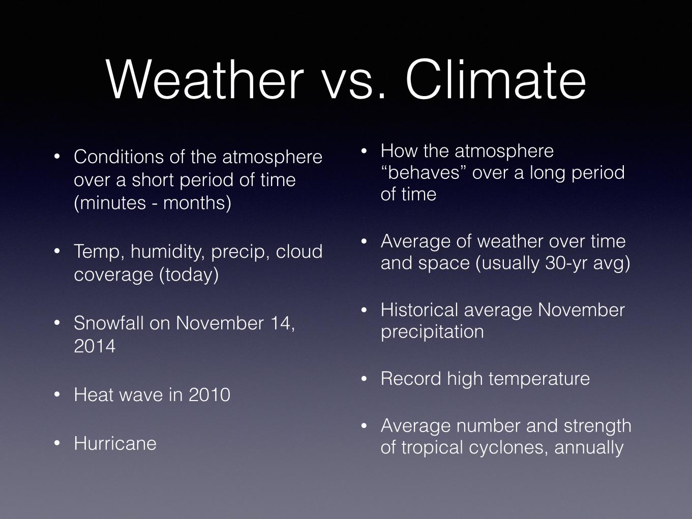
Weather vs. Climate• Conditions of the atmosphere
over a short period of time (minutes - months)
• Temp, humidity, precip, cloud coverage (today)
• Snowfall on November 14, 2014
• Heat wave in 2010
• Hurricane
• How the atmosphere “behaves” over a long period of time
• Average of weather over time and space (usually 30-yr avg)
• Historical average November precipitation
• Record high temperature
• Average number and strength of tropical cyclones, annually
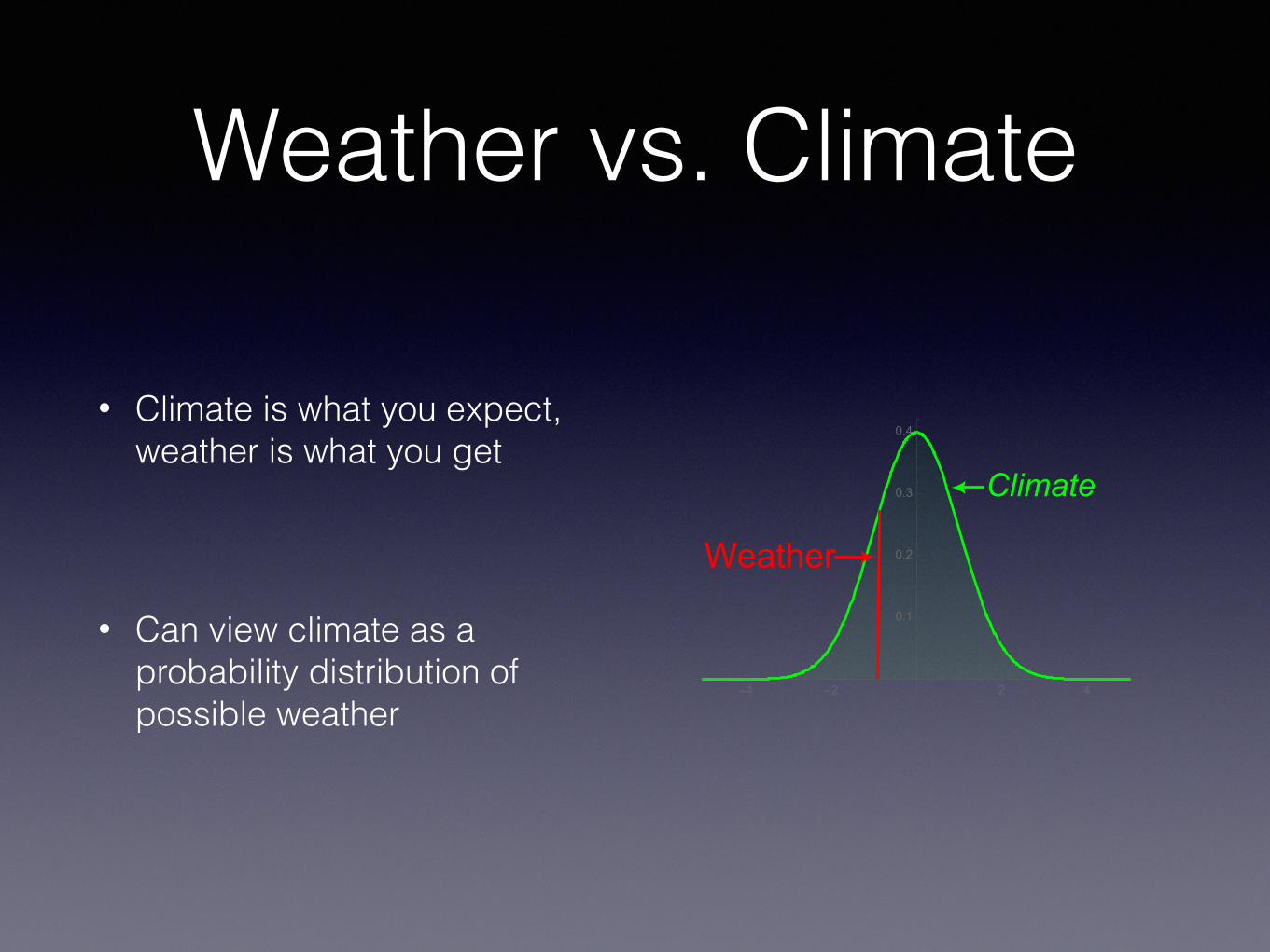
Weather vs. Climate
• Climate is what you expect, weather is what you get
• Can view climate as a probability distribution of possible weather
Climate
Weather
-4 -2 2 4
0.1
0.2
0.3
0.4

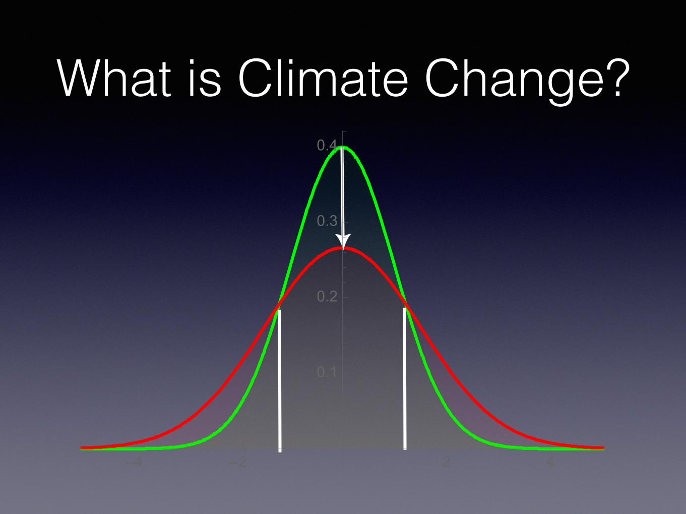
What is Climate Change?
-4 -2 2 4
0.1
0.2
0.3
0.4

What is Climate Change?
-4 -2 2 4
0.1
0.2
0.3
0.4

What is Climate Change?
-4 -2 2 4
0.1
0.2
0.3
0.4
What is Climate Change?
-4 -2 2 4
0.1
0.2
0.3
0.4

PrecipitationDry areas get dryer, wet areas get wetter
Climate scientists predict more floods and
more droughts!

Mathematics and Climate Change
• Energy balance equation
• : incoming solar radiation
• : proportion absorbed by the Earth
• :heat re-radiated back to space
�T = Q(1� ↵(T ))� �T 4
Q
(1� ↵(T ))
�T 4
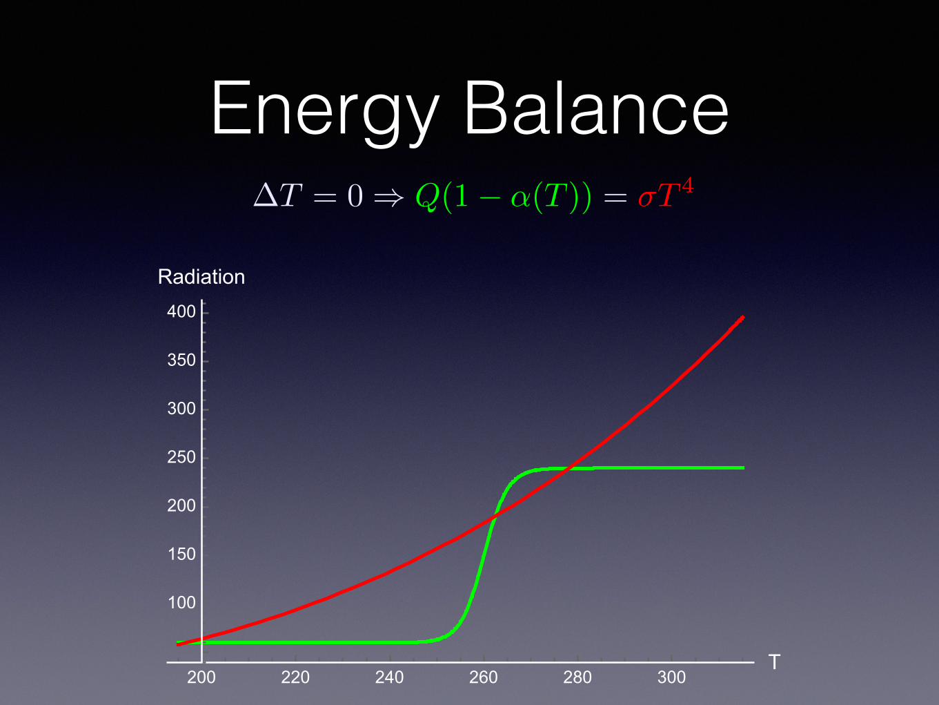
Energy Balance
200 220 240 260 280 300T
100
150
200
250
300
350
400
Radiation
�T = 0 ) Q(1� ↵(T )) = �T 4
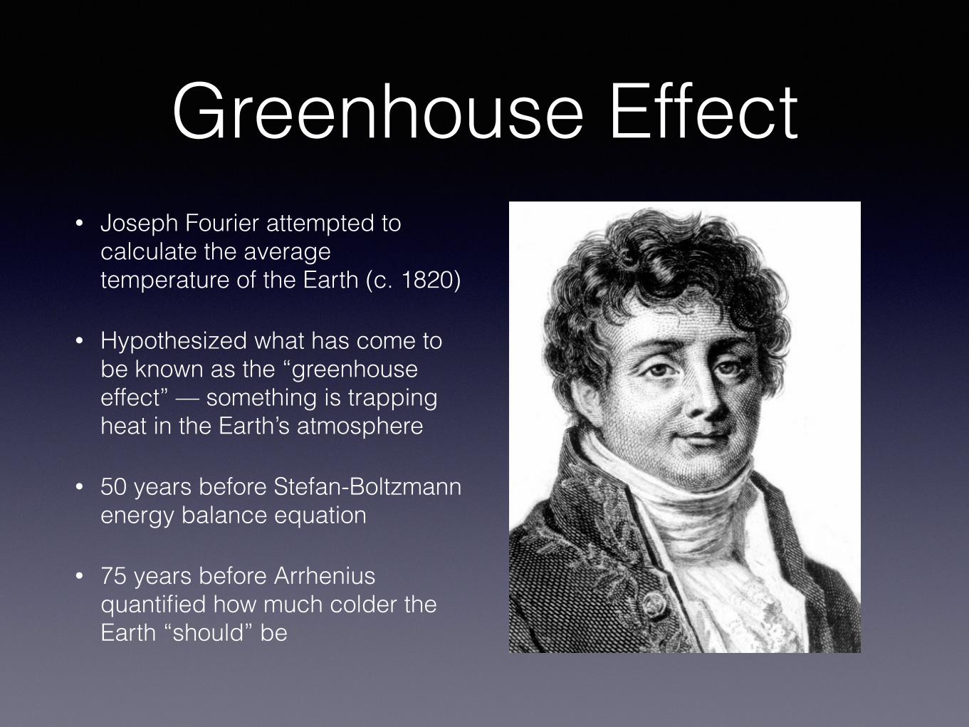
Greenhouse Effect• Joseph Fourier attempted to
calculate the average temperature of the Earth (c. 1820)
• Hypothesized what has come to be known as the “greenhouse effect” — something is trapping heat in the Earth’s atmosphere
• 50 years before Stefan-Boltzmann energy balance equation
• 75 years before Arrhenius quantified how much colder the Earth “should” be

Greenhouse Effect
220 240 260 280 300T
50
100
150
200
250
300
350
400
Radiation
�T = Q(1� ↵(T ))� "�T 4

Energy Balance Cartoon

• Mid-1700s: speculation that ice ages exists
• 1830s: A few geologists claim ice-ages happend, ideas rejected
• 1842: Joseph Adhémar (mathematician) is first to propose ice-ages caused by variation in solar radiation
Ice Ages
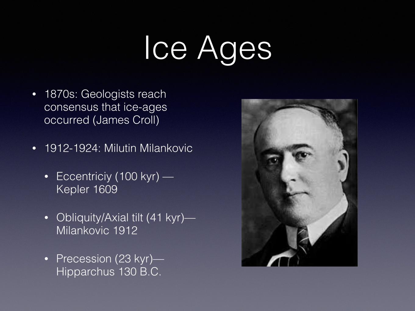
Ice Ages• 1870s: Geologists reach
consensus that ice-ages occurred (James Croll)
• 1912-1924: Milutin Milankovic
• Eccentriciy (100 kyr) —Kepler 1609
• Obliquity/Axial tilt (41 kyr)—Milankovic 1912
• Precession (23 kyr)—Hipparchus 130 B.C.

Milankovic Cycles
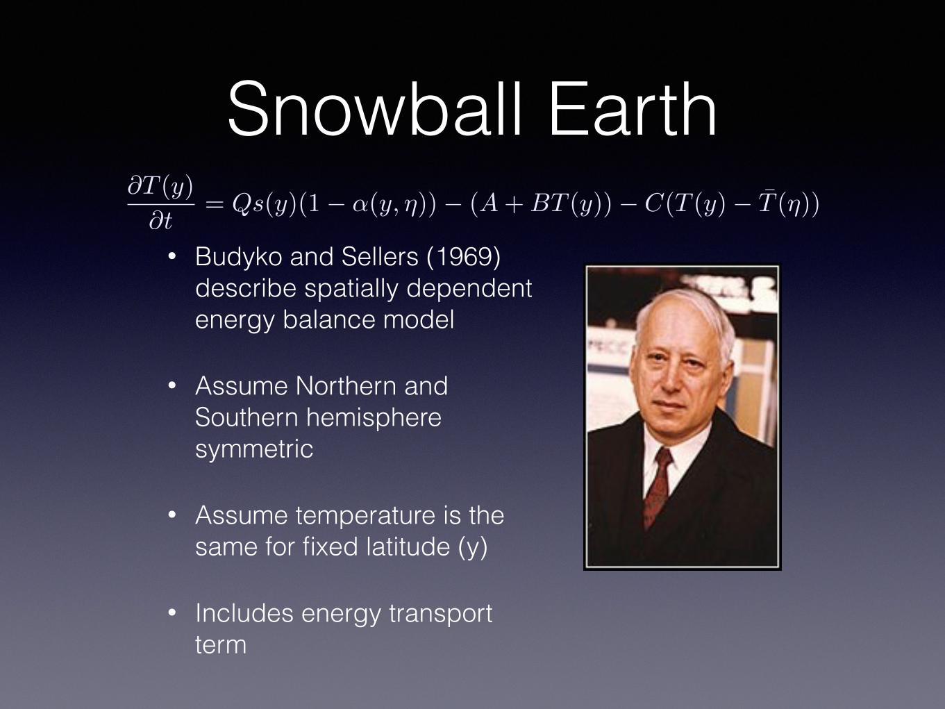
Snowball Earth• Budyko and Sellers (1969)
describe spatially dependent energy balance model
• Assume Northern and Southern hemisphere symmetric
• Assume temperature is the same for fixed latitude (y)
• Includes energy transport term
@T (y)
@t= Qs(y)(1� ↵(y, ⌘))� (A+BT (y))� C(T (y)� T (⌘))
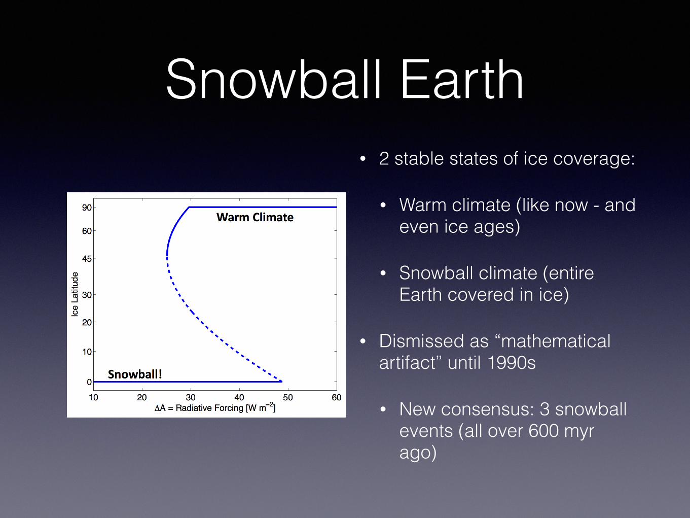
Snowball Earth• 2 stable states of ice coverage:
• Warm climate (like now - and even ice ages)
• Snowball climate (entire Earth covered in ice)
• Dismissed as “mathematical artifact” until 1990s
• New consensus: 3 snowball events (all over 600 myr ago)

How do we study the climate?
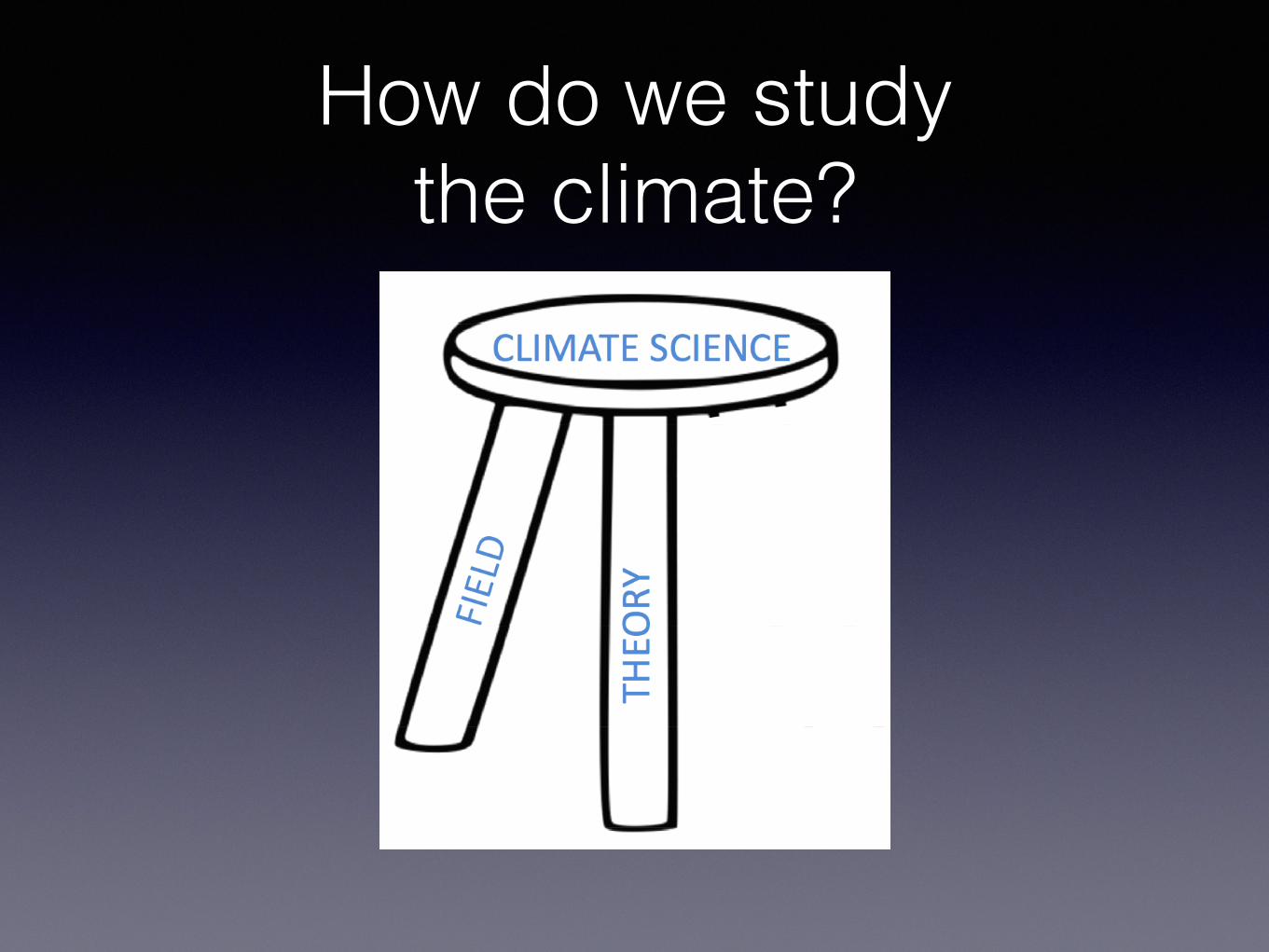
How do we study the climate?

How do we study the climate?
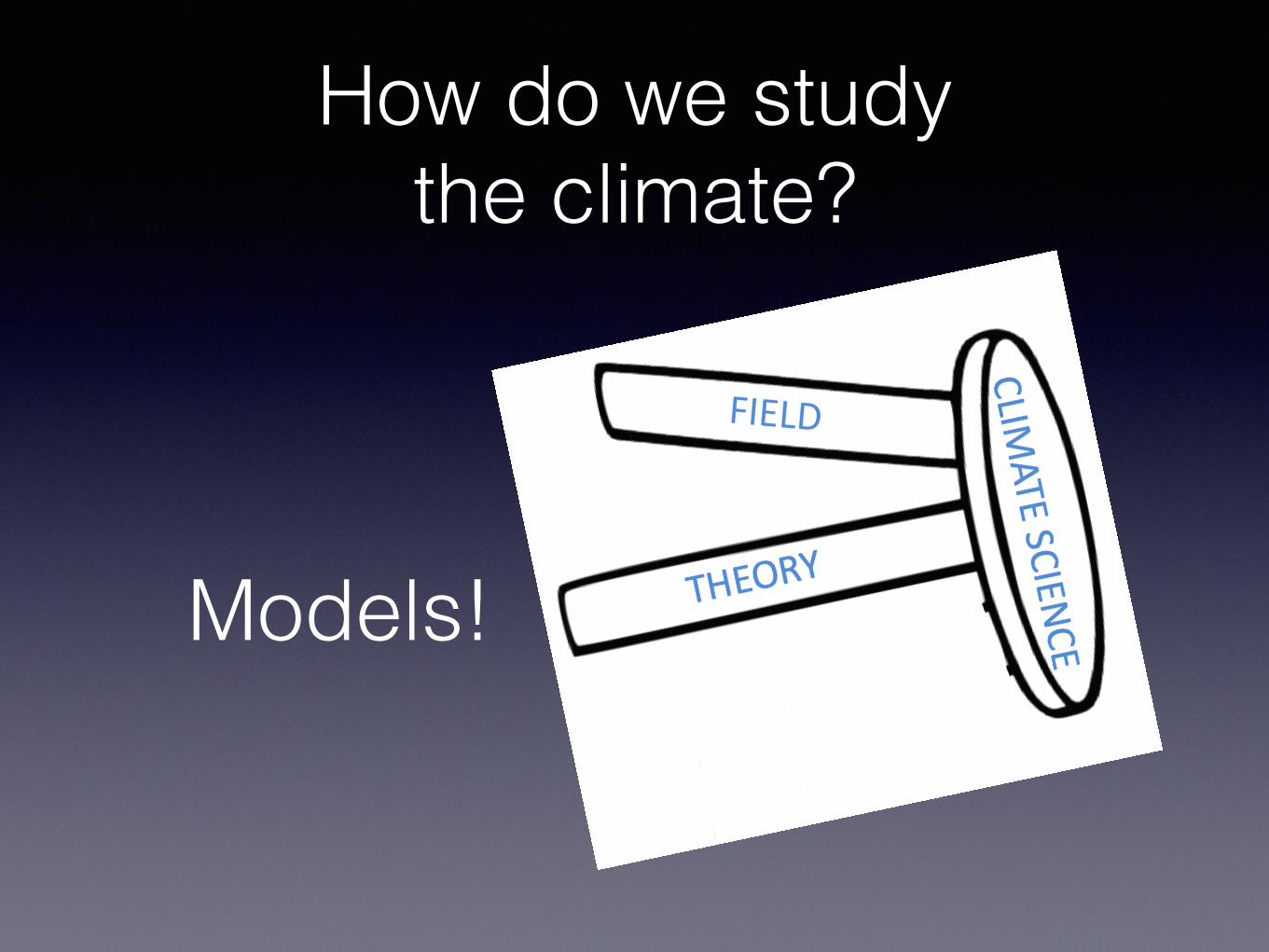
Models!
How do we study the climate?
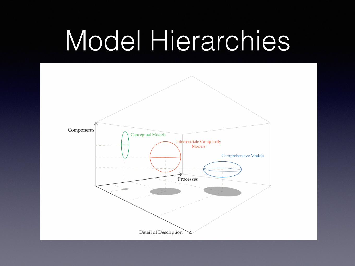
Model Hierarchies
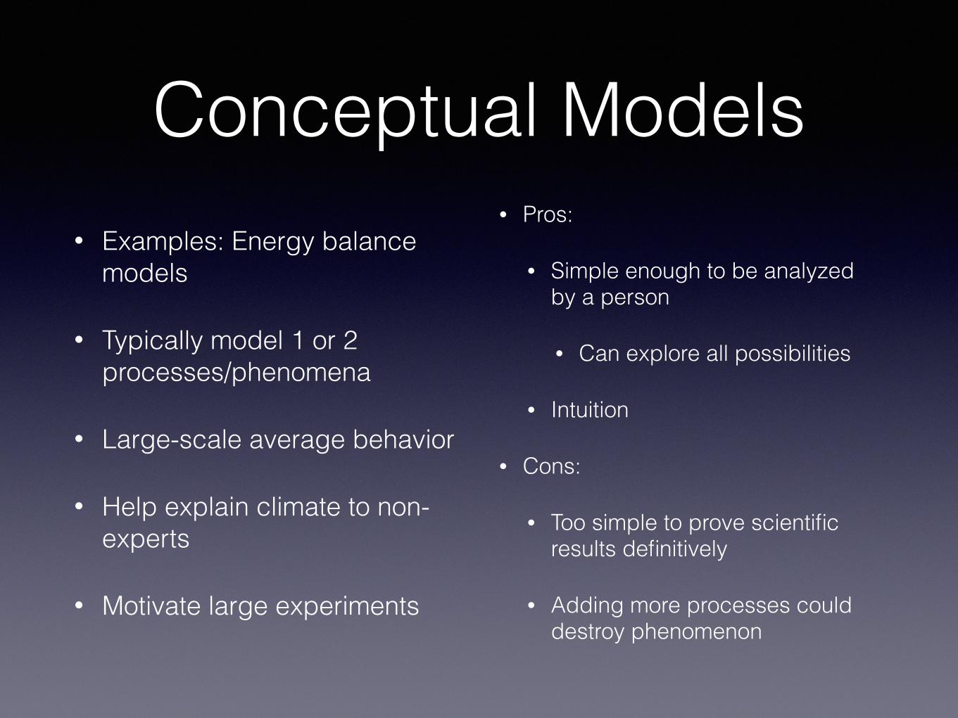
Conceptual Models• Examples: Energy balance
models
• Typically model 1 or 2 processes/phenomena
• Large-scale average behavior
• Help explain climate to non-experts
• Motivate large experiments
• Pros:
• Simple enough to be analyzed by a person
• Can explore all possibilities
• Intuition
• Cons:
• Too simple to prove scientific results definitively
• Adding more processes could destroy phenomenon

Intermediate Complexity and Process Models
• Some spatial resolution
• More processes (but not too many)
• Simple enough for some interpretation
• Too complex to analyze “by hand”
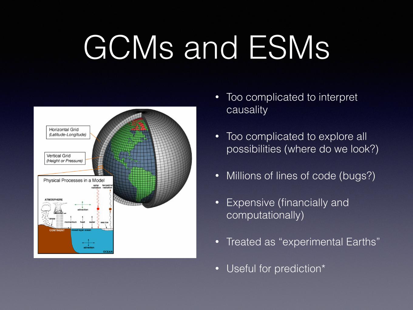
GCMs and ESMs• Too complicated to interpret
causality
• Too complicated to explore all possibilities (where do we look?)
• Millions of lines of code (bugs?)
• Expensive (financially and computationally)
• Treated as “experimental Earths”
• Useful for prediction*

Weather Prediction
Model
Observation of Current State
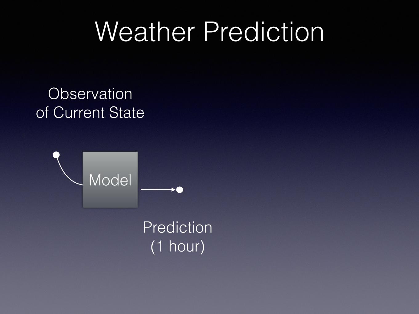
Weather Prediction
Model
Observation of Current State
Prediction (1 hour)

Weather prediction
Model
Observation of Current State
Prediction (1 hour)
Model
Prediction (2 hour)
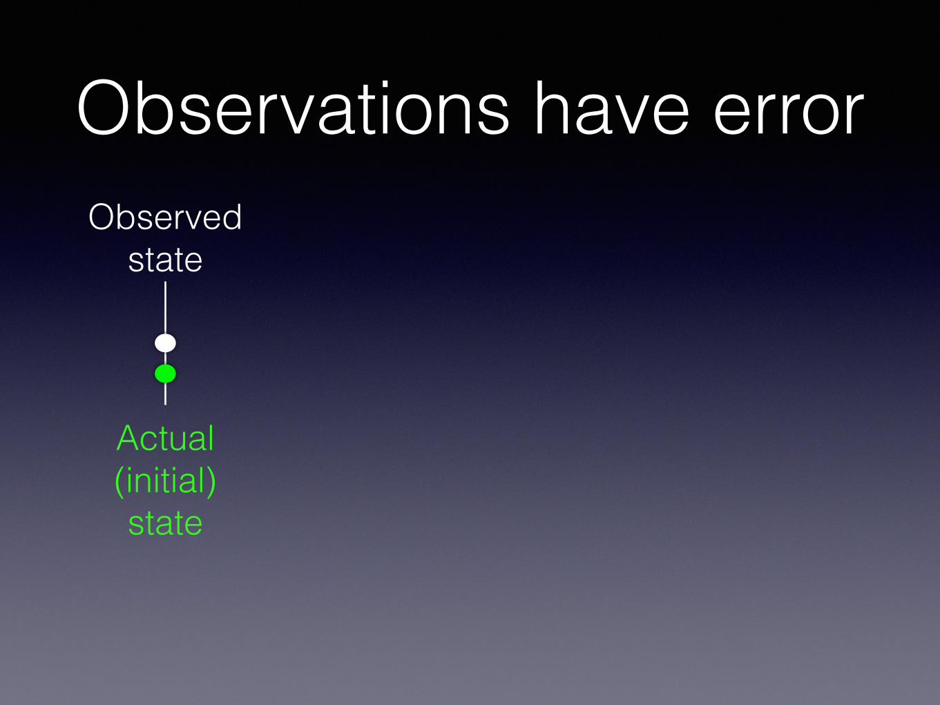
Observations have errorObserved
state
Actual (initial) state
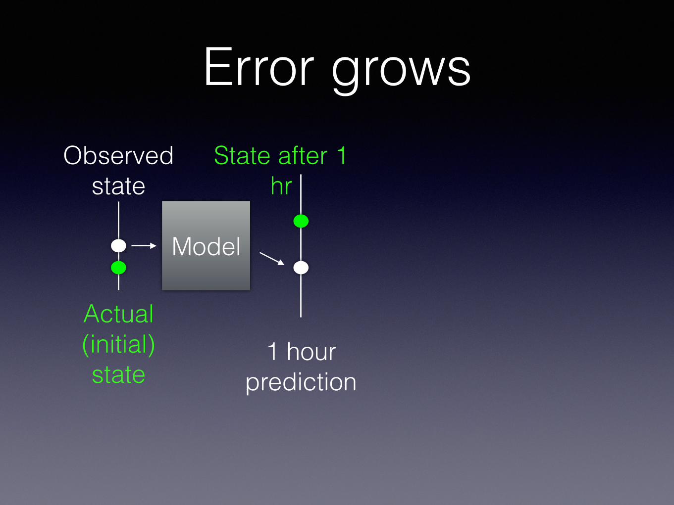
Error grows
Model
Observed state
Actual (initial) state
1 hour prediction
State after 1 hr
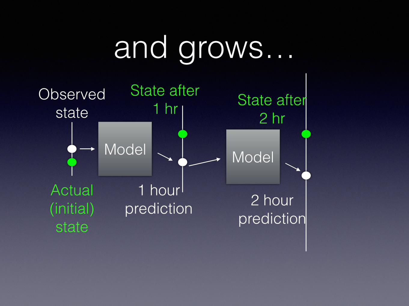
and grows…
Model
Observed state
Actual (initial) state
1 hour prediction
State after 1 hr
Model
2 hour prediction
State after 2 hr
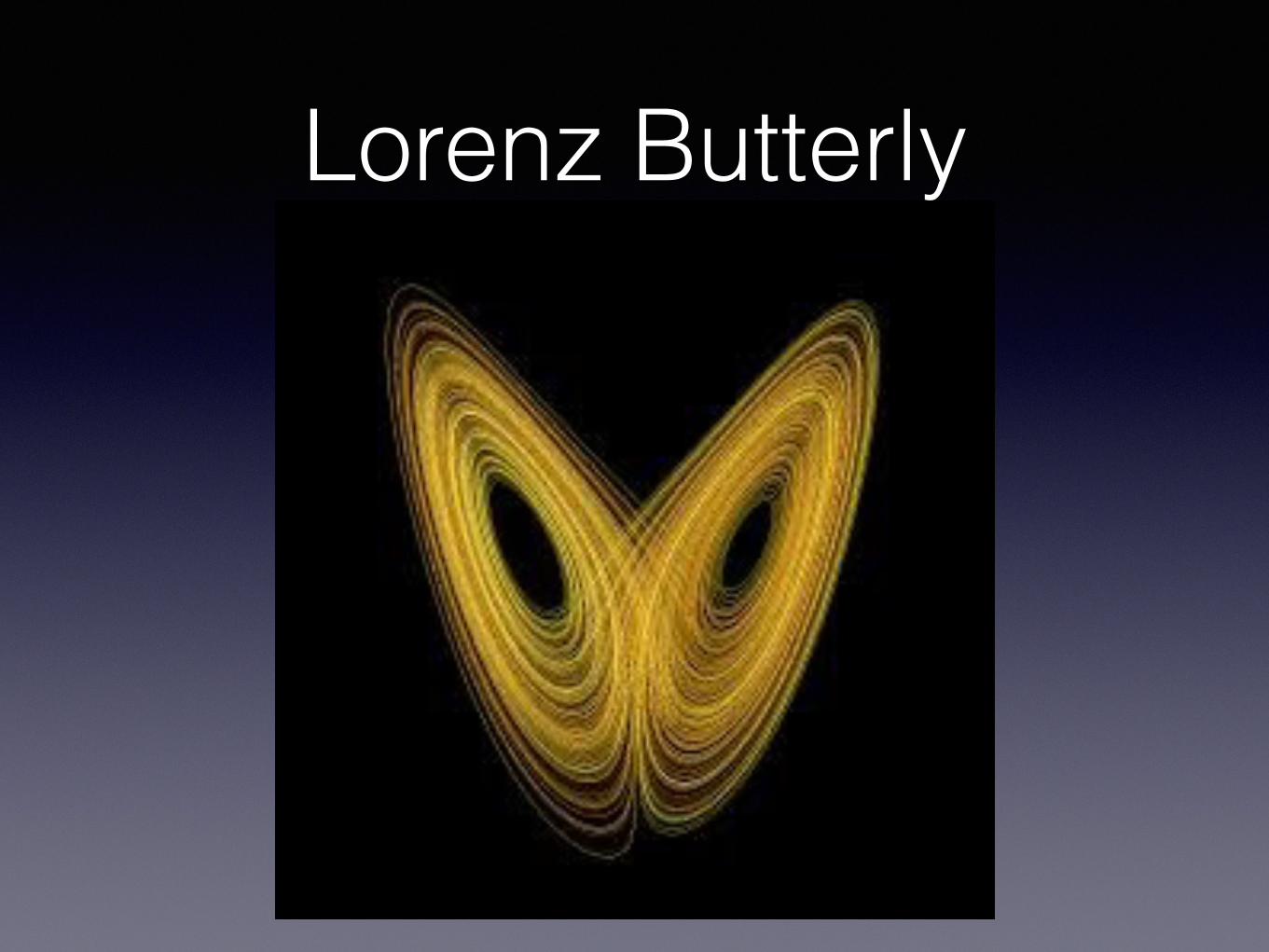
Lorenz Butterly
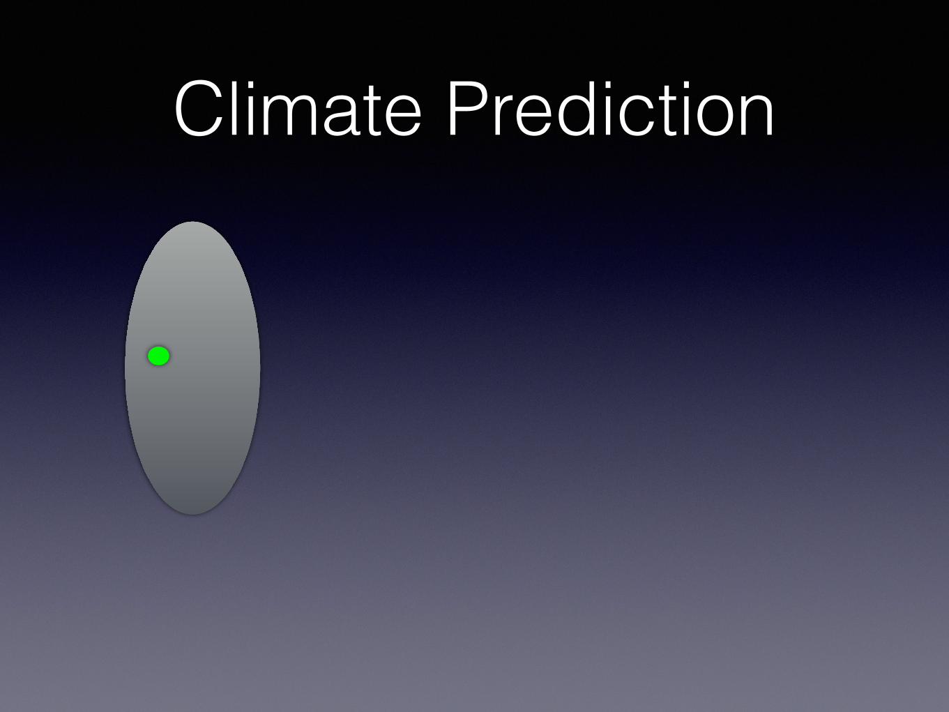
Climate Prediction
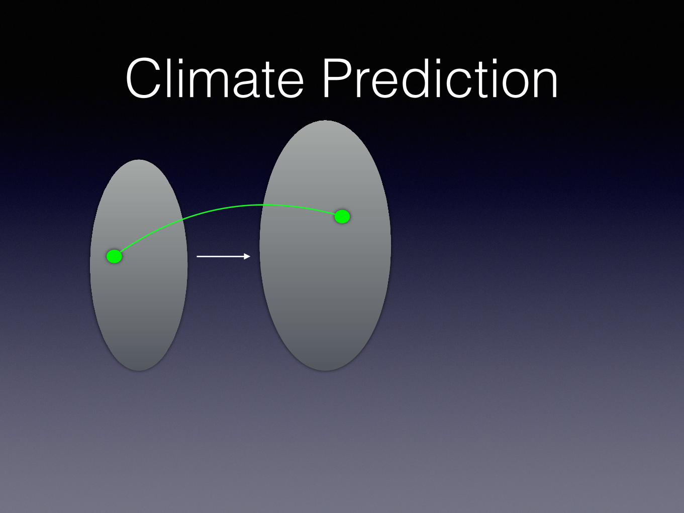
Climate Prediction

Climate Prediction

Climate Prediction
Where do observations come in?

Confronting Models with Data

Confronting Models with Data
1st IC
Model
Data

Confronting Models with Data
1st IC
Model
Data

Data Assimilation
1st IC
Model
Data2nd IC

Data Assimilation
1st IC
Model
Data2nd IC
Model (w/o DA)
Data
Model (w/ DA)

Data Assimilation
1st IC
Model
Data2nd IC
Data
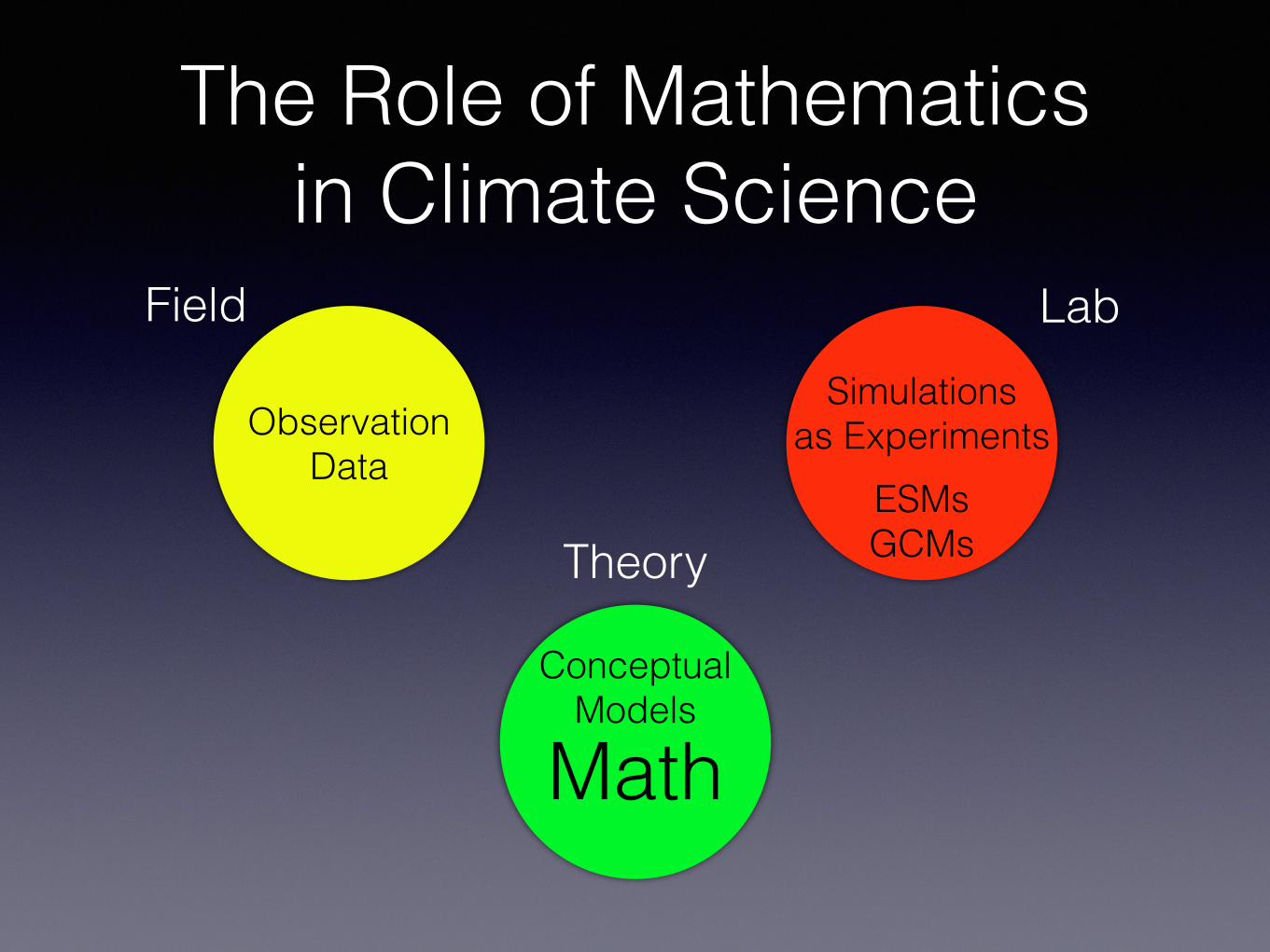
The Role of Mathematics in Climate Science
Observation Data
LabFieldSimulations
as ExperimentsESMs GCMsTheory
Conceptual Models
Math

Dynamical Systems
dx
dt
= f(t)
Derivative (from Calculus)
Example
dx
dt
= t
3 � t+ k
x(t) =t
4
4� t
2
2+ kt+ C

What if dx
dt
= f(x)?
Dynamical Systems
dx
dt
= f(t)
Derivative (from Calculus)
Example
dx
dt
= t
3 � t+ k
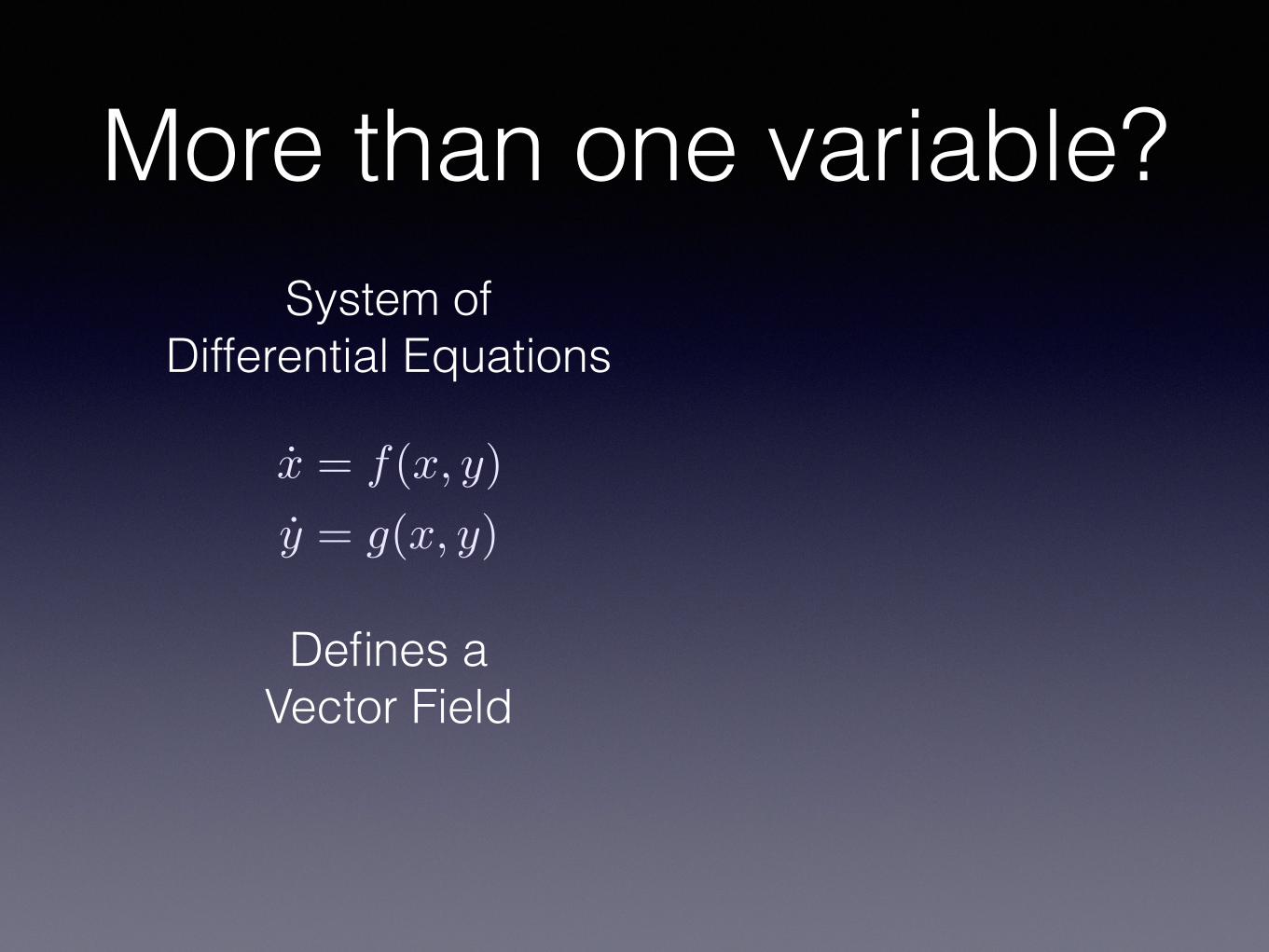
More than one variable?
x = f(x, y)
y = g(x, y)
System of Differential Equations
Defines a Vector Field
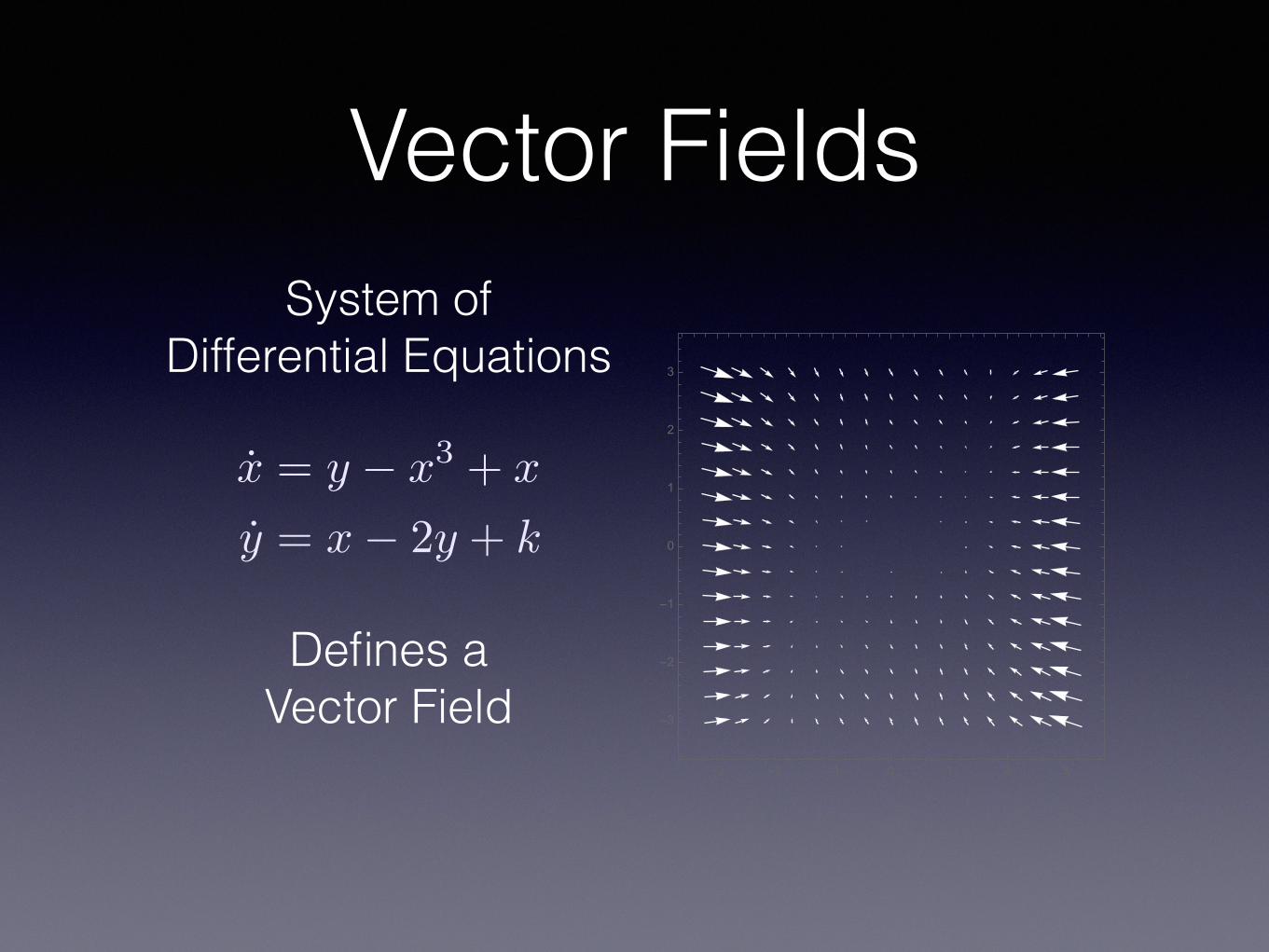
Vector FieldsSystem of
Differential Equations
Defines a Vector Field
x = y � x
3 + x
y = x� 2y + k
-3 -2 -1 0 1 2 3
-3
-2
-1
0
1
2
3

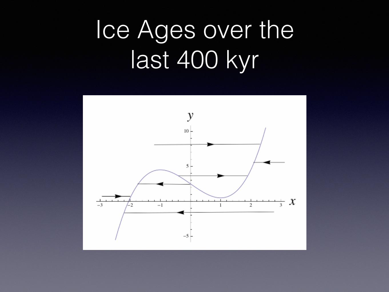
Equilibrium Pointsx = y � x
3 + x
y = x� 2y + k
-3 -2 -1 0 1 2 3
-3
-2
-1
0
1
2
3
Equilibrium points occur when
x = 0
y = 0

Solutionsx = y � x
3 + x
y = x� 2y + k
Even if equations can’t be solved,
we can understand
Qualitative Behavior-3 -2 -1 0 1 2 3
-3
-2
-1
0
1
2
3
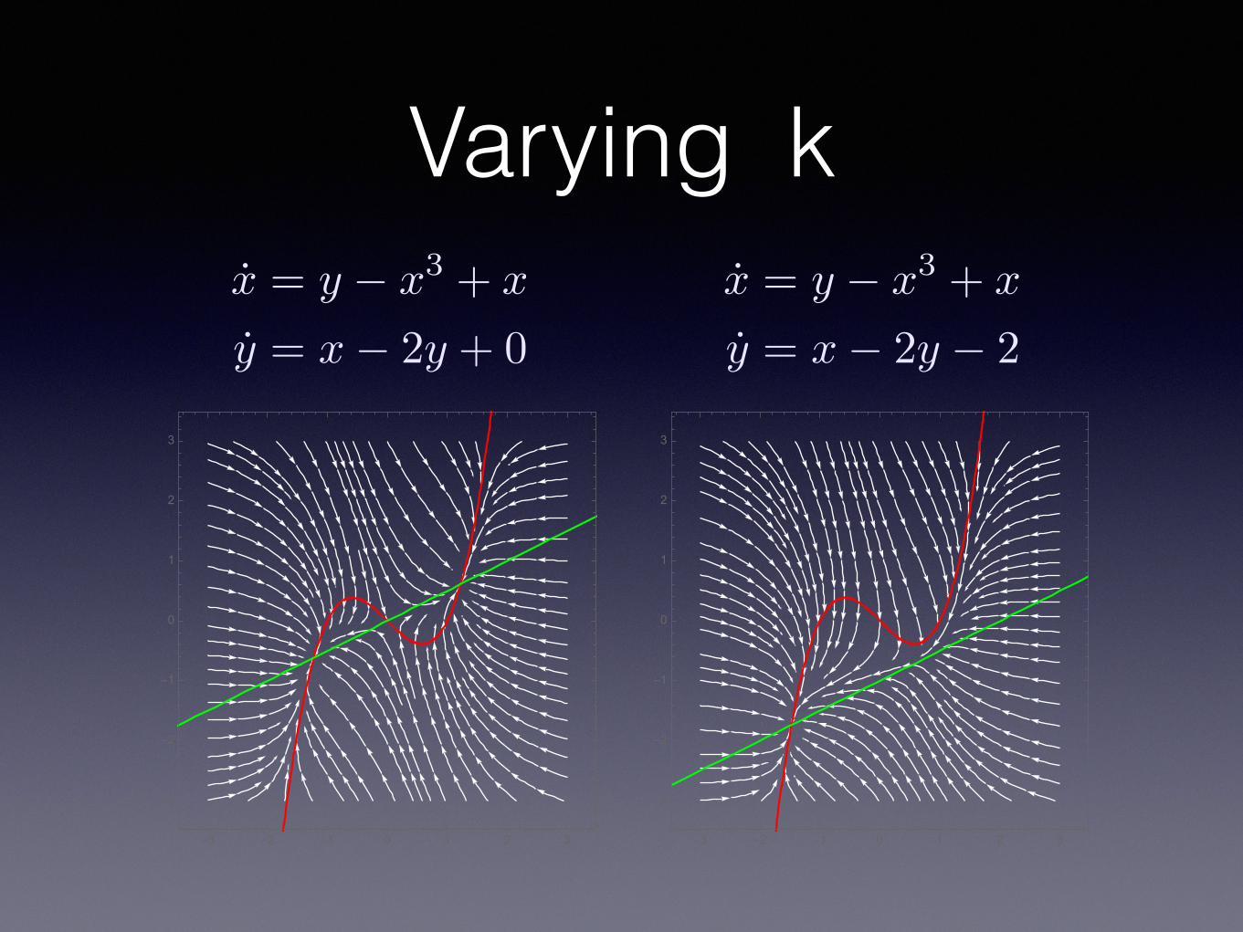
Varying k
-3 -2 -1 0 1 2 3
-3
-2
-1
0
1
2
3
x = y � x
3 + x
y = x� 2y + 0
x = y � x
3 + x
y = x� 2y � 2
-3 -2 -1 0 1 2 3
-3
-2
-1
0
1
2
3

Bifurcation in Algebra I
Quadratic equation
ax
2 + bx+ c = 0
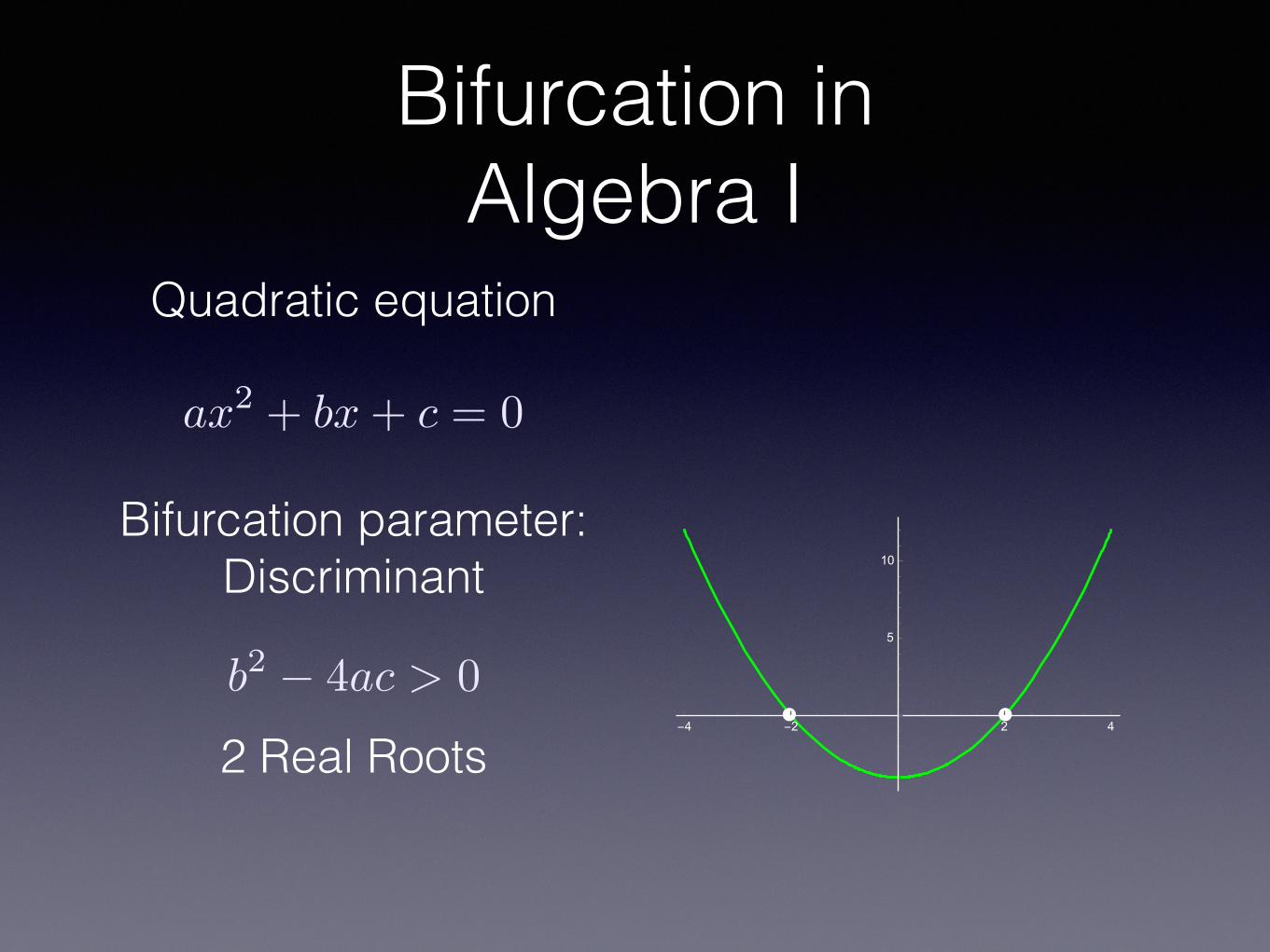
Bifurcation in Algebra I
Bifurcation parameter: Discriminant
b2 � 4ac > 0
2 Real Roots
Quadratic equation
ax
2 + bx+ c = 0
-4 -2 2 4
5
10

Bifurcation in Algebra I
Bifurcation parameter: Discriminant
b2 � 4ac > 0
2 Real Roots
Quadratic equation
ax
2 + bx+ c = 0
No qualitative change for small change
in equation
-4 -2 2 4
-5
5
10
15
Bifurcation in Algebra I
Bifurcation parameter: Discriminant
0 Real Roots
Quadratic equation
ax
2 + bx+ c = 0
Big enough change in system leads to
qualitatively different solutions
b2 � 4ac < 0
-4 -2 2 4
-5
5
10
15
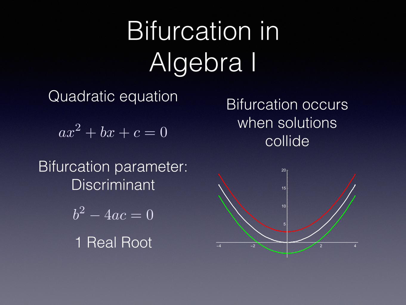
Bifurcation in Algebra I
Bifurcation parameter: Discriminant
1 Real Root
Quadratic equation
ax
2 + bx+ c = 0
Bifurcation occurs when solutions
collide
b2 � 4ac = 0
-4 -2 2 4
5
10
15
20
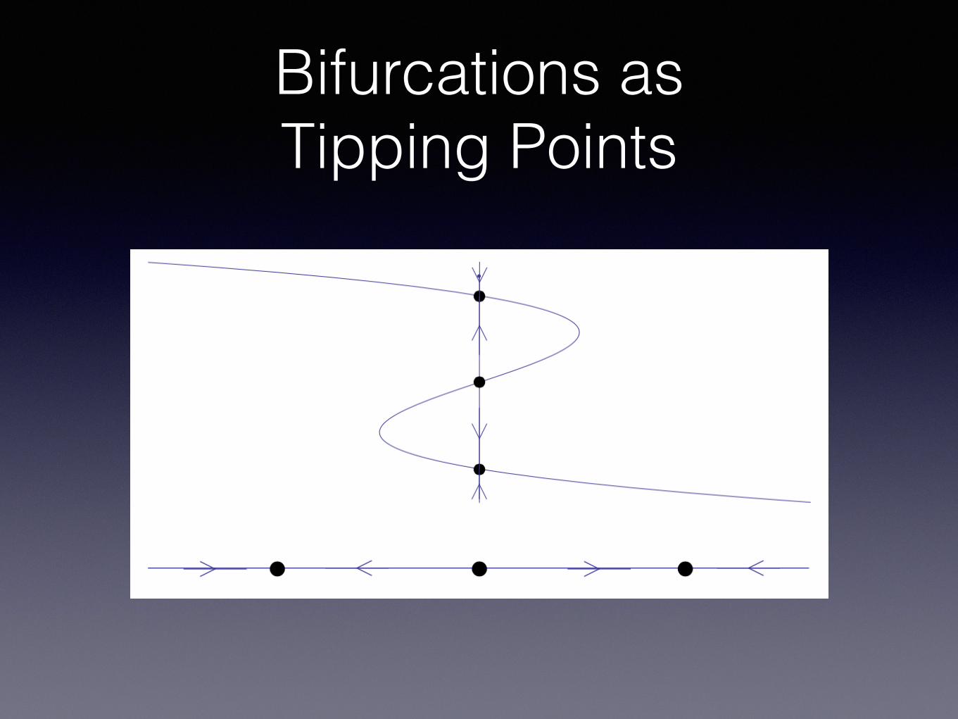
Bifurcations as Tipping Points

Bifurcations as Tipping Points

Bifurcations as Tipping Points

Bifurcations as Tipping Points
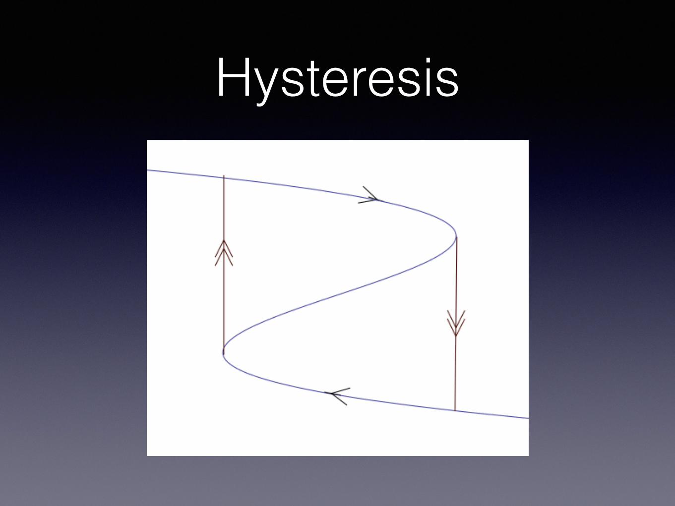
Hysteresis
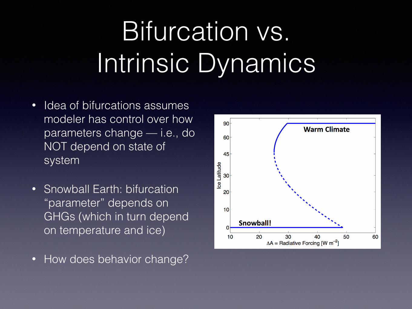
Bifurcation vs. Intrinsic Dynamics
• Idea of bifurcations assumes modeler has control over how parameters change — i.e., do NOT depend on state of system
• Snowball Earth: bifurcation “parameter” depends on GHGs (which in turn depend on temperature and ice)
• How does behavior change?
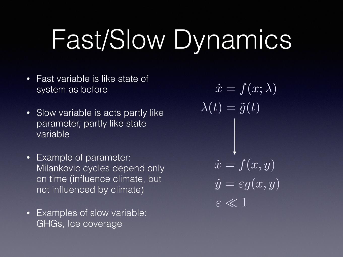
Fast/Slow Dynamics• Fast variable is like state of
system as before
• Slow variable is acts partly like parameter, partly like state variable
• Example of parameter: Milankovic cycles depend only on time (influence climate, but not influenced by climate)
• Examples of slow variable: GHGs, Ice coverage
x = f(x, y)
y = "g(x, y)
" ⌧ 1
x = f(x;�)
�(t) = g(t)
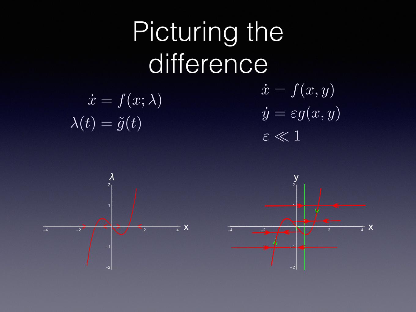
Picturing the difference
x = f(x;�)
�(t) = g(t)
-4 -2 2 4 x
-2
-1
1
2λ
x = f(x, y)
y = "g(x, y)
" ⌧ 1
-4 -2 2 4 x
-2
-1
1
2y
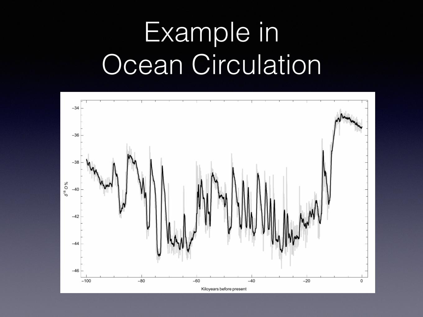
Example in Ocean Circulation

Stommel’s Circulation Model
Circulation variable:

Stommel’s Circulation Model
y = µ� y �A|1� y|y
y ⇠ Se � Sp
x ⇠ Te � Tp ! 1Model Reduces:
Get one state variable:
Bifurcation parameter:
µ ⇠ �SA
�TA

µ ! slow variable
y = µ� y �A|1� y|yµ = �0(�� y)
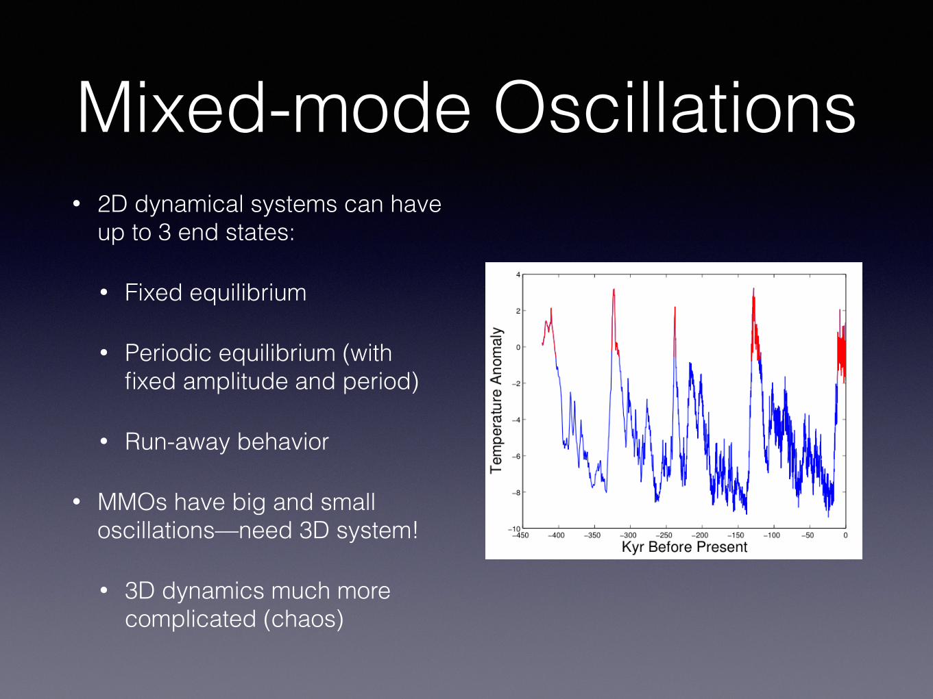
Mixed-mode Oscillations• 2D dynamical systems can have
up to 3 end states:
• Fixed equilibrium
• Periodic equilibrium (with fixed amplitude and period)
• Run-away behavior
• MMOs have big and small oscillations—need 3D system!
• 3D dynamics much more complicated (chaos)

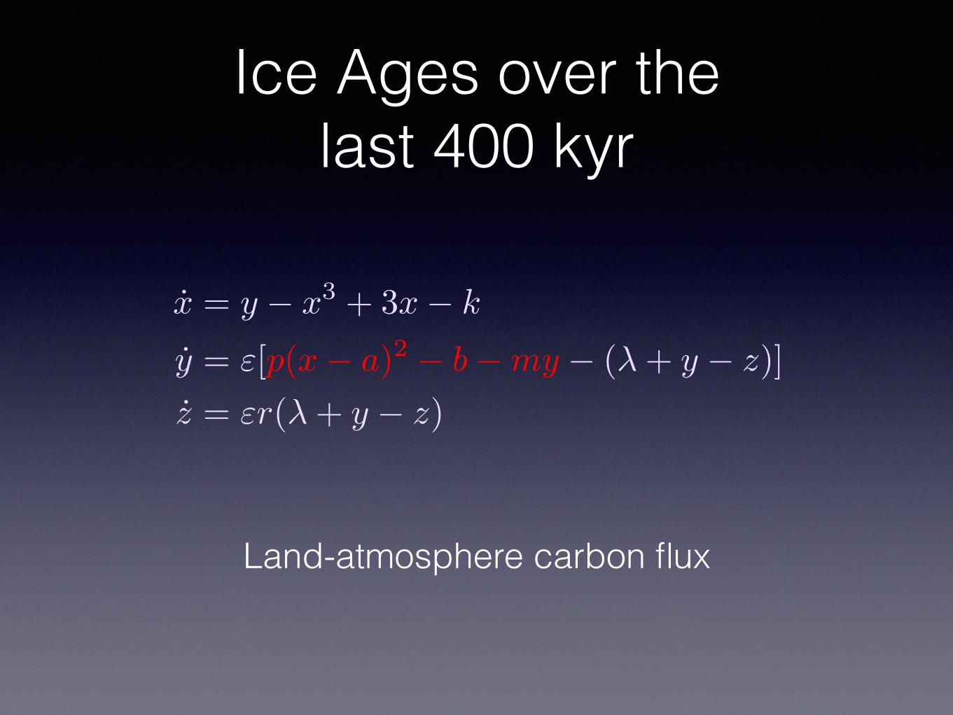
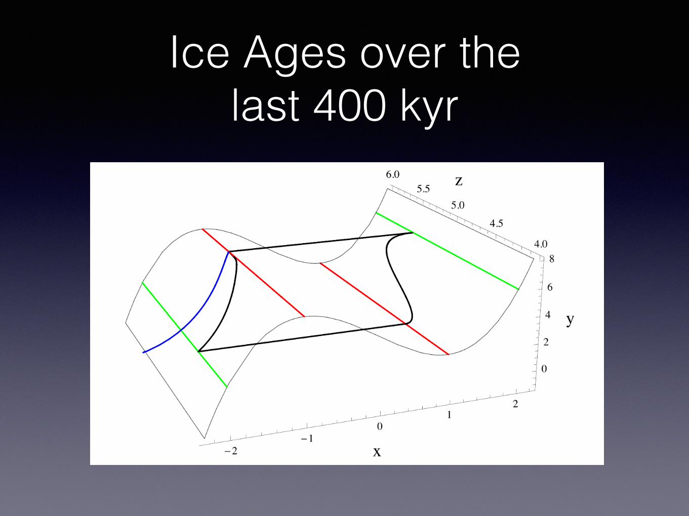
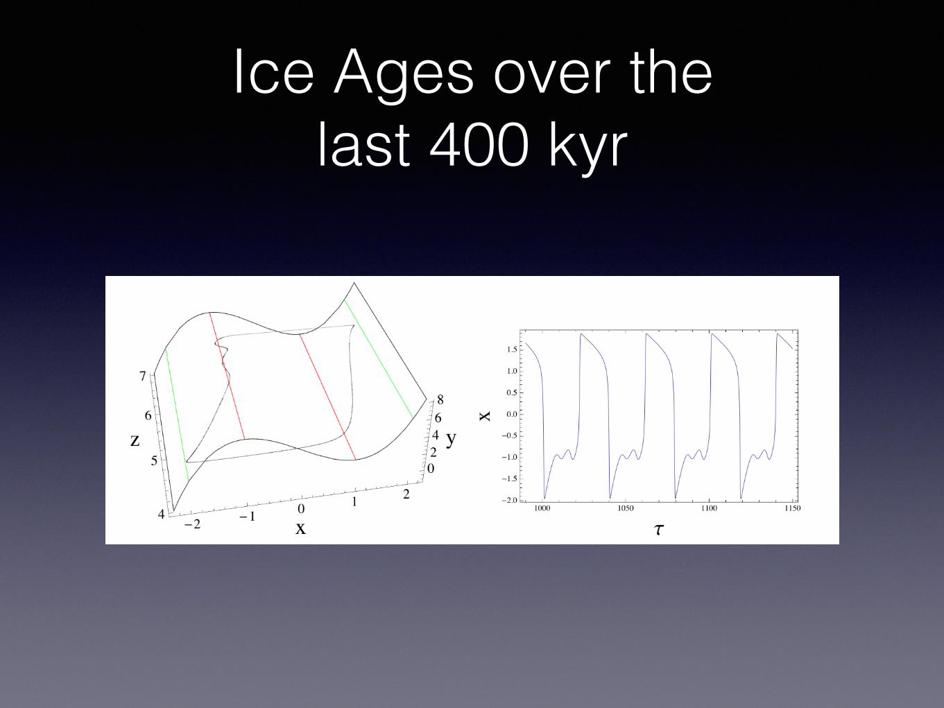
Ice Ages over the last 400 kyr
x = y � x
3 + 3x� k
y = "[p(x� a)2 � b�my � (�+ y � z)]
z = "r(�+ y � z)

Ice Ages over the last 400 kyr
x = y � x
3 + 3x� k
y = "[p(x� a)2 � b�my � (�+ y � z)]
z = "r(�+ y � z)
ice volume
atmospheric carbon
oceanic carbonx ⇠
y ⇠
z ⇠

Ice Ages over the last 400 kyr
x = y � x
3 + 3x� k
y = "[p(x� a)2 � b�my � (�+ y � z)]
z = "r(�+ y � z)
Fast Slow

Ice Ages over the last 400 kyr
x = y � x
3 + 3x� k
y = "[p(x� a)2 � b�my � (�+ y � z)]
z = "r(�+ y � z)
Change in ice volume depends on temperature, but temperature depends on the amount of ice
and how much GHGs are in the atmosphere
Ice Ages over the last 400 kyr
x = y � x
3 + 3x� k
y = "[p(x� a)2 � b�my � (�+ y � z)]
z = "r(�+ y � z)
Land-atmosphere carbon flux
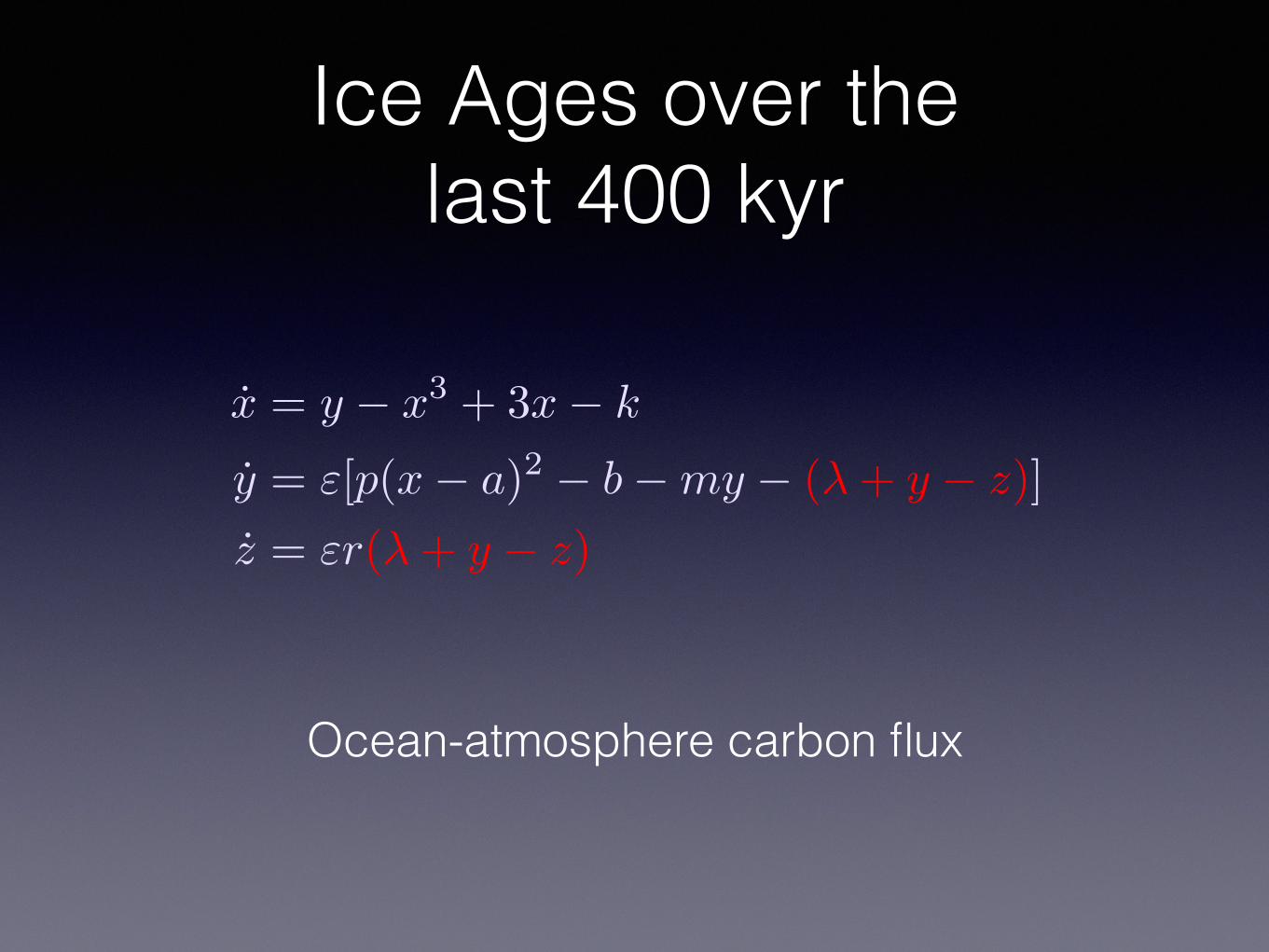
Ice Ages over the last 400 kyr
Ocean-atmosphere carbon flux
x = y � x
3 + 3x� k
y = "[p(x� a)2 � b�my � (�+ y � z)]
z = "r(�+ y � z)
Ice Ages over the last 400 kyr
Ice Ages over the last 400 kyr

Ice Ages over the last 400 kyr
Ice Ages over the last 400 kyr

Ice Ages over the last 400 kyr
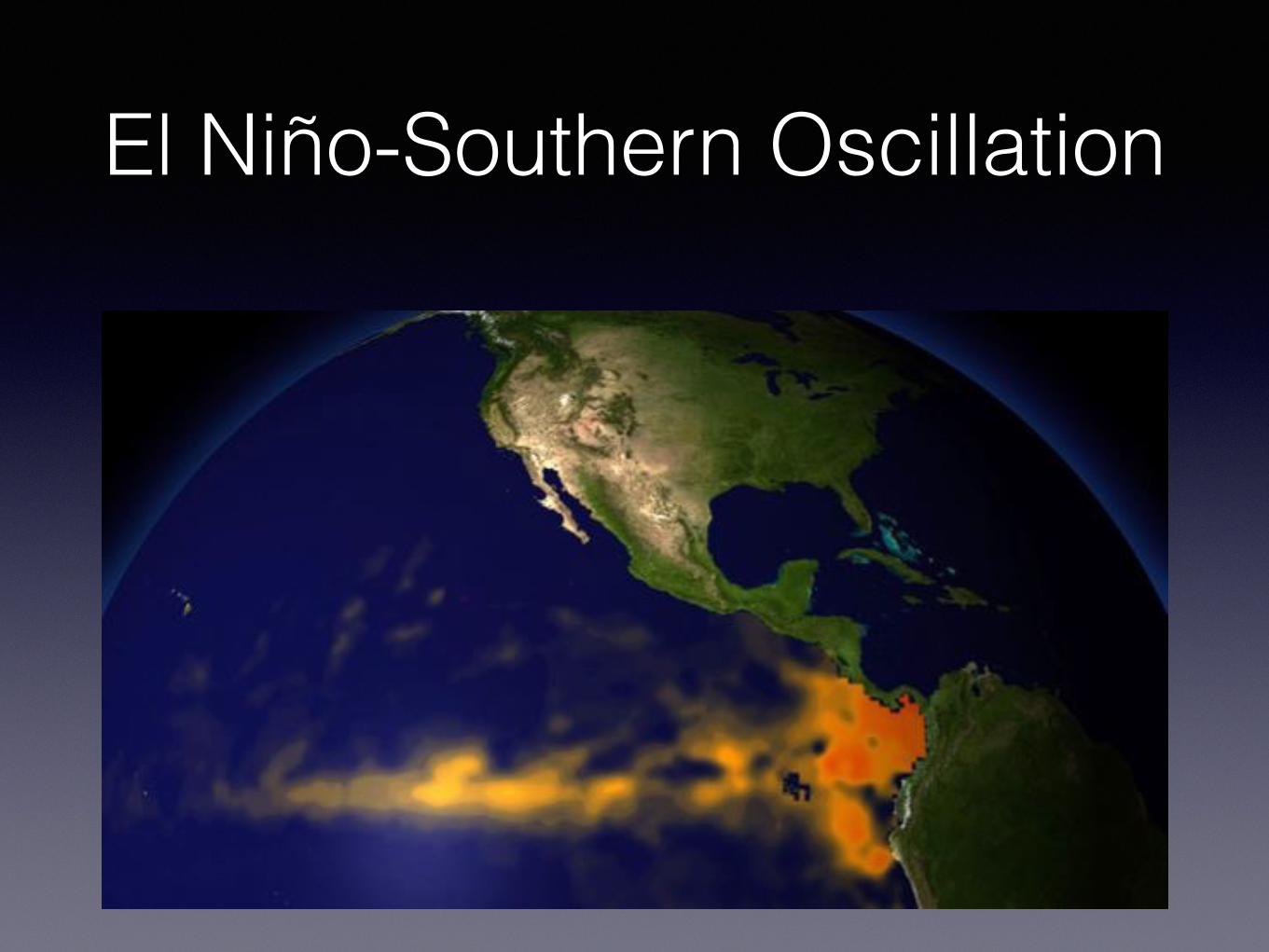
El Niño-Southern Oscillation

How does ENSO work?

The Data

Predicting ENSOAugust predictions
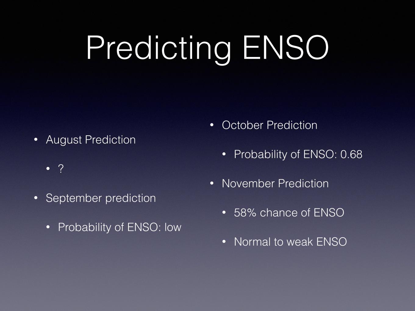
Predicting ENSO
• August Prediction
• ?
• September prediction
• Probability of ENSO: low
• October Prediction
• Probability of ENSO: 0.68
• November Prediction
• 58% chance of ENSO
• Normal to weak ENSO
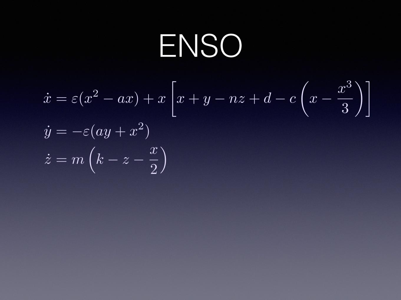
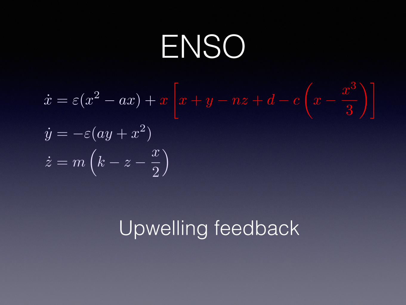
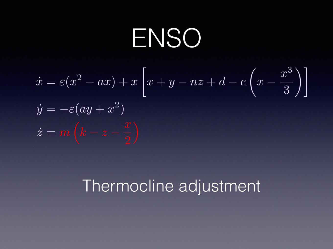
ENSOx = "(x2 � ax) + x
x+ y � nz + d� c
✓x� x
3
3
◆�
y = �"(ay + x
2)
z = m
⇣k � z � x
2
⌘

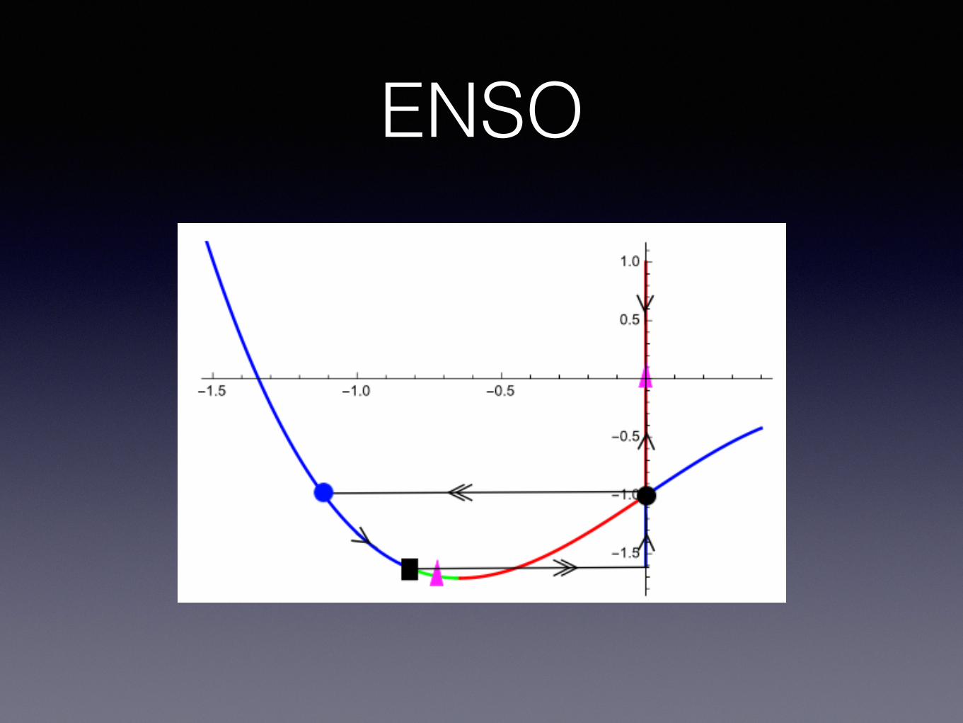
ENSO
x
z
temperature gradient
temp of W Pacific
thermocline dept in W Pacific
x = "(x2 � ax) + x
x+ y � nz + d� c
✓x� x
3
3
◆�
y = �"(ay + x
2)
z = m
⇣k � z � x
2
⌘
y
ENSOx = "(x2 � ax) + x
x+ y � nz + d� c
✓x� x
3
3
◆�
y = �"(ay + x
2)
z = m
⇣k � z � x
2
⌘
Upwelling feedback
ENSO
Thermocline adjustment
x = "(x2 � ax) + x
x+ y � nz + d� c
✓x� x
3
3
◆�
y = �"(ay + x
2)
z = m
⇣k � z � x
2
⌘

ENSO
Advection
x = "(x2 � ax) + x
x+ y � nz + d� c
✓x� x
3
3
◆�
y = �"(ay + x
2)
z = m
⇣k � z � x
2
⌘
ENSO
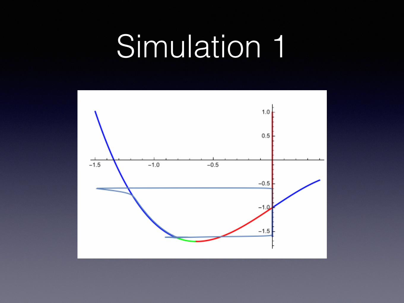
Simulation 1
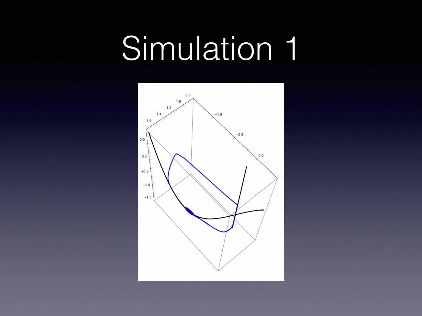
Simulation 1

Simulation 2

Simulation 2
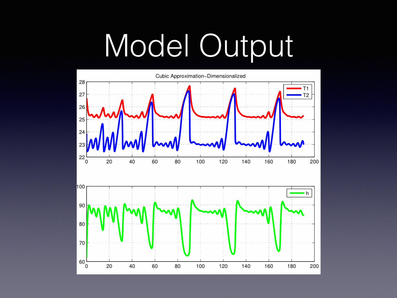
Model Output
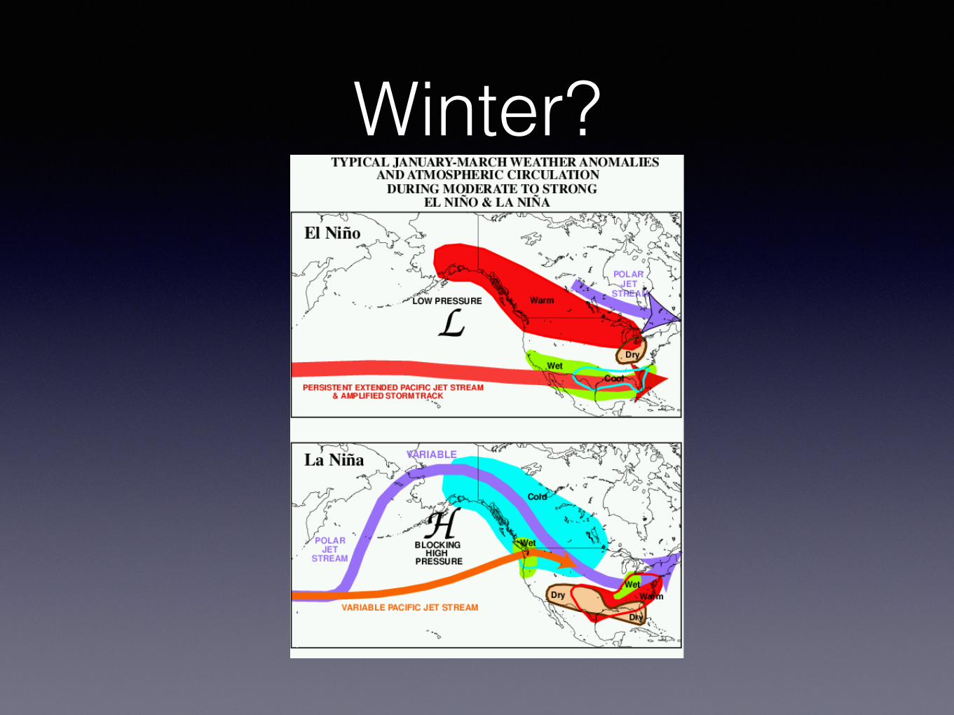
Winter?