matlab course - part ii: modelling, simulation and … · and control applications. this is a...
TRANSCRIPT
University of South-Eastern Norway
MATLAB Part II: Modelling, Simulation & Control
Hans-Petter Halvorsen, 2018.08.27
http://www.halvorsen.blog

ii
Preface
Copyright You cannot distribute or copy this document without permission from the author.
You cannot copy or link to this document directly from other sources, web pages, etc. You
should always link to the proper web page where this document is located, typically
http://www.halvorsen.blog
In this MATLAB Course, you will learn basic MATLAB and how to use MATLAB in Control and
Simulation applications. An introduction to Simulink and other Tools will also be given.
MATLAB is a tool for technical computing, computation and visualization in an integrated
environment. MATLAB is an abbreviation for MATrix LABoratory, so it is well suited for
matrix manipulation and problem solving related to Linear Algebra, Modelling, Simulation
and Control applications.
This is a self-paced course based on this document and some short videos on the way. This
document contains lots of examples and self-paced tasks that the users will go through and
solve on their own. The user may go through the tasks in this document in their own pace
and the instructor will be available for guidance throughout the course.
The MATLAB Course consists of 3 parts:
• MATLAB Course – Part I: Introduction to MATLAB
• MATLAB Course – Part II: Modelling, Simulation and Control
• MATLAB Course – Part III: Simulink and Advanced Topics
In Part II of the course (Part II: Modelling, Control and Simulation) you will learn how to use
MATLAB in Modelling, Control and Simulation.
You must go through MATLAB Course – Part I: Introduction to MATLAB before you start.
The course consists of lots of Tasks you should solve while reading this course manual and
watching the videos referred to in the text.
Make sure to bring your headphones for the videos in this course. The
course consists of several short videos that will give you an introduction to the different
topics in the course.
iii
Prerequisites
You should be familiar with undergraduate-level mathematics and have experience with
basic computer operations.
What is MATLAB? MATLAB is a tool for technical computing, computation and visualization
in an integrated environment. MATLAB is an abbreviation for MATrix LABoratory, so it is well
suited for matrix manipulation and problem solving related to Linear Algebra.
MATLAB is developed by The MathWorks. MATLAB is a short-term for MATrix LABoratory.
MATLAB is in use world-wide by researchers and universities. For more information, see
www.mathworks.com
For more information about MATLAB, etc., please visit http://www.halvorsen.blog
Online MATLAB Resources:
MATLAB:
http://www.halvorsen.blog/documents/programming/matlab/
MATLAB Basics:
http://www.halvorsen.blog/documents/programming/matlab/matlab_basics.php
Modelling, Simulation and Control with MATLAB:
http://www.halvorsen.blog/documents/programming/matlab/matlab_mic.php
MATLAB Videos:
http://www.halvorsen.blog/documents/video/matlab_basics_videos.php
MATLAB for Students:
http://www.halvorsen.blog/documents/teaching/courses/matlab.php
On these web pages you find video solutions, complete step by step solutions, downloadable
MATLAB code, additional resources, etc.
iv
Table of Contents
Preface ........................................................................................................................................ ii
Table of Contents ...................................................................................................................... iv
1 Introduction ........................................................................................................................ 1
2 Differential Equations and ODE Solvers ............................................................................. 2
2.1 ODE Solvers in MATLAB .............................................................................................. 4
Task 1: Bacteria Population ........................................................................................ 6
Task 2: Passing Parameters to the model .................................................................. 7
Task 3: ODE Solvers .................................................................................................... 8
Task 4: 2. order differential equation ......................................................................... 8
3 Discrete Systems .............................................................................................................. 10
3.1 Discretization ............................................................................................................ 10
Task 5: Discrete Simulation ...................................................................................... 13
Task 6: Discrete Simulation – Bacteria Population ................................................... 13
Task 7: Simulation with 2 variables .......................................................................... 14
4 Numerical Techniques ...................................................................................................... 19
4.1 Interpolation ............................................................................................................. 19
Task 8: Interpolation ................................................................................................. 21
4.2 Curve Fitting ............................................................................................................. 22
4.2.1 Linear Regression ............................................................................................. 22
Task 9: Linear Regression ......................................................................................... 24
4.2.2 Polynomial Regression ..................................................................................... 25
Task 10: Polynomial Regression ............................................................................. 27

v Table of Contents
MATLAB Course - Part II: Modelling, Simulation and Control
Task 11: Model fitting ............................................................................................. 27
4.3 Numerical Differentiation ........................................................................................ 27
Task 12: Numerical Differentiation ........................................................................ 32
4.3.1 Differentiation on Polynomials ........................................................................ 32
Task 13: Differentiation on Polynomials ................................................................ 33
Task 14: Differentiation on Polynomials ................................................................ 34
4.4 Numerical Integration .............................................................................................. 34
Task 15: Numerical Integration .............................................................................. 37
4.4.1 Integration on Polynomials .............................................................................. 38
Task 16: Integration on Polynomials ...................................................................... 38
5 Optimization ..................................................................................................................... 39
Task 17: Optimization ............................................................................................. 42
Task 18: Optimization - Rosenbrock's Banana Function ........................................ 42
6 Control System Toolbox ................................................................................................... 44
7 Transfer Functions ............................................................................................................ 46
7.1 Introduction .............................................................................................................. 46
Task 19: Transfer function ...................................................................................... 48
7.2 Second order Transfer Function ............................................................................... 48
Task 20: 2.order Transfer function ......................................................................... 49
Task 21: Time Response ......................................................................................... 50
7.3 Analysis of Standard Functions ................................................................................ 50
Task 22: Integrator ................................................................................................. 50
Task 23: 1. order system ......................................................................................... 51
Task 24: 2. order system ......................................................................................... 51
Task 25: 2. order system – Special Case ................................................................. 52
8 State-space Models .......................................................................................................... 54

vi Table of Contents
MATLAB Course - Part II: Modelling, Simulation and Control
8.1 Introduction .............................................................................................................. 54
8.2 Tasks ......................................................................................................................... 56
Task 26: State-space model .................................................................................... 56
Task 27: Mass-spring-damper system .................................................................... 56
Task 28: Block Diagram ........................................................................................... 57
8.3 Discrete State-space Models .................................................................................... 58
Task 29: Discretization ............................................................................................ 58
9 Frequency Response ........................................................................................................ 60
9.1 Introduction .............................................................................................................. 60
9.2 Tasks ......................................................................................................................... 63
Task 30: 1. order system ......................................................................................... 63
Task 31: Bode Diagram ........................................................................................... 63
9.3 Frequency response Analysis ................................................................................... 64
9.3.1 Loop Transfer Function .................................................................................... 64
9.3.2 Tracking Transfer Function ............................................................................... 65
9.3.3 Sensitivity Transfer Function ............................................................................ 65
Task 32: Frequency Response Analysis .................................................................. 66
9.4 Stability Analysis of Feedback Systems .................................................................... 67
Task 33: Stability Analysis ....................................................................................... 69
10 Additional Tasks ........................................................................................................... 70
Task 34: ODE Solvers .............................................................................................. 70
Task 35: Mass-spring-damper system .................................................................... 70
Task 36: Numerical Integration .............................................................................. 71
Task 37: State-space model .................................................................................... 72
Task 38: lsim ........................................................................................................... 72
Appendix A – MATLAB Functions ............................................................................................. 74

vii Table of Contents
MATLAB Course - Part II: Modelling, Simulation and Control
Numerical Techniques .......................................................................................................... 74
Solving Ordinary Differential Equations ........................................................................... 74
Interpolation ..................................................................................................................... 74
Curve Fitting ..................................................................................................................... 74
Numerical Differentiation ................................................................................................ 75
Numerical Integration ...................................................................................................... 75
Optimization ......................................................................................................................... 75
Control and Simulation......................................................................................................... 76
1
1 Introduction
Additional Resources, Videos, etc. are available from:
http://www.halvorsen.blog/documents/programming/matlab
Part 2: “Modelling, Simulation and Control” consists of the following topics:
• Differential Equations and ODE Solvers
• Discrete Systems
• Numerical Techniques
o Interpolation
o Curve Fitting
o Numerical Differentiation
o Numerical Integration
• Optimization
• Control System Toolbox
• Transfer functions
• State-space models
• Frequency Response

2
2 Differential Equations and
ODE Solvers
MATLAB have lots of built-in functionality for solving differential equations. MATLAB
includes functions that solve ordinary differential equations (ODE) of the form:
𝑑𝑦
𝑑𝑡= 𝑓(𝑡, 𝑦), 𝑦(𝑡0) = 𝑦0
MATLAB can solve these equations numerically.
Higher order differential equations must be reformulated into a system of first order
differential equations.
Note! Different notation is used:
𝑑𝑦
𝑑𝑡= 𝑦′ = �̇�
This document will use these different notations interchangeably.
Not all differential equations can be solved by the same technique, so MATLAB offers lots of
different ODE solvers for solving differential equations, such as ode45, ode23, ode113, etc.
Example:
Given the following differential equation:
�̇� = 𝑎𝑥
where 𝑎 = −1
𝑇 ,where 𝑇 is the time constant
Note! �̇� =𝑑𝑥
𝑑𝑡
The solution for the differential equation is found to be:
𝑥(𝑡) = 𝑒𝑎𝑡𝑥0
We shall plot the solution for this differential equation using MATLAB.
Set 𝑇 = 5 and the initial condition 𝑥(0) = 1.

3 Differential Equations and ODE Solvers
MATLAB Course - Part II: Modelling, Simulation and Control
We will create a script in MATLAB (.m file) where we plot the solution 𝑥(𝑡) in the time
interval 0 ≤ 𝑡 ≤ 25
The Code is as follows:
T = 5;
a = -1/T;
x0 = 1;
t = [0:1:25]
x = exp(a*t)*x0;
plot(t,x);
grid
This gives the following Results:
[End of Example]
This works fine, but the problem is that we first have to find the solution to the differential
equation – instead we can use one of the built-in solvers for Ordinary Differential Equations
(ODE) in MATLAB.
There are different functions, such as ode23 and ode45.
Example:
We use the ode23 solver in MATLAB for solving the differential equation (“runmydiff.m”):
tspan = [0 25];
x0 = 1;

4 Differential Equations and ODE Solvers
MATLAB Course - Part II: Modelling, Simulation and Control
[t,x] = ode23(@mydiff,tspan,x0);
plot(t,x)
Where @mydiff is defined as a function like this (“mydiff.m”):
function dx = mydiff(t,x)
a = -1/5;
dx = a*x;
This gives the same results as shown in the plot above and MATLAB have solved the
differential equation for us (numerically).
Note! You have to implement it in 2 different m. files, one m. file where you define the
differential equation you are solving, and another .m file where you solve the equation using
the ode23 solver.
[End of Example]
2.1 ODE Solvers in MATLAB
All of the ODE solver functions share a syntax that makes it easy to try any of the different
numerical methods, if it is not apparent which is the most appropriate. To apply a different
method to the same problem, simply change the ODE solver function name. The simplest
syntax, common to all the solver functions, is:
[t,y] = solver(odefun,tspan,y0,options,…)
where “solver” is one of the ODE solver functions (ode23, ode45, etc.).
Note! If you don’t specify the resulting array [t, y], the function create a plot of the result.
‘odefun’ is the function handler, which is a “nickname” for your function that contains the
differential equations.
Example:
Given the differential equations:
𝑑𝑦
𝑑𝑡= 𝑥
𝑑𝑥
𝑑𝑡= −𝑦
In MATLAB you define a function for these differential equations:
5 Differential Equations and ODE Solvers
MATLAB Course - Part II: Modelling, Simulation and Control
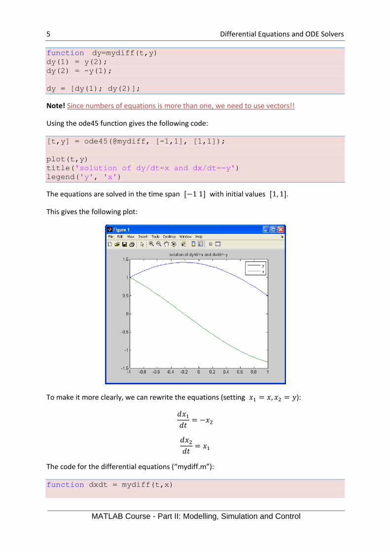
function dy=mydiff(t,y)
dy(1) = y(2);
dy(2) = -y(1);
dy = [dy(1); dy(2)];
Note! Since numbers of equations is more than one, we need to use vectors!!
Using the ode45 function gives the following code:
[t,y] = ode45(@mydiff, [-1,1], [1,1]);
plot(t,y)
title('solution of dy/dt=x and dx/dt=-y')
legend('y', 'x')
The equations are solved in the time span [−1 1] with initial values [1, 1].
This gives the following plot:
To make it more clearly, we can rewrite the equations (setting 𝑥1 = 𝑥, 𝑥2 = 𝑦):
𝑑𝑥1𝑑𝑡
= −𝑥2
𝑑𝑥2𝑑𝑡
= 𝑥1
The code for the differential equations (“mydiff.m”):
function dxdt = mydiff(t,x)

6 Differential Equations and ODE Solvers
MATLAB Course - Part II: Modelling, Simulation and Control
dxdt(1) = -x(2);
dxdt(2) = x(1);
dxdt = dxdt';
Note! The function mydiff must return a column vector, that’s why we need to transpose it.
Then we use the ode solver to solve the differential equations (“run_mydiff.m”):
tspan = [-1,1];
x0 = [1,1];
[t,x] = ode45(@mydiff, tspan, x0);
plot (t,x)
legend('x1', 'x2')
The solution will be the same.
[End of Example]
Task 1: Bacteria Population
In this task we will simulate a simple model of a bacteria population in a jar.
The model is as follows:
birth rate=bx
death rate = px2
Then the total rate of change of bacteria population is:
�̇� = 𝑏𝑥 − 𝑝𝑥2
Set b=1/hour and p=0.5 bacteria-hour
Note! �̇� =𝑑𝑥
𝑑𝑡
→ Simulate (i.e., create a plot) the number of bacteria in the jar after 1 hour, assuming that
initially there are 100 bacteria present.
How many bacteria are present after 1 hour?
[End of Task]

7 Differential Equations and ODE Solvers
MATLAB Course - Part II: Modelling, Simulation and Control
Task 2: Passing Parameters to the model
Given the following system:
�̇� = 𝑎𝑥 + 𝑏
where 𝑎 = −1
𝑇 ,where 𝑇 is the time constant
In this case we want to pass 𝑎 and 𝑏 as parameters, to make it easy to be able to change
values for these parameters.
We set initial condition 𝑥(0) = 1 and 𝑇 = 5.
The function for the differential equation is:
function dx = mysimplediff(t,x,param)
% My Simple Differential Equation
a = param(1);
b = param(2);
dx = a*x+b;
Then we solve and plot the equation using this code:
tspan = [0 25];
x0 = 1;
a = -1/5;
b = 1;
param = [a b];
[t,y] = ode45(@mysimplediff, tspan, x0,[], param);
plot(t,y)
By doing this, it is very easy to changes values for the parameters 𝑎 and 𝑏 without
changing the code for the differential equation.
Note! We need to use the 5. argument in the ODE solver function for this. The 4. argument is
for special options and is normally set to “[]”, i.e., no options.
The result from the simulation is:

8 Differential Equations and ODE Solvers
MATLAB Course - Part II: Modelling, Simulation and Control
→ Write the code above
Read more about the different solvers that exists in the Help system in MATLAB
[End of Task]
Task 3: ODE Solvers
Use the ode23 function to solve and plot the results of the following differential equation in
the interval [𝑡0, 𝑡𝑓]:
𝒘′ + (𝟏. 𝟐 + 𝒔𝒊𝒏𝟏𝟎𝒕)𝒘 = 𝟎, 𝑡0 = 0, 𝑡𝑓 = 5,𝑤(𝑡0) = 1
Note! 𝑤′ =𝑑𝑤
𝑑𝑡
[End of Task]
Task 4: 2. order differential equation
Use the ode23/ode45 function to solve and plot the results of the following differential
equation in the interval [𝑡0, 𝑡𝑓]:
(𝟏 + 𝒕𝟐)�̈� + 𝟐𝒕�̇� + 𝟑𝒘 = 𝟐, 𝑡0 = 0, 𝑡𝑓 = 5,𝑤(𝑡0) = 0, �̇�(𝑡0) = 1
Note! �̈� =𝑑2𝑤
𝑑𝑡2

9 Differential Equations and ODE Solvers
MATLAB Course - Part II: Modelling, Simulation and Control
Note! Higher order differential equations must be reformulated into a system of first order
differential equations.
Tip 1: Reformulate the differential equation so �̈� is alone on the left side.
Tip 2: Set:
𝑤 = 𝑥1
�̇� = 𝑥2
[End of Task]

10
3 Discrete Systems
MATLAB has built-in powerful features for simulation of continuous differential equations
and dynamic systems.
Sometimes we want to or need to discretize a continuous system and then simulate it in
MATLAB.
When dealing with computer simulation, we need to create a discrete version of our system.
This means we need to make a discrete version of our continuous differential equations.
Actually, the built-in ODE solvers in MATLAB use different discretization methods.
Interpolation, Curve Fitting, etc. is also based on a set of discrete values (data points or
measurements). The same with Numerical Differentiation and Numerical Integration, etc.
Below we see a continuous signal vs the discrete signal for a given system with discrete time
interval 𝑇𝑠 = 0.1𝑠.
3.1 Discretization
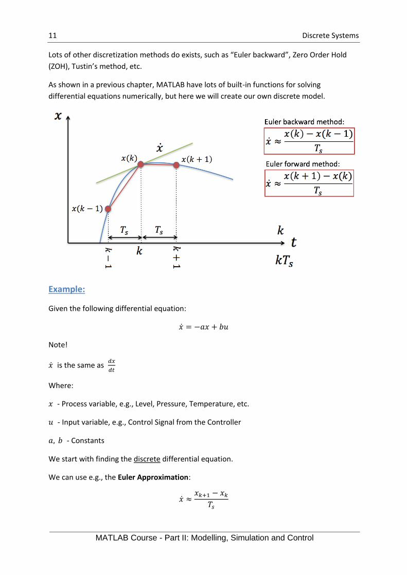
In order to discretize a continuous model there are lots of different methods to use. One of
the simplest is Euler Forward method:
�̇� ≈𝑥𝑘+1 − 𝑥𝑘
𝑇𝑠
where 𝑇𝑠 is the sampling time.
11 Discrete Systems
MATLAB Course - Part II: Modelling, Simulation and Control
Lots of other discretization methods do exists, such as “Euler backward”, Zero Order Hold
(ZOH), Tustin’s method, etc.
As shown in a previous chapter, MATLAB have lots of built-in functions for solving
differential equations numerically, but here we will create our own discrete model.
Example:
Given the following differential equation:
�̇� = −𝑎𝑥 + 𝑏𝑢
Note!
�̇� is the same as 𝑑𝑥
𝑑𝑡
Where:
𝑥 - Process variable, e.g., Level, Pressure, Temperature, etc.
𝑢 - Input variable, e.g., Control Signal from the Controller
𝑎, 𝑏 - Constants
We start with finding the discrete differential equation.
We can use e.g., the Euler Approximation:
�̇� ≈𝑥𝑘+1 − 𝑥𝑘
𝑇𝑠

12 Discrete Systems
MATLAB Course - Part II: Modelling, Simulation and Control
𝑇𝑠 - Sampling Interval
Then we get:
𝑥𝑘+1 − 𝑥𝑘𝑇𝑠
= −𝑎𝑥𝑘 + 𝑏𝑢𝑘
This gives the following discrete differential equation:
𝑥𝑘+1 = (1 − 𝑇𝑠𝑎)𝑥𝑘 + 𝑇𝑠𝑏𝑢𝑘
Now we are ready to simulate the system
We set 𝑎 = 0.25, 𝑏 = 2 and 𝑢 = 1 (You can explore with other values on your own)
The Code can be written as follows:
% Simulation of discrete model
clear, clc
% Model Parameters
a = 0.25;b = 2;
% Simulation Parameters
Ts = 0.1; %s
Tstop = 30; %s
uk = 1; % Step Response
x(1) = 0;
% Simulation
for k=1:(Tstop/Ts)
x(k+1) = (1-a*Ts).*x(k) + Ts*b*uk;
end
% Plot the Simulation Results
k=0:Ts:Tstop;
plot(k,x)
grid on
This gives the following Results:
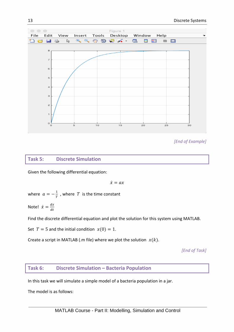
13 Discrete Systems
MATLAB Course - Part II: Modelling, Simulation and Control
[End of Example]
Task 5: Discrete Simulation
Given the following differential equation:
�̇� = 𝑎𝑥
where 𝑎 = −1
𝑇 , where 𝑇 is the time constant
Note! �̇� =𝑑𝑥
𝑑𝑡
Find the discrete differential equation and plot the solution for this system using MATLAB.
Set 𝑇 = 5 and the initial condition 𝑥(0) = 1.
Create a script in MATLAB (.m file) where we plot the solution 𝑥(𝑘).
[End of Task]
Task 6: Discrete Simulation – Bacteria Population
In this task we will simulate a simple model of a bacteria population in a jar.
The model is as follows:

14 Discrete Systems
MATLAB Course - Part II: Modelling, Simulation and Control
birth rate = bx
death rate = px2
Then the total rate of change of bacteria population is:
�̇� = 𝑏𝑥 − 𝑝𝑥2
Set b=1/hour and p=0.5 bacteria-hour
We will simulate the number of bacteria in the jar after 1 hour, assuming that initially there
are 100 bacteria present.
→ Find the discrete model using the Euler Forward method by hand and implement and
simulate the system in MATLAB using a For Loop.
[End of Task]
Task 7: Simulation with 2 variables
Given the following system
𝑑𝑥1𝑑𝑡
= −𝑥2
𝑑𝑥2𝑑𝑡
= 𝑥1
Find the discrete system and simulate the discrete system in MATLAB.
Solve the equations, e.g., in the time span [−1 1] with initial values [1, 1].
[End of Task]
3.2 Code Optimization
Example:
When doing more advanced simulations, it is important that you spend time optimization
your code. In the examples and tasks above the equations are quite simple, but when the
equations become more complicated, or your simulation time increases, code optimization
becomes more important.

15 Discrete Systems
MATLAB Course - Part II: Modelling, Simulation and Control
In the code example below the following simple differential equation will be used:
�̇� = 𝑎𝑥 + 𝑏𝑢
But we will increase the simulation time dramatically compared to the previous examples.
MATLAB Code 1;
clear, clc
tic
a=-10; b=0.5;
x=0; u=1;
dt=0.01;
N=1000000000;
X(1)=x;
for i=1:N
X(i+1)=X(i)+dt*(a*X(i)+b*u);
end
toc
MATLAB Code 2:
clear, clc
tic
a=-10; b=0.5;
x=0; u=1;
dt=0.01;
N=1000000000;
X=zeros(N,1);
for i=1:N
X(i+1)=X(i)+dt*(a*X(i)+b*u);
end
toc
MATLAB Code 3:
clear, clc
tic
a=-10; b=0.5;
x=0; u=1;
dt=0.01;
N=1000000000;

16 Discrete Systems
MATLAB Course - Part II: Modelling, Simulation and Control
X=zeros(N,1);
for i=1:N
X(i)=x;
x=x+dt*(a*x+b*u);
end
toc
Try the different code examples and note the execution time. Try with different values of N,
etc.
[End of Example]
Example:
In the code example below the following simple differential equation will be used:
�̇� = −𝑎𝑥 + 𝑏𝑢
MATLAB Code 1;
% Simulation of discrete model
clear, clc
% Model Parameters
a = 0.25;b = 2;
% Simulation Parameters
Ts = 0.01;
Tstop = 10000000;
x(1) = 0;
N = Tstop/Ts;
u = linspace(0,1,N);
% Simulation
tic
for k=1:N
x(k+1) = (1-a*Ts).*x(k) + Ts*b*u(k);
end
toc
% Plot the Simulation Results
t=0:Ts:Tstop;
plot(t,x)
grid on
MATLAB Code 2:
% Simulation of discrete model
clear, clc

17 Discrete Systems
MATLAB Course - Part II: Modelling, Simulation and Control
% Model Parameters
a = 0.25;b = 2;
% Simulation Parameters
Ts = 0.01;
Tstop = 10000000;
uk = 1;
N = Tstop/Ts;
u = linspace(0,1,N);
%Preallocation
x = zeros(N,1);
% Simulation
tic
for k=1:N
x(k+1) = (1-a*Ts).*x(k) + Ts*b*u(k);
end
toc
% Plot the Simulation Results
t=0:Ts:Tstop;
plot(t,x)
grid on
MATLAB Code 3:
% Simulation of discrete model
clear, clc
% Model Parameters
a = 0.25;b = 2;
% Simulation Parameters
Ts = 0.01;
Tstop = 10000000;
uk = 1;
x = 0;
X(1)=x;
N = Tstop/Ts;
u = rand(N,1);
u = linespace(0,1,N);
% Simulation
X = zeros(N,1);
tic
for k=1:N
x = (1-a*Ts)*x + Ts*b*u(k);
X(k+1)=x;
end
toc

18 Discrete Systems
MATLAB Course - Part II: Modelling, Simulation and Control
% Plot the Simulation Results
t=0:Ts:Tstop;
plot(t,X)
grid on
In general, it will be many ways to implement a given system in MATLAB, we can use built in
ODE solvers, we can use different discretization methods, and we can optimize our code in
other ways.
There is not a “best way” that can be used for all kind of systems. It will be your
responsibility to find the best solution for your system. That’s why it is important that you
know about different ways to do things, so you are able to find the best solution in a given
situation.
[End of Example]

19
4 Numerical Techniques
In the previous chapter we investigated how to solve differential equations numerically, in
this chapter we will take a closer look at some other numerical techniques offered by
MATLAB, such as interpolation, curve-fitting, numerical differentiations and integrations.
4.1 Interpolation
Interpolation is used to estimate data points between two known points. The most common
interpolation technique is Linear Interpolation.
In MATLAB we can use the interp1 function.
Example:
Given the following data:
x y
0 15
1 10
2 9
3 6
4 2
5 0
We will find the interpolated value for 𝑥 = 3.5.
The following MATLAB code will do this:
x=0:5;
y=[15, 10, 9, 6, 2, 0];
plot(x,y ,'-o')
% Find interpolated value for x=3.5
new_x=3.5;
new_y = interp1(x,y,new_x)
The answer is 4, from the plot below we see this is a good guess:

20 Numerical Techniques
MATLAB Course - Part II: Modelling, Simulation and Control
[End of Example]
The default is linear interpolation, but there are other types available, such as:
• linear
• nearest
• spline
• cubic
• etc.
Type “help interp1” in order to read more about the different options.
Example:
In this example we will use a spline interpolation on the same data as in the example above.
x=0:5;
y=[15, 10, 9,6, 2, 0];
new_x=0:0.2:5;
new_y=interp1(x,y,new_x, 'spline')
plot(x,y, new_x, new_y, '-o')
The result is as we plot both the original point and the interpolated points in the same
graph:

21 Numerical Techniques
MATLAB Course - Part II: Modelling, Simulation and Control
We see this result in 2 different lines.
[End of Example]
Task 8: Interpolation
Given the following data:
Temperature, T [ oC] Energy, u [KJ/kg]
100 2506.7
150 2582.8
200 2658.1
250 2733.7
300 2810.4
400 2967.9
500 3131.6
Plot u versus T. Find the interpolated data and plot it in the same graph. Test out different
interpolation types. Discuss the results. What kind of interpolation is best in this case?
What is the interpolated value for u=2680.78 KJ/kg?
[End of Task]
22 Numerical Techniques
MATLAB Course - Part II: Modelling, Simulation and Control
4.2 Curve Fitting
In the previous section we found interpolated points, i.e., we found values between the
measured points using the interpolation technique. It would be more convenient to model
the data as mathematical function 𝑦 = 𝑓(𝑥). Then we could easily calculate any data we
want based on this model.
MATLAB has built-in curve fitting functions that allows us to create empiric data model. It is
important to have in mind that these models are good only in the region we have collected
data.
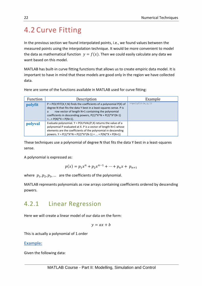
Here are some of the functions available in MATLAB used for curve fitting:
Function Description Example
polyfit P = POLYFIT(X,Y,N) finds the coefficients of a polynomial P(X) of degree N that fits the data Y best in a least-squares sense. P is a row vector of length N+1 containing the polynomial coefficients in descending powers, P(1)*X^N + P(2)*X^(N-1) +...+ P(N)*X + P(N+1).
>>polyfit(x,y,1)
polyval Evaluate polynomial. Y = POLYVAL(P,X) returns the value of a polynomial P evaluated at X. P is a vector of length N+1 whose elements are the coefficients of the polynomial in descending powers. Y = P(1)*X^N + P(2)*X^(N-1) + ... + P(N)*X + P(N+1)
These techniques use a polynomial of degree N that fits the data Y best in a least-squares
sense.
A polynomial is expressed as:
𝑝(𝑥) = 𝑝1𝑥𝑛 + 𝑝2𝑥
𝑛−1 +⋯+ 𝑝𝑛𝑥 + 𝑝𝑛+1
where 𝑝1, 𝑝2, 𝑝3, … are the coefficients of the polynomial.
MATLAB represents polynomials as row arrays containing coefficients ordered by descending
powers.
4.2.1 Linear Regression
Here we will create a linear model of our data on the form:
𝑦 = 𝑎𝑥 + 𝑏
This is actually a polynomial of 1.order
Example:
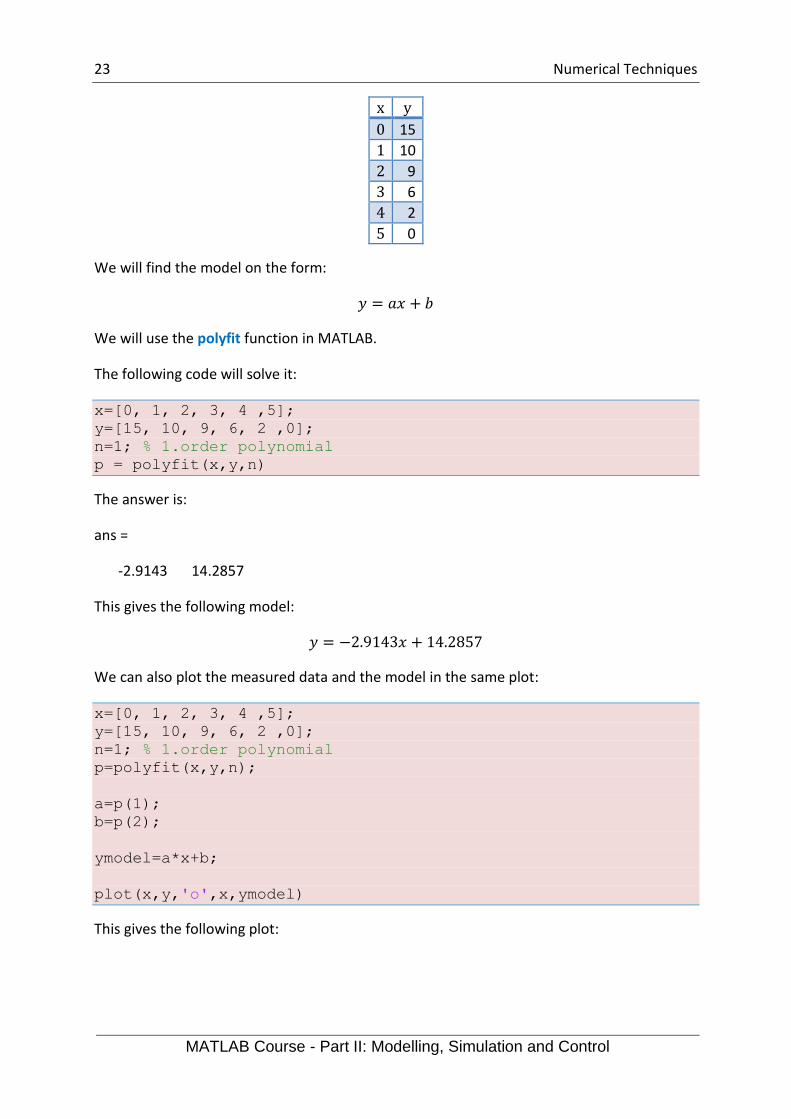
Given the following data:
23 Numerical Techniques
MATLAB Course - Part II: Modelling, Simulation and Control
x y
0 15
1 10
2 9
3 6
4 2
5 0
We will find the model on the form:
𝑦 = 𝑎𝑥 + 𝑏
We will use the polyfit function in MATLAB.
The following code will solve it:
x=[0, 1, 2, 3, 4 ,5];
y=[15, 10, 9, 6, 2 ,0];
n=1; % 1.order polynomial
p = polyfit(x,y,n)
The answer is:
ans =
-2.9143 14.2857
This gives the following model:
𝑦 = −2.9143𝑥 + 14.2857
We can also plot the measured data and the model in the same plot:
x=[0, 1, 2, 3, 4 ,5];
y=[15, 10, 9, 6, 2 ,0];
n=1; % 1.order polynomial
p=polyfit(x,y,n);
a=p(1);
b=p(2);
ymodel=a*x+b;
plot(x,y,'o',x,ymodel)
This gives the following plot:

24 Numerical Techniques
MATLAB Course - Part II: Modelling, Simulation and Control
We see this gives a good model based on the data available.
[End of Example]
Task 9: Linear Regression
Given the following data:
Temperature, T [ oC] Energy, u [KJ/kg]
100 2506.7
150 2582.8
200 2658.1
250 2733.7
300 2810.4
400 2967.9
500 3131.6
Plot u versus T.
Find the linear regression model from the data
𝑦 = 𝑎𝑥 + 𝑏
Plot it in the same graph.
[End of Task]

25 Numerical Techniques
MATLAB Course - Part II: Modelling, Simulation and Control
4.2.2 Polynomial Regression
In the previous section we used linear regression which is a 1.order polynomial. In this
section we will study higher order polynomials.
In polynomial regression we will find the following model:
𝑦(𝑥) = 𝑎0𝑥𝑛 + 𝑎1𝑥
𝑛−1 +⋯+ 𝑎𝑛−1𝑥 + 𝑎𝑛
Example:
Given the following data:
x y
0 15
1 10
2 9
3 6
4 2
5 0
We will found the model of the form:
𝑦(𝑥) = 𝑎0𝑥𝑛 + 𝑎1𝑥
𝑛−1 +⋯+ 𝑎𝑛−1𝑥 + 𝑎𝑛
We will use the polyfit and polyval functions in MATLAB and compare the models using
different orders of the polynomial.
We will investigate models of 2.order, 3.order, 4.order and 5.order. We have only 6 data
points, so a model with order higher than 5 will make no sense.
We use a For loop in order to create models of 2, 3, 4 and 5.order.
The code is as follows:
x=[0, 1, 2, 3, 4 ,5];
y=[15, 10, 9, 6, 2 ,0];
for n=2:5 %From order 2 to 5
p=polyfit(x,y,n)
ymodel=polyval(p,x);
subplot(2,2,n-1)
plot(x,y,'o',x,ymodel)
title(sprintf('Model of order %d', n));
end
26 Numerical Techniques
MATLAB Course - Part II: Modelling, Simulation and Control
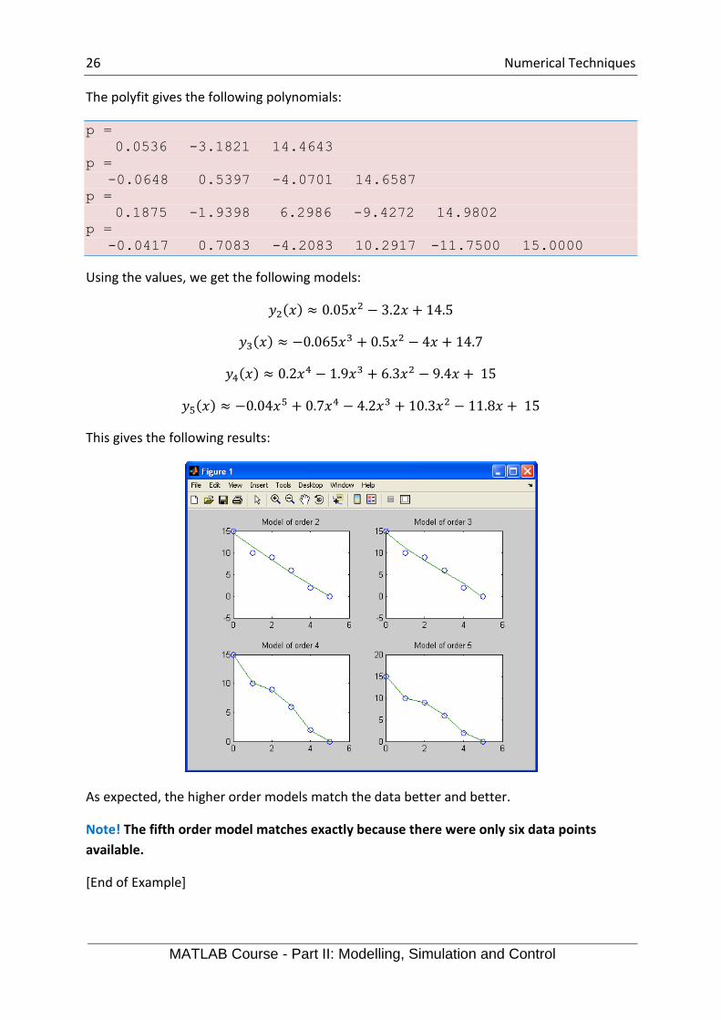
The polyfit gives the following polynomials:
p =
0.0536 -3.1821 14.4643
p =
-0.0648 0.5397 -4.0701 14.6587
p =
0.1875 -1.9398 6.2986 -9.4272 14.9802
p =
-0.0417 0.7083 -4.2083 10.2917 -11.7500 15.0000
Using the values, we get the following models:
𝑦2(𝑥) ≈ 0.05𝑥2 − 3.2𝑥 + 14.5
𝑦3(𝑥) ≈ −0.065𝑥3 + 0.5𝑥2 − 4𝑥 + 14.7
𝑦4(𝑥) ≈ 0.2𝑥4 − 1.9𝑥3 + 6.3𝑥2 − 9.4𝑥 + 15
𝑦5(𝑥) ≈ −0.04𝑥5 + 0.7𝑥4 − 4.2𝑥3 + 10.3𝑥2 − 11.8𝑥 + 15
This gives the following results:
As expected, the higher order models match the data better and better.
Note! The fifth order model matches exactly because there were only six data points
available.
[End of Example]
27 Numerical Techniques
MATLAB Course - Part II: Modelling, Simulation and Control
Task 10: Polynomial Regression
Given the following data:
x y
10 23
20 45
30 60
40 82
50 111
60 140
70 167
80 198
90 200
100 220
→ Use the polyfit and polyval functions in MATLAB and compare the models using different
orders of the polynomial.
Use subplots and make sure to add titles, etc.
[End of Task]
Task 11: Model fitting
Given the following data:
Height, h[ft] Flow, f[ft^3/s]
0 0
1.7 2.6
1.95 3.6
2.60 4.03
2.92 6.45
4.04 11.22
5.24 30.61
→ Create a 1. (linear), 2. (quadratic) and 3.order (cubic) model. Which gives the best model?
Plot the result in the same plot and compare them. Add xlabel, ylabel, title and a legend to
the plot and use different line styles so the user can easily see the difference.
[End of Task]
4.3 Numerical Differentiation
28 Numerical Techniques
MATLAB Course - Part II: Modelling, Simulation and Control
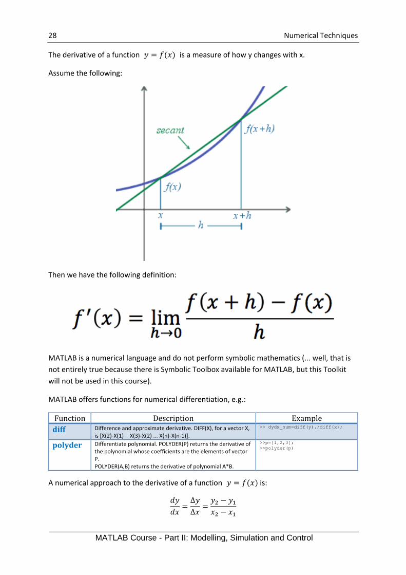
The derivative of a function 𝑦 = 𝑓(𝑥) is a measure of how y changes with x.
Assume the following:
Then we have the following definition:
MATLAB is a numerical language and do not perform symbolic mathematics (... well, that is
not entirely true because there is Symbolic Toolbox available for MATLAB, but this Toolkit
will not be used in this course).
MATLAB offers functions for numerical differentiation, e.g.:
Function Description Example
diff Difference and approximate derivative. DIFF(X), for a vector X, is [X(2)-X(1) X(3)-X(2) ... X(n)-X(n-1)].
>> dydx_num=diff(y)./diff(x);
polyder Differentiate polynomial. POLYDER(P) returns the derivative of the polynomial whose coefficients are the elements of vector P. POLYDER(A,B) returns the derivative of polynomial A*B.
>>p=[1,2,3];
>>polyder(p)
A numerical approach to the derivative of a function 𝑦 = 𝑓(𝑥) is:
𝑑𝑦
𝑑𝑥=∆𝑦
∆𝑥=𝑦2 − 𝑦1𝑥2 − 𝑥1

29 Numerical Techniques
MATLAB Course - Part II: Modelling, Simulation and Control
This approximation of the derivative corresponds to the slope of each line segment used to
connect each data point that exists. An example is shown below:
Example:
We will use Numerical Differentiation to find 𝑑𝑦
𝑑𝑥 on the following function:
𝑦 = 𝑥2
based on the data points (x=-2:2):
x y
-2 4
-1 1
0 0
1 1
2 4
First, we will plot the data points together with the real function 𝑦 = 𝑥2 using the following
code:
x=-2:0.1:2;
y=x.^2;
plot(x,y)
hold on
x=-2:2;
y=x.^2;
plot(x,y, '-oc')
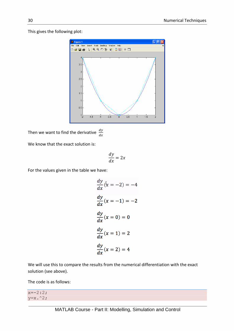
30 Numerical Techniques
MATLAB Course - Part II: Modelling, Simulation and Control
This gives the following plot:
Then we want to find the derivative 𝑑𝑦
𝑑𝑥
We know that the exact solution is:
𝑑𝑦
𝑑𝑥= 2𝑥
For the values given in the table we have:
We will use this to compare the results from the numerical differentiation with the exact
solution (see above).
The code is as follows:
x=-2:2;
y=x.^2;

31 Numerical Techniques
MATLAB Course - Part II: Modelling, Simulation and Control
dydx_num=diff(y)./diff(x);
dydx_exact=2*x;
dydx=[[dydx_num, NaN]', dydx_exact']
This gives the following results (left column is from the numerical derivation, while the right
column is from the exact derivation):
dydx =
-3 -4
-1 -2
1 0
3 2
NaN 4
Note! NaN is added to the vector with numerical differentiation in order to get the same
length of the vectors.
If we plot the derivatives (numerical and exact), we get:
If we increase the number of data points (x=-2:0.1:2) we get a better result:

32 Numerical Techniques
MATLAB Course - Part II: Modelling, Simulation and Control
[End of Example]
Task 12: Numerical Differentiation
Given the following equation:
𝑦 = 𝑥3 + 2𝑥2 − 𝑥 + 3
Find 𝑑𝑦
𝑑𝑥 analytically (use “pen and paper”).
Define a vector x from -5 to +5 and use the diff function to approximate the derivative y with
respect to x (∆𝑦
∆𝑥).
Compare the data in a 2D array and/or plot both the exact value of 𝑑𝑦
𝑑𝑥 and the
approximation in the same plot.
Increase number of data point to see if there are any difference.
Do the same for the following functions:
𝑦 = sin (𝑥)
𝑦 = 𝑥5 − 1
[End of Task]
4.3.1 Differentiation on Polynomials

33 Numerical Techniques
MATLAB Course - Part II: Modelling, Simulation and Control
A polynomial is expressed as:
𝑝(𝑥) = 𝑝1𝑥𝑛 + 𝑝2𝑥
𝑛−1 +⋯+ 𝑝𝑛𝑥 + 𝑝𝑛+1
where 𝑝1, 𝑝2, 𝑝3, … are the coefficients of the polynomial.
The differentiation of the Polynomial will be:
𝑝(𝑥)′ = 𝑝1𝑛𝑥𝑛−1 + 𝑝2(𝑛 − 1)𝑥
𝑛−2 +⋯+ 𝑝𝑛
Example
Given the polynomial
𝑝(𝑥) = 2 + 𝑥3
We can rewrite the polynomial like this:
𝑝(𝑥) = 1 ∙ 𝑥3 + 0 ∙ 𝑥2 + 0 ∙ 𝑥 + 2
The polynomial is defined in MATLAB as:
>> p=[1, 0, 0, 2]
We know that: 𝑝′ = 3𝑥2
The code is as follows
>> p=[1, 0, 0, 2]
p =
1 0 0 2
>> polyder(p)
ans =
3 0 0
Which is correct, because
𝑝(𝑥)′ = 3 ∙ 𝑥2 + 0 ∙ 𝑥2 + 0
with the coefficients:
𝑝1 = 3, 𝑝2 = 0, 𝑝3 = 0
And this is written as a vector [3 0 0] in MATLAB.
[End of Example]
Task 13: Differentiation on Polynomials

34 Numerical Techniques
MATLAB Course - Part II: Modelling, Simulation and Control
Consider the following equation:
𝑦 = 𝑥3 + 2𝑥2 − 𝑥 + 3
Use Differentiation on the Polynomial to find 𝑑𝑦
𝑑𝑥
[End of Task]
Task 14: Differentiation on Polynomials
Find the derivative for the product:
(3𝑥2 + 6𝑥 + 9)(𝑥2 + 2𝑥)
Use the polyder(a,b) function.
Another approach is to use define is to first use the conv(a,b) function to find the total
polynomial, and then use polyder(p) function.
Try both methods, to see if you get the same answer.
[End of Task]
4.4 Numerical Integration
The integral of a function 𝑓(𝑥) is denoted as:
∫ 𝑓(𝑥)𝑑𝑥𝑏
𝑎
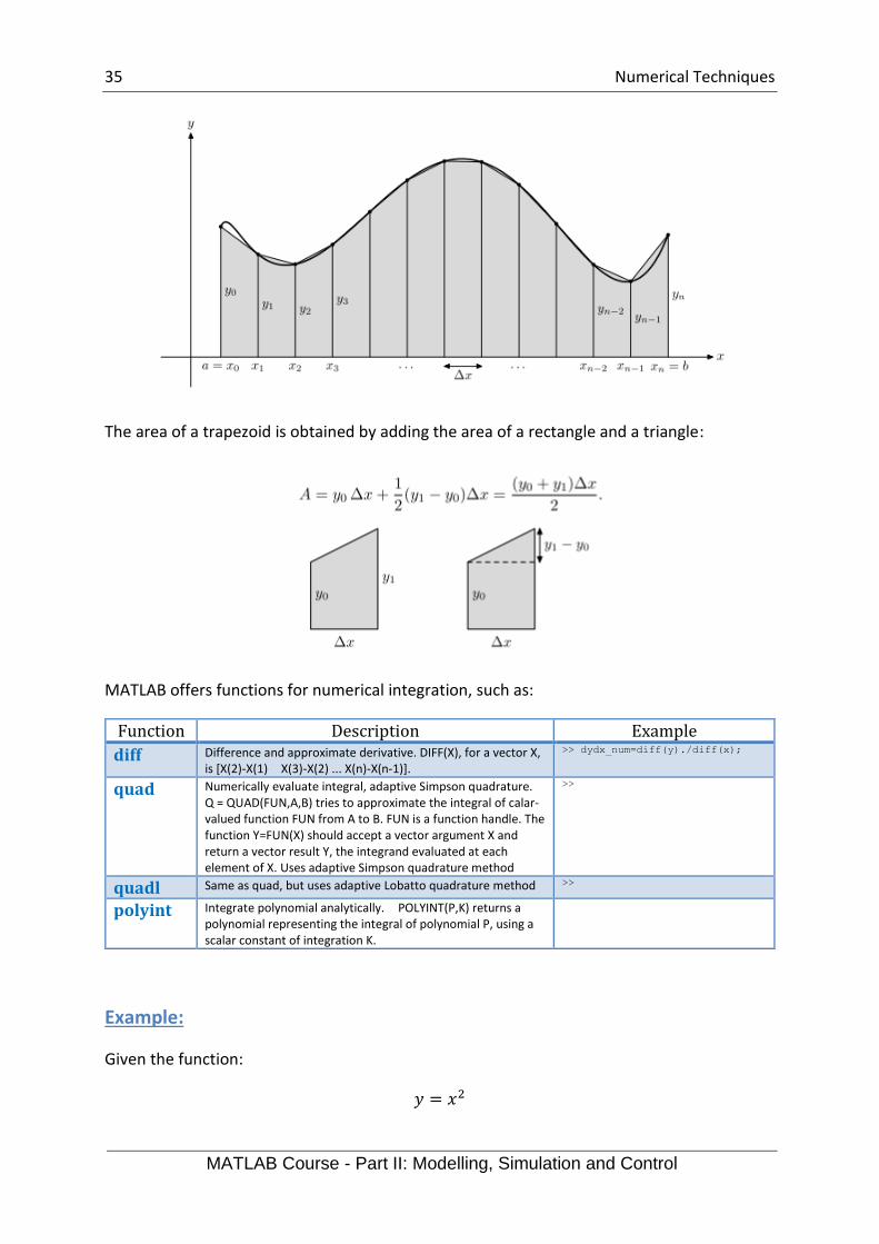
An integral can be seen as the area under a curve. Given 𝑦 = 𝑓(𝑥) the approximation of
the Area (A) under the curve can be found dividing the area up into rectangles and then
summing the contribution from all the rectangles:
𝐴 = ∑(𝑥𝑖+1 − 𝑥𝑖) ∙ (𝑦𝑖+1 + 𝑦𝑖)/2
𝑛−1
𝑖=1
This is known as the trapezoid rule.
We approximate the integral by using n trapezoids formed by using straight line segments
between the points (𝑥𝑖−1, 𝑦𝑖−1) and (𝑥𝑖, 𝑦𝑖) for 1 ≤ 𝑖 ≤ 𝑛 as shown in the figure below:
35 Numerical Techniques
MATLAB Course - Part II: Modelling, Simulation and Control
The area of a trapezoid is obtained by adding the area of a rectangle and a triangle:
MATLAB offers functions for numerical integration, such as:
Function Description Example
diff Difference and approximate derivative. DIFF(X), for a vector X, is [X(2)-X(1) X(3)-X(2) ... X(n)-X(n-1)].
>> dydx_num=diff(y)./diff(x);
quad Numerically evaluate integral, adaptive Simpson quadrature. Q = QUAD(FUN,A,B) tries to approximate the integral of calar-valued function FUN from A to B. FUN is a function handle. The function Y=FUN(X) should accept a vector argument X and return a vector result Y, the integrand evaluated at each element of X. Uses adaptive Simpson quadrature method
>>
quadl Same as quad, but uses adaptive Lobatto quadrature method >>
polyint Integrate polynomial analytically. POLYINT(P,K) returns a polynomial representing the integral of polynomial P, using a scalar constant of integration K.
Example:
Given the function:
𝑦 = 𝑥2

36 Numerical Techniques
MATLAB Course - Part II: Modelling, Simulation and Control
We know that the exact solution is:
∫ 𝑥2𝑑𝑥 =𝑎3
3
𝑎
0
The integral from 0 to 1 is:
∫ 𝑥2𝑑𝑥 =1
3
1
0
≈ 0.3333
We will use the trapezoid rule and the diff function in MATLAB to solve the numerical
integral of 𝑥2 from 0 to 1.
The MATLAB code for this is:
x=0:0.1:1;
y=x.^2;
avg_y = y(1:length(x)-1) + diff(y)/2;
A = sum(diff(x).*avg_y)
Note!
The following two lines of code
avg_y = y(1:length(x)-1) + diff(y)/2;
A = sum(diff(x).*avg_y)
Implements this formula, known as the trapezoid rule:
𝐴 = ∑(𝑥𝑖+1 − 𝑥𝑖) ∙ (𝑦𝑖+1 + 𝑦𝑖)/2
𝑛−1
𝑖=1
37 Numerical Techniques
MATLAB Course - Part II: Modelling, Simulation and Control
The result from the approximation is:
A =
0.3350
If we use the functions quad we get:
quad('x.^2', 0,1)
ans =
0.3333
If we use the functions quadl we get:
quadl('x.^2', 0,1)
ans =
0.3333
[End of Example]
Task 15: Numerical Integration
Use diff, quad and quadl on the following equation:
𝑦 = 𝑥3 + 2𝑥2 − 𝑥 + 3
Find the integral of y with respect to x, evaluated from -1 to 1
Compare the different methods.
The exact solution is:
∫ (𝑥3 + 2𝑥2 − 𝑥 + 3)𝑑𝑥𝑏
𝑎
= (𝑥4
4+2𝑥3
3−𝑥2
2+ 3𝑥)|
𝑎
𝑏
=1
4(𝑏4 − 𝑎4) +
2
3(𝑏3 − 𝑎3) −
1
2(𝑏2 − 𝑎2) + 3(𝑏 − 𝑎)
Compare the result with the exact solution.
Repeat the task for the following functions:
𝑦 = sin(𝑥)
𝑦 = 𝑥5 − 1
[End of Task]

38 Numerical Techniques
MATLAB Course - Part II: Modelling, Simulation and Control
4.4.1 Integration on Polynomials
A polynomial is expressed as:
𝑝(𝑥) = 𝑝1𝑥𝑛 + 𝑝2𝑥
𝑛−1 +⋯+ 𝑝𝑛𝑥 + 𝑝𝑛+1
where 𝑝1, 𝑝2, 𝑝3, … are the coefficients of the polynomial.
In MATLAB we can use the polyint function to perform integration on polynomials. This
function works the same way as the polyder function which performs differentiation on
polynomials.
Task 16: Integration on Polynomials
Consider the following equation:
𝑦 = 𝑥3 + 2𝑥2 − 𝑥 + 3
Find the integral of 𝑦 with respect to 𝑥 (∫ 𝑦𝑑𝑥) using MATLAB.
[End of Task]
39
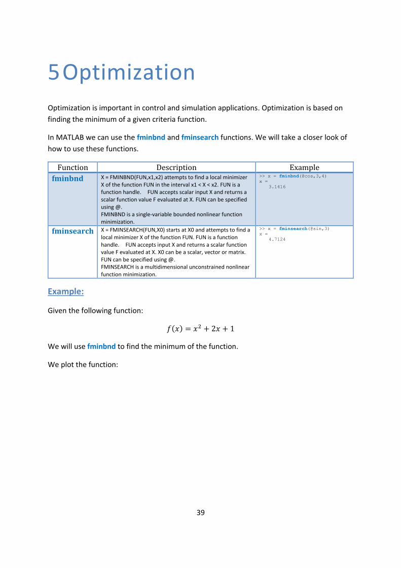
5 Optimization
Optimization is important in control and simulation applications. Optimization is based on
finding the minimum of a given criteria function.
In MATLAB we can use the fminbnd and fminsearch functions. We will take a closer look of
how to use these functions.
Function Description Example
fminbnd X = FMINBND(FUN,x1,x2) attempts to find a local minimizer X of the function FUN in the interval x1 < X < x2. FUN is a function handle. FUN accepts scalar input X and returns a scalar function value F evaluated at X. FUN can be specified using @. FMINBND is a single-variable bounded nonlinear function minimization.
>> x = fminbnd(@cos,3,4)
x =
3.1416
fminsearch X = FMINSEARCH(FUN,X0) starts at X0 and attempts to find a local minimizer X of the function FUN. FUN is a function handle. FUN accepts input X and returns a scalar function value F evaluated at X. X0 can be a scalar, vector or matrix. FUN can be specified using @. FMINSEARCH is a multidimensional unconstrained nonlinear function minimization.
>> x = fminsearch(@sin,3)
x =
4.7124
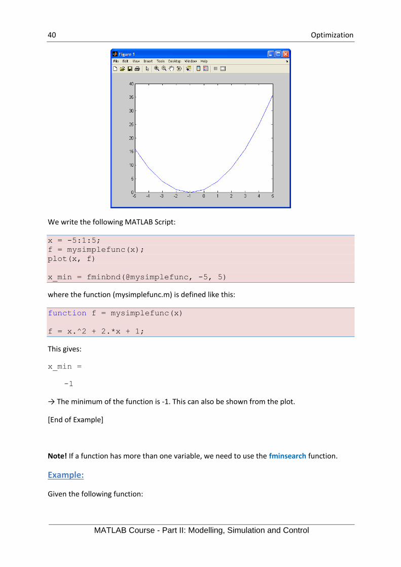
Example:
Given the following function:
𝑓(𝑥) = 𝑥2 + 2𝑥 + 1
We will use fminbnd to find the minimum of the function.
We plot the function:
40 Optimization
MATLAB Course - Part II: Modelling, Simulation and Control
We write the following MATLAB Script:
x = -5:1:5;
f = mysimplefunc(x);
plot(x, f)
x_min = fminbnd(@mysimplefunc, -5, 5)
where the function (mysimplefunc.m) is defined like this:
function f = mysimplefunc(x)
f = x.^2 + 2.*x + 1;
This gives:
x_min =
-1
→ The minimum of the function is -1. This can also be shown from the plot.
[End of Example]
Note! If a function has more than one variable, we need to use the fminsearch function.
Example:
Given the following function:

41 Optimization
MATLAB Course - Part II: Modelling, Simulation and Control
𝑓(𝑥, 𝑦) = 2(𝑥 − 1)2 + 𝑥 − 2 + (𝑦 − 2)2 + 𝑦
We will use fminsearch to find the minimum of the function.
The MATLAB Code can be written like this:
[x,fval] = fminsearch(@myfunc, [1;1])
where the function is defined like this:
function f = myfunc(x)
f = 2*(x(1)-1).^2 + x(1) - 2 + (x(2)-2).^2 + x(2);
Note! The unknowns x and y is defined as a vector, i.e., 𝑥1 = 𝑥(1) = 𝑥, 𝑥2 = 𝑥(2) = 𝑦.
𝑥 = [𝑥1𝑥2]
If there is more than one variable, you have to do it this way.
This gives:
x =
0.7500
1.5000
fval =
0.6250
→ The minimum is of the function is given by 𝑥 = 0.75 and 𝑦 = 1.5.
We can also plot the function:
clear,clc
[x,y] = meshgrid(-2:0.1:2, -1:0.1:3);
f = 2.*(x-1).^2 + x - 2 + (y-2).^2 + y;
figure(1)
surf(x,y,f)
figure(2)
mesh(x,y,f)
figure(3)
surfl(x,y,f)
shading interp;
colormap(hot);
For figure 3 we get:
42 Optimization
MATLAB Course - Part II: Modelling, Simulation and Control
[End of Example]
Task 17: Optimization
Given the following function:
𝑓(𝑥) = 𝑥3 − 4𝑥
→ Plot the function
→ Find the minimum for this function
[End of Task]
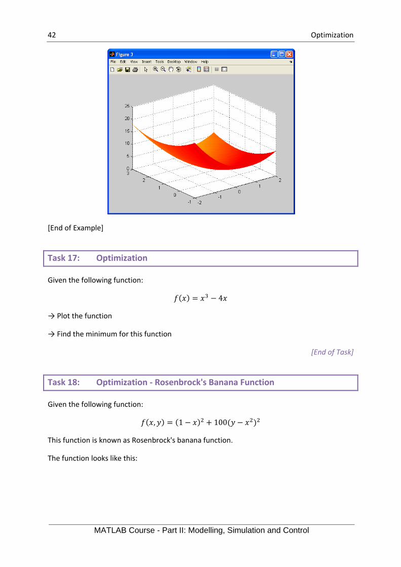
Task 18: Optimization - Rosenbrock's Banana Function
Given the following function:
𝑓(𝑥, 𝑦) = (1 − 𝑥)2 + 100(𝑦 − 𝑥2)2
This function is known as Rosenbrock's banana function.
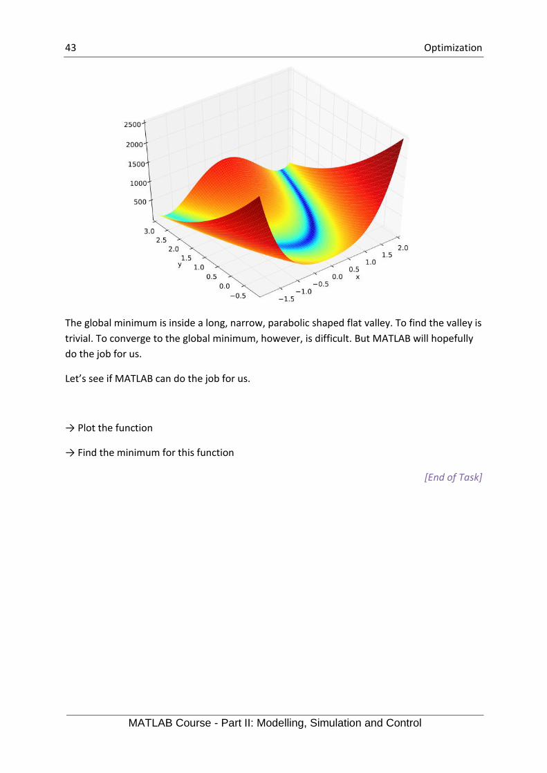
The function looks like this:
43 Optimization
MATLAB Course - Part II: Modelling, Simulation and Control
The global minimum is inside a long, narrow, parabolic shaped flat valley. To find the valley is
trivial. To converge to the global minimum, however, is difficult. But MATLAB will hopefully
do the job for us.
Let’s see if MATLAB can do the job for us.
→ Plot the function
→ Find the minimum for this function
[End of Task]
44
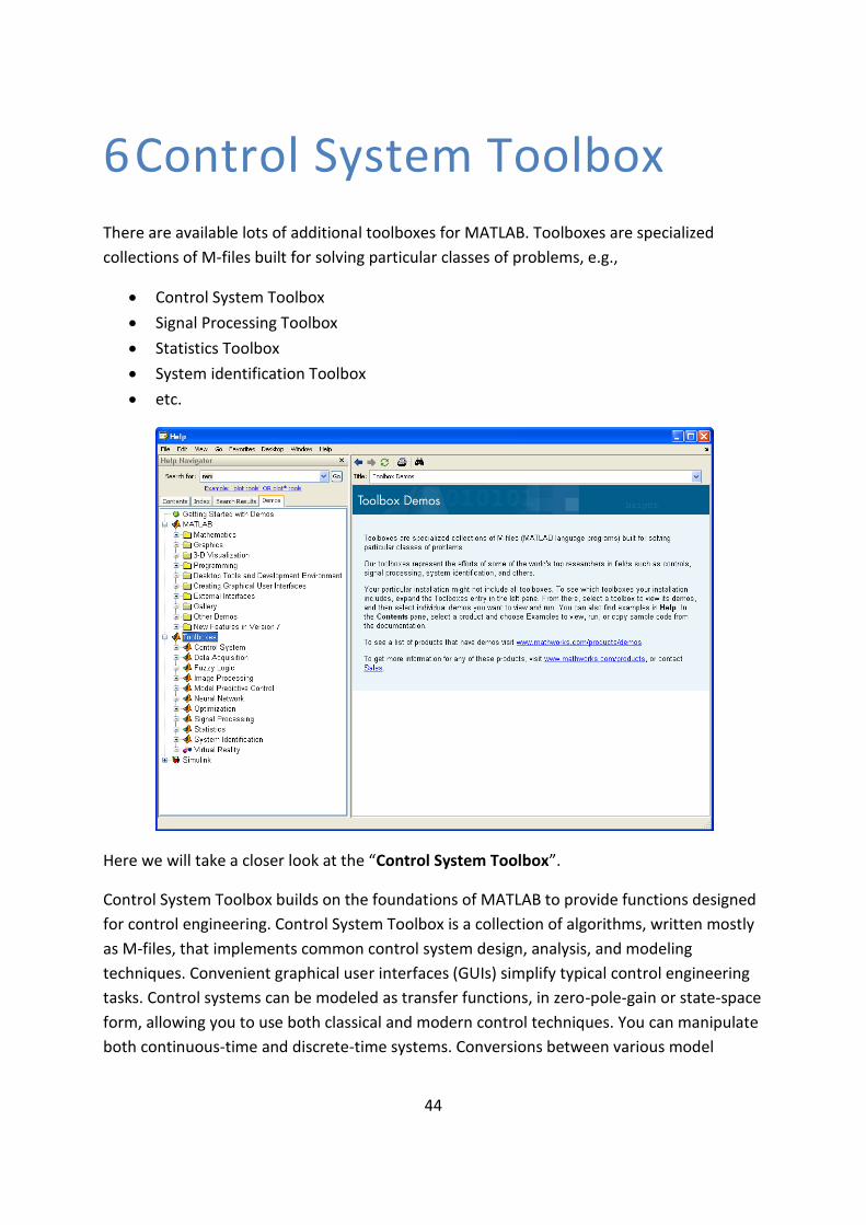
6 Control System Toolbox
There are available lots of additional toolboxes for MATLAB. Toolboxes are specialized
collections of M-files built for solving particular classes of problems, e.g.,
• Control System Toolbox
• Signal Processing Toolbox
• Statistics Toolbox
• System identification Toolbox
• etc.
Here we will take a closer look at the “Control System Toolbox”.
Control System Toolbox builds on the foundations of MATLAB to provide functions designed
for control engineering. Control System Toolbox is a collection of algorithms, written mostly
as M-files, that implements common control system design, analysis, and modeling
techniques. Convenient graphical user interfaces (GUIs) simplify typical control engineering
tasks. Control systems can be modeled as transfer functions, in zero-pole-gain or state-space
form, allowing you to use both classical and modern control techniques. You can manipulate
both continuous-time and discrete-time systems. Conversions between various model
45 Control System Toolbox
MATLAB Course - Part II: Modelling, Simulation and Control
representations are provided. Time responses, frequency responses can be computed and
graphed. Other functions allow pole placement, optimal control, and estimation. Finally,
Control System Toolbox is open and extensible. You can create custom M-files to suit your
particular application.
46
7 Transfer Functions
It is assumed you are familiar with basic control theory and transfer functions, if not you may
skip this chapter.
7.1 Introduction
Transfer functions are a model form based on the Laplace transform. Transfer functions are
very useful in analysis and design of linear dynamic systems.
A general transfer function is on the form:
𝐻(𝑆) =𝑦(𝑠)
𝑢(𝑠)
Where 𝑦 is the output and 𝑢 is the input.
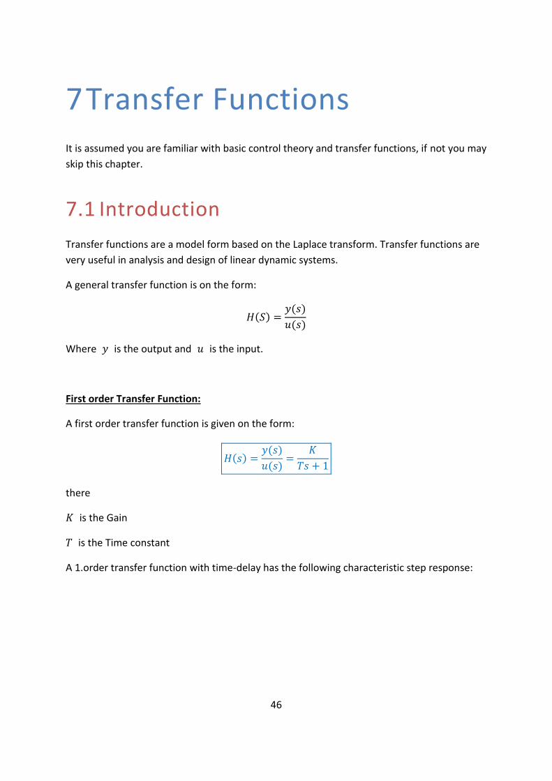
First order Transfer Function:
A first order transfer function is given on the form:
𝐻(𝑠) =𝑦(𝑠)
𝑢(𝑠)=
𝐾
𝑇𝑠 + 1
there
𝐾 is the Gain
𝑇 is the Time constant
A 1.order transfer function with time-delay has the following characteristic step response:
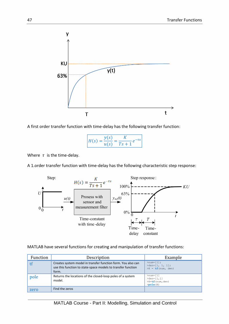
47 Transfer Functions
MATLAB Course - Part II: Modelling, Simulation and Control
A first order transfer function with time-delay has the following transfer function:
𝐻(𝑠) =𝑦(𝑠)
𝑢(𝑠)=
𝐾
𝑇𝑠 + 1𝑒−𝜏𝑠
Where 𝜏 is the time-delay.
A 1.order transfer function with time-delay has the following characteristic step response:
MATLAB have several functions for creating and manipulation of transfer functions:
Function Description Example
tf Creates system model in transfer function form. You also can use this function to state-space models to transfer function form.
>num=[1];
>den=[1, 1, 1];
>H = tf(num, den)
pole Returns the locations of the closed-loop poles of a system model.
>num=[1]
>den=[1,1]
>H=tf(num,den)
>pole(H)
zero Find the zeros

48 Transfer Functions
MATLAB Course - Part II: Modelling, Simulation and Control
step Creates a step response plot of the system model. You also can use this function to return the step response of the model outputs. If the model is in state-space form, you also can use this function to return the step response of the model states. This function assumes the initial model states are zero. If you do not specify an output, this function creates a plot.
>num=[1,1];
>den=[1,-1,3];
>H=tf(num,den);
>t=[0:0.01:10];
>step(H,t);
lsim Creates the linear simulation plot of a system model. This function calculates the output of a system model when a set of inputs excite the model, using discrete simulation. If you do not specify an output, this function creates a plot.
>t = [0:0.1:10]
>u = sin(0.1*pi*t)'
>lsim(SysIn, u, t)
conv Computes the convolution of two vectors or matrices. >C1 = [1, 2, 3];
>C2 = [3, 4];
>C = conv(C1, C2)
series Connects two system models in series to produce a model SysSer with input and output connections you specify
>Hseries = series(H1,H2)
feedback Connects two system models together to produce a closed-loop model using negative or positive feedback connections
>SysClosed = feedback(SysIn_1,
SysIn_2)
c2d Convert from continuous- to discrete-time models
d2c Convert from discrete- to continuous-time models
Before you start, you should use the Help system in MATLAB to read more about these
functions. Type “help <functionname>” in the Command window.
Task 19: Transfer function
Use the tf function in MATLAB to define the transfer function above. Set 𝐾 = 2 and 𝑇 = 3.
Type “help tf” in the Command window to see how you use this function.
Example:
% Transfer function H=1/(s+1)
num = [1];
den = [1, 1];
H = tf(num, den)
[End of Task]
7.2 Second order Transfer Function
A second order transfer function is given on the form:
𝐻(𝑠) =𝐾
(𝑠𝜔0)2
+ 2𝜁𝑠𝜔0+ 1
Where
𝐾 is the gain

49 Transfer Functions
MATLAB Course - Part II: Modelling, Simulation and Control
𝜁 zeta is the relative damping factor
𝜔0[rad/s] is the undamped resonance frequency.
Task 20: 2.order Transfer function
Define the transfer function using the tf function.
Set 𝐾 = 1,𝜔0 = 1
→ Plot the step response (use the step function in MATLAB) for different values of 𝜁. Select
𝜁 as follows:
𝜁 > 1
𝜁 = 1
0 < 𝜁 < 1
𝜁 = 0
𝜁 < 0
Tip! From control theory we have the following:
Figure: F. Haugen, Advanced Dynamics and Control: TechTeach, 2010.

50 Transfer Functions
MATLAB Course - Part II: Modelling, Simulation and Control
So you should get similar step responses as shown above.
[End of Task]
Task 21: Time Response
Given the following system:
𝐻(𝑠) =𝑠 + 1
𝑠2 − 𝑠 + 3
Plot the time response for the transfer function using the step function. Let the time-interval
be from 0 to 10 seconds, e.g., define the time vector like this:
t=[0:0.01:10]
and then use the function step(H,t).
[End of Task]
7.3 Analysis of Standard Functions
Here we will take a closer look at the following standard functions:
• Integrator
• 1. Order system
• 2. Order system
Task 22: Integrator
The transfer function for an Integrator is as follows:
𝐻(𝑠) =𝐾
𝑠
→Find the pole(s)
→ Plot the Step response: Use different values for 𝐾, e.g., 𝐾 = 0.2, 1, 5. Use the step
function in MATLAB.
[End of Task]
51 Transfer Functions
MATLAB Course - Part II: Modelling, Simulation and Control
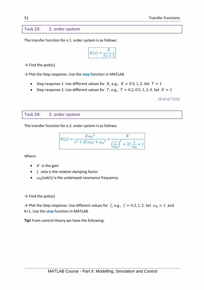
Task 23: 1. order system
The transfer function for a 1. order system is as follows:
𝐻(𝑠) =𝐾
𝑇𝑠 + 1
→ Find the pole(s)
→ Plot the Step response. Use the step function in MATLAB.
• Step response 1: Use different values for 𝐾, e.g., 𝐾 = 0.5, 1, 2. Set 𝑇 = 1
• Step response 2: Use different values for 𝑇, e.g., 𝑇 = 0.2, 0.5, 1, 2, 4. Set 𝐾 = 1
[End of Task]
Task 24: 2. order system
The transfer function for a 2. order system is as follows:
𝐻(𝑠) =𝐾𝜔0
2
𝑠2 + 2𝜁𝜔0𝑠 + 𝜔02=
𝐾
(𝑠𝜔0)2
+ 2𝜁𝑠𝜔0+ 1
Where
• 𝐾 is the gain
• 𝜁 zeta is the relative damping factor
• 𝜔0[rad/s] is the undamped resonance frequency.
→ Find the pole(s)
→ Plot the Step response: Use different values for 𝜁, e.g., 𝜁 = 0.2, 1, 2. Set 𝜔0 = 1 and
K=1. Use the step function in MATLAB.
Tip! From control theory we have the following:

52 Transfer Functions
MATLAB Course - Part II: Modelling, Simulation and Control
Figure: F. Haugen, Advanced Dynamics and Control: TechTeach, 2010.
So you should get similar step responses as shown above.
[End of Task]
Task 25: 2. order system – Special Case
Special case: When 𝜻 > 0 and the poles are real and distinct we have:
𝐻(𝑠) =𝐾
(𝑇1𝑠 + 1)(𝑇2𝑠 + 1)
We see that this system can be considered as two 1.order systems in series.
𝐻(𝑠) = 𝐻1(𝑠)𝐻1(𝑠) =𝐾
(𝑇1𝑠 + 1)∙
1
(𝑇2𝑠 + 1)=
𝐾
(𝑇1𝑠 + 1)(𝑇2𝑠 + 1)
53 Transfer Functions
MATLAB Course - Part II: Modelling, Simulation and Control
Set 𝑇1 = 2 and 𝑇2 = 5
→ Find the pole(s)
→ Plot the Step response. Set K=1. Set 𝑇1 = 1 𝑎𝑛𝑑 𝑇2 = 0, 𝑇1 = 1 𝑎𝑛𝑑 𝑇2 = 0.05, 𝑇1 =
1 𝑎𝑛𝑑 𝑇2 = 0.1, 𝑇1 = 1 𝑎𝑛𝑑 𝑇2 = 0.25, 𝑇1 = 1 𝑎𝑛𝑑 𝑇2 = 0.5, 𝑇1 = 1 𝑎𝑛𝑑 𝑇2 = 1. Use the
step function in MATLAB.
[End of Task]
54
8 State-space Models
It is assumed you are familiar with basic control theory and state-space models, if not you
may skip this chapter.
8.1 Introduction
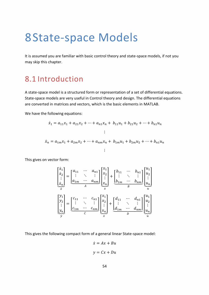
A state-space model is a structured form or representation of a set of differential equations.
State-space models are very useful in Control theory and design. The differential equations
are converted in matrices and vectors, which is the basic elements in MATLAB.
We have the following equations:
�̇�1 = 𝑎11𝑥1 + 𝑎21𝑥2 +⋯+ 𝑎𝑛1𝑥𝑛 + 𝑏11𝑢1 + 𝑏21𝑢2 +⋯+ 𝑏𝑛1𝑢𝑛
⋮
�̇�𝑛 = 𝑎1𝑚𝑥1 + 𝑎2𝑚𝑥2 +⋯+ 𝑎𝑛𝑚𝑥𝑛 + 𝑏1𝑚𝑢1 + 𝑏2𝑚𝑢2 +⋯+ 𝑏𝑛1𝑢𝑛
⋮
This gives on vector form:
[
�̇�1�̇�2⋮�̇�𝑛
]
⏟�̇�
= [
𝑎11 ⋯ 𝑎𝑛1⋮ ⋱ ⋮𝑎1𝑚 ⋯ 𝑎𝑛𝑚
]⏟
𝐴
[
𝑥1𝑥2⋮𝑥𝑛
]
⏟𝑥
+ [𝑏11 ⋯ 𝑏𝑛1⋮ ⋱ ⋮𝑏1𝑚 ⋯ 𝑏𝑛𝑚
]⏟
𝐵
[
𝑢1𝑢2⋮𝑢𝑛
]
⏟𝑢
[
𝑦1𝑦2⋮𝑦𝑛
]
⏟𝑦
= [
𝑐11 ⋯ 𝑐𝑛1⋮ ⋱ ⋮𝑐1𝑚 ⋯ 𝑐𝑛𝑚
]⏟
𝐶
[
𝑥1𝑥2⋮𝑥𝑛
]
⏟𝑥
+ [𝑑11 ⋯ 𝑑𝑛1⋮ ⋱ ⋮𝑑1𝑚 ⋯ 𝑑𝑛𝑚
]⏟
𝐷
[
𝑢1𝑢2⋮𝑢𝑛
]
⏟𝑢
This gives the following compact form of a general linear State-space model:
�̇� = 𝐴𝑥 + 𝐵𝑢
𝑦 = 𝐶𝑥 + 𝐷𝑢

55 State-space Models
MATLAB Course - Part II: Modelling, Simulation and Control
Example:
Given the following equations:
�̇�1 = −1
𝐴𝑡𝑥2 +
1
𝐴𝑡𝐾𝑝𝑢
�̇�2 = 0
These equations can be written on the compact state-space form:
[�̇�1�̇�2] = [
0 −1
𝐴𝑡0 0
]
⏟ 𝐴
[𝑥1𝑥2] + [
𝐾𝑝
𝐴𝑡0
]
⏟𝐵
𝑢
𝑦 = [1 0]⏟ 𝐶
[𝑥1𝑥2]
[End of Example]
MATLAB have several functions for creating and manipulation of State-space models:
Function Description Example
ss Constructs a model in state-space form. You also can use this function to convert transfer function models to state-space form.
>A = [1 3; 4 6]; >B = [0; 1]; >C = [1, 0]; >D = 0; >sysOutSS = ss(A, B, C, D)
step Creates a step response plot of the system model. You also can use this function to return the step response of the model outputs. If the model is in state-space form, you also can use this function to return the step response of the model states. This function assumes the initial model states are zero. If you do not specify an output, this function creates a plot.
>num=[1,1];
>den=[1,-1,3];
>H=tf(num,den);
>t=[0:0.01:10];
>step(H,t);
lsim Creates the linear simulation plot of a system model. This function calculates the output of a system model when a set of inputs excite the model, using discrete simulation. If you do not specify an output, this function creates a plot.
>t = [0:0.1:10]
>u = sin(0.1*pi*t)'
>lsim(SysIn, u, t)
c2d Convert from continuous- to discrete-time models
d2c Convert from discrete- to continuous-time models
Example:
% Creates a state-space model
A = [1 3; 4 6];
B = [0; 1];
C = [1, 0];
D = 0;
SysOutSS = ss(A, B, C, D)
[End of Example]
56 State-space Models
MATLAB Course - Part II: Modelling, Simulation and Control
Before you start, you should use the Help system in MATLAB to read more about these
functions. Type “help <functionname>” in the Command window.
8.2 Tasks
Task 26: State-space model
Implement the following equations as a state-space model in MATLAB:
�̇�1 = 𝑥2
2�̇�2 = −2𝑥1−6𝑥2+4𝑢1+8𝑢2
𝑦 = 5𝑥1+6𝑥2+7𝑢1
→ Find the Step Response
→ Find the transfer function from the state-space model using MATLAB code.
[End of Task]
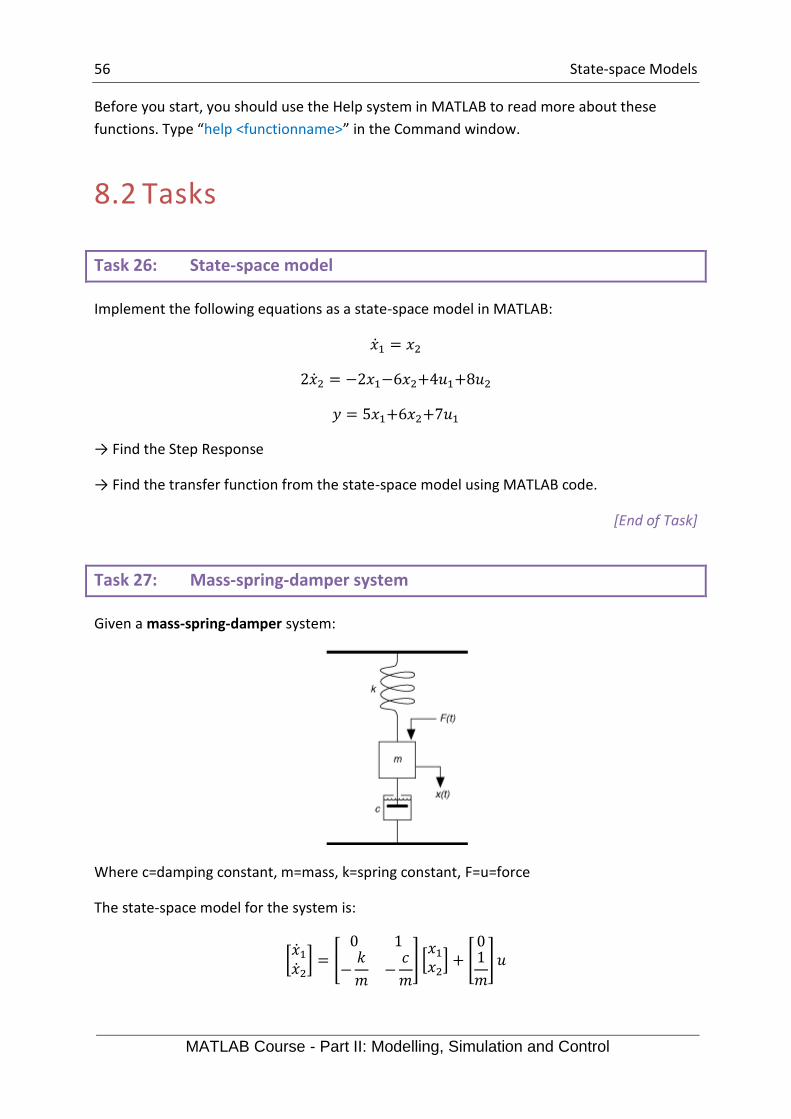
Task 27: Mass-spring-damper system
Given a mass-spring-damper system:
Where c=damping constant, m=mass, k=spring constant, F=u=force
The state-space model for the system is:
[�̇�1�̇�2] = [
0 1
−𝑘
𝑚−𝑐
𝑚
] [𝑥1𝑥2] + [
01
𝑚
]𝑢

57 State-space Models
MATLAB Course - Part II: Modelling, Simulation and Control
𝑦 = [1 0] [𝑥1𝑥2]
Define the state-space model above using the ss function in MATLAB.
Set 𝑐 = 1, 𝑚 = 1, 𝑘 = 50 (try also with other values to see what happens).
→Apply a step in F (u) and use the step function in MATLAB to simulate the result.
→ Find the transfer function from the state-space model
[End of Task]
Task 28: Block Diagram
Find the state-space model from the block diagram below and implement it in MATLAB.
Set
𝑎1 = 5
𝑎2 = 2
And b=1, c=1
→ Simulate the system using the step function in MATLAB
[End of Task]
58 State-space Models
MATLAB Course - Part II: Modelling, Simulation and Control
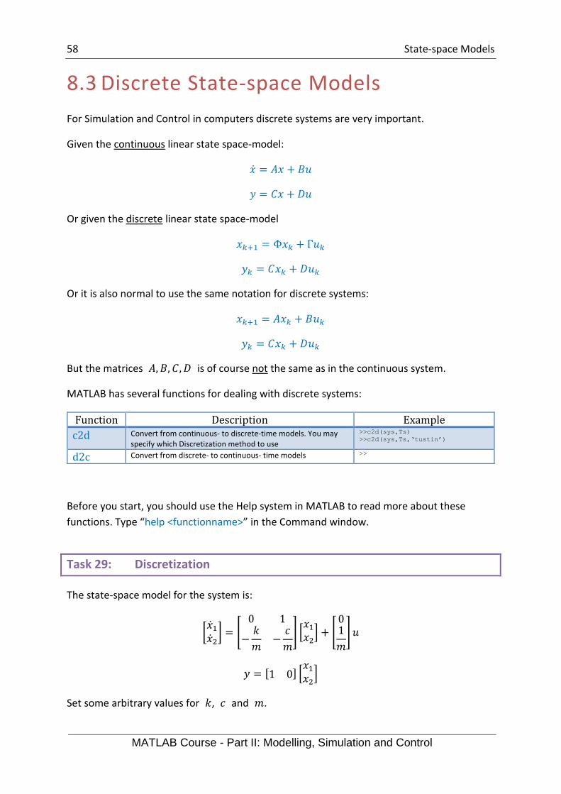
8.3 Discrete State-space Models
For Simulation and Control in computers discrete systems are very important.
Given the continuous linear state space-model:
�̇� = 𝐴𝑥 + 𝐵𝑢
𝑦 = 𝐶𝑥 + 𝐷𝑢
Or given the discrete linear state space-model
𝑥𝑘+1 = Φ𝑥𝑘 + Γ𝑢𝑘
𝑦𝑘 = 𝐶𝑥𝑘 + 𝐷𝑢𝑘
Or it is also normal to use the same notation for discrete systems:
𝑥𝑘+1 = 𝐴𝑥𝑘 + 𝐵𝑢𝑘
𝑦𝑘 = 𝐶𝑥𝑘 + 𝐷𝑢𝑘
But the matrices 𝐴, 𝐵, 𝐶, 𝐷 is of course not the same as in the continuous system.
MATLAB has several functions for dealing with discrete systems:
Function Description Example
c2d Convert from continuous- to discrete-time models. You may specify which Discretization method to use
>>c2d(sys,Ts)
>>c2d(sys,Ts,‘tustin’)
d2c Convert from discrete- to continuous- time models >>
Before you start, you should use the Help system in MATLAB to read more about these
functions. Type “help <functionname>” in the Command window.
Task 29: Discretization
The state-space model for the system is:
[�̇�1�̇�2] = [
0 1
−𝑘
𝑚−𝑐
𝑚
] [𝑥1𝑥2] + [
01
𝑚
]𝑢
𝑦 = [1 0] [𝑥1𝑥2]
Set some arbitrary values for 𝑘, 𝑐 and 𝑚.
59 State-space Models
MATLAB Course - Part II: Modelling, Simulation and Control
Find the discrete State-space model using MATLAB.
[End of Task]
60
9 Frequency Response
In this chapter we assume that you are familiar with basic control theory and frequency
response from previous courses in control theory/process control/cybernetics. If not, you
may skip this chapter.
9.1 Introduction
The frequency response of a system is a frequency dependent function which expresses how
a sinusoidal signal of a given frequency on the system input is transferred through the
system. Each frequency component is a sinusoidal signal having a certain amplitude and a
certain frequency.
The frequency response is an important tool for analysis and design of signal filters and for
analysis and design of control systems. The frequency response can be found experimentally
or from a transfer function model.
We can find the frequency response of a system by exciting the system with a sinusoidal
signal of amplitude A and frequency ω [rad/s] (Note: 𝜔 = 2𝜋𝑓) and observing the response
in the output variable of the system.
The frequency response of a system is defined as the steady-state response of the system to
a sinusoidal input signal. When the system is in steady-state it differs from the input signal
only in amplitude/gain (A) and phase lag (𝜙).
If we have the input signal:
𝑢(𝑡) = 𝑈 𝑠𝑖𝑛𝜔𝑡
The steady-state output signal will be:
𝑦(𝑡) = 𝑈𝐴⏟𝑌
sin (𝜔𝑡 + 𝜙)
Where 𝐴 =𝑌
𝑈 is the ratio between the amplitudes of the output signal and the input signal
(in steady-state).
A and 𝜙 is a function of the frequency ω so we may write 𝐴 = 𝐴(𝜔), 𝜙 = 𝜙(𝜔)
61 Frequency Response
MATLAB Course - Part II: Modelling, Simulation and Control
For a transfer function
𝐻(𝑆) =𝑦(𝑠)
𝑢(𝑠)
We have that:
𝐻(𝑗𝜔) = |𝐻(𝑗𝜔)|𝑒𝑗∠𝐻(𝑗𝜔)
Where 𝐻(𝑗𝜔) is the frequency response of the system, i.e., we may find the frequency
response by setting 𝑠 = 𝑗𝜔 in the transfer function. Bode diagrams are useful in frequency
response analysis. The Bode diagram consists of 2 diagrams, the Bode magnitude diagram,
𝐴(𝜔) and the Bode phase diagram, 𝜙(𝜔).
The Gain function:
𝐴(𝜔) = |𝐻(𝑗𝜔)|
The Phase function:
𝜙(𝜔) = ∠𝐻(𝑗𝜔)
The 𝐴(𝜔)-axis is in decibel (dB), where the decibel value of x is calculated as: 𝒙[𝒅𝑩] =
𝟐𝟎𝒍𝒐𝒈𝟏𝟎𝒙
The 𝜙(𝜔)-axis is in degrees (not radians!)
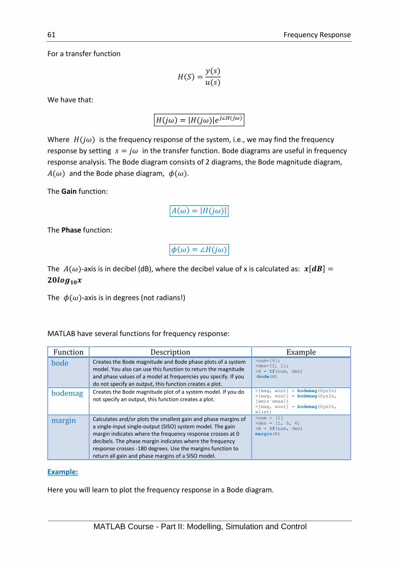
MATLAB have several functions for frequency response:
Function Description Example
bode Creates the Bode magnitude and Bode phase plots of a system model. You also can use this function to return the magnitude and phase values of a model at frequencies you specify. If you do not specify an output, this function creates a plot.
>num=[4];
>den=[2, 1];
>H = tf(num, den)
>bode(H)
bodemag Creates the Bode magnitude plot of a system model. If you do not specify an output, this function creates a plot.
>[mag, wout] = bodemag(SysIn)
>[mag, wout] = bodemag(SysIn,
[wmin wmax])
>[mag, wout] = bodemag(SysIn,
wlist)
margin Calculates and/or plots the smallest gain and phase margins of a single-input single-output (SISO) system model. The gain margin indicates where the frequency response crosses at 0 decibels. The phase margin indicates where the frequency response crosses -180 degrees. Use the margins function to return all gain and phase margins of a SISO model.
>num = [1]
>den = [1, 5, 6]
>H = tf(num, den)
margin(H)
Example:
Here you will learn to plot the frequency response in a Bode diagram.
62 Frequency Response
MATLAB Course - Part II: Modelling, Simulation and Control
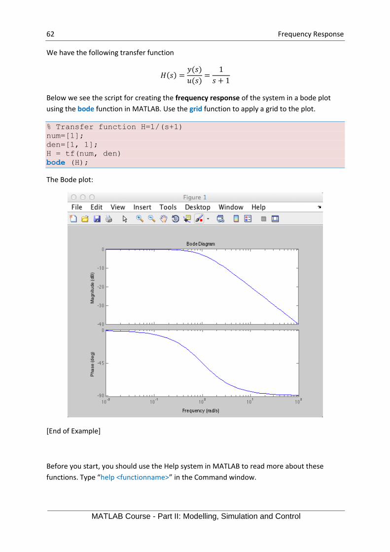
We have the following transfer function
𝐻(𝑠) =𝑦(𝑠)
𝑢(𝑠)=
1
𝑠 + 1
Below we see the script for creating the frequency response of the system in a bode plot
using the bode function in MATLAB. Use the grid function to apply a grid to the plot.
% Transfer function H=1/(s+1)
num=[1];
den=[1, 1];
H = tf(num, den)
bode (H);
The Bode plot:
[End of Example]
Before you start, you should use the Help system in MATLAB to read more about these
functions. Type “help <functionname>” in the Command window.

63 Frequency Response
MATLAB Course - Part II: Modelling, Simulation and Control
9.2 Tasks
Task 30: 1. order system
We have the following transfer function:
𝐻(𝑠) =4
2𝑠 + 1
→ What is the break frequency?
→ Set up the mathematical expressions for 𝐴(𝜔) and 𝜙(𝜔). Use “Pen & Paper” for this
Assignment.
→ Plot the frequency response of the system in a bode plot using the bode function in
MATLAB. Discuss the results.
→ Find 𝐴(𝜔) and 𝜙(𝜔) for the following frequencies using MATLAB code (use the bode
function):
𝝎 𝑨(𝝎)[𝒅𝑩] 𝝓(𝝎)(𝒅𝒆𝒈𝒓𝒆𝒆𝒔)
0.1
0.16
0.25
0.4
0.625
2.5
Make sure 𝐴(𝜔) is in dB.
→ Find 𝐴(𝜔) and 𝜙(𝜔) for the same frequencies above using the mathematical
expressions for 𝐴(𝜔) and 𝜙(𝜔). Tip: Use a For Loop or define a vector w=[0.1, 0.16, 0.25,
0.4, 0.625, 2.5].
[End of Task]
Task 31: Bode Diagram
We have the following transfer function:
𝐻(𝑆) =(5𝑠 + 1)
(2𝑠 + 1)(10𝑠 + 1)
→ What is the break frequencies?

64 Frequency Response
MATLAB Course - Part II: Modelling, Simulation and Control
→ Set up the mathematical expressions for 𝐴(𝜔) and 𝜙(𝜔). Use “Pen & Paper” for this
Assignment.
→ Plot the frequency response of the system in a bode plot using the bode function in
MATLAB. Discuss the results.
→ Find 𝐴(𝜔) and 𝜙(𝜔) for some given frequencies using MATLAB code (use the bode
function).
→ Find 𝐴(𝜔) and 𝜙(𝜔) for the same frequencies above using the mathematical
expressions for 𝐴(𝜔) and 𝜙(𝜔). Tip: use a For Loop or define a vector w=[0.01, 0.1, …].
[End of Task]
9.3 Frequency response Analysis
Here are some important transfer functions to determine the stability of a feedback system.
Below we see a typical feedback system.
9.3.1 Loop Transfer Function
The Loop transfer function 𝑳(𝒔) is defined as follows:
𝐿(𝑠) = 𝐻𝑐𝐻𝑝𝐻𝑚
Where
𝐻𝑐 is the Controller transfer function
𝐻𝑝 is the Process transfer function
𝐻𝑚 is the Measurement (sensor) transfer function
Note! Another notation for 𝐿 is 𝐻0
65 Frequency Response
MATLAB Course - Part II: Modelling, Simulation and Control
9.3.2 Tracking Transfer Function
The Tracking transfer function 𝑻(𝒔) is defined as follows:
𝑇(𝑠) =𝑦(𝑠)
𝑟(𝑠)=
𝐻𝑐𝐻𝑝𝐻𝑚
1 + 𝐻𝑐𝐻𝑝𝐻𝑚=
𝐿(𝑠)
1 + 𝐿(𝑠)= 1 − 𝑆(𝑠)
The Tracking Property is good if the tracking function T has value equal to or close to 1:
|𝑇| ≈ 1
9.3.3 Sensitivity Transfer Function
The Sensitivity transfer function 𝑺(𝒔) is defined as follows:
𝑆(𝑠) =𝑒(𝑠)
𝑟(𝑠)=
1
1 + 𝐿(𝑠)= 1 − 𝑇(𝑠)
The Compensation Property is good if the sensitivity function S has a small value close to
zero:
|𝑆| ≈ 0 𝑜𝑟 |𝑆| ≪ 1
Note!
𝑇(𝑠) + 𝑆(𝑠) =𝐿(𝑠)
1 + 𝐿(𝑠)+
1
1 + 𝐿(𝑠)≡ 1
Frequency Response Analysis of the Tracking Property:
From the equations above we find:
The Tracking Property is good if:
|𝐿(𝑗𝜔)| ≫ 1
The Tracking Property is poor if:
|𝐿(𝑗𝜔)| ≪ 1
If we plot L, T and S in a Bode plot we get a plot like this:

66 Frequency Response
MATLAB Course - Part II: Modelling, Simulation and Control
Where the following Bandwidths 𝜔𝑡, 𝜔𝑐, 𝜔𝑠 are defined:
𝝎𝒄 – crossover-frequency – the frequency where the gain of the Loop transfer function
𝐿(𝑗𝜔) has the value:
1 = 0𝑑𝐵
𝝎𝒕 – the frequency where the gain of the Tracking function 𝑇(𝑗𝜔) has the value:
1
√2≈ 0.71 = −3𝑑𝐵
𝝎𝒔 - the frequency where the gain of the Sensitivity transfer function 𝑆(𝑗𝜔) has the value:
1 −1
√2≈ 0.29 = −11𝑑𝐵
Task 32: Frequency Response Analysis
Given the following system:
Process transfer function:
𝐻𝑝 =𝐾
𝑠
67 Frequency Response
MATLAB Course - Part II: Modelling, Simulation and Control
Where 𝐾 =𝐾𝑠
𝜚𝐴, where 𝐾𝑠 = 0,556, 𝐴 = 13,4, 𝜚 = 145
Measurement (sensor) transfer function:
𝐻𝑚 = 𝐾𝑚
Where 𝐾𝑚 = 1.
Controller transfer function (PI Controller):
𝐻𝑐 = 𝐾𝑝 +𝐾𝑝
𝑇𝑖𝑠
Set Kp = 1,5 og Ti = 1000 sec.
→ Define the Loop transfer function 𝑳(𝒔), Sensitivity transfer function 𝑺(𝒔) and Tracking
transfer function 𝑻(𝒔) and in MATLAB.
→ Plot the Loop transfer function 𝐿(𝑠), the Tracking transfer function 𝑇(𝑠) and the
Sensitivity transfer function 𝑆(𝑠) in the same Bode diagram. Use, e.g., the bodemag
function in MATLAB.
→ Find the bandwidths 𝜔𝑡, 𝜔𝑐, 𝜔𝑠 from the plot above.
→ Plot the step response for the Tracking transfer function 𝑇(𝑠)
[End of Task]
9.4 Stability Analysis of Feedback Systems
Gain Margin (GM) and Phase Margin (PM) are important design criteria for analysis of
feedback control systems.
A dynamic system has one of the following stability properties:
• Asymptotically stable system
• Marginally stable system
• Unstable system

68 Frequency Response
MATLAB Course - Part II: Modelling, Simulation and Control
The Gain Margin – GM (Δ𝐾) is how much the loop gain can increase before the system
become unstable.
The Phase Margin - PM (𝜑) is how much the phase lag function of the loop can be reduced
before the loop becomes unstable.
Where:
• 𝝎𝟏𝟖𝟎 (gain margin frequency - gmf) is the gain margin frequency/frequencies, in
radians/second. A gain margin frequency indicates where the model phase crosses -
180 degrees.
• GM (Δ𝐾) is the gain margin(s) of the system.
• 𝝎𝒄 (phase margin frequency - pmf) returns the phase margin frequency/frequencies,
in radians/second. A phase margin frequency indicates where the model magnitude
crosses 0 decibels.
• PM (𝜑) is the phase margin(s) of the system.
Note! 𝝎𝟏𝟖𝟎 and 𝝎𝒄 are called the crossover-frequencies
The definitions are as follows:
Gain Crossover-frequency - 𝝎𝒄 :
|𝐿(𝑗𝜔𝑐)| = 1 = 0𝑑𝐵
Phase Crossover-frequency - 𝝎𝟏𝟖𝟎 :
∠𝐿(𝑗𝜔180) = −180𝑜
Gain Margin - GM (𝚫𝑲):
69 Frequency Response
MATLAB Course - Part II: Modelling, Simulation and Control
𝐺𝑀 =1
|𝐿(𝑗𝜔180)|
or:
𝐺𝑀 [𝑑𝐵] = −|𝐿(𝑗𝜔180)| [𝑑𝐵]
Phase margin PM (𝝋):
𝑃𝑀 = 180𝑜 + ∠𝐿(𝑗𝜔𝑐)
We have that:
• Asymptotically stable system: 𝝎𝒄 < 𝝎𝟏𝟖𝟎
• Marginally stable system: 𝝎𝒄 = 𝝎𝟏𝟖𝟎
• Unstable system: 𝝎𝒄 > 𝝎𝟏𝟖𝟎
We use the following functions in MATLAB: tf, bode, margins and margin.
Task 33: Stability Analysis
Given the following system:
𝐻(𝑆) =1
𝑠(𝑠 + 1)2
We will find the crossover-frequencies for the system using MATLAB. We will also find also
the gain margins and phase margins for the system.
Plot a bode diagram where the crossover-frequencies, GM and PM are illustrated. Tip! Use
the margin function in MATLAB.
[End of Task]

70
10 Additional Tasks
If you have time left or need more practice, solve the tasks below. Its highly recommended
to solve these tasks as well, since some of these will most likely be part of the final test.
Task 34: ODE Solvers
Use the ode45 function to solve and plot the results of the following differential equation in
the interval [𝑡0, 𝑡𝑓]:
𝟑𝒘′ +𝟏
𝟏 + 𝒕𝟐𝒘 = 𝒄𝒐𝒔𝒕, 𝑡0 = 0, 𝑡𝑓 = 5,𝑤(𝑡0) = 1
[End of Task]
Task 35: Mass-spring-damper system
Given a mass-spring-damper system:
Where c=damping constant, m=mass, k=spring constant, F=u=force
The state-space model for the system is:
[�̇�1�̇�2] = [
0 1
−𝑘
𝑚−𝑐
𝑚
] [𝑥1𝑥2] + [
01
𝑚
]𝑢
Set 𝑐 = 1,𝑚 = 1, 𝑘 = 50.
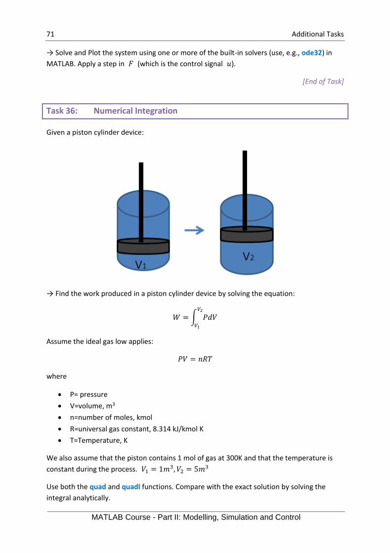
71 Additional Tasks
MATLAB Course - Part II: Modelling, Simulation and Control
→ Solve and Plot the system using one or more of the built-in solvers (use, e.g., ode32) in
MATLAB. Apply a step in 𝐹 (which is the control signal 𝑢).
[End of Task]
Task 36: Numerical Integration
Given a piston cylinder device:
→ Find the work produced in a piston cylinder device by solving the equation:
𝑊 = ∫ 𝑃𝑑𝑉𝑉2
𝑉1
Assume the ideal gas low applies:
𝑃𝑉 = 𝑛𝑅𝑇
where
• P= pressure
• V=volume, m3
• n=number of moles, kmol
• R=universal gas constant, 8.314 kJ/kmol K
• T=Temperature, K
We also assume that the piston contains 1 mol of gas at 300K and that the temperature is
constant during the process. 𝑉1 = 1𝑚3, 𝑉2 = 5𝑚
3
Use both the quad and quadl functions. Compare with the exact solution by solving the
integral analytically.

72 Additional Tasks
MATLAB Course - Part II: Modelling, Simulation and Control
[End of Task]
Task 37: State-space model
The following model of a pendulum is given:
�̇�1 = 𝑥2
�̇�2 = −𝑔
𝑟𝑥1 −
𝑏
𝑚𝑟2𝑥2
where m is the mass, r is the length of the arm of the pendulum, g is the gravity, b is a
friction coefficient.
→ Define the state-space model in MATLAB
→ Solve the differential equations in MATLAB and plot the results.
Use the following values 𝑔 = 9.81,𝑚 = 8, 𝑟 = 5, 𝑏 = 10
[End of Task]
Task 38: lsim
Given a mass-spring-damper system:
Where c=damping constant, m=mass, k=spring constant, F=u=force
The state-space model for the system is:
[�̇�1�̇�2] = [
0 1
−𝑘
𝑚−𝑐
𝑚
] [𝑥1𝑥2] + [
01
𝑚
]𝑢
𝑦 = [1 0] [𝑥1𝑥2]

73 Additional Tasks
MATLAB Course - Part II: Modelling, Simulation and Control
→ Simulate the system using the lsim function in the Control System Toolbox.
Set c=1, m=1, k=50.
[End of Task]

74
Appendix A – MATLAB
Functions
Numerical Techniques
Here are some descriptions for the most used MATLAB functions for Numerical Techniques.
Solving Ordinary Differential Equations
MATLAB offers lots of ode solvers, e.g.:
Function Description Example
ode23
ode45
Interpolation
MATLAB offers functions for interpolation, e.g.:
Function Description Example
interp1
Curve Fitting
Here are some of the functions available in MATLAB used for curve fitting:
Function Description Example
polyfit P = POLYFIT(X,Y,N) finds the coefficients of a polynomial P(X) of degree N that fits the data Y best in a least-squares sense. P is a row vector of length N+1 containing the polynomial coefficients in descending powers, P(1)*X^N + P(2)*X^(N-1) +...+ P(N)*X + P(N+1).
>>polyfit(x,y,1)
polyval Evaluate polynomial. Y = POLYVAL(P,X) returns the value of a polynomial P evaluated at X. P is a vector of length N+1 whose elements are the coefficients of the polynomial in descending powers. Y = P(1)*X^N + P(2)*X^(N-1) + ... + P(N)*X + P(N+1)

75 Appendix A – MATLAB Functions
MATLAB Course - Part II: Modelling, Simulation and Control
Numerical Differentiation
MATLAB offers functions for numerical differentiation, e.g.:
Function Description Example
diff Difference and approximate derivative. DIFF(X), for a vector X, is [X(2)-X(1) X(3)-X(2) ... X(n)-X(n-1)].
>> dydx_num=diff(y)./diff(x);
polyder Differentiate polynomial. POLYDER(P) returns the derivative of the polynomial whose coefficients are the elements of vector P. POLYDER(A,B) returns the derivative of polynomial A*B.
>>p=[1,2,3];
>>polyder(p)
Numerical Integration
MATLAB offers functions for numerical integration, such as:
Function Description Example
diff Difference and approximate derivative. DIFF(X), for a vector X, is [X(2)-X(1) X(3)-X(2) ... X(n)-X(n-1)].
>> dydx_num=diff(y)./diff(x);
quad Numerically evaluate integral, adaptive Simpson quadrature. Q = QUAD(FUN,A,B) tries to approximate the integral of calar-valued function FUN from A to B. FUN is a function handle. The function Y=FUN(X) should accept a vector argument X and return a vector result Y, the integrand evaluated at each element of X. Uses adaptive Simpson quadrature method
>>
quadl Same as quad, but uses adaptive Lobatto quadrature method >>
polyint Integrate polynomial analytically. POLYINT(P,K) returns a polynomial representing the integral of polynomial P, using a scalar constant of integration K.
Optimization
MATLAB offers functions for local minimum, such as:
Function Description Example
fminbnd X = FMINBND(FUN,x1,x2) attempts to find a local minimizer X of the function FUN in the interval x1 < X < x2. FUN is a function handle. FUN accepts scalar input X and returns a scalar function value F evaluated at X. FUN can be specified using @. FMINBND is a single-variable bounded nonlinear function minimization.
>> x = fminbnd(@cos,3,4)
x =
3.1416
fminsearch X = FMINSEARCH(FUN,X0) starts at X0 and attempts to find a local minimizer X of the function FUN. FUN is a function handle. FUN accepts input X and returns a scalar function value F evaluated at X. X0 can be a scalar, vector or matrix. FUN can be specified using @. FMINSEARCH is a multidimensional unconstrained nonlinear function minimization.
>> x = fminsearch(@sin,3)
x =
4.7124

76 Appendix A – MATLAB Functions
MATLAB Course - Part II: Modelling, Simulation and Control
Control and Simulation
Here are some descriptions for the most used MATLAB functions for Control and Simulation.
Function Description Example
plot Generates a plot. plot(y) plots the columns of y against the indexes of the columns.
>X = [0:0.01:1];
>Y = X.*X;
>plot(X, Y)
tf Creates system model in transfer function form. You also can use this function to state-space models to transfer function form.
>num=[1];
>den=[1, 1, 1];
>H = tf(num, den)
pole Returns the locations of the closed-loop poles of a system model.
>num=[1]
>den=[1,1]
>H=tf(num,den)
>poles(H)
step Creates a step response plot of the system model. You also can use this function to return the step response of the model outputs. If the model is in state-space form, you also can use this function to return the step response of the model states. This function assumes the initial model states are zero. If you do not specify an output, this function creates a plot.
>num=[1,1];
>den=[1,-1,3];
>H=tf(num,den);
>t=[0:0.01:10];
>step(H,t);
lsim Creates the linear simulation plot of a system model. This function calculates the output of a system model when a set of inputs excite the model, using discrete simulation. If you do not specify an output, this function creates a plot.
>t = [0:0.1:10]
>u = sin(0.1*pi*t)'
>lsim(SysIn, u, t)
conv Computes the convolution of two vectors or matrices. >C1 = [1, 2, 3];
>C2 = [3, 4];
>C = conv(C1, C2)
series Connects two system models in series to produce a model SysSer with input and output connections you specify
>Hseries = series(H1,H2)
feedback Connects two system models together to produce a closed-loop model using negative or positive feedback connections
>SysClosed = feedback(SysIn_1,
SysIn_2)
ss Constructs a model in state-space form. You also can use this function to convert transfer function models to state-space form.
>A = eye(2)
>B = [0; 1]
>C = B'
>SysOutSS = ss(A, B, C)
bode Creates the Bode magnitude and Bode phase plots of a system model. You also can use this function to return the magnitude and phase values of a model at frequencies you specify. If you do not specify an output, this function creates a plot.
>num=[4];
>den=[2, 1];
>H = tf(num, den)
>bode(H)
bodemag Creates the Bode magnitude plot of a system model. If you do not specify an output, this function creates a plot.
>[mag, wout] = bodemag(SysIn)
>[mag, wout] = bodemag(SysIn,
[wmin wmax])
>[mag, wout] = bodemag(SysIn,
wlist)
margin Calculates and/or plots the smallest gain and phase margins of a single-input single-output (SISO) system model. The gain margin indicates where the frequency response crosses at 0 decibels. The phase margin indicates where the frequency response crosses -180 degrees. Use the margins function to return all gain and phase margins of a SISO model.
>num = [1]
>den = [1, 5, 6]
>H = tf(num, den)
margin(H)
margins Calculates all gain and phase margins of a single-input single-output (SISO) system model. The gain margins indicate where the frequency response crosses at 0 decibels. The phase margins indicate where the frequency response crosses -180 degrees. Use the margin function to return only the smallest gain and phase margins of a SISO model.
>[gmf, gm, pmf, pm] = margins(H)
c2d Convert from continuous- to discrete-time models
d2c Convert from discrete- to continuous-time models

Hans-Petter Halvorsen
E-mail: [email protected]
Blog: http://www.halvorsen.blog
University of South-Eastern Norway
www.usn.no