11

Lecture Series – 5

Plotting in MATLAB

Lecture Series by

Shameer Koya

PLOTTING

plot (x, y, ‘color style marker’)

xlabel (‘text’)

ylabel (‘text’)

title (‘text’)

grid on / off

axis

subplot (m, n, p)

legend (‘text1’, ‘text2’, ‘text3’)

Other commands - semilogx, semilogy, axis, colordef,

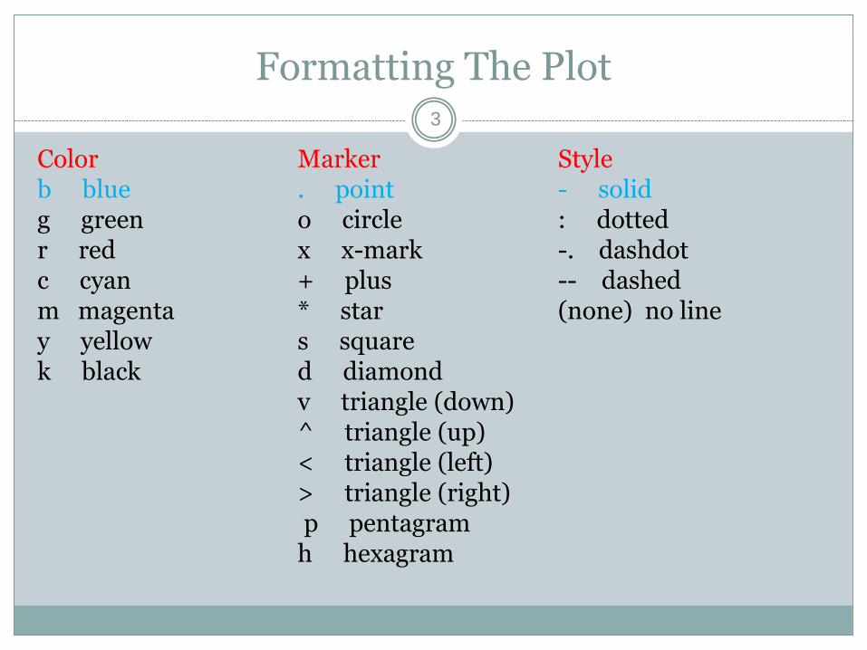
Formatting The Plot

Color Marker Styleb blue . point - solidg green o circle : dottedr red x x-mark -. dashdotc cyan + plus -- dashed m magenta * star (none) no liney yellow s squarek black d diamond

v triangle (down)^ triangle (up)< triangle (left)> triangle (right)p pentagram

h hexagram

3

4

Plot

PLOT Linear plot.

PLOT(X,Y) plots vector Y versus vector X

PLOT(Y) plots the columns of Y versus their index

PLOT(X,Y,S) with plot symbols and colors

x = [-3 -2 -1 0 1 2 3];

y1 = (x.^2) -1;

plot(x, y1,'bo-.');

Example

5

Plot Properties

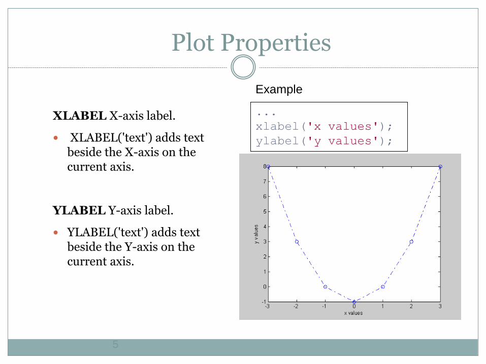
XLABEL X-axis label.

XLABEL('text') adds text beside the X-axis on the current axis.

YLABEL Y-axis label.

YLABEL('text') adds text beside the Y-axis on the current axis.

...

xlabel('x values');

ylabel('y values');

Example

6

Hold

HOLD Hold current graph.

HOLD ON holds the current plot and all axis properties so that subsequent graphing commands add to the existing graph.

HOLD OFF returns to the default mode

HOLD, by itself, toggles the hold state.

...

hold on;

y2 = x + 2;

plot(x, y2, 'g+:');

Example

7

Subplot

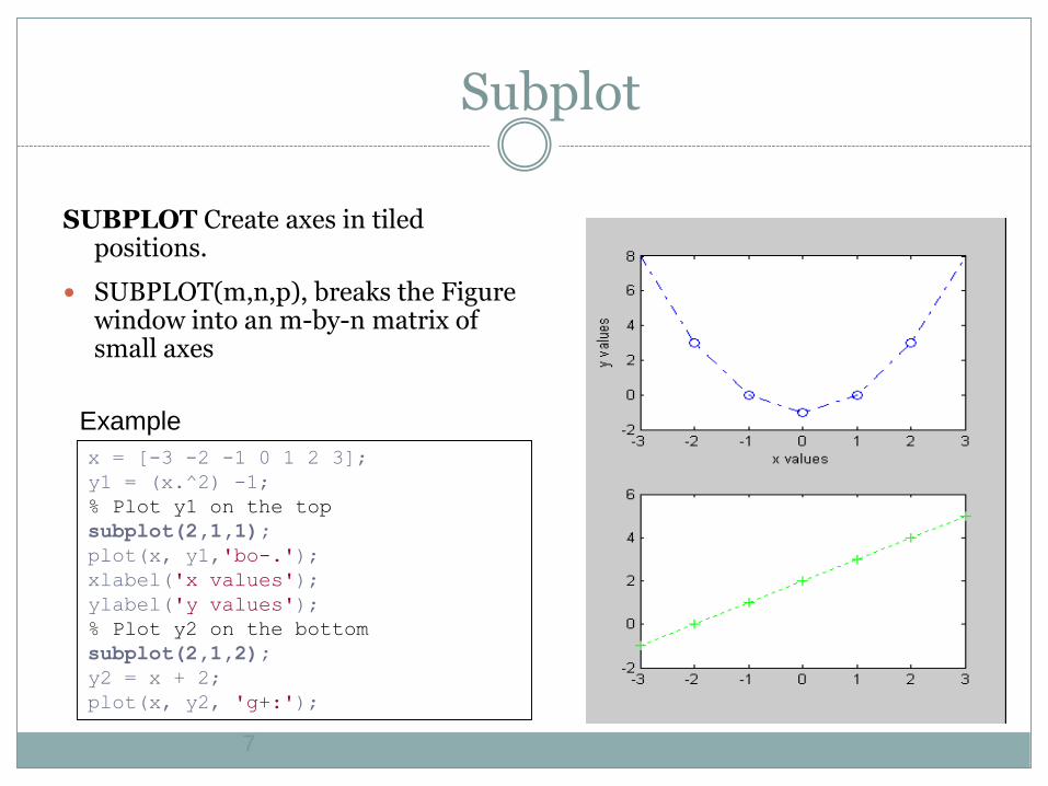
SUBPLOT Create axes in tiled positions.

SUBPLOT(m,n,p), breaks the Figure window into an m-by-n matrix of small axes

x = [-3 -2 -1 0 1 2 3];

y1 = (x.^2) -1;

% Plot y1 on the top

subplot(2,1,1);

plot(x, y1,'bo-.');

xlabel('x values');

ylabel('y values');

% Plot y2 on the bottom

subplot(2,1,2);

y2 = x + 2;

plot(x, y2, 'g+:');

Example

AXIS Control

axis scaling and appearance.

axis([xmin xmax ymin ymax])

Sets scaling for the x- and y-axes on the current plot.

axis auto - returns the axis scaling to its default, automatic mode

axis off - turns off all axis labeling, tick marks and background.

axis on - turns axis labeling, tick marks and background back on.

axis equal – makes both axes equal length

8

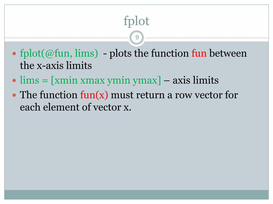
fplot

fplot(@fun, lims) - plots the function fun between the x-axis limits

lims = [xmin xmax ymin ymax] – axis limits

The function fun(x) must return a row vector for each element of vector x.

9

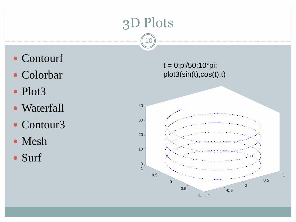
3D Plots

Contourf

Colorbar

Plot3

Waterfall

Contour3

Mesh

Surf

10

t = 0:pi/50:10*pi;

plot3(sin(t),cos(t),t)

-1

-0.5

0

0.5

1

-1

-0.5

0

0.5

10

10

20

30

40

11

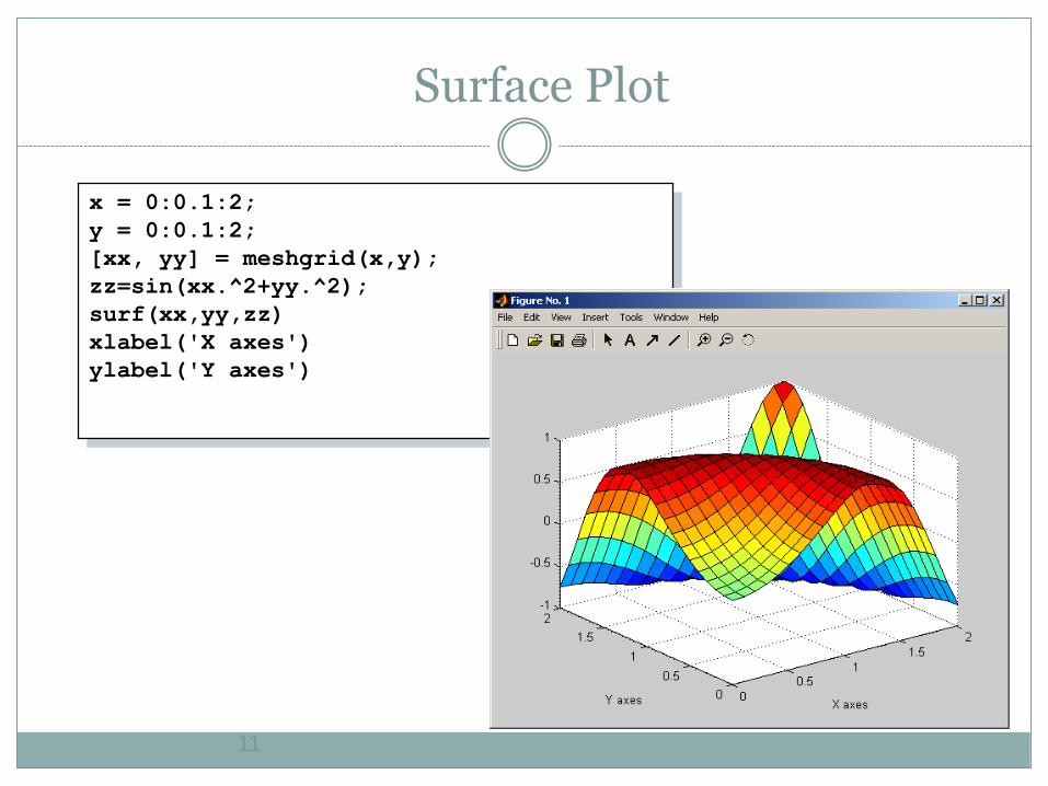
Surface Plot

x = 0:0.1:2;

y = 0:0.1:2;

[xx, yy] = meshgrid(x,y);

zz=sin(xx.^2+yy.^2);

surf(xx,yy,zz)

xlabel('X axes')

ylabel('Y axes')

12

contourf-colorbar-plot3-waterfall-contour3-mesh-surf

3 D Surface Plot

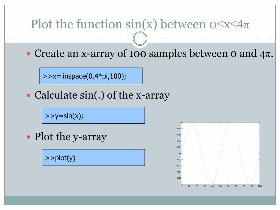
Plot the function sin(x) between 0≤x≤4π

Create an x-array of 100 samples between 0 and 4π.

Calculate sin(.) of the x-array

Plot the y-array

>>x=linspace(0,4*pi,100);

>>y=sin(x);

>>plot(y)

0 10 20 30 40 50 60 70 80 90 100-1

-0.8

-0.6

-0.4

-0.2

0

0.2

0.4

0.6

0.8

1

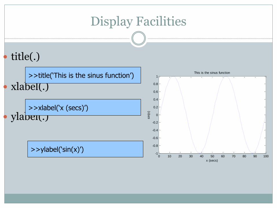
Display Facilities

title(.)

xlabel(.)

ylabel(.)

>>title(‘This is the sinus function’)

>>xlabel(‘x (secs)’)

>>ylabel(‘sin(x)’)0 10 20 30 40 50 60 70 80 90 100

-1

-0.8

-0.6

-0.4

-0.2

0

0.2

0.4

0.6

0.8

1This is the sinus function

x (secs)

sin

(x)

15

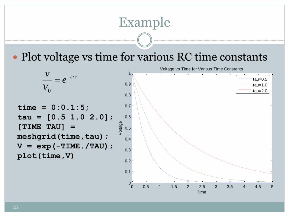
Example

Plot voltage vs time for various RC time constants

/

0

teV

v

0 0.5 1 1.5 2 2.5 3 3.5 4 4.5 50

0.1

0.2

0.3

0.4

0.5

0.6

0.7

0.8

0.9

1Voltage vs Time for Various Time Constants

Time

Voltage

tau=0.5

tau=1.0

tau=2.0

time = 0:0.1:5;

tau = [0.5 1.0 2.0];

[TIME TAU] =

meshgrid(time,tau);

V = exp(-TIME./TAU);

plot(time,V)

16

Thanks

Questions ??

Plot a sphere, which is defined as

[x(t, s), y(t, s), z(t, s)] = [cos(t) cos(s), cos(t) sin(s), sin(t)]

for t, s = [0, 2 ] (use ‘surf’).

Make first equal axes, then remove them. Use ‘shading interp’ to remove

black lines

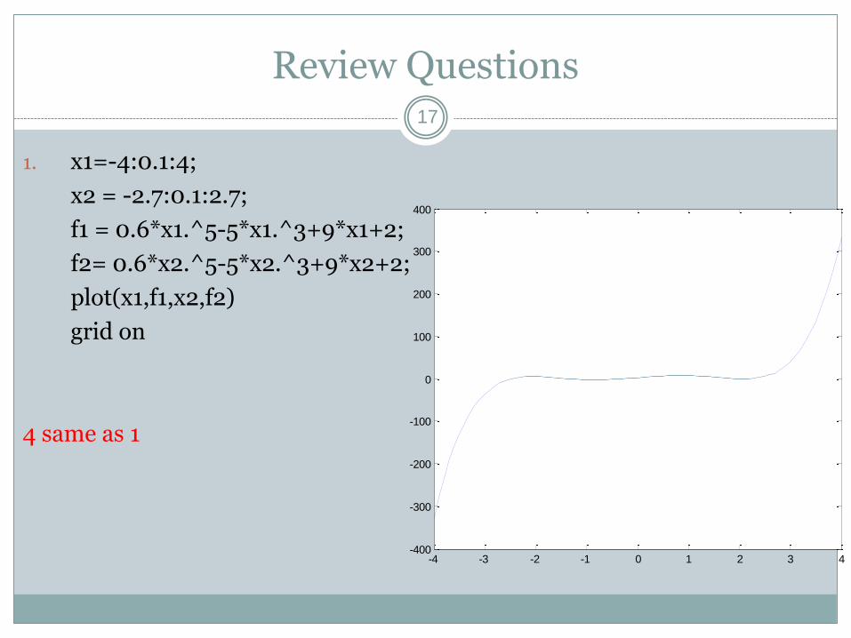
Review Questions

1. x1=-4:0.1:4;

x2 = -2.7:0.1:2.7;

f1 = 0.6*x1.^5-5*x1.^3+9*x1+2;

f2= 0.6*x2.^5-5*x2.^3+9*x2+2;

plot(x1,f1,x2,f2)

grid on

4 same as 1

17

-4 -3 -2 -1 0 1 2 3 4-400

-300

-200

-100

0

100

200

300

400

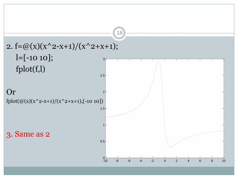
2. f=@(x)(x^2-x+1)/(x^2+x+1);

l=[-10 10];

fplot(f,l)

Orfplot(@(x)(x^2-x+1)/(x^2+x+1),[-10 10])

3. Same as 2

18

-10 -8 -6 -4 -2 0 2 4 6 8 100

0.5

1

1.5

2

2.5

3

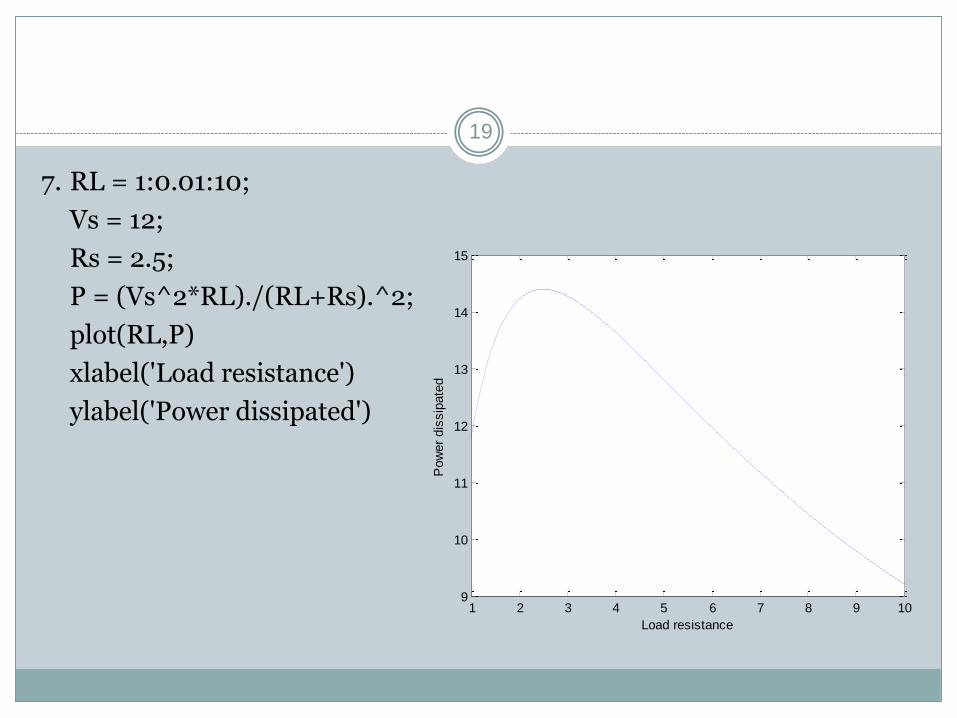
7. RL = 1:0.01:10;

Vs = 12;

Rs = 2.5;

P = (Vs^2*RL)./(RL+Rs).^2;

plot(RL,P)

xlabel('Load resistance')

ylabel('Power dissipated')

19

1 2 3 4 5 6 7 8 9 109

10

11

12

13

14

15

Load resistance

Pow

er

dis

sip

ate

d