Matlab Training Sessions 6,7:Plotting

Course Outline

Weeks:

1. Introduction to Matlab and its Interface (Jan 13 2009)

2. Fundamentals (Operators)

3. Fundamentals (Flow)

4. Importing Data

5. Functions and M-Files

6. Plotting (2D and 3D)

7. Statistical Tools in Matlab

8. Analysis and Data Structures

Course Website:

http://www.queensu.ca/neurosci/matlab.php

Week 5 Lecture Outline

Plotting Data

A. Basics

B. Generating data

C. 2D Plots (Line, Scatter, Bar)

D. Plot Features

Basics• Matlab has a powerful plotting engine that can

generate a wide variety of plots.

Generating Data• Matlab does not understand functions, it can

only use arrays of numbers.– a=t2

– b=sin(2*pi*t)– c=e-10*t note: matlab command is exp()– d=cos(4*pi*t)– e=2t3-4t2+t

• Generate it numerically over specific range• Try and generate a-e over the interval 0:0.01:2

t=0:0.01:10; %make x vector

y=t.^2; %now we have the appropriate y

% but only over the specified range

Line/Scatter

• Simplest plot function is plot()• Try typing plot(y)

– Matlab automatically generates a figure and draws the data and connects its lines

– Looks right, but the x axis units are incorrect

• Type plot(x,y), will look identical but have correct x-axis units

• Plot(x1,y1,s1,x2,y2,s2, …) many plots in one command• Plot(x) where x is a matrix, will result in plotting each

column as a separate trace

Line/Scatter

• Plot a and then plot b– What do you see?– Only b

• Matlab will replace the current plot with any new one unless you specifically tell it not to

• To have both plots on one figure use the hold on command

• To make multiple plots use the figure command

plot(t,a)

plot(t,b)

% Put a and b on one plot

plot(t,a);

hold on;

plot(t,b);

% Make two plots

plot(t,a);

figure;

plot(t,b);

Hold On / Hold Off

• Hold on command only needs to be issued once per figure, thus calling hold on will result in all subsequent plot commands going to one figure unless a new figure command is issued or hold off is used.

plot(a);Hold on;plot(b);plot(c);Hold off;Figure;plot(d);

plot(a);Hold on;plot(b);plot(c);Hold off;plot(d);

plot(a);Hold on;plot(b);plot(c);Figure;plot(d);

Linespec• Currently, all the plots were done in the Matlab

default color … blue• This and many other features can be changed

by selecting a different option within the plot command

% red linePlot(t,a,’r’);Hold on;% black linePlot(t,b,’k’);% green dotsPlot(t,c,’g.’);% cyan x’sPlot(t,d,’cx’)% dashed magenta % line with o’sPlot(t,e,’--om’)

Linespec• Now we have added color, line style and markers to the data• We can also modify line width, marker edge and fill color and marker

size

% dashed magenta % line with o’s, …Plot(t,e,’--om’, ‘LineWidth’,3,'MarkerEdgeColor',‘k‘, 'MarkerFaceColor',‘y‘, MarkerSize,9)

Labels, Title and Legend• To add labels to the x and y axes, we can use the xlabel and ylabel

commands• To add a title, use the title command• To add a legend, use the legend command

plot(t,a,t,b,’r’,t,c,’--om’); %generate all plots in one shottitle(‘Random Plots’)xlabel(‘time(ms)’);ylabel(‘f(t)’)legend(‘Function 1’,’Function 2’,’Function 3’);

Quick Assignment 1• Plot a as a thick black line• Plot b as a series of red circles. • Label each axis, add a title and a legend

0 0.2 0.4 0.6 0.8 1 1.2 1.4 1.6 1.8 2-1

-0.5

0

0.5

1

1.5

2

2.5

3

3.5

4

Time (ms)

f(t)

Mini Assignment #1

t2

sin(2*pi*t)

Quick Assignment 1

0 0.2 0.4 0.6 0.8 1 1.2 1.4 1.6 1.8 2-1

-0.5

0

0.5

1

1.5

2

2.5

3

3.5

4

Time (ms)

f(t)

Mini Assignment #1

t2

sin(2*pi*t)

figureplot(t,a,'k','LineWidth',3); hold on;plot(t,b,'ro')xlabel('Time (ms)');ylabel('f(t)');legend('t^2','sin(2*pi*t)');title('Mini Assignment #1')

Axis commands• We can alter the displayed range and other parameters of the plot by

using the axis command– Axis([xmin xmax ymin ymax])– Axis equal;– Axis square;

Figure;Plot(t,a,’r’);Axis([-2 2 -2 2]);

-2 -1.5 -1 -0.5 0 0.5 1 1.5 2-2

-1.5

-1

-0.5

0

0.5

1

1.5

2

Error Bars• In addition to markers, matlab can generate error bars for each

datapoint using the errorbar command– errorbar(x,y,e) or errorbar(x,y,ll,lu);– Will generate line plus error bars at y+/-e or (y-ll,y+lu)

t2 = 0:1:10;f = t2+(rand(1,length(t2))-0.5);err1 = 0.1*f;err2_l = 0.1*f;err2_u = 0.25*f;errorbar(t2,f,err1);figure;errorbar(t2,f,err2_l, err2_u);

-2 0 2 4 6 8 10 120

2

4

6

8

10

12

-2 0 2 4 6 8 10 120

2

4

6

8

10

12

14

Subplots• So far we have only been generating individual plots• Matlab can also generate a matrix of plots using the subplot command

figure;subplot(2,2,1)plot(t,a);subplot(2,2,2)plot(t,b);subplot(2,2,3)plot(t,c);subplot(2,2,4)plot(t,d);

0 0.5 1 1.5 20

0.5

1

1.5

2

2.5

3

3.5

4

0 0.5 1 1.5 2-1

-0.5

0

0.5

1

0 0.5 1 1.5 20

0.2

0.4

0.6

0.8

1

0 0.5 1 1.5 2-1

-0.5

0

0.5

1

Quick Assignment 2• Generate a 3x1 array

of figures, each with a title

• Axis range of plots 1 and 2 should be 0 to 1 on x and y

• Plot 1 should include function a and b (color code)

• Plot 2 should include c and d (color code)

• Plot 3 should include f with error bars of your liking

0 0.1 0.2 0.3 0.4 0.5 0.6 0.7 0.8 0.9 10

0.5

1Functions a and b

0 0.1 0.2 0.3 0.4 0.5 0.6 0.7 0.8 0.9 10

0.5

1Functions c and d

-2 0 2 4 6 8 10 120

10

20function f with errorbars

Quick Assignment 2

0 0.1 0.2 0.3 0.4 0.5 0.6 0.7 0.8 0.9 10

0.5

1Functions a and b

0 0.1 0.2 0.3 0.4 0.5 0.6 0.7 0.8 0.9 10

0.5

1Functions c and d

-2 0 2 4 6 8 10 120

10

20function f with errorbars

figuresubplot(3,1,1)plot(t,a,t,b,'r');axis([0 1 0 1]);title('Functions a and b')subplot(3,1,2)plot(t,c,t,d,'m');axis([0 1 0 1]);title('Functions c and d')subplot(3,1,3)errorbar(t2,f,err1);title('function f with errorbars')

Bar Graphs• So far we have focused on line/scatter plots, the other most common

plot type is a bar graph• Matlab bar(x,y,width) command will generate a bar graph that is

related to the underlying functions where the width of each bar is specified by width (default = 1);

• Can be used with subplot and all the other features we have discussed so far

t3 = 0:1:25;f = sqrt(t3);bar(t3,f);

-5 0 5 10 15 20 25 300

0.5

1

1.5

2

2.5

3

3.5

4

4.5

5

Histograms• Matlab hist(y,m) command will generate a frequency histogram of

vector y distributed among m bins• Also can use hist(y,x) where x is a vector defining the bin centers

– Note you can use histc function if you want to define bin edges instead

• Can be used with subplot and all the other features we have discussed so far

hist(b,10);Figure;Hist(b,[-1 -0.75 0 0.25 0.5 0.75 1]);

-1.5 -1 -0.5 0 0.5 1 1.50

5

10

15

20

25

30

35

40

-1 -0.8 -0.6 -0.4 -0.2 0 0.2 0.4 0.6 0.8 10

5

10

15

20

25

30

35

40

45

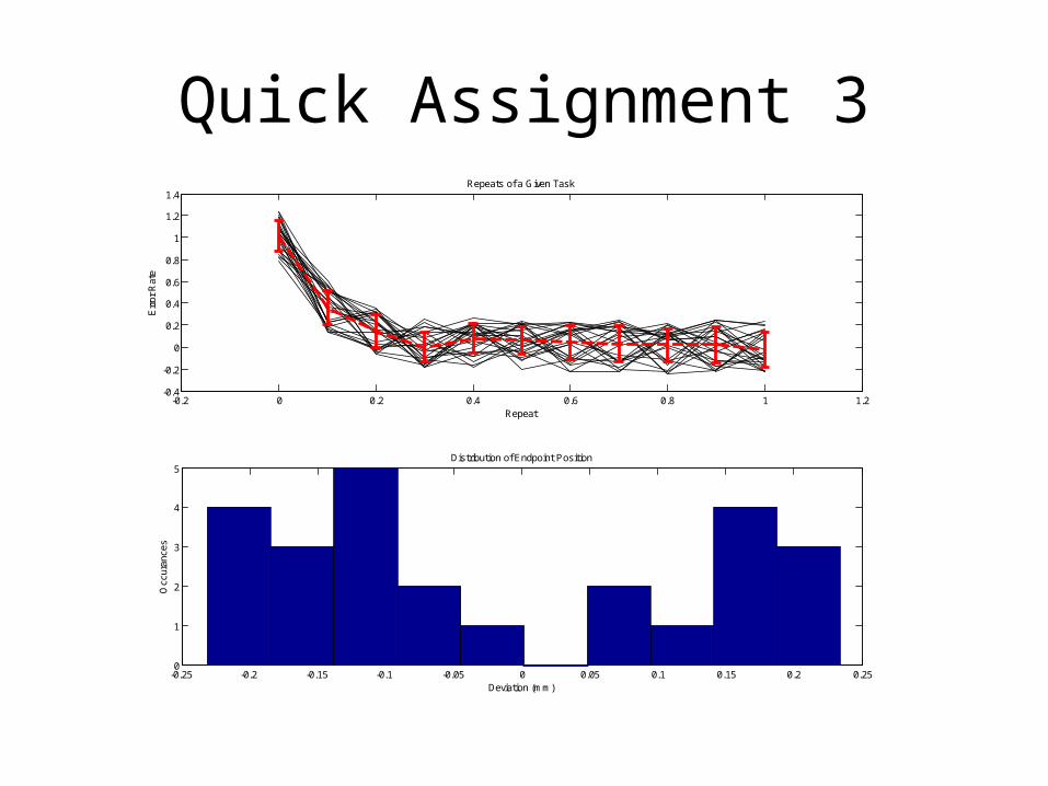
Quick Assignment 3

• Generate the following data set– It results in multiple noisy repeats of some trial

• Create mean_x to be the mean of all the trials at each point of x

• Create std_x to be the standard deviation of all trials at each point of x

• Add labels and titles

t = 0:0.1:1for(i=1:25)

x(i,:) = exp(-10.*t) + 0.5*(rand(1,length(t))-0.5);end

Quick Assignment 3

• Make a plot that is to include 2 subplots• Plot #1:

– Plot each individual trial (25 lines) in thin dotted black lines, • tip: remember about how matlab interprets matricies for the plot

command.

– Plot the mean of the trials with a thick, red, dashed line and error lines surrounding each datapoint that correspond to the standard deviation of each of the points

• Plot #2:– A histogram that expresses the distribution of the signal at the

end of each trial (last sample)

Quick Assignment 3

-0.2 0 0.2 0.4 0.6 0.8 1 1.2-0.4

-0.2

0

0.2

0.4

0.6

0.8

1

1.2

1.4Repeats of a Given Task

Repeat

Err

or R

ate

-0.25 -0.2 -0.15 -0.1 -0.05 0 0.05 0.1 0.15 0.2 0.250

1

2

3

4

5Distribution of Endpoint Position

Deviation (mm)

Occ

uran

ces

t = 0:0.1:1for(i=1:25) x(i,:) = exp(-10.*t) + 0.5*(rand(1,length(t))-0.5);endmean_x = mean(x);std_x = std(x);figuresubplot(2,1,1)plot(t,x,'k'); hold on;errorbar(t,mean_x,std_x,'--r','LineWidth', 3);title('Repeats of a Given Task')xlabel('Repeat');ylabel('Error Rate'); subplot(2,1,2)hist(x(:,11),10)title('Distribution of Endpoint Position');xlabel('Deviation (mm)')ylabel('Occurances')

Quick Assignment 3

-0.2 0 0.2 0.4 0.6 0.8 1 1.2-0.4

-0.2

0

0.2

0.4

0.6

0.8

1

1.2

1.4Repeats of a Given Task

Repeat

Err

or R

ate

-0.25 -0.2 -0.15 -0.1 -0.05 0 0.05 0.1 0.15 0.2 0.250

1

2

3

4

5Distribution of Endpoint Position

Deviation (mm)

Occ

uran

ces

Recap

• Learned about basic 2D plot functions– plot,bar,hist

• Dealing with multiple plots and graphs– Hold, figure, subplot

• Discussed adding features to graphs– Xlabel,title,legend,…

3D Plots• Matlab provides a wide range of 3D plot

options, we will talk about 3 different plot types.– Mesh, Surf, Contour

Dataset• Try [x,y,z] = peaks(25)

– Does this work?

• If not, lets create an arbitrary dataset– x=-10:10; y = -10:10; z=x.^2’*y.^2;

Mesh• Connects a series of discrete data points

with a mesh– mesh(x,y,z) where X(i) and Y(j) are the intersections of

the mesh and Z(i,j) is the height at that intersection– mesh(Z) assumes X and Y are simple 1..N and 1..M

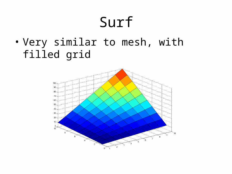
Surf• Very similar to mesh, with filled grid

Contour• Projection of equal heights of 3D plot onto a

2D plane

• Use like surf or mesh – contour(x,y,z)

Meshc,surfc• Combination surface/mesh and contour plot

• Use like surf or mesh – meshc(x,y,z)

Plot3• Plots lines and points in space, just like plot but now for an

(x,y,z) triple• Plot3(x,y,z), each a vector of equal length• Use all the same specfiers to generate colors, line-types,

etc.

Plot commands• Note that almost all 2D plotting commands

such as xlabel, ylabel, title will still work in 3D plots

• 3D plots can be added as subplots just like any other plot type

• Some other special features and functions exist…

View• Changes the view of the current 3D plot

– view(az,el)– Az = azimuth (rotation around z-axis)– El = Elevation (rotation around xy-plane)

• Useful rotations (0,0),(90,0)

Colorbar• For the 3D plots, it is useful to add a

colorbar to the figure to indicate height.

• Colorbar(‘vert’) adds a vertical colorbar

• Colorbar(‘horiz) adds a horizontal colorbar

caxis• Allows you to set the range of colors in the plot. • Caxis([min max]) will choose the range of colors

from the current color map to assign to the plot. Values outside this range will use the min/max available

Colormap• Plenty of other controls to personalize the

plot– colormap colormap_name sets to new map– Colormap (sets the types of colors that appear in 3D

plot). These can be custom of one of several premade– bone Hsv, jet, autumn, vga, summer, …– See help graph3D for more– Use colormapeditor function for graphical selection of

color map

Colormap

Next Week

• Basic Stats / Basic Matlab wrap up

Getting HelpHelp and Documentation

Digital 1. Accessible Help from the Matlab Start Menu

2. Updated online help from the Matlab Mathworks website:

http://www.mathworks.com/access/helpdesk/help/techdoc/matlab.html

3. Matlab command prompt function lookup

4. Built in Demo’s

5. Websites

Hard Copy3. Books, Guides, Reference

The Student Edition of Matlab pub. Mathworks Inc.