MATLAB Tutorial

Steven LevandoskyDepartment of Mathematics

Stanford UniversityCopyright 2001

1

Contents

1 Introduction 3

2 Getting Started 3

3 Variables 4

4 Matrices and Vectors 6

5 Dot Products and Cross Products 9

6 Basic Matrix Operations 11

7 Reduced Row Echelon Form 14

8 Rank 18

9 Inverses 20

10 Eigenvectors and Eigenvalues 23

11 Componentwise Operations 24

12 Plotting Curves 25

13 Plotting Surfaces 28

14 Level Curves 32

15 Vector Fields 34

16 Symbolic Variables and Expressions 36

17 Solving Algebraic Equations 39

18 Derivatives 40

19 M-Files 45

2

1 Introduction

MATLAB, which stands for Matrix Laboratory, is a very powerful program for performingnumerical and symbolic calculations, and is widely used in science and engineering, as well asin mathematics. This tutorial is designed to provide the reader with a basic understanding ofhow MATLAB works, and how to use it to solve problems in linear algebra and multivariablecalculus. It is intended to complement the regular course materials. So, although we oftenrecall many of the basic definitions and results, we assume the reader already has somefamiliarity with them. All of the commands in this document were executed using version5.3, and should also work in version 6.

2 Getting Started

When MATLAB starts (either by typing matlab at the command prompt on a Unix machine,or running the executable on a PC or Mac) the MATLAB prompt

>>

appears. All MATLAB commands are executed from this prompt.

>> 2.3+4.2

ans =

6.5000

By default MATLAB returns numerical expressions as decimals with 5 digits. The format

function is used to change the format of the output. Type format rat to have MATLABreturn rational expressions.

>> format rat

>> 5.1-3.3

ans =

9/5

To eliminate the extra spacing type format compact.

>> format compact

>> 5*7

ans =

35

3

The four basic operations of addition, subtraction, multiplication and division are performedusing the symbols +,-,* and /, respectively. Exponentiation is performed by means of thesymbol ^.

>> 2^7

ans =

128

MATLAB has most standard mathematical functions built-in. The sqrt function computesthe square root.

>> format long

>> sqrt(2)

ans =

1.41421356237310

The basic trigonometric functions (cos, sin, tan, sec, csc, cot), their inverses (acos, asin,atan, asec, acsc, acot), the exponential function exp, and the natural logarithm log arealso built-in. For instance, ln(4) + cos(π/6) is computed as follows.

>> log(4)+cos(pi/6)

ans =

2.25231976490433

For information about any MATLAB function, type help followed by the name of the func-tion.

>> help abs

ABS Absolute value.

ABS(X) is the absolute value of the elements of X. When

X is complex, ABS(X) is the complex modulus (magnitude) of

the elements of X.

See also SIGN, ANGLE, UNWRAP.

Overloaded methods

help sym/abs.m

To avoid having to retype long expressions use the up arrow key ↑ to scroll through linespreviously typed. Typing one or more characters and then the up arrow key displays previouslines that begin with those characters. To exit MATLAB type quit.

3 Variables

To assign a value to a variable in MATLAB simply type the name of the variable, followedby the assignment operator, =, followed by the value.

4

>> x=7

x =

7

Note that variable names in MATLAB are case sensitive, so X and x are not equal. We canperform all of the usual operations with x.

>> x^2-3*x+2

ans =

30

>> log(x)

ans =

1.94591014905531

>> sin(x)

ans =

0.65698659871879

New variables may be defined using existing variables.

>> y=8*x

y =

56

This, however, does not imply any permanent relationship between x and y. If we change x,the value of y does not change.

>> x=x+5

x =

12

>> y

y =

56

The command who returns a list of all variables in the current workspace, while whos returnsthe same list with more detailed information about each variable.

>> who

Your variables are:

ans x y

>> whos

Name Size Bytes Class

ans 1x1 8 double array

x 1x1 8 double array

y 1x1 8 double array

Grand total is 3 elements using 24 bytes

5

Notice that the size of each variable is 1×1. All variables in MATLAB are matrices. Scalarssuch as x and y are just 1 × 1 matrices. We will explain how to enter matrices in the nextsection. To clear one or more variables from the workspace, type clear followed by thenames of the variables. Typing just clear clears all variables.

>> clear

>> who

>> x

??? Undefined function or variable ’x’.

4 Matrices and Vectors

To enter a matrix in MATLAB, use square brackets and separate entries within a row byspaces and separate rows using semicolons.

>> A=[2 1 -1 8; 1 0 8 -3; 7 1 2 4]

A =

2 1 -1 8

1 0 8 -3

7 1 2 4

Often we do not want MATLAB to display a response, especially when dealing with verylarge matrices. To suppress the output, place a semicolon at the end of the line. Typing

>> B=[2 0 -3; -1 1 3];

will still define the variable B containing a 2×3 matrix, but MATLAB will not echo anything.

>> whos

Name Size Bytes Class

A 3x4 96 double array

B 2x3 48 double array

v 3x1 24 double array

Grand total is 21 elements using 168 bytes

To view the contents of the variable B, just type its name.

>> B

B =

2 0 -3

-1 1 3

Vectors (column vectors) are simply matrices with a single column.

6

>> v = [ 2; 3; -4]

v =

2

3

-4

A row vector is a matrix with a single row.

>> w=[3 -2 5 11]

w =

3 -2 5 11

It is often necessary to define vectors with evenly spaced entries. In MATLAB, the colon(:) provides a shorthand for creating such vectors.

>> 2:5

ans =

2 3 4 5

Typing j:i:k defines a row vector with increment i starting at j and ending at k.

>> 3:2:9

ans =

3 5 7 9

Recall that the transpose of a matrix A is the matrix AT whose entry in row i column j isthe same as the entry in row j column i of A. In MATLAB, A’ represents the transpose ofthe matrix A.

>> A=[5 -2 9; 11 7 8]

A =

5 -2 9

11 7 8

>> A’

ans =

5 11

-2 7

9 8

To define regularly spaced column vectors, we can take the transpose of a regularly spacedrow vector.

>> [1:3:10]’

ans =

1

4

7

10

7

The entry in row i, column j of a matrix A is A(i,j).

>> A=[3 -2 7 8; 4 3 2 1; 10 15 -2 9]

A =

3 -2 7 8

4 3 2 1

10 15 -2 9

>> A(3,2)

ans =

15

It is also possible to view multiple entries within any row or column. For instance, the secondand fourth entries in the third row are accessed as follows.

>> A(3,[2 4])

ans =

15 9

Row i of A is A(i,:) and column j of A is A(:,j).

>> A(3,:)

ans =

10 15 -2 9

>> A(:,3)

ans =

7

2

-2

Next we display the first, second and fourth columns.

>> A(:,[1 2 4])

ans =

3 -2 8

4 3 1

10 15 9

The entries of a vector (row or column) may be accessed using a single index.

>> w=[7; 13; 11]

w =

7

13

11

>> w(2)

ans =

13

8

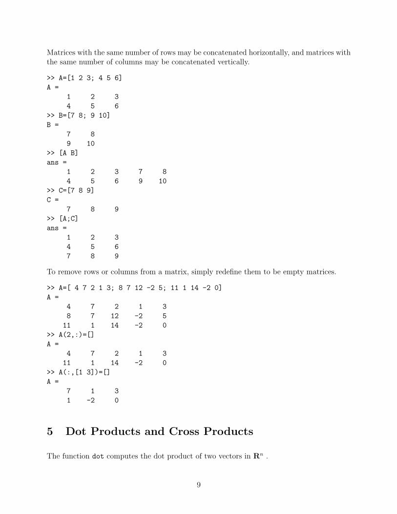
Matrices with the same number of rows may be concatenated horizontally, and matrices withthe same number of columns may be concatenated vertically.

>> A=[1 2 3; 4 5 6]

A =

1 2 3

4 5 6

>> B=[7 8; 9 10]

B =

7 8

9 10

>> [A B]

ans =

1 2 3 7 8

4 5 6 9 10

>> C=[7 8 9]

C =

7 8 9

>> [A;C]

ans =

1 2 3

4 5 6

7 8 9

To remove rows or columns from a matrix, simply redefine them to be empty matrices.

>> A=[ 4 7 2 1 3; 8 7 12 -2 5; 11 1 14 -2 0]

A =

4 7 2 1 3

8 7 12 -2 5

11 1 14 -2 0

>> A(2,:)=[]

A =

4 7 2 1 3

11 1 14 -2 0

>> A(:,[1 3])=[]

A =

7 1 3

1 -2 0

5 Dot Products and Cross Products

The function dot computes the dot product of two vectors in Rn .

9

>> v=[7; 23; 15; 2], w=[5; -2; 1; -8]

v =

7

23

15

2

w =

5

-2

1

-8

>> dot(v,w)

ans =

-12

Note that the dot product is symmetric.

>> dot(w,v)

ans =

-12

Recall that the length of a vector v is ‖v‖ =√

v · v.

>> vlength=sqrt(dot(v,v))

vlength =

28.4077

The length of a vector can also be found directly using the norm function.

>> norm(v)

ans =

28.4077

Also recall that if θ is the angle between two vectors v and w then v · w = ‖v‖‖w‖ cos θ.Solving for the angle we have θ = arccos((v ·w)/‖v‖‖w‖).>> theta=acos(dot(v,w)/(norm(v)*norm(w)))

theta =

1.6144

>> theta*180/pi

ans =

92.4971

So the angle between v and w is about 92.5◦.The function cross computes the cross product of two vectors in R3.

>> v=[3; 2; 1], w=[4; 15; 1]

v =

10

3

2

1

w =

4

15

1

>> x=cross(v,w)

x =

-13

1

37

Cross products are anti-symmetric. That is, w × v = −v ×w.

>> cross(w,v)

ans =

13

-1

-37

The cross product v × w is orthogonal to both v and w. We can verify this by taking itsdot product with both v and w. Recall that two vectors are orthogonal if and only if theirdot product equals zero.

>> dot(x,v)

ans =

0

>> dot(x,w)

ans =

0

6 Basic Matrix Operations

Addition (and subtraction) of matrices of the same dimensions is performed componentwise.

>> A=[5 -1 2; 3 4 7]

A =

5 -1 2

3 4 7

>> B=[2 2 1; 5 0 3]

B =

2 2 1

5 0 3

>> A+B

11

ans =

7 1 3

8 4 10

Note that only matrices with the same dimensions may be summed.

>> C=[3 1; 6 4]

C =

3 1

6 4

>> A+C

??? Error using ==> +

Matrix dimensions must agree.

Scalar multiplication (and division by nonzero scalars) is also performed componentwise.

>> 2*A

ans =

10 -2 4

6 8 14

The * in scalar multiplication is not optional.

>> 2A

??? 2

|

Missing operator, comma, or semi-colon.

Vector addition and scalar multiplication are performed in the same way.

>> v=[3; 5], w=[-2; 7]

v =

3

5

w =

-2

7

>> 10*v-5*w

ans =

40

15

The matrix product A*B is defined when A is m× n and B is n× k. That is, the number ofcolumns of A must equal the number of rows of A. In this case the product A*B is an m× kmatrix.

>> A=[3 1 7 2; 6 -3 4 2; 9 4 -1 -2]

A =

12

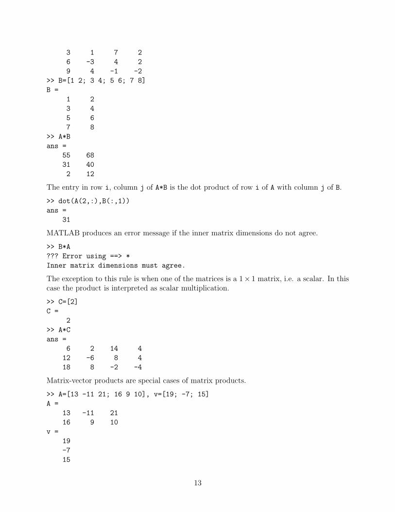
3 1 7 2

6 -3 4 2

9 4 -1 -2

>> B=[1 2; 3 4; 5 6; 7 8]

B =

1 2

3 4

5 6

7 8

>> A*B

ans =

55 68

31 40

2 12

The entry in row i, column j of A*B is the dot product of row i of A with column j of B.

>> dot(A(2,:),B(:,1))

ans =

31

MATLAB produces an error message if the inner matrix dimensions do not agree.

>> B*A

??? Error using ==> *

Inner matrix dimensions must agree.

The exception to this rule is when one of the matrices is a 1× 1 matrix, i.e. a scalar. In thiscase the product is interpreted as scalar multiplication.

>> C=[2]

C =

2

>> A*C

ans =

6 2 14 4

12 -6 8 4

18 8 -2 -4

Matrix-vector products are special cases of matrix products.

>> A=[13 -11 21; 16 9 10], v=[19; -7; 15]

A =

13 -11 21

16 9 10

v =

19

-7

15

13

>> A*v

ans =

639

391

As above, the entries of A*v are the dot products of the rows of A with v.

>> [dot(A(1,:),v); dot(A(2,:),v)]

ans =

639

391

Also, the product A*v equals the linear combination of the columns of A whose coefficientsare the components of v.

>> v(1)*A(:,1)+v(2)*A(:,2)+v(3)*A(:,3)

ans =

639

391

A square matrix may be multiplied by itself, and in this case it makes sense to take powersof the matrix. For instance, A^6 equals A*A*A*A*A*A.

>> A=[0 1; 1 1]

A =

0 1

1 1

>> A*A

ans =

1 1

1 2

>> A^6

ans =

5 8

8 13

7 Reduced Row Echelon Form

The rref command is used to compute the reduced row echelon form of a matrix.

>> A=[1 2 3 4 5 6; 1 2 4 8 16 32; 2 4 2 4 2 4; 1 2 1 2 1 2]

A =

1 2 3 4 5 6

1 2 4 8 16 32

2 4 2 4 2 4

1 2 1 2 1 2

14

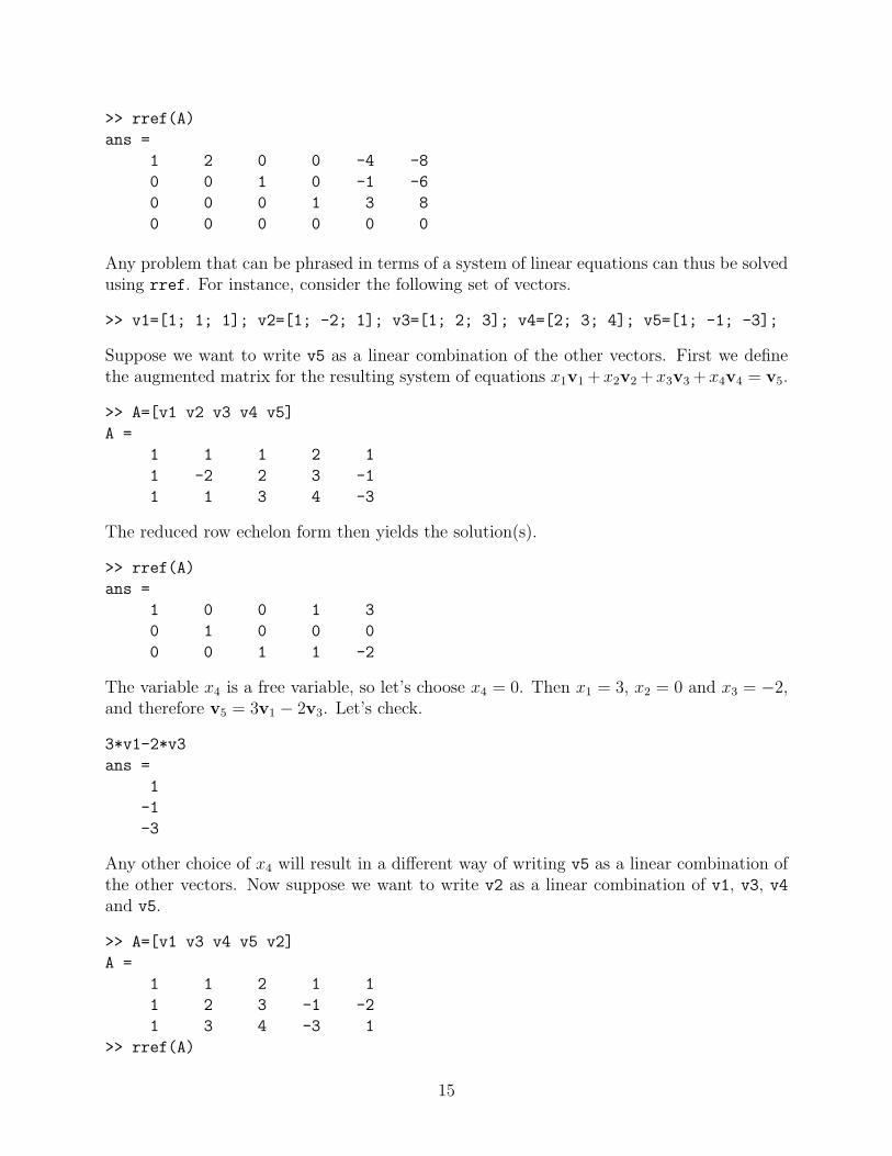
>> rref(A)

ans =

1 2 0 0 -4 -8

0 0 1 0 -1 -6

0 0 0 1 3 8

0 0 0 0 0 0

Any problem that can be phrased in terms of a system of linear equations can thus be solvedusing rref. For instance, consider the following set of vectors.

>> v1=[1; 1; 1]; v2=[1; -2; 1]; v3=[1; 2; 3]; v4=[2; 3; 4]; v5=[1; -1; -3];

Suppose we want to write v5 as a linear combination of the other vectors. First we definethe augmented matrix for the resulting system of equations x1v1 +x2v2 +x3v3 +x4v4 = v5.

>> A=[v1 v2 v3 v4 v5]

A =

1 1 1 2 1

1 -2 2 3 -1

1 1 3 4 -3

The reduced row echelon form then yields the solution(s).

>> rref(A)

ans =

1 0 0 1 3

0 1 0 0 0

0 0 1 1 -2

The variable x4 is a free variable, so let’s choose x4 = 0. Then x1 = 3, x2 = 0 and x3 = −2,and therefore v5 = 3v1 − 2v3. Let’s check.

3*v1-2*v3

ans =

1

-1

-3

Any other choice of x4 will result in a different way of writing v5 as a linear combination ofthe other vectors. Now suppose we want to write v2 as a linear combination of v1, v3, v4and v5.

>> A=[v1 v3 v4 v5 v2]

A =

1 1 2 1 1

1 2 3 -1 -2

1 3 4 -3 1

>> rref(A)

15

ans =

1 0 1 3 0

0 1 1 -2 0

0 0 0 0 1

This time the third equation reduces to 0 = 1, so there are no solutions, and therefore v2 isnot a linear combination of the other vectors.

Another way to use rref is in the form [R,p]=rref(A), which defines R to be the reducedrow echelon form of A and p to be the vector listing the columns of R which contain pivots.

>> A=[ 1 2 1 5; 1 2 2 6; 1 2 3 7; 1 2 4 8]

A =

1 2 1 5

1 2 2 6

1 2 3 7

1 2 4 8

>> [R,p]=rref(A)

R =

1 2 0 4

0 0 1 1

0 0 0 0

0 0 0 0

p =

1 3

Extracting the pivot columns of A gives a basis for the column space of A.

>> A(:,p)

ans =

1 1

1 2

1 3

1 4

With the reduced row echelon form of A in hand we could easily find a basis for the nullspace of A. The command null does this for us.

>> null(A,’r’)

ans =

-2 -4

1 0

0 -1

0 1

The ’r’ stands for rational and tells MATLAB to find the null space from the reduced rowechelon form of A. Without the ’r’, MATLAB finds an orthonormal basis for the null space— that is, a basis consisting of mutually orthogonal unit vectors.

16

>> N=null(A)

N =

-0.9608 0

0.1601 -0.8165

-0.1601 -0.4082

0.1601 0.4082

To verify that this is an orthonormal basis we form the product N’*N. Since the rows of N’are the columns of N, the entry in row i, column j of N’*N is the dot product of column i

and column j of N.

>> N’*N

ans =

1.0000 0

0 1.0000

The ones on the diagonal indicate that the columns of N are unit vectors, and the zerosindicate that they are orthogonal to each other.

We can also use rref to find the inverse of an invertible matrix. Recall that a matrixA is invertible if and only if rref(A) = In, the n × n identity matrix, and that in this caserref [A | In] = [In | A−1]. For example, consider the following matrix.

>> A=[1 1 1; 1 2 3; 1 3 6]

A =

1 1 1

1 2 3

1 3 6

In MATLAB, the n× n identity matrix In is given by eye(n). Let’s augment A by eye(3)

and compute its reduced row echelon form.

>> B=[A eye(3)]

B =

1 1 1 1 0 0

1 2 3 0 1 0

1 3 6 0 0 1

>> rref(B)

ans =

1 0 0 3 -3 1

0 1 0 -3 5 -2

0 0 1 1 -2 1

So

>> Ainv=[3 -3 1; -3 5 -2; 1 -2 1]

Ainv =

3 -3 1

-3 5 -2

1 -2 1

17

is the inverse of A. To verify this, recall that A−1A = AA−1 = In.

>> Ainv*A

ans =

1 0 0

0 1 0

0 0 1

>> A*Ainv

ans =

1 0 0

0 1 0

0 0 1

8 Rank

To compute the rank of a matrix we use the rank command. We briefly recall some of theimportant facts regarding the rank of a matrix.

• The rank of a matrix equals the dimension of its column space.

• The columns of a matrix are linearly independent if and only if its rank equals thenumber of columns.

• An n× n square matrix is invertible if and only if its rank equals n.

For example,

>> A=[1 2 1 4; 2 3 1 3; 3 2 1 2; 4 3 1 1]

A =

1 2 1 4

2 3 1 3

3 2 1 2

4 3 1 1

>> rank(A)

ans =

3

Thus the column space of A has dimension 3 and the columns of A above are linearly de-pendent. Using rank we can determine which columns of A form a basis for its columnspace.

>> rank(A(:,[1 2 3]))

ans =

3

>> rank(A(:,[1 2 4]))

ans =

18

3

>> rank(A(:,[1 3 4]))

ans =

2

>> rank(A(:,[2 3 4]))

ans =

3

Thus any choice of three columns forms a basis for the column space of A except columnsone, three and four. Next we use rank as a test for invertibility.

>> A=[11 -21 3; 8 2 1; 16 -12 5]

A =

11 -21 3

8 2 1

16 -12 5

>> rank(A)

ans =

3

>> B=[3 4 5;6 7 8;9 10 11]

B =

3 4 5

6 7 8

9 10 11

>> rank(B)

ans =

2

The matrix A is invertible, but B is not.Using rank it is possible to determine whether or not a given vector is in the column

space of a matrix.

>> A=[5 8 -4; 3 19 11; -6 6 0; 12 4 1]

A =

5 8 -4

3 19 11

-6 6 0

12 4 1

>> v1=[21; 16; -7; 33],v2=[30; 7; 30; -16]

v1 =

21

16

-7

33

v2 =

19

30

7

30

-16

>> rank(A)

ans =

3

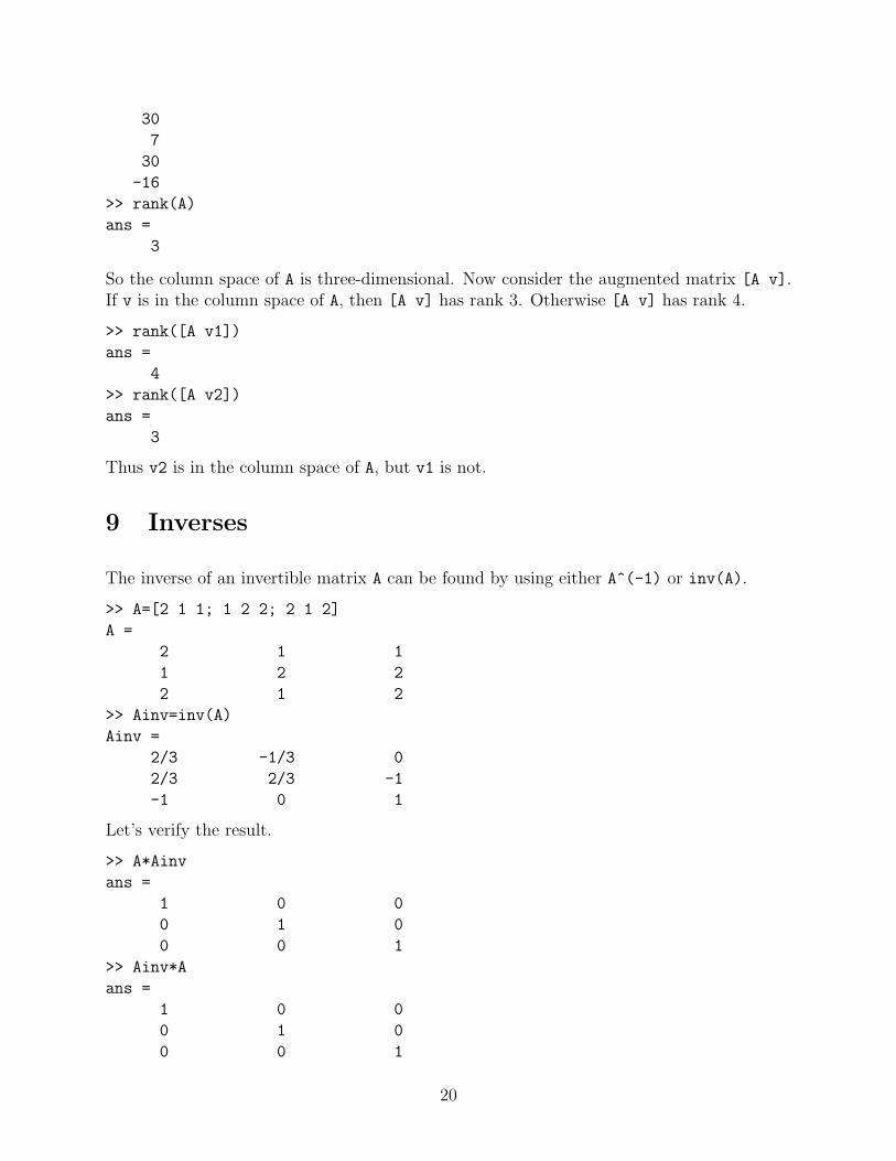
So the column space of A is three-dimensional. Now consider the augmented matrix [A v].If v is in the column space of A, then [A v] has rank 3. Otherwise [A v] has rank 4.

>> rank([A v1])

ans =

4

>> rank([A v2])

ans =

3

Thus v2 is in the column space of A, but v1 is not.

9 Inverses

The inverse of an invertible matrix A can be found by using either A^(-1) or inv(A).

>> A=[2 1 1; 1 2 2; 2 1 2]

A =

2 1 1

1 2 2

2 1 2

>> Ainv=inv(A)

Ainv =

2/3 -1/3 0

2/3 2/3 -1

-1 0 1

Let’s verify the result.

>> A*Ainv

ans =

1 0 0

0 1 0

0 0 1

>> Ainv*A

ans =

1 0 0

0 1 0

0 0 1

20

MATLAB gives a warning message if the matrix is singular (not invertible).

>> B=[1 2 3;4 5 6;7 8 9]

B =

1 2 3

4 5 6

7 8 9

>> inv(B)

Warning: Matrix is close to singular or badly scaled.

Results may be inaccurate. RCOND = 2.055969e-018.

ans =

1.0e+016 *

-0.4504 0.9007 -0.4504

0.9007 -1.8014 0.9007

-0.4504 0.9007 -0.4504

Here MATLAB actually returns an inverse. To see that B is really singular, compute itsrank.

>> rank(B)

ans =

2

Since the rank of B is less than 3, B is singular. Also recall that a matrix is invertible if andonly if its determinant is nonzero.

>> det(B)

ans =

0

Unfortunately, there are invertible matrices which MATLAB regards as singular.

>> format long

>> C=[1.00000000000001 1; 1 .99999999999999]

C =

1.00000000000001 1.00000000000000

1.00000000000000 0.99999999999999

>> inv(C)

Warning: Matrix is singular to working precision.

ans =

Inf Inf

Inf Inf

>> rank(C)

ans =

1

>> det(C)

ans =

21

0

>> rref(C)

ans =

1.00000000000000 0.99999999999999

0 0

According to MATLAB, the matrix C has rank 1 and determinant zero, and is thereforesingular. However, if we let ε = 0.00000000000001, then det(C) = (1+ε)(1−ε)−1 = −ε2 6= 0,so C is invertible. The problem is that in format long MATLAB is accurate to 15 placesand therefore recognizes 1 + ε and 1− ε as being different from 1, but recognizes

(1 + ε)(1− ε) = 1− ε2 = 0.9999999999999999999999999999

as 1. This example should serve as a warning to not blindly accept everything that MATLABtells us.

To solve an equation of the form Ax = b where A is invertible, we simply multiply bythe inverse of A to get x = A−1b.

>> A=[11 7 -6 8; 3 -1 12 15; 1 1 1 7; -4 6 1 8]

A =

11 7 -6 8

3 -1 12 15

1 1 1 7

-4 6 1 8

>> b=[10; -23; -13; 4]

b =

10

-23

-13

4

>> format rat

>> x=inv(A)*b

x =

1

5

2

-3

Let’s verify this result.

>> A*x

ans =

10

-23

-13

4

22

10 Eigenvectors and Eigenvalues

The eig command is used to find the eigenvalues of a square matrix.

>> A=[ 3 1 1; 1 3 1; 1 1 3]

A =

3 1 1

1 3 1

1 1 3

>> eig(A)

ans =

2.0000

2.0000

5.0000

If A is diagonalizable, the eig command can also be used to find an eigenbasis, along withthe diagonal matrix to which it is similar.

>> [Q,D]=eig(A)

Q =

-0.8164 -0.0137 0.5774

0.3963 0.7139 0.5774

0.4201 -0.7001 0.5774

D =

2.0000 0 0

0 2.0000 0

0 0 5.0000

Here, the columns of the matrix Q form an eigenbasis of A, and Q−1AQ = D. Let’s check.

>> inv(Q)*A*Q

ans =

2.0000 0 0.0000

0.0000 2.0000 0.0000

-0.0000 0.0000 5.0000

The matrix Q actually contains an orthonormal basis of eigenvectors.

>> Q’*Q

ans =

1.0000 0.0000 -0.0000

0.0000 1.0000 -0.0000

-0.0000 -0.0000 1.0000

If we just wanted to find the eigenvectors in the “usual” way, we would use the null com-mand.

23

>> C1=null(A-2*eye(3),’r’)

C1 =

-1 -1

1 0

0 1

>> C2=null(A-5*eye(3),’r’)

C2 =

1

1

1

Let’s now check that these three vectors form an eigenbasis.

>> C=[C1 C2]

C =

-1 -1 1

1 0 1

0 1 1

>> inv(C)*A*C

ans =

2.0000 -0.0000 0.0000

0 2.0000 -0.0000

0 0 5.0000

Great! It worked.

11 Componentwise Operations

The componentwise product of two matrices A and B is the matrix A.*B whose entries arethe products of the corresponding entries of A and B.

>> A=[ 1 2 3; 4 5 6]

A =

1 2 3

4 5 6

>> B=[ 3 2 1; -1 2 2]

B =

3 2 1

-1 2 2

>> A.*B

ans =

3 4 3

-4 10 12

Componentwise division and exponentiation are defined by A./B and A.^B, respectively.Each componentwise operation must make sense, or MATLAB will produce an error message.

24

>> A./B

ans =

1/3 1 3

-4 5/2 3

>> A.^B

ans =

1 4 3

1/4 25 36

12 Plotting Curves

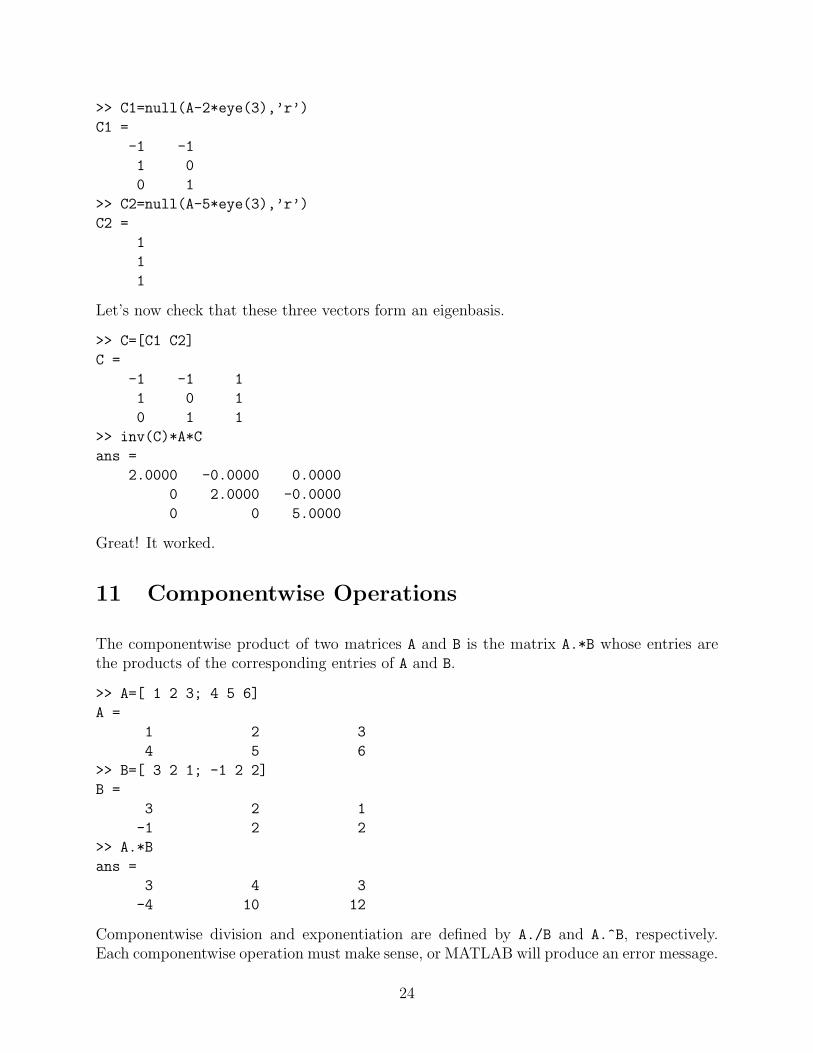
The plot function is used to plot data in the plane. Given a vector x of x-coordinates x1

through xn and a vector y of y-coordinates y1 through yn, plot(x,y) graphs the points(x1, y1) through (xn, yn). By default these points are connected in order by straight linesegments. For example, here is how one would plot the quadrilateral with vertices (0, 0),(1, 1), (4, 2) and (5,−1).

>> x=[0 1 4 5 0];

>> y=[0 1 2 -1 0];

>> plot(x,y)

0 0.5 1 1.5 2 2.5 3 3.5 4 4.5 5−1

−0.5

0

0.5

1

1.5

2

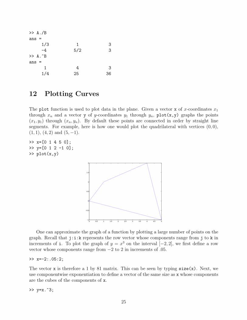
One can approximate the graph of a function by plotting a large number of points on thegraph. Recall that j:i:k represents the row vector whose components range from j to k inincrements of i. To plot the graph of y = x3 on the interval [−2, 2], we first define a rowvector whose components range from −2 to 2 in increments of .05.

>> x=-2:.05:2;

The vector x is therefore a 1 by 81 matrix. This can be seen by typing size(x). Next, weuse componentwise exponentiation to define a vector of the same size as x whose componentsare the cubes of the components of x.

>> y=x.^3;

25

Typing y=x^3 would result in an error since x is not a square matrix. Finally we use theplot function to display the graph.

>> plot(x,y)

Now let’s give our figure a title.

>> title(’Graph of f(x)=x^3’)

−2 −1.5 −1 −0.5 0 0.5 1 1.5 2−8

−6

−4

−2

0

2

4

6

8Graph of f(x)=x3

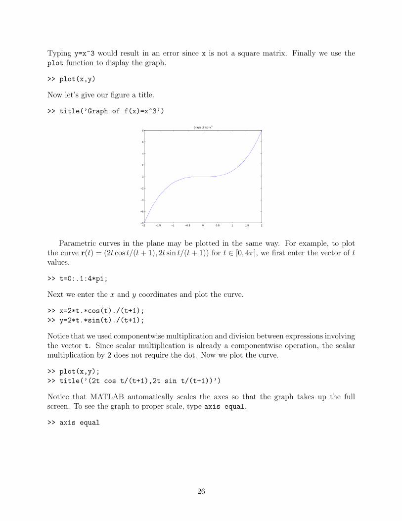
Parametric curves in the plane may be plotted in the same way. For example, to plotthe curve r(t) = (2t cos t/(t + 1), 2t sin t/(t + 1)) for t ∈ [0, 4π], we first enter the vector of tvalues.

>> t=0:.1:4*pi;

Next we enter the x and y coordinates and plot the curve.

>> x=2*t.*cos(t)./(t+1);

>> y=2*t.*sin(t)./(t+1);

Notice that we used componentwise multiplication and division between expressions involvingthe vector t. Since scalar multiplication is already a componentwise operation, the scalarmultiplication by 2 does not require the dot. Now we plot the curve.

>> plot(x,y);

>> title(’(2t cos t/(t+1),2t sin t/(t+1))’)

Notice that MATLAB automatically scales the axes so that the graph takes up the fullscreen. To see the graph to proper scale, type axis equal.

>> axis equal

26

−2 −1.5 −1 −0.5 0 0.5 1 1.5 2

−1.5

−1

−0.5

0

0.5

1

1.5

(2t cos t/(t+1),2t sin t/(t+1))

To plot more than one curve in the same figure, type hold on. For instance, let’s plotthe two circles x2 + y2 = 4 and (x− 1)2 +(y− 1)2 = 1. These are parametrized, respectively,by r1(t) = (2 cos t, 2 sin t) and r2(t) = (1 + cos t, 1 + sin t) for t ∈ [0, 2π].

>> t=0:pi/20:2*pi;

>> plot(2*cos(t),2*sin(t))

>> hold on

>> plot(1+cos(t),1+sin(t))

>> axis equal

>> title(’The circles x^2+y^2=4 and (x-1)^2+(y-1)^2=1’)

−2.5 −2 −1.5 −1 −0.5 0 0.5 1 1.5 2 2.5−2

−1.5

−1

−0.5

0

0.5

1

1.5

2The circles x2+y2=4 and (x−1)2+(y−1)2=1

The three dimensional analogue of plot is plot3. For example, the parametric curver(t) = (cos(t), sin(t), t) for t ∈ [0, 8π] is plotted as follows.

>> t=0:.1:8*pi;

>> plot3(cos(t),sin(t),t)

>> title(’(cos t,sin t,t)’)

27

−1

−0.5

0

0.5

1

−1

−0.5

0

0.5

10

5

10

15

20

25

30

(cos t,sin t,t)

13 Plotting Surfaces

To plot the graph of a function f(x, y) over a rectangular domain

R = [a, b]× [c, d] = {(x, y) | a ≤ x ≤ b and c ≤ y ≤ d},

we need to first create a grid of points within the domain using the function meshgrid.

0 1 2 3 40

3

2

1

For example, to subdivide the rectangle [0, 4] × [0, 3] into rectangles of width 1 and height.5, we first define vectors x and y which determine the spacing of the grid.

>> x=0:4

x =

0 1 2 3 4

>> y=0:.5:3

y =

0 0.5000 1.0000 1.5000 2.0000 2.5000 3.0000

Next meshgrid defines the points in the grid.

28

>> [X,Y]=meshgrid(x,y)

X =

0 1 2 3 4

0 1 2 3 4

0 1 2 3 4

0 1 2 3 4

0 1 2 3 4

0 1 2 3 4

0 1 2 3 4

Y =

0 0 0 0 0

0.5000 0.5000 0.5000 0.5000 0.5000

1.0000 1.0000 1.0000 1.0000 1.0000

1.5000 1.5000 1.5000 1.5000 1.5000

2.0000 2.0000 2.0000 2.0000 2.0000

2.5000 2.5000 2.5000 2.5000 2.5000

3.0000 3.0000 3.0000 3.0000 3.0000

These 7×5 matrices define the 35 points in the grid. The matrix X contains the x coordinatesand Y contains the y coordinates. Suppose now that we want to plot the function f(x, y) =3x− 2y. We then define the matrix Z of z coordinates.

>> Z=3*X-2*Y

Z =

0 3 6 9 12

-1 2 5 8 11

-2 1 4 7 10

-3 0 3 6 9

-4 -1 2 5 8

-5 -2 1 4 7

-6 -3 0 3 6

Finally, we use surf to plot the surface.

>> surf(X,Y,Z)

>> title(’Graph of f(x,y)=3x-2y’)

0

1

2

3

4

0

0.5

1

1.5

2

2.5

3−6

−4

−2

0

2

4

6

8

10

12

Graph of f(x,y)=3x−2y

29

It was actually not necessary in this example to define the variables x and y. We could havedefined the grid directly by typing

>> [X,Y]=meshgrid(0:4,0:.5:3)

Also, if meshgrid is provided a single vector as its argument, it defines a square grid with thesame spacing in x and y. So meshgrid(0:.5:2) is equivalent to meshgrid(0:.5:2,0.5:2).

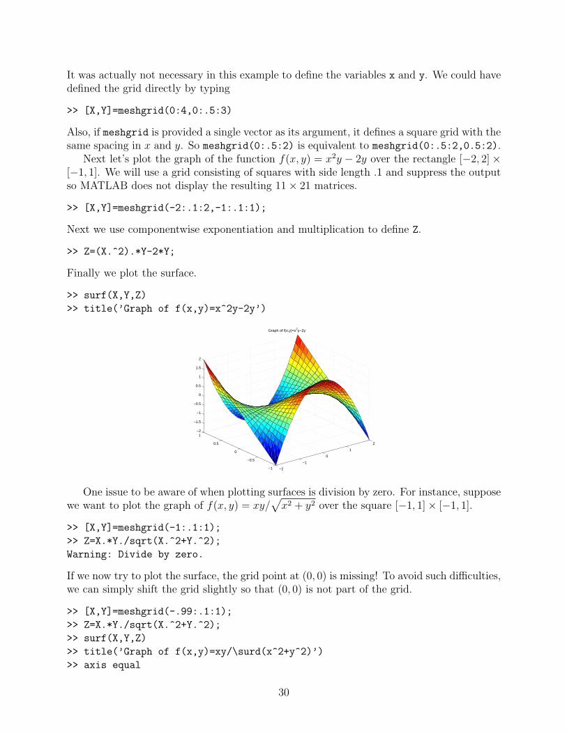
Next let’s plot the graph of the function f(x, y) = x2y − 2y over the rectangle [−2, 2]×[−1, 1]. We will use a grid consisting of squares with side length .1 and suppress the outputso MATLAB does not display the resulting 11× 21 matrices.

>> [X,Y]=meshgrid(-2:.1:2,-1:.1:1);

Next we use componentwise exponentiation and multiplication to define Z.

>> Z=(X.^2).*Y-2*Y;

Finally we plot the surface.

>> surf(X,Y,Z)

>> title(’Graph of f(x,y)=x^2y-2y’)

−2

−1

0

1

2

−1

−0.5

0

0.5

1−2

−1.5

−1

−0.5

0

0.5

1

1.5

2

Graph of f(x,y)=x2y−2y

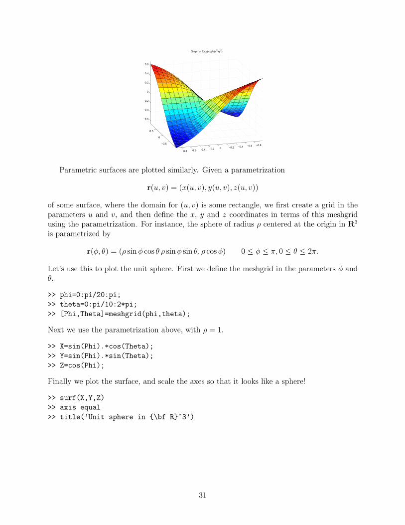
One issue to be aware of when plotting surfaces is division by zero. For instance, supposewe want to plot the graph of f(x, y) = xy/

√x2 + y2 over the square [−1, 1]× [−1, 1].

>> [X,Y]=meshgrid(-1:.1:1);

>> Z=X.*Y./sqrt(X.^2+Y.^2);

Warning: Divide by zero.

If we now try to plot the surface, the grid point at (0, 0) is missing! To avoid such difficulties,we can simply shift the grid slightly so that (0, 0) is not part of the grid.

>> [X,Y]=meshgrid(-.99:.1:1);

>> Z=X.*Y./sqrt(X.^2+Y.^2);

>> surf(X,Y,Z)

>> title(’Graph of f(x,y)=xy/\surd(x^2+y^2)’)

>> axis equal

30

−0.5

0

0.5

−0.8−0.6−0.4−0.200.20.40.60.8

−0.6

−0.4

−0.2

0

0.2

0.4

0.6

Graph of f(x,y)=xy/√(x2+y2)

Parametric surfaces are plotted similarly. Given a parametrization

r(u, v) = (x(u, v), y(u, v), z(u, v))

of some surface, where the domain for (u, v) is some rectangle, we first create a grid in theparameters u and v, and then define the x, y and z coordinates in terms of this meshgridusing the parametrization. For instance, the sphere of radius ρ centered at the origin in R3

is parametrized by

r(φ, θ) = (ρ sin φ cos θ ρ sin φ sin θ, ρ cos φ) 0 ≤ φ ≤ π, 0 ≤ θ ≤ 2π.

Let’s use this to plot the unit sphere. First we define the meshgrid in the parameters φ andθ.

>> phi=0:pi/20:pi;

>> theta=0:pi/10:2*pi;

>> [Phi,Theta]=meshgrid(phi,theta);

Next we use the parametrization above, with ρ = 1.

>> X=sin(Phi).*cos(Theta);

>> Y=sin(Phi).*sin(Theta);

>> Z=cos(Phi);

Finally we plot the surface, and scale the axes so that it looks like a sphere!

>> surf(X,Y,Z)

>> axis equal

>> title(’Unit sphere in {\bf R}^3’)

31

−1

−0.5

0

0.5

1

−1

−0.5

0

0.5

1−1

−0.5

0

0.5

1

Unit sphere in R3

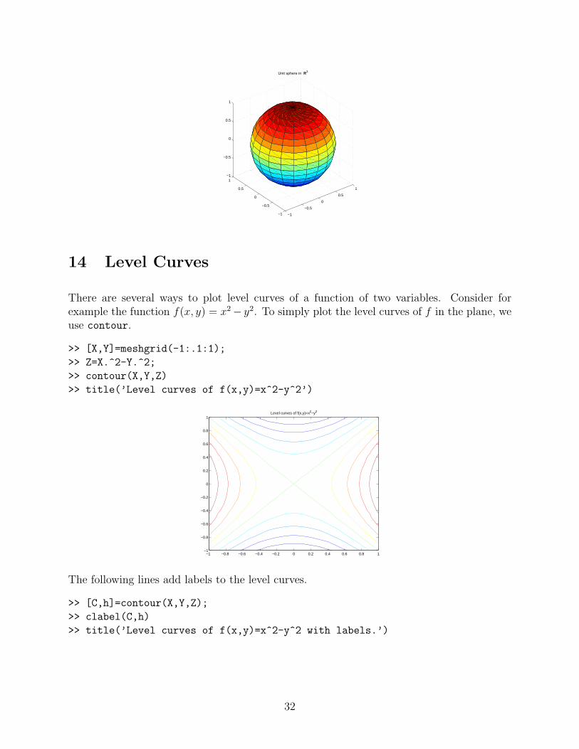
14 Level Curves

There are several ways to plot level curves of a function of two variables. Consider forexample the function f(x, y) = x2− y2. To simply plot the level curves of f in the plane, weuse contour.

>> [X,Y]=meshgrid(-1:.1:1);

>> Z=X.^2-Y.^2;

>> contour(X,Y,Z)

>> title(’Level curves of f(x,y)=x^2-y^2’)

−1 −0.8 −0.6 −0.4 −0.2 0 0.2 0.4 0.6 0.8 1−1

−0.8

−0.6

−0.4

−0.2

0

0.2

0.4

0.6

0.8

1Level curves of f(x,y)=x2−y2

The following lines add labels to the level curves.

>> [C,h]=contour(X,Y,Z);

>> clabel(C,h)

>> title(’Level curves of f(x,y)=x^2-y^2 with labels.’)

32

−1 −0.8 −0.6 −0.4 −0.2 0 0.2 0.4 0.6 0.8 1−1

−0.8

−0.6

−0.4

−0.2

0

0.2

0.4

0.6

0.8

1Level curves of f(x,y)=x2−y2 with labels.

−0.8 −0.8

−0.8 −0.8

−0.6−0.6

−0.6

−0.6

−0.4

−0.4

−0.4

−0.4

−0.4

−0.4

−0.2

−0.2−0.2

−0.2

−0.2−0.2

0

0

0

0

0

0

0

0

0.2

0.2

0.2

0.2

0.2

0.2

0.4

0.4

0.4

0.4

0.4

0.4

0.6

0.6

0.6

0.6

0.8 0.8

To show the level curves in R3 at their actual height, use contour3.

>> contour3(X,Y,Z)

>> title(’Level curves of f(x,y)=x^2-y^2 at actual height.’)

−1

−0.5

0

0.5

1

−1

−0.5

0

0.5

1−0.8

−0.6

−0.4

−0.2

0

0.2

0.4

0.6

0.8

Level curves of f(x,y)=x2−y2 at actual height.

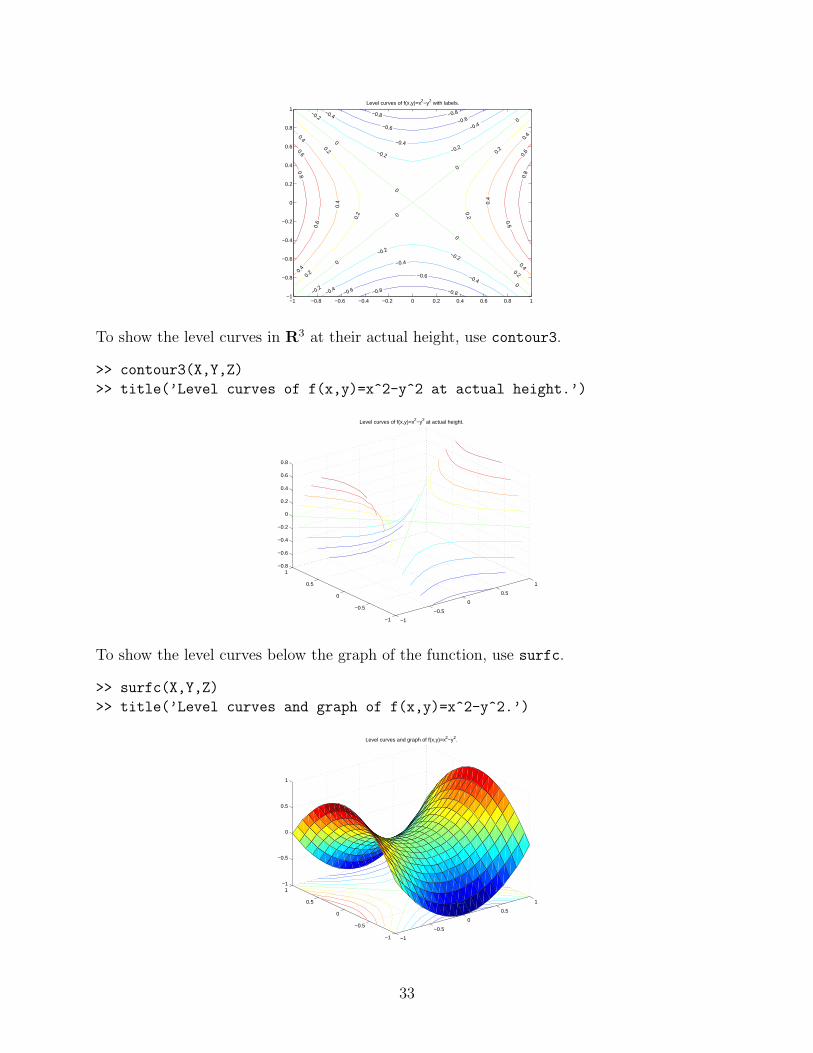
To show the level curves below the graph of the function, use surfc.

>> surfc(X,Y,Z)

>> title(’Level curves and graph of f(x,y)=x^2-y^2.’)

−1

−0.5

0

0.5

1

−1

−0.5

0

0.5

1−1

−0.5

0

0.5

1

Level curves and graph of f(x,y)=x2−y2.

33

15 Vector Fields

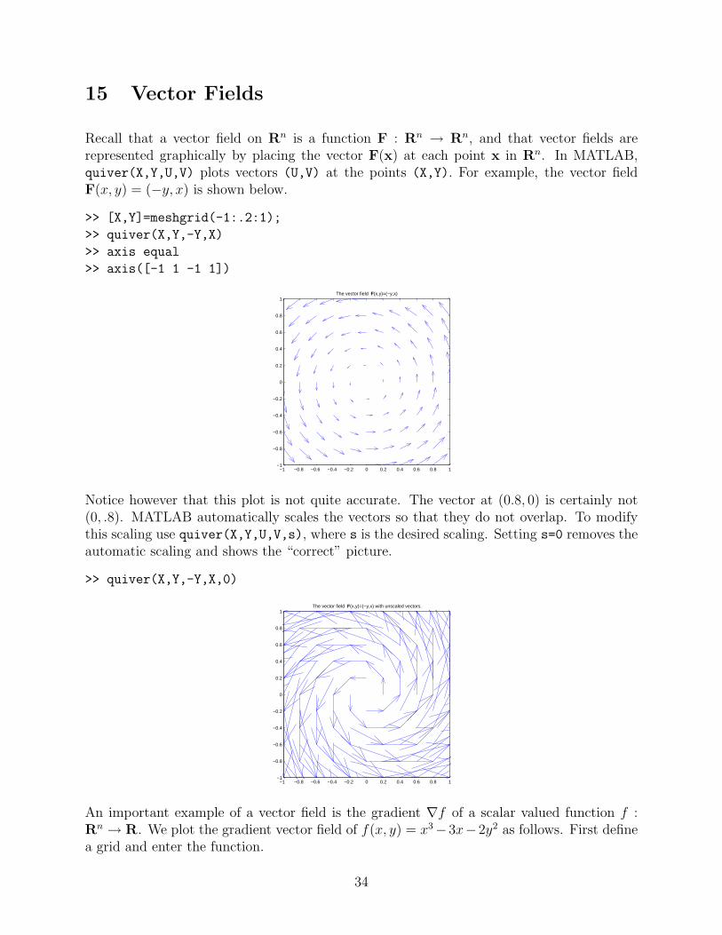
Recall that a vector field on Rn is a function F : Rn → Rn, and that vector fields arerepresented graphically by placing the vector F(x) at each point x in Rn. In MATLAB,quiver(X,Y,U,V) plots vectors (U,V) at the points (X,Y). For example, the vector fieldF(x, y) = (−y, x) is shown below.

>> [X,Y]=meshgrid(-1:.2:1);

>> quiver(X,Y,-Y,X)

>> axis equal

>> axis([-1 1 -1 1])

−1 −0.8 −0.6 −0.4 −0.2 0 0.2 0.4 0.6 0.8 1−1

−0.8

−0.6

−0.4

−0.2

0

0.2

0.4

0.6

0.8

1The vector field F(x,y)=(−y,x)

Notice however that this plot is not quite accurate. The vector at (0.8, 0) is certainly not(0, .8). MATLAB automatically scales the vectors so that they do not overlap. To modifythis scaling use quiver(X,Y,U,V,s), where s is the desired scaling. Setting s=0 removes theautomatic scaling and shows the “correct” picture.

>> quiver(X,Y,-Y,X,0)

−1 −0.8 −0.6 −0.4 −0.2 0 0.2 0.4 0.6 0.8 1−1

−0.8

−0.6

−0.4

−0.2

0

0.2

0.4

0.6

0.8

1The vector field F(x,y)=(−y,x) with unscaled vectors.

An important example of a vector field is the gradient ∇f of a scalar valued function f :Rn → R. We plot the gradient vector field of f(x, y) = x3−3x−2y2 as follows. First definea grid and enter the function.

34

>> [X,Y]=meshgrid(-2:.2:2,-1:.2:1);

>> Z=X.^3-3*X-2*Y.^2;

Next,

[DX,DY]=gradient(Z,.2,.2);

defines [DX,DY] to be (approximately) the gradient of f . The crucial thing here is that thesecond and third arguments agree with the spacing in the previous meshgrid. Finally, weuse quiver to plot the field.

>> quiver(X,Y,DX,DY)

>> axis equal

>> axis([-2 2 -1 1])

>> title(’Gradient vector field of f(x,y)=x^3-3x-2y^2’)

−2 −1.5 −1 −0.5 0 0.5 1 1.5 2−1

−0.8

−0.6

−0.4

−0.2

0

0.2

0.4

0.6

0.8

1Gradient vector field of f(x,y)=x3−3x−2y2

Now let’s plot the level curves of f on the same plot. Using a finer grid makes the contourplot more accurate.

>> hold on

>> [X,Y]=meshgrid(-2:.1:2,-1:.1:1);

>> Z=X.^3-3*X-2*Y.^2;

>> contour(X,Y,Z,10)

>> title(’Gradient vector field and level curves of f(x,y)=x^3-3x-2y^2’)

−2 −1.5 −1 −0.5 0 0.5 1 1.5 2−1

−0.8

−0.6

−0.4

−0.2

0

0.2

0.4

0.6

0.8

1Gradient vector field and level curves of f(x,y)=x3−3x−2y2

Notice that the gradient vectors are perpendicular to the level curves, as expected. Nowrecall that a point at which the gradient of f vanishes is called a critical point of f . Fromthe figures it appears that (−1, 0) and (1, 0) are critical points. Also recall that the gradientof f points in the direction of greatest increase of f . Since all the gradient vectors near(−1, 0) point toward (−1, 0) we conclude that f must have a local maximum at (−1, 0). At(1, 0), some gradient vectors nearby point away from (1, 0) and some point toward (1, 0).This indicates that f has a saddle at (1, 0). This can be seen in the graph of f .

35

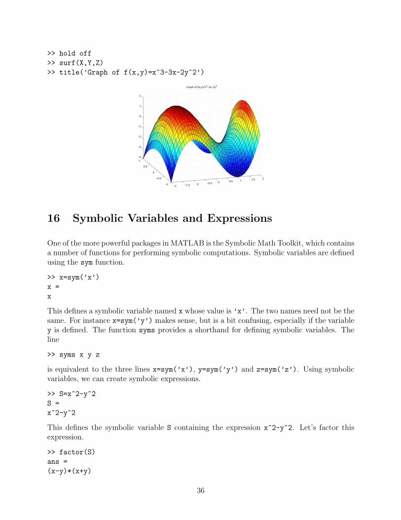
>> hold off

>> surf(X,Y,Z)

>> title(’Graph of f(x,y)=x^3-3x-2y^2’)

−2 −1.5 −1 −0.5 0 0.5 1 1.5 2

−1

−0.5

0

0.5

1−4

−3

−2

−1

0

1

2

Graph of f(x,y)=x3−3x−2y2

16 Symbolic Variables and Expressions

One of the more powerful packages in MATLAB is the Symbolic Math Toolkit, which containsa number of functions for performing symbolic computations. Symbolic variables are definedusing the sym function.

>> x=sym(’x’)

x =

x

This defines a symbolic variable named x whose value is ’x’. The two names need not be thesame. For instance x=sym(’y’) makes sense, but is a bit confusing, especially if the variabley is defined. The function syms provides a shorthand for defining symbolic variables. Theline

>> syms x y z

is equivalent to the three lines x=sym(’x’), y=sym(’y’) and z=sym(’z’). Using symbolicvariables, we can create symbolic expressions.

>> S=x^2-y^2

S =

x^2-y^2

This defines the symbolic variable S containing the expression x^2-y^2. Let’s factor thisexpression.

>> factor(S)

ans =

(x-y)*(x+y)

36

Next let’s cube S and expand the result.

>> S^3

ans =

(x^2-y^2)^3

>> expand(ans)

ans =

x^6-3*x^4*y^2+3*x^2*y^4-y^6

The simplify function is quite useful in dealing with symbolic expressions.

>> S=(x^3-4*x)/(x^2+2*x)

S =

(x^3-4*x)/(x^2+2*x)

>> simplify(S)

ans =

x-2

Symbolic expressions may also be vectors and matrices.

>> syms a b

>> A=[cos(a) -sin(a); sin(a) cos(a)]

A =

[ cos(a), -sin(a)]

[ sin(a), cos(a)]

This is the matrix for counterclockwise rotation through angle a. Let’s multiply this by thematrix for rotation through angle b.

>> B=[cos(b) -sin(b); sin(b) cos(b)]

B =

[ cos(b), -sin(b)]

[ sin(b), cos(b)]

>> C=A*B

C =

[ cos(a)*cos(b)-sin(a)*sin(b), -cos(a)*sin(b)-sin(a)*cos(b)]

[ sin(a)*cos(b)+cos(a)*sin(b), cos(a)*cos(b)-sin(a)*sin(b)]

This ought to be the matrix for rotation through angle a+b (Why?).

>> simplify(C)

ans =

[ cos(a)*cos(b)-sin(a)*sin(b), -cos(a)*sin(b)-sin(a)*cos(b)]

[ sin(a)*cos(b)+cos(a)*sin(b), cos(a)*cos(b)-sin(a)*sin(b)]

Hmm, simplify did not do anything. Another option is to use simple, which looks for theshortest equivalent expression.

37

>> D=simple(C)

D =

[ cos(a+b), -sin(a+b)]

[ sin(a+b), cos(a+b)]

As expected, this is the matrix for the rotation through angle a+b.It is tempting to think of symbolic expressions as functions of the symbolic variables they

contain. They are not. Suppose we want to enter f(x, y) = (4x2 − 1)e−x2−y2as a symbolic

expression and compute f(1, 2).

>> syms x y

>> f=(4*x^2-1)*exp(-x^2-y^2)

f =

(4*x^2-1)*exp(-x^2-y^2)

>> f(1,2)

??? Index exceeds matrix dimensions.

Since f is not a function, but a variable, MATLAB reads f(1,2) as the entry in row 1,column 2 of f. But f only has one entry, the expression (4*x^2-1)*exp(-x^2-y^2). Toevaluate a symbolic expression we need to substitute values for its symbolic variables. Thisis done using the subs function.

>> subs(f,{x,y},{1,2})

ans =

0.0202

It is not necessary to substitute for all variables in a symbolic expression.

>> subs(f,x,3)

ans =

35*exp(-9-y^2)

The substituted values may also be symbolic expressions.

>> syms u v

>> subs(f,{x,y},{u+v,u-v})

ans =

(4*(u+v)^2-1)*exp(-(u+v)^2-(u-v)^2)

The subs command thus provides a method of forming composite functions.We remark here that there is a way to define functions in MATLAB that behave in

the usual manner. This is done using the inline command. For instance, the functiong(x, y) = x2 − 3xy + 2 is defined as follows.

>> g=inline(’x^2-3*x*y+2’)

g =

Inline function:

g(x,y) = x^2-3*x*y+2

38

Now we can evaluate g(2, 3) in the usual way.

g(2,3)

ans =

-12

The disadvantage of inline functions is that they cannot be manipulated symbolically.

>> g^2

??? Error using ==> ^

Function ’^’ not defined for variables of class ’inline’.

17 Solving Algebraic Equations

The solve command is used to find solutions of equations involving symbolic expressions.

>> solve(’sin(x)+x=5’)

ans =

5.6175550052726989176213921571114

In expressions with more than one variable, we can solve for one or more of the variables interms of the others. Here we find the roots of the quadratic ax2 + bx+ c in x in terms of a, band c. By default solve sets the given expression equal to zero if an equation is not given.

>> solve(’a*x^2+b*x+c’,’x’)

ans =

[ 1/2/a*(-b+(b^2-4*a*c)^(1/2))]

[ 1/2/a*(-b-(b^2-4*a*c)^(1/2))]

Systems of equations can also be handled by solve.

>> S=solve(’x+y+z=1’,’x+2*y-z=3’)

S =

x: [1x1 sym]

y: [1x1 sym]

The variable S contains the solution, which consists of x and y in terms of z.

>> S.x

ans =

-3*z-1

>> S.y

ans =

2*z+2

Now let’s find the points of intersection of the circles x2 + y2 = 4 and (x−1)2 +(y−1)2 = 1.

39

>> S=solve(’x^2+y^2=4’,’(x-1)^2+(y-1)^2=1’)

S =

x: [2x1 sym]

y: [2x1 sym]

>> [S.x S.y]

ans =

[ 5/4-1/4*7^(1/2), 5/4+1/4*7^(1/2)]

[ 5/4+1/4*7^(1/2), 5/4-1/4*7^(1/2)]

The points of intersection are therefore ((5−√7)/4, (5+√

7)/4) and ((5+√

7)/4, (5−√7)/4).

18 Derivatives

Differentiation of a symbolic expression is performed by means of the function diff. Forinstance, let’s find the derivative of f(x) = sin(ex).

>> syms x

>> f=sin(exp(x))

f =

sin(exp(x))

>> diff(f)

ans =

cos(exp(x))*exp(x)

The nth derivative of f is diff(f,n).

>> diff(f,2)

ans =

-sin(exp(x))*exp(x)^2+cos(exp(x))*exp(x)

To compute the partial derivative of an expression with respect to some variable we specifythat variable as an additional argument in diff. Let f(x, y) = x3y4 + y sin x.

>> syms x y

>> f=x^3*y^4+y*sin(x)

f =

x^3*y^4+y*sin(x)

First we compute ∂f/∂x.

>> diff(f,x)

ans =

3*x^2*y^4+y*cos(x)

Next we compute ∂f/∂y.

40

>> diff(f,y)

ans =

4*x^3*y^3+sin(x)

Finally we compute ∂3f/∂x3.

>> diff(f,x,3)

ans =

6*y^4-y*cos(x)

The Jacobian matrix of a function f : Rn → Rm can be found directly using the jacobianfunction. For example, let f : R2 → R3 be defined by f(x, y) = (sin(xy), x2 + y2, 3x− 2y).

>> f=[sin(x*y); x^2+y^2; 3*x-2*y]

f =

[ sin(y*x)]

[ x^2+y^2]

[ 3*x-2*y]

>> Jf=jacobian(f)

Jf =

[ cos(y*x)*y, cos(y*x)*x]

[ 2*x, 2*y]

[ 3, -2]

In the case of a linear transformation, the Jacobian is quite simple.

>> A=[11 -3 14 7;5 7 9 2;8 12 -6 3]

A =

11 -3 14 7

5 7 9 2

8 12 -6 3

>> syms x1 x2 x3 x4

>> x=[x1;x2;x3;x4]

x =

[ x1]

[ x2]

[ x3]

[ x4]

>> T=A*x

T =

[ 11*x1-3*x2+14*x3+7*x4]

[ 5*x1+7*x2+9*x3+2*x4]

[ 8*x1+12*x2-6*x3+3*x4]

Now let’s find the Jacobian of T.

>> JT=jacobian(T)

JT =

41

[ 11, -3, 14, 7]

[ 5, 7, 9, 2]

[ 8, 12, -6, 3]

The Jacobian of T is precisely A.Next suppose f : Rn → R is a scalar valued function. Then its Jacobian is just its

gradient. (Well, almost. Strictly speaking, they are the transpose of one another since theJacobian is a row vector and the gradient is a column vector.) For example, let f(x, y) =(4x2 − 1)e−x2−y2

.

>> syms x y real

>> f=(4*x^2-1)*exp(-x^2-y^2)

f =

(4*x^2-1)*exp(-x^2-y^2)

>> gradf=jacobian(f)

gradf =

[ 8*x*exp(-x^2-y^2)-2*(4*x^2-1)*x*exp(-x^2-y^2), -2*(4*x^2-1)*y*exp(-x^2-y^2)]

Next we use solve to find the critical points of f .

>> S=solve(gradf(1),gradf(2));

>> [S.x S.y]

ans =

[ 0, 0]

[ 1/2*5^(1/2), 0]

[ -1/2*5^(1/2), 0]

Thus the critical points are (0, 0), (√

5/2, 0) and (−√5/2, 0).The Hessian of a scalar valued function f : Rn → R is the n× n matrix of second order

partial derivatives of f . In MATLAB we can obtain the Hessian of f by computing theJacobian of the Jacobian of f . Consider once again the function f(x, y) = (4x2 − 1)e−x2−y2

.

>> syms x y real

>> f=(4*x^2-1)*exp(-x^2-y^2)

f =

(4*x^2-1)*exp(-x^2-y^2)

>> Hf=jacobian(jacobian(f));

>> Hf=simple(Hf)

Hf =

[2*exp(-x^2-y^2)*(2*x+1)*(2*x-1)*(2*x^2-5), 4*x*y*exp(-x^2-y^2)*(-5+4*x^2)]

[4*x*y*exp(-x^2-y^2)*(-5+4*x^2), 2*exp(-x^2-y^2)*(-1+2*y^2)*(2*x+1)*(2*x-1)]

We can now use the Second Derivative Test to determine the type of each critical point of ffound above.

42

>> subs(Hf,{x,y},{0,0})

ans =

10 0

0 2

>> subs(Hf,{x,y},{1/2*5^(1/2),0})

ans =

-5.7301 0

0 -2.2920

>> subs(Hf,{x,y},{-1/2*5^(1/2),0})

ans =

-5.7301 0

0 -2.2920

Thus f has a local minimum at (0, 0) and local maxima at the other two critical points.Evaluating f at the critical points gives the maximum and minimum values of f .

>> subs(f,{x,y},{0,0})

ans =

-1

>> subs(f,{x,y},{’1/2*5^(1/2)’,0})

ans =

4*exp(-5/4)

>> subs(f,{x,y},{’-1/2*5^(1/2)’,0})

ans =

4*exp(-5/4)

Thus the minimum value of f is f(0, 0) = −1 and the maximum value is f(√

5/2, 0) =f(−√5/2, 0) = 4e−5/4. The graph of f is shown below.

−2 −1.5 −1 −0.5 0 0.5 1 1.5 2

−2

−1

0

1

2−1

−0.5

0

0.5

1

1.5

Graph of f(x,y)=(4x2−1)e−x2−y

2

As our final example, we solve a Lagrange multiplier problem. For f(x, y) = xy(1 + y)let’s find the maximum and minimum of f on the unit circle x2 + y2 = 1. First we enter thefunction f and the constraint function g(x, y) = x2 + y2 − 1.

>> syms x y mu

>> f=x*y*(1+y)

43

f =

x*y*(1+y)

>> g=x^2+y^2-1

g =

x^2+y^2-1

Next we solve the Lagrange multiplier equations ∇f(x, y) − µ∇g(x, y) = 0 and constraintequation g(x, y) = 0 for x, y and µ.

>> L=jacobian(f)-mu*jacobian(g)

L =

[ y*(1+y)-2*mu*x, x*(1+y)+x*y-2*mu*y]

>> S=solve(L(1),L(2),g)

S =

mu: [5x1 sym]

x: [5x1 sym]

y: [5x1 sym]

Next let’s view the critical points found. We can ignore µ now.

>> [S.x S.y]

ans =

[ 1/6*(22-2*13^(1/2))^(1/2), 1/6+1/6*13^(1/2)]

[ -1/6*(22-2*13^(1/2))^(1/2), 1/6+1/6*13^(1/2)]

[ 1/6*(22+2*13^(1/2))^(1/2), 1/6-1/6*13^(1/2)]

[ -1/6*(22+2*13^(1/2))^(1/2), 1/6-1/6*13^(1/2)]

[ 0, -1]

Next we need to evaluate f at each of these points.

>> values=simple(subs(f,{x,y},{S.x,S.y}))

values =

[ 1/216*(22-2*13^(1/2))^(1/2)*(1+13^(1/2))*(7+13^(1/2))]

[ -1/216*(22-2*13^(1/2))^(1/2)*(1+13^(1/2))*(7+13^(1/2))]

[ 1/216*(22+2*13^(1/2))^(1/2)*(-1+13^(1/2))*(-7+13^(1/2))]

[ -1/216*(22+2*13^(1/2))^(1/2)*(-1+13^(1/2))*(-7+13^(1/2))]

[ 0]

Finally we convert these into decimal expressions to identify the maximum and minimum.This is done using the double command.

>> double(values)

ans =

0.8696

-0.8696

-0.2213

0.2213

0

Thus the maximum of f is about 0.8696 and the minimum is about −0.8696.

44

19 M-Files

MATLAB can also be used as a programming language. MATLAB programs are calledM-files, and are saved with the extension .m. There are two types of M-files, scripts andfunctions. We will only discuss scripts here. A MATLAB script is a program which simplyexecutes lines of MATLAB code. Scripts are particularly useful for tasks that require severallines of code. Rather than retyping every line when we want to make a small change, wecan simply change one line of the script. A script consists of a plain text file with a list ofMATLAB commands that we wish to execute. Here is an example of a script.

% <-- The % is for comments.

% MATLAB ignores everything following it on the same line.

% test.m

A=[1 2; 3 4]

B=[5 6; 7 8]

A+B

After creating a file containing the text above, we save it with the filename test.m. InMATLAB we access this file by typing test. Note that, in order for this to work we must besure that the current directory in MATLAB contains the file. The Unix commands ls (listcontents of current directory), cd (change directory) and pwd (list name of current directory)all work within MATLAB.

>> test

A =

1 2

3 4

B =

5 6

7 8

ans =

6 8

10 12

MATLAB executes the commands in the M-file in order, as if we had typed them withinMATLAB. We can also do loops within a script.

% sumsquares.m

% sums the first n squares up to n=10

s=0;

for n=1:10

s=s+n^2

end

45

Here is what this looks like in MATLAB.

>> sumsquares

s =

1

s =

5

s =

14

s =

30

s =

55

s =

91

s =

140

s =

204

s =

285

s =

385

Here’s one last example to try. It shows an animation of the curve r(t) = (2t cos t/(t +1), 2t sin t/(t+1)) being plotted. See the Plotting Curves section for details on the commandsused.

% curve.m

% Shows animation of a parametric curve being plotted.

hold on

for T=0:.1:4*pi

t=[T T+.1];

plot(2*t.*cos(t)./(t+1),2*t.*sin(t)./(t+1))

axis equal

axis([-2 2 -2 2])

axis off

pause(.01)

end

46