MATWIN: A JAVA TOOL FOR EXPERIMENTING AND

COMPUTING IN DYNAMICAL SYSTEMS

____________________

A Project

Presented to the

Faculty of

California State University,

San Bernardino

____________________

In Partial Fulfillment

Of the Requirements for the Degree

Master of Science

in

Computer Science

____________________

by

Ehab Aziz Rezk

July 2007

ii

MATWIN: A JAVA TOOL FOR EXPERIMENTING AND

COMPUTING IN DYNAMICAL SYSTEMS

____________________

A Project

Presented to the

Faculty of

California State University,

San Bernardino

____________________

by

Ehab Aziz Rezk

August 2007

Approved by:

Dr. Keith Schubert, Chair, Computer Science Date

Dr. Ernesto Gomez

Dr. Richard J. Botting

iii

ABSTRACT

The dynamics of any situation refers to how the

situation changes over the course of time. A basic

observation of dynamical systems is how extraordinarily

complicated the motions of a system can be, even when the

underlying rules are extremely simple. One of the main

approaches to dynamical systems is Differential

equations. Given any initial state, a differential

equation, or a system of differential equations are used

to describe the forces, or directions in which a system

is being pushed. In many cases where exact solutions for

differential equations are hard to find, approximate

solutions can be calculated using numerical solution

methods such as Euler and Runge Kutta. Here, I present

MATWIN, a toolkit for Windows computers, consisting of

four graphics programs. It supports mathematical

computation and experimentation in dynamical systems.

This software was developed for a college level courses

that teach dynamical systems or differential equations.

Also, because one of the programs included in this

software deals with basic calculus topics such as drawing

curves of functions, drawing tangents at desired points,

finding roots, area under curves, maxima and minima, it

iv

can be of great help to high school calculus students

too.

v

ACKNOWLEDGMENTS

As I present my project, I would like to express my

thanks to Dr. K. Schubert, my project supervisor, for

proposing the idea of MATWIN, and for providing me with

his knowledge and support. Also, I would like to thank

Dr. R. Botting for being the first to introduce me to the

programming world when I first started my program with

C++ class. Also, special thanks to Dr. Gomez for giving

me his great comments that made my project better. As the

happiness fills my soul for completing this project and

my degree requirements as well, a special word of thanks

I would like to say to the Faculty and Staff of Computer

Science department at California State University, San

Bernardino, for providing this master’s program in

Computer Science, and for giving me this great

opportunity to join and graduate from it.

Also I would like to express my deep gratitude to my

dear wife, Sherein, my kids, Karen and Martin, my father,

William, mother, Aida, and my beloved brothers, Mina,

Sameh, and Bishoy for supporting and encouraging me at

every hard time.

vi

TABLE OF CONTENTS

ABSTRACT . . . . . . . . . . . . . . . . . . . . . . iii

ACKNOWLEDGEMENTS . . . . . . . . . . . . . . . . . . v

LIST OF TABLES . . . . . . . . . . . . . . . . . . . ix

LIST OF FIGURES . . . . . . . . . . . . . . . . . . x

CHAPTER ONE: INTRODUCTION . . . . . . . . . . . . . 1

Scope . . . . . . . . . . . . . . . . . . . . . 3

Purpose . . . . . . . . . . . . . . . . . . . . 4

Project Products . . . . . . . . . . . . . . . 4

Source Code and Compiled Classes . . . . . 4

User Guide . . . . . . . . . . . . . . . . 5

Project presentation . . . . . . . . . . . 5

CHAPTER TWO: MATHEMATICAL APPROACH

Differential Equations . . . . . . . . . . . . . 6

Numerical Solutions . . . . . . . . . . . . . . 7

Simpson Rule . . . . . . . . . . . . . . . 7

Newton Method . . . . . . . . . . . . . . . 8

Bisection Method . . . . . . . . . . . . . 9

Runge Kutta Algorithm . . . . . . . . . . . 10

Slope Fields . . . . . . . . . . . . . . . . . 11

MATWIN Mathematical Features . . . . . . . . . . 12

The One-Dimensional Case . . . . . . . . . 12

Raising The Number of Dimensions . . . 17

vii

The Two-Dimensional Case . . . . . . . . . 18

Linear Equations With Constant Variables . . . . . . . 21

Nonlinear Equations . . . . . . . . . 24

The Three-Dimensional Case . . . . . . . 28

CHAPTER THREE: PROJECT DEVELOPMENT AND DESIGN

Development Tools . . . . . . . . . . . . . . . 31

Running Requirements . . . . . . . . . . . . . . 31

Project Design . . . . . . . . . . . . . . . . . 31

Quick Synopsis Of The Program . . . . . . . . . 34

The Analyzer . . . . . . . . . . . . . . . 34

DiffEq . . . . . . . . . . . . . . . . . . 35

DiffEq, Phase Plane . . . . . . . . . . . . 35

DiffEq, 3Dview . . . . . . . . . . . . . . 36

CHAPTER FOUR: USER MANUAL

Introduction . . . . . . . . . . . . . . . . . 37

The Analyzer (The Main Screen) . . . . . . . . . 38

Inserting Expressions . . . . . . . . . . 40

Using The Calculator Feature . . . . . . . 43

Plotting Functions . . . . . . . . . . . . 43

Changing Graph Scales . . . . . . . . . . . 46

Drawing Tangents And Derivatives . . . . . 47

Finding Roots, Maxima And Minima Coordinates . . . . . . 49

viii

Difinite Integrals . . . . . . . . . . . . 51

Saving And Printing . . . . . . . . . . . . 52

Launching Other Applications . . . . . . . 54

DiffEq And DiffEq, Phase Plane . . . . . . . . . 54

Displaying The Slope Fields And Solutions . . . . . . . . 56

Saving And Printing . . . . . . . . . . . 58

DiffEq, 3Dview . . . . . . . . . . . . . . . . . 59

Rotation, Translation, And Zooming . . . . 62

Saving and Printing . . . . . . . . . . . 64

CHAPTER FIVE: CONCLUSION AND FUTUR EXTENSIONS

Summary . . . . . . . . . . . . . . . . . . . 65

Program Evaluation . . . . . . . . . . . . . . . 66

Future Extensions . . . . . . . . . . . . . . . 67

APPENDIX A: SAMPLE CODE . . . . . . . . . . . . . . 69

REFERENCES . . . . . . . . . . . . . . . . . . . . . 136

ix

LIST OF TABLES

Table 4.1. Syntax Accepted By MATWIN . . . . . . . . 42

x

LIST OF FIGURES

Figure 2.1. Simpson Method . . . . . . . . . . . . . 8

Figure 2.2. Newton Method . . . . . . . . . . . . . 9

Figure 2.3. Bisection Method . . . . . . . . . . . 10

Figure 2.4. Slope Field Diagram . . . . . . . . . 12

Figure 2.5. Slope Field for xydxdy 2/ . . . . . . 13

Figure 2.6. Single Solution Through 0)0( x . . . . 15

Figure 2.7. Multiple Solutions. . . . . . . . . . . 16

Figure 2.8. Multiple Solutions Of xdtxd 22 / . . . 19

Figure 2.9. Equilibria Types . . . . . . . . . . . 21

Figure 2.10. Solutions Of ydtdx / & yxdtdy 21/ . . 23

Figure 2.11. Some Possible Degenerate Equilibria . . 24

Figure 2.12. Nonlinear System Phase Plane . . . . . . 25

Figure 2.13. Limit Cycle . . . . . . . . . . . . . . 25

Figure 2.14. Phase Plane Of Nonlinear System . . . . 27

Figure 2.15. Phase Plane Of Linear System . . . . . . 27

Figure 2.16. 3D-View For ydtdx / , xdxdy / , and 1/ dtdz . . . . . 29

Figure 2.17. Rotated 3D-View For ydtdx / , xdxdy / ,

and 1/ dtdz for 0,0,1 ooo zyx . . . . . 30

Figure 3.1. The Basic MATWIN Architicture . . . . . 32

Figure 4.1. The Main Screen . . . . . . . . . . . . 38

xi

Figure 4.2. Expression Fields . . . . . . . . . . . 41

Figure 4.3. The Calculator Feature . . . . . . . . 43

Figure 4.4.a. Pressing “Draw Y1” Button . . . . . . . 44

Figure 4.4.b. Pressing “Draw Y2” Button . . . . . . . 45

Figure 4.4.c. Pressing Both Buttons . . . . . . . . . 45

Figure 4.5. Changing The Scales And Divisions Along Axes . . . . 47

Figure 4.6. Derivatives and Tangents . . . . . . . 49

Figure 4.7. Calculated Roots And Max_Min Values . . 50

Figure 4.8. Finding The Definite Integral . . . . . 52

Figure 4.9. Print Dialog Box . . . . . . . . . . . 53

Figure 4.10. DiffEq Screen . . . . . . . . . . . . . 55

Figure 4.11. DiffEq Slope Field and Solutions . . . 57

Figure 4.12. The Phase Plane Solution Trajectories . . . . . . 58

Figure 4.13. The view Of The Solution To 3 Differential Equations . . . . . . 60

Figure 4.14. 3D View With

Rotation Arround X And A Axes . . . . . 62

Figure 4.15. Mouse Rotation, Translation, and Zooming . . . . . . . 63

1

CHAPTER ONE

INTRODUCTION

The dynamics of any situation refers to how the

situation changes over the course of time. A dynamical

system is a mathematical model of a system often in a

physical setting, which specifies the rules for how the

setting changes or evolves from one moment of time to the

next. The theory of differential systems is the tool with

which scientists make mathematical models to represent

the real systems. One basic goal of the mathematical

theory of dynamical systems is to determine or

characterize the long-term behavior of the system.

A basic observation of dynamical systems, largely

due to the advent of computers and computer graphics, is

how extraordinarily complicated the motions of a system

can be, even when the underlying rules are extremely

simple. An example for this is the Newton’s description

of the motion of bodies under gravity. The forces are

extremely simple: bodies attract to each other by a force

proportional to the product of their masses and inversely

proportional to the square of the distances separating

them. Yet the motions caused by these forces are

2

extremely complex, resulting, for instance, in the

braided rings of Saturn.

One of the main approaches to dynamical systems is

Differential equations. Given any initial state, a

differential equation, or a system of differential

quations are used to describe the forces, or directions

in which a system is being pushed. Some of these

differntial equations are easy to solve using integration

methods to get exact solutions, while in some other

cases, it is hard or even impossible to find exact

solutions to other system of differential equations. In

such these cases where exact solutions are hard to find,

approximate solutions can be calculated using numerical

solution methods such as Euler and Runge Kutta. These

numerical methods require a huge amount of calculations

that need to be repeated over and over for huge number of

times, which is a waste of time plus the fact that these

repeated calculations can lead to huge mistakes in the

final values calculated.

In the 1940s an entirely new tool of analysis also

came on the scene-the digital computer. In addition to

its obvious brute-force capabilities of grinding out

nummerical solutions of differential equations, it

3

presents a flexible, interactive tool for the purpose of

discoveries. This interplay between computations and

analysis has proved to be of great importance, and

represents one of the major methods of uncovering dynamic

properties. Indeed, the area of computer science has

rapidly progressed to a state in which it can now make

fundamental contributions to our knowledge, rather than

acting only as the servant of other methods of analysis.

Here, I present MATWIN, a toolkit for Windows

computers, consisting of four graphics programs. It

supports mathematical computation and experimentation in

dynamical systems. This software was developed for a

college level courses that teach dynamical systems or

differential equations. Also, because one of the programs

included in this software deals with basic calculus

topics such as drawing curves of functions, drawing

tangents at desired points, finding roots, area under

curves, maxima and minima, it can be of great help to

high school calculus students too.

Scope

MATWIN is intended to be for the college level

students who study dynamical systems or differential

4

equations. Also it can be of great help to high school

calculus students.

Purpose

The purpose of this project is to implement an

integrated piece of software consisting of a number of

graphics programs that support mathematical computation

and experimentation in dynamical systems. These graphics

programs should be able to draw the solutions to the

given differential equations (automatically, using

standard numerical methods) without dealing with the

complications of the analytic techniques from the user

side.

Project Products

Upon project completion, the following products will

be delivered.

Source Code and Compiled Classes:

The project consists of four applets. The source

files contain the implementation of all applets,

along with the parser, the methods for finding the

roots, derivatives, maxima and minima, and finding

the solutions to the given differential equations.

5

Also they contain all the comments within the source

code for relevant statements and methods.

User Guide:

The user guide contains documentation of this

project’s products. Detailed instructions are

provided for:

o Using the main applet (Analyzer).

o Using the DiffEq. applet.

o Using the Phase Plane applet.

o Using the 3Dview applet.

The user guide includes a detailed description

covering all the features of the program. This guide

includes also a number of examples of systems of

differential equations along with their graph

solutions for evaluation purposes.

Project Presentation:

A presentation will be given to the public, wherein

the overview of the system will be introduced.

6

CHAPTER TWO

MATHEMATICAL APPROACH

Differential Equations

A differential equation is an equation involving an

unknown function and its derivatives. The equation can

contain only one variable and be called Ordinary, or can

contain more than one variable and need to be solved

along with other equations. Using analytical techniques,

as direct integration and separating variables, can solve

a wide range of differential equation systems.

Unfortunately the equations resulting from modeling real

world don’t usually fall into that category of

differential equations that can be solved analytically.

In such those cases, where the exact solution can’t be

found by analytical methods, some well known algorithms

known as numerical methods can find these solutions with

a satisfied degree of accuracy.

Using MATWIN enables dealing with equations whether

or not they can be solved analytically. if the equations

can be stated as functions in one of the following forms:

7

One-dimensional two-dimensional three-dimensional

),( xtfdt

dx

),(

),(

yxgdt

dx

yxfdt

dx

),,(

),,(

),,(

zyxhdt

dz

zyxgdt

dy

zyxfdt

dx

then they can be entered in MATWIN program. Higher

order equation involving second and third derivatives can

be rewritten to fit the above formats. Once the equations

are entered, MATWIN can draw the solutions

(automatically, using standard numerical methods, to be

discussed later) without any further user calculations.

Numerical Solutions

Four numerical solutions were used in MATWIN:

Simpson rule

Simpson rule, figure 2.1, is a method for finding

the definite integral, within a certain range, to a

function f(x) by dividing the area under the curve of

f(x) into a number of trapeziums and then finding the

total area by getting the sum of these areas.

8

Figure 2.1. Simpson method

Newton method

Newton method, figure 2.2, is very efficient way of

finding roots of complicated functions. For any function

f(x), the algorithm starts by guessing an initial value,

xo, to be the first approximation of the root. A tangent

line to the curve f(x) at x = xo is drawn, and then a more

precise solution can be found at the intersection of this

tangent line and X-axis. The process can be repeated for

any number of times until the desired accuracy is

achieved.

9

Figure 2.2. Newton method

Bisection method

This method, figure 2.3, is used to find the roots

of a function g(z)if the graph of g(z) crosses X-axis. It

is efficient in catching the crossing points that were

not detected by Newton method. The root can be found by

choosing two points z1 and z2. if g(z1)*g(z2) = -1, then

there is a root between z1 and z2. Finding the midpoint,

zm =(z1+z2)/2, of z1 and z2 gives the first approximation

of the root. Repeating these steps for z1 and zm or zm

and z2 gives a better approximation and so on.

10

Figure 2.3. Bisection method

Runge Kutta Algorithm

The Runge-Kutta algorithm is the magic formula

behind solving differential equations numerically. It is

known to be very accurate and well behaved for a wide

range of problems.

For a single variable problem x’ = f (t, x),

If xn is the value of the variable at time tn , then xn+1

at time, tn+h is

xn+1 = xn + h⁄6 (a + 2 b + 2 c + d)

Where

a = f (tn, xn) ,

b = f (tn + h⁄2, xn + h⁄2 a),

c = f (tn + h⁄2, xn + h⁄2 b), and

11

d = f (tn + h, xn + h c).

For multi variable cases, the algorithm is still the

same, with one exception. Each variable becomes a vector.

Then

where

Slope Fields

The slope field of a differential equation dy/dt =

f(x,y) is a diagram with little line segments, drawn at

the points of some grid, with the slope as given by the

differential equation. These diagrams can be used to have

a quick idea of what the solution may look like. Figure 4

shows the slope field diagram for (a) dy/dt = x+y, and

(b) dy/dt = x2

)22(6

1 nnnnnn dcbah

xx

)(

)2

(

)2

(

)(

nnn

nnn

nnn

nn

chxfd

bh

xfc

ah

xfb

xfa

12

Figure 2.4. Slope Field diagrams

(a) dy/dt = x+y (b) dy/dt = x2

MATWIN Mathematical Features

To better understand the mathematical features of

MATWIN, let us discuss the following three cases:

The One-Dimensional case

For DiffEq equation ),( xtfdt

dx describes a slope field

in the tx-plane. For any particular point (t,x) the

equation tells exactly the slope of the solution through

that point. The program draws the slope field by

13

plotting, at the points of some grid, little line

segments with the slope as given by the differential

equation.

Figure 2.5. Slope Field for xydxdy 2/

A solution x(t)of the differential equation is a

function of t, which can be most easily imagined as a

graph whose slope at every point(t,x)is f(t,x).

If a point (to,xo) is chosen by the cursor, the

program will draw an approximate solution through that

14

point. The point (to,xo) is called the initial condition

for the solution for that solution. The general idea of

the approximate solution is that the computer calculates

the slope at the initial condition point and increments

the step and then calculates the slope at the new

position; then it repeats incrementing the step and

calculation the new slope values until it reaches the

boundary of the screen. Then the program goes back to the

starting point (initial condition) and repeats the

process in the opposite direction. This is done by

decrementing time in Runge Kutta equation.

At the far right of the graph, figure 6, the slope

field changes rapidly near the solution drawn, but it has

been calculated carefully with a step size of less than

one pixel, so at every point graphed it indeed has the

proper slope, as if a slope mark were centered on that

point. The approximate solution travels “with the flow”

through the slope field.

15

Figure 2.6. Single solution through 0)0( x

An approximate solution made in this way can be as

accurate as you want. Choosing a smaller step size will

perform better id desired.

Using MATWIN you can choose any number of initial

conditions (by clicking the mouse at any desired point)

and have multiple solutions drawn together at the same

graph, figure 2.7.

16

Figure 2.7. Multiple solutions

Now, one can have a global idea on how the solutions

(at different initial points) may look like, which enable

a qualitative analysis quite unavailable from non

graphical numerical listings of individual solutions.

Furthermore, notice that the entire procedure of

drawing an approximate solution uses only the slope, as

given explicitly by the differential equation; it never

makes any reference to an explicit analytic solution. The

graphics program totally bypasses the need for such

analytic calculation.

17

For the case of the above examples, xyy 2' does

not fit any of the special solutions for analytic

solutions; moreover, it can actually be proven (with very

advanced mathematics from differential Galois theory)

that for this particular equation there is no formula for

the solutions in terms of elementary functions (the

functions we normally write, like polynomials, rational

functions, trigonometric functions, and other

transcendental functions). Nevertheless the solutions do

exist, and still can be seen graphically.

Raising the Number of dimensions

Similar pictures can be drawn for a differential

equation of higher order or with more variables. The

overriding principle for changing a higher order equation

in x into a system is to set ydtdx / . If a higher degree

is necessary, set zdtdy / and continue, Example 2.1.

18

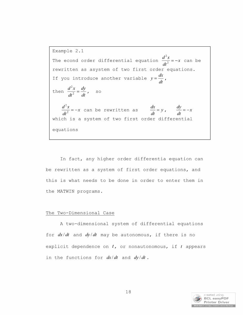
In fact, any higher order differentia equation can

be rewritten as a system of first order equations, and

this is what needs to be done in order to enter them in

the MATWIN programs.

The Two-Dimensional Case

A two-dimensional system of differential equations

for dtdx / and dtdy / may be autonomous, if there is no

explicit dependence on t, or nonautonomous, if t appears

in the functions for dtdx / and dtdy / .

Example 2.1

The econd order differential equation xdt

xd

2

2

can be

rewritten as asystem of two first order equations.

If you introduce another variable dt

dxy ,

then dt

dy

dt

xd

2

2

, so

xdt

xd

2

2

can be rewritten as ydt

dx , x

dt

dy

which is a system of two first order differential

equations

19

An autonomous system describes a vector field in the

xy-plane, the phase plane, consisting only of the

dependent variables. Through any give point ),( oo yx , the

program DiffEq, Phase Plane will draw a trajectory, which

is the xy-path determined parametrically by the solutions

)(tux and )(tvy . For any particular point ),( oo yx the

equation tells exactly the slope of the trajectory

through that point by

dtdx

dtdy

dx

dy

/

/

Figure 2.8. Multiple solutions of xdtxd 22 / .

20

Figure 2.8. shows the solution of the equation

xdtxd 22 / as equivalent to the two equations: ydtdx / &

xdtdy / .

The phase plane, however, shows how x and y

interact; it is an extremely important picture. In

particular, the phase plane phase plane gives crucial

information about the behavior of trajectories near all

possible equilibria. Also for an autonomous system of

differential equations, the trajectories normally will

not meet or cross each other (except at equilibria).

Equilibrium, or a singularity, is a point where the

derivative of each variable is zero; for the example in

figure 2.7, the equilibrium is at (0,0). Equilibrium may

be either stable or unstable, according to whether nearby

trajectories approach or leave that point. The center in

figure 7 was stable.

If a system is linear, with constant coefficients,

then a great deal is known about the behavior of the

trajectories. In fact, traditionally the only big success

at finding analytic solutions was in dealing with linear

equations with constant coefficients.

21

Nonlinear systems turn out not to be so different as

one might think, now that phase plane pictures are so

readily obtained. The phase plane allows us to see what

happens to trajectories, especially near singularities,

and to see that there the nonlinear equations behave

exactly as the linear ones. So phase analysis for linear

equations even serves for nonlinear ones.

Linear Equations With Constant Coefficients

In a two-dimensional system of differential

equations, there are essentially four types of equilbria,

named:

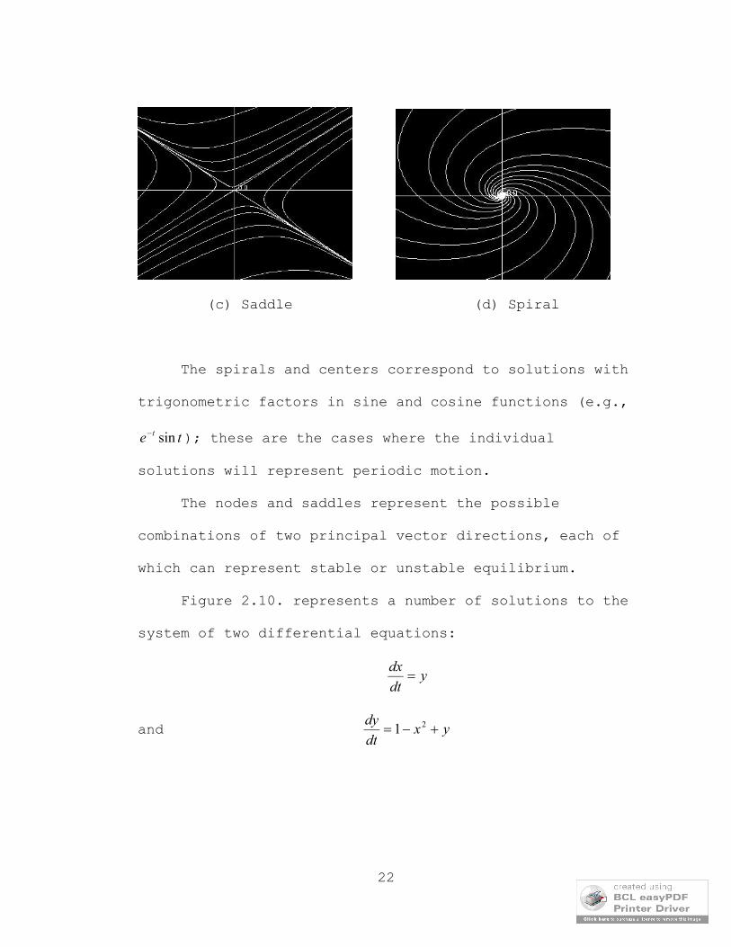
Figure 2.9. Equilibria types

(a) Center (b) Node source

Figure 2.9. continue

22

(c) Saddle (d) Spiral

The spirals and centers correspond to solutions with

trigonometric factors in sine and cosine functions (e.g.,

te t sin ); these are the cases where the individual

solutions will represent periodic motion.

The nodes and saddles represent the possible

combinations of two principal vector directions, each of

which can represent stable or unstable equilibrium.

Figure 2.10. represents a number of solutions to the

system of two differential equations:

ydt

dx

and yxdt

dy 21

23

Figure 2.10. Solutions of ydtdx / & yxdtdy 21/

The graph shows spiral singularity at (1,0) and a saddle

at (-1,0).

A linear system of two first order differential

equations (alternatively, a single second order equation)

will exhibit a single equilibrium or singularity, showing

one of six behaviors (or a degenerate case, corresponding

to double and/or zero exigent values). Some degenerate

possibilities are shown in figure 2.11.

24

Figure 2.11. Some possible degenerate equilibria.

Nonlinear Equations

A nonlinear system of two first order differential

equations can have more than one equilibrium or

singularity, and may exhibit a very complicated phase

plane. Figure 11 shows an example of the phase plane for

the system of nonlinear differential equations:

)sin( yxdt

dx , And )cos(xy

dt

dy

As can be easily seen in the diagram in figure 2.12,

the phase plane exhibits spiral, saddle, and node

singularities in different places. In addition, there is

one another phase plane behavior a nonlinear system can

exhibit, that is the limit cycle, which is shown in

figure 2.13.

25

Figure 2.12. Nonlinear System phase plane.

Figure 2.13. Limit Cycle.

The Phase Plane could show all the singularities

exhibited by the nonlinear system discussed above.

26

For a nonlinear system, a good approximation to a

solution can be made by the process of linearization,

near the singularity. The linearization formulas are not

to be discussed here, but to have a little idea on this

process, let us consider the following example.

Example 2.2. (Linearization of a system of Differential Equations)

Consider the system of nonlinear ordinary

differential equations described by

)1(' xyx , and

.)3(' xyy

Using MATWIN DiffEq, Phase Plane program we can

get graphical solutions as those of the linear

systems arround some points. See figures 2.14,

and 2.15.

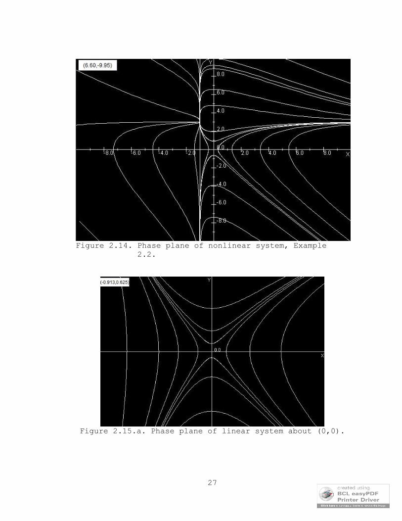
27

Figure 2.14. Phase plane of nonlinear system, Example 2.2.

Figure 2.15.a. Phase plane of linear system about (0,0).

28

Figure 2.15.b. Phase plane of linear system about (-1,3).

The Three-Dimensional Case

The program DiffEq, 3Dview is a part of MATWIN that

accepts an autonomous three-dimensional system, that is,

with no explicit dependence on t:

).,,(

),,,(

),,,(

zyxhdt

dz

zyxgdt

dy

zyxfdt

dx

In such an autonomous three-dimensional system, the

critical graph that relates x, y, and z is a three-

dimensional xyz-phase space. Figures 2.16 shows 3D-phase

29

space for a system of three differential equations

described by ydtdx / , xdxdy / , and 1/ dtdz

Figure 2.16. 3D-View for ydtdx / , xdxdy / , and 1/ dtdz

for 0,0,1 ooo zyx

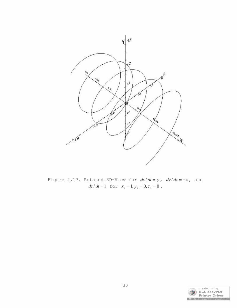
Figure 2.17 shows the same 3D-View of the last

system after applying a compound rotation of 45 degrees

around both x-axis y-axis.

30

Figure 2.17. Rotated 3D-View for ydtdx / , xdxdy / , and

1/ dtdz for 0,0,1 ooo zyx .

31

CHAPTER THREE

PROJECT DEVELOPPMENT AND DESIGN

Development Tools

MATWIN was developed using the following:

J2SE Development kit 5, update 2, (jdk-1_5_0_02-

windows-i586-p).

Java3D, (java3d-1_3_1-windows-i586-directx-sdk).

Running Requirements

In order to run MATWIN, the following requirements

are needed.

Windows 98, Windows ME, Windows 2000, Windows XP, or

Windows Vista.

Java2 SDK 1.5.0 or later from Sun Microsystems.

Java3d SDK 1_3_1-windows-i586-directx-sdk or later

from Sun.

Microsoft DirectX 8.0 or later, available from

Microsoft.

Project Design

Sixteen classes were written to develop MATWIN.

Figure 3.1 shows its basic architecture.

32

Figure 3.1. The basic MATWIN Architecture.

As can be seen above, the design of MATWIN consists

of four main parts, the fist part, the left hand side, is

the core of the project. It consists of six classes that

StringToVectorTokenizer

Equation

RootFinder

MaxMinFinder

Derivative Finder

RungeKutta

GraphArea

GraphArea2

GraphArea3

Canvas3D

OffScreenCanvas3D

DiffEqApplett

PhasePlaneApplett

3DViewApplett

MainApplett

SaveAnImage

33

perform all the basic mathematical tasks like tokenizing

and parsing inputs, finding minima and maxima, finding

roots and derivatives. Also it includes the rungeKutta

class, which uses RungeKutta algorithm to integrate a

function. These classes are called almost by every other

class in the system.

The second set of classes in the design includes

GaraphArea, GraphArea2, GraphArea3, Canvas3D, and

OffScreenCanvas3D. These classes implement the Graph

Areas of the different parts of the software. They

include methods to plot and modify the axes, methods to

draw and modify the graphs of functions, the slope

fields, and the trajectories of the solutions to the

input equations, methods to interact with the user, as in

Canvas3D, where a user can rotate, translate, and zoom

the 3D view of the solution, and methods to print and

save. These classes are called by the applet classes,

(Main Applet, DiffEqApplet, PhasePlaneApplet, and

3DviewApplett), to draw and redraw the desired views when

these applets needs to modify their contents.

The third set of classes includes Applet,

DiffEqApplet, PhasePlaneApplet, and 3DviewApplet. These

applets represent the interfaces through which the user

34

will insert expressions, input data, and draw graphs and

solutions. These Applets have methods to modify their

contents and to call other classes to perform the needed

calculations or to draw the updated view. Also they have

methods to call the print and save features in other

applets. Applet,(or main screen), is the main interface

by which all other applets can be called. It contain all

the capabilities to plot the graphs of functions, (two

functions at the same time), the tangents at desired

points, the slope graphs, to find the maxima and minima,

and the integral within a certain range.

Quick Synopsis of The Program

MATWIN consists of four graphics programs. These

programs represent the interface between the software and

the user.

The Analyzer

This part of MATWIN represents the main screen from

which all other screens can be called. For a

function y = f(x), this program draws the graph of

the function and its derivative, the tangent to the

curve at any desired point. It also finds the roots,

35

maxima and minima (by analyzing the derivative), and

numerically integrates the function within a

specific region that is determined by the user. The

Analyzer can graph two functions simultaneously

along with their derivatives and tangents. Analyzer

is a very handy tool for dealing with awkward

equations.

DiffEq

For a first order differential equation of the form

dy/dx = f(x,y), this program displays the slope

field and draws the solutions in xy-plane. The

initial condition is chosen graphically with the

cursor. The coordinates of the initial point are

displayed. The drawing of the solution proceeds

first forward in time and then backword.

DiffEq, phase Plane

For an autonomous system of differential equations

of the form

),,( yxfdt

dx ),( yxg

dt

dy

this program displays the vector field in the xy-

phase plane and draws the solution in xy-plane. As

the case with DiffEq program, the initial condition

36

is chosen graphically with the cursor and the

drawing of the solution goes forward and backwards

in time.

DiffEq, 3D Views

For autonomous systems of differential equations of

the form

),,(

),,(

),,(

zyxhdt

dz

zyxgdt

dy

zyxfdt

dx

This program draws the three-dimensional phase

space. It rotates, translates, and zoom the view

through user interaction.

37

CHAPTER FOUR

USER MANUAL

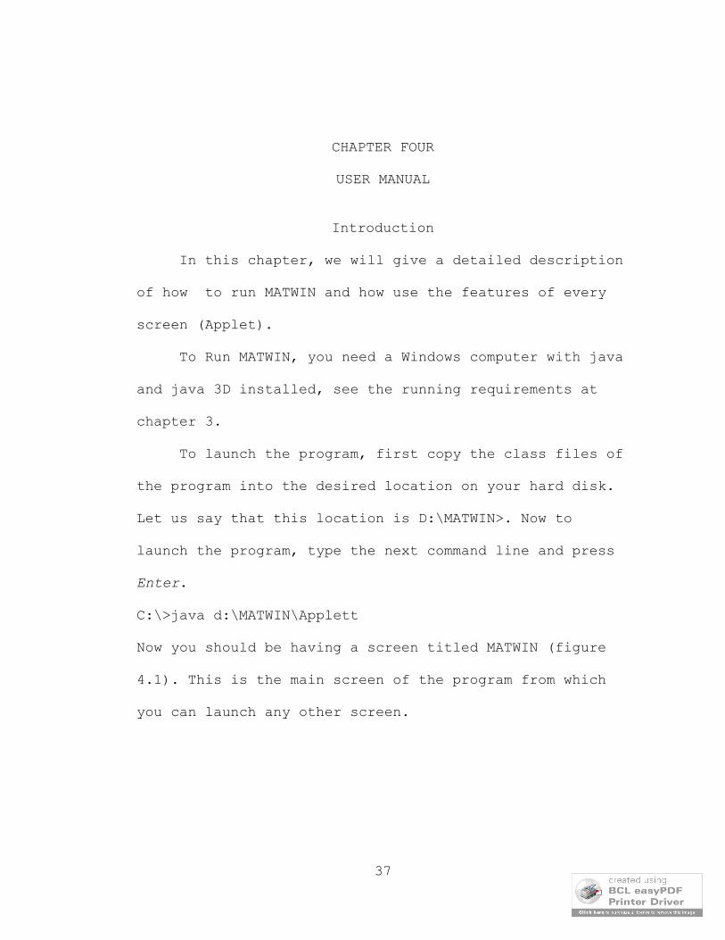
Introduction

In this chapter, we will give a detailed description

of how to run MATWIN and how use the features of every

screen (Applet).

To Run MATWIN, you need a Windows computer with java

and java 3D installed, see the running requirements at

chapter 3.

To launch the program, first copy the class files of

the program into the desired location on your hard disk.

Let us say that this location is D:\MATWIN>. Now to

launch the program, type the next command line and press

Enter.

C:\>java d:\MATWIN\Applett

Now you should be having a screen titled MATWIN (figure

4.1). This is the main screen of the program from which

you can launch any other screen.

38

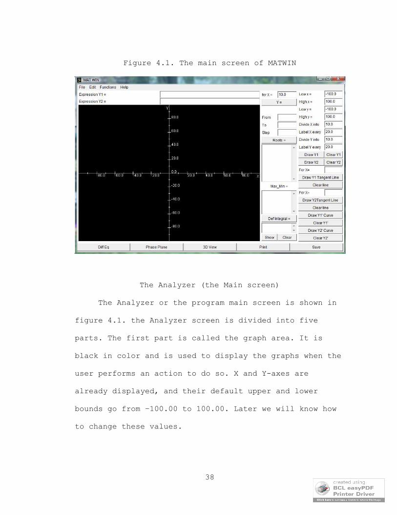
Figure 4.1. The main screen of MATWIN

The Analyzer (the Main screen)

The Analyzer or the program main screen is shown in

figure 4.1. the Analyzer screen is divided into five

parts. The first part is called the graph area. It is

black in color and is used to display the graphs when the

user performs an action to do so. X and Y-axes are

already displayed, and their default upper and lower

bounds go from –100.00 to 100.00. Later we will know how

to change these values.

39

The second part lies right above the graph area. It

consists of two expression fields labeled Expression Y1,

and Expression Y2. These are the places into which the

expressions are to be fed to the program. The Analyzer

can take two expressions at the time. One of the two

expressions will be the primary one, on which all the

calculations are performed while the other one is a

secondary one, and only some operations will be performed

on it.

The third part of the Analyzer screen is a column of

buttons, expression fields and text fields, which are

used to input data into or output data from the program.

The features of this part work only for the primary

expression (the expression on the top), You shouldn’t be

expecting to apply the features of this part to the

secondary expression (the lower one). These features

include a calculator that can evaluate the primary

expression for a given value of x, a feature to find the

roots, maxima and minima, definite integral of the

primary expression. Also you can show the area defined by

the definite integral graphically.

The column on the right side of the Analyzer

represents the fourth part of the screen. It consists of

40

a number of buttons, data fields, and text areas. Some of

these features can apply to the primary expression while

the rest apply for the secondary one. It includes

capabilities that can draw a function (expression) and

its derivative, draw the tangent to a function at any

desired point on the curve of the expression. You can

undo any step at any time by pressing the appropriate

clear button, as we will see later. Also this part

contains some fields that can be used to input the

desired lower and upper values of x and y-axes. The

boundary values of the axes can be changed at any time by

replacing the old value with the new one.

The last part of the analyzer screen is the row of

buttons located at the bottom of the screen. It contains

buttons for saving or printing the graph on the graph

are, and buttons for launching the rest of the screens,

DiffEq, DiffEq, Phase Plane, and DiffEq, 3Dview.

Inserting Expressions

Two expression can be inserted the expression field

on the top of the graph area at any time (see figure

4.2). These are the only places to insert your functions

(expressions). These expression fields accept only

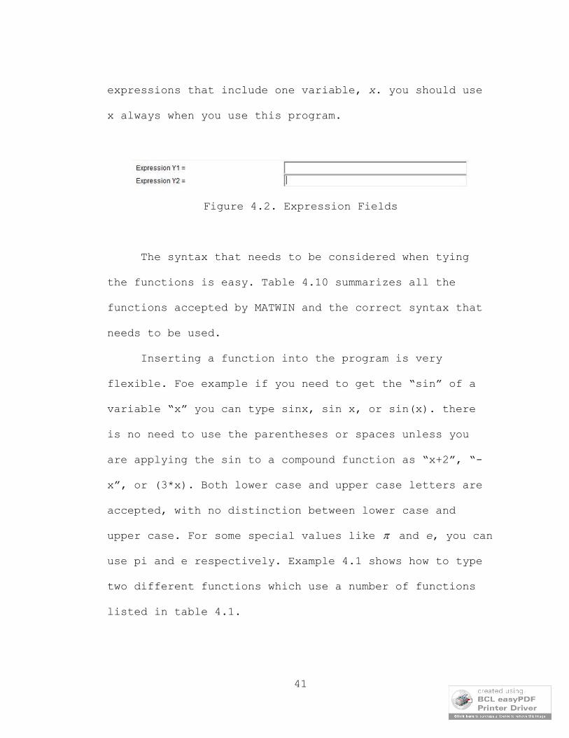
41

expressions that include one variable, x. you should use

x always when you use this program.

Figure 4.2. Expression Fields

The syntax that needs to be considered when tying

the functions is easy. Table 4.10 summarizes all the

functions accepted by MATWIN and the correct syntax that

needs to be used.

Inserting a function into the program is very

flexible. Foe example if you need to get the “sin” of a

variable “x” you can type sinx, sin x, or sin(x). there

is no need to use the parentheses or spaces unless you

are applying the sin to a compound function as “x+2”, “-

x”, or (3*x). Both lower case and upper case letters are

accepted, with no distinction between lower case and

upper case. For some special values like and e, you can

use pi and e respectively. Example 4.1 shows how to type

two different functions which use a number of functions

listed in table 4.1.

42

Function Syntax examples

Signed variable x, X, -x, pi, e, -pi, -e,..

Addition & Subtraction x+2, 3-x, -x-1, -(x+0.5),..

Multiplication & Division 2*x, x/2, (x+3)/(-4*x)

Raising to a power x^2, x^(-1.5), (-x)^(x/2.2),..

Square Root sqrt(x) for 0x x , ..

Logarithmic functions)ln(,ln xx for elog where 0x

)log(,log xx for 10log where 0x

Exponential functions exp x, exp(x), exp(x/2),..

Trigonometric functionssinx, cos(-x), atan(x),.. where x is in radians

Table 4.1. Syntax accepted by MATWIN

Note that, a numeral ‘0’ (zero) is different from an

‘O’ (oh), and a ‘1’ (one) is different from an ‘l’

Example 4.1.

(a) the expression 22 2sin xexx

is be typed sinx+e^(x/2)+(2*pi*x^2) in MATWIN.

(b) The expression )2/3/()2.2sin( xxx is typedSqrt(x+sin(-2.2*x))/((3*x)/2) into MATWIN.

43

(lower-case ‘L’). they look similar, but using the wrong

one will cause the computer to give an error message.

Using The Calculator feature

The Analyzer includes a very handy calculator

feature. It is very easy to use. Once the there is an

expression in the expression field Y1, you can calculate

the value of the expression for any desired value of x.

to calculate the value of the expression x for 25.2x ,

type the expression sqrtx in the Y1-expression field and

2.25 in the space labeled “for x =” and press the button

“Y =”.

The answer is 1.5 as shown in figure 4.3.

Figure 4.3. The Calculator Feature

The x-value and the calculated values will remain

unchanged until the user changes them.

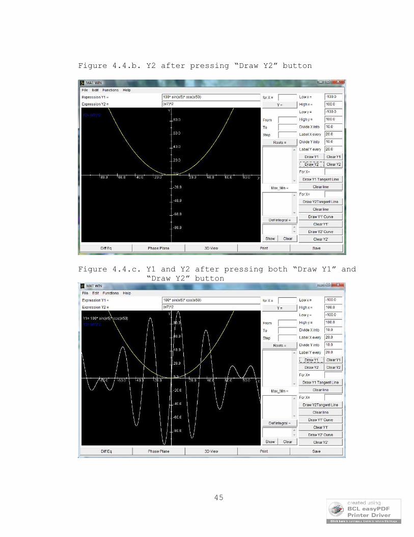
Plotting Functions

To draw a function on the graph area, you need to

insert at least one function into the expression fields

44

Y1 or Y2 or both, then press the Draw Y1, or Draw Y2, or

both. the graph area will display the curves and their

expressions, see figure 4.4.

Figure 4.4.a. The graph of Y1 after pressing “Draw Y1” button

45

Figure 4.4.b. Y2 after pressing “Draw Y2” button

Figure 4.4.c. Y1 and Y2 after pressing both “Draw Y1” and “Draw Y2” button

46

You can erase any graph at any time by pressing “Clear

Y1” or “Clear Y2” buttons or both. also you can clear

everything at once by choosing “Clear” option under

“Edit” menu in the menu bar.

Changing Graph Scales

You can always change the boundary values (the

scales) of x and y axes by replacing the values in the

fields labeled “Low x =”, “High x =”, “Low y =”, “High y

=” by the desired values. The program will read the new

values and calculate the new coordinates and redraw the

graph and axes. Figure 4.5 shows the graph area after

pressing “Draw Y2” button and changing the boundary

values from –20 to 50 along X-axis and –2 to 10 along Y-

axis.

The number of divisions, and the position of labels

along x and y-axes can be changed by replacing the values

in the fields labeled “Divide x into”, “Divide y into”,

“Label x every”, and “Label y every”. It is very

important to specify the number of divisions and the

labels positions separately since you might need to have

a more accurate idea on the curve by dividing it into a

larger number of divisions and still don’t want the graph

to be very crowded with too many values along axes. Also

47

sometimes numbers along x-axis can overlap, resulting in

bad effects on how the graph looks. In figure 4.5, the

graph of Y2 is displayed after changing the number of

divisions along X and Y-axes. Notice that Y-axis is

divided every 0.2 while its values are labeled every 1.

Figure 4.5. Changing the scales and divisions along axes.

Drawing Tangents and Derivatives

The Analyzer can plot the graph of the derivatives

of functions. Pressing the button labeled “Draw Y1’

Curve” or “Draw Y1’ Curve” will make MATWIN calculate

48

the values of the derivative of the corresponding

function and plot it along with the function curve or by

itself. Also the buttons “Clear Y1’” and “Clear Y2’” can

be used to erase the corresponding curve, figure 4.6.

Another useful feature is plotting the tangent to a

curve at a certain point. The Analyzer lets you enter the

desired points at which you like the tangents to be

drawn. It reserves two fields, both labeled “For x =” for

this purpose, one for Y1 and the other is for Y2.

Entering a value (x-coordinate value) into any of these

fields and pressing the corresponding button (“draw Y1

Tangent Line” or “Draw Y2 Tangent line” will make MATWIN

draw the tangent of the corresponding curve at the chosen

x-value. You can draw one tangent to any curve at the

time and you still can draw the both tangent line to each

curve at the same time. You can clear the tangent lines

using the appropriate “Clear” buttons. Figure 4.6 shows

the graph of y1 along with its derivative. It shows also

a tangent to the curve at x = 69.

49

Figure 4.6. Derivatives and Tangents

Finding Roots, Maxima and Minima Coordinates

Two of the most important features that the analyzer

provides are finding the roots of an equation and the x

coordinates at which these equations have maximum or

minimum values. If the equation is inserted into Y1 field

as a primary one, then MATWIN can calculate the

approximate values of the roots and display it in the

text field that lies under the button labeled “Roots =”.

Also the x values corresponding the maxima and minima of

50

the equation will be displayed in the text field under

the title “Max_Min”.

To display these values, you need first to tell

MATWIN for which range of the curve you need the values

to calculated. Also you need to specify the step size

that you desire to use in the calculations. The smaller

the step size is, the more accurate the results will be,

but also a longer time will be needed. MATWIN calculates

the roots using Newton and Bisection methods. Figure 4.7

shows the roots and maxima results after specifying a

range from 0 to 45 and step size of 0.1. for the

expression 100* sin(x/5)* cos(x/50).

Figure 4.7. calculated roots and Max_Min values.

51

Difinite Integrals

One more thing that you can do in this part of

MATWIN is to find the definite integral for a function.

To do so, enter the function into expression field Y1,

specify the region for which the integral is to be

calculated, then press the button labeld “Def Integral

=”. The value will be displayed in the field below the

button.

To make it more interesting, “Show” and “Clear” buttons

can be used to show and clear the area of the integral on

the graph. Figure 4.8 shows the value and the area on

the graph of the integral performed on the expression

100* sin(x/5)* cos(x/50) from x = 0 to x = 45, with a

step size of 0.1.

52

Figure 4.8. Finding the definite integral

Saving And Printing

Now what is left is to print or save the graph.

Printing is done by pressing the “Print” button. Once the

print button is pressed, a Print dialog box will appear,

on which you can choose the printer, number of copies,

change the orientation, quality of the printed paper. The

printed paper will look exactly like the view in program,

but with different colors. The grapgh in the printed

53

paper is colored in black and the background is in white.

this scheme is better because it will not use as much ink

as if the background was in black. The Print dialog box

is shown in figure 4.9.

Figure 4.9. Print dialog box

Saving the graph is as easy as the printing. Once the

“Save” button is pressed, MATWIN ceates a name using the

current date and time and attach it to the JPG file that

will be used to save the graph picture. The files of each

applet (screen) will be placed in a separate directory.

There are four directories to store these files. These

directories are located in another directory called

ImageFiles located in the same directory as the program

54

class files. The images saved from the Analyzer screen

will be stored in a directory called “MainApplettImages”.

Launching Other Applications

There are three other screens that can be launched

from the Analyzer, DiffEq, DiffEq Phase Plane, and DiffEq

3Dview. They can be launched either, by pressing on their

corresponding buttons at the bottom of the analyzer

screen or, or by choosing them from the “FUNCTIONS” menue

in the menue bar.

DiffEq And DiffEq, Phase Plane

The DiffEq and DiffEq, Phase Plane screens are

similar in their appearance and functionality. The only

difference is in the number of expressions they accept.

DiffEq screen accepts only one expression in the form

),(/ yxfdxdy , while DiffEq, Phase Plane screen accept two

differential equations in the form of ),(/ yxfdtdx , and

),(/ yxgdtdy . Figure 4.10 shows the DiffEq screen.

As seen in figure 4.10, the DiffEq screen has

capabilities to change the boundary values, number of

divisions,and the labels positions along X and Y axes.

One extra feature in DiffEq screen is the presence of a

55

little white rectangle at the top left corner of the

graph area. This rectangle dispalays the coordinates of

the point at which the cursor of the mouse is pointing at

at any time. This feature is very handy when the initial

condition is to be selected by mouse clicks at the graph

area.

Figure 4.10. DiffEq screen.

56

Displaying The Slope Fields And Solutions

For DiffEq program, once the expression is typed

into the expression field at the top of the screen, you

can display the slope field by pressing the “Draw Slope

Field” button. The trajectories of solutions will need

you to specify an initial point to represent the initial

conditions. This point is chosen by clicking the mouse at

the desired point in the graph area. Once the mouse is

clicked, the program will use Runge Kutta Algorithim to

calculate the coordinates of the next point, then uses

the new point to calculate the following point and so on.

57

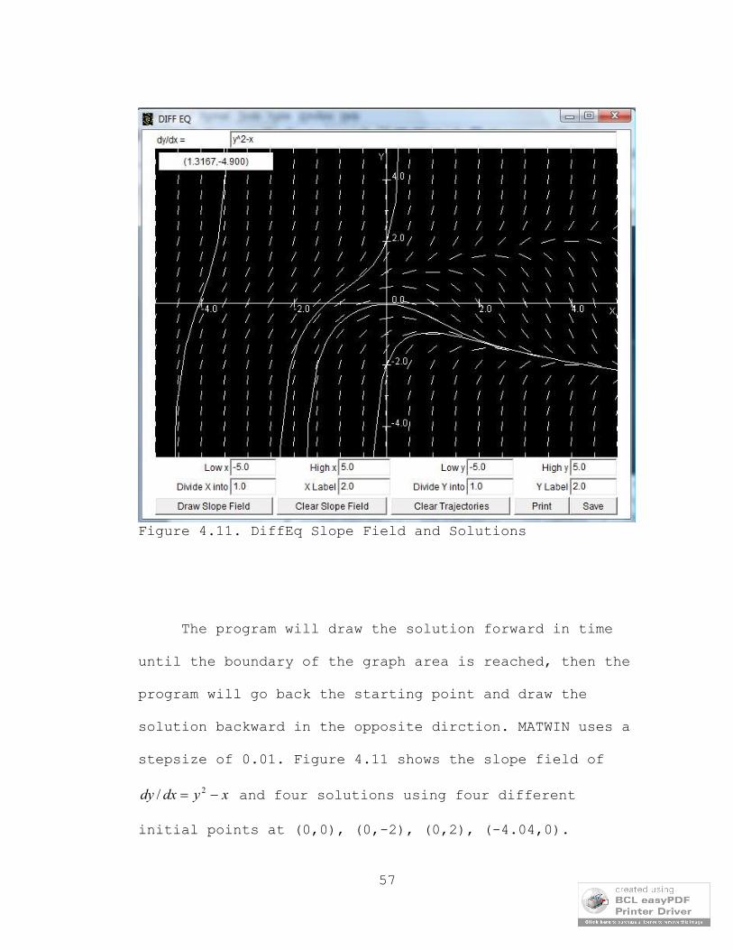
Figure 4.11. DiffEq Slope Field and Solutions

The program will draw the solution forward in time

until the boundary of the graph area is reached, then the

program will go back the starting point and draw the

solution backward in the opposite dirction. MATWIN uses a

stepsize of 0.01. Figure 4.11 shows the slope field of

xydxdy 2/ and four solutions using four different

initial points at (0,0), (0,-2), (0,2), (-4.04,0).

58

The situation is very similar with DiffEq, Phase

Plane program. The program draws slope field and the phse

plane solutions for the system of differential equations

represented by the two expression inserted into the

program. The solutions can be drawn by clicking the mouse

on the desired position in the grapgh area. Figure 4.12

shows a number of solutions (without the slope field

lines) drawn at a number of different initial points.

Figure 4.12. The Phase Plane solution trajectories

Saving And Printing

Saving and printing are similar in functionality the

Save and Print feaures discussed in the Analyzer section.

59

The only difference is that the images from DiffEq

program will be saved in a directory called DiffEq, and

those of the DiffEq, Phase Plane in a directory called

PhasePlane. Both directories are located in the

ImageFiles directory.

DiffEq, 3Dview

DiffEq, 3Dview is very interesting tool when it

comes to drawing the 3D-solution of the sytem of

differential equations of the form ),,(/ zyxfdtdx ,

),,(/ zyxgdtdy , and ),,(/ zyxhdtdz .

The DiffEq, 3Dview screen accepts three expressions

for dtdx / , dtdy / , and dtdz / . It contains fields to input

the desired values of the axes boundaries. To enable

utilizing the power of 3D graphics, the program has

optios to rotate, translate, and zoom the view displayed

in the grapgh area. There are three more fields labled

“_rot”, “y_rot”, and “z_rot”. These field are used to

input the desired angle values (in degrees) that the user

like to use to rotate the view arround the corresponding

axes. If x_rot is set to be 45, then pressing the button

“Draw” will redraw the scene after rotating it 45 degrees

60

arround x-axis. Compound rotations arround axed can be

done at one time, for example a rotation of 45 degrees

arround x-axis followed by another rotation of 30 degrees

arround y-axes can be done if x_rot is set to 45 and

y_rot is set to 30.

Figure 4.13. The view of the solution to 3 differentialEquations

61

Figure 4.13 shows the 3D view scene of the solution

of the differential equation system decribed by the

equations ydtdx / , xdtdx / , 2/ xdtdx . The coordinate of

the initial value are chosen by inserting them into the

fields xo, yo, and zo respectively. In the scene shown

above, xo is set to 1, yo and zo are boyh zeroes, which

means the initial point is (1,0,0). Also the values of

x_rot, y_rot, z_rot are all zeros, which means that there

is no rotation arround any axis. This is what made the

scene looks like two-dimensional scene.

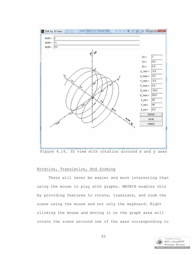
With a little change to the values in the x_rot and

y_rot data fields, the view will change to what we see in

figure 4.14. Notice how the view looks like a 3d-view

now.

62

Figure 4.14. 3D view with rotation arround x and y axes

Rotation, Translation, And Zooming

There will never be easier and more interesting than

using the mouse to play with graphs. MATWIN enables this

by providing features to rotate, translate, and zoom the

scene using the mouse and not only the keyboard. Right

clicking the mouse and moving it on the graph area will

rotate the scene arround one of the axes corresponding to

63

the motion. Also you can move (translate) the scene

within the graph area boundaries by left clicking on the

mouse and moving it. Also you can zoom the scene out and

in by right clicking and moving the mouse while holding

the “Alt” button pressed on the keyboard. Figure 4.15

shows the scene in figure 4.13 after being rotated,

translated, and zoomed out using the mouse.

Figure 4.15. Mouse rotation, translation, and zooming

64

Saving and Printing

Saving and printng in DiffEq, 3Dview is similar to

the saving and printing features in the rest of the

programs. The printed paper will look exactly as the view

on the screen. The image will be saved in aa folder

called 3DappletImages in the ImageFiles folder.

65

CHAPTER FIVE

CONCLUSION AND FUTUR EXTENSIONS

Summary

As we have seen, MATHWIN is an integrated piece of

software that consists of a number of graphics programs.

These programs are very efficient in dealing graphically

with certain systems of differential equations. It

provides the user with the ability to compute and

experiment the solutions of some complicated problems and

yet it does not require a wide knowledge of Math.

We showed how MATWIN provides tools for plotting

graphs of functions, graphs of derivatives, and tangents.

It also provides features for solving equations using

numerical methods, finding the roots, maxima and minima,

and calculating integrals.

The most powerful feature of MATWIN is the ability

to solve the differential equations and draw graphs of

these solutions. Its ability in solving differential

equations includes:

1. Solving differential equations of the form

),(/ yxfdxdy .

66

2. Solving systems of two differential equations of

the form ),(/ yxfdtdx , ),(/ yxgdtdy .

3. Solving systems of three differential equations

of the form ),,(/ zyxfdtdx , ),,(/ zyxfdtdy ,

),,(/ zyxfdtdz .

4. Drawing the slope fields and the trajectories of

the solutions of the above systems.

So MATWIN is very efficient tool that can accompany

the textbook for any differential equations course. Also

it can be of a great help to high school, and college

students who study calculus, since large portions of

calculus courses deal with roots, maxima and minima,

plotting graphs and finding integrals.

Program Evaluation

The program was tested using the following

procedures:

1. inserting a special code lines during the

development

The program. The purpose of these lines of code was

to output certain results that were used to check

the correctness of the program. This procedure has

67

been applied to each component separately, then was

applied one more time to the whole system after

integrating its components into one program. After

making sure that the program generates the expected

results, these lines of code were removed and the

program was compiled to generate the class files.

2. The graphs generated by MATWIN were checked against

those produced by MATLAB. The results ensured that

both graphs are equivalent in their outlook, the

points of intersection with the axes, at the

positions where the graphs show singularities.

Future Extensions

The heart of MATWIN lies in the “Equation” class.

This class includes all the methods to parse and evaluate

expressions. MATWIN can parse and evaluate any expression

that includes real numbers or variables that represent

real numbers. At this moment, it doesn’t support the

complex numbers in the form of bia , where a and b are

real numbers and i is the imaginary unit with the

property 12 i . Supporting complex numbers will have the

first priority in developing MATWIN.

68

Extending MATWIN ability to solve a wider range of

differential equations systems is another task that will

be having a great deal of attention in the future.

Also, making MATWIN available online on the World

Wide Web and allowing others to contribute to the

development of the software will be the next step in

developing MATWIN.

69

APPENDIX A

SAMPLE CODE

70

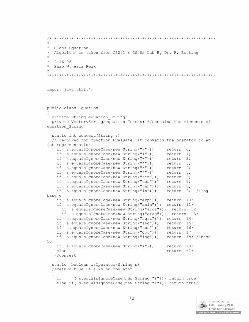
/********************************************************************** Class Equation* Algorithm is taken from CS201 & CS202 Lab By Dr. R. Botting** 9-16-06* Ehab W. Aziz Rezk*********************************************************************/

import java.util.*;

public class Equation{ private String equation_String; private Vector<String>equation_Tokens; //contains the elements of equation_String

static int convert(String s) // required for function Evaluate. it converts the operator to an int representation { if( s.equalsIgnoreCase(new String(")"))) return 0; if( s.equalsIgnoreCase(new String("+"))) return 1; if( s.equalsIgnoreCase(new String("-"))) return 2; if( s.equalsIgnoreCase(new String("*"))) return 3; if( s.equalsIgnoreCase(new String("/"))) return 4; if( s.equalsIgnoreCase(new String("^"))) return 5; if( s.equalsIgnoreCase(new String("sin"))) return 6; if( s.equalsIgnoreCase(new String("cos"))) return 7; if( s.equalsIgnoreCase(new String("tan"))) return 8; if( s.equalsIgnoreCase(new String("ln"))) return 9; //log base e if( s.equalsIgnoreCase(new String("exp"))) return 10; if( s.equalsIgnoreCase(new String("asin"))) return 11;

if( s.equalsIgnoreCase(new String("acos"))) return 12;if( s.equalsIgnoreCase(new String("atan"))) return 13;

if( s.equalsIgnoreCase(new String("sqrt"))) return 14; if( s.equalsIgnoreCase(new String("sec"))) return 15; if( s.equalsIgnoreCase(new String("csc"))) return 16; if( s.equalsIgnoreCase(new String("cot"))) return 17; if( s.equalsIgnoreCase(new String("log"))) return 18; //base 10 if( s.equalsIgnoreCase(new String("("))) return 20; else return -1; }//convert

static boolean isOperator(String s) //return true if s is an operator { if ( s.equalsIgnoreCase(new String(")"))) return true; else if( s.equalsIgnoreCase(new String("+"))) return true;

71

else if( s.equalsIgnoreCase(new String("-"))) return true; else if( s.equalsIgnoreCase(new String("*"))) return true; else if( s.equalsIgnoreCase(new String("/"))) return true; else if( s.equalsIgnoreCase(new String("^"))) return true; else if( s.equalsIgnoreCase(new String("("))) return true; else return false; }//isOperator

static boolean isOperator2(String s) //return true for sin, cos, tan, cot, sec. { if (s.equalsIgnoreCase(new String("sin")))return true; else if (s.equalsIgnoreCase(new String("cos")))return true; else if (s.equalsIgnoreCase(new String("tan")))return true; else if (s.equalsIgnoreCase(new String("cot")))return true; else if (s.equalsIgnoreCase(new String("sec")))return true; else if (s.equalsIgnoreCase(new String("csc")))return true; else if (s.equalsIgnoreCase(new String("log")))return true; else if (s.equalsIgnoreCase(new String("exp")))return true; else return false; }//isOprator2()

static boolean isOperator3(String s) //return true for ln { if (s.equalsIgnoreCase(new String("ln"))) return true; else return false; }//isOprator3()

static boolean isOperator4(String s) //return true for sqrt, asin, acos, atan { if (s.equalsIgnoreCase(new String("asin")))return true; else if (s.equalsIgnoreCase(new String("acos")))return true; else if (s.equalsIgnoreCase(new String("atan")))return true; else if (s.equalsIgnoreCase(new String("sqrt")))return true; else return false; }//isOprator4()

static boolean isNumber(char s) //return true for numbers { boolean returnValue=true;

{ if (s !='.' && s !='0' && s !='1' && s !='2' && s !='3' && s !='4' && s !='5' &&

s !='6' && s !='7' && s !='8' && s !='9'&& s !='x'&& s !='X' )

returnValue = false; } return returnValue; }//isnumber()

static void evaluate(Stack<Double> operand, Stack<String> oprator)

72

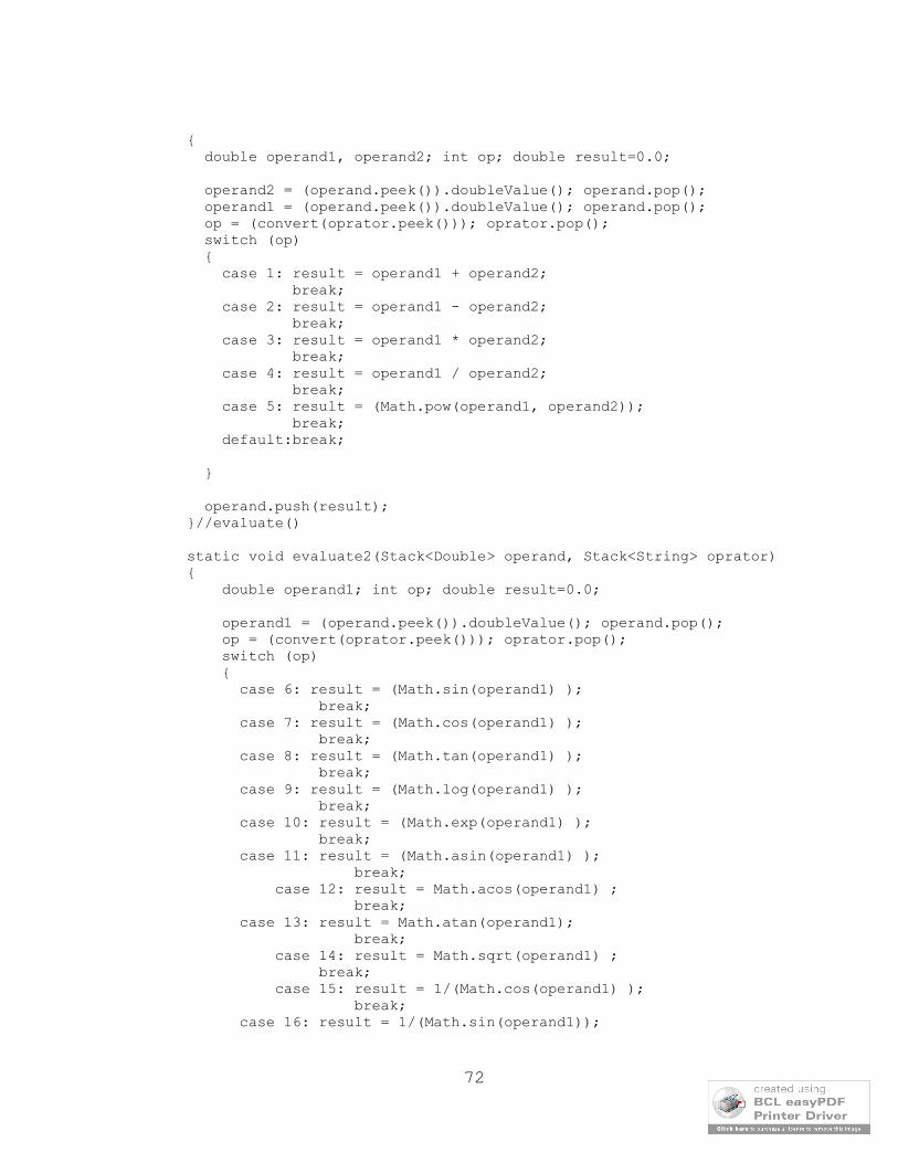
{ double operand1, operand2; int op; double result=0.0;

operand2 = (operand.peek()).doubleValue(); operand.pop(); operand1 = (operand.peek()).doubleValue(); operand.pop(); op = (convert(oprator.peek())); oprator.pop(); switch (op) { case 1: result = operand1 + operand2; break; case 2: result = operand1 - operand2; break; case 3: result = operand1 * operand2; break; case 4: result = operand1 / operand2; break; case 5: result = (Math.pow(operand1, operand2)); break; default:break;

}

operand.push(result); }//evaluate()

static void evaluate2(Stack<Double> operand, Stack<String> oprator) { double operand1; int op; double result=0.0;

operand1 = (operand.peek()).doubleValue(); operand.pop(); op = (convert(oprator.peek())); oprator.pop(); switch (op) { case 6: result = (Math.sin(operand1) ); break; case 7: result = (Math.cos(operand1) ); break; case 8: result = (Math.tan(operand1) ); break; case 9: result = (Math.log(operand1) ); break; case 10: result = (Math.exp(operand1) ); break; case 11: result = (Math.asin(operand1) );

break;case 12: result = Math.acos(operand1) ; break;

case 13: result = Math.atan(operand1); break;case 14: result = Math.sqrt(operand1) ;

break;case 15: result = 1/(Math.cos(operand1) ); break;

case 16: result = 1/(Math.sin(operand1));

73

break;case 17: result = 1/(Math.tan(operand1) ) ;

break;case 18: result = (Math.log(operand1) )/(Math.log(10) ) ;

break;//case 18 returns the log to the base 10 default: break;

}

operand.push(result); }//evaluate2()

static boolean isLetter(char s) {

//return true if s is letter boolean returnValue=true;

{ if (s !='a' && s !='A' && s !='b' && s !='B' && s !='c' && s !='C' && s !='d' &&

s !='D' && s !='e' && s !='E' && s !='f' && s !='F' && s !='g' && s !='G' &&

s !='h' && s !='H' && s !='i' && s !='I' && s !='j' && s !='J' && s !='k' &&

s !='K' && s !='l' && s !='L' && s !='m' && s !='M' && s !='n' && s !='N' &&

s !='o' && s !='O' && s !='p' && s !='P' && s !='q' && s !='Q' && s !='r' &&

s !='R' && s !='s' && s !='S' && s !='t' && s !='T' && s !='u' && s !='U' &&

s !='v' && s !='V' && s !='w' && s !='W' && s !='x' && s !='X' && s !='y' &&

s !='Y' && s !='z' && s !='Z') returnValue = false; }

return returnValue; }

/** The folowing function (vectorAdjust) is added to adjust the vector comming from class String to vector tokenizer it adjust equation like -sin.., -(...),... to (-1)*sin..,... this will enable the Evaluate function in the Equation class to correctly parse the expression to evaluate it It also replace e and pi by their mathematical values */ static Vector<String> vectorAdjust(Vector<String> vec) {

Vector<String> v =new Vector<String>(); v.add("("); v.add("-1"); v.add(")"); v.add("*"); if(vec.get(0).equals("-")) {

74

//if the leading character is a negative sine"-", replace it with "(-1)*"

vec.removeElementAt(0); vec.addAll(0,v);

} else{

for(int i=0;i<vec.size()-2; i++) {

if(vec.get(i).equals("(")&&vec.get(i+1).equals("-"))

{//if ( is followed by - change - to "(0-

1)*" vec.removeElementAt(i+1);

vec.addAll(i+1,v); }

else{} }

}//else return vec;

}

public Equation(String str) {//

equation_String = (str.trim()).concat("@");//adding @to the end

StringToVectorTokenizer stv = new StringToVectorTokenizer(str); Vector<String> v= vectorAdjust(stv.tokenizeToVector());//see function vetorAdjust for(int i=0; i<v.size(); i++) {

double e = Math.E; double pi =Math.PI;

if(v.get(i).equalsIgnoreCase("e")){

String s = Double.toString(e);v.set(i, s);

}else if(v.get(i).equalsIgnoreCase("-e")){

String s = "-".concat(Double.toString(e));v.set(i, s);

}else if(v.get(i).equalsIgnoreCase("pi")){

String s = Double.toString(pi);v.set(i, s);

}else if(v.get(i).equalsIgnoreCase("-pi")){

String s = "-".concat(Double.toString(pi));

75

v.set(i, s);}else{}

} equation_Tokens = v;

}//Equation(String)

public double Evaluate(String x, double d)//evaluate after substituting x with d {//return the double value of the euation_string Vector <String> temp = equation_Tokens; //a copyof the equation vector for(int i=0; i<temp.size(); i++) //replacing x with d {if((temp.elementAt(i)).equalsIgnoreCase(x)) temp.setElementAt( Double.toString(d),i); if((temp.elementAt(i)).equalsIgnoreCase("-"+x)&&d>0) temp.setElementAt( ("-"+Double.toString(d)),i); if((temp.elementAt(i)).equalsIgnoreCase("-"+x)&&d==0) temp.setElementAt( Double.toString(0),i); if((temp.elementAt(i)).equalsIgnoreCase("-"+x)&&d<0) temp.setElementAt( Double.toString(Math.abs(d)),i); }

Stack<Double> operand = new Stack<Double>(); Stack<String> oprator = new Stack<String>(); int op; //int equivallent of operator returned from convert String token = temp.firstElement() ;

for(int i=0; i< temp.size(); i++) { token = temp.elementAt(i); if(isOperator(token)||isOperator2(token)||isOperator3(token)||isOperator4(token)) { if (token.equalsIgnoreCase( ")")) { while(!(oprator.peek()).equalsIgnoreCase("(") ) {if(isOperator(oprator.peek()))evaluate(operand, oprator); else{evaluate2(operand, oprator);}

} oprator.pop(); //pop"(" } else { op = convert(token); while(!oprator.empty()&&!(oprator.peek()).equalsIgnoreCase("(") && op<=convert(oprator.peek())) {if(isOperator(oprator.peek()))evaluate(operand, oprator);

76

else{evaluate2(operand, oprator);} }

oprator.push(token); }//else }//if

else if(isNumber(token.charAt(0)) ) //token is a number operand.push(Double.valueOf(token).doubleValue());

else{operand.push(Double.valueOf(token).doubleValue());}

}//for

while (!oprator.empty()) {if(isOperator(oprator.peek()))evaluate(operand, oprator); else{evaluate2(operand, oprator);} }

return operand.peek();

}//Evaluate

public double Evaluate(double d1, double d2) //evaluate after substituting two variables x(first), y(seond) of the equation with d1 qand d2 { Vector <String> temp = equation_Tokens; //a copyof the equation vector ///////// for(int i=0; i<temp.size(); i++) //replacing x with d

{if((temp.elementAt(i)).equalsIgnoreCase("x")) temp.setElementAt( Double.toString(d1),i); if((temp.elementAt(i)).equalsIgnoreCase("-x")&&d1>0) temp.setElementAt( ("-"+Double.toString(d1)),i); if((temp.elementAt(i)).equalsIgnoreCase("-x")&&d1==0) temp.setElementAt( Double.toString(0),i); if((temp.elementAt(i)).equalsIgnoreCase("-x")&&d1<0) temp.setElementAt( Double.toString(Math.abs(d1)),i);

if((temp.elementAt(i)).equalsIgnoreCase("y")) temp.setElementAt( Double.toString(d2),i); if((temp.elementAt(i)).equalsIgnoreCase("-y")&&d2>0) temp.setElementAt( ("-"+Double.toString(d2)),i); if((temp.elementAt(i)).equalsIgnoreCase("-y")&&d2==0) temp.setElementAt( Double.toString(0),i); if((temp.elementAt(i)).equalsIgnoreCase("-y")&&d2<0) temp.setElementAt( Double.toString(Math.abs(d2)),i);

}

Stack<Double> operand = new Stack<Double>(); Stack<String> oprator = new Stack<String>();

77

int op; //int equivallent of operator returned from convert String token = temp.firstElement() ;

for(int i=0; i< temp.size(); i++) { token = temp.elementAt(i); if(isOperator(token)||isOperator2(token)||isOperator3(token)||isOperator4(token)) { if (token.equalsIgnoreCase( ")")) { while(!(oprator.peek()).equalsIgnoreCase("(") ) {if(isOperator(oprator.peek()))evaluate(operand, oprator); else{evaluate2(operand, oprator);}

} oprator.pop(); //pop"(" } else { op = convert(token); while(!oprator.empty()&&!(oprator.peek()).equalsIgnoreCase("(") && op<=convert(oprator.peek())) {if(isOperator(oprator.peek()))evaluate(operand, oprator); else{evaluate2(operand, oprator);}

} oprator.push(token); }//else }//if

else if(isNumber(token.charAt(0)) ) //token is a number operand.push(Double.valueOf(token).doubleValue());

else{operand.push(Double.valueOf(token).doubleValue());}

}//for

while (!oprator.empty()) {if(isOperator(oprator.peek()))evaluate(operand, oprator); else{evaluate2(operand, oprator);} }

return operand.peek();

}//Evaluate(double, double)

public double Evaluate(double d1, double d2, double d3) //evaluate after substituting two variables x(first), y(seond), z or t (third) //of the equation with d1 qand d2 and d3

78

{ Vector <String> temp = equation_Tokens; //a copyof the equation vector ///////// for(int i=0; i<temp.size(); i++) //replacing x with d

{if((temp.elementAt(i)).equalsIgnoreCase("x")) temp.setElementAt( Double.toString(d1),i); if((temp.elementAt(i)).equalsIgnoreCase("-x")&&d1>0) temp.setElementAt( ("-"+Double.toString(d1)),i); if((temp.elementAt(i)).equalsIgnoreCase("-x")&&d1==0) temp.setElementAt( Double.toString(0),i); if((temp.elementAt(i)).equalsIgnoreCase("-x")&&d1<0) temp.setElementAt( Double.toString(Math.abs(d1)),i);

if((temp.elementAt(i)).equalsIgnoreCase("y")) temp.setElementAt( Double.toString(d2),i); if((temp.elementAt(i)).equalsIgnoreCase("-y")&&d2>0) temp.setElementAt( ("-"+Double.toString(d2)),i); if((temp.elementAt(i)).equalsIgnoreCase("-y")&&d2==0) temp.setElementAt( Double.toString(0),i); if((temp.elementAt(i)).equalsIgnoreCase("-y")&&d2<0) temp.setElementAt( Double.toString(Math.abs(d2)),i);

if((temp.elementAt(i)).equalsIgnoreCase("z")) temp.setElementAt( Double.toString(d3),i); if((temp.elementAt(i)).equalsIgnoreCase("-z")&&d3>0) temp.setElementAt( ("-"+Double.toString(d3)),i); if((temp.elementAt(i)).equalsIgnoreCase("-z")&&d3==0) temp.setElementAt( Double.toString(0),i); if((temp.elementAt(i)).equalsIgnoreCase("-z")&&d3<0) temp.setElementAt( Double.toString(Math.abs(d3)),i);

}

Stack<Double> operand = new Stack<Double>(); Stack<String> oprator = new Stack<String>(); int op; //int equivallent of operator returned from convert String token = temp.firstElement() ;

for(int i=0; i< temp.size(); i++) { token = temp.elementAt(i); if(isOperator(token)||isOperator2(token)||isOperator3(token)||isOperator4(token)) { if (token.equalsIgnoreCase( ")")) { while(!(oprator.peek()).equalsIgnoreCase("(") ) {if(isOperator(oprator.peek()))evaluate(operand, oprator);

79

else{evaluate2(operand, oprator);} }

oprator.pop(); //pop"(" } else { op = convert(token); while(!oprator.empty()&&!(oprator.peek()).equalsIgnoreCase("(") && op<=convert(oprator.peek())) {if(isOperator(oprator.peek()))evaluate(operand, oprator); else{evaluate2(operand, oprator);}

} oprator.push(token); }//else }//if

else if(isNumber(token.charAt(0)) ) //token is a number operand.push(Double.valueOf(token).doubleValue());

else{operand.push(Double.valueOf(token).doubleValue());}

}//for

while (!oprator.empty()) {if(isOperator(oprator.peek()))evaluate(operand, oprator); else{evaluate2(operand, oprator);} }

return operand.peek();

}//Evaluate(double, double) public void print_equation_Tokens() { System.out.print("\n"); for(int i=0; i<equation_Tokens.size()-1; i++) System.out.print(equation_Tokens.get(i) +", " ); System.out.print(equation_Tokens.lastElement() +"\n"); }

public String get_equation_String() { return equation_String; }

public Vector<String> get_equation_Tokens() { return equation_Tokens; }

80

public static void main(String[ ] args) {

} //main

}//Equation class

81

/********************************************************************** Class DerivativeFinder* 9-16-06* Ehab W. Aziz Rezk*********************************************************************/

import java.util.*;

public class DerivativeFinder{

private String classString; //the eqquation ehose derivative is to be calcuated

private Vector<String>stringTokens;

public DerivativeFinder(String s){

classString = s.trim();

StringToVectorTokenizer stv = new StringToVectorTokenizer(s);

stringTokens = stv.tokenizeToVector();

}//public derivativeFinder(s)

//the following function answe fix adjust the answer if it has term multiplied

// or added to 0. ((ln((x-3)))*(0)))--> ((0))static String answerFix(String s){

String temp = s;int g=0;while(g<s.length()){

if(((s.length()>=4)&&s.substring(g, g+4).equals("+(0)"))||

((s.length()>=4)&&s.substring(g, g+4).equals("-(0)")))

{String one = s.substring(0,g);String two= s.substring(g+4);return one.concat(two);

}else if((s.length()>=5)&&s.substring(g,

g+5).equals("*(0))")){

int counter=-1;for(int l=g-1; l>=0;l--){

if(s.charAt(l)==')')counter--;

82

else if(s.charAt(l)=='(')counter++;else{}

if(counter==0){

String one = s.substring(0,l).concat("(0)");

String two= s.substring(g+5);return one.concat(two);

}}

}

g++;}return s;

}//answerFix

static boolean isOperator(String s)//return true if s is an operator{ if ( s.equalsIgnoreCase(new String(")"))) return true; else if( s.equalsIgnoreCase(new String("+"))) return true; else if( s.equalsIgnoreCase(new String("-"))) return true; else if( s.equalsIgnoreCase(new String("*"))) return true; else if( s.equalsIgnoreCase(new String("/"))) return true; else if( s.equalsIgnoreCase(new String("^"))) return true; else if( s.equalsIgnoreCase(new String("("))) return true; else return false;}//isOperator

static boolean isOperator2(String s)//return true for sin, cos, tan, cot, sec.{ if (s.equalsIgnoreCase(new String("sin")))return

true; else if (s.equalsIgnoreCase(new String("cos")))return

true; else if (s.equalsIgnoreCase(new String("tan")))return

true; else if (s.equalsIgnoreCase(new String("cot")))return

true; else if (s.equalsIgnoreCase(new String("sec")))return

true; else if (s.equalsIgnoreCase(new String("csc")))return

true; else if (s.equalsIgnoreCase(new String("log")))return

true; else if (s.equalsIgnoreCase(new String("exp")))return

true; else return

false;}//isOprator2()

83

static boolean isOperator3(String s)//return true for ln{ if (s.equalsIgnoreCase(new String("ln"))) return

true; else return

false;}//isOprator3()

static boolean isOperator4(String s)//return true for sqrt, asin, acos, atan{ if (s.equalsIgnoreCase(new String("asin")))return

true; else if (s.equalsIgnoreCase(new String("acos")))return

true; else if (s.equalsIgnoreCase(new String("atan")))return

true; else if (s.equalsIgnoreCase(new String("acot")))return

true; else if (s.equalsIgnoreCase(new String("asec")))return

true; else if (s.equalsIgnoreCase(new String("acsc")))return

true; else if (s.equalsIgnoreCase(new String("sqrt")))return

true; else return

false;}//isOprator4()

static boolean isNumber(char s)//return true for numbers{ boolean returnValue=true;

{ if (s !='.' && s !='0' && s !='1' && s !='2' && s !='3' && s !='4' && s !='5' &&

s !='6' && s !='7' && s !='8' && s !='9'&& s !='x'&& s !='X' )

returnValue = false; } return returnValue;}//isnumber()

static boolean isPNumber(String s){ s.trim(); boolean returnValue = true; for(int i =0;i<s.length();i++)

{if(!isNumber(s.charAt(i))) returnValue=false;

}

return returnValue;}

84

static boolean isNNumber(String s){ s.trim();

if(s.charAt(0)=='-'&& isPNumber(s.substring(1)))return true;

else return false;

}

static boolean isNumber(String s) {

if(isNNumber(s)||isPNumber(s)) return true;else return false;

}

/** The folowing function (vectorAdjust) is added to adjust the vector comming from class String to vector tokenizer it adjust equation like -sin.., -(...),... to (-1)*sin..,... this will enable the Evaluate function in the Equation class to correctly parse the expression to evaluate it */ static Vector<String> vectorAdjust(Vector<String> vec) {

Vector<String> v =new Vector<String>(); v.add("("); v.add("-1"); v.add(")"); v.add("*"); if(vec.get(0).equals("-")) {

//if the leading character is a negative sine"-", replace it with "(-1)*"

vec.removeElementAt(0); vec.addAll(0,v); return vec;

} else{

for(int i=0;i<vec.size()-2; i++) {

if(vec.get(i).equals("(")&&vec.get(i+1).equals("-"))

{ //if ( is followed by - change - to "(0-

1)*" vec.removeElementAt(i+1);

vec.addAll(i+1,v); return vec;

} else{}

} return vec; }//else

}

public void print_stringTokens()

85

{ System.out.print("\n"); for(int i=0; i<stringTokens.size()-1; i++) System.out.print(stringTokens.get(i) +", " ); System.out.print(stringTokens.lastElement() +"\n");}

public String get_equation_String(){ return classString;}

public Vector<String> get_stringTokens(){ return stringTokens;

}

public static void printVector(Vector<String> vec){ System.out.print("\n"); for(int i=0; i<vec.size()-1; i++) System.out.print(vec.get(i) +", " ); System.out.print(vec.lastElement() +"\n");}public static Vector<String> getVectorFrom(Vector<String> vec,

int from, int until){//return another vector which is a part of the current vector //bound from "from"index to "untill" index

Vector<String>temp = new Vector<String> (); for(int i = from; i<=until;i++) {

temp.addElement(vec.get(i)); } return temp;

}

public static String vectorToString(Vector<String> vec){

String s = ""; for(int i=0; i<vec.size(); i++) s=s.concat(vec.get(i)); return s;

}/****/

static public String findDerivative(Vector<String> vec)//find derivative of class string located in class vector {

Vector<String> vector = vectorAdjust(vec);

if(vector.get(0).equals("(")&&vector.lastElement().equals(")")){

86

//removing the frame (......) or((..)(..))but not the one like (..)(..)

//by cheking inside the frame if ) is found befor ( or not

int j=0; //bracket open and close counterboolean bracket = true;for(int k=1; k<vector.size()-1;k++){

if(vector.get(k).equals("("))j+=1;else if(vector.get(k).equals(")"))j-=1;else{}if(j<0) bracket = false;

}if(bracket)return

findDerivative(getVectorFrom(vector, 1, vector.size()-2));else{}

}

if(vector.size()==0){

String ret = "there is no equation to differentiate."; return ret;

} else if(vector.size()==1)//expression is X or constant number

{if(vector.get(0).equalsIgnoreCase("x")) return

"1";else if(vector.get(0).equalsIgnoreCase("-x"))

return "-1";else if(isNumber(vector.get(0))) return "0";else

if(vector.get(0).equalsIgnoreCase("e")||vector.get(0).equalsIgnoreCase("-e")) return "0";

else if(vector.get(0).equalsIgnoreCase("pi")||vector.get(0).equalsIgnoreCase("-pi")) return "0";

else{return "expression not suported";}}else if(vector.size()==2)//sinX, sqrtX, sin30, cos -x,...{

if(vector.get(0).equalsIgnoreCase("sin")&& vector.get(1).equalsIgnoreCase("x")) return "(cos x)";

else if(vector.get(0).equalsIgnoreCase("sin")&& vector.get(1).equalsIgnoreCase("-x")) return "(-cos -x)";

else if(vector.get(0).equalsIgnoreCase("sin")&& isNumber(vector.get(1))) return "0";

else if(vector.get(0).equalsIgnoreCase("cos")&& vector.get(1).equalsIgnoreCase("x")) return "(-sin x)";

else if(vector.get(0).equalsIgnoreCase("cos")&& vector.get(1).equalsIgnoreCase("-x")) return "(sin -x)";

else if(vector.get(0).equalsIgnoreCase("cos")&& isNumber(vector.get(1))) return "0";

87

else if(vector.get(0).equalsIgnoreCase("tan")&& vector.get(1).equalsIgnoreCase("x")) return "((sec x)^2)";

else if(vector.get(0).equalsIgnoreCase("tan")&& vector.get(1).equalsIgnoreCase("-x")) return "(-(sec -x)^2)";

else if(vector.get(0).equalsIgnoreCase("tan")&& isNumber(vector.get(1))) return "0";

else if(vector.get(0).equalsIgnoreCase("sec")&& vector.get(1).equalsIgnoreCase("x")) return "((sec x)*(tan x))";

else if(vector.get(0).equalsIgnoreCase("sec")&& vector.get(1).equalsIgnoreCase("-x")) return "(-(sec -x)*(tan -x))";

else if(vector.get(0).equalsIgnoreCase("sec")&& isNumber(vector.get(1))) return "0";

else if(vector.get(0).equalsIgnoreCase("csc")&& vector.get(1).equalsIgnoreCase("x")) return "(-(csc x)*(cot x))";

else if(vector.get(0).equalsIgnoreCase("csc")&& vector.get(1).equalsIgnoreCase("-x")) return "((csc -x)*(cot -x))";

else if(vector.get(0).equalsIgnoreCase("csc")&& isNumber(vector.get(1))) return "0";

else if(vector.get(0).equalsIgnoreCase("cot")&& vector.get(1).equalsIgnoreCase("x")) return "(-(csc x)^2)";

else if(vector.get(0).equalsIgnoreCase("cot")&& vector.get(1).equalsIgnoreCase("-x")) return "((csc x)^2)";

else if(vector.get(0).equalsIgnoreCase("cot")&& isNumber(vector.get(1))) return "0";

else if(vector.get(0).equalsIgnoreCase("asin")&& vector.get(1).equalsIgnoreCase("x")) return "(1/sqrt(1-(x^2)))";

else if(vector.get(0).equalsIgnoreCase("asin")&& vector.get(1).equalsIgnoreCase("-x")) return "(-1/sqrt(1-(x^2)))";

else if(vector.get(0).equalsIgnoreCase("asin")&& isNumber(vector.get(1))) return "0";

else if(vector.get(0).equalsIgnoreCase("acos")&& vector.get(1).equalsIgnoreCase("x")) return "(-1/sqrt(1-(x^2)))";

else if(vector.get(0).equalsIgnoreCase("acos")&& vector.get(1).equalsIgnoreCase("-x")) return "(1/sqrt(1-(x^2)))";

else if(vector.get(0).equalsIgnoreCase("acos")&& isNumber(vector.get(1))) return "0";

else if(vector.get(0).equalsIgnoreCase("atan")&& vector.get(1).equalsIgnoreCase("x")) return "(1/(1+(x^2)))";

else if(vector.get(0).equalsIgnoreCase("atan")&& vector.get(1).equalsIgnoreCase("-x")) return "(-1/(1+(x^2)))";

else if(vector.get(0).equalsIgnoreCase("atan")&& isNumber(vector.get(1))) return "0";

else if(vector.get(0).equalsIgnoreCase("asec")&& vector.get(1).equalsIgnoreCase("x")) return "(1/(x*sqrt((x^2)-1)))";

else if(vector.get(0).equalsIgnoreCase("asec")&& vector.get(1).equalsIgnoreCase("-x")) return "(-1/(x*sqrt((x^2)-1)))";

88

else if(vector.get(0).equalsIgnoreCase("asec")&& isNumber(vector.get(1))) return "0";

else if(vector.get(0).equalsIgnoreCase("exp")&& vector.get(1).equalsIgnoreCase("x")) return "(expx)";

else if(vector.get(0).equalsIgnoreCase("exp")&& vector.get(1).equalsIgnoreCase("-x")) return "(-exp(-x))";

else if(vector.get(0).equalsIgnoreCase("exp")&& isNumber(vector.get(1))) return "0";

else if(vector.get(0).equalsIgnoreCase("ln")&& vector.get(1).equalsIgnoreCase("x")) return "(1/x)";

else if(vector.get(0).equalsIgnoreCase("ln")&& vector.get(1).equalsIgnoreCase("-x")) return "(1/x)";

else if(vector.get(0).equalsIgnoreCase("ln")&& isNumber(vector.get(1))) return "0";

else if(vector.get(0).equalsIgnoreCase("log")&& vector.get(1).equalsIgnoreCase("x")) return "(1/(x*ln(10)))";

else if(vector.get(0).equalsIgnoreCase("log")&& vector.get(1).equalsIgnoreCase("-x")) return "(1/(x*ln(10)))";

else if(vector.get(0).equalsIgnoreCase("log")&& isNumber(vector.get(1))) return "0";

else if(vector.get(0).equalsIgnoreCase("sqrt")&& vector.get(1).equalsIgnoreCase("x")) return "(1/(2*sqrtx))";

//sqrt is not defined or -veelse if(vector.get(0).equalsIgnoreCase("sqrt")&&

isNumber(vector.get(1))) return "0";

else{return "expression not suported";}}

else //recursive cals{

boolean state=true; //for +,-boolean state2=true; //for *,/boolean state3=true; //for ^boolean state4=true; //for sin cos,exp,....int i=0;//bracket tracerint k = 0;//while terminatorwhile(state){

if(vector.get(k).equals("(")){ i+=1; k+=1;}else if(vector.get(k).equals(")")) {i-=1;

k+=1;}else if(vector.get(k).equals("+")&&

i==0)//...+...{

state2=false; //block the next while block

state3=false; state4=false;String s=

findDerivative(getVectorFrom(vector, 0, k-1)).concat("+").concat

89

(findDerivative(getVectorFrom(vector, k+1, vector.size()-1)) );

return "(".concat(s).concat(")");

}else if(vector.get(k).equals("-")&&

i==0)//...-...{

state2=false; //block the next while block

state3=false; state4=false;String s=

findDerivative(getVectorFrom(vector, 0, k-1)).concat("-").concat

(findDerivative(getVectorFrom(vector, k+1, vector.size()-1)) );return "(".concat(s).concat(")");

}else{ k+=1; }

if(k==vector.size()-1) state = false;

}k=0;i=0;while(state2)//if + or - not detected in the first

part this part will work{

if(vector.get(k).equals("(")){ i+=1; k+=1;}else if(vector.get(k).equals(")")) {i-=1;

k+=1;}else if(vector.get(k).equals("*")&&

i==0)//...*...{

state3=false; state4=false;Vector<String> term1 =

getVectorFrom(vector, 0, k-1); //first termVector<String> term2 =

getVectorFrom(vector, k+1, vector.size()-1);//second term//s1=first*d(second)String

s1="(".concat(vectorToString(term1)).concat(")").concat("*").concat("(")

.concat(findDerivative(term2)).concat(")");

//s2= second *d(first)String

s2="(".concat(vectorToString(term2)).concat(")").concat("*").concat("(")

.concat(findDerivative(term1)).concat(")");

return "((".concat(s1).concat(")").concat("+").concat("(").concat(s2).concat("))");

}

90

else if(vector.get(k).equals("/")&& i==0){

state3=false; state4=false;Vector<String> num =

getVectorFrom(vector, 0, k-1); //numerator and denomeratorVector<String> den =

getVectorFrom(vector, k+1, vector.size()-1); // denomenator

String s1 = vectorToString(den).concat("*").concat(findDerivative(num)) ;

String s2 = vectorToString(num).concat("*").concat(findDerivative(den)) ;

String s3 = "(".concat(vectorToString(den)).concat(")^2");

return "(((".concat(s1).concat(")").concat("-").concat("(").concat(s2).concat("))/(").concat(s3).concat("))");

}//else ifelse{ k+=1;}if(k==vector.size()-1) state2=false;

}k=0;i=0;while(state3)//if * 0r / not detected in the first

part this part will work{ //u^v

if(vector.get(k).equals("(")){ i+=1; k+=1;}else if(vector.get(k).equals(")")) {i-=1;

k+=1;}else if(vector.get(k).equals("^")&&

i==0)//...*...{

state4=false;Vector<String> term1 =

getVectorFrom(vector, 0, k-1); //first termVector<String> term2 =

getVectorFrom(vector, k+1, vector.size()-1);//second term

if(term2.size()==1&&isNumber(term2.get(0))&&!("x").equalsIgnoreCase(term2.get(0)))

{double t2 =

Double.valueOf(term2.get(0).trim()).doubleValue();String p = Double.toString(t2);

//powerString pm1 = Double.toString(t2-

1); //power-1

String s1="(".concat(p).concat("*").concat("(").concat(vectorToString(term1))

.concat("^").concat(pm1).concat("))");

91

String s2 = findDerivative(term1);

return "(".concat(s1).concat("*").concat(s2).concat(")");

}else{//s1=(first^second)String

s1="((".concat(vectorToString(term1)).concat(")").concat("^").concat("(")

.concat(vectorToString(term2)).concat("))");

//s2= (second*d(first)/first)String s2=

"(((".concat(vectorToString(term2)).concat(")").concat("*").concat("(")

.concat(findDerivative(term1)).concat("))")

.concat("/").concat("(").concat(vectorToString(term1)).concat("))");

//s3 = ln(first)*d(second)String s3=

"(".concat("(ln(").concat(vectorToString(term1)).concat("))*(")

.concat(findDerivative(term2)).concat("))");String

s4="(".concat(s2).concat("+").concat(s3).concat(")");

String strin= "(".concat(s1).concat("*").concat(s4).concat(")");

//fixing the ln part when multiplied by 0return strin;

}}

//else ifelse{ k+=1;}if(k==vector.size()-1) state3=false;

}k=0;i=0;while(state4)//if = or - not detected in the first

part this part will work{

if(vector.get(k).equalsIgnoreCase("sin"))//sin...-->cos{

state4=false;Vector<String> term =

getVectorFrom(vector, k+1, vector.size()-1);return

"((cos(".concat(vectorToString(term)).concat("))").concat("*(")

92

.concat(findDerivative(term)).concat("))");

}else

if(vector.get(k).equalsIgnoreCase("cos"))//cos....-->-sin{

state4=false;Vector<String> term =

getVectorFrom(vector, k+1, vector.size()-1);return "((-

sin(".concat(vectorToString(term)).concat("))").concat("*(")

.concat(findDerivative(term)).concat("))");}else

if(vector.get(k).equalsIgnoreCase("tan"))//tan...--> sec square.{

state4=false;Vector<String> term =

getVectorFrom(vector, k+1, vector.size()-1);return

"(((sec(".concat(vectorToString(term)).concat("))").concat("^2)").concat("*(")

.concat(findDerivative(term)).concat("))");

}else

if(vector.get(k).equalsIgnoreCase("cot"))//cot...-->-csc square{

state4=false;Vector<String> term =

getVectorFrom(vector, k+1, vector.size()-1);return "((-

(csc(".concat(vectorToString(term)).concat("))").concat("^2)").concat("*(")

.concat(findDerivative(term)).concat("))");

}else

if(vector.get(k).equalsIgnoreCase("sec"))//sec...-->sec tan{

state4=false;Vector<String> term =

getVectorFrom(vector, k+1, vector.size()-1);return

"(((sec(".concat(vectorToString(term)).concat("))")

.concat("*(tan(").concat(vectorToString(term)).concat(")))")

.concat("*(").concat(findDerivative(term)).concat("))");}else

if(vector.get(k).equalsIgnoreCase("csc"))//csc...-->-csc cot{

93

state4=false;Vector<String> term =

getVectorFrom(vector, k+1, vector.size()-1);return "((-

(csc(".concat(vectorToString(term)).concat("))")

.concat("*(cot(").concat(vectorToString(term)).concat(")))")

.concat("*(").concat(findDerivative(term)).concat("))");}else

if(vector.get(k).equalsIgnoreCase("asin"))//asin..-->1/sqrt(1-x^2){

state4=false;Vector<String> term =

getVectorFrom(vector, k+1, vector.size()-1);return

"((1/(".concat("sqrt(").concat("1-((").concat(vectorToString(term))

.concat(")^2))))").concat("*(").concat(findDerivative(term)).concat("))");

}else

if(vector.get(k).equalsIgnoreCase("acos"))//acos..-->-1/sqrt(1-x^2){

state4=false;Vector<String> term =

getVectorFrom(vector, k+1, vector.size()-1);return "((-

1/(".concat("sqrt(").concat("1-((").concat(vectorToString(term))

.concat(")^2))))").concat("*(").concat(findDerivative(term)).concat("))");

}else

if(vector.get(k).equalsIgnoreCase("atan"))//atan..-->1/(1+x^2){

state4=false;Vector<String> term =

getVectorFrom(vector, k+1, vector.size()-1);return

"((1/".concat("(1+((").concat(vectorToString(term))

.concat(")^2)))").concat("*(").concat(findDerivative(term)).concat("))");

}else

if(vector.get(k).equalsIgnoreCase("asec"))//asec-->1/x*sqrt(x^2-1){

state4=false;Vector<String> term =

getVectorFrom(vector, k+1, vector.size()-1);return

"((1/((".concat(vectorToString(term)).concat(")*(sqrt(((")

94

.concat(vectorToString(term)).concat(")^2)-1))))")

.concat("*(").concat(findDerivative(term)).concat("))");

}else

if(vector.get(k).equalsIgnoreCase("exp"))//expx -->expx....{

state4=false;Vector<String> term =

getVectorFrom(vector, k+1, vector.size()-1);return

"((exp(".concat(vectorToString(term)).concat("))*(")

.concat(findDerivative(term)).concat("))");}else

if(vector.get(k).equalsIgnoreCase("ln"))//lnx-->1/x{

state4=false;Vector<String> term =

getVectorFrom(vector, k+1, vector.size()-1);return

"((1/(".concat(vectorToString(term)).concat("))*(")

.concat(findDerivative(term)).concat("))");}else

if(vector.get(k).equalsIgnoreCase("log"))//log-->1/(x*ln10){

state4=false;Vector<String> term =

getVectorFrom(vector, k+1, vector.size()-1);return

"((1/((".concat(vectorToString(term)).concat(")*(ln(10))))*(")

.concat(findDerivative(term)).concat("))");}else

if(vector.get(k).equalsIgnoreCase("sqrt"))//sqrt-->1/(2*sqrtx){

state4=false;Vector<String> term =

getVectorFrom(vector, k+1, vector.size()-1);return

"((1/(2*(sqrt(".concat(vectorToString(term)).concat("))))")

.concat("*(").concat(findDerivative(term)).concat("))");}

else{ k+=1;}if(k==vector.size()-1) state4=false;

}

95

}//else return" more rules";

}//findDerivative(..)

public static void main(String[ ] args) {

}//main

}//class derivativeFinder

96

/********************************************************************** Class MaxMinFinder* Ehab W. Aziz Rezk*********************************************************************/import java.util.*;

public class MaxMinFinder{

private String expression; //the equationprivate String firstDerivative;private String secondDerivative;

public MaxMinFinder(String str){

expression = str;

DerivativeFinder df1 = new DerivativeFinder(expression);StringToVectorTokenizer stv1 = new

StringToVectorTokenizer(expression);Vector<String> ve = stv1.tokenizeToVector();firstDerivative = df1.findDerivative(ve);

DerivativeFinder df2 = new DerivativeFinder(expression);StringToVectorTokenizer stv2 = new

StringToVectorTokenizer(firstDerivative);ve = stv2.tokenizeToVector();secondDerivative = df2.findDerivative(ve);

}

public String retExpression() {

return expression;}public String ret1st(){

return firstDerivative;}public String ret2nd(){

return secondDerivative;}

/* findMaxMin(..) where from and to are the boundary of the range through which the maxima and minima are to be found. step is the amount by which the function devides the region to find the roots, eps is the accuracy of finding the roots

97

**/public Vector<String> findMaxMin(double from, double to, double

step, double eps ){

RootFinder rf = new RootFinder(firstDerivative, eps);Vector<String> vec = rf.findAllRoots(from, to, step);return vec;

}

public static void main(String[ ] args){

Scanner sc = new Scanner(System.in);System.out.print("write down the Equation ");

String equation =sc.nextLine(); MaxMinFinder mf1 = new MaxMinFinder(equation);

String firstd = mf1.ret1st(); String secondd = mf1.ret2nd();

Equation eq1 = new Equation(firstd); Equation eq2 = new Equation(secondd);

Scanner sc2 = new Scanner(System.in);System.out.println("for x = ");String input =sc2.nextLine();

double value = Double.valueOf(input.trim()).doubleValue();

String x="x"; System.out.println("\n 1st = " +eq1.Evaluate(x, value)); System.out.println("\n 2nd = " +eq2.Evaluate(x, value));

System.out.println("a = "); Scanner sc3 = new Scanner(System.in); String a =sc3.nextLine(); System.out.println("b = "); Scanner sc4 = new Scanner(System.in); String b =sc4.nextLine(); double from =Double.valueOf(a.trim()).doubleValue(); double to = Double.valueOf(b.trim()).doubleValue(); Vector<String> v= mf1.findMaxMin( from, to, 1, 0.0001 ); for(int i=0; i<v.size();i++) System.out.print(v.get(i)+" ,");

}//main}

98

/****************************************************************** Class RootFinder****************************************************************/import java.util.*;

public class RootFinder{

static double midValue(double x1, double x2){

//return the mid value of x1 and x2return (x1+x2)/2;

}static double abs(double a){

//returns the absolute value of aif(a==0.0)return 0.0;else if(a>0.0) return a;else return -1*a;

}static boolean almostequals(double a, double b){

if(abs(a-b)<0.009)return true;else return false;

}

private String expression; //the equationprivate double epsilon;

public RootFinder(String str, double eps){

expression=str;epsilon = eps;//the accuracy in determining the root

}//public RootFinder()

public double Evaluate(double a){

Equation e= new Equation(expression);return e.Evaluate("x", a);

}public String firstDerivative(){

//return first derivative of expressionDerivativeFinder df1 = new DerivativeFinder(expression);StringToVectorTokenizer stv1 = new

StringToVectorTokenizer(expression);Vector<String> ve = stv1.tokenizeToVector();

99

return df1.findDerivative(ve);}public String secondDerivative(){

//returns the second derivative of expressionDerivativeFinder df1 = new DerivativeFinder(expression);StringToVectorTokenizer stv1 = new

StringToVectorTokenizer(expression);Vector<String> ve = stv1.tokenizeToVector();String fd= df1.findDerivative(ve);

DerivativeFinder df2 = new DerivativeFinder(expression);StringToVectorTokenizer stv2 = new

StringToVectorTokenizer(fd);ve = stv2.tokenizeToVector();return df2.findDerivative(ve);

}public double fDEvaluate( double a){

//return the double value of the 2nd derivativeString firstDerivative = firstDerivative();Equation eq= new Equation(firstDerivative);return eq.Evaluate("x", a);

}public double sDEvaluate( double a){

//return the double value of the 2nd derivativeString secondDerivative = secondDerivative();Equation eq= new Equation(secondDerivative);return eq.Evaluate("x", a);

}

boolean theFuncSlopeChange(double x1, double x2){

//return true if the function slope change between x1, x2if((fDEvaluate(x1)*fDEvaluate(x2))<0)return true;else return false;

}

boolean theCurveCrossX(double x1, double x2){

//return true if the root lies between x1 and x2//i.e.. the function has different signs on both

ddirectionsdouble value1 = Evaluate(x1);double value2 =

Evaluate(x2);

if((value1<0.0&&value2>0.0)||(value1>0.0&&value2<0.0))return true;//they are dif in signs

else return false;}//find all roots in the interval[v1, v2]taking a step Stepppublic Vector<String> findAllRoots(double v1, double v2,

double stepp)

100

{Vector<String> vector = new Vector<String>();//the vector

that carries the roots if foundvector.add("");int n=0; //number of times y is +veint m=0; //number of times y = -vefor(double k=v1; k<=v2+0.1; k+=stepp){

if(Evaluate(k)==0.0)vector.add(Double.toString(k));else if(Evaluate(k)>0.0)n++;else {m++;} //if(Evaluate(k)<0.0)m++;

if(n>0&&m>0)//there is crossing{

String root =findRootByBisection(k-stepp, k+stepp);

vector.add(root);m=0;n=0;

}

}for(double k=v1; k<=v2+0.1; k+=stepp)//only detext the

touch points{

if(Evaluate(k-stepp)>0&&Evaluate(k+stepp)>0 &&fDEvaluate(k-stepp)<0&&fDEvaluate(k+stepp)>0)

{String root = findRootByNewton(k);if(!(root.equals("no root

exist"))&&(Double.valueOf(root).doubleValue()>=v1&&

Double.valueOf(root).doubleValue()<=v2))vector.add(root);

}if(Evaluate(k-stepp)<0&&Evaluate(k+stepp)<0

&&fDEvaluate(k-stepp)>0&&fDEvaluate(k+stepp)<0){

String root = findRootByNewton(k);if(!(root.equals("no root

exist"))&&(Double.valueOf(root).doubleValue()>=v1&&

Double.valueOf(root).doubleValue()<=v2))vector.add(root);

}}//adjustiing the vector to be returnedif(vector.size()==1&&vector.get(0).equals(""))

vector.set(0, "NaN");else vector.remove(0);Vector<Double> vect = new Vector<Double>();for(int l=0; l<vector.size();l++){

if(vector.get(l).equals("no root exist")||vector.get(l).equals(""))

101

vector.remove(l);}for(int l=0; l<vector.size()-1;l++){

double d1=Double.valueOf(vector.get(l)).doubleValue();

double d2=Double.valueOf(vector.get(l+1)).doubleValue();

if(almostequals(d1, d2))vector.remove(l);}

return vector;

}//find all roots

public String findRootByNewton(double v1){

double Xno =v1;double Xn1 =Xno -(Evaluate(Xno)/fDEvaluate(Xno));//Xno-

f(Xno)/f'(Xno)

if(Evaluate(v1)==0.0)return Double.toString(v1);else{

double n =0; //number of iterations after which the fuction terminates

//if the roots didn't show upwhile(abs(Xno-Xn1)>epsilon&&n<10){

if(Evaluate(Xn1)==0) return Double.toString(Xn1);

else{

Xno=Xn1;Xn1=Xno -

(Evaluate(Xno)/fDEvaluate(Xno));//Xno-f(Xno)/f'(Xno)}n++;

}

}if(abs(Evaluate(Xn1))<=0.009) return

Double.toString(Xn1);else return "no root exist";

}//findRootByNewton()

public String findRootByBisection(double v1, double v2) {

String retString="";if(Evaluate(v1)==0.0)return Double.toString(v1);else if(Evaluate(v2)==0.0)return Double.toString(v2);else if(!(theCurveCrossX(v1, v2)))//have the ame sign{

return "no root exist";

102

}else{

double L = v1; double R=v2;while((R-L)>epsilon){

double vo=midValue(L, R);if(Evaluate(vo)==0.0) return

Double.toString(vo);else if(theCurveCrossX(L,vo)) R=vo;else L=vo;

}double ret=midValue(L,R);retString= Double.toString(ret);

}return retString;

}

public static void main(String[ ] args){

}//main

}//class

103

/********************************************************************* Class Applet* The Main Interface class* Ehab W. Aziz Rez********************************************************************/

import java.util.*;import java.awt.*;import java.awt.event.*;import java.applet.*;

public class Applett extends Applet {

/** Current xValue */private double xValue;private double x_low, x_high, y_low, y_high;//the values of the

axes boundaries.private double divx, labx, divy,laby;//the amount to devide and

label axesprivate String expression,expression2;

private final static String newline = "\n";

/* GUI components */

//menu itemsprivate static MenuItem clear = new MenuItem("Clear");private static MenuItem savem = new MenuItem("Save");

private static MenuItem printm = new MenuItem("Print"); private static MenuItem diffeq = new MenuItem("Diff.Eq"); private static MenuItem phaseplane = new MenuItem("Phase Plane"); private static MenuItem dview = new MenuItem("3D view");

private TextField exprField,exprField2, xField;private Label expressionEquals,expressionEquals2, forX, result;private Button yEquals;

private static GraphArea ga;private Label lowx, highx, lowy, highy, dividx, labelx, dividy,

labely;private Label Y1SlopeAtXEquals, Y2SlopeAtXEquals;private TextField xlow, xhigh, ylow, yhigh, dividX, labelX,

dividY, labelY;private TextField Y1SlopeXValue, Y2SlopeXValue;private Button drawY1, drawY2, clearY1, clearY2;private Button drawY1Slope,drawY2Slope, clearY1Slope,

clearY2Slope;private Button drawY1SlopeCurve, drawY2SlopeCurve,

clearY1SlopeCurve, clearY2SlopeCurve;

//panel2private Label RootRFrom, RootRTo, RootStep;

104

private TextField RRF, RRT,RS;private Button FindRoots, defIntegral, showIntegral,

clearIntegral;Label Max_Min;private TextArea RootsTextArea, MaxMin, integralResult;

//panel 3

//panel 4 private Button Diff_Eq, phase_plane, DView, print, save;

public static void main(String args[]) {Applett a = new Applett();a.init();a.start();

Frame f = new Frame("MAT WIN");f.add("Center", a);f.setSize(900,590);Image icon =

Toolkit.getDefaultToolkit().getImage("../icon.gif"); f.setIconImage(icon);

f.addWindowListener(new WindowAdapter() {

public void windowClosing(WindowEvent e) {System.exit(0);

}}

);//Menue Bar

MenuBar myMenubar = new MenuBar();Menu fileMenu = new Menu("File");

Menu editMenu = new Menu("Edit"); Menu functionsMenu = new Menu("Functions"); Menu helpMenu = new Menu("Help");

fileMenu.add(savem); fileMenu.add(printm);

editMenu.add(clear);

functionsMenu.add(diffeq); functionsMenu.addSeparator(); functionsMenu.add(phaseplane); functionsMenu.addSeparator(); functionsMenu.add(dview);

myMenubar.add(fileMenu);

105

myMenubar.add(editMenu); myMenubar.add(functionsMenu); myMenubar.add(helpMenu); f.setMenuBar(myMenubar);

f.setVisible(true);}

public void init() {xValue = 10.0;x_low = -100; x_high = 100; y_low = -100; y_high = 100;

//the default valuesdivx = 10; labx = 20; divy = 10 ; laby = 20 ;expression = "100* sin(x/5)* cos(x/50)";expression2 = "(x/7)^2";// add the interface componentsaddGUIComponents1();}

/*** Creates and adds the necessary GUI components.*/

private void addGUIComponents1() {setBackground(Color.white);

GridBagLayout gridbag = new GridBagLayout();GridBagConstraints c = new GridBagConstraints();setLayout(gridbag);c.fill = GridBagConstraints.BOTH;c.weightx = 1.0;

//Panel1Panel panel1 = new Panel(gridbag);

//the Expresion textfieldsexpressionEquals = new Label("Expression Y1 =",

Label.LEFT);c.gridy=1;panel1.add(expressionEquals, c);exprField = new TextField(expression,20);//default

expression = x*xc.gridwidth = GridBagConstraints.REMAINDER;panel1.add(exprField, c);

c.gridy=2;expressionEquals2 = new Label("Expression Y2 =",

Label.LEFT);c.gridwidth = 1;panel1.add(expressionEquals2, c);exprField2 = new TextField(expression2,20);//default

expression = x*xc.gridwidth = GridBagConstraints.REMAINDER;panel1.add(exprField2, c);

106

//The graph area c.gridy=3;

c.insets = new Insets(0, 0, 2, 0);c.fill = GridBagConstraints.BOTH; c.weighty=1;ga = new GraphArea(x_low,x_high, y_low, y_high);ga.setExpression(exprField.getText());ga.setaxesDevisionsAndLabels(divx,labx,divy,laby);c.gridwidth = GridBagConstraints.REMAINDER;

panel1.add(ga,c);

//adding panel1

c.fill=GridBagConstraints.NONE;c.gridx=0; c.gridy=0; c.gridwidth =5;

c.weighty=0;c.gridheight=1; add(panel1,c);

//panel2 c.fill=GridBagConstraints.HORIZONTAL;

Panel panel2 = new Panel(gridbag);forX = new Label("for X =", Label.LEFT);c.gridx=0; c.gridwidth = GridBagConstraints.RELATIVE;panel2.add(forX, c);

xField = new TextField("" + xValue,5);c.gridx=1; c.gridy=0;c.gridwidth = GridBagConstraints.REMAINDER;panel2.add(xField, c);

yEquals = new Button(" Y = ");c.gridx=0; c.gridy=1;panel2.add(yEquals, c);

result = new Label(" ", Label.LEFT);c.gridwidth = GridBagConstraints.REMAINDER;c.gridy=2; panel2.add(result, c);

RootRFrom = new Label("From ", Label.LEFT);RootRTo = new Label("To ", Label.LEFT);RootStep = new Label("Step", Label.LEFT);RRF = new TextField("", 5);RRT = new TextField("", 5);RS = new TextField("", 5);FindRoots = new Button("Roots =");c.gridy=3; c.gridwidth = GridBagConstraints.RELATIVE;panel2.add(RootRFrom,c);c.gridx=1;c.gridwidth=GridBagConstraints.REMAINDER;panel2.add(RRF,c);c.gridy=4; c.gridwidth = GridBagConstraints.RELATIVE;c.gridx=0; panel2.add(RootRTo,c);

107

c.gridx=1;c.gridwidth=GridBagConstraints.REMAINDER;panel2.add(RRT,c);c.gridy=5; c.gridwidth = GridBagConstraints.RELATIVE;c.gridx=0; panel2.add(RootStep,c);c.gridx=1; c.gridwidth=GridBagConstraints.REMAINDER;panel2.add(RS,c);c.gridy=6;c.gridx=0; panel2.add(FindRoots,c);

RootsTextArea = new TextArea("",7,1);RootsTextArea.setEditable(false);RootsTextArea.setBackground(Color.white);c.gridy=7;c.gridwidth = GridBagConstraints.REMAINDER;c.weightx=1.0; c.weighty=1.0;panel2.add(RootsTextArea,c);

Max_Min =new Label("Max_Min =", Label.CENTER);MaxMin = new TextArea("", 4,1);c.gridy=8; panel2.add(Max_Min, c);c.gridy=9; panel2.add(MaxMin ,c);

defIntegral = new Button("Def Integral =");showIntegral = new Button("Show");clearIntegral = new Button("Clear");integralResult = new TextArea("",1,1);c.gridy=10; c.gridwidth=GridBagConstraints.REMAINDER;panel2.add(defIntegral ,c);c.gridy=11; panel2.add(integralResult ,c);c.gridy=12; c.gridx=0; c.gridwidth=1;panel2.add(showIntegral, c);c.gridx=1; c.gridwidth=1;panel2.add(clearIntegral, c);

//adding panel2c.gridx=5; c.gridy=0; c.gridwidth =1; c.gridheight=1;

add(panel2,c);

//panel3 c.gridheight =1;

Panel panel3 = new Panel(gridbag); //adding boundary buttons

lowx = new Label("Low x =", Label.LEFT);c.gridwidth = 1; panel1.add(lowx, c);

c.gridx=0;c.gridy=0; c.gridwidth = GridBagConstraints.RELATIVE; panel3.add(lowx,c);

xlow = new TextField("" + x_low,3);c.gridx=1;c.gridy=0; c.gridwidth =

GridBagConstraints.REMAINDER; panel3.add(xlow,c);highx = new Label("High x =", Label.LEFT);c.gridx=0;c.gridy=1; c.gridwidth =

GridBagConstraints.RELATIVE; panel3.add(highx,c);xhigh = new TextField("" + x_high,3);

108

c.gridx=1;c.gridy=1; c.gridwidth = GridBagConstraints.REMAINDER; panel3.add(xhigh,c);

lowy = new Label("Low y =", Label.LEFT);c.gridx=0;c.gridy=2; c.gridwidth =

GridBagConstraints.RELATIVE; panel3.add(lowy,c);ylow = new TextField("" + y_low,3);c.gridx=1;c.gridy=2; c.gridwidth =

GridBagConstraints.REMAINDER; panel3.add(ylow,c);highy = new Label("High y =", Label.LEFT);c.gridx=0;c.gridy=3; c.gridwidth =

GridBagConstraints.RELATIVE; panel3.add(highy,c);yhigh = new TextField("" + y_high,3);c.gridx=1;c.gridy=3; c.gridwidth =

GridBagConstraints.REMAINDER; panel3.add(yhigh,c);

//X and Y divisions and labeingdividx = new Label("Divide X into", Label.LEFT);c.gridx=0;c.gridy=4; c.gridwidth =

GridBagConstraints.RELATIVE; panel3.add(dividx,c);dividX = new TextField(""+ divx ,3);c.gridx=1;c.gridy=4; c.gridwidth =

GridBagConstraints.REMAINDER; panel3.add(dividX,c);labelx = new Label("Label X every", Label.LEFT);c.gridx=0;c.gridy=5; c.gridwidth =

GridBagConstraints.RELATIVE; panel3.add(labelx,c);labelX = new TextField("" + labx ,3);c.gridx=1;c.gridy=5; c.gridwidth =

GridBagConstraints.REMAINDER; panel3.add(labelX,c);dividy = new Label("Divide Y into", Label.LEFT);c.gridx=0;c.gridy=6; c.gridwidth =

GridBagConstraints.RELATIVE; panel3.add(dividy,c);dividY = new TextField("" + divy,3);c.gridx=1;c.gridy=6; c.gridwidth =

GridBagConstraints.REMAINDER; panel3.add(dividY,c);labely = new Label("Label Y every", Label.LEFT);c.gridx=0;c.gridy=7; c.gridwidth =

GridBagConstraints.RELATIVE; panel3.add(labely,c);labelY = new TextField("" + laby ,3);c.gridx=1;c.gridy=7; c.gridwidth =

GridBagConstraints.REMAINDER; panel3.add(labelY,c);

//Buttons draw, cleardrawY1 = new Button("Draw Y1");clearY1 = new Button("Clear Y1");c.gridx=0;c.gridy=8; c.gridwidth =

GridBagConstraints.RELATIVE; panel3.add(drawY1,c);c.gridx=1;c.gridy=8; c.gridwidth =

GridBagConstraints.REMAINDER; panel3.add(clearY1,c);drawY2 = new Button("Draw Y2");clearY2 = new Button("Clear Y2");c.gridx=0;c.gridy=9; c.gridwidth =

GridBagConstraints.RELATIVE; panel3.add(drawY2,c);c.gridx=1;c.gridy=9; c.gridwidth =

GridBagConstraints.REMAINDER; panel3.add(clearY2,c);

109

//buttons for drawing and clearing the tangent lines Y1SlopeAtXEquals = new Label("For X=", Label.LEFT); Y1SlopeXValue = new TextField("",3); drawY1Slope = new Button("Draw Y1 Tangent Line"); Y2SlopeAtXEquals = new Label("For X=", Label.LEFT); Y2SlopeXValue = new TextField("",3); drawY2Slope = new Button("Draw Y2Tangent Line"); clearY1Slope = new Button("Clear line"); clearY2Slope = new Button("Clear line");

c.gridx=0;c.gridy=10; c.gridwidth = GridBagConstraints.RELATIVE; panel3.add(Y1SlopeAtXEquals,c);

c.gridx=1;c.gridy=10; c.gridwidth = GridBagConstraints.REMAINDER; panel3.add(Y1SlopeXValue,c);

c.gridx=0;c.gridy=11; c.gridwidth = GridBagConstraints.REMAINDER; panel3.add(drawY1Slope,c);

c.gridx=0;c.gridy=12; c.gridwidth = GridBagConstraints.REMAINDER; panel3.add(clearY1Slope,c); c.gridx=0;c.gridy=13; c.gridwidth = GridBagConstraints.RELATIVE; panel3.add(Y2SlopeAtXEquals,c);

c.gridx=1;c.gridy=13; c.gridwidth = GridBagConstraints.REMAINDER; panel3.add(Y2SlopeXValue,c);

c.gridx=0;c.gridy=14; c.gridwidth = GridBagConstraints.REMAINDER; panel3.add(drawY2Slope,c);

c.gridx=0;c.gridy=15; c.gridwidth = GridBagConstraints.REMAINDER; panel3.add(clearY2Slope,c);

// Buttons for drawing slope curves drawY1SlopeCurve = new Button("Draw Y1' Curve"); drawY2SlopeCurve = new Button("Draw Y2' Curve"); clearY1SlopeCurve= new Button("Clear Y1'"); clearY2SlopeCurve= new Button("Clear Y2'");

c.gridx=0; c.gridy=16; c.gridwidth = GridBagConstraints.REMAINDER;

panel3.add(drawY1SlopeCurve,c);

c.gridy=17; c.gridwidth = GridBagConstraints.REMAINDER; panel3.add(clearY1SlopeCurve,c);

c.gridy=18; c.gridwidth = GridBagConstraints.REMAINDER; panel3.add(drawY2SlopeCurve,c);

c.gridy=19; c.gridwidth = GridBagConstraints.REMAINDER; panel3.add(clearY2SlopeCurve,c);

//adding panel3 c.fill=GridBagConstraints.NONE;

c.gridx=6; c.gridy=0; c.gridwidth =1;c.gridheight=1; add(panel3,c);

//panel4 GridLayout bl = new GridLayout(1,5); Panel panel4 = new Panel(bl);

110

Diff_Eq = new Button("Diff Eq");phase_plane = new Button("Phase Plane");DView = new Button("3D View");print = new Button("Print");save = new Button("Save");

//c.gridwidth = 1; c.weightx = 0.5;

//c.ipady = 40; //make it tall //c.gridx=0; c.gridy=1; panel4.add(Diff_Eq); //c.gridx=1; c.gridy=1; panel4.add(phase_plane); //c.gridx=2; c.gridy=1; panel4.add(DView);

//c.gridx=3; c.gridy=1; panel4.add(print); //c.gridx=4; c.gridy=1; panel4.add(save);

//c.ipady = 0; //return it back //adding panel4 c.fill=GridBagConstraints.BOTH; c.gridx=0; c.gridy=1; c.gridwidth =7; add(panel4,c);

/** Adding Listeners */

clear.addActionListener(new ActionListener(){public void actionPerformed(ActionEvent evt){

clearChosen();}

});

diffeq.addActionListener(new ActionListener(){public void actionPerformed(ActionEvent evt){

Diff_EqPressed();}

});

phaseplane.addActionListener(new ActionListener(){public void actionPerformed(ActionEvent evt){

phase_planePressed();}

});

dview.addActionListener(new ActionListener(){public void actionPerformed(ActionEvent evt){

DViewPressed();}

}

111

); printm.addActionListener(new ActionListener(){

public void actionPerformed(ActionEvent evt){ga.print();

}});

savem.addActionListener(new ActionListener(){public void actionPerformed(ActionEvent evt){

ga.SaveGraphicsToFile();}

});

//when a new expression is iserted into expresion fieldxField.addTextListener(

new TextListener() { public void textValueChanged(TextEvent evt) {

xFieldTextValueChanged();}

});

//when y= button pressedyEquals.addActionListener(new ActionListener(){

public void actionPerformed(ActionEvent evt) {exprFieldTextValueChanged(); } }

);

//when draw buttons is presseddrawY1.addActionListener(

new ActionListener(){ public void actionPerformed(ActionEvent evt) {

drawY1ButtonPressed(); } });drawY2.addActionListener(

new ActionListener(){ public void actionPerformed(ActionEvent evt) {

drawY2ButtonPressed(); } });clearY1.addActionListener(

new ActionListener(){ public void actionPerformed(ActionEvent evt) {

clearY1ButtonPressed(); }}

);

clearY2.addActionListener(

112

new ActionListener(){public void actionPerformed(ActionEvent evt) {

clearY2ButtonPressed(); }}

); drawY1Slope.addActionListener(

new ActionListener(){public void actionPerformed(ActionEvent evt) { drawY1SlopePressed();} }

); clearY1Slope.addActionListener(

new ActionListener(){public void actionPerformed(ActionEvent evt) { clearY1SlopePressed();

}}

); drawY2Slope.addActionListener(

new ActionListener(){public void actionPerformed(ActionEvent evt) { drawY2SlopePressed();

}}

); clearY2Slope.addActionListener(

new ActionListener(){ public void actionPerformed(ActionEvent evt) {

clearY2SlopePressed();}

});

drawY1SlopeCurve.addActionListener(new ActionListener(){ public void actionPerformed(ActionEvent evt) {

drawY1SlopeCurvePressed();}

});clearY1SlopeCurve.addActionListener(

new ActionListener(){ public void actionPerformed(ActionEvent evt) {

clearY1SlopeCurvePressed();}

});drawY2SlopeCurve.addActionListener(

new ActionListener(){ public void actionPerformed(ActionEvent evt) {

drawY2SlopeCurvePressed();}

}

113

);clearY2SlopeCurve.addActionListener(

new ActionListener(){ public void actionPerformed(ActionEvent evt) {

clearY2SlopeCurvePressed();}

});

//panel2FindRoots.addActionListener(

new ActionListener(){ public void actionPerformed(ActionEvent evt) {

FindRootsPressed();}

});

showIntegral.addActionListener( new ActionListener(){

public void actionPerformed(ActionEvent evt) {

showIntegralPressed();}

} );

clearIntegral.addActionListener(new

ActionListener(){

public void actionPerformed(ActionEvent evt) {

clearIntegralPressed();}

});

defIntegral.addActionListener(new

ActionListener(){

public void actionPerformed(ActionEvent evt) {

defIntegralPressed();}

});

Diff_Eq.addActionListener( new ActionListener(){

public void actionPerformed(ActionEvent evt) {

114

Diff_EqPressed();

} }

);

phase_plane.addActionListener( new ActionListener(){

public void actionPerformed(ActionEvent evt) {

phase_planePressed();

} }

);DView.addActionListener(

new ActionListener(){

public void actionPerformed(ActionEvent evt){

DViewPressed();}

});print.addActionListener(

new ActionListener(){public void

actionPerformed(ActionEvent evt){

ga.print();}

});

save.addActionListener( new ActionListener(){

public void actionPerformed(ActionEvent evt){

ga.SaveGraphicsToFile();}

});

}//addGUICmponents()

/*** Evaluate the current expression in the exprField.* this method is called every time the expression or x is

changed*/private double evaluateExpression() {Equation eq = new Equation(exprField.getText());

115

double x = Double.valueOf(xField.getText()).doubleValue();

double res = eq.Evaluate("x", x);return res;}

private double evaluateExpression(double x) {

Equation eq = new Equation(exprField.getText()); double res = eq.Evaluate("x", x); return res; }

private double evaluateIntegration(double from, double to, double step)

{double value =0.0; //integration valuedouble val1 = evaluateExpression(from);double currentx= from; //current x valuefor(double k=from+step; k<=to; k+=step){

currentx = k;double val2 = evaluateExpression(k);double tobeadded =(0.5)*(val1+val2)*(step);value+=tobeadded;val1=val2;

}if (currentx<to){

double val2 = evaluateExpression(to);double tobeadded =(0.5)*(val1+val2)*(step);value+=tobeadded;

}

return value;

}

private void actionPerformed(){updateResult();}private void exprFieldTextValueChanged() {

updateResult();}

private void xFieldTextValueChanged() {

try { xValue =

Double.valueOf(xField.getText()).doubleValue(); } catch (NumberFormatException e) {

xValue = 0; }

116

updateResult();}

private void drawY1ButtonPressed(){ga.setExpression(exprField.getText());

double xl = Double.valueOf(xlow.getText()).doubleValue();

double xh = Double.valueOf(xhigh.getText()).doubleValue();

double yl = Double.valueOf(ylow.getText()).doubleValue();

double yh = Double.valueOf(yhigh.getText()).doubleValue();

ga.setBoundaries(xl,xh,yl,yh);

double xd = Double.valueOf(dividX.getText()).doubleValue();

double xlab = Double.valueOf(labelX.getText()).doubleValue();

double yd = Double.valueOf(dividY.getText()).doubleValue();

double ylab = Double.valueOf(labelY.getText()).doubleValue();

ga.setaxesDevisionsAndLabels(xd,xlab,yd,ylab);

ga.setFunctionDrawer(true);

ga.repaint();//ga.setFunctionDrawer(false);

}

private void drawY2ButtonPressed(){ga.setExpression2(exprField2.getText());

double xl = Double.valueOf(xlow.getText()).doubleValue();

double xh = Double.valueOf(xhigh.getText()).doubleValue();

double yl = Double.valueOf(ylow.getText()).doubleValue();

double yh = Double.valueOf(yhigh.getText()).doubleValue();

ga.setBoundaries(xl,xh,yl,yh);

double xd = Double.valueOf(dividX.getText()).doubleValue();

double xlab = Double.valueOf(labelX.getText()).doubleValue();

117

double yd = Double.valueOf(dividY.getText()).doubleValue();

double ylab =Double.valueOf(labelY.getText()).doubleValue();

ga.setaxesDevisionsAndLabels(xd,xlab,yd,ylab);

ga.setFunction2Drawer(true);

ga.repaint();//ga.setFunction2Drawer(false);

}

private static void clearChosen(){

ga.setFunctionDrawer(false);ga.setFunction2Drawer(false);ga.setY1Slope(false);ga.setY2Slope(false);ga.setY1SlopeCurve(false);ga.setY2SlopeCurve(false);ga.setShowInteg(false);

ga.repaint();}

private void clearY1ButtonPressed(){ga.setFunctionDrawer(false);ga.repaint();

}private void clearY2ButtonPressed(){

ga.setFunction2Drawer(false);ga.repaint();

}private void drawY1SlopePressed(){

ga.setY1Slope(true);

ga.setY1Slope_x(Double.valueOf(Y1SlopeXValue.getText()).doubleValue());

ga.repaint();}private void clearY1SlopePressed(){

ga.setY1Slope(false);ga.repaint();

}

private void drawY2SlopePressed(){

ga.setY2Slope(true);

ga.setY2Slope_x(Double.valueOf(Y2SlopeXValue.getText()).doubleValue());

ga.repaint();}

118

private void clearY2SlopePressed(){

ga.setY2Slope(false);ga.repaint();

}private void drawY1SlopeCurvePressed(){

ga.setY1SlopeCurve(true);ga.repaint();

}private void clearY1SlopeCurvePressed(){

ga.setY1SlopeCurve(false);ga.repaint();

}private void drawY2SlopeCurvePressed(){

ga.setY2SlopeCurve(true);ga.repaint();

} private void clearY2SlopeCurvePressed()

{ga.setY2SlopeCurve(false);ga.repaint();

}private void FindRootsPressed(){

double xfrom = Double.valueOf(RRF.getText()).doubleValue();

double xto = Double.valueOf(RRT.getText()).doubleValue();

double step = Double.valueOf(RS.getText()).doubleValue();

expression = exprField.getText();RootsTextArea.setText("");RootFinder rf = new RootFinder(expression, 0.0001);Vector<String> v1=rf.findAllRoots(xfrom,xto,step );

for(int j=0; j<v1.size();j++)RootsTextArea.append(v1.get(j)+ newline);

MaxMin.setText("");MaxMinFinder mf = new MaxMinFinder(expression);Vector<String> v2=mf.findMaxMin(xfrom, xto, step,

0.0001);for(int h=0; h<v2.size();h++)MaxMin.append(v2.get(h)+newline);

}

private void defIntegralPressed()

119

{double xfrom =

Double.valueOf(RRF.getText()).doubleValue();double xto =

Double.valueOf(RRT.getText()).doubleValue();double step =

Double.valueOf(RS.getText()).doubleValue();

double defInt = evaluateIntegration(xfrom, xto, step);

String stt = Double.toString(defInt);integralResult.setText(stt);ga.setIntegResult(stt);

}

private void showIntegralPressed(){

double xfrom = Double.valueOf(RRF.getText()).doubleValue();

double xto = Double.valueOf(RRT.getText()).doubleValue();

double step = Double.valueOf(RS.getText()).doubleValue();

expression = exprField.getText();ga.setFromToStep(xfrom, xto, step);ga.setShowInteg(true);ga.repaint();

}private void clearIntegralPressed(){

ga.setShowInteg(false);ga.repaint();

}private void Diff_EqPressed(){

Applett2 aa = new Applett2(); aa.init(); aa.start();

final Frame f = new Frame("DIFF EQ"); f.add("Center", aa); f.setSize(650,540); Image icon = Toolkit.getDefaultToolkit().getImage("../icon.gif"); f.setIconImage(icon);

f.setBackground(new Color(100,100,100)); f.addWindowListener(

new WindowAdapter() {public void windowClosing(WindowEvent

e) {f.dispose();

}}

); f.setVisible(true);

120

}

private void phase_planePressed() {

PhasePlaneApplett aa = new PhasePlaneApplett(); aa.init(); aa.start();

final Frame f = new Frame("DIFF EQ, Phase Plane"); f.add("Center", aa); f.setSize(780,490);

Image icon = Toolkit.getDefaultToolkit().getImage("../icon.gif"); f.setIconImage(icon);

f.addWindowListener(new WindowAdapter() {

public void windowClosing(WindowEvent e) {

f.dispose();}

});//f.setResizable(false);

f.setVisible(true);}

private void DViewPressed(){

ThDVApplett aa = new ThDVApplett();aa.init(); aa.start();final Frame f = new Frame("Diff. Eq. 3D View");f.add("Center", aa);f.setSize(660,620);

Image icon = Toolkit.getDefaultToolkit().getImage("../icon.gif"); f.setIconImage(icon);

f.addWindowListener(new WindowAdapter() {

public void windowClosing(WindowEvent e) {

f.dispose();}

});

f.setResizable(false);

f.setVisible(true);}

private void updateResult() {double res;// Get the valueres = evaluateExpression();result.setText(" " + Double.toString(res));

121

}

}//class

122

/********************************************************************* Class GraphArea********************************************************************/import java.util.*;import javax.print.*;import javax.print.event.*;import javax.print.attribute.*;import java.awt.print.*;import java.awt.*;import java.awt.geom.*;import java.awt.image.BufferedImage;import java.awt.image.RenderedImage;import javax.imageio.ImageIO;import java.io.File;import java.io.IOException;

public class GraphArea extends Canvas implements Printable {

Dimension dimensions; //the canvas dimensions

private double xlow, xhigh, ylow, yhigh; private double DevideX, LabelX, DevideY, LabelY; private double y1Slope_x, y2Slope_x; private String expression, expression2; private double xScale, yScale;

private double from, to, step;

boolean functionDrawer, function2Drawer;//flags to determine which function to draw boolean y1Slope, y2Slope; //for drawing the tangent to Y1 at x=... boolean y1SlopeCurve, y2SlopeCurve; //for drawing the y1 slope curve boolean showInteg;// to show integration

//values to be printed String IntegResult="";

public GraphArea(double x_low, double x_high, double y_low, double y_high) {

super(); // call Frame ctor, telling what to label the frame dimensions = getPreferredSize(); //=400,400 in this case

Color background = new Color(0,0,0);

setBackground(background);

123

functionDrawer=false; function2Drawer=false; y1Slope = false; y1SlopeCurve=false; showInteg = false;

xlow = x_low; xhigh = x_high; ylow = y_low; yhigh = y_high; DevideX = 1; LabelX = 1; DevideY = .1; LabelY = .5; y1Slope_x = 0.0; expression = ""; expression2=""; xScale = 1.0; yScale = 1.0; from =0; to=0; step=0;

} public void set_background(Color color) {

setBackground(color); } public void setIntegResult(String st) {

IntegResult = st; }

public int print(Graphics g, PageFormat pageFormat, int pageIndex) { //for printing

int x = (int)pageFormat.getImageableX(); int y = (int)pageFormat.getImageableY(); g.translate(x, y); if (pageIndex == 0) {

paintForPrint(g); return Printable.PAGE_EXISTS;

} else {

return Printable.NO_SUCH_PAGE; }

}

public void print() {

Graphics ggg = this.getGraphics(); //a copy of this graphics DocFlavor flavor = DocFlavor.SERVICE_FORMATTED.PRINTABLE; PrintRequestAttributeSet pras = new

HashPrintRequestAttributeSet(); PrintService defaultService

=PrintServiceLookup.lookupDefaultPrintService(); PrintService printService[] = PrintServiceLookup.lookupPrintServices(flavor, pras);

DocPrintJob job = defaultService.createPrintJob(); PrintJobListener pjlistener = new PrintJobAdapter(){

public void printDataTransferCompleted(PrintJobEvent e) {

}

124

};

PrintService service = ServiceUI.printDialog(null, 200, 200, printService, defaultService, flavor, pras);

if (service != null) {

job.addPrintJobListener(pjlistener); DocAttributeSet das = new HashDocAttributeSet();

Doc doc = new SimpleDoc(this, flavor, das); try {

job.print(doc, pras); } catch (PrintException pe) { pe.printStackTrace(); }}

}

public void setExpression(String s) {

expression = s; }

public void setExpression2(String s) { expression2 = s; } public void setY1Slope_x(double x)//at x we will drw the slope {

y1Slope_x= x; } public void setY2Slope_x(double x)//at x we will drw the slope {

y2Slope_x= x; } public void setFunctionDrawer(boolean b) {

functionDrawer=b; } public void setFunction2Drawer(boolean b)

{ function2Drawer=b;

} public void setY1Slope(boolean b) {

y1Slope = b; } public void setY2Slope(boolean b) {

y2Slope = b; }

125

public void setY1SlopeCurve(boolean b) {

y1SlopeCurve=b; } public void setY2SlopeCurve(boolean b) {

y2SlopeCurve = b; }

public void setBoundaries(double x_low, double x_high, double y_low, double y_high) {

xlow = x_low; xhigh = x_high; ylow = y_low; yhigh = y_high;

}

public void setaxesDevisionsAndLabels(double dx,double lx,double dy,double ly) {

DevideX = dx; LabelX = lx; DevideY=dy; LabelY =ly; }

public void setScales(double xsc, double ysc) {

xScale = xsc; yScale = ysc; }

public void setFromToStep(double a, double b, double c) {

from = a; to=b; step=c; } public void setShowInteg(boolean b) {

showInteg=b; }

public double plottableX(double newx) {

//be aware that the number of units that the origin//moves along x axis equals 0-(xlow)

double nXUnitsTranslated = 0-xlow; //translation //calculating the xscale. xScale = (xhigh-xlow)/dimensions.width;

double x = (newx + nXUnitsTranslated)/xScale;

return x; }

public double plottableY(double newy)

126

{ // double nYUnitsTranslated = 0 +(yhigh); //calculating the Y_Scale yScale = (yhigh-ylow)/dimensions.height; double y = (nYUnitsTranslated - newy)/yScale; return y;

}

static double xLowBoundFinder(double x) {// find the lowest x boundary to be labled boolean state = true; int i=0; double y = Math.floor(x); while(state) { if(Math.abs(y)<10) state = false; else{

y = Math.floor(y/10); i++;

} } return y*(10^i);

} public void paintAxes(Graphics2D g) {

//double xOrigin, yOrigin; Graphics2D g2d = (Graphics2D) g; //g2d.setColor(Color.white);

//y-axis g2d.draw(new Line2D.Double(plottableX(0.0),

plottableY(yhigh), plottableX(0.0),

plottableY(ylow))); g2d.drawString("Y", (float)plottableX(0.0)-10.0f,

(float)plottableY(yhigh)+15.0f); //devide y axi. there are three cases if(ylow<0 && yhigh<0)//ylow and yhigh are both -ve {

for(double i= 0.0; i>ylow; i-= DevideY) g2d.draw(new Line2D.Double(plottableX(0.0)-

2,plottableY(i),plottableX(0.0)+2,plottableY(i))); for(double i= 0.0; i>ylow; i-= LabelY) { g2d.draw(new Line2D.Double(plottableX(0.0)-

5,plottableY(i),plottableX(0.0)+5,plottableY(i))); g2d.drawString(Double.toString(i),

(float)plottableX(0)+7,(float)plottableY(i)); }

} else if(ylow>0 && yhigh>0)// both are +ve {

for(double i= 0.0; i<yhigh; i+= DevideY) g2d.draw(new Line2D.Double(plottableX(0.0)-

2,plottableY(i),plottableX(0.0)+2,plottableY(i))); for(double i= 0.0; i<yhigh; i+= LabelY)

127

{ g2d.draw(new Line2D.Double(plottableX(0.0)-5,plottableY(i),plottableX(0.0)+5,plottableY(i)));

g2d.drawString(Double.toString(i), (float)plottableX(0)+7,(float)plottableY(i));

} }

else // ylow is negative and yhigh is +ve {

for(double i= 0.0; i<yhigh ;i+=DevideY) g2d.draw(new Line2D.Double(plottableX(0.0)-

2,plottableY(i),plottableX(0.0)+2,plottableY(i))); for(double i = 0; i<yhigh; i+=LabelY) { g2d.draw(new Line2D.Double(plottableX(0.0)-

5,plottableY(i),plottableX(0.0)+5,plottableY(i))); g2d.drawString(Double.toString(i),

(float)plottableX(0)+7,(float)plottableY(i)); }

for(double i= 0.0; i>ylow;i-=DevideY) g2d.draw(new Line2D.Double(plottableX(0.0)-

2,plottableY(i),plottableX(0.0)+2,plottableY(i))); for(double i = 0; i>ylow; i-=LabelY) { g2d.draw(new Line2D.Double(plottableX(0.0)-

5,plottableY(i),plottableX(0.0)+5,plottableY(i))); g2d.drawString(Double.toString(i),

(float)plottableX(0)+7,(float)plottableY(i)); }

} //x-axis

g2d.draw(new Line2D.Double(plottableX(xlow), plottableY(0.0),

plottableX(xhigh),plottableY(0.0))); g2d.drawString("X", (float)plottableX(xhigh)-10.0f,

(float)plottableY(0.0)+15.0f); //devide x axis there are 3 cases if(xlow<0 && xhigh<0)//xlow and xhigh are both -ve {

for(double i= 0.0; i>xlow;i-=DevideX) g2d.draw(new

Line2D.Double(plottableX(i),plottableY(0.0)-2,plottableX(i),plottableY(0.0)+2));

for(double i = 0; i>xlow; i-=LabelX) { g2d.draw(new

Line2D.Double(plottableX(i),plottableY(0.0)-5,plottableX(i),plottableY(0.0)+5));

g2d.drawString(Double.toString(i), (float)plottableX(i),(float)plottableY(0.0)+12);

} }

else if(xlow>0 && xhigh>0)//xlow and xhigh are +ve {

for(double i= 0.0; i<xhigh; i+=DevideX)

128

g2d.draw(new Line2D.Double(plottableX(i),plottableY(0.0)-2,plottableX(i),plottableY(0.0)+2));

for(double i= 0.0; i<xhigh; i+=LabelX) { g2d.draw(new

Line2D.Double(plottableX(i),plottableY(0.0)-5,plottableX(i),plottableY(0.0)+5));

g2d.drawString(Double.toString(i), (float)plottableX(i),(float)plottableY(0.0)+12);

}

} else //xlow is -ve and xhigh is +ve {

for(double i= 0.0; i<xhigh ;i+=DevideX) g2d.draw(new

Line2D.Double(plottableX(i),plottableY(0.0)-2,plottableX(i),plottableY(0.0)+2));

for(double i = 0; i<xhigh; i+=LabelX) {

if(i==0){}//donothing.. don't draow 0.0..it is already drawn in y_axis

else{ g2d.draw(new

Line2D.Double(plottableX(i),plottableY(0.0)-5,plottableX(i),plottableY(0.0)+5));

g2d.drawString(Double.toString(i), (float)plottableX(i),(float)plottableY(0.0)+12);

} }

for(double i= 0.0; i>xlow;i-=DevideX) g2d.draw(new

Line2D.Double(plottableX(i),plottableY(0.0)-2,plottableX(i),plottableY(0.0)+2));

for(double i = 0; i>xlow; i-=LabelX) {

if(i==0){}//donothing.. don't draow 0.0..it is already drawn in y_axis

else{ g2d.draw(new

Line2D.Double(plottableX(i),plottableY(0.0)-5,plottableX(i),plottableY(0.0)+5));

g2d.drawString(Double.toString(i), (float)plottableX(i),(float)plottableY(0.0)+12);

} }

}

}

private double evaluateExpression(double x)

129

{ Equation eq = new Equation(expression); double res = eq.Evaluate("x", x); return res; } private double evaluateSlopeY1(double x) {

DerivativeFinder df =new DerivativeFinder(expression); Equation eq= new

Equation(df.findDerivative(df.get_stringTokens())); String s=new String("x"); return eq.Evaluate(s, x);

}

private double evaluateSlopeY2(double x) {

DerivativeFinder df =new DerivativeFinder(expression2); Equation eq= new

Equation(df.findDerivative(df.get_stringTokens())); String s=new String("x"); return eq.Evaluate(s, x);

} private double evaluateExpression2(double x) { Equation eq = new Equation(expression2); double res = eq.Evaluate("x", x); return res; }

public void paintFunction(Graphics g) {

Graphics2D g2d = (Graphics2D) g;//g2d.setColor(Color.white);

Point2D.Double start = new Point2D.Double(plottableX(xlow),plottableY(evaluateExpression(xlow)));

for(double i=xlow; i<=xhigh; i+=0.01){

double x = plottableX(i);double y = plottableY(evaluateExpression(i));Point2D.Double end = new Point2D.Double(x,y);g2d.draw(new Line2D.Double(start, end));start = end;

} }

public void paintFunction2(Graphics g) {

Graphics2D g2d = (Graphics2D) g;//g2d.setColor(Color.red);

130

Point2D.Double start = new Point2D.Double(plottableX(xlow),plottableY(evaluateExpression2(xlow)));

for(double i=xlow; i<=xhigh; i+=0.01){

double x = plottableX(i);double y = plottableY(evaluateExpression2(i));Point2D.Double end = new Point2D.Double(x,y);g2d.draw(new Line2D.Double(start, end));start = end;

} }

public void paintY1SlopeLine(Graphics g) {

Graphics2D g2d = (Graphics2D) g; //g2d.setColor(Color.white);

double x2 = y1Slope_x; double y2 = evaluateExpression(x2); double slope = evaluateSlopeY1(x2);

double x1 = xlow; double y1 = slope*(x1 - x2)+y2;

double x3 = xhigh; double y3 = slope*(x3 - x2)+y2;

x1 =plottableX(x1); y1 = plottableY(y1); x3 =plottableX(x3); y3 = plottableY(y3);

Point2D.Double start = new Point2D.Double(x1, y1); Point2D.Double end = new Point2D.Double(x3, y3); g2d.draw(new Line2D.Double(start, end));

}

public void paintY2SlopeLine(Graphics g) {

Graphics2D g2d = (Graphics2D) g; //g2d.setColor(Color.white);

double x2 = y2Slope_x; double y2 = evaluateExpression2(x2); double slope = evaluateSlopeY2(x2);

double x1 = xlow; double y1 = slope*(x1 - x2)+y2;

131

double x3 = xhigh; double y3 = slope*(x3 - x2)+y2;

x1 =plottableX(x1); y1 = plottableY(y1); x3 =plottableX(x3); y3 = plottableY(y3);

Point2D.Double start = new Point2D.Double(x1, y1); Point2D.Double end = new Point2D.Double(x3, y3); g2d.draw(new Line2D.Double(start, end));

}

public void paintY1SlopeCurve(Graphics g) {

Graphics2D g2d = (Graphics2D) g; //g2d.setColor(Color.white);

Point2D.Double start = new Point2D.Double(plottableX(xlow),plottableY(evaluateSlopeY1(xlow)));

for(double i=xlow+0.1; i<=xhigh; i+=0.05) {

double x = plottableX(i); double y = plottableY(evaluateSlopeY1(i)); Point2D.Double end = new Point2D.Double(x,y); g2d.draw(new Line2D.Double(start, end)); start = end;

} } public void paintY2SlopeCurve(Graphics g) {

Graphics2D g2d = (Graphics2D) g; //g2d.setColor(Color.white);

Point2D.Double start = new Point2D.Double(plottableX(xlow),plottableY(evaluateSlopeY1(xlow)));

for(double i=xlow+0.05; i<=xhigh; i+=0.05) {

double x = plottableX(i); double y = plottableY(evaluateSlopeY2(i)); Point2D.Double end = new Point2D.Double(x,y); g2d.draw(new Line2D.Double(start, end)); start = end;

} } public void showIntegration(Graphics g) {

Graphics2D g2d = (Graphics2D) g; //g2d.setColor(Color.white); for(double k=from; k<=to; k+=step) {

double val1= evaluateExpression(k);double val2= evaluateExpression(k+step);double x1 = plottableX(k); double y1 = plottableY(0);

132

double x2 = plottableX(k); double y2 = plottableY(val1);Point2D.Double start= new Point2D.Double(x1,y1);Point2D.Double end = new Point2D.Double(x2,y2);g2d.draw(new Line2D.Double(start, end));//vertical at k//now we draw thr line connecting thr vertival at k with

the one at k+stepPoint2D.Double end2= new

Point2D.Double(plottableX(k+step),plottableY(val2));g2d.draw(new Line2D.Double(end, end2));//vertical at k

} }

public void paintInformation(Graphics g)//add some information to the printed grapics {

Graphics2D g2d = (Graphics2D) g; float ix= 5.0f, iy = 30.0f;

if(functionDrawer==true) {

g2d.drawString("Y1= "+expression, ix ,iy); iy+=20.0f;

if(showInteg==true) {

g2d.drawString("For "+Double.toString(from)+ " < x < "+

Double.toString(to)+", a step of "+step, ix,iy);

iy+=20.0f; g2d.drawString("Integ = "+IntegResult, ix, iy); iy+=20.0f;

} } if(function2Drawer==true) {

Color cc = g2d.getColor(); g2d.setColor(Color.blue); g2d.drawString("Y2= "+expression2, ix ,iy); iy+=20.0f; g2d.setColor(cc);

} }

public void paint(Graphics g) {

Graphics2D g2d = (Graphics2D) g;//casting g to g2d

//Graphics2D g2d2 = (Graphics2D) g;//casting g to g2d //Dimension d = this.getSize(); //g.setColor(Color.black); //g.fillRect(0, 0, d.width, d.height);

133

g2d.setColor(Color.white); paintAxes(g2d); paintInformation(g2d);

if(functionDrawer==true) paintFunction(g2d); if(function2Drawer==true){g2d.setColor(Color.yellow); paintFunction2(g2d);g2d.setColor(Color.white);} if(y1Slope ==true)paintY1SlopeLine(g2d); if(y1SlopeCurve ==true)paintY1SlopeCurve(g2d); if(y2Slope ==true){g2d.setColor(Color.yellow);paintY2SlopeLine(g2d);g2d.setColor(Color.white);} if(y2SlopeCurve ==true){g2d.setColor(Color.yellow);paintY2SlopeCurve(g2d);g2d.setColor(Color.white);} if(showInteg == true)showIntegration(g2d);

}

public void paintForPrint(Graphics g)//used for print {

Graphics2D g2d = (Graphics2D) g;//casting g to g2d Color cc = g2d.getColor(); paintAxes(g2d); paintInformation(g2d); if(functionDrawer==true) paintFunction(g2d); if(function2Drawer==true){g2d.setColor(Color.blue);

paintFunction2(g2d);g2d.setColor(cc);} if(y1Slope ==true)paintY1SlopeLine(g2d); if(y1SlopeCurve ==true)paintY1SlopeCurve(g2d); if(y2Slope

==true){g2d.setColor(Color.blue);paintY2SlopeLine(g2d);g2d.setColor(cc);} if(y2SlopeCurve ==true){g2d.setColor(Color.blue);paintY2SlopeCurve(g2d);g2d.setColor(cc);} if(showInteg == true)showIntegration(g2d); }

public Dimension getMinimumSize() { return new Dimension(50, 100); }

public Dimension getPreferredSize() { return new Dimension(600, 450); }

public Dimension getMaximumSize() { return new Dimension(200, 400); }

//two functions to save

134

public void paintForSave(Graphics2D g2d)//used for print {

g2d.setColor(Color.white); paintAxes(g2d); paintInformation(g2d);

if(functionDrawer==true) paintFunction(g2d); if(function2Drawer==true){g2d.setColor(Color.yellow); paintFunction2(g2d);g2d.setColor(Color.white);} if(y1Slope ==true)paintY1SlopeLine(g2d); if(y1SlopeCurve ==true)paintY1SlopeCurve(g2d); if(y2Slope ==true){g2d.setColor(Color.yellow);paintY2SlopeLine(g2d);g2d.setColor(Color.white);} if(y2SlopeCurve ==true){g2d.setColor(Color.yellow);paintY2SlopeCurve(g2d);g2d.setColor(Color.white);} if(showInteg == true)showIntegration(g2d); }

public RenderedImage myCreateImage() {

int width = 600; int height = 450;

// Create a buffered image in which to draw BufferedImage bufferedImage = new BufferedImage(width, height, BufferedImage.TYPE_INT_RGB);

// Create a graphics contents on the buffered image Graphics2D g2d = bufferedImage.createGraphics();

paintForSave(g2d); // Graphics context no longer needed so dispose it g2d.dispose();

return bufferedImage; }

public void SaveGraphicsToFile() {

RenderedImage rendImage = myCreateImage();

// Write generated image to a file try { // Save as JPEG String name = getDateAndTime(); File file = new

File("../ImageFiles/MainApplettImages/"+name+ ".jpg"); ImageIO.write(rendImage, "jpg", file); } catch (IOException e) { }

135

} //getting the date and time to name the saved image public String getDateAndTime() { /* ** on some JDK, the default TimeZone is wrong ** we must set the TimeZone manually!!! ** Calendar cal = Calendar.getInstance(TimeZone.getTimeZone("EST")); */ Calendar cal = Calendar.getInstance(TimeZone.getDefault());

String DATE_FORMAT = "yyyy-MM-dd HH:mm:ss"; java.text.SimpleDateFormat sdf = new java.text.SimpleDateFormat(DATE_FORMAT); /* ** on some JDK, the default TimeZone is wrong ** we must set the TimeZone manually!!! ** sdf.setTimeZone(TimeZone.getTimeZone("EST")); */ sdf.setTimeZone(TimeZone.getDefault());

String date= sdf.format(cal.getTime()); String year = date.substring(0,4); String month = date.substring(5,7); String day = date.substring(8,10); String hour = date.substring(11,13); String min = date.substring(14,16); String sec = date.substring(17); return year+month+day+hour+min+sec ; }

}//class

136

REFERENCES

[1] Jackson, E. A., Perspectives of Nonlinear Dynamics

1. Cambridge University Press, 1995.

[2] Hubbard, J. H., West, B. H., MacMath, A Dynamical

Systems Software Package for the Macintosh.

Springer-Verlag, 1993.

[3] Wiggins, S., Introduction to Applied Nonlinear

Dynamical Systems And Chaos. Springer-Verlag,

1990.

[4] Verhulst, F., Nonlinear Differential Equations And

Dynamical Systems. Springer-Verlag, 1990.

[5] Arrowsmith, D. K., An Introduction To Dynamical

Systems. Cambridge University Press, 1990.

[6] Boyce, W. E., DiPrima, R. C., elementary

Differential Equations and Boundary Value Problem.

New York, Wiley, 1969.

[7] Ortega, J. M., Poole, W. J., An Introduction To

Numerical Methods For Differential Equations.

Marchfield, Mass.: Pitman Pub, 1981.

[8] Deitel, H., Deitel, P. J., Java: How To Program.

Upper Saddle River, N.J.: Prentice Hall, 1998.

[9] Arnold K., Gosling, J., The Java Programming

Language. Addison_Wesley Pub. Co., 1996.

[10] Brown, K., Petersen, D., Ready-to-run java 3D. New

York: Wiley, 1999.

[11] Selman, D., Java3D Programming. GreenWich:

Manning, 2002.

[12] Sun Microsystems, The Java Tutorial

http://java.sun.com/docs/books/tutorial/

[13] Sun Microsystems, Java 3D API Tutorial

137

http://java.sun.com/developer/onlinetraining/java3

d/index.html

[14] California State University, San Bernardino,

Graduate studies, A Guide To Graduate Studies:

Polices, Procedures, & Thesis/Project Format.

Winter 2005.

138