Maximizing a Sum of Sigmoids

Madeleine Udell Stephen Boyd

May 15, 2015

Abstract

The problem of maximizing a sum of sigmoidal functions over a convex constraintset arises in many application areas. This objective captures the idea of decreasingmarginal returns to investment, and has applications in mathematical marketing, net-work bandwidth allocation, revenue optimization, optimal bidding, and lottery design.We define the sigmoidal programming problem (SP) and show how it arises in each ofthese application areas. We show that the general problem is NP-hard, and proposean approximation algorithm (using a branch and bound method) to find a globallyoptimal approximate solution to the problem. We show that this algorithm finds ap-proximate solutions very quickly on problems of interest: in fact, for problems withfew constraints, it frequently finds a solution within an acceptable error margin bysolving a single convex optimization problem. To illustrate the power of this approach,we compute the positions which might have allowed the candidates in the 2008 UnitedStates presidential election to maximize their vote shares.

1

1 Introduction

1.1 Overview

The ability to efficiently solve large classes of convex optimization problems has enabledmany of the greatest advances in operations research, machine learning, and control. Byposing problems as convex programs, researchers and practitioners are able to take advan-tage of standard and scalable solvers which allow them to quickly find a global solution totheir problems. When confronted with a non-convex problem, researchers may be temptedto give up hope of finding a global solution, and instead rely on heuristics and local optimiza-tion procedures. However, the quality of the solution obtained in this manner is generallyunknown.

In this paper, we define a class of non-convex, NP-hard problems which we call sigmoidalprograms, and describe an algorithm to find provably optimal global solutions. A sigmoidalprogram (SP) resembles a convex program, but allows a controlled deviation from convexityin the objective function. The framework that we present for sigmoidal programming isgeneral enough to capture a wide class of objective functions, and any convex constraint set.

Our algorithm for sigmoidal programming relies on the well-known branch and boundmethod for non-convex optimization (Lawler and Wood 1966, Balas 1968). We computeupper and lower bounds for the sigmoidal programming problem by relaxing it to a tractableconvex program. These upper and lower bounds are used as the basis of a recursion thateventually converges to the global solution to the problem. Sigmoidal programming derivesits speedy performance in practice from the ease with which the convex relaxation may becomputed. The time required to compute a solution using our proposed algorithm is a smallmultiple of the time required to solve a linear program, for problems that are “almost”convex programs or for problems with a small number of constraints.

The main contributions of this paper are the identification of SP as a broad problemclass with numerous applications; a method for constructing concave envelopes of sigmoidalfunctions given a first order oracle function interface, which makes the branch and bound ap-proach computationally feasible; and a self-contained proof of convergence. The authors havealso released an open source software package, SigmoidalProgramming, which implementsthe algorithm described here.

1.2 Outline

We first define the class of functions and problems that can be optimized using sigmoidalprogramming. We move on to applications in §3, and give a few examples of domainsin which sigmoidal programming may be useful, and we discuss related work in §4. In§5 we prove the problem class is NP-hard, and give some results on approximability ofSP. We describe our method for solving sigmoidal programming problems in §6. In §7,we describe the software package SigmoidalProgramming and report the results of a fewnumerical experiments using this software. In Appendix A, we prove that our method alwaysconverges to the optimal solution in (worst-case) exponential time, and in Appendix B we

2

provide a stronger complexity result.

2 Problem definition

In this paper, we consider the sigmoidal programming problem

maximize∑n

i=1 fi(xi)subject to x ∈ C, (1)

where fi(x) : [l, u] → R is a sigmoidal function for each i, and the variable x ∈ Rn isconstrained to lie in a nonempty bounded closed convex set C.

A Lipshitz continuous function f : [l, u] → R is defined to be sigmoidal if it is eitherconvex, concave, or convex for x ≤ z ∈ [l, u] and concave for x ≥ z for some parameterz ∈ R (see Figure 1).

concave

convex

z

Figure 1: A sigmoidal function with inflection point at z.

2.1 Sigmoidal functions

Sigmoidal functions arise in a number of modeling contexts. We note first that all con-vex, concave, and affine functions are sigmoidal, according to our definition. The classalso includes those functions whose graphs are “s-shaped”, including the logistic functionlogistic(x) = exp(x)/(1 + exp(x)), and the error function erf(x) = 2/

√π∫ x0

exp(−t2)dt.More generally, the cumulative distribution function (CDF) of any bounded quasi-concaveprobability distribution is sigmoidal. See Figure 2 for a few examples of sigmoidal functions.

Statistical models. Sigmoidal functions arise in the guise of CDFs in machine learningmodels for binary events. For example, if the probability of winning an auction or an electionis fit using a logit or probit model, then that model gives the probability of winning as asigmoidal function of the control parameters used to fit the model, such as money or timeinvested. The problem of winning a number of auctions or votes from separately modelledgroups then becomes a sigmoidal programming problem.

3

Figure 2: A few examples of sigmoidal functions.

Utility functions. In economics, the idea that curvature of the utility function mightchange sign dates back at least to Friedman and Savage (1948), who considered utilityfunctions that were concave at low and high income levels, and convex in between (see Figure3). They argued that the eponymous Friedman-Savage utility function might explain thewillingness of a person to buy insurance for large losses (concave utility for losses) while alsoplaying the lottery (convex utility for medium gains). The concavity of the utility functionfor extremely high gains was used to explain why lottery prizes are typically divided intomany prizes of roughly similar size, as though to extend the income offered by the prize onlyto the upper limit of the convex portion of the utility curve. The Friedman-Savage utilityfunction can be written as the sum of two sigmoids using the decomposition given below inequation (2). More recently, prospect theory has also posited sigmoidal utility functions forsimilar reasons (Kahneman and Tversky 1979, Tversky and Kahneman 1992). Hence theclassical problem of societal utility maximization may be viewed as a sigmoidal programmingproblem.

Figure 3: A Friedman-Savage utility function.

4

Step functions. Sigmoidal functions may also be used to approximate a step function toany arbitrary accuracy: for example, the admittance function

f(x) =

0 x ≤ 0x/ε 0 < x < ε1 x ≥ ε

,

which approximates a step function arbitrarily well as ε → 0, is sigmoidal for any ε > 0.Sigmoidal functions that approximate a step function can be used to describe the utility fromgoods that are only useful in sufficient quantities, such as communications bandwidth forvideoconferencing, or votes in a first-past-the-post election. Thus the problems of networkbandwidth allocation and of winning elections in an electoral college system fit naturally inthe sigmoidal programming paradigm.

Economies of scale. Sigmoidal functions aptly describe the profits of a firm that enjoyseconomies of scale as it increases to a moderate size and diseconomies of scale when it growsexcessively large.

Everything else. It is worthwhile noting that while our definition of a sigmoidal functionallows for only one inflection point, there is also a simple reduction of a known-inflection-point problem to a sigmoidal programming problem. Any function whose k inflection pointsare all known may be written as the sum of k − 1 of sigmoidal functions.

For example, if f : [l, u]→ R is convex on [l, z1], concave on [z1, z2], and convex on [z2, u],then f may be written as

f(x) = f1(x) + f2(x) (2)

where f1 and f2 are both sigmoidal, i.e.,

f1(x) =

{f(x)− 1/2f ′(z2)(x− z2) x ≤ z2f(z2) + 1/2f ′(z2)(x− z2) x > z2

f2(x) =

{1/2f ′(z2)(x− z2) x ≤ z2f(x)− f(z2)− 1/2f ′(z2)(x− z2) x > z2

(see Figure 4). (Note that we must add a constraint requiring the arguments of f1 and f2 tobe equal in order to fit the standard form SP.) It is also easy to search for inflection pointsz numerically using bisection.

Hence an algorithm for sigmoidal programming is effectively an algorithm for optimizingsums of functions with known curvature. Furthermore, sums of sigmoidal functions of theform ∑

i=1,...,n

fi(aiy + bi)

are dense in the space of continuous functions on a bounded domain D ⊂ Rm (Cybenko1989). Hence we can approximate any continuous function arbitrarily well by a suitablylarge linear combination of sigmoidal functions fi(xi) if we add to the problem the affineconstraint x = Ay + b for some y ∈ Rm.

5

−10 −5 0 5 10 15 20 25 30−250

−200

−150

−100

−50

0

50

100

150

200

Figure 4: Decomposition of a function with two inflection points into two sigmoidalfunctions. The function f (solid line) is the sum of f1 (dashed line) and f2 (dot-dashed line).

3 Applications

In this section, we give a few applications of sigmoidal programming. The paradigm ofsigmoidal programming is particularly well suited to solve allocation problems, in whicha decision maker seeks to allocate a number of scarce resources between several objectives.Allocation problems arise naturally as a consequence of a decision maker’s desire to maximizethe positive outcomes of each of a number of different models, subject to resource constraints.

3.1 Machine learning models

For example, suppose an agent wishes to target each of n groups, with populations pi > 0,i = 1, . . . , n. The agent might be an advertising agency seeking to win market share, apolitical campaign seeking to win votes, a public health agency seeking to prevent disease,or a law enforcement agency seeking to detect criminal activity. The agent has access to amodel for the efficacy of his actions on each group that depends on the quantity of a numberm of scarce resources allocated to each group. This model gives the expected proportionfi(w

Ti yi) of the group i for which the agent will be successful as a sigmoidal function fi of

a linear combination of the resources yi ∈ Rm allocated to that group, where wi ∈ Rm andfi : R → R are parameters of the model, which we assume are given, and characterize theexpected reaction of each market segment to the agent’s actions. We may have a constrainton the total amount of each resource allocated,

n∑i=1

yi ≤ Y,

for some Y ∈ Rm, and also a constraint on how much of each resource may be used for eachgroup,

ymin ≤ yi ≤ ymax, i = 1, . . . , n,

6

where ymin, ymax ∈ Rm. The expected population that will be swayed by the agent’s actions,summed over all groups, is

n∑i=1

pifi(wTi yi).

The problem is to choose y so as to maximize this quantity.We can write this problem as a standard form sigmoidal programming problem using

an auxiliary variable x whose ith component represents the linear combination of resourceswTi yi. The problem can be written as

maximize∑n

i=1 pifi(xi)subject to

∑ni=1 yi ≤ Y

ymin ≤ yi ≤ ymax, i = 1, . . . , nxi = wTi yi, i = 1, . . . , n.

3.2 Cumulative distribution functions

Sigmoidal functions can arise as the cumulative distribution function of any quasi-concaveprobability distribution. We show in this section how to cast an optimal bidding problem asa sigmoidal programming problem.1

A bidder at an auction has a budget of B with which to bid on n different goods. Thebidder privately believes that each good has a value vi, i = 1, . . . , n, and models the likelihoodof winning the item as a sigmoidal function fi of the bid bi, i = 1, . . . , n. The value derived bythe bidder from a given bid is the expected profit from that bid, (vi − bi)fi(bi). The bidderwill not tolerate a negative expected profit, so we restrict our attention to bids bi ≤ vi,i = 1, . . . , n.

The problem is to maximize the total expected profit,

n∑i=1

(vi − bi)fi(bi),

subject to the limits on the bid values,∑n

i=1 bi ≤ B and bi ≤ vi, i = 1, . . . , n.It is a simple exercise in univariate calculus to show that

(vi − bi)fi(bi)

is sigmoidal on the interval (−∞, vi) if fi is a sigmoidal CDF for every i = 1, . . . , n.

Lottery design. We note that the opposite problem may also be of interest: that ofdesigning a lottery or auction system that maximizes profit to the proprietor. Friedman andSavage (1948) argue that the curvature of the utility function implies that there is a unique

1We thank AJ Minich for developing this formulation of the optimal bidding problem in his class projectfor EE364b (Spring, 2011) at Stanford.

7

prize amount that lotteries ought to offer to maximize profit. The fact that lotteries oftensplit their top prize into two or three equally sized prizes is evidence for their conjecture.Using sigmoidal programming, we can quantitatively test this theory. Suppose that allpeople have the same utility curve f(x) as a function of income x. (This assumption makesno difference to the argument, but simplifies the notation.) The expected utility a personderives from a lottery ticket with prizes xi ≥ 0, i = 1, . . . , n, and a cost per ticket c > 0 is

E[f(xi − c)] =1

n

n∑i=1

f(xi − c).

Participants will be willing to buy tickets for the lottery so long as the expected utility gainof participating is positive. The profit of the proprietor of the lottery is given by nc−

∑ni=1 xi.

Hence a given profit P is feasible if the optimal value of the problem

maximize∑n

i=1 f(xi − c)subject to nc−

∑ni=1 xi ≥ P

xi ≥ 0, i = 1, . . . , nc > 0

is greater than zero. This problem can be transformed into a sigmoidal problem by decom-posing the utility function into sigmoidal functions and introducing auxiliary variables, aswas shown in §2.1.

The proprietor of the lottery maximizes his profit by finding the largest value of P suchthat the optimal value of (3.2) is positive, which can be computed by solving a sequence ofsigmoidal programming problems to find a maximal P . Conversely, economists might usesigmoidal programming to infer the shape of lottery players’ utility functions from a scheduleof prizes.

3.3 Economies of scale

Sigmoidal functions also arise naturally in problems involving economies and diseconomiesof scale. We give an example from revenue optimization.

A firm expects to enjoy economies of scale in the production of each of n goods, leadingto increasing marginal returns as the amount of each good produced increases. However, thetotal market for each finished product is finite, and as the quantity of the good producedincreases, the marginal return for each product will diminish or even become negative. Thecharacteristic shape of the revenue curve is given by a function fi for each good i = 1, . . . , n,which is concave for large production volume, when the beneficial economies of scale areoutweighed by the negative price pressure due to market saturation. The total expectedrevenue from product i if a quantity yi of the good is produced is fi(yi).

The quantity of each good produced is limited by the availability of each of m inputs,which might include money, labor, or raw materials. The plant has access to a quantity zjof each input j = 1, . . . ,m, and can choose to allocate αij of each input j to the productionof each good i = 1, . . . , n, so long as

∑mi=1 αij ≤ zj. The firm requires γij of input j for every

8

input j = 1, . . . ,m to produce each unit of output i, so the total production yi is alwayscontrolled by the limiting input,

yi ≤ minjγijαij i = 1, . . . , n.

The firm may also be subject to sector constraints limiting investment in each of a numberof sectors either in absolute size or as a proportion of the size of the firm. These constraintscan be written, respectively, as

Ay ≤ b

orAy ≤ δ11Ty,

where A is a matrix mapping outputs y into sectors, b gives absolute constraints on the sizeof each sector, δ is the maximum proportion of the total output that may be concentratedinto any single sector, and 1 is the vector of all ones.

The total revenue of the firm can be written as

R =n∑i=1

fi(yi).

The problem is to choose y (subject to the input and sector constraints) so as to maximizeR.

3.4 Network utility maximization

Sigmoidal programming has previously received attention as a framework for network utilitymaximization (NUM). Fazel and Chiang (2005) consider the problem of maximizing theutility of a set of flows through a network G = (V,E), where the utility of a flow is asigmoidal function of the volume of the flow, and each edge e ∈ E is shared by many flowsi ∈ S(e) in the network. Here, we let xi denote the volume of each flow i = 1, . . . , n and fi(xi)the utility of that flow, while c(e) gives the capacity of edge e. Fazel and Chiang consider onlyutilities that are expressible as polynomials fi, which are required by their solution method.Using sigmoidal programming, one can solve NUM problems with polynomial utilities, butwe can also solve problems in which utilities take other (sigmoidal) forms. We might takethe utility to be an admittance function,

f(x) =

0 x ≤ 0x/ε 0 < x < ε1 x ≥ ε.

For example, the utility of network bandwidth to be used for videoconferencing or otherrealtime applications is nearly zero until a certain flow rate can be guaranteed, and saturateswhen the application is able to send data at the same rate as it is produced.

9

The NUM problem is to maximize the total utility of the flows∑n

i=1 fi(xi) subject to

the bandwidth constraints∑

i∈S(e) xi ≤ c(e). Define the edge incidence matrix A ∈ R|E|×n

mapping flows onto edges, with entries aei, i = 1, . . . , n, e ∈ E. An entry aei = 1 if i ∈ S(e),i.e., if flow i uses edge e, and 0 otherwise. We write the NUM problem as

maximize∑n

i=1 fi(xi)subject to Ax ≤ c

x ≥ 0.

4 Related work

While our treatment of sigmoidal programming problems as a distinct problem class is new,our methods have deep historical roots. Below, we review some of the previous work forreaders interested in a more thorough treatment of these topics.

Branch and bound. The branch and bound method for solving non-convex optimizationproblems has been well-known since the 1960s; see, for example, Balas (1968) for a briefoverview of the branch and bound method applied to problems with discrete optimizationvariable, or Lawler and Wood (1966) for a more detailed review of the general method withcontinuous and discrete examples.

A number of authors working before the advent of fast routines for convex optimizationexamined the possibility of using branch and bound techniques to solve nonconvex separableproblems (McCormick 1976, Falk and Soland 1969). As in this paper, the authors suggestedsolving convex subproblems based on convex envelopes as part of a larger branch and boundroutine; but these papers did not give computationally efficient routines for computing theconvex envelopes of the general univariate functions fi they considered.

This deficiency was remedied by later works in the global optimization community: see,eg, Horst et al (2000) for a general introduction and Tawarmalani and Sahinidis (2002) fora more sophisticated treatment. For example, Tawarmalani and Sahinidis (2002) discuss anefficient procedure similar to the one presented here in §6 for computing the concave envelopeof sigmoidal functions (there called “convexoconcave”).

A number of global optimization solvers have been developed based on these ideas tosolve complex, but usually small-scale, nonlinear (nonconvex) optimization problems (NLPs).These solvers generally rely on the two ideas mentioned above — convex envelopes and thebranch and bound method — along with many others (such as branch and cut, constraintpropagation, interval analysis, duality, etc.). A number of tuning parameters govern the rela-tive frequency with which each of these heuristics is used. As a consequence, these solvers arecomplex engineered objects that are in general expensive to develop and to maintain. Many(including BARON (Sahinidis 2014, Tawarmalani and Sahinidis 2005) and ANTIGONE(Misener and Floudas 2014)) are offered as commercial software with a hefty license feeeven for academic use; their open source competitors (such as Couenne (Belotti 2009) andSCIP (Achterberg 2009)) run substantially slower on (and fail to solve many problems in) areference test set of global optimization problems (Sahinidis 2014).

10

Sigmoidal programming. The sigmoidal programming algorithm we present in this pa-per, and the associated software package, fill a complementary niche. They are targeted at aproblem with one particularly simple, but common, form; so the algorithm (presented in §6)is easy to understand, and the implementation, SigmoidalProgramming, is short (about 300lines of code), and easy to understand or to extend. To our knowledge, this paper presentsthe first focused treatment of sigmoidal programming as a distinct (and particularly simple)problem class.

The simplicity of sigmoidal programs has further advantages. First, it allows us tomake guarantees about the maximal error at each branch and bound node by examining thestructure of the sigmoidal program (§5). In fact, for large problems, the algorithm frequentlyfind a solution within an acceptable error margin by solving a single convex optimizationproblem (§7).

Second, our algorithm requires minimal information about the sigmoidal functions inthe sum: it merely relies on an oracle to compute function values and (super)gradients. Inparticular, it does not require access to the algebraic form of the functions to compute theirconcave envelopes.

Problems of intermediate complexity (between sigmoidal programs and general NLPs)may be tackled with solvers of intermediate complexity. For example, D’Ambrosio et al(2012) give a framework for solving mixed integer nonlinear programs with separable non-convexity, which generalize sigmoidal programs by allowing sums of univariate nonconvexfunctions (which may have multiple regions of concavity and convexity) to appear in theconstraints as well as in the objective of the problem.

Convex optimization. In this paper, we treat convex optimization methods as an oraclefor solving the subproblems that emerge in the iterations of the branch and bound method.That is, we compute the complexity of our algorithm in terms of the number of calls toa convex solver. The reader unfamiliar with convex optimization might consult Boyd andVandenberghe (2004) for a comprehensive treatment of these methods and their applications.Linear programming solvers suffice as oracles for the applications we describe, all of whichhave only linear constraints; however, our convergence results and the algorithm presentedencompass more general convex constraints, such as second order cone (SOCP) or semidefi-nite (SDP) constraints. Many fast solvers for LP, SOCP, and SDP are freely available in avariety of programming languages. See, for example, cvxopt (Andersen et al 2013), SeDuMi(Sturm 1999), SDPT3 (Toh et al 1999), and GLPK (Makhorin 2006).

Bounds without branches. Other authors have previously considered global optimiza-tion algorithms not based on the branch and bound method for certain subclasses of sig-moidal programs. For example, motivated by an application to network utility maximization(NUM), Fazel and Chiang (2005) explore an algorithm to compute global bounds on the op-timal value of sigmoidal programs with polynomially representable objective functions. Theycompute an upper bound on the optimal value using a sum of squares decomposition (Par-rilo 2003), and a lower bound via a method of moments relaxation (Lasserre 2001, Henrion

11

and Lasserre 2005), which are both found by solving an SDP. The quality of the bounds iscontrolled by the degree of polynomial allowed in the SDP; they find a small degree generallygives fine accuracy. However, even for small degrees, the complexity of these SDPs grow soquickly in the number of variables in the problem that all but the simplest problems areprohibitively expensive to solve. For example, the largest numerical example in (Fazel andChiang 2005) has only 9 variables and 7 constraints.

Difference of convex programmming. Difference of convex (DC) programming (Horstet al 2000, Lipp and Boyd 2014) can also be used to solve sigmoidal problems. The DCtechnique allows global optimization of a difference of (multivariate) convex functions. Itis easy to see that sigmoidal functions can be written in this form (using a decompositiontechnique similar to equation (2)). However, the concave envelope of the convex functionover the region will never be tighter than the concave envelope of the sigmoidal function (see§6.1). Hence the algorithm is unlikely to converge more quickly.

5 Complexity

Hardness of sigmoidal programming. It is easy to see that sigmoidal programing isNP-hard. For example, one can reduce integer linear programming,

find xsubject to Ax = b

x ∈ {0, 1}n,

which is known to be NP-hard (Karp 1972), to sigmoidal programming:

maximize∑n

i=1 g(xi) = xi(xi − 1)subject to Ax = b

0 ≤ xi ≤ 1, i = 1, . . . , n,

where g(x) is a function chosen to enforce a penalty on non-integral solutions, e.g., g(x) =x(x− 1). Then the solution to the sigmoidal program is 0 if and only if there is an integralsolution to Ax = b.

This reduction provides some insight into which parameters of the problem result in itsdifficulty, since the number of variables and constraints in the ILP map exactly onto thenumber of variables and constraints in the SP.

In Appendix B, we prove the following stronger result, using a reduction to maximumindependent set (MIS) (Berman and Schnitger 1992, Hastad 1996, Beigel 1999).

Theorem 1. It is NP-hard to compute an ρ-approximate solution to the sigmoidal program-ming problem

maximize∑n

i=1 fi(xi)subject to x ∈ C,

where fi(x) is sigmoidal i = 1, . . . , n and ρ > n1−ε, for any ε > 0.

12

Approximation guarantees. On the other hand, it is well know that special cases ofNP-hard problems are often significantly easier than the general case. Here, we show thatsigmoidal programming works extremely well for problems with a small number of linearconstraints. Suppose that

C = {x | Ax ≤ b, Gx = h},

with A ∈ Rm1×n, so there are m1 linear inequality constraints, and G ∈ Rm2×n, so there arem2 linear equality constraints. Let m = m1 +m2 be the total number of constraints.

It is possible to obtain an approximate solution for SP in polynomial time whose qualitydepends only on the number of constraints and the non-convexity of the functions fi, andnot on the dimension n of the problem, when m < n. More precisely, let f(x) be theconcave envelope of the function f , which is defined as the pointwise infimum over all concavefunctions g that are greater than or equal to f on its domain. Define the nonconvexity ρ(f)of a function f : S → R to be

ρ(f) = supx

(f(x)− f(x)).

Consider an (approximate) solution to SP obtained by solving a convex relaxation of theoriginal problem, in which each function f is replaced by its concave envelope f . In a relatedpaper (Udell and Boyd 2014), the authors show that there exists a solution to this relaxedproblem for which the approximation error is bounded by

min(m,n)∑i=1

ρ[i],

where we define ρ[i] to be the ith largest of the nonconvexities ρ(f1), . . . , ρ(fn). Hence forproblems that are close to convex (i.e., ρ[1] is small), or with very few constraints or variables(i.e., m or n is small), we can expect that we can find a good approximate solution in a verysmall number of iterations. We take advantage of this property in the algorithm presentedin §6.

The ease of solving sigmoidal programming problems with a small number of constraintsmakes this approach particularly well suited to solve allocation problems with a small numberof resources. Indeed, we will see in §7 that all of the numerical examples we consider(including a problem with 10,000 variables) can be solved to very good accuracy in a fewtens of iterations.

6 Method

The algorithm we present for sigmoidal programming uses a concave approximation to theproblem in order to bound the function values and to locate the local maxima that are highenough to warrant consideration. In the worst case we may solve exponentially many convexoptimization problems, but frequently we find bounds that are sufficiently tight after solvingonly a small number of concave subproblems. Furthermore, we may terminate the algorithm

13

at any time to obtain upper and lower bounds on the possible optimal value, along with afeasible point that realizes the lower bound.

A sketch of the branch and bound algorithm we use is given as Algorithm 1. Theupdate ensures that LB is always the best global lower bound, that UB is the best globalupper bound, and that Q remains a partition of Q0. Within this algorithmic framework, wespecialize to the case of sigmoidal programs by choosing how to compute upper and lowerbounds, and how to split each rectangle:

• We compute upper and lower bounds by solving the convex problem (4).

• We split Q along the coordinate i for which the upper and lower bound disagreemaximally, at min(x?i (Q), zi), where x?(Q) solves problem (4).

We describe the steps in detail below, and give intuition for correctness and convergence. Aformal proof of convergence is deferred to Appendix A.

Algorithm 1 Branch and bound

given initial rectangle Q0, tolerance εcompute lower bound L(Q0) and upper bound U(Q0) on Q0

initialize global lower bound LB= L(Q0), global upper bound UB= U(Q0), partitionQ = {Q0}while UB - LB > ε do

select Q ∈ Q with highest upper bound U(Q)update global upper bound UB← U(Q)split Q into left and right subrectangles QL and QR

compute lower bound L(QL) and upper bound U(QL) on QL

compute lower bound L(QR) and upper bound U(QR) on QR

update global lower bound LB← max(LB, L(QL), L(QR))update partition Q = Q∪ {QL, QR} \ {Q}

end while

Branch and bound. The branch and bound method (Lawler and Wood 1966, Balas1968, Balakrishnan et al 1991) is a recursive procedure for finding the global solution toan optimization problem restricted to a bounded rectangle Qinit. The method works bypartitioning the rectangle Qinit into smaller rectangles Q ∈ Q, and computing upper andlower bounds on the value of the optimization problem restricted to those small regions.Denote by p?(Q) the optimal value of the problem

maximize∑n

i=1 fi(xi)subject to x ∈ C ∩Q (3)

for any rectangle Q ∈ Q. The global optimum must be contained in one of these rectangles,so if U(Q) and L(Q) denote the upper and lower bounds on p?(Q),

L(Q) ≤ p?(Q) ≤ U(Q),

14

thenmaxQ∈Q

L(Q) ≤ p?(Qinit) ≤ maxQ∈Q

U(Q).

The method relies on the fact that it is easier to compute tight bounds on the functionvalue over small regions than over large ones. Hence by branching (dividing promising regionsinto smaller subregions), the algorithm obtains global bounds on the value of the solutionthat become arbitrarily tight.

Bound. In sigmoidal programming, we quickly compute a lower and upper bound on p?(Q)by solving a convex optimization problem. Let Q = I1×· · ·× In be the Cartesian product ofthe intervals I1, . . . , In. For each function fi, i = 1, . . . , n in the sum, suppose that we havea concave upper bound fi on the value of fi over the interval Ii,

fi(x) ≥ fi(x), x ∈ Ii.

Let x?(Q) be the solution to the convex problem

maximize∑n

i=1 fi(xi)subject to x ∈ C ∩Q. (4)

This problem has the same set of feasible points as problem (3), and for each feasible pointits objective value is at least as large. Hence we obtain an upper bound U(Q) on the optimalvalue p?(Q):

U(Q) =n∑i=1

fi(x?i (Q)) ≥ p?(Q). (5)

(Note that problem (4) could be infeasible, in which case we know that the solution to theoriginal problem cannot lie in Q.)

To construct a lower bound, note that the value of the objective at any feasible pointgives a lower bound on p?(Q), and so in particular,

L(Q) =n∑i=1

fi(x?i (Q)) ≤ p?(Q). (6)

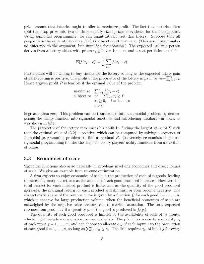
Concave envelope. If we choose fi to be concave, then subproblem (4) is a convex opti-mization problem, and can be solved efficiently (Boyd and Vandenberghe 2004). The tightestconcave approximation to f is obtained by choosing f to be the concave envelope of the func-tion f , which is defined as the pointwise infimum over all concave functions g that are greaterthan or equal to f . For a sigmoidal function, the concave envelope is particularly easy tocalculate. We can write f of f piecewise as

f(x) =

{f(l) + f(w)−f(l)

w−l (x− l) l ≤ x ≤ w

f(x) w ≤ x ≤ u,

15

w

z

Figure 5: The concave envelope f (dashed line) of the logistic function f (solidline).

for some w > z (see Figure 5). The point w can easily be found by bisection: if x < w, thenthe line from (l, f(l) to (x, f(x) crosses the graph of f at x (from lying above the graph tolying below); if x > w, it crosses in the opposite direction.

When we use the concave envelope to compute the bounds (5) and (6), and the constraintset C consists only of m linear equalities and inequalities, Theorem 2 from (Udell and Boyd2014) guarantees that these bounds satisfy

U(Q)− L(Q) ≤min(m,n)∑i=1

ρ[i],

whereρ(f) = sup

x∈Q(f(x)− f(x))

and ρ[i] is defined to be the ith largest of the nonconvexities ρ(f1), . . . , ρ(fn). As the algorithmproceeds, the size of the rectangles decreases, and so U(Q)− L(Q) also decreases.

Piecewise linear upper bound. When all the constraints are linear, it may be convenientto construct a piecewise linear concave upper bound on the function f , and to maximize thispiecewise linear upper bound instead of the concave envelope (see Figure 6). In this case, ifC is a polyhedron, the computation of upper and lower bounds on p?(Q) reduces to a linearprogramming problem (Boyd and Vandenberghe 2004).

If f is differentiable, a piecewise linear concave upper bound, f , may be constructed as

f(y) = infx∈S′

f(x) + f ′(x)(y − x)

where S ′ = {w} ∪ S for any S ⊆ [w,∞). Since the maximum error f(x) − f(x) in theapproximation must occur where adjacent lines intersect, the points of intersection may be

16

added to the set S ′ until the maximum error is less than ε, producing an upper bound thatsatisfies supx f(x)− f(x) ≤ ε.

If f is not differentiable, define f ′(w) = f(w)−f(l)w−l , and let f ′(x) be any supergradient of

f at x for x > w. (A supergradient g of f at x satisfies f(y) ≤ f(x) + g(y − x) for anyy ∈ [z,∞).)

Figure 6: A piecewise linear approximation (dashed line) to the concave envelopeof the (solid line) logistic function.

This approach to solving subproblem (4) has the advantage that it requires minimalinformation about the functions fi: we need only know

1. an oracle for computing the value of the function at a point,

2. an oracle for computing a supergradient of the function at a point, and

3. the value zi (so that we can compute wi).

(As mentioned above, zi can also be easily computed by bisection as a preprocessing step.)In particular, this means that a solver using this approach to solve subproblem (4) need notknow the full functional form of the functions fi. Hence users can add their own customsigmoidal functions fi with relative ease.

Cutting plane upper bound. A cutting plane method may also be used to solve subprob-lem (4). This approach is similar to the method described above for computing a piecewiselinear concave upper bound, but has the advantage that not all pieces of the piecewise linearupper bound need be constructed.

For each function fi in the sum, introduce an epigraph variable ti. Instead of maximizing∑ni=1 fi(xi), we shall maximize

∑ni=1 ti, and add as many linear constraints as are necessary

to ensure that ti ≤ fi(xi) at the solution (x, t). For each i = 1, . . . n, we begin with just twoconstraints on each epigraph variable t:

t ≤ f ′i(wi)(x− wi) + fi(wi) ti ≤ f ′i(ui)(x− ui) + fi(ui),

17

and add more as needed. (This notation assumes that fi is differentiable. If it is not, then

define f ′i(wi) = fi(wi)−fi(li)wi−li , and let f ′i(x) be any supergradient of fi at x for x > wi. We will

not need to invoke f ′i(x) for any x < wi.)More formally, start by setting Ci = {wi, ui}, and solve the problem

maximize∑n

i=1 tisubject to ti ≤ f ′i(y)(xi − y) + fi(y), y ∈ Ci.

(7)

Now using the solution (x, t) to this problem, for each i = 1, . . . n, check if ti > fi(xi) and ifso, update Ci = Ci ∪ {xi}. If any of the sets Ci have changed, solve problem (7) again, andrepeat until the sets Ci do not change.

Alternatively, we may choose to add a new point to Ci only if ti > fi(xi) + ε/n for sometolerance ε. In this case, the algorithm will terminate with

n∑i=1

fi(xi) ≤n∑i=1

ti ≤n∑i=1

fi(xi) + ε,

giving an upper bound∑n

i=1 ti and lower bound∑n

i=1 fi(xi) on the optimal value of prob-lem (4) that differ by no more than ε.

This cutting plane approach can be made particularly fast by using the previous solution(x, t) as a hot-start for problem (7) when new points are added to the sets Ci. This is theapproach adopted to solve the subproblems (4) in the SigmoidalProgramming implementa-tion of this method. Note that the cutting plane approach also requires the same oracle-styleinterface to the functions fi as the piecewise linear upper bound approach.

Branch. The concave envelope of f over the interval (l, u) is equal to f at l and u, andin general will lie closer to f on small intervals, or on intervals over which f is less stronglyconvex (closer to linear). These properties allow us to find tighter bounds on the optimalvalue of the problem over a smaller region than over a larger one, with the size required to finda bound of a given tightness controlled by the convexity of the function. Hence, we branch bysplitting the rectangle with the largest upper bound along the coordinate i with maximumerror εi = fi(x

?i (Q)) − fi(x

?i (Q)) into two subrectangles that meet at min(x?i (Q), zi). The

concave approximation of fi on the subrectangles is then exact at x?i (Q), so that each branchmaximally reduces the error at the previous solution.

Convergence. In Appendix A, we show that the number of concave subproblems thatmust be solved to achieve accuracy εdes is bounded by

n∏i=1

(⌈(hi(zi)− hi(li)) (zi − li)

εdes/n

⌉+ 1

),

where Qinit = (l1, u1)×· · ·× (ln, un), zi = arg max[li,ui] hi(x) for i = 1, . . . , n, and hi : R→ Ris any upper semi-continuous quasi-concave function such that fi(x) =

∫ xlihi(t) dt (which

always exists, if fi is sigmoidal).

18

Pruning. If maxQ∈Q L(Q) > U(Q′), we know with certainty that the solution is not inrectangle Q′, and we may safely delete rectangle Q′ from the set Q. In this case we saythat rectangle Q′ has been pruned. Conversely, we use the notion that a rectangle is activeto mean that the possibility of finding the optimum in that rectangle has not been ruledout. The list of active rectangles maintained by the branch and bound algorithm then hasan interpretation as the set of rectangles in which one is guaranteed to find at least onepoint for which the value of the objective differs from the optimal value by no more thanmaxQ∈Q U(Q)−maxQ∈Q L(Q).

Note that our branching rule makes it unnecessary to explicitly prune the set Q: ifU(Q′) > maxQ∈Q L(Q), then the algorithm will terminate before rectangle Q′ is selected.

6.1 Extensions

Sums of sigmoidal functions. It is worthwhile noting that the algorithm given abovemay be applied to other problem classes. The only requirement of the algorithm is the abilityto construct a concave upper bound on the function to be maximized on any rectangle, whichbecomes provably tight as the size of the rectangle decreases. Hence this algorithm may beapplied not only to sums of sigmoidal functions, but to sums of other functions with otherconvexity properties.

The concave envelope of a function f is, by definition, the smallest concave functionmajorizing f . So we can never arrive at a tighter approximation to f by computing theconcave envelopes of some decomposition of f . That is, for any decomposition f(x) =∑

i gi(x), we have f(x) ≤∑

i gi(x). Hence the upper and lower bounds achieved will betightest when the branch and bound algorithm is applied directly to f , rather than to somedecomposition of f .

This observation has a number of simple consequences. We showed in the introductionthat any univariate function with known regions of convexity and concavity can be writtenas a sum of sigmoidal functions. However, applying this algorithm directly to the originalfunction might result in a more tight concave approximation, and hence faster convergence.Conversely, a difference of convex (DC) programming approach would be to decomposea sigmoidal function into one convex and one concave function, and apply the algorithmdirectly to these. However, the concave envelope of the convex function over the region willnever be tighter than the concave envelope of the sigmoidal function. Hence the algorithmis unlikely to converge more quickly.

Penalty functions. Our method also extends to problems of the form

maximize∑n

i=1 fi(xi) + φ(x)subject to x ∈ C,

where φ is a concave reward function.

19

7 Numerical examples

In this section, we solve a number of sigmoidal programs using SigmoidalProgramming,an implementation written in Julia of the algorithm described in §6. This open sourceimplementation is available online, with documentation, at

https://github.com/madeleineudell/SigmoidalProgramming.jl.

This implementation models the subproblem created at each node in the branch and boundtree using the JuMP optimization modeling library (Lubin and Dunning 2013), making iteasy to substitute different solvers. In the examples below, all the convex subproblems aresimply linear programs. By default, and in the examples below, SigmoidalProgramming

uses GLPK (Makhorin 2006) to solve these LPs.All experiments presented below were conducted on a desktop computer with a 3 GHz

Intel Core 2 Duo processor, running Mac OS X 10.8.

7.1 Bidding example

As our first numerical example we consider an instance of the bidding problem given in §3.2.In Figure 7, results are shown for an example in which

fi(bi) = logistic(αibi + βi)− logistic(βi),

with vi drawn uniformly at random from the interval [0, 4], αi = 10, and βi = −3vi, fori = 1, . . . , n. We set the budget B = .2

∑ni=1 vi. Each graph represents one variable

and its associated objective function (solid line) and concave approximation (dashed line)on the rectangle containing the solution. The solution x?i for each variable is given by thex coordinate of the red X. The rectangle containing the solution is bounded by the solidgrey lines and the endpoints of the interval. For n = 36, the solution even after the firstiteration is quite close to optimality, and the sigmoidal programming algorithm reaches asolution within ε = .01 of optimality after solving only 17 convex subproblems. Noticethat the solution lies along the concave part of the curve, or at the lower bound, for nearlyevery coordinate. This phenomenon illustrates a generic feature of allocation problems: theconvex portion of the curve offers the best “bang-per-buck” (i.e., utility as a function of theresources used), and so the optimal solution generally exploits this region fully or gives upon the coordinate entirely.

Table 1 gives the performance of the algorithm on bidding problems ranging in size nin producing a solution within ε = .01n of the global solution, with the other problemparameters drawn according to the same model as above. The table shows the number ofsubproblems solved and time to achieve a solution. As n increases, the time to solve eachsubproblem increases (since the linear program that we solve at each step is substantiallylarger), but the number of subproblems that must be solved to achieve the same relativeerror decreases, as we expect from the approximation guarantees given in §5.

20

0.00.20.40.60.80.00.10.20.30.4

0.00.51.01.52.00.00.20.40.60.81.01.2

0.00.20.40.60.81.01.21.40.00.10.20.30.40.50.60.7

0.00.51.01.52.02.50.00.20.40.60.81.01.2

0.00.51.01.52.02.50.00.20.40.60.81.01.21.4

0.000.050.100.150.200.250.000.010.020.030.04

0.000.010.020.030.040.050.00000.00050.00100.00150.00200.00250.00300.0035

0.00.51.01.52.02.53.03.50.00.51.01.52.0

0.00.20.40.60.81.00.00.10.20.30.4

0.00.20.40.60.80.00.10.20.30.4

0 1 2 3 40.00.51.01.52.0

0.00.51.01.50.00.20.40.60.81.0

0.00.51.01.52.02.53.03.50.00.51.01.52.0

0.00.51.01.50.00.20.40.60.81.0

0.00.51.01.52.02.50.00.20.40.60.81.01.21.4

0.00.10.20.30.40.50.60.000.050.100.150.20

0.00.51.01.52.02.50.00.20.40.60.81.01.21.4

0.00.51.01.52.02.53.03.50.00.51.01.52.0

0.00.51.01.52.00.00.20.40.60.81.0

0.00.51.01.52.02.53.00.00.51.01.5

0.00.51.01.52.02.50.00.20.40.60.81.01.21.4

0.000.050.100.150.200.250.000.010.020.030.04

0.00.51.01.52.02.53.00.00.51.01.5

0.00.51.01.52.00.00.20.40.60.81.01.2

0.00.20.40.60.81.01.20.00.10.20.30.40.5

0.000.020.040.060.080.100.120.0000.0050.0100.015

0.00.51.01.52.02.53.03.50.00.51.01.52.0

0.00.51.01.50.00.20.40.60.81.0

0.00.51.01.52.02.53.00.00.51.01.5

0.00.51.01.52.02.53.03.50.00.51.01.52.0

0.00.51.01.52.02.50.00.51.01.5

0.00.51.01.52.02.53.03.50.00.51.01.52.0

0.00.51.01.50.00.10.20.30.40.50.60.70.8

0.00.51.01.52.02.53.00.00.51.01.5

0.00.51.01.50.00.20.40.60.8

0.00.51.01.52.02.53.03.50.00.51.01.52.0

Figure 7: Solution for bidding example.

Table 1: Performance on bidding problems.n subproblems time (s)10 12 .1020 28 .1050 46 .39100 1 .01200 1 .03500 1 .091000 1 .302000 1 .955000 1 5.0910000 1 19.73

7.2 Network utility maximization

Our second example demonstrates the speed of the method on a typical allocation typeproblem. We consider the network utility maximization problem previously introduced in§3.4,

maximize∑n

i=1 fi(xi)subject to Ax ≤ c

x ≥ 0,

where x represent flows, c are edge capacities, A is the edge incidence matrix mapping flowsonto edges, and fi(xi) is the utility derived from flow i.

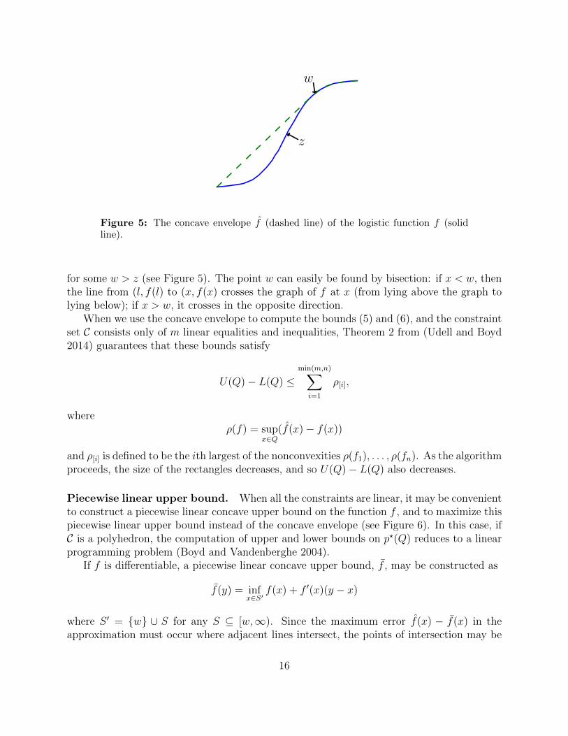
Figure 8 shows the convergence of the algorithm for a network with n = 500 flows over500 edges, with each flow using on average 2.5 edges each, where we use admittance functionsas the utility functions fi, and each edge has capacity 2.5. Within 14 iterations, the solution

21

is within 3% of optimality.

0 2 4 6 8 10 12 14iteration

186

188

190

192

194

196

198

bound

lower boundupper bound

Figure 8: Convergence for NUM with admission function utilities, with n = 500flows over 500 edges, with each flow using on average 2.5 edges each.

7.3 Political marketing example

We now consider an application of the targeted marketing problem (§3.1) to political mar-keting, in which the decision variables correspond to the positions that a politician takes oneach particular issue, and the functions correspond to the expected number of votes for thatpolitician from a given constituency. The goal of the politician is to choose positions on eachissue to maximize his vote share.

The idea that politicians might opportunistically choose their positions in order to maxi-mize their vote share is very old, going back to Downs (1957) and Hotelling (1929), in whichvoters’ preferences are assumed to be distributed in some one-dimensional parameter space.Today, the spatial theory of voting expresses the idea that voters pick candidates based onthe distance in “policy space” between the voter and candidate (Merrill and Grofman 1999).However, this model has generally proven intractable, since the nonconvexity of the politi-cian’s objective leads to a difficult (as we have shown) optimization problem, even with arelatively low-dimensional issue space (Roemer 2006). See, e.g., Adams et al (2005) or Roe-mer (2006, 2004) for more detailed models of party competition based on the spatial theory

22

of voting.

Data. Problem data is generated using responses from the 2008 American National Elec-tion Survey (ANES 2008). Each respondent r in the survey rates each candidate c in the2008 U.S. presidential election as having positions yrc ∈ [1, 7]m on m issues. Respondentsalso say how happy they would be hrc ∈ [1, 7] if the candidate c won. We suppose a respon-dent would vote for a candidate c if hrc > hrc

′for any other candidate c′. If so, vrc = 1 and

otherwise vrc = 0.For each candidate c and state i, we predict that a respondent r ∈ Si in state i will vote

for candidate c with probability logistic((wci )Tyrc), depending on the candidate’s perceived

positions yrc. The parameter vector wci is found by fitting a logistic regression model to theANES data for each candidate and state pair.

Note that the data from the ANES 2008 survey is not meant to be representative of thepopulation of the US on a state by state basis. It includes information on respondents fromonly 34 states, some with only 14 respondents.

Optimizing electoral votes. Suppose each state i has pi votes, which are allocated en-tirely to the winner of the popular vote. Let y ∈ Rm denote the positions the politiciantakes on each of the m issues. The politician’s pandering to state i is given by xi = wTi y.Using our model, the expected number of votes from state i is

fi(xi) = piΦ

(logistic(xi)− .5√

logistic(xi)(1− logistic(xi))/Ni

),

which is sigmoidal in xi, where Φ is the normal CDF and Ni is the number of voters in statei. Hence the politician will win the most votes if y is chosen by solving

maximize∑n

i=1 fi(xi)subject to xi = wTi y, i = 1, . . . , n

1 ≤ y ≤ 7.

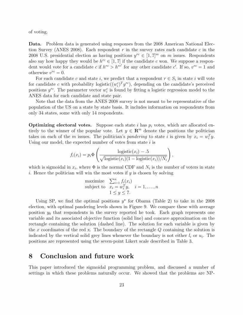
Using SP, we find the optimal positions y? for Obama (Table 2) to take in the 2008election, with optimal pandering levels shown in Figure 9. We compare these with averageposition y0 that respondents in the survey reported he took. Each graph represents onevariable and its associated objective function (solid line) and concave approximation on therectangle containing the solution (dashed line). The solution for each variable is given bythe x coordinates of the red x. The boundary of the rectangle Q containing the solution isindicated by the vertical solid grey lines whenever the boundary is not either li or ui. Thepositions are represented using the seven-point Likert scale described in Table 3.

8 Conclusion and future work

This paper introduced the sigmoidal programming problem, and discussed a number ofsettings in which these problems naturally occur. We showed that the problems are NP-

23

AL AZ CA CO CT

DC DE FL GA IL

IN KS LA MA MI

MN MS NC ND NJ

NM NV NY OH OK

OR PA RI SC TN

TX VA WA WI

Figure 9: Optimal pandering for Obama in 2008.

Table 2: Optimal positions for Obama.Issue y? y0

spending/services 1.26 5.30defense spending 1.27 3.69liberal/conservative 1.00 3.29govt assistance to blacks 1.00 3.12

Table 3: Encoding of positions.Issue 1 7

spending/services fewer services more servicesdefense spending decrease spending increase spendingliberal/conservative liberal conservativegovt assistance govt should help blacks should helpto blacks blacks themselves

hard in general, and even NP-hard to approximate, but that they may be easier in certainsettings; in particular, when the number of constraints is small. We presented a simpleframework for global optimization of sigmoidal programming problems using a branch andbound framework, taking advantage of the simple structure of sigmoidal functions to computeupper and lower bounds on the objective value via convex optimization, and showed that themethod works well in practice, often requiring the solution of a single convex optimizationproblem to achieve satisfactory bounds.

A number of interesting questions remain for future work.

24

Finite convergence. Branch-and-bound algorithms for separable concave minimizationproblems can often be modified to converge to exact (rather than ε-approximate) solutions ina finite number of iterations; see, for example, Al-Khayyal and Sherali (2000) or Shectmanand Sahinidis (1998). However, these algorithms (and proofs) rely on the property thatsolutions to the problems they study occur only at extreme points of the feasible set. Incontrast, solutions to sigmoidal programs may occur in the interior. Is it possible to modifythe algorithm presented here to ensure finite convergence?

Tighter convergence bounds. Our convergence proof does not make use of the knownupper bound on the approximation error presented in §5. In fact, Udell and Boyd (2014)also observe that a solution x to the convex subproblem can be chosen such that εi(x) isnonzero for only m coordinates i. This fact can be used along with the same argumentspresented in our convergence analysis to reduce the upper bound on the maximum numberof subproblems to

2n∏i=1

(⌈(hi(zi)− hi(li)) (zi − li)

εdes/m

⌉+ 1

),

for m < n. Can further improvements be made using these approximation error bounds?

Better pruning and splitting rules. Our algorithm always splits the rectangle with thehighest upper bound. Is it possible to achieve better convergence in practice using otherrules to select the next rectangle to split?

A Convergence proof

In this section, we bound the number of convex subproblems that must be computed be-fore obtaining a solution of some specified tolerance to the original sigmoidal programmingproblem (3).

Before beginning the proof, we remind the reader of a few of our definitions. For eachsigmoidal function fi : [li, ui]→ R, we define a bounded upper semi-continuous quasi-concavefunction hi : [li, ui]→ R such that

fi(x) = fi(li) +

∫ x

li

hi(t)dt, i = 1, . . . , n.

(Such a function hi always exists: continuity of fi implies that hi can be chosen to be uppersemi-continuous; Lipshitz continuity of fi implies that hi is bounded; and that fi is convexand then concave implies that hi is quasi-concave.)

We let zi ∈ [li, ui] be a point maximizing hi over the interval [li, ui]. (This is equivalentto saying that fi is convex for x < zi, and concave for x > zi.) We define fi : [li, ui]→ R, asbefore, as the concave envelope of the function fi, so that fi(x) ≥ fi(x) for every x ∈ [li, ui].This envelope defines a unique point

wi = min{x ∈ [zi, ui] | fi(x) = fi(x)}.

25

Furthermore, since fi is sigmoidal,

fi(x) = fi(x), x ∈ [wi, ui].

Note in particular that zi ≤ wi.Recall the operation of the sigmoidal programming algorithm. Let x? = x?(Q) be the

solution to the problemmaximize

∑ni=1 fi(xi)

subject to x ∈ C ∩Q.

So long as the total error is still greater than the desired tolerance εdes,

n∑i=1

fi(x?)− fi(x?) ≥ εdes,

the algorithm proceeds by splitting the rectangle Q in order to attain a better approximationon each of the subrectangles. The rectangle Q is split along the coordinate i with the greatesterror εi = fi(x

?i )− fi(x?i ) into two smaller boxes that meet at min(x?i , zi).

We wish to show that this algorithm will terminate after a finite number of splits.Notice that there can be no error in coordinate i if x?i ≥ wi or if x?i = li, since fi is the

concave envelope of fi. Furthermore, since fi and fi are both Lipshitz continuous, the error inthe approximation is bounded by a constant (depending on hi) times the minimum distanceof x?i to li. We formalize this logic below to show that the size of the rectangles exploredcannot be too small, which bounds the number of rectangles we may have to explore.

Error bounds. We first bound hi above and below on [li, wi]. The maximum of hi, bydefinition, occurs at zi:

maxx∈[li,wi]

hi(x) = hi(zi).

As for the minimum, the function hi is quasi-concave, so its minimum must occur at eitherli or wi. In fact, we can show it occurs at li. Let gi = fi(wi)−fi(li)

wi−li . Note that gi is a

superdifferential of fi at wi, and that gi ≤ hi(wi), since hi has been chosen to be uppersemi-continuous. So for x ∈ [li, zi],

fi(x) = fi(li) + gi(x− li) ≤ fi(li) + hi(wi)(x− li).

On the other hand, fi is convex on [li, zi], so for x ∈ [li, zi],

fi(x) ≥ fi(li) + hi(li)(x− li).

Putting these together, we see

fi(li) + hi(li)(x− li) ≤ fi(x) ≤ fi(x) ≤ fi(li) + hi(wi)(x− li),

sohi(li) ≤ hi(wi).

26

We use these to bound fi below on [li, wi]:

fi(x) = fi(li) +

∫ x

li

hi(t)dt

≥ fi(li) +

(min

s∈(li,zi)hi(s)

)(x− li)

≥ fi(li) + hi(li)(x− li).

Similarly, we bound fi above on [li, wi]:

fi(x) = fi(li) +

∫ wi

lihi(t)dt

wi − li(x− li)

≤ fi(li) +

∫ wi

limaxs∈(li,zi) hi(s)dt

wi − li(x− li)

≤ fi(li) + hi(zi)(x− li).

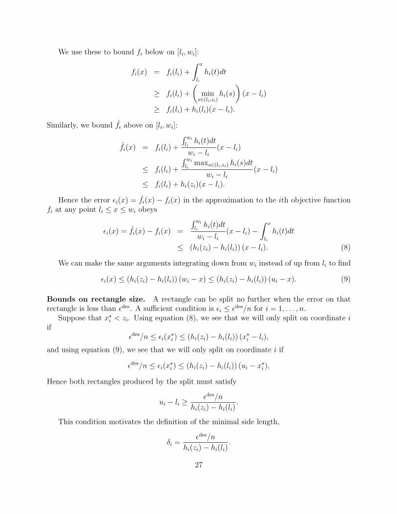
Hence the error εi(x) = fi(x)− fi(x) in the approximation to the ith objective functionfi at any point li ≤ x ≤ wi obeys

εi(x) = fi(x)− fi(x) =

∫ wi

lihi(t)dt

wi − li(x− li)−

∫ x

li

hi(t)dt

≤ (hi(zi)− hi(li)) (x− li). (8)

We can make the same arguments integrating down from wi instead of up from li to find

εi(x) ≤ (hi(zi)− hi(li)) (wi − x) ≤ (hi(zi)− hi(li)) (ui − x). (9)

Bounds on rectangle size. A rectangle can be split no further when the error on thatrectangle is less than εdes. A sufficient condition is εi ≤ εdes/n for i = 1, . . . , n.

Suppose that x?i < zi. Using equation (8), we see that we will only split on coordinate iif

εdes/n ≤ εi(x?i ) ≤ (hi(zi)− hi(li)) (x?i − li),

and using equation (9), we see that we will only split on coordinate i if

εdes/n ≤ εi(x?i ) ≤ (hi(zi)− hi(li)) (ui − x?i ),

Hence both rectangles produced by the split must satisfy

ui − li ≥εdes/n

hi(zi)− hi(li).

This condition motivates the definition of the minimal side length,

δi =εdes/n

hi(zi)− hi(li).

27

The method will never produce a rectangle with a side length smaller than this by splittingat a previous solution, i.e., when x?i < zi.

Conversely, when x?i > zi, the method splits at zi and may produce a left rectangle thatis smaller. But this can only happen at most once for each coordinate.

Formally, we can show

Lemma 1. Every side i of each rectangle produced by the method either contains zi or hasside length at least δi.

Proof. The proof proceeds by induction. It is true for the original rectangle with sides [li, ui].If a rectangle not containing zi is split along coordinate i, then x?i < zi, so the argumentabove shows that both rectangles produced by the split must satisfy ui−li ≥ δi. If a rectanglecontaining zi is split along coordinate i, then either x?i ≥ zi, in which case both rectanglesresulting from the split will contain zi, or x?i < zi, in which case the argument above stillapplies to bound ui − li ≥ δi.

Hence the splits between li and zi along dimension i must be spaced by at least δi fromeach other and from the lower endpoint li.

Bounds on number of convex subproblems. The maximum number of rectangles thatcan fit between li and zi along any dimension i is thus⌈

zi − liδi

⌉,

tiling the interval (li, zi) with rectangles of the minimum allowable side length. And theinterval [zi, ui] can never be split. So the maximal number of rectangles between li and ui is⌈

zi − liδi

⌉+ 1.

This implies the number of leaves l in the tree of rectangles can be at most

l ≤n∏i=1

(⌈zi − liδi

⌉+ 1

).

A binary tree with l leaves has in total 2l − 1 nodes.Hence the number of convex sub-problems solved before the algorithm terminates is bounded by

2l − 1 ≤ 2n∏i=1

(⌈zi − liδi

⌉+ 1

)= 2

n∏i=1

(⌈(hi(zi)− hi(li)) (zi − li)

εdes/n

⌉+ 1

).

In particular, the algorithm converges in a finite number of steps.

28

B Hardness of approximation

In this section, we show there can be no polynomial time algorithm to find an arbitrarilygood approximate solution to any sigmoidal programming (SP) problem unless P=NP. Thusthe algorithm we present for SP, which requires exponential time in some cases to achievea sufficiently good approximate solution, cannot be substantially improved (unless P=NP).The proof uses a reduction of maximum independent set (MIS), a combinatorial optimizationproblem which is known to be NP-hard to approximate on a graph with n vertices withina factor ρ > n1−ε for any ε > 0 (Berman and Schnitger 1992, Hastad 1996, Beigel 1999),to SP. For completeness, we recall that x is an ρ-approximate solution to an maximizationproblem P with objective function F ≥ 0 if x is feasible and

F (x) ≥ ρ−1F (x?),

where x? is the solution to P .The hardness of approximation result relies on a guarantee (proved below) that any non-

integral solution to SP can be rounded to an integral solution with strictly greater objectivefunction, allowing an approximate solution to SP to be used to find an approximate solutionto MIS. For a more thorough discussion of approximation algorithms and techniques forproving hardness of approximation results, we refer the reader to Hochbaum (1996), Vazirani(2001).

Recall the combinatorial optimization problem MIS: given a graph G = (V,E), find amaximal subset of vertices S ⊆ V such that no two vertices in S share an edge. We canwrite the problem as

maximize∑n

i=1 xisubject to xi + xj ≤ 1 (i, j) ∈ E

x ∈ {0, 1}n.(10)

We now describe the reduction of MIS to SP. The objective function in the SP formulationwill include both the MIS objective and a term penalizing deviations from integrality. Letf(x) = |x− 1/2| − 1/2. Consider the problem

maximize γ∑n

i=1 f(xi) +∑n

i=1 xisubject to xi + xj ≤ 1 (i, j) ∈ E

x ∈ {0, 1}n.(11)

The first term in the objective vanishes if the solution x is integral, while the second term isjust the MIS objective. Note that γf(x) + x is a sigmoidal function for any γ ∈ R, so (11)is a sigmoidal programming problem. Define

F (x) = γ

n∑i=1

f(xi) +n∑i=1

xi.

Theorem 2. If γ > 1, then every local solution of (11) is integral, and any feasible pointx ∈ [0, 1]n for (11) can be rounded to a integral feasible point xround ∈ {0, 1}n such thatF (x) < F (xround). Hence, x?, the solution to (11), is integral.

29

Proof. Consider a feasible point x ∈ [0, 1]n for the problem (11) that is not integral, andthe vector xround ∈ {0, 1}n that rounds each nonintegral entry xi to the nearest integer. Wechoose the convention that 1/2 is rounded down to 0, so that xround is also a feasible point.

We wish first to show that F (x) < F (xround). Let δi = |xi − xroundi |, for i = 1, . . . , k. Byrounding xi, we increase f(xi) by an amount δi, while decreasing xi by at most δi. This istrue for every i = 1, . . . , k, so

F (xround)− F (x) ≥ (γ − 1)n∑i=1

δi.

That is, for γ > 1, xround always achieves a larger objective value than x (unless xround = x).This shows that any local solution to the problem (11) will always be integral, and so inparticular the global solution will be integral.

Theorem 2 allows us to show that the optimal value of (11) is equal to the optimal valueof (10). Using the theorem, we know x? ∈ {0, 1}n and f(x?i ) = 0, for i = 1, . . . , n, so theproblem (11) has the same solution and optimal value as

maximize∑n

i=1 xisubject to xi + xj ≤ 1 (i, j) ∈ E

x ∈ {0, 1}n,

which is exactly the MIS problem.This argument shows that sigmoidal programming is NP-hard. We now show it is also

NP-hard to approximate, by using the property, shown above, that the objective value for asolution always increases when the solution is rounded to integrality.

Theorem 3. It is NP-hard to compute an ρ-approximate solution to the sigmoidal program-ming problem

maximize∑n

i=1 fi(xi)subject to x ∈ C,

where fi(x) is sigmoidal i = 1, . . . , n, for ρ > n1−ε with any ε > 0.

Proof. We prove this result by showing that an ρ-approximate solution to the sigmoidalprogramming problem gives a polynomial time computable ρ-approximate solution to MIS.

Let x? be the solution to (11), and consider an ρ-approximate solution xapx to (11) withF (xapx) ≥ ρ−1F (x?) for some ρ ∈ (0, 1). Let xround denote the solution obtained by roundingthe entries of xapx. Then xround still satisfies the constraints of (11), and F (xround) ≥ F (xapx)by theorem (2) if we choose γ > 1. Thus xround is an ρ-approximate solution to (11), sinceF (xround) ≥ F (xapx) ≥ ρ−1F (x?). But notice that xround also satisfies the constraints of (10).That is, xround gives an independent set of size F (xround). Then since the optimal values andsolutions to (10) and (11) are equal,

n∑i=1

xroundi = F (xround) ≥ F (xapx) ≥ ρ−1F (x?) = ρ−1n∑i=1

x?i ,

30

so xround is an ρ-approximate solution to (10).That is, we may use our ρ-approximate solution xapx to (11) to compute in polynomial

time an ρ-approximate solution xround to (10), which is known to be NP-hard for ρ > n1−ε

with any ε > 0 (Berman and Schnitger 1992, Hastad 1996, Beigel 1999).

This theorem shows that there can be no polynomial time approximation scheme (PTAS)for sigmoidal programming, because it is NP-hard to approximate SP to within a factor betterthan n1−ε.

C Acknowledgements

The authors are grateful to Jon Lee, Ernest Ryu, and to a number of anonymous reviewersfor their helpful comments and suggestions. This work was supported by National ScienceFoundation Graduate Research Fellowship program (under Grant No. DGE-1147470), theGabilan Stanford Graduate Fellowship, the Gerald J. Lieberman Fellowship, and the DARPAX-DATA program.

References

Achterberg T (2009) SCIP: solving constraint integer programs. Mathematical Programming Com-putation 1(1):1–41

Adams J, Merrill III S, Grofman B (2005) A unified theory of party competition: a cross-nationalanalysis integrating spatial and behavioral factors. Cambridge University Press

Al-Khayyal F, Sherali H (2000) On finitely terminating branch-and-bound algorithms for someglobal optimization problems. SIAM Journal on Optimization 10(4):1049–1057

Andersen M, Dahl J, Vandenberghe L (2013) CVXOPT: A Python package for convex optimiza-tion, version 1.1.5. URL abel.ee.ucla.edu/cvxopt

ANES (2008) The ANES 2008 time series study dataset. www.electionstudies.org

Balakrishnan V, Boyd S, Balemi S (1991) Branch and bound algorithm for computing the minimumstability degree of parameter-dependent linear systems. International Journal of Robust andNonlinear Control 1(4):295–317, DOI 10.1002/rnc.4590010404

Balas E (1968) A note on the branch-and-bound principle. Operations Research 16(2):442–445

Beigel R (1999) Finding maximum independent sets in sparse and general graphs. In: Proceedingsof the tenth annual ACM-SIAM symposium on Discrete algorithms, Society for Industrial andApplied Mathematics, pp 856–857

Belotti P (2009) CoUEnnE: a users manual. Technical Report

Berman P, Schnitger G (1992) On the complexity of approximating the independent set problem.Information and Computation 96(1):77–94

Boyd S, Vandenberghe L (2004) Convex Optimization. Cambridge University Press

Cybenko G (1989) Approximation by superpositions of a sigmoidal function. Mathematics of Con-trol, Signals, and Systems (MCSS) 2:303–314, 10.1007/BF02551274

31

D’Ambrosio C, Lee J, Wachter A (2012) An algorithmic framework for MINLP with separablenon-convexity. In: Mixed Integer Nonlinear Programming, Springer, pp 315–347

Downs A (1957) An economic theory of political action in a democracy. Journal of Political Economy65(2):135–150

Falk J, Soland R (1969) An algorithm for separable nonconvex programming problems. ManagementScience 15(9):550–569

Fazel M, Chiang M (2005) Network utility maximization with nonconcave utilities using sum-of-squares method. In: 44th IEEE Conference on Decision and Control, pp 1867 – 1874,DOI 10.1109/CDC.2005.1582432

Friedman M, Savage L (1948) The utility analysis of choices involving risk. The Journal of PoliticalEconomy 56(4):279–304

Hastad J (1996) Clique is hard to approximate within n1−ε. In: Foundations of Computer Science,1996. Proceedings., 37th Annual Symposium on, IEEE, pp 627–636

Henrion D, Lasserre JB (2005) Detecting global optimality and extracting solutions in gloptipoly.In: Henrion D, Garulli A (eds) Positive Polynomials in Control, Lecture Notes in Control andInformation Science, vol 312, Springer Berlin Heidelberg, pp 293–310, DOI 10.1007/10997703\X

Hochbaum D (1996) Approximation algorithms for NP-hard problems. PWS Publishing Co.

Horst R, Pardalos P, Van Thoai N (2000) Introduction to global optimization. Kluwer AcademicPublishers

Hotelling H (1929) Stability in competition. The Economic Journal 39(153):pp. 41–57

Kahneman D, Tversky A (1979) Prospect theory: An analysis of decision under risk. Econometrica:Journal of the Econometric Society pp 263–291

Karp R (1972) Reducibility among combinatorial problems. Springer

Lasserre J (2001) Global optimization with polynomials and the problem of moments. SIAM Journalon Optimization 11:796–817

Lawler E, Wood D (1966) Branch-and-bound methods: A survey. Operations Research 14(4):699–719

Lipp T, Boyd S (2014) Variations and extensions of the convex-concave procedure

Lubin M, Dunning I (2013) Computing in operations research using Julia. arXiv preprintarXiv:13121431

Makhorin A (2006) GLPK (GNU linear programming kit)

McCormick G (1976) Computability of global solutions to factorable nonconvex programs: Part i:Convex underestimating problems. Mathematical programming 10(1):147–175

Merrill S, Grofman B (1999) A Unified Theory of Voting: Directional and Proximity Spatial Models.Cambridge University Press

Misener R, Floudas C (2014) ANTIGONE: algorithms for continuous/integer global optimizationof nonlinear equations. Journal of Global Optimization 59(2-3):503–526

Parrilo P (2003) Semidefinite programming relaxations for semialgebraic problems. Mathematicalprogramming 96(2):293–320

Roemer J (2004) Modeling party competition in general elections. Cowles Foundation DiscussionPaper

32

Roemer J (2006) Political competition: Theory and applications. Harvard University Press

Sahinidis N (2014) BARON 14.3.1: Global Optimization of Mixed-Integer Nonlinear Programs,User’s Manual

Shectman J, Sahinidis N (1998) A finite algorithm for global minimization of separable concaveprograms. Journal of Global Optimization 12(1):1–36

Sturm J (1999) Using SeDuMi 1.02, a MATLAB toolbox for optimization over symmetric cones.Optimization methods and software 11(1-4):625–653

Tawarmalani M, Sahinidis N (2002) Convexification and global optimization in continuous andmixed-integer nonlinear programming: theory, algorithms, software, and applications, vol 65.Springer Science & Business Media

Tawarmalani M, Sahinidis N (2005) A polyhedral branch-and-cut approach to global optimization.Mathematical Programming 103:225–249

Toh KC, Todd M, Tutuncu R (1999) SDPT3 — a MATLAB software package for semidefiniteprogramming, version 1.3. Optimization Methods and Software 11(1-4):545–581

Tversky A, Kahneman D (1992) Advances in prospect theory: Cumulative representation of un-certainty. Journal of Risk and uncertainty 5(4):297–323

Udell M, Boyd S (2014) Bounding duality gap for separable functions. arXiv preprintarXiv:14104158 1410.4158

Vazirani V (2001) Approximation algorithms. Springer-Verlag New York, Inc., New York, NY, USA

33