maxwell’s equationsand the p electromagnetism
TRANSCRIPT
“fm” — 2007/12/27 — 12:39 — page i — #1
MAXWELL’S EQUATIONS ANDTHE PRINCIPLES OF
ELECTROMAGNETISM
“fm” — 2007/12/27 — 12:39 — page ii — #2
LICENSE, DISCLAIMER OF LIABILITY, AND LIMITED WARRANTY
By purchasing or using this book (the “Work”), you agree that this license grantspermission to use the contents contained herein, but does not give you the right ofownership to any of the textual content in the book or ownership to any of theinformation or products contained in it. This license does not permit use of the Workon the Internet or on a network (of any kind) without the written consent of thePublisher. Use of any third party code contained herein is limited to and subject tolicensing terms for the respective products, and permission must be obtained from thePublisher or the owner of the source code in order to reproduce or network anyportion of the textual material (in any media) that is contained in the Work.
INFINITY SCIENCE PRESS LLC (“ISP” or “the Publisher”) and anyone involved inthe creation, writing, or production of the accompanying algorithms, code, orcomputer programs (“the software”), and any accompanying Web site or software ofthe Work, cannot and do not warrant the performance or results that might be obtainedby using the contents of the Work. The authors, developers, and the Publisher haveused their best efforts to insure the accuracy and functionality of the textual materialand/or programs contained in this package; we, however, make no warranty of anykind, express or implied, regarding the performance of these contents or programs.The Work is sold “as is” without warranty (except for defective materials used inmanufacturing the book or due to faulty workmanship);
The authors, developers, and the publisher of any accompanying content, and anyoneinvolved in the composition, production, and manufacturing of this work will not beliable for damages of any kind arising out of the use of (or the inability to use) thealgorithms, source code, computer programs, or textual material contained in thispublication. This includes, but is not limited to, loss of revenue or profit, or otherincidental, physical, or consequential damages arising out of the use of this Work.
The sole remedy in the event of a claim of any kind is expressly limited toreplacement of the book, and only at the discretion of the Publisher.
The use of “implied warranty” and certain “exclusions” vary from state to state, andmight not apply to the purchaser of this product.
“fm” — 2007/12/27 — 12:39 — page iii — #3
MAXWELL’S EQUATIONS ANDTHE PRINCIPLES OF
ELECTROMAGNETISM
RICHARD FITZPATRICK, PH.D.University of Texas at Austin
Infinity Science Press LLCHingham, Massachusetts
New Delhi
“fm” — 2007/12/27 — 12:39 — page iv — #4
Copyright 2008 by Infinity Science Press LLCAll rights reserved.
This publication, portions of it, or any accompanying software may not be reproduced in any way, stored in a retrievalsystem of any type, or transmitted by any means or media, electronic or mechanical, including, but not limited to,photocopy, recording, Internet postings or scanning, without prior permission in writing from the publisher.
Publisher: David Pallai
INFINITY SCIENCE PRESS LLC11 Leavitt StreetHingham, MA 02043Tel. 877-266-5796 (toll free)Fax 781-740-1677info@infinitysciencepress.comwww.infinitysciencepress.com
This book is printed on acid-free paper.
Richard Fitzpatrick. Maxwell’s Equations and the Principles of Electromagnetism.ISBN: 978-1-934015-20-9
The publisher recognizes and respects all marks used by companies, manufacturers, and developers as a means todistinguish their products. All brand names and product names mentioned in this book are trademarks or service marksof their respective companies. Any omission or misuse (of any kind) of service marks or trademarks, etc. is not anattempt to infringe on the property of others.
Library of Congress Cataloging-in-Publication Data
Fitzpatrick, Richard.Maxwell’s equations and the principles of electromagnetism / Richard Fitzpatrick.
p. cm.Includes bibliographical references and index.ISBN-13: 978-1-934015-20-9 (hardcover with cd-rom : alk. paper)1. Maxwell equations. 2. Electromagnetic theory. I. Title.QC670.F545 2008530.14′1–dc22
2007050220
Printed in the United States of America08 09 10 5 4 3 2 1
Our titles are available for adoption, license or bulk purchase by institutions, corporations, etc. For additionalinformation, please contact the Customer Service Dept. at 877-266-5796 (toll free).
Requests for replacement of a defective CD-ROM must be accompanied by the original disc, your mailing address,telephone number, date of purchase and purchase price. Please state the nature of the problem, and send the informationto Infinity Science Press, 11 Leavitt Street, Hingham, MA 02043.
The sole obligation of Infinity Science Press to the purchaser is to replace the disc, based on defective materials or faultyworkmanship, but not based on the operation or functionality of the product.

“fm” — 2007/12/27 — 12:39 — page v — #5
For Faith

“fm” — 2007/12/27 — 12:39 — page vi — #6
“fm” — 2007/12/27 — 12:39 — page vii — #7
CONTENTS
Chapter 1. Introduction 1
Chapter 2. Vectors and Vector Fields 5
2.1 Introduction 52.2 Vector Algebra 52.3 Vector Areas 82.4 The Scalar Product 102.5 The Vector Product 122.6 Rotation 152.7 The Scalar Triple Product 172.8 The Vector Triple Product 182.9 Vector Calculus 192.10 Line Integrals 202.11 Vector Line Integrals 232.12 Surface Integrals 242.13 Vector Surface Integrals 262.14 Volume Integrals 272.15 Gradient 282.16 Divergence 322.17 The Laplacian 362.18 Curl 382.19 Polar Coordinates 432.20 Exercises 45
Chapter 3. Time-Independent Maxwell Equations 49
3.1 Introduction 493.2 Coulomb’s Law 493.3 The Electric Scalar Potential 543.4 Gauss’ Law 573.5 Poisson’s Equation 663.6 Ampère’s Experiments 68
vii
“fm” — 2007/12/27 — 12:39 — page viii — #8
viii CONTENTS
3.7 The Lorentz Force 713.8 Ampère’s Law 753.9 Magnetic Monopoles? 763.10 Ampère’s Circuital Law 793.11 Helmholtz’s Theorem 863.12 The Magnetic Vector Potential 913.13 The Biot-Savart Law 953.14 Electrostatics aND Magnetostatics 973.15 Exercises 101
Chapter 4. Time-Dependent Maxwell Equations 107
4.1 Introduction 1074.2 Faraday’s Law 1074.3 Electric Scalar Potential? 1124.4 Gauge Transformations 1134.5 The Displacement Current 1164.6 Potential Formulation 1234.7 Electromagnetic Waves 1244.8 Green’s Functions 1324.9 Retarded Potentials 1364.10 Advanced Potentials? 1424.11 Retarded Fields 1454.12 Maxwell’s Equations 1494.13 Exercises 151
Chapter 5. Electrostatic Calculations 157
5.1 Introduction 1575.2 Electrostatic Energy 1575.3 Ohm’s Law 1635.4 Conductors 1655.5 Boundary Conditions on the Electric Field 1715.6 Capacitors 1725.7 Poisson’s Equation 1785.8 The Uniqueness Theorem 1795.9 One-Dimensional Solutions of Poisson’s
Equation 1845.10 The Method of Images 1865.11 Complex Analysis 1955.12 Separation of Variables 2025.13 Exercises 209
“fm” — 2007/12/27 — 12:39 — page ix — #9
CONTENTS ix
Chapter 6. Dielectric and Magnetic Media 215
6.1 Introduction 2156.2 Polarization 2156.3 Electric Susceptibility and Permittivity 2176.4 Boundary Conditions For E and D 2186.5 Boundary Value Problems with Dielectrics 2206.6 Energy Density within a Dielectric Medium 2266.7 Force Density within a Dielectric Medium 2286.8 The Clausius-Mossotti Relation 2306.9 Dielectric Liquids in Electrostatic Fields 2336.10 Polarization Current 2376.11 Magnetization 2376.12 Magnetic Susceptibility and Permeability 2406.13 Ferromagnetism 2416.14 Boundary Conditions for B and H 2436.15 Boundary Value Problems with Ferromagnets 2446.16 Magnetic Energy 2496.17 Exercises 251
Chapter 7. Magnetic Induction 255
7.1 Introduction 2557.2 Inductance 2557.3 Self-Inductance 2577.4 Mutual Inductance 2617.5 Magnetic Energy 2647.6 Alternating Current Circuits 2707.7 Transmission Lines 2747.8 Exercises 280
Chapter 8. Electromagnetic Energy and Momentum 283
8.1 Introduction 2838.2 Energy Conservation 2838.3 Electromagnetic Momentum 2878.4 Momentum Conservation 2918.5 Angular Momentum Conservation 2948.6 Exercises 297
Chapter 9. Electromagnetic Radiation 299
9.1 Introduction 2999.2 The Hertzian Dipole 299

“fm” — 2007/12/27 — 12:39 — page x — #10
x CONTENTS
9.3 Electric Dipole Radiation 3069.4 Thompson Scattering 3079.5 Rayleigh Scattering 3109.6 Propagation in a Dielectric Medium 3129.7 Dielectric Constant of a Gaseous Medium 3139.8 Dispersion Relation of a Plasma 3149.9 Faraday Rotation 3189.10 Propagation in a Conductor 3229.11 Dispersion Relation of a Collisional Plasma 3249.12 Normal Reflection at a Dielectric Boundary 3269.13 Oblique Reflection at a Dielectric Boundary 3309.14 Total Internal Reflection 3369.15 Optical Coatings 3399.16 Reflection at a Metallic Boundary 3429.17 Wave-Guides 3439.18 Exercises 348
Chapter 10.Relativity and Electromagnetism 351
10.1 Introduction 35110.2 The Relativity Principle 35110.3 The Lorentz Transformation 35210.4 Transformation of Velocities 35710.5 Tensors 35910.6 Physical Significance of Tensors 36410.7 Space-Time 36510.8 Proper Time 37010.9 4-Velocity and 4-Acceleration 37110.10 The Current Density 4-Vector 37210.11 The Potential 4-Vector 37410.12 Gauge Invariance 37410.13 Retarded Potentials 37510.14 Tensors and Pseudo-Tensors 37710.15 The Electromagnetic Field Tensor 38110.16 The Dual Electromagnetic Field Tensor 38410.17 Transformation of Fields 38610.18 Potential Due to a Moving Charge 38710.19 Field Due to a Moving Charge 38810.20 Relativistic Particle Dynamics 39110.21 Force on a Moving Charge 39310.22 The Electromagnetic Energy Tensor 39410.23 Accelerated Charges 397
“fm” — 2007/12/27 — 12:39 — page xi — #11
CONTENTS xi
10.24 The Larmor Formula 40210.25 Radiation Losses 40610.26 Angular Distribution of Radiation 40710.27 Synchrotron Radiation 40910.28 Exercises 412
Appendix A. Physical Constants 417
Appendix B. Useful Vector Identities 419
Appendix C. Gaussian Units 421
Appendix D. Further Reading 425
Index 427

“fm” — 2007/12/27 — 12:39 — page xii — #12

“chapter1” — 2007/12/14 — 11:35 — page 1 — #1
C h a p t e r 1 INTRODUCTION
The main topic of this book is Maxwell’s Equations. These are a set ofeight, scalar, first-order partial differential equations which constitute acomplete description of classical electric and magnetic phenomena. Tobe more exact, Maxwell’s equations constitute a complete description ofthe classical behavior of electric and magnetic fields.
Electric and magnetic fields were first introduced into electromag-netic theory merely as mathematical constructs designed to facilitate thecalculation of the forces exerted between electric charges and betweencurrent carrying wires. However, physicists soon came to realize thatthe physical existence of these fields is key to making Classical Elec-tromagnetism consistent with Einstein’s Special Theory of Relativity. Infact, Classical Electromagnetism was the first example of a so-calledfield theory to be discovered in Physics. Other, subsequently discovered,field theories include General Relativity, Quantum Electrodynamics, andQuantum Chromodynamics.
At any given point in space, an electric or magnetic field possessestwo properties—a magnitude and a direction. In general, these propertiesvary (continuously) from point to point. It is conventional to representsuch a field in terms of its components measured with respect to someconveniently chosen set of Cartesian axes (i.e., the standard x-, y-, andz-axes). Of course, the orientation of these axes is arbitrary. In otherwords, different observers may well choose differently aligned coordi-nate axes to describe the same field. Consequently, the same electricand magnetic fields may have different components according to dif-ferent observers. It can be seen that any description of electric andmagnetic fields is going to depend on two seperate things. Firstly, thenature of the fields themselves, and, secondly, the arbitrary choice of thecoordinate axes with respect to which these fields are measured. Like-wise, Maxwell’s equations—the equations which describe the behaviorof electric and magnetic fields—depend on two separate things. Firstly,the fundamental laws of Physics which govern the behavior of electricand magnetic fields, and, secondly, the arbitrary choice of coordinateaxes. It would be helpful to be able to easily distinguish those elements
1
“chapter1” — 2007/12/14 — 11:35 — page 2 — #2
2 MAXWELL’S EQUATIONS AND THE PRINCIPLES OF ELECTROMAGNETISM
of Maxwell’s equations which depend on Physics from those which onlydepend on coordinates. In fact, this goal can be achieved by employing abranch of mathematics called vector field theory. This formalism enablesMaxwell’s equations to be written in a manner which is completely inde-pendent of the choice of coordinate axes. As an added bonus, Maxwell’sequations look a lot simpler when written in a coordinate-free fashion.Indeed, instead of eight first-order partial differential equations, thereare only four such equations within the context of vector field theory.
Electric and magnetic fields are useful and interesting because theyinteract strongly with ordinary matter. Hence, the primary applicationof Maxwell’s equations is the study of this interaction. In order to facili-tate this study, materials are generally divided into three broad classes:conductors, dielectrics, and magnetic materials. Conductors contain freecharges which drift in response to an applied electric field. Dielectrics aremade up of atoms and molecules which develop electric dipole momentsin the presence of an applied electric field. Finally, magnetic materialsare made up of atoms and molecules which develop magnetic dipolemoments in response to an applied magnetic field. Generally speaking,the interaction of electric and magnetic fields with these three classes ofmaterials is usually investigated in two limits. Firstly, the low-frequencylimit, which is appropriate to the study of the electric and magnetic fieldsfound in conventional electrical circuits. Secondly, the high-frequencylimit, which is appropriate to the study of the electric and magneticfields which occur in electromagnetic waves. In the low-frequency limit,the interaction of a conducting body with electric and magnetic fieldsis conveniently parameterized in terms of its resistance, its capacitance,and its inductance. Resistance measures the resistance of the body to thepassage of electric currents. Capacitance measures its capacity to storecharge. Finally, inductance measures the magnetic field generated bythe body when a current flows through it. Conventional electric circuitsare can be represented as networks of pure resistors, capacitors, andinductors.
This book commences in Chapter 1 with a review of vector field the-ory. In Chapters 2 and 3, vector field theory is employed to transform thefamiliar laws of electromagnetism (i.e., Coulomb’s law, Ampere’s law,Faraday’s law, etc.) into Maxwell’s equations. The general propertiesof these equations and their solutions are then discussed. In particu-lar, it is explained why it is necessary to use fields, rather than forcesalone, to fully describe electric and magnetic phenomena. It is alsodemonstrated that Maxwell’s equations are soluble, and that their solu-tions are unique. In Chapters 4 to 6, Maxwell’s equations are used to
“chapter1” — 2007/12/14 — 11:35 — page 3 — #3
CHAPTER 1 INTRODUCTION 3
investigate the interaction of low-frequency electric and magnetic fieldswith conducting, dielectric, and magnetic media. The related conceptsof resistance, capacitance, and inductance are also examined. The inter-action of high-frequency radiation fields with various different types ofmedia is discussed in Chapter 8. In particular, the emission, absorption,scattering, reflection, and refraction of electromagnetic waves is inves-tigated in detail. Chapter 7 contains a demonstration that Maxwell’sequations conserve both energy and momentum. Finally, in Chapter 9it is shown that Maxwell’s equations are fully consistent with Einstein’sSpecial Theory of Relativity, and can, moreover, be written in a manifestlyLorentz invariant manner. The relativistic form of Maxwell’s equationsis then used to examine radiation by accelerating charges.
This book is primarily intended to accompany a single-semesterupper-division Classical Electromagnetism course for physics majors. Itassumes a knowledge of elementary physics, advanced calculus, par-tial differential equations, vector algebra, vector calculus, and complexanalysis.
Much of the material appearing in this book was gleaned from theexcellent references listed in Appendix D. Furthermore, the contents ofChapter 2 are partly based on my recollection of a series of lectures givenby Dr. Stephen Gull at the University of Cambridge.

“chapter1” — 2007/12/14 — 11:35 — page 4 — #4
“chapter2” — 2007/11/29 — 13:42 — page 5 — #1
C h a p t e r 2 VECTORS ANDVECTOR FIELDS
2.1 INTRODUCTION
This chapter outlines those aspects of vector algebra, vector calculus,and vector field theory which are required to derive and understandMaxwell’s equations.
2.2 VECTOR ALGEBRA
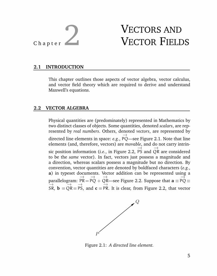
Physical quantities are (predominately) represented in Mathematics bytwo distinct classes of objects. Some quantities, denoted scalars, are rep-resented by real numbers. Others, denoted vectors, are represented by
directed line elements in space: e.g.,→PQ—see Figure 2.1. Note that line
elements (and, therefore, vectors) are movable, and do not carry intrin-
sic position information (i.e., in Figure 2.2,→PS and
→QR are considered
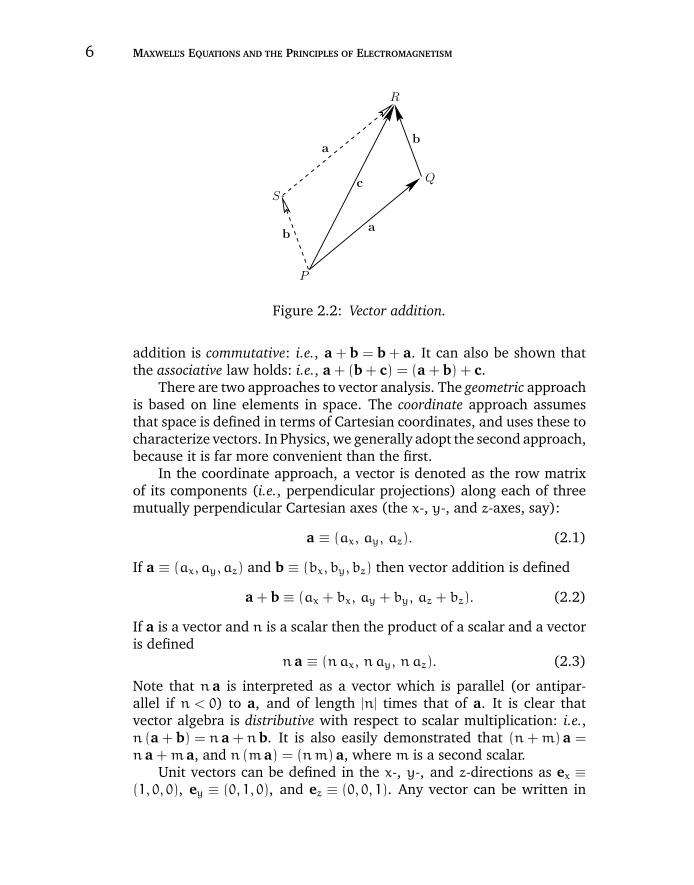
to be the same vector). In fact, vectors just possess a magnitude anda direction, whereas scalars possess a magnitude but no direction. Byconvention, vector quantities are denoted by boldfaced characters (e.g.,a) in typeset documents. Vector addition can be represented using a
parallelogram:→PR=
→PQ +
→QR—see Figure 2.2. Suppose that a ≡
→PQ≡→
SR, b ≡→QR≡
→PS, and c ≡
→PR. It is clear, from Figure 2.2, that vector
P
Q
Figure 2.1: A directed line element.
5
“chapter2” — 2007/11/29 — 13:42 — page 6 — #2
6 MAXWELL’S EQUATIONS AND THE PRINCIPLES OF ELECTROMAGNETISM
c
P
S
R
Q
b
a
a
b
Figure 2.2: Vector addition.
addition is commutative: i.e., a + b = b + a. It can also be shown thatthe associative law holds: i.e., a + (b + c) = (a + b) + c.
There are two approaches to vector analysis. The geometric approachis based on line elements in space. The coordinate approach assumesthat space is defined in terms of Cartesian coordinates, and uses these tocharacterize vectors. In Physics, we generally adopt the second approach,because it is far more convenient than the first.
In the coordinate approach, a vector is denoted as the row matrixof its components (i.e., perpendicular projections) along each of threemutually perpendicular Cartesian axes (the x-, y-, and z-axes, say):
a ≡ (ax, ay, az). (2.1)
If a ≡ (ax, ay, az) and b ≡ (bx, by, bz) then vector addition is defined
a + b ≡ (ax + bx, ay + by, az + bz). (2.2)
If a is a vector and n is a scalar then the product of a scalar and a vectoris defined
n a ≡ (nax, nay, naz). (2.3)
Note that n a is interpreted as a vector which is parallel (or antipar-allel if n < 0) to a, and of length |n| times that of a. It is clear thatvector algebra is distributive with respect to scalar multiplication: i.e.,n (a + b) = n a + nb. It is also easily demonstrated that (n+m) a =n a +m a, and n (m a) = (nm) a, where m is a second scalar.
Unit vectors can be defined in the x-, y-, and z-directions as ex ≡(1, 0, 0), ey ≡ (0, 1, 0), and ez ≡ (0, 0, 1). Any vector can be written in
“chapter2” — 2007/11/29 — 13:42 — page 7 — #3
CHAPTER 2 VECTORS AND VECTOR FIELDS 7
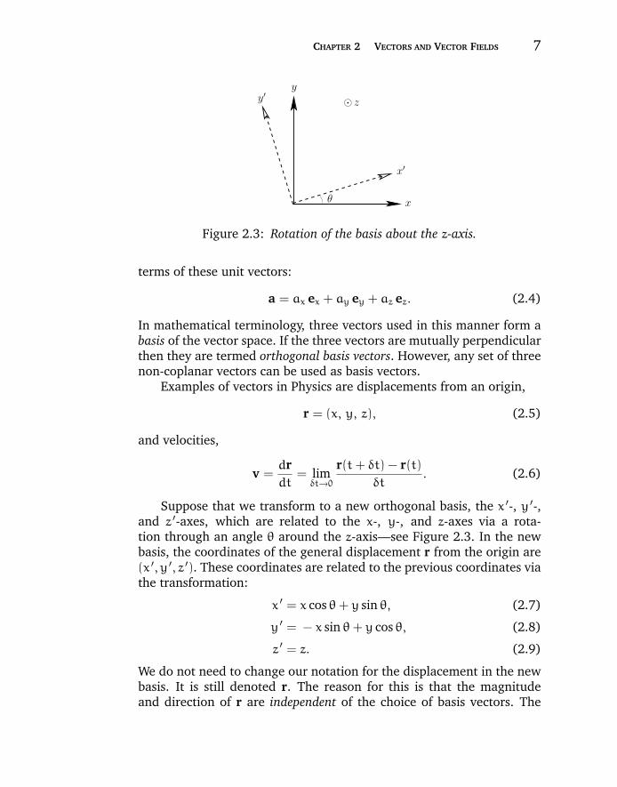
zy′y
x′
xθ
Figure 2.3: Rotation of the basis about the z-axis.
terms of these unit vectors:
a = ax ex + ay ey + az ez. (2.4)
In mathematical terminology, three vectors used in this manner form abasis of the vector space. If the three vectors are mutually perpendicularthen they are termed orthogonal basis vectors. However, any set of threenon-coplanar vectors can be used as basis vectors.
Examples of vectors in Physics are displacements from an origin,
r = (x, y, z), (2.5)
and velocities,
v =drdt
= limδt→0
r(t+ δt) − r(t)δt
. (2.6)
Suppose that we transform to a new orthogonal basis, the x ′-, y ′-,and z ′-axes, which are related to the x-, y-, and z-axes via a rota-tion through an angle θ around the z-axis—see Figure 2.3. In the newbasis, the coordinates of the general displacement r from the origin are(x ′, y ′, z ′). These coordinates are related to the previous coordinates viathe transformation:
x ′ = x cos θ+ y sin θ, (2.7)
y ′ = − x sin θ+ y cos θ, (2.8)
z ′ = z. (2.9)
We do not need to change our notation for the displacement in the newbasis. It is still denoted r. The reason for this is that the magnitudeand direction of r are independent of the choice of basis vectors. The
“chapter2” — 2007/11/29 — 13:42 — page 8 — #4
8 MAXWELL’S EQUATIONS AND THE PRINCIPLES OF ELECTROMAGNETISM
coordinates of r do depend on the choice of basis vectors. However,they must depend in a very specific manner [i.e., Equations (2.7)–(2.9)]which preserves the magnitude and direction of r.
Since any vector can be represented as a displacement from an origin(this is just a special case of a directed line element), it follows thatthe components of a general vector a must transform in an analogousmanner to Equations (2.7)–(2.9). Thus,
ax ′ = ax cos θ+ ay sin θ, (2.10)
ay ′ = − ax sin θ+ ay cos θ, (2.11)
az ′ = az, (2.12)
with analogous transformation rules for rotation about the y- andz-axes. In the coordinate approach, Equations (2.10)–(2.12) constitutethe definition of a vector. The three quantities (ax, ay, az) are the com-ponents of a vector provided that they transform under rotation likeEquations (2.10)–(2.12). Conversely, (ax, ay, az) cannot be the compo-nents of a vector if they do not transform like Equations (2.10)–(2.12).Scalar quantities are invariant under transformation. Thus, the indi-vidual components of a vector (ax, say) are real numbers, but theyare not scalars. Displacement vectors, and all vectors derived from dis-placements, automatically satisfy Equations (2.10)–(2.12). There are,however, other physical quantities which have both magnitude and direc-tion, but which are not obviously related to displacements. We need tocheck carefully to see whether these quantities are vectors.
2.3 VECTOR AREAS
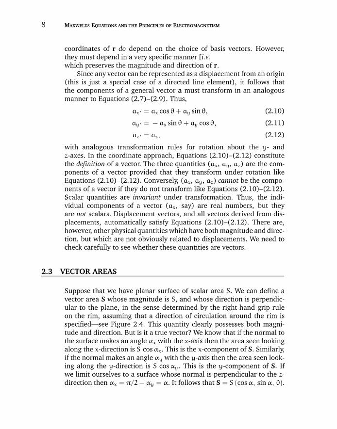
Suppose that we have planar surface of scalar area S. We can define avector area S whose magnitude is S, and whose direction is perpendic-ular to the plane, in the sense determined by the right-hand grip ruleon the rim, assuming that a direction of circulation around the rim isspecified—see Figure 2.4. This quantity clearly possesses both magni-tude and direction. But is it a true vector? We know that if the normal tothe surface makes an angle αx with the x-axis then the area seen lookingalong the x-direction is S cosαx. This is the x-component of S. Similarly,if the normal makes an angle αy with the y-axis then the area seen look-ing along the y-direction is S cosαy. This is the y-component of S. Ifwe limit ourselves to a surface whose normal is perpendicular to the z-direction then αx = π/2− αy = α. It follows that S = S (cosα, sinα, 0).
“chapter2” — 2007/11/29 — 13:42 — page 9 — #5
CHAPTER 2 VECTORS AND VECTOR FIELDS 9
S
Figure 2.4: A vector area.
If we rotate the basis about the z-axis by θ degrees, which is equivalent torotating the normal to the surface about the z-axis by −θ degrees, then
Sx ′ = S cos (α− θ) = S cosα cos θ+ S sinα sin θ = Sx cos θ+ Sy sin θ,(2.13)
which is the correct transformation rule for the x-component of a vector.The other components transform correctly as well. This proves that avector area is a true vector.
According to the vector addition theorem, the projected area of twoplane surfaces, joined together at a line, looking along the x-direction(say) is the x-component of the resultant of the vector areas of the twosurfaces. Likewise, for many joined-up plane areas, the projected area inthe x-direction, which is the same as the projected area of the rim in thex-direction, is the x-component of the resultant of all the vector areas:
S =∑i
Si. (2.14)
If we approach a limit, by letting the number of plane facets increase,and their areas reduce, then we obtain a continuous surface denoted bythe resultant vector area
S =∑i
δSi. (2.15)
It is clear that the projected area of the rim in the x-direction is justSx. Note that the rim of the surface determines the vector area ratherthan the nature of the surface. So, two different surfaces sharing thesame rim both possess the same vector area.
In conclusion, a loop (not all in one plane) has a vector area S whichis the resultant of the vector areas of any surface ending on the loop. The
“chapter2” — 2007/11/29 — 13:42 — page 10 — #6
10 MAXWELL’S EQUATIONS AND THE PRINCIPLES OF ELECTROMAGNETISM
components of S are the projected areas of the loop in the directions ofthe basis vectors. As a corollary, a closed surface has S = 0, since it doesnot possess a rim.
2.4 THE SCALAR PRODUCT
A scalar quantity is invariant under all possible rotational transforma-tions. The individual components of a vector are not scalars becausethey change under transformation. Can we form a scalar out of somecombination of the components of one, or more, vectors? Suppose thatwe were to define the “percent” product,
a % b = ax bz + ay bx + az by = scalar number, (2.16)
for general vectors a and b. Is a % b invariant under transformation, asmust be the case if it is a scalar number? Let us consider an example. Sup-pose that a = (0, 1, 0) and b = (1, 0, 0). It is easily seen that a % b = 1.Let us now rotate the basis through 45 about the z-axis. In the new basis,a = (1/
√2, 1/
√2, 0) and b = (1/
√2, −1/
√2, 0), giving a % b = 1/2.
Clearly, a % b is not invariant under rotational transformation, so theabove definition is a bad one.
Consider, now, the dot product or scalar product:
a · b = ax bx + ay by + az bz = scalar number. (2.17)
Let us rotate the basis though θ degrees about the z-axis. According toEquations (2.10)–(2.12), in the new basis a · b takes the form
a · b = (ax cos θ+ ay sin θ) (bx cos θ+ by sin θ)
+ (−ax sin θ+ ay cos θ) (−bx sin θ+ by cos θ) + az bz
= ax bx + ay by + az bz. (2.18)
Thus, a · b is invariant under rotation about the z-axis. It can eas-ily be shown that it is also invariant under rotation about the x- andy-axes. Clearly, a · b is a true scalar, so the above definition is a goodone. Incidentally, a · b is the only simple combination of the componentsof two vectors which transforms like a scalar. It is easily shown that thedot product is commutative and distributive: i.e.,
a · b = b · a,
a · (b + c) = a · b + a · c. (2.19)
“chapter2” — 2007/11/29 — 13:42 — page 11 — #7
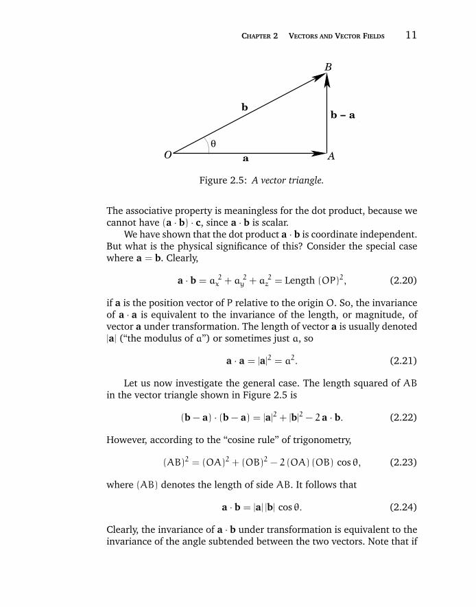
CHAPTER 2 VECTORS AND VECTOR FIELDS 11
b − a
Oθ
A
B
.
b
a
Figure 2.5: A vector triangle.
The associative property is meaningless for the dot product, because wecannot have (a · b) · c, since a · b is scalar.
We have shown that the dot product a · b is coordinate independent.But what is the physical significance of this? Consider the special casewhere a = b. Clearly,
a · b = a 2x + a 2
y + a 2z = Length (OP)2, (2.20)
if a is the position vector of P relative to the origin O. So, the invarianceof a · a is equivalent to the invariance of the length, or magnitude, ofvector a under transformation. The length of vector a is usually denoted|a| (“the modulus of a”) or sometimes just a, so
a · a = |a|2 = a2. (2.21)
Let us now investigate the general case. The length squared of ABin the vector triangle shown in Figure 2.5 is
(b − a) · (b − a) = |a|2 + |b|2 − 2 a · b. (2.22)
However, according to the “cosine rule” of trigonometry,
(AB)2 = (OA)2 + (OB)2 − 2 (OA) (OB) cos θ, (2.23)
where (AB) denotes the length of side AB. It follows that
a · b = |a| |b| cos θ. (2.24)
Clearly, the invariance of a · b under transformation is equivalent to theinvariance of the angle subtended between the two vectors. Note that if
“chapter2” — 2007/11/29 — 13:42 — page 12 — #8
12 MAXWELL’S EQUATIONS AND THE PRINCIPLES OF ELECTROMAGNETISM
a · b = 0 then either |a| = 0, |b| = 0, or the vectors a and b are perpendic-ular. The angle subtended between two vectors can easily be obtainedfrom the dot product:
cos θ =a · b|a| |b|
. (2.25)
The work W performed by a constant force F moving an objectthrough a displacement r is the product of the magnitude of F timesthe displacement in the direction of F. If the angle subtended betweenF and r is θ then
W = |F| (|r| cos θ) = F · r. (2.26)
The rate of flow of liquid of constant velocity v through a loop ofvector area S is the product of the magnitude of the area times thecomponent of the velocity perpendicular to the loop. Thus,
Rate of flow = v · S. (2.27)
2.5 THE VECTOR PRODUCT
We have discovered how to construct a scalar from the components oftwo general vectors a and b. Can we also construct a vector which is notjust a linear combination of a and b? Consider the following definition:
a ∗ b = (ax bx, ay by, az bz). (2.28)
Is a ∗ b a proper vector? Suppose that a = (0, 1, 0), b = (1, 0, 0). Clearly,a ∗ b = 0. However, if we rotate the basis through 45 about thez-axis then a = (1/
√2, 1/
√2, 0), b = (1/
√2, −1/
√2, 0), and a ∗ b =
(1/2, −1/2, 0). Thus, a ∗ b does not transform like a vector, becauseits magnitude depends on the choice of axes. So, the above definition isa bad one.
Consider, now, the cross product or vector product:
a × b = (ay bz − az by, az bx − ax bz, ax by − ay bx) = c. (2.29)
Does this rather unlikely combination transform like a vector? Letus try rotating the basis through θ degrees about the z-axis using
“chapter2” — 2007/11/29 — 13:42 — page 13 — #9
CHAPTER 2 VECTORS AND VECTOR FIELDS 13
Equations (2.10)–(2.12). In the new basis,
cx ′ = (−ax sin θ+ ay cos θ)bz − az (−bx sin θ+ by cos θ)
= (ay bz − az by) cos θ+ (az bx − ax bz) sin θ
= cx cos θ+ cy sin θ. (2.30)
Thus, the x-component of a × b transforms correctly. It can easily beshown that the other components transform correctly as well, and thatall components also transform correctly under rotation about the y- andz-axes. Thus, a × b is a proper vector. Incidentally, a × b is the onlysimple combination of the components of two vectors that transformslike a vector (which is non-coplanar with a and b). The cross product isanticommutative,
a × b = −b × a, (2.31)
distributive,a × (b + c) = a × b + a × c, (2.32)
but is not associative,
a × (b × c) = (a × b) × c. (2.33)
Note that a × b can be written in the convenient, and easy-to-remember,determinant form
a × b =
∣∣∣∣∣∣∣ex ey ezax ay az
bx by bz
∣∣∣∣∣∣∣ . (2.34)
The cross product transforms like a vector, which means that it musthave a well-defined direction and magnitude. We can show that a × b isperpendicular to both a and b. Consider a · a × b. If this is zero then thecross product must be perpendicular to a. Now
a · a × b = ax (ay bz − az by) + ay (az bx − ax bz) + az (ax by − ay bx)
= 0. (2.35)
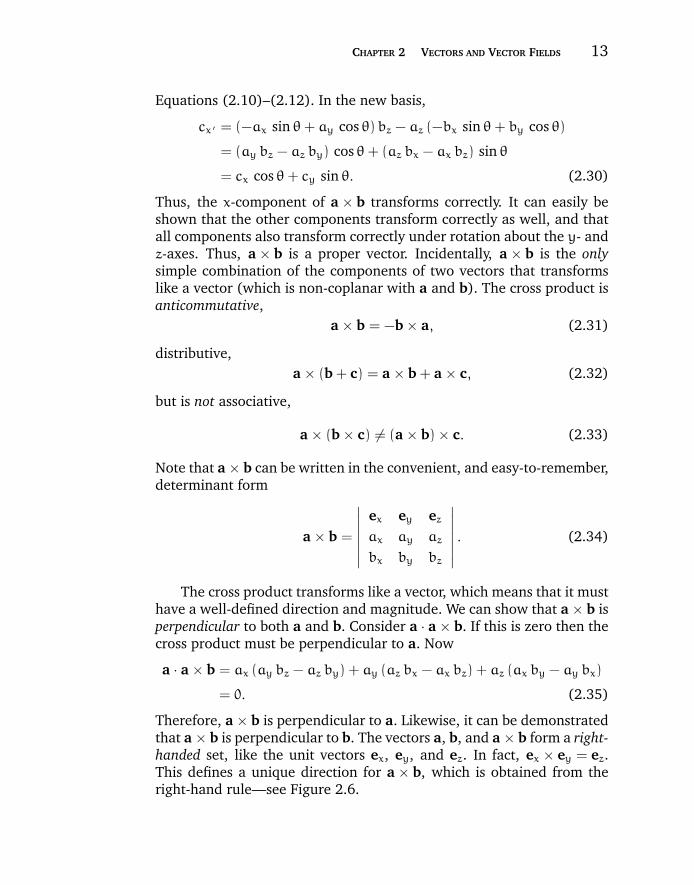
Therefore, a × b is perpendicular to a. Likewise, it can be demonstratedthat a × b is perpendicular to b. The vectors a, b, and a × b form a right-handed set, like the unit vectors ex, ey, and ez. In fact, ex × ey = ez.This defines a unique direction for a × b, which is obtained from theright-hand rule—see Figure 2.6.
“chapter2” — 2007/11/29 — 13:42 — page 14 — #10
14 MAXWELL’S EQUATIONS AND THE PRINCIPLES OF ELECTROMAGNETISM
b
middle finger
index finger
thumb
θ
a × b
a
Figure 2.6: The right-hand rule for cross products. Here, θ is less that 180.
Let us now evaluate the magnitude of a × b. We have
(a × b)2 = (ay bz − az by)2 + (az bx − ax bz)
2 + (ax by − ay bx)2
= (a 2x + a 2
y + a 2z ) (b 2x + b 2y + b 2z ) − (ax bx + ay by + az bz)
2
= |a|2 |b|2 − (a · b)2
= |a|2 |b|2 − |a|2 |b|2 cos2 θ = |a|2 |b|2 sin2 θ. (2.36)
Thus,
|a × b| = |a| |b| sin θ, (2.37)
where θ is the angle subtended between a and b. Clearly, a × a = 0 forany vector, since θ is always zero in this case. Also, if a × b = 0 theneither |a| = 0, |b| = 0, or b is parallel (or antiparallel) to a.
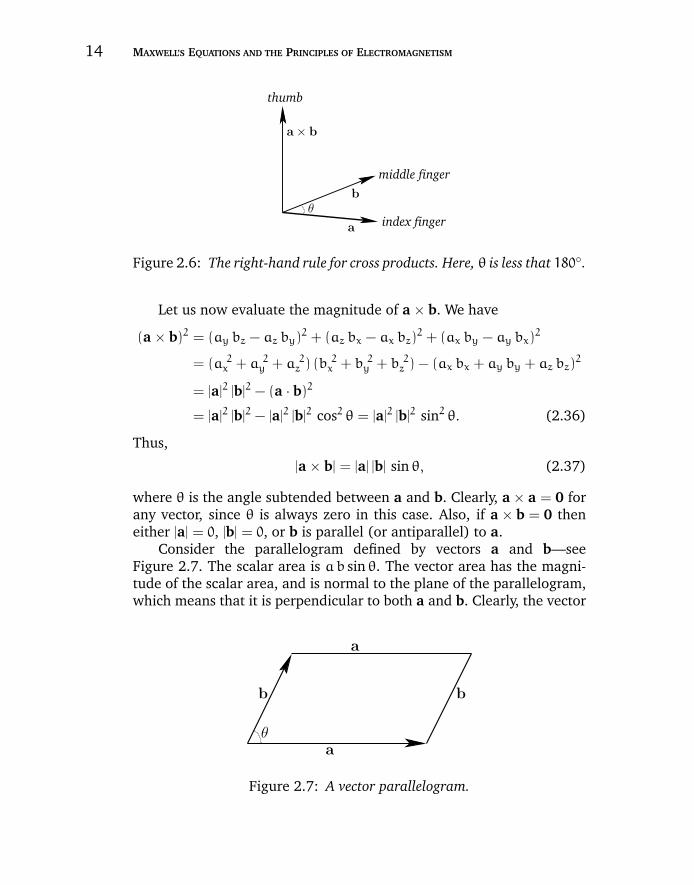
Consider the parallelogram defined by vectors a and b—seeFigure 2.7. The scalar area is ab sin θ. The vector area has the magni-tude of the scalar area, and is normal to the plane of the parallelogram,which means that it is perpendicular to both a and b. Clearly, the vector
b
a
b
θa
Figure 2.7: A vector parallelogram.

“chapter2” — 2007/11/29 — 13:42 — page 15 — #11
CHAPTER 2 VECTORS AND VECTOR FIELDS 15
r
O
θ
P
Q
F
r sin θ
Figure 2.8: A torque.
area is given byS = a × b, (2.38)
with the sense obtained from the right-hand grip rule by rotating aon to b.
Suppose that a force F is applied at position r—see Figure 2.8. Thetorque about the origin O is the product of the magnitude of the forceand the length of the lever arm OQ. Thus, the magnitude of the torqueis |F| |r| sin θ. The direction of the torque is conventionally the directionof the axis throughO about which the force tries to rotate objects, in thesense determined by the right-hand grip rule. It follows that the vectortorque is given by
τ = r × F. (2.39)
2.6 ROTATION
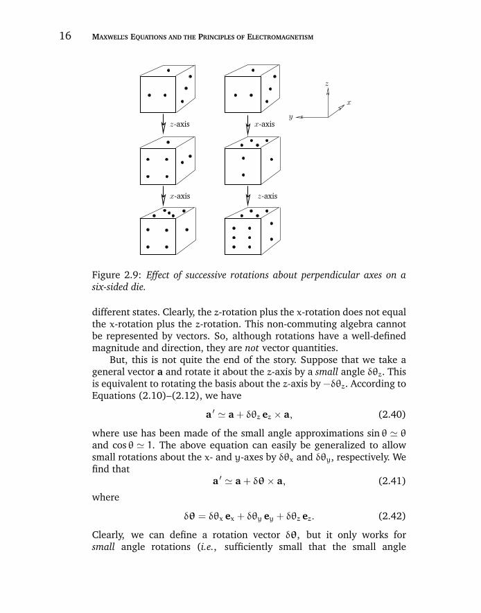
Let us try to define a rotation vector θ whose magnitude is the angleof the rotation, θ, and whose direction is the axis of the rotation, inthe sense determined by the right-hand grip rule. Unfortunately, this isnot a good vector. The problem is that the addition of rotations is notcommutative, whereas vector addition is commuative. Figure 2.9 showsthe effect of applying two successive 90 rotations, one about the x-axis,and the other about the z-axis, to a standard six-sided die. In the left-hand case, the z-rotation is applied before the x-rotation, and vice versa inthe right-hand case. It can be seen that the die ends up in two completely
“chapter2” — 2007/11/29 — 13:42 — page 16 — #12
16 MAXWELL’S EQUATIONS AND THE PRINCIPLES OF ELECTROMAGNETISM
x
x-axisz-axis
x-axis z-axis
z
y
Figure 2.9: Effect of successive rotations about perpendicular axes on asix-sided die.
different states. Clearly, the z-rotation plus the x-rotation does not equalthe x-rotation plus the z-rotation. This non-commuting algebra cannotbe represented by vectors. So, although rotations have a well-definedmagnitude and direction, they are not vector quantities.
But, this is not quite the end of the story. Suppose that we take ageneral vector a and rotate it about the z-axis by a small angle δθz. Thisis equivalent to rotating the basis about the z-axis by −δθz. According toEquations (2.10)–(2.12), we have
a ′ a + δθz ez × a, (2.40)
where use has been made of the small angle approximations sin θ θ
and cos θ 1. The above equation can easily be generalized to allowsmall rotations about the x- and y-axes by δθx and δθy, respectively. Wefind that
a ′ a + δθ × a, (2.41)
where
δθ = δθx ex + δθy ey + δθz ez. (2.42)
Clearly, we can define a rotation vector δθ, but it only works forsmall angle rotations (i.e., sufficiently small that the small angle
“chapter2” — 2007/11/29 — 13:42 — page 17 — #13
CHAPTER 2 VECTORS AND VECTOR FIELDS 17
approximations of sine and cosine are good). According to the aboveequation, a small z-rotation plus a small x-rotation is (approximately)equal to the two rotations applied in the opposite order. The fact thatinfinitesimal rotation is a vector implies that angular velocity,
ω = limδt→0
δθ
δt, (2.43)
must be a vector as well. Also, if a ′ is interpreted as a(t+ δt) in Equa-tion (2.41) then it is clear that the equation of motion of a vectorprecessing about the origin with angular velocity ω is
dadt
= ω × a. (2.44)
2.7 THE SCALAR TRIPLE PRODUCT
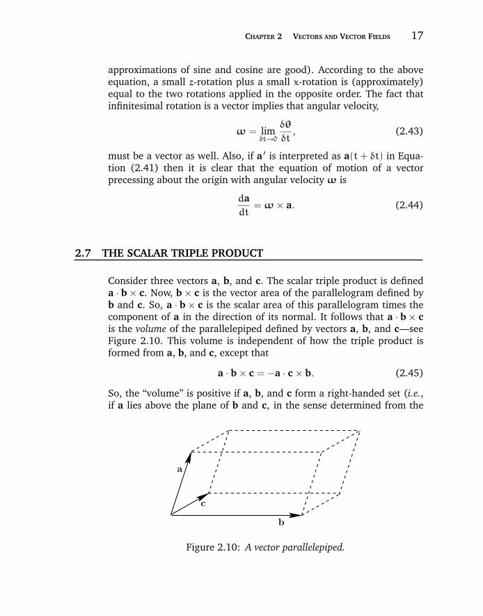
Consider three vectors a, b, and c. The scalar triple product is defineda · b × c. Now, b × c is the vector area of the parallelogram defined byb and c. So, a · b × c is the scalar area of this parallelogram times thecomponent of a in the direction of its normal. It follows that a · b × cis the volume of the parallelepiped defined by vectors a, b, and c—seeFigure 2.10. This volume is independent of how the triple product isformed from a, b, and c, except that
a · b × c = −a · c × b. (2.45)
So, the “volume” is positive if a, b, and c form a right-handed set (i.e.,if a lies above the plane of b and c, in the sense determined from the
c
b
a
Figure 2.10: A vector parallelepiped.
“chapter2” — 2007/11/29 — 13:42 — page 18 — #14
18 MAXWELL’S EQUATIONS AND THE PRINCIPLES OF ELECTROMAGNETISM
right-hand grip rule by rotating b onto c) and negative if they form aleft-handed set. The triple product is unchanged if the dot and crossproduct operators are interchanged,
a · b × c = a × b · c. (2.46)
The triple product is also invariant under any cyclic permutation of a, b,and c,
a · b × c = b · c × a = c · a × b, (2.47)
but any anticyclic permutation causes it to change sign,
a · b × c = −b · a × c. (2.48)
The scalar triple product is zero if any two of a, b, and c are parallel, orif a, b, and c are coplanar.
If a, b, and c are non-coplanar, then any vector r can be written interms of them:
r = α a + βb + γ c. (2.49)
Forming the dot product of this equation with b × c, we then obtain
r · b × c = α a · b × c, (2.50)
so
α =r · b × ca · b × c
. (2.51)
Analogous expressions can be written for β and γ. The parameters α,β, and γ are uniquely determined provided a · b × c = 0: i.e., providedthat the three basis vectors are not coplanar.
2.8 THE VECTOR TRIPLE PRODUCT
For three vectors a, b, and c, the vector triple product is defined a ×(b × c). The brackets are important because a × (b × c) = (a × b) × c.In fact, it can be demonstrated that
a × (b × c) ≡ (a · c) b − (a · b) c (2.52)
and
(a × b) × c ≡ (a · c) b − (b · c) a. (2.53)

“chapter2” — 2007/11/29 — 13:42 — page 19 — #15
CHAPTER 2 VECTORS AND VECTOR FIELDS 19
Let us try to prove the first of the above theorems. The left-handside and the right-hand side are both proper vectors, so if we can provethis result in one particular coordinate system then it must be true ingeneral. Let us take convenient axes such that the x-axis lies along b,and c lies in the x-y plane. It follows that b = (bx, 0, 0), c = (cx, cy, 0),and a = (ax, ay, az). The vector b × c is directed along the z-axis:b × c = (0, 0, bx cy). It follows that a × (b × c) lies in the x-y plane:a × (b × c) = (ay bx cy, −ax bx cy, 0). This is the left-hand side of Equa-tion (2.52) in our convenient axes. To evaluate the right-hand side, weneed a · c = ax cx + ay cy and a · b = ax bx. It follows that the right-handside is
RHS = ( [ax cx + ay cy]bx, 0, 0) − (ax bx cx, ax bx cy, 0)
= (ay cy bx, −ax bx cy, 0) = LHS, (2.54)
which proves the theorem.
2.9 VECTOR CALCULUS
Suppose that vector a varies with time, so that a = a(t). The timederivative of the vector is defined
dadt
= limδt→0
[a(t+ δt) − a(t)
δt
]. (2.55)
When written out in component form this becomes
dadt
=
(dax
dt,day
dt,daz
dt
). (2.56)
Suppose that a is, in fact, the product of a scalar φ(t) and anothervector b(t). What now is the time derivative of a? We have
dax
dt=d
dt(φbx) =
dφ
dtbx + φ
dbx
dt, (2.57)
which implies that
dadt
=dφ
dtb + φ
dbdt. (2.58)
Moreover, it is easily demonstrated that
d
dt(a · b) =
dadt
· b + a · dbdt, (2.59)
“chapter2” — 2007/11/29 — 13:42 — page 20 — #16
20 MAXWELL’S EQUATIONS AND THE PRINCIPLES OF ELECTROMAGNETISM
and
d
dt(a × b) =
dadt
× b + a × dbdt. (2.60)
Hence, it can be seen that the laws of vector differentiation are analogousto those in conventional calculus.
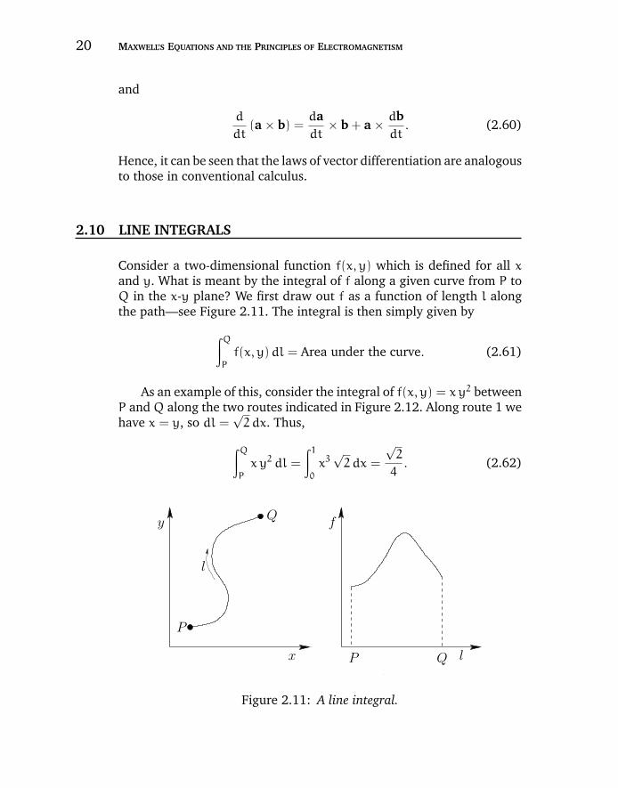
2.10 LINE INTEGRALS
Consider a two-dimensional function f(x, y) which is defined for all xand y. What is meant by the integral of f along a given curve from P toQ in the x-y plane? We first draw out f as a function of length l alongthe path—see Figure 2.11. The integral is then simply given by
∫QP
f(x, y)dl = Area under the curve. (2.61)
As an example of this, consider the integral of f(x, y) = xy2 betweenP andQ along the two routes indicated in Figure 2.12. Along route 1 wehave x = y, so dl =
√2 dx. Thus,
∫QP
xy2 dl =
∫ 10
x3√2 dx =
√2
4. (2.62)
.
lx
y
P
Q
l
P
f
Q
Figure 2.11: A line integral.
“chapter2” — 2007/11/29 — 13:42 — page 21 — #17
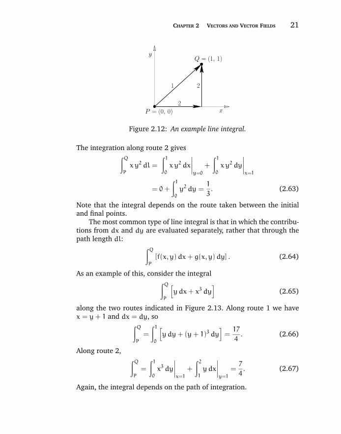
CHAPTER 2 VECTORS AND VECTOR FIELDS 21
y
P = (0, 0)
Q = (1, 1)
1
2
2
x
Figure 2.12: An example line integral.
The integration along route 2 gives∫QP
xy2 dl =
∫ 10
x y2 dx
∣∣∣∣y=0
+
∫ 10
x y2 dy
∣∣∣∣x=1
= 0+
∫ 10
y2 dy =1
3. (2.63)
Note that the integral depends on the route taken between the initialand final points.
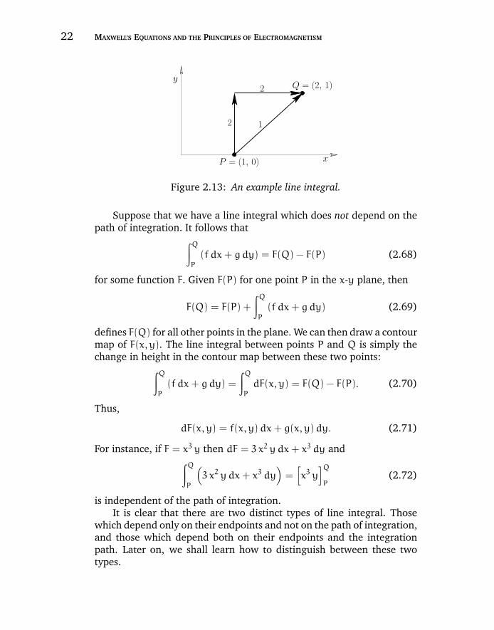
The most common type of line integral is that in which the contribu-tions from dx and dy are evaluated separately, rather that through thepath length dl: ∫Q
P
[f(x, y)dx+ g(x, y)dy] . (2.64)
As an example of this, consider the integral∫QP
[ydx+ x3 dy
](2.65)
along the two routes indicated in Figure 2.13. Along route 1 we havex = y+ 1 and dx = dy, so∫Q
P
=
∫ 10
[ydy+ (y+ 1)3 dy
]=17
4. (2.66)
Along route 2, ∫QP
=
∫ 10
x3 dy
∣∣∣∣x=1
+
∫ 21
y dx
∣∣∣∣y=1
=7
4. (2.67)
Again, the integral depends on the path of integration.
“chapter2” — 2007/11/29 — 13:42 — page 22 — #18
22 MAXWELL’S EQUATIONS AND THE PRINCIPLES OF ELECTROMAGNETISM
2
P = (1, 0)
Q = (2, 1)
1
x
y2
Figure 2.13: An example line integral.
Suppose that we have a line integral which does not depend on thepath of integration. It follows that∫Q
P
(f dx+ gdy) = F(Q) − F(P) (2.68)
for some function F. Given F(P) for one point P in the x-y plane, then
F(Q) = F(P) +
∫QP
(f dx+ gdy) (2.69)
defines F(Q) for all other points in the plane. We can then draw a contourmap of F(x, y). The line integral between points P and Q is simply thechange in height in the contour map between these two points:∫Q
P
(f dx+ gdy) =
∫QP
dF(x, y) = F(Q) − F(P). (2.70)
Thus,
dF(x, y) = f(x, y)dx+ g(x, y)dy. (2.71)
For instance, if F = x3 y then dF = 3 x2 ydx+ x3 dy and∫QP
(3 x2 ydx+ x3 dy
)=[x3 y
]QP
(2.72)
is independent of the path of integration.It is clear that there are two distinct types of line integral. Those
which depend only on their endpoints and not on the path of integration,and those which depend both on their endpoints and the integrationpath. Later on, we shall learn how to distinguish between these twotypes.
“chapter2” — 2007/11/29 — 13:42 — page 23 — #19
CHAPTER 2 VECTORS AND VECTOR FIELDS 23
2.11 VECTOR LINE INTEGRALS
A vector field is defined as a set of vectors associated with each point inspace. For instance, the velocity v(r) in a moving liquid (e.g., a whirlpool)constitutes a vector field. By analogy, a scalar field is a set of scalarsassociated with each point in space. An example of a scalar field is thetemperature distribution T(r) in a furnace.
Consider a general vector field A(r). Let dl = (dx, dy, dz) be thevector element of line length. Vector line integrals often arise as
∫QP
A · dl =
∫QP
(Ax dx+Ay dy+Az dz). (2.73)
For instance, if A is a force field then the line integral is the work donein going from P to Q.
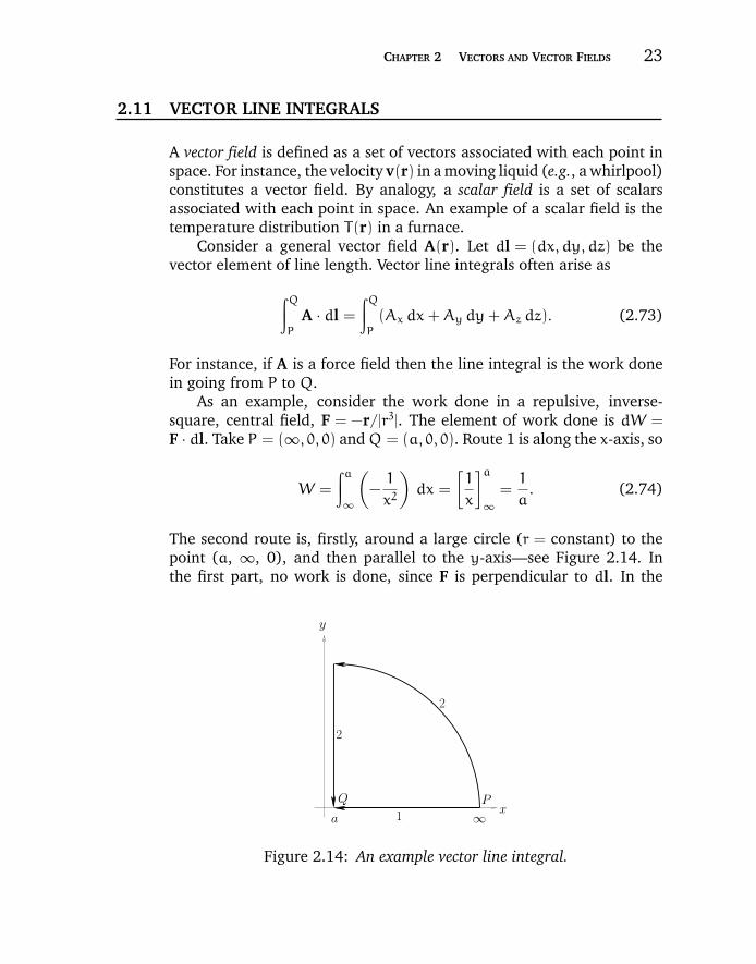
As an example, consider the work done in a repulsive, inverse-square, central field, F = −r/|r3|. The element of work done is dW =F · dl. Take P = (∞, 0, 0) andQ = (a, 0, 0). Route 1 is along the x-axis, so
W =
∫a∞
(−1
x2
)dx =
[1
x
]a∞
=1
a. (2.74)
The second route is, firstly, around a large circle (r = constant) to thepoint (a, ∞, 0), and then parallel to the y-axis—see Figure 2.14. Inthe first part, no work is done, since F is perpendicular to dl. In the
x
2
1
2
Q P
y
a ∞
Figure 2.14: An example vector line integral.
“chapter2” — 2007/11/29 — 13:42 — page 24 — #20
24 MAXWELL’S EQUATIONS AND THE PRINCIPLES OF ELECTROMAGNETISM
second part,
W =
∫ 0∞
−ydy
(a2 + y2)3/2=
[1
(y2 + a2)1/2
]0∞
=1
a. (2.75)
In this case, the integral is independent of the path. However, not allvector line integrals are path independent.
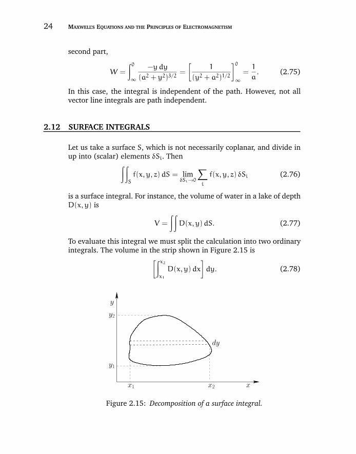
2.12 SURFACE INTEGRALS
Let us take a surface S, which is not necessarily coplanar, and divide inup into (scalar) elements δSi. Then∫∫
S
f(x, y, z)dS = limδSi→0
∑i
f(x, y, z) δSi (2.76)
is a surface integral. For instance, the volume of water in a lake of depthD(x, y) is
V =
∫∫D(x, y)dS. (2.77)
To evaluate this integral we must split the calculation into two ordinaryintegrals. The volume in the strip shown in Figure 2.15 is[∫x2
x1
D(x, y)dx
]dy. (2.78)
dy
x2x1
y1
y2
y
x
Figure 2.15: Decomposition of a surface integral.
“chapter2” — 2007/11/29 — 13:42 — page 25 — #21
CHAPTER 2 VECTORS AND VECTOR FIELDS 25
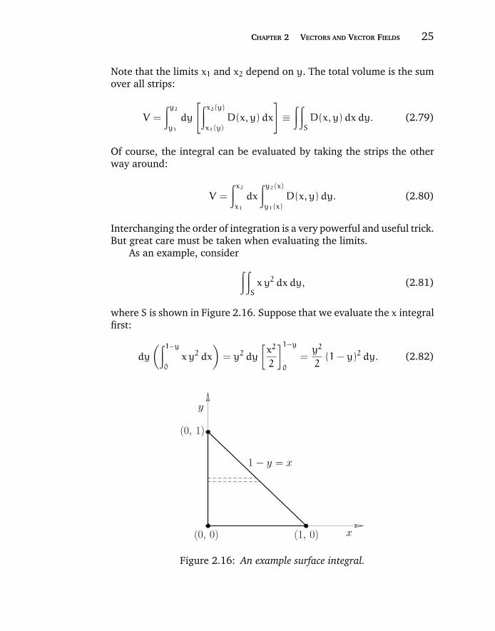
Note that the limits x1 and x2 depend on y. The total volume is the sumover all strips:
V =
∫y2
y1
dy
[∫x2(y)
x1(y)
D(x, y)dx
]≡
∫∫S
D(x, y)dxdy. (2.79)
Of course, the integral can be evaluated by taking the strips the otherway around:
V =
∫x2
x1
dx
∫y2(x)
y1(x)
D(x, y)dy. (2.80)
Interchanging the order of integration is a very powerful and useful trick.But great care must be taken when evaluating the limits.
As an example, consider∫∫S
x y2 dxdy, (2.81)
where S is shown in Figure 2.16. Suppose that we evaluate the x integralfirst:
dy
(∫ 1−y0
x y2 dx
)= y2 dy
[x2
2
]1−y0
=y2
2(1− y)2 dy. (2.82)
1 − y = x
x(1, 0)
(0, 1)
y
(0, 0)
Figure 2.16: An example surface integral.

“chapter2” — 2007/11/29 — 13:42 — page 26 — #22
26 MAXWELL’S EQUATIONS AND THE PRINCIPLES OF ELECTROMAGNETISM
Let us now evaluate the y integral:
∫ 10
(y2
2− y3 +
y4
2
)dy =
1
60. (2.83)
We can also evaluate the integral by interchanging the order ofintegration:
∫ 10
x dx
∫ 1−x0
y2 dy =
∫ 10
x
3(1− x)3 dx =
1
60. (2.84)
In some cases, a surface integral is just the product of two separateintegrals. For instance, ∫ ∫
S
x2 y dxdy (2.85)
where S is a unit square. This integral can be written
∫ 10
dx
∫ 10
x2 y dy =
(∫ 10
x2 dx
)(∫ 10
y dy
)=1
3
1
2=1
6, (2.86)
since the limits are both independent of the other variable.
2.13 VECTOR SURFACE INTEGRALS
Surface integrals often occur during vector analysis. For instance, therate of flow of a liquid of velocity v through an infinitesimal surface ofvector area dS is v · dS. The net rate of flow through a surface S madeup of lots of infinitesimal surfaces is∫∫
S
v · dS = limdS→0
[∑v cos θdS
], (2.87)
where θ is the angle subtended between the normal to the surface andthe flow velocity.
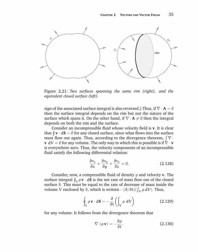
Analogously to line integrals, most surface integrals depend both onthe surface and the rim. But some (very important) integrals dependonly on the rim, and not on the nature of the surface which spans it.As an example of this, consider incompressible fluid flow between twosurfaces S1 and S2 which end on the same rim—see Figure 2.21. The
“chapter2” — 2007/11/29 — 13:42 — page 27 — #23
CHAPTER 2 VECTORS AND VECTOR FIELDS 27
volume between the surfaces is constant, so what goes in must comeout, and ∫∫
S1
v · dS =
∫ ∫S2
v · dS. (2.88)
It follows that ∫∫v · dS (2.89)
depends only on the rim, and not on the form of surfaces S1 and S2.
2.14 VOLUME INTEGRALS
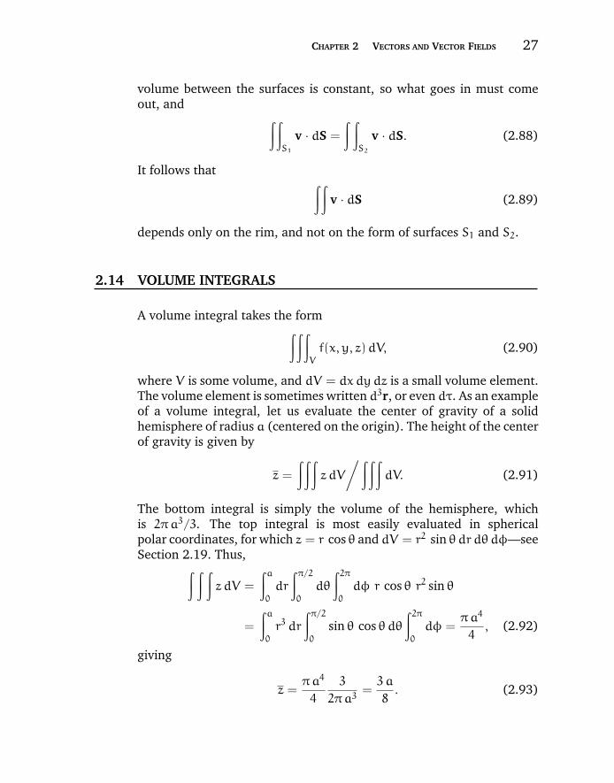
A volume integral takes the form∫∫∫V
f(x, y, z)dV, (2.90)
where V is some volume, and dV = dxdydz is a small volume element.The volume element is sometimes written d3r, or even dτ. As an exampleof a volume integral, let us evaluate the center of gravity of a solidhemisphere of radius a (centered on the origin). The height of the centerof gravity is given by
z =
∫∫∫z dV
/ ∫∫∫dV. (2.91)
The bottom integral is simply the volume of the hemisphere, whichis 2πa3/3. The top integral is most easily evaluated in sphericalpolar coordinates, for which z = r cos θ and dV = r2 sin θdr dθdφ—seeSection 2.19. Thus,∫ ∫ ∫
z dV =
∫a0
dr
∫π/20
dθ
∫ 2π0
dφ r cos θ r2 sin θ
=
∫a0
r3 dr
∫π/20
sin θ cos θdθ∫ 2π0
dφ =πa4
4, (2.92)
giving
z =πa4
4
3
2πa3=3 a
8. (2.93)
“chapter2” — 2007/11/29 — 13:42 — page 28 — #24
28 MAXWELL’S EQUATIONS AND THE PRINCIPLES OF ELECTROMAGNETISM
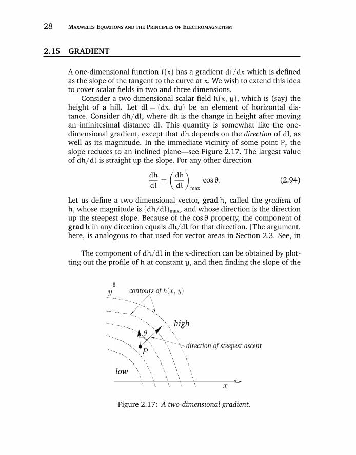
2.15 GRADIENT
A one-dimensional function f(x) has a gradient df/dx which is definedas the slope of the tangent to the curve at x. We wish to extend this ideato cover scalar fields in two and three dimensions.
Consider a two-dimensional scalar field h(x, y), which is (say) theheight of a hill. Let dl = (dx, dy) be an element of horizontal dis-tance. Consider dh/dl, where dh is the change in height after movingan infinitesimal distance dl. This quantity is somewhat like the one-dimensional gradient, except that dh depends on the direction of dl, aswell as its magnitude. In the immediate vicinity of some point P, theslope reduces to an inclined plane—see Figure 2.17. The largest valueof dh/dl is straight up the slope. For any other direction
dh
dl=
(dh
dl
)max
cos θ. (2.94)
Let us define a two-dimensional vector, gradh, called the gradient ofh, whose magnitude is (dh/dl)max, and whose direction is the directionup the steepest slope. Because of the cos θ property, the component ofgradh in any direction equals dh/dl for that direction. [The argument,here, is analogous to that used for vector areas in Section 2.3. See, inparticular, Equation (2.13).]
The component of dh/dl in the x-direction can be obtained by plot-ting out the profile of h at constant y, and then finding the slope of the
direction of steepest ascent
y contours of h(x, y)
θ
x
P
high
low
Figure 2.17: A two-dimensional gradient.
“chapter2” — 2007/11/29 — 13:42 — page 29 — #25
CHAPTER 2 VECTORS AND VECTOR FIELDS 29
tangent to the curve at given x. This quantity is known as the partialderivative of h with respect to x at constant y, and is denoted (∂h/∂x)y.Likewise, the gradient of the profile at constant x is written (∂h/∂y)x.Note that the subscripts denoting constant-x and constant-y are usuallyomitted, unless there is any ambiguity. If follows that in component form
gradh =
(∂h
∂x,∂h
∂y
). (2.95)
Now, the equation of the tangent plane at P = (x0, y0) is
hT (x, y) = h(x0, y0) + α (x− x0) + β (y− y0). (2.96)
This has the same local gradients as h(x, y), so
α =∂h
∂x, β =
∂h
∂y, (2.97)
by differentiation of the above. For small dx = x− x0 and dy = y− y0,the function h is coincident with the tangent plane. We have
dh =∂h
∂xdx+
∂h
∂ydy. (2.98)
But, gradh = (∂h/∂x, ∂h/∂y) and dl = (dx, dy), so
dh = gradh · dl. (2.99)
Incidentally, the above equation demonstrates that gradh is a propervector, since the left-hand side is a scalar, and, according to the propertiesof the dot product, the right-hand side is also a scalar, provided that dland gradh are both proper vectors (dl is an obvious vector, because itis directly derived from displacements).
Consider, now, a three-dimensional temperature distributionT(x, y, z) in (say) a reaction vessel. Let us define grad T , as before,as a vector whose magnitude is (dT/dl)max, and whose direction is thedirection of the maximum gradient. This vector is written in componentform
grad T =
(∂T
∂x,∂T
∂y,∂T
∂z
). (2.100)
Here, ∂T/∂x ≡ (∂T/∂x)y,z is the gradient of the one-dimensional temper-ature profile at constant y and z. The change in T in going from point

“chapter2” — 2007/11/29 — 13:42 — page 30 — #26
30 MAXWELL’S EQUATIONS AND THE PRINCIPLES OF ELECTROMAGNETISM
P to a neighboring point offset by dl = (dx, dy, dz) is
dT =∂T
∂xdx+
∂T
∂ydy+
∂T
∂zdz. (2.101)
In vector form, this becomes
dT = grad T · dl. (2.102)
Suppose that dT = 0 for some dl. It follows that
dT = grad T · dl = 0. (2.103)
So, dl is perpendicular to grad T . Since dT = 0 along so-called“isotherms” (i.e., contours of the temperature), we conclude thatthe isotherms (contours) are everywhere perpendicular to grad T—seeFigure 2.18. It is, of course, possible to integrate dT . The line integralfrom point P to point Q is written
∫QP
dT =
∫QP
grad T · dl = T(Q) − T(P). (2.104)
This integral is clearly independent of the path taken between P and Q,so
∫QP
grad T · dl must be path independent.Consider a vector field A(r). In general,
∫QP
A · dl depends on path,but for some special vector fields the integral is path independent. Such
dl
isotherms
T = constant gradT
Figure 2.18: Isotherms.
“chapter2” — 2007/11/29 — 13:42 — page 31 — #27
CHAPTER 2 VECTORS AND VECTOR FIELDS 31
fields are called conservative fields. It can be shown that if A is a conser-vative field then A = gradV for some scalar field V. The proof of this isstraightforward. Keeping P fixed, we have∫Q
P
A · dl = V(Q), (2.105)
where V(Q) is a well-defined function, due to the path-independentnature of the line integral. Consider moving the position of the endpointby an infinitesimal amount dx in the x-direction. We have
V(Q+ dx) = V(Q) +
∫Q+dx
Q
A · dl = V(Q) +Ax dx. (2.106)
Hence,
∂V
∂x= Ax, (2.107)
with analogous relations for the other components of A. It follows that
A = gradV. (2.108)
In Physics, the force due to gravity is a good example of a conserva-tive field. If A(r) is a force field then
∫A · dl is the work done in traversing
some path. If A is conservative then∮A · dl = 0, (2.109)
where∮
corresponds to the line integral around some closed loop. Thefact that zero net work is done in going around a closed loop is equivalentto the conservation of energy (this is why conservative fields are called“conservative”). A good example of a non-conservative field is the forcedue to friction. Clearly, a frictional system loses energy in going arounda closed cycle, so
∮A · dl = 0.
It is useful to define the vector operator
∇ ≡(∂
∂x,∂
∂y,∂
∂z
), (2.110)
which is usually called the grad or del operator. This operator acts oneverything to its right in an expression, until the end of the expressionor a closing bracket is reached. For instance,
grad f = ∇f =
(∂f
∂x,∂f
∂y,∂f
∂z
). (2.111)
“chapter2” — 2007/11/29 — 13:42 — page 32 — #28
32 MAXWELL’S EQUATIONS AND THE PRINCIPLES OF ELECTROMAGNETISM
For two scalar fields φ and ψ,
grad (φψ) = φ gradψ+ψ gradφ (2.112)
can be written more succinctly as
∇(φψ) = φ∇ψ+ψ∇φ. (2.113)
Suppose that we rotate the basis about the z-axis by θ degrees. Byanalogy with Equations (2.7)–(2.9), the old coordinates (x, y, z) arerelated to the new ones (x ′, y ′, z ′) via
x = x ′ cos θ− y ′ sin θ, (2.114)
y = x ′ sin θ+ y ′ cos θ, (2.115)
z = z ′. (2.116)
Now,
∂
∂x ′ =
(∂x
∂x ′
)y ′,z ′
∂
∂x+
(∂y
∂x ′
)y ′,z ′
∂
∂y+
(∂z
∂x ′
)y ′,z ′
∂
∂z, (2.117)
giving
∂
∂x ′ = cos θ∂
∂x+ sin θ
∂
∂y, (2.118)
and
∇x ′ = cos θ∇x + sin θ∇y. (2.119)
It can be seen that the differential operator ∇ transforms like a propervector, according to Equations (2.10)–(2.12). This is another proof that∇f is a good vector.
2.16 DIVERGENCE
Let us start with a vector field A(r). Consider∮S
A · dS over some closedsurface S, where dS denotes an outward-pointing surface element. Thissurface integral is usually called the flux of A out of S. If A is the velocityof some fluid then
∮S
A · dS is the rate of fluid flow out of S.
“chapter2” — 2007/11/29 — 13:42 — page 33 — #29
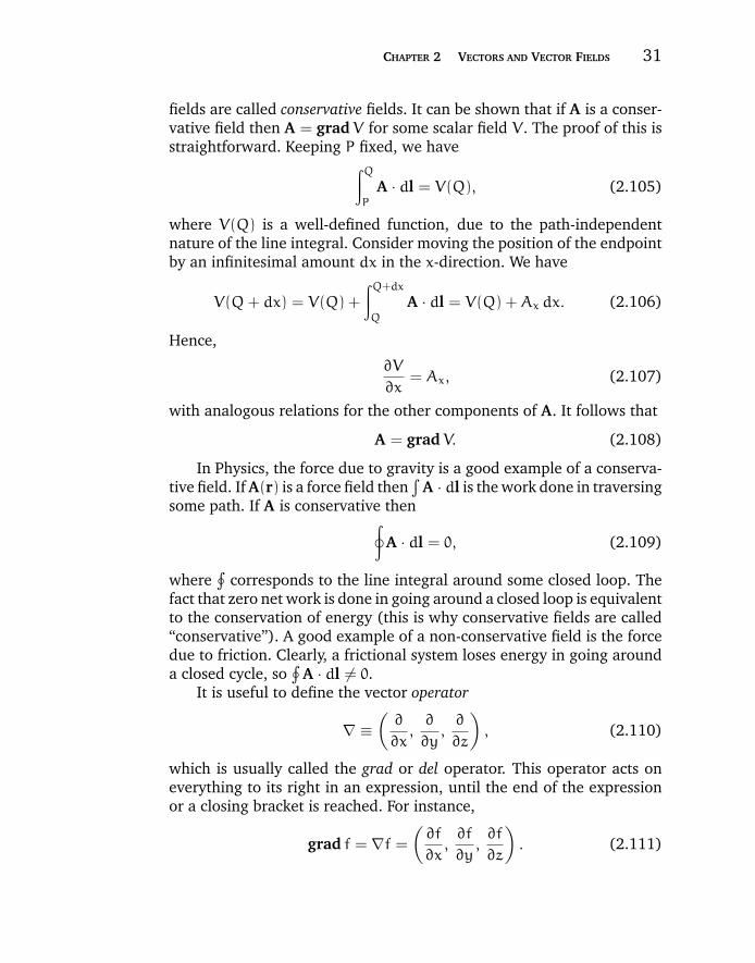
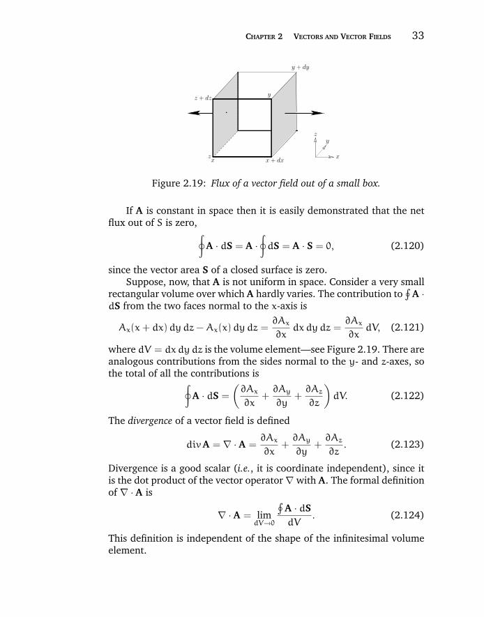
CHAPTER 2 VECTORS AND VECTOR FIELDS 33
y + dy
z
zx + dx
x
z + dzy
x
y
Figure 2.19: Flux of a vector field out of a small box.
If A is constant in space then it is easily demonstrated that the netflux out of S is zero, ∮
A · dS = A ·∮dS = A · S = 0, (2.120)
since the vector area S of a closed surface is zero.Suppose, now, that A is not uniform in space. Consider a very small
rectangular volume over which A hardly varies. The contribution to∮
A ·dS from the two faces normal to the x-axis is
Ax(x+ dx)dydz−Ax(x)dydz =∂Ax
∂xdxdydz =
∂Ax
∂xdV, (2.121)
where dV = dxdydz is the volume element—see Figure 2.19. There areanalogous contributions from the sides normal to the y- and z-axes, sothe total of all the contributions is∮
A · dS =
(∂Ax
∂x+∂Ay
∂y+∂Az
∂z
)dV. (2.122)
The divergence of a vector field is defined
divA = ∇ · A =∂Ax
∂x+∂Ay
∂y+∂Az
∂z. (2.123)
Divergence is a good scalar (i.e., it is coordinate independent), since itis the dot product of the vector operator ∇ with A. The formal definitionof ∇ · A is
∇ · A = limdV→0
∮A · dSdV
. (2.124)
This definition is independent of the shape of the infinitesimal volumeelement.
“chapter2” — 2007/11/29 — 13:42 — page 34 — #30
34 MAXWELL’S EQUATIONS AND THE PRINCIPLES OF ELECTROMAGNETISM
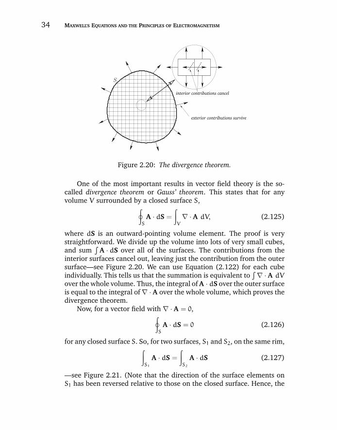
.
exterior contributions survive
S
interior contributions cancel
Figure 2.20: The divergence theorem.
One of the most important results in vector field theory is the so-called divergence theorem or Gauss’ theorem. This states that for anyvolume V surrounded by a closed surface S,∮
S
A · dS =
∫V
∇ · A dV, (2.125)
where dS is an outward-pointing volume element. The proof is verystraightforward. We divide up the volume into lots of very small cubes,and sum
∫A · dS over all of the surfaces. The contributions from the
interior surfaces cancel out, leaving just the contribution from the outersurface—see Figure 2.20. We can use Equation (2.122) for each cubeindividually. This tells us that the summation is equivalent to
∫ ∇ · A dV
over the whole volume. Thus, the integral of A · dS over the outer surfaceis equal to the integral of ∇ · A over the whole volume, which proves thedivergence theorem.
Now, for a vector field with ∇ · A = 0,∮S
A · dS = 0 (2.126)
for any closed surface S. So, for two surfaces, S1 and S2, on the same rim,∫S1
A · dS =
∫S2
A · dS (2.127)
—see Figure 2.21. (Note that the direction of the surface elements onS1 has been reversed relative to those on the closed surface. Hence, the
“chapter2” — 2007/11/29 — 13:42 — page 35 — #31
CHAPTER 2 VECTORS AND VECTOR FIELDS 35
S
rim
S2
S1
Figure 2.21: Two surfaces spanning the same rim (right), and theequivalent closed surface (left).
sign of the associated surface integral is also reversed.) Thus, if ∇ · A = 0
then the surface integral depends on the rim but not the nature of thesurface which spans it. On the other hand, if ∇ · A = 0 then the integraldepends on both the rim and the surface.
Consider an incompressible fluid whose velocity field is v. It is clearthat
∮v · dS = 0 for any closed surface, since what flows into the surface
must flow out again. Thus, according to the divergence theorem,∫ ∇ ·
v dV = 0 for any volume. The only way in which this is possible is if ∇ · vis everywhere zero. Thus, the velocity components of an incompressiblefluid satisfy the following differential relation:
∂vx
∂x+∂vy
∂y+∂vz
∂z= 0. (2.128)
Consider, now, a compressible fluid of density ρ and velocity v. Thesurface integral
∮Sρ v · dS is the net rate of mass flow out of the closed
surface S. This must be equal to the rate of decrease of mass inside thevolume V enclosed by S, which is written −(∂/∂t)(
∫VρdV). Thus,
∮S
ρ v · dS = −∂
∂t
(∫V
ρ dV
)(2.129)
for any volume. It follows from the divergence theorem that
∇·(ρ v) = −∂ρ
∂t. (2.130)
“chapter2” — 2007/11/29 — 13:42 — page 36 — #32
36 MAXWELL’S EQUATIONS AND THE PRINCIPLES OF ELECTROMAGNETISM
21
Figure 2.22: Divergent lines of force.
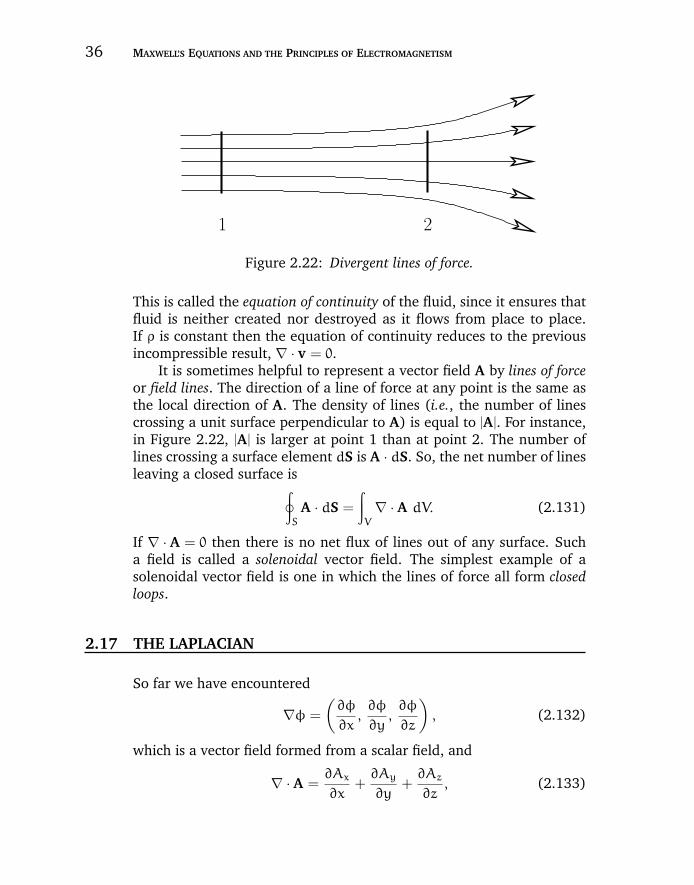
This is called the equation of continuity of the fluid, since it ensures thatfluid is neither created nor destroyed as it flows from place to place.If ρ is constant then the equation of continuity reduces to the previousincompressible result, ∇ · v = 0.
It is sometimes helpful to represent a vector field A by lines of forceor field lines. The direction of a line of force at any point is the same asthe local direction of A. The density of lines (i.e., the number of linescrossing a unit surface perpendicular to A) is equal to |A|. For instance,in Figure 2.22, |A| is larger at point 1 than at point 2. The number oflines crossing a surface element dS is A · dS. So, the net number of linesleaving a closed surface is∮
S
A · dS =
∫V
∇ · A dV. (2.131)
If ∇ · A = 0 then there is no net flux of lines out of any surface. Sucha field is called a solenoidal vector field. The simplest example of asolenoidal vector field is one in which the lines of force all form closedloops.
2.17 THE LAPLACIAN
So far we have encountered
∇φ =
(∂φ
∂x,∂φ
∂y,∂φ
∂z
), (2.132)
which is a vector field formed from a scalar field, and
∇ · A =∂Ax
∂x+∂Ay
∂y+∂Az
∂z, (2.133)
“chapter2” — 2007/11/29 — 13:42 — page 37 — #33
CHAPTER 2 VECTORS AND VECTOR FIELDS 37
which is a scalar field formed from a vector field. There are two waysin which we can combine gradient and divergence. We can either formthe vector field ∇(∇ · A) or the scalar field ∇ · (∇φ). The former is notparticularly interesting, but the scalar field ∇ · (∇φ) turns up in a greatmany problems in Physics, and is, therefore, worthy of discussion.
Let us introduce the heat-flow vector h, which is the rate of flow ofheat energy per unit area across a surface perpendicular to the directionof h. In many substances, heat flows directly down the temperaturegradient, so that we can write
h = −κ ∇T, (2.134)
where κ is the thermal conductivity. The net rate of heat flow∮S
h · dSout of some closed surface S must be equal to the rate of decrease ofheat energy in the volume V enclosed by S. Thus, we have∮
S
h · dS = −∂
∂t
(∫c T dV
), (2.135)
where c is the specific heat. It follows from the divergence theorem that
∇ · h = −c∂T
∂t. (2.136)
Taking the divergence of both sides of Equation (2.134), and makinguse of Equation (2.136), we obtain
∇ · (κ∇T) = c∂T
∂t. (2.137)
If κ is constant then the above equation can be written
∇ · (∇T) =c
κ
∂T
∂t. (2.138)
The scalar field ∇ · (∇T) takes the form
∇ · (∇T) =∂
∂x
(∂T
∂x
)+∂
∂y
(∂T
∂y
)+∂
∂z
(∂T
∂z
)
=∂2T
∂x2+∂2T
∂y2+∂2T
∂z2≡ ∇2T. (2.139)
Here, the scalar differential operator
∇2 ≡ ∂2
∂x2+∂2
∂y2+∂2
∂z2(2.140)
“chapter2” — 2007/11/29 — 13:42 — page 38 — #34
38 MAXWELL’S EQUATIONS AND THE PRINCIPLES OF ELECTROMAGNETISM
is called the Laplacian. The Laplacian is a good scalar operator (i.e., itis coordinate independent) because it is formed from a combination ofdivergence (another good scalar operator) and gradient (a good vectoroperator).
What is the physical significance of the Laplacian? In one dimension,∇2T reduces to ∂2T/∂x2. Now, ∂2T/∂x2 is positive if T(x) is concave (fromabove) and negative if it is convex. So, if T is less than the average of Tin its surroundings then ∇2T is positive, and vice versa.
In two dimensions,
∇2T =∂2T
∂x2+∂2T
∂y2. (2.141)
Consider a local minimum of the temperature. At the minimum, theslope of T increases in all directions, so ∇2T is positive. Likewise, ∇2T isnegative at a local maximum. Consider, now, a steep-sided valley in T .Suppose that the bottom of the valley runs parallel to the x-axis. Atthe bottom of the valley ∂2T/∂y2 is large and positive, whereas ∂2T/∂x2
is small and may even be negative. Thus, ∇2T is positive, and this isassociated with T being less than the average local value.
Let us now return to the heat conduction problem:
∇2T =c
κ
∂T
∂t. (2.142)
It is clear that if ∇2T is positive then T is locally less than the averagevalue, so ∂T/∂t > 0: i.e., the region heats up. Likewise, if ∇2T is negativethen T is locally greater than the average value, and heat flows out ofthe region: i.e., ∂T/∂t < 0. Thus, the above heat conduction equationmakes physical sense.
2.18 CURL
Consider a vector field A(r), and a loop which lies in one plane. Theintegral of A around this loop is written
∮A · dl, wheredl is a line element
of the loop. If A is a conservative field then A = ∇φ and∮
A · dl = 0 forall loops. In general, for a non-conservative field,
∮A · dl = 0.
For a small loop we expect∮
A · dl to be proportional to the area ofthe loop. Moreover, for a fixed-area loop we expect
∮A · dl to depend
on the orientation of the loop. One particular orientation will give themaximum value:
∮A · dl = Imax. If the loop subtends an angle θ with
“chapter2” — 2007/11/29 — 13:42 — page 39 — #35
CHAPTER 2 VECTORS AND VECTOR FIELDS 39
z
z + dz
1
4
3
zy 2 y + dy
y
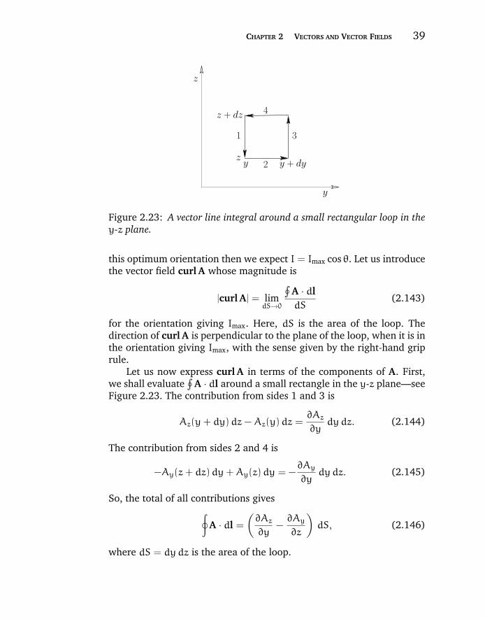
Figure 2.23: A vector line integral around a small rectangular loop in they-z plane.
this optimum orientation then we expect I = Imax cos θ. Let us introducethe vector field curl A whose magnitude is
|curl A| = limdS→0
∮A · dldS
(2.143)
for the orientation giving Imax. Here, dS is the area of the loop. Thedirection of curl A is perpendicular to the plane of the loop, when it is inthe orientation giving Imax, with the sense given by the right-hand griprule.
Let us now express curl A in terms of the components of A. First,we shall evaluate
∮A · dl around a small rectangle in the y-z plane—see
Figure 2.23. The contribution from sides 1 and 3 is
Az(y+ dy)dz−Az(y)dz =∂Az
∂ydydz. (2.144)
The contribution from sides 2 and 4 is
−Ay(z+ dz)dy+Ay(z)dy = −∂Ay
∂ydydz. (2.145)
So, the total of all contributions gives∮A · dl =
(∂Az
∂y−∂Ay
∂z
)dS, (2.146)
where dS = dydz is the area of the loop.
“chapter2” — 2007/11/29 — 13:42 — page 40 — #36
40 MAXWELL’S EQUATIONS AND THE PRINCIPLES OF ELECTROMAGNETISM
Consider a non-rectangular (but still small) loop in the y-z plane.We can divide it into rectangular elements, and form
∮A · dl over all the
resultant loops. The interior contributions cancel, so we are just left withthe contribution from the outer loop. Also, the area of the outer loop isthe sum of all the areas of the inner loops. We conclude that
∮A · dl =
(∂Az
∂y−∂Ay
∂z
)dSx (2.147)
is valid for a small loop dS = (dSx, 0, 0) of any shape in the y-z plane.Likewise, we can show that if the loop is in the x-z plane then dS =(0, dSy, 0) and
∮A · dl =
(∂Ax
∂z−∂Az
∂x
)dSy. (2.148)
Finally, if the loop is in the x-y plane then dS = (0, 0, dSz) and
∮A · dl =
(∂Ay
∂x−∂Ax
∂y
)dSz. (2.149)
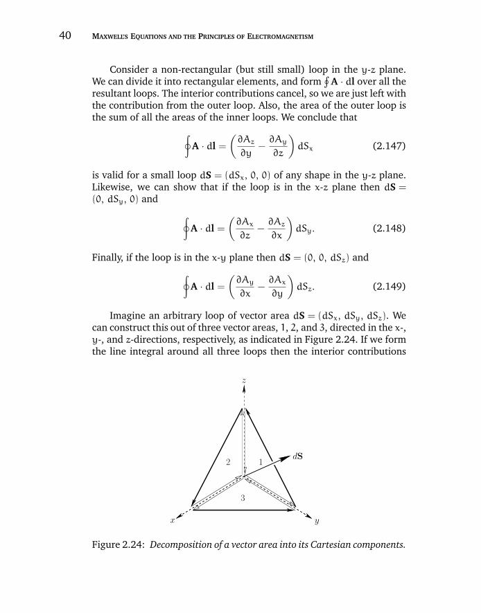
Imagine an arbitrary loop of vector area dS = (dSx, dSy, dSz). Wecan construct this out of three vector areas, 1, 2, and 3, directed in the x-,y-, and z-directions, respectively, as indicated in Figure 2.24. If we formthe line integral around all three loops then the interior contributions
dS
yx
3
2 1
z
Figure 2.24: Decomposition of a vector area into its Cartesian components.
“chapter2” — 2007/11/29 — 13:42 — page 41 — #37
CHAPTER 2 VECTORS AND VECTOR FIELDS 41
cancel, and we are left with the line integral around the original loop.Thus, ∮
A · dl =
∮A · dl1 +
∮A · dl2 +
∮A · dl3, (2.150)
giving ∮A · dl = curl A · dS = |curl A| |dS| cos θ, (2.151)
where
curl A =
(∂Az
∂y−∂Ay
∂z,∂Ax
∂z−∂Az
∂x,∂Ay
∂x−∂Ax
∂y
), (2.152)
and θ is the angle subtended between the directions of curl A and dS.Note that
curl A = ∇ × A =
∣∣∣∣∣∣∣ex ey ez∂/∂x ∂/∂y ∂/∂z
Ax Ay Az
∣∣∣∣∣∣∣ . (2.153)
This demonstrates that ∇ × A is a good vector field, since it is the crossproduct of the ∇ operator (a good vector operator) and the vector field A.
Consider a solid body rotating about the z-axis. The angular velocityis given by ω = (0, 0, ω), so the rotation velocity at position r is
v = ω × r (2.154)
[see Equation (2.44)]. Let us evaluate ∇ × v on the axis of rotation.The x-component is proportional to the integral
∮v · dl around a loop
in the y-z plane. This is plainly zero. Likewise, the y-component is alsozero. The z-component is
∮v · dl/dS around some loop in the x-y plane.
Consider a circular loop. We have∮
v · dl = 2π rω rwithdS = π r2. Here,r is the perpendicular distance from the rotation axis. It follows that(∇ × v)z = 2ω, which is independent of r. So, on the axis, ∇ × v =(0 , 0 , 2ω). Off the axis, at position r0, we can write
v = ω × (r − r0) + ω × r0. (2.155)
The first part has the same curl as the velocity field on the axis, and thesecond part has zero curl, since it is constant. Thus, ∇ × v = (0, 0, 2ω)everywhere in the body. This allows us to form a physical picture of
“chapter2” — 2007/11/29 — 13:42 — page 42 — #38
42 MAXWELL’S EQUATIONS AND THE PRINCIPLES OF ELECTROMAGNETISM
∇ × A. If we imagine A(r) as the velocity field of some fluid, then ∇ × Aat any given point is equal to twice the local angular rotation velocity:i.e., 2 ω. Hence, a vector field with ∇ × A = 0 everywhere is said to beirrotational.
Another important result of vector field theory is the curl theorem orStokes’ theorem: ∮
C
A · dl =
∫S
∇ × A · dS, (2.156)
for some (non-planar) surface S bounded by a rim C. This theorem caneasily be proved by splitting the loop up into many small rectangularloops, and forming the integral around all of the resultant loops. All of thecontributions from the interior loops cancel, leaving just the contributionfrom the outer rim. Making use of Equation (2.151) for each of the smallloops, we can see that the contribution from all of the loops is also equalto the integral of ∇ × A · dS across the whole surface. This proves thetheorem.
One immediate consequence of Stokes’ theorem is that ∇ × A is“incompressible.” Consider any two surfaces, S1 and S2, which share thesame rim—see Figure 2.21. It is clear from Stokes’ theorem that
∫ ∇ ×A · dS is the same for both surfaces. Thus, it follows that
∮ ∇ × A · dS = 0
for any closed surface. However, we have from the divergence theoremthat
∮ ∇ × A · dS =∫ ∇ · (∇ × A)dV = 0 for any volume. Hence,
∇ · (∇ × A) ≡ 0. (2.157)
So, ∇ × A is a solenoidal field.We have seen that for a conservative field
∮A · dl = 0 for any loop.
This is entirely equivalent to A = ∇φ. However, the magnitude of ∇ × Ais lim dS→0
∮A · dl/dS for some particular loop. It is clear then that ∇ ×
A = 0 for a conservative field. In other words,
∇ × (∇φ) ≡ 0. (2.158)
Thus, a conservative field is also an irrotational one.Finally, it can be shown that
∇ × (∇ × A) = ∇(∇ · A) − ∇2A, (2.159)
where
∇2A = (∇2Ax, ∇2Ay, ∇2Az). (2.160)
It should be emphasized, however, that the above result is only valid inCartesian coordinates.

“chapter2” — 2007/11/29 — 13:42 — page 43 — #39
CHAPTER 2 VECTORS AND VECTOR FIELDS 43
z
θ
y
x
eθ
r
er
Figure 2.25: Cylindrical polar coordinates.
2.19 POLAR COORDINATES
In the cylindrical polar coordinate system the Cartesian coordinates xand y are replaced by r =
√x2 + y2 and θ = tan−1(y/x). Here, r is
the perpendicular distance from the z-axis, and θ the angle subtendedbetween the perpendicular radius vector and the x-axis—see Figure 2.25.A general vector A is thus written
A = Ar er +Aθ eθ +Az ez, (2.161)
where er = ∇r/|∇r| and eθ = ∇θ/|∇θ|—see Figure 2.25. Note that theunit vectors er, eθ, and ez are mutually orthogonal. Hence, Ar = A · er,etc. The volume element in this coordinate system is d3r = r dr dθdz.Moreover, gradient, divergence, and curl take the form
∇V =∂V
∂rer +
1
r
∂V
∂θeθ +
∂V
∂zez, (2.162)
∇ · A =1
r
∂
∂r(rAr) +
1
r
∂Aθ
∂θ+∂Az
∂z, (2.163)

“chapter2” — 2007/11/29 — 13:42 — page 44 — #40
44 MAXWELL’S EQUATIONS AND THE PRINCIPLES OF ELECTROMAGNETISM
∇ × A =
(1
r
∂Az
∂θ−∂Aθ
∂z
)er +
(∂Ar
∂z−∂Az
∂r
)eθ
+
(1
r
∂
∂r(rAθ) −
1
r
∂Ar
∂θ
)ez, (2.164)
respectively. Here, V(r) is a general vector field, and A(r) a general scalarfield. Finally, the Laplacian is written
∇2V =1
r
∂
∂r
(r∂V
∂r
)+1
r2∂2V
∂θ2+∂2V
∂z2. (2.165)
In the spherical polar coordinate system the Cartesian coordinatesx, y, and z are replaced by r =
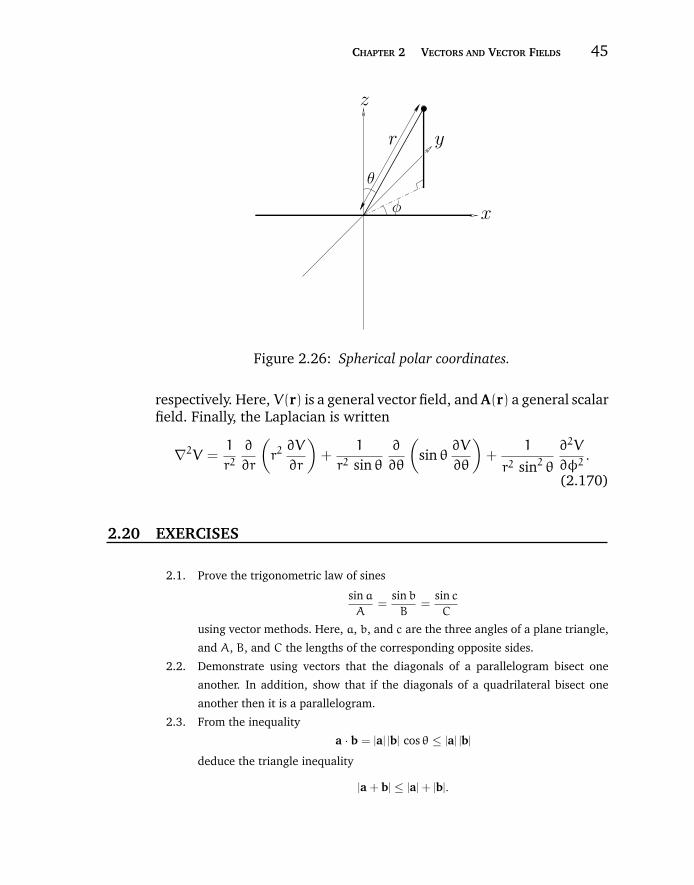
√x2 + y2 + z2, θ = cos−1(z/r), and φ =
tan−1(y/x). Here, r is the distance from the origin, θ the angle subtendedbetween the radius vector and the z-axis, and φ the angle subtendedbetween the projection of the radius vector onto the x-y plane and the x-axis—see Figure 2.26. Note that r and θ in the spherical polar system arenot the same as their counterparts in the cylindrical system. A generalvector A is written
A = Ar er +Aθ eθ +Aφ eφ, (2.166)
where er = ∇r/|∇r|, eθ = ∇θ/|∇θ|, and eφ = ∇φ/|∇φ|. The unit vec-tors er, eθ, and eφ are mutually orthogonal. Hence, Ar = A · er, etc.The volume element in this coordinate system is d3r = r2 sin θdr dθdφ.Moreover, gradient, divergence, and curl take the form
∇V =∂V
∂rer +
1
r
∂V
∂θeθ +
1
r sin θ∂V
∂φeφ, (2.167)
∇ · A =1
r2∂
∂r(r2 Ar) +
1
r sin θ∂
∂θ(sin θAθ)
+1
r sin θ∂Aφ
∂φ, (2.168)
∇ × A =
(1
r sin θ∂
∂θ(sin θAφ) −
1
r sin θ∂Aθ
∂φ
)er
+
(1
r sin θ∂Ar
∂φ−1
r
∂
∂r(rAφ)
)eθ
+
(1
r
∂
∂r(rAθ) −
1
r
∂Ar
∂θ
)eφ, (2.169)
“chapter2” — 2007/11/29 — 13:42 — page 45 — #41
CHAPTER 2 VECTORS AND VECTOR FIELDS 45
r y
xφ
θ
z
Figure 2.26: Spherical polar coordinates.
respectively. Here, V(r) is a general vector field, and A(r) a general scalarfield. Finally, the Laplacian is written
∇2V =1
r2∂
∂r
(r2∂V
∂r
)+
1
r2 sin θ∂
∂θ
(sin θ
∂V
∂θ
)+
1
r2 sin2 θ∂2V
∂φ2.
(2.170)
2.20 EXERCISES
2.1. Prove the trigonometric law of sines
sin aA
=sin bB
=sin cC
using vector methods. Here, a, b, and c are the three angles of a plane triangle,
and A, B, and C the lengths of the corresponding opposite sides.
2.2. Demonstrate using vectors that the diagonals of a parallelogram bisect one
another. In addition, show that if the diagonals of a quadrilateral bisect one
another then it is a parallelogram.
2.3. From the inequality
a · b = |a| |b| cos θ ≤ |a| |b|
deduce the triangle inequality
|a + b| ≤ |a| + |b|.
“chapter2” — 2007/11/29 — 13:42 — page 46 — #42
46 MAXWELL’S EQUATIONS AND THE PRINCIPLES OF ELECTROMAGNETISM
2.4. Identify the following surfaces:
(a) |r| = a,
(b) r · n = b,
(c) r · n = c |r|,
(d) |r − (r · n) n| = d.
Here, r is the position vector, a, b, c, and d are positive constants, and n is a
fixed unit vector.
2.5. Let a, b, and c be coplanar vectors related via
α a + βb + γ c = 0,
where α, β, and γ are not all zero. Show that the condition for the points with
position vectors u a, vb, and w c to be colinear is
α
u+β
v+γ
w= 0.
2.6. If p, q, and r are any vectors, demonstrate that a = q + λ r, b = r + µp, and
c = p + νq are coplanar provided that λµν = −1, where λ, µ, and ν are scalars.
Show that this condition is satisfied when a is perpendicular to p, b to q, and c
to r.
2.7. The vectors a, b, and c are not coplanar, and form a non-orthogonal vector base.
The vectors A, B, and C, defined by
A =b × c
a · b × c,
plus cyclic permutations, are said to be reciprocal vectors. Show that
a = (B × C)/(A · B × C),
plus cyclic permutations.
2.8. In the notation of the previous question, demonstrate that the plane passing
through points a/α, b/β, and c/γ is normal to the direction of the vector
h = αA + βB + γC.
In addition, show that the perpendicular distance of the plane from the origin
is |h|−1.
2.9. A ray of light moving in the direction k impinges on a surface at a point where
its normal is n. If k ′ is the direction of the refracted ray, then Snell’s law (in
vector form) gives
µ k × n = µ′ k ′ × n,
where µ and µ ′ are the refractive indices of the media on either side of the
surface. Note that k, k ′, and n are unit vectors: i.e., they all have unit length.
“chapter2” — 2007/11/29 — 13:42 — page 47 — #43
CHAPTER 2 VECTORS AND VECTOR FIELDS 47
Show that k ′ is in the plane of k and n, and that
k ′ =µ
µ ′ [k − (k · n) n + θn] ,
where
θ2 = (k · n)2 +
(µ ′
µ
)2
− 1.
Which sign of the square-root must be taken? Under what circumstances is θ
imaginary, and what does this imply physically?
2.10. Consider the following vector field:
A(r) = (8 x3 + 3 x2 y2, 2 x3 y + 6 y, 6).
Is this field conservative? Is it solenoidal? Is it irrotational? Justify your answers.
Calculate∮C
A · dr, where the curve C is a unit circle in the x-y plane, centered
on the origin, and the direction of integration is clockwise looking down the
z-axis.
2.11. Consider the following vector field:
A(r) = (3 x y2 z2 − y2, −y3 z2 + x2 y, 3 x2 − x2 z).
Is this field conservative? Is it solenoidal? Is it irrotational? Justify your answers.
Calculate the flux of A out of a unit sphere centered on the origin.
2.12. Find the gradients of the following scalar functions of the position vector r =
(x, y, z):
(a) k · r,
(b) |r|n,
(c) |r − k|−n,
(d) cos(k · r).
Here, k is a fixed vector.
2.13. Find the divergences and curls of the following vector fields:
(a) k × r,
(b) |r|n r,
(c) |r − k|n (r − k),
(d) a cos(k · r).
Here, k and a are fixed vectors.
2.14. Calculate ∇2φ when φ = f(|r|). Find f if ∇2φ = 0.
2.15. Find the Cartesian components of the basis vectors er, eθ, and ez of the cylindrical
polar coordinate system. Verify that the vectors are mutually orthogonal. Do the
same for the basis vectors er, eθ, and eφ of the spherical polar coordinate system.

“chapter2” — 2007/11/29 — 13:42 — page 48 — #44
“chapter3” — 2007/12/14 — 12:02 — page 49 — #1
C h a p t e r 3 TIME-INDEPENDENTMAXWELL EQUATIONS
3.1 INTRODUCTION
In this chapter, we shall recast the familiar force laws of electrostaticsand magnetostatics as vector field equations.
3.2 COULOMB’S LAW
Between 1785 and 1787, the French physicist Charles Augustine deCoulomb performed a series of experiments involving electric charges,and eventually established what is nowadays known as Coulomb’s law.According to this law, the force acting between two static electric chargesis central, inverse-square, and proportional to the product of the charges.Two like charges repel one another, whereas two unlike charges attract.Suppose that two charges, q1 and q2, are located at position vectors r1and r2, respectively. The electrical force acting on the second charge iswritten
f2 =q1 q2
4πε0
r2 − r1|r2 − r1|3
(3.1)
in vector notation—see Figure 3.1. An equal and opposite force acts onthe first charge, in accordance with Newton’s third law of motion. The SIunit of electric charge is the coulomb (C). The magnitude of the chargeon an electron is 1.6022× 10⁻¹⁹ C. Finally, the universal constant ε0 iscalled the permittivity of free space, and takes the value
ε0 = 8.8542× 10⁻¹² C 2 N−1m−2. (3.2)
Suppose that two masses, m1 and m2, are located at position vec-tors r1 and r2, respectively. According to Newton’s law of gravity, thegravitational force acting on the second mass is written
f2 = −Gm1m2r2 − r1
|r2 − r1|3(3.3)
49
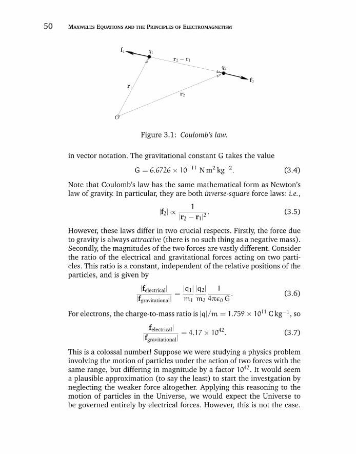
“chapter3” — 2007/12/14 — 12:02 — page 50 — #2
50 MAXWELL’S EQUATIONS AND THE PRINCIPLES OF ELECTROMAGNETISM
r1
r2 − r1
r2
q1f1
f2
q2
O
Figure 3.1: Coulomb’s law.
in vector notation. The gravitational constant G takes the value
G = 6.6726× 10⁻¹¹ N m2 kg−2. (3.4)
Note that Coulomb’s law has the same mathematical form as Newton’slaw of gravity. In particular, they are both inverse-square force laws: i.e.,
|f2| ∝ 1
|r2 − r1|2. (3.5)
However, these laws differ in two crucial respects. Firstly, the force dueto gravity is always attractive (there is no such thing as a negative mass).Secondly, the magnitudes of the two forces are vastly different. Considerthe ratio of the electrical and gravitational forces acting on two parti-cles. This ratio is a constant, independent of the relative positions of theparticles, and is given by
|felectrical|
|fgravitational|=
|q1|
m1
|q2|
m2
1
4πε0 G. (3.6)
For electrons, the charge-to-mass ratio is |q|/m = 1.759× 10¹¹ C kg−1, so
|felectrical|
|fgravitational|= 4.17× 1042. (3.7)
This is a colossal number! Suppose we were studying a physics probleminvolving the motion of particles under the action of two forces with thesame range, but differing in magnitude by a factor 1042. It would seema plausible approximation (to say the least) to start the investgation byneglecting the weaker force altogether. Applying this reasoning to themotion of particles in the Universe, we would expect the Universe tobe governed entirely by electrical forces. However, this is not the case.
“chapter3” — 2007/12/14 — 12:02 — page 51 — #3
CHAPTER 3 TIME-INDEPENDENT MAXWELL EQUATIONS 51
The force which holds us to the surface of the Earth, and prevents usfrom floating off into space, is gravity. The force which causes the Earthto orbit the Sun is also gravity. In fact, on astronomical length-scalesgravity is the dominant force, and electrical forces are largely irrelevant.The key to understanding this paradox is that there are both positive andnegative electric charges, whereas there are only positive gravitational“charges.” This means that gravitational forces are always cumulative,whereas electrical forces can cancel one another out. Suppose, for thesake of argument, that the Universe starts out with randomly distributedelectric charges. Initially, we expect electrical forces to completely dom-inate gravity. These forces try to make every positive charge get as faraway as possible from the other positive charges in the Universe, and asclose as possible to the other negative charges. After a while, we expectthe positive and negative charges to form close pairs. Just how close isdetermined by Quantum Mechanics, but, in general, it is fairly close:i.e., about 10−10 m. The electrical forces due to the charges in each paireffectively cancel one another out on length-scales much larger than themutual spacing of the pair. However, it is only possible for gravity to bethe dominant long-range force in the Universe if the number of positivecharges is almost equal to the number of negative charges. In this situ-ation, every positive charge can find a negative charge to team up with,and there are virtually no charges left over. In order for the cancellationof long-range electrical forces to be effective, the relative difference inthe number of positive and negative charges in the Universe must beincredibly small. In fact, positive and negative charges have to cancelone another to such accuracy that most physicists believe that the netelectrical charge of the Universe is exactly zero. But, it is not sufficientfor the Universe to start out with zero charge. Suppose there were someelementary particle process which did not conserve electric charge. Evenif this were to go on at a very low rate, it would not take long before thefine balance between positive and negative charges in the Universe waswrecked. So, it is important that electric charge is a conserved quantity(i.e., the net charge of the Universe can neither increase or decrease). Asfar as we know, this is the case. To date, no elementary particle reactionshave been discovered which create or destroy net electric charge.
In summary, there are two long-range forces in the Universe, elec-tricity and gravity. The former is enormously stronger than the latter, butis usually “hidden” away inside neutral atoms. The fine balance of forcesdue to negative and positive electric charges starts to break down onatomic scales. In fact, interatomic and intermolecular forces are all elec-trical in nature. So, electrical forces are basically what prevent us from
“chapter3” — 2007/12/14 — 12:02 — page 52 — #4
52 MAXWELL’S EQUATIONS AND THE PRINCIPLES OF ELECTROMAGNETISM
falling though the floor. But, this is electromagnetism on the microscopicor atomic scale—what is usually termed Quantum Electromagnetism. Thisbook is about Classical Electromagnetism. That is, electromagnetism onlength-scales much larger than the atomic scale. Classical Electromag-netism generally describes phenomena in which some sort of “violence”is done to matter, so that the close pairing of negative and positivecharges is disrupted. This allows electrical forces to manifest themselveson macroscopic length-scales. Of course, very little disruption is neces-sary before gigantic forces are generated. Hence, it is no coincidencethat the vast majority of useful machines which humankind has devisedduring the last century or so are electrical in nature.
Coulomb’s law and Newton’s law are both examples of what are usu-ally referred to as action-at-a-distance laws. According to Equations (3.1)and (3.3), if the first charge or mass is moved then the force acting onthe second charge or mass responds immediately. In particular, equal andopposite forces act on the two charges or masses at all times. However,this cannot be correct according to Einstein’s Special Theory of Relativ-ity, which implies that the maximum speed with which information canpropagate through the Universe is the speed of light in vacuum. So, if thefirst charge or mass is moved then there must always be a time delay (i.e.,at least the time needed for a light signal to propagate between the twocharges or masses) before the second charge or mass responds. Considera rather extreme example. Suppose the first charge or mass is suddenlyannihilated. The second charge or mass only finds out about this sometime later. During this time interval, the second charge or mass experi-ences an electrical or gravitational force which is as if the first chargeor mass were still there. So, during this period, there is an action butno reaction, which violates Newton’s third law of motion. It is clear thataction at a distance is not compatible with Relativity, and, consequently,that Newton’s third law of motion is not strictly true. Of course, Newton’sthird law is intimately tied up with the conservation of linear momen-tum in the Universe. This is a concept which most physicists are loath toabandon. It turns out that we can “rescue” momentum conservation byabandoning action-at-a-distance theories, and instead adopting so-calledfield theories in which there is a medium, called a field, which transmitsthe force from one particle to another. Of course, in electromagnetismthere are two fields—the electric field, and the magnetic field. Electro-magnetic forces are transmitted via these fields at the speed of light,which implies that the laws of Relativity are never violated. Moreover,the fields can soak up energy and momentum. This means that evenwhen the actions and reactions acting on charged particles are not quiteequal and opposite, momentum is still conserved. We can bypass some
“chapter3” — 2007/12/14 — 12:02 — page 53 — #5
CHAPTER 3 TIME-INDEPENDENT MAXWELL EQUATIONS 53
of the problematic aspects of action at a distance by only consideringsteady-state situations. For the moment, this is how we shall proceed.
Consider N charges, q1 though qN, which are located at positionvectors r1 through rN, respectively. Electrical forces obey what is knownas the principle of superposition: i.e., the electrical force acting on a testchargeq at position vector r is simply the vector sum of all of the Coulomblaw forces exerted on it by each of the N charges taken in isolation. Inother words, the electrical force exerted by the ith charge (say) on thetest charge is the same as if all of the other charges were not there. Thus,the force acting on the test charge is given by
f(r) = q
N∑i=1
qi
4πε0
r − ri|r − ri|3
. (3.8)
It is helpful to define a vector field E(r), called the electric field, which isthe force exerted on a unit test charge located at position vector r. So,the force on a test charge is written
f = qE, (3.9)
and the electric field is given by
E(r) =
N∑i=1
qi
4πε0
r − ri|r − ri|3
. (3.10)
At this point, we have no reason to believe that the electric field has anyreal physical existence. It is just a useful device for calculating the forcewhich acts on test charges placed at various locations.
The electric field from a single charge q located at the origin is purelyradial, points outward if the charge is positive, inward if it is negative,and has magnitude
Er(r) =q
4πε0 r2, (3.11)
where r = |r|. We can represent an electric field by field-lines. The direc-tion of the lines indicates the direction of the local electric field, and thedensity of the lines perpendicular to this direction is proportional to themagnitude of the local electric field. It follows from Equation (3.11) thatthe number of field-lines crossing the surface of a sphere centered on apoint charge (which is equal to Er times the area, 4π r2, of the surface) isindependent of the radius of the sphere. Thus, the field of a point positivecharge is represented by a group of equally spaced, unbroken, straight
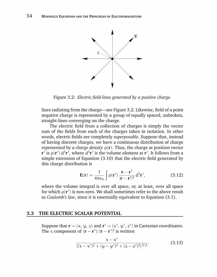
“chapter3” — 2007/12/14 — 12:02 — page 54 — #6
54 MAXWELL’S EQUATIONS AND THE PRINCIPLES OF ELECTROMAGNETISM
E
q
Figure 3.2: Electric field-lines generated by a positive charge.
lines radiating from the charge—see Figure 3.2. Likewise, field of a pointnegative charge is represented by a group of equally spaced, unbroken,straight-lines converging on the charge.
The electric field from a collection of charges is simply the vectorsum of the fields from each of the charges taken in isolation. In otherwords, electric fields are completely superposable. Suppose that, insteadof having discrete charges, we have a continuous distribution of chargerepresented by a charge density ρ(r). Thus, the charge at position vectorr ′ is ρ(r ′)d3r ′, where d3r ′ is the volume element at r ′. It follows from asimple extension of Equation (3.10) that the electric field generated bythis charge distribution is
E(r) =1
4πε0
∫ρ(r ′)
r − r ′
|r − r ′|3d3r ′, (3.12)
where the volume integral is over all space, or, at least, over all spacefor which ρ(r ′) is non-zero. We shall sometimes refer to the above resultas Coulomb’s law, since it is essentially equivalent to Equation (3.1).
3.3 THE ELECTRIC SCALAR POTENTIAL
Suppose that r = (x, y, z) and r ′ = (x ′, y ′, z ′) in Cartesian coordinates.The x component of (r − r ′)/|r − r ′|3 is written
x− x ′
[(x− x ′)2 + (y− y ′)2 + (z− z ′)2] 3/2. (3.13)
“chapter3” — 2007/12/14 — 12:02 — page 55 — #7
CHAPTER 3 TIME-INDEPENDENT MAXWELL EQUATIONS 55
However, it is easily demonstrated that
x− x ′
[(x− x ′)2 + (y− y ′)2 + (z− z ′)2] 3/2(3.14)
= −∂
∂x
(1
[(x− x ′)2 + (y− y ′)2 + (z− z ′)2] 1/2
).
Since there is nothing special about the x-axis, we can write
r − r ′
|r − r ′|3= −∇
(1
|r − r ′|
), (3.15)
where ∇ ≡ (∂/∂x, ∂/∂y, ∂/∂z) is a differential operator which involvesthe components of r but not those of r ′. It follows from Equation (3.12)that
E = −∇φ, (3.16)
where
φ(r) =1
4πε0
∫ρ(r ′)
|r − r ′|d3r ′. (3.17)
Thus, the electric field generated by a collection of fixed charges canbe written as the gradient of a scalar field—known as the electric scalarpotential—and this field can be expressed as a simple volume integralinvolving the charge distribution.
The scalar potential generated by a charge q located at the origin is
φ(r) =q
4πε0 r. (3.18)
According to Equation (3.10), the scalar potential generated by a set ofN discrete charges qi, located at ri, is
φ(r) =
N∑i=1
φi(r), (3.19)
where
φi(r) =qi
4πε0 |r − ri|. (3.20)
Thus, the scalar potential is just the sum of the potentials generated byeach of the charges taken in isolation.
“chapter3” — 2007/12/14 — 12:02 — page 56 — #8
56 MAXWELL’S EQUATIONS AND THE PRINCIPLES OF ELECTROMAGNETISM
Suppose that a particle of charge q is taken along some path frompoint P to point Q. The net work done on the particle by electricalforces is
W =
∫QP
f · dl, (3.21)
where f is the electrical force, and dl is a line element along the path.Making use of Equations (3.9) and (3.16), we obtain
W = q
∫QP
E · dl = −q
∫QP
∇φ · dl = −q [φ(Q) − φ(P) ] . (3.22)
Thus, the work done on the particle is simply minus its charge times thedifference in electric potential between the end point and the beginningpoint. This quantity is clearly independent of the path taken between PandQ. So, an electric field generated by stationary charges is an exampleof a conservative field. In fact, this result follows immediately from vectorfield theory once we are told, in Equation (3.16), that the electric fieldis the gradient of a scalar potential. The work done on the particle whenit is taken around a closed loop is zero, so∮
C
E · dl = 0 (3.23)
for any closed loop C. This implies from Stokes’ theorem that
∇ × E = 0 (3.24)
for any electric field generated by stationary charges. Equation (3.24)also follows directly from Equation (3.16), since ∇ × ∇φ ≡ 0 for anyscalar potential φ.
The SI unit of electric potential is the volt, which is equivalent toa joule per coulomb. Thus, according to Equation (3.22), the electri-cal work done on a particle when it is taken between two points isthe product of minus its charge and the voltage difference between thepoints.
We are familiar with the idea that a particle moving in a gravitationalfield possesses potential energy as well as kinetic energy. If the particlemoves from point P to a lower point Q then the gravitational field doeswork on the particle causing its kinetic energy to increase. The increasein kinetic energy of the particle is balanced by an equal decrease in itspotential energy, so that the overall energy of the particle is a conserved
“chapter3” — 2007/12/14 — 12:02 — page 57 — #9
CHAPTER 3 TIME-INDEPENDENT MAXWELL EQUATIONS 57
quantity. Therefore, the work done on the particle as it moves from P toQ is minus the difference in its gravitational potential energy betweenpointsQ and P. Of course, it only makes sense to talk about gravitationalpotential energy because the gravitational field is conservative. Thus, thework done in taking a particle between two points is path independent,and, therefore, well-defined. This means that the difference in poten-tial energy of the particle between the beginning and end points is alsowell-defined. We have already seen that an electric field generated bystationary charges is a conservative field. In follows that we can define anelectrical potential energy of a particle moving in such a field. By anal-ogy with gravitational fields, the work done in taking a particle frompoint P to point Q is equal to minus the difference in potential energyof the particle between points Q and P. It follows from Equation (3.22)that the potential energy of the particle at a general point Q, relativeto some reference point P (where the potential energy is set to zero), isgiven by
W(Q) = qφ(Q). (3.25)
Free particles try to move down gradients of potential energy, in orderto attain a minimum potential energy state. Thus, free particles in theEarth’s gravitational field tend to fall downward. Likewise, positivecharges moving in an electric field tend to migrate toward regions withthe most negative voltage, and vice versa for negative charges.
The scalar electric potential is undefined to an additive constant. So,the transformation
φ(r) → φ(r) + c (3.26)
leaves the electric field unchanged according to Equation (3.16). Thepotential can be fixed unambiguously by specifying its value at a singlepoint. The usual convention is to say that the potential is zero at infinity.This convention is implicit in Equation (3.17), where it can be seen thatφ → 0 as |r| → ∞, provided that the total charge
∫ρ(r ′)d3r ′ is finite.
3.4 GAUSS’ LAW
Consider a single charge q located at the origin. The electric field gen-erated by such a charge is given by Equation (3.11). Suppose that wesurround the charge by a concentric spherical surface S of radius r—see
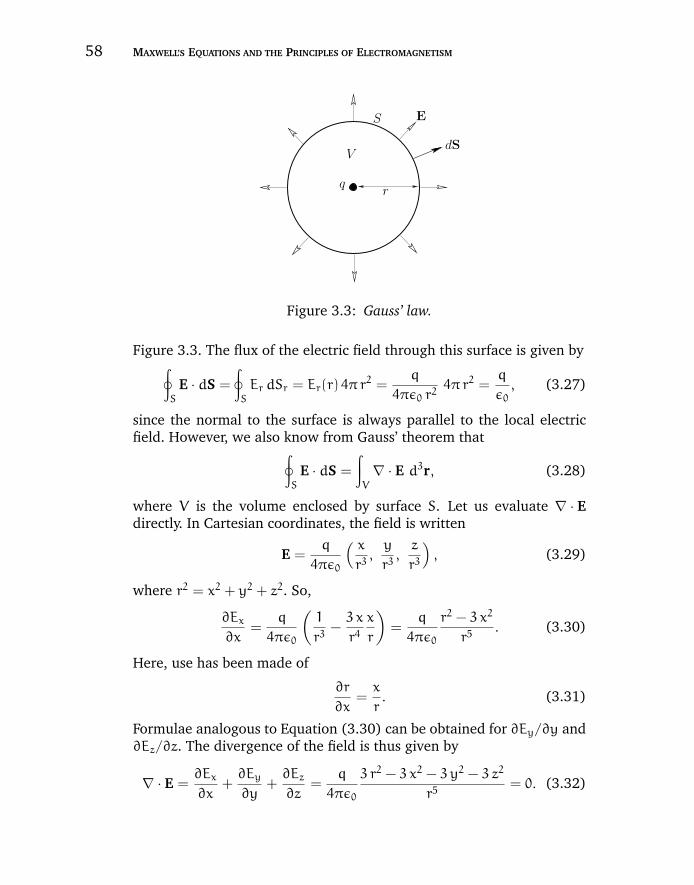
“chapter3” — 2007/12/14 — 12:02 — page 58 — #10
58 MAXWELL’S EQUATIONS AND THE PRINCIPLES OF ELECTROMAGNETISM
dS
ES
qr
V
Figure 3.3: Gauss’ law.
Figure 3.3. The flux of the electric field through this surface is given by∮S
E · dS =
∮S
Er dSr = Er(r) 4π r2 =
q
4πε0 r24π r2 =
q
ε0, (3.27)
since the normal to the surface is always parallel to the local electricfield. However, we also know from Gauss’ theorem that∮
S
E · dS =
∫V
∇ · E d3r, (3.28)
where V is the volume enclosed by surface S. Let us evaluate ∇ · Edirectly. In Cartesian coordinates, the field is written
E =q
4πε0
( xr3,y
r3,z
r3
), (3.29)
where r2 = x2 + y2 + z2. So,
∂Ex
∂x=
q
4πε0
(1
r3−3 x
r4x
r
)=
q
4πε0
r2 − 3 x2
r5. (3.30)
Here, use has been made of
∂r
∂x=x
r. (3.31)
Formulae analogous to Equation (3.30) can be obtained for ∂Ey/∂y and∂Ez/∂z. The divergence of the field is thus given by
∇ · E =∂Ex
∂x+∂Ey
∂y+∂Ez
∂z=
q
4πε0
3 r2 − 3 x2 − 3 y2 − 3 z2
r5= 0. (3.32)
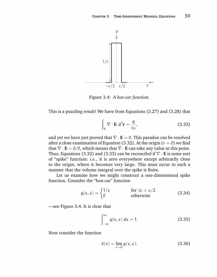
“chapter3” — 2007/12/14 — 12:02 — page 59 — #11
CHAPTER 3 TIME-INDEPENDENT MAXWELL EQUATIONS 59
−ε/2 xε/2
1/ε
g
Figure 3.4: A box-car function.
This is a puzzling result! We have from Equations (3.27) and (3.28) that∫V
∇ · E d3r =q
ε0, (3.33)
and yet we have just proved that ∇ · E = 0. This paradox can be resolvedafter a close examination of Equation (3.32). At the origin (r = 0) we findthat ∇ · E = 0/0, which means that ∇ · E can take any value at this point.Thus, Equations (3.32) and (3.33) can be reconciled if ∇ · E is some sortof “spike” function: i.e., it is zero everywhere except arbitrarily closeto the origin, where it becomes very large. This must occur in such amanner that the volume integral over the spike is finite.
Let us examine how we might construct a one-dimensional spikefunction. Consider the “box-car” function
g(x, ε) =
1/ε for |x| < ε/2
0 otherwise (3.34)
—see Figure 3.4. It is clear that∫
∞
−∞
g(x, ε)dx = 1. (3.35)
Now consider the function
δ(x) = limε→0
g(x, ε). (3.36)
“chapter3” — 2007/12/14 — 12:02 — page 60 — #12
60 MAXWELL’S EQUATIONS AND THE PRINCIPLES OF ELECTROMAGNETISM
This is zero everywhere except arbitrarily close to x = 0. According toEquation (3.35), it also possess a finite integral;∫
∞
−∞
δ(x)dx = 1. (3.37)
Thus, δ(x) has all of the required properties of a spike function. Theone-dimensional spike function δ(x) is called the Dirac delta-function,after the Cambridge physicist Paul Dirac who invented it in 1927 whilstinvestigating Quantum Mechanics. The delta-function is an example ofwhat mathematicians call a generalized function: it is not well-defined atx = 0, but its integral is nevertheless well-defined. Consider the integral∫
∞
−∞
f(x) δ(x)dx, (3.38)
where f(x) is a function which is well-behaved in the vicinity of x = 0.Since the delta-function is zero everywhere apart from very close tox = 0, it is clear that∫
∞
−∞
f(x) δ(x)dx = f(0)
∫∞
−∞
δ(x)dx = f(0), (3.39)
where use has been made of Equation (3.37). The above equation, whichis valid for any well-behaved function, f(x), is effectively the definition ofa delta-function. A simple change of variables allows us to define δ(x−x0), which is a spike function centered on x = x0. Equation (3.39) gives∫
∞
−∞
f(x) δ(x− x0)dx = f(x0). (3.40)
We actually want a three-dimensional spike function: i.e., a functionwhich is zero everywhere apart from arbitrarily close to the origin, andwhose volume integral is unity. If we denote this function by δ(r) thenit is easily seen that the three-dimensional delta-function is the productof three one-dimensional delta-functions:
δ(r) = δ(x) δ(y) δ(z). (3.41)
This function is clearly zero everywhere except the origin. But is itsvolume integral unity? Let us integrate over a cube of dimension 2 awhich is centered on the origin, and aligned along the Cartesian axes.This volume integral is obviously separable, so that∫
δ(r)d3r =
∫a−a
δ(x)dx
∫a−a
δ(y)dy
∫a−a
δ(z)dz. (3.42)
“chapter3” — 2007/12/14 — 12:02 — page 61 — #13
CHAPTER 3 TIME-INDEPENDENT MAXWELL EQUATIONS 61
The integral can be turned into an integral over all space by takingthe limit a → ∞. However, we know that for one-dimensional delta-functions
∫∞
−∞δ(x)dx = 1, so it follows from the above equation that∫
δ(r)d3r = 1, (3.43)
which is the desired result. A simple generalization of previous argu-ments yields ∫
f(r) δ(r)d3r = f(0), (3.44)
where f(r) is any well-behaved scalar field. Finally, we can changevariables and write
δ(r − r ′) = δ(x− x ′) δ(y− y ′) δ(z− z ′), (3.45)
which is a three-dimensional spike function centered on r = r ′. It is easilydemonstrated that ∫
f(r) δ(r − r ′)d3r = f(r ′). (3.46)
Up to now, we have only considered volume integrals taken over allspace. However, it should be obvious that the above result also holdsfor integrals over any finite volume V which contains the point r = r ′.Likewise, the integral is zero if V does not contain r = r ′.
Let us now return to the problem in hand. The electric field generatedby a charge q located at the origin has ∇ · E = 0 everywhere apart fromthe origin, and also satisfies∫
V
∇ · E d3r =q
ε0(3.47)
for a spherical volume V centered on the origin. These two facts implythat
∇ · E =q
ε0δ(r), (3.48)
where use has been made of Equation (3.43).At this stage, vector field theory has yet to show its worth. After all,
we have just spent an inordinately long time proving something usingvector field theory which we previously proved in one line [see Equa-tion (3.27)] using conventional analysis. It is time to demonstrate the
“chapter3” — 2007/12/14 — 12:02 — page 62 — #14
62 MAXWELL’S EQUATIONS AND THE PRINCIPLES OF ELECTROMAGNETISM
power of vector field theory. Consider, again, a charge q at the origin sur-rounded by a spherical surface Swhich is centered on the origin. Supposethat we now displace the surface S, so that it is no longer centered on theorigin. What is the flux of the electric field out of S? This is no longer asimple problem for conventional analysis, because the normal to the sur-face is not parallel to the local electric field. However, using vector fieldtheory this problem is no more difficult than the previous one. We have∮
S
E · dS =
∫V
∇ · E d3r (3.49)
from Gauss’ theorem, plus Equation (3.48). From these equations, it isclear that the flux of E out of S is q/ε0 for a spherical surface displacedfrom the origin. However, the flux becomes zero when the displacementis sufficiently large that the origin is no longer enclosed by the sphere.It is possible to prove this via conventional analysis, but it is certainlynot easy. Suppose that the surface S is not spherical but is instead highlydistorted. What now is the flux of E out of S? This is a virtually impossi-ble problem in conventional analysis, but it is still easy using vector fieldtheory. Gauss’ theorem and Equation (3.48) tell us that the flux is q/ε0provided that the surface contains the origin, and that the flux is zerootherwise. This result is completely independent of the shape of S.
Consider N charges qi located at ri. A simple generalization ofEquation (3.48) gives
∇ · E =
N∑i=1
qi
ε0δ(r − ri). (3.50)
Thus, Gauss’ theorem (3.49) implies that∮S
E · dS =
∫V
∇ · E d3r =Q
ε0, (3.51)
whereQ is the total charge enclosed by the surface S. This result is calledGauss’ law, and does not depend on the shape of the surface.
Suppose, finally, that instead of having a set of discrete charges, wehave a continuous charge distribution described by a charge density ρ(r).The charge contained in a small rectangular volume of dimensions dx,dy, and dz located at position r is Q = ρ(r)dxdydz. However, if weintegrate ∇ · E over this volume element we obtain
∇ · E dxdydz =Q
ε0=ρdxdydz
ε0, (3.52)
“chapter3” — 2007/12/14 — 12:02 — page 63 — #15
CHAPTER 3 TIME-INDEPENDENT MAXWELL EQUATIONS 63
where use has been made of Equation (3.51). Here, the volume elementis assumed to be sufficiently small that ∇ · E does not vary significantlyacross it. Thus, we get
∇ · E =ρ
ε0. (3.53)
This is the first of four field equations, called Maxwell’s equations, whichtogether form a complete description of electromagnetism. Of course,our derivation of Equation (3.53) is only valid for electric fields generatedby stationary charge distributions. In principle, additional terms mightbe required to describe fields generated by moving charge distributions.However, it turns out that this is not the case, and that Equation (3.53)is universally valid.
Equation (3.53) is a differential equation describing the electric fieldgenerated by a set of charges. We already know the solution to thisequation when the charges are stationary: it is given by Equation (3.12),
E(r) =1
4πε0
∫ρ(r ′)
r − r ′
|r − r ′|3d3r ′. (3.54)
Equations (3.53) and (3.54) can be reconciled provided
∇ ·(
r − r ′
|r − r ′|3
)= −∇2
(1
|r − r ′|
)= 4π δ(r − r ′), (3.55)
where use has been made of Equation (3.15). It follows that
∇ · E(r) =1
4πε0
∫ρ(r ′)∇ ·
(r − r ′
|r − r ′|3
)d3r ′
=
∫ρ(r ′)ε0
δ(r − r ′)d3r ′ =ρ(r)ε0, (3.56)
which is the desired result. The most general form of Gauss’ law, Equa-tion (3.51), is obtained by integrating Equation (3.53) over a volume Vsurrounded by a surface S, and making use of Gauss’ theorem:∮
S
E · dS =1
ε0
∫V
ρ(r)d3r. (3.57)
One particularly interesting application of Gauss’ law is Earnshaw’stheorem, which states that it is impossible for a collection of chargedparticles to remain in static equilibrium solely under the influence of
“chapter3” — 2007/12/14 — 12:02 — page 64 — #16
64 MAXWELL’S EQUATIONS AND THE PRINCIPLES OF ELECTROMAGNETISM
(classical) electrostatic forces. For instance, consider the motion of theith particle in the electric field, E(r), generated by all of the other staticparticles. The equilibrium position of the ith particle corresponds to somepoint ri, where E(ri) = 0. By implication, ri does not correspond to theequilibrium position of any other particle. However, in order for ri to bea stable equilibrium point, the particle must experience a restoring forcewhen it moves a small distance away from ri in any direction. Assumingthat the ith particle is positively charged, this means that the electricfield must point radially toward ri at all neighboring points. Hence, ifwe apply Gauss’ law to a small sphere centered on ri then there mustbe a negative flux of E through the surface of the sphere, implying thepresence of a negative charge at ri. However, there is no such chargeat ri. Hence, we conclude that E cannot point radially toward ri at allneighboring points. In other words, there must be some neighboringpoints at which E is directed away from ri. Hence, a positively chargedparticle placed at ri can always escape by moving to such points. Onecorollary of Earnshaw’s theorem is that classical electrostatics cannotaccount for the stability of atoms and molecules.
As an example of the use of Gauss’ law, let us calculate the elec-tric field generated by a spherically symmetric charge annulus of innerradius a, and outer radius b, centered on the origin, and carrying auniformly distributed chargeQ. Now, from symmetry, we expect a spher-ically symmetric charge distribution to generate a spherically symmetricpotential, φ(r). It therefore follows that the electric field is both spheri-cally symmetric and radial: i.e., E = Er(r) er. Let us apply Gauss’ law toan imaginary spherical surface, of radius r, centered on the origin—seeFigure 3.5. Such a surface is generally known as a Gaussian surface. Now,according to Gauss’ law, the flux of the electric field out of the surfaceis equal to the enclosed charge, divided by ε0. The flux is easy to calcu-late since the electric field is everywhere perpendicular to the surface.We obtain
4π r2 Er(r) =Q(r)
ε0,
where Q(r) is the charge enclosed by a Gaussian surface of radius r.Now, it is evident that
Q(r) =
0 r < a
[(r3 − a3)/(b3 − a3)]Q a ≤ r ≤ b
Q b < r
. (3.58)
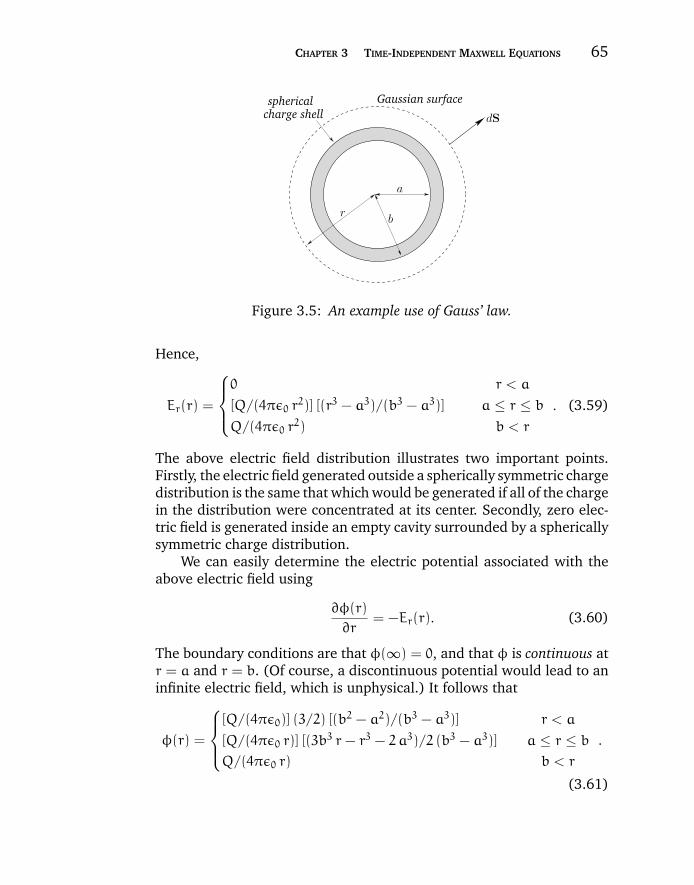
“chapter3” — 2007/12/14 — 12:02 — page 65 — #17
CHAPTER 3 TIME-INDEPENDENT MAXWELL EQUATIONS 65
a
br
dS
sphericalcharge shell
Gaussian surface
Figure 3.5: An example use of Gauss’ law.
Hence,
Er(r) =
0 r < a
[Q/(4πε0 r2)] [(r3 − a3)/(b3 − a3)] a ≤ r ≤ b
Q/(4πε0 r2) b < r
. (3.59)
The above electric field distribution illustrates two important points.Firstly, the electric field generated outside a spherically symmetric chargedistribution is the same that which would be generated if all of the chargein the distribution were concentrated at its center. Secondly, zero elec-tric field is generated inside an empty cavity surrounded by a sphericallysymmetric charge distribution.
We can easily determine the electric potential associated with theabove electric field using
∂φ(r)
∂r= −Er(r). (3.60)
The boundary conditions are that φ(∞) = 0, and that φ is continuous atr = a and r = b. (Of course, a discontinuous potential would lead to aninfinite electric field, which is unphysical.) It follows that
φ(r) =
[Q/(4πε0)] (3/2) [(b2 − a2)/(b3 − a3)] r < a
[Q/(4πε0 r)] [(3b3 r− r3 − 2 a3)/2 (b3 − a3)] a ≤ r ≤ b
Q/(4πε0 r) b < r
.
(3.61)
“chapter3” — 2007/12/14 — 12:02 — page 66 — #18
66 MAXWELL’S EQUATIONS AND THE PRINCIPLES OF ELECTROMAGNETISM
Hence, the work done in slowly moving a charge from infinity to thecenter of the distribution (which is minus the work done by the electricfield) is
W = q [φ(0) − φ(∞)] =qQ
4πε0
3
2
(b2 − a2
b3 − a3
). (3.62)
3.5 POISSON’S EQUATION
We have seen that the electric field generated by a set of stationarycharges can be written as the gradient of a scalar potential, so that
E = −∇φ. (3.63)
This equation can be combined with the field equation (3.53) to give apartial differential equation for the scalar potential:
∇2φ = −ρ
ε0. (3.64)
This is an example of a very famous type of partial differential equationknown as Poisson’s equation.
In its most general form, Poisson’s equation is written
∇2u = v, (3.65)
where u(r) is some scalar potential which is to be determined, and v(r)is a known “source function.” The most common boundary conditionapplied to this equation is that the potential u is zero at infinity. Thesolutions to Poisson’s equation are completely superposable. Thus, ifu1 is the potential generated by the source function v1, and u2 is thepotential generated by the source function v2, so that
∇2u1 = v1, ∇2u2 = v2, (3.66)
then the potential generated by v1 + v2 is u1 + u2, since
∇2(u1 + u2) = ∇2u1 + ∇2u2 = v1 + v2. (3.67)
Poisson’s equation has this property because it is linear in both thepotential and the source term.
The fact that the solutions to Poisson’s equation are superposablesuggests a general method for solving this equation. Suppose that we

“chapter3” — 2007/12/14 — 12:02 — page 67 — #19
CHAPTER 3 TIME-INDEPENDENT MAXWELL EQUATIONS 67
could construct all of the solutions generated by point sources. Of course,these solutions must satisfy the appropriate boundary conditions. Anygeneral source function can be built up out of a set of suitably weightedpoint sources, so the general solution of Poisson’s equation must beexpressible as a similarly weighted sum over the point source solutions.Thus, once we know all of the point source solutions we can construct anyother solution. In mathematical terminology, we require the solution to
∇2G(r, r ′) = δ(r − r ′) (3.68)
which goes to zero as |r| → ∞. The function G(r, r ′) is the solution gen-erated by a unit point source located at position r ′. This function isknown to mathematicians as a Green’s function. The solution generatedby a general source function v(r) is simply the appropriately weightedsum of all of the Green’s function solutions:
u(r) =
∫G(r, r ′) v(r ′)d3r ′. (3.69)
We can easily demonstrate that this is the correct solution:
∇2u(r) =
∫ [∇2G(r, r ′)
]v(r ′)d3r ′ =
∫δ(r − r ′) v(r ′)d3r ′ = v(r).
(3.70)
Let us return to Equation (3.64):
∇2φ = −ρ
ε0. (3.71)
The Green’s function for this equation satisfies Equation (3.68) with|G| → ∞ as |r| → 0. It follows from Equation (3.55) that
G(r, r ′) = −1
4π
1
|r − r ′|. (3.72)
Note, from Equation (3.20), that the Green’s function has the same formas the potential generated by a point charge. This is hardly surprising,given the definition of a Green’s function. It follows from Equation (3.69)and (3.72) that the general solution to Poisson’s equation, (3.71), iswritten
φ(r) =1
4πε0
∫ρ(r ′)
|r − r ′|d3r ′. (3.73)
In fact, we have already obtained this solution by another method [seeEquation (3.17)].
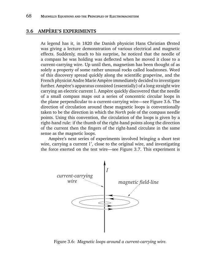
“chapter3” — 2007/12/14 — 12:02 — page 68 — #20
68 MAXWELL’S EQUATIONS AND THE PRINCIPLES OF ELECTROMAGNETISM
3.6 AMPERE’S EXPERIMENTS
As legend has it, in 1820 the Danish physicist Hans Christian Ørstedwas giving a lecture demonstration of various electrical and magneticeffects. Suddenly, much to his surprise, he noticed that the needle ofa compass he was holding was deflected when he moved it close to acurrent-carrying wire. Up until then, magnetism has been thought of assolely a property of some rather unusual rocks called loadstones. Wordof this discovery spread quickly along the scientific grapevine, and theFrench physicist Andre Marie Ampere immediately decided to investigatefurther. Ampere’s apparatus consisted (essentially) of a long straight wirecarrying an electric current I. Ampere quickly discovered that the needleof a small compass maps out a series of concentric circular loops inthe plane perpendicular to a current-carrying wire—see Figure 3.6. Thedirection of circulation around these magnetic loops is conventionallytaken to be the direction in which the North pole of the compass needlepoints. Using this convention, the circulation of the loops is given by aright-hand rule: if the thumb of the right-hand points along the directionof the current then the fingers of the right-hand circulate in the samesense as the magnetic loops.
Ampere’s next series of experiments involved bringing a short testwire, carrying a current I ′, close to the original wire, and investigatingthe force exerted on the test wire—see Figure 3.7. This experiment is
magnetic field-linewire
Icurrent-carrying
Figure 3.6: Magnetic loops around a current-carrying wire.
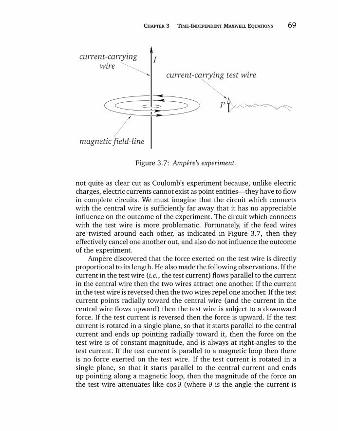
“chapter3” — 2007/12/14 — 12:02 — page 69 — #21
CHAPTER 3 TIME-INDEPENDENT MAXWELL EQUATIONS 69
wire
I ′
I
current-carrying test wire
magnetic field-line
current-carrying
Figure 3.7: Ampere’s experiment.
not quite as clear cut as Coulomb’s experiment because, unlike electriccharges, electric currents cannot exist as point entities—they have to flowin complete circuits. We must imagine that the circuit which connectswith the central wire is sufficiently far away that it has no appreciableinfluence on the outcome of the experiment. The circuit which connectswith the test wire is more problematic. Fortunately, if the feed wiresare twisted around each other, as indicated in Figure 3.7, then theyeffectively cancel one another out, and also do not influence the outcomeof the experiment.
Ampere discovered that the force exerted on the test wire is directlyproportional to its length. He also made the following observations. If thecurrent in the test wire (i.e., the test current) flows parallel to the currentin the central wire then the two wires attract one another. If the currentin the test wire is reversed then the two wires repel one another. If the testcurrent points radially toward the central wire (and the current in thecentral wire flows upward) then the test wire is subject to a downwardforce. If the test current is reversed then the force is upward. If the testcurrent is rotated in a single plane, so that it starts parallel to the centralcurrent and ends up pointing radially toward it, then the force on thetest wire is of constant magnitude, and is always at right-angles to thetest current. If the test current is parallel to a magnetic loop then thereis no force exerted on the test wire. If the test current is rotated in asingle plane, so that it starts parallel to the central current and endsup pointing along a magnetic loop, then the magnitude of the force onthe test wire attenuates like cos θ (where θ is the angle the current is
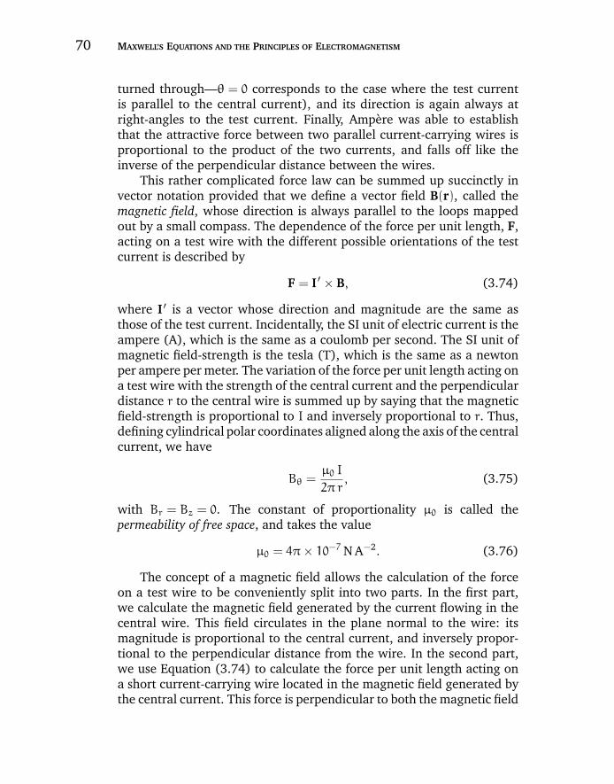
“chapter3” — 2007/12/14 — 12:02 — page 70 — #22
70 MAXWELL’S EQUATIONS AND THE PRINCIPLES OF ELECTROMAGNETISM
turned through—θ = 0 corresponds to the case where the test currentis parallel to the central current), and its direction is again always atright-angles to the test current. Finally, Ampere was able to establishthat the attractive force between two parallel current-carrying wires isproportional to the product of the two currents, and falls off like theinverse of the perpendicular distance between the wires.
This rather complicated force law can be summed up succinctly invector notation provided that we define a vector field B(r), called themagnetic field, whose direction is always parallel to the loops mappedout by a small compass. The dependence of the force per unit length, F,acting on a test wire with the different possible orientations of the testcurrent is described by
F = I ′ × B, (3.74)
where I ′ is a vector whose direction and magnitude are the same asthose of the test current. Incidentally, the SI unit of electric current is theampere (A), which is the same as a coulomb per second. The SI unit ofmagnetic field-strength is the tesla (T), which is the same as a newtonper ampere per meter. The variation of the force per unit length acting ona test wire with the strength of the central current and the perpendiculardistance r to the central wire is summed up by saying that the magneticfield-strength is proportional to I and inversely proportional to r. Thus,defining cylindrical polar coordinates aligned along the axis of the centralcurrent, we have
Bθ =µ0 I
2π r, (3.75)
with Br = Bz = 0. The constant of proportionality µ0 is called thepermeability of free space, and takes the value
µ0 = 4π× 10−7 N A−2. (3.76)
The concept of a magnetic field allows the calculation of the forceon a test wire to be conveniently split into two parts. In the first part,we calculate the magnetic field generated by the current flowing in thecentral wire. This field circulates in the plane normal to the wire: itsmagnitude is proportional to the central current, and inversely propor-tional to the perpendicular distance from the wire. In the second part,we use Equation (3.74) to calculate the force per unit length acting ona short current-carrying wire located in the magnetic field generated bythe central current. This force is perpendicular to both the magnetic field
“chapter3” — 2007/12/14 — 12:02 — page 71 — #23
CHAPTER 3 TIME-INDEPENDENT MAXWELL EQUATIONS 71
and the direction of the test current. Note that, at this stage, we have noreason to suppose that the magnetic field has any real physical existence.It is introduced merely to facilitate the calculation of the force exertedon the test wire by the central wire.
3.7 THE LORENTZ FORCE
The flow of an electric current down a conducting wire is ultimately dueto the motion of electrically charged particles (in most cases, electrons)through the conducting medium. It seems reasonable, therefore, thatthe force exerted on the wire when it is placed in a magnetic field isreally the resultant of the forces exerted on these moving charges. Letus suppose that this is the case.
Let A be the (uniform) cross-sectional area of the (cylindrical) wire,and let n be the number density of mobile charges in the conductor.Suppose that the mobile charges each have charge q and velocity v.We must assume that the conductor also contains stationary charges, ofcharge −q and number density n (say), so that the net charge density inthe wire is zero. In most conductors, the mobile charges are electrons,and the stationary charges are ions. The magnitude of the electric currentflowing through the wire is simply the number of coulombs per secondwhich flow past a given point. In one second, a mobile charge moves adistance v, so all of the charges contained in a cylinder of cross-sectionalarea A and length v flow past a given point. Thus, the magnitude of thecurrent is qnAv. The direction of the current is the same as the directionof motion of the charges, so the vector current is I ′ = qnA v. Accordingto Equation (3.74), the force per unit length acting on the wire is
F = qnA v × B. (3.77)
However, a unit length of the wire contains nA moving charges. So,assuming that each charge is subject to an equal force from the mag-netic field (we have no reason to suppose otherwise), the force actingon an individual charge is
f = q v × B. (3.78)
We can combine this with Equation (3.9) to give the force acting on acharge q moving with velocity v in an electric field E and a magneticfield B:
f = qE + q v × B. (3.79)

“chapter3” — 2007/12/14 — 12:02 — page 72 — #24
72 MAXWELL’S EQUATIONS AND THE PRINCIPLES OF ELECTROMAGNETISM
This is called the Lorentz force law, after the Dutch physicist HendrikAntoon Lorentz who first formulated it. The electric force on a chargedparticle is parallel to the local electric field. The magnetic force, how-ever, is perpendicular to both the local magnetic field and the particle’sdirection of motion. No magnetic force is exerted on a stationary chargedparticle.
The equation of motion of a free particle of charge q and mass mmoving in electric and magnetic fields is
mdvdt
= qE + q v × B, (3.80)
according to the Lorentz force law. This equation of motion was firstverified in a famous experiment carried out by the Cambridge physicistJ.J. Thompson in 1897. Thompson was investigating cathode rays, a thenmysterious form of radiation emitted by a heated metal element held ata large negative voltage (i.e., a cathode) with respect to another metalelement (i.e., an anode) in an evacuated tube. German physicists heldthat cathode rays were a form of electromagnetic radiation, whilst Britishand French physicists suspected that they were, in reality, a stream ofcharged particles. Thompson was able to demonstrate that the latter viewwas correct. In Thompson’s experiment, the cathode rays passed thougha region of “crossed” electric and magnetic fields (still in vacuum). Thefields were perpendicular to the original trajectory of the rays, and werealso mutually perpendicular.
Let us analyze Thompson’s experiment. Suppose that the rays areoriginally traveling in the x-direction, and are subject to a uniform elec-tric field E in the z-direction and a uniform magnetic field B in the−y-direction—see Figure 3.8. Let us assume, as Thompson did, thatcathode rays are a stream of particles of mass m and charge q. Theequation of motion of the particles in the z-direction is
md2z
dt2= q (E− vB) , (3.81)
where v is the velocity of the particles in the x-direction. Thompsonstarted off his experiment by only turning on the electric field in hisapparatus, and measuring the deflection d of the ray in the z-directionafter it had traveled a distance l through the electric field. It is clear fromthe equation of motion that
d =q
m
E t2
2=q
m
E l2
2 v2, (3.82)
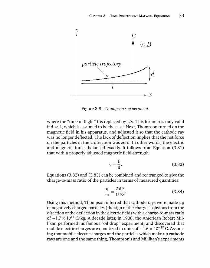
“chapter3” — 2007/12/14 — 12:02 — page 73 — #25
CHAPTER 3 TIME-INDEPENDENT MAXWELL EQUATIONS 73
particle trajectory
B
lx
z
d
E
Figure 3.8: Thompson’s experiment.
where the “time of flight” t is replaced by l/v. This formula is only validif d l, which is assumed to be the case. Next, Thompson turned on themagnetic field in his apparatus, and adjusted it so that the cathode raywas no longer deflected. The lack of deflection implies that the net forceon the particles in the z-direction was zero. In other words, the electricand magnetic forces balanced exactly. It follows from Equation (3.81)that with a properly adjusted magnetic field-strength
v =E
B. (3.83)
Equations (3.82) and (3.83) can be combined and rearranged to give thecharge-to-mass ratio of the particles in terms of measured quantities:
q
m=2 dE
l2 B2. (3.84)
Using this method, Thompson inferred that cathode rays were made upof negatively charged particles (the sign of the charge is obvious from thedirection of the deflection in the electric field) with a charge-to-mass ratioof −1.7× 10¹¹ C/kg. A decade later, in 1908, the American Robert Mil-likan performed his famous “oil drop” experiment, and discovered thatmobile electric charges are quantized in units of −1.6× 10⁻¹⁹ C. Assum-ing that mobile electric charges and the particles which make up cathoderays are one and the same thing, Thompson’s and Millikan’s experiments
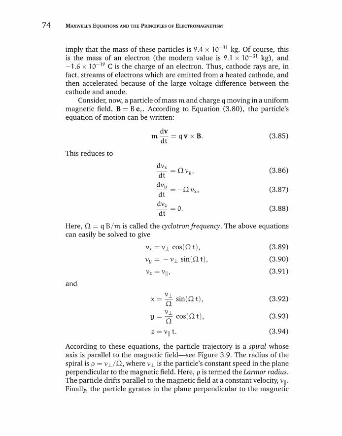
“chapter3” — 2007/12/14 — 12:02 — page 74 — #26
74 MAXWELL’S EQUATIONS AND THE PRINCIPLES OF ELECTROMAGNETISM
imply that the mass of these particles is 9.4× 10⁻³¹ kg. Of course, thisis the mass of an electron (the modern value is 9.1× 10⁻³¹ kg), and−1.6× 10⁻¹⁹ C is the charge of an electron. Thus, cathode rays are, infact, streams of electrons which are emitted from a heated cathode, andthen accelerated because of the large voltage difference between thecathode and anode.
Consider, now, a particle of massm and chargeqmoving in a uniformmagnetic field, B = B ez. According to Equation (3.80), the particle’sequation of motion can be written:
mdvdt
= q v × B. (3.85)
This reduces to
dvx
dt= Ωvy, (3.86)
dvy
dt= −Ωvx, (3.87)
dvz
dt= 0. (3.88)
Here, Ω = qB/m is called the cyclotron frequency. The above equationscan easily be solved to give
vx = v⊥ cos(Ωt), (3.89)
vy = − v⊥ sin(Ωt), (3.90)
vz = v‖, (3.91)
and
x =v⊥Ω
sin(Ωt), (3.92)
y =v⊥Ω
cos(Ωt), (3.93)
z = v‖ t. (3.94)
According to these equations, the particle trajectory is a spiral whoseaxis is parallel to the magnetic field—see Figure 3.9. The radius of thespiral is ρ = v⊥/Ω, where v⊥ is the particle’s constant speed in the planeperpendicular to the magnetic field. Here, ρ is termed the Larmor radius.The particle drifts parallel to the magnetic field at a constant velocity, v‖.Finally, the particle gyrates in the plane perpendicular to the magnetic
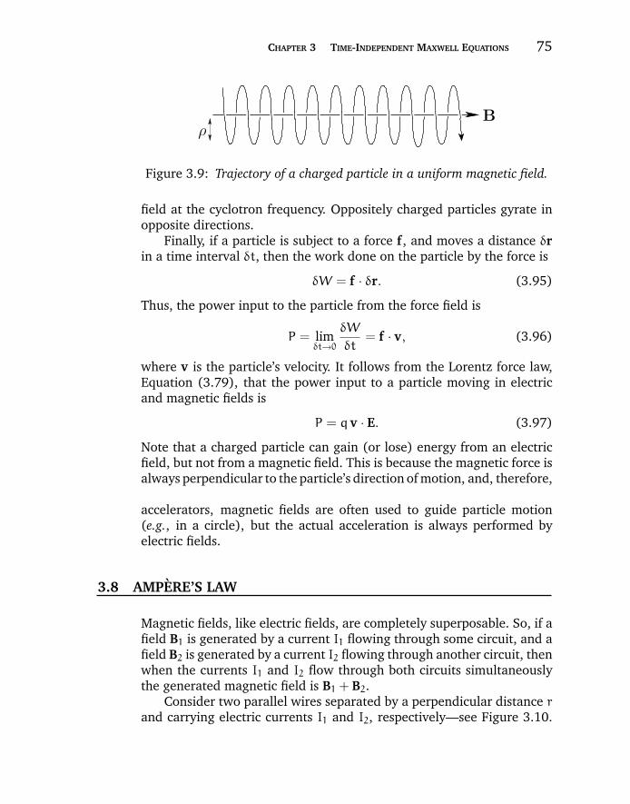
“chapter3” — 2007/12/14 — 12:02 — page 75 — #27
CHAPTER 3 TIME-INDEPENDENT MAXWELL EQUATIONS 75
ρB
Figure 3.9: Trajectory of a charged particle in a uniform magnetic field.
field at the cyclotron frequency. Oppositely charged particles gyrate inopposite directions.
Finally, if a particle is subject to a force f , and moves a distance δrin a time interval δt, then the work done on the particle by the force is
δW = f · δr. (3.95)
Thus, the power input to the particle from the force field is
P = limδt→0
δW
δt= f · v, (3.96)
where v is the particle’s velocity. It follows from the Lorentz force law,Equation (3.79), that the power input to a particle moving in electricand magnetic fields is
P = q v · E. (3.97)
Note that a charged particle can gain (or lose) energy from an electricfield, but not from a magnetic field. This is because the magnetic force isalways perpendicular to the particle’s direction of motion, and, therefore,does no work on the particle [see Equation (3.95)]. Thus, in particleaccelerators, magnetic fields are often used to guide particle motion(e.g., in a circle), but the actual acceleration is always performed byelectric fields.
3.8 AMPERE’S LAW
Magnetic fields, like electric fields, are completely superposable. So, if afield B1 is generated by a current I1 flowing through some circuit, and afield B2 is generated by a current I2 flowing through another circuit, thenwhen the currents I1 and I2 flow through both circuits simultaneouslythe generated magnetic field is B1 + B2.
Consider two parallel wires separated by a perpendicular distance rand carrying electric currents I1 and I2, respectively—see Figure 3.10.
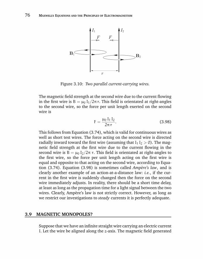
“chapter3” — 2007/12/14 — 12:02 — page 76 — #28
76 MAXWELL’S EQUATIONS AND THE PRINCIPLES OF ELECTROMAGNETISM
FF
I1 I2
B1 B2
r
Figure 3.10: Two parallel current-carrying wires.
The magnetic field strength at the second wire due to the current flowingin the first wire is B = µ0 I1/2π r. This field is orientated at right-anglesto the second wire, so the force per unit length exerted on the secondwire is
F =µ0 I1 I2
2π r. (3.98)
This follows from Equation (3.74), which is valid for continuous wires aswell as short test wires. The force acting on the second wire is directedradially inward toward the first wire (assuming that I1 I2 > 0). The mag-netic field strength at the first wire due to the current flowing in thesecond wire is B = µ0 I2/2π r. This field is orientated at right-angles tothe first wire, so the force per unit length acting on the first wire isequal and opposite to that acting on the second wire, according to Equa-tion (3.74). Equation (3.98) is sometimes called Ampere’s law, and isclearly another example of an action-at-a-distance law: i.e., if the cur-rent in the first wire is suddenly changed then the force on the secondwire immediately adjusts. In reality, there should be a short time delay,at least as long as the propagation time for a light signal between the twowires. Clearly, Ampere’s law is not strictly correct. However, as long aswe restrict our investigations to steady currents it is perfectly adequate.
3.9 MAGNETIC MONOPOLES?
Suppose that we have an infinite straight wire carrying an electric currentI. Let the wire be aligned along the z-axis. The magnetic field generated
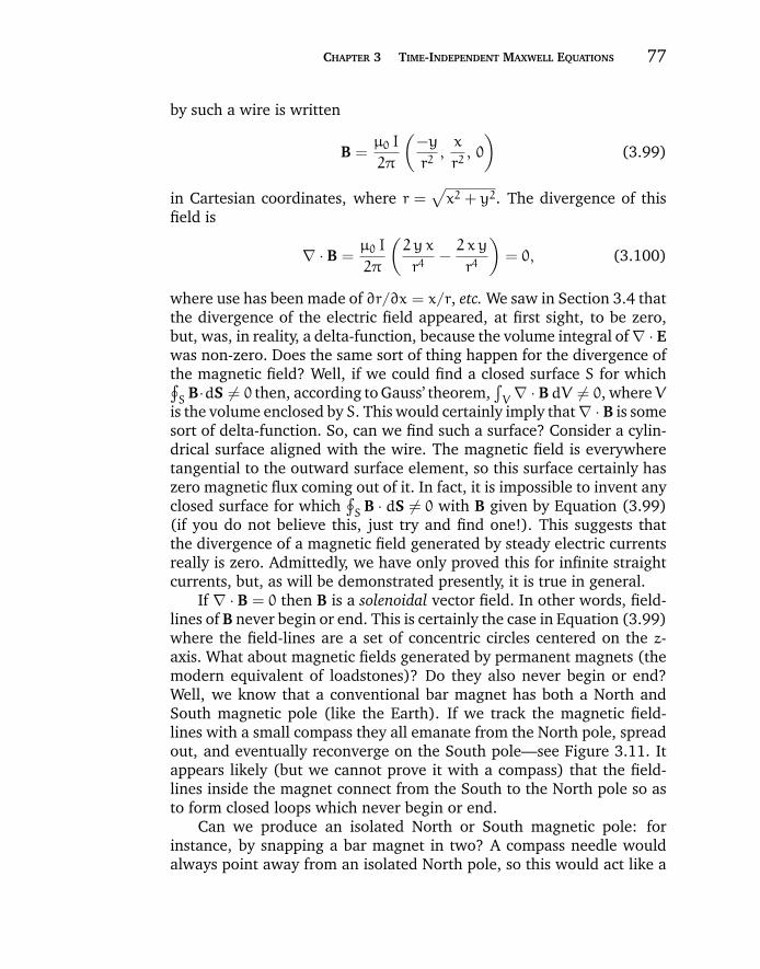
“chapter3” — 2007/12/14 — 12:02 — page 77 — #29
CHAPTER 3 TIME-INDEPENDENT MAXWELL EQUATIONS 77
by such a wire is written
B =µ0 I
2π
(−y
r2,x
r2, 0
)(3.99)
in Cartesian coordinates, where r =√x2 + y2. The divergence of this
field is
∇ · B =µ0 I
2π
(2 y x
r4−2 x y
r4
)= 0, (3.100)
where use has been made of ∂r/∂x = x/r, etc. We saw in Section 3.4 thatthe divergence of the electric field appeared, at first sight, to be zero,but, was, in reality, a delta-function, because the volume integral of ∇ · Ewas non-zero. Does the same sort of thing happen for the divergence ofthe magnetic field? Well, if we could find a closed surface S for which∮S
B·dS = 0 then, according to Gauss’ theorem,∫V
∇ · BdV = 0, whereVis the volume enclosed by S. This would certainly imply that ∇ · B is somesort of delta-function. So, can we find such a surface? Consider a cylin-drical surface aligned with the wire. The magnetic field is everywheretangential to the outward surface element, so this surface certainly haszero magnetic flux coming out of it. In fact, it is impossible to invent anyclosed surface for which
∮S
B · dS = 0 with B given by Equation (3.99)(if you do not believe this, just try and find one!). This suggests thatthe divergence of a magnetic field generated by steady electric currentsreally is zero. Admittedly, we have only proved this for infinite straightcurrents, but, as will be demonstrated presently, it is true in general.
If ∇ · B = 0 then B is a solenoidal vector field. In other words, field-lines of B never begin or end. This is certainly the case in Equation (3.99)where the field-lines are a set of concentric circles centered on the z-axis. What about magnetic fields generated by permanent magnets (themodern equivalent of loadstones)? Do they also never begin or end?Well, we know that a conventional bar magnet has both a North andSouth magnetic pole (like the Earth). If we track the magnetic field-lines with a small compass they all emanate from the North pole, spreadout, and eventually reconverge on the South pole—see Figure 3.11. Itappears likely (but we cannot prove it with a compass) that the field-lines inside the magnet connect from the South to the North pole so asto form closed loops which never begin or end.
Can we produce an isolated North or South magnetic pole: forinstance, by snapping a bar magnet in two? A compass needle wouldalways point away from an isolated North pole, so this would act like a
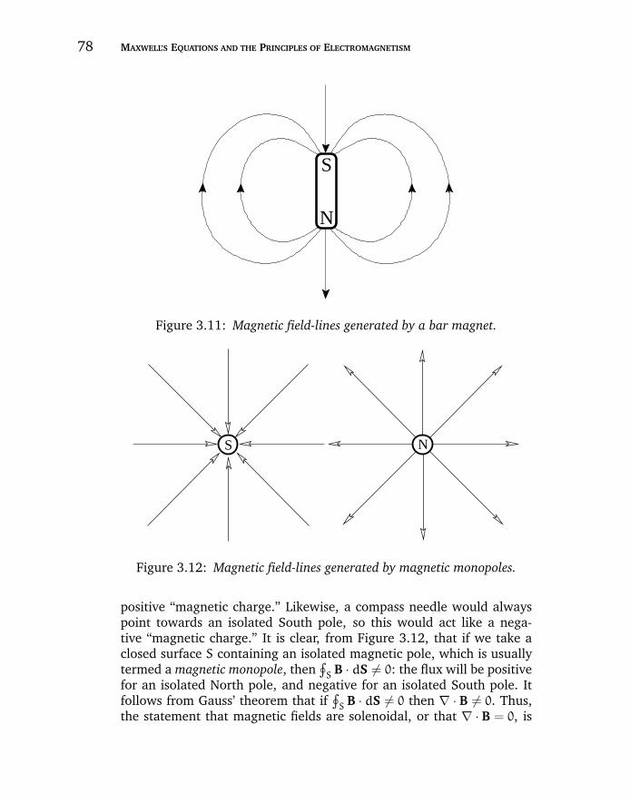
“chapter3” — 2007/12/14 — 12:02 — page 78 — #30
78 MAXWELL’S EQUATIONS AND THE PRINCIPLES OF ELECTROMAGNETISM
S
N
Figure 3.11: Magnetic field-lines generated by a bar magnet.
S N
Figure 3.12: Magnetic field-lines generated by magnetic monopoles.
positive “magnetic charge.” Likewise, a compass needle would alwayspoint towards an isolated South pole, so this would act like a nega-tive “magnetic charge.” It is clear, from Figure 3.12, that if we take aclosed surface S containing an isolated magnetic pole, which is usuallytermed a magnetic monopole, then
∮S
B · dS = 0: the flux will be positivefor an isolated North pole, and negative for an isolated South pole. Itfollows from Gauss’ theorem that if
∮S
B · dS = 0 then ∇ · B = 0. Thus,the statement that magnetic fields are solenoidal, or that ∇ · B = 0, is
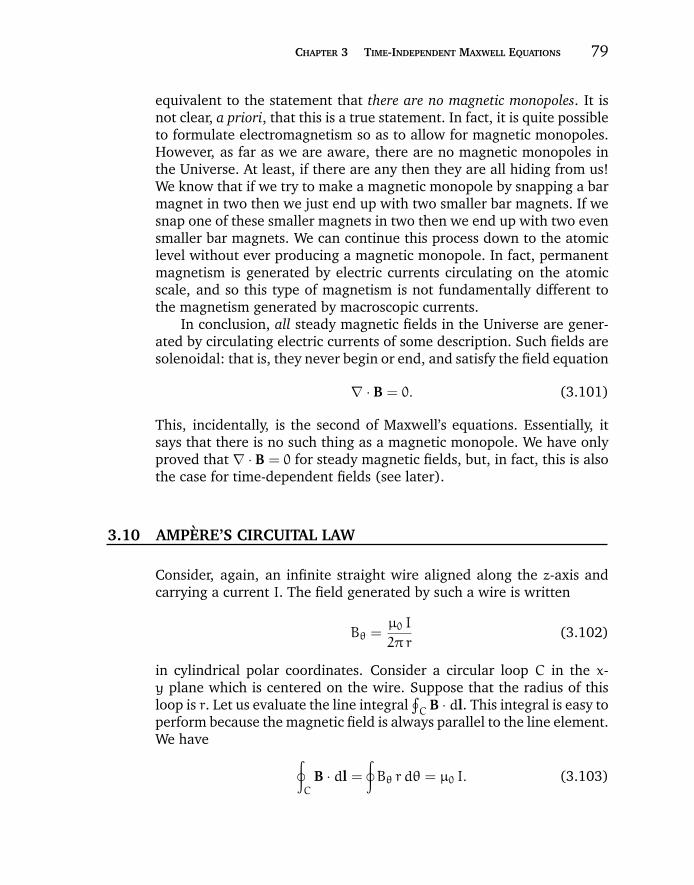
“chapter3” — 2007/12/14 — 12:02 — page 79 — #31
CHAPTER 3 TIME-INDEPENDENT MAXWELL EQUATIONS 79
equivalent to the statement that there are no magnetic monopoles. It isnot clear, a priori, that this is a true statement. In fact, it is quite possibleto formulate electromagnetism so as to allow for magnetic monopoles.However, as far as we are aware, there are no magnetic monopoles inthe Universe. At least, if there are any then they are all hiding from us!We know that if we try to make a magnetic monopole by snapping a barmagnet in two then we just end up with two smaller bar magnets. If wesnap one of these smaller magnets in two then we end up with two evensmaller bar magnets. We can continue this process down to the atomiclevel without ever producing a magnetic monopole. In fact, permanentmagnetism is generated by electric currents circulating on the atomicscale, and so this type of magnetism is not fundamentally different tothe magnetism generated by macroscopic currents.
In conclusion, all steady magnetic fields in the Universe are gener-ated by circulating electric currents of some description. Such fields aresolenoidal: that is, they never begin or end, and satisfy the field equation
∇ · B = 0. (3.101)
This, incidentally, is the second of Maxwell’s equations. Essentially, itsays that there is no such thing as a magnetic monopole. We have onlyproved that ∇ · B = 0 for steady magnetic fields, but, in fact, this is alsothe case for time-dependent fields (see later).
3.10 AMPERE’S CIRCUITAL LAW
Consider, again, an infinite straight wire aligned along the z-axis andcarrying a current I. The field generated by such a wire is written
Bθ =µ0 I
2π r(3.102)
in cylindrical polar coordinates. Consider a circular loop C in the x-y plane which is centered on the wire. Suppose that the radius of thisloop is r. Let us evaluate the line integral
∮C
B · dl. This integral is easy toperform because the magnetic field is always parallel to the line element.We have ∮
C
B · dl =
∮Bθ r dθ = µ0 I. (3.103)
“chapter3” — 2007/12/14 — 12:02 — page 80 — #32
80 MAXWELL’S EQUATIONS AND THE PRINCIPLES OF ELECTROMAGNETISM
However, we know from Stokes’ theorem that∮C
B · dl =
∫S
∇ × B · dS, (3.104)
where S is any surface attached to the loop C.Let us evaluate ∇ × B directly. According to Equation (3.99),
(∇ × B)x =∂Bz
∂y−∂By
∂z= 0, (3.105)
(∇ × B)y =∂Bx
∂z−∂Bz
∂x= 0, (3.106)
(∇ × B)z =∂By
∂x−∂Bx
∂y
=µ0 I
2π
(1
r2−2 x2
r4+1
r2−2 y2
r4
)= 0, (3.107)
where use has been made of ∂r/∂x = x/r, etc. We now have a problem.Equations (3.103) and (3.104) imply that∫
S
∇ × B · dS = µ0 I. (3.108)
But, we have just demonstrated that ∇ × B = 0. This problem is veryreminiscent of the difficulty we had earlier with ∇ · E. Recall that∫V
∇ · EdV = q/ε0 for a volume V containing a discrete charge q, butthat ∇ · E = 0 at a general point. We got around this problem by sayingthat ∇ · E is a three-dimensional delta-function whose spike is coincidentwith the location of the charge. Likewise, we can get around our presentdifficulty by saying that ∇ × B is a two-dimensional delta-function. Athree-dimensional delta-function is a singular (but integrable) point inspace, whereas a two-dimensional delta-function is a singular line inspace. It is clear from an examination of Equations (3.105)–(3.107) thatthe only component of ∇ × B which can be singular is the z-component,and that this can only be singular on the z-axis (i.e., r = 0). Thus,the singularity coincides with the location of the current, and we canwrite
∇ × B = µ0 I δ(x) δ(y) ez. (3.109)
The above equation certainly gives (∇ × B)x = (∇ × B)y = 0, and (∇ ×B)z = 0 everywhere apart from the z-axis, in accordance with Equa-tions (3.105)–(3.107). Suppose that we integrate over a plane surface S
“chapter3” — 2007/12/14 — 12:02 — page 81 — #33
CHAPTER 3 TIME-INDEPENDENT MAXWELL EQUATIONS 81
connected to the loop C. The surface element is dS = dxdy ez, so∫S
∇ × B · dS = µ0 I
∫ ∫δ(x) δ(y)dxdy (3.110)
where the integration is performed over the region√x2 + y2 ≤ r. How-
ever, since the only part of S which actually contributes to the surfaceintegral is the bit which lies infinitesimally close to the z-axis, we canintegrate over all x and y without changing the result. Thus, we obtain∫
S
∇ × B · dS = µ0 I
∫∞
−∞
δ(x)dx
∫∞
−∞
δ(y)dy = µ0 I, (3.111)
which is in agreement with Equation (3.108).But, why have we gone to so much trouble to prove something using
vector field theory which can be demonstrated in one line via conven-tional analysis [see Equation (3.103)]? The answer, of course, is that thevector field result is easily generalized, whereas the conventional resultis just a special case. For instance, it is clear that Equation (3.111) is truefor any surface attached to the loop C, not just a plane surface. More-over, suppose that we distort our simple circular loop C so that it is nolonger circular or even lies in one plane. What now is the line integral ofB around the loop? This is no longer a simple problem for conventionalanalysis, because the magnetic field is not parallel to a line element ofthe loop. However, according to Stokes’ theorem,∮
C
B · dl =
∫S
∇ × B · dS, (3.112)
with ∇ × B given by Equation (3.109). Note that the only part of Swhichcontributes to the surface integral is an infinitesimal region centered onthe z-axis. So, as long as S actually intersects the z-axis, it does notmatter what shape the rest of the surface is, and we always get the sameanswer for the surface integral: namely,∮
C
B · dl =
∫S
∇ × B · dS = µ0 I. (3.113)
Thus, provided the curve C circulates the z-axis, and, therefore,any surface S attached to C intersects the z-axis (an odd number oftimes), the line integral
∮C
B · dl is equal to µ0 I. Of course, if C doesnot circulate the z-axis then an attached surface S does not intersect thez-axis (an odd number of times) and
∮C
B · dl is zero. There is one more
“chapter3” — 2007/12/14 — 12:02 — page 82 — #34
82 MAXWELL’S EQUATIONS AND THE PRINCIPLES OF ELECTROMAGNETISM
proviso. The line integral∮C
B · dl is µ0 I for a loop which circulates thez-axis in a clockwise direction (looking up the z-axis). However, if theloop circulates in a counterclockwise direction then the integral is −µ0 I.This follows because in the latter case the z-component of the surfaceelement dS is oppositely directed to the current flow at the point wherethe surface intersects the wire.
Let us now considerNwires directed parallel to the z-axis, with coor-dinates (xi, yi) in the x-y plane, each carrying a current Ii in the positivez-direction. It is fairly obvious that Equation (3.109) generalizes to
∇ × B = µ0
N∑i=1
Ii δ(x− xi) δ(y− yi) ez. (3.114)
If we integrate the magnetic field around some closed curveC, which canhave any shape and does not necessarily lie in one plane, then Stokes’theorem and the above equation imply that∮
C
B · dl =
∫S
∇ × B · dS = µ0 I, (3.115)
where I is the total current enclosed by the curve. Again, if the curve cir-culates the ith wire in a clockwise direction (looking down the directionof current flow) then the wire contributes Ii to the aggregate current I.On the other hand, if the curve circulates in a counterclockwise directionthen the wire contributes −Ii. Finally, if the curve does not circulate thewire at all then the wire contributes nothing to I.
Equation (3.114) is a field equation describing how a set of z-directedcurrent-carrying wires generate a magnetic field. These wires have zero-thickness, which implies that we are trying to squeeze a finite amount ofcurrent into an infinitesimal region. This accounts for the delta-functionson the right-hand side of the equation. Likewise, we obtained delta-functions in Section 3.4 because we were dealing with point charges.Let us now generalize to the more realistic case of diffuse currents. Sup-pose that the z-current flowing through a small rectangle in the x-yplane, centered on coordinates (x, y) and of dimensions dx and dy, isjz(x, y)dxdy. Here, jz is termed the current density in the z-direction.Let us integrate (∇ × B)z over this rectangle. The rectangle is assumedto be sufficiently small that (∇ × B)z does not vary appreciably acrossit. According to Equation (3.115), this integral is equal to µ0 times thetotal z-current flowing through the rectangle. Thus,
(∇ × B)z dx dy = µ0 jz dxdy, (3.116)

“chapter3” — 2007/12/14 — 12:02 — page 83 — #35
CHAPTER 3 TIME-INDEPENDENT MAXWELL EQUATIONS 83
which implies that(∇ × B)z = µ0 jz. (3.117)
Of course, there is nothing special about the z-axis. Hence, we canobtain analogous equations for diffuse currents flowing in the y- and z-directions. We can combine all of these equations to form a single vectorfield equation which describes how electric currents generate magneticfields: i.e.,
∇ × B = µ0 j, (3.118)
where j = (jx, jy, jz) is the vector current density. This is the third Maxwellequation. The electric current flowing through a small area dS locatedat position r is j(r) · dS. Suppose that space is filled with particles ofcharge q, number density n(r), and velocity v(r). The charge density isgiven by ρ(r) = qn. The current density is given by j(r) = qn v, and isobviously a proper vector field (velocities are proper vectors since theyare ultimately derived from displacements).
If we form the line integral of B around some general closed curveC, making use of Stokes’ theorem and the field equation (3.118), thenwe obtain ∮
C
B · dl = µ0
∫S
j · dS. (3.119)
In other words, the line integral of the magnetic field around any closedloop C is equal to µ0 times the flux of the current density through C.This result is called Ampere’s circuital law. If the currents flow in zero-thickness wires then Ampere’s circuital law reduces to Equation (3.115).
The flux of the current density through C is evaluated by integratingj · dS over any surface S attached to C. Suppose that we take two differ-ent surfaces S1 and S2. It is clear that if Ampere’s circuital law is to makeany sense then the surface integral
∫S1
j · dS had better equal the inte-gral
∫S2
j · dS. That is, when we work out the flux of the current densitythoughC using two different attached surfaces then we had better get thesame answer, otherwise Equation (3.119) is wrong (since the left-handside is clearly independent of the surface spanning C). We saw in Chap-ter 2 that if the integral of a vector field A over some surface attached toa loop depends only on the loop, and is independent of the surface whichspans it, then this implies that ∇ · A = 0. Hence, we require that ∇ · j = 0
in order to make the flux of the current density through C a well-definedquantity. We can also see this directly from the field equation (3.118).We know that the divergence of a curl is automatically zero, so taking
“chapter3” — 2007/12/14 — 12:02 — page 84 — #36
84 MAXWELL’S EQUATIONS AND THE PRINCIPLES OF ELECTROMAGNETISM
the divergence of Equation (3.118), we obtain
∇ · j = 0. (3.120)
We have shown that if Ampere’s circuital law is to make any sensethen we need ∇ · j = 0. Physically, this implies that the net current flow-ing through any closed surface S is zero. Up to now, we have onlyconsidered stationary charges and steady currents. It is clear that if allcharges are stationary and all currents are steady then there can be nonet current flowing through a closed surface S, since this would implya build up of charge in the volume V enclosed by S. In other words, aslong as we restrict our investigation to stationary charges, and steady cur-rents, then we expect ∇ · j = 0, and Ampere’s circuital law makes sense.However, suppose that we now relax this restriction. Suppose that someof the charges in a volume V decide to move outside V. Clearly, therewill be a non-zero net flux of electric current through the bounding sur-face S whilst this is happening. This implies from Gauss’ theorem that∇ · j = 0. Under these circumstances Ampere’s circuital law collapses ina heap. We shall see later that we can rescue Ampere’s circuital law byadding an extra term involving a time derivative to the right-hand sideof the field equation (3.118). For steady-state situations (i.e., ∂/∂t = 0),this extra term can be neglected. Thus, the field equation ∇ × B = µ0 jis, in fact, only two-thirds of Maxwell’s third equation: there is a termmissing from the right-hand side.
We have now derived two field equations involving magnetic fields(strictly speaking, we have only derived one and two-thirds equations):
∇ · B = 0, (3.121)
∇ × B = µ0 j. (3.122)
We obtained these equations by looking at the fields generated byinfinitely long, straight, steady currents. This, of course, is a ratherspecial class of currents. We should now go back and repeat the pro-cess for general currents. In fact, if we did this we would find that theabove field equations still hold (provided that the currents are steady).Unfortunately, this demonstration is rather messy and extremely tedious.There is a better approach. Let us assume that the above field equationsare valid for any set of steady currents. We can then, with relatively littleeffort, use these equations to generate the correct formula for the mag-netic field induced by a general set of steady currents, thus proving thatour assumption is correct. More of this later.
As an example of the use of Ampere’s circuital law, let us calculatethe magnetic field generated by a cylindrical current annulus of inner
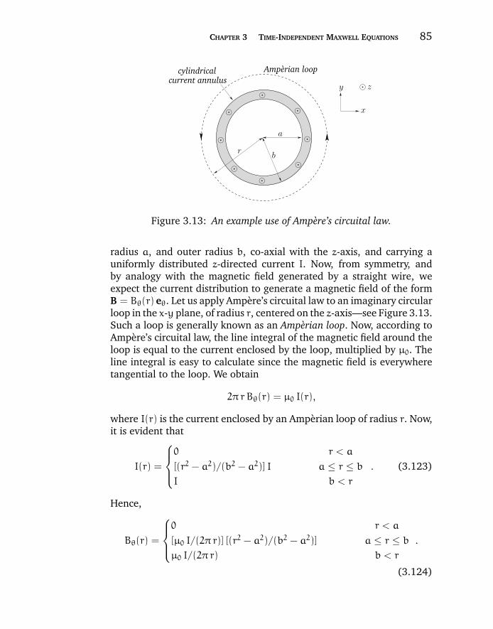
“chapter3” — 2007/12/14 — 12:02 — page 85 — #37
CHAPTER 3 TIME-INDEPENDENT MAXWELL EQUATIONS 85
z
y
a
br
cylindricalcurrent annulus
Amperian loop
x
Figure 3.13: An example use of Ampere’s circuital law.
radius a, and outer radius b, co-axial with the z-axis, and carrying auniformly distributed z-directed current I. Now, from symmetry, andby analogy with the magnetic field generated by a straight wire, weexpect the current distribution to generate a magnetic field of the formB = Bθ(r) eθ. Let us apply Ampere’s circuital law to an imaginary circularloop in the x-y plane, of radius r, centered on the z-axis—see Figure 3.13.Such a loop is generally known as an Amperian loop. Now, according toAmpere’s circuital law, the line integral of the magnetic field around theloop is equal to the current enclosed by the loop, multiplied by µ0. Theline integral is easy to calculate since the magnetic field is everywheretangential to the loop. We obtain
2π rBθ(r) = µ0 I(r),
where I(r) is the current enclosed by an Amperian loop of radius r. Now,it is evident that
I(r) =
0 r < a
[(r2 − a2)/(b2 − a2)] I a ≤ r ≤ b
I b < r
. (3.123)
Hence,
Bθ(r) =
0 r < a
[µ0 I/(2π r)] [(r2 − a2)/(b2 − a2)] a ≤ r ≤ b
µ0 I/(2π r) b < r
.
(3.124)
“chapter3” — 2007/12/14 — 12:02 — page 86 — #38
86 MAXWELL’S EQUATIONS AND THE PRINCIPLES OF ELECTROMAGNETISM
3.11 HELMHOLTZ’S THEOREM
Up to now, we have only studied the electric and magnetic fields gen-erated by stationary charges and steady currents. We have found thatthese fields are describable in terms of four field equations: i.e.,
∇ · E =ρ
ε0, (3.125)
∇ × E = 0 (3.126)
for electric fields, and
∇ · B = 0, (3.127)
∇ × B = µ0 j (3.128)
for magnetic fields. There are no other field equations. This stronglysuggests that if we know the divergence and the curl of a vector fieldthen we know everything there is to know about the field. In fact, thisis the case. There is a mathematical theorem which sums this up. It iscalled Helmholtz’s theorem, after the German polymath Hermann LudwigFerdinand von Helmholtz.
Let us start with scalar fields. Field equations are a type of differentialequation: i.e., they deal with the infinitesimal differences in quantitiesbetween neighbouring points. So what kind of differential equation com-pletely specifies a scalar field? This is easy. Suppose that we have a scalarfield φ(r) and a field equation which tells us the gradient of this field atall points: something like
∇φ = A, (3.129)
where A(r) is a vector field. Note that we need ∇ × A = 0 for self-consistency, since the curl of a gradient is automatically zero. The aboveequation completely specifies φ(r) once we are given the value of thefield at a single point, P (say). Thus,
φ(Q) = φ(P) +
∫QP
∇φ · dl = φ(P) +
∫QP
A · dl, (3.130)
where Q is a general point. The fact that ∇ × A = 0 means that A isa conservative field, which guarantees that the above equation gives aunique value for φ at a general point in space.
Suppose that we have a vector field F(r). How many differentialequations do we need to completely specify this field? Hopefully, we onlyneed two: one giving the divergence of the field, and one giving its curl.
“chapter3” — 2007/12/14 — 12:02 — page 87 — #39
CHAPTER 3 TIME-INDEPENDENT MAXWELL EQUATIONS 87
Let us test this hypothesis. Suppose that we have two field equations:
∇ · F = D, (3.131)
∇ × F = C, (3.132)
whereD(r) is a scalar field and C(r) is a vector field. For self-consistency,we need
∇ · C = 0, (3.133)
since the divergence of a curl is automatically zero. So, do these two fieldequations, plus some suitable boundary conditions, completely specifyF? Suppose that we write
F = −∇U+ ∇ × W. (3.134)
In other words, we are saying that a general vector field F is the sum of aconservative field, ∇U, and a solenoidal field, ∇ × W. This sounds plau-sible, but it remains to be proved. Let us start by taking the divergenceof the above equation, and making use of Equation (3.131). We get
∇2U = −D. (3.135)
Note that the vector field W does not figure in this equation, becausethe divergence of a curl is automatically zero. Let us now take the curlof Equation (3.134):
∇ × F = ∇ × ∇ × W = ∇(∇ · W) − ∇2W = −∇2W. (3.136)
Here, we assume that the divergence of W is zero. This is another thingwhich remains to be proved. Note that the scalar field U does not figurein this equation, because the curl of a divergence is automatically zero.Using Equation (3.132), we get
∇2Wx = −Cx, (3.137)
∇2Wy = −Cy, (3.138)
∇2Wz = −Cz, (3.139)
So, we have transformed our problem into four differential equations,Equation (3.135) and Equations (3.137)–(3.139), which we need tosolve. Let us look at these equations. We immediately notice that theyall have exactly the same form. In fact, they are all versions of Poisson’s
“chapter3” — 2007/12/14 — 12:02 — page 88 — #40
88 MAXWELL’S EQUATIONS AND THE PRINCIPLES OF ELECTROMAGNETISM
equation. We can now make use of a principle made famous by RichardP. Feynman: “the same equations have the same solutions.” Recall thatearlier on we came across the following equation:
∇2φ = −ρ
ε0, (3.140)
where φ is the electrostatic potential and ρ is the charge density. Weproved that the solution to this equation, with the boundary conditionthat φ goes to zero at infinity, is
φ(r) =1
4πε0
∫ρ(r ′)
|r − r ′|d3r ′. (3.141)
Well, if the same equations have the same solutions, and Equa-tion (3.141) is the solution to Equation (3.140), then we can immediatelywrite down the solutions to Equation (3.135) and Equations (3.137)–(3.139). We get
U(r) =1
4π
∫D(r ′)|r − r ′|
d3r ′, (3.142)
and
Wx(r) =1
4π
∫Cx(r ′)|r − r ′|
d3r ′, (3.143)
Wy(r) =1
4π
∫Cy(r ′)|r − r ′|
d3r ′, (3.144)
Wz(r) =1
4π
∫Cz(r ′)|r − r ′|
d3r ′. (3.145)
The last three equations can be combined to form a single vectorequation:
W(r) =1
4π
∫C(r ′)|r − r ′|
d3r ′. (3.146)
We assumed earlier that ∇ · W = 0. Let us check to see if this is true.Note that
∂
∂x
(1
|r − r ′|
)= −
x− x ′
|r − r ′|3=x ′ − x
|r − r ′|3= −
∂
∂x ′
(1
|r − r ′|
), (3.147)
which implies that
∇(
1
|r − r ′|
)= −∇ ′
(1
|r − r ′|
), (3.148)
“chapter3” — 2007/12/14 — 12:02 — page 89 — #41
CHAPTER 3 TIME-INDEPENDENT MAXWELL EQUATIONS 89
where ∇ ′ is the operator (∂/∂x ′, ∂/∂y ′, ∂/∂z ′). Taking the divergence ofEquation (3.146), and making use of the above relation, we obtain
∇ · W =1
4π
∫C(r ′) · ∇
(1
|r − r ′|
)d3r ′
= −1
4π
∫C(r ′) · ∇ ′
(1
|r − r ′|
)d3r ′. (3.149)
Now ∫∞
−∞
g∂f
∂xdx = [g f]∞−∞
−
∫∞
−∞
f∂g
∂xdx. (3.150)
However, if g f → 0 as x → ±∞ then we can neglect the first term on theright-hand side of the above equation and write∫
∞
−∞
g∂f
∂xdx = −
∫∞
−∞
f∂g
∂xdx. (3.151)
A simple generalization of this result yields∫g · ∇f d3r = −
∫f∇ · g d3r, (3.152)
provided that gx f → 0 as |r| → ∞, etc. Thus, we can deduce that
∇ · W =1
4π
∫ ∇ ′ ·C(r ′)|r − r ′|
d3r ′ (3.153)
from Equation (3.149), provided |C(r)|, is bounded as |r| → ∞. However,we have already shown that ∇ · C = 0 from self-consistency arguments,so the above equation implies that ∇ · W = 0, which is the desired result.
We have constructed a vector field F(r) which satisfies Equa-tions (3.131) and (3.132) and behaves sensibly at infinity: i.e., |F| → 0
as |r| → ∞. But, is our solution the only possible solution of Equa-tions (3.131) and (3.132) with sensible boundary conditions at infinity?Another way of posing this question is to ask whether there are anysolutions of
∇2U = 0, ∇2Wi = 0, (3.154)
where i denotes x, y, or z, which are bounded at infinity. If there arethen we are in trouble, because we can take our solution and add toit an arbitrary amount of a vector field with zero divergence and zerocurl, and thereby obtain another solution which also satisfies physicalboundary conditions. This would imply that our solution is not unique.
“chapter3” — 2007/12/14 — 12:02 — page 90 — #42
90 MAXWELL’S EQUATIONS AND THE PRINCIPLES OF ELECTROMAGNETISM
In other words, it is not possible to unambiguously reconstruct a vectorfield given its divergence, its curl, and physical boundary conditions.Fortunately, the equation
∇2φ = 0, (3.155)
which is called Laplace’s equation, has a very interesting property: itssolutions are unique. That is, if we can find a solution to Laplace’s equa-tion which satisfies the boundary conditions then we are guaranteed thatthis is the only solution. We shall prove this later on in Section 5.8. Well,let us invent some solutions to Equations (3.154) which are bounded atinfinity. How about
U = Wi = 0 ? (3.156)
These solutions certainly satisfy Laplace’s equation, and are well-behaved at infinity. Because the solutions to Laplace’s equations areunique, we know that Equations (3.156) are the only solutions to Equa-tions (3.154). This means that there is no vector field which satisfiesphysical boundary equations at infinity and has zero divergence and zerocurl. In other words, our solution to Equations (3.131) and (3.132) isthe only solution. Thus, we have unambiguously reconstructed the vec-tor field F given its divergence, its curl, and sensible boundary conditionsat infinity. This is Helmholtz’s theorem.
We have just demonstrated a number of very useful, and also veryimportant, points. First, according to Equation (3.134), a general vectorfield can be written as the sum of a conservative field and a solenoidalfield. Thus, we ought to be able to write electric and magnetic fieldsin this form. Second, a general vector field which is zero at infinity iscompletely specified once its divergence and its curl are given. Thus, wecan guess that the laws of electromagnetism can be written as four fieldequations,
∇ · E = something, (3.157)
∇ × E = something, (3.158)
∇ · B = something, (3.159)
∇ × B = something, (3.160)
without knowing the first thing about electromagnetism (other than thefact that it deals with two vector fields). Of course, Equations (3.125)–(3.128) are of exactly this form. We also know that there are only fourfield equations, since the above equations are sufficient to completely
“chapter3” — 2007/12/14 — 12:02 — page 91 — #43
CHAPTER 3 TIME-INDEPENDENT MAXWELL EQUATIONS 91
reconstruct both E and B. Furthermore, we know that we can solve thefield equations without even knowing what the right-hand sides looklike. After all, we solved Equations (3.131)–(3.132) for completely gen-eral right-hand sides. [Actually, the right-hand sides have to go to zeroat infinity, otherwise integrals like Equation (3.142) blow up.] We alsoknow that any solutions we find are unique. In other words, there isonly one possible steady electric and magnetic field which can be gener-ated by a given set of stationary charges and steady currents. The thirdthing which we proved was that if the right-hand sides of the above fieldequations are all zero then the only physical solution is E(r) = B(r) = 0.This implies that steady electric and magnetic fields cannot generatethemselves. Instead, they have to be generated by stationary chargesand steady currents. So, if we come across a steady electric field thenwe know that if we trace the field-lines back we shall eventually find acharge. Likewise, a steady magnetic field implies that there is a steadycurrent flowing somewhere. All of these results follow from vector fieldtheory (i.e., from the mathematical properties of vector fields in three-dimensional space), prior to any investigation of electromagnetism.
3.12 THE MAGNETIC VECTOR POTENTIAL
Electric fields generated by stationary charges obey
∇ × E = 0. (3.161)
This immediately allows us to write
E = −∇φ, (3.162)
since the curl of a gradient is automatically zero. In fact, whenever wecome across an irrotational vector field in Physics we can always writeit as the gradient of some scalar field. This is clearly a useful thing todo, since it enables us to replace a vector field by a much simpler scalarfield. The quantity φ in the above equation is known as the electric scalarpotential.
Magnetic fields generated by steady currents (and unsteady currents,for that matter) satisfy
∇ · B = 0. (3.163)
This immediately allows us to write
B = ∇ × A, (3.164)
“chapter3” — 2007/12/14 — 12:02 — page 92 — #44
92 MAXWELL’S EQUATIONS AND THE PRINCIPLES OF ELECTROMAGNETISM
since the divergence of a curl is automatically zero. In fact, wheneverwe come across a solenoidal vector field in Physics we can always writeit as the curl of some other vector field. This is not an obviously usefulthing to do, however, since it only allows us to replace one vector fieldby another. Nevertheless, Equation (3.164) is one of the most usefulequations we shall come across in this book. The quantity A is known asthe magnetic vector potential.
We know from Helmholtz’s theorem that a vector field is fully spec-ified by its divergence and its curl. The curl of the vector potential givesus the magnetic field via Equation (3.164). However, the divergence ofA has no physical significance. In fact, we are completely free to choose∇ · A to be whatever we like. Note that, according to Equation (3.164),the magnetic field is invariant under the transformation
A → A − ∇ψ. (3.165)
In other words, the vector potential is undetermined to the gradientof a scalar field. This is just another way of saying that we are free tochoose ∇ · A. Recall that the electric scalar potential is undetermined toan arbitrary additive constant, since the transformation
φ → φ+ c (3.166)
leaves the electric field invariant in Equation (3.162). The transforma-tions (3.165) and (3.166) are examples of what mathematicians callgauge transformations. The choice of a particular function ψ or a partic-ular constant c is referred to as a choice of the gauge. We are free to fixthe gauge to be whatever we like. The most sensible choice is the onewhich makes our equations as simple as possible. The usual gauge forthe scalar potential φ is such that φ → 0 at infinity. The usual gauge forA (in steady-state situations) is such that
∇ · A = 0. (3.167)
This particular choice is known as the Coulomb gauge.It is obvious that we can always add a constant to φ so as to make
it zero at infinity. But it is not at all obvious that we can always performa gauge transformation such as to make ∇ · A zero. Suppose that wehave found some vector field A(r) whose curl gives the magnetic fieldbut whose divergence in non-zero. Let
∇ · A = v(r). (3.168)
So, can we find a scalar field ψ such that after we perform the gaugetransformation (3.165) we are left with ∇ · A = 0? Taking the divergence
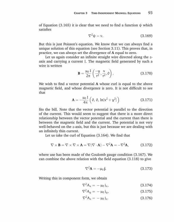
“chapter3” — 2007/12/14 — 12:02 — page 93 — #45
CHAPTER 3 TIME-INDEPENDENT MAXWELL EQUATIONS 93
of Equation (3.165) it is clear that we need to find a function ψ whichsatisfies
∇2ψ = v. (3.169)
But this is just Poisson’s equation. We know that we can always find aunique solution of this equation (see Section 3.11). This proves that, inpractice, we can always set the divergence of A equal to zero.
Let us again consider an infinite straight wire directed along the z-axis and carrying a current I. The magnetic field generated by such awire is written
B =µ0 I
2π
(−y
r2,x
r2, 0
). (3.170)
We wish to find a vector potential A whose curl is equal to the abovemagnetic field, and whose divergence is zero. It is not difficult to seethat
A = −µ0 I
4π
(0, 0, ln[x2 + y2]
)(3.171)
fits the bill. Note that the vector potential is parallel to the directionof the current. This would seem to suggest that there is a more directrelationship between the vector potential and the current than there isbetween the magnetic field and the current. The potential is not verywell-behaved on the z-axis, but this is just because we are dealing withan infinitely thin current.
Let us take the curl of Equation (3.164). We find that
∇ × B = ∇ × ∇ × A = ∇(∇ · A) − ∇2A = −∇2A, (3.172)
where use has been made of the Coulomb gauge condition (3.167). Wecan combine the above relation with the field equation (3.118) to give
∇2A = −µ0 j. (3.173)
Writing this in component form, we obtain
∇2Ax = − µ0 jx, (3.174)
∇2Ay = − µ0 jy, (3.175)
∇2Az = − µ0 jz. (3.176)
“chapter3” — 2007/12/14 — 12:02 — page 94 — #46
94 MAXWELL’S EQUATIONS AND THE PRINCIPLES OF ELECTROMAGNETISM
But, this is just Poisson’s equation three times over. We can immediatelywrite the unique solutions to the above equations:
Ax(r) =µ0
4π
∫jx(r ′)|r − r ′|
d3r ′, (3.177)
Ay(r) =µ0
4π
∫jy(r ′)|r − r ′|
d3r ′, (3.178)
Az(r) =µ0
4π
∫jz(r ′)|r − r ′|
d3r ′. (3.179)
These solutions can be recombined to form a single vector solution
A(r) =µ0
4π
∫j(r ′)
|r − r ′|d3r ′. (3.180)
Of course, we have seen a equation like this before:
φ(r) =1
4πε0
∫ρ(r ′)
|r − r ′|d3r ′. (3.181)
Equations (3.180) and (3.181) are the unique solutions (given the arbi-trary choice of gauge) to the field equations (3.125)–(3.128): theyspecify the magnetic vector and electric scalar potentials generated bya set of stationary charges, of charge density ρ(r), and a set of steadycurrents, of current density j(r). Incidentally, we can prove that Equa-tion (3.180) satisfies the gauge condition ∇ · A = 0 by repeating theanalysis of Equations (3.146)–(3.153) (with W → A and C → µ0 j), andusing the fact that ∇ · j = 0 for steady currents.
As an example, let us find the vector potential associated with themagnetic field distribution (3.124). By symmetry, and by analogy withthe vector potential generated by a straight wire, we expect that A =Az(r) ez. Note that this form for A satisfies the Coulomb gauge. Hence,using ∇ × A = B, we get
∂Az
∂r= −Bθ(r). (3.182)
The boundary conditions are that Az be continuous at r = a and r =b, since a discontinuous Az would generate an infinite magnetic field,which is unphysical. Thus, we obtain
Az(r) =
(µ0 I/2π) [1/2− a2 ln(b/a)/(b2 − a2)] r < a
(µ0 I/2π) ([b2/2− r2/2− a2 ln(b/r)]/[b2 − a2]) a ≤ r ≤ b
−(µ0 I/2π) ln(r/b) b < r
.
(3.183)
“chapter3” — 2007/12/14 — 12:02 — page 95 — #47
CHAPTER 3 TIME-INDEPENDENT MAXWELL EQUATIONS 95
3.13 THE BIOT-SAVART LAW
According to Equation (3.162), we can obtain an expression for the elec-tric field generated by stationary charges by taking minus the gradientof Equation (3.181). This yields
E(r) =1
4πε0
∫ρ(r ′)
r − r ′
|r − r ′|3d3r ′, (3.184)
which we recognize as Coulomb’s law written for a continuous chargedistribution. According to Equation (3.164), we can obtain an equivalentexpression for the magnetic field generated by steady currents by takingthe curl of Equation (3.180). This gives
B(r) =µ0
4π
∫j(r ′) × (r − r ′)
|r − r ′|3d3r ′, (3.185)
where use has been made of the vector identity ∇ × (φA) = φ∇ ×A + ∇φ× A. Equation (3.185) is known as the Biot-Savart law afterthe French physicists Jean Baptiste Biot and Felix Savart: it completelyspecifies the magnetic field generated by a steady (but otherwise quitegeneral) distributed current.
Let us reduce our distributed current to an idealized zero-thicknesswire. We can do this by writing
j(r)d3r = I(r)dl, (3.186)
where I is the vector current (i.e., its direction and magnitude specify thedirection and magnitude of the current) and dl is an element of lengthalong the wire. Equations (3.185) and (3.186) can be combined to give
B(r) =µ0
4π
∫I(r ′) × (r − r ′)
|r − r ′|3dl, (3.187)
which is the form in which the Biot-Savart law is most usually written.This law is to magnetostatics (i.e., the study of magnetic fields generatedby steady currents) what Coulomb’s law is to electrostatics (i.e., the studyof electric fields generated by stationary charges). Furthermore, it canbe experimentally verified given a set of currents, a compass, a testwire, and a great deal of skill and patience. This justifies our earlierassumption that the field equations (3.121) and (3.122) are valid forgeneral current distributions (recall that we derived them by studyingthe fields generated by infinite straight wires). Note that both Coulomb’slaw and the Biot-Savart law are gauge independent: i.e., they do notdepend on the particular choice of gauge.
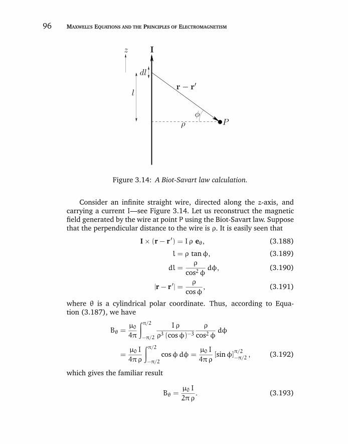
“chapter3” — 2007/12/14 — 12:02 — page 96 — #48
96 MAXWELL’S EQUATIONS AND THE PRINCIPLES OF ELECTROMAGNETISM
z
dl
I
lr − r′
φρ P
Figure 3.14: A Biot-Savart law calculation.
Consider an infinite straight wire, directed along the z-axis, andcarrying a current I—see Figure 3.14. Let us reconstruct the magneticfield generated by the wire at point P using the Biot-Savart law. Supposethat the perpendicular distance to the wire is ρ. It is easily seen that
I × (r − r ′) = I ρ eθ, (3.188)
l = ρ tanφ, (3.189)
dl =ρ
cos2 φdφ, (3.190)
|r − r ′| =ρ
cosφ, (3.191)
where θ is a cylindrical polar coordinate. Thus, according to Equa-tion (3.187), we have
Bθ =µ0
4π
∫π/2−π/2
I ρ
ρ3 (cosφ)−3
ρ
cos2 φdφ
=µ0 I
4π ρ
∫π/2−π/2
cosφdφ =µ0 I
4π ρ[sinφ]
π/2
−π/2, (3.192)
which gives the familiar result
Bθ =µ0 I
2π ρ. (3.193)
“chapter3” — 2007/12/14 — 12:02 — page 97 — #49
CHAPTER 3 TIME-INDEPENDENT MAXWELL EQUATIONS 97
So, we have come full circle in our investigation of magnetic fields. Notethat the simple result (3.193) can only be obtained from the Biot-Savartlaw after some non-trivial algebra. Examination of more complicatedcurrent distributions using this law invariably leads to lengthy, involved,and extremely unpleasant calculations.
3.14 ELECTROSTATICS AND MAGNETOSTATICS
We have now completed our theoretical investigation of electrostaticsand magnetostatics. Our next task is to incorporate time variation intoour analysis. However, before we start this, let us briefly review ourprogress so far. We have found that the electric fields generated by sta-tionary charges, and the magnetic fields generated by steady currents,are describable in terms of four field equations:
∇ · E =ρ
ε0, (3.194)
∇ × E = 0, (3.195)
∇ · B = 0, (3.196)
∇ × B = µ0 j. (3.197)
The boundary conditions are that the fields are zero at infinity, assumingthat the generating charges and currents are localized to some region inspace. According to Helmholtz’s theorem, the above field equations, plusthe boundary conditions, are sufficient to uniquely specify the electricand magnetic fields. The physical significance of this is that divergenceand curl are the only rotationally invariant first-order differential proper-ties of a general vector field: i.e., the only quantities which do not changetheir physical characteristics when the coordinate axes are rotated. SincePhysics does not depend on the orientation of the coordinate axes (whichis, after all, quite arbitrary), it follows that divergence and curl are theonly quantities which can appear in first-order differential field equationswhich claim to describe physical phenomena.
The field equations can be integrated to give:
∮S
E · dS =1
ε0
∫V
ρdV, (3.198)
∮C
E · dl = 0, (3.199)
“chapter3” — 2007/12/14 — 12:02 — page 98 — #50
98 MAXWELL’S EQUATIONS AND THE PRINCIPLES OF ELECTROMAGNETISM
∮S
B · dS = 0, (3.200)
∮C
B · dl = µ0
∫S ′
j · dS. (3.201)
Here, S is a closed surface enclosing a volume V. Also, C is a closedloop, and S ′ is some surface attached to this loop. The field equations(3.194)–(3.197) can be deduced from Equations (3.198)–(3.201) usingGauss’ theorem and Stokes’ theorem. Equation (3.198) is called Gauss’law, and says that the flux of the electric field out of a closed surfaceis proportional to the enclosed electric charge. Equation (3.200) has noparticular name, and says that there is no such things as a magneticmonopole. Equation (3.201) is called Ampere’s circuital law, and saysthat the line integral of the magnetic field around any closed loop isproportional to the flux of the current density through the loop.
The field equation (3.195) is automatically satisfied if we write
E = −∇φ. (3.202)
Likewise, the field equation (3.196) is automatically satisfied if we write
B = ∇ × A. (3.203)
Here, φ is the electric scalar potential, and A is the magnetic vectorpotential. The electric field is clearly unchanged if we add a constant tothe scalar potential:
E → E as φ → φ+ c. (3.204)
The magnetic field is similarly unchanged if we subtract the gradient ofa scalar field from the vector potential:
B → B as A → A − ∇ψ. (3.205)
The above transformations, which leave the E and B fields invariant,are called gauge transformations. We are free to choose c and ψ to bewhatever we like: i.e., we are free to choose the gauge. The most sensiblegauge is the one which makes our equations as simple and symmetric aspossible. This corresponds to the choice
φ(r) → 0 as |r| → ∞, (3.206)
and
∇ · A = 0. (3.207)
The latter convention is known as the Coulomb gauge.
“chapter3” — 2007/12/14 — 12:02 — page 99 — #51
CHAPTER 3 TIME-INDEPENDENT MAXWELL EQUATIONS 99
Taking the divergence of Equation (3.202) and the curl of Equa-tion (3.203), and making use of the Coulomb gauge, we find that the fourfield equations (3.194)–(3.197) can be reduced to Poisson’s equationwritten four times over:
∇2φ = −ρ
ε0, (3.208)
∇2A = − µ0 j. (3.209)
Poisson’s equation is just about the simplest rotationally invariantsecond-order partial differential equation it is possible to write. Note that∇2 is clearly rotationally invariant, since it is the divergence of a gradi-ent, and both divergence and gradient are rotationally invariant. We canalways construct the solution to Poisson’s equation, given the boundaryconditions. Furthermore, we have a uniqueness theorem which tells usthat our solution is the only possible solution. Physically, this meansthat there is only one electric and magnetic field which is consistentwith a given set of stationary charges and steady currents. This soundslike an obvious, almost trivial, statement. But there are many areas ofPhysics (for instance, Fluid Mechanics and Plasma Physics) where wealso believe, for physical reasons, that for a given set of boundary condi-tions the solution should be unique. The difficulty is that in most caseswhen we reduce a given problem to a partial differential equation weend up with something far nastier than Poisson’s equation. In general,we cannot solve this equation. In fact, we usually cannot even provethat it possess a solution for general boundary conditions, let alone thatthe solution is unique. So, we are very fortunate indeed that in Elec-trostatics and Magnetostatics a general problem always boils down tosolving a tractable partial differential equation. When physicists makestatements to the effect that “Electromagnetism is the best understoodtheory in Physics,” which they often do, what they are really saying isthat the partial differential equations which crop up in this theory aresoluble and have unique solutions.
Poisson’s equation
∇2u = v (3.210)
is linear, which means that its solutions are superposable. We can exploitthis fact to construct a general solution to this equation. Suppose thatwe can find the solution to
∇2G(r, r ′) = δ(r − r ′) (3.211)
“chapter3” — 2007/12/14 — 12:02 — page 100 — #52
100 MAXWELL’S EQUATIONS AND THE PRINCIPLES OF ELECTROMAGNETISM
which satisfies the boundary conditions. This is the solution driven bya unit amplitude point source located at position vector r ′. Since anygeneral source can be built up out of a weighted sum of point sources,it follows that a general solution to Poisson’s equation can be builtup out of a similarly weighted superposition of point source solutions.Mathematically, we can write
u(r) =
∫G(r, r ′) v(r ′)d3r ′. (3.212)
The function G(r, r ′) is called the Green’s function. The Green’s functionfor Poisson’s equation is
G(r, r ′) = −1
4π
1
|r − r ′|. (3.213)
Note that this Green’s function is proportional to the scalar potential of apoint charge located at r ′: this is hardly surprising, given the definitionof a Green’s function.
According to Equations (3.208), (3.209), (3.210), (3.212), and(3.213), the scalar and vector potentials generated by a set of stationarycharges and steady currents take the form
φ(r) =1
4πε0
∫ρ(r ′)
|r − r ′|d3r ′, (3.214)
A(r) =µ0
4π
∫j(r ′)
|r − r ′|d3r ′. (3.215)
Making use of Equations (3.202), (3.203), (3.214), and (3.215), weobtain Coulomb’s law,
E(r) =1
4πε0
∫ρ(r ′)
r − r ′
|r − r ′|3d3r ′, (3.216)
and the Biot-Savart law,
B(r) =µ0
4π
∫j(r ′) × (r − r ′)
|r − r ′|3d3r ′. (3.217)
Of course, both of these laws are examples of action-at-a-distance laws(in that the electric and magnetic fields at a given point respond instanta-neously to changes in the charge and current densities at distant points),and, therefore, violate the Special Theory of Relativity. However, this is
“chapter3” — 2007/12/14 — 12:02 — page 101 — #53
CHAPTER 3 TIME-INDEPENDENT MAXWELL EQUATIONS 101
not a problem as long as we restrict ourselves to fields generated bytime-independent charge and current distributions.
The next question is by how much is this scheme which we havejust worked out going to be disrupted when we take time variation intoaccount. The answer, somewhat surprisingly, is by very little indeed. So,in Equations (3.194)–(3.217) we can already discern the basic outlineof Classical Electromagnetism. Let us continue our investigation.
3.15 EXERCISES
3.1. A charge Q is uniformly distributed in a sphere of radius a centered on the
origin. Use symmetry and Gauss’ law to find the electric field generated inside
and outside the sphere. What is the corresponding electric potential inside and
outside the sphere?
3.2. A charge per unit lengthQ is uniformly distributed in an infinitely long cylinder
of radius a whose axis corresponds to the z-axis. Use symmetry and Gauss’ law
to find the electric field generated inside and outside the cylinder. What is the
corresponding electric potential inside and outside the cylinder.
3.3. Find the electric charge distribution which generates the Yukawa potential
φ(r) =q
4πε0
e−r/a
r,
where r is a spherical polar coordinate, and a a positive constant. Why must the
total charge in the distribution be zero?
3.4. An electric dipole consists of two equal and opposite charges, q and −q, sep-
arated by a small distance d. The strength and orientation of the dipole is
measured by its vector moment p, which is of magnitude qd, and points in the
direction of the displacement of the positive charge from the negative. Use the
principle of superposition to demonstrate that the electric potential generated
by an electric dipole of moment p situated at the origin is
φ(r) =p · r4πε0 r3
.
Show that the corresponding electric field distribution is
E(r) =3 (p · r) r − r2 p
4πε0 r5.
3.5. An electric dipole of fixed moment p is situated at position r in a non-uniform
external electric field E(r). Demonstrate that the net force on the dipole can be
“chapter3” — 2007/12/14 — 12:02 — page 102 — #54
102 MAXWELL’S EQUATIONS AND THE PRINCIPLES OF ELECTROMAGNETISM
written f = −∇W, where
W = −p · E.
Hence, show that the potential energy of an electric dipole of moment p1 in the
electric field generated by a second dipole of moment p2 is
W =r2 (p1 · p2) − 3 (p1 · r) (p2 · r)
4πε0 r5,
where r is the displacement of one dipole from another.
3.6. Show that the torque on an electric dipole of moment p in a uniform external
electric field E is
τ = p × E.
Hence, deduce that the potential energy of the dipole is
W = −p · E.
3.7. A charge distribution ρ(r) is localized in the vicinity of the origin in a region of
radius a. Consider the electric potential generated at position r, where |r| a.
Demonstrate via a suitable expansion in a/r that
φ(r) =Q
4πε0 r+
p · r4πε0 r3
+ · · · ,
where Q =∫ρ(r)d3r is the total charge contained in the distribution, and p =
∫ρ(r) r d3r its electric dipole moment.
3.8. Consider a scalar potential field φ(r) generated by a set of stationary charges.
Demonstrate that the mean potential over any spherical surface which does not
contain a charge is equal to the potential at the center. Hence, deduce that there
can be no maxima or minima of the scalar potential in a charge-free region. Hint:
The solution to this problem is more intuitive than mathematical, and depends
on the fact that the potential generated outside a uniform spherical charge shell
is the same as that generated when all of the charge is collected at its center.
3.9. Demonstrate that the Green’s function for Poisson’s equation in two dimensions
(i.e., ∂/∂z ≡ 0) is
G(r, r ′) = −ln |r − r ′|2π
,
where r = (x, y), etc. Hence, deduce that the scalar potential field generated by
the two-dimensional charge distribution ρ(r) is
φ(r) = −1
2πε0
∫ρ(r ′) ln |r − r ′
|d3r ′.
3.10. A particle of mass m and charge q starts at rest from the origin at t = 0 in a
uniform electric field E directed along the y-axis, and a uniform magnetic field
“chapter3” — 2007/12/14 — 12:02 — page 103 — #55
CHAPTER 3 TIME-INDEPENDENT MAXWELL EQUATIONS 103
B directed along the z-axis. Find the particle’s subsequent motion in the x-y
plane. Sketch the particle’s trajectory.
3.11. In a parallel-plate magnetron the cathode and the anode are flat parallel plates,
and a uniform magnetic field B is applied in a direction parallel to the plates.
Electrons are emitted from the cathode with essentially zero velocity. If the
separation between the anode and cathode is d, and if the anode is held at a
constant positive potential V with respect to the cathode, show that no current
will flow between the plates when
V ≤ eB2 d2
2me
.
Here, e is the magnitude of the electron charge, and me the electron mass.
3.12. An infinite, straight, circular cross-section wire of radius a runs along the z-
axis and carries a uniformly distributed z-directed current I. Use symmetry and
Ampere’s circuital law to find the magnetic field distribution inside and out-
side the wire. What is the corresponding magnetic vector potential inside and
outside the wire? Use the Coulomb gauge.
3.13. An infinite cylindrical current annulus of inner radius a, outer radius b, and axis
running along the z-axis carries a uniformly distributed current per unit length
I in the θ direction: i.e., j ∝ eθ. Use symmetry and Ampere’s circuital law to
find the magnetic field distribution inside and outside the annulus. What is the
corresponding magnetic vector potential inside and outside the annulus? Use
the Coulomb gauge.
3.14. A thick slab extends from z = −a to z = a, and is infinite in the x-y plane.
The slab carries a uniform current density j = J ex. Find the magnetic field
and magnetic vector potential inside and outside the slab. Use the Coulomb
gauge.
3.15. Show that the magnetic vector potential due to two long, straight, z-directed
wires, the first carrying a current I, and the second a current −I, is
A =µ0 I
2πln
(r1
r2
)ez,
where r1 and r2 are the perpendicular distances to the two wires.
3.16. Use the Biot-Savart law to:
(a) Find the magnetic field at the center of a circular loop of radius r carrying
a current I.
(b) Find the magnetic field at the center of a square loop carrying a current
I. Let r be the perpendicular distance from the center to one of the sides
of the loop.
“chapter3” — 2007/12/14 — 12:02 — page 104 — #56
104 MAXWELL’S EQUATIONS AND THE PRINCIPLES OF ELECTROMAGNETISM
(c) Find the magnetic field at the center of a regular n-sided polygon car-
rying a current I. Let r be the perpendicular distance from the center
to one of the sides of the loop. Check that your answer reduces to the
answer from part (a) in the limit n → ∞.
3.17. Use the Biot-Savart law to show that the magnetic field generated along the axis
of a circular current loop of radius a lying in the x-y plane and centered on the
origin is
Bz =µ0 I
2
a2
(a2 + z2)3/2.
Here, I is the current circulating counterclockwise (looking down the z-axis)
around the loop. Demonstrate that∫
∞
−∞
Bz(z)dz = µ0 I.
Derive this result from Ampere’s circuital law.
3.18. A Helmholtz coil consists of two identical, single turn, circular coils, of radius
a, carrying the same current, I, in the same sense, which are coaxial with one
another, and are separated by a distance d. Show that the variation of the mag-
netic field-strength in the vicinity of the axial midpoint is minimized when d = a.
Demonstrate that, in this optimal case, the magnetic field-strength at the axial
midpoint is
B =8 µ0 I
5√5 a.
3.19. A force-free magnetic field is such that j × B = 0. Demonstrate that such a field
satisfies
∇2B = −α2 B,
where α is some constant. Find the force-free field with the lowest value of α
(excludingα = 0) in a cubic volume of dimensiona bounded by superconducting
walls (in which B = 0).
3.20. Consider a small circular current loop of radius a lying in the x-y plane and
centered on the origin. Such a loop constitutes a magnetic dipole of moment
m, where m = πa2 I, and I is the circulating current. The direction of m is
conventionally taken to be normal to the plane of the loop, in the sense given
by the right-hand grip rule. Demonstrate that the magnetic vector potential
generated at position r, where |r| a, is
A(r) =µ0
4π
m × rr3
.
“chapter3” — 2007/12/14 — 12:02 — page 105 — #57
CHAPTER 3 TIME-INDEPENDENT MAXWELL EQUATIONS 105
Show that the corresponding magnetic field is
B(r) =µ0
4π
(3 (r · m) r − r2 m
r5
).
3.21. Demonstrate that the torque on a magnetic dipole of moment m placed in a
uniform external magnetic field B is
τ = m × B.
Hence, deduce that the potential energy of the magnetic dipole is
W = −m · B.
3.22. Consider two magnetic dipoles, m1 and m2. Suppose that m1 is fixed, whereas
m2 can rotate freely in any direction. Demonstrate that the equilibrium
configuration of the second dipole is such that
tan θ1 = −2 tan θ2,
where θ1 and θ2 are the angles subtended by m1 and m2, respectively, with the
radius vector joining them.

“chapter3” — 2007/12/14 — 12:02 — page 106 — #58
“chapter4” — 2007/11/29 — 13:54 — page 107 — #1
C h a p t e r 4 TIME-DEPENDENTMAXWELL EQUATIONS
4.1 INTRODUCTION
In this chapter, we shall generalize the time-independent Maxwell equa-tions, derived in the previous chapter, to obtain the full set of time-dependent Maxwell equations.
4.2 FARADAY’S LAW
The history of humankind’s development of Physics can be thought of asthe history of the synthesis of ideas. Physicists keep finding that appar-ently disparate phenomena can be understood as different aspects ofsome more fundamental phenomenon. This process has continued until,today, all physical phenomena can be described in terms of three funda-mental forces: Gravity, the Electroweak Force, and the Strong Force. Oneof the main goals of modern physics is to find some way of combiningthese three forces so that all of physics can be described in terms of asingle unified force.
The first great synthesis of ideas in Physics took place in 1666 whenIssac Newton realised that the force which causes apples to fall down-ward is the same as that which maintains the Planets in elliptical orbitsaround the Sun. The second great synthesis, which we are about to studyin more detail, took place in 1830 when Michael Faraday discovered thatElectricity and Magnetism are two aspects of the same phenomenon, usu-ally referred to as Electromagnetism. The third great synthesis, which weshall discuss presently, took place in 1873 when James Clerk Maxwelldemonstrated that light and electromagnetism are intimately related.The last (but, hopefully, not the final) great synthesis took place in 1967when Steve Weinberg and Abdus Salam showed that the electromagneticforce and the weak nuclear force (i.e., the one which is responsible forβ decays) can be combined to give the electroweak force.
Let us now consider Faraday’s experiments, having put them intheir proper historical context. Prior to 1830, the only known way in
107

“chapter4” — 2007/11/29 — 13:54 — page 108 — #2
108 MAXWELL’S EQUATIONS AND THE PRINCIPLES OF ELECTROMAGNETISM
which to make an electric current flow through a conducting wire wasto connect the ends of the wire to the positive and negative terminalsof a battery. We measure a battery’s ability to push current down awire in terms of its voltage, by which we mean the voltage differencebetween its positive and negative terminals. What does voltage corre-spond to in Physics? Well, volts are the units used to measure electricscalar potential, so when we talk about a 6 V battery, what we arereally saying is that the difference in electric scalar potential betweenits positive and negative terminals is six volts. This insight allows us towrite
V = φ(⊕) − φ() = −
∫
⊕∇φ · dl =
∫
⊕E · dl, (4.1)
where V is the battery voltage, ⊕ denotes the positive terminal, thenegative terminal, and dl is an element of length along the wire. Ofcourse, the above equation is a direct consequence of E = −∇φ. Clearly,a voltage difference between two ends of a wire attached to a batteryimplies the presence of a longitudinal electric field which pushes chargesthrough the wire. This field is directed from the positive terminal ofthe battery to the negative terminal, and is, therefore, such as to forceelectrons (which are negatively charged) to flow through the wire fromthe negative to the positive terminal. As expected, this means that a netpositive current flows from the positive to the negative terminal. Thefact that E is a conservative field ensures that the voltage difference Vis independent of the path of the wire between the terminals. In otherwords, two different wires attached to the same battery develop identicalvoltage differences.
Let us now consider a closed loop of wire (with no battery). Thevoltage around such a loop, which is sometimes called the electromotiveforce or emf, is
V =
∮E · dl = 0. (4.2)
The fact that the right-hand side of the above equation is zero is a directconsequence of the field equation ∇ × E = 0. We conclude that, becauseE is a conservative field, the electromotive force around a closed loop ofwire is automatically zero, and so there is no current flow around sucha loop. This all seems to make sense. However, in 1830 Michael Faradaydiscovered that a changing magnetic field can cause a current to flowaround a closed loop of wire (in the absence of a battery). Well, if current
“chapter4” — 2007/11/29 — 13:54 — page 109 — #3
CHAPTER 4 TIME-DEPENDENT MAXWELL EQUATIONS 109
flows around the loop then there must be an electromotive force. So,
V =
∮E · dl = 0, (4.3)
which immediately implies that E is not a conservative field, and that∇ × E = 0. Clearly, we are going to have to modify some of our ideasregarding electric fields.
Faraday continued his experiments, and found that another way ofgenerating an electromotive force around a loop of wire is to keep themagnetic field constant and move the loop. Eventually, Faraday was ableto formulate a law which accounted for all of his experiments—the emfgenerated around a loop of wire in a magnetic field is proportional tothe rate of change of the flux of the magnetic field through the loop. So,if the loop is denoted C, and S is some surface attached to the loop, thenFaraday’s experiments can be summed up by writing
V =
∮C
E · dl = A∂
∂t
∫S
B · dS, (4.4)
where A is a constant of proportionality. Thus, the changing flux ofthe magnetic field through the loop generates an electric field directedaround the loop. This process is know as magnetic induction.
SI units have been carefully chosen so as to make |A| = 1 in the aboveequation. The only thing we now have to decide is whether A = +1 orA = −1. In other words, we need to decide which way around the loopthe induced emf wants to drive the current. We possess a general princi-ple which allows us to decide questions like this. It is called Le Chatelier’sprinciple. According to Le Chatelier’s principle, every change generatesa reaction which tries to minimize the change. Essentially, this meansthat the Universe is stable to small perturbations. When this principleis applied to the special case of magnetic induction, it is usually calledLenz’s law. According to Lenz’s law, the current induced around a closedloop is always such that the magnetic field it produces tries to counter-act the change in magnetic flux which generates the electromotive force.From Figure 4.1, it is clear that if the magnetic field B is increasing andthe current I circulates clockwise (as seen from above) then it gener-ates a field B ′ which opposes the increase in magnetic flux through theloop, in accordance with Lenz’s law. The direction of the current is oppo-site to the sense of the current loop C, as determined by the right-handgrip rule (assuming that the flux of B through the loop is positive), sothis implies that A = −1 in Equation (4.4). Thus, Faraday’s law takes
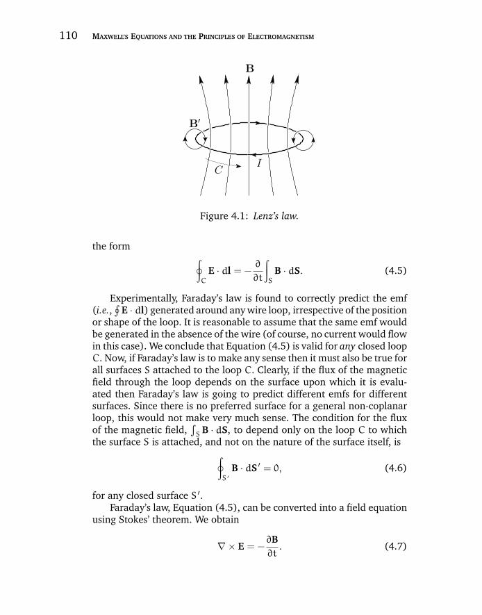
“chapter4” — 2007/11/29 — 13:54 — page 110 — #4
110 MAXWELL’S EQUATIONS AND THE PRINCIPLES OF ELECTROMAGNETISM
B
I
B′
C
Figure 4.1: Lenz’s law.
the form ∮C
E · dl = −∂
∂t
∫S
B · dS. (4.5)
Experimentally, Faraday’s law is found to correctly predict the emf(i.e.,
∮E · dl) generated around any wire loop, irrespective of the position
or shape of the loop. It is reasonable to assume that the same emf wouldbe generated in the absence of the wire (of course, no current would flowin this case). We conclude that Equation (4.5) is valid for any closed loopC. Now, if Faraday’s law is to make any sense then it must also be true forall surfaces S attached to the loop C. Clearly, if the flux of the magneticfield through the loop depends on the surface upon which it is evalu-ated then Faraday’s law is going to predict different emfs for differentsurfaces. Since there is no preferred surface for a general non-coplanarloop, this would not make very much sense. The condition for the fluxof the magnetic field,
∫S
B · dS, to depend only on the loop C to whichthe surface S is attached, and not on the nature of the surface itself, is∮
S ′B · dS ′ = 0, (4.6)
for any closed surface S ′.Faraday’s law, Equation (4.5), can be converted into a field equation
using Stokes’ theorem. We obtain
∇ × E = −∂B∂t. (4.7)
“chapter4” — 2007/11/29 — 13:54 — page 111 — #5
CHAPTER 4 TIME-DEPENDENT MAXWELL EQUATIONS 111
This is the final Maxwell equation. It describes how a changing magneticfield can generate, or induce, an electric field. Gauss’ theorem appliedto Equation (4.6) gives the familiar field equation
∇ · B = 0. (4.8)
This ensures that the magnetic flux through a loop is a well-definedquantity.
The divergence of Equation (4.7) yields
∂∇ · B∂t
= 0. (4.9)
Thus, the field equation (4.7) actually demands that the divergence ofthe magnetic field be constant in time for self-consistency (this meansthat the flux of the magnetic field through a loop need not be a well-defined quantity, as long as its time derivative is well-defined). However,a constant non-solenoidal magnetic field can only be generated by mag-netic monopoles, and magnetic monopoles do not exist (as far as we areaware). Hence, ∇ · B = 0. Note that the absence of magnetic monopolesis an observational fact—it cannot be predicted by any theory. If magneticmonopoles were discovered tomorrow then this would not cause physi-cists any great difficulties, since they know how to generalize Maxwell’sequations to include both magnetic monopoles and currents of mag-netic monopoles. In this generalized formalism, Maxwell’s equations arecompletely symmetric with respect to electric and magnetic fields, and∇ · B = 0. However, an extra term (involving the current of magneticmonopoles) must be added to the right-hand side of Equation (4.7) inorder to make it mathematically self-consistent.
As an example of the use of Faraday’s law, let us calculate the electricfield generated by a decaying magnetic field of the form B = Bz(r, t) ez,where
Bz(r, t) =
B0 exp(−t/τ) r ≤ a
0 r > a. (4.10)
Here, B0 and τ are positive constants. By symmetry, we expect an inducedelectric field of the form E(r, t). We also expect ∇ · E = 0, since thereare no electric charges in the problem. This rules out a radial electricfield. We can also rule out a z-directed electric field, since ∇ × Ez(r) ez =−(∂Ez/∂r) eθ, and we require ∇ × E ∝ B ∝ ez. Hence, the induced elec-tric field must be of the form E(r, t) = Eθ(r, t) eθ. Now, according toFaraday’s law, the line integral of the electric field around some closed
“chapter4” — 2007/11/29 — 13:54 — page 112 — #6
112 MAXWELL’S EQUATIONS AND THE PRINCIPLES OF ELECTROMAGNETISM
loop is equal to minus the rate of change of the magnetic flux throughthe loop. If we choose a loop which is a circle of radius r in the x-y plane,then we have
2π r Eθ(r, t) = −dΦ
dt, (4.11)
where Φ is the magnetic flux (in the +z direction) through a circularloop of radius r. It is evident that
Φ(r, t) =
π r2 B0 exp(−t/τ) r ≤ a
πa2 B0 exp(−t/τ) r > a. (4.12)
Hence,
Eθ(r, t) =
(B0/2 τ) r exp(−t/τ) r ≤ a
(B0/2 τ) (a2/r) exp(−t/τ) r > a. (4.13)
4.3 ELECTRIC SCALAR POTENTIAL?
We now have a problem. We can only write the electric field in terms of ascalar potential (i.e., E = −∇φ) provided that ∇ × E = 0. However, wehave just found that the curl of the electric field is non-zero in the pres-ence of a changing magnetic field. In other words, E is not, in general, aconservative field. Does this mean that we have to abandon the conceptof electric scalar potential? Fortunately, it does not. It is still possible todefine a scalar potential which is physically meaningful.
Let us start from the equation
∇ · B = 0, (4.14)
which is valid for both time-varying and non-time-varying magneticfields. Since the magnetic field is solenoidal, we can write it as the curlof a vector potential:
B = ∇ × A. (4.15)
So, there is no problem with the vector potential in the presence of time-varying fields. Let us substitute Equation (4.15) into the field equation(4.7). We obtain
∇ × E = −∂∇ × A∂t
, (4.16)
“chapter4” — 2007/11/29 — 13:54 — page 113 — #7
CHAPTER 4 TIME-DEPENDENT MAXWELL EQUATIONS 113
which can be written
∇ ×(
E +∂A∂t
)= 0. (4.17)
Now, we know that a curl-free vector field can always be expressed asthe gradient of a scalar potential, so let us write
E +∂A∂t
= −∇φ, (4.18)
or
E = −∇φ−∂A∂t. (4.19)
This equation tells us that the scalar potential φ only describes theconservative electric field generated by electric charges. The electricfield induced by time-varying magnetic fields is non-conservative, and isdescribed by the magnetic vector potential A.
4.4 GAUGE TRANSFORMATIONS
Electric and magnetic fields can be written in terms of scalar and vectorpotentials, as follows:
E = − ∇φ−∂A∂t, (4.20)
B = ∇ × A. (4.21)
However, this prescription is not unique. There are many different poten-tials which can generate the same fields. We have come across thisproblem before. It is called gauge invariance. The most general transfor-mation which leaves the E and B fields unchanged in Equations (4.20)and (4.21) is
φ → φ+∂ψ
∂t, (4.22)
A → A − ∇ψ. (4.23)
This is clearly a generalization of the gauge transformation which wefound earlier for static fields:
φ → φ+ c, (4.24)
A → A − ∇ψ, (4.25)
“chapter4” — 2007/11/29 — 13:54 — page 114 — #8
114 MAXWELL’S EQUATIONS AND THE PRINCIPLES OF ELECTROMAGNETISM
where c is a constant. In fact, if ψ(r, t) → ψ(r) + c t then Equa-tions (4.22) and (4.23) reduce to Equations (4.24) and (4.25).
We are free to choose the gauge so as to make our equations as simpleas possible. As before, the most sensible gauge for the scalar potential isto make it go to zero at infinity:
φ(r, t) → 0 as |r| → ∞. (4.26)
For steady fields, we found that the optimum gauge for the vectorpotential was the so-called Coulomb gauge:
∇ · A = 0. (4.27)
We can still use this gauge for non-steady fields. The argument, whichwe gave earlier (see Section 3.12), that it is always possible to transformaway the divergence of a vector potential remains valid. One of the nicefeatures of the Coulomb gauge is that when we write the electric field,
E = −∇φ−∂A∂t, (4.28)
we find that the part which is generated by charges (i.e., the first term onthe right-hand side) is conservative, and the part induced by magneticfields (i.e., the second term on the right-hand side) is purely solenoidal.Earlier on, we proved mathematically that a general vector field can bewritten as the sum of a conservative field and a solenoidal field (seeSection 3.11). Now we are finding that when we split up the electricfield in this manner the two fields have different physical origins—theconservative part of the field emanates from electric charges, whereasthe solenoidal part is induced by magnetic fields.
Equation (4.28) can be combined with the field equation
∇ · E =ρ
ε0(4.29)
(which remains valid for non-steady fields) to give
−∇2φ−∂∇ · A∂t
=ρ
ε0. (4.30)
With the Coulomb gauge condition, ∇ · A = 0, the above expressionreduces to
∇2φ = −ρ
ε0, (4.31)
which is just Poisson’s equation. Thus, we can immediately write downan expression for the scalar potential generated by non-steady fields. It
“chapter4” — 2007/11/29 — 13:54 — page 115 — #9
CHAPTER 4 TIME-DEPENDENT MAXWELL EQUATIONS 115
is exactly analogous to our previous expression for the scalar potentialgenerated by steady fields: i.e.,
φ(r, t) =1
4πε0
∫ρ(r ′, t)|r − r ′|
d3r ′. (4.32)
However, this apparently simple result is extremely deceptive. Equation(4.32) is a typical action at a distance law. If the charge density changessuddenly at r ′ then the potential at r responds immediately. However,we shall see later that the full time-dependent Maxwell’s equations onlyallow information to propagate at the speed of light (i.e., they do notviolate Relativity). How can these two statements be reconciled? Thecrucial point is that the scalar potential cannot be measured directly, itcan only be inferred from the electric field. In the time-dependent case,there are two parts to the electric field: that part which comes from thescalar potential, and that part which comes from the vector potential[see Equation (4.28)]. So, if the scalar potential responds immediatelyto some distance rearrangement of charge density then it does not neces-sarily follow that the electric field also has an immediate response. Whatactually happens is that the change in the part of the electric field whichcomes from the scalar potential is balanced by an equal and oppositechange in the part which comes from the vector potential, so that theoverall electric field remains unchanged. This state of affairs persists atleast until sufficient time has elapsed for a light signal to travel from thedistant charges to the region in question. Thus, Relativity is not violated,since it is the electric field, and not the scalar potential, which carriesphysically accessible information.
It is clear that the apparent action at a distance nature of Equa-tion (4.32) is highly misleading. This suggests, very strongly, that theCoulomb gauge is not the optimum gauge in the time-dependent case.A more sensible choice is the so-called Lorenz gauge:
∇ · A = −ε0µ0∂φ
∂t. (4.33)
It can be shown, by analogy with earlier arguments (see Section 3.12),that it is always possible to make a gauge transformation such that theabove equation is satisfied at a given instance in time. Substituting theLorenz gauge condition into Equation (4.30), we obtain
ε0µ0∂2φ
∂t2− ∇2φ =
ρ
ε0. (4.34)
“chapter4” — 2007/11/29 — 13:54 — page 116 — #10
116 MAXWELL’S EQUATIONS AND THE PRINCIPLES OF ELECTROMAGNETISM
It turns out that this is a three-dimensional wave equation in whichinformation propagates at the speed of light. But, more of this later. Notethat the magnetically induced part of the electric field (i.e., −∂A/∂t) isnot purely solenoidal in the Lorenz gauge. This is a slight disadvantageof the Lorenz gauge with respect to the Coulomb gauge. However, thisdisadvantage is more than offset by other advantages which will becomeapparent presently. Incidentally, the fact that the part of the electricfield which we ascribe to magnetic induction changes when we changethe gauge suggests that the separation of the field into magneticallyinduced and charge induced components is not unique in the generaltime-varying case (i.e., it is a convention).
4.5 THE DISPLACEMENT CURRENT
Michael Faraday revolutionized Physics in 1830 by showing that elec-tricity and magnetism were interrelated phenomena. He achieved thisbreakthrough by careful experimentation. Between 1864 and 1873,James Clerk Maxwell achieved a similar breakthrough by pure thought.Of course, this was only possible because he was able to take the exper-imental results of Coulomb, Ampere, Faraday, etc., as his starting point.Prior to 1864, the laws of electromagnetism were written in integralform. Thus, Gauss’s law was (in SI units) the flux of the electric fieldthrough a closed surface equals the total enclosed charge, divided by ε0. Theno-magnetic-monopole law was the flux of the magnetic field through anyclosed surface is zero. Faraday’s law was the electromotive force generatedaround a closed loop equals minus the rate of change of the magnetic fluxthrough the loop. Finally, Ampere’s circuital law was the line integral of themagnetic field around a closed loop equals the total current flowing throughthe loop, multiplied byµ0. Maxwell’s first great achievement was to realizethat these laws could be expressed as a set of first-order partial differen-tial equations. Of course, he wrote his equations out in component form,because modern vector notation did not come into vogue until about thetime of the First World War. In modern notation, Maxwell first wrote:
∇ · E =ρ
ε0, (4.35)
∇ · B = 0, (4.36)
∇ × E = −∂B∂t, (4.37)
∇ × B = µ0 j. (4.38)
“chapter4” — 2007/11/29 — 13:54 — page 117 — #11
CHAPTER 4 TIME-DEPENDENT MAXWELL EQUATIONS 117
Maxwell’s second great achievement was to realize that these equationsare wrong.
We can see that there is something slightly unusual about Equa-tions (4.35)–(4.38): i.e., they are very asymmetric with respect to electricand magnetic fields. After all, time-varying magnetic fields can induceelectric fields, but electric fields apparently cannot affect magnetic fieldsin any way. However, there is a far more serious problem associated withthe above equations, which we alluded to earlier. Consider the integralform of the last Maxwell equation (i.e., Ampere’s circuital law)∮
C
B · dl = µ0
∫S
j · dS. (4.39)
This says that the line integral of the magnetic field around a closedloop C is equal to µ0 times the flux of the current density through theloop. The problem is that the flux of the current density through a loopis not, in general, a well-defined quantity. In order for the flux to bewell-defined, the integral of j · dS over some surface S attached to a loopC must depend on C, but not on the details of S. This is only the case if
∇ · j = 0. (4.40)
Unfortunately, the above condition is only satisfied for non-time-varyingfields.
Why do we say that, in general, ∇ · j = 0? Well, consider the fluxof j out of some closed surface S enclosing a volume V. This is clearlyequivalent to the rate at which charge flows out of S. However, if chargeis a conserved quantity (and we certainly believe that it is) then the rateat which charge flows out of S must equal the rate of decrease of thecharge contained in volume V. Thus,∮
S
j · dS = −∂
∂t
∫V
ρdV. (4.41)
Making use of Gauss’ theorem, this yields
∇ · j = −∂ρ
∂t. (4.42)
Thus, ∇ · j = 0 is only true in a steady-state (i.e., when ∂/∂t ≡ 0).The problem with Ampere’s circuital law is well illustrated by the fol-
lowing very famous example. Consider a long straight wire interruptedby a parallel plate capacitor. Suppose that C is some loop which cir-cles the wire. In the time-independent situation, the capacitor acts like abreak in the wire, so no current flows, and no magnetic field is generated.
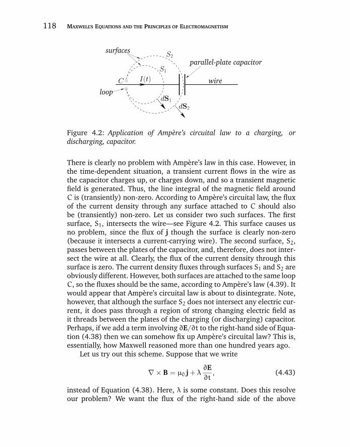
“chapter4” — 2007/11/29 — 13:54 — page 118 — #12
118 MAXWELL’S EQUATIONS AND THE PRINCIPLES OF ELECTROMAGNETISM
I(t)
dS2
dS1
S1
S2
⊗
C
parallel-plate capacitor
wire
surfaces
loop
Figure 4.2: Application of Ampere’s circuital law to a charging, ordischarging, capacitor.
There is clearly no problem with Ampere’s law in this case. However, inthe time-dependent situation, a transient current flows in the wire asthe capacitor charges up, or charges down, and so a transient magneticfield is generated. Thus, the line integral of the magnetic field aroundC is (transiently) non-zero. According to Ampere’s circuital law, the fluxof the current density through any surface attached to C should alsobe (transiently) non-zero. Let us consider two such surfaces. The firstsurface, S1, intersects the wire—see Figure 4.2. This surface causes usno problem, since the flux of j though the surface is clearly non-zero(because it intersects a current-carrying wire). The second surface, S2,passes between the plates of the capacitor, and, therefore, does not inter-sect the wire at all. Clearly, the flux of the current density through thissurface is zero. The current density fluxes through surfaces S1 and S2 areobviously different. However, both surfaces are attached to the same loopC, so the fluxes should be the same, according to Ampere’s law (4.39). Itwould appear that Ampere’s circuital law is about to disintegrate. Note,however, that although the surface S2 does not intersect any electric cur-rent, it does pass through a region of strong changing electric field asit threads between the plates of the charging (or discharging) capacitor.Perhaps, if we add a term involving ∂E/∂t to the right-hand side of Equa-tion (4.38) then we can somehow fix up Ampere’s circuital law? This is,essentially, how Maxwell reasoned more than one hundred years ago.
Let us try out this scheme. Suppose that we write
∇ × B = µ0 j + λ∂E∂t, (4.43)
instead of Equation (4.38). Here, λ is some constant. Does this resolveour problem? We want the flux of the right-hand side of the above
“chapter4” — 2007/11/29 — 13:54 — page 119 — #13
CHAPTER 4 TIME-DEPENDENT MAXWELL EQUATIONS 119
equation through some loop C to be well-defined; i.e., it should onlydepend on C, and not the particular surface S (which spans C) uponwhich it is evaluated. This is another way of saying that we want thedivergence of the right-hand side to be zero. In fact, we can see that thisis necessary for self-consistency, since the divergence of the left-handside is automatically zero. So, taking the divergence of Equation (4.43),we obtain
0 = µ0∇ · j + λ∂∇ · E∂t
. (4.44)
But, we know that
∇ · E =ρ
ε0, (4.45)
so combining the previous two equations we arrive at
µ0∇ · j +λ
ε0
∂ρ
∂t= 0. (4.46)
Now, our charge conservation law (4.42) can be written
∇ · j +∂ρ
∂t= 0. (4.47)
The previous two equations are in agreement provided λ = ε0µ0. So, ifwe modify the final Maxwell equation such that it reads
∇ × B = µ0 (j + jd), (4.48)
where
jd = ε0∂E∂t, (4.49)
then we find that the divergence of the right-hand side is zero as aconsequence of charge conservation. The extra term, jd, is called thedisplacement current density (this name was invented by Maxwell). Insummary, we have shown that although the flux of the real current den-sity through a loop is not well-defined, if we form the sum of the realcurrent density and the displacement current density then the flux of thisnew quantity through a loop is well-defined.
Of course, the displacement current is not a current at all. It is, infact, associated with the induction of magnetic fields by time-varyingelectric fields. Maxwell came up with this rather curious name because
“chapter4” — 2007/11/29 — 13:54 — page 120 — #14
120 MAXWELL’S EQUATIONS AND THE PRINCIPLES OF ELECTROMAGNETISM
many of his ideas regarding electric and magnetic fields were completelywrong. For instance, Maxwell believed in the ether (a tenuous invisiblemedium permeating all space), and he thought that electric and mag-netic fields were some sort of stresses in this medium. He also thoughtthat the displacement current was associated with displacements of theether (hence, the name). The reason that these misconceptions did notinvalidate his equations is quite simple. Maxwell based his equations onthe results of experiments, and he added in his extra term so as to makethese equations mathematically self-consistent. Both of these steps arevalid irrespective of the existence or non-existence of the ether.
Now, the field equations (4.35)–(4.38) are derived directly from theresults of famous nineteenth-century experiments. So, if a new terminvolving the time derivative of the electric field needs to be added toone of these equations, for the sake of mathematical consistency, why isthere is no corresponding nineteenth-century experimental result whichdemonstrates this fact? Well, it turns out that the new term describesan effect which is far too small to have been observed in the nineteenthcentury. Let us demonstrate this.
First, we shall show that it is comparatively easy to detect theinduction of an electric field by a changing magnetic field in a desk-top laboratory experiment. The Earth’s magnetic field is about 1 gauss(that is, 10−4 tesla). Magnetic fields generated by electromagnets (whichwill fit on a laboratory desktop) are typically about one hundred timesbigger than this. Let us, therefore, consider a hypothetical experiment inwhich a 100 gauss magnetic field is switched on suddenly. Suppose thatthe field ramps up in one tenth of a second. What electromotive force isgenerated in a 10 centimeter square loop of wire located in this field?Faraday’s law is written
V = −∂
∂t
∮B · dS ∼
BA
t, (4.50)
where B = 0.01 tesla is the field-strength, A = 0.01 m2 is the area ofthe loop, and t = 0.1 seconds is the ramp time. It follows that V ∼ 1
millivolt. Well, one millivolt is easily detectable. In fact, most hand-heldlaboratory voltmeters are calibrated in millivolts. It is, thus, clear that wewould have no difficulty whatsoever detecting the magnetic inductionof electric fields in a nineteenth-century-style laboratory experiment.
Let us now consider the electric induction of magnetic fields. Sup-pose that our electric field is generated by a parallel plate capacitor ofspacing one centimeter which is charged up to 100 volts. This gives a fieldof 104 volts per meter. Suppose, further, that the capacitor is discharged
“chapter4” — 2007/11/29 — 13:54 — page 121 — #15
CHAPTER 4 TIME-DEPENDENT MAXWELL EQUATIONS 121
in one tenth of a second. The law of electric induction is obtained by inte-grating Equation (4.48), and neglecting the first term on the right-handside. Thus, ∮
B · dl = ε0µ0∂
∂t
∫E · dS. (4.51)
Let us consider a loop 10 centimeters square. What is the magnetic fieldgenerated around this loop (which we could try to measure with a Hallprobe)? Very approximately, we find that
l B ∼ ε0µ0E l2
t, (4.52)
where l = 0.1 meters is the dimensions of the loop, B is the magneticfield-strength, E = 104 volts per meter is the electric field, and t = 0.1
seconds is the decay time of the field. We obtain B ∼ 10−9 gauss. Moderntechnology is unable to detect such a small magnetic field, so we cannotreally blame nineteenth-century physicists for not discovering electricinduction experimentally.
Note, however, that the displacement current is detectable in somemodern experiments. Suppose that we take an FM radio signal, amplifyit so that its peak voltage is one hundred volts, and then apply it to theparallel plate capacitor in the previous hypothetical experiment. Whatsize of magnetic field would this generate? Well, a typical FM signal oscil-lates at 109 Hz, so t in the previous example changes from 0.1 seconds to10−9 seconds. Thus, the induced magnetic field is about 10−1 gauss. Thisis certainly detectable by modern technology. Hence, we conclude thatif the electric field is oscillating sufficiently rapidly then electric induc-tion of magnetic fields is an observable effect. In fact, there is a virtuallyinfallible rule for deciding whether or not the displacement current canbe neglected in Equation (4.48). If electromagnetic radiation is importantthen the displacement current must be included. On the other hand, ifelectromagnetic radiation is unimportant then the displacement currentcan be safely neglected. Clearly, Maxwell’s inclusion of the displacementcurrent in Equation (4.48) was a vital step in his later realization thathis equations allowed propagating wave-like solutions. These solutionsare, of course, electromagnetic waves. But, more of this later.
We are now in a position to write out the full set of Maxwellequations:
∇ · E =ρ
ε0, (4.53)
∇ · B = 0, (4.54)
“chapter4” — 2007/11/29 — 13:54 — page 122 — #16
122 MAXWELL’S EQUATIONS AND THE PRINCIPLES OF ELECTROMAGNETISM
∇ × E = −∂B∂t, (4.55)
∇ × B = µ0 j + ε0µ0∂E∂t. (4.56)
These four partial differential equations constitute a complete descrip-tion of the behavior of electric and magnetic fields. The first equationdescribes how electric fields are induced by electric charges. The sec-ond equation says that there is no such thing as a magnetic monopole.The third equation describes the induction of electric fields by chang-ing magnetic fields, and the fourth equation describes the generationof magnetic fields by electric currents, and the induction of magneticfields by changing electric fields. Note that, with the inclusion of thedisplacement current, these equations treat electric and magnetic fieldson an equal footing: i.e., electric fields can induce magnetic fields, andvice versa. Equations (4.53)–(4.56) succinctly sum up the experimen-tal results of Coulomb, Ampere, and Faraday. They are called Maxwell’sequations because James Clerk Maxwell was the first to write them down(in component form). Maxwell also modified them so as to make themmathematically self-consistent.
As an example of a calculation involving the displacement current,let us find the current and displacement current densities associated withthe decaying charge distribution
ρ(r, t) =ρ0 exp(−t/τ)
r2 + a2, (4.57)
where r is a spherical polar coordinate, ρ0 is a constant, and τ and a arepositive constants. Now, according to charge conservation,
∇ · j = −∂ρ
∂t. (4.58)
By symmetry, we expect j = j(r, t). Hence, it follows that j = jr(r, t) er[since only a radial current has a non-zero divergence when j = j(r)].Hence, the above equation yields
1
r2∂(r2 jr)
∂r= −
∂ρ
∂t=ρ0 exp(−t/τ)
τ (r2 + a2). (4.59)
This expression can be integrated, subject to the sensible boundarycondition jr(0) = 0, to give
jr(r) =ρ0
τe−t/τ
[r− a tan−1(r/a)
r2
]. (4.60)

“chapter4” — 2007/11/29 — 13:54 — page 123 — #17
CHAPTER 4 TIME-DEPENDENT MAXWELL EQUATIONS 123
Now, the electric field generated by the decaying charge distributionsatisfies
∇ · E =ρ
ε0. (4.61)
Since ∂ρ/∂t = −ρ/τ, it can be seen, from a comparison of Equa-tions (4.58) and (4.61), that
E =τ
ε0j. (4.62)
However, the displacement current density is given by
jd = ε0∂E∂t
= −j, (4.63)
since ∂j/∂t = −j/τ. Hence, we conclude that the displacement currentdensity cancels out the true current density, so that j + jd = 0. This isjust as well, since ∇ × B = µ0 (j + jd). But, if B = B(r, t), by symmetry,then ∇ × B has no radial component—see Equation (2.169). Thus, if thecurrent and displacement current are constrained, by symmetry, to beradial, then they must sum to zero, else the fourth Maxwell equation can-not be satisfied. In fact, no magnetic field is generated in this particularexample, which also implies that there is no induced electric field.
4.6 POTENTIAL FORMULATION
We have seen that Equations (4.54) and (4.55) are automatically satis-fied if we write the electric and magnetic fields in terms of potentials: i.e.,
E = − ∇φ−∂A∂t, (4.64)
B = ∇ × A. (4.65)
This prescription is not unique, but we can make it unique by adoptingthe following conventions:
φ(r) → 0 as |r| → ∞, (4.66)
∇ · A = − ε0µ0∂φ
∂t. (4.67)
The above equations can be combined with Equation (4.53) to give
ε0µ0∂2φ
∂t2− ∇2φ =
ρ
ε0. (4.68)
“chapter4” — 2007/11/29 — 13:54 — page 124 — #18
124 MAXWELL’S EQUATIONS AND THE PRINCIPLES OF ELECTROMAGNETISM
Let us now consider Equation (4.56). Substitution of Equations(4.64) and (4.65) into this formula yields
∇ × ∇ × A ≡ ∇(∇ · A) − ∇2A = µ0 j − ε0µ0∂∇φ∂t
− ε0µ0∂2A∂t2
, (4.69)
or
ε0µ0∂2A∂t2
− ∇2A = µ0 j − ∇(
∇ · A + ε0µ0∂φ
∂t
). (4.70)
We can now see quite clearly where the Lorenz gauge condition (4.33)comes from. The above equation is, in general, very complicated, sinceit involves both the vector and scalar potentials. But, if we adopt theLorenz gauge then the last term on the right-hand side becomes zero,and the equation simplifies considerably, and ends up only involving thevector potential. Thus, we find that Maxwell’s equations reduce to thefollowing equations:
ε0µ0∂2φ
∂t2− ∇2φ =
ρ
ε0, (4.71)
ε0µ0∂2A∂t2
− ∇2A = µ0 j. (4.72)
Of course, this is the same (scalar) equation written four times over. Insteady-state (i.e., ∂/∂t = 0), the equation in question reduces to Poisson’sequation, which we know how to solve. With the ∂2/∂t2 terms included,it becomes a slightly more complicated equation (in fact, a driven three-dimensional wave equation).
4.7 ELECTROMAGNETIC WAVES
This is an appropriate point at which to demonstrate that Maxwell’sequations possess wave-like solutions which can propagate through avacuum. Let us start from Maxwell’s equations in free space (i.e., withno charges and no currents):
∇ · E = 0, (4.73)
∇ · B = 0, (4.74)
∇ × E = −∂B∂t, (4.75)
∇ × B = ε0µ0∂E∂t. (4.76)
“chapter4” — 2007/11/29 — 13:54 — page 125 — #19
CHAPTER 4 TIME-DEPENDENT MAXWELL EQUATIONS 125
Note that these equations exhibit a nice symmetry between the electricand magnetic fields.
There is an easy way to show that the above equations possess wave-like solutions, and a hard way. The easy way is to assume that thesolutions are going to be wave-like beforehand. Specifically, let us searchfor plane-wave solutions of the form:
E(r, t) = E0 cos (k · r −ωt), (4.77)
B(r, t) = B0 cos (k · r −ωt− φ). (4.78)
Here, E0 and B0 are constant vectors, k is called the wave-vector, andω is the angular frequency. The frequency in hertz, f, is related to theangular frequency viaω = 2π f. This frequency is conventionally definedto be positive. The quantity φ is a phase difference between the electricand magnetic fields. Actually, it is more convenient to write
E = E0 e i (k·r−ωt), (4.79)
B = B0 e i (k·r−ωt), (4.80)
where, by convention, the physical solution is the real part of the aboveequations. The phase difference φ is absorbed into the constant vectorB0 by allowing it to become complex. Thus, B0 → B0 e−iφ. In general,the vector E0 is also complex.
Now, a wave maximum of the electric field satisfies
k · r = ωt+ n2π, (4.81)
where n is an integer. The solution to this equation is a set of equallyspaced parallel planes (one plane for each possible value of n), whosenormals are parallel to the wave-vector k, and which propagate in thedirection of k with phase-velocity
v =ω
k. (4.82)
The spacing between adjacent planes (i.e., the wavelength) is given by
λ =2π
k(4.83)
—see Figure 4.3.Consider a general plane-wave vector field
A = A0 e i (k·r−ωt). (4.84)
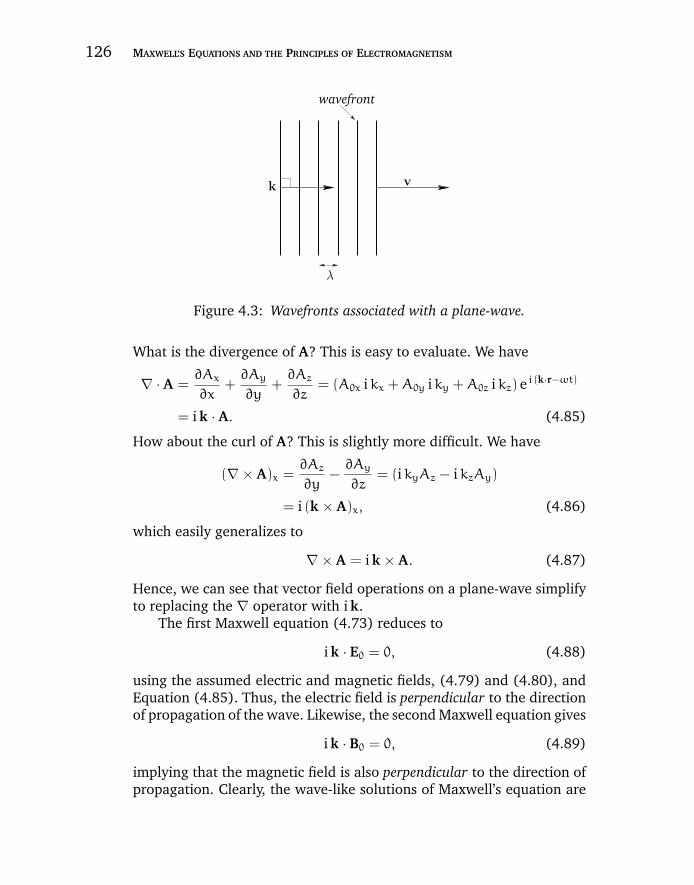
“chapter4” — 2007/11/29 — 13:54 — page 126 — #20
126 MAXWELL’S EQUATIONS AND THE PRINCIPLES OF ELECTROMAGNETISM
k v
λ
wavefront
Figure 4.3: Wavefronts associated with a plane-wave.
What is the divergence of A? This is easy to evaluate. We have
∇ · A =∂Ax
∂x+∂Ay
∂y+∂Az
∂z= (A0x i kx +A0y i ky +A0z i kz) e i (k·r−ωt)
= i k · A. (4.85)
How about the curl of A? This is slightly more difficult. We have
(∇ × A)x =∂Az
∂y−∂Ay
∂z= (i kyAz − i kzAy)
= i (k × A)x, (4.86)
which easily generalizes to
∇ × A = i k × A. (4.87)
Hence, we can see that vector field operations on a plane-wave simplifyto replacing the ∇ operator with i k.
The first Maxwell equation (4.73) reduces to
i k · E0 = 0, (4.88)
using the assumed electric and magnetic fields, (4.79) and (4.80), andEquation (4.85). Thus, the electric field is perpendicular to the directionof propagation of the wave. Likewise, the second Maxwell equation gives
i k · B0 = 0, (4.89)
implying that the magnetic field is also perpendicular to the direction ofpropagation. Clearly, the wave-like solutions of Maxwell’s equation are
“chapter4” — 2007/11/29 — 13:54 — page 127 — #21
CHAPTER 4 TIME-DEPENDENT MAXWELL EQUATIONS 127
a type of transverse wave. The third Maxwell equation yields
i k × E0 = iωB0, (4.90)
where use has been made of Equation (4.87). Dotting this equation withE0 gives
E0 · B0 =E0 · k × E0
ω= 0. (4.91)
Thus, the electric and magnetic fields are mutually perpendicular.Dotting equation (4.90) with B0 yields
B0 · k × E0 = ωB 20 > 0. (4.92)
Thus, the vectors E0, B0, and k are mutually perpendicular, and form aright-handed set. The final Maxwell equation gives
i k × B0 = −i ε0µ0 ωE0. (4.93)
Combining this with Equation (4.90) yields
k × (k × E0) = (k · E0) k − k2 E0 = −k2 E0 = −ε0µ0 ω2 E0, (4.94)
or
k2 = ε0µ0 ω2, (4.95)
where use has been made of Equation (4.88). However, we know, fromEquation (4.82), that the phase-velocity c is related to the magnitude ofthe wave-vector and the angular wave frequency via c = ω/k. Thus, weobtain
c =1√ε0µ0
. (4.96)
So, we have found transverse plane-wave solutions of the free-spaceMaxwell equations propagating at some phase-velocity c, which is givenby a combination of ε0 and µ0, and is thus the same for all frequenciesand wavelengths. The constants ε0 and µ0 are easily measurable. Theformer is related to the force acting between stationary electric charges,and the latter to the force acting between steady electric currents. Bothof these constants were fairly well-known in Maxwell’s time. Maxwell,incidentally, was the first person to look for wave-like solutions of his
“chapter4” — 2007/11/29 — 13:54 — page 128 — #22
128 MAXWELL’S EQUATIONS AND THE PRINCIPLES OF ELECTROMAGNETISM
equations, and, thus, to derive Equation (4.96). The modern values ofε0 and µ0 are
ε0 = 8.8542× 10⁻¹² C2 N−1 m−2, (4.97)
µ0 = 4π× 10−7 N A−2. (4.98)
Let us use these values to find the phase-velocity of “electromagneticwaves.” We obtain
c =1√ε0µ0
= 2.998× 10⁸ m s−1. (4.99)
Of course, we immediately recognize this as the velocity of light. Maxwellalso made this connection back in the 1870s. He conjectured that light,whose nature had previously been unknown, was a form of electromag-netic radiation. This was a remarkable prediction. After all, Maxwell’sequations were derived from the results of benchtop laboratory experi-ments involving charges, batteries, coils, and currents, which apparentlyhad nothing whatsoever to do with light.
Maxwell was able to make another remarkable prediction. The wave-length of light was well-known in the late nineteenth century fromstudies of diffraction through slits, etc. Visible light actually occupiesa surprisingly narrow wavelength range. The shortest wavelength bluelight which is visible has λ = 0.4 microns (one micron is 10−6 meters).The longest wavelength red light which is visible has λ = 0.76 microns.However, there is nothing in our analysis which suggests that this par-ticular range of wavelengths is special. Electromagnetic waves can haveany wavelength. Maxwell concluded that visible light was a small partof a vast spectrum of previously undiscovered types of electromagneticradiation. Since Maxwell’s time, virtually all of the non-visible parts ofthe electromagnetic spectrum have been observed.
Table 4.1 gives a brief guide to the electromagnetic spectrum. Elec-tromagnetic waves are of particular importance to us because they areour main source of information regarding the Universe around us. Radiowaves and microwaves (which are comparatively hard to scatter) haveprovided much of our knowledge about the center of our own galaxy.This is completely unobservable in visible light, which is strongly scat-tered by interstellar gas and dust lying in the galactic plane. For the samereason, the spiral arms of our galaxy can only be mapped out using radiowaves. Infrared radiation is useful for detecting protostars, which are notyet hot enough to emit visible radiation. Of course, visible radiation isstill the mainstay of Astronomy. Satellite-based ultraviolet observations

“chapter4” — 2007/11/29 — 13:54 — page 129 — #23
CHAPTER 4 TIME-DEPENDENT MAXWELL EQUATIONS 129
Radiation type Wavelength range (m)
Gamma Rays < 10−11
X-Rays 10−11–10−9
Ultraviolet 10−9–10−7
Visible 10−7–10−6
Infrared 10−6–10−4
Microwave 10−4–10−1
TV-FM 10−1–101
Radio > 101
Table 4.1 The electromagnetic spectrum.
have yielded invaluable insights into the structure and distribution of dis-tant galaxies. Finally, X-ray and γ-ray Astronomy usually concentrateson exotic objects, such as pulsars and supernova remnants.
Equations (4.88), (4.90), and the relation c = ω/k, imply that
B0 =E0
c. (4.100)
Thus, the magnetic field associated with an electromagnetic wave issmaller in magnitude than the electric field by a factor c. Consider a freecharge interacting with an electromagnetic wave. The force exerted onthe charge is given by the Lorentz formula
f = q (E + v × B). (4.101)
The ratio of the electric and magnetic forces is
fmagnetic
felectric∼vB0
E0∼v
c. (4.102)
So, unless the charge is moving close to the velocity of light (i.e., unlessthe charge is relativistic), the electric force greatly exceeds the magneticforce. Clearly, in most terrestrial situations, electromagnetic waves are anessentially electrical phenomenon (as far as their interaction with mattergoes). For this reason, electromagnetic waves are usually characterizedby their wave-vector k (which specifies the direction of propagation andthe wavelength) and the plane of polarization (i.e., the plane of oscil-lation) of the associated electric field. For a given wave-vector k, the
“chapter4” — 2007/11/29 — 13:54 — page 130 — #24
130 MAXWELL’S EQUATIONS AND THE PRINCIPLES OF ELECTROMAGNETISM
electric field can have any direction in the plane normal to k. How-ever, there are only two independent directions in a plane (i.e., we canonly define two linearly independent vectors in a plane). This impliesthat there are only two independent polarizations of an electromagneticwave, once its direction of propagation is specified.
But, how do electromagnetic waves propagate through a vacuum?After all, most types of wave require a medium before they can propagate(e.g., sound waves require air). The answer to this question is evidentfrom Equations (4.75) and (4.76). According to these equations, the timevariation of the electric component of the wave induces the magneticcomponent, and the time variation of the magnetic component inducesthe electric. In other words, electromagnetic waves are self-sustaining,and therefore require no medium through which to propagate.
Let us now search for the wave-like solutions of Maxwell’s equationsin free-space the hard way. Suppose that we take the curl of the fourthMaxwell equation, (4.76). We obtain
∇ × ∇ × B = ∇(∇ · B) − ∇2B = −∇2B = ε0µ0∂∇ × E∂t
. (4.103)
Here, we have made use of the fact that ∇ · B = 0. The third Maxwellequation, (4.75), yields (
∇2 −1
c2∂2
∂t2
)B = 0, (4.104)
where use has been made of Equation (4.99). A similar equation can beobtained for the electric field by taking the curl of Equation (4.75):(
∇2 −1
c2∂2
∂t2
)E = 0. (4.105)
We have found that electric and magnetic fields both satisfy equa-tions of the form (
∇2 −1
c2∂2
∂t2
)A = 0 (4.106)
in free space. As is easily verified, the most general solution to thisequation is
Ax = Fx(n · r − c t), (4.107)
Ay = Fy(n · r − c t), (4.108)
Az = Fz(n · r − c t), (4.109)

“chapter4” — 2007/11/29 — 13:54 — page 131 — #25
CHAPTER 4 TIME-DEPENDENT MAXWELL EQUATIONS 131
c t
Fx(r, t = 0) Fx(r, t = t)
r
Figure 4.4: An arbitrary wave-pulse.
where n is a unit vector, and Fx(φ), Fy(φ), and Fz(φ) are arbitrary one-dimensional scalar functions. Looking along the direction of n, so thatn · r = r, we find that
Ax = Fx(r− c t), (4.110)
Ay = Fy(r− c t), (4.111)
Az = Fz(r− c t). (4.112)
The x-component of this solution is shown schematically in Figure 4.4.It clearly propagates in r with velocity c. If we look along a directionwhich is perpendicular to n then n · r = 0, and there is no propagation.Thus, the components of A are arbitrarily shaped pulses which propagate,without changing shape, along the direction of n with velocity c. Thesepulses can be related to the sinusoidal plane-wave solutions which wefound earlier by Fourier transformation: e.g.,
Fx(r− c t) =1√2π
∫∞
−∞
Fx(k) e i k (r−c t) dk, (4.113)
where
Fx(k) =1√2π
∫∞
−∞
Fx(x) e−i k x dx. (4.114)
Thus, any arbitrary shaped pulse propagating in the direction of n withvelocity c can be broken down into a superposition of sinusoidal oscil-lations of different wavevectors, kn, propagating in the same directionwith the same velocity.
“chapter4” — 2007/11/29 — 13:54 — page 132 — #26
132 MAXWELL’S EQUATIONS AND THE PRINCIPLES OF ELECTROMAGNETISM
4.8 GREEN’S FUNCTIONS
The solution of the steady-state Maxwell equations essentially boils downto solving Poisson’s equation
∇2u = v, (4.115)
where v(r) is denoted the source function. The potential u(r) satisfiesthe boundary condition
u(r, t) → 0 as |r| → ∞, (4.116)
provided that the source function is reasonably localized. The solutionsto Poisson’s equation are superposable (because the equation is linear).This property is exploited in the Green’s function method of solving thisequation. The Green’s function G(r, r ′) is the potential generated by aunit amplitude point source, located at r ′, which satisfies the appropriateboundary conditions. Thus,
∇2G(r, r ′) = δ(r − r ′). (4.117)
Any source function v(r) can be represented as a weighted sum of pointsources
v(r) =
∫δ(r − r ′) v(r ′)d3r ′. (4.118)
It follows from superposability that the potential generated by the sourcev(r) can be written as the similarly weighted sum of point source drivenpotentials (i.e., Green’s functions)
u(r) =
∫G(r, r ′) v(r ′)d3r ′. (4.119)
We found earlier that the Green’s function for Poisson’s equation is
G(r, r ′) = −1
4π
1
|r − r ′|. (4.120)
It follows that the general solution to Equation (4.115) is written
u(r) = −1
4π
∫v(r ′)
|r − r ′|d3r ′. (4.121)
Note that the point source driven potential (4.120) is perfectly sensible.It is spherically symmetric about the source, and falls off smoothly withincreasing distance from the source.
“chapter4” — 2007/11/29 — 13:54 — page 133 — #27
CHAPTER 4 TIME-DEPENDENT MAXWELL EQUATIONS 133
The solution of the time-dependent Maxwell equations essentiallyboils down to solving the three-dimensional wave equation
(∇2 −
1
c2∂2
∂t2
)u = v, (4.122)
where v(r, t) is a time-varying source function. The potential u(r, t)satisfies the boundary conditions
u(r, t) → 0 as |r| → ∞ and |t| → ∞. (4.123)
The solutions to Equation (4.122) are superposable (since the equationis linear), so a Green’s function method of solution is again appropriate.The Green’s function G(r, r ′; t, t ′) is the potential generated by a pointimpulse located at position r ′ and applied at time t ′. Thus,
(∇2 −
1
c2∂2
∂t2
)G(r, r ′; t, t ′) = δ(r − r ′) δ(t− t ′). (4.124)
Of course, the Green’s function must satisfy the correct boundary con-ditions. A general source v(r, t) can be built up from a weighted sum ofpoint impulses
v(r, t) =
∫∫δ(r − r ′) δ(t− t ′) v(r ′, t ′)d3r ′ dt ′. (4.125)
It follows that the potential generated by v(r, t) can be written as thesimilarly weighted sum of point impulse driven potentials
u(r, t) =
∫∫G(r, r ′; t, t ′) v(r ′, t ′)d3r ′ dt ′. (4.126)
So, how do we find the Green’s function?Consider
G(r, r ′; t, t ′) =F(t− t ′ − |r − r ′|/c)
|r − r ′|, (4.127)
where F(φ) is a general scalar function. Let us try to prove the followingtheorem: (
∇2 −1
c2∂2
∂t2
)G = −4π F(t− t ′) δ(r − r ′). (4.128)

“chapter4” — 2007/11/29 — 13:54 — page 134 — #28
134 MAXWELL’S EQUATIONS AND THE PRINCIPLES OF ELECTROMAGNETISM
At a general point, r = r ′, the above expression reduces to(∇2 −
1
c2∂2
∂t2
)G = 0. (4.129)
Hence, we basically have to show that G is a valid solution of the free-space wave equation. Now, we can easily demonstrate that
∂|r − r ′|∂x
=x− x ′
|r − r ′|. (4.130)
It follows by simple differentiation that
∂2G
∂x2=
(3(x− x ′)2 − |r − r ′|2
|r − r ′|5
)F
+
(3(x− x ′)2 − |r − r ′|2
|r − r ′|4
)F ′
c+
(x− x ′)2
|r − r ′|3F ′′
c2, (4.131)
where F ′(φ) = dF(φ)/dφ, etc. We can derive analogous equations for∂2G/∂y2 and ∂2G/∂z2. Thus,
∇2G =∂2G
∂x2+∂2G
∂y2+∂2G
∂z2=
F ′′
|r − r ′| c2=1
c2∂2G
∂t2, (4.132)
giving (∇2 −
1
c2∂2
∂t2
)G = 0, (4.133)
which is the desired result. Consider, now, the region around r = r ′. It isclear that the dominant term on the right-hand side of Equation (4.131)as |r − r ′| → 0 is the first one, which is essentially F ∂2(|r − r ′|−1)/∂x2.It is also clear that (1/c2)(∂2G/∂t2) is negligible compared to this term.Thus, as |r − r ′| → 0 we find that(
∇2 −1
c2∂2
∂t2
)G → F(t− t ′)∇2
(1
|r − r ′|
). (4.134)
However, according to Equations (4.117) and (4.120),
∇2
(1
|r − r ′|
)= −4π δ(r − r ′). (4.135)
“chapter4” — 2007/11/29 — 13:54 — page 135 — #29
CHAPTER 4 TIME-DEPENDENT MAXWELL EQUATIONS 135
We conclude that(∇2 −
1
c2∂2
∂t2
)G = −4π F(t− t ′) δ(r − r ′), (4.136)
which is the desired result.Let us now make the special choice
F(φ) = −δ(φ)
4π. (4.137)
It follows from Equation (4.136) that(∇2 −
1
c2∂2
∂t2
)G = δ(r − r ′) δ(t− t ′). (4.138)
Thus,
G(r, r ′; t, t ′) = −1
4π
δ(t− t ′ − |r − r ′|/c)|r − r ′|
(4.139)
is the Green’s function for the driven wave equation (4.122).The time-dependent Green’s function (4.139) is the same as the
steady-state Green’s function (4.120), apart from the delta-functionappearing in the former. What does this delta-function do? Well, con-sider an observer at point r. Because of the delta-function, our observeronly measures a non-zero potential at one particular time
t = t ′ +|r − r ′|c
. (4.140)
It is clear that this is the time the impulse was applied at position r ′(i.e., t ′) plus the time taken for a light signal to travel between points r ′and r. At time t > t ′, the locus of all the points at which the potential isnon-zero is
|r − r ′| = c (t− t ′). (4.141)
In other words, it is a sphere centered on r ′ whose radius is the dis-tance traveled by light in the time interval since the impulse was appliedat position r ′. Thus, the Green’s function (4.139) describes a sphericalwave which emanates from position r ′ at time t ′, and propagates at thespeed of light. The amplitude of the wave is inversely proportional tothe distance from the source.
“chapter4” — 2007/11/29 — 13:54 — page 136 — #30
136 MAXWELL’S EQUATIONS AND THE PRINCIPLES OF ELECTROMAGNETISM
4.9 RETARDED POTENTIALS
We are now in a position to solve Maxwell’s equations. Recall that thesteady-state Maxwell equations reduce to
∇2φ = −ρ
ε0, (4.142)
∇2A = − µ0 j. (4.143)
The solutions to these equations are easily found using the Green’sfunction for Poisson’s equation, (4.120):
φ(r) =1
4πε0
∫ρ(r ′)
|r − r ′|d3r ′ (4.144)
A(r) =µ0
4π
∫j(r ′)
|r − r ′|d3r ′. (4.145)
The time-dependent Maxwell equations reduce to(∇2 −
1
c2∂2
∂t2
)φ = −
ρ
ε0, (4.146)
(∇2 −
1
c2∂2
∂t2
)A = − µ0 j. (4.147)
We can solve these equations using the time-dependent Green’s function,(4.139). From Equation (4.126), we find that
φ(r, t) =1
4πε0
∫∫δ(t− t ′ − |r − r ′|/c) ρ(r ′, t ′)
|r − r ′|d3r ′ dt ′, (4.148)
with a similar equation for A. Using the well-known property of delta-functions, these equations yield
φ(r, t) =1
4πε0
∫ρ(r ′, t− |r − r ′|/c)
|r − r ′|d3r ′ (4.149)
A(r, t) =µ0
4π
∫j(r ′, t− |r − r ′|/c)
|r − r ′|d3r ′. (4.150)
These are the general solutions to Maxwell’s equations. Note that thetime-dependent solutions, (4.149) and (4.150), are the same as thesteady-state solutions, (4.144) and (4.145), apart from the weird way inwhich time appears in the former. According to Equations (4.149) and(4.150), if we want to work out the potentials at position r and time t
“chapter4” — 2007/11/29 — 13:54 — page 137 — #31
CHAPTER 4 TIME-DEPENDENT MAXWELL EQUATIONS 137
then we have to perform integrals of the charge density and current den-sity over all space (just like in the steady-state situation). However, whenwe calculate the contribution of charges and currents at position r ′ tothese integrals we do not use the values at time t, instead we use thevalues at some earlier time t− |r − r ′|/c. What is this earlier time? It issimply the latest time at which a light signal emitted from position r ′would be received at position r before time t. This is called the retardedtime. Likewise, the potentials (4.149) and (4.150) are called retardedpotentials. It is often useful to adopt the following notation
A(r ′, t− |r − r ′|/c) ≡ [A(r ′, t)]. (4.151)
The square brackets denote retardation (i.e., using the retarded timeinstead of the real time). Using this notation Equations (4.149) and(4.150), become
φ(r) =1
4πε0
∫[ρ(r ′)]|r − r ′|
d3r ′, (4.152)
A(r) =µ0
4π
∫[j(r ′)]|r − r ′|
d3r ′. (4.153)
The time dependence in the above equations is taken as read.We are now in a position to understand electromagnetism at its most
fundamental level. A charge distribution ρ(r, t) can be thought of theo-retically as being built up out of a collection, or series, of charges whichinstantaneously come into existence, at some point r ′ and some time t ′,and then disappear again. Mathematically, this is written
ρ(r, t) =
∫∫δ(r − r ′)δ(t− t ′) ρ(r ′, t ′)d3r ′dt ′. (4.154)
Likewise, we can think of a current distribution j(r, t) as built up out of acollection, or series, of currents which instantaneously appear and thendisappear:
j(r, t) =
∫∫δ(r − r ′)δ(t− t ′) j(r ′, t ′)d3r ′dt ′. (4.155)
Each of these ephemeral charges and currents excites a spherical wavein the appropriate potential. Thus, the charge density at r ′ and t ′ sendsout a wave in the scalar potential:
φ(r, t) =ρ(r ′, t ′)4πε0
δ(t− t ′ − |r − r ′|/c)|r − r ′|
. (4.156)

“chapter4” — 2007/11/29 — 13:54 — page 138 — #32
138 MAXWELL’S EQUATIONS AND THE PRINCIPLES OF ELECTROMAGNETISM
Likewise, the current density at r ′ and t ′ sends out a wave in the vectorpotential:
A(r, t) =µ0 j(r ′, t ′)
4π
δ(t− t ′ − |r − r ′|/c)|r − r ′|
. (4.157)
These waves can be thought of as messengers which inform other chargesand currents about the charges and currents present at position r ′ andtime t ′. However, these messengers travel at a finite speed: i.e., thespeed of light. So, by the time they reach other charges and currentstheir message is a little out of date. Every charge and every currentin the Universe emits these spherical waves. The resultant scalar andvector potential fields are given by Equations (4.152) and (4.153). Ofcourse, we can turn these fields into electric and magnetic fields usingEquations (4.64) and (4.65). We can then evaluate the force exerted oncharges using the Lorentz formula. We can see that we have now escapedfrom the apparent action at a distance nature of Coulomb’s law andthe Biot-Savart law. Electromagnetic information is carried by sphericalwaves in the vector and scalar potentials, and, therefore, travels at thevelocity of light. Thus, if we change the position of a charge then a distantcharge can only respond after a time delay sufficient for a spherical waveto propagate from the former to the latter charge.
Consider a thought experiment in which a charge q appears atposition r0 at time t1, persists for a while, and then disappears attime t2. What is the electric field generated by such a charge? UsingEquation (4.150), we find that
φ(r, t) =q
4πε0
1
|r − r0|for t1 ≤ t− |r − r0|/c ≤ t2
= 0 otherwise. (4.158)
Now, E = −∇φ (since there are no currents, and therefore no vectorpotential is generated), so
E(r, t) =q
4πε0
r − r0|r − r0|3
for t1 ≤ t− |r − r0|/c ≤ t2
= 0 otherwise. (4.159)
This solution is shown pictorially in Figure 4.5. We can see that the chargeeffectively emits a Coulomb electric field which propagates radially awayfrom the charge at the speed of light. Likewise, it is easy to show thata current-carrying wire effectively emits an Amperian magnetic field atthe speed of light.

“chapter4” — 2007/11/29 — 13:54 — page 139 — #33
CHAPTER 4 TIME-DEPENDENT MAXWELL EQUATIONS 139
t2 < tt < t1 t1 < t < t2
Figure 4.5: Electric field due to a charge which appears at t = t1 anddisappears at t = t2.
We can now appreciate the essential difference between time-dependent electromagnetism and the action-at-a-distance laws ofCoulomb and Biot-Savart. In the latter theories, the field-lines act ratherlike rigid wires attached to charges (or circulating around currents).If the charges (or currents) move then so do the field-lines, leadinginevitably to unphysical action at a distance-type behavior. In the time-dependent theory, charges act rather like water sprinklers: i.e., they sprayout the Coulomb field in all directions at the speed of light. Similarly,current-carrying wires throw out magnetic field loops at the speed oflight. If we move a charge (or current) then field-lines emitted before-hand are not affected, so the field at a distant charge (or current) onlyresponds to the change in position after a time delay sufficient for thefield to propagate between the two charges (or currents) at the speedof light.
As we mentioned previously, it is not entirely obvious that electricand magnetic fields have a real existence in Coulomb’s law and the Biot-Savart law. After all, the only measurable quantities are the forces actingbetween charges and currents. We can certainly describe the force ona given charge or current, due to the other charges and currents in theUniverse, in terms of the local electric and magnetic fields, but we haveno way of knowing whether these fields persist when the charge or cur-rent is not present (i.e., we could argue that electric and magnetic fieldsare just a convenient way of calculating forces, but, in reality, the forcesare transmitted directly between charges and currents by some formof magic). On the other hand, it is patently obvious that electric and
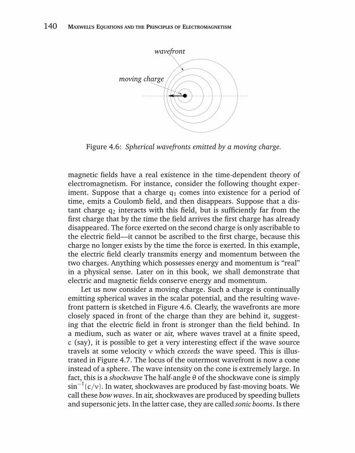
“chapter4” — 2007/11/29 — 13:54 — page 140 — #34
140 MAXWELL’S EQUATIONS AND THE PRINCIPLES OF ELECTROMAGNETISM
wavefront
moving charge
Figure 4.6: Spherical wavefronts emitted by a moving charge.
magnetic fields have a real existence in the time-dependent theory ofelectromagnetism. For instance, consider the following thought exper-iment. Suppose that a charge q1 comes into existence for a period oftime, emits a Coulomb field, and then disappears. Suppose that a dis-tant charge q2 interacts with this field, but is sufficiently far from thefirst charge that by the time the field arrives the first charge has alreadydisappeared. The force exerted on the second charge is only ascribable tothe electric field—it cannot be ascribed to the first charge, because thischarge no longer exists by the time the force is exerted. In this example,the electric field clearly transmits energy and momentum between thetwo charges. Anything which possesses energy and momentum is “real”in a physical sense. Later on in this book, we shall demonstrate thatelectric and magnetic fields conserve energy and momentum.
Let us now consider a moving charge. Such a charge is continuallyemitting spherical waves in the scalar potential, and the resulting wave-front pattern is sketched in Figure 4.6. Clearly, the wavefronts are moreclosely spaced in front of the charge than they are behind it, suggest-ing that the electric field in front is stronger than the field behind. Ina medium, such as water or air, where waves travel at a finite speed,c (say), it is possible to get a very interesting effect if the wave sourcetravels at some velocity v which exceeds the wave speed. This is illus-trated in Figure 4.7. The locus of the outermost wavefront is now a coneinstead of a sphere. The wave intensity on the cone is extremely large. Infact, this is a shockwave The half-angle θ of the shockwave cone is simplysin−1(c/v). In water, shockwaves are produced by fast-moving boats. Wecall these bow waves. In air, shockwaves are produced by speeding bulletsand supersonic jets. In the latter case, they are called sonic booms. Is there
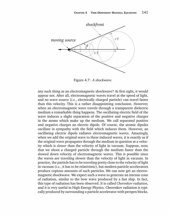
“chapter4” — 2007/11/29 — 13:54 — page 141 — #35
CHAPTER 4 TIME-DEPENDENT MAXWELL EQUATIONS 141
shockfront
c t
v t
θ
moving source
Figure 4.7: A shockwave.
any such thing as an electromagnetic shockwave? At first sight, it wouldappear not. After all, electromagnetic waves travel at the speed of light,and no wave source (i.e., electrically charged particle) can travel fasterthan this velocity. This is a rather disappointing conclusion. However,when an electromagnetic wave travels through a transparent dielectricmedium a remarkable thing happens. The oscillating electric field of thewave induces a slight separation of the positive and negative chargesin the atoms which make up the medium. We call separated positiveand negative charges an electric dipole. Of course, the atomic dipolesoscillate in sympathy with the field which induces them. However, anoscillating electric dipole radiates electromagnetic waves. Amazingly,when we add the original wave to these induced waves, it is exactly as ifthe original wave propagates through the medium in question at a veloc-ity which is slower than the velocity of light in vacuum. Suppose, now,that we shoot a charged particle through the medium faster than theslowed down velocity of electromagnetic waves. This is possible sincethe waves are traveling slower than the velocity of light in vacuum. Inpractice, the particle has to be traveling pretty close to the velocity of lightin vacuum (i.e., it has to be relativistic), but modern particle acceleratorsproduce copious amounts of such particles. We can now get an electro-magnetic shockwave. We expect such a wave to generate an intense coneof radiation, similar to the bow wave produced by a fast ship. In fact,this type of radiation has been observed. It is called Cherenkov radiation,and it is very useful in High-Energy Physics. Cherenkov radiation is typi-cally produced by surrounding a particle accelerator with perspex blocks.
“chapter4” — 2007/11/29 — 13:54 — page 142 — #36
142 MAXWELL’S EQUATIONS AND THE PRINCIPLES OF ELECTROMAGNETISM
Relativistic charged particles emanating from the accelerator passthrough the perspex traveling faster than the local velocity of light, andtherefore emit Cherenkov radiation. We know the velocity of light (c∗,say) in perspex (this can be worked out from the refractive index), so ifwe can measure the half angle θ of the Cherenkov radiation cone emit-ted by each particle then we can evaluate the particle speed v via thegeometric relation sin θ = c∗/v.
4.10 ADVANCED POTENTIALS?
We have defined the retarded time
tr = t− |r − r ′|/c (4.160)
as the latest time at which a light signal emitted from position r ′ wouldreach position r before time t. We have also shown that the solution toMaxwell’s equations can be written in terms of retarded potentials:
φ(r, t) =1
4πε0
∫ρ(r ′, tr)|r − r ′|
d3r ′, (4.161)
etc. But, is this the most general solution? Suppose that we define theadvanced time.
ta = t+ |r − r ′|/c. (4.162)
This is the time a light signal emitted at time t from position r wouldreach position r ′. It turns out that we can also write a solution toMaxwell’s equations in terms of advanced potentials:
φ(r, t) =1
4πε0
∫ρ(r ′, ta)|r − r ′|
d3r ′, (4.163)
etc. In fact, mathematically speaking, this is just as good a solution toMaxwell’s equation as the one involving retarded potentials. Considerthe Green’s function corresponding to our retarded potential solution:
φ(r, t) =ρ(r ′, t ′)4πε0
δ(t− t ′ − |r − r ′|/c)|r − r ′|
, (4.164)
with a similar equation for the vector potential. This says that the chargedensity present at position r ′ and time t ′ emits a spherical wave in the
“chapter4” — 2007/11/29 — 13:54 — page 143 — #37
CHAPTER 4 TIME-DEPENDENT MAXWELL EQUATIONS 143
scalar potential which propagates forward in time. The Green’s functioncorresponding to our advanced potential solution is
φ(r, t) =ρ(r ′, t ′)4πε0
δ(t− t ′ + |r − r ′|/c)|r − r ′|
. (4.165)
This says that the charge density present at position r ′ and time t ′ emitsa spherical wave in the scalar potential which propagates backward intime. Obviously, the advanced solution is usually rejected, on physicalgrounds, because it violates causality (i.e., it allows effects to exist priorto causes).
Now, the wave equation for the scalar potential,(∇2 −
1
c2∂2
∂t2
)φ = −
ρ
ε0, (4.166)
is manifestly symmetric in time (i.e., it is invariant under the trans-formation t → −t). Thus, mathematically speaking, backward-travelingwaves are just as good a solution to this equation as forward-travelingwaves. The equation is also symmetric in space (i.e., it is invariant underthe transformation r → −r). So, why do we adopt the Green’s function(4.164) which is symmetric in space (i.e., invariant under r → −r) butasymmetric in time (i.e., not invariant under t → −t)? Would it not bemore consistent to adopt the completely symmetric Green’s function
φ(r, t) =ρ(r ′, t ′)4πε0
1
2
(δ(t− t ′ − |r − r ′|/c)
|r − r ′|+δ(t− t ′ + |r − r ′|/c)
|r − r ′|
)?
(4.167)
According to this Green’s function, a given charge emits half of its wavesrunning forward in time (i.e., retarded waves), and the other half run-ning backward in time (i.e., advanced waves). This sounds completelycrazy! However, in the 1940s Richard P. Feynman and John A. Wheelerpointed out that under certain circumstances this prescription gives theright answer. Consider a charge interacting with “the rest of the Uni-verse,” where the “rest of the Universe” denotes all of the distant chargesin the Universe, and is, by implication, a very long way from our originalcharge. Suppose that the “rest of the Universe” is a perfect reflector ofadvanced waves and a perfect absorber of retarded waves. The wavesemitted by the charge can be written schematically as
F =1
2(retarded) +
1
2(advanced). (4.168)
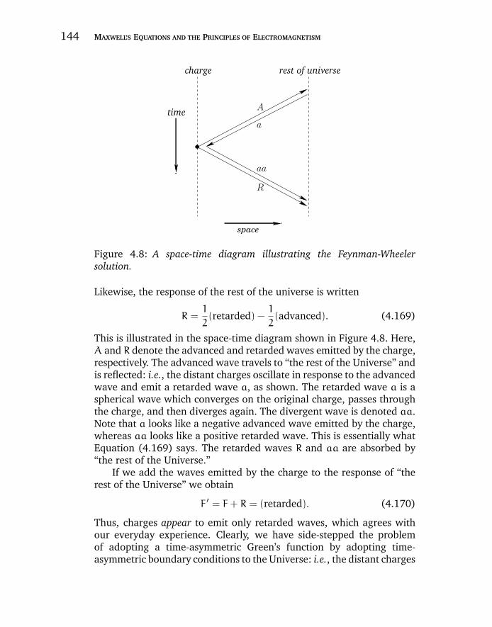
“chapter4” — 2007/11/29 — 13:54 — page 144 — #38
144 MAXWELL’S EQUATIONS AND THE PRINCIPLES OF ELECTROMAGNETISM
space
R
time
charge rest of universe
A
a
aa
Figure 4.8: A space-time diagram illustrating the Feynman-Wheelersolution.
Likewise, the response of the rest of the universe is written
R =1
2(retarded) −
1
2(advanced). (4.169)
This is illustrated in the space-time diagram shown in Figure 4.8. Here,A and R denote the advanced and retarded waves emitted by the charge,respectively. The advanced wave travels to “the rest of the Universe” andis reflected: i.e., the distant charges oscillate in response to the advancedwave and emit a retarded wave a, as shown. The retarded wave a is aspherical wave which converges on the original charge, passes throughthe charge, and then diverges again. The divergent wave is denoted aa.Note that a looks like a negative advanced wave emitted by the charge,whereas aa looks like a positive retarded wave. This is essentially whatEquation (4.169) says. The retarded waves R and aa are absorbed by“the rest of the Universe.”
If we add the waves emitted by the charge to the response of “therest of the Universe” we obtain
F ′ = F+ R = (retarded). (4.170)
Thus, charges appear to emit only retarded waves, which agrees withour everyday experience. Clearly, we have side-stepped the problemof adopting a time-asymmetric Green’s function by adopting time-asymmetric boundary conditions to the Universe: i.e., the distant charges
“chapter4” — 2007/11/29 — 13:54 — page 145 — #39
CHAPTER 4 TIME-DEPENDENT MAXWELL EQUATIONS 145
in the Universe absorb retarded waves and reflect advanced waves. Thisis possible because the absorption takes place at the end of the Universe,and the reflection takes place at the beginning of the Universe. It is quiteplausible that the state of the Universe (and, hence, its interaction withelectromagnetic waves) is completely different at these two epochs. Itshould be pointed out that the Feynman-Wheeler model runs into troublewhen an attempt is made to combine Electromagnetism with QuantumMechanics. These difficulties have yet to be resolved, so the present sta-tus of this model is that it is “an interesting idea,” but it is still not fullyaccepted into the canon of Physics.
4.11 RETARDED FIELDS
We have found the solution to Maxwell’s equations in terms of retardedpotentials. Let us now construct the associated retarded electric andmagnetic fields using
E = − ∇φ−∂A∂t, (4.171)
B = ∇ × A. (4.172)
It is helpful to write
R = r − r ′, (4.173)
where R = |r − r ′|. The retarded time becomes tr = t− R/c, and a gen-eral retarded quantity is written [F(r ′, t)] ≡ F(r ′, tr). Thus, we can writethe retarded potential solutions of Maxwell’s equations in the especiallycompact form:
φ(r, t) =1
4πε0
∫[ρ]
Rd3r ′, (4.174)
A(r, t) =µ0
4π
∫[j]Rd3r ′. (4.175)
It is easily seen that
∇φ =1
4πε0
∫ ([ρ]∇(R−1) +
[∂ρ/∂t]
R∇tr
)d3r ′
= −1
4πε0
∫ ([ρ]
R3R +
[∂ρ/∂t]
c R2R)d3r ′, (4.176)
“chapter4” — 2007/11/29 — 13:54 — page 146 — #40
146 MAXWELL’S EQUATIONS AND THE PRINCIPLES OF ELECTROMAGNETISM
where use has been made of
∇R =RR, ∇(R−1) = −
RR3, ∇tr = −
Rc R. (4.177)
Likewise,
∇ × A =µ0
4π
∫ (∇(R−1) × [j] +
∇tr × [∂j/∂t]R
)d3r ′
= −µ0
4π
∫ (R × [j]R3
+R × [∂j/∂t]
c R2
)d3r ′. (4.178)
Equations (4.171), (4.172), (4.176), and (4.178) can be combined togive
E =1
4πε0
∫ ([ρ]
RR3
+
[∂ρ
∂t
]Rc R2
−[∂j/∂t]c2 R
)d3r ′, (4.179)
which is the time-dependent generalization of Coulomb’s law, and
B =µ0
4π
∫ ([j] × RR3
+[∂j/∂t] × R
c R2
)d3r ′, (4.180)
which is the time-dependent generalization of the Biot-Savart law.Suppose that the typical variation time-scale of our charges and cur-
rents is t0. Let us define R0 = c t0, which is the distance a light ray travelsin time t0. We can evaluate Equations (4.179) and (4.180) in two asymp-totic limits: the near field region R R0, and the far field region R R0.In the near field region,
|t− tr|
t0=R
R0 1, (4.181)
so the difference between retarded time and standard time is relativelysmall. This allows us to expand retarded quantities in a Taylor series.Thus,
[ρ] ρ+∂ρ
∂t(tr − t) +
1
2
∂2ρ
∂t2(tr − t)2 + · · · , (4.182)
giving
[ρ] ρ−∂ρ
∂t
R
c+1
2
∂2ρ
∂t2R2
c2+ · · · . (4.183)
“chapter4” — 2007/11/29 — 13:54 — page 147 — #41
CHAPTER 4 TIME-DEPENDENT MAXWELL EQUATIONS 147
Expansion of the retarded quantities in the near field region yields
E(r, t) 1
4πε0
∫ (ρRR3
−1
2
∂2ρ
∂t2Rc2 R
−∂j/∂tc2 R
+ · · ·)d3r ′, (4.184)
B(r, t) µ0
4π
∫ (j × RR3
−1
2
(∂2j/∂t2) × Rc2 R
+ · · ·)d3r ′. (4.185)
In Equation (4.184), the first term on the right-hand side correspondsto Coulomb’s law, the second term is the lowest order correction toCoulomb’s law due to retardation effects, and the third term correspondsto Faraday induction. In Equation (4.185), the first term on the right-hand side is the Biot-Savart law, and the second term is the lowest ordercorrection to the Biot-Savart law due to retardation effects. Note thatthe retardation corrections are only of order (R/R0)
2. We might sup-pose, from looking at Equations (4.179) and (4.180), that the correctionsshould be of order R/R0. However, all of the order R/R0 terms canceledout in the previous expansion. Suppose, then, that we have an electriccircuit sitting on a laboratory benchtop. Let the currents in the circuitchange on a typical time-scale of one tenth of a second. In this time,light can travel about 3× 10⁷ meters, so R0 ∼ 30, 000 kilometers. Thelength-scale of the experiment is about one meter, so R = 1meter. Thus,the retardation corrections are of relative order (3× 10⁷)−2 ∼ 10−15. It isclear that we are fairly safe just using Coulomb’s law, Faraday’s law, andthe Biot-Savart law to analyze the fields generated by this type of circuit.
In the far field region, R R0, Equations (4.179) and (4.180) aredominated by the terms which vary like R−1, so that
E(r, t) −1
4πε0
∫[∂j⊥/∂t]c2 R
d3r ′, (4.186)
B(r, t) µ0
4π
∫[∂j⊥/∂t] × R
c R2d3r ′, (4.187)
where
j⊥ = j −(j · R)
R2R. (4.188)
Here, use has been made of [∂ρ/∂t] = −[∇ · j] and [∇ · j] −[∂j/∂t] ·R/cR. Suppose that our charges and currents are localized to some finiteregion of space in the vicinity of the origin, and that the extent of thecurrent-and-charge-containing region is much less than |r|. It follows that
“chapter4” — 2007/11/29 — 13:54 — page 148 — #42
148 MAXWELL’S EQUATIONS AND THE PRINCIPLES OF ELECTROMAGNETISM
retarded quantities can be written
[ρ(r ′, t)] ρ(r ′, t− r/c), (4.189)
etc. Thus, the electric field reduces to
E(r, t) −1
4πε0
[∫∂j⊥/∂t d3r ′]c2 r
, (4.190)
whereas the magnetic field is given by
B(r, t) 1
4πε0
[∫∂j⊥/∂t d3r ′]× r
c3 r2. (4.191)
Here, [· · · ] merely denotes evaluation at the retarded time t− r/c. Notethat
E
B= c, (4.192)
and
E · B = 0. (4.193)
This configuration of electric and magnetic fields is characteristic of anelectromagnetic wave (see Section 4.7). Thus, Equations (4.190) and(4.191) describe an electromagnetic wave propagating radially awayfrom the charge-and-current-containing region. Note that the wave isdriven by time-varying electric currents. Now, charges moving with aconstant velocity constitute a steady current, so a non-steady current isassociated with accelerating charges. We conclude that accelerating elec-tric charges emit electromagnetic waves. The wave fields, (4.190) and(4.191), fall off like the inverse of the distance from the wave source.This behavior should be contrasted with that of Coulomb or Biot-Savartfields, which fall off like the inverse square of the distance from thesource. It is the fact that wave fields attenuate fairly gently with increas-ing distance from the source which makes Astronomy possible. If wavefields obeyed an inverse square law then no appreciable radiation wouldreach us from the rest of the Universe.
In conclusion, electric and magnetic fields look simple in the nearfield region (they are just Coulomb fields, etc.) and also in the far fieldregion (they are just electromagnetic waves). Only in the intermediateregion, R ∼ R0, do things start to get really complicated (so we generallyavoid looking in this region!).
“chapter4” — 2007/11/29 — 13:54 — page 149 — #43
CHAPTER 4 TIME-DEPENDENT MAXWELL EQUATIONS 149
4.12 MAXWELL’S EQUATIONS
This marks the end of our theoretical investigation of Maxwell’s equa-tions. Let us now summarize what we have learned so far. The fieldequations which govern electric and magnetic fields are written:
∇ · E =ρ
ε0, (4.194)
∇ · B = 0, (4.195)
∇ × E = −∂B∂t, (4.196)
∇ × B = µ0 j +1
c2∂E∂t. (4.197)
These equations can be integrated to give∮S
E · dS =1
ε0
∫V
ρdV, (4.198)
∮S
B · dS = 0, (4.199)
∮C
E · dl = −∂
∂t
∫S
B · dS, (4.200)
∮C
B · dl = µ0
∫S ′
j · dS +1
c2∂
∂t
∫S ′
E · dS. (4.201)
Here, S is a surface enclosing a volume V, and S ′ a surface attached toa closed curve C.
Equations (4.195) and (4.196) are automatically satisfied by writing
E = − ∇φ−∂A∂t, (4.202)
B = ∇ × A. (4.203)
This prescription is not unique (there are many choices ofφ and A whichgenerate the same fields), but we can make it unique by adopting thefollowing conventions:
φ(r, t) → 0 as |r| → ∞, (4.204)
and
1
c2∂φ
∂t+ ∇ · A = 0. (4.205)
“chapter4” — 2007/11/29 — 13:54 — page 150 — #44
150 MAXWELL’S EQUATIONS AND THE PRINCIPLES OF ELECTROMAGNETISM
The latter convention is known as the Lorenz gauge condition. Equations(4.194) and (4.197) reduce to(
∇2 −1
c2∂2
∂t2
)φ = −
ρ
ε0, (4.206)
(∇2 −
1
c2∂2
∂t2
)A = −µ0 j. (4.207)
These are driven wave equations of the general form(∇2 −
1
c2∂2
∂t2
)u = v. (4.208)
The Green’s function for this equation which satisfies sensible boundaryconditions, and is consistent with causality, is
G(r, r ′; t, t ′) = −1
4π
δ(t− t ′ − |r − r ′|/c)|r − r ′|
. (4.209)
Thus, the solutions to Equations (4.206) and (4.207) are
φ(r, t) =1
4πε0
∫[ρ]
Rd3r ′, (4.210)
A(r, t) =µ0
4π
∫[j]Rd3r ′, (4.211)
where R = |r − r ′|, and [A] ≡ A(r ′, t− R/c). These solutions can becombined with Equations (4.202) and (4.203) to give
E(r, t) =1
4πε0
∫ ([ρ]
RR3
+
[∂ρ
∂t
]Rc R2
−[∂j/∂t]c2 R
)d3r ′, (4.212)
B(r, t) =µ0
4π
∫ ([j] × RR3
+[∂j/∂t] × R
c R2
)d3r ′. (4.213)
Equations (4.194)–(4.213) constitute the complete theory of clas-sical electromagnetism. We can express the same information in termsof field equations [Equations (4.194)–(4.197)], integrated field equa-tions [Equations (4.198)–(4.201)], retarded electromagnetic potentials[Equations (4.210) and (4.211)], and retarded electromagnetic fields[Equations (4.212) and (4.213)]. Let us now consider the applicationsof this theory.
“chapter4” — 2007/11/29 — 13:54 — page 151 — #45
CHAPTER 4 TIME-DEPENDENT MAXWELL EQUATIONS 151
4.13 EXERCISES
4.1. Consider a particle accelerator in which charged particles are constrained to
move in a circle in the x-y plane by a z-directed magnetic field. If the magnetic
field-strength is gradually increased then the particles are accelerated by the
induced electric field. This type of accelerator is called a betatron. It is preferable
to keep the radius of the particle orbit constant during the acceleration. Show
that this is possible provided that the magnetic field distribution is such that the
average field over the area of the orbit is twice the field at the circumference.
Assume that the field is symmetric about the center of the orbit, and that the
particles are subrelativistic.
4.2. A charged particle executes a circular orbit in the plane perpendicular to a uni-
form magnetic field of strength B. If the magnitude of the field is very gradually
increased then the induced electric field accelerates the charge. Demonstrate
that in a single rotation
∆K
K ∆B
B,
where K is the particle’s kinetic energy. Hence, deduce that the ratio K/B is
approximately constant during the field ramp. By considering the circulating
charge as a circular current loop, show that the charge’s effective magnetic
moment is
m =K
B,
and is, thus, approximately conserved during the field ramp. Does the radius of
the orbit increase or decrease as the magnetic field-strength increases?
4.3. Demonstrate that∫
V
jd3r =
∫
S
r j · dS −
∫
V
r ∇ · jd3r,
where S is a surface enclosing some volume V . Hence, deduce that for a
distribution of charges and currents localized to some finite region of space∫
jd3r =dpdt,
where the integral is over the whole volume of the distribution, and
p =
∫r ρd3r
is the distribution’s electric dipole moment.

“chapter4” — 2007/11/29 — 13:54 — page 152 — #46
152 MAXWELL’S EQUATIONS AND THE PRINCIPLES OF ELECTROMAGNETISM
4.4. Given that Ampere’s circuital law implies the Biot-Savart law, show that Faraday’s
law implies that
E(r, t) = −1
4π
∫[∂B(r ′, t)/∂t] × (r − r ′)
|r − r ′|3d3r ′.
Consider a thin iron ring of major radius a and minor cross-sectional area A. A
uniform circulating magnetic field B(t) is produced inside the iron by current
flowing in a wire wound toroidally onto the ring. Show that the electric field
induced on the major axis of the ring is
E(z, t) = −a2 A
2 (a2 + z2)3/2
(dB
dt
)ez,
where z is measured from the plane of the ring, in a right-handed sense with
respect to the circulating magnetic field. Demonstrate that∫
∞
−∞
Ez(z, t)dz = −AdB
dt.
Derive this result directly from Faraday’s law.
4.5. A Rogowski coil consists of a thin wire wound uniformly onto a non-magnetic
ring-shaped former of major radius a and constant cross-sectional area A. Sup-
pose that there are N turns around the ring. If a time-dependent current I(t)
passes anywhere through the ring show that the voltage induced in the wire is
V =µ0
2π
NA
a
dI
dt.
4.6. In a certain region of space the charge density takes the form
ρ = ρ0 e−λ r,
where r is a spherical polar coordinate, ρ0 a spatial constant, and λ a positive
constant. Find the electric field generated by this charge distribution. Suppose
that
ρ0 = ρ00 e−γ t,
where ρ00 is a spatial and temporal constant, and γ a positive constant. What
is the current density associated with the time-varying charge density? What
is the displacement current generated by the changing electric field? Find the
magnetic field generated by these current distributions.
4.7. An alternating current I = I0 cos(ωt) flows down a long straight wire of neg-
ligible thickness, and back along a thin co-axial conducting cylindrical shell of
radius R.
(a) In which direction does the induced electric field E point (radial, circum-
ferential, or longitudinal)?
“chapter4” — 2007/11/29 — 13:54 — page 153 — #47
CHAPTER 4 TIME-DEPENDENT MAXWELL EQUATIONS 153
(b) Find E as a function of r (perpendicular distance from the wire).
(c) Find the displacement current density jd.
(d) Integrate jd to obtain the total displacement current
Id =
∫jd · dS.
(e) What is the ratio of Id to I? If the outer cylinder were 2 mm in diameter,
how high would the frequency ω have to be (in Hz) for Id to be 1% of I?
4.8. Consider the one-dimensional free-space electromagnetic wave equation
∂2E
∂z2= ε0µ0
∂2E
∂t2,
where E is the electric field-strength in the x-direction. Show that a change of
variables,
α = t +√ε0µ0 z,
β = t −√ε0 µ0 z,
causes the equation to assume a form which can easily be integrated. Hence,
deduce that
E(z, t) = F(α) +G(β),
where F and G are arbitrary functions. Interpret this solution.
4.9. Given the free-space electromagnetic wave electric field
E = E0 cos[k (z − c t)] ex + E0 sin[k (z + c t)] ey,
where k is real, find the corresponding magnetic field B.
4.10. Given a plane electromagnetic wave propagating in free-space along the positive
z-direction, and polarized such that
E = E0 sin [k (z − c t)] ,
where k is real, and E0 is a constant vector, show that it is possible to set the
scalar potential φ to zero. Find a possible vector potential A which satisfies the
Lorenz gauge.
4.11. The electric field of a plane electromagnetic wave propagating in the z-direction
is written
E = A e i (k z−ω t) ex + B e i (k z−ω t) ey,
where A and B are complex numbers, and k and ω are positive real numbers.
Of course, the physical electric field is the real part of the above expression.
Suppose that
A = |E|/√2, B = A e i φ
,
“chapter4” — 2007/11/29 — 13:54 — page 154 — #48
154 MAXWELL’S EQUATIONS AND THE PRINCIPLES OF ELECTROMAGNETISM
where |E| is the maximum magnitude of the electric field vector, and φ is real.
Demonstrate that, in general, the tip of the electric field vector traces out an
ellipse in the x-y plane whose major axis is tilted at 45 with respect to the x-axis.
Show that the major/minor radii of the ellipse are |E| |cosφ/2| and |E| |sinφ/2|,
and that the electric field vector rotates clockwise (looking down the z-axis)
when 0 ≤ φ ≤ 180, and counterclockwise otherwise. Demonstrate that for the
special cases when φ = 0, 180, the electric field vector traces out a straight-
line, passing through the origin, in the x-y plane. These cases correspond to
so-called linearly polarized waves. Show that for the special cases when φ =
90, 270 the electric field vector traces out a circle in the x-y plane, rotating
clockwise and counterclockwise, respectively. These cases correspond to left-
hand and right-hand circularly polarized waves, respectively. (The handedness
is determined with respect to the direction of wave propagation and the sense
of rotation of the electric field in the plane perpendicular to this direction.)
Note that in the general case the electric field vector traces out an ellipse in the
x-y plane, rotating clockwise and counterclockwise, respectively, depending on
whether or not 0 ≤ φ ≤ 180. These cases correspond to left-hand and right-
hand elliptically polarized waves, respectively.
4.12. A magnetic monopole of monopole charge qm placed at the origin generates a
radial magnetic field of the form
Br(r) =µ0 c qm
4π r2.
Using this result, and assuming that the number of magnetic monopoles in the
Universe is a conserved quantity (like the number of electric charges), show
that when Maxwell’s equations are generalized to take magnetic monopoles
into account they take the form
∇ · E =ρ
ε0,
∇ · H =ρm
ε0,
∇ × E = − µ0c jm −∂H∂τ,
∇ × H = µ0c j +∂E∂τ,
where H = cB and τ = c t. Here, ρm is the number density of monopoles, and
jm is the monopole current density.
4.13. Consider a distribution of charges and currents which is localized in a region of
linear extent a in the vicinity of the origin. Demonstrate that the lowest order
“chapter4” — 2007/11/29 — 13:54 — page 155 — #49
CHAPTER 4 TIME-DEPENDENT MAXWELL EQUATIONS 155
electric and magnetic field generated by such a distribution in the far field region,
|r| a, is
E(r, t) −1
4πε0 c2ee × ([p] × er)
r,
B(r, t) 1
4πε0 c3[p] × err
,
where er = r/r, p =∫
r ρd3r is the electric dipole moment of the distribution,
and _ denotes a time derivative. Here, [· · · ] implies evaluation at the retarded
time t − r/c. Suppose that p = p0 cos(ωt) ez. Show that the far field electric
and magnetic fields take the form
E(r, t) = −ω2 p0
4πε0 c2cos[ω (t − r/c)]
sin θr
eθ,
B(r, t) = −ω2 p0
4πε0 c3cos[ω (t − r/c)]
sin θr
eφ.
Here, θ and φ are spherical polar coordinates.

“chapter4” — 2007/11/29 — 13:54 — page 156 — #50
“chapter5” — 2007/11/29 — 15:40 — page 157 — #1
C h a p t e r 5 ELECTROSTATICCALCULATIONS
5.1 INTRODUCTION
In this chapter, we shall make a detailed investigation of the electric fieldsgenerated by stationary charge distributions using Maxwell’s equations.In particular, we shall examine the interaction of electrostatic fields withohmic conductors.
5.2 ELECTROSTATIC ENERGY
Consider a collection ofN static point charges qi located at position vec-tors ri, respectively (where i runs from 1 toN). What is the electrostaticenergy stored in such a collection? In other words, how much workwould we have to do in order to assemble the charges, starting from aninitial state in which they are all at rest and very widely separated?
Well, we know that a static electric field is conservative, and canconsequently be written in terms of a scalar potential:
E = −∇φ. (5.1)
We also know that the electric force on a charge q located at position ris written
f = qE(r). (5.2)
The work we would have to do against electrical forces in order to slowlymove the charge from point P to point Q is simply
W = −
∫QP
f · dl = −q
∫QP
E · dl = q
∫QP
∇φ · dl = q [φ(Q) − φ(P)] .
(5.3)The negative sign in the above expression comes about because we wouldhave to exert a force −f on the charge, in order to counteract the forceexerted by the electric field. Recall, finally, that the scalar potential field
157
“chapter5” — 2007/11/29 — 15:40 — page 158 — #2
158 MAXWELL’S EQUATIONS AND THE PRINCIPLES OF ELECTROMAGNETISM
generated by a point charge q located at position r ′ is
φ(r) =1
4πε0
q
|r − r ′|. (5.4)
Let us build up our collection of charges one by one. It takes no workto bring the first charge from infinity, since there is no electric field tofight against. Let us clamp this charge in position at r1. In order to bringthe second charge into position at r2, we have to do work against theelectric field generated by the first charge. According to Equations (5.3)and Equations (5.4), this work is given by
W2 =1
4πε0
q2 q1
|r2 − r1|. (5.5)
Let us now bring the third charge into position. Since electric fields andscalar potentials are superposable, the work done whilst moving the thirdcharge from infinity to r3 is simply the sum of the works done againstthe electric fields generated by charges 1 and 2 taken in isolation:
W3 =1
4πε0
(q3 q1
|r3 − r1|+
q3 q2
|r3 − r2|
). (5.6)
Thus, the total work done in assembling the three charges is given by
W =1
4πε0
(q2 q1
|r2 − r1|+
q3 q1
|r3 − r1|+
q3 q2
|r3 − r2|
). (5.7)
This result can easily be generalized to N charges:
W =1
4πε0
N∑i=1
N∑j<i
qi qj
|ri − rj|. (5.8)
The restriction that j must be less than i makes the above summationrather messy. If we were to sum without restriction (other than j = i)then each pair of charges would be counted twice. It is convenient to dojust this, and then to divide the result by two. Thus, we obtain
W =1
2
1
4πε0
N∑i=1
N∑j=1j=i
qi qj
|ri − rj|. (5.9)
This is the potential energy (i.e., the difference between the total energyand the kinetic energy) of a collection of charges. We can think of this
“chapter5” — 2007/11/29 — 15:40 — page 159 — #3
CHAPTER 5 ELECTROSTATIC CALCULATIONS 159
quantity as the work required to bring stationary charges from infinityand assemble them in the required formation. Alternatively, it is thekinetic energy which would be released if the collection were dissolved,and the charges returned to infinity. But where is this potential energystored? Let us investigate further.
Equation (5.9) can be written
W =1
2
N∑i=1
qi φi, (5.10)
where
φi =1
4πε0
N∑j=1j=i
qj
|ri − rj|(5.11)
is the scalar potential experienced by the ith charge due to the othercharges in the distribution.
Let us now consider the potential energy of a continuous chargedistribution. It is tempting to write
W =1
2
∫ρφd3r, (5.12)
by analogy with Equations (5.10) and (5.11), where
φ(r) =1
4πε0
∫ρ(r ′)
|r − r ′|d3r ′ (5.13)
is the familiar scalar potential generated by a continuous charge distribu-tion of charge density ρ(r). Let us try this out. We know from Maxwell’sequations that
ρ = ε0∇·E, (5.14)
so Equation (5.12) can be written
W =ε0
2
∫φ∇·Ed3r. (5.15)
Now, vector field theory yields the standard result
∇ · (Eφ) = φ∇·E + E·∇φ. (5.16)
“chapter5” — 2007/11/29 — 15:40 — page 160 — #4
160 MAXWELL’S EQUATIONS AND THE PRINCIPLES OF ELECTROMAGNETISM
However, ∇φ = −E, so we obtain
W =ε0
2
[∫∇·(Eφ)d3r +
∫E2 d3r
]. (5.17)
Application of Gauss’ theorem gives
W =ε0
2
(∮S
φE · dS +
∫V
E2 dV
), (5.18)
where V is some volume which encloses all of the charges, and S is itsbounding surface. Let us assume that V is a sphere, centered on theorigin, and let us take the limit in which the radius r of this sphere goesto infinity. We know that, in general, the electric field at large distancesfrom a bounded charge distribution looks like the field of a point charge,and, therefore, falls off like 1/r2. Likewise, the potential falls off like1/r—see Exercise 3.7. However, the surface area of the sphere increaseslike r2. Hence, it is clear that, in the limit as r → ∞, the surface integralin Equation (5.18) falls off like 1/r, and is consequently zero. Thus,Equation (5.18) reduces to
W =ε0
2
∫E2 d3r, (5.19)
where the integral is over all space. This is a very interesting result. Ittells us that the potential energy of a continuous charge distribution isstored in the electric field generated by the distribution. Of course, wenow have to assume that an electric field possesses an energy density
U =ε0
2E2. (5.20)
We can easily check that Equation (5.19) is correct. Suppose that wehave a chargeQwhich is uniformly distributed within a sphere of radiusa centered on the origin. Let us imagine building up this charge distribu-tion from a succession of thin spherical layers of infinitesimal thickness.At each stage, we gather a small amount of charge dq from infinity, andspread it over the surface of the sphere in a thin layer extending fromr to r+ dr. We continue this process until the final radius of the sphereis a. If q(r) is the sphere’s charge when it has attained radius r, then thework done in bringing a charge dq to its surface is
dW =1
4πε0
q(r)dq
r. (5.21)
This follows from Equation (5.5), since the electric field generated out-side a spherical charge distribution is the same as that of a point charge
“chapter5” — 2007/11/29 — 15:40 — page 161 — #5
CHAPTER 5 ELECTROSTATIC CALCULATIONS 161
q(r) located at its geometric center (r = 0)—see Section 3.4. If theconstant charge density of the sphere is ρ then
q(r) =4π
3r3 ρ, (5.22)
and
dq = 4π r2 ρ dr. (5.23)
Thus, Equation (5.21) becomes
dW =4π
3ε0ρ2 r4 dr. (5.24)
The total work needed to build up the sphere from nothing to radius ais plainly
W =4π
3ε0ρ2
∫a0
r4 dr =4π
15ε0ρ2 a5. (5.25)
This can also be written in terms of the total charge Q = (4π/3)a3 ρ as
W =3
5
Q2
4πε0 a. (5.26)
Now that we have evaluated the potential energy of a sphericalcharge distribution by the direct method, let us work it out using Equa-tion (5.19). We shall assume that the electric field is both radial andspherically symmetric, so that E = Er(r) er. Application of Gauss’ law,∮
S
E · dS =1
ε0
∫V
ρdV, (5.27)
where V is a sphere of radius r, centered on the origin, gives
Er(r) =Q
4πε0
r
a3(5.28)
for r < a, and
Er(r) =Q
4πε0 r2(5.29)
for r ≥ a. Equations (5.19), (5.28), and (5.29) yield
W =Q2
8πε0
(1
a6
∫a0
r4 dr+
∫∞
a
dr
r2
), (5.30)
“chapter5” — 2007/11/29 — 15:40 — page 162 — #6
162 MAXWELL’S EQUATIONS AND THE PRINCIPLES OF ELECTROMAGNETISM
which reduces to
W =Q2
8πε0 a
(1
5+ 1
)=3
5
Q2
4πε0 a. (5.31)
Thus, Equation (5.19) gives the correct answer.The reason that we have checked Equation (5.19) so carefully is that,
on close inspection, it is found to be inconsistent with Equation (5.10),from which it was supposedly derived! For instance, the energy givenby Equation (5.19) is manifestly positive definite, whereas the energygiven by Equation (5.10) can be negative (it is certainly negative for acollection of two point charges of opposite sign). The inconsistency wasintroduced into our analysis when we replaced Equation (5.11) withEquation (5.13). In Equation (5.11), the self-interaction of the ith chargewith its own electric field is specifically excluded, whereas it is includedin Equation (5.13). Thus, the potential energies (5.10) and (5.19) aredifferent because in the former we start from ready-made point charges,whereas in the latter we build up the whole charge distribution fromscratch. Hence, if we were to work out the potential energy of a pointcharge distribution using Equation (5.19) then we would obtain theenergy (5.10) plus the energy required to assemble the point charges.What is the energy required to assemble a point charge? In fact, it isinfinite. To see this, let us suppose, for the sake of argument, that ourpoint charges actually consist of charge uniformly distributed in smallspheres of radius b. According to Equation (5.26), the energy requiredto assemble the ith point charge is
Wi =3
5
q2i4πε0 b
. (5.32)
We can think of this as the self-energy of the ith charge. Thus, we canwrite
W =ε0
2
∫E2 d3r =
1
2
N∑i=1
qi φi +
N∑i=1
Wi (5.33)
which enables us to reconcile Equations (5.10) and (5.19). Unfortu-nately, if our point charges really are point charges then b → 0, and theself-energy of each charge becomes infinite. Thus, the potential energiespredicted by Equations (5.10) and (5.19) differ by an infinite amount.What does this all mean? We have to conclude that the idea of locatingelectrostatic potential energy in the electric field is inconsistent with the
“chapter5” — 2007/11/29 — 15:40 — page 163 — #7
CHAPTER 5 ELECTROSTATIC CALCULATIONS 163
existence of point charges. One way out of this difficulty would be to saythat elementary charges, such as electrons, are not points objects, butinstead have finite spatial extents. Regrettably, there is no experimentalevidence to back up this assertion. Alternatively, we could say that ourclassical theory of electromagnetism breaks down on very small length-scales due to quantum effects. Unfortunately, the quantum mechanicalversion of electromagnetism (which is called Quantum Electrodynamics)suffers from the same infinities in the self-energies of charged particles asthe classical version. There is a prescription, called renormalization, forsteering round these infinities, and getting finite answers which agreewith experimental data to extraordinary accuracy. However, nobodyreally understands why this prescription works. Indeed, the problemof the infinite self-energies of elementary charged particles is still anunresolved issue in Physics.
5.3 OHM’S LAW
A conductor is a medium which contains free electric charges (usuallyelectrons) which drift in the presence of an applied electric field, givingrise to an electric current flowing in the same direction as the field. Thewell-known relationship between the current and the voltage in a typicalconductor is given by Ohm’s law: i.e.,
V = I R, (5.34)
where V is the voltage drop across a conductor of electrical resis-tance R through which a current I flows. Incidentally, the unit ofelectrical resistance is the ohm (Ω), which is equivalent to a volt perampere.
Let us generalize Ohm’s law so that it is expressed in terms of E andj, rather than V and I. Consider a length l of a conductor of uniformcross-sectional area A through which a current I flows. In general, weexpect the electrical resistance of the conductor to be proportional toits length, l, and inversely proportional to its cross-sectional area, A(i.e., we expect that it is harder to push an electrical current down along rather than a short wire, and easier to push a current down a widerather than a narrow conducting channel). Thus, we can write
R = ηl
A. (5.35)

“chapter5” — 2007/11/29 — 15:40 — page 164 — #8
164 MAXWELL’S EQUATIONS AND THE PRINCIPLES OF ELECTROMAGNETISM
Here, the constant η is called the resistivity of the conducting medium,and is measured in units of ohm-meters. Hence, Ohm’s law becomes
V = ηl
AI. (5.36)
However, I/A = jz (supposing that the conductor is aligned along thez-axis) and V/l = Ez, so the above equation reduces to
Ez = η jz. (5.37)
There is nothing special about the z-axis (in an isotropic conductingmedium), so the previous formula immediately generalizes to
E = η j. (5.38)
This is the vector form of Ohm’s law.It is fairly easy to account for the above equation physically. Con-
sider a metal which has n free electrons per unit volume. Of course,the metal also has a fixed lattice of metal ions whose charge per unitvolume is equal and opposite to that of the free electrons, renderingthe medium electrically neutral. In the presence of an electric field E,a given free electron accelerates (from rest at t = 0) such that its driftvelocity is written v = −(e/me) tE, where −e is the electron charge, andme the electron mass. Suppose that, on average, a drifting electron col-lides with a metal ion once every τ seconds. Given that a metal ion ismuch more massive than an electron, we expect a free electron to loseall of the momentum it had previously acquired from the electric fieldduring such a collision. It follows that the mean drift velocity of thefree electrons is v = −(e τ/2me) E. Hence, the mean current density isj = (ne2 τ/2me) E. Thus, the resistivity can be written
η =ne2 τ
2me. (5.39)
We conclude that the resistivity of a typical conducting medium isdetermined by the number density of free electrons, as well as themean collision rate of these electrons with the fixed ions. The fact thatj ∝ E leads immediately to the relation (5.35) between resistivity andresistance.
A free charge q which moves through a voltage drop V acquires anenergy qV from the electric field. In a conducting medium, this energyis dissipated as heat (the conversion to heat takes place each time a freecharge collides with a fixed ion). This type of heating is called ohmic
“chapter5” — 2007/11/29 — 15:40 — page 165 — #9
CHAPTER 5 ELECTROSTATIC CALCULATIONS 165
heating. Suppose thatN charges per unit time pass through a conductor.The current flowing is obviously I = Nq. The total energy gained by thecharges, which appears as heat inside the conductor, is
P = NqV = I V (5.40)
per unit time. Thus, the heating power is
P = I V = I2 R =V2
R. (5.41)
Equations (5.40) and (5.41) generalize to
P = j · E = η j2, (5.42)
where P is now the power dissipated per unit volume inside theconducting medium.
5.4 CONDUCTORS
Most (but not all) electrical conductors obey Ohm’s law. Such conductorsare termed ohmic. Suppose that we apply an electric field to an ohmicconductor. What is going to happen? According to Equation (5.38),the electric field drives currents. These currents redistribute the chargeinside the conductor until the original electric field is canceled out. Atthis point, the currents stop flowing. It might be objected that the cur-rents could keep flowing in closed loops. According to Ohm’s law, thiswould require a non-zero emf,
∮E · dl, acting around each loop (unless
the conductor is a superconductor, with η = 0). However, we know thatin a steady-state ∮
C
E · dl = 0 (5.43)
around any closed loop C. This proves that a steady-state emf actingaround a closed loop inside a conductor is impossible. The only otheralternative is
j = E = 0 (5.44)
everywhere inside the conductor. It immediately follows from theMaxwell equation ∇ · E = ρ/ε0 that
ρ = 0. (5.45)

“chapter5” — 2007/11/29 — 15:40 — page 166 — #10
166 MAXWELL’S EQUATIONS AND THE PRINCIPLES OF ELECTROMAGNETISM
So, there are no electric charges in the interior of a conductor. But,how can a conductor cancel out an applied electric field if it contains nocharges? The answer is that all of the charges reside on the surface ofthe conductor. In reality, the charges lie within one or two atomic layersof the surface (see any textbook on solid-state physics). The differencein scalar potential between two points P and Q is simply
φ(Q) − φ(P) =
∫QP
∇φ · dl = −
∫QP
E · dl. (5.46)
However, if P and Q both lie inside the same conductor then it is clearfrom Equations (5.44) and (5.46) that the potential difference betweenP andQ is zero. This is true no matter where P andQ are situated insidethe conductor, so we conclude that the scalar potential must be uniforminside a conductor. A corollary of this is that the surface of a conductoris an equipotential (i.e., φ = constant) surface.
So, the electric field inside a conductor is zero. We can demonstratethat the field within an empty cavity lying inside a conductor is zero aswell, provided that there are no charges within the cavity. Let us, firstof all, apply Gauss’ law to a surface S which surrounds the cavity, butlies wholly within the conducting medium—see Figure 5.1. Since theelectric field is zero inside a conductor, it follows that zero net chargeis enclosed by S. This does not preclude the possibility that there areequal amounts of positive and negative charges distributed on the innersurface of the conductor. However, we can easily rule out this possibilityusing the steady-state relation∮
C
E · dl = 0, (5.47)
for any closed loop C. If there are any electric field-lines inside thecavity then they must run from the positive to the negative surfacecharges. Consider a closed loop C which straddles the cavity and theconductor, such as the one shown in Figure 5.1. In the presence offield-lines, it is clear that the line integral of E along that portion of theloop which lies inside the cavity is non-zero. However, the line integralof E along that portion of the loop which runs through the conductingmedium is obviously zero (since E = 0 inside a conductor). Thus, theline integral of the field around the closed loop C is non-zero, whichclearly contradicts Equation (5.47). In fact, this equation implies thatthe line integral of the electric field along any path which runs throughthe cavity, from one point on the interior surface of the conductor to
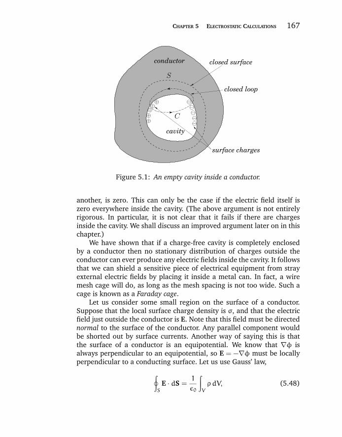
“chapter5” — 2007/11/29 — 15:40 — page 167 — #11
CHAPTER 5 ELECTROSTATIC CALCULATIONS 167
closed surface
surface charges
closed loop
cavity
conductor
⊕⊕
S
C
⊕⊕⊕
Figure 5.1: An empty cavity inside a conductor.
another, is zero. This can only be the case if the electric field itself iszero everywhere inside the cavity. (The above argument is not entirelyrigorous. In particular, it is not clear that it fails if there are chargesinside the cavity. We shall discuss an improved argument later on in thischapter.)
We have shown that if a charge-free cavity is completely enclosedby a conductor then no stationary distribution of charges outside theconductor can ever produce any electric fields inside the cavity. It followsthat we can shield a sensitive piece of electrical equipment from strayexternal electric fields by placing it inside a metal can. In fact, a wiremesh cage will do, as long as the mesh spacing is not too wide. Such acage is known as a Faraday cage.
Let us consider some small region on the surface of a conductor.Suppose that the local surface charge density is σ, and that the electricfield just outside the conductor is E. Note that this field must be directednormal to the surface of the conductor. Any parallel component wouldbe shorted out by surface currents. Another way of saying this is thatthe surface of a conductor is an equipotential. We know that ∇φ isalways perpendicular to an equipotential, so E = −∇φ must be locallyperpendicular to a conducting surface. Let us use Gauss’ law,
∮S
E · dS =1
ε0
∫V
ρdV, (5.48)
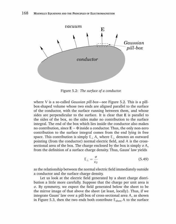
“chapter5” — 2007/11/29 — 15:40 — page 168 — #12
168 MAXWELL’S EQUATIONS AND THE PRINCIPLES OF ELECTROMAGNETISM
Gaussian
conductor
vacuum
pill-box
E
Figure 5.2: The surface of a conductor.
where V is a so-called Gaussian pill-box—see Figure 5.2. This is a pill-box-shaped volume whose two ends are aligned parallel to the surfaceof the conductor, with the surface running between them, and whosesides are perpendicular to the surface. It is clear that E is parallel tothe sides of the box, so the sides make no contribution to the surfaceintegral. The end of the box which lies inside the conductor also makesno contribution, since E = 0 inside a conductor. Thus, the only non-zerocontribution to the surface integral comes from the end lying in freespace. This contribution is simply E⊥A, where E⊥ denotes an outwardpointing (from the conductor) normal electric field, and A is the cross-sectional area of the box. The charge enclosed by the box is simply σA,from the definition of a surface charge density. Thus, Gauss’ law yields
E⊥ =σ
ε0(5.49)
as the relationship between the normal electric field immediately outsidea conductor and the surface charge density.
Let us look at the electric field generated by a sheet charge distri-bution a little more carefully. Suppose that the charge per unit area isσ. By symmetry, we expect the field generated below the sheet to bethe mirror image of that above the sheet (at least, locally). Thus, if weintegrate Gauss’ law over a pill-box of cross-sectional area A, as shownin Figure 5.3, then the two ends both contribute EsheetA to the surface
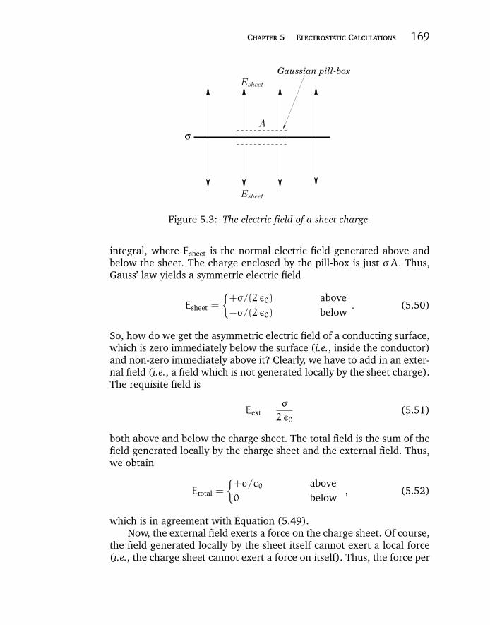
“chapter5” — 2007/11/29 — 15:40 — page 169 — #13
CHAPTER 5 ELECTROSTATIC CALCULATIONS 169
Gaussian pill-box .
Esheet
A
σ
Esheet
Figure 5.3: The electric field of a sheet charge.
integral, where Esheet is the normal electric field generated above andbelow the sheet. The charge enclosed by the pill-box is just σA. Thus,Gauss’ law yields a symmetric electric field
Esheet =
+σ/(2 ε0) above−σ/(2 ε0) below
. (5.50)
So, how do we get the asymmetric electric field of a conducting surface,which is zero immediately below the surface (i.e., inside the conductor)and non-zero immediately above it? Clearly, we have to add in an exter-nal field (i.e., a field which is not generated locally by the sheet charge).The requisite field is
Eext =σ
2 ε0(5.51)
both above and below the charge sheet. The total field is the sum of thefield generated locally by the charge sheet and the external field. Thus,we obtain
Etotal =
+σ/ε0 above0 below
, (5.52)
which is in agreement with Equation (5.49).Now, the external field exerts a force on the charge sheet. Of course,
the field generated locally by the sheet itself cannot exert a local force(i.e., the charge sheet cannot exert a force on itself). Thus, the force per
“chapter5” — 2007/11/29 — 15:40 — page 170 — #14
170 MAXWELL’S EQUATIONS AND THE PRINCIPLES OF ELECTROMAGNETISM
unit area acting on the surface of a conductor always acts outward, andis given by
p = σEext =σ2
2 ε0. (5.53)
We conclude that there is an electrostatic pressure acting on any chargedconductor. This effect can be observed by charging up soap bubbles: theadditional electrostatic pressure eventually causes them to burst. Theelectrostatic pressure can also be written
p =ε0
2E2⊥, (5.54)
where E⊥ is the field-strength immediately above the surface of theconductor. Note that, according to the above formula, the electrostaticpressure is equivalent to the energy density of the electric field imme-diately outside the conductor. This is not a coincidence. Suppose thatthe conductor expands normally by an average distance dx, due to theelectrostatic pressure. The electric field is excluded from the region intowhich the conductor expands. The volume of this region is dV = Adx,where A is the surface area of the conductor. Thus, the energy of theelectric field decreases by an amount dE = UdV = (ε0/2)E
2⊥ dV, where
U is the energy density of the field. This decrease in energy can beascribed to the work which the field does on the conductor in order tomake it expand. This work is dW = pAdx, where p is the force per unitarea that the field exerts on the conductor. Thus, dE = dW, from energyconservation, giving
p =ε0
2E2⊥. (5.55)
Incidentally, this technique for calculating a force, given an expressionfor the energy of a system as a function of some adjustable parameter, iscalled the principle of virtual work.
We have seen that an electric field is excluded from the inside of aconductor, but not from the outside, giving rise to a net outward force.We can account for this fact by saying that the field exerts a negativepressure (ε0/2)E
2⊥ on the conductor. Now, we know that if we evacuate
a closed metal can then the pressure difference between the inside andthe outside eventually causes it to implode. Likewise, if we place thecan in a strong electric field then the pressure difference between theinside and the outside will eventually cause it to explode. How big afield do we need before the electrostatic pressure difference is the same
“chapter5” — 2007/11/29 — 15:40 — page 171 — #15
CHAPTER 5 ELECTROSTATIC CALCULATIONS 171
as that obtained by evacuating the can? In other words, what electricfield exerts a negative pressure of one atmosphere (i.e., 105 newtons permeter squared) on the can? The answer is a field of strength E ∼ 108 voltsper meter. Fortunately, this is a rather large electric field, so there is nodanger of your car exploding when you turn on the radio!
5.5 BOUNDARY CONDITIONS ON THE ELECTRIC FIELD
What are the general boundary conditions satisfied by the electric fieldat the interface between two different media: e.g., the interface betweena vacuum and a conductor? Consider an interface P between two media1 and 2. Let us, first of all, apply Gauss’ law,∮
S
E · dS =1
ε0
∫V
ρdV, (5.56)
to a Gaussian pill-box S of cross-sectional area A whose two ends arelocally parallel to the interface—see Figure 5.4. The ends of the box canbe made arbitrarily close together. In this limit, the flux of the electricfield out of the sides of the box is obviously negligible, and the onlycontribution to the flux comes from the two ends. In fact,∮
S
E · dS = (E⊥ 1 − E⊥ 2)A, (5.57)
where E⊥ 1 is the perpendicular (to the interface) electric field in medium1 at the interface, etc. The charge enclosed by the pill-box is simplyσA, where σ is the sheet charge density on the interface. Note that anyvolume distribution of charge gives rise to a negligible contribution tothe right-hand side of Equation (5.56), in the limit where the two endsof the pill-box are very closely spaced. Thus, Gauss’ law yields
E⊥ 1 − E⊥ 2 =σ
ε0(5.58)
at the interface: i.e., the presence of a charge sheet on an interfacecauses a discontinuity in the perpendicular component of the electricfield. What about the parallel electric field? Let us apply Faraday’s lawto a rectangular loop C whose long sides, length l, run parallel to theinterface, ∮
C
E · dl = −∂
∂t
∫S
B · dS (5.59)
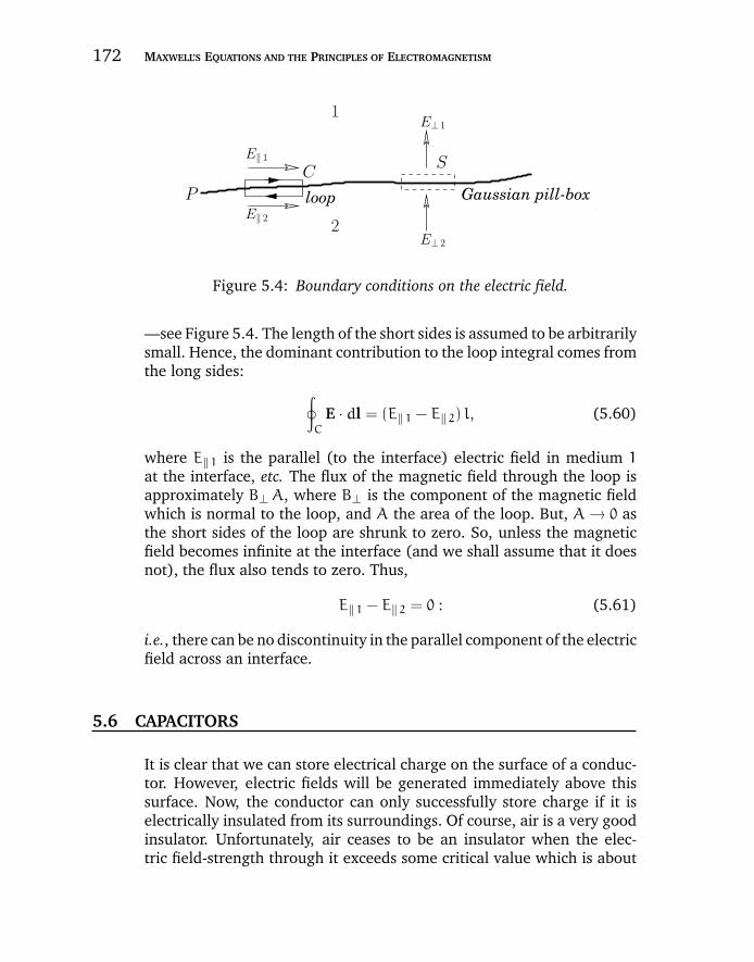
“chapter5” — 2007/11/29 — 15:40 — page 172 — #16
172 MAXWELL’S EQUATIONS AND THE PRINCIPLES OF ELECTROMAGNETISM
loop Gaussian pill-box.
2
P
SC
E‖ 1
E‖ 2
E⊥ 1
E⊥ 2
1
Figure 5.4: Boundary conditions on the electric field.
—see Figure 5.4. The length of the short sides is assumed to be arbitrarilysmall. Hence, the dominant contribution to the loop integral comes fromthe long sides: ∮
C
E · dl = (E‖ 1 − E‖ 2) l, (5.60)
where E‖ 1 is the parallel (to the interface) electric field in medium 1
at the interface, etc. The flux of the magnetic field through the loop isapproximately B⊥A, where B⊥ is the component of the magnetic fieldwhich is normal to the loop, and A the area of the loop. But, A → 0 asthe short sides of the loop are shrunk to zero. So, unless the magneticfield becomes infinite at the interface (and we shall assume that it doesnot), the flux also tends to zero. Thus,
E‖ 1 − E‖ 2 = 0 : (5.61)
i.e., there can be no discontinuity in the parallel component of the electricfield across an interface.
5.6 CAPACITORS
It is clear that we can store electrical charge on the surface of a conduc-tor. However, electric fields will be generated immediately above thissurface. Now, the conductor can only successfully store charge if it iselectrically insulated from its surroundings. Of course, air is a very goodinsulator. Unfortunately, air ceases to be an insulator when the elec-tric field-strength through it exceeds some critical value which is about
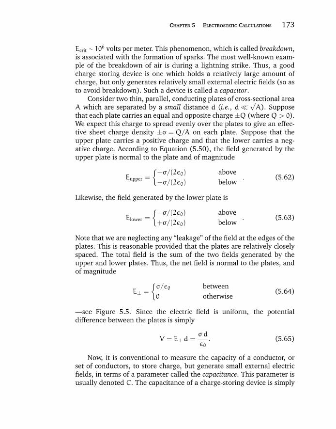
“chapter5” — 2007/11/29 — 15:40 — page 173 — #17
CHAPTER 5 ELECTROSTATIC CALCULATIONS 173
Ecrit ∼ 106 volts per meter. This phenomenon, which is called breakdown,is associated with the formation of sparks. The most well-known exam-ple of the breakdown of air is during a lightning strike. Thus, a goodcharge storing device is one which holds a relatively large amount ofcharge, but only generates relatively small external electric fields (so asto avoid breakdown). Such a device is called a capacitor.
Consider two thin, parallel, conducting plates of cross-sectional areaA which are separated by a small distance d (i.e., d √
A). Supposethat each plate carries an equal and opposite charge ±Q (whereQ > 0).We expect this charge to spread evenly over the plates to give an effec-tive sheet charge density ±σ = Q/A on each plate. Suppose that theupper plate carries a positive charge and that the lower carries a neg-ative charge. According to Equation (5.50), the field generated by theupper plate is normal to the plate and of magnitude
Eupper =
+σ/(2ε0) above−σ/(2ε0) below
. (5.62)
Likewise, the field generated by the lower plate is
Elower =
−σ/(2ε0) above+σ/(2ε0) below
. (5.63)
Note that we are neglecting any “leakage” of the field at the edges of theplates. This is reasonable provided that the plates are relatively closelyspaced. The total field is the sum of the two fields generated by theupper and lower plates. Thus, the net field is normal to the plates, andof magnitude
E⊥ =
σ/ε0 between0 otherwise
(5.64)
—see Figure 5.5. Since the electric field is uniform, the potentialdifference between the plates is simply
V = E⊥ d =σd
ε0. (5.65)
Now, it is conventional to measure the capacity of a conductor, orset of conductors, to store charge, but generate small external electricfields, in terms of a parameter called the capacitance. This parameter isusually denoted C. The capacitance of a charge-storing device is simply
“chapter5” — 2007/11/29 — 15:40 — page 174 — #18
174 MAXWELL’S EQUATIONS AND THE PRINCIPLES OF ELECTROMAGNETISM
conducting plates
A
d E⊥
σ
σ
Figure 5.5: The electric field of a parallel plate capacitor.
the ratio of the charge stored to the potential difference generated bythis charge: i.e.,
C =Q
V. (5.66)
Clearly, a good charge-storing device has a high capacitance. Incidentally,capacitance is measured in farads (F), which are equivalent to coulombsper volt. This is a rather unwieldy unit, since capacitors in electricalcircuits typically have capacitances which are only about one millionthof a farad. For a parallel plate capacitor, we have
C =σA
V=ε0 A
d. (5.67)
Note that the capacitance only depends on geometric quantities, such asthe area and spacing of the plates. This is a consequence of the superpos-ability of electric fields. If we double the charge on a set of conductorsthen we double the electric fields generated around them, and we, there-fore, double the potential difference between the conductors. Thus, thepotential difference between the conductors is always directly propor-tional to the charge on the conductors: the constant of proportionality(the inverse of the capacitance) can only depend on geometry.
Suppose that the charge ±Q on each plate of a parallel plate capac-itor is built up gradually by transferring small amounts of charge fromone plate to another. If the instantaneous charge on the plates is ±q,and an infinitesimal amount of positive charge dq is transferred fromthe negatively charged to the positively charge plate, then the work
“chapter5” — 2007/11/29 — 15:40 — page 175 — #19
CHAPTER 5 ELECTROSTATIC CALCULATIONS 175
done is dW = V dq = qdq/C, where V is the instantaneous voltagedifference between the plates. Note that the voltage difference is suchthat it opposes any increase in the charge on either plate. The total workdone in charging the capacitor is
W =1
C
∫Q0
qdq =Q2
2C=1
2CV2, (5.68)
where use has been made of Equation (5.66). The energy stored in thecapacitor is the same as the work required to charge up the capacitor.Thus, the stored energy is
W =1
2CV2. (5.69)
This is a general result which holds for all types of capacitor.The energy of a charged parallel plate capacitor is actually stored
in the electric field between the plates. This field is of approximatelyconstant magnitude E⊥ = V/d, and occupies a region of volume Ad.Thus, given the energy density of an electric field, U = (ε0/2)E
2, theenergy stored in the electric field is
W =ε0
2
V2
d2Ad =
1
2CV2, (5.70)
where use has been made of Equation (5.67). Note that Equations (5.68)and (5.70) agree with one another. The fact that the energy of a capacitoris stored in its electric field is also a general result.
The idea, which we discussed earlier, that an electric field exerts anegative pressure (ε0/2)E
2⊥ on conductors immediately suggests that the
two plates in a parallel plate capacitor attract one another with a mutualforce
F =ε0
2E 2
⊥ A =1
2
CV2
d. (5.71)
It is not actually necessary to have two oppositely charged conduc-tors in order to make a capacitor. Consider an isolated conducting sphereof radius awhich carries an electric chargeQ. The spherically symmetricradial electric field generated outside the sphere is given by
Er(r > a) =Q
4πε0 r2. (5.72)
It follows that the potential difference between the sphere and infinity—or, more realistically, some large, relatively distant reservoir of charge
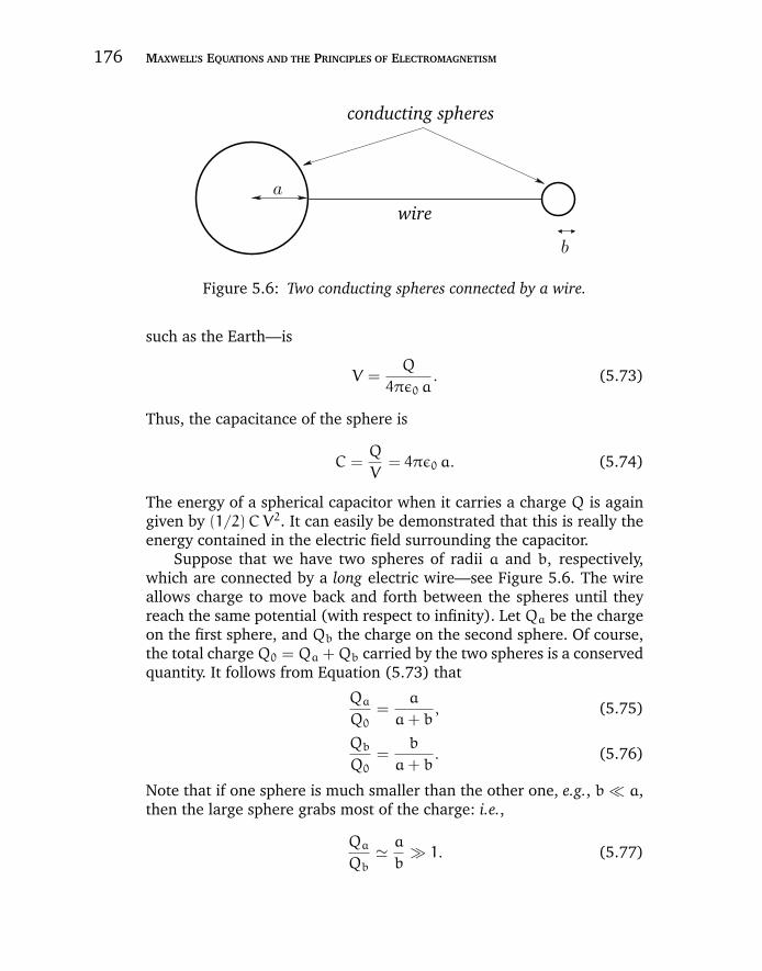
“chapter5” — 2007/11/29 — 15:40 — page 176 — #20
176 MAXWELL’S EQUATIONS AND THE PRINCIPLES OF ELECTROMAGNETISM
a
conducting spheres
wire
b
Figure 5.6: Two conducting spheres connected by a wire.
such as the Earth—is
V =Q
4πε0 a. (5.73)
Thus, the capacitance of the sphere is
C =Q
V= 4πε0 a. (5.74)
The energy of a spherical capacitor when it carries a charge Q is againgiven by (1/2)CV2. It can easily be demonstrated that this is really theenergy contained in the electric field surrounding the capacitor.
Suppose that we have two spheres of radii a and b, respectively,which are connected by a long electric wire—see Figure 5.6. The wireallows charge to move back and forth between the spheres until theyreach the same potential (with respect to infinity). Let Qa be the chargeon the first sphere, and Qb the charge on the second sphere. Of course,the total chargeQ0 = Qa +Qb carried by the two spheres is a conservedquantity. It follows from Equation (5.73) that
Qa
Q0=
a
a+ b, (5.75)
Qb
Q0=
b
a+ b. (5.76)
Note that if one sphere is much smaller than the other one, e.g., b a,then the large sphere grabs most of the charge: i.e.,
Qa
Qb a
b 1. (5.77)
“chapter5” — 2007/11/29 — 15:40 — page 177 — #21
CHAPTER 5 ELECTROSTATIC CALCULATIONS 177
The ratio of the electric fields generated just above the surfaces of thetwo spheres follows from Equations (5.72) and (5.77):
Eb
Ea a
b. (5.78)
Note that if b a then the field just above the smaller sphere is far largerthan that above the larger sphere. Equation (5.78) is a simple exampleof a far more general rule: i.e., the electric field above some point onthe surface of a conductor is inversely proportional to the local radius ofcurvature of the surface.
It is clear that if we wish to store significant amounts of charge ona conductor then the surface of the conductor must be made as smoothas possible. Any sharp spikes on the surface will inevitably have com-paratively small radii of curvature. Intense local electric fields are thusgenerated around such spikes. These fields can easily exceed the criti-cal field for the breakdown of air, leading to sparking and the eventualloss of the charge on the conductor. Sparking can also be very destruc-tive, because the associated electric currents flow through very localizedregions, giving rise to intense ohmic heating.
As a final example, consider two coaxial conducting cylinders of radiia and b, where a < b. Suppose that the charge per unit length carried bythe outer and inner cylinders is +λ and −λ, respectively. We can safelyassume that E = Er(r) er, by symmetry (adopting standard cylindricalpolar coordinates). Let us apply Gauss’ law to a cylindrical surface ofradius r, coaxial with the conductors, and of length l. For a < r < b, wefind that
2π r l Er(r) =λ l
ε0, (5.79)
so that
Er =λ
2πε0 r(5.80)
for a < r < b. It is fairly obvious that Er = 0 if r is not in the range a tob. The potential difference between the inner and outer cylinders is
V = −
∫ inner
outerE · dl =
∫outer
innerE · dl
=
∫ba
Er dr =λ
2πε0
∫ba
dr
r, (5.81)
“chapter5” — 2007/11/29 — 15:40 — page 178 — #22
178 MAXWELL’S EQUATIONS AND THE PRINCIPLES OF ELECTROMAGNETISM
so
V =λ
2πε0lnb
a. (5.82)
Thus, the capacitance per unit length of the two cylinders is
C =λ
V=2πε0
ln b/a. (5.83)
5.7 POISSON’S EQUATION
Now, we know that in a steady-state we can write
E = −∇φ, (5.84)
with the scalar potential satisfying Poisson’s equation:
∇2φ = −ρ
ε0. (5.85)
We even know the general solution to this equation:
φ(r) =1
4πε0
∫ρ(r ′)
|r − r ′|d3r ′. (5.86)
So, what else is there to say about Poisson’s equation? Well, considera positive (say) point charge in the vicinity of an uncharged, insulated,conducting sphere. The charge attracts negative charges to the near sideof the sphere, and repels positive charges to the far side. The surfacecharge distribution induced on the sphere is such that the surface ismaintained at a constant electrical potential. We now have a problem.We cannot use formula (5.86) to work out the potential φ(r) around thesphere, since we do not know beforehand how the charges induced onits conducting surface are distributed. The only things which we knowabout the surface are that it is an equipotential, and carries zero netcharge. Clearly, the solution (5.86) to Poisson’s equation is completelyuseless in the presence of conducting surfaces. Let us now try to developsome techniques for solving Poisson’s equation which allow us to solvereal problems (which invariably involve conductors).
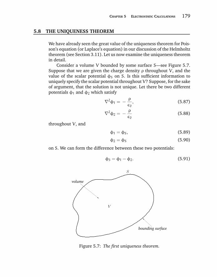
“chapter5” — 2007/11/29 — 15:40 — page 179 — #23
CHAPTER 5 ELECTROSTATIC CALCULATIONS 179
5.8 THE UNIQUENESS THEOREM
We have already seen the great value of the uniqueness theorem for Pois-son’s equation (or Laplace’s equation) in our discussion of the Helmholtztheorem (see Section 3.11). Let us now examine the uniqueness theoremin detail.
Consider a volume V bounded by some surface S—see Figure 5.7.Suppose that we are given the charge density ρ throughout V, and thevalue of the scalar potential φS on S. Is this sufficient information touniquely specify the scalar potential throughoutV? Suppose, for the sakeof argument, that the solution is not unique. Let there be two differentpotentials φ1 and φ2 which satisfy
∇2φ1 = −ρ
ε0, (5.87)
∇2φ2 = −ρ
ε0(5.88)
throughout V, and
φ1 = φS, (5.89)
φ2 = φS (5.90)
on S. We can form the difference between these two potentials:
φ3 = φ1 − φ2. (5.91)
V
S
bounding surface
volume
Figure 5.7: The first uniqueness theorem.
“chapter5” — 2007/11/29 — 15:40 — page 180 — #24
180 MAXWELL’S EQUATIONS AND THE PRINCIPLES OF ELECTROMAGNETISM
The potential φ3 clearly satisfies
∇2φ3 = 0 (5.92)
throughout V, and
φ3 = 0 (5.93)
on S.Now, according to vector field theory,
∇ · (φ3∇φ3) ≡ (∇φ3)2 + φ3∇2φ3. (5.94)
Thus, using Gauss’ theorem,∫V
[(∇φ3)2 + φ3∇2φ3
]dV =
∮S
φ3∇φ3 · dS. (5.95)
But, ∇2φ3 = 0 throughout V, and φ3 = 0 on S, so the above equationreduces to ∫
V
(∇φ3)2 dV = 0. (5.96)
Note that (∇φ3)2 is a positive definite quantity. The only way in whichthe volume integral of a positive definite quantity can be zero is if thatquantity itself is zero throughout the volume. This is not necessarily thecase for a non-positive definite quantity: we could have positive and neg-ative contributions from various regions inside the volume which cancelone another out. Thus, since (∇φ3)2 is positive definite, it follows that
φ3 = constant (5.97)
throughout V. However, we know that φ3 = 0 on S, so we get
φ3 = 0 (5.98)
throughout V. In other words,
φ1 = φ2 (5.99)
throughout V and on S. Our initial assumption that φ1 and φ2 are twodifferent solutions of Poisson’s equation, satisfying the same boundaryconditions, turns out to be incorrect. Hence, the solution is unique.
The fact that the solutions to Poisson’s equation are unique is veryuseful. It means that if we find a solution to this equation—no matter

“chapter5” — 2007/11/29 — 15:40 — page 181 — #25
CHAPTER 5 ELECTROSTATIC CALCULATIONS 181
S2 V
S
bounding surface
volume
S1
S3
conductors
Figure 5.8: The second uniqueness theorem.
how contrived the derivation—then this is the only possible solution.One immediate use of the uniqueness theorem is to prove that the electricfield inside an empty cavity situated within a conductor is zero. Recallthat our previous proof of this was rather involved, and was also notparticularly rigorous (see Section 5.4). Now, we know that the interiorsurface of the conductor is at some constant potential φ0, say. So, wehave φ = φ0 on the boundary of the cavity, and ∇2φ = 0 inside thecavity (since it contains no charges). One rather obvious solution to thisproblem is φ = φ0 throughout the cavity. Since the solutions to Poisson’sequation are unique, this is the only solution. Thus,
E = −∇φ = −∇φ0 = 0 (5.100)
inside the cavity.Suppose that some volume V contains a number of conductors—see
Figure 5.8. We know that the surface of each conductor is an equipoten-tial, but, in general, we do not know the potential of a given conductor(unless we are specifically told that the conductor is earthed, etc.). How-ever, if the conductors are insulated then it is plausible that we mightknow the charge on each conductor. Suppose that there are N conduc-tors, each carrying a known charge Qi (i = 1 to N), and suppose thatthe region V containing these conductors is filled by a known chargedensity ρ, and bounded by some surface S which is either infinity or anenclosing conductor. Is this sufficient information to uniquely specify theelectric field throughout V?
“chapter5” — 2007/11/29 — 15:40 — page 182 — #26
182 MAXWELL’S EQUATIONS AND THE PRINCIPLES OF ELECTROMAGNETISM
Well, suppose that it is not sufficient information, so that there aretwo different fields E1 and E2 which satisfy
∇ · E1 =ρ
ε0, (5.101)
∇ · E2 =ρ
ε0(5.102)
throughout V, with ∮Si
E1 · dSi =Qi
ε0, (5.103)
∮Si
E2 · dSi =Qi
ε0(5.104)
on the surface of the ith conductor, and, finally,∮S
E1 · dS =Qtotal
ε0, (5.105)
∮S
E2 · dS =Qtotal
ε0(5.106)
over the bounding surface, where
Qtotal =
N∑i=1
Qi +
∫V
ρdV (5.107)
is the total charge contained in volume V.Let us form the difference field
E3 = E1 − E2. (5.108)
It is clear that
∇ · E3 = 0 (5.109)
throughout V, and ∮Si
E3 · dSi = 0 (5.110)
for all i, with ∮S
E3 · dS = 0. (5.111)

“chapter5” — 2007/11/29 — 15:40 — page 183 — #27
CHAPTER 5 ELECTROSTATIC CALCULATIONS 183
Now, we know that each conductor is at a constant potential, so if
E3 = −∇φ3, (5.112)
then φ3 is a constant on the surface of each conductor. Furthermore,if the outer surface S is infinity then φ1 = φ2 = φ3 = 0 on this surface.On the other hand, if the outer surface is an enclosing conductor thenφ3 is a constant on it. Either way, φ3 is constant on S.
Consider the vector identity
∇ · (φ3 E3) ≡ φ3∇ · E3 + E3 · ∇φ3. (5.113)
We have ∇ · E3 = 0 throughout V, and ∇φ3 = −E3, so the above identityreduces to
∇ · (φ3 E3) = −E 23 (5.114)
throughout V. Integrating over V, and making use of Gauss’ theorem,yields
∫V
E 23 dV =
N∑i=1
∮Si
φ3 E3 · dSi −∮S
φ3 E3 · dS. (5.115)
However, φ3 is a constant on the surfaces Si and S. So, making use ofEquations (5.110) and (5.111), we obtain∫
V
E 23 dV = 0. (5.116)
Of course, E 23 is a positive definite quantity, so the above relation implies
that
E3 = 0 (5.117)
throughoutV: i.e., the fields E1 and E2 are identical throughoutV. Hence,the solution is unique.
For a general electrostatic problem involving charges and conduc-tors, it is clear that if we are given either the potential at the surface ofeach conductor or the charge carried by each conductor (plus the chargedensity throughout the volume, etc.) then we can uniquely determinethe electric field. There are many other uniqueness theorems which gen-eralize this result still further: e.g., we could be given the potentials onthe surfaces of some of the conductors, and the charges on the surfacesof the others, and the solution would still be unique.
“chapter5” — 2007/11/29 — 15:40 — page 184 — #28
184 MAXWELL’S EQUATIONS AND THE PRINCIPLES OF ELECTROMAGNETISM
At this point, it is worth noting that there are also uniqueness theo-rems associated with magnetostatics. For instance, if the current density,j, is specified throughout some volume V, and either the magnetic field,B, or the vector potential, A, is specified on the bounding surface S, thenthe magnetic field is uniquely determined throughout V and on S. Theproof of this proposition proceeds along the usual lines. Suppose thatthe magnetic field is not uniquely determined. In other words, supposethere are two different magnetic fields, B1 and B2, satisfying
∇ × B1 = µ0 j, (5.118)
∇ × B2 = µ0 j, (5.119)
throughout V. Suppose, further, that either B1 = B2 = BS or A1 = A2 =AS on S. Forming the difference field, B3 = B1 − B2, we have
∇ × B3 = 0 (5.120)
throughoutV, and either B3 = 0 or A3 = 0 on S. Now, according to vectorfield theory,∫
V
[(∇ × U)2 − U · ∇ × ∇ × U
]dV ≡
∮S
U × (∇ × U) · dS. (5.121)
Setting U = A3, and using B3 = ∇ × A3 and Equation (5.120), we obtain∫V
B23 dV =
∮S
A3 × B3 · dS. (5.122)
However, we know that either B3 or A3 is zero on S. Hence, we get∫V
B23 dV = 0. (5.123)
Since B23 is positive definite, the only way in which the above equationcan be satisfied is if B3 is zero throughout V. Hence, B1 = B2 throughoutV, and the solution is unique.
5.9 ONE-DIMENSIONAL SOLUTIONS OF POISSON’S EQUATION
So, how do we actually solve Poisson’s equation,
∂2φ
∂x2+∂2φ
∂y2+∂2φ
∂z2= −
ρ(x, y, z)
ε0, (5.124)
“chapter5” — 2007/11/29 — 15:40 — page 185 — #29
CHAPTER 5 ELECTROSTATIC CALCULATIONS 185
in practice? In general, the answer is that we use a computer. However,there are a few situations, possessing a high degree of symmetry, whereit is possible to find analytic solutions. Let us discuss some of thesesituations.
Suppose, first of all, that there is no variation of quantities in (say)the y- and z-directions. In this case, Poisson’s equation reduces to anordinary differential equation in x, the solution of which is relativelystraightforward. Consider, for instance, a vacuum diode, in which elec-trons are emitted from a hot cathode and accelerated toward an anode,which is held at a large positive potential V with respect to the cathode.We can think of this as an essentially one-dimensional problem. Supposethat the cathode is at x = 0 and the anode at x = d. Poisson’s equationtakes the form
d2φ
dx2= −
ρ(x)
ε0, (5.125)
whereφ(x) satisfies the boundary conditionsφ(0) = 0 andφ(d) = V. Byenergy conservation, an electron emitted from rest at the cathode hasan x-velocity v(x) which satisfies
1
2me v
2(x) − eφ(x) = 0. (5.126)
Here, me and −e are the mass and charge of an electron, respectively.Finally, in a steady-state, the electric current I (between the anode andcathode) is independent of x (otherwise, charge will continually buildup at some points). In fact,
I = −ρ(x) v(x)A, (5.127)
where A is the cross-sectional area of the diode. The previous threeequations can be combined to give
d2φ
dx2=
I
ε0 A
(me
2 e
)1/2φ−1/2. (5.128)
The solution of the above equation which satisfies the boundary condi-tions is
φ(x) = V(xd
)4/3, (5.129)
with
I =4
9
ε0 A
d2
(2 e
me
)1/2V3/2. (5.130)
“chapter5” — 2007/11/29 — 15:40 — page 186 — #30
186 MAXWELL’S EQUATIONS AND THE PRINCIPLES OF ELECTROMAGNETISM
This relationship between the current and the voltage in a vacuum diodeis called the Child-Langmuir law.
Let us now consider the solution of Poisson’s equation in more thanone dimension.
5.10 THE METHOD OF IMAGES
Suppose that we have a point charge q held a distance d from an infi-nite, grounded, conducting plate—see Figure 5.9. Let the plate lie in thex-y plane, and suppose that the point charge is located at coordinates(0, 0, d). What is the scalar potential generated in the region above theplate? This is not a simple question, because the point charge inducessurface charges on the plate, and we do not know beforehand how thesecharges are distributed.
Well, what do we know in this problem? We know that the conduct-ing plate is an equipotential surface. In fact, the potential of the plate iszero, since it is grounded. We also know that the potential at infinity iszero (this is our usual boundary condition for the scalar potential). Thus,we need to solve Poisson’s equation in the region z > 0, with a singlepoint charge q at position (0, 0, d), subject to the boundary conditions
φ(x, y, 0) = 0, (5.131)
and
φ(x, y, z) → 0 as x2 + y2 + z2 → ∞. (5.132)
Let us forget about the real problem, for a moment, and concentrateon a slightly different one. We refer to this as the analog problem—seeFigure 5.9. In the analog problem, we have a charge q located at (0, 0, d)and a charge −q located at (0, 0, -d), with no conductors present. Wecan easily find the scalar potential for this problem, since we know whereall the charges are located. We get
φanalog(x, y, z) =1
4πε0
q√
x2 + y2 + (z− d)2−
q√x2 + y2 + (z+ d)2
.
(5.133)
Note, however, thatφanalog(x, y, 0) = 0, (5.134)
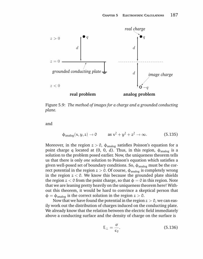
“chapter5” — 2007/11/29 — 15:40 — page 187 — #31
CHAPTER 5 ELECTROSTATIC CALCULATIONS 187
analog problem
d
d
d
z = 0
−q
image charge
real problem
real charge
grounded conducting plate
z > 0
z < 0
Figure 5.9: The method of images for a charge and a grounded conductingplane.
and
φanalog(x, y, z) → 0 as x2 + y2 + z2 → ∞. (5.135)
Moreover, in the region z > 0, φanalog satisfies Poisson’s equation for apoint charge q located at (0, 0, d). Thus, in this region, φanalog is asolution to the problem posed earlier. Now, the uniqueness theorem tellsus that there is only one solution to Poisson’s equation which satisfies agiven well-posed set of boundary conditions. So, φanalog must be the cor-rect potential in the region z > 0. Of course, φanalog is completely wrongin the region z < 0. We know this because the grounded plate shieldsthe region z < 0 from the point charge, so that φ = 0 in this region. Notethat we are leaning pretty heavily on the uniqueness theorem here! With-out this theorem, it would be hard to convince a skeptical person thatφ = φanalog is the correct solution in the region z > 0.
Now that we have found the potential in the region z > 0, we can eas-ily work out the distribution of charges induced on the conducting plate.We already know that the relation between the electric field immediatelyabove a conducting surface and the density of charge on the surface is
E⊥ =σ
ε0. (5.136)
“chapter5” — 2007/11/29 — 15:40 — page 188 — #32
188 MAXWELL’S EQUATIONS AND THE PRINCIPLES OF ELECTROMAGNETISM
In this case,
E⊥(x, y) = Ez(x, y, 0+) = −∂φ(x, y, 0+)
∂z= −
∂φanalog(x, y, 0+)
∂z,
(5.137)so
σ(x, y) = −ε0∂φanalog(x, y, 0+)
∂z. (5.138)
Now, it follows from Equation (5.133) that
∂φanalog
∂z=
q
4πε0
−(z− d)
[x2 + y2 + (z− d)2]3/2+
(z+ d)
[x2 + y2 + (z+ d)2]3/2
,
(5.139)
so
σ(x, y) = −qd
2π (x2 + y2 + d2)3/2. (5.140)
Clearly, the charge induced on the plate has the opposite sign to thepoint charge. The charge density on the plate is also symmetric aboutthe z-axis, and is largest where the plate is closest to the point charge.The total charge induced on the plate is
Q =
∫x−y plane
σdS, (5.141)
which yields
Q = −qd
2π
∫∞
0
2π r dr
(r2 + d2)3/2, (5.142)
where r2 = x2 + y2. Thus,
Q = −qd
2
∫∞
0
dk
(k+ d2)3/2= qd
[1
(k+ d2)1/2
]∞
0
= −q. (5.143)
So, the total charge induced on the plate is equal and opposite to thepoint charge which induces it.
As we have just seen, our point charge induces charges of the oppo-site sign on the conducting plate. This, presumably, gives rise to a forceof attraction between the charge and the plate. What is this force? Well,since the potentials, and, hence, the electric fields, in the vicinity of the
“chapter5” — 2007/11/29 — 15:40 — page 189 — #33
CHAPTER 5 ELECTROSTATIC CALCULATIONS 189
point charge are the same in the real and analog problems, the forceson this charge must be the same as well. In the analog problem, thereare two charges ±q a net distance 2 d apart. The force on the charge atposition (0, 0, d) (i.e., the real charge) is
f = −q2
16πε0 d2ez. (5.144)
Hence, this is also the force on the charge in the real problem.What, finally, is the potential energy of the system. For the analog
problem this is simply
Wanalog = −q2
8πε0 d. (5.145)
Note that in the analog problem the fields on opposite sides of the con-ducting plate are mirror images of one another. So are the charges (apartfrom the change in sign). This is why the technique of replacing con-ducting surfaces by imaginary charges is called the method of images.We know that the potential energy of a set of charges is equivalent tothe energy stored in the electric field. Thus,
W =ε0
2
∫all space
E2 dV. (5.146)
Moreover, as we just mentioned, in the analog problem, the fields oneither side of the x-y plane are mirror images of one another, so thatE2(x, y,−z) = E2(x, y, z). It follows that
Wanalog = 2ε0
2
∫z>0
E2analog dV. (5.147)
Now, in the real problem
E =
Eanalog for z > 00 for z < 0
. (5.148)
So,
W =ε0
2
∫z>0
E2 dV =ε0
2
∫z>0
E2analog dV =1
2Wanalog, (5.149)
giving
W = −q2
16πε0 d. (5.150)
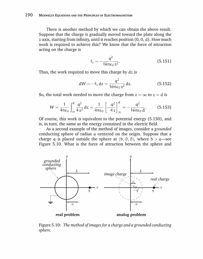
“chapter5” — 2007/11/29 — 15:40 — page 190 — #34
190 MAXWELL’S EQUATIONS AND THE PRINCIPLES OF ELECTROMAGNETISM
There is another method by which we can obtain the above result.Suppose that the charge is gradually moved toward the plate along thez-axis, starting from infinity, until it reaches position (0, 0, d). How muchwork is required to achieve this? We know that the force of attractionacting on the charge is
fz = −q2
16πε0 z2. (5.151)
Thus, the work required to move this charge by dz is
dW = −fz dz =q2
16πε0 z2dz. (5.152)
So, the total work needed to move the charge from z = ∞ to z = d is
W =1
4πε0
∫d∞
q2
4 z2dz =
1
4πε0
[−q2
4 z
]d∞
= −q2
16πε0 d. (5.153)
Of course, this work is equivalent to the potential energy (5.150), andis, in turn, the same as the energy contained in the electric field.
As a second example of the method of images, consider a groundedconducting sphere of radius a centered on the origin. Suppose that acharge q is placed outside the sphere at (b, 0, 0), where b > a—seeFigure 5.10. What is the force of attraction between the sphere and
analog problem
conductingsphere
real problem
a
b b
x x
y y
q q−q′
creal charge
image charge
a
grounded
Figure 5.10: The method of images for a charge and a grounded conductingsphere.
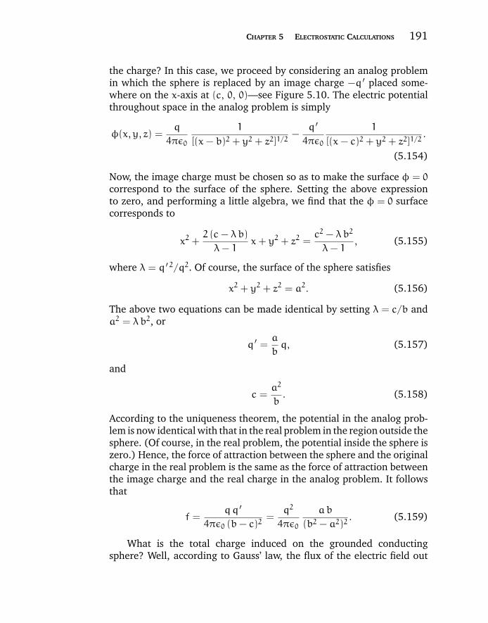
“chapter5” — 2007/11/29 — 15:40 — page 191 — #35
CHAPTER 5 ELECTROSTATIC CALCULATIONS 191
the charge? In this case, we proceed by considering an analog problemin which the sphere is replaced by an image charge −q ′ placed some-where on the x-axis at (c, 0, 0)—see Figure 5.10. The electric potentialthroughout space in the analog problem is simply
φ(x, y, z) =q
4πε0
1
[(x− b)2 + y2 + z2]1/2−
q ′
4πε0
1
[(x− c)2 + y2 + z2]1/2.
(5.154)
Now, the image charge must be chosen so as to make the surface φ = 0
correspond to the surface of the sphere. Setting the above expressionto zero, and performing a little algebra, we find that the φ = 0 surfacecorresponds to
x2 +2 (c− λb)
λ− 1x+ y2 + z2 =
c2 − λb2
λ− 1, (5.155)
where λ = q ′ 2/q2. Of course, the surface of the sphere satisfies
x2 + y2 + z2 = a2. (5.156)
The above two equations can be made identical by setting λ = c/b anda2 = λb2, or
q ′ =a
bq, (5.157)
and
c =a2
b. (5.158)
According to the uniqueness theorem, the potential in the analog prob-lem is now identical with that in the real problem in the region outside thesphere. (Of course, in the real problem, the potential inside the sphere iszero.) Hence, the force of attraction between the sphere and the originalcharge in the real problem is the same as the force of attraction betweenthe image charge and the real charge in the analog problem. It followsthat
f =qq ′
4πε0 (b− c)2=
q2
4πε0
ab
(b2 − a2)2. (5.159)
What is the total charge induced on the grounded conductingsphere? Well, according to Gauss’ law, the flux of the electric field out
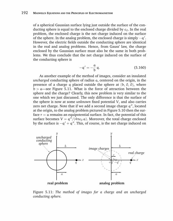
“chapter5” — 2007/11/29 — 15:40 — page 192 — #36
192 MAXWELL’S EQUATIONS AND THE PRINCIPLES OF ELECTROMAGNETISM
of a spherical Gaussian surface lying just outside the surface of the con-ducting sphere is equal to the enclosed charge divided by ε0. In the realproblem, the enclosed charge is the net charge induced on the surfaceof the sphere. In the analog problem, the enclosed charge is simply −q ′.However, the electric fields outside the conducting sphere are identicalin the real and analog problems. Hence, from Gauss’ law, the chargeenclosed by the Gaussian surface must also be the same in both prob-lems. We thus conclude that the net charge induced on the surface ofthe conducting sphere is
−q ′ = −a
bq. (5.160)
As another example of the method of images, consider an insulateduncharged conducting sphere of radius a, centered on the origin, in thepresence of a charge q placed outside the sphere at (b, 0, 0), whereb > a—see Figure 5.11. What is the force of attraction between thesphere and the charge? Clearly, this new problem is very similar to theone which we just discussed. The only difference is that the surface ofthe sphere is now at some unknown fixed potential V, and also carrieszero net charge. Note that if we add a second image charge q ′′, locatedat the origin, to the analog problem pictured in Figure 5.10 then the sur-face r = a remains an equipotential surface. In fact, the potential of thissurface becomes V = q ′′/(4πε0 a). Moreover, the total charge enclosedby the surface is −q ′ + q ′′. This, of course, is the net charge induced on
−q′
conductingsphere
real problem
a
b b
x x
y y
q q
creal charge
a
analog problem
uncharged
image charges
+q′
Figure 5.11: The method of images for a charge and an unchargedconducting sphere.
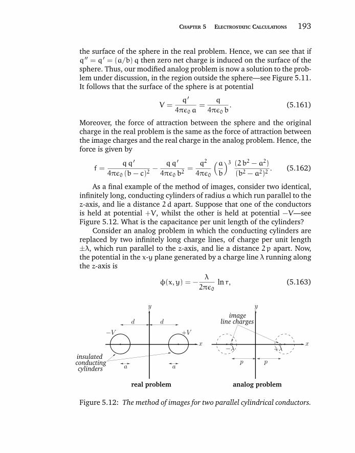
“chapter5” — 2007/11/29 — 15:40 — page 193 — #37
CHAPTER 5 ELECTROSTATIC CALCULATIONS 193
the surface of the sphere in the real problem. Hence, we can see that ifq ′′ = q ′ = (a/b)q then zero net charge is induced on the surface of thesphere. Thus, our modified analog problem is now a solution to the prob-lem under discussion, in the region outside the sphere—see Figure 5.11.It follows that the surface of the sphere is at potential
V =q ′
4πε0 a=
q
4πε0 b. (5.161)
Moreover, the force of attraction between the sphere and the originalcharge in the real problem is the same as the force of attraction betweenthe image charges and the real charge in the analog problem. Hence, theforce is given by
f =qq ′
4πε0 (b− c)2−
qq ′
4πε0 b2=
q2
4πε0
(ab
)3 (2 b2 − a2)
(b2 − a2)2. (5.162)
As a final example of the method of images, consider two identical,infinitely long, conducting cylinders of radius awhich run parallel to thez-axis, and lie a distance 2 d apart. Suppose that one of the conductorsis held at potential +V, whilst the other is held at potential −V—seeFigure 5.12. What is the capacitance per unit length of the cylinders?
Consider an analog problem in which the conducting cylinders arereplaced by two infinitely long charge lines, of charge per unit length±λ, which run parallel to the z-axis, and lie a distance 2 p apart. Now,the potential in the x-y plane generated by a charge line λ running alongthe z-axis is
φ(x, y) = −λ
2πε0ln r, (5.163)
y
x x
insulatedconductingcylinders
imageline chargesd d
a ap p
−V
−λ +λ
+V
real problem analog problem
y
Figure 5.12: The method of images for two parallel cylindrical conductors.
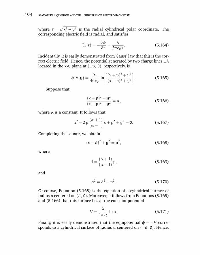
“chapter5” — 2007/11/29 — 15:40 — page 194 — #38
194 MAXWELL’S EQUATIONS AND THE PRINCIPLES OF ELECTROMAGNETISM
where r =√x2 + y2 is the radial cylindrical polar coordinate. The
corresponding electric field is radial, and satisfies
Er(r) = −∂φ
∂r=
λ
2πε0 r. (5.164)
Incidentally, it is easily demonstrated from Gauss’ law that this is the cor-rect electric field. Hence, the potential generated by two charge lines ±λlocated in the x-y plane at (±p, 0), respectively, is
φ(x, y) =λ
4πε0ln[(x+ p)2 + y2
(x− p)2 + y2
]. (5.165)
Suppose that
(x+ p)2 + y2
(x− p)2 + y2= α, (5.166)
where α is a constant. It follows that
x2 − 2 p(α+ 1)
(α− 1)x+ p2 + y2 = 0. (5.167)
Completing the square, we obtain
(x− d)2 + y2 = a2, (5.168)
where
d =(α+ 1)
(α− 1)p, (5.169)
and
a2 = d2 − p2. (5.170)
Of course, Equation (5.168) is the equation of a cylindrical surface ofradius a centered on (d, 0). Moreover, it follows from Equations (5.165)and (5.166) that this surface lies at the constant potential
V =λ
4πε0lnα. (5.171)
Finally, it is easily demonstrated that the equipotential φ = −V corre-sponds to a cylindrical surface of radius a centered on (−d, 0). Hence,
“chapter5” — 2007/11/29 — 15:40 — page 195 — #39
CHAPTER 5 ELECTROSTATIC CALCULATIONS 195
we can make the analog problem match the real problem in the regionoutside the cylinders by choosing
α =d+ p
d− p=d+
√d2 − a2
d−√d2 − a2
. (5.172)
Thus, we obtain
V =λ
4πε0ln
(d+
√d2 − a2
d−√d2 − a2
). (5.173)
Now, it follows from Gauss’ law, and the fact that the electric fields inthe real and analog problems are identical outside the cylinders, that thecharge per unit length stored on the surfaces of the two cylinders is ±λ.Moreover, the voltage difference between the cylinders is 2V. Hence,the capacitance per unit length of the cylinders is C = λ/(2V), yielding
C = 2πε0
/ln
(d+
√d2 − a2
d−√d2 − a2
). (5.174)
This expression simplifies to give
C = πε0
/ln
(d
a+
√d2
a2− 1
), (5.175)
which can also be written
C =πε0
cosh−1(d/a), (5.176)
since cosh−1 x ≡ ln(x+√x2 − 1).
5.11 COMPLEX ANALYSIS
Let us now investigate another trick for solving Poisson’s equation (actu-ally it only solves Laplace’s equation). Unfortunately, this method onlyworks in two dimensions.
The complex variable is conventionally written
z = x+ iy, (5.177)
where x and y are both real, and are identified with the correspondingCartesian coordinates. (Incidentally, z should not be confused with a
“chapter5” — 2007/11/29 — 15:40 — page 196 — #40
196 MAXWELL’S EQUATIONS AND THE PRINCIPLES OF ELECTROMAGNETISM
z-coordinate: this is a strictly two-dimensional discussion.) We can writefunctions F(z) of the complex variable just like we would write functionsof a real variable. For instance,
F(z) = z2, (5.178)
F(z) =1
z. (5.179)
For a given function, F(z), we can substitute z = x+ iy and write
F(z) = U(x, y) + iV(x, y), (5.180)
where U and V are two real two-dimensional functions. Thus, if
F(z) = z2, (5.181)
then
F(x+ iy) = (x+ iy)2 = (x2 − y2) + 2 i xy, (5.182)
giving
U(x, y) = x2 − y2, (5.183)
V(x, y) = 2 x y. (5.184)
We can define the derivative of a complex function in just the samemanner as we would define the derivative of a real function: i.e.,
dF
dz= lim |δz|→∞
F(z+ δz) − F(z)
δz. (5.185)
However, we now have a slight problem. If F(z) is a “well-defined”function (we shall leave it to the mathematicians to specify exactly whatbeing well-defined entails: suffice to say that most functions we canthink of are well-defined) then it should not matter from which directionin the complex plane we approach z when taking the limit in Equa-tion (5.185). There are, of course, many different directions we couldapproach z from, but if we look at a regular complex function, F(z) = z2
(say), then
dF
dz= 2 z (5.186)
is perfectly well-defined, and is, therefore, completely independent ofthe details of how the limit is taken in Equation (5.185).
“chapter5” — 2007/11/29 — 15:40 — page 197 — #41
CHAPTER 5 ELECTROSTATIC CALCULATIONS 197
The fact that Equation (5.185) has to give the same result, no matterfrom which direction we approach z, means that there are some restric-tions on the forms of the functionsU and V in Equation (5.180). Supposethat we approach z along the real axis, so that δz = δx. We obtain
dF
dz= lim |δx|→0
U(x+ δx, y) + iV(x+ δx, y) −U(x, y) − iV(x, y)
δx
=∂U
∂x+ i
∂V
∂x. (5.187)
Suppose that we now approach z along the imaginary axis, so that δz =i δy. We get
dF
dz= lim |δy|→0
U(x, y+ δy) + iV(x, y+ δy) −U(x, y) − iV(x, y)
i δy
= − i∂U
∂y+∂V
∂y. (5.188)
But, if F(z) is a well-defined function then its derivative must also be well-defined, which implies that the above two expressions are equivalent.This requires that
∂U
∂x=∂V
∂y, (5.189)
∂V
∂x= −
∂U
∂y. (5.190)
These are called the Cauchy-Riemann relations, and are, in fact, sufficientto ensure that all possible ways of taking the limit (5.185) give the sameanswer.
So far, we have found that a general complex function F(z) can bewritten
F(z) = U(x, y) + iV(x, y), (5.191)
where z = x+ iy. If F(z) is well-defined then U and V automaticallysatisfy the Cauchy-Riemann relations. But, what has all of this got todo with electrostatics? Well, we can combine the two Cauchy-Riemannrelations to give
∂2U
∂x2=∂
∂x
∂V
∂y=∂
∂y
∂V
∂x= −
∂
∂y
∂U
∂y, (5.192)
“chapter5” — 2007/11/29 — 15:40 — page 198 — #42
198 MAXWELL’S EQUATIONS AND THE PRINCIPLES OF ELECTROMAGNETISM
and
∂2V
∂x2= −
∂
∂x
∂U
∂y= −
∂
∂y
∂U
∂x= −
∂
∂y
∂V
∂y, (5.193)
which reduce to
∂2U
∂x2+∂2U
∂y2= 0, (5.194)
∂2V
∂x2+∂2V
∂y2= 0. (5.195)
Thus, both U and V automatically satisfy Laplace’s equation in twodimensions: i.e., both U and V are possible two-dimensional scalarpotentials in free space.
Consider the two-dimensional gradients of U and V:
∇U =
(∂U
∂x,∂U
∂y
), (5.196)
∇V =
(∂V
∂x,∂V
∂y
). (5.197)
Now
∇U · ∇V =∂U
∂x
∂V
∂x+∂U
∂y
∂V
∂y. (5.198)
However, it follows from the Cauchy-Riemann relations that
∇U · ∇V =∂V
∂y
∂V
∂x−∂V
∂x
∂V
∂y= 0. (5.199)
Thus, the contours of U are everywhere perpendicular to the contours ofV. It follows that if U maps out the contours of some free-space scalarpotential then the contours of V indicate the directions of the associatedelectric field-lines, and vice versa.
For every well-defined complex function, we get two sets of free-space potentials, and the associated electric field-lines. For example,consider the function F(z) = z2, for which
U(x, y) = x2 − y2, (5.200)
V(x, y) = 2 x y. (5.201)
These are, in fact, the equations of two sets of orthogonal hyperboloids—see Figure 5.13. So, U(x, y) (the solid lines in Figure 5.13) might
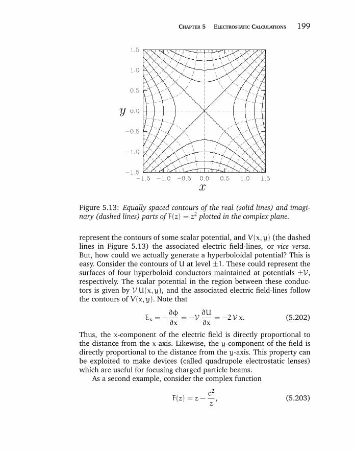
“chapter5” — 2007/11/29 — 15:40 — page 199 — #43
CHAPTER 5 ELECTROSTATIC CALCULATIONS 199
x
y
Figure 5.13: Equally spaced contours of the real (solid lines) and imagi-nary (dashed lines) parts of F(z) = z2 plotted in the complex plane.
represent the contours of some scalar potential, and V(x, y) (the dashedlines in Figure 5.13) the associated electric field-lines, or vice versa.But, how could we actually generate a hyperboloidal potential? This iseasy. Consider the contours of U at level ±1. These could represent thesurfaces of four hyperboloid conductors maintained at potentials ±V,respectively. The scalar potential in the region between these conduc-tors is given by V U(x, y), and the associated electric field-lines followthe contours of V(x, y). Note that
Ex = −∂φ
∂x= −V ∂U
∂x= −2V x. (5.202)
Thus, the x-component of the electric field is directly proportional tothe distance from the x-axis. Likewise, the y-component of the field isdirectly proportional to the distance from the y-axis. This property canbe exploited to make devices (called quadrupole electrostatic lenses)which are useful for focusing charged particle beams.
As a second example, consider the complex function
F(z) = z−c2
z, (5.203)
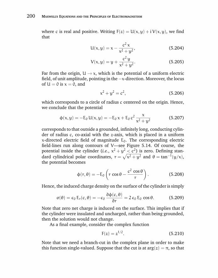
“chapter5” — 2007/11/29 — 15:40 — page 200 — #44
200 MAXWELL’S EQUATIONS AND THE PRINCIPLES OF ELECTROMAGNETISM
where c is real and positive. Writing F(z) = U(x, y) + iV(x, y), we findthat
U(x, y) = x−c2 x
x2 + y2, (5.204)
V(x, y) = y+c2 y
x2 + y2. (5.205)
Far from the origin, U → x, which is the potential of a uniform electricfield, of unit amplitude, pointing in the −x-direction. Moreover, the locusof U = 0 is x = 0, and
x2 + y2 = c2, (5.206)
which corresponds to a circle of radius c centered on the origin. Hence,we conclude that the potential
φ(x, y) = −E0 U(x, y) = −E0 x+ E0 c2 x
x2 + y2(5.207)
corresponds to that outside a grounded, infinitely long, conducting cylin-der of radius c, co-axial with the z-axis, which is placed in a uniformx-directed electric field of magnitude E0. The corresponding electricfield-lines run along contours of V—see Figure 5.14. Of course, thepotential inside the cylinder (i.e., x2 + y2 < c2) is zero. Defining stan-dard cylindrical polar coordinates, r =
√x2 + y2 and θ = tan−1(y/x),
the potential becomes
φ(r, θ) = −E0
(r cos θ−
c2 cos θr
). (5.208)
Hence, the induced charge density on the surface of the cylinder is simply
σ(θ) = ε0 Er(c, θ) = −ε0∂φ(c, θ)
∂r= 2 ε0 E0 cos θ. (5.209)
Note that zero net charge is induced on the surface. This implies that ifthe cylinder were insulated and uncharged, rather than being grounded,then the solution would not change.
As a final example, consider the complex function
F(z) = z1/2. (5.210)
Note that we need a branch-cut in the complex plane in order to makethis function single-valued. Suppose that the cut is at arg(z) = π, so that
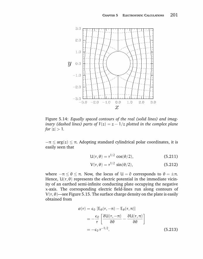
“chapter5” — 2007/11/29 — 15:40 — page 201 — #45
CHAPTER 5 ELECTROSTATIC CALCULATIONS 201
x
y
Figure 5.14: Equally spaced contours of the real (solid lines) and imag-inary (dashed lines) parts of F(z) = z− 1/z plotted in the complex planefor |z| > 1.
−π ≤ arg(z) ≤ π. Adopting standard cylindrical polar coordinates, it iseasily seen that
U(r, θ) = r1/2 cos(θ/2), (5.211)
V(r, θ) = r1/2 sin(θ/2), (5.212)
where −π ≤ θ ≤ π. Now, the locus of U = 0 corresponds to θ = ±π.Hence, U(r, θ) represents the electric potential in the immediate vicin-ity of an earthed semi-infinite conducting plate occupying the negativex-axis. The corresponding electric field-lines run along contours ofV(r, θ)—see Figure 5.15. The surface charge density on the plate is easilyobtained from
σ(r) = ε0 [Eθ(r,−π) − Eθ(r, π)]
= −ε0
r
[∂U(r,−π)
∂θ−∂U(r, π)
∂θ
]
= −ε0 r−1/2. (5.213)
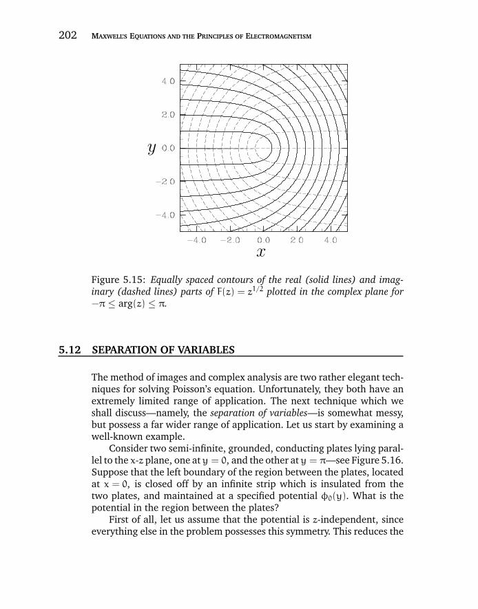
“chapter5” — 2007/11/29 — 15:40 — page 202 — #46
202 MAXWELL’S EQUATIONS AND THE PRINCIPLES OF ELECTROMAGNETISM
x
y
Figure 5.15: Equally spaced contours of the real (solid lines) and imag-inary (dashed lines) parts of F(z) = z1/2 plotted in the complex plane for−π ≤ arg(z) ≤ π.
5.12 SEPARATION OF VARIABLES
The method of images and complex analysis are two rather elegant tech-niques for solving Poisson’s equation. Unfortunately, they both have anextremely limited range of application. The next technique which weshall discuss—namely, the separation of variables—is somewhat messy,but possess a far wider range of application. Let us start by examining awell-known example.
Consider two semi-infinite, grounded, conducting plates lying paral-lel to the x-z plane, one at y = 0, and the other at y = π—see Figure 5.16.Suppose that the left boundary of the region between the plates, locatedat x = 0, is closed off by an infinite strip which is insulated from thetwo plates, and maintained at a specified potential φ0(y). What is thepotential in the region between the plates?
First of all, let us assume that the potential is z-independent, sinceeverything else in the problem possesses this symmetry. This reduces the
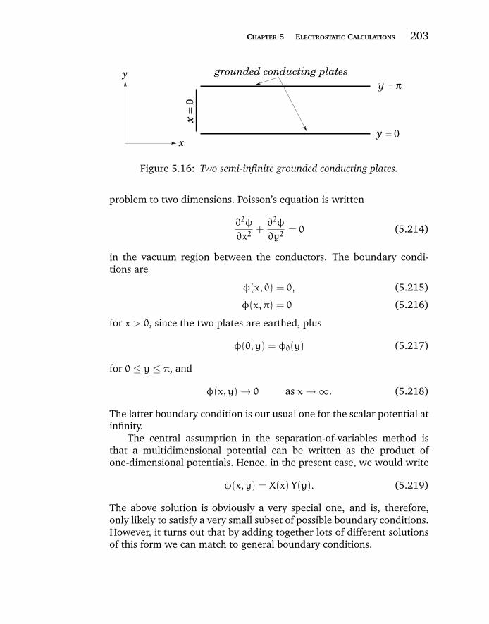
“chapter5” — 2007/11/29 — 15:40 — page 203 — #47
CHAPTER 5 ELECTROSTATIC CALCULATIONS 203
grounded conducting platesy = π
x =
0
y = 0
y
x
Figure 5.16: Two semi-infinite grounded conducting plates.
problem to two dimensions. Poisson’s equation is written
∂2φ
∂x2+∂2φ
∂y2= 0 (5.214)
in the vacuum region between the conductors. The boundary condi-tions are
φ(x, 0) = 0, (5.215)
φ(x, π) = 0 (5.216)
for x > 0, since the two plates are earthed, plus
φ(0, y) = φ0(y) (5.217)
for 0 ≤ y ≤ π, and
φ(x, y) → 0 as x → ∞. (5.218)
The latter boundary condition is our usual one for the scalar potential atinfinity.
The central assumption in the separation-of-variables method isthat a multidimensional potential can be written as the product ofone-dimensional potentials. Hence, in the present case, we would write
φ(x, y) = X(x)Y(y). (5.219)
The above solution is obviously a very special one, and is, therefore,only likely to satisfy a very small subset of possible boundary conditions.However, it turns out that by adding together lots of different solutionsof this form we can match to general boundary conditions.
“chapter5” — 2007/11/29 — 15:40 — page 204 — #48
204 MAXWELL’S EQUATIONS AND THE PRINCIPLES OF ELECTROMAGNETISM
Substituting (5.219) into (5.214), we obtain
Yd2X
dx2+ X
d2Y
dy2= 0. (5.220)
Let us now separate the variables: i.e., let us collect all of the x-dependentterms on one side of the equation, and all of the y-dependent terms onthe other side. Hence,
1
X
d2X
dx2= −
1
Y
d2Y
dy2. (5.221)
This equation has the form
f(x) = g(y), (5.222)
where f and g are general functions. The only way in which the aboveequation can be satisfied, for general x and y, is if both sides are equalto the same constant. Thus,
1
X
d2X
dx2= k2 = −
1
Y
d2Y
dy2. (5.223)
The reason why we write k2, rather than −k2, will become apparent lateron. Equation (5.223) separates into two ordinary differential equations:
d2X
dx2= k2 X, (5.224)
d2Y
dy2= −k2 Y. (5.225)
We know the general solution to these equations:
X = A exp(k x) + B exp(−k x), (5.226)
Y = C sin(ky) +D cos(ky), (5.227)
giving
φ(x, y) = [A exp(k x) + B exp(−k x) ] [C sin(ky) +D cos(ky)].(5.228)
Here, A, B, C, and D are arbitrary constants. The boundary condition(5.218) is automatically satisfied ifA = 0 and k > 0. Note that the choicek2, instead of −k2, in Equation (5.223) facilitates this by makingφ either
“chapter5” — 2007/11/29 — 15:40 — page 205 — #49
CHAPTER 5 ELECTROSTATIC CALCULATIONS 205
grow or decay monotonically in the x-direction instead of oscillating.The boundary condition (5.215) is automatically satisfied if D = 0. Theboundary condition (5.216) is satisfied provided that
sin(kπ) = 0, (5.229)
which implies that k is a positive integer, n (say). So, our solutionreduces to
φ(x, y) = C exp(−nx) sin(ny), (5.230)
where B has been absorbed into C. Note that this solution is only ableto satisfy the final boundary condition (5.217) provided that φ0(y) isproportional to sin(ny). Thus, at first sight, it would appear that themethod of separation of variables only works for a very special subset ofboundary conditions. However, this is not the case.
Now comes the clever bit! Since Poisson’s equation is linear, anylinear combination of solutions is also a solution. We can therefore forma more general solution than (5.230) by adding together lots of solutionsinvolving different values of n. Thus,
φ(x, y) =
∞∑n=1
Cn exp(−nx) sin(ny), (5.231)
where the Cn are constants. This solution automatically satisfies theboundary conditions (5.215), (5.216), and (5.218). The final boundarycondition (5.217) reduces to
φ(0, y) =
∞∑n=1
Cn sin(ny) = φ0(y). (5.232)
But, what choice of theCn fits an arbitrary functionφ0(y)? To answerthis question, we can make use of two very useful properties of thefunctions sin(ny). Namely, that they are mutually orthogonal, and forma complete set. The orthogonality property of these functions manifestsitself through the relation∫π
0
sin(ny) sin(n ′ y) dy =π
2δnn ′ , (5.233)
where δnn ′—which is equal to 1 if n = n ′, and 0, otherwise—is calleda Kroenecker delta function. The completeness property of sine func-tions means that any general function φ0(y) can always be adequately
“chapter5” — 2007/11/29 — 15:40 — page 206 — #50
206 MAXWELL’S EQUATIONS AND THE PRINCIPLES OF ELECTROMAGNETISM
represented as a weighted sum of sine functions with various differentn values. Multiplying both sides of Equation (5.232) by sin(n ′ y), andintegrating over y, we obtain
∞∑n=1
Cn
∫π0
sin(ny) sin(n ′ y) dy =
∫π0
φ0(y) sin(n ′ y) dy. (5.234)
The orthogonality relation yields
π
2
∞∑n=1
Cn δnn ′ =π
2Cn ′ =
∫π0
φ0(y) sin(n ′ y) dy, (5.235)
so
Cn =2
π
∫π0
φ0(y) sin(ny)dy. (5.236)
Thus, we now have a general solution to the problem for any drivingpotential φ0(y).
If the potential φ0(y) is constant then
Cn =2φ0
π
∫π0
sin(ny) dy =2φ0
nπ[1− cos(nπ)], (5.237)
giving
Cn = 0 (5.238)
for even n, and
Cn =4φ0
nπ(5.239)
for odd n. Thus,
φ(x, y) =4φ0
π
∑n=1,3,5,···
exp(−nx) sin(ny)
n. (5.240)
This potential is plotted in Figure 5.17.In the above problem, we wrote the potential as the product of
one-dimensional functions. Some of these functions grew and decayedmonotonically (i.e., the exponential functions), and the others oscillated(i.e., the sinusoidal functions). The success of the separation-of-variablesmethod depends crucially on the orthogonality and completeness of the
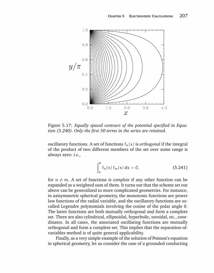
“chapter5” — 2007/11/29 — 15:40 — page 207 — #51
CHAPTER 5 ELECTROSTATIC CALCULATIONS 207
x
y/π
Figure 5.17: Equally spaced contours of the potential specified in Equa-tion (5.240). Only the first 50 terms in the series are retained.
oscillatory functions. A set of functions fn(x) is orthogonal if the integralof the product of two different members of the set over some range isalways zero: i.e.,
∫ba
fn(x) fm(x)dx = 0, (5.241)
for n = m. A set of functions is complete if any other function can beexpanded as a weighted sum of them. It turns out that the scheme set outabove can be generalized to more complicated geometries. For instance,in axisymmetric spherical geometry, the monotonic functions are powerlaw functions of the radial variable, and the oscillatory functions are so-called Legendre polynomials involving the cosine of the polar angle θ.The latter functions are both mutually orthogonal and form a completeset. There are also cylindrical, ellipsoidal, hyperbolic, toroidal, etc., coor-dinates. In all cases, the associated oscillating functions are mutuallyorthogonal and form a complete set. This implies that the separation-of-variables method is of quite general applicability.
Finally, as a very simple example of the solution of Poisson’s equationin spherical geometry, let us consider the case of a grounded conducting
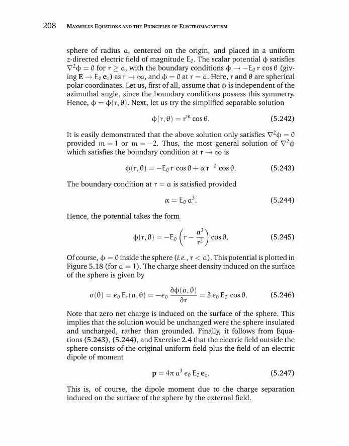
“chapter5” — 2007/11/29 — 15:40 — page 208 — #52
208 MAXWELL’S EQUATIONS AND THE PRINCIPLES OF ELECTROMAGNETISM
sphere of radius a, centered on the origin, and placed in a uniformz-directed electric field of magnitude E0. The scalar potential φ satisfies∇2φ = 0 for r ≥ a, with the boundary conditions φ → −E0 r cos θ (giv-ing E → E0 ez) as r → ∞, and φ = 0 at r = a. Here, r and θ are sphericalpolar coordinates. Let us, first of all, assume that φ is independent of theazimuthal angle, since the boundary conditions possess this symmetry.Hence, φ = φ(r, θ). Next, let us try the simplified separable solution
φ(r, θ) = rm cos θ. (5.242)
It is easily demonstrated that the above solution only satisfies ∇2φ = 0
provided m = 1 or m = −2. Thus, the most general solution of ∇2φ
which satisfies the boundary condition at r → ∞ is
φ(r, θ) = −E0 r cos θ+ α r−2 cos θ. (5.243)
The boundary condition at r = a is satisfied provided
α = E0 a3. (5.244)
Hence, the potential takes the form
φ(r, θ) = −E0
(r−
a3
r2
)cos θ. (5.245)
Of course,φ = 0 inside the sphere (i.e., r < a). This potential is plotted inFigure 5.18 (for a = 1). The charge sheet density induced on the surfaceof the sphere is given by
σ(θ) = ε0 Er(a, θ) = −ε0∂φ(a, θ)
∂r= 3 ε0 E0 cos θ. (5.246)
Note that zero net charge is induced on the surface of the sphere. Thisimplies that the solution would be unchanged were the sphere insulatedand uncharged, rather than grounded. Finally, it follows from Equa-tions (5.243), (5.244), and Exercise 2.4 that the electric field outside thesphere consists of the original uniform field plus the field of an electricdipole of moment
p = 4πa3 ε0 E0 ez. (5.247)
This is, of course, the dipole moment due to the charge separationinduced on the surface of the sphere by the external field.
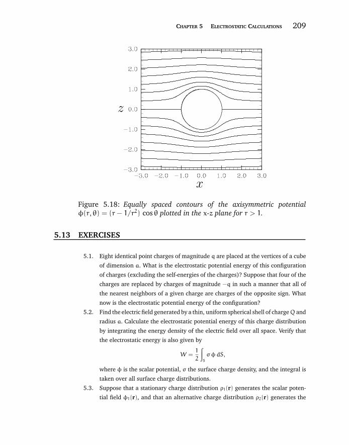
“chapter5” — 2007/11/29 — 15:40 — page 209 — #53
CHAPTER 5 ELECTROSTATIC CALCULATIONS 209
x
z
Figure 5.18: Equally spaced contours of the axisymmetric potentialφ(r, θ) = (r− 1/r2) cos θ plotted in the x-z plane for r > 1.
5.13 EXERCISES
5.1. Eight identical point charges of magnitude q are placed at the vertices of a cube
of dimension a. What is the electrostatic potential energy of this configuration
of charges (excluding the self-energies of the charges)? Suppose that four of the
charges are replaced by charges of magnitude −q in such a manner that all of
the nearest neighbors of a given charge are charges of the opposite sign. What
now is the electrostatic potential energy of the configuration?
5.2. Find the electric field generated by a thin, uniform spherical shell of chargeQ and
radius a. Calculate the electrostatic potential energy of this charge distribution
by integrating the energy density of the electric field over all space. Verify that
the electrostatic energy is also given by
W =1
2
∫
S
σφdS,
where φ is the scalar potential, σ the surface charge density, and the integral is
taken over all surface charge distributions.
5.3. Suppose that a stationary charge distribution ρ1(r) generates the scalar poten-
tial field φ1(r), and that an alternative charge distribution ρ2(r) generates the
“chapter5” — 2007/11/29 — 15:40 — page 210 — #54
210 MAXWELL’S EQUATIONS AND THE PRINCIPLES OF ELECTROMAGNETISM
potential φ2(r). Here, both charge distributions are assumed to be sufficiently
localized that the potential fields they generate go to zero at large distances.
Prove Green’s reciprocity theorem:∫φ1 ρ2 dV =
∫φ2 ρ1 dV,
where the volume integral is over all space. Hint: Use Maxwell’s equations and
the divergence theorem.
5.4. Two grounded, infinite, parallel conducting plates are separated by a perpendic-
ular distance d. A point charge q is placed between the plates. Demonstrate that
the total charge induced on one of the plates is (−q) times the fractional per-
pendicular distance of the point charge from the other plate. Hint: Use Green’s
reciprocity theorem.
5.5. Two grounded, concentric, thin spherical conducting shells have radii a and b,
where b > a. A point chargeq is placed between the shells at radius r (wherea <
r < b). Find the total charge induced on each shell. Hint: Use Green’s reciprocity
theorem.
5.6. Consider two insulated conductors, labeled 1 and 2. Let φ1 be the potential
of the first conductor when it is uncharged and the second conductor holds a
charge Q. Likewise, let φ2 be the potential of the second conductor when it
is uncharged and the first conductor holds a charge Q. Use Green’s reciprocity
theorem to demonstrate that
φ1 = φ2.
5.7. Consider two insulated spherical conductors. Let the first have radius a. Let the
second be sufficiently small that it can effectively be treated as a point charge,
and let it also be located a distance b > a from the center of the first. Suppose
that the first conductor is uncharged, and that the second carries a charge q.
What is the potential of the first conductor? Hint: Consider the result proved in
the previous exercise.
5.8. Consider a set of N conductors distributed in a vacuum. Suppose that the ith
conductor carries the charge Qi and is at the scalar potential φi. It follows from
the linearity of Maxwell’s equations and Ohm’s law that a linear relationship
exists between the potentials and the charges: i.e.,
φi =∑
j=1,N
pij Qj.
Here, the pij are termed the coefficients of potential. Demonstrate that pij = pji
for all i, j. Hint: Consider the result proved in Exercise 5.6. Show that the total
“chapter5” — 2007/11/29 — 15:40 — page 211 — #55
CHAPTER 5 ELECTROSTATIC CALCULATIONS 211
electrostatic potential energy of the charged conductors is
W =1
2
∑
i,j=1,N
pij Qi Qj.
5.9. Find the coefficients of potential for two thin, concentric, spherical conducting
shells of radius r1 and r2, where r2 > r1. Suppose thatQ1 andQ2 are the charges
on the inner and outer conductors, respectively. Calculate the electrostatic
potential energy of the system.
5.10. Returning to the problem discussed in Exercise 5.7, suppose that the first con-
ductor is now earthed, rather than being insulated and uncharged. What charge
is induced on the first conductor by the charge on the second? Hint: Consider
the concept of coefficient of potential.
5.11. Consider two separate conductors, the first of which is insulated and uncharged,
and the second of which is earthed. Prove that the first conductor is also at zero
(i.e., earth) potential. Hint: Consider the previous hint.
5.12. Consider a flat annular plate (e.g., a washer) of uniform thickness δ, inner radius
a, and outer radius b. Let the plate be fabricated from metal of uniform resistivity
η. Suppose that an electrical current I is fed into the plate symmetrically at
its inner radius, and extracted symmetrically at its outer radius. What is the
resistance of the plate? What is the rate of ohmic heating of the plate?
5.13. Consider an infinite uniform network of identical resistors of resistance R. Let
four resistors come together at each junction of the network (i.e., let the network
have a square lattice). Suppose that current is fed into a given junction and
extracted from a nearest neighbor junction. What is the effective resistance of
the network?
5.14. According to the uniqueness theorem, Poisson’s equation ∇2φ = −ρ/ε0 can only
have one solution if ρ is given in some volume V , and φ is specified on the
bounding surface S. Demonstrate that two solutions can differ by, at most, a
constant if the normal derivative of the potential, rather than the potential itself,
is specified on the bounding surface.
5.15. Consider a point charge q which is placed inside a thin, grounded, spherical
conducting shell of radius a a distance r from its center. Use the method of
images to find the surface charge density induced on the inside of the shell. What
is the net charge induced on the inside of the shell? What is the magnitude and
direction of the force of attraction between the the charge and the shell? What
electric field is induced outside the shell. How would these results be modified if
the sphere were (a) uncharged and insulated, or (b) maintained at the constant
potential V?
“chapter5” — 2007/11/29 — 15:40 — page 212 — #56
212 MAXWELL’S EQUATIONS AND THE PRINCIPLES OF ELECTROMAGNETISM
5.16. Using the method of images, show that the force of attraction, or repulsion,
between a point chargeq and an insulated conducting sphere of radiusa carrying
a charge Q is
f =q
4πε0
[Q + (a/d)q
d2−
aq
d (d − a2/d2)
],
where d > a is the distance of the charge from the center of the sphere. Demon-
strate that whenQ and q are of the same sign then the force is attractive provided
that
Q
d<
ad2
(d2 − a2)2−a
d.
5.17. An infinitely long conducting cylinder carries a charge per unit length λ and
runs parallel to an infinite grounded conducting plane. Let the radius of the
cylinder be a, and let the perpendicular distance between the cylinder’s axis and
the plane be d (where d > a). What is the force of attraction per unit length
between the cylinder and the plane? What is the charge per unit length induced
on the plane? Use the method of images.
5.18. A point charge q is located between two parallel, grounded, infinite conducting
planes separated by a perpendicular distance d. Suppose that the perpendicular
distance of the charge from one of the planes is x. Find the locations of the
infinite number of image charges, and, hence, express the force exerted on the
charge as an infinite series. Plot the magnitude of this force as a function of
x/d. Find expressions for the net charges induced on the two planes. Plot these
expressions as functions of x/d.
5.19. Two semi-infinite grounded conducting planes meet at right angles. A charge
q is located a perpendicular distance a from one, and b from another. Use the
method of images to find the magnitude and direction of the force of attraction
between the planes and the charge. What is the net charge induced on the
planes?
5.20. Two semi-infinite grounded conducting planes meet at sixty degrees. A charge
q is located the same perpendicular distance a from both. Use the method of
images to find the magnitude and direction of the force of attraction between
the planes and the charge. What is the net charge induced on the planes?
5.21. Find the function F(z), where z is the complex variable, whose real part can be
interpreted as the scalar potential associated with (a) a uniform electric field of
magnitude E0 directed along the x-axis, (b) a uniform electric field of magnitude
E0 directed along the y-axis, and (c) a line charge of charge per unit length λ
located at the origin.
“chapter5” — 2007/11/29 — 15:40 — page 213 — #57
CHAPTER 5 ELECTROSTATIC CALCULATIONS 213
5.22. Two semi-infinite conducting plates meet at 90, and are both held at the con-
stant potential V . Use complex analysis to find the variation of the surface charge
density with perpendicular distance from the vertex on both sides of the plates.
5.23. Two semi-infinite conducting plates meet at 60, and are both held at the con-
stant potential V . Use complex analysis to find the variation of the surface charge
density with perpendicular distance from the vertex on both sides of the plates.
5.24. Consider the complex function F(z) defined implicitly by the equation
i z = i F(z) + e i F(z).
Suppose that the real part of this function is interpreted as an electric poten-
tial. Plot the contours of this potential. What problem in electrostatics does this
potential best describe?
5.25. Consider an empty cubic box of dimensionawith conducting walls. Two opposite
walls are held at the constant potential V , whilst the other walls are earthed.
Find an expression for the electric potential inside the box. (Assume that the box
is centered on the origin, that the walls are all normal to one of the Cartesian
axes, and that the non-grounded walls are normal to the x-axis.) Suppose that
the two walls normal to the x-axis are held at potentials ±V . What now is the
potential inside the box? Use separation of variables.

“chapter5” — 2007/11/29 — 15:40 — page 214 — #58
“chapter6” — 2007/12/14 — 12:05 — page 215 — #1
C h a p t e r 6 DIELECTRIC ANDMAGNETIC MEDIA
6.1 INTRODUCTION
In this chapter, we shall use Maxwell’s equations to investigate the inter-action of dielectric and magnetic media with quasi-static electric andmagnetic fields.
6.2 POLARIZATION
The terrestrial environment is characterized by dielectric media (e.g., air,water) which are, for the most part, electrically neutral, since they aremade up of neutral atoms and molecules. However, if these atoms andmolecules are placed in an external electric field then they tend to polar-ize: i.e., their positively and negatively charged components displacewith respect to one another. Suppose that if a given neutral moleculeis placed in an external electric field E then the center of charge of itsconstituent electrons, whose total charge is (say) q, displaces by d withrespect to the center of charge of its constituent atomic nuclii. The dipolemoment of the molecule is defined as p = qd. If a dielectric medium ismade up of N such molecules per unit volume then the electric polariza-tion, P, of the medium (i.e., the dipole moment per unit volume) is givenby P = Np. More generally,
P(r) =∑i
Ni 〈pi〉, (6.1)
where 〈pi〉 is the average dipole moment of the ith type of moleculemaking up the medium, and Ni the average number of such moleculesper unit volume, in the vicinity of point r.
Now, we saw previously, in Exercise 3.4, that the scalar electricpotential field generated by an electric dipole of moment p situated atthe origin is
φ(r) =p · r4πε0 r3
. (6.2)
215
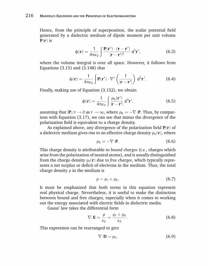
“chapter6” — 2007/12/14 — 12:05 — page 216 — #2
216 MAXWELL’S EQUATIONS AND THE PRINCIPLES OF ELECTROMAGNETISM
Hence, from the principle of superposition, the scalar potential fieldgenerated by a dielectric medium of dipole moment per unit volumeP(r) is
φ(r) =1
4πε0
∫P(r ′) · (r − r ′)
|r − r ′|3d3r ′, (6.3)
where the volume integral is over all space. However, it follows fromEquations (3.15) and (3.148) that
φ(r) =1
4πε0
∫P(r ′) · ∇ ′
(1
|r − r ′|
)d3r ′. (6.4)
Finally, making use of Equation (3.152), we obtain
φ(r) =1
4πε0
∫ρb(r ′)|r − r ′|
d3r ′, (6.5)
assuming that |P|/r → 0 as r → ∞, where ρb = −∇·P. Thus, by compar-ison with Equation (3.17), we can see that minus the divergence of thepolarization field is equivalent to a charge density.
As explained above, any divergence of the polarization field P(r) ofa dielectric medium gives rise to an effective charge density ρb(r), where
ρb = −∇·P. (6.6)
This charge density is attributable to bound charges (i.e., charges whicharise from the polarization of neutral atoms), and is usually distinguishedfrom the charge density ρf(r) due to free charges, which typically repre-sents a net surplus or deficit of electrons in the medium. Thus, the totalcharge density ρ in the medium is
ρ = ρf + ρb. (6.7)
It must be emphasized that both terms in this equation representreal physical charge. Nevertheless, it is useful to make the distinctionbetween bound and free charges, especially when it comes to workingout the energy associated with electric fields in dielectric media.
Gauss’ law takes the differential form
∇·E =ρ
ε0=ρf + ρbε0
. (6.8)
This expression can be rearranged to give
∇·D = ρf, (6.9)

“chapter6” — 2007/12/14 — 12:05 — page 217 — #3
CHAPTER 6 DIELECTRIC AND MAGNETIC MEDIA 217
where
D = ε0 E + P (6.10)
is termed the electric displacement, and has the same dimensions as P(i.e., dipole moment per unit volume). Gauss’ theorem tells us that∮
S
D·dS =
∫V
ρf dV. (6.11)
In other words, the flux of D out of some closed surface S is equal to thetotal free charge enclosed within that surface. Unlike the electric field E(which is the electric force acting on a unit charge), or the polarization P(which is the dipole moment per unit volume), the electric displacementD has no clear physical interpretation. In fact, the only reason for intro-ducing this quantity is that it enables us to calculate electric fields in thepresence of dielectric media without having to know the distribution ofbound charges beforehand. However, this is only possible if we have aconstitutive relation connecting E and D.
6.3 ELECTRIC SUSCEPTIBILITY AND PERMITTIVITY
In a large class of dielectric materials, there exits an approximately linearrelationship between P and E. If the material is isotropic then
P = ε0 χe E, (6.12)
where χe is termed the electric susceptibility. It follows that
D = ε0 εE, (6.13)
where
ε = 1+ χe (6.14)
is termed the relative dielectric constant or relative permittivity of themedium. (Likewise, ε0 is termed the permittivity of free space.) Note thatε is dimensionless. Values of ε for some common dielectric materials aregiven in Table 6.1. It can be seen that dielectric constants are generallygreater than unity, and can be significantly greater than unity for liquidsand solids.
It follows from Equations (6.9) and (6.13) that
∇·E =ρf
ε0 ε. (6.15)
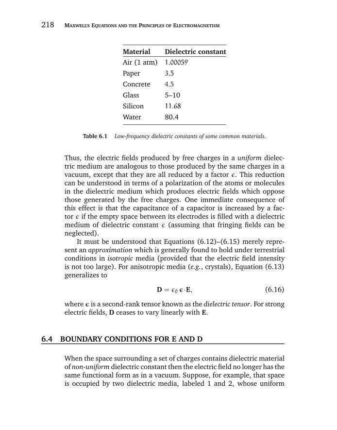
“chapter6” — 2007/12/14 — 12:05 — page 218 — #4
218 MAXWELL’S EQUATIONS AND THE PRINCIPLES OF ELECTROMAGNETISM
Material Dielectric constant
Air (1 atm) 1.00059
Paper 3.5
Concrete 4.5
Glass 5–10
Silicon 11.68
Water 80.4
Table 6.1 Low-frequency dielectric constants of some common materials.
Thus, the electric fields produced by free charges in a uniform dielec-tric medium are analogous to those produced by the same charges in avacuum, except that they are all reduced by a factor ε. This reductioncan be understood in terms of a polarization of the atoms or moleculesin the dielectric medium which produces electric fields which opposethose generated by the free charges. One immediate consequence ofthis effect is that the capacitance of a capacitor is increased by a fac-tor ε if the empty space between its electrodes is filled with a dielectricmedium of dielectric constant ε (assuming that fringing fields can beneglected).
It must be understood that Equations (6.12)–(6.15) merely repre-sent an approximation which is generally found to hold under terrestrialconditions in isotropic media (provided that the electric field intensityis not too large). For anisotropic media (e.g., crystals), Equation (6.13)generalizes to
D = ε0 ε·E, (6.16)
where ε is a second-rank tensor known as the dielectric tensor. For strongelectric fields, D ceases to vary linearly with E.
6.4 BOUNDARY CONDITIONS FOR E AND D
When the space surrounding a set of charges contains dielectric materialof non-uniform dielectric constant then the electric field no longer has thesame functional form as in a vacuum. Suppose, for example, that spaceis occupied by two dielectric media, labeled 1 and 2, whose uniform
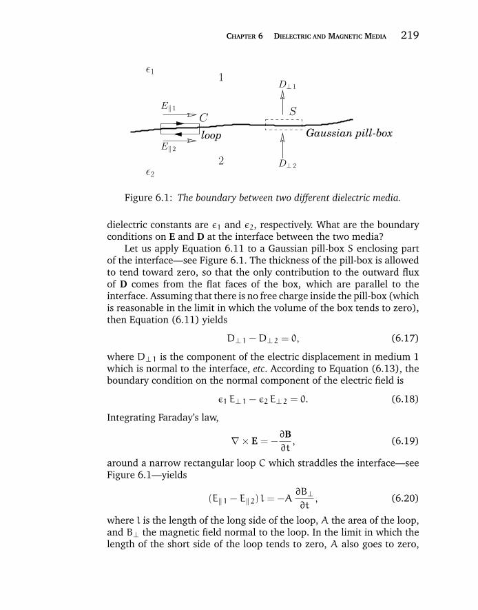
“chapter6” — 2007/12/14 — 12:05 — page 219 — #5
CHAPTER 6 DIELECTRIC AND MAGNETIC MEDIA 219
loop Gaussian pill-box.
2
SC
E‖ 1
E‖ 2
1D⊥ 1
D⊥ 2
ε1
ε2
Figure 6.1: The boundary between two different dielectric media.
dielectric constants are ε1 and ε2, respectively. What are the boundaryconditions on E and D at the interface between the two media?
Let us apply Equation 6.11 to a Gaussian pill-box S enclosing partof the interface—see Figure 6.1. The thickness of the pill-box is allowedto tend toward zero, so that the only contribution to the outward fluxof D comes from the flat faces of the box, which are parallel to theinterface. Assuming that there is no free charge inside the pill-box (whichis reasonable in the limit in which the volume of the box tends to zero),then Equation (6.11) yields
D⊥ 1 −D⊥ 2 = 0, (6.17)
where D⊥ 1 is the component of the electric displacement in medium 1which is normal to the interface, etc. According to Equation (6.13), theboundary condition on the normal component of the electric field is
ε1 E⊥ 1 − ε2 E⊥ 2 = 0. (6.18)
Integrating Faraday’s law,
∇ × E = −∂B∂t, (6.19)
around a narrow rectangular loop C which straddles the interface—seeFigure 6.1—yields
(E‖ 1 − E‖ 2) l = −A∂B⊥∂t
, (6.20)
where l is the length of the long side of the loop, A the area of the loop,and B⊥ the magnetic field normal to the loop. In the limit in which thelength of the short side of the loop tends to zero, A also goes to zero,
“chapter6” — 2007/12/14 — 12:05 — page 220 — #6
220 MAXWELL’S EQUATIONS AND THE PRINCIPLES OF ELECTROMAGNETISM
and we obtain the familiar boundary condition
E‖ 1 − E‖ 2 = 0. (6.21)
Generally speaking, there is a bound charge sheet on the interfacebetween two dielectric media. The charge density of this sheet followsfrom Gauss’ law:
σb = ε0 (E⊥ 1 − E⊥ 2) = (1/ε1 − 1/ε2)D⊥. (6.22)
This can also be written
σb = (P1 − P2) · n, (6.23)
where n is the unit normal at the interface (pointing from medium 1 tomedium 2), and P1,2 are the electric polarizations in the two media.
6.5 BOUNDARY VALUE PROBLEMS WITH DIELECTRICS
Consider a point charge q embedded in a semi-infinite dielectric mediumof uniform dielectric constant ε1, and located a distance d away from aplane interface which separates this medium from another semi-infinitedielectric medium of dielectric constant ε2. Let the interface coincidewith the plane z = 0, and let the point charge lie on the positive z-axis.In order to solve this problem, we need to find solutions to the equations
ε1∇·E =q δ(r − r0)
ε0, (6.24)
where r0 = (0, 0, d), for z > 0,
ε2∇·E = 0 (6.25)
for z < 0, and
∇ × E = 0 (6.26)
everywhere, subject to the boundary conditions
ε1 Ez(x, y, 0+) = ε2 Ez(x, y, 0−), (6.27)
Ex(x, y, 0+) = Ex(x, y, 0−), (6.28)
Ey(z, y, 0+) = Ey(x, y, 0−). (6.29)
We can solve this problem by employing a slightly modified form ofthe method of images—see Section 5.10. Since ∇ × E = 0 everywhere,
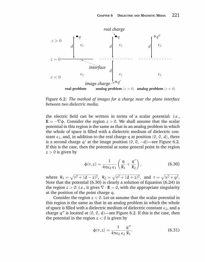
“chapter6” — 2007/12/14 — 12:05 — page 221 — #7
CHAPTER 6 DIELECTRIC AND MAGNETIC MEDIA 221
ε2d
interface
z > 0
z = 0
z < 0
real charge
q′
q q q′′
d d
d
real problem analog problem (z > 0) analog problem (z < 0)
ε1 ε1
image charge
ε2 ε1 ε2
Figure 6.2: The method of images for a charge near the plane interfacebetween two dielectric media.
the electric field can be written in terms of a scalar potential: i.e.,E = −∇φ. Consider the region z > 0. We shall assume that the scalarpotential in this region is the same as that in an analog problem in whichthe whole of space is filled with a dielectric medium of dielectric con-stant ε1, and, in addition to the real charge q at position (0, 0, d), thereis a second charge q ′ at the image position (0, 0, −d)—see Figure 6.2.If this is the case, then the potential at some general point in the regionz > 0 is given by
φ(r, z) =1
4πε0 ε1
(q
R1+q ′
R2
), (6.30)
where R1 =√r2 + (d− z)2, R2 =
√r2 + (d+ z)2, and r =
√x2 + y2.
Note that the potential (6.30) is clearly a solution of Equation (6.24) inthe region z > 0: i.e., it gives ∇ · E = 0, with the appropriate singularityat the position of the point charge q.
Consider the region z < 0. Let us assume that the scalar potential inthis region is the same as that in an analog problem in which the wholeof space is filled with a dielectric medium of dielectric constant ε2, and acharge q ′′ is located at (0, 0, d)—see Figure 6.2. If this is the case, thenthe potential in the region z < 0 is given by
φ(r, z) =1
4πε0 ε2
q ′′
R1. (6.31)
“chapter6” — 2007/12/14 — 12:05 — page 222 — #8
222 MAXWELL’S EQUATIONS AND THE PRINCIPLES OF ELECTROMAGNETISM
The above potential is clearly a solution of Equation (6.25) in the regionz < 0: i.e., it gives ∇·E = 0, with no singularities.
It now remains to choose q ′ and q ′′ in such a manner that theboundary conditions (6.27)–(6.29) are satisfied. The boundary condi-tions (6.28) and (6.29) are obviously satisfied if the scalar potential iscontinuous at the interface between the two dielectric media: i.e., if
φ(r, 0+) = φ(r, 0−). (6.32)
The boundary condition (6.27) implies a jump in the normal derivativeof the scalar potential across the interface: i.e.,
ε1∂φ(r, 0+)
∂z= ε2
∂φ(r, 0−)
∂z. (6.33)
The first matching condition yields
q+ q ′
ε1=q ′′
ε2, (6.34)
whereas the second gives
q− q ′ = q ′′. (6.35)
Here, use has been made of
∂
∂z
(1
R1
)z=0
= −∂
∂z
(1
R2
)z=0
=d
(r2 + d2)3/2. (6.36)
Equations (6.34) and (6.35) imply that
q ′ = −
(ε2 − ε1ε2 + ε1
)q, (6.37)
q ′′ =
(2 ε2
ε2 + ε1
)q. (6.38)
Now, the bound charge density is given by ρb = −∇·P, however, wehave P = ε0 χe E inside both dielectric media. Hence, ∇ · P = ε0 χe∇·E =0, except at the location of the original point charge. We conclude thatthere is zero bound charge density in either dielectric medium. However,there is a bound charge sheet on the interface between the two media.In fact, the density of this sheet is given by
σb(r) = ε0 (Ez 1 − Ez 2)z=0. (6.39)
“chapter6” — 2007/12/14 — 12:05 — page 223 — #9
CHAPTER 6 DIELECTRIC AND MAGNETIC MEDIA 223
Hence,
σb(r) = ε0∂φ(r, 0−)
∂z− ε0
∂φ(r, 0+)
∂z= −
q
2π
(ε2 − ε1)
ε1(ε2 + ε1)
d
(r2 + d2)3/2.
(6.40)
Incidentally, it is easily demonstrated that the net charge on the interfaceis q ′/ε1. In the limit ε2 ε1, the dielectric with dielectric constant ε2behaves like a conductor (i.e., E → 0 in the region z < 0), and the boundsurface charge density on the interface approaches that obtained in thecase where the plane z = 0 coincides with a conducting surface—seeSection 5.10.
As a second example, consider a dielectric sphere of radius a, anduniform dielectric constant ε, placed in a uniform z-directed electricfield of magnitude E0. Suppose that the sphere is centered on the origin.Now, we can always write E = −∇φ for an electrostatic problem. In thepresent case, ∇ · E = 0 both inside and outside the sphere, since thereare no free charges, and the bound charge density is zero in a uniformdielectric medium (or a vacuum). Hence, the scalar potential satisfiesLaplace’s equation, ∇2φ = 0, throughout space. Adopting spherical polarcoordinates, (r, θ,ϕ), aligned along the z-axis, the boundary conditionsare that φ → −E0 r cos θ as r → ∞, and that φ is well-behaved at r = 0.At the surface of the sphere, r = a, the continuity of E‖ implies that φis continuous. Furthermore, the continuity of D⊥ = ε0 ε E⊥ leads to thematching condition
∂φ
∂r
∣∣∣∣r=a+
= ε∂φ
∂r
∣∣∣∣r=a−
. (6.41)
Let us try axisymmetric separable solutions of the form rm cos θ.It is easily demonstrated that such solutions satisfy Laplace’s equationprovided that m = 1 or m = −2. Hence, the most general solution toLaplace’s equation outside the sphere, which satisfies the boundarycondition at r → ∞, is
φ(r, θ) = −E0 r cos θ+ E0 αa3 cos θr2
. (6.42)
Likewise, the most general solution inside the sphere, which satisfies theboundary condition at r = 0, is
φ(r, θ) = −E1 r cos θ. (6.43)
“chapter6” — 2007/12/14 — 12:05 — page 224 — #10
224 MAXWELL’S EQUATIONS AND THE PRINCIPLES OF ELECTROMAGNETISM
The continuity of φ at r = a yields
E0 − E0 α = E1. (6.44)
Likewise, the matching condition (6.41) gives
E0 + 2 E0 α = εE1. (6.45)
Hence, we obtain
α =ε− 1
ε+ 2, (6.46)
E1 =3 E0
ε+ 2. (6.47)
Note that the electric field inside the sphere is uniform, parallel to theexternal electric field outside the sphere, and of magnitude E1. Moreover,E1 < E0 , provided that ε > 1—see Figure 6.3. The density of the boundcharge sheet on the surface of the sphere is
σb(θ) = −ε0
(∂φ
∂r
∣∣∣∣r=a+
−∂φ
∂r
∣∣∣∣r=a−
)= 3 ε0
(ε− 1
ε+ 2
)E0 cos θ. (6.48)
Finally, the electric field outside the sphere consists of the originaluniform field, plus the field of an electric dipole of moment
p = 4πa3 ε0
(ε− 1
ε+ 2
)E0 ez. (6.49)
This is simply the net induced dipole moment, p = (4/3)πa3 P, of thesphere, where P = ε0 (ε− 1)E1 ez.
As a final example, consider a spherical cavity, of radius a, inside auniform dielectric medium of dielectric constant ε, in the presence of az-directed electric field of magnitude E0. This problem is analogous tothe previous one, except that the matching condition (6.41) becomes
ε∂φ
∂r
∣∣∣∣r=a+
=∂φ
∂r
∣∣∣∣r=a−
. (6.50)
Hence, ε → 1/ε, and we obtain
α = −ε− 1
1+ 2 ε, (6.51)
E1 =3 εE0
1+ 2 ε. (6.52)
Note that the field inside the cavity is uniform, parallel to the externalelectric field outside the sphere, and of magnitudeE1. Moreover, E1 > E0,
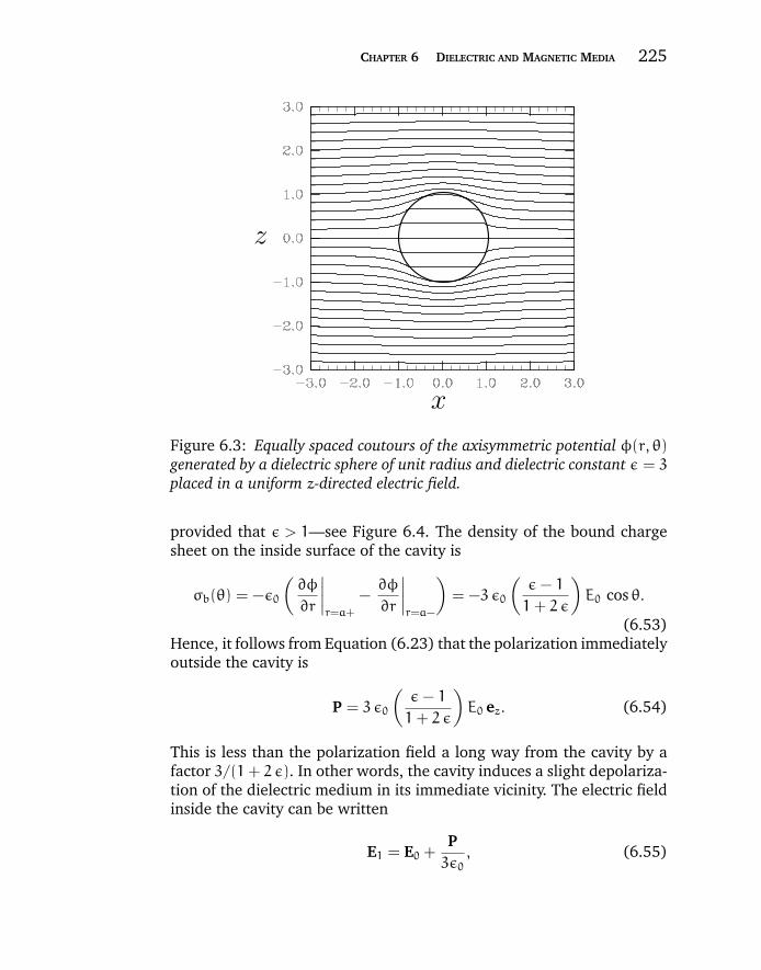
“chapter6” — 2007/12/14 — 12:05 — page 225 — #11
CHAPTER 6 DIELECTRIC AND MAGNETIC MEDIA 225
x
z
Figure 6.3: Equally spaced coutours of the axisymmetric potential φ(r, θ)generated by a dielectric sphere of unit radius and dielectric constant ε = 3
placed in a uniform z-directed electric field.
provided that ε > 1—see Figure 6.4. The density of the bound chargesheet on the inside surface of the cavity is
σb(θ) = −ε0
(∂φ
∂r
∣∣∣∣r=a+
−∂φ
∂r
∣∣∣∣r=a−
)= −3 ε0
(ε− 1
1+ 2 ε
)E0 cos θ.
(6.53)Hence, it follows from Equation (6.23) that the polarization immediatelyoutside the cavity is
P = 3 ε0
(ε− 1
1+ 2 ε
)E0 ez. (6.54)
This is less than the polarization field a long way from the cavity by afactor 3/(1+ 2 ε). In other words, the cavity induces a slight depolariza-tion of the dielectric medium in its immediate vicinity. The electric fieldinside the cavity can be written
E1 = E0 +P3ε0
, (6.55)

“chapter6” — 2007/12/14 — 12:05 — page 226 — #12
226 MAXWELL’S EQUATIONS AND THE PRINCIPLES OF ELECTROMAGNETISM
x
z
Figure 6.4: Equally spaced coutours of the axisymmetric potential φ(r, θ)generated by a cavity of unit radius inside a dielectric medium of dielectricconstant ε = 3 placed in a uniform z-directed electric field.
where E0 is the external field, and P the polarization field immediatelyoutside the cavity.
6.6 ENERGY DENSITY WITHIN A DIELECTRIC MEDIUM
Consider a system of free charges embedded in a dielectric medium. Theincrease in the total energy when a small amount of free charge δρf isadded to the system is given by
δW =
∫φδρf d
3r, (6.56)
where the integral is taken over all space, and φ(r) is the electro-static potential. Here, it is assumed that both the original charges andthe dielectric medium are held fixed, so that no mechanical work isperformed. It follows from Equation (6.9) that
δW =
∫φ∇·δDd3r, (6.57)
“chapter6” — 2007/12/14 — 12:05 — page 227 — #13
CHAPTER 6 DIELECTRIC AND MAGNETIC MEDIA 227
where δD is the change in the electric displacement associated with thecharge increment. Now the above equation can also be written
δW =
∫∇·(φδD)d3r −
∫∇φ·δDd3r, (6.58)
giving
δW =
∮S
φ δD·dS −
∫V
∇φ·δDd3r, (6.59)
where use has been made of Gauss’ theorem. Here, V is some volumebounded by the closed surface S. If the dielectric medium is of finitespatial extent then the surface term is eliminated by integrating over allspace. We thus obtain
δW = −
∫∇φ·δDd3r =
∫E·δDd3r. (6.60)
Now, this energy increment cannot be integrated unless E is a knownfunction of D. Let us adopt the conventional approach, and assume thatD = ε0 εE, where the dielectric constant ε is independent of the electricfield. The change in energy associated with taking the displacement fieldfrom zero to D(r) at all points in space is given by
W =
∫D
0δW =
∫D
0
∫E·δDd3r, (6.61)
or
W =
∫ ∫E0
ε0 ε δ(E2)
2d3r =
1
2
∫ε0 ε E
2 d3r, (6.62)
which reduces to
W =1
2
∫E·Dd3r. (6.63)
Thus, the electrostatic energy density inside a dielectric medium isgiven by
U =1
2E·D. (6.64)
This is a standard result, and is often quoted in textbooks. Nevertheless,it is important to realize that the above formula is only valid for dielec-tric media in which the electric displacement D varies linearly with theelectric field E. Note, finally, that Equation (6.64) is consistent with thepreviously obtained expression (5.20).
“chapter6” — 2007/12/14 — 12:05 — page 228 — #14
228 MAXWELL’S EQUATIONS AND THE PRINCIPLES OF ELECTROMAGNETISM
6.7 FORCE DENSITY WITHIN A DIELECTRIC MEDIUM
Equation (6.63) was derived by considering a virtual process in whichtrue charges are added to a system of charges and dielectrics which areheld fixed, so that no mechanical work is done against physical dis-placements. Let us now consider a different virtual process in whichthe physical coordinates of the charges and dielectric are given a vir-tual displacement δr at each point in space, but no free charges areadded to the system. Since we are dealing with a conservative system,the energy expression (6.63) can still be employed, despite the fact thatit was derived in terms of another virtual process. The variation in thetotal electrostatic energy δW when the system undergoes a virtual dis-placement δr is related to the electrostatic force density f acting withinthe dielectric medium via
δW = −
∫f ·δr d3r. (6.65)
So, if the medium is moving, and has a velocity field u, then the rate atwhich electrostatic energy is drained from the E and D fields is given by
dW
dt= −
∫f ·ud3r. (6.66)
Let us now consider the electrostatic energy increment due to achange δρf in the free charge distribution, and a change δε in the dielec-tric constant, both of which are caused by the virtual displacement. FromEquation (6.63),
δW =1
2ε0
∫ [D2 δ(1/ε) + 2D·δD/ε
]d3r, (6.67)
or
δW = −ε0
2
∫E2 δεd3r +
∫E·δDd3r. (6.68)
Here, the first term on the right-hand side represents the energy incre-ment due to the change in dielectric constant associated with the virtualdisplacement, whereas the second term corresponds to the energy incre-ment caused by the displacement of free charges. The second term canbe written∫
E·δDd3r = −
∫∇φ·δDd3r =
∫φ∇·δDd3r =
∫φδρf d
3r, (6.69)
“chapter6” — 2007/12/14 — 12:05 — page 229 — #15
CHAPTER 6 DIELECTRIC AND MAGNETIC MEDIA 229
where surface terms have been neglected. Thus, Equation (6.68) impliesthat
dW
dt=
∫ (φ∂ρf
∂t−ε0
2E2∂ε
∂t
)d3r. (6.70)
In order to arrive at an expression for the force density f , we needto express the time derivatives ∂ρ/∂t and ∂ε/∂t in terms of the velocityfield u. This can be achieved by adopting a dielectric equation of state:i.e., a relation which gives the dependence of the dielectric constant εon the mass density ρm. Let us assume that ε(ρm) is a known function.It follows that
Dε
Dt=dε
dρm
Dρm
Dt, (6.71)
where
D
Dt≡ ∂
∂t+ u·∇ (6.72)
is the total time derivative (i.e., the time derivative in a frame of refer-ence which is locally co-moving with the dielectric). The hydrodynamicequation of continuity of the dielectric is [see Equation (2.130)]
∂ρm
∂t+ ∇·(ρm u) = 0, (6.73)
which implies that
Dρm
Dt= −ρm∇·u. (6.74)
Hence, it follows that
∂ε
∂t= −
dε
dρmρm∇·u − u·∇ε. (6.75)
The conservation equation for the free charges is written
∂ρf
∂t+ ∇·(ρf u) = 0. (6.76)
Thus, we can express Equation (6.70) in the form
dW
dt=
∫ [−φ∇·(ρf u) +
ε0
2E2
dε
dρmρm∇·u +
(ε02E2∇ε
)·u]d3r.
(6.77)
“chapter6” — 2007/12/14 — 12:05 — page 230 — #16
230 MAXWELL’S EQUATIONS AND THE PRINCIPLES OF ELECTROMAGNETISM
Integrating the first term on the right-hand side by parts, and neglectingany surface contributions, we obtain
−
∫φ∇·(ρf u)d3r =
∫ρf∇φ·ud3r. (6.78)
Likewise,∫ε0
2E2
dε
dρmρm∇·ud3r = −
∫ε0
2∇(E2dε
dρmρm
)·ud3r. (6.79)
Hence, Equation (6.77) becomes
dW
dt=
∫ [−ρf E +
ε0
2E2∇ε−
ε0
2∇(E2
dε
dρmρm
)]·ud3r. (6.80)
Comparing with Equation (6.66), we can see that the force density insidethe dielectric medium is given by
f = ρf E −ε0
2E2∇ε+
ε0
2∇(E2dε
dρmρm
). (6.81)
The first term on the right-hand side of the above expression is the stan-dard electrostatic force density. The second term represents a force whichappears whenever an inhomogeneous dielectric is placed in an electricfield. The last term, which is known as the electrostriction term, corre-sponds to a force acting on a dielectric placed in an inhomogeneous elec-tric field. Note that the magnitude of the electrostriction force dependsexplicitly on the dielectric equation of state of the material, throughdε/dρm. The electrostriction term gives zero net force acting on anyfinite region of dielectric, if we can integrate over a large enough portionof the dielectric that its extremities lie in a field-free region. For this rea-son, the term is frequently neglected, since it usually does not contributeto the total force acting on a dielectric body. Note, however, that if theelectrostriction term is omitted then we obtain an incorrect pressure vari-ation within the dielectric, despite the fact that the total force is correct.
6.8 THE CLAUSIUS-MOSSOTTI RELATION
Let us now investigate what a dielectric equation of state actually lookslike. Suppose that a dielectric medium is made up of identical molecules
“chapter6” — 2007/12/14 — 12:05 — page 231 — #17
CHAPTER 6 DIELECTRIC AND MAGNETIC MEDIA 231
which develop a dipole moment
p = αε0 E (6.82)
when placed in an electric field E. The constant α (which has units ofvolume) is called the molecular polarizability. Note thatα, which is solelya property of the molecule, is typically of order the molecular volume.If N is the number density of molecules then the polarization of themedium is
P = Np = Nαε0 E, (6.83)
or
P =NA ρm α
Mε0 E, (6.84)
where ρm is the mass density, NA is Avogadro’s number, and M is themolecular weight. But, how does the electric field experienced by anindividual molecule relate to the average electric field in the medium?This is not a trivial question, since we expect the electric field to varystrongly (on atomic length-scales) inside the medium.
Suppose that the dielectric is polarized with a uniform mean elec-tric field E0 = E0 ez. Consider one of the molecules which constitute thedielectric. Let us draw a sphere of radiusa about this particular molecule.This is intended to represent the boundary between the microscopic andthe macroscopic range of phenomena affecting the molecule. We shalltreat the dielectric outside the sphere as a continuous medium, and thedielectric inside the sphere as a collection of polarized molecules. Notethat, unlike the case of a spherical cavity in a dielectric medium, there isno depolarization of the dielectric immediately outside the sphere, sincethere is dielectric material inside the sphere. Thus, from Equation (6.55),the total field inside the sphere is
E = E0 +P3ε0
, (6.85)
where P is given by Equation (6.84). The second term on the right-handside of the above equation is the field at the molecule due to the surfacecharge on the inside of the sphere.
The field due to the individual molecules within the sphere isobtained by summing over the dipole fields of these molecules. The elec-tric field at a distance r from a dipole of moment p is (see Exercise 3.4)
E = −1
4πε0
[pr3
−3 (p·r) rr5
]. (6.86)
“chapter6” — 2007/12/14 — 12:05 — page 232 — #18
232 MAXWELL’S EQUATIONS AND THE PRINCIPLES OF ELECTROMAGNETISM
It is assumed that the dipole moment of each molecule within the sphereis the same, and also that the molecules are evenly distributed through-out the sphere. This being the case, the value of Ez at the molecule dueto all of the other molecules within in the sphere,
Ez = −1
4πε0
∑ [pz r
2 − 3 (px x z+ py y z+ pz z2)
r5
], (6.87)
is zero, since
∑z2 =
1
3
∑r2 (6.88)
and ∑x z =
∑y z = 0. (6.89)
Here, the sum is over all of the molecules in the sphere. Furthermore,it is easily demonstrated that Eθ = Eϕ = 0 (where θ and ϕ are sphericalpolar coordinates). Hence, the electric field at the molecule due to theother molecules within the sphere vanishes.
It is clear that the net electric field seen by an individual molecule is
E = E0 +P3ε0
. (6.90)
This is larger than the average electric field E0 in the dielectric. Theabove analysis indicates that this effect is ascribable to the long range(rather than the short range) interactions of the molecule with theother molecules in the medium. Making use of Equation (6.84), andthe definition P = ε0 (ε− 1) E0, we obtain
ε− 1
ε+ 2=NA ρm α
3M. (6.91)
This formula is called the Clausius-Mossotti relation, and is found to workfairly well for relatively dilute dielectric media whose dielectric constantsare close to unity. Incidentally, the right-hand side of this expression isapproximately the volume fraction of space occupied by the moleculesmaking up the medium in question (and, should, therefore, be less thanunity). Finally, the Clausius-Mossotti relation yields
dε
dρm=
(ε− 1) (ε+ 2)
3 ρm. (6.92)
“chapter6” — 2007/12/14 — 12:05 — page 233 — #19
CHAPTER 6 DIELECTRIC AND MAGNETIC MEDIA 233
6.9 DIELECTRIC LIQUIDS IN ELECTROSTATIC FIELDS
Consider the behaviour of an uncharged dielectric liquid placed in anelectrostatic field. If p(r) is the pressure in the liquid when it is in equilib-rium with the electrostatic force density f(r), then force balance requiresthat
∇p = f . (6.93)
It follows from Equation (6.81) that
∇p = −ε0
2E2∇ε+
ε0
2∇(E2dε
dρmρm
)=ε0 ρm
2∇(E2dε
dρm
), (6.94)
since ∇ε = (dε/dρm)∇ρm. We can integrate this equation to give∫p2
p1
dp
ρm=ε0
2
([E2dε
dρm
]2
−
[E2dε
dρm
]1
), (6.95)
where 1 and 2 refer to two general points within the liquid. Here, it isassumed that the liquid possesses an equation of state, so that p = p(ρm).If the liquid is essentially incompressible (i.e., ρm constant) then
p2 − p1 =ε0 ρm
2
[E2
dε
dρm
]21
. (6.96)
Moreover, if the liquid obeys the Clausius-Mossotti relation then
p2 − p1 =
[ε0 E
2
2
(ε− 1) (ε+ 2)
3
]21
. (6.97)
According to Equations (6.47) and (6.97), if a sphere of dielectricliquid is placed in a uniform electric field E0 then the pressure inside theliquid takes the constant value
p =3
2ε0
(ε− 1
ε+ 2
)E20 . (6.98)
Now, it is fairly clear that the electrostatic forces acting on the dielectricare all concentrated at the edge of the sphere, and are directed radiallyinward: i.e., the dielectric is compressed by the external electric field.This is a somewhat surprising result, since the electrostatic forces actingon a rigid conducting sphere are also concentrated at the edge of the
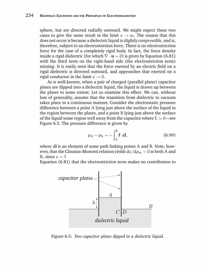
“chapter6” — 2007/12/14 — 12:05 — page 234 — #20
234 MAXWELL’S EQUATIONS AND THE PRINCIPLES OF ELECTROMAGNETISM
sphere, but are directed radially outward. We might expect these twocases to give the same result in the limit ε → ∞. The reason that thisdoes not occur is because a dielectric liquid is slightly compressible, and is,therefore, subject to an electrostriction force. There is no electrostrictionforce for the case of a completely rigid body. In fact, the force densityinside a rigid dielectric (for which ∇ · u = 0) is given by Equation (6.81)with the third term on the right-hand side (the electrostriction term)missing. It is easily seen that the force exerted by an electric field on arigid dielectric is directed outward, and approaches that exerted on arigid conductor in the limit ε → 0.
As is well-known, when a pair of charged (parallel plane) capacitorplates are dipped into a dielectric liquid, the liquid is drawn up betweenthe plates to some extent. Let us examine this effect. We can, withoutloss of generality, assume that the transition from dielectric to vacuumtakes place in a continuous manner. Consider the electrostatic pressuredifference between a point A lying just above the surface of the liquid inthe region between the plates, and a point B lying just above the surfaceof the liquid some region well away from the capacitor where E 0—seeFigure 6.5. The pressure difference is given by
pA − pB = −
∫BA
f ·dl, (6.99)
where dl is an element of some path linking points A and B. Note, how-ever, that the Clausius-Mossotti relation yields dε/dρm = 0 at bothA andB, since ε = 1 in a vacuum [see Equation (6.92)]. Thus, it is clear fromEquation (6.81) that the electrostriction term makes no contribution to
capacitor plates
A
B
dielectric liquid
h
C D
Figure 6.5: Two capacitor plates dipped in a dielectric liquid.
“chapter6” — 2007/12/14 — 12:05 — page 235 — #21
CHAPTER 6 DIELECTRIC AND MAGNETIC MEDIA 235
the line integral (6.99). It follows that
pA − pB =ε0
2
∫BA
E2∇ε·dl. (6.100)
The only contribution to this integral comes from the vacuum/dielectricinterface in the vicinity of point A (since ε is constant inside the liquid,and E 0 in the vicinity of point B). Suppose that the electric field atpoint A has normal and tangential (to the surface) components E⊥ andE‖, respectively. Making use of the boundary conditions that D⊥ and E‖are constant across a vacuum/dielectric interface, we obtain
pA − pB =ε0
2
[E2‖ (ε− 1) +
D2⊥ε20
∫ε1
dε
ε2
], (6.101)
giving
pA − pB =ε0 (ε− 1)
2
[E2‖ +
D2⊥
ε20 ε
]. (6.102)
This electrostatic pressure difference can be equated to the hydrostaticpressure difference ρm gh to determine the height h that the liquid risesbetween the plates. At first sight, the above analysis appears to suggestthat the dielectric liquid is drawn upward by a surface force acting on thevacuum/dielectric interface in the region between the plates. In fact,this is far from being the case. A brief examination of Equations (6.93)and (6.97) shows that this surface force is actually directed downward.Indeed, according to Equation (6.81), the force which causes the liquidto rise between the plates is a volume force which develops in the regionof non-uniform electric field at the base of the capacitor, where the fieldsplays out between the plates. Thus, although we can determine theheight to which the fluid rises between the plates without reference tothe electrostriction force, it is, somewhat paradoxically, this force whichis actually responsible for supporting the liquid against gravity.
Let us consider another paradox concerning the electrostatic forcesexerted in a dielectric medium. Suppose that we have two chargesembedded in a uniform dielectric medium of dielectric constant ε. Theelectric field generated by each charge is the same as that in vacuum,except that it is reduced by a factor ε. Therefore, we would expect thatthe force exerted by one charge on another is the same as that in vac-uum, except that it is also reduced by a factor ε. Let us examine how thisreduction in force comes about. Consider a simple example. Suppose

“chapter6” — 2007/12/14 — 12:05 — page 236 — #22
236 MAXWELL’S EQUATIONS AND THE PRINCIPLES OF ELECTROMAGNETISM
that we take a parallel plate capacitor, and insert a block of solid dielec-tric between the plates. Suppose, further, that there is a small vacuumgap between the faces of the block and each of the capacitor plates.Let ±σ be the surface charge densities on each of the capacitor plates,and let ±σb be the bound surface charge densities which develop on theouter faces of the intervening dielectric block. The two layers of polar-ization charge produce equal and opposite electric fields on each plate,and their effects therefore cancel each other. Thus, from the point ofview of electrical interaction alone, there would appear to be no changein the force exerted by one capacitor plate on the other when a dielectricslab is placed between them (assuming that σ remains constant dur-ing this process). That is, the force per unit area (which is attractive)remains
f =σ2
2ε0(6.103)
—see Equation (5.71). However, in experiments in which a capacitor issubmerged in a dielectric liquid, the force per unit area exerted by oneplate on another is observed to decrease to
f =σ2
2ε0 ε. (6.104)
This apparent paradox can be explained by taking into account thedifference in liquid pressure in the field-filled space between the plates,and the field-free region outside the capacitor. This pressure differenceis balanced by internal elastic forces in the case of a solid dielectric, butis transmitted to the plates in the case of the liquid. We can computethe pressure difference between a point C on the inside surface of oneof the capacitor plates, and a point D on the outside surface of the sameplate using Equation (6.100)—see Figure 6.5. If we neglect end effects,then the electric field is normal to the plates in the region between theplates, and is zero everywhere else. Thus, the only contribution to theline integral (6.100) comes from the plate/dielectric interface in thevicinity of point C. Adopting Equation (6.102), we find that
pC − pD =ε0
2
(1−
1
ε
)E2⊥ =
σ2
2ε0
(1−
1
ε
), (6.105)
where E⊥ = σ/ε0 is the normal field strength between the plates in theabsence of the dielectric. The sum of this pressure force (which is repul-sive) and the attractive electrostatic force per unit area (6.103) yields a
“chapter6” — 2007/12/14 — 12:05 — page 237 — #23
CHAPTER 6 DIELECTRIC AND MAGNETIC MEDIA 237
net attractive force per unit area of
f =σ2
2ε0 ε(6.106)
acting between the plates. Thus, any decrease in the forces exerted bycharges on one another when they are immersed, or embedded, in adielectric medium can only be understood in terms of mechanical forcestransmitted between the charges by the medium itself.
6.10 POLARIZATION CURRENT
We have seen that the bound charge density is related to the polarizationfield via
ρb = −∇ · P. (6.107)
Now, it is clear, from this equation, that if the polarization field insidesome dielectric material changes in time then the distribution of boundcharges will also change. Hence, in order to conserve charge, a netcurrent must flow. This current is known as the polarization current.Charge conservation implies that
∇ · jp +∂ρb
∂t= 0, (6.108)
where jp is the polarization current density. It follows from the previoustwo equations that
jp =∂P∂t. (6.109)
Note that the polarization current is a real current, despite the fact thatit is generated by the rearrangement of bound charges. There is, how-ever, no drifting of real charges over length-scales longer than atomic ormolecular length-scales associated with this current.
6.11 MAGNETIZATION
All matter is built up out of molecules, and each molecule consists ofelectrons in motion around stationary nuclii. The currents associatedwith this type of electron motion are termed molecular currents. Each
“chapter6” — 2007/12/14 — 12:05 — page 238 — #24
238 MAXWELL’S EQUATIONS AND THE PRINCIPLES OF ELECTROMAGNETISM
molecular current is a tiny closed circuit of atomic dimensions, andmay therefore be appropriately described as a magnetic dipole. Sup-pose that a given molecule has a magnetic dipole moment m. If thereareN such molecules per unit volume then the magnetization M (i.e., themagnetic dipole moment per unit volume) is given by M = Nm. Moregenerally,
M(r) =∑i
Ni 〈mi〉, (6.110)
where 〈mi〉 is the average magnetic dipole moment of the ith type ofmolecule, and Ni is the average number of such molecules per unitvolume, in the vicinity of point r.
Now, we saw earlier, in Exercise 3.20, that the vector potential fieldgenerated by a magnetic dipole of moment m situated at the origin is
A(r) =µ0
4π
m × rr3
. (6.111)
Hence, from the principle of superposition, the vector potential fieldgenerated by a magnetic medium of magnetic moment per unit volumeM(r) is
A(r) =µ0
4π
∫M(r ′) × (r − r ′)
|r − r ′|3d3r ′, (6.112)
where the volume integral is taken over all space. However, it followsfrom Equations (3.15) and (3.148) that
A(r) =µ0
4π
∫M(r ′) × ∇ ′
(1
|r − r ′|
)d3r ′. (6.113)
Now, it is easily demonstrated that∫f × ∇gd3r =
∫g∇ × f d3r, (6.114)
provided that the integral is over all space, and g |f | → 0 as |r| → ∞.Hence, for a magnetization field of finite extent, we can write
A(r) =µ0
2π
∫jm(r ′)|r − r ′|
d3r ′, (6.115)
where
jm = ∇ × M. (6.116)
“chapter6” — 2007/12/14 — 12:05 — page 239 — #25
CHAPTER 6 DIELECTRIC AND MAGNETIC MEDIA 239
It follows, by comparison with Equation (3.215), that the curl of themagnetization field constitutes a current density. The associated currentis known as the magnetization current.
The total current density, j, in a general medium takes the form
j = jt + ∇ × M +∂P∂t, (6.117)
where the three terms on the right-hand side represent the true currentdensity (i.e., that part of the current density which is due to the movementof free charges), the magnetization current density, and the polarizationcurrent density, respectively. It must be emphasized that all three termsrepresent real physical currents, although only the first term is due tothe motion of real charges (over more than molecular dimensions).
Now, the differential form of Ampere’s law is
∇ × B = µ0 j + µ0ε0∂E∂t, (6.118)
which can also be written
∇ × B = µ0 jt + µ0∇ × M + µ0∂D∂t, (6.119)
where use has been made of Equation (6.117) and the definition D =ε0 E + P. The above expression can be rearranged to give
∇ × H = jt +∂D∂t, (6.120)
where
H =Bµ0
− M (6.121)
is termed the magnetic intensity, and has the same dimensions as M (i.e.,magnetic dipole moment per unit volume). In a steady-state situation,Stokes’ theorem tell us that∮
C
H·dl =
∫S
jt ·dS. (6.122)
In other words, the line integral of H around some closed loop is equalto the flux of the true current through any surface attached to that loop.Unlike the magnetic field B (which specifies the magnetic force q v × Bacting on a charge q moving with velocity v), or the magnetization M(which is the magnetic dipole moment per unit volume), the magnetic
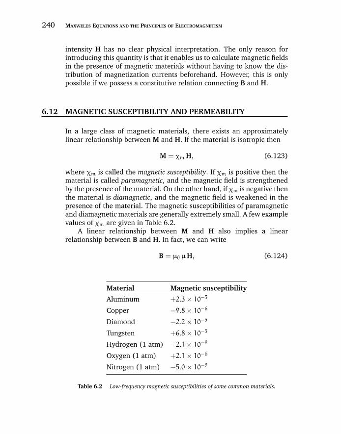
“chapter6” — 2007/12/14 — 12:05 — page 240 — #26
240 MAXWELL’S EQUATIONS AND THE PRINCIPLES OF ELECTROMAGNETISM
intensity H has no clear physical interpretation. The only reason forintroducing this quantity is that it enables us to calculate magnetic fieldsin the presence of magnetic materials without having to know the dis-tribution of magnetization currents beforehand. However, this is onlypossible if we possess a constitutive relation connecting B and H.
6.12 MAGNETIC SUSCEPTIBILITY AND PERMEABILITY
In a large class of magnetic materials, there exists an approximatelylinear relationship between M and H. If the material is isotropic then
M = χm H, (6.123)
where χm is called the magnetic susceptibility. If χm is positive then thematerial is called paramagnetic, and the magnetic field is strengthenedby the presence of the material. On the other hand, if χm is negative thenthe material is diamagnetic, and the magnetic field is weakened in thepresence of the material. The magnetic susceptibilities of paramagneticand diamagnetic materials are generally extremely small. A few examplevalues of χm are given in Table 6.2.
A linear relationship between M and H also implies a linearrelationship between B and H. In fact, we can write
B = µ0 µH, (6.124)
Material Magnetic susceptibility
Aluminum +2.3× 10⁻⁵
Copper −9.8× 10⁻⁶
Diamond −2.2× 10⁻⁵
Tungsten +6.8× 10⁻⁵
Hydrogen (1 atm) −2.1× 10⁻⁹
Oxygen (1 atm) +2.1× 10⁻⁶
Nitrogen (1 atm) −5.0× 10⁻⁹
Table 6.2 Low-frequency magnetic susceptibilities of some common materials.
“chapter6” — 2007/12/14 — 12:05 — page 241 — #27
CHAPTER 6 DIELECTRIC AND MAGNETIC MEDIA 241
where
µ = 1+ χm (6.125)
is termed the relative magnetic permeability of the material in question.(Likewise, µ0 is termed the permeability of free space.) Note that µ isdimensionless. It is clear from Table 6.2 that the relative permeabilitiesof common diamagnetic and paramagnetic materials do not differ sub-stantially from unity. In fact, to all intents and purposes, the magneticproperties of such materials can be safely neglected.
6.13 FERROMAGNETISM
There exists, however, a third class of magnetic materials called fer-romagnetic materials. Such materials are characterized by a possiblepermanent magnetization, and generally have a profound effect on mag-netic fields (i.e., µ 1). Unfortunately, ferromagnetic materials do notgenerally exhibit a linear dependence between M and H, or between Band H, so that we cannot employ Equations (6.123) and (6.124) withconstant values of χm and µ. It is still expedient to use Equation (6.124)as the definition of µ, with µ = µ(H). However, this practice can leadto difficulties under certain circumstances. The permeability of a ferro-magnetic material, as defined by Equation (6.124), can vary through theentire range of possible values from zero to infinity, and may be eitherpositive or negative. The most sensible approach is to consider eachproblem involving ferromagnetic materials separately, try to determinewhich region of the B-H diagram is important for the particular case inhand, and then make approximations appropriate to this region.
First, let us consider an unmagnetized sample of ferromagneticmaterial. If the magnetic intensity, which is initially zero, is increasedmonotonically, then the B-H relationship traces out a curve such as thatshown schematially in Figure 6.6. This is called a magnetization curve.It is evident that the permeabilities µ derived from the curve (accordingto the rule µ = µ−1
0 B/H) are always positive, and show a wide range ofvalues. The maximum permeability occurs at the “knee” of the curve. Insome materials, this maximum permeability is as large as 105. The rea-son for the knee is that the magnetization M reaches a maximum valuein the material, so that
B = µ0 (H + M) (6.126)
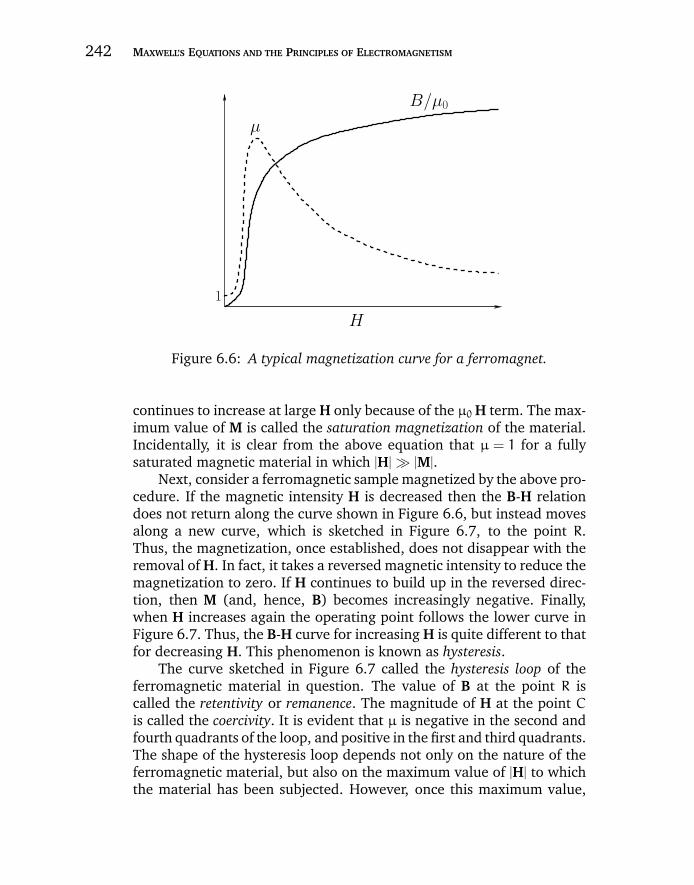
“chapter6” — 2007/12/14 — 12:05 — page 242 — #28
242 MAXWELL’S EQUATIONS AND THE PRINCIPLES OF ELECTROMAGNETISM
1
H
B/µ0
µ
Figure 6.6: A typical magnetization curve for a ferromagnet.
continues to increase at large H only because of the µ0 H term. The max-imum value of M is called the saturation magnetization of the material.Incidentally, it is clear from the above equation that µ = 1 for a fullysaturated magnetic material in which |H| |M|.
Next, consider a ferromagnetic sample magnetized by the above pro-cedure. If the magnetic intensity H is decreased then the B-H relationdoes not return along the curve shown in Figure 6.6, but instead movesalong a new curve, which is sketched in Figure 6.7, to the point R.Thus, the magnetization, once established, does not disappear with theremoval of H. In fact, it takes a reversed magnetic intensity to reduce themagnetization to zero. If H continues to build up in the reversed direc-tion, then M (and, hence, B) becomes increasingly negative. Finally,when H increases again the operating point follows the lower curve inFigure 6.7. Thus, the B-H curve for increasing H is quite different to thatfor decreasing H. This phenomenon is known as hysteresis.
The curve sketched in Figure 6.7 called the hysteresis loop of theferromagnetic material in question. The value of B at the point R iscalled the retentivity or remanence. The magnitude of H at the point Cis called the coercivity. It is evident that µ is negative in the second andfourth quadrants of the loop, and positive in the first and third quadrants.The shape of the hysteresis loop depends not only on the nature of theferromagnetic material, but also on the maximum value of |H| to whichthe material has been subjected. However, once this maximum value,
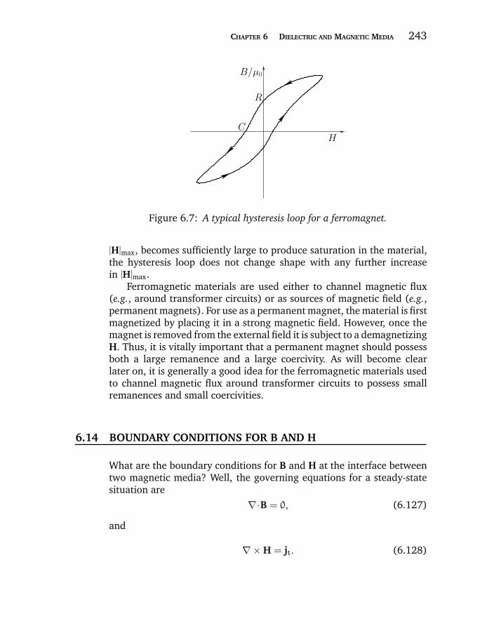
“chapter6” — 2007/12/14 — 12:05 — page 243 — #29
CHAPTER 6 DIELECTRIC AND MAGNETIC MEDIA 243
H
R
C
B/µ0
Figure 6.7: A typical hysteresis loop for a ferromagnet.
|H|max, becomes sufficiently large to produce saturation in the material,the hysteresis loop does not change shape with any further increasein |H|max.
Ferromagnetic materials are used either to channel magnetic flux(e.g., around transformer circuits) or as sources of magnetic field (e.g.,permanent magnets). For use as a permanent magnet, the material is firstmagnetized by placing it in a strong magnetic field. However, once themagnet is removed from the external field it is subject to a demagnetizingH. Thus, it is vitally important that a permanent magnet should possessboth a large remanence and a large coercivity. As will become clearlater on, it is generally a good idea for the ferromagnetic materials usedto channel magnetic flux around transformer circuits to possess smallremanences and small coercivities.
6.14 BOUNDARY CONDITIONS FOR B AND H
What are the boundary conditions for B and H at the interface betweentwo magnetic media? Well, the governing equations for a steady-statesituation are
∇·B = 0, (6.127)
and
∇ × H = jt. (6.128)
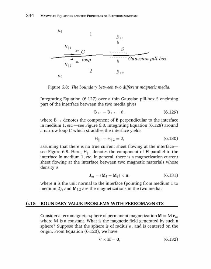
“chapter6” — 2007/12/14 — 12:05 — page 244 — #30
244 MAXWELL’S EQUATIONS AND THE PRINCIPLES OF ELECTROMAGNETISM
loop Gaussian pill-box.
H‖ 2
SC
1
2 B⊥ 2
B⊥ 1
µ1
µ2
H‖ 1
Figure 6.8: The boundary between two different magnetic media.
Integrating Equation (6.127) over a thin Gaussian pill-box S enclosingpart of the interface between the two media gives
B⊥ 1 − B⊥ 2 = 0, (6.129)
where B⊥ 1 denotes the component of B perpendicular to the interfacein medium 1, etc.—see Figure 6.8. Integrating Equation (6.128) arounda narrow loop C which straddles the interface yields
H‖ 1 −H‖ 2 = 0, (6.130)
assuming that there is no true current sheet flowing at the interface—see Figure 6.8. Here, H‖ 1 denotes the component of H parallel to theinterface in medium 1, etc. In general, there is a magnetization currentsheet flowing at the interface between two magnetic materials whosedensity is
Jm = (M1 − M2) × n, (6.131)
where n is the unit normal to the interface (pointing from medium 1 tomedium 2), and M1,2 are the magnetizations in the two media.
6.15 BOUNDARY VALUE PROBLEMS WITH FERROMAGNETS
Consider a ferromagnetic sphere of permanent magnetization M = M ez,where M is a constant. What is the magnetic field generated by such asphere? Suppose that the sphere is of radius a, and is centered on theorigin. From Equation (6.120), we have
∇ × H = 0, (6.132)
“chapter6” — 2007/12/14 — 12:05 — page 245 — #31
CHAPTER 6 DIELECTRIC AND MAGNETIC MEDIA 245
since this is a time-independent problem with no true currents. It followsthat
H = −∇φm, (6.133)
where φm is termed the magnetic scalar potential. Now,
H =Bµ0
− M, (6.134)
which implies that
∇ · H = 0 (6.135)
everywhere (apart from on the surface of the sphere), since ∇ · B = 0,and M is constant inside the sphere, and zero outside. It follows that themagnetic scalar potential satisfies Laplace’s equation,
∇2φm = 0, (6.136)
both inside and outside the sphere.Adopting spherical polar coordinates, (r, θ,ϕ), aligned along the z-
axis, the boundary conditions are that φm is well-behaved at r = 0, andφm → 0 as r → ∞. Moreover, Equation (6.130) implies that φm must becontinuous at r = a, whereas Equations (6.126) and (6.129) yield
−
[∂φm
∂r
]a+
a−
= M · er, (6.137)
or∂φm
∂r
∣∣∣∣r=a+
−∂φm
∂r
∣∣∣∣r=a−
= −M cos θ. (6.138)
Let us try separable solutions of the form rm cos θ. It is easily demon-strated that such solutions satisfy Laplace’s equation provided thatm = 1
or m = −2. Hence, the most general solution to Laplace’s equationoutside the sphere, which satisfies the boundary condition at r → ∞, is
φm(r, θ) = Ca3 cos θr2
. (6.139)
Likewise, the most general solution inside the sphere, which satisfies theboundary condition at r = 0, is
φm(r, θ) = Dr cos θ. (6.140)
The continuity of φm at r = a gives C = D, whereas the boundarycondition (6.138) yields C = M/3. Hence, the magnetic scalar potential
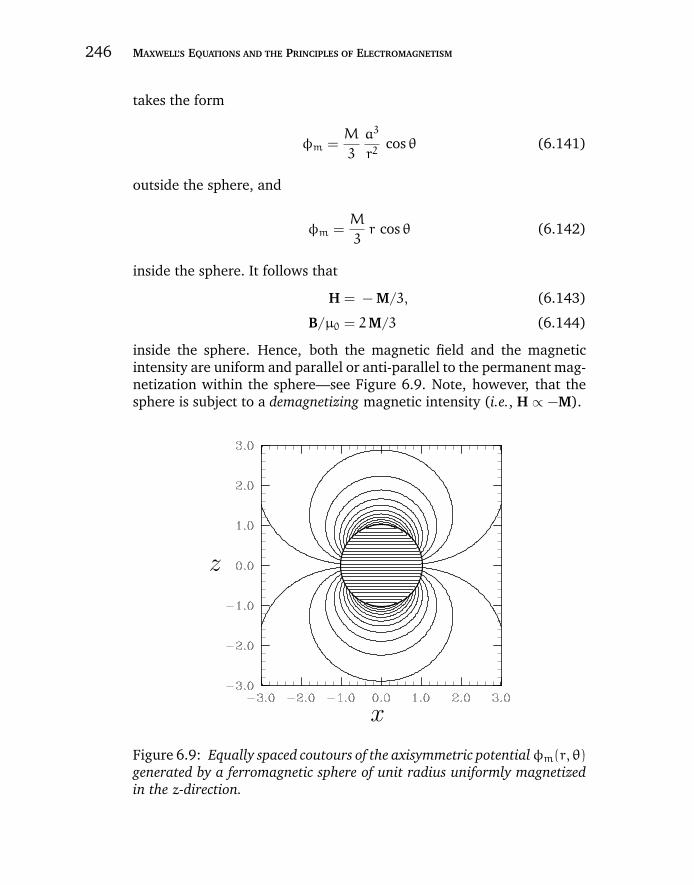
“chapter6” — 2007/12/14 — 12:05 — page 246 — #32
246 MAXWELL’S EQUATIONS AND THE PRINCIPLES OF ELECTROMAGNETISM
takes the form
φm =M
3
a3
r2cos θ (6.141)
outside the sphere, and
φm =M
3r cos θ (6.142)
inside the sphere. It follows that
H = − M/3, (6.143)
B/µ0 = 2M/3 (6.144)
inside the sphere. Hence, both the magnetic field and the magneticintensity are uniform and parallel or anti-parallel to the permanent mag-netization within the sphere—see Figure 6.9. Note, however, that thesphere is subject to a demagnetizing magnetic intensity (i.e., H ∝ −M).
x
z
Figure 6.9: Equally spaced coutours of the axisymmetric potentialφm(r, θ)generated by a ferromagnetic sphere of unit radius uniformly magnetizedin the z-direction.

“chapter6” — 2007/12/14 — 12:05 — page 247 — #33
CHAPTER 6 DIELECTRIC AND MAGNETIC MEDIA 247
It is easily demonstrated that the scalar magnetic potential due to amagnetic dipole of moment m at the origin is
φm(r) =1
4π
m · rr3
. (6.145)
Thus, it is clear that the magnetic field outside the sphere is the same asthat of a magnetic dipole of moment
m =4
3πa3 M (6.146)
at the origin. This, of course, is the permanent magnetic dipole momentof the sphere. Finally, the magnetization sheet current density at thesurface of the sphere is given by
Jm = M × er = M sin θ eϕ. (6.147)
Consider a ferromagnetic sphere, of uniform permeability µ, placedin a uniform z-directed magnetic field of magnitude B0. Suppose that thesphere is centered on the origin. In the absence of any true currents, wehave ∇ × H = 0. Hence, we can again write H = −∇φm. Given that∇ · B = 0, and B = µ0 µH, it follows that ∇2φm = 0 in any uniformmagnetic medium (or a vacuum). Thus, ∇2φm = 0 throughout space.Adopting spherical polar coordinates, (r, θ,ϕ), aligned along the z-axis,the boundary conditions are that φm → −(B0/µ0) r cos θ as r → ∞, andthat φm is well-behaved at r = 0. At the surface of the sphere, r = a,the continuity of H‖ implies that φm is continuous. Furthermore, thecontinuity of B⊥ = µ0 µH⊥ leads to the matching condition
∂φm
∂r
∣∣∣∣r=a+
= µ∂φm
∂r
∣∣∣∣r=a−
. (6.148)
Let us again try separable solutions of the form rm cos θ. The mostgeneral solution to Laplace’s equation outside the sphere, which satisfiesthe boundary condition at r → ∞, is
φm(r, θ) = −(B0/µ0) r cos θ+ (B0/µ0)αa3 cos θr2
. (6.149)
Likewise, the most general solution inside the sphere, which satisfies theboundary condition at r = 0, is
φm(r, θ) = −(B1/µ0 µ) r cos θ. (6.150)
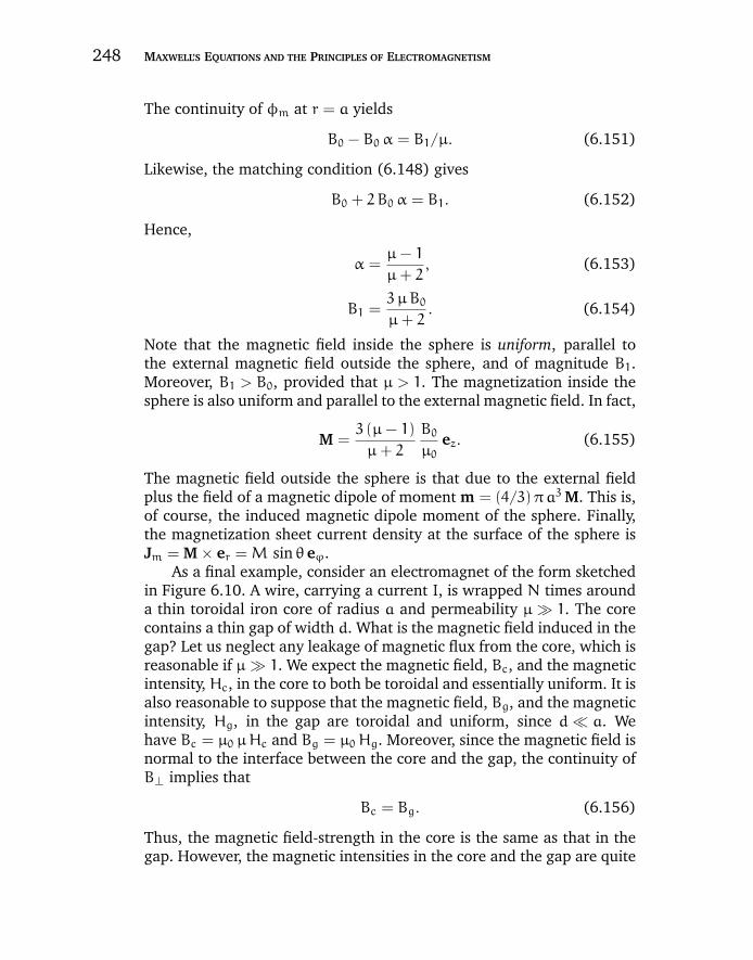
“chapter6” — 2007/12/14 — 12:05 — page 248 — #34
248 MAXWELL’S EQUATIONS AND THE PRINCIPLES OF ELECTROMAGNETISM
The continuity of φm at r = a yields
B0 − B0 α = B1/µ. (6.151)
Likewise, the matching condition (6.148) gives
B0 + 2B0 α = B1. (6.152)
Hence,
α =µ− 1
µ+ 2, (6.153)
B1 =3µB0
µ+ 2. (6.154)
Note that the magnetic field inside the sphere is uniform, parallel tothe external magnetic field outside the sphere, and of magnitude B1.Moreover, B1 > B0, provided that µ > 1. The magnetization inside thesphere is also uniform and parallel to the external magnetic field. In fact,
M =3 (µ− 1)
µ+ 2
B0
µ0ez. (6.155)
The magnetic field outside the sphere is that due to the external fieldplus the field of a magnetic dipole of moment m = (4/3)πa3 M. This is,of course, the induced magnetic dipole moment of the sphere. Finally,the magnetization sheet current density at the surface of the sphere isJm = M × er = M sin θ eϕ.
As a final example, consider an electromagnet of the form sketchedin Figure 6.10. A wire, carrying a current I, is wrapped N times arounda thin toroidal iron core of radius a and permeability µ 1. The corecontains a thin gap of width d. What is the magnetic field induced in thegap? Let us neglect any leakage of magnetic flux from the core, which isreasonable if µ 1. We expect the magnetic field, Bc, and the magneticintensity, Hc, in the core to both be toroidal and essentially uniform. It isalso reasonable to suppose that the magnetic field, Bg, and the magneticintensity, Hg, in the gap are toroidal and uniform, since d a. Wehave Bc = µ0 µHc and Bg = µ0 Hg. Moreover, since the magnetic field isnormal to the interface between the core and the gap, the continuity ofB⊥ implies that
Bc = Bg. (6.156)
Thus, the magnetic field-strength in the core is the same as that in thegap. However, the magnetic intensities in the core and the gap are quite
“chapter6” — 2007/12/14 — 12:05 — page 249 — #35
CHAPTER 6 DIELECTRIC AND MAGNETIC MEDIA 249
iron core
wiregap d
Ia
Figure 6.10: An electromagnet.
different: Hc = Bc/µ0 µ = Bg/µ0 µ = Hg/µ. Integration of Equation(6.128) around the torus yields∮
H · dl =
∫jt · dS = NI. (6.157)
Hence,
(2πa− d)Hc + dHg = NI. (6.158)
It follows that
Bg =Nµ0 I
(2πa− d)/µ+ d. (6.159)
Note that if µ 1 and d 2πa then the magnetic field in the gap isconsiderably larger than that which would be obtained if the core of theelectromagnet were not ferromagnetic.
6.16 MAGNETIC ENERGY
Consider an electrical conductor. Suppose that a battery with an elec-tromotive field E ′ is feeding energy into this conductor. The energy iseither dissipated as heat, or is used to generate a magnetic field. Ohm’slaw inside the conductor gives
jt = σ (E + E ′), (6.160)
“chapter6” — 2007/12/14 — 12:05 — page 250 — #36
250 MAXWELL’S EQUATIONS AND THE PRINCIPLES OF ELECTROMAGNETISM
where jt is the true current density, σ is the conductivity, and E is theinductive electric field. Taking the scalar product with jt, we obtain
E ′ ·jt =j 2tσ
− E · jt. (6.161)
The left-hand side of this equation represents the rate at which the bat-tery does work on the conductor. The first term on the right-hand side isthe rate of ohmic heating inside the conductor. Thus, the remaining termmust represent the rate at which energy is fed into the magnetic field. Ifall fields are quasi-static (i.e., slowly varying) then the displacement cur-rent can be neglected, and the differential form of Ampere’s law reducesto ∇ × H = jt. Substituting this expression into Equation (6.161), andintegrating over all space, we get
∫E ′ ·(∇ × H)d3r =
∫(∇ × H)2
σd3r −
∫E·(∇ × H)d3r. (6.162)
The last term can be integrated by parts using the vector identity
∇·(E × H) ≡ H·(∇ × E) − E·(∇ × H). (6.163)
Gauss’ theorem plus the differential form of Faraday’s law yield∫
E·(∇ × H)d3r = −
∫H·∂B∂td3r −
∫(E × H)·dS. (6.164)
Since E × H falls off at least as fast as 1/r5 in quasi-static electric andmagnetic fields (1/r2 comes from electric monopole fields, and 1/r3 frommagnetic dipole fields), the surface integral in the above expression canbe neglected. Of course, this is not the case for radiation fields, forwhich E and H both fall off like 1/r. Thus, the “quasi-static” constrainteffectively means that the fields vary sufficiently slowly that any radiationfields can be neglected.
The total power expended by the battery can now be written
∫E ′ ·(∇ × H)d3r =
∫(∇ × H)2
σd3r +
∫H·∂B∂td3r. (6.165)
The first term on the right-hand side has already been identified as theenergy loss rate due to ohmic heating, and the second as the rate atwhich energy is fed into the magnetic field. The variation δW in the
“chapter6” — 2007/12/14 — 12:05 — page 251 — #37
CHAPTER 6 DIELECTRIC AND MAGNETIC MEDIA 251
magnetic field energy can therefore be written
δW =
∫H·δBd3r. (6.166)
This result is analogous to the result (6.60) for the variation in the energyof an electrostatic field.
In order to make Equation (6.166) integrable, we must assume afunctional relationship between H and B. For a medium which magne-tizes linearly, the integration can be carried out in an analogous mannerto that used to derive Equation (6.63), to give
W =1
2
∫H·Bd3r. (6.167)
Thus, the magnetostatic energy density inside a linear magnetic materialis given by
U =1
2H· B. (6.168)
Unfortunately, most interesting magnetic materials, such as ferromag-nets, exhibit a nonlinear relationship between H and B. For suchmaterials, Equation (6.166) can only be integrated between definitestates, and the result, in general, depends on the past history of thesample. For ferromagnets, the integral of Equation (6.166) has a finite,non-zero value when B is integrated around a complete magnetizationcycle. This cyclic energy loss is given by
∆W =
∫ ∮H· dBd3r. (6.169)
In other words, the energy expended per unit volume when a magneticmaterial is carried around a magnetization cycle is equal to the areaof its hysteresis loop, as plotted in a graph of B against H. Thus, itis particularly important to ensure that the magnetic materials used toform transformer cores possess hysteresis loops with comparatively smallareas, otherwise the transformers are likely to be extremely lossy.
6.17 EXERCISES
6.1. An infinite slab of dielectric of uniform dielectric constant ε lies between the
planes z = −a and z = a. Suppose that the slab contains free charge of uniform
“chapter6” — 2007/12/14 — 12:05 — page 252 — #38
252 MAXWELL’S EQUATIONS AND THE PRINCIPLES OF ELECTROMAGNETISM
charge density ρf. Find E, D, and P as functions of z. What is the bound charge
sheet density on the two faces of the slab?
6.2. An infinite slab of uncharged dielectric of uniform dielectric constant ε lies
between the planes z = −a and z = a, and is placed in a uniform electric field
E whose field-lines make an angle θ with the z-axis. What is the bound charge
sheet density on the two faces of the slab?
6.3. An uncharged dielectric sphere of radius a, centered on the origin, possesses a
polarization field P = p r, where p is a constant. Find the bound charge density
inside the sphere, and the bound charge sheet density on the surface of the
sphere. Find E and D both inside and outside the sphere.
6.4. An infinite dielectric of dielectric constant ε contains a uniform electric field E0.
Find the electric field inside a needle-shaped cavity running parallel to E0. Find
the field inside a wafer-shaped cavity aligned perpendicular to E0. Neglect end
effects.
6.5. Consider a plane interface between two uniform dielectrics of dielectric constants
ε1 and ε2. A straight electric field-line which passes across the interface is bent
at an angle. Demonstrate that
ε1 tan θ2 = ε2 tan θ1,
where θ1 is the angle the field-line makes with the normal to the interface in
medium 1, etc.
6.6. A charge q lies at the center of an otherwise uncharged dielectric sphere of radius
a and uniform dielectric constant ε. Find D and E throughout space. Find the
bound charge sheet density on the surface of the sphere.
6.7. A cylindrical coaxial cable consists of an inner conductor of radius a, surrounded
by a dielectric sheath of dielectric constant ε1 and outer radius b, surrounded by
a second dielectric sheath of dielectric constant ε2 and outer radius c, surrounded
by an outer conductor. All components of the cable are touching. What is the
capacitance per unit length of the cable?
6.8. A long dielectric cylinder of radius a and uniform dielectric constant ε is placed
in a uniform electric field E0 which runs perpendicular to the axis of the cylinder.
Find the electric field both inside and outside the cylinder. Find the bound charge
sheet density on the surface of the cylinder. Hint: Use separation of variables.
6.9. An electric dipole of moment p = p ez lies at the center of an uncharged dielectric
sphere of radius a and uniform dielectric constant ε. Find D and E throughout
space. Find the bound charge sheet density on the surface of the sphere. Hint:
Use the separation of variables.
6.10. A parallel plate capacitor has plates of area A and spacing d. Half of the region
between the plates is filled with a dielectric of uniform dielectric constant ε1,
“chapter6” — 2007/12/14 — 12:05 — page 253 — #39
CHAPTER 6 DIELECTRIC AND MAGNETIC MEDIA 253
and the other half is filled with a dielectric of uniform dielectric constant ε2.
If the interface between the two dielectric media is a plane parallel to the two
plates, lying half-way between them, what is the capacitance of the capacitor?
If the interface is perpendicular to the two plates, and bisects them, what is the
capacitance of the capacitor?
6.11. Consider a parallel plate capacitor whose plates are of area A and spacing d.
Find the force of attraction per unit area between the plates when:
(a) The region between the plates is empty and the capacitor is connected to a
battery of voltage V .
(b) The capacitor is disconnected from the battery (but remains charged), and
then fully immersed in a dielectric liquid of uniform dielectric constant ε.
(c) The dielectric liquid is replaced by a slab of solid dielectric of uniform dielec-
tric constant ε which fills the region between the plates, but does not touch
the plates.
(d) The uncharged capacitor is fully immersed in a dielectric liquid of uniform
dielectric constant ε, and then charged to a voltage V .
(e) The region between the plates of the uncharged capacitor is filled by a solid
dielectric of uniform dielectric constant ε, which does not touch the plates,
and the capacitor is then charged to a voltage V .
6.12. A parallel plate capacitor has the region between its electrodes completely filled
with a dielectric slab of uniform dielectric constant ε. The plates are of length l,
width w, and spacing d. The capacitor is charged until its plates are at a poten-
tial difference V , and then disconnected. The dielectric slab is then partially
withdrawn in the l dimension until only a length x remains between the plates.
What is the potential difference between the plates? What is the force acting to
pull the slab back toward its initial position? Neglect end effects. Hint: Use an
energy argument to calculate the force.
6.13. A parallel plate capacitor with electrodes of area A, spacing d, which carry
the fixed charges ±Q, is dipped vertically into a large vat of dielectric liquid
of uniform dielectric constant ε and mass density ρm. What height h does the
liquid rise between the plates (relative to the liquid level outside the plates)?
Neglect end effects.
6.14. A solenoid consists of a wire wrapped uniformly around a long, solid, cylindrical
ferromagnetic core of radius a and uniform permeability µ. Suppose that there
are N turns of the wire per unit length. What is the magnetic field-strength
inside the core when a current I flows through the wire? Suppose that the core
is replaced by a cylindrical annulus of the same material. What is the magnetic
field-strength in the cylindrical cavity inside the annulus when a current I flows
through the wire?

“chapter6” — 2007/12/14 — 12:05 — page 254 — #40
254 MAXWELL’S EQUATIONS AND THE PRINCIPLES OF ELECTROMAGNETISM
6.15. A long straight wire carries a current I and is surrounded by a ferromagnetic
co-axial cylindrical annulus of uniform permeability µ, inner radius a, and outer
radius b. Find the magnetic field everywhere. Find the magnetization current
density both within the annulus and on the surfaces of the annulus.
6.16. An infinitely long cylinder of radius a, which is coaxial with the z-axis, has a
uniform magnetization M = M ez. Find the induced magnetic field both inside
and outside the cylinder. Find the magnetization current density on the surface
of the cylinder.
6.17. A very large piece of magnetic material of constant permeability µ contains
a uniform magnetic field B0. Find the magnetic field inside a needle-shaped
cavity running parallel to B0. Find the field inside a wafer-shaped cavity aligned
perpendicular to B0. Neglect end effects.
6.18. A spherical annulus of magnetic material of inner radius a, outer radius b, and
uniform permeability µ is placed in the uniform magnetic field B = B0 ez. Find
the magnetic scalar potential everywhere. What is the magnetic field inside the
shell? Hint: Use the separation of variables.
6.19. A long ferromagnetic cylinder of radius a and uniform permeability µ is placed
in a uniform magnetic field B0 which runs perpendicular to the axis of the
cylinder. Find the magnetic field both inside and outside the cylinder. Find the
magnetization current on the surface of the cylinder. Hint: Use separation of
variables.
6.20. A magnetic dipole of moment m = m ez lies at the center of a ferromagnetic
sphere of radius a and uniform permeability µ. Find H and B throughout space.
Find the magnetization current density on the surface of the sphere. Hint: Use
the separation of variables.
6.21. A magnet consists of a thin ring of magnetic material of radius a containing a
narrow gap of width d, where d a (i.e., the magnet has the same shape as the
core of the electromagnet shown in Figure 6.10). The magnetic material pos-
sesses a uniform permanent magnetization M = M eϕ, where eϕ is a unit vector
which runs toroidally around the ring. What is the strength of the magnetic field
in the gap? If A is the cross-sectional area of the ring, how much magnetostatic
energy does the magnet possess? Neglect field leakage.
6.22. Suppose that half of the permanently magnetized material making up the ring
in the previous question is replaced by material of uniform permeability µ. What
is the magnetic field-strength in the gap? How much magnetostatic energy does
the magnet possess? Neglect field leakage.
“chapter7” — 2007/12/14 — 12:08 — page 255 — #1
C h a p t e r 7 MAGNETICINDUCTION
7.1 INTRODUCTION
In this chapter, we shall use Maxwell’s equations to investigate magneticinduction and related phenomena.
7.2 INDUCTANCE
We have already learned about the concepts of voltage, resistance, andcapacitance. Let us now investigate the concept of inductance. Electricalengineers like to reduce all pieces of electrical circuitary to an equivalentcircuit consisting of pure voltage sources, pure inductors, pure capaci-tors, and pure resistors. Hence, once we understand inductors, we shallbe ready to apply the laws of electromagnetism to general electricalcircuits.
Consider two stationary loops of wire, labeled 1 and 2—see Fig-ure 7.1. Let us run a steady current I1 around the first loop to producea magnetic field B1. Some of the field-lines of B1 will pass through thesecond loop. Let Φ2 be the flux of B1 through loop 2,
Φ2 =
∫loop 2
B1 · dS2, (7.1)
where dS2 is a surface element of loop 2. This flux is generally quitedifficult to calculate exactly (unless the two loops have a particularlysimple geometry). However, we can infer from the Biot-Savart law,
B1(r) =µ0 I1
4π
∮loop 1
dl1 × (r − r1)|r − r1|3
, (7.2)
that the magnitude of B1 is proportional to the current I1. This is ulti-mately a consequence of the linearity of Maxwell’s equations. Here, dl1is a line element of loop 1 located at position vector r1. It follows that
255
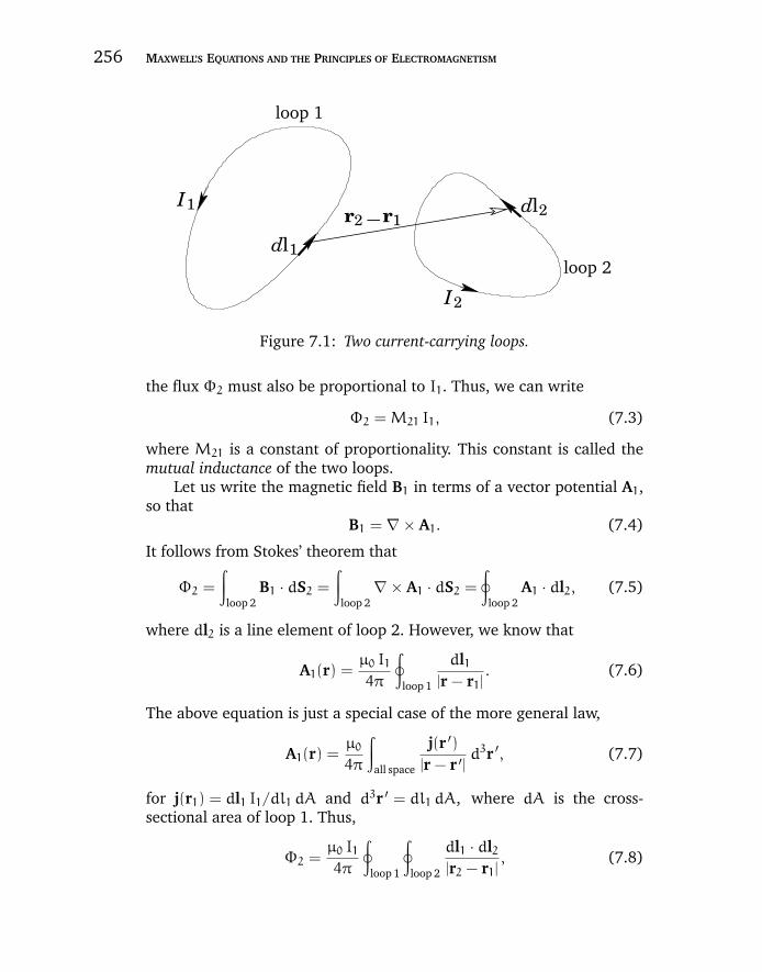
“chapter7” — 2007/12/14 — 12:08 — page 256 — #2
256 MAXWELL’S EQUATIONS AND THE PRINCIPLES OF ELECTROMAGNETISM
loop 2
dl2
loop 1
dl1
r2r1I1
I2
Figure 7.1: Two current-carrying loops.
the flux Φ2 must also be proportional to I1. Thus, we can write
Φ2 = M21 I1, (7.3)
where M21 is a constant of proportionality. This constant is called themutual inductance of the two loops.
Let us write the magnetic field B1 in terms of a vector potential A1,so that
B1 = ∇ × A1. (7.4)
It follows from Stokes’ theorem that
Φ2 =
∫loop 2
B1 · dS2 =
∫loop 2
∇ × A1 · dS2 =
∮loop 2
A1 · dl2, (7.5)
where dl2 is a line element of loop 2. However, we know that
A1(r) =µ0 I1
4π
∮loop 1
dl1|r − r1|
. (7.6)
The above equation is just a special case of the more general law,
A1(r) =µ0
4π
∫all space
j(r ′)|r − r ′|
d3r ′, (7.7)
for j(r1) = dl1 I1/dl1 dA and d3r ′ = dl1 dA, where dA is the cross-sectional area of loop 1. Thus,
Φ2 =µ0 I1
4π
∮loop 1
∮loop 2
dl1 · dl2|r2 − r1|
, (7.8)

“chapter7” — 2007/12/14 — 12:08 — page 257 — #3
CHAPTER 7 MAGNETIC INDUCTION 257
where r2 is the position vector of the line element dl2 of loop 2, whichimplies that
M21 =µ0
4π
∮loop 1
∮loop 2
dl1 · dl2|r2 − r1|
. (7.9)
In fact, mutual inductances are rarely worked out using the above for-mula, because it is usually much too difficult. However, this expression—which is known as the Neumann formula—tells us two important things.Firstly, the mutual inductance of two current loops is a purely geometricquantity, having to do with the sizes, shapes, and relative orientationsof the loops. Secondly, the integral is unchanged if we switch the rolesof loops 1 and 2. In other words,
M21 = M12. (7.10)
Hence, we can drop the subscripts, and just call both these quantitiesM.This is a rather surprising result. It implies that no matter what the shapesand relative positions of the two loops, the magnetic flux through loop 2when we run a current I around loop 1 is exactly the same as the fluxthrough loop 1 when we run the same current around loop 2.
We have seen that a current I flowing around some wire loop, 1,generates a magnetic flux linking some other loop, 2. However, flux isalso generated through the first loop. As before, the magnetic field, and,therefore, the flux, Φ, is proportional to the current, so we can write
Φ = L I. (7.11)
The constant of proportionality L is called the self-inductance. Like M itonly depends on the geometry of the loop.
Inductance is measured in SI units called henries (H): 1 henry is 1volt-second per ampere. The henry, like the farad, is a rather unwieldyunit, since inductors in electrical circuits typically have inductances oforder one micro-henry.
7.3 SELF-INDUCTANCE
Consider a long, uniformly wound, cylindrical solenoid of length l, andradius r, which has N turns per unit length, and carries a current I. Thelongitudinal (i.e., directed along the axis of the solenoid) magnetic field
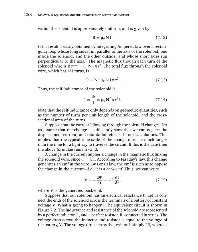
“chapter7” — 2007/12/14 — 12:08 — page 258 — #4
258 MAXWELL’S EQUATIONS AND THE PRINCIPLES OF ELECTROMAGNETISM
within the solenoid is approximately uniform, and is given by
B = µ0 N I. (7.12)
(This result is easily obtained by integrating Ampere’s law over a rectan-gular loop whose long sides run parallel to the axis of the solenoid, oneinside the solenoid, and the other outside, and whose short sides runperpendicular to the axis.) The magnetic flux though each turn of thesolenoid wire is Bπ r2 = µ0 N Iπ r
2. The total flux through the solenoidwire, which has Nl turns, is
Φ = Nlµ0 N Iπ r2. (7.13)
Thus, the self-inductance of the solenoid is
L =Φ
I= µ0 N
2 π r2 l. (7.14)
Note that the self-inductance only depends on geometric quantities, suchas the number of turns per unit length of the solenoid, and the cross-sectional area of the turns.
Suppose that the current I flowing through the solenoid changes. Letus assume that the change is sufficiently slow that we can neglect thedisplacement current, and retardation effects, in our calculations. Thisimplies that the typical time-scale of the change must be much longerthan the time for a light-ray to traverse the circuit. If this is the case thenthe above formulae remain valid.
A change in the current implies a change in the magnetic flux linkingthe solenoid wire, sinceΦ = L I. According to Faraday’s law, this changegenerates an emf in the wire. By Lenz’s law, the emf is such as to opposethe change in the current—i.e., it is a back-emf. Thus, we can write
V = −dΦ
dt= −L
dI
dt, (7.15)
where V is the generated back-emf.Suppose that our solenoid has an electrical resistance R. Let us con-
nect the ends of the solenoid across the terminals of a battery of constantvoltage V. What is going to happen? The equivalent circuit is shown inFigure 7.2. The inductance and resistance of the solenoid are representedby a perfect inductor, L, and a perfect resistor, R, connected in series. Thevoltage drop across the inductor and resistor is equal to the voltage ofthe battery, V. The voltage drop across the resistor is simply I R, whereas
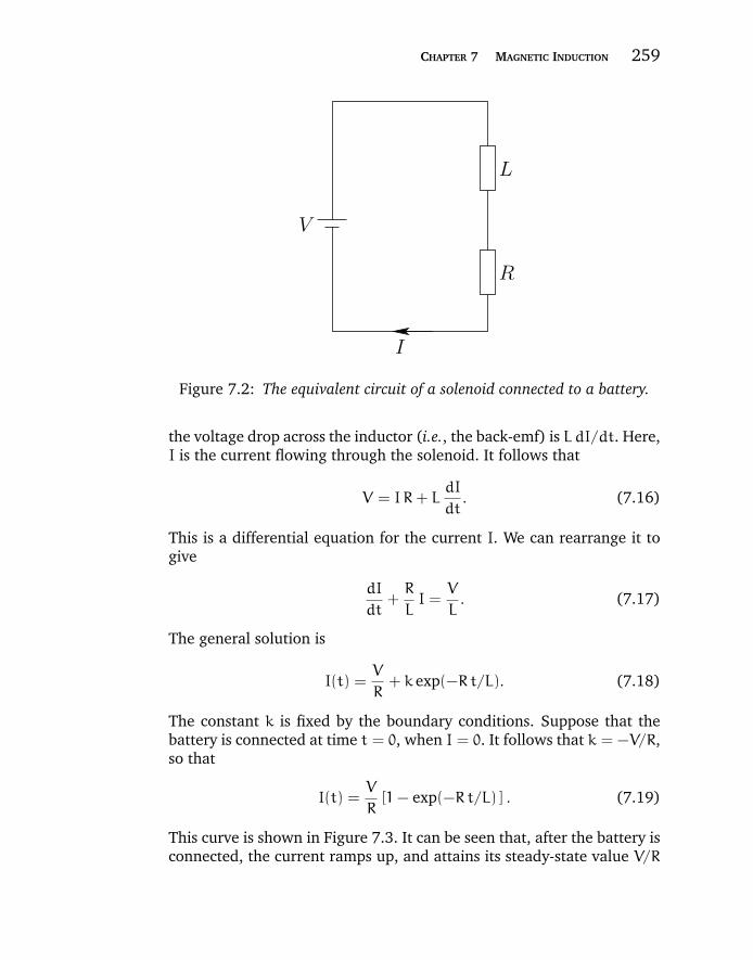
“chapter7” — 2007/12/14 — 12:08 — page 259 — #5
CHAPTER 7 MAGNETIC INDUCTION 259
R
V
I
L
Figure 7.2: The equivalent circuit of a solenoid connected to a battery.
the voltage drop across the inductor (i.e., the back-emf) is LdI/dt. Here,I is the current flowing through the solenoid. It follows that
V = I R+ LdI
dt. (7.16)
This is a differential equation for the current I. We can rearrange it togive
dI
dt+R
LI =
V
L. (7.17)
The general solution is
I(t) =V
R+ k exp(−R t/L). (7.18)
The constant k is fixed by the boundary conditions. Suppose that thebattery is connected at time t = 0, when I = 0. It follows that k = −V/R,so that
I(t) =V
R[1− exp(−R t/L) ] . (7.19)
This curve is shown in Figure 7.3. It can be seen that, after the battery isconnected, the current ramps up, and attains its steady-state value V/R
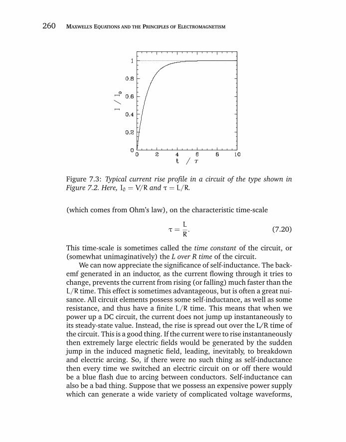
“chapter7” — 2007/12/14 — 12:08 — page 260 — #6
260 MAXWELL’S EQUATIONS AND THE PRINCIPLES OF ELECTROMAGNETISM
Figure 7.3: Typical current rise profile in a circuit of the type shown inFigure 7.2. Here, I0 = V/R and τ = L/R.
(which comes from Ohm’s law), on the characteristic time-scale
τ =L
R. (7.20)
This time-scale is sometimes called the time constant of the circuit, or(somewhat unimaginatively) the L over R time of the circuit.
We can now appreciate the significance of self-inductance. The back-emf generated in an inductor, as the current flowing through it tries tochange, prevents the current from rising (or falling) much faster than theL/R time. This effect is sometimes advantageous, but is often a great nui-sance. All circuit elements possess some self-inductance, as well as someresistance, and thus have a finite L/R time. This means that when wepower up a DC circuit, the current does not jump up instantaneously toits steady-state value. Instead, the rise is spread out over the L/R time ofthe circuit. This is a good thing. If the current were to rise instantaneouslythen extremely large electric fields would be generated by the suddenjump in the induced magnetic field, leading, inevitably, to breakdownand electric arcing. So, if there were no such thing as self-inductancethen every time we switched an electric circuit on or off there wouldbe a blue flash due to arcing between conductors. Self-inductance canalso be a bad thing. Suppose that we possess an expensive power supplywhich can generate a wide variety of complicated voltage waveforms,
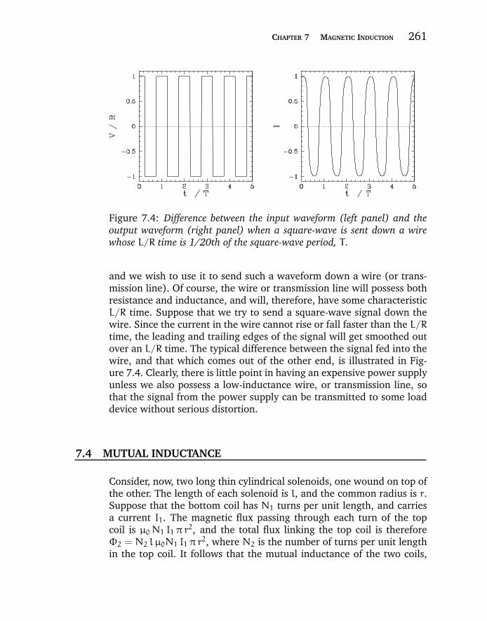
“chapter7” — 2007/12/14 — 12:08 — page 261 — #7
CHAPTER 7 MAGNETIC INDUCTION 261
Figure 7.4: Difference between the input waveform (left panel) and theoutput waveform (right panel) when a square-wave is sent down a wirewhose L/R time is 1/20th of the square-wave period, T .
and we wish to use it to send such a waveform down a wire (or trans-mission line). Of course, the wire or transmission line will possess bothresistance and inductance, and will, therefore, have some characteristicL/R time. Suppose that we try to send a square-wave signal down thewire. Since the current in the wire cannot rise or fall faster than the L/Rtime, the leading and trailing edges of the signal will get smoothed outover an L/R time. The typical difference between the signal fed into thewire, and that which comes out of the other end, is illustrated in Fig-ure 7.4. Clearly, there is little point in having an expensive power supplyunless we also possess a low-inductance wire, or transmission line, sothat the signal from the power supply can be transmitted to some loaddevice without serious distortion.
7.4 MUTUAL INDUCTANCE
Consider, now, two long thin cylindrical solenoids, one wound on top ofthe other. The length of each solenoid is l, and the common radius is r.Suppose that the bottom coil has N1 turns per unit length, and carriesa current I1. The magnetic flux passing through each turn of the topcoil is µ0 N1 I1 π r2, and the total flux linking the top coil is thereforeΦ2 = N2 l µ0N1 I1 π r
2, where N2 is the number of turns per unit lengthin the top coil. It follows that the mutual inductance of the two coils,
“chapter7” — 2007/12/14 — 12:08 — page 262 — #8
262 MAXWELL’S EQUATIONS AND THE PRINCIPLES OF ELECTROMAGNETISM
defined Φ2 = MI1, is given by
M = µ0 N1 N2 π r2 l. (7.21)
Recall that the self-inductance of the bottom coil is
L1 = µ0 N21 π r
2 l, (7.22)
and that of the top coil is
L2 = µ0 N22 π r
2 l. (7.23)
Hence, the mutual inductance can be written
M =√L1 L2. (7.24)
Note that this result depends on the assumption that all of the magneticflux produced by one coil passes through the other coil. In reality, someof the flux leaks out, so that the mutual inductance is somewhat lessthan that given in the above formula. We can write
M = k√L1 L2, (7.25)
where the dimensionless constant k is called the coefficient of coupling,and lies in the range 0 ≤ k ≤ 1.
Suppose that the two coils have resistances R1 and R2. If the bot-tom coil has an instantaneous current I1 flowing through it, and a totalvoltage drop V1, then the voltage drop due to its resistance is I1 R1. Thevoltage drop due to the back-emf generated by the self-inductance of thecoil is L1 dI1/dt. There is also a back-emf due to inductive coupling withthe top coil. We know that the flux through the bottom coil due to theinstantaneous current I2 flowing in the top coil is
Φ1 = MI2. (7.26)
Thus, by Faraday’s law and Lenz’s law, the back-emf induced in thebottom coil is
V = −MdI2
dt. (7.27)
The voltage drop across the bottom coil due to its mutual inductancewith the top coil is minus this expression. Thus, the circuit equation forthe bottom coil is
V1 = R1 I1 + L1dI1
dt+M
dI2
dt. (7.28)
“chapter7” — 2007/12/14 — 12:08 — page 263 — #9
CHAPTER 7 MAGNETIC INDUCTION 263
Likewise, the circuit equation for the top coil is
V2 = R2 I2 + L2dI2
dt+M
dI1
dt. (7.29)
Here, V2 is the total voltage drop across the top coil.Suppose that we suddenly connect a battery of constant voltage V1
to the bottom coil, at time t = 0. The top coil is assumed to be open-circuited, or connected to a voltmeter of very high internal resistance, sothat I2 = 0. What is the voltage generated in the top coil? Since I2 = 0,the circuit equation for the bottom coil is
V1 = R1 I1 + L1dI1
dt, (7.30)
where V1 is constant, and I1(t = 0) = 0. We have already seen thesolution to this equation:
I1 =V1
R1[1− exp(−R1 t/L1)] . (7.31)
The circuit equation for the top coil is
V2 = MdI1
dt, (7.32)
giving
V2 = V1M
L1exp(−R1 t/L1). (7.33)
It follows from Equation (7.25) that
V2 = V1 k
√L2
L1exp(−R1 t/L1). (7.34)
Since L1/L2 = N21 /N
22 , we obtain
V2 = V1 kN2
N1exp(−R1 t/L1). (7.35)
Note that V2(t) is discontinuous at t = 0. This is not a problem, sincethe resistance of the top circuit is infinite, so there is no discontinuityin the current (and, hence, in the magnetic field). But, what about thedisplacement current, which is proportional to ∂E/∂t? Surely, this isdiscontinuous at t = 0 (which is clearly unphysical)? The crucial point,
“chapter7” — 2007/12/14 — 12:08 — page 264 — #10
264 MAXWELL’S EQUATIONS AND THE PRINCIPLES OF ELECTROMAGNETISM
here, is that we have specifically neglected the displacement current inall of our previous analysis, so it does not make much sense to startworrying about it now. If we had retained the displacement current inour calculations then we would have found that the voltage in the topcircuit jumps up, at t = 0, on a time-scale similar to the light traversetime across the circuit (i.e., the jump is instantaneous, to all intents andpurposes, but the displacement current remains finite).
Now,
V2(t = 0)
V1= k
N2
N1, (7.36)
so if N2 N1 then the voltage in the bottom circuit is considerablyamplified in the top circuit. This effect is the basis for old-fashioned carignition systems. A large voltage spike is induced in a secondary circuit(connected to a coil with very many turns) whenever the current in aprimary circuit (connected to a coil with not so many turns) is eitherswitched on or off. The primary circuit is connected to the car battery(whose voltage is typically 12 volts). The switching is done by a set ofpoints, which are mechanically opened and closed as the engine turns.The large voltage spike induced in the secondary circuit, as the pointsare either opened or closed, causes a spark to jump across a gap in thiscircuit. This spark ignites a petrol/air mixture in one of the cylinders. Wemight think that the optimum configuration is to have only one turn inthe primary circuit, and lots of turns in the secondary circuit, so that theratio N2/N1 is made as large as possible. However, this is not the case.Most of the magnetic flux generated by a single turn primary coil is likelyto miss the secondary coil altogether. This means that the coefficient ofcoupling k is small, which reduces the voltage induced in the secondarycircuit. Thus, we need a reasonable number of turns in the primary coilin order to localize the induced magnetic flux, so that it links effectivelywith the secondary coil.
7.5 MAGNETIC ENERGY
Suppose that, at t = 0, a coil of inductance, L, and resistance R, isconnected across the terminals of a battery of voltage V. The circuitequation is
V = LdI
dt+ R I. (7.37)

“chapter7” — 2007/12/14 — 12:08 — page 265 — #11
CHAPTER 7 MAGNETIC INDUCTION 265
Now, the power output of the battery is V I. [Every charge q that goesaround the circuit falls through a potential difference qV. In order toraise it back to the starting potential, so that it can perform anothercircuit, the battery must do work qV. The work done per unit time (i.e.,the power) is nqV, where n is the number of charges per unit timepassing a given point on the circuit. But, I = nq, so the power output isV I.] Thus, the net work done by the battery in raising the current in thecircuit from zero at time t = 0 to IT at time t = T is
W =
∫ T0
V I dt. (7.38)
Using the circuit equation (7.37), we obtain
W = L
∫ T0
IdI
dtdt+ R
∫ T0
I2 dt, (7.39)
giving
W =1
2L I 2T + R
∫ T0
I2 dt. (7.40)
The second term on the right-hand side of the above equation representsthe irreversible conversion of electrical energy into heat energy by theresistor. The first term is the amount of energy stored in the inductor attime T . This energy can be recovered after the inductor is disconnectedfrom the battery. Suppose that the battery is disconnected at time T . Thecircuit equation is now
0 = LdI
dt+ RI, (7.41)
giving
I = IT exp[−R
L(t− T)
], (7.42)
where we have made use of the boundary condition I(T) = IT . Thus, thecurrent decays away exponentially. The energy stored in the inductor isdissipated as heat in the resistor. The total heat energy appearing in theresistor after the battery is disconnected is∫
∞
T
I2 R dt =1
2L I 2T , (7.43)
where use has been made of Equation (7.42). Thus, the heat energyappearing in the resistor is equal to the energy stored in the inductor.
“chapter7” — 2007/12/14 — 12:08 — page 266 — #12
266 MAXWELL’S EQUATIONS AND THE PRINCIPLES OF ELECTROMAGNETISM
This energy is actually stored in the magnetic field generated aroundthe inductor.
Consider, again, our circuit with two coils wound on top of oneanother. Suppose that each coil is connected to its own battery. Thecircuit equations are thus
V1 = R1 I1 + L1dI1
dt+M
dI2
dt,
V2 = R2 I2 + L2dI2
dt+M
dI1
dt, (7.44)
where V1 is the voltage of the battery in the first circuit, etc. The net workdone by the two batteries in increasing the currents in the two circuits,from zero at time 0, to I1 and I2 at time T , respectively, is
W =
∫ T0
(V1 I1 + V2 I2)dt
=
∫ T0
(R1 I21 + R2 I
22 )dt+
1
2L1 I
21 +
1
2L2 I
22
+M
∫ T0
(I1dI2
dt+ I2
dI1
dt
)dt. (7.45)
Thus,
W =
∫ T0
(R1 I21 + R2 I
22 )dt
+1
2L1 I
21 +
1
2L2 I
22 +MI1 I2. (7.46)
Clearly, the total magnetic energy stored in the two coils is
WB =1
2L1 I
21 +
1
2L2 I
22 +MI1 I2. (7.47)
Note that the mutual inductance term increases the stored magneticenergy if I1 and I2 are of the same sign—i.e., if the currents in the twocoils flow in the same direction, so that they generate magnetic fieldswhich reinforce one another. Conversely, the mutual inductance termdecreases the stored magnetic energy if I1 and I2 are of the oppositesign. However, the total stored energy can never be negative, otherwisethe coils would constitute a power source (a negative stored energy isequivalent to a positive generated energy). Thus,
1
2L1 I
21 +
1
2L2 I
22 +MI1 I2 ≥ 0, (7.48)
“chapter7” — 2007/12/14 — 12:08 — page 267 — #13
CHAPTER 7 MAGNETIC INDUCTION 267
which can be written
1
2
(√L1 I1 +
√L2 I2
)2− I1 I2(
√L1 L2 −M) ≥ 0, (7.49)
assuming that I1 I2 < 0. It follows that
M ≤√L1 L2. (7.50)
The equality sign corresponds to the situation in which all of the magneticflux generated by one coil passes through the other. If some of the fluxmisses then the inequality sign is appropriate. In fact, the above formulais valid for any two inductively coupled circuits, and effectively sets anupper limit on their mutual inductance.
We intimated previously that the energy stored in an inductor isactually stored in the surrounding magnetic field. Let us now obtainan explicit formula for the energy stored in a magnetic field. Consideran ideal cylindrical solenoid. The energy stored in the solenoid when acurrent I flows through it is
W =1
2L I2, (7.51)
where L is the self-inductance. We know that
L = µ0 N2 π r2 l, (7.52)
where N is the number of turns per unit length of the solenoid, rthe radius, and l the length. The magnetic field inside the solenoid isapproximately uniform, with magnitude
B = µ0 N I, (7.53)
and is approximately zero outside the solenoid. Equation (7.51) can berewritten
W =B2
2µ0V, (7.54)
where V = π r2 l is the volume of the solenoid. The above formulastrongly suggests that a magnetic field possesses an energy density
U =B2
2µ0. (7.55)
Let us now examine a more general proof of the above formula.Consider a system of N circuits (labeled i = 1 to N), each carrying
“chapter7” — 2007/12/14 — 12:08 — page 268 — #14
268 MAXWELL’S EQUATIONS AND THE PRINCIPLES OF ELECTROMAGNETISM
a current Ii. The magnetic flux through the ith circuit is written [cf.,Equation (7.5)]
Φi =
∫B · dSi =
∮A · dli, (7.56)
where B = ∇ × A, and dSi and dli denote a surface element and a lineelement of this circuit, respectively. The back-emf induced in the ithcircuit follows from Faraday’s law:
Vi = −dΦi
dt. (7.57)
The rate of work of the battery which maintains the current Ii in the ithcircuit against this back-emf is
Pi = IidΦi
dt. (7.58)
Thus, the total work required to raise the currents in theN circuits fromzero at time 0, to I0 i at time T , is
W =
N∑i=1
∫ T0
IidΦi
dtdt. (7.59)
The above expression for the work done is, of course, equivalent to thetotal energy stored in the magnetic field surrounding the various circuits.This energy is independent of the manner in which the currents are setup. Suppose, for the sake of simplicity, that the currents are ramped uplinearly, so that
Ii = I0 it
T. (7.60)
The fluxes are proportional to the currents, so they must also ramp uplinearly: i.e.,
Φi = Φ0 it
T. (7.61)
It follows that
W =
N∑i=1
∫ T0
I0 i Φ0 it
T2dt, (7.62)
“chapter7” — 2007/12/14 — 12:08 — page 269 — #15
CHAPTER 7 MAGNETIC INDUCTION 269
giving
W =1
2
N∑i=1
I0 i Φ0 i. (7.63)
So, if instantaneous currents Ii flow in the the N circuits, which linkinstantaneous fluxes Φi, then the instantaneous stored energy is
W =1
2
N∑i=1
Ii Φi. (7.64)
Equations (7.56) and (7.64) imply that
W =1
2
N∑i=1
Ii
∮A · dli. (7.65)
It is convenient, at this stage, to replace ourN line currents byN currentdistributions of small, but finite, cross-sectional area. Equation (7.65)transforms to
W =1
2
∫V
A · jdV, (7.66)
where V is a volume which contains all of the circuits. Note that foran element of the ith circuit, j = Ii dli/dli Ai and dV = dli Ai, whereAi is the cross-sectional area of the circuit. Now, µ0 j = ∇ × B (we areneglecting the displacement current in this calculation), so
W =1
2µ0
∫V
A · ∇ × BdV. (7.67)
According to vector field theory,
∇ · (A × B) ≡ B · ∇ × A − A · ∇ × B, (7.68)
which implies that
W =1
2µ0
∫V
[−∇ · (A × B) + B · ∇ × A] dV. (7.69)
Using Gauss’ theorem, and B = ∇ × A, we obtain
W = −1
2µ0
∮S
A × B · dS +1
2µ0
∫V
B2 dV, (7.70)
where S is the bounding surface of some volume V. Let us take this sur-face to infinity. It is easily demonstrated that the magnetic field generated
“chapter7” — 2007/12/14 — 12:08 — page 270 — #16
270 MAXWELL’S EQUATIONS AND THE PRINCIPLES OF ELECTROMAGNETISM
by a current loop falls of like r−3 at large distances. The vector potentialfalls off like r−2. However, the area of surface S only increases like r2. Itfollows that the surface integral is negligible in the limit r → ∞. Thus,the above expression reduces to
W =
∫B2
2µ0dV, (7.71)
where the integral is over all space. Since this expression is valid forany magnetic field whatsoever, we can safely conclude that the energydensity of a general magnetic field generated by a system of electricalcircuits is given by
U =B2
2µ0. (7.72)
Note, that the above expression is consistent with Equation (6.168)which we previously obtained during our investigation of magneticmedia.
7.6 ALTERNATING CURRENT CIRCUITS
Alternating current (AC) circuits are made up of voltage sources andthree different types of passive elements: i.e., resistors, inductors, andcapacitors. Resistors satisfy Ohm’s law,
V = I R, (7.73)
where R is the resistance, I the current flowing through the resistor,and V the voltage drop across the resistor (in the direction in which thecurrent flows). Inductors satisfy
V = LdI
dt, (7.74)
where L is the inductance. Finally, capacitors obey
V =q
C=
∫ t0
I dt
/C, (7.75)
where C is the capacitance, q is the charge stored on the plate withthe most positive potential, and I = 0 for t < 0. Note that any passivecomponent of a real electrical circuit can always be represented as acombination of ideal resistors, inductors, and capacitors.
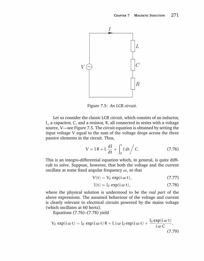
“chapter7” — 2007/12/14 — 12:08 — page 271 — #17
CHAPTER 7 MAGNETIC INDUCTION 271
L
C
R
V
I
Figure 7.5: An LCR circuit.
Let us consider the classic LCR circuit, which consists of an inductor,L, a capacitor, C, and a resistor, R, all connected in series with a voltagesource, V—see Figure 7.5. The circuit equation is obtained by setting theinput voltage V equal to the sum of the voltage drops across the threepassive elements in the circuit. Thus,
V = I R+ LdI
dt+
∫ t0
I dt
/C. (7.76)
This is an integro-differential equation which, in general, is quite diffi-cult to solve. Suppose, however, that both the voltage and the currentoscillate at some fixed angular frequency ω, so that
V(t) = V0 exp(iωt), (7.77)
I(t) = I0 exp(iωt), (7.78)
where the physical solution is understood to be the real part of theabove expressions. The assumed behaviour of the voltage and currentis clearly relevant to electrical circuits powered by the mains voltage(which oscillates at 60 hertz).
Equations (7.76)–(7.78) yield
V0 exp(iωt) = I0 exp(iωt)R+ L iωI0 exp(iωt) +I0 exp(iωt)
iωC,
(7.79)
“chapter7” — 2007/12/14 — 12:08 — page 272 — #18
272 MAXWELL’S EQUATIONS AND THE PRINCIPLES OF ELECTROMAGNETISM
giving
V0 = I0
(iωL+
1
iωC+ R
). (7.80)
It is helpful to define the impedance of the circuit:
Z =V
I= iωL+
1
iωC+ R. (7.81)
Impedance is a generalization of the concept of resistance. In general,the impedance of an AC circuit is a complex quantity.
The average power output of the voltage source is
P = 〈V(t) I(t)〉, (7.82)
where the average is taken over one period of the oscillation. Let us, firstof all, calculate the power using real (rather than complex) voltages andcurrents. We can write
V(t) = |V0| cos(ωt), (7.83)
I(t) = |I0| cos(ωt− θ), (7.84)
where θ is the phase-lag of the current with respect to the voltage. Itfollows that
P = |V0| |I0|
∫ωt=2πωt=0
cos(ωt) cos(ωt− θ)d(ωt)
2π(7.85)
= |V0| |I0|
∫ωt=2πωt=0
cos(ωt) [cos(ωt) cos θ+ sin(ωt) sin θ]d(ωt)
2π,
giving
P =1
2|V0| |I0| cos θ, (7.86)
since 〈cos(ωt) sin(ωt)〉 = 0 and 〈cos(ωt) cos(ωt)〉 = 1/2. In complexrepresentation, the voltage and the current are written
V(t) = |V0| exp(iωt), (7.87)
I(t) = |I0| exp[i (ωt− θ)]. (7.88)
Now,
1
2(V I∗ + V∗ I) = |V0| |I0| cos θ. (7.89)
“chapter7” — 2007/12/14 — 12:08 — page 273 — #19
CHAPTER 7 MAGNETIC INDUCTION 273
It follows that
P =1
4(V I∗ + V∗ I) =
1
2Re(V I∗). (7.90)
Making use of Equation (7.81), we find that
P =1
2Re(Z) |I|2 =
1
2
Re(Z) |V |2
|Z|2. (7.91)
Note that power dissipation is associated with the real part of theimpedance. For the special case of an LCR circuit,
P =1
2R |I0|
2. (7.92)
We conclude that only the resistor dissipates energy in this circuit. Theinductor and the capacitor both store energy, but they eventually returnit to the circuit without dissipation.
According to Equation (7.81), the amplitude of the current whichflows in an LCR circuit for a given amplitude of the input voltage isgiven by
|I0| =|V0|
|Z|=
|V0|√(ωL− 1/ωC)2 + R2
. (7.93)
As can be seen from Figure 7.6, the response of the circuit is reso-nant, peaking at ω = 1/
√LC, and reaching 1/
√2 of the peak value
at ω = 1/√LC± R/(2 L) (assuming that R √
L/C). For this reason,LCR circuits are used in analog radio tuners to filter out signals whosefrequencies fall outside a given band.
The phase-lag of the current with respect to the voltage is given by
θ = arg(Z) = tan−1
(ωL− 1/ωC
R
). (7.94)
As can be seen from Figure 7.6, the phase-lag varies from −π/2 forfrequencies significantly below the resonant frequency, to zero at theresonant frequency (ω = 1/
√LC), to π/2 for frequencies significantly
above the resonant frequency.It is clear that in conventional AC circuits the circuit equation reduces
to a simple algebraic equation, and that the behavior of the circuit issummed up by the complex impedance, Z. The real part of Z tells usthe power dissipated in the circuit, the magnitude of Z gives the ratio ofthe peak current to the peak voltage, and the argument of Z gives thephase-lag of the current with respect to the voltage.

“chapter7” — 2007/12/14 — 12:08 — page 274 — #20
274 MAXWELL’S EQUATIONS AND THE PRINCIPLES OF ELECTROMAGNETISM
Figure 7.6: The characteristics of an LCR circuit. The left-hand andright-hand panes show the amplitude and phase-lag of the current versusfrequency, respectively. Here, ωc = 1/
√LC and Z0 =
√L/C. The solid,
short-dashed, long-dashed, and dot-dashed curves correspond to R/Z0 = 1,1/2, 1/4, and 1/8, respectively.
7.7 TRANSMISSION LINES
The central assumption made in the analysis of conventional AC circuitsis that the voltage (and, hence, the current) has the same phase through-out the circuit. Unfortunately, if the circuit is sufficiently large, or thefrequency of oscillation, ω, is sufficiently high, then this assumptionbecomes invalid. The assumption of a constant phase throughout thecircuit is reasonable if the wavelength of the oscillation, λ = 2π c/ω, ismuch larger than the dimensions of the circuit. (Here, we assume thatsignals propagate around electrical circuits at about the velocity of light.This assumption will be justified later on.) This is generally not the casein electrical circuits which are associated with communication. The fre-quencies in such circuits tend to be very high, and the dimensions are,almost by definition, large. For instance, leased telephone lines (the typeto which computers are connected) run at 56 kHz. The correspondingwavelength is about 5 km, so the constant-phase approximation clearlybreaks down for long-distance calls. Computer networks generally runat about 100 MHz, corresponding to λ ∼ 3 m. Thus, the constant-phaseapproximation also breaks down for most computer networks, since suchnetworks are generally significantly larger than 3 m. It turns out that weneed a special sort of wire, called a transmission line, to propagate signalsaround circuits whose dimensions greatly exceed the wavelength, λ. Letus investigate transmission lines.
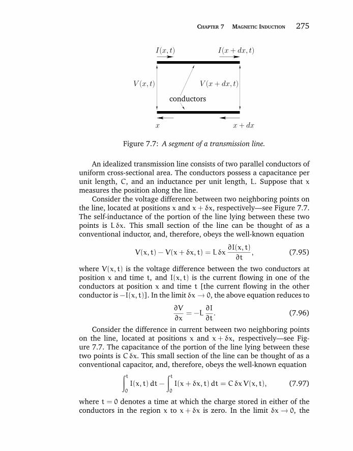
“chapter7” — 2007/12/14 — 12:08 — page 275 — #21
CHAPTER 7 MAGNETIC INDUCTION 275
V (x + dx, t)V (x, t)
I(x, t) I(x + dx, t)
conductors
x x + dx
Figure 7.7: A segment of a transmission line.
An idealized transmission line consists of two parallel conductors ofuniform cross-sectional area. The conductors possess a capacitance perunit length, C, and an inductance per unit length, L. Suppose that xmeasures the position along the line.
Consider the voltage difference between two neighboring points onthe line, located at positions x and x+ δx, respectively—see Figure 7.7.The self-inductance of the portion of the line lying between these twopoints is L δx. This small section of the line can be thought of as aconventional inductor, and, therefore, obeys the well-known equation
V(x, t) − V(x+ δx, t) = L δx∂I(x, t)
∂t, (7.95)
where V(x, t) is the voltage difference between the two conductors atposition x and time t, and I(x, t) is the current flowing in one of theconductors at position x and time t [the current flowing in the otherconductor is −I(x, t)]. In the limit δx → 0, the above equation reduces to
∂V
∂x= −L
∂I
∂t. (7.96)
Consider the difference in current between two neighboring pointson the line, located at positions x and x+ δx, respectively—see Fig-ure 7.7. The capacitance of the portion of the line lying between thesetwo points is Cδx. This small section of the line can be thought of as aconventional capacitor, and, therefore, obeys the well-known equation∫ t
0
I(x, t)dt−
∫ t0
I(x+ δx, t)dt = CδxV(x, t), (7.97)
where t = 0 denotes a time at which the charge stored in either of theconductors in the region x to x+ δx is zero. In the limit δx → 0, the
“chapter7” — 2007/12/14 — 12:08 — page 276 — #22
276 MAXWELL’S EQUATIONS AND THE PRINCIPLES OF ELECTROMAGNETISM
above equation yields
∂I
∂x= −C
∂V
∂t. (7.98)
Equations (7.96) and (7.98) are generally known as the Telegrapher’sequations, since an old-fashioned telegraph line can be thought of as aprimitive transmission line (telegraph lines consist of a single wire—theother conductor is the Earth.)
Differentiating Equation (7.96) with respect to x, we obtain
∂2V
∂x2= −L
∂2I
∂x ∂t. (7.99)
Differentiating Equation (7.98) with respect to t yields
∂2I
∂x ∂t= −C
∂2V
∂t2. (7.100)
The above two equations can be combined to give
LC∂2V
∂t2=∂2V
∂x2. (7.101)
This is clearly a wave equation, with wave velocity v = 1/√LC. An
analogous equation can be written for the current, I.Consider a transmission line which is connected to a generator at
one end (x = 0), and a resistor, R, at the other (x = l). Suppose that thegenerator outputs a voltage V0 cos(ωt). If follows that
V(0, t) = V0 cos(ωt). (7.102)
The solution to the wave equation (7.101), subject to the above boundarycondition, is
V(x, t) = V0 cos(ωt− k x), (7.103)
where k = ω/v. This clearly corresponds to a wave which propagatesfrom the generator toward the resistor. Equations (7.96) and (7.103)yield
I(x, t) =V0√L/C
cos(ωt− k x). (7.104)
“chapter7” — 2007/12/14 — 12:08 — page 277 — #23
CHAPTER 7 MAGNETIC INDUCTION 277
For self-consistency, the resistor at the end of the line must have aparticular value:
R =V(l, t)
I(l, t)=
√L
C. (7.105)
The so-called input impedance of the line is defined
Zin =V(0, t)
I(0, t)=
√L
C. (7.106)
Thus, a transmission line terminated by a resistor R =√L/C acts very
much like a conventional resistor R = Zin in the circuit containing thegenerator. In fact, the transmission line could be replaced by an effec-tive resistor R = Zin in the circuit diagram for the generator circuit. Thepower loss due to this effective resistor corresponds to power which isextracted from the circuit, transmitted down the line, and absorbed bythe terminating resistor.
The most commonly occurring type of transmission line is a coaxialcable, which consists of two coaxial cylindrical conductors of radii a andb (with b > a). We have already shown that the capacitance per unitlength of such a cable is (see Section 5.6)
C =2π ε0
ln(b/a). (7.107)
Let us now calculate the inductance per unit length. Suppose that theinner conductor carries a current I. According to Ampere’s law, themagnetic field in the region between the conductors is given by
Bθ =µ0 I
2π r. (7.108)
The flux linking unit length of the cable is
Φ =
∫ba
Bθ dr =µ0 I
2πln(b/a). (7.109)
Thus, the self-inductance per unit length is
L =Φ
I=µ0
2πln(b/a). (7.110)
So, the speed of propagation of a wave down a coaxial cable is
v =1√LC
=1√ε0 µ0
= c. (7.111)
“chapter7” — 2007/12/14 — 12:08 — page 278 — #24
278 MAXWELL’S EQUATIONS AND THE PRINCIPLES OF ELECTROMAGNETISM
Not surprisingly, the wave (which is a type of electromagnetic wave)propagates at the speed of light. The impedance of the cable is given by
Z0 =
√L
C=
(µ0
4π2 ε0
)1/2ln (b/a) = 60 ln (b/a) ohms. (7.112)
If we fill the region between the two cylindrical conductors witha dielectric of dielectric constant ε, then, according to the discussionin Section 6.2, the capacitance per unit length of the transmission linegoes up by a factor ε. However, the dielectric has no effect on magneticfields, so the inductance per unit length of the line remains unchanged.It follows that the propagation speed of signals down a dielectric-filledcoaxial cable is
v =1√LC
=c√ε. (7.113)
As we shall discover later, this is simply the propagation velocity of elec-tromagnetic waves through a dielectric medium of dielectric constant ε.The impedance of the cable becomes
Z0 = 60ln(b/a)√
εohms. (7.114)
We have seen that if a transmission line is terminated by a resistorwhose resistance R matches the impedance Z0 of the line then all of thepower sent down the line is absorbed by the resistor. What happens ifR = Z0? The answer is that some of the power is reflected back downthe line. Suppose that the beginning of the line lies at x = −l, and theend of the line is at x = 0. Let us consider a solution
V(x, t) = V0 exp[i (ωt− k x)] + KV0 exp[i (ωt+ k x)]. (7.115)
This corresponds to a voltage wave of amplitude V0 which travels downthe line, and is reflected at the end of the line, with reflection coefficientK. It is easily demonstrated from the Telegrapher’s equations that thecorresponding current waveform is
I(x, t) =V0
Z0exp[i (ωt− k x)] −
KV0
Z0exp[i (ωt+ k x)]. (7.116)
Since the line is terminated by a resistance R at x = 0, we have, fromOhm’s law,
V(0, t)
I(0, t)= R. (7.117)
“chapter7” — 2007/12/14 — 12:08 — page 279 — #25
CHAPTER 7 MAGNETIC INDUCTION 279
This yields an expression for the coefficient of reflection,
K =R− Z0R+ Z0
. (7.118)
The input impedance of the line is given by
Zin =V(−l, t)
I(−l, t)= Z0
R cos(k l) + iZ0 sin(k l)
Z0 cos(k l) + iR sin(k l). (7.119)
Clearly, if the resistor at the end of the line is properly matched,so that R = Z0, then there is no reflection (i.e., K = 0), and the inputimpedance of the line is Z0. If the line is short-circuited, so that R = 0,then there is total reflection at the end of the line (i.e., K = −1), and theinput impedance becomes
Zin = iZ0 tan(k l). (7.120)
This impedance is purely imaginary, implying that the transmission lineabsorbs no net power from the generator circuit. In fact, the line actsrather like a pure inductor or capacitor in the generator circuit (i.e., itcan store, but cannot absorb, energy). If the line is open-circuited, sothat R → ∞, then there is again total reflection at the end of the line(i.e., K = 1), and the input impedance becomes
Zin = iZ0 tan(k l− π/2). (7.121)
Thus, the open-circuited line acts like a closed-circuited line which isshorter by one quarter of a wavelength. For the special case where thelength of the line is exactly one quarter of a wavelength (i.e., k l = π/2),we find that
Zin =Z20R. (7.122)
Thus, a quarter-wave line looks like a pure resistor in the generatorcircuit. Finally, if the length of the line is much less than the wavelength(i.e., k l 1) then we enter the constant-phase regime, and Zin R (i.e.,we can forget about the transmission line connecting the terminatingresistor to the generator circuit).
Suppose that we wish to build a radio transmitter. We can use astandard half-wave antenna (i.e., an antenna whose length is half thewavelength of the transmitted radio waves) to emit the radiation. Inelectrical circuits, such an antenna acts like a resistor of resistance73 ohms (it is more usual to say that the antenna has an impedance of
“chapter7” — 2007/12/14 — 12:08 — page 280 — #26
280 MAXWELL’S EQUATIONS AND THE PRINCIPLES OF ELECTROMAGNETISM
73 ohms—see Section 9.2). Suppose that we buy a 500 kW generator tosupply the power to the antenna. How do we transmit the power fromthe generator to the antenna? We use a transmission line, of course. (Itis clear that if the distance between the generator and the antenna is oforder the dimensions of the antenna (i.e., λ/2) then the constant-phaseapproximation breaks down, and so we have to use a transmission line.)Since the impedance of the antenna is fixed at 73 ohms, we need to usea 73 ohm transmission line (i.e., Z0 = 73 ohms) to connect the generatorto the antenna, otherwise some of the power we send down the line isreflected (i.e., not all of the power output of the generator is convertedinto radio waves). If we wish to use a coaxial cable to connect the gener-ator to the antenna then it is clear from Equation (7.114) that the radii ofthe inner and outer conductors need to be such that b/a = 3.38 exp(
√ε).
Suppose, finally, that we upgrade our transmitter to use a full-waveantenna (i.e., an antenna whose length equals the wavelength of theemitted radiation). A full-wave antenna has a different impedance thana half-wave antenna. Does this mean that we have to rip out our originalcoaxial cable, and replace it by one whose impedance matches that ofthe new antenna? Not necessarily. Let Z0 be the impedance of the coaxialcable, and Z1 the impedance of the antenna. Suppose that we place aquarter-wave transmission line (i.e., one whose length is one quarter ofa wavelength) of characteristic impedance Z1/4 =
√Z0 Z1 between the
end of the cable and the antenna. According to Equation (7.122) (withZ0 → √
Z0 Z1 and R → Z1), the input impedance of the quarter-waveline is Zin = Z0, which matches that of the cable. The output impedancematches that of the antenna. Consequently, there is no reflection of thepower sent down the cable to the antenna. A quarter-wave line of theappropriate impedance can easily be fabricated from a short length ofcoaxial cable of the appropriate b/a.
7.8 EXERCISES
7.1. A planar wire loop of resistance R and cross-sectional area A is placed in a
uniform magnetic field of strength B. Let the normal to the loop subtend an
angle θ with the direction of the magnetic field. Suppose that the loop is made
to rotate steadily, such that θ = ωt. Use Faraday’s law to find the emf induced
around the loop. What is the current circulating around the loop. Find the torque
exerted on the loop by the magnetic field. Demonstrate that the mean rate of
work required to maintain the rotation of the loop against this torque is equal
“chapter7” — 2007/12/14 — 12:08 — page 281 — #27
CHAPTER 7 MAGNETIC INDUCTION 281
to the mean ohmic power loss in the loop. Hint: It may be helpful to treat the
loop as a magnetic dipole. Neglect the self-inductance of the loop.
7.2. Consider a long, uniformly wound, cylindrical solenoid of length l, radius r,
and turns per unit length N. Suppose that the solenoid is wound around
a ferromagnetic core of permeability µ. What is the self-inductance of the
solenoid?
7.3. A cable consists of a long cylindrical conductor of radius a which carries current
uniformly distributed over its cross-section. The current returns in a thin insu-
lated sheath on the surface of the cable. Find the self-inductance per unit length
of the cable.
7.4. Consider two coplanar and concentric circular wire loops of radii a and b, where
a b. What is the mutual inductance of the loops? Suppose that the smaller
loop is shifted a distance z out of the plane of the larger loop (whilst remaining
coaxial with the larger loop). What now is the mutual inductance of the two
loops?
7.5. Two small current loops are sufficiently far apart that they interact like two
magnetic dipoles. Suppose that the loops have position vectors r1 and r2, cross-
sectional areas A1 and A2, and unit normals n1 and n2, respectively. What is the
mutual inductance of the loops?
7.6. A circular loop of wire of radius a lies in the plane of a long straight wire, with its
center a perpendicular distance b > a from the wire. Find the mutual inductance
of the two wires.
7.7. An electric circuit consists of a resistor, R, a capacitor, C, and an inductor, L,
connected in series with a switch, and a battery of constant voltage V . Suppose
that the switch is turned on at t = 0. What current subsequently flows in the
circuit? Consider the three casesω0 > ν, ω0 = ν, andω0 < ν separately, where
ω0 = 1/√LC, and ν = R/(2 L).
7.8. A coil of self-inductance L and resistance R is connected in series with a switch,
and a battery of constant voltage V . The switch is closed, and the steady current
I = V/R is established in the circuit. The switch is then opened at t = 0. Find the
current as a function of time, for t > 0.
7.9. A steady voltage is suddenly applied to a coil of self-inductance L1 in the presence
of a nearby closed second coil of self-inductance L2. Suppose that the mutual
inductance of the two coils is M. Demonstrate that the presence of the second
coil effectively decreases the initial self-inducatance of the first coil from L1 to
L1 −M2/L2.
7.10. An alternating circuit consists of a resistor, R1, and an inductor, L1, in series
with an alternating voltage source of peak voltage V1 and angular frequency ω.
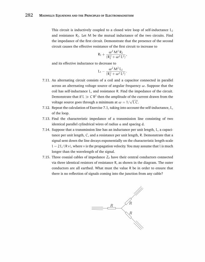
“chapter7” — 2007/12/14 — 12:08 — page 282 — #28
282 MAXWELL’S EQUATIONS AND THE PRINCIPLES OF ELECTROMAGNETISM
This circuit is inductively coupled to a closed wire loop of self-inductance L2and resistance R2. Let M be the mutual inductance of the two circuits. Find
the impedance of the first circuit. Demonstrate that the presence of the second
circuit causes the effective resistance of the first circuit to increase to
R1 +ω2M2 R2
(R 22 +ω2 L2),
and its effective inductance to decrease to
L1 −ω2M2 L2
(R 22 +ω2 L2).
7.11. An alternating circuit consists of a coil and a capacitor connected in parallel
across an alternating voltage source of angular frequency ω. Suppose that the
coil has self-inductance L, and resistance R. Find the impedance of the circuit.
Demonstrate that if L CR2 then the amplitude of the current drawn from the
voltage source goes through a minimum at ω = 1/√LC.
7.12. Repeat the calculation of Exercise 7.1, taking into account the self-inductance, L,
of the loop.
7.13. Find the characteristic impedance of a transmission line consisting of two
identical parallel cylindrical wires of radius a and spacing d.
7.14. Suppose that a transmission line has an inductance per unit length, L, a capaci-
tance per unit length, C, and a resistance per unit length, R. Demonstrate that a
signal sent down the line decays exponentially on the characteristic length-scale
l = 2 L/(R v), where v is the propagation velocity. You may assume that l is much
longer than the wavelength of the signal.
7.15. Three coaxial cables of impedance Z0 have their central conductors connected
via three identical resistors of resistance R, as shown in the diagram. The outer
conductors are all earthed. What must the value R be in order to ensure that
there is no reflection of signals coming into the junction from any cable?
RR
R
“chapter8” — 2007/12/14 — 12:12 — page 283 — #1
C h a p t e r 8ELECTROMAGNETICENERGY ANDMOMENTUM
8.1 INTRODUCTION
In this chapter, we shall demonstrate that Maxwell’s equations conserveboth energy and momentum.
8.2 ENERGY CONSERVATION
We have seen that the energy density of an electric field is given by [seeEquation (5.20)]
UE =ε0 E
2
2, (8.1)
whereas the energy density of a magnetic field satisfies [see Equa-tion (7.55)]
UB =B2
2µ0. (8.2)
This suggests that the energy density of a general electromagneticfield is
U =ε0 E
2
2+B2
2µ0. (8.3)
We are now in a position to demonstrate that the classical theory ofelectromagnetism conserves energy. We have already come across oneconservation law in electromagnetism: i.e.,
∂ρ
∂t+ ∇ · j = 0. (8.4)
This is the equation of charge conservation. Integrating over some vol-ume V, bounded by a surface S, and making use of Gauss’ theorem,
283

“chapter8” — 2007/12/14 — 12:12 — page 284 — #2
284 MAXWELL’S EQUATIONS AND THE PRINCIPLES OF ELECTROMAGNETISM
we obtain
−∂
∂t
∫V
ρdV =
∮S
j · dS. (8.5)
In other words, the rate of decrease of the charge contained in volumeV equals the net flux of charge across surface S. This suggests that anenergy conservation law for electromagnetism should have the form
−∂
∂t
∫V
UdV =
∮S
u · dS. (8.6)
Here, U is the energy density of the electromagnetic field, and u is theflux of electromagnetic energy (i.e., energy |u| per unit time, per unitcross-sectional area, passes a given point in the direction of u). Accord-ing to the above equation, the rate of decrease of the electromagneticenergy in volume V equals the net flux of electromagnetic energy acrosssurface S.
However, Equation (8.6) is incomplete, because electromagneticfields can gain or lose energy by interacting with matter. We need tofactor this into our analysis. We saw earlier (see Section 5.3) that therate of heat dissipation per unit volume in a conductor (the so-calledohmic heating rate) is E · j. This energy is extracted from electromag-netic fields, so the rate of energy loss of the fields in volume V due tointeraction with matter is
∫V
E · jdV. Thus, Equation (8.6) generalizes to
−∂
∂t
∫V
UdV =
∮S
u · dS +
∫V
E · jdV. (8.7)
From Gauss’ theorem, the above equation is equivalent to
∂U
∂t+ ∇ · u = −E · j. (8.8)
Let us now see if we can derive an expression of this form from Maxwell’sequations.
We start from the differential form of Ampere’s law (including thedisplacement current):
∇ × B = µ0 j + ε0µ0∂E∂t. (8.9)
Dotting this equation with the electric field yields
−E · j = −E · ∇ × Bµ0
+ ε0 E · ∂E∂t. (8.10)
“chapter8” — 2007/12/14 — 12:12 — page 285 — #3
CHAPTER 8 ELECTROMAGNETIC ENERGY AND MOMENTUM 285
This can be rewritten
−E · j = −E · ∇ × Bµ0
+∂
∂t
(ε0 E
2
2
). (8.11)
Now, from vector field theory,
∇ · (E × B) ≡ B · ∇ × E − E · ∇ × B, (8.12)
so
−E · j = ∇·(
E × Bµ0
)−
B · ∇ × Eµ0
+∂
∂t
(ε0 E
2
2
). (8.13)
The differential form of Faraday’s law yields
∇ × E = −∂B∂t, (8.14)
so
−E · j = ∇·(
E × Bµ0
)+ µ−1
0 B · ∂B∂t
+∂
∂t
(ε0 E
2
2
). (8.15)
This can be rewritten
−E · j = ∇·(
E × Bµ0
)+∂
∂t
(ε0 E
2
2+B2
2µ0
). (8.16)
Thus, we obtain the desired conservation law,
∂U
∂t+ ∇ · u = −E · j, (8.17)
where
U =ε0 E
2
2+B2
2µ0(8.18)
is the electromagnetic energy density, and
u =E × Bµ0
(8.19)
is the electromagnetic energy flux. The latter quantity is usually calledthe Poynting flux, after its discoverer.
Let us see whether our expression for the electromagnetic energy fluxmakes sense. We all know that if we stand in the sun we get hot. Thisoccurs because we absorb electromagnetic radiation emitted by the Sun.
“chapter8” — 2007/12/14 — 12:12 — page 286 — #4
286 MAXWELL’S EQUATIONS AND THE PRINCIPLES OF ELECTROMAGNETISM
So, radiation must transport energy. The electric and magnetic fieldsin electromagnetic radiation are mutually perpendicular, and are alsoperpendicular to the direction of propagation k (this is a unit vector).Furthermore, B = E/c. Equation (4.90) can easily be transformed intothe following relation between the electric and magnetic fields of anelectromagnetic wave:
E × B =E2
ck. (8.20)
Thus, the Poynting flux for electromagnetic radiation is
u =E2
µ0 ck = ε0 c E
2 k. (8.21)
This expression tells us that electromagnetic waves transport energyalong their direction of propagation, which seems to make sense.
The energy density of electromagnetic radiation is
U =ε0 E
2
2+B2
2µ0=ε0 E
2
2+
E2
2µ0 c2= ε0 E
2, (8.22)
using B = E/c. Note that the electric and magnetic fields in an electro-magnetic wave have equal energy densities. Since electromagnetic wavestravel at the speed of light, we would expect the energy flux through onesquare meter in one second to equal the energy contained in a volumeof length c and unit cross-sectional area: i.e., c times the energy density.Thus,
|u| = cU = ε0 c E2, (8.23)
which is in accordance with Equation (8.21).As another example, consider a straight cylindrical wire of radius a,
and uniform resistivity η. Suppose that the wire is coaxial with the z-axis.Let us adopt standard cylindrical polar coordinates (r, θ, z). If a currentof uniform density j = j ez flows down the wire then Ohm’s law tellsus that there is a uniform longitudinal electric field E = E ez within thewire, where E = η j. According to Ampere’s circuital law, the current alsogenerates a circulating magnetic field, inside the wire, of the form B =(µ0 r j/2) eθ. Hence, the Poynting flux, u = E × B/µ0, within the wirepoints radially inward, and is of magnitude u = η j2 r/2. The net energyflux into a cylindrical surface, coaxial with the wire, of radius r and lengthl is U = u2π r l = η j2 V(r), where V(r) = π r2 l is the volume enclosedby the surface. However, η j2 is the rate of electromagnetic energy loss
“chapter8” — 2007/12/14 — 12:12 — page 287 — #5
CHAPTER 8 ELECTROMAGNETIC ENERGY AND MOMENTUM 287
per unit volume, due to ohmic heating. Hence, η j2 V(r) represents thenet rate of electromagnetic energy loss due to ohmic heating in the regionlying within the cylindrical surface. Thus, we can see that this energyloss is balanced by the inward flux of electromagnetic energy across thesurface. This flux represents energy which is ultimately derived from thebattery which drives the current through the wire.
In the presence of diamagnetic and magnetic media, starting fromEquation (6.117), we can derive an energy conservation law of the form
∂U
∂t+ ∇ · u = −E · jt, (8.24)
via analogous steps to those used to derive Equation (8.17). Here, theelectromagnetic energy density is written
U =1
2E · D +
1
2B · H, (8.25)
which is consistent with Equation (8.18). The Poynting flux takes theform
u = E × H, (8.26)
which is consistent with Equation (8.19). Of course, the above expres-sions are only valid for linear dielectric and magnetic media.
8.3 ELECTROMAGNETIC MOMENTUM
We have seen that electromagnetic waves carry energy. It turns out thatthey also carry momentum. Consider the following argument, due toEinstein. Suppose that we have a railroad car of mass M and length Lwhich is free to move in one dimension—see Figure 8.1. Suppose thatelectromagnetic radiation of total energy E is emitted from one end ofthe car, propagates along the length of the car, and is then absorbed atthe other end. The effective mass of this radiation is m = E/c2 (fromEinstein’s famous relation E = mc2). At first sight, the process describedabove appears to cause the center of mass of the system to spontaneouslyshift. This violates the law of momentum conservation (assuming therailway car is subject to no horizontal external forces). The only way inwhich the center of mass of the system can remain stationary is if therailway car moves in the opposite direction to the direction of propagationof the radiation. In fact, if the car moves by a distance x then the centerof mass of the system is the same before and after the radiation pulse
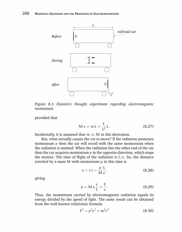
“chapter8” — 2007/12/14 — 12:12 — page 288 — #6
288 MAXWELL’S EQUATIONS AND THE PRINCIPLES OF ELECTROMAGNETISM
E
E
L
x
railroad carBefore
During
After
Figure 8.1: Einstein’s thought experiment regarding electromagneticmomentum.
provided that
Mx = mL =E
c2L. (8.27)
Incidentally, it is assumed that m M in this derivation.But, what actually causes the car to move? If the radiation possesses
momentum p then the car will recoil with the same momentum whenthe radiation is emitted. When the radiation hits the other end of the carthen the car acquires momentum p in the opposite direction, which stopsthe motion. The time of flight of the radiation is L/c. So, the distancetraveled by a mass M with momentum p in this time is
x = v t =p
M
L
c, (8.28)
giving
p = Mxc
L=E
c. (8.29)
Thus, the momentum carried by electromagnetic radiation equals itsenergy divided by the speed of light. The same result can be obtainedfrom the well-known relativistic formula
E2 = p2c2 +m2c4 (8.30)

“chapter8” — 2007/12/14 — 12:12 — page 289 — #7
CHAPTER 8 ELECTROMAGNETIC ENERGY AND MOMENTUM 289
relating the energy E, momentum p, and massm of a particle. Accordingto quantum theory, electromagnetic radiation is made up of masslessparticles called photons. Thus,
p =E
c(8.31)
for individual photons, so the same must be true of electromagneticradiation as a whole. It follows from Equation (8.29) that the momen-tum density g of electromagnetic radiation equals its energy densityover c, so
g =U
c=
|u|
c2=ε0 E
2
c. (8.32)
It is reasonable to suppose that the momentum points along the directionof the energy flow (this is obviously the case for photons), so the vectormomentum density (which gives the direction, as well as the magnitude,of the momentum per unit volume) of electromagnetic radiation is
g =uc2. (8.33)
Thus, the momentum density equals the energy flux over c2.Of course, the electric field associated with an electromagnetic wave
oscillates rapidly, which implies that the previous expressions for theenergy density, energy flux, and momentum density of electromagneticradiation are also rapidly oscillating. It is convenient to average overmany periods of the oscillation (this average is denoted 〈 〉). Thus,
〈U〉 =ε0 E
20
2, (8.34)
〈u〉 =c ε0 E
20
2k = c 〈U〉 k, (8.35)
〈g〉 =ε0 E
20
2 ck =
〈U〉c
k, (8.36)
where the factor 1/2 comes from averaging cos2(ωt). Here, E0 is thepeak amplitude of the electric field associated with the wave.
If electromagnetic radiation possesses momentum then it must exerta force on bodies which absorb (or emit) radiation. Suppose that a bodyis placed in a beam of perfectly collimated radiation, which it absorbscompletely. The amount of momentum absorbed per unit time, per unitcross-sectional area, is simply the amount of momentum contained in avolume of length c and unit cross-sectional area: i.e., c times the momen-tum density, g. An absorbed momentum per unit time, per unit area, is
“chapter8” — 2007/12/14 — 12:12 — page 290 — #8
290 MAXWELL’S EQUATIONS AND THE PRINCIPLES OF ELECTROMAGNETISM
equivalent to a pressure. In other words, the radiation exerts a pressurec g on the body. Thus, the radiation pressure is given by
p =ε0 E
2
2= 〈U〉. (8.37)
So, the pressure exerted by collimated electromagnetic radiation is equalto its average energy density.
Consider a cavity filled with electromagnetic radiation. What is theradiation pressure exerted on the walls? In this situation, the radiationpropagates in all directions with equal probability. Consider radiationpropagating at an angle θ to the local normal to the wall. The amountof such radiation hitting the wall per unit time, per unit area, is propor-tional to cos θ. Moreover, the component of momentum normal to thewall which the radiation carries is also proportional to cos θ. Thus, thepressure exerted on the wall is the same as in Equation (8.37), exceptthat it is weighted by the average of cos2 θ over all solid angles, in orderto take into account the fact that obliquely propagating radiation exertsa pressure which is cos2 θ times that of normal radiation. The average ofcos2 θ over all solid angles is 1/3, so for isotropic radiation
p =〈U〉3. (8.38)
Clearly, the pressure exerted by isotropic radiation is one third of itsaverage energy density.
The power incident on the surface of the Earth due to radiation emit-ted by the Sun is about 1300 W m−2. So, what is the radiation pressure?Since,
〈|u|〉 = c 〈U〉 = 1300W m−2, (8.39)
then
p = 〈U〉 4× 10⁻⁶ N m−2. (8.40)
Here, the radiation is assumed to be perfectly collimated. Thus, theradiation pressure exerted on the Earth is minuscule (for comparison,the pressure of the atmosphere is about 105 N m−2). Nevertheless, thissmall pressure due to radiation is important in outer space, since it isresponsible for continuously sweeping dust particles out of the SolarSystem. It is quite common for comets to exhibit two separate tails. One(called the gas tail) consists of ionized gas, and is swept along by the Solar
“chapter8” — 2007/12/14 — 12:12 — page 291 — #9
CHAPTER 8 ELECTROMAGNETIC ENERGY AND MOMENTUM 291
Wind (a stream of charged particles and magnetic field-lines emitted bythe Sun). The other (called the dust tail) consists of uncharged dustparticles, and is swept radially outward (since light travels in straight-lines) from the Sun by radiation pressure. Two separate tails are observedif the local direction of the Solar Wind is not radially outward from theSun (which is quite often the case).
The radiation pressure from sunlight is very weak. However, thatproduced by laser beams can be enormous (far higher than any con-ventional pressure which has ever been produced in a laboratory). Forinstance, the lasers used in Inertial Confinement Fusion (e.g., the NOVAexperiment in Lawrence Livermore National Laboratory) typically haveenergy fluxes of 1018 W m−2. This translates to a radiation pressure ofabout 104 atmospheres!
8.4 MOMENTUM CONSERVATION
It follows from Equations (8.19) and (8.33) that the momentum densityof electromagnetic fields can be written
g = ε0 E × B. (8.41)
Now, a momentum conservation equation for electromagnetic fieldsshould take the integral form
−∂
∂t
∫V
gi dV =
∫S
Gij dSj +
∫V
[ρE + j × B]i dV. (8.42)
Here, i and j run from 1 to 3 (1 corresponds to the x-direction, 2 tothe y-direction, and 3 to the z-direction). Moreover, the Einstein sum-mation convention is employed for repeated indices (e.g., aj aj ≡ a · a).Furthermore, the tensor Gij represents the flux of the ith componentof electromagnetic momentum in the j-direction. This tensor (a tensoris a direct generalization of a vector with two indices instead of one)is called the momentum flux density tensor. Hence, the above equationstates that the rate of loss of electromagnetic momentum in some vol-ume V is equal to the flux of electromagnetic momentum across thebounding surface S plus the rate at which momentum is transferred tomatter inside V. The latter rate is, of course, just the net electromagneticforce acting on matter inside V: i.e., the volume integral of the electro-magnetic force density, ρE + j × B. Now, a direct generalization of the
“chapter8” — 2007/12/14 — 12:12 — page 292 — #10
292 MAXWELL’S EQUATIONS AND THE PRINCIPLES OF ELECTROMAGNETISM
divergence theorem states that∫S
Gij dSj ≡∫V
∂Gij
∂xjdV, (8.43)
where x1 ≡ x, x2 ≡ y, etc. Hence, in differential form, our momentumconservation equation for electromagnetic fields is written
−∂
∂t[ε0 E × B]i =
∂Gij
∂xj+ [ρE + j × B]i. (8.44)
Let us now attempt to derive an equation of this form from Maxwell’sequations.
Maxwell’s equations are as follows:
∇ · E =ρ
ε0, (8.45)
∇ · B = 0, (8.46)
∇ × E = −∂B∂t, (8.47)
∇ × B = µ0 j + ε0µ0∂E∂t. (8.48)
We can cross Equation (8.48) divided by µ0 with B, and rearrange, togive
−ε0∂E∂t
× B =B × (∇ × B)
µ0+ j × B. (8.49)
Next, let us cross E with Equation (8.47) times ε0, rearrange, and addthe result to the above equation. We obtain
−ε0∂E∂t
× B − ε0 E × ∂B∂t
= ε0 E × (∇ × E) +B × (∇ × B)
µ0+ j × B.
(8.50)
Next, making use of Equations (8.45) and (8.46), we get
−∂
∂t[ε0 E × B] = ε0 E × (∇ × E) +
B × (∇ × B)
µ0
− ε0 (∇ · E) E −1
µ0(∇ · B) B + ρE + j × B. (8.51)
Now, from vector field theory,
∇(E2/2) ≡ E × (∇ × E) + (E · ∇)E, (8.52)
“chapter8” — 2007/12/14 — 12:12 — page 293 — #11
CHAPTER 8 ELECTROMAGNETIC ENERGY AND MOMENTUM 293
with a similar equation for B. Hence, Equation (8.51) takes the form
−∂
∂t[ε0 E × B] = ε0
[∇(E2/2) − (∇ · E) E − (E · ∇)E
]
+1
µ0
[∇(B2/2) − (∇ · B) B − (B · ∇)B
]+ ρE + j × B. (8.53)
Finally, when written in terms of components, the above equationbecomes
−∂
∂t[ε0 E × B]i =
∂
∂xj
[ε0 E
2 δij/2− ε0 Ei Ej + B2 δij/2 µ0 − Bi Bj/µ0
]+ [ρE + j × B]i , (8.54)
since [(∇ · E) E]i ≡ (∂Ej/∂xj)Ei, and [(E · ∇)E]i ≡ Ej (∂Ei/∂xj). Here, δijis a Kronecker delta symbol (i.e., δij = 1 if i = j, and δij = 0 otherwise).Comparing the above equation with Equation (8.44), we conclude thatthe momentum flux density tensor of electromagnetic fields takes theform
Gij = ε0 (E2 δij/2− Ei Ej) + (B2 δij/2− Bi Bj)/µ0. (8.55)
The momentum conservation equation (8.44) is sometimes written
[ρE + j × B]i =∂Tij
∂xj−∂
∂t[ε0 E × B]i , (8.56)
where
Tij = −Gij = ε0 (Ei Ej − E2 δij/2) + (Bi Bj − B
2 δij/2)/µ0 (8.57)
is called the Maxwell stress tensor.Consider a uniform electric field, E = E ez. According to Equa-
tion (8.55), the momentum flux density tensor of such a field is
G =
ε0 E
2/2 0 0
0 ε0 E2/2 0
0 0 −ε0 E2/2
. (8.58)
As is well-known, the momentum flux density tensor of a conventionalgas of pressure p is written
G =
p 0 0
0 p 0
0 0 p
. (8.59)
“chapter8” — 2007/12/14 — 12:12 — page 294 — #12
294 MAXWELL’S EQUATIONS AND THE PRINCIPLES OF ELECTROMAGNETISM
In other words, from any small volume element there is an equal out-ward momentum flux density p in all three Cartesian directions, whichsimply corresponds to an isotropic gas pressure, p. This suggests that apositive diagonal element in a momentum stress tensor corresponds toa pressure exerted in the direction of the corresponding Cartesian axis.Furthermore, a negative diagonal element corresponds to negative pres-sure, or tension, exerted in the direction of the corresponding Cartesianaxis. Thus, we conclude, from Equation (8.58), that electric field-linesact rather like mutually repulsive elastic bands: i.e., there is a pressureforce acting perpendicular to the field-lines which tries to push themapart, whilst a tension force acting along the field-lines simultaneouslytries to shorten them. As an example, we have seen that the normal elec-tric field E⊥ above the surface of a charged conductor exerts an outwardpressure ε0 E2⊥/2 on the surface. One way of interpreting this pressureis to say that it is due to the tension in the electric field-lines anchoredin the surface. Likewise, the force of attraction between the two platesof a charged parallel plate capacitor can be attributed to the tension inthe electric field-lines running between them.
It is easily demonstrated that the momentum flux density tensor ofa uniform magnetic field, B = B ez, is
G =
B2/2µ0 0 0
0 B2/2µ0 0
0 0 −B2/2µ0
. (8.60)
Hence, magnetic field-lines also act like mutually repulsive elastic bands.For instance, the uniform field B inside a conventional solenoid exerts anoutward pressure B2/2µ0 on the windings which generate and confine it.
8.5 ANGULAR MOMENTUM CONSERVATION
An electromagnetic field which possesses a momentum density g mustalso possess an angular momentum density
h = r × g. (8.61)
It follows that electromagnetic fields can exchange angular momentum,as well as linear momentum, with ordinary matter. As an illustration ofthis, consider the following famous example.

“chapter8” — 2007/12/14 — 12:12 — page 295 — #13
CHAPTER 8 ELECTROMAGNETIC ENERGY AND MOMENTUM 295
Suppose that we have two thin coaxial cylindrical conducting shellsof radii a and c, where a < c. Let the length of both cylinders be l. Sup-pose, further, that the cylinders are free to rotate independently abouttheir common axis. Finally, let the inner cylinder carry charge −Q, andthe outer cylinder charge +Q (where Q > 0). Now, suppose that a uni-form coaxial cylindrical solenoid winding of radius b (where a < b < c),and number of turns per unit length N, is placed between the two cylin-ders, and energized with a current I. Note that the total angular momen-tum of this system is a conserved quantity, since the system is isolated.
Consider an initial state in which both cylinders are stationary. Ramp-ing the solenoid current down to zero is observed to cause the two cylin-ders to start to rotate—the inner cylinder in the opposite sense to thesense of current circulation, and the outer cylinder in the same sense.In other words, the two cylinders acquire angular momentum when thecurrent in the solenoid coil is ramped down. Where does this angularmomentum come from? Clearly, it can only have come from the elec-tric and magnetic fields in the region between the cylinders. Let usinvestigate further.
It is convenient to define cylindrical polar coordinates (r, θ, z) whichare coaxial with the common axis of the two cylinders and the solenoidcoil. As is easily demonstrated from Gauss’ law, the electric field takesthe form E = Er er, where
Er =
−Q/(2πε0 r l) for a ≤ r ≤ c
0 otherwise. (8.62)
Likewise, it is easily shown from Ampere’s circuital law that the initialmagnetic field is written B = Bz ez, where
Bz =
µ0 N I for r ≤ b
0 otherwise. (8.63)
It follows from Equation (8.41) that the initial momentum density of theelectromagnetic field is g = gθ eθ, where
gθ =
µ0 N IQ/(2π r l) for a ≤ r ≤ b
0 otherwise. (8.64)
Hence, from Equation (8.61), the initial angular momentum density ofthe electromagnetic field is h = hz ez, where
hz =
µ0 N IQ/(2π l) for a ≤ r ≤ b
0 otherwise. (8.65)
“chapter8” — 2007/12/14 — 12:12 — page 296 — #14
296 MAXWELL’S EQUATIONS AND THE PRINCIPLES OF ELECTROMAGNETISM
In other words, the electromagnetic field possesses a uniform z-directedangular momentum density h in the region between the inner cylinderand the solenoid winding. It follows that the initial angular momentumcontent of the electromagnetic field, L, is equal to h multiplied by thevolume of this region. Hence, we obtain L = Lz ez, where
Lz =(b2 − a2)µ0 N IQ
2. (8.66)
Of course, as the current in the solenoid winding is ramped down thiselectromagnetic angular momentum is lost, and, presumably, transferredto the two cylinders. Let us examine how this transfer is effected.
Any change in the current flowing in the solenoid winding generatesan inductive electric field. From Faraday’s law, this field takes the formE = Eθ eθ, where
Eθ =
−µ0 N I r/2 for r ≤ b
−µ0 N Ib2/(2 r) otherwise
. (8.67)
This electric field exerts a torque Ta = Ta ez, where
Ta = −QEθ(a)a =µ0 N IQa
2
2, (8.68)
on the inner cylinder, and a torque Tb = Tb ez, where
Tb = QEθ(b)b = −µ0 N IQb
2
2, (8.69)
on the outer cylinder. Thus, the net angular momentum acquired by theinner cylinder, as the current in the solenoid coil is ramped down, isLa = La ez, where
La =
∫Ta dt = −
µ0 N IQa2
2. (8.70)
Likewise, the net angular momentum acquired by the outer cylinder isLb = Lb ez, where
Lb =
∫Tb dt =
µ0 N IQb2
2. (8.71)
Hence, the net angular momentum acquired by the two cylinders, as awhole, is L = Lz ez, where
Lz =(b2 − a2)µ0 N IQ
2. (8.72)
“chapter8” — 2007/12/14 — 12:12 — page 297 — #15
CHAPTER 8 ELECTROMAGNETIC ENERGY AND MOMENTUM 297
This, of course, is equal to the z-directed angular momentum lost by theelectromagnetic field.
8.6 EXERCISES
8.1. A solenoid consists of a wire wound uniformly around a solid cylindrical core of
radius a, length l, and permeability µ. Suppose that the wire has N turns per
unit length, and carries a current I. What is the energy stored within the core?
Suppose that the current in the wire is gradually ramped down. Calculate the
integral of the Poynting flux (due to the induced electric field) over the surface
of the core. Hence, demonstrate that the instantaneous rate of decrease of the
energy within the core is always equal to the integral of the Poynting flux over
its surface.
8.2. A coaxial cable consists of two thin coaxial cylindrical conducting shells of radii a
and b (where a < b). Suppose that the inner conductor carries the longitudinal
current I and the charge per unit length λ. Let the outer conductor carry equal
and opposite current and charge per unit length. What is the flux of electro-
magnetic energy and momentum down the cable (in the direction of the inner
current)? What is the electromagnetic pressure acting on the inner and outer
conductors?
8.3. Consider a coaxial cable consisting of two thin coaxial cylindrical conducting
shells of radii a and b (where a < b). Suppose that the inner conductor carries
current per unit length I, circulating in the plane perpendicular to its axis, and
charge per unit length λ. Let the outer conductor carry equal and opposite current
per unit length and charge per unit length. What is the flux of electromagnetic
angular momentum down the cable? What is the electromagnetic pressure acting
on the inner and outer conductors?
8.4. Calculate the electrostatic force acting between two identical point electrical
charges by finding the net electromagnetic momentum flux across a plane surface
located half-way between the charges. Verify that the result is consistent with
Coulomb’s law.
8.5. Calculate the magnetic force per unit length acting between two long paral-
lel straight wires carrying identical currents by finding the net electromagnetic
momentum flux across a plane surface located half-way between the wires. Verify
that the result is consistent with Ampere’s law.
8.6. Calculate the mean force acting on a perfect mirror of area A which reflects
normally incident electromagnetic radiation of peak electric field E0. Suppose
“chapter8” — 2007/12/14 — 12:12 — page 298 — #16
298 MAXWELL’S EQUATIONS AND THE PRINCIPLES OF ELECTROMAGNETISM
that the mirror only reflects a fraction f of the incident electromagnetic energy,
and absorbs the remainder. What now is the force acting on the mirror?
8.7. A thin spherical conducting shell of radius a carries a chargeQ. Use the concept
of electric field-line tension to find the force of repulsion between any two halves
of the shell.
8.8. A solid sphere of radius a carries a net charge Q which is uniformly distributed
over its volume. What is the force of repulsion between any two halves of the
sphere?
8.9. A U-shaped electromagnet of permeability µ 1, length l, pole separation d,
and uniform cross-sectional area A is energized by a current I flowing in a
winding withN turns. Find the force with which the magnet attracts a bar of the
same material which is placed over both poles (and completely covers them).
8.10. An iron sphere of radius a and uniform magnetization M = M ez carries an
electric charge Q. Find the net angular momentum of the electromagnetic field
surrounding the sphere. Suppose that the magnetization of the sphere decays to
zero. Demonstrate that the induced electric field exerts a torque on the sphere
which is such as to impart to it a mechanical angular momentum equal to that
lost by the electromagnetic field.
“chapter9” — 2007/11/30 — 11:11 — page 299 — #1
C h a p t e r 9 ELECTROMAGNETICRADIATION
9.1 INTRODUCTION
In this chapter, we shall employ Maxwell’s equations to investigate theemission, scattering, propagation, absorption, reflection, and refractionof electromagnetic radiation.
9.2 THE HERTZIAN DIPOLE
Consider two small spherical conductors connected by a wire. Sup-pose that electric charge flows periodically back and forth between thespheres. Let q(t) be the instantaneous charge on one of the conductors.The system is assumed to have zero net charge, so that the charge onthe other conductor is −q(t). Finally, let
q(t) = q0 sin (ωt). (9.1)
Now, we expect the oscillating current flowing in the wire connectingthe two spheres to generate electromagnetic radiation (see Section 4.11).Let us consider the simple case in which the length of the wire is smallcompared to the wavelength of the emitted radiation. If this is the casethen the current I flowing between the conductors has the same phasealong the whole length of the wire. It follows that
I(t) =dq
dt= I0 cos(ωt), (9.2)
where I0 = ωq0. This type of antenna is called a Hertzian dipole, afterthe German physicist Heinrich Hertz.
The magnetic vector potential generated by a current distributionj(r) is given by the well-known formula (see Section 4.12)
A(r, t) =µ0
4π
∫[j]
|r − r ′|d3r ′, (9.3)
299
“chapter9” — 2007/11/30 — 11:11 — page 300 — #2
300 MAXWELL’S EQUATIONS AND THE PRINCIPLES OF ELECTROMAGNETISM
where
[f] ≡ f(r ′, t− |r − r ′|/c). (9.4)
Suppose that the wire is aligned along the z-axis, and extendsfrom z = −l/2 to z = l/2. For a wire of negligible thickness, wecan replace j(r ′, t− |r − r ′|/c)d3r ′ by I(r ′, t− |r − r ′|/c)dz ′ ez. Thus,A(r, t) = Az(r, t) ez, and
Az(r, t) =µ0
4π
∫ l/2−l/2
I(z ′, t− |r − z ′ ez|/c)|r − z ′ ez|
dz ′. (9.5)
In the region r l,
|r − z ′ ez| r, (9.6)
and
t− |r − z ′ ez|/c t− r/c. (9.7)
The maximum error involved in the latter approximation is∆t ∼ l/c. Thiserror (which is a time) must be much less than a period of oscillationof the emitted radiation, otherwise the phase of the radiation will bewrong. So we require that
l
c 2π
ω, (9.8)
which implies that l λ, where λ = 2π c/ω is the wavelength of theemitted radiation. However, we have already assumed that the length ofthe wire l is much less than the wavelength of the radiation, and so theabove inequality is automatically satisfied. Thus, in the far field region,r λ, we can write
Az(r, t) µ0
4π
∫ l/2−l/2
I(z ′, t− r/c)
rdz ′. (9.9)
This integral is easy to perform, since the current is uniform along thelength of the wire. So, we get
Az(r, t) µ0 l
4π
I(t− r/c)
r. (9.10)
The scalar potential is most conveniently evaluated using the Lorenzgauge condition (see Section 4.12)
∇ · A = −ε0µ0∂φ
∂t. (9.11)

“chapter9” — 2007/11/30 — 11:11 — page 301 — #3
CHAPTER 9 ELECTROMAGNETIC RADIATION 301
Now,
∇ · A =∂Az
∂z µ0 l
4π
∂I(t− r/c)
∂t
(−z
r2 c
)+O
(1
r2
)(9.12)
to leading order in r−1. Thus, we obtain
φ(r, t) l
4πε0 c
z
r
I(t− r/c)
r. (9.13)
Given the vector and scalar potentials, Equations (9.10) and (9.13),respectively, we can evaluate the associated electric and magnetic fieldsusing (see Section 4.12)
E = −∂A∂t
− ∇φ, (9.14)
B = ∇ × A. (9.15)
Note that we are only interested in radiation fields, which fall off like r−1
with increasing distance from the source. It is easily demonstrated that
E −ωl I0
4πε0 c2sin θ
sin[ω (t− r/c)]
reθ, (9.16)
and
B −ωl I0
4πε0 c3sin θ
sin[ω (t− r/c)]
reϕ. (9.17)
Here, (r, θ,ϕ) are standard spherical polar coordinates aligned along thez-axis. The above expressions for the far-field (i.e., r λ) electromag-netic fields generated by a localized oscillating current are also easilyderived from Equations (4.190) and (4.191). Note that the fields aresymmetric in the azimuthal angle ϕ. Moreover, there is no radiationalong the axis of the oscillating dipole (i.e., θ = 0), and the maximumemission is in the plane perpendicular to this axis (i.e., θ = π/2)—seeFigure 9.1.
The average power crossing a spherical surface S (whose radius ismuch greater than λ), centered on the dipole, is
Prad =
∮S
〈u〉 · dS, (9.18)
where the average is over a single period of oscillation of the wave, andthe Poynting flux is given by (see Section 8.2)
u =E × Bµ0
=ω2 l2 I 2016π2ε0 c3
sin2[ω (t− r/c)]sin2 θr2
er. (9.19)
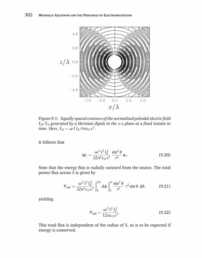
“chapter9” — 2007/11/30 — 11:11 — page 302 — #4
302 MAXWELL’S EQUATIONS AND THE PRINCIPLES OF ELECTROMAGNETISM
x/λ
z/λ
Figure 9.1: Equally spaced contours of the normalized poloidal electric fieldEθ/E0 generated by a Hertzian dipole in the x-z plane at a fixed instant intime. Here, E0 = ωl I0/4πε0 c
2.
It follows that
〈u〉 =ω2 l2 I 2032π2ε0 c3
sin2 θr2
er. (9.20)
Note that the energy flux is radially outward from the source. The totalpower flux across S is given by
Prad =ω2 l2 I 2032π2ε0 c3
∫ 2π0
dφ
∫π0
sin2 θr2
r2 sin θ dθ, (9.21)
yielding
Prad =ω2 l2 I 2012πε0 c3
. (9.22)
This total flux is independent of the radius of S, as is to be expected ifenergy is conserved.
“chapter9” — 2007/11/30 — 11:11 — page 303 — #5
CHAPTER 9 ELECTROMAGNETIC RADIATION 303
Recall that for a resistor of resistance R the average ohmic heatingpower is
Pheat = 〈I2 R〉 =1
2I 20 R, (9.23)
assuming that I = I0 cos(ωt). It is convenient to define the radiationresistance of a Hertzian dipole antenna:
Rrad =Prad
I 20 /2, (9.24)
so that
Rrad =2π
3ε0 c
(l
λ
)2, (9.25)
where λ = 2π c/ω is the wavelength of the radiation. In fact,
Rrad = 789
(l
λ
)2ohms. (9.26)
Now, in the theory of electrical circuits, an antenna is conventionallyrepresented as a resistor whose resistance is equal to the characteristicradiation resistance of the antenna plus its real resistance. The power lossI 20 Rrad/2 associated with the radiation resistance is due to the emissionof electromagnetic radiation, whereas the power loss I 20 R/2 associatedwith the real resistance is due to ohmic heating of the antenna.
Note that the formula (9.26) is only valid for l λ. This suggeststhat Rrad R for most Hertzian dipole antennas: i.e., the radiated poweris swamped by the ohmic losses. Thus, antennas whose lengths are muchless than that of the emitted radiation tend to be extremely inefficient. Infact, it is necessary to have l ∼ λ in order to obtain an efficient antenna.The simplest practical antenna is the half-wave antenna, for which l =λ/2. This can be analyzed as a series of Hertzian dipole antennas stackedon top of one another, each slightly out of phase with its neighbors. Thecharacteristic radiation resistance of a half-wave antenna is
Rrad =2.44
4πε0 c= 73 ohms. (9.27)
Antennas can also be used to receive electromagnetic radiation. Theincoming wave induces a voltage in the antenna, which can be detectedin an electrical circuit connected to the antenna. In fact, this processis equivalent to the emission of electromagnetic waves by the antenna
“chapter9” — 2007/11/30 — 11:11 — page 304 — #6
304 MAXWELL’S EQUATIONS AND THE PRINCIPLES OF ELECTROMAGNETISM
viewed in reverse. It is easily demonstrated that antennas most readilydetect electromagnetic radiation incident from those directions in whichthey preferentially emit radiation. Thus, a Hertzian dipole antenna isunable to detect radiation incident along its axis, and most efficientlydetects radiation incident in the plane perpendicular to this axis. In thetheory of electrical circuits, a receiving antenna is represented as a volt-age source in series with a resistor. The voltage source, V0 cos(ωt),represents the voltage induced in the antenna by the incoming wave.The resistor, Rrad, represents the power re-radiated by the antenna(here, the real resistance of the antenna is neglected). Let us repre-sent the detector circuit as a single load resistor, Rload, connected inseries with the antenna. So, what value of Rload ensures that the maxi-mum power is extracted from the wave and transmitted to the detectorcircuit?
According to Ohm’s law,
V = V0 cos(ωt) = I0 cos(ωt) (Rrad + Rload), (9.28)
where I = I0 cos(ωt) is the current induced in the circuit. The powerinput to the circuit is
Pin = 〈V I〉 =V 20
2 (Rrad + Rload). (9.29)
The power transferred to the load is
Pload = 〈I2 Rload〉 =Rload V
20
2 (Rrad + Rload)2. (9.30)
Finally, the power re-radiated by the antenna is
Prad = 〈I2 Rrad〉 =Rrad V
20
2 (Rrad + Rload)2. (9.31)
Note that Pin = Pload + Prad. The maximum power transfer to the loadoccurs when
∂Pload
∂Rload=V 202
[Rrad − Rload
(Rrad + Rload)3
]= 0. (9.32)
Thus, the maximum transfer rate corresponds to
Rload = Rrad. (9.33)
“chapter9” — 2007/11/30 — 11:11 — page 305 — #7
CHAPTER 9 ELECTROMAGNETIC RADIATION 305
In other words, the resistance of the load circuit must match the radiationresistance of the antenna. For this optimum case,
Pload = Prad =V 208 Rrad
=Pin
2. (9.34)
So, in the optimum case half of the power absorbed by the antenna isimmediately re-radiated. Clearly, an antenna which is receiving electro-magnetic radiation is also emitting it. This (allegedly) is how the BBCcatch people who do not pay their television license fee in the UnitedKingdom. They have vans which can detect the radiation emitted by aTV aerial whilst it is in use (they can even tell which channel you arewatching!).
For a Hertzian dipole antenna interacting with an incoming wavewhose electric field has an amplitude E0, we expect
V0 = E0 l. (9.35)
Here, we have used the fact that the wavelength of the radiation is muchlonger than the length of the antenna. We have also assumed that theantenna is properly aligned (i.e., the radiation is incident perpendicularto the axis of the antenna). The Poynting flux of the incoming wave is[see Equation (8.35)]
〈uin〉 =ε0 c E
20
2, (9.36)
whereas the power transferred to a properly matched detector circuit is
Pload =E20 l
2
8 Rrad. (9.37)
Consider an idealized antenna in which all incoming radiation incidenton some area Aeff is absorbed, and then magically transferred to thedetector circuit, with no re-radiation. Suppose that the power absorbedfrom the idealized antenna matches that absorbed from the real antenna.This implies that
Pload = 〈uin〉Aeff . (9.38)
The quantity Aeff is called the effective area of the antenna: it is the areaof the idealized antenna which absorbs as much net power from theincoming wave as the actual antenna. Thus,
Pload =E20 l
2
8 Rrad=ε0 c E
20
2Aeff , (9.39)

“chapter9” — 2007/11/30 — 11:11 — page 306 — #8
306 MAXWELL’S EQUATIONS AND THE PRINCIPLES OF ELECTROMAGNETISM
giving
Aeff =l2
4ε0 c Rrad=3
8πλ2. (9.40)
So, it is clear that the effective area of a Hertzian dipole antenna is oforder the wavelength squared of the incoming radiation.
For a properly aligned half-wave antenna,
Aeff = 0.13 λ2. (9.41)
Thus, the antenna, which is essentially one-dimensional with length λ/2,acts as if it is two-dimensional, with width 0.26 λ, as far as its absorptionof incoming electromagnetic radiation is concerned.
9.3 ELECTRIC DIPOLE RADIATION
In the previous section, we examined the radiation emitted by a shortelectric dipole of oscillating dipole moment
p(t) = p0 sin(ωt) ez, (9.42)
where p0 = q0 l = I0 l/ω. We found that, in the far field region, the meanelectromagnetic energy flux takes the form [see Equation (9.20)]
〈u〉 =ω4 p2032π2ε0 c3
sin2 θr2
er, (9.43)
assuming that the dipole is centered on the origin of our spherical polarcoordinate system. The mean power radiated into the element of solidangle dΩ = sin θdθdϕ, centered on the angular coordinates (θ, ϕ), is
dP = 〈u(r, θ,ϕ)〉·er r2 dΩ. (9.44)
Hence, the differential power radiated into this element of solid angle issimply
dP
dΩ=
ω4 p2032π2ε0 c3
sin2 θ. (9.45)
This formula completely specifies the radiation pattern of an oscillatingelectric dipole (provided that the dipole is much shorter in length thanthe wavelength of the emitted radiation). Of course, the power radiatedinto a given element of solid angle is independent of r, otherwise energywould not be conserved. Finally, the total radiated power is the integralof dP/dΩ over all solid angles.
“chapter9” — 2007/11/30 — 11:11 — page 307 — #9
CHAPTER 9 ELECTROMAGNETIC RADIATION 307
9.4 THOMPSON SCATTERING
Consider a plane electromagnetic wave of angular frequency ω inter-acting with a free electron of mass me and charge −e. Suppose that thewave is polarized such that its associated electric field is parallel to thez-axis: i.e.,
E = E0 sin(ωt) ez. (9.46)
Recall, from Section 4.7, that as long as the electron remains non-relativistic, the force exerted on it by the electromagnetic wave comespredominantly from the associated electric field. Hence, the electron’sequation of motion can be written
med2z
dt2= −e E0 sin(ωt), (9.47)
which can be solved to give
z =e E0
me ω2sin(ωt). (9.48)
So, in response to the wave, the electron oscillates backward and forwardin the direction of the wave electric field. It follows that the electroncan be thought of as a sort of oscillating electric dipole, with dipolemoment
p = −e z ez = −p0 sin(ωt) ez, (9.49)
where p0 = e2 E0/(meω2). (For the moment, let us not worry about
the positively charged component of the dipole.) Now, we know thatan oscillating electric dipole emits electromagnetic radiation. Hence, itfollows that a free electron placed in the path of a plane electromagneticwave will radiate. To be more exact, the electron scatters electromagneticradiation from the wave, since the radiation emitted by the electron is notnecessarily in the same direction as the wave, and any energy radiated bythe electron is ultimately extracted from the wave. This type of scatteringis called Thompson scattering.
It follows from Equation (9.45) that the differential power scatteredfrom a plane electromagnetic wave by a free electron into solid angledΩ takes the form
dP
dΩ=
e4 E2032π2ε0 c3 m2
e
sin2 θ. (9.50)
“chapter9” — 2007/11/30 — 11:11 — page 308 — #10
308 MAXWELL’S EQUATIONS AND THE PRINCIPLES OF ELECTROMAGNETISM
Now, the mean energy flux of the incident electromagnetic wave iswritten
|〈u〉| = c ε0 E20
2. (9.51)
It is helpful to introduce a quantity called the differential scattering cross-section. This is defined
dσ
dΩ=dP/dΩ
|〈u〉| , (9.52)
and has units of area over solid angle. Somewhat figuratively, we canthink of the electron as offering a target of area dσ/dΩ to the incidentwave. Any wave energy which falls on this target is scattered into thesolid angle dΩ. Likewise, we can also define the total scattering cross-section,
σ =
∮dσ
dΩdΩ, (9.53)
which has units of area. Again, the electron effectively offers a target ofarea σ to the incident wave. Any wave energy which falls on this targetis scattered in some direction or other. It follows from Equations (9.50)and (9.51) that the differential scattering cross-section for Thompsonscattering is
dσ
dΩ= r 2e sin2 θ, (9.54)
where the characteristic length
re =e2
4πε0 me c2= 2.82× 10⁻¹⁵ m (9.55)
is called the classical electron radius. An electron effectively acts like it hasa spatial extent re as far as its iteration with electromagnetic radiationis concerned. As is easily demonstrated, the total Thompson scatteringcross-section is
σT =8 π
3r 2e = 6.65× 10⁻²⁹ m2. (9.56)
Note that both the differential and the total Thompson scattering cross-sections are completely independent of the frequency (or wavelength) ofthe incident radiation.
A scattering cross-section of 10−28 m2 does not sound like much.Nevertheless, Thompson scattering is one of the most important types
“chapter9” — 2007/11/30 — 11:11 — page 309 — #11
CHAPTER 9 ELECTROMAGNETIC RADIATION 309
of scattering in the Universe. Consider the Sun. It turns out that themean mass density of the Sun is similar to that of water: i.e., about103 kg m−3. Hence, assuming that the Sun is predominantly made upof ionized Hydrogen, the mean number density of electrons in the Sun(which, of course, is the same as the number density of protons) isapproximately ne ∼ 103/mp ∼ 1030 m−3, wheremp ∼ 10−27 kg is the massof a proton. Let us consider how far, on average, a photon in the Suntravels before being scattered by a free electron. If we think of an indi-vidual photon as sweeping out a cylinder of cross-sectional area σT , thenthe photon will travel an average length l, such that a cylinder of areaσT and length l contains about one free electron, before being scattered.Hence, σT l ne ∼ 1, or
l ∼1
ne σT∼ 1 cm. (9.57)
Given that the radius of the Sun is approximately 109 m, it is clear thatsolar photons are very strongly scattered by free electrons. In fact, itcan easily be demonstrated that it takes a photon emitted in the solarcore many thousands of years to fight its way to the surface because ofThompson scattering.
After the “Big Bang,” when the Universe was very hot, it con-sisted predominately of ionized Hydrogen (and dark matter), and wasconsequently opaque to electromagnetic radiation, due to Thompsonscattering. However, as the Universe expanded, it also cooled, and even-tually became sufficiently cold (when the mean temperature was about1000C) for any free protons and electrons to combine to form molec-ular Hydrogen. It turns out that molecular Hydrogen does not scatterradiation anything like as effectively as free electrons (see the nextsection). Hence, as soon as the Universe became filled with molecu-lar Hydrogen, it effectively became transparent to radiation. Indeed, theso-called cosmic microwave background is the remnant of radiation whichwas last scattered when the Universe was filled with ionized Hydrogen(i.e., when it was about 1000C). Astronomers can gain a great deal ofinformation about the conditions in the early Universe by studying thisradiation.
Incidentally, it is clear from Equations (9.55) and (9.56) that thescattering cross-section of a free particle of charge q and mass m isproportional to q4/m2. It follows that the scattering of electromagneticradiation by free electrons is generally very much stronger than thescattering by free protons (assuming that the number densities of bothspecies are similar).
“chapter9” — 2007/11/30 — 11:11 — page 310 — #12
310 MAXWELL’S EQUATIONS AND THE PRINCIPLES OF ELECTROMAGNETISM
9.5 RAYLEIGH SCATTERING
Let us now consider the scattering of electromagnetic radiation by neu-tral atoms. For instance, consider a Hydrogen atom. The atom consistsof a light electron and a massive proton. As we have seen, the elec-tron scatters radiation much more strongly than the proton, so let usconcentrate on the response of the electron to an incident electromag-netic wave. Suppose that the wave electric field is again polarized in thez-direction, and is given by Equation (9.46). We can approximate theelectron’s equation of motion as
med2z
dt2= −meω
20 z− e E0 sin(ωt). (9.58)
Here, the second term on the right-hand side represents the perturbingforce due to the electromagnetic wave, whereas the first term representsthe (linearized) force of electrostatic attraction between the electronand the proton. Here, we are very crudely modeling our Hydrogen atomas a simple harmonic oscillator of natural frequency ω0. We can thinkof ω0 as the typical frequency of electromagnetic radiation emitted bythe atom after it is transiently disturbed. In other words, in our model,ω0 should match the frequency of one of the spectral lines of Hydro-gen. More generally, we can extend the above model to deal with justabout any type of atom, provided that we set ω0 to the frequency of aspectral line.
We can easily solve Equation (9.58) to give
z =e E0
me (ω2 −ω20 )
sin(ωt). (9.59)
Hence, the dipole moment of the electron takes the form p =−p0 sin(ωt) ez, where
p0 =e2 E0
me (ω2 −ω20 ). (9.60)
It follows, by analogy with the analysis in the previous section, that thedifferential and total scattering cross-sections of our model atom takethe form
dσ
dΩ=
ω4
(ω2 −ω20 )2r 2e sin2 θ, (9.61)
“chapter9” — 2007/11/30 — 11:11 — page 311 — #13
CHAPTER 9 ELECTROMAGNETIC RADIATION 311
and
σ =ω4
(ω2 −ω20 )2σT , (9.62)
respectively.In the limit in which the frequency of the incident radiation is much
greater than the natural frequency of the atom, Equations (9.61) and(9.62) reduce to the previously obtained expressions for scattering by afree electron. In other words, an electron in an atom acts very much like afree electron as far as high-frequency radiation is concerned. In the oppo-site limit, in which the frequency of the incident radiation is much lessthan the natural frequency of the atom, Equations (9.61) and (9.62) yield
dσ
dΩ=
(ω
ω0
)4r 2e sin2 θ, (9.63)
and
σ =
(ω
ω0
)4σT , (9.64)
respectively. This type of scattering is called Rayleigh scattering. There aretwo features of Rayleigh scattering which are worth noting. First of all,it is much weaker than Thompson scattering (since ω ω0). Secondly,unlike Thompson scattering, it is highly frequency dependent. Indeed,it is clear, from the above formulae, that high-frequency (short wave-length) radiation is scattered far more effectively than low-frequency(long wavelength) radiation.
The most common example of Rayleigh scattering is the scatteringof visible radiation from the Sun by neutral atoms (mostly Nitrogen andOxygen) in the upper atmosphere. The frequency of visible radiation ismuch less than the typical emission frequencies of a Nitrogen or Oxygenatom (which lie in the ultraviolet band), so it is certainly the case thatω ω0. When the Sun is low in the sky, radiation from it has to traversea comparatively long path through the atmosphere before reaching us.Under these circumstances, the scattering of direct solar light by neutralatoms in the atmosphere becomes noticeable (it is not noticeable whenthe Sun is high is the sky, and radiation from it consequently only has totraverse a relatively short path through the atmosphere before reachingus). According to Equation (9.64), blue light is scattered slightly morestrongly than red light (since blue light has a slightly higher frequency

“chapter9” — 2007/11/30 — 11:11 — page 312 — #14
312 MAXWELL’S EQUATIONS AND THE PRINCIPLES OF ELECTROMAGNETISM
than red light). Hence, when the Sun is low in the sky, it appears lessbright, due to atmospheric scattering. However, it also appears redderthan normal, because more blue light than red light is scattered out ofthe solar light-rays, leaving an excess of red light. Likewise, when welook up at the daytime sky, it does not appear black (like the sky on theMoon) because of light from solar radiation which grazes the atmospherebeing scattered downward toward the surface of the Earth. Again, sinceblue light is scattered more effectively than red light, there is an excessof blue light scattered downward, and so the daytime sky appears blue.
Light from the Sun is unpolarized. However, when it is scatteredit becomes polarized, because light is scattered preferentially in somedirections rather than others. Consider a light-ray from the Sun whichgrazes the Earth’s atmosphere. The light-ray contains light which is polar-ized such that the electric field is vertical to the ground, and light whichis polarized such that the electric field is horizontal to the ground (andperpendicular to the path of the light-ray), in equal amounts. However,due to the sin2 θ factor in the dipole emission formula (9.45) (where, inthis case, θ is the angle between the direction of the wave electric fieldand the direction of scattering), very little light is scattered downwardfrom the vertically polarized light compared to the horizontally polarizedlight. Moreover, the light scattered from the horizontally polarization issuch that its electric field is preferentially perpendicular, rather thanparallel, to the direction of propagation of the solar light-ray (i.e., thedirection to the Sun). Consequently, the blue light from the daytime skyis preferentially polarized in a direction perpendicular to the direction tothe Sun.
9.6 PROPAGATION IN A DIELECTRIC MEDIUM
Consider the propagation of an electromagnetic wave through a uniformdielectric medium of dielectric constant ε. According to Equations (6.12)and (6.14), the dipole moment per unit volume induced in the mediumby the wave electric field E is
P = ε0 (ε− 1) E. (9.65)
There are no free charges or free currents in the medium. There is alsono bound charge density (since the medium is uniform), and no magne-tization current density (since the medium is non-magnetic). However,there is a polarization current due to the time-variation of the induced
“chapter9” — 2007/11/30 — 11:11 — page 313 — #15
CHAPTER 9 ELECTROMAGNETIC RADIATION 313
dipole moment per unit volume. According to Equation (6.109), thiscurrent is given by
jp =∂P∂t. (9.66)
Hence, Maxwell’s equations take the form
∇·E = 0, (9.67)
∇·B = 0, (9.68)
∇ × E = −∂B∂t, (9.69)
∇ × B = µ0 jp + ε0 µ0∂E∂t. (9.70)
According to Equations (9.65) and (9.66), the last of the above equationscan be rewritten
∇ × B = ε0 µ0 (ε− 1)∂E∂t
+ ε0 µ0∂E∂t
=ε
c2∂E∂t, (9.71)
since c = (ε0 µ0)−1/2. Thus, Maxwell’s equations for the propagation of
electromagnetic waves through a dielectric medium are the same asMaxwell’s equations for the propagation of waves through a vacuum(see Section 4.7), except that c → c/n, where
n =√ε (9.72)
is called the refractive index of the medium in question. Hence, we con-clude that electromagnetic waves propagate through a dielectric mediumslower than through a vacuum by a factor n (assuming, of course,that n > 1). This conclusion (which was reached long before Maxwell’sequations were invented) is the basis of all geometric optics involvingrefraction.
9.7 DIELECTRIC CONSTANT OF A GASEOUS MEDIUM
In Section 9.5, we discussed a rather crude model of an atom interact-ing with an electromagnetic wave. According to this model, the dipolemoment p of the atom induced by the wave electric field E is given by
p =e2
me (ω20 −ω2)
E, (9.73)
“chapter9” — 2007/11/30 — 11:11 — page 314 — #16
314 MAXWELL’S EQUATIONS AND THE PRINCIPLES OF ELECTROMAGNETISM
where ω0 is the natural frequency of the atom (i.e., the frequency ofone of the atom’s spectral lines), and ω the frequency of the incidentradiation. Suppose that there are n atoms per unit volume. It followsthat the induced dipole moment per unit volume of the assemblage ofatoms takes the form
P =ne2
me (ω20 −ω2)
E. (9.74)
Finally, a comparison with Equation (9.65) yields the following expres-sion for the dielectric constant of the collection of atoms,
ε = 1+ne2
ε0 me (ω20 −ω2)
. (9.75)
The above formula works fairly well for dilute gases, although it is, ofcourse, necessary to sum over all species and all important spectral lines.
Note that, in general, the dielectric “constant” of a gaseous medium(as far as electromagnetic radiation is concerned) is a function of thewave frequency, ω. Since the effective wave propagation speed throughthe medium is c/
√ε, it follows that waves of different frequencies travel
through a gaesous medium at different speeds. This phenomenon iscalled dispersion, since it can be shown to cause short wave-pulses tospread out as they propagate through the medium. At low frequencies(ω ω0), however, our expression for ε becomes frequency indepen-dent, and so there is no dispersion of low-frequency waves by a gaseousmedium.
9.8 DISPERSION RELATION OF A PLASMA
A plasma is very similar to a gaseous medium, expect that the electronsare free: i.e., there is no restoring force due to nearby atomic nuclii.Hence, we can obtain an expression for the dielectric constant of a plasmafrom Equation (9.75) by settingω0 to zero, and n to the number densityof electrons, ne. We obtain
ε = 1−ω2p
ω2, (9.76)
where the characteristic frequency
ωp =
√ne e2
ε0 me(9.77)
“chapter9” — 2007/11/30 — 11:11 — page 315 — #17
CHAPTER 9 ELECTROMAGNETIC RADIATION 315
is called the plasma frequency. We can immediately see that formula(9.76) is problematic. For frequencies above the plasma frequency, thedielectric constant of a plasma is less than unity. Hence, the refractiveindex n =
√ε is also less than unity. This would seem to imply that high-
frequency electromagnetic waves can propagate through a plasma witha velocity c/n which is greater than the velocity of light in a vacuum.This appears to violate one of the principles of Relativity. On the otherhand, for frequencies below the plasma frequency, the dielectric constantis negative, which would seem to imply that the refractive index n =
√ε
is imaginary. How should we interpret this?Consider an infinite plane-wave of frequency ω, which is greater
than the plasma frequency, propagating through a plasma. Suppose thatthe wave electric field takes the form
E = E0 e i (k x−ωt) ez, (9.78)
where it is understood that the physical electric field is the real part ofthe above expression. A peak or trough of the above wave travels at theso-called phase-velocity, which is given by
vp =ω
k. (9.79)
Now, we have also seen that the phase-velocity of electromagnetic wavesin a dielectric medium is vp = c/n = c/
√ε, so
ω2 =k2 c2
ε. (9.80)
It follows from Equation (9.76) that
ω2 = k2 c2 +ω2p (9.81)
in a plasma. The above type of expression, which effectively determinesthe wave frequency, ω, as a function of the wave-number, k, for themedium in question, is called a dispersion relation (since, amongst otherthings, it determines how fast wave-pulses disperse in the medium).According to the above dispersion relation, the phase-velocity of high-frequency waves propagating through a plasma is given by
vp =c√
1−ω2p/ω
2, (9.82)
which is indeed greater than c. However, the Theory of Relativity doesnot forbid this. What the Theory of Relativity says is that information
“chapter9” — 2007/11/30 — 11:11 — page 316 — #18
316 MAXWELL’S EQUATIONS AND THE PRINCIPLES OF ELECTROMAGNETISM
cannot travel at a velocity greater than c. However, the peaks and troughsof an infinite plane-wave, such as (9.78), do not carry any information.
We now need to consider how we could transmit informationthrough a plasma (or any other dielectric medium) by means of elec-tromagnetic waves. The easiest way would be to send a series of shortdiscrete wave-pulses through the plasma, so that we could transmit infor-mation in a sort of Morse code. We can build up a wave-pulse from asuitable superposition of infinite plane-waves of different frequenciesand wavelengths: e.g.,
Ez(x, t) =
∫F(k) e iφ(k) dk, (9.83)
where φ(k) = k x−ω(k) t, and ω(k) is determined from the dispersionrelation (9.81). Now, it turns out that a relatively short wave-pulse canonly be built up from a superposition of plane-waves with a relativelywide range of different k values. Hence, for a short wave-pulse, theintegrand in the above formula consists of the product of a fairly slowlyvarying function, F(k), and a rapidly oscillating function, exp[iφ(k)]. Thelatter function is rapidly oscillating because the phase φ(k) varies veryrapidly with k, relative to F(k). We expect the net result of integrating theproduct of a slowly varying function and rapidly oscillating function to besmall, since the oscillations will generally average to zero. It follows thatthe integral (9.83) is dominated by those regions of k-space for whichφ(k) varies least rapidly with k. Hence, the peak of the wave-pulse mostlikely corresponds to a maximum or minimum of φ(k): i.e.,
dφ
dk= x−
dω
dkt = 0. (9.84)
Thus, we infer that the velocity of the wave-pulse (which corresponds tothe velocity of the peak) is given by
vg =dω
dk. (9.85)
This velocity is called the group-velocity, and is different to the phase-velocity in dispersive media: i.e., media for which ω is not directlyproportional to k. (Of course, in a vacuum, ω = k c, so the phaseand group velocities are both equal to c.) The upshot of the abovediscussion is that information (i.e., an individual wave-pulse) travelsthrough a dispersive media at the group-velocity, rather than the phase-velocity. Hence, Relativity demands that the group-velocity, rather thanthe phase-velocity, must always be less than c.
“chapter9” — 2007/11/30 — 11:11 — page 317 — #19
CHAPTER 9 ELECTROMAGNETIC RADIATION 317
What is the group-velocity for high-frequency waves propagatingthrough a plasma? Well, differentiation of the dispersion relation (9.81)yields
ω
k
dω
dk= vp vg = c2. (9.86)
Hence, it follows from Equation (9.82) that
vg = c
√1−
ω2p
ω2, (9.87)
which is less than c. We thus conclude that the dispersion relation (9.81)is indeed consistent with Relativity.
Let us now consider the propagation of low-frequency electromag-netic waves through a plasma. We can see, from Equations (9.82) and(9.87), that when the wave frequency, ω, falls below the plasma fre-quency, ωp, both the phase and group velocities become imaginary.This indicates that the wave attenuates as it propagates. Consider, forinstance, a plane-wave of frequencyω < ωp. According to the dispersionrelation (9.81), the associated wave-number is given by
k = i√ω2p −ω2
/c = i |k|. (9.88)
Hence, the wave electric field takes the form
Ez = E0 e i (i |k| x−ωt) = E0 e−|k| x e−iωt. (9.89)
So, it can be seen that for ω < ωp electromagnetic waves in a plasmatake the form of decaying standing waves, rather than traveling waves.We conclude that an electromagnetic wave, of frequency less than theplasma frequency, which is incident on a plasma will not propagatethrough the plasma. Instead, it will be totally reflected.
We can be sure that the incident wave is reflected by the plasma,rather than absorbed, by considering the energy flux of the wave in theplasma. It is easily demonstrated that the energy flux of an electromag-netic wave can be written
u =E × Bµ0
=E2
µ0 ωk. (9.90)
For a wave with a real frequency and a complex k-vector, the aboveformula generalizes to
u =|E|2
µ0 ωRe(k). (9.91)
“chapter9” — 2007/11/30 — 11:11 — page 318 — #20
318 MAXWELL’S EQUATIONS AND THE PRINCIPLES OF ELECTROMAGNETISM
However, according to Equation (9.88), the k-vector for a low-frequencyelectromagnetic wave in a plasma is purely imaginary. It follows that theassociated energy flux is zero. Hence, any low-frequency wave which isincident on the plasma must be totally reflected, since if there were anyabsorption of the wave energy then there would be a net energy flux intothe plasma.
The outermost layer of the Earth’s atmosphere consists of a partiallyionized zone known as the ionosphere. The plasma frequency in the iono-sphere is about 1 MHz, which lies at the upper end of the medium-waveband of radio frequencies. It follows that low-frequency radio signals(i.e., all signals in the long-wave band, and most in the medium-waveband) are reflected off the ionosphere. For this reason, such signals canbe detected over the horizon. Indeed, long-wave radio signals reflectmultiple times off the ionosphere with very little loss (they also reflectmultiple times off the Earth, which is enough of a conductor to act asa mirror for radio waves), and can consequently be detected all overthe world. On the other hand, high-frequency radio signals (i.e., allsignals in the FM band) pass straight through the ionosphere. For thisreason, such signals cannot be detected over the horizon, which accountsfor the relatively local coverage of FM radio stations. Note, from Equa-tion (9.77), that the plasma frequency is proportional to the square rootof the number density of free electrons. Now, the level of ionization inthe ionosphere is maintained by ultraviolet light from the Sun (whicheffectively knocks electrons out of neutral atoms). Of course, there isno such light at night, and the number density of free electrons in theionosphere consequently drops as electrons and ions gradually recom-bine. It follows that the plasma frequency in the ionosphere also dropsat night, giving rise to a marked deterioration in the reception of distantmedium-wave radio stations.
9.9 FARADAY ROTATION
Consider a high-frequency electromagnetic wave propagating, along thez-axis, through a plasma with a longitudinal equilibrium magnetic field,B = B0 ez. The equation of motion of an individual electron making upthe plasma takes the form
medvdt
= −e (E + B0 v × ez), (9.92)
“chapter9” — 2007/11/30 — 11:11 — page 319 — #21
CHAPTER 9 ELECTROMAGNETIC RADIATION 319
where the first term on the right-hand side is due to the wave electricfield, and the second to the equilibrium magnetic field. (As usual, wecan neglect the wave magnetic field, provided that the electron motionremains non-relativistic.) Of course, v = dr/dt, where r is the electrondisplacement from its equilibrium position. Suppose that all perturbedquantities vary with time like exp(−iωt), whereω is the wave frequency.It follows that
meω2 x = e (Ex − iωB0 y), (9.93)
meω2 y = e (Ey + iωB0 x). (9.94)
It is helpful to define
s± = x± iy, (9.95)
E± = Ex ± iEy. (9.96)
Using these new variables, Equations (9.93) and (9.94) can be rewritten
meω2 s± = e (E± ∓ωB0 s±), (9.97)
which can be solved to give
s± =e E±
meω (ω±Ω), (9.98)
where Ω = eB0/me is the so-called cyclotron frequency (i.e., the charac-teristic gyration frequency of free electrons in the equilibrium magneticfield—see Section 3.7).
In terms of s±, the electron displacement can be written
r = s+ e i (k+ z−ωt) e+ + s− e i (k− z−ωt) e−, (9.99)
where
e± =1
2(ex ∓ i ey) . (9.100)
Likewise, in terms of E±, the wave electric field takes the form
E = E+ e i (k+ z−ωt) e+ + E− e i (k− z−ωt) e−. (9.101)
Obviously, the actual displacement and electric field are the real parts ofthe above expressions. It follows from Equation (9.101) that E+ corre-sponds to a constant amplitude electric field which rotates clockwise inthe x-y plane (looking down the z-axis) as the wave propagates in the+z-direction, whereas E− corresponds to a constant amplitude electric
“chapter9” — 2007/11/30 — 11:11 — page 320 — #22
320 MAXWELL’S EQUATIONS AND THE PRINCIPLES OF ELECTROMAGNETISM
field which rotates counter clockwise. The former type of wave is termedleft-hand circularly polarized, whereas the latter is termed right-handcircularly polarized. Note also that s+ and s− correspond to circular elec-tron motion in opposite senses. With these insights, we conclude thatEquation (9.98) indicates that individual electrons in the plasma havea slightly different response to left- and right-hand circularly polarizedwaves in the presence of a longitudinal magnetic field.
Following the analysis of Section 9.7, we can deduce from Equa-tion (9.98) that the dielectric constant of the plasma for left- andright-hand circularly polarized waves is
ε± = 1−ω2p
ω (ω±Ω), (9.102)
respectively. Hence, according to Equation (9.80), the dispersion relationfor left- and right-hand circularly polarized waves becomes
k2± c2 = ω2
[1−
ω2p
ω (ω±Ω)
], (9.103)
respectively. In the limit ω ωp,Ω, we obtain
k± k± ∆k, (9.104)
where k = ω [1− (1/2)ω2p/ω
2]/c and ∆k = (1/2) (ω2p/ω
2)Ω/c. Inother words, in a magnetized plasma, left- and right-hand circu-larly polarized waves of the same frequency have slightly differentwave-numbers.
Let us now consider the propagation of a linearly polarized electro-magnetic wave through the plasma. Such a wave can be constructedvia a superposition of left- and right-hand circularly polarized waves ofequal amplitudes. So, the wave electric field can be written
E = E0
[e i (k+ z−ωt) e+ + e i (k− z−ωt) e−
]. (9.105)
It can easily be seen that at z = 0 the wave electric field is aligned alongthe x-axis. If left- and right-hand circularly polarized waves of the samefrequency have the same wave-number (i.e., if k+ = k−) then the waveelectric field will continue to be aligned along the x-axis as the wave prop-agates in the +z-direction: i.e., we will obtain a standard linearly polar-ized wave. However, we have just demonstrated that, in the presence ofa longitudinal magnetic field, the wave-numbers k+ and k− are slightlydifferent. What effect does this have on the polarization of the wave?
“chapter9” — 2007/11/30 — 11:11 — page 321 — #23
CHAPTER 9 ELECTROMAGNETIC RADIATION 321
Taking the real part of Equation (9.105), and making use of Equation(9.104), and some standard trigonometrical identities, we obtain
E = E0 [cos(k z−ωt) cos(∆k z), cos(k z−ωt) sin(∆k z), 0] . (9.106)
The polarization angle of the wave (which is a convenient measure ofits plane of polarization) is given by
ϕ = tan−1(Ey/Ex) = ∆k z. (9.107)
Thus, we conclude that in the presence of a longitudinal magneticfield the polarization angle rotates as the wave propagates through theplasma. This effect is known as Faraday rotation. It is clear, from theabove expression, that the rate of advance of the polarization angle withdistance travelled by the wave is given by
dϕ
dz= ∆k =
ω2p Ω
2ω2 c=
e3
2ε0 m2e c
ne B0
ω2. (9.108)
Hence, a linearly polarized electromagnetic wave which propagatesthrough a plasma with a (slowly) varying electron number density, ne(z),and longitudinal magnetic field, B0(z), has its plane of polarizationrotated through a total angle
∆ϕ = ϕ−ϕ0 =e3
2ε0 m2e c
1
ω2
∫ne(z)B0(z)dz. (9.109)
Note the very strong inverse variation of ∆ϕ with ω.Pulsars are rapidly rotating neutron stars which emit regular blips
of highly polarized radio waves. Hundreds of such objects have beenfound in our galaxy since the first was discovered in 1967. By measuringthe variation of the angle of polarization, ϕ, of radio emission from apulsar with frequency,ω, astronomers can effectively determine the lineintegral of ne B0 along the straight-line joining the pulsar to the Earthusing formula (9.109). Here, ne is the number density of free electronsin the interstellar medium, whereas B0 is the parallel component of thegalactic magnetic field. Obviously, in order to achieve this, astronomersmust make the reasonable assumption that the radiation was emitted bythe pulsar with a common angle of polarization, ϕ0, over a wide rangeof different frequencies. By fitting Equation (9.109) to the data, andthen extrapolating to large ω, it is then possible to determine ϕ0, and,hence, the amount, ∆ϕ(ω), through which the polarization angle of theradiation has rotated, at a given frequency, during its passage to Earth.
“chapter9” — 2007/11/30 — 11:11 — page 322 — #24
322 MAXWELL’S EQUATIONS AND THE PRINCIPLES OF ELECTROMAGNETISM
9.10 PROPAGATION IN A CONDUCTOR
Consider the propagation of an electromagnetic wave through a con-ducting medium which obeys Ohm’s law:
j = σE. (9.110)
Here, σ is the conductivity of the medium in question. Maxwell’sequations for the wave take the form:
∇ · E = 0, (9.111)
∇ · B = 0, (9.112)
∇ × E = −∂B∂t, (9.113)
∇ × B = µ0 j + ε ε0µ0∂E∂t, (9.114)
where ε is the dielectric constant of the medium. It follows, from theabove equations, that
∇ × ∇ × E = −∇2E = −∂∇ × B∂t
= −∂
∂t
[µ0 σE + ε ε0µ0
∂E∂t
].
(9.115)
Looking for a wave-like solution of the form
E = E0 e i (k z−ωt), (9.116)
we obtain the dispersion relation
k2 = µ0 ω (ε ε0 ω+ iσ). (9.117)
Consider a “poor” conductor for which σ ε ε0 ω. In this limit, thedispersion relation (9.117) yields
k nω
c+ i
σ
2
õ0
ε ε0, (9.118)
where n =√ε is the refractive index. Substitution into Equation (9.116)
gives
E = E0 e−z/d e i (kr z−ωt), (9.119)
where
d =2
σ
√ε ε0
µ0, (9.120)
“chapter9” — 2007/11/30 — 11:11 — page 323 — #25
CHAPTER 9 ELECTROMAGNETIC RADIATION 323
and kr = nω/c. Thus, we conclude that the amplitude of an electro-magnetic wave propagating through a conductor decays exponentiallyon some length-scale, d, which is termed the skin-depth. Note, fromEquation (9.120), that the skin-depth for a poor conductor is indepen-dent of the frequency of the wave. Note, also, that kr d 1 for a poorconductor, indicating that the wave penetrates many wavelengths intothe conductor before decaying away.
Consider a “good” conductor for which σ ε ε0 ω. In this limit, thedispersion relation (9.117) yields
k √
iµ0 σω. (9.121)
Substitution into Equation (9.116) again gives Equation (9.119), with
d =1
kr=
√2
µ0 σω. (9.122)
It can be seen that the skin-depth for a good conductor decreases withincreasing wave frequency. The fact that kr d = 1 indicates that the waveonly penetrates a few wavelengths into the conductor before decayingaway.
Now the power per unit volume dissipated via ohmic heating in aconducting medium is
P = j · E = σE2. (9.123)
Consider an electromagnetic wave of the form (9.119). The mean powerdissipated per unit area in the region z > 0 is written
〈P〉 =1
2
∫∞
0
σ E20 e−2 z/d dz =
dσ
4E20 =
√σ
8µ0 ωE20 , (9.124)
for a good conductor. Now, according to Equation (9.91), the meanelectromagnetic power flux into the region z > 0 takes the form
〈u〉 =
⟨E × B · ez
µ0
⟩z=0
=1
2
E20 kr
µ0 ω=
√σ
8µ0 ωE20 . (9.125)
It is clear, from a comparison of the previous two equations, that all of thewave energy which flows into the region z > 0 is dissipated via ohmicheating. We thus conclude that the attenuation of an electromagneticwave propagating through a conductor is a direct consequence of ohmicpower losses.
Consider a typical metallic conductor such as Copper, whose electri-cal conductivity at room temperature is about 6× 10⁷ (Ωm)−1. Copper,
“chapter9” — 2007/11/30 — 11:11 — page 324 — #26
324 MAXWELL’S EQUATIONS AND THE PRINCIPLES OF ELECTROMAGNETISM
therefore, acts as a good conductor for all electromagnetic waves of fre-quency below about 1018 Hz. The skin-depth in Copper for such waves isthus
d =
√2
µ0 σω 6√
f(Hz)cm. (9.126)
It follows that the skin-depth is about 6 cm at 1 Hz, but only about2 mm at 1 kHz. This gives rise to the so-called skin-effect in copper wires,by which an oscillating electromagnetic signal of increasing frequency,transmitted along such a wire, is confined to an increasingly narrow layer(whose thickness is of order the skin-depth) on the surface of the wire.
The conductivity of seawater is only about σ 5 (Ωm)−1. However,this is still sufficiently high for seawater to act as a good conductor for allradio frequency electromagnetic waves (i.e., f = ω/2π < 109 Hz). Theskin-depth at 1 MHz (λ ∼ 2 km) is about 0.2m, whereas that at 1 kHz(λ ∼ 2000 km) is still only about 7 m. This obviously poses quite severerestrictions for radio communication with submerged submarines. Eitherthe submarines have to come quite close to the surface to communicate(which is dangerous), or the communication must be performed withextremely low-frequency (ELF) waves (i.e., f < 100Hz). Unfortunately,such waves have very large wavelengths (λ > 20, 000 km), which meansthat they can only be efficiently generated by gigantic antennas.
9.11 DISPERSION RELATION OF A COLLISIONAL PLASMA
We have now investigated electromagnetic wave propagation throughtwo different media possessing free electrons: i.e., plasmas (see Sec-tion 9.8), and ohmic conductors (see Section 9.10). In the first case,we obtained the dispersion relation (9.81), whereas in the second weobtained the quite different dispersion relation (9.117). This leads us,quite naturally, to ask what the essential distinction is between theresponse of free electrons in a plasma to an electromagnetic wave, andthat of free electrons in an ohmic conductor. It turns out that the maindistinction is the relative strength of electron-ion collisions.
In the presence of electron-ion collisions, we can model the equationof motion of an individual electron in a plasma or a conductor as
medvdt
+me ν v = −eE, (9.127)
“chapter9” — 2007/11/30 — 11:11 — page 325 — #27
CHAPTER 9 ELECTROMAGNETIC RADIATION 325
where E is the wave electric field. The collision term (i.e., the second termon the left-hand side) takes the form of a drag force proportional to −v.In the absence of the wave electric field, this force damps out any electronmotion on the typical time-scale ν−1. Since, in reality, an electron losesvirtually all of its directed momentum during a collision with a muchmore massive ion, we can regard ν as the effective electron-ion collisionfrequency.
Assuming the usual exp(−iωt) time-dependence of perturbed quan-tities, we can solve Equation (9.127) to give
v = −iω r = −iωeE
meω (ω+ iν). (9.128)
Hence, the perturbed current density can be written
j = −ene v =ine e2 E
me (ω+ iν), (9.129)
where ne is the number density of free electrons. It follows that theeffective conductivity of the medium takes the form
σ =jE
=ine e2
me (ω+ iν). (9.130)
Now, the mean rate of ohmic heating per unit volume in the mediumis written
〈P〉 =1
2Re(σ)E20 , (9.131)
where E0 is the amplitude of the wave electric field. Note that only thereal part ofσ contributes to ohmic heating, because the perturbed currentmust be in phase with the wave electric field in order for there to be anet heating effect. An imaginary σ gives a perturbed current which is inphase quadrature with the wave electric field. In this case, there is zeronet transfer of power between the wave and the plasma over a waveperiod. We can see from Equation (9.130) that in the limit in which thewave frequency is much larger than the collision frequency (i.e.,ω ν),the effective conductivity of the medium becomes purely imaginary:
σ ine e2
me ω. (9.132)
In this limit, there is no loss of wave energy due to ohmic heating, andthe medium acts like a conventional plasma. In the opposite limit, in
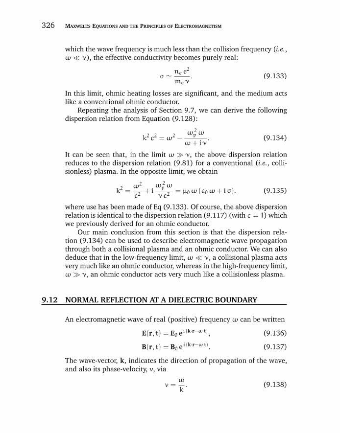
“chapter9” — 2007/11/30 — 11:11 — page 326 — #28
326 MAXWELL’S EQUATIONS AND THE PRINCIPLES OF ELECTROMAGNETISM
which the wave frequency is much less than the collision frequency (i.e.,ω ν), the effective conductivity becomes purely real:
σ ne e2
me ν. (9.133)
In this limit, ohmic heating losses are significant, and the medium actslike a conventional ohmic conductor.
Repeating the analysis of Section 9.7, we can derive the followingdispersion relation from Equation (9.128):
k2 c2 = ω2 −ω2p ω
ω+ iν. (9.134)
It can be seen that, in the limit ω ν, the above dispersion relationreduces to the dispersion relation (9.81) for a conventional (i.e., colli-sionless) plasma. In the opposite limit, we obtain
k2 =ω2
c2+ i
ω2p ω
νc2= µ0 ω (ε0 ω+ iσ). (9.135)
where use has been made of Eq (9.133). Of course, the above dispersionrelation is identical to the dispersion relation (9.117) (with ε = 1) whichwe previously derived for an ohmic conductor.
Our main conclusion from this section is that the dispersion rela-tion (9.134) can be used to describe electromagnetic wave propagationthrough both a collisional plasma and an ohmic conductor. We can alsodeduce that in the low-frequency limit, ω ν, a collisional plasma actsvery much like an ohmic conductor, whereas in the high-frequency limit,ω ν, an ohmic conductor acts very much like a collisionless plasma.
9.12 NORMAL REFLECTION AT A DIELECTRIC BOUNDARY
An electromagnetic wave of real (positive) frequency ω can be written
E(r, t) = E0 e i (k·r−ωt), (9.136)
B(r, t) = B0 e i (k·r−ωt). (9.137)
The wave-vector, k, indicates the direction of propagation of the wave,and also its phase-velocity, v, via
v =ω
k. (9.138)
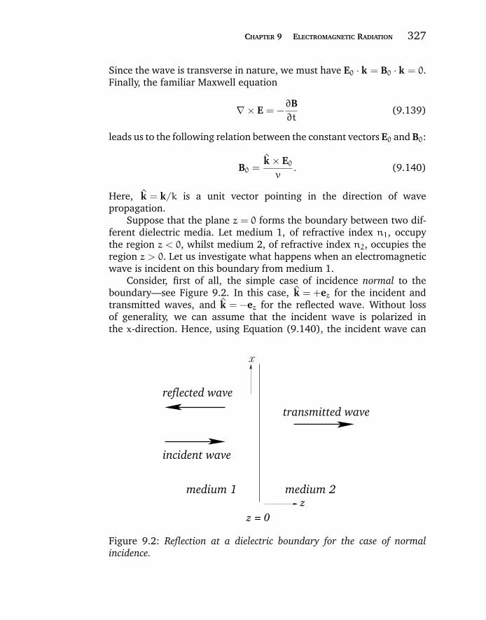
“chapter9” — 2007/11/30 — 11:11 — page 327 — #29
CHAPTER 9 ELECTROMAGNETIC RADIATION 327
Since the wave is transverse in nature, we must have E0 · k = B0 · k = 0.Finally, the familiar Maxwell equation
∇ × E = −∂B∂t
(9.139)
leads us to the following relation between the constant vectors E0 and B0:
B0 =k × E0v
. (9.140)
Here, k = k/k is a unit vector pointing in the direction of wavepropagation.
Suppose that the plane z = 0 forms the boundary between two dif-ferent dielectric media. Let medium 1, of refractive index n1, occupythe region z < 0, whilst medium 2, of refractive index n2, occupies theregion z > 0. Let us investigate what happens when an electromagneticwave is incident on this boundary from medium 1.
Consider, first of all, the simple case of incidence normal to theboundary—see Figure 9.2. In this case, k = +ez for the incident andtransmitted waves, and k = −ez for the reflected wave. Without lossof generality, we can assume that the incident wave is polarized inthe x-direction. Hence, using Equation (9.140), the incident wave can
zz = 0
medium 1
reflected wave
incident wave
x
transmitted wave
medium 2
Figure 9.2: Reflection at a dielectric boundary for the case of normalincidence.

“chapter9” — 2007/11/30 — 11:11 — page 328 — #30
328 MAXWELL’S EQUATIONS AND THE PRINCIPLES OF ELECTROMAGNETISM
be written
E(z, t) = Ei e i (k1 z−ωt) ex, (9.141)
B(z, t) =Ei
v1e i (k1 z−ωt) ey, (9.142)
where v1 = c/n1 is the phase-velocity in medium 1, and k1 = ω/v1.Likewise, the reflected wave takes the form
E(z, t) = Er e i (−k1 z−ωt) ex, (9.143)
B(z, t) = −Er
v1e i (−k1 z−ωt) ey. (9.144)
Finally, the transmitted wave can be written
E(z, t) = Et e i (k2 z−ωt) ex, (9.145)
B(z, t) =Et
v2e i (k2 z−ωt) ey, (9.146)
where v2 = c/n2 is the phase-velocity in medium 2, and k2 = ω/v2.For the case of normal incidence, the electric and magnetic compo-
nents of all three waves are parallel to the boundary between the twodielectric media. Hence, the appropriate boundary conditions to applyat z = 0 are
E‖ 1 = E‖ 2, (9.147)
B‖ 1 = B‖ 2. (9.148)
The latter condition derives from the general boundary condition H‖ 1 =H‖ 2, and the fact that B = µ0 H in both media (which are assumed to benon-magnetic).
Application of the boundary condition (9.147) yields
Ei + Er = Et. (9.149)
Likewise, application of the boundary condition (9.148) gives
Ei − Er
v1=Et
v2, (9.150)
or
Ei − Er =v1
v2Et =
n2
n1Et, (9.151)
“chapter9” — 2007/11/30 — 11:11 — page 329 — #31
CHAPTER 9 ELECTROMAGNETIC RADIATION 329
since v1/v2 = n2/n1. Equations (9.149) and (9.151) can be solved togive
Er =
(n1 − n2n1 + n2
)Ei, (9.152)
Et =
(2n1
n1 + n2
)Et. (9.153)
Thus, we have determined the amplitudes of the reflected and transmit-ted waves in terms of the amplitude of the incident wave.
It can be seen, first of all, that if n1 = n2 then Er = 0 and Et = Ei. Inother words, if the two media have the same indices of refraction thenthere is no reflection at the boundary between them, and the transmit-ted wave is consequently equal in amplitude to the incident wave. Onthe other hand, if n1 = n2 then there is some reflection at the boundary.Indeed, the amplitude of the reflected wave is roughly proportional tothe difference between n1 and n2. This has important practical conse-quences. We can only see a clean pane of glass in a window becausesome of the light incident on an air/glass boundary is reflected, dueto the different refractive indicies of air and glass. As is well-known, itis a lot more difficult to see glass when it is submerged in water. Thisis because the refractive indices of glass and water are quite similar,and so there is very little reflection of light incident on a water/glassboundary.
According to Equation (9.152), Er/Ei < 0 when n2 > n1. The nega-tive sign indicates a 180 phase-shift of the reflected wave, with respectto the incident wave. We conclude that there is a 180 phase-shift ofthe reflected wave, relative to the incident wave, on reflection from aboundary with a medium of greater refractive index. Conversely, thereis no phase-shift on reflection from a boundary with a medium of lesserrefractive index.
The mean electromagnetic energy flux, or intensity, in the z-directionis simply
I =〈E × B · ez〉
µ0=E0 B0
2 µ0=
E202 µ0 v
. (9.154)
The coefficient of reflection, R, is defined as the ratio of the intensities ofthe reflected and incident waves:
R =Ir
Ii=
(Er
Ei
)2. (9.155)
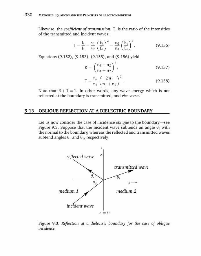
“chapter9” — 2007/11/30 — 11:11 — page 330 — #32
330 MAXWELL’S EQUATIONS AND THE PRINCIPLES OF ELECTROMAGNETISM
Likewise, the coefficient of transmission, T , is the ratio of the intensitiesof the transmitted and incident waves:
T =It
Ii=v1
v2
(Et
Ei
)2=n2
n1
(Et
Ei
)2. (9.156)
Equations (9.152), (9.153), (9.155), and (9.156) yield
R =
(n1 − n2n1 + n2
)2, (9.157)
T =n2
n1
(2n1
n1 + n2
)2. (9.158)
Note that R+ T = 1. In other words, any wave energy which is notreflected at the boundary is transmitted, and vice versa.
9.13 OBLIQUE REFLECTION AT A DIELECTRIC BOUNDARY
Let us now consider the case of incidence oblique to the boundary—seeFigure 9.3. Suppose that the incident wave subtends an angle θi withthe normal to the boundary, whereas the reflected and transmitted wavessubtend angles θr and θt, respectively.
z
x
transmitted wave
medium 2
incident wave
medium 1
reflected wave
z = 0
θr θt
θi
Figure 9.3: Reflection at a dielectric boundary for the case of obliqueincidence.
“chapter9” — 2007/11/30 — 11:11 — page 331 — #33
CHAPTER 9 ELECTROMAGNETIC RADIATION 331
The incident wave can be written
E(r, t) = Ei e i (ki·r−ωt), (9.159)
B(r, t) = Bi e i (ki·r−ωt), (9.160)
with analogous expressions for the reflected and transmitted waves.Since, in the case of oblique incidence, the electric and magnetic com-ponents of the wave fields are no longer necessarily parallel to theboundary, the boundary conditions (9.147) and (9.148) at z = 0 mustbe supplemented by the additional boundary conditions
ε1 E⊥ 1 = ε2 E⊥ 2, (9.161)
B⊥ 1 = B⊥ 2. (9.162)
Equation (9.161) derives from the general boundary conditionD⊥ 1 = D⊥ 2.
It follows from Equations (9.148) and (9.162) that both componentsof the magnetic field are continuous at the boundary. Hence, we can write
Bi e i (ki·r−ωt) + Br e i (kr·r−ωt) = Bt e i (kt·r−ωt) (9.163)
at z = 0. Given that Bi, Br, and Bt are constant vectors, the only way inwhich the above equation can be satisfied for all values of x and y is if
ki · r = kr · r = kt · r (9.164)
throughout the z = 0 plane. This, in turn, implies that
ki x = kr x = kt x (9.165)
and
ki y = kry = kty. (9.166)
It immediately follows that if ki y = 0 then kry = kty = 0. In other words,if the incident wave lies in the x-z plane then the reflected and transmit-ted waves also lie in the x-z plane. Another way of putting this is thatthe incident, reflected, and transmitted waves all lie in the same plane,known as the plane of incidence. This, of course, is one of the laws of geo-metric optics. From now on, we shall assume that the plane of incidenceis the x-z plane.
Now, ki = kr = ω/v1 and kt = ω/v2. Moreover,
sin θi =kx i
ki, (9.167)
“chapter9” — 2007/11/30 — 11:11 — page 332 — #34
332 MAXWELL’S EQUATIONS AND THE PRINCIPLES OF ELECTROMAGNETISM
with similar expressions for θr and θt. Hence, according to Equation(9.165),
sin θr = sin θi, (9.168)
which implies that θr = θi. Moreover,
sin θtsin θi
=v2
v1=n1
n2. (9.169)
Of course, the above expressions correspond to the law of reflection andSnell’s law of refraction, respectively.
For the case of oblique incidence, we need to consider two inde-pendent wave polarizations separately. The first polarization has all thewave electric fields parallel to the boundary whilst the second has all thewave magnetic fields parallel to the boundary.
Let us consider the first wave polarization. We can write unit vec-tors in the directions of propagation of the incident, reflected, andtransmitted waves like so:
ki = (sin θi, 0, cos θi) , (9.170)
kr = (sin θi, 0, − cos θi) , (9.171)
kt = (sin θt, 0, cos θt) . (9.172)
The constant vectors associated with the incident wave are written
Ei = Ei ey, (9.173)
Bi =Ei
v1(− cos θi, 0, sin θi) , (9.174)
where use has been made of Equation (9.140). Likewise, the constantvectors associated with the reflected and transmitted waves are
Er = Er ey, (9.175)
Br =Er
v1(cos θi, 0, sin θi) , (9.176)
and
Et = Et ey, (9.177)
Bt =Et
v2(− cos θt, 0, sin θt) , (9.178)
respectively.
“chapter9” — 2007/11/30 — 11:11 — page 333 — #35
CHAPTER 9 ELECTROMAGNETIC RADIATION 333
Now, the boundary condition (9.147) yields Ey1 = Ey2, or
Ei + Er = Et. (9.179)
Likewise, the boundary condition (9.162) gives Bz1 = Bz2, or
(Ei + Er)sin θiv1
= Etsin θtv2
. (9.180)
However, using Snell’s law, (9.169), the above expression reduces toEquation (9.179). Finally, the boundary condition (9.148) yields Bx1 =Bx2, or
(Ei − Er)cos θiv1
= Etcos θtv2
. (9.181)
It is convenient to define the parameters
α =cos θtcos θi
, (9.182)
and
β =v1
v2=n2
n1. (9.183)
Equations (9.179) and (9.181) can be solved in terms of these parame-ters to give
Er =
(1− αβ
1+ αβ
)Ei, (9.184)
Et =
(2
1+ αβ
)Ei. (9.185)
These relations are known as Fresnel equations.The wave intensity in the z-direction is given by
Iz =〈E × B · ez〉
µ0=E0 B0 cos θ2µ0
=E20 cos θ2µ0 v
. (9.186)
Hence, the coefficient of reflection is written
R =
(Er
Ei
)2=
(1− αβ
1+ αβ
)2, (9.187)
whereas the coefficient of transmission takes the form
T =cos θtcos θi
v1
v2
(Et
Ei
)2= αβ
(2
1+ αβ
)2. (9.188)
Note that it is again the case that R+ T = 1.
“chapter9” — 2007/11/30 — 11:11 — page 334 — #36
334 MAXWELL’S EQUATIONS AND THE PRINCIPLES OF ELECTROMAGNETISM
Let us now consider the second wave polarization. In this case, theconstant vectors associated with the incident, reflected, and transmittedwaves are written
Ei = Ei (cos θi, 0, − sin θi), (9.189)
Bi =Ei
v1ey, (9.190)
and
Er = Er (cos θi, 0, sin θi), (9.191)
Br = −Er
v1ey, (9.192)
and
Et = Et (cos θt, 0, − sin θt), (9.193)
Bt =Et
v2ey, (9.194)
respectively. The boundary condition (9.148) yields By1 = By2, or
Ei − Er
v1=Et
v2. (9.195)
Likewise, the boundary condition (9.147) gives Ex 1 = Ex 2, or
(Ei + Er) cos θi = Et cos θt. (9.196)
Finally, the boundary condition (9.161) yields ε1 Ez 1 = ε2 Ez 2, or
ε1 (Ei − Er) sin θi = ε2 Ei sin θt. (9.197)
Making use of Snell’s law, and the fact that ε = n2, the above expressionreduces to Equation (9.195).
Solving Equations (9.165) and (9.196), we obtain
Er =
(α− β
α+ β
)Ei, (9.198)
Et =
(2
α+ β
)Ei. (9.199)
The associated coefficients of reflection and transmission take the form
R =
(α− β
α+ β
)2, (9.200)
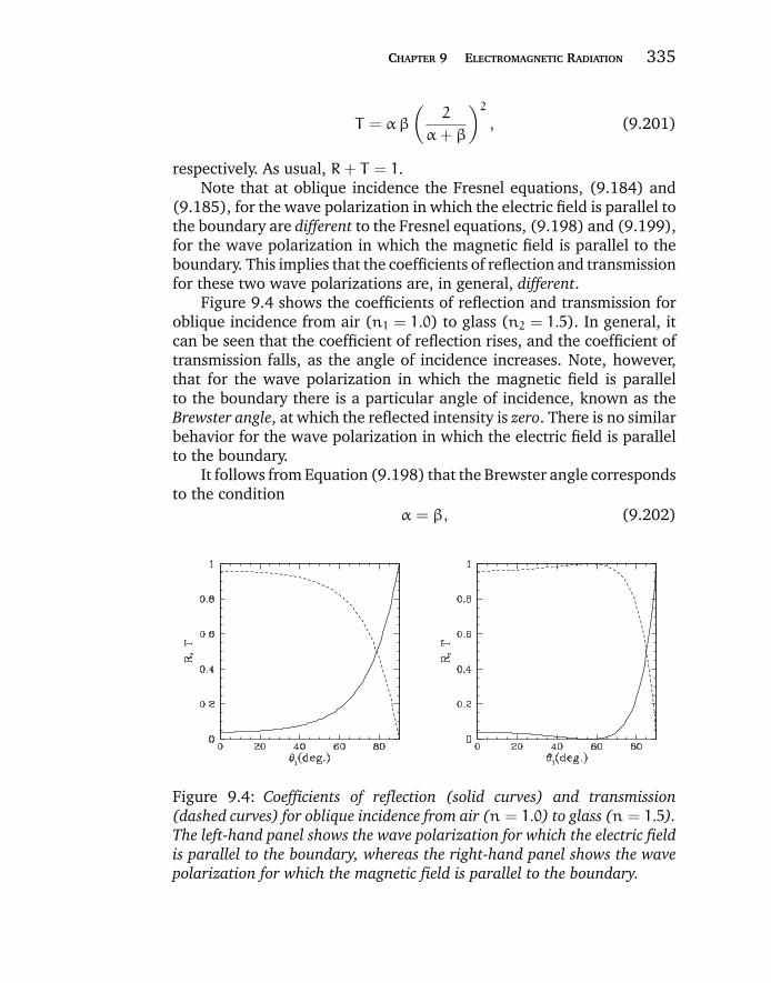
“chapter9” — 2007/11/30 — 11:11 — page 335 — #37
CHAPTER 9 ELECTROMAGNETIC RADIATION 335
T = αβ
(2
α+ β
)2, (9.201)
respectively. As usual, R+ T = 1.Note that at oblique incidence the Fresnel equations, (9.184) and
(9.185), for the wave polarization in which the electric field is parallel tothe boundary are different to the Fresnel equations, (9.198) and (9.199),for the wave polarization in which the magnetic field is parallel to theboundary. This implies that the coefficients of reflection and transmissionfor these two wave polarizations are, in general, different.
Figure 9.4 shows the coefficients of reflection and transmission foroblique incidence from air (n1 = 1.0) to glass (n2 = 1.5). In general, itcan be seen that the coefficient of reflection rises, and the coefficient oftransmission falls, as the angle of incidence increases. Note, however,that for the wave polarization in which the magnetic field is parallelto the boundary there is a particular angle of incidence, known as theBrewster angle, at which the reflected intensity is zero. There is no similarbehavior for the wave polarization in which the electric field is parallelto the boundary.
It follows from Equation (9.198) that the Brewster angle correspondsto the condition
α = β, (9.202)
Figure 9.4: Coefficients of reflection (solid curves) and transmission(dashed curves) for oblique incidence from air (n = 1.0) to glass (n = 1.5).The left-hand panel shows the wave polarization for which the electric fieldis parallel to the boundary, whereas the right-hand panel shows the wavepolarization for which the magnetic field is parallel to the boundary.
“chapter9” — 2007/11/30 — 11:11 — page 336 — #38
336 MAXWELL’S EQUATIONS AND THE PRINCIPLES OF ELECTROMAGNETISM
or
β2 =cos2 θtcos2 θi
=1− sin2 θt1− sin2 θi
=1− sin2 θi/β2
1− sin2 θi, (9.203)
where use has been made of Snell’s law. The above expression reduces to
sin θi =β√1+ β2
, (9.204)
or tan θi = β = n2/n1. Hence, the Brewster angle satisfies
θB = tan−1
(n2
n1
). (9.205)
If unpolarized light is incident on an air/glass (say) boundary at theBrewster angle then the reflected light is 100% plane polarized.
9.14 TOTAL INTERNAL REFLECTION
Let us again consider an electromagnetic wave obliquely incident ona dielectric boundary. According to Equation (9.169), the angle ofrefraction θt is related to the angle of incidence θi via
sin θt =n1
n2sin θi. (9.206)
This formula presents no problems when n1 < n2. However, if n1 > n2then the formula predicts that sin θt is greater than unity when the angleof incidence exceeds some critical angle given by
θc = sin−1(n2/n1). (9.207)
Obviously, in this situation, we can no longer interpret sin θt as the sine ofan angle. Moreover, cos θt ≡ (1− sin2 θt)1/2 can no longer be interpretedas the cosine of an angle. However, these quantities still specify thewave-vector of the transmitted wave. In fact, from Equation (9.172),
kt = kt (sin θt, 0, i cos θt), (9.208)
where kt = n2 ω/c, cos θt = (sin2 θt − 1)1/2, and
sin θt =sin θisin θc
. (9.209)
“chapter9” — 2007/11/30 — 11:11 — page 337 — #39
CHAPTER 9 ELECTROMAGNETIC RADIATION 337
Here, the hat on θt is to remind us that this quantity is not a real angle.Now, the transmitted wave varies as
e i (kt·r−ωt) = e−kt cos θt e i (kt sin θt−ωt). (9.210)
Hence, we conclude that when θi > θc the transmitted wave is evanes-cent: i.e., it decays exponentially, rather than propagating, in medium 2.
When θi > θc the parameter α, defined in Equation (9.182),becomes complex. In fact, α → i α, where
α =cos θtcos θi
. (9.211)
Note that the parameter β, defined in Eq. (9.183), remains real. Hence,from Equations (9.184) and (9.198), the relationship between Er and Eifor the two previously discussed wave polarizations, in which either theelectric field or the magnetic field is parallel to the boundary, are
Er =
(1− i α β1+ i α β
)Ei, (9.212)
Er =
(i α− β
i α+ β
)Ei, (9.213)
respectively. In both cases, the associated coefficients of reflection areunity: i.e.,
R =
∣∣∣∣ErEi∣∣∣∣2
= 1. (9.214)
In other words, the incident wave undergoes complete reflection at theboundary. This phenomenon is called total internal reflection, and occurswhenever a wave is incident on a boundary separating a medium of highrefractive index from a medium of low refractive index, and the angleof incidence exceeds the critical angle, θc.
Figure 9.5 shows the coefficients of reflection and transmission foroblique incidence from water (n1 = 1.33) to air (n2 = 1.0). In this case,the critical angle is θc = 48.8.
Note that when total internal reflection takes place the evanescenttransmitted wave penetrates a few wavelengths into the lower refractiveindex medium, since (as is easily demonstrated) the amplitude of thiswave is non-zero. The existence of the evanescent wave can be demon-strated using the apparatus pictured in Figure 9.6. Here, we have tworight-angled glass prisms separated by a small air gap of width d. Light

“chapter9” — 2007/11/30 — 11:11 — page 338 — #40
338 MAXWELL’S EQUATIONS AND THE PRINCIPLES OF ELECTROMAGNETISM
Figure 9.5: Coefficients of reflection (solid curves) and transmission(dashed curves) for oblique incidence from water (n = 1.33) to air(n = 1.0). The left-hand panel shows the wave polarization for whichthe electric field is parallel to the boundary, whereas the right-hand panelshows the wave polarization for which the magnetic field is parallel to theboundary.
transmitted
d
air
incident
glass prisms
reflected
Figure 9.6: Frustrated total internal reflection.
incident on the internal surface of the first prism is internally reflected(assuming that θc < 45). However, if the spacing d is not too muchlarger than the wavelength of the light (in air) then the evanescent wavein the air gap still has a finite amplitude when it reaches the second prism.In this case, a detectable transmitted wave is excited in the second prism.
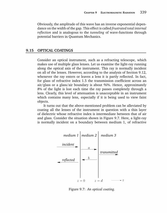
“chapter9” — 2007/11/30 — 11:11 — page 339 — #41
CHAPTER 9 ELECTROMAGNETIC RADIATION 339
Obviously, the amplitude of this wave has an inverse exponential depen-dance on the width of the gap. This effect is called frustrated total internalreflection and is analogous to the tunneling of wave-functions throughpotential barriers in Quantum Mechanics.
9.15 OPTICAL COATINGS
Consider an optical instrument, such as a refracting telescope, whichmakes use of multiple glass lenses. Let us examine the light-ray runningalong the optical axis of the instrument. This ray is normally incidenton all of the lenses. However, according to the analysis of Section 9.12,whenever the ray enters or leaves a lens it is partly reflected. In fact,for glass of refractive index 1.5 the transmission coefficient across anair/glass or a glass/air boundary is about 96%. Hence, approximately8% of the light is lost each time the ray passes completely through alens. Clearly, this level of attenuation is unacceptable in an instrumentwhich contains many lens, especially if it is being used to view faintobjects.
It turns out that the above-mentioned problem can be alleviated bycoating all the lenses of the instrument in question with a thin layerof dielectric whose refractive index is intermediate between that of airand glass. Consider the situation shown in Figure 9.7. Here, a light-rayis normally incident on a boundary between medium 1, of refractive
b
zz = dz = 0
medium 1
incident
reflected
medium 2 medium 3
transmitteda
Figure 9.7: An optical coating.
“chapter9” — 2007/11/30 — 11:11 — page 340 — #42
340 MAXWELL’S EQUATIONS AND THE PRINCIPLES OF ELECTROMAGNETISM
index n1, and medium 3, of refractive index n3. Here, medium 1 repre-sents air, and medium 3 represents glass, or vice versa. Suppose that theglass is covered with a thin optical coating, referred to as medium 2, ofthickness d, and refractive index n2.
In the notation of Section 9.12, the incident wave is written
E(z, t) = Ei e i (k1 z−ωt) ex, (9.215)
B(z, t) =Ei
v1e i (k1 z−ωt) ey, (9.216)
where v1 = c/n1 is the phase-velocity in medium 1, and k1 = ω/v1.Likewise, the reflected wave takes the form
E(z, t) = Er e i (−k1 z−ωt) ex, (9.217)
B(z, t) = −Er
v1e i (−k1 z−ωt) ey. (9.218)
The wave traveling to the right in medium 2 is written
E(z, t) = Ea e i (k2 z−ωt) ex, (9.219)
B(z, t) =Ea
v2e i (k2 z−ωt) ey, (9.220)
where v2 = c/n2 is the phase-velocity in medium 2, and k2 = ω/v2.Likewise, the wave traveling to the left takes the form
E(z, t) = Eb e i (−k2 z−ωt) ex, (9.221)
B(z, t) = −Eb
v2e i (−k2 z−ωt) ey. (9.222)
Finally, the transmitted wave is written
E(z, t) = Et e i [k3 (z−d)−ωt] ex, (9.223)
B(z, t) =Et
v3e i [k2 (z−d)−ωt] ey, (9.224)
where v3 = c/n3 is the phase-velocity in medium 3, and k3 = ω/v3.Continuity of Ex and By at z = 0 yield
Ei + Er = Ea + Eb, (9.225)Ei − Er
v1= =
Ea − Ebv2
, (9.226)
“chapter9” — 2007/11/30 — 11:11 — page 341 — #43
CHAPTER 9 ELECTROMAGNETIC RADIATION 341
respectively, whereas continuity of Ex and By at z = d give
Ea e i k2 d + Eb e−i k2 d = Et, (9.227)
Ea e i k2 d − Eb e−i k2 d
v2=Et
v3, (9.228)
respectively. At this point, it is convenient to make the special choicek2 d = π/2. This corresponds to the optical coating being exactly one-quarter of a wavelength thick. It follows that
Ea − Eb = − iEt, (9.229)
Ea + Eb = − in3
n2Et. (9.230)
The above equations can be solved to give
Er = −
(1− α
1+ α
)Ei, (9.231)
Et =n1
n2
2 i1+ α
Ei, (9.232)
where
α =n1 n3
n22. (9.233)
Thus, the overall coefficient of reflection is
R =
∣∣∣∣ErEi∣∣∣∣2
=
(1− α
1+ α
)2, (9.234)
whereas the overall coefficient of transmission is
T =n3
n1
∣∣∣∣EtEi∣∣∣∣2
=4α
(1+ α)2. (9.235)
Suppose finally that
n2 =√n1 n3 : (9.236)
i.e., the refractive index of the coating is the geometric mean of that ofair and glass. In this case, α = 1, and it follows from Equations (9.234)and (9.235) that there is zero reflection, and 100% transmission, atthe boundary. Hence, by coating lenses with a one-quarter wavelengththickness of a substance whose refractive index is (approximately) thegeometric mean between those of air and glass (e.g., Magnesium flu-oride, whose refractive index is 1.38), we can completely eliminate
“chapter9” — 2007/11/30 — 11:11 — page 342 — #44
342 MAXWELL’S EQUATIONS AND THE PRINCIPLES OF ELECTROMAGNETISM
unwanted reflections. This technique is widely used in high-quality opti-cal instruments. Note that the physics of quarter-wavelength optical coat-ings is analogous to that of quarter-wave transformers in transmissionlines—see Section 7.7.
9.16 REFLECTION AT A METALLIC BOUNDARY
Let us now consider the reflection of electromagnetic radiation by ametallic surface. This investigation is obviously relevant to optical instru-ments, such as reflecting telescopes, which make use of mirrors. For thesake of simplicity, we shall restrict our investigation to the case of normalincidence.
A metal is, by definition, a good electrical conductor. According toEquation (9.121), the wave-number of an electromagnetic wave of fre-quency ω in a good conductor of conductivity σ (and true dielectricconstant unity) is
k √
iµ0 σω. (9.237)
Hence, it follows that the effective refractive index of the conductor is
n =k c
ω√
iσε0 ω
. (9.238)
Note that the good conductor ordering σ ε0 ω ensures that |n| 1.For the case of a light-ray in air reflecting at normal incidence off
a metal mirror, we can employ the previously derived formula (9.152)with n1 = 1 and n2 = n, where n is specified above. We obtain
Er
Ei=1− n
1+ n −1+
2
n, (9.239)
where we have made use of the fact that |n| 1. Hence, the coefficientof reflection of the mirror takes the form
R =
∣∣∣∣ErEi∣∣∣∣2
1− Re(4
n
), (9.240)
or
R 1−
√8 ε0 ω
σ. (9.241)
High-quality metallic mirrors are generally coated in Silver, whoseconductivity is 6.3× 10⁷ (Ωm)−1. It follows, from the above formula,
“chapter9” — 2007/11/30 — 11:11 — page 343 — #45
CHAPTER 9 ELECTROMAGNETIC RADIATION 343
that at optical frequencies (ω = 4× 10¹⁵ rad./s) the coefficient of reflec-tion of a silvered mirror is R 93.3%. This implies that about 7% ofthe light incident on a silvered mirror is absorbed, rather than beingreflected. This rather severe light loss can be problematic in instruments,such as astronomical telescopes, which are used to view faint objects.
9.17 WAVE-GUIDES
A wave-guide is a hollow conducting pipe, of uniform cross-section,used to transport high-frequency electromagnetic waves (generally, inthe microwave band) from one point to another. The main advantageof wave-guides is their relatively low level of radiation losses (since theelectric and magnetic fields are completely enclosed by a conductingwall) compared to transmission lines.
Consider a vacuum-filled wave-guide which runs parallel to the z-axis. An electromagnetic wave trapped inside the wave-guide satisfiesMaxwell’s equations for free space:
∇ · E = 0, (9.242)
∇ · B = 0, (9.243)
∇ × E = −∂B∂t, (9.244)
∇ × B =1
c2∂E∂t. (9.245)
Let ∂/∂t ≡ −iω, and ∂/∂z ≡ i k, where ω is the wave frequency, and kthe wave-number parallel to the axis of the wave-guide. It follows that
∂Ex
∂x+∂Ey
∂y+ i kEz = 0, (9.246)
∂Bx
∂x+∂By
∂y+ i kBz = 0, (9.247)
iωBx =∂Ez
∂y− i kEy, (9.248)
iωBy = −∂Ez
∂x+ i kEx, (9.249)
iωBz =∂Ey
∂x−∂Ex
∂y, (9.250)

“chapter9” — 2007/11/30 — 11:11 — page 344 — #46
344 MAXWELL’S EQUATIONS AND THE PRINCIPLES OF ELECTROMAGNETISM
iω
c2Ex = −
∂Bz
∂y+ i kBy, (9.251)
iω
c2Ey =
∂Bz
∂x− i kBx, (9.252)
iω
c2Ez = −
∂By
∂x+∂Bx
∂y. (9.253)
Equations (9.249) and (9.251) yield
Ex = i(ω∂Bz
∂y+ k
∂Ez
∂x
)(ω2
c2− k2
)−1
, (9.254)
and
By = i(ω
c2∂Ez
∂x+ k
∂Bz
∂y
)(ω2
c2− k2
)−1
. (9.255)
Likewise, Equations (9.248) and (9.252) yield
Ey = i(
−ω∂Bz
∂x+ k
∂Ez
∂y
)(ω2
c2− k2
)−1
, (9.256)
and
Bx = i(
−ω
c2∂Ez
∂y+ k
∂Bz
∂x
)(ω2
c2− k2
)−1
. (9.257)
These equations can be combined to give
Et = i (ω∇Bz × ez + k∇Ez)(ω2
c2− k2
)−1
, (9.258)
Bt = i(−ω
c2∇Ez × ez + k∇Bz
)(ω2c2
− k2)−1
. (9.259)
Here, Et and Bt are the transverse electric and magnetic fields: i.e., theelectric and magnetic fields in the x-y plane. It is clear, from Equa-tions (9.258) and (9.259), that the transverse fields are fully determinedonce the longitudinal fields, Ez and Bz, are known.
Substitution of Equations (9.258) and (9.259) into Equations(9.250) and (9.253) yields the equations satisfied by the longitudinal
“chapter9” — 2007/11/30 — 11:11 — page 345 — #47
CHAPTER 9 ELECTROMAGNETIC RADIATION 345
fields: (∂2
∂x2+∂2
∂y2
)Ez +
(ω2
c2− k2
)Ez = 0, (9.260)
(∂2
∂x2+∂2
∂y2
)Bz +
(ω2
c2− k2
)Bz = 0. (9.261)
The remaining equations, (9.246) and (9.247), are automaticallysatisfied provided Equations (9.258)–(9.261) are satisfied.
We expect E = B = 0 inside the walls of the wave-guide, assumingthat they are perfectly conducting. Hence, the appropriate boundaryconditions at the walls are
E‖ = 0, (9.262)
B⊥ = 0. (9.263)
It follows, by inspection of Equations (9.258) and (9.259), that theseboundary conditions are satisfied provided
Ez = 0, (9.264)
n · ∇Bz = 0, (9.265)
at the walls. Here, n is a unit vector normal to the walls. Hence, theelectromagnetic fields inside the wave-guide are fully specified by solv-ing Equations (9.260) and (9.261), subject to the boundary conditions(9.264) and (9.265), respectively.
Equations (9.260) and (9.261) support two independent types ofsolution. The first type has Ez = 0, and is consequently called a transverseelectric, or TE, mode. Conversely, the second type has Bz = 0, and iscalled a transverse magnetic, or TM, mode.
Consider the specific example of a rectangular wave-guide, with con-ducting walls at x = 0, a, and y = 0, b. For a TE mode, the longitudinalmagnetic field can be written
Bz(x, y) = B0 cos(kx x) cos(ky y). (9.266)
The boundary condition (9.265) requires that ∂Bz/∂x = 0 at x = 0, a,and ∂Bz/∂y = 0 at y = 0, b. It follows that
kx =mπ
a, (9.267)
ky =nπ
b, (9.268)
“chapter9” — 2007/11/30 — 11:11 — page 346 — #48
346 MAXWELL’S EQUATIONS AND THE PRINCIPLES OF ELECTROMAGNETISM
where m = 0, 1, 2, · · · , and n = 0, 1, 2, · · · . Clearly, there are many dif-ferent kinds of TE mode, corresponding to the many different choicesof m and n. Let us refer to a mode corresponding to a particular choiceof m,n as a TEmn mode. Note, however, that there is no TE00 mode,since Bz(x, y) is uniform in this case. According to Equation (9.261), thedispersion relation for the TEmn mode is given by
k2 c2 = ω2 −ω2mn, (9.269)
where
ωmn = c π
√m2
a2+n2
b2. (9.270)
According to the dispersion relation (9.269), k is imaginary forω < ωmn. In other words, for wave frequencies below ωmn, the TEmnmode fails to propagate down the wave-guide, and is instead attenuated.Hence,ωmn is termed the cut-off frequency for the TEmn mode. Assumingthat a > b, the TE mode with the lowest cut-off frequency is the TE10mode, where
ω10 =c π
a. (9.271)
For frequencies above the cut-off frequency, the phase-velocity of theTEmn mode is given by
vp =ω
k=
c√1−ω2
mn/ω2, (9.272)
which is greater than c. However, the group-velocity takes the form
vg =dω
dk= c
√1−ω2
mn/ω2, (9.273)
which is always less than c. Of course, energy is transmitted down thewave-guide at the group-velocity, rather than the phase-velocity. Notethat the group-velocity goes to zero as the wave frequency approachesthe cut-off frequency.
For a TM mode, the longitudinal electric field can be written
Ez(x, y) = E0 sin(kx x) sin(ky y). (9.274)
The boundary condition (9.264) requires that Ez = 0 at x = 0, a, andy = 0, b. It follows that
kx =mπ
a, (9.275)
ky =nπ
b, (9.276)
“chapter9” — 2007/11/30 — 11:11 — page 347 — #49
CHAPTER 9 ELECTROMAGNETIC RADIATION 347
where m = 1, 2, · · · , and n = 1, 2, · · · . The dispersion relation for theTMmn mode is also given by Equation (9.269). Hence, Equations (9.272)and (9.273) also apply to TM modes. However, the TM mode with thelowest cut-off frequency is the TM11 mode, where
ω11 = c π
√1
a2+1
b2> ω10. (9.277)
It follows that the mode with the lowest cut-off frequency is always a TEmode.
There is, in principle, a third type of mode which can propagate downa wave-guide. This third mode type is characterized by Ez = Bz = 0, andis consequently called a transverse electromagnetic, or TEM, mode. It iseasily seen, from an inspection of Equations (9.248)–(9.253), that a TEMmode satisfies
ω2 = k2 c2, (9.278)
and
Et = − ∇φ, (9.279)
Bt = c−1∇φ× ez, (9.280)
where φ(x, y) satisfies
∇2φ = 0. (9.281)
The boundary conditions (9.264) and (9.265) imply that
φ = constant (9.282)
at the walls. However, there is no non-trivial solution of Equa-tions (9.281) and (9.282) for a conventional wave-guide. In other words,conventional wave-guides do not support TEM modes. It turns out thatonly wave-guides with central conductors support TEM modes. Consider,for instance, a coaxial wave-guide in which the electric and magneticfields are trapped between two coaxial cylindrical conductors of radiusa and b (with b > a). In this case, φ = φ(r), and Equation (9.281)reduces to
1
r
∂
∂r
(r∂φ
∂r
)= 0, (9.283)
where r is a standard cylindrical polar coordinate. The boundary con-dition (9.282) is automatically satisfied at r = a and r = b. The above
“chapter9” — 2007/11/30 — 11:11 — page 348 — #50
348 MAXWELL’S EQUATIONS AND THE PRINCIPLES OF ELECTROMAGNETISM
equation has the following non-trivial solution:
φ(r) = φb ln(r/b). (9.284)
Note, however, that the inner conductor must be present, otherwiseφ →∞ as r → 0, which is unphysical. According to the dispersion relation(9.278), TEM modes have no cut-off frequency, and have the phase-velocity (and group-velocity) c. Indeed, this type of mode is the same asthat supported by a transmission line (see Section 7.7).
9.18 EXERCISES
9.1. Consider an electromagnetic wave propagating through a non-dielectric, non-
magnetic medium containing free charge density ρ and free current density j.
Demonstrate from Maxwell’s equations that the associated wave equations take
the form
∇2E −1
c2∂2E∂t2
=∇ρε0
+ µ0∂j∂t,
∇2B −1
c2∂2B∂t2
= −µ0 ∇ × j.
9.2. A spherically symmetric charge distribution undergoes purely radial oscillations.
Show that no electromagnetic waves are emitted. [Hint: Show that there is no
magnetic field.]
9.3. A general electromagnetic wave-pulse propagating in the z-direction at velocity
u is written
E = P(z − u t) ex +Q(z − u t) ey + R(z − u t) ez,
B =S(z − u t)
uex +
T(z − u t)
uey +
U(z − u t)
uez,
where P, Q, R, S, T , and U are arbitrary functions. In order to exclude electro-
static and magnetostatic fields, these functions are subject to the constraint that
〈P〉 = 〈Q〉 = 〈R〉 = 〈S〉 = 〈T〉 = 〈U〉 = 0, where
〈P〉 =
∫∞
−∞
P(x)dx.
Suppose that the pulse propagates through a uniform dielectric medium of
dielectric constant ε. Demonstrate from Maxwell’s equation that u = c/√ε,
R = U = 0, S = −Q, and T = P. Incidentally, this result implies that a general
wave-pulse is characterized by two arbitrary functions, corresponding to the two
possible independent polarizations of the pulse.
“chapter9” — 2007/11/30 — 11:11 — page 349 — #51
CHAPTER 9 ELECTROMAGNETIC RADIATION 349
9.4. A medium is such that the product of the phase and group velocities of elec-
tromagnetic waves is equal to c2 at all wave frequencies. Demonstrate that the
dispersion relation for electromagnetic waves takes the form
ω2 = k
2c2 +ω2
0 ,
where ω0 is a constant.
9.5. Consider a uniform plasma of plasma frequency ωp containing a uniform
magnetic field B0 ez. Show that left-hand circularly polarized electromagnetic
waves can only propagate parallel to the magnetic field provided that ω >
−Ω/2 +√Ω2/4 +ω2
p, where Ω = eB0/me is the electron cyclotron frequency.
Demonstrate that right-hand circularly polarized electromagnetic waves can only
propagate parallel to the magnetic field provided that their frequencies do not
lie in the range Ω ≤ ω ≤ Ω/2 +√Ω2/4 +ω2
p. You may neglect the finite mass
of the ions.
9.6. Consider an electromagnetic wave propagating through a non-uniform dielectric
medium whose dielectric constant ε is a function of r. Demonstrate that the
associated wave equations take the form
∇2E −ε
c2∂2E∂t2
= −∇(∇ε · E
ε
),
∇2B −ε
c2∂2B∂t2
= −∇ε× (∇ × B)
ε.
9.7. Consider a light-wave normally incident on a uniform pane of glass of thickness
d and refractive index n. Show that the coefficient of transmission though the
pane takes the form
T−1 = 1 +
[n2 − 1
2nsin(kd)
]2,
where k is the wave-number within the glass.
9.8. Consider an electromagnetic wave obliquely incident on a plane boundary
between two transparent magnetic media of relative permeabilities µ1 and µ2.
Find the coefficients of reflection and transmission as functions of the angle of
incidence for the wave polarizations in which all electric fields are parallel to the
boundary and all magnetic fields are parallel to the boundary. Is there a Brewster
angle? If so, what is it? Is it possible to obtain total reflection? If so, what is the
critical angle of incidence required to obtain total reflection?
9.9. Suppose that a light-ray is incident on the front (air/glass) interface of a uniform
pane of glass of refractive index n at the Brewster angle. Demonstrate that the
refracted ray is also incident on the rear (glass/air) interface of the pane at the
Brewster angle.
“chapter9” — 2007/11/30 — 11:11 — page 350 — #52
350 MAXWELL’S EQUATIONS AND THE PRINCIPLES OF ELECTROMAGNETISM
9.10. Consider an electromagnetic wave propagating through a good conductor.
Demonstrate that the energy density of the wave’s magnetic component dom-
inates that of its electric component. In addition, show that the phase of the
wave’s magnetic component lags that of its electric component by 45.
9.11. Demonstrate that the electric and magnetic fields inside a wave-guide are
mutually orthogonal.
9.12. Consider a TEmn mode in a rectangular wave-guide of dimensions a and b.
Calculate the mean electromagnetic energy per unit length, as well as the mean
electromagnetic energy flux down the wave-guide. Demonstrate that the ratio
of the mean energy flux to the mean energy per unit length is equal to the
group-velocity of the mode.
“chapter10” — 2007/12/14 — 13:59 — page 351 — #1
C h a p t e r 10 RELATIVITY ANDELECTROMAGNETISM
10.1 INTRODUCTION
In this chapter, we shall discuss Maxwell’s equations in the light ofEinstein’s Special Theory of Relativity.
10.2 THE RELATIVITY PRINCIPLE
Physical phenomena are conventionally described relative to some frameof reference which allows us to define fundamental quantities such asposition and time. Of course, there are very many different ways ofchoosing a reference frame, but it is generally convenient to restrict ourchoice to the set of rigid inertial frames. A classical rigid reference frameis the imagined extension of a rigid body. For instance, the Earth deter-mines a rigid frame throughout all space, consisting of all those pointswhich remain rigidly at rest relative to the Earth, and to one another.We can associate an orthogonal Cartesian coordinate system Swith sucha frame, by choosing three mutually orthogonal planes within it, andmeasuring x, y, and z as perpendicular distances from these planes. Atime coordinate must also be defined, in order that the system can beused to specify events. A rigid frame, endowed with such properties, iscalled a Cartesian frame. The description given above presupposes thatthe underlying geometry of space is Euclidian, which is reasonable pro-vided that gravitational effects are negligible (we shall assume that thisis the case). An inertial frame is a Cartesian frame in which free parti-cles move without acceleration, in accordance with Newton’s first law ofmotion. There are an infinite number of different inertial frames, movingwith some constant velocity with respect to one another.
The key to understanding Special Relativity is Einstein’s RelativityPrinciple, which states that:
All inertial frames are totally equivalent for the performance of all physical experiments.
In other words, it is impossible to perform a physical experimentwhich differentiates in any fundamental sense between different inertial
351
“chapter10” — 2007/12/14 — 13:59 — page 352 — #2
352 MAXWELL’S EQUATIONS AND THE PRINCIPLES OF ELECTROMAGNETISM
frames. By definition, Newton’s laws of motion take the same form in allinertial frames. Einstein generalized this result in his Special Theory ofRelativity by asserting that all laws of Physics take the same form in allinertial frames.
Consider a wave-like disturbance. In general, such a disturbancepropagates at a fixed velocity with respect to the medium in which thedisturbance takes place. For instance, sound waves (at STP) propagateat 343 meters per second with respect to air. So, in the inertial frame inwhich air is stationary, sound waves appear to propagate at 343 metersper second. Sound waves appear to propagate at a different velocity inany inertial frame which is moving with respect to the air. However, thisdoes not violate the Relativity Principle, since if the air were stationaryin the second frame then sound waves would appear to propagate at343 meters per second in that frame as well. In other words, exactly thesame experiment (e.g., the determination of the speed of sound relativeto stationary air) performed in two different inertial frames of referenceyields exactly the same result, in accordance with the relativity principle.
Consider, now, a wave-like disturbance which is self-regenerating,and does not require a medium through which to propagate. The mostwell-known example of such a disturbance is a light wave. Another exam-ple is a gravity wave. According to electromagnetic theory, the speed ofpropagation of a light wave through a vacuum is
c =1√ε0 µ0
= 2.99729× 10⁸ meters per second, (10.1)
where ε0 and µ0 are physical constants which can be evaluated by per-forming two simple experiments which involve measuring the force ofattraction between two fixed changes and two fixed, parallel current-carrying wires. According to the Relativity Principle, these experimentsmust yield the same values for ε0 and µ0 in all inertial frames. Thus, thespeed of light must be the same in all inertial frames. In fact, any dis-turbance which does not require a medium to propagate through mustappear to travel at the same velocity in all inertial frames, otherwise wecould differentiate inertial frames using the apparent propagation speedof the disturbance, which would violate the Relativity Principle.
10.3 THE LORENTZ TRANSFORMATION
Consider two Cartesian frames S(x, y, z, t) and S ′(x ′, y ′, z ′, t ′) in thestandard configuration, in which S ′ moves in the x-direction of S with
“chapter10” — 2007/12/14 — 13:59 — page 353 — #3
CHAPTER 10 RELATIVITY AND ELECTROMAGNETISM 353
uniform velocity v, and the corresponding axes of S and S ′ remain paral-lel throughout the motion, having coincided at t = t ′ = 0. It is assumedthat the same units of distance and time are adopted in both frames.Suppose that an event (e.g., the flashing of a lightbulb, or the collisionof two point particles) has coordinates (x, y, z, t) relative to S, and (x ′,y ′, z ′, t ′) relative to S ′. The “common sense” relationship between thesetwo sets of coordinates is given by the Galilean transformation:
x ′ = x− v t, (10.2)
y ′ = y, (10.3)
z ′ = z, (10.4)
t ′ = t. (10.5)
This transformation is tried and tested, and provides a very accuratedescription of our everyday experience. Nevertheless, it must be wrong!Consider a light wave which propagates along the x-axis in S with veloc-ity c. According to the Galilean transformation, the apparent speed ofpropagation in S ′ is c− v, which violates the Relativity Principle. Can weconstruct a new transformation which makes the velocity of light invari-ant between different inertial frames, in accordance with the RelativityPrinciple, but reduces to the Galilean transformation at low velocities,in accordance with our everyday experience?
Consider an event P, and a neighboring eventQ, whose coordinatesdiffer by dx, dy, dz, dt in S, and by dx ′, dy ′, dz ′, dt ′ in S ′. Supposethat at the event P a flash of light is emitted, and that Q is an event inwhich some particle in space is illuminated by the flash. In accordancewith the laws of light propagation, and the invariance of the velocity oflight between different inertial frames, an observer in S will find that
dx2 + dy2 + dz2 − c2 dt2 = 0 (10.6)
for dt > 0, and an observer in S ′ will find that
dx ′ 2 + dy ′ 2 + dz ′ 2 − c2 dt ′ 2 = 0 (10.7)
for dt ′ > 0. Any event near P whose coordinates satisfy either (10.6)or (10.7) is illuminated by the flash from P, and, therefore, its coordi-nates must satisfy both (10.6) and (10.7). Now, no matter what form thetransformation between coordinates in the two inertial frames takes, thetransformation between differentials at any fixed event P is linear and
“chapter10” — 2007/12/14 — 13:59 — page 354 — #4
354 MAXWELL’S EQUATIONS AND THE PRINCIPLES OF ELECTROMAGNETISM
homogeneous. In other words, if
x ′ = F(x, y, z, t), (10.8)
where F is a general function, then
dx ′ =∂F
∂xdx+
∂F
∂ydy+
∂F
∂zdz+
∂F
∂tdt. (10.9)
It follows that
dx ′ 2 + dy ′ 2 + dz ′ 2 − c2 dt ′ 2 = adx2 + bdy2 + c dz2 + ddt2
+ gdxdt+ hdydt+ kdzdt
+ l dydz+mdxdz+ ndxdy,
(10.10)
where a, b, c, etc., are functions of x, y, z, and t. We know that theright-hand side of the above expression vanishes for all real values of thedifferentials which satisfy Equation (10.6). It follows that the right-handside is a multiple of the quadratic in Equation (10.6): i.e.,
dx ′ 2 + dy ′ 2 + dz ′ 2 − c2 dt ′ 2 = K (dx2 + dy2 + dz2 − c2 dt2), (10.11)
where K is a function of x, y, z, and t. [We can prove this bysubstituting into Equation (10.10) the following obvious zeros of thequadratic in Equation (10.6): (±1, 0, 0, 1), (0,±1, 0, 1), (0, 0,±1, 1),(0, 1/
√2, 1/
√2, 1), (1/
√2, 0, 1/
√2, 1), (1/
√2, 1/
√2, 0, 1): and solving
the resulting conditions on the coefficients.] Note that K at P is alsoindependent of the choice of standard coordinates in S and S ′. Since theframes are Euclidian, the values of dx2 + dy2 + dz2 and dx ′ 2 + dy ′ 2 +dz ′ 2 relevant to P andQ are independent of the choice of axes. Further-more, the values of dt2 and dt ′ 2 are independent of the choice of theorigins of time. Thus, without affecting the value ofK at P, we can choosecoordinates such that P = (0, 0, 0, 0) in both S and S ′. Since the orienta-tions of the axes in S and S ′ are, at present, arbitrary, and since inertialframes are isotropic, the relation of S and S ′ relative to each other, tothe event P, and to the locus of possible events Q, is now completelysymmetric. Thus, we can write
dx2 + dy2 + dz2 − c2 dt2 = K (dx ′ 2 + dy ′ 2 + dz ′ 2 − c2 dt ′ 2), (10.12)
in addition to Equation (10.11). It follows that K = ±1. K = −1 canbe dismissed immediately, since the intervals dx2 + dy2 + dz2 − c2 dt2
“chapter10” — 2007/12/14 — 13:59 — page 355 — #5
CHAPTER 10 RELATIVITY AND ELECTROMAGNETISM 355
and dx ′ 2 + dy ′ 2 + dz ′ 2 − c2 dt ′ 2 must coincide exactly when there is nomotion of S ′ relative to S. Thus,
dx ′ 2 + dy ′ 2 + dz ′ 2 − c2 dt ′ 2 = dx2 + dy2 + dz2 − c2 dt2. (10.13)
Equation (10.13) implies that the transformation equations betweenprimed and unprimed coordinates must be linear. The proof of thisstatement is postponed until Section 10.7.
The linearity of the transformation allows the coordinate axes in thetwo frames to be orientated so as to give the standard configuration men-tioned earlier. Consider a fixed plane in S with the equation l x+my+nz+ p = 0. In S ′, this becomes (say) l (a1 x ′ + b1 y
′ + c1 z′ + d1 t
′ +e1) +m (a2 x
′ + · · · ) + n (a3 x′ + · · · ) + p = 0, which represents a mov-
ing plane unless l d1 +md2 + nd3 = 0. That is, unless the normal vectorto the plane in S, (l,m,n), is perpendicular to the vector (d1, d2, d3). Allsuch planes intersect in lines which are fixed in both S and S ′, and whichare parallel to the vector (d1, d2, d3) in S. These lines must correspondto the direction of relative motion of the frames. By symmetry, two suchplanes which are orthogonal in S must also be orthogonal in S ′. Thisallows the choice of two common coordinate planes.
Under a linear transformation, the finite coordinate differences sat-isfy the same transformation equations as the differentials. It followsfrom Equation (10.13), assuming that the events (0, 0, 0, 0) coincide inboth frames, that for any event with coordinates (x, y, z, t) in S and(x ′, y ′, z ′, t ′) in S ′, the following relation holds:
x2 + y2 + z2 − c2 t2 = x ′ 2 + y ′ 2 + z ′ 2 − c2 t ′ 2. (10.14)
By hypothesis, the coordinate planes y = 0 and y ′ = 0 coincide perma-nently. Thus, y = 0 must imply y ′ = 0, which suggests that
y ′ = Ay, (10.15)
where A is a constant. We can reverse the directions of the x- and z-axes in S and S ′, which has the effect of interchanging the roles ofthese frames. This procedure does not affect Equation (10.15), but bysymmetry we also have
y = Ay ′. (10.16)
It is clear that A = ±1. The negative sign can again be dismissed, sincey = y ′ when there is no motion between S and S ′. The argument for z

“chapter10” — 2007/12/14 — 13:59 — page 356 — #6
356 MAXWELL’S EQUATIONS AND THE PRINCIPLES OF ELECTROMAGNETISM
is similar. Thus, we have
y ′ = y, (10.17)
z ′ = z, (10.18)
as in the Galilean transformation.Equations (10.14), (10.17), and (10.18) yield
x2 − c2 t2 = x ′ 2 − c2 t ′ 2. (10.19)
Since, x ′ = 0 must imply x = v t, we can write
x ′ = B (x− v t), (10.20)
where B is a constant (possibly depending on v). It follows from theprevious two equations that
t ′ = Cx+Dt, (10.21)
where C and D are constants (possibly depending on v). SubstitutingEquations (10.20) and (10.21) into Equation (10.19), and comparingthe coefficients of x2, x t, and t2, we obtain
B = D =1
±(1− v2/c2)1/2, (10.22)
C =−v/c2
±(1− v2/c2)1/2. (10.23)
We must choose the positive sign in order to ensure that x ′ → x as v/c →0. Thus, collecting our results, the transformation between coordinatesin S and S ′ is given by
x ′ =x− v t
(1− v2/c2)1/2, (10.24)
y ′ = y, (10.25)
z ′ = z, (10.26)
t ′ =t− v x/c2
(1− v2/c2)1/2. (10.27)
This is the famous Lorentz transformation. It ensures that the velocityof light is invariant between different inertial frames, and also reducesto the more familiar Galilean transform in the limit v c. We can solveEquations (10.24)–(10.27) for x, y, z, and t, to obtain the inverse Lorentz
“chapter10” — 2007/12/14 — 13:59 — page 357 — #7
CHAPTER 10 RELATIVITY AND ELECTROMAGNETISM 357
transformation:
x =x ′ + v t ′
(1− v2/c2)1/2, (10.28)
y = y ′, (10.29)
z = z ′, (10.30)
t =t ′ + v x ′/c2
(1− v2/c2)1/2. (10.31)
Not surprizingly, the inverse transformation is equivalent to a Lorentztransformation in which the velocity of the moving frame is −v alongthe x-axis, instead of +v.
10.4 TRANSFORMATION OF VELOCITIES
Consider two frames, S and S ′, in the standard configuration. Let u bethe velocity of a particle in S. What is the particle’s velocity in S ′? Thecomponents of u are
u1 =dx
dt, (10.32)
u2 =dy
dt, (10.33)
u3 =dz
dt. (10.34)
Similarly, the components of u ′ are
u ′1 =
dx ′
dt ′ , (10.35)
u ′2 =
dy ′
dt ′ , (10.36)
u ′3 =
dz ′
dt ′ . (10.37)
Now we can write Equations (10.24)–(10.27) in the form dx ′ = γ (dx−v dt), dy ′ = dy, dz ′ = dz, and dt ′ = γ (dt− v dx/c2), where
γ = (1− v2/c2)−1/2 (10.38)
is the well-known Lorentz factor. If we substitute these differentials intoEquations (10.32)–(10.34), and make use of Equations (10.35)–(10.37),
“chapter10” — 2007/12/14 — 13:59 — page 358 — #8
358 MAXWELL’S EQUATIONS AND THE PRINCIPLES OF ELECTROMAGNETISM
we obtain the transformation rules
u ′1 =
u1 − v
1− u1 v/c2, (10.39)
u ′2 =
u2
γ (1− u1 v/c2), (10.40)
u ′3 =
u3
γ (1− u1 v/c2). (10.41)
As in the transformation of coordinates, we can obtain the inverse trans-form by interchanging primed and unprimed symbols, and replacing +vwith −v. Thus,
u1 =u ′1 + v
1+ u ′1 v/c
2, (10.42)
u2 =u ′2
γ (1+ u ′1 v/c
2), (10.43)
u3 =u ′3
γ (1+ u ′1 v/c
2). (10.44)
Equations (10.42)–(10.44) can be regarded as giving the resultant,u = (u1, u2, u3), of two velocities, v = (v, 0, 0) and u ′ = (u ′
1, u′2, u
′3),
and are therefore usually referred to as the relativistic velocity addi-tion formulae. The following relation between the magnitudes u =
(u 21 + u 2
2 + u 23 )1/2 and u ′ = (u ′
12 + u ′
22 + u ′
32)1/2 of the velocities is
easily demonstrated:
c2 − u2 =c2 (c2 − u ′2) (c2 − v2)
(c2 + u ′1 v)
2. (10.45)
If u ′ < c and v < c then the right-hand side is positive, implying that u <c. In other words, the resultant of two subluminal velocities is anothersubluminal velocity. It is evident that a particle can never attain thevelocity of light relative to a given inertial frame, no matter how manysubluminal velocity increments it is given. It follows that no inertialframe can ever appear to propagate with a superluminal velocity withrespect to any other inertial frame (since we can track a given inertialframe using a particle which remains at rest at the origin of that frame).
According to Equation (10.45), if u ′ = c then u = c, no matterwhat value v takes: i.e., the velocity of light is invariant between dif-ferent inertial frames. Note that the Lorentz transform only allowsone such invariant velocity [i.e., the velocity c which appears in Equa-tions (10.24)–(10.27)]. Einstein’s relativity principle tells us that any
“chapter10” — 2007/12/14 — 13:59 — page 359 — #9
CHAPTER 10 RELATIVITY AND ELECTROMAGNETISM 359
disturbance which propagates through a vacuum must appear to propa-gate at the same velocity in all inertial frames. It is now evident that allsuch disturbances must propagate at the velocity c. It follows immedi-ately that all electromagnetic waves must propagate through the vacuumwith this velocity, irrespective of their wavelength. In other words, itis impossible for there to be any dispersion of electromagnetic wavespropagating through a vacuum. Furthermore, gravity waves must alsopropagate with the velocity c.
The Lorentz transformation implies that the velocities of propagationof all physical effects are limited by c in deterministic physics. Considera general process by which an event P causes an event Q at a velocityU > c in some frame S. In other words, information about the event Pappears to propagate to the eventQ with a superluminal velocity. Let uschoose coordinates such that these two events occur on the x-axis with(finite) time and distance separations ∆t > 0 and ∆x > 0, respectively.The time separation in some other inertial frame S ′ is given by [seeEquation (10.27)]
∆t ′ = γ (∆t− v∆x/c2) = γ∆t (1− vU/c2). (10.46)
Thus, for sufficiently large v < c we obtain ∆t ′ < 0: i.e., there exist iner-tial frames in which cause and effect appear to be reversed. Of course,this is impossible in deterministic physics. It follows, therefore, thatinformation can never appear to propagate with a superluminal velocityin any inertial frame, otherwise causality would be violated.
10.5 TENSORS
It is now convenient to briefly review the mathematics of tensors. Ten-sors are of primary importance in connection with coordinate transforms.They serve to isolate intrinsic geometric and physical properties fromthose that merely depend on coordinates.
A tensor of rank r in an n-dimensional space possesses nr compo-nents which are, in general, functions of position in that space. A tensorof rank zero has one component,A, and is called a scalar. A tensor of rankone has n components, (A1,A2, · · · , An), and is called a vector. A ten-sor of rank two has n2 components, which can be exhibited in matrixformat. Unfortunately, there is no convenient way of exhibiting a higherrank tensor. Consequently, tensors are usually represented by a typicalcomponent: e.g., the tensor Aijk (rank 3), or the tensor Aijkl (rank 4),etc. The suffixes i, j, k, · · · are always understood to range from 1 to n.
“chapter10” — 2007/12/14 — 13:59 — page 360 — #10
360 MAXWELL’S EQUATIONS AND THE PRINCIPLES OF ELECTROMAGNETISM
For reasons which will become apparent later on, we shall repre-sent tensor components using both superscripts and subscripts. Thus,a typical tensor might look like Aij (rank 2), or Bij (rank 2), etc. It isconvenient to adopt the Einstein summation convention. Namely, if anysuffix appears twice in a given term, once as a subscript and once as asuperscript, a summation over that suffix (from 1 to n) is implied.
To distinguish between various different coordinate systems, weshall use primed and multiply primed suffixes. A first system of coor-dinates (x1, x2, · · · , xn) can then be denoted by xi, a second system(x1
′, x2
′, · · · , xn ′
) by xi′, etc. Similarly, the general components of a
tensor in various coordinate systems are distinguished by their suffixes.Thus, the components of some third-rank tensor are denoted Aijk in thexi system, by Ai ′j ′k ′ in the xi
′system, etc.
When making a coordinate transformation from one set of coor-dinates, xi, to another, xi
′, it is assumed that the transformation in
non-singular. In other words, the equations which express the xi′
interms of the xi can be inverted to express the xi in terms of the xi
′.
It is also assumed that the functions specifying a transformation aredifferentiable. It is convenient to write
∂xi′
∂xi= pi
′i , (10.47)
∂xi
∂xi′ = pii ′ . (10.48)
Note that
pii ′ pi′j = δij, (10.49)
by the chain rule, where δij (the Kronecker delta) equals 1 or 0 when i = j
or i = j, respectively.The formal definition of a tensor is as follows:
1. An entity having components Aij···k in the xi system and Ai ′j ′···k ′
in the xi′
system is said to behave as a covariant tensor under thetransformation xi → xi
′if
Ai ′j ′···k ′ = Aij···k pii ′ pjj ′ · · ·pkk ′ . (10.50)
2. Similarly, Aij···k is said to behave as a contravariant tensor underxi → xi
′if
Ai′j ′···k ′
= Aij···kpi′i p
j ′
j · · ·pk ′k . (10.51)
“chapter10” — 2007/12/14 — 13:59 — page 361 — #11
CHAPTER 10 RELATIVITY AND ELECTROMAGNETISM 361
3. Finally, Ai···jk···l is said to behave as a mixed tensor (contravariant ini · · · j and covariant in k · · · l) under xi → xi
′if
Ai ′···j ′k ′···l ′ = A
i···jk···l p
i ′i · · ·pj ′j pkk ′ · · ·pll ′ . (10.52)
When an entity is described as a tensor it is generally understoodthat it behaves as a tensor under all non-singular differentiable trans-formations of the relevant coordinates. An entity which only behaves asa tensor under a certain subgroup of non-singular differentiable coor-dinate transformations is called a qualified tensor, because its name isconventionally qualified by an adjective recalling the subgroup in ques-tion. For instance, an entity which only exhibits tensor behavior underLorentz transformations is called a Lorentz tensor, or, more commonly, a4-tensor.
When applied to a tensor of rank zero (a scalar), the above definitionsimply that A ′ = A. Thus, a scalar is a function of position only, andis independent of the coordinate system. A scalar is often termed aninvariant.
The main theorem of tensor calculus is as follows:
If two tensors of the same type are equal in one coordinate system, then they are equalin all coordinate systems.
The simplest example of a contravariant vector (tensor of rank one)is provided by the differentials of the coordinates, dxi, since
dxi′=∂xi
′
∂xidxi = dxi pi
′i . (10.53)
The coordinates themselves do not behave as tensors under all coordi-nate transformations. However, since they transform like their differ-entials under linear homogeneous coordinate transformations, they dobehave as tensors under such transformations.
The simplest example of a covariant vector is provided by thegradient of a function of position φ = φ(x1, · · · , xn), since if we write
φi =∂φ
∂xi, (10.54)
then we have
φi ′ =∂φ
∂xi′ =
∂φ
∂xi∂xi
∂xi′ = φi p
ii ′ . (10.55)
“chapter10” — 2007/12/14 — 13:59 — page 362 — #12
362 MAXWELL’S EQUATIONS AND THE PRINCIPLES OF ELECTROMAGNETISM
An important example of a mixed second-rank tensor is provided bythe Kronecker delta introduced previously, since
δij pi ′i p
jj ′ = pi
′j p
jj ′ = δi
′j ′ . (10.56)
Tensors of the same type can be added or subtracted to form newtensors. Thus, if Aij and Bij are tensors, then Cij = Aij ± Bij is a tensorof the same type. Note that the sum of tensors at different points inspace is not a tensor if the p’s are position dependent. However, underlinear coordinate transformations the p’s are constant, so the sum oftensors at different points behaves as a tensor under this particular typeof coordinate transformation.
If Aij and Bijk are tensors, then Cijklm = Aij Bklm is a tensor of thetype indicated by the suffixes. The process illustrated by this example iscalled outer multiplication of tensors.
Tensors can also be combined by inner multiplication, which impliesat least one dummy suffix link. Thus, Cjkl = Aij Bikl and Ck = Aij Bijk aretensors of the type indicated by the suffixes.
Finally, tensors can be formed by contraction from tensors of higherrank. Thus, if Aijklm is a tensor then Cjkl = A
ijikl and Ck = A
ijkij are tensors
of the type indicated by the suffixes. The most important type of con-traction occurs when no free suffixes remain: the result is a scalar. Thus,Aii is a scalar provided that Aji is a tensor.
Although we cannot usefully divide tensors, one by another, an entitylike Cij in the equation Aj = Cij Bi, where Ai and Bi are tensors, can beformally regarded as the quotient of Ai and Bi. This gives the name toa particularly useful rule for recognizing tensors, the quotient rule. Thisrule states that if a set of components, when combined by a given type ofmultiplication with all tensors of a given type yields a tensor, then the set isitself a tensor. In other words, if the product Ai = Cij Bj transforms likea tensor for all tensors Bi then it follows that Cij is a tensor.
Let
∂Ai···jk···l
∂xm= A
i···jk···l,m. (10.57)
Then if Ai···jk···l is a tensor, differentiation of the general tensor transfor-mation (10.52) yields
Ai ′···j ′k ′···l ′,m ′ = A
i···jk···l,m p
i ′i · · ·pj ′j pkk ′ · · ·pll ′ pmm ′ + P1 + P2 + · · · , (10.58)
where P1, P2, etc., are terms involving derivatives of the p’s. Clearly,Ai···jk···l is not a tensor under a general coordinate transformation. How-
ever, under a linear coordinate transformation (p’s constant) Ai′···j ′k ′···l ′,m ′
“chapter10” — 2007/12/14 — 13:59 — page 363 — #13
CHAPTER 10 RELATIVITY AND ELECTROMAGNETISM 363
behaves as a tensor of the type indicated by the suffixes, since the P1, P2,etc., all vanish. Similarly, all higher partial derivatives,
Ai···jk···l,mn =
∂Ai···jk···l
∂xm∂xn(10.59)
etc., also behave as tensors under linear transformations. Each partialdifferentiation has the effect of adding a new covariant suffix.
So far, the space to which the coordinates xi refer has been with-out structure. We can impose a structure on it by defining the distancebetween all pairs of neighboring points by means of a metric,
ds2 = gij dxi dxj, (10.60)
where the gij are functions of position. We can assume that gij = gjiwithout loss of generality. The above metric is analogous to, but moregeneral than, the metric of Euclidian n-space, ds2 = (dx1)2 + (dx2)2 +· · · + (dxn)2. A space whose structure is determined by a metric of thetype (10.60) is called Riemannian. Since ds2 is invariant, it follows froma simple extension of the quotient rule that gij must be a tensor. It iscalled the metric tensor.
The elements of the inverse of the matrix gij are denoted by gij.These elements are uniquely defined by the equations
gijgjk = δik. (10.61)
It is easily seen that the gij constitute the elements of a contravarianttensor. This tensor is said to be conjugate to gij. The conjugate metrictensor is symmetric (i.e., gij = gji) just like the metric tensor itself.
The tensors gij and gij allow us to introduce the important opera-tions of raising and lowering suffixes. These operations consist of forminginner products of a given tensor with gij or gij. For example, given acontravariant vector Ai, we define its covariant components Ai by theequation
Ai = gij Aj. (10.62)
Conversely, given a covariant vector Bi, we can define its contravariantcomponents Bi by the equation
Bi = gij Bj. (10.63)
More generally, we can raise or lower any or all of the free suffixes ofany given tensor. Thus, if Aij is a tensor we define Aij by the equation
Aij = gipApj. (10.64)
“chapter10” — 2007/12/14 — 13:59 — page 364 — #14
364 MAXWELL’S EQUATIONS AND THE PRINCIPLES OF ELECTROMAGNETISM
Note that once the operations of raising and lowering suffixes has beendefined, the order of raised suffixes relative to lowered suffixes becomessignificant.
By analogy with Euclidian space, we define the squared magnitude(A)2 of a vector Ai with respect to the metric gij dxi dxj by the equation
(A)2 = gij Ai Aj = Ai A
i. (10.65)
A vector Ai is termed a null vector if (A)2 = 0. Two vectors Ai and Bi aresaid to be orthogonal if their inner product vanishes: i.e., if
gij Ai Bj = Ai B
i = Ai Bi = 0. (10.66)
Finally, let us consider differentiation with respect to an invariantdistance, s. The vector dxi/ds is a contravariant tensor, since
dxi′
ds=∂xi
′
∂xidxi
ds=dxi
dspi
′i . (10.67)
The derivative d(Ai···jk···l)/ds of some tensor with respect to s is not, ingeneral, a tensor, since
d(Ai···jk···l)ds
= Ai···jk···l,mdxm
ds, (10.68)
and, as we have seen, the first factor on the right-hand side is not gen-erally a tensor. However, under linear transformations it behaves as atensor, so under linear transformations the derivative of a tensor withrespect to an invariant distance behaves as a tensor of the same type.
10.6 PHYSICAL SIGNIFICANCE OF TENSORS
In this chapter, we shall only concern ourselves with coordinate transfor-mations which transform an inertial frame into another inertial frame.This limits us to four classes of transformations: displacements of thecoordinate axes, rotations of the coordinate axes, parity reversals (i.e.,x, y, z → −x,−y,−z), and Lorentz transformations.
One of the central tenets of Physics is that experiments should bereproducible. In other words, if somebody performs a physical experi-ment today, and obtains a certain result, then somebody else performingthe same experiment next week ought to obtain the same result, within
“chapter10” — 2007/12/14 — 13:59 — page 365 — #15
CHAPTER 10 RELATIVITY AND ELECTROMAGNETISM 365
the experimental errors. Presumably, in performing these hypotheticalexperiments, both experimentalists find it necessary to set up a coor-dinate frame. Usually, these two frames do not coincide. After all, theexperiments are, in general, performed in different places and at differ-ent times. Also, the two experimentalists are likely to orientate theircoordinate axes differently. Nevertheless, we still expect both exper-iments to yield the same result. What exactly do we mean by thisstatement? We do not mean that both experimentalists will obtain thesame numbers when they measure something. For instance, the num-bers used to denote the position of a point (i.e., the coordinates of thepoint) are, in general, different in different coordinate frames. What wedo expect is that any physically significant interrelation between physi-cal quantities (i.e., position, velocity, etc.) which appears to hold in thecoordinate system of the first experimentalist will also appear to hold inthe coordinate system of the second experimentalist. We usually refer tosuch interrelationships as laws of Physics. So, what we are really sayingis that the laws of Physics do not depend on our choice of coordinatesystem. In particular, if a law of Physics is true in one coordinate systemthen it is automatically true in every other coordinate system, subject tothe proviso that both coordinate systems are inertial.
Recall that tensors are geometric objects which possess the propertythat if a certain interrelationship holds between various tensors in oneparticular coordinate system, then the same interrelationship holds inany other coordinate system which is related to the first system by acertain class of transformations. It follows that the laws of Physics areexpressible as interrelationships between tensors. In Special Relativity, thelaws of Physics are only required to exhibit tensor behavior under trans-formations between different inertial frames: i.e., translations, rotations,and Lorentz transformations. Parity inversion is a special type of trans-formation, and will be dealt with later on. In General Relativity, the lawsof Physics are required to exhibit tensor behavior under all non-singularcoordinate transformations.
10.7 SPACE-TIME
In Special Relativity, we are only allowed to use inertial frames to assigncoordinates to events. There are many different types of inertial frames.However, it is convenient to adhere to those with standard coordinates.That is, spatial coordinates which are right-handed rectilinear Cartesians
“chapter10” — 2007/12/14 — 13:59 — page 366 — #16
366 MAXWELL’S EQUATIONS AND THE PRINCIPLES OF ELECTROMAGNETISM
based on a standard unit of length, and time-scales based on a stan-dard unit of time. We shall continue to assume that we are employingstandard coordinates. However, from now on, we shall make no assump-tions about the relative configuration of the two sets of spatial axes, andthe origins of time, when dealing with two inertial frames. Thus, themost general transformation between two inertial frames consists of aLorentz transformation in the standard configuration plus a translation(this includes a translation in time) and a rotation of the coordinate axes.The resulting transformation is called a general Lorentz transformation,as opposed to a Lorentz transformation in the standard configuration,which will henceforth be termed a standard Lorentz transformation.
In Section 10.3, we proved quite generally that correspondingdifferentials in two inertial frames S and S ′ satisfy the relation
dx2 + dy2 + dz2 − c2 dt2 = dx ′ 2 + dy ′ 2 + dz ′ 2 − c2 dt ′ 2. (10.69)
Thus, we expect this relation to remain invariant under a general Lorentztransformation. Since such a transformation is linear, it follows that
(x2 − x1)2 + (y2 − y1)
2 + (z2 − z1)2 − c2 (t2 − t1)
2 =
(x ′2 − x ′
1)2 + (y ′
2 − y ′1)2 + (z ′
2 − z ′1)2 − c2 (t ′
2 − t ′1)2, (10.70)
where (x1, y1, z1, t1) and (x2, y2, z2, t2) are the coordinates of anytwo events in S, and the primed symbols denote the correspondingcoordinates in S ′. It is convenient to write
−dx2 − dy2 − dz2 + c2 dt2 = ds2, (10.71)
and
−(x2 − x1)2 − (y2 − y1)
2 − (z2 − z1)2 + c2(t2 − t1)
2 = s2. (10.72)
The differential ds, or the finite number s, defined by these equations iscalled the interval between the corresponding events. Equations (10.71)and (10.72) express the fact that the interval between two events is invari-ant, in the sense that it has the same value in all inertial frames. In otherwords, the interval between two events is invariant under a generalLorentz transformation.
Let us consider entities defined in terms of four variables,
x1 = x, x2 = y, x3 = z, x4 = c t, (10.73)
and which transform as tensors under a general Lorentz transformation.From now on, such entities will be referred to as 4-tensors.
“chapter10” — 2007/12/14 — 13:59 — page 367 — #17
CHAPTER 10 RELATIVITY AND ELECTROMAGNETISM 367
Tensor analysis cannot proceed very far without the introduction of anon-singular tensor gij, the so-called fundamental tensor, which is used todefine the operations of raising and lowering suffixes. The fundamentaltensor is usually introduced using a metric ds2 = gij dx
i dxj, where ds2 isa differential invariant. We have already come across such an invariant,namely
ds2 = − dx2 − dy2 − dz2 + c2 dt2
= − (dx1)2 − (dx2)2 − (dx3)2 + (dx4)2
= gµν dxµ dxν, (10.74)
where µ, ν run from 1 to 4. Note that the use of Greek suffixes is con-ventional in 4-tensor theory. Roman suffixes are reserved for tensors inthree-dimensional Euclidian space, so-called 3-tensors. The 4-tensor gµνhas the components g11 = g22 = g33 = −1, g44 = 1, and gµν = 0 whenµ = ν, in all permissible coordinate frames. From now on, gµν, as definedabove, is adopted as the fundamental tensor for 4-tensors. gµν can bethought of as the metric tensor of the space whose points are the events(x1, x2, x3, x4). This space is usually referred to as space-time, for obviousreasons. Note that space-time cannot be regarded as a straightforwardgeneralization of Euclidian 3-space to four dimensions, with time as thefourth dimension. The distribution of signs in the metric ensures that thetime coordinate x4 is not on the same footing as the three space coordi-nates. Thus, space-time has a non-isotropic nature which is quite unlikeEuclidian space, with its positive definite metric. According to the Rel-ativity Principle, all physical laws are expressible as interrelationshipsbetween 4-tensors in space-time.
A tensor of rank one is called a 4-vector. We shall also have occasionto use ordinary vectors in three-dimensional Euclidian space. Such vec-tors are called 3-vectors, and are conventionally represented by boldfacesymbols. We shall use the Latin suffixes i, j, k, etc., to denote the compo-nents of a 3-vector: these suffixes are understood to range from 1 to 3.Thus, u = ui = dxi/dt denotes a velocity vector. For 3-vectors, we shalluse the notation ui = ui interchangeably: i.e., the level of the suffix hasno physical significance.
When tensor transformations from one frame to another actuallyhave to be computed, we shall usually find it possible to choose coor-dinates in the standard configuration, so that the standard Lorentztransform applies. Under such a transformation, any contravariant 4-vector, Tµ, transforms according to the same scheme as the difference in
“chapter10” — 2007/12/14 — 13:59 — page 368 — #18
368 MAXWELL’S EQUATIONS AND THE PRINCIPLES OF ELECTROMAGNETISM
coordinates xµ2 − xµ1 between two points in space-time. It follows that
T1′= γ (T1 − βT4), (10.75)
T2′= T2, (10.76)
T3′= T3, (10.77)
T4′= γ (T4 − βT1), (10.78)
where β = v/c. Higher rank 4-tensors transform according to the rules(10.50)–(10.52). The transformation coefficients take the form
pµ′µ =
+γ 0 0 −γβ0 1 0 0
0 0 1 0
−γβ 0 0 +γ
, (10.79)
pµµ ′ =
+γ 0 0 +γβ0 1 0 0
0 0 1 0
+γβ 0 0 +γ
. (10.80)
Often the first three components of a 4-vector coincide with the com-ponents of a 3-vector. For example, the x1, x2, x3 in Rµ = (x1, x2, x3, x4)are the components of r, the position 3-vector of the point at whichthe event occurs. In such cases, we adopt the notation exemplified byRµ = (r, c t). The covariant form of such a vector is simply Rµ = (−r, c t).The squared magnitude of the vector is (R)2 = RµR
µ = −r2 + c2 t2. Theinner product gµν Rµ Qν = Rµ Q
µ of Rµ with a similar vectorQµ = (q, k)is given by Rµ Qµ = −r ·q + c t k. The vectors Rµ and Qµ are said to beorthogonal if Rµ Qµ = 0.
Since a general Lorentz transformation is a linear transformation,the partial derivative of a 4-tensor is also a 4-tensor:
∂Aνσ
∂xµ= Aνσ,µ. (10.81)
Clearly, a general 4-tensor acquires an extra covariant index after par-tial differentiation with respect to the contravariant coordinate xµ. It ishelpful to define a covariant derivative operator
∂µ ≡ ∂
∂xµ=
(∇, 1c
∂
∂t
), (10.82)
where
∂µAνσ ≡ Aνσ,µ. (10.83)
“chapter10” — 2007/12/14 — 13:59 — page 369 — #19
CHAPTER 10 RELATIVITY AND ELECTROMAGNETISM 369
There is a corresponding contravariant derivative operator
∂µ ≡ ∂
∂xµ=
(−∇, 1
c
∂
∂t
), (10.84)
where
∂µAνσ ≡ gµτAνσ,τ. (10.85)
The 4-divergence of a 4-vector, Aµ = (A, A0), is the invariant
∂µAµ = ∂µAµ = ∇·A +
1
c
∂A0
∂t. (10.86)
The four-dimensional Laplacian operator, or d’Alembertian, is equivalentto the invariant contraction
≡ ∂µ∂µ = −∇2 +
1
c2∂2
∂t2. (10.87)
Recall that we still need to prove (from Section 10.3) that theinvariance of the differential metric,
ds2 = dx ′ 2 + dy ′ 2 + dz ′ 2 − c2 dt ′ 2 = dx2 + dy2 + dz2 − c2 dt2,
(10.88)
between two general inertial frames implies that the coordinate transfor-mation between such frames is necessarily linear. To put it another way,we need to demonstrate that a transformation which transforms a metricgµν dx
µ dxν with constant coefficients into a metric gµ ′ν ′ dxµ′dxν
′with
constant coefficients must be linear. Now
gµν = gµ ′ν ′ pµ′µ p
ν ′ν . (10.89)
Differentiating with respect to xσ, we get
gµ ′ν ′ pµ′µσ p
ν ′ν + gµ ′ν ′ pµ
′µ p
ν ′νσ = 0, (10.90)
where
pµ′µσ =
∂pµ ′µ
∂xσ=
∂2xµ′
∂xµ∂xσ= pµ
′σµ, (10.91)
etc. Interchanging the indices µ and σ yields
gµ ′ν ′ pµ′µσ p
ν ′ν + gµ ′ν ′ pµ
′σ p
ν ′νµ = 0. (10.92)

“chapter10” — 2007/12/14 — 13:59 — page 370 — #20
370 MAXWELL’S EQUATIONS AND THE PRINCIPLES OF ELECTROMAGNETISM
Interchanging the indices ν and σ gives
gµ ′ν ′ pµ′σ p
ν ′νµ + gµ ′ν ′ pµ
′µ p
ν ′νσ = 0, (10.93)
where the indices µ ′ and ν ′ have been interchanged in the first term. Itfollows from Equations (10.90), (10.92), and (10.93) that
gµ ′ν ′ pµ′µσ p
ν ′ν = 0. (10.94)
Multiplication by pνσ ′ yields
gµ ′ν ′ pµ′µσ p
ν ′ν p
νσ ′ = gµ ′σ ′ pµ
′µσ = 0. (10.95)
Finally, multiplication by gν′σ ′
gives
gµ ′σ ′ gν′σ ′pµ
′µσ = pν
′µσ = 0. (10.96)
This proves that the coefficients pν′µ are constants, and, hence, that the
transformation is linear.
10.8 PROPER TIME
It is often helpful to write the invariant differential interval ds2 inthe form
ds2 = c2 dτ2. (10.97)
The quantity dτ is called the proper time. It follows that
dτ2 = −dx2 + dy2 + dz2
c2+ dt2. (10.98)
Consider a series of events on the world-line of some materialparticle. If the particle has speed u then
dτ2 = dt2[−dx2 + dy2 + dz2
c2 dt2+ 1
]= dt2
(1−
u2
c2
), (10.99)
implying that
dt
dτ= γ(u). (10.100)
It is clear that dt = dτ in the particle’s rest frame. Thus, dτ correspondsto the time difference between two neighboring events on the particle’s
“chapter10” — 2007/12/14 — 13:59 — page 371 — #21
CHAPTER 10 RELATIVITY AND ELECTROMAGNETISM 371
world-line, as measured by a clock attached to the particle (hence, thename proper time). According to Equation (10.100), the particle’s clockappears to run slow, by a factor γ(u), in an inertial frame in which theparticle is moving with velocity u. This is the celebrated time dilationeffect.
Let us consider how a small 4-dimensional volume element in space-time transforms under a general Lorentz transformation. We have
d4x ′ = J d4x, (10.101)
where
J =∂(x1
′, x2
′, x3
′, x4
′)
∂(x1, x2, x3, x4)(10.102)
is the Jacobian of the transformation: i.e., the determinant of the trans-formation matrix pµ
′µ . A general Lorentz transformation is made up of
a standard Lorentz transformation plus a displacement and a rotation.Thus, the transformation matrix is the product of that for a standardLorentz transformation, a translation, and a rotation. It follows that theJacobian of a general Lorentz transformation is the product of that for astandard Lorentz transformation, a translation, and a rotation. It is well-known that the Jacobian of the latter two transformations is unity, sincethey are both volume preserving transformations which do not affecttime. Likewise, it is easily seen [e.g., by taking the determinant of thetransformation matrix (10.79)] that the Jacobian of a standard Lorentztransformation is also unity. It follows that
d4x ′ = d4x (10.103)
for a general Lorentz transformation. In other words, a general Lorentztransformation preserves the volume of space-time. Since time is dilatedby a factor γ in a moving frame, the volume of space-time can onlybe preserved if the volume of ordinary 3-space is reduced by the samefactor. As is well-known, this is achieved by length contraction along thedirection of motion by a factor γ.
10.9 4-VELOCITY AND 4-ACCELERATION
We have seen that the quantity dxµ/ds transforms as a 4-vector undera general Lorentz transformation [see Equation (10.67)]. Since ds ∝ dτ
“chapter10” — 2007/12/14 — 13:59 — page 372 — #22
372 MAXWELL’S EQUATIONS AND THE PRINCIPLES OF ELECTROMAGNETISM
it follows that
Uµ =dxµ
dτ(10.104)
also transforms as a 4-vector. This quantity is known as the 4-velocity.Likewise, the quantity
Aµ =d2xµ
dτ2=dUµ
dτ(10.105)
is a 4-vector, and is called the 4-acceleration.For events along the world-line of a particle traveling with 3-
velocity u, we have
Uµ =dxµ
dτ=dxµ
dt
dt
dτ= γ(u) (u, c), (10.106)
where use has been made of Equation (10.100). This gives the relation-ship between a particle’s 3-velocity and its 4-velocity. The relationshipbetween the 3-acceleration and the 4-acceleration is less straightforward.We have
Aµ =dUµ
dτ= γ
dUµ
dt= γ
d
dt(γu, γ c) = γ
(dγ
dtu + γ a, c
dγ
dt
),
(10.107)
where a = du/dt is the 3-acceleration. In the rest frame of the particle,Uµ = (0, c) and Aµ = (a, 0). It follows that
Uµ Aµ = 0 (10.108)
(note that Uµ Aµ is an invariant quantity). In other words, the 4-acceleration of a particle is always orthogonal to its 4-velocity.
10.10 THE CURRENT DENSITY 4-VECTOR
Let us now consider the laws of Electromagnetism. We wish to demon-strate that these laws are compatible with the Relativity Principle. Inorder to achieve this, it is necessary for us to make an assumption aboutthe transformation properties of electric charge. The assumption we shallmake, which is well substantiated experimentally, is that charge, unlikemass, is invariant. That is, the charge carried by a given particle has thesame measure in all inertial frames. In particular, the charge carried bya particle does not vary with the particle’s velocity.
“chapter10” — 2007/12/14 — 13:59 — page 373 — #23
CHAPTER 10 RELATIVITY AND ELECTROMAGNETISM 373
Let us suppose, following Lorentz, that all charge is made up ofelementary particles, each carrying the invariant amount e. Supposethat n is the number density of such charges at some given point andtime, moving with velocity u, as observed in a frame S. Let n0 be thenumber density of charges in the frame S0 in which the charges aremomentarily at rest. As is well-known, a volume of measure V in S hasmeasure γ(u)V in S0 (because of length contraction). Since observersin both frames must agree on how many particles are contained in thevolume, and, hence, on how much charge it contains, it follows thatn = γ(u)n0. If ρ = en and ρ0 = en0 are the charge densities in S andS0, respectively, then
ρ = γ(u) ρ0. (10.109)
The quantity ρ0 is called the proper density, and is obviously Lorentzinvariant.
Suppose that xµ are the coordinates of the moving charge in S. Thecurrent density 4-vector is constructed as follows:
Jµ = ρ0dxµ
dτ= ρ0 U
µ. (10.110)
Thus,
Jµ = ρ0 γ(u) (u, c) = (j, ρ c), (10.111)
where j = ρu is the current density 3-vector. Clearly, charge density andcurrent density transform as the time-like and space-like components ofthe same 4-vector.
Consider the invariant 4-divergence of Jµ:
∂µJµ = ∇·j +
∂ρ
∂t. (10.112)
We know that one of the caveats of Maxwell’s equations is the chargeconservation law
∂ρ
∂t+ ∇·j = 0. (10.113)
It is clear that this expression can be rewritten in the manifestly Lorentzinvariant form
∂µJµ = 0. (10.114)
This equation tells us that there are no net sources or sinks of electriccharge in nature: i.e., electric charge is neither created nor destroyed.
“chapter10” — 2007/12/14 — 13:59 — page 374 — #24
374 MAXWELL’S EQUATIONS AND THE PRINCIPLES OF ELECTROMAGNETISM
10.11 THE POTENTIAL 4-VECTOR
There are many ways of writing the laws of electromagnetism. However,the most obviously Lorentz invariant way is to write them in terms ofthe vector and scalar potentials (see Section 4.6). When written in thisfashion, Maxwell’s equations reduce to(
−∇2 +1
c2∂2
∂t2
)φ =
ρ
ε0, (10.115)
(−∇2 +
1
c2∂2
∂t2
)A = µ0 j, (10.116)
where φ is the scalar potential, and A the vector potential. Note that thedifferential operator appearing in these equations is the Lorentz invariantd’Alembertian, defined in Equation (10.87). Thus, the above pair ofequations can be rewritten in the form
φ =ρ c
c ε0, (10.117)
(cA) =jc ε0
. (10.118)
Maxwell’s equations can be written in Lorentz invariant form providedthat the entity
Φµ = (cA, φ) (10.119)
transforms as a contravariant 4-vector. This entity is known as the poten-tial 4-vector. It follows from Equations (10.111), (10.115), and (10.116)that
Φµ =Jµ
c ε0. (10.120)
Thus, the field equations which govern classical electromagnetism canall be summed up in a single 4-vector equation.
10.12 GAUGE INVARIANCE
The electric and magnetic fields are obtained from the vector and scalarpotentials according to the prescription (see Section 4.3)
E = − ∇φ−∂A∂t, (10.121)
B = ∇ × A. (10.122)
“chapter10” — 2007/12/14 — 13:59 — page 375 — #25
CHAPTER 10 RELATIVITY AND ELECTROMAGNETISM 375
These fields are important, because they determine the electromagneticforces exerted on charged particles. Note that the above prescriptiondoes not uniquely determine the two potentials. It is possible to makethe following transformation, known as a gauge transformation, whichleaves the fields unaltered (see Section 4.4):
φ → φ+∂ψ
∂t, (10.123)
A → A − ∇ψ, (10.124)
where ψ(r, t) is a general scalar field. It is necessary to adopt some formof convention, generally known as a gauge condition, to fully specifythe two potentials. In fact, there is only one gauge condition which isconsistent with Equations (10.114). This is the Lorenz gauge condition,
1
c2∂φ
∂t+ ∇·A = 0. (10.125)
Note that this condition can be written in the Lorentz invariant form
∂µΦµ = 0. (10.126)
This implies that if the Lorenz gauge holds in one particular inertialframe then it automatically holds in all other inertial frames. A generalgauge transformation can be written
Φµ → Φµ + c ∂µψ. (10.127)
Note that, even after the Lorentz gauge has been adopted, the poten-tials are undetermined to a gauge transformation using a scalar field, ψ,which satisfies the sourceless wave equation
ψ = 0. (10.128)
However, if we adopt sensible boundary conditions in both space andtime then the only solution to the above equation is ψ = 0.
10.13 RETARDED POTENTIALS
We already know the solutions to Equations (10.117) and (10.118). Theytake the form (see Section 4.9)
φ(r, t) =1
4πε0
∫[ρ(r ′)]|r − r ′|
dV ′, (10.129)
A(r, t) =µ0
4π
∫[j(r ′)]|r − r ′|
dV ′. (10.130)

“chapter10” — 2007/12/14 — 13:59 — page 376 — #26
376 MAXWELL’S EQUATIONS AND THE PRINCIPLES OF ELECTROMAGNETISM
The above equations can be combined to form the solution of the 4-vectorwave Equation (10.120),
Φµ =1
4πε0 c
∫[Jµ]
rdV. (10.131)
Here, the components of the 4-potential are evaluated at some event Pin space-time, r is the distance of the volume element dV from P, andthe square brackets indicate that the 4-current is to be evaluated at theretarded time: i.e., at a time r/c before P.
But, does the right-hand side of Equation (10.131) really transformas a contravariant 4-vector? This is not a trivial question, since volumeintegrals in 3-space are not, in general, Lorentz invariant due to thelength contraction effect. However, the integral in Equation (10.131) isnot a straightforward volume integral, because the integrand is evalu-ated at the retarded time. In fact, the integral is best regarded as anintegral over events in space-time. The events which enter the integralare those which intersect a spherical light wave launched from the eventP and evolved backward in time. In other words, the events occur beforethe event P, and have zero interval with respect to P. It is clear thatobservers in all inertial frames will, at least, agree on which events areto be included in the integral, since both the interval between events, andthe absolute order in which events occur, are invariant under a generalLorentz transformation.
We shall now demonstrate that all observers obtain the same value ofdV/r for each elementary contribution to the integral. Suppose that S andS ′ are two inertial frames in the standard configuration. Let unprimedand primed symbols denote corresponding quantities in S and S ′, respec-tively. Let us assign coordinates (0, 0, 0, 0) to P, and (x, y, z, c t) to theretarded event Q for which r and dV are evaluated. Using the stan-dard Lorentz transformation, (10.24)–(10.27), the fact that the intervalbetween events P and Q is zero, and the fact that both t and t ′ arenegative, we obtain
r ′ = −c t ′ = −c γ(t−
v x
c2
), (10.132)
where v is the relative velocity between frames S ′ and S, γ is the Lorentzfactor, and r =
√x2 + y2 + z2, etc. It follows that
r ′ = r γ
(−c t
r+v x
c r
)= r γ
(1+
v
ccos θ
), (10.133)

“chapter10” — 2007/12/14 — 13:59 — page 377 — #27
CHAPTER 10 RELATIVITY AND ELECTROMAGNETISM 377
where θ is the angle (in 3-space) subtended between the line PQ andthe x-axis.
We now know the transformation for r. What about the transforma-tion for dV? We might be tempted to set dV ′ = γdV, according to theusual length contraction rule. However, this is incorrect. The contrac-tion by a factor γ only applies if the whole of the volume is measured atthe same time, which is not the case in the present problem. Now, thedimensions of dV along the y- and z-axes are the same in both S andS ′, according to Equations (10.24)–(10.27). For the x-dimension theseequations give dx ′ = γ (dx− v dt). The extremities of dx are measuredat times differing by dt, where
dt = −dr
c= −
dx
ccos θ. (10.134)
Thus,
dx ′ = γ(1+
v
ccos θ
)dx, (10.135)
giving
dV ′ = γ(1+
v
ccos θ
)dV. (10.136)
It follows from Equations (10.133) and (10.136) that dV ′/r ′ = dV/r.This result will clearly remain valid even when S and S ′ are not in thestandard configuration.
Thus, dV/r is an invariant and, therefore, [Jµ]dV/r is a contravariant4-vector. For linear transformations, such as a general Lorentz transfor-mation, the result of adding 4-tensors evaluated at different 4-points isitself a 4-tensor. It follows that the right-hand side of Equation (10.131) isindeed a contravariant 4-vector. Thus, this 4-vector equation can be prop-erly regarded as the solution to the 4-vector wave equation (10.120).
10.14 TENSORS AND PSEUDO-TENSORS
The totally antisymmetric fourth-rank tensor is defined
εαβγδ =
+1 for α,β, γ, δ any even permutation of 1, 2, 3, 4−1 for α,β, γ, δ any odd permutation of 1, 2, 3, 40 otherwise
.
(10.137)
“chapter10” — 2007/12/14 — 13:59 — page 378 — #28
378 MAXWELL’S EQUATIONS AND THE PRINCIPLES OF ELECTROMAGNETISM
The components of this tensor are invariant under a general Lorentztransformation, since
εαβγδ pα′
α pβ ′
β pγ ′γ p
δ ′δ = εα
′β ′γ ′δ ′|pµ
′µ | = εα
′β ′γ ′δ ′, (10.138)
where |pµ ′µ | denotes the determinant of the transformation matrix, or
the Jacobian of the transformation, which we have already establishedis unity for a general Lorentz transformation. We can also define a totallyantisymmetric third-rank tensor εijk which stands in the same relationto 3-space as εαβγδ does to space-time. It is easily demonstrated that theelements of εijk are invariant under a general translation or rotation ofthe coordinate axes. The totally antisymmetric third-rank tensor is usedto define the cross product of two 3-vectors,
(a × b)i = εijk aj bk, (10.139)
and the curl of a 3-vector field,
(∇ × A)i = εijk∂Ak
∂xj. (10.140)
The following two rules are often useful in deriving vector identities
εijk εiab = δja δkb − δ
jb δ
ka, (10.141)
εijk εijb = 2 δkb. (10.142)
Up to now, we have restricted ourselves to three basic types ofcoordinate transformation: namely, translations, rotations, and stan-dard Lorentz transformations. An arbitrary combination of these threetransformations constitutes a general Lorentz transformation. Let usnow extend our investigations to include a fourth type of transforma-tion known as a parity inversion: i.e., x, y, z,→ −x,−y,−z. A reflectionis a combination of a parity inversion and a rotation. As is easilydemonstrated, the Jacobian of a parity inversion is −1, unlike a trans-lation, rotation, or standard Lorentz transformation, which all possessJacobians of +1.
The prototype of all 3-vectors is the difference in coordinatesbetween two points in space, r. Likewise, the prototype of all 4-vectorsis the difference in coordinates between two events in space-time,Rµ = (r, c t). It is not difficult to appreciate that both of these objectsare invariant under a parity transformation (in the sense that they corre-spond to the same geometric object before and after the transformation).It follows that any 3- or 4-tensor which is directly related to r and Rµ,
“chapter10” — 2007/12/14 — 13:59 — page 379 — #29
CHAPTER 10 RELATIVITY AND ELECTROMAGNETISM 379
respectively, is also invariant under a parity inversion. Such tensorsinclude the distance between two points in 3-space, the intervalbetween two points in space-time, 3-velocity, 3-acceleration, 4-velocity,4-acceleration, and the metric tensor. Tensors which exhibit tensorbehavior under translations, rotations, special Lorentz transformations,and are invariant under parity inversions, are termed proper tensors, orsometimes polar tensors. Since electric charge is clearly invariant undersuch transformations (i.e., it is a proper scalar), it follows that 3-currentand 4-current are proper vectors. It is also clear from Equation (10.120)that the scalar potential, the vector potential, and the potential 4-vector,are proper tensors.
It follows from Equation (10.137) that εαβγδ → −εαβγδ under a par-ity inversion. Tensors such as this, which exhibit tensor behavior undertranslations, rotations, and special Lorentz transformations, but are notinvariant under parity inversions (in the sense that they correspond todifferent geometric objects before and after the transformation), arecalled pseudo-tensors, or sometimes axial tensors. Equations (10.139)and (10.140) imply that the cross product of two proper vectors is apseudo-vector, and the curl of a proper vector field is a pseudo-vectorfield.
One particularly simple way of performing a parity transformationis to exchange positive and negative numbers on the three Cartesianaxes. A proper vector is unaffected by such a procedure (i.e., its magni-tude and direction are the same before and after). On the other hand, apseudo-vector ends up pointing in the opposite direction after the axesare renumbered.
What is the fundamental difference between proper tensors andpseudo-tensors? The answer is that all pseudo-tensors are defined accord-ing to a handedness convention. For instance, the cross product betweentwo vectors is conventionally defined according to a right-hand rule.The only reason for this is that the majority of human beings are right-handed. Presumably, if the opposite were true then cross products, etc.,would be defined according to a left-hand rule, and would, therefore,take minus their conventional values. The totally antisymmetric tensoris the prototype pseudo-tensor, and is, of course, conventionally definedwith respect to a right-handed spatial coordinate system. A parity inver-sion converts left into right, and vice versa, and, thereby, effectively swapsleft- and right-handed conventions.
The use of conventions in Physics is perfectly acceptable providedthat we recognize that they are conventions, and are consistent in ouruse of them. It follows that laws of Physics cannot contain mixtures of
“chapter10” — 2007/12/14 — 13:59 — page 380 — #30
380 MAXWELL’S EQUATIONS AND THE PRINCIPLES OF ELECTROMAGNETISM
tensors and pseudo-tensors, otherwise they would depend on our choiceof handedness convention.1
Let us now consider electric and magnetic fields. We know that
E = − ∇φ−∂A∂t, (10.143)
B = ∇ × A. (10.144)
We have already seen that the scalar and the vector potential are properscalars and vectors, respectively. It follows that E is a proper vector, butthat B is a pseudo-vector (since it is the curl of a proper vector). In orderto fully appreciate the difference between electric and magnetic fields,let us consider a thought experiment first proposed by Richard Feynman.Suppose that we are in radio contact with a race of aliens, and are tryingto explain to them our system of Physics. Suppose, further, that the alienslive sufficiently far away from us that there are no common objects whichwe can both see. The question is this: could we unambiguously explainto these aliens our concepts of electric and magnetic fields? We couldcertainly explain electric and magnetic lines of force. The former arethe paths of charged particles (assuming that the particles are subjectonly to electric fields), and the latter can be mapped out using smalltest magnets. We could also explain how we put arrows on electric linesof force to convert them into electric field-lines: the arrows run frompositive charges (i.e., charges with the same sign as atomic nuclei) tonegative charges. This explanation is unambiguous provided that ouraliens live in a matter- (rather than an antimatter) dominated part of theUniverse. But, could we explain how we put arrows on magnetic linesof force in order to convert them into magnetic field-lines? The answeris, no. By definition, magnetic field-lines emerge from the North polesof permanent magnets and converge on the corresponding South poles.The definition of the North pole of a magnet is simply that it possessesthe same magnetic polarity as the South (geographic) pole of the Earth.This is obviously a convention. In fact, we could redefine magnetic field-lines to run from the South poles to the North poles of magnets withoutsignificantly altering our laws of Physics (we would just have to replaceB by −B in all our equations). In a parity-inverted Universe, a North
1Here, we are assuming that the laws of Physics do not possess an intrinsic hand-edness. This is certainly the case for Mechanics and Electromagnetism. However,the weak interaction does possess an intrinsic handedness: i.e., it is fundamen-tally different in a parity-inverted Universe. So, the equations governing theweak interaction do actually contain mixtures of tensors and pseudo-tensors.

“chapter10” — 2007/12/14 — 13:59 — page 381 — #31
CHAPTER 10 RELATIVITY AND ELECTROMAGNETISM 381
pole becomes a South pole, and vice versa, so it is hardly surprising thatB → −B.
10.15 THE ELECTROMAGNETIC FIELD TENSOR
Let us now investigate whether we can write the components of theelectric and magnetic fields as the components of some proper 4-tensor.There is an obvious problem here. How can we identify the compo-nents of the magnetic field, which is a pseudo-vector, with any of thecomponents of a proper 4-tensor? The former components transform dif-ferently under parity inversion than the latter components. Consider aproper 3-tensor whose covariant components are written Bik, and whichis antisymmetric:
Bij = −Bji. (10.145)
This immediately implies that all of the diagonal components of thetensor are zero. In fact, there are only three independent non-zero com-ponents of such a tensor. Could we, perhaps, use these components torepresent the components of a pseudo-3-vector? Let us write
Bi =1
2εijk Bjk. (10.146)
It is clear that Bi transforms as a contravariant pseudo-3-vector. It iseasily seen that
Bij = Bij =
0 Bz −By
−Bz 0 Bx
By −Bx 0
, (10.147)
where B1 = B1 ≡ Bx, etc. In this manner, we can actually write the com-ponents of a pseudo-3-vector as the components of an antisymmetricproper 3-tensor. In particular, we can write the components of the mag-netic field B in terms of an antisymmetric proper magnetic field 3-tensorwhich we shall denote Bij.
Let us now examine Equations (10.143) and (10.144) more carefully.Recall thatΦµ = (−cA, φ) and ∂µ = (∇, c−1∂/∂t). It follows that we canwrite Equation (10.143) in the form
Ei = −∂iΦ4 + ∂4Φi. (10.148)
“chapter10” — 2007/12/14 — 13:59 — page 382 — #32
382 MAXWELL’S EQUATIONS AND THE PRINCIPLES OF ELECTROMAGNETISM
Likewise, Equation (10.144) can be written
cBi =1
2εijk c Bjk = −εijk ∂jΦk. (10.149)
Let us multiply this expression by εiab, making use of the identity
εiab εijk = δja δ
kb − δ
jb δ
ka. (10.150)
We obtainc
2(Bab − Bba) = −∂aΦb + ∂bΦa, (10.151)
or
cBij = −∂iΦj + ∂jΦi, (10.152)
since Bij = −Bji.Let us define a proper 4-tensor whose covariant components are
given by
Fµν = ∂µΦν − ∂νΦµ. (10.153)
It is clear that this tensor is antisymmetric:
Fµν = −Fνµ. (10.154)
This implies that the tensor only possesses six independent non-zerocomponents. Maybe it can be used to specify the components of E and B?
Equations (10.148) and (10.153) yield
F4i = ∂4Φi − ∂iΦ4 = Ei. (10.155)
Likewise, Equations (10.152) and (10.153) imply that
Fij = ∂iΦj − ∂jΦi = −cBij. (10.156)
Thus,
Fi4 = −F4i = −Ei, (10.157)
Fij = −Fji = −cBij. (10.158)
In other words, the completely space-like components of the tensor spec-ify the components of the magnetic field, whereas the hybrid space andtime-like components specify the components of the electric field. The
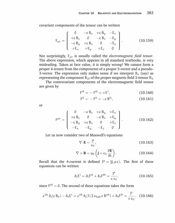
“chapter10” — 2007/12/14 — 13:59 — page 383 — #33
CHAPTER 10 RELATIVITY AND ELECTROMAGNETISM 383
covariant components of the tensor can be written
Fµν =
0 −cBz +cBy −Ex
+cBz 0 −cBx −Ey
−cBy +cBx 0 −Ez
+Ex +Ey +Ez 0
. (10.159)
Not surprisingly, Fµν is usually called the electromagnetic field tensor.The above expression, which appears in all standard textbooks, is verymisleading. Taken at face value, it is simply wrong! We cannot form aproper 4-tensor from the components of a proper 3-vector and a pseudo-3-vector. The expression only makes sense if we interpret Bx (say) asrepresenting the component B23 of the proper magnetic field 3-tensor Bij
The contravariant components of the electromagnetic field tensorare given by
Fi4 = − F4i = +Ei, (10.160)
Fij = − Fji = −cBij, (10.161)
or
Fµν =
0 −cBz +cBy +Ex
+cBz 0 −cBx +Ey
−cBy +cBx 0 +Ez
−Ex −Ey −Ez 0
. (10.162)
Let us now consider two of Maxwell’s equations:
∇·E =ρ
ε0, (10.163)
∇ × B = µ0
(j + ε0
∂E∂t
). (10.164)
Recall that the 4-current is defined Jµ = (j, ρ c). The first of theseequations can be written
∂iEi = ∂iF
i4 + ∂4F44 =
J4
c ε0. (10.165)
since F44 = 0. The second of these equations takes the form
εijk ∂j(cBk) − ∂4Ei = εijk ∂j(1/2 εkab cB
ab) + ∂4F4i =
Ji
c ε0. (10.166)
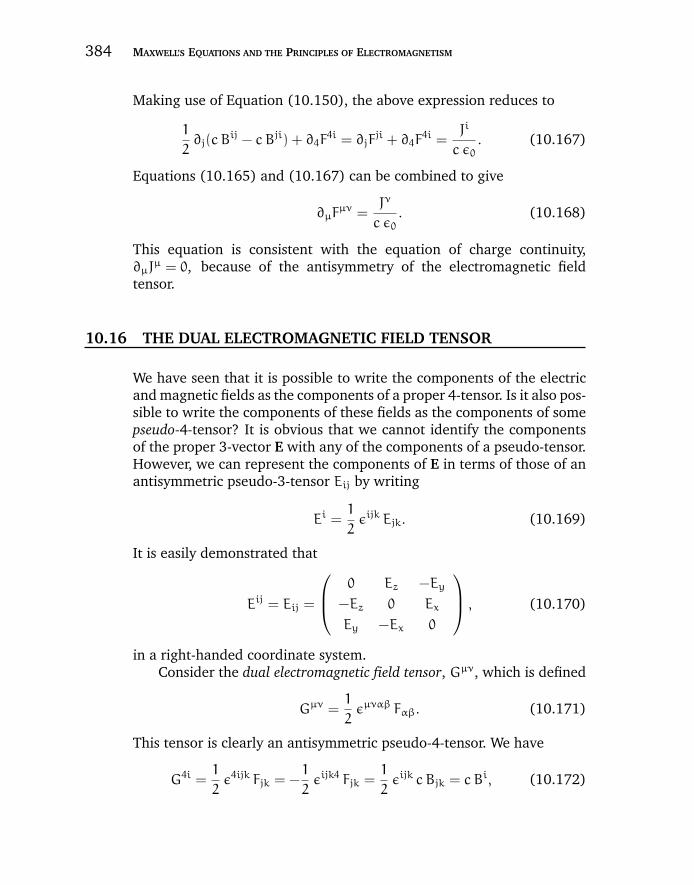
“chapter10” — 2007/12/14 — 13:59 — page 384 — #34
384 MAXWELL’S EQUATIONS AND THE PRINCIPLES OF ELECTROMAGNETISM
Making use of Equation (10.150), the above expression reduces to
1
2∂j(cB
ij − cBji) + ∂4F4i = ∂jF
ji + ∂4F4i =
Ji
c ε0. (10.167)
Equations (10.165) and (10.167) can be combined to give
∂µFµν =
Jν
c ε0. (10.168)
This equation is consistent with the equation of charge continuity,∂µJ
µ = 0, because of the antisymmetry of the electromagnetic fieldtensor.
10.16 THE DUAL ELECTROMAGNETIC FIELD TENSOR
We have seen that it is possible to write the components of the electricand magnetic fields as the components of a proper 4-tensor. Is it also pos-sible to write the components of these fields as the components of somepseudo-4-tensor? It is obvious that we cannot identify the componentsof the proper 3-vector E with any of the components of a pseudo-tensor.However, we can represent the components of E in terms of those of anantisymmetric pseudo-3-tensor Eij by writing
Ei =1
2εijk Ejk. (10.169)
It is easily demonstrated that
Eij = Eij =
0 Ez −Ey
−Ez 0 Ex
Ey −Ex 0
, (10.170)
in a right-handed coordinate system.Consider the dual electromagnetic field tensor, Gµν, which is defined
Gµν =1
2εµναβ Fαβ. (10.171)
This tensor is clearly an antisymmetric pseudo-4-tensor. We have
G4i =1
2ε4ijk Fjk = −
1
2εijk4 Fjk =
1
2εijk c Bjk = cBi, (10.172)
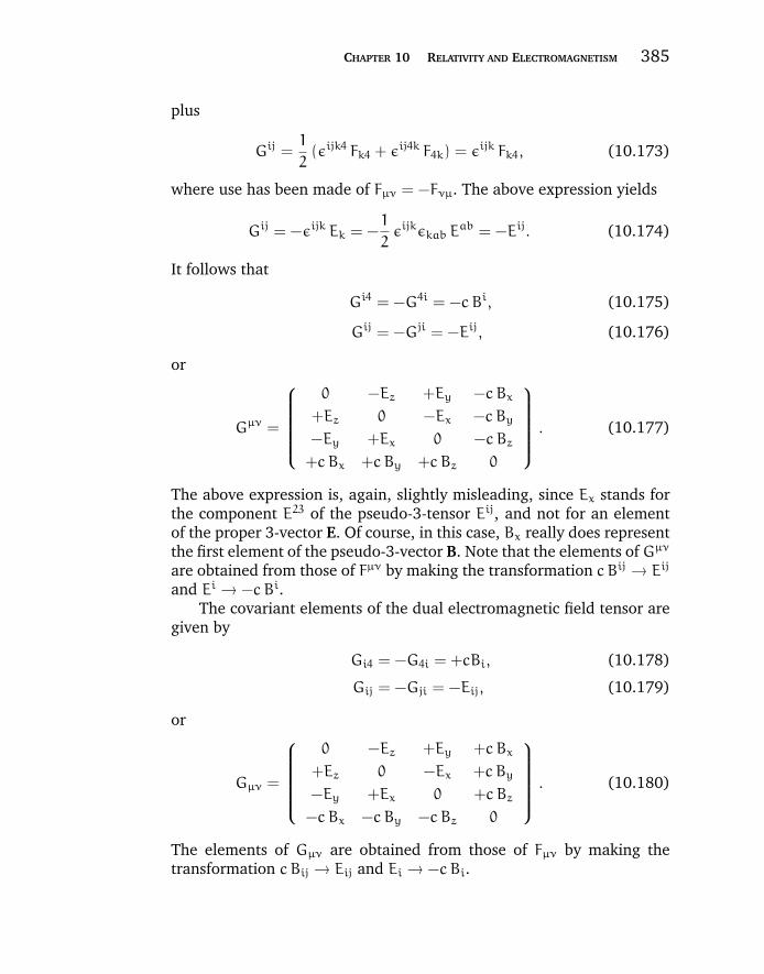
“chapter10” — 2007/12/14 — 13:59 — page 385 — #35
CHAPTER 10 RELATIVITY AND ELECTROMAGNETISM 385
plus
Gij =1
2(εijk4 Fk4 + εij4k F4k) = εijk Fk4, (10.173)
where use has been made of Fµν = −Fνµ. The above expression yields
Gij = −εijk Ek = −1
2εijkεkab E
ab = −Eij. (10.174)
It follows that
Gi4 = −G4i = −cBi, (10.175)
Gij = −Gji = −Eij, (10.176)
or
Gµν =
0 −Ez +Ey −cBx
+Ez 0 −Ex −cBy
−Ey +Ex 0 −cBz
+cBx +cBy +cBz 0
. (10.177)
The above expression is, again, slightly misleading, since Ex stands forthe component E23 of the pseudo-3-tensor Eij, and not for an elementof the proper 3-vector E. Of course, in this case, Bx really does representthe first element of the pseudo-3-vector B. Note that the elements ofGµν
are obtained from those of Fµν by making the transformation cBij → Eij
and Ei → −cBi.The covariant elements of the dual electromagnetic field tensor are
given by
Gi4 = −G4i = +cBi, (10.178)
Gij = −Gji = −Eij, (10.179)
or
Gµν =
0 −Ez +Ey +cBx
+Ez 0 −Ex +cBy
−Ey +Ex 0 +cBz
−cBx −cBy −cBz 0
. (10.180)
The elements of Gµν are obtained from those of Fµν by making thetransformation cBij → Eij and Ei → −cBi.
“chapter10” — 2007/12/14 — 13:59 — page 386 — #36
386 MAXWELL’S EQUATIONS AND THE PRINCIPLES OF ELECTROMAGNETISM
Let us now consider the two Maxwell equations
∇·B = 0, (10.181)
∇ × E = −∂B∂t. (10.182)
The first of these equations can be written
−∂i (cBi) = ∂iG
i4 + ∂4G44 = 0, (10.183)
since G44 = 0. The second equation takes the form
εijk∂jEk = εijk∂j(1/2 εkabEab) = ∂jE
ij = −∂4 (cBi), (10.184)
or
∂jGji + ∂4G
4i = 0. (10.185)
Equations (10.183) and (10.185) can be combined to give
∂µGµν = 0. (10.186)
Thus, we conclude that Maxwell’s equations for the electromagneticfields are equivalent to the following pair of 4-tensor equations:
∂µFµν =
Jν
c ε0, (10.187)
∂µGµν = 0. (10.188)
It is obvious from the form of these equations that the laws ofelectromagnetism are invariant under translations, rotations, specialLorentz transformations, parity inversions, or any combination of thesetransformations.
10.17 TRANSFORMATION OF FIELDS
The electromagnetic field tensor transforms according to the standardrule
Fµ′ν ′
= Fµν pµ′µ p
ν ′ν . (10.189)
“chapter10” — 2007/12/14 — 13:59 — page 387 — #37
CHAPTER 10 RELATIVITY AND ELECTROMAGNETISM 387
This easily yields the celebrated rules for transforming electromagneticfields:
E ′‖ = E‖, (10.190)
B ′‖ = B‖, (10.191)
E ′⊥ = γ (E⊥ + v × B), (10.192)
B ′⊥ = γ (B⊥ − v × E/c2), (10.193)
where v is the relative velocity between the primed and unprimedframes, and the perpendicular and parallel directions are, respectively,perpendicular and parallel to v.
At this stage, we may conveniently note two important invariants ofthe electromagnetic field. They are
1
2Fµν F
µν = c2 B2 − E2, (10.194)
and1
4Gµν F
µν = cE·B. (10.195)
The first of these quantities is a proper-scalar, and the second a pseudo-scalar.
10.18 POTENTIAL DUE TO A MOVING CHARGE
Suppose that a particle carrying a charge e moves with uniform velocityu through a frame S. Let us evaluate the vector potential, A, and thescalar potential, φ, due to this charge at a given event P in S.
Let us choose coordinates in S so that P = (0, 0, 0, 0) and u = (u, 0, 0).Let S ′ be that frame in the standard configuration with respect to S inwhich the charge is (permanently) at rest at (say) the point (x ′, y ′, z ′).In S ′, the potential at P is the usual potential due to a stationary charge,
A ′ = 0, (10.196)
φ ′ =e
4πε0 r ′ , (10.197)
where r ′ =√x
′2 + y′2 + z
′2. Let us now transform these equationsdirectly into the frame S. Since Aµ = (cA, φ) is a contravariant 4-vector, its components transform according to the standard rules
“chapter10” — 2007/12/14 — 13:59 — page 388 — #38
388 MAXWELL’S EQUATIONS AND THE PRINCIPLES OF ELECTROMAGNETISM
(10.75)–(10.78). Thus,
cA1 = γ(cA ′
1 +u
cφ ′)
=γue
4πε0 c r ′ , (10.198)
cA2 = cA ′2 = 0, (10.199)
cA3 = cA ′3 = 0, (10.200)
φ = γ(φ ′ +
u
ccA ′
1
)=
γ e
4πε0 r ′ , (10.201)
since β = −u/c in this case. It remains to express the quantity r ′ interms of quantities measured in S. The most physically meaningful wayof doing this is to express r ′ in terms of retarded values in S. Considerthe retarded event at the charge for which, by definition, r ′ = −c t ′ andr = −c t. Using the standard Lorentz transformation, (10.24)–(10.27),we find that
r ′ = −c t ′ = −c γ (t− ux/c2) = r γ (1+ ur/c), (10.202)
where ur = ux/r = r ·u/r denotes the radial velocity of the change in S.We can now rewrite Equations (10.198)–(10.201) in the form
A =µ0 e
4π
[u]
[r+ r ·u/c] , (10.203)
φ =e
4πε0
1
[r+ r ·u/c] , (10.204)
where the square brackets, as usual, indicate that the enclosed quantitiesmust be retarded. For a uniformly moving charge, the retardation of uis, of course, superfluous. However, since
Φµ =1
4πε0 c
∫[Jµ]
rdV, (10.205)
it is clear that the potentials depend only on the (retarded) velocityof the charge, and not on its acceleration. Consequently, the expres-sions (10.203) and (10.204) give the correct potentials for an arbitrarilymoving charge. They are known as the Lienard-Wiechert potentials.
10.19 FIELD DUE TO A MOVING CHARGE
Although the fields generated by a uniformly moving charge can be cal-culated from the expressions (10.203) and (10.204) for the potentials,it is simpler to calculate them from first principles.
“chapter10” — 2007/12/14 — 13:59 — page 389 — #39
CHAPTER 10 RELATIVITY AND ELECTROMAGNETISM 389
Let a charge e, whose position vector at time t = 0 is r, move withuniform velocity u in a frame S whose x-axis has been chosen in thedirection of u. We require to find the field strengths E and B at the eventP = (0, 0, 0, 0). Let S ′ be that frame in standard configuration with S inwhich the charge is permanently at rest. In S ′, the field is given by
B ′ = 0, (10.206)
E ′ = −e
4πε0
r ′
r ′ 3 . (10.207)
This field must now be transformed into the frame S. The direct method,using Equations (10.190)–(10.193), is somewhat simpler here, but weshall use a somewhat indirect method because of its intrinsic interest.
In order to express Equations (10.206) and (10.207) in tensor form,we need the electromagnetic field tensor Fµν on the left-hand side, andthe position 4-vector Rµ = (r, c t) and the scalar e/(4πε0 r ′3) on the right-hand side. (We regard r ′ as an invariant for all observers.) To get avanishing magnetic field in S ′, we multiply on the right by the 4-velocityUµ = γ(u) (u, c), thus tentatively arriving at the equation
Fµν =e
4πε0 c r ′ 3 Uµ Rν. (10.208)
Recall that F4i = −Ei and Fij = −cBij. However, this equation cannot becorrect, because the antisymmetric tensor Fµν can only be equated toanother antisymmetric tensor. Consequently, let us try
Fµν =e
4πε0 c r ′ 3 (Uµ Rν −Uν Rµ). (10.209)
This is found to give the correct field at P in S ′, as long as Rµ refers to anyevent whatsoever at the charge. It only remains to interpret (10.209) inS. It is convenient to choose for Rµ that event at the charge at whicht = 0 (not the retarded event). Thus,
Fjk = −cBjk =e
4πε0 c r ′ 3 γ(u) (uj rk − uk rj), (10.210)
giving
Bi =1
2εijkB
jk = −µ0 e
4π r ′ 3 γ(u) εijk uj rk, (10.211)
or
B = −µ0 e γ
4π r ′ 3 u × r. (10.212)
“chapter10” — 2007/12/14 — 13:59 — page 390 — #40
390 MAXWELL’S EQUATIONS AND THE PRINCIPLES OF ELECTROMAGNETISM
Likewise,
F4i = −Ei =e γ
4πε0 r ′ 3 ri, (10.213)
or
E = −e γ
4πε0 r ′ 3 r. (10.214)
Lastly, we must find an expression for r ′ 3 in terms of quantities measuredin S at time t = 0. If t ′ is the corresponding time in S ′ at the charge, wehave
r ′ 2 = r2 + c2 t ′ 2 = r2 +γ2 u2 x2
c2= r2
(1+
γ2 u 2r
c2
). (10.215)
Thus,
E = −e
4πε0
γ
r3 (1+ u 2r γ
2/c2)3/2r, (10.216)
B = −µ0 e
4π
γ
r3 (1+ u 2r γ
2/c2)3/2u × r =
1
c2u × E. (10.217)
Note that E acts in line with the point which the charge occupies atthe instant of measurement, despite the fact that, owing to the finitespeed of propagation of all physical effects, the behavior of the chargeduring a finite period before that instant can no longer affect the mea-surement. Note also that, unlike Equations (10.203) and (10.204), theabove expressions for the fields are not valid for an arbitrarily movingcharge, nor can they be made valid by merely using retarded values.For whereas acceleration does not affect the potentials, it does affect thefields, which involve the derivatives of the potential.
For low velocities, u/c → 0, Equations (10.216) and (10.217) reduceto the well-known Coulomb and Biot-Savart fields. However, at highvelocities, γ(u) 1, the fields exhibit some interesting behavior. Thepeak electric field, which occurs at the point of closest approach ofthe charge to the observation point, becomes equal to γ times its non-relativistic value. However, the duration of appreciable field strength atthe point P is decreased. A measure of the time interval over which thefield is appreciable is
∆t ∼b
γ c, (10.218)
“chapter10” — 2007/12/14 — 13:59 — page 391 — #41
CHAPTER 10 RELATIVITY AND ELECTROMAGNETISM 391
where b is the distance of closest approach (assuming γ 1). As γincreases, the peak field increases in proportion, but its duration goes inthe inverse proportion. The time integral of the field is independent of γ.As γ → ∞, the observer at P sees electric and magnetic fields which areindistinguishable from the fields of a pulse of plane polarized radiationpropagating in the x-direction. The direction of polarization is along theradius vector pointing toward the particle’s actual position at the timeof observation.
10.20 RELATIVISTIC PARTICLE DYNAMICS
Consider a particle which, in its instantaneous rest frame S0, has massm0 and constant acceleration in the x-direction a0. Let us transform toa frame S, in the standard configuration with respect to S0, in which theparticle’s instantaneous velocity is u. What is the value of a, the particle’sinstantaneous x-acceleration, in S?
The easiest way in which to answer this question is to consider theacceleration 4-vector [see Equation (10.107)]
Aµ = γ
(dγ
dtu + γ a, c
dγ
dt
). (10.219)
Using the standard transformation, (10.75)–(10.78), for 4-vectors, weobtain
a0 = γ3 a, (10.220)dγ
dt=ua0
c2. (10.221)
Equation (10.220) can be written
f = m0 γ3 du
dt, (10.222)
where f = m0 a0 is the constant force (in the x-direction) acting on theparticle in S0.
Equation (10.222) is equivalent to
f =d(mu)
dt, (10.223)
where
m = γm0. (10.224)
“chapter10” — 2007/12/14 — 13:59 — page 392 — #42
392 MAXWELL’S EQUATIONS AND THE PRINCIPLES OF ELECTROMAGNETISM
Thus, we can account for the ever-decreasing acceleration of a particlesubject to a constant force [see Equation (10.220)] by supposing thatthe inertial mass of the particle increases with its velocity according tothe rule (10.224). Henceforth, m0 is termed the rest mass, and m theinertial mass.
The rate of increase of the particle’s energy E satisfies
dE
dt= f u = m0 γ
3 udu
dt. (10.225)
This equation can be written
dE
dt=d(mc2)
dt, (10.226)
which can be integrated to yield Einstein’s famous formula
E = mc2. (10.227)
The 3-momentum of a particle is defined
p = mu, (10.228)
where u is its 3-velocity. Thus, by analogy with Equation (10.223),Newton’s law of motion can be written
f =dpdt, (10.229)
where f is the 3-force acting on the particle.The 4-momentum of a particle is defined
Pµ = m0Uµ = γm0 (u, c) = (p, E/c), (10.230)
where Uµ is its 4-velocity. The 4-force acting on the particle obeys
Fµ =dPµ
dτ= m0 A
µ, (10.231)
where Aµ is its 4-acceleration. It is easily demonstrated that
Fµ = γ
(f , c
dm
dt
)= γ
(f ,
f ·uc
), (10.232)
since
dE
dt= f ·u. (10.233)
“chapter10” — 2007/12/14 — 13:59 — page 393 — #43
CHAPTER 10 RELATIVITY AND ELECTROMAGNETISM 393
10.21 FORCE ON A MOVING CHARGE
The electromagnetic 3-force acting on a charge emoving with 3-velocityu is given by the well-known formula
f = e (E + u × B). (10.234)
When written in component form this expression becomes
fi = e (Ei + εijk uj Bk), (10.235)
or
fi = e (Ei + Bij uj), (10.236)
where use has been made of Equation (10.147).Recall that the components of the E and B fields can be written in
terms of an antisymmetric electromagnetic field tensor Fµν via
Fi4 = − F4i = −Ei, (10.237)
Fij = − Fji = −cBij. (10.238)
Equation (10.236) can be written
fi = −e
γ c(Fi4 U
4 + Fij Uj), (10.239)
where Uµ = γ (u, c) is the particle’s 4-velocity. It is easily demonstratedthat
f ·uc
=e
cE·u =
e
cEi u
i =e
γ c(F4i U
i + F44 U4). (10.240)
Thus, the 4-force acting on the particle,
Fµ = γ
(−f ,
f ·uc
), (10.241)
can be written in the form
Fµ =e
cFµν U
ν. (10.242)
The skew symmetry of the electromagnetic field tensor ensures that
Fµ Uµ =e
cFµν U
µ Uν = 0. (10.243)
This is an important result, since it ensures that electromagnetic fieldsdo not change the rest mass of charged particles. In order to appreciate
“chapter10” — 2007/12/14 — 13:59 — page 394 — #44
394 MAXWELL’S EQUATIONS AND THE PRINCIPLES OF ELECTROMAGNETISM
this, let us assume that the rest mass m0 is not a constant. Since
Fµ =d(m0Uµ)
dτ= m0 Aµ +
dm0
dτUµ, (10.244)
we can use the standard results Uµ Uµ = c2 and Aµ Uµ = 0 to give
Fµ Uµ = c2dm0
dτ. (10.245)
Thus, if rest mass is to remain an invariant, it is imperative that all lawsof Physics predict 4-forces acting on particles which are orthogonal tothe particles’ 4-velocities. The laws of electromagnetism pass this test.
10.22 THE ELECTROMAGNETIC ENERGY TENSOR
Consider a continuous volume distribution of charged matter in the pres-ence of an electromagnetic field. Let there be n0 particles per unit propervolume (unit volume determined in the local rest frame), each carryinga charge e. Consider an inertial frame in which the 3-velocity field ofthe particles is u. The number density of the particles in this frame isn = γ(u)n0. The charge density and the 3-current due to the particlesare ρ = en and j = enu, respectively. Multiplying Equation (10.242) bythe proper number density of particles, n0, we obtain an expression
fµ = c−1 Fµν Jν (10.246)
for the 4-force fµ acting on unit proper volume of the distribution due tothe ambient electromagnetic fields. Here, we have made use of the def-inition Jµ = en0 U
µ. It is easily demonstrated, using some of the resultsobtained in the previous section, that
fµ =
(ρE + j × B,
E·jc
). (10.247)
The above expression remains valid when there are many charge species(e.g., electrons and ions) possessing different number density and 3-velocity fields. The 4-vector fµ is usually called the Lorentz force density.
We know that Maxwell’s equations reduce to
∂µFµν =
Jν
c ε0, (10.248)
∂µGµν = 0, (10.249)
“chapter10” — 2007/12/14 — 13:59 — page 395 — #45
CHAPTER 10 RELATIVITY AND ELECTROMAGNETISM 395
where Fµν is the electromagnetic field tensor, and Gµν is its dual. As iseasily verified, Equation (10.249) can also be written in the form
∂µFνσ + ∂νFσµ + ∂σFµν = 0. (10.250)
Equations (10.246) and (10.248) can be combined to give
fν = ε0 Fνσ ∂µFµσ. (10.251)
This expression can also be written
fν = ε0 [∂µ(Fµσ Fνσ) − Fµσ ∂µFνσ] . (10.252)
Now,
Fµσ ∂µFνσ =1
2Fµσ(∂µFνσ + ∂σFµν), (10.253)
where use has been made of the antisymmetry of the electromagneticfield tensor. It follows from Equation (10.250) that
Fµσ ∂µFνσ = −1
2Fµσ ∂νFσµ =
1
4∂ν(F
µσ Fµσ). (10.254)
Thus,
fν = ε0
[∂µ(F
µσ Fνσ) −1
4∂ν(F
µσ Fµσ)
]. (10.255)
The above expression can also be written
fν = −∂µTµν, (10.256)
where
Tµν = ε0
[Fµσ Fσν +
1
4δµν (Fρσ Fρσ)
](10.257)
is called the electromagnetic energy tensor. Note that Tµν is a proper4-tensor. It follows from Equations (10.159), (10.162), and (10.194)that
Tij = ε0 Ei Ej +
Bi Bj
µ0− δij
1
2
(ε0 E
k Ek +Bk Bk
µ0
), (10.258)
“chapter10” — 2007/12/14 — 13:59 — page 396 — #46
396 MAXWELL’S EQUATIONS AND THE PRINCIPLES OF ELECTROMAGNETISM
Ti4 = −T4i =εijk Ej Bk
µ0 c, (10.259)
T44 =1
2
(ε0 E
k Ek +Bk Bk
µ0
). (10.260)
Equation (10.256) can also be written
fν = −∂µTµν, (10.261)
where Tµν is a symmetric tensor whose elements are
Tij = − ε0 Ei Ej −
Bi Bj
µ0+ δij
1
2
(ε0 E
2 +B2
µ0
), (10.262)
Ti4 = T4i =(E × B)i
µ0 c, (10.263)
T44 =1
2
(ε0 E
2 +B2
µ0
). (10.264)
Consider the time-like component of Equation (10.261). It followsfrom Equation (10.247) that
E·jc
= −∂iTi4 − ∂4T
44. (10.265)
This equation can be rearranged to give
∂U
∂t+ ∇·u = −E·j, (10.266)
where U = T44 and ui = cTi4, so that
U =ε0 E
2
2+B2
2µ0, (10.267)
and
u =E × Bµ0
. (10.268)
The right-hand side of Equation (10.266) represents the rate per unitvolume at which energy is transferred from the electromagnetic fieldto charged particles. It is clear, therefore, that Equation (10.266) isan energy conservation equation for the electromagnetic field (see Sec-tion 8.2). The proper 3-scalar U can be identified as the energy density
“chapter10” — 2007/12/14 — 13:59 — page 397 — #47
CHAPTER 10 RELATIVITY AND ELECTROMAGNETISM 397
of the electromagnetic field, whereas the proper 3-vector u is the energyflux due to the electromagnetic field: i.e., the Poynting flux.
Consider the space-like components of Equation (10.261). It is easilydemonstrated that these reduce to
∂g∂t
+ ∇ ·G = −ρE − j × B, (10.269)
where Gij = Tij and gi = T4i/c, or
Gij = −ε0 Ei Ej −
Bi Bj
µ0+ δij
1
2
(ε0 E
2 +B2
µ0
), (10.270)
and
g =uc2
= ε0 E × B. (10.271)
Equation (10.269) is basically a momentum conservation equation forthe electromagnetic field (see Section 8.4). The right-hand side repre-sents the rate per unit volume at which momentum is transferred fromthe electromagnetic field to charged particles. The symmetric proper 3-tensorGij specifies the flux of electromagnetic momentum parallel to theith axis crossing a surface normal to the jth axis. The proper 3-vector grepresents the momentum density of the electromagnetic field. It is clearthat the energy conservation law (10.266) and the momentum conser-vation law (10.269) can be combined together to give the relativisticallyinvariant energy-momentum conservation law (10.261).
10.23 ACCELERATED CHARGES
Let us calculate the electric and magnetic fields observed at position xi
and time t due to a charge ewhose retarded position and time are xi ′ andt ′, respectively. From now on (xi, t) is termed the field point and (xi
′, t ′)
is termed the source point. It is assumed that we are given the retardedposition of the charge as a function of its retarded time: i.e., xi ′(t ′). Theretarded velocity and acceleration of the charge are
ui =dxi
′
dt ′ , (10.272)
and
.ui=dui
dt ′ , (10.273)
“chapter10” — 2007/12/14 — 13:59 — page 398 — #48
398 MAXWELL’S EQUATIONS AND THE PRINCIPLES OF ELECTROMAGNETISM
respectively. The radius vector r is defined to extend from the retardedposition of the charge to the field point, so that ri = xi − xi
′. (Note thatthis is the opposite convention to that adopted in Sections 10.18 and10.19). It follows that
drdt ′ = −u. (10.274)
The field and the source point variables are connected by the retardationcondition
r(xi, xi′) =
[(xi − xi
′) (xi − xi
′)]1/2
= c (t− t ′). (10.275)
The potentials generated by the charge are given by the Lienard-Wiechert formulae,
A(xi, t) =µ0 e
4π
us, (10.276)
φ(xi, t) =e
4πε0
1
s, (10.277)
where s = r− r ·u/c is a function both of the field point and the sourcepoint variables. Recall that the Lienard-Wiechert potentials are valid foraccelerating, as well as uniformly moving, charges.
The fields E and B are derived from the potentials in the usualmanner:
E = −∇φ−∂A∂t, (10.278)
B = ∇ × A. (10.279)
However, the components of the gradient operator ∇ are partial deriva-tives at constant time, t, and not at constant time, t ′. Partial differentia-tion with respect to the xi compares the potentials at neighboring pointsat the same time, but these potential signals originate from the charge atdifferent retarded times. Similarly, the partial derivative with respect tot implies constant xi, and, hence, refers to the comparison of the poten-tials at a given field point over an interval of time during which theretarded coordinates of the source have changed. Since we only knowthe time variation of the particle’s retarded position with respect to t ′we must transform ∂/∂t|xi and ∂/∂xi|t to expressions involving ∂/∂t ′|xi
and ∂/∂xi|t ′ .
“chapter10” — 2007/12/14 — 13:59 — page 399 — #49
CHAPTER 10 RELATIVITY AND ELECTROMAGNETISM 399
Now, since xi ′ is assumed to be given as a function of t ′, we have
r(xi, xi′(t ′) ) ≡ r(xi, t ′) = c (t− t ′), (10.280)
which is a functional relationship between xi, t, and t ′. Note that(∂r
∂t ′
)xi
= −r ·ur. (10.281)
It follows that
∂r
∂t= c
(1−
∂t ′
∂t
)=∂r
∂t ′∂t ′
∂t= −
r ·ur
∂t ′
∂t, (10.282)
where all differentiation is at constant xi. Thus,
∂t ′
∂t=
1
1− r ·u/r c =r
s, (10.283)
giving
∂
∂t=r
s
∂
∂t ′ . (10.284)
Similarly,
∇r = −c∇t ′ = ∇ ′r+∂r
∂t ′ ∇t ′ =rr
−r ·ur
∇t ′, (10.285)
where ∇ ′ denotes differentiation with respect to xi at constant t ′. Itfollows that
∇t ′ = −rs c, (10.286)
so that
∇ = ∇ ′ −rs c
∂
∂t ′ . (10.287)
Equation (10.278) yields
4πε0
eE =
∇ss2
−∂
∂t
us c2
, (10.288)
or
4πε0
eE =
∇ ′ss2
−rs3 c
∂s
∂t ′ −r
s2 c2.u +
rus3 c2
∂s
∂t ′ . (10.289)

“chapter10” — 2007/12/14 — 13:59 — page 400 — #50
400 MAXWELL’S EQUATIONS AND THE PRINCIPLES OF ELECTROMAGNETISM
However,
∇ ′s =rr
−uc, (10.290)
and
∂s
∂t ′ =∂r
∂t ′ −r· .uc
+u·uc
= −r·ur
−r· .uc
+u2
c. (10.291)
Thus,
4πε0
eE =
1
s2 r
(r −
ruc
)+
1
s3 c
(r −
ruc
)(r ·ur
−u2
c+
r· .uc
)−
r
s2 c2.u,
(10.292)
which reduces to
4πε0
eE =
1
s3
(r −
ruc
)(1−
u2
c2
)+
1
s3 c2
(r ×
[(r −
ruc
)× .
u]).
(10.293)
Similarly,
4π
µ0 eB = ∇ × u
s= −
∇ ′s× us2
−rs c
×( .
us
−us2∂s
∂t ′
), (10.294)
or
4π
µ0 eB = −
r × us2 r
−rs c
×[ .
us
+us2
(r ·ur
+r· .uc
−u2
c
)], (10.295)
which reduces to
4π
µ0 eB =
u × rs3
(1−
u2
c2
)+
1
s3 c
rr
×(
r ×[(
r −ruc
)× .
u]).
(10.296)
A comparison of Equations (10.293) and (10.296) yields
B =r × Er c
. (10.297)
Thus, the magnetic field is always perpendicular to E and the retardedradius vector r. Note that all terms appearing in the above formulae areretarded.
“chapter10” — 2007/12/14 — 13:59 — page 401 — #51
CHAPTER 10 RELATIVITY AND ELECTROMAGNETISM 401
The electric field is composed of two separate parts. The first term inEquation (10.293) varies as 1/r2 for large distances from the charge. Wecan think of ru = r − ru/c as the virtual present radius vector: i.e., theradius vector directed from the position the charge would occupy at timet if it had continued with uniform velocity from its retarded position tothe field point. In terms of ru, the 1/r2 field is simply
Einduction =e
4πε0
1− u2/c2
s3ru. (10.298)
We can rewrite the expression (10.216) for the electric field generatedby a uniformly moving charge in the form
E =e
4πε0
1− u2/c2
r 30 (1− u2/c2 + u 2r /c
2)3/2r0, (10.299)
where r0 is the radius vector directed from the present position of thecharge at time t to the field point, and ur = u · r0/r0. For the case ofuniform motion, the relationship between the retarded radius vector rand the actual radius vector r0 is simply
r0 = r −r
cu. (10.300)
It is straightforward to demonstrate that
s = r0
√1− u2/c2 + u 2
r /c2 (10.301)
in this case. Thus, the electric field generated by a uniformly movingcharge can be written
E =e
4πε0
1− u2/c2
s3r0. (10.302)
Since ru = r0 for the case of a uniformly moving charge, it is clear thatEquation (10.298) is equivalent to the electric field generated by a uni-formly moving charge located at the position the charge would occupyif it had continued with uniform velocity from its retarded position.
The second term in Equation (10.293),
Eradiation =e
4πε0 c2r × (ru× .
u)
s3, (10.303)
is of order 1/r, and, therefore, represents a radiation field. Similarconsiderations hold for the two terms of Equation (10.296).
“chapter10” — 2007/12/14 — 13:59 — page 402 — #52
402 MAXWELL’S EQUATIONS AND THE PRINCIPLES OF ELECTROMAGNETISM
10.24 THE LARMOR FORMULA
Let us transform to the inertial frame in which the charge is instanta-neously at rest at the origin at time t = 0. In this frame, u c, so thatru r and s r for events which are sufficiently close to the origin att = 0 that the retarded charge still appears to travel with a velocity whichis small compared to that of light. It follows from the previous sectionthat
Erad e
4πε0 c2r × (r× .
u)
r3, (10.304)
Brad e
4πε0 c3
.u ×rr2
. (10.305)
Let us define spherical polar coordinates whose axis points alongthe direction of instantaneous acceleration of the charge. It is easilydemonstrated that
Eθ e
4πε0 c2sin θr
.u, (10.306)
Bφ e
4πε0 c3sin θr
.u . (10.307)
These fields are identical to those of a radiating dipole whose axisis aligned along the direction of instantaneous acceleration (see Sec-tion 9.2). The radial Poynting flux is given by
Eθ Bφ
µ0=
e2
16π2ε0 c3sin2 θr2
.u2. (10.308)
We can integrate this expression to obtain the instantaneous powerradiated by the charge
P =e2
6πε0 c3.u2. (10.309)
This is known as Larmor’s formula. Note that zero net momentum iscarried off by the fields (10.306) and (10.307).
In order to proceed further, it is necessary to prove two usefultheorems. The first theorem states that if a 4-vector field Tµ satisfies
∂µTµ = 0, (10.310)
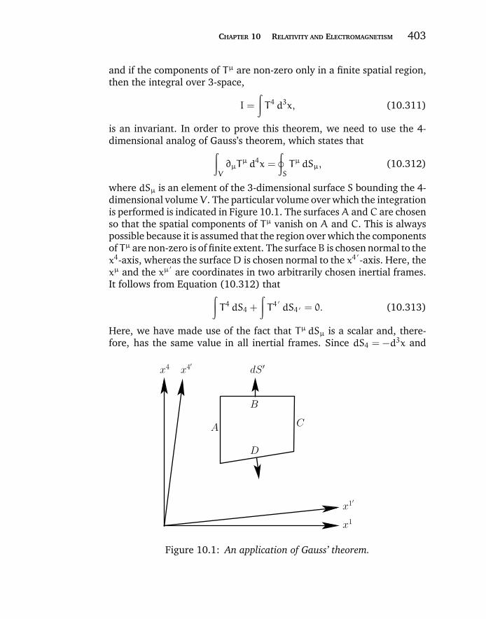
“chapter10” — 2007/12/14 — 13:59 — page 403 — #53
CHAPTER 10 RELATIVITY AND ELECTROMAGNETISM 403
and if the components of Tµ are non-zero only in a finite spatial region,then the integral over 3-space,
I =
∫T4 d3x, (10.311)
is an invariant. In order to prove this theorem, we need to use the 4-dimensional analog of Gauss’s theorem, which states that∫
V
∂µTµ d4x =
∮S
Tµ dSµ, (10.312)
where dSµ is an element of the 3-dimensional surface S bounding the 4-dimensional volumeV. The particular volume over which the integrationis performed is indicated in Figure 10.1. The surfacesA andC are chosenso that the spatial components of Tµ vanish on A and C. This is alwayspossible because it is assumed that the region over which the componentsof Tµ are non-zero is of finite extent. The surfaceB is chosen normal to thex4-axis, whereas the surfaceD is chosen normal to the x4
′-axis. Here, the
xµ and the xµ′
are coordinates in two arbitrarily chosen inertial frames.It follows from Equation (10.312) that∫
T4 dS4 +
∫T4
′dS4 ′ = 0. (10.313)
Here, we have made use of the fact that Tµ dSµ is a scalar and, there-fore, has the same value in all inertial frames. Since dS4 = −d3x and
A
x1′
C
D
B
dS ′x4 x4′
x1
Figure 10.1: An application of Gauss’ theorem.
“chapter10” — 2007/12/14 — 13:59 — page 404 — #54
404 MAXWELL’S EQUATIONS AND THE PRINCIPLES OF ELECTROMAGNETISM
dS4 ′ = d3x ′ it follows that I =∫T4 d3x is an invariant under a Lorentz
transformation. Incidentally, the above argument also demonstrates thatI is constant in time (just take the limit in which the two inertial framesare identical).
The second theorem is an extension of the first. Suppose that a 4-tensor field Qµν satisfies
∂µQµν = 0, (10.314)
and has components which are only non-zero in a finite spatial region.LetAµ be a 4-vector whose coefficients do not vary with position in space-time. It follows that Tµ = AνQ
µν satisfies Equation (10.310). Therefore,
I =
∫AνQ
4ν d3x (10.315)
is an invariant. However, we can write
I = Aµ Bµ, (10.316)
where
Bµ =
∫Q4µ d3x. (10.317)
It follows from the quotient rule that ifAµ Bµ is an invariant for arbitraryAµ then Bµ must transform as a constant (in time) 4-vector.
These two theorems enable us to convert differential conservationlaws into integral conservation laws. For instance, in differential form,the conservation of electrical charge is written
∂µJµ = 0. (10.318)
However, from Equation (10.313) this immediately implies that
Q =1
c
∫J4 d3x =
∫ρd3x (10.319)
is an invariant. In other words, the total electrical charge contained inspace is both constant in time, and the same in all inertial frames.
Suppose that S is the instantaneous rest frame of the charge. Letus consider the electromagnetic energy tensor Tµν associated with allof the radiation emitted by the charge between times t = 0 and t = dt.According to Equation (10.261), this tensor field satisfies
∂µTµν = 0, (10.320)
“chapter10” — 2007/12/14 — 13:59 — page 405 — #55
CHAPTER 10 RELATIVITY AND ELECTROMAGNETISM 405
apart from a region of space of measure zero in the vicinity of the charge.Furthermore, the region of space over which Tµν is non-zero is clearlyfinite, since we are only considering the fields emitted by the charge in asmall time interval, and these fields propagate at a finite velocity. Thus,according to the second theorem,
Pµ =1
c
∫T4µ d3x (10.321)
is a 4-vector. It follows from Section 10.22 that we can write Pµ =(dp, dE/c), where dp and dE are the total momentum and energy carriedoff by the radiation emitted between times t = 0 and t = dt, respectively.As we have already mentioned, dp = 0 in the instantaneous rest frame S.Transforming to an arbitrary inertial frame S ′, in which the instantaneousvelocity of the charge is u, we obtain
dE′= γ(u)
(dE+ udp1
)= γdE. (10.322)
However, the time interval over which the radiation is emitted in S ′ isdt ′ = γdt. Thus, the instantaneous power radiated by the charge,
P ′ =dE ′
dt ′ =dE
dt= P, (10.323)
is the same in all inertial frames.We can make use of the fact that the power radiated by an acceler-
ating charge is Lorentz invariant to find a relativistic generalization ofthe Larmor formula, (10.309), which is valid in all inertial frames. Weexpect the power emitted by the charge to depend only on its 4-velocityand 4-acceleration. It follows that the Larmor formula can be written inLorentz invariant form as
P = −e2
6πε0 c3AµA
µ, (10.324)
since the 4-acceleration takes the form Aµ = (.u, 0) in the instantaneous
rest frame. In a general inertial frame,
−AµAµ = γ2
(dγ
dtu + γ
.u)2
− γ2 c2(dγ
dt
)2, (10.325)
where use has been made of Equation (10.107). Furthermore, it is easilydemonstrated that
dγ
dt= γ3
u· .uc2. (10.326)
“chapter10” — 2007/12/14 — 13:59 — page 406 — #56
406 MAXWELL’S EQUATIONS AND THE PRINCIPLES OF ELECTROMAGNETISM
It follows, after a little algebra, that the relativistic generalization ofLarmor’s formula takes the form
P =e2
6πε0 c3γ6[.u2 −
(u× .u)2
c2
]. (10.327)
10.25 RADIATION LOSSES
Radiation losses often determine the maximum achievable energy in acharged particle accelerator. Let us investigate radiation losses in var-ious different types of accelerator device using the relativistic Larmorformula.
For a linear accelerator, the motion is one-dimensional. In this case,it is easily demonstrated that
dp
dt= m0 γ
3 .u, (10.328)
where use has been made of Equation (10.326), and p = γm0 u is theparticle momentum in the direction of acceleration (the x-direction, say).Here, m0 is the particle rest mass. Thus, Equation (10.327) yields
P =e2
6πε0 m20 c
3
(dp
dt
)2. (10.329)
The rate of change of momentum is equal to the force exerted on the par-ticle in the x-direction, which, in turn, equals the change in the energy,E, of the particle per unit distance. Consequently,
P =e2
6πε0 m20 c
3
(dE
dx
)2. (10.330)
Thus, in a linear accelerator, the radiated power depends on the externalforce acting on the particle, and not on the actual energy or momentumof the particle. It is obvious, from the above formula, that light particles,such as electrons, are going to radiate a lot more than heavier particles,such as protons. The ratio of the power radiated to the power suppliedby the external sources is
P
dE/dt=
e2
6πε0 m20 c
3
1
u
dE
dx e2
6πε0 m0 c21
m0 c2dE
dx, (10.331)
since u c for a highly relativistic particle. It is clear, from the aboveexpression, that the radiation losses in an electron linear accelerator
“chapter10” — 2007/12/14 — 13:59 — page 407 — #57
CHAPTER 10 RELATIVITY AND ELECTROMAGNETISM 407
are negligible unless the gain in energy is of order me c2 = 0.511 MeV
in a distance of e2/(6πε0 me c2) = 1.28× 10⁻¹⁵ meters. That is 3× 10¹⁴
MeV/meter. Typical energy gains are less than 10 MeV/meter. It fol-lows, therefore, that radiation losses are completely negligible in linearaccelerators, whether for electrons, or for other heavier particles.
The situation is quite different in circular accelerator devices, such asthe synchrotron and the betatron. In such machines, the momentum pchanges rapidly in direction as the particle rotates, but the change inenergy per revolution is small. Furthermore, the direction of accelera-tion is always perpendicular to the direction of motion. It follows fromEquation (10.327) that
P =e2
6πε0 c3γ4
.u2=
e2
6πε0 c3γ4 u4
ρ2, (10.332)
where ρ is the orbit radius. Here, use has been made of the stan-dard result
.u= u2/ρ for circular motion. The radiative energy loss per
revolution is given by
δE =2π ρ
uP =
e2
3ε0 c3γ4 u3
ρ. (10.333)
For highly relativistic (u c) electrons, this expression yields
δE(MeV) = 8.85× 10⁻² [E(GeV)]4
ρ(meters). (10.334)
In the first electron synchrotrons, ρ ∼ 1 meter, Emax ∼ 0.3 GeV. Hence,δEmax ∼ 1 keV per revolution. This was less than, but not negligiblecompared to, the energy gain of a few keV per turn. For modern elec-tron synchrotrons, the limitation on the available radio-frequency powerneeded to overcome radiation losses becomes a major consideration, asis clear from the E4 dependence of the radiated power per turn.
10.26 ANGULAR DISTRIBUTION OF RADIATION
In order to calculate the angular distribution of the energy radiated byan accelerated charge, we must think carefully about what is meant bythe rate of radiation of the charge. This quantity is actually the amountof energy lost by the charge in a retarded time interval dt ′ during theemission of the signal. Thus,
P(t ′) = −dE
dt ′ , (10.335)
“chapter10” — 2007/12/14 — 13:59 — page 408 — #58
408 MAXWELL’S EQUATIONS AND THE PRINCIPLES OF ELECTROMAGNETISM
where E is the energy of the charge. The Poynting vector
Erad × Brad
µ0= ε0 c E
2rad
rr, (10.336)
where use has been made of Brad = (r × Erad)/r c [see Equation(10.297)], represents the energy flux per unit actual time, t. Thus, theenergy loss rate of the charge into a given element of solid angle dΩ is
dP(t ′)dΩ
dΩ = −dE(θ,ϕ)
dt ′ dΩ =dE(θ,ϕ)
dt
dt
dt ′ r2 dΩ = ε0 c E
2rads
rr2 dΩ,
(10.337)
where use has been made of Equation (10.283). Here, θ and ϕ areangular coordinates used to locate the element of solid angle. It followsfrom Equation (10.303) that
dP(t ′)dΩ
=e2 r
16π2 ε0 c3[r × (ru× .
u)]2
s5. (10.338)
Consider the special case in which the direction of accelerationcoincides with the direction of motion. Let us define spherical polarcoordinates whose axis points along this common direction. It is easilydemonstrated that, in this case, the above expression reduces to
dP(t ′)dΩ
=e2
.u2
16π2 ε0 c3sin2 θ
[1− (u/c) cos θ]5. (10.339)
In the non-relativistic limit, u/c → 0, the radiation pattern has the famil-iar sin2 θ dependence of dipole radiation. In particular, the pattern issymmetric in the forward (θ < π/2) and backward (θ > π/2) directions.However, asu/c → 1, the radiation pattern becomes more and more con-centrated in the forward direction. The angle θmax for which the intensityis a maximum is
θmax = cos−1
[1
3u/c(
√1+ 15u2/c2 − 1)
]. (10.340)
This expression yields θmax → π/2 as u/c → 0, and θmax → 1/(2 γ) asu/c → 1. Thus, for a highly relativistic charge, the radiation is emittedin a narrow cone whose axis is aligned along the direction of motion. Inthis case, the angular distribution (10.339) reduces to
dP(t ′)dΩ
2 e2.u2
π2 ε0 c3γ8
(γθ)2
[1+ (γθ)2]5. (10.341)
“chapter10” — 2007/12/14 — 13:59 — page 409 — #59
CHAPTER 10 RELATIVITY AND ELECTROMAGNETISM 409
The total power radiated by the charge is obtained by integratingEquation (10.339) over all solid angles. We obtain
P(t ′) =e2
.u2
8π ε0 c3
∫π0
sin3 θ dθ[1− (u/c) cos θ]5
=e2
.u2
8π ε0 c3
∫+1
−1
(1− µ2)dµ
[1− (u/c)µ]5.
(10.342)
It is easily verified that∫+1
−1
(1− µ2)dµ
[1− (u/c)µ]5=4
3γ6. (10.343)
Hence,
P(t ′) =e2
6π ε0 c3γ6
.u2, (10.344)
which agrees with Equation (10.327), provided that u× .u= 0.
10.27 SYNCHROTRON RADIATION
Synchrotron radiation (i.e., radiation emitted by a charged particle con-strained to follow a circular orbit by a magnetic field) is of particularimportance in Astrophysics, since much of the observed radio frequencyemission from supernova remnants and active galactic nuclei is thoughtto be of this type.
Consider a charged particle moving in a circle of radius a with con-stant angular velocity ω0. Suppose that the orbit lies in the x-y plane.The radius vector pointing from the center of the orbit to the retardedposition of the charge is defined
ρ = a (cosφ, sinφ, 0), (10.345)
where φ = ω0 t′ is the angle subtended between this vector and the
x-axis. The retarded velocity and acceleration of the charge take theform
u =dρ
dt ′ = u (− sinφ, cosφ, 0), (10.346)
.u =
dudt ′ = −
.u (cosφ, sinφ, 0), (10.347)
where u = aω0 and.u= aω 2
0 . The observation point is chosen such thatthe radius vector r, pointing from the retarded position of the charge to
“chapter10” — 2007/12/14 — 13:59 — page 410 — #60
410 MAXWELL’S EQUATIONS AND THE PRINCIPLES OF ELECTROMAGNETISM
the observation point, is parallel to the y-z plane. Thus, we can write
r = r (0, sinα, cosα), (10.348)
where α is the angle subtended between this vector and the z-axis.As usual, we define θ as the angle subtended between the retardedradius vector r and the retarded direction of motion of the charge u.It follows that
cos θ =u·ru r
= sinα cosφ. (10.349)
It is easily seen that.u ·r = −
.ur sinα sinφ. (10.350)
A little vector algebra shows that
[r × (ru× .u)]2 = −(r· .u)2 r2 (1− u2/c2)+
.u2r4 (1− r ·u/r c)2,
(10.351)
giving
[r × (ru× .u)]2 =
.u2r4[(1−
u
ccos θ
)2−
(1−
u2
c2
)tan2 φ cos2 θ
].
(10.352)
Making use of Equation (10.337), we obtain
dP(t ′)dΩ
=e2
.u2
16π2ε0 c3[1− (u/c) cos θ)]2 − (1− u2/c2) tan2 φ cos2 θ
[1− (u/c) cos θ]5.
(10.353)
It is convenient to write this result in terms of the angles α andφ, insteadof θ and φ. After a little algebra we obtain
dP(t ′)dΩ
=e2
.u2
16π2ε0 c3[1− (u2/c2)] cos2 α+ [(u/c) − sinα cosφ]2
[1− (u/c) sinα cosφ]5.
(10.354)
Let us consider the radiation pattern emitted in the plane of the orbit:i.e., α = π/2, with cosφ = cos θ. It is easily seen that
dP(t ′)dΩ
=e2
.u2
16π2ε0 c3[(u/c) − cos θ]2
[1− (u/c) cos θ]5. (10.355)
“chapter10” — 2007/12/14 — 13:59 — page 411 — #61
CHAPTER 10 RELATIVITY AND ELECTROMAGNETISM 411
In the non-relativistic limit, the radiation pattern has a cos2 θ depen-dence. Thus, the pattern is like that of dipole radiation where the axis isaligned along the instantaneous direction of acceleration. As the chargebecomes more relativistic, the radiation lobe in the forward direction(i.e., 0 < θ < π/2) becomes more focused and more intense. Likewise,the radiation lobe in the backward direction (i.e., π/2 < θ < π) becomesmore diffuse. The radiation pattern has zero intensity at the angles
θ0 = cos−1(u/c). (10.356)
These angles demark the boundaries between the two radiation lobes. Inthe non-relativistic limit, θ0 = ±π/2, so the two lobes are of equal angu-lar extents. In the highly relativistic limit, θ0 → ±1/γ, so the forwardlobe becomes highly concentrated about the forward direction (θ = 0).In the latter limit, Equation (10.355) reduces to
dP(t ′)dΩ
e2.u2
2π2ε0 c3γ6
[1− (γθ)2]2
[1+ (γθ)2]5. (10.357)
Thus, the radiation emitted by a highly relativistic charge is focused intoan intense beam, of angular extent 1/γ, pointing in the instantaneousdirection of motion. The maximum intensity of the beam scales like γ6.
Integration of Equation (10.354) over all solid angle (making use ofdΩ = sinαdαdφ) yields
P(t ′) =e2
6πε0 c3γ4
.u2, (10.358)
which agrees with Equation (10.327), provided that u· .u= 0. Thisexpression can also be written
P
m0 c2=2
3
ω20 r0
cβ2 γ4, (10.359)
where r0 = e2/(4πε0 m0 c2) = 2.82× 10⁻¹⁵ meters is the classical electron
radius, m0 is the rest mass of the charge, and β = u/c. If the circularmotion takes place in an orbit of radius a, perpendicular to a magneticfield B, then ω0 satisfies ω0 = eB/m0 γ. Thus, the radiated power is
P
m0 c2=2
3
(eB
m0
)2r0
c(βγ)2, (10.360)
and the radiated energy ∆E per revolution is
∆E
m0 c2=4π
3
r0
aβ3 γ4. (10.361)
“chapter10” — 2007/12/14 — 13:59 — page 412 — #62
412 MAXWELL’S EQUATIONS AND THE PRINCIPLES OF ELECTROMAGNETISM
Let us consider the frequency distribution of the emitted radiation inthe highly relativistic limit. Suppose, for the sake of simplicity, that theobservation point lies in the plane of the orbit (i.e., α = π/2). Since theradiation emitted by the charge is beamed very strongly in the charge’sinstantaneous direction of motion, a fixed observer is only going to seeradiation (at some later time) when this direction points almost directlytoward the point of observation. This occurs once every rotation period,when φ 0, assuming that ω0 > 0. Note that the point of observationis located many orbit radii away from the center of the orbit along thepositive y-axis. Thus, our observer sees short periodic pulses of radia-tion from the charge. The repetition frequency of the pulses (in radiansper second) is ω0. Let us calculate the duration of each pulse. Since theradiation emitted by the charge is focused into a narrow beam of angu-lar extent ∆θ ∼ 1/γ, our observer only sees radiation from the chargewhen φ <
∼ ∆θ. Thus, the observed pulse is emitted during a time interval∆t ′ = ∆θ/ω0. However, the pulse is received in a somewhat shorter timeinterval
∆t =∆θ
ω0
(1−
u
c
), (10.362)
because the charge is slightly closer to the point of observation at theend of the pulse than at the beginning. The above equation reduces to
∆t ∆θ
2ω0 γ2∼
1
ω0 γ3, (10.363)
since γ 1 and∆θ ∼ 1/γ. The width∆ω of the pulse in frequency spaceobeys ∆ω∆t ∼ 1. Hence,
∆ω = γ3 ω0. (10.364)
In other words, the emitted frequency spectrum contains harmonics upto γ3 times that of the cyclotron frequency, ω0.
10.28 EXERCISES
10.1. Consider two Cartesian reference frames, S and S ′, in the standard configura-
tion. Suppose that S ′ moves with constant velocity v < c with respect to S along
their common x-axis. Demonstrate that the Lorentz transformation between
“chapter10” — 2007/12/14 — 13:59 — page 413 — #63
CHAPTER 10 RELATIVITY AND ELECTROMAGNETISM 413
coordinates in the two frames can be written
x′ = x coshϕ − ct sinhϕ,
y′ = y,
z′ = z,
ct′ = ct coshϕ − x sinhϕ,
where tanhϕ = v/c. Show that the above transformation is equivalent to a
rotation through an angle iϕ, in the x–i ct plane, in (x, y, z, i ct) space.
10.2. Show that, in the standard configuration, two successive Lorentz transforma-
tions with velocities v1 and v2 are equivalent to a single Lorentz transformation
with velocity
v =v1 + v2
1 + v1 v2/c2.
10.3. Let r and r ′ be the displacement vectors of some particle in the Cartesian refer-
ence frames S and S ′, respectively. Suppose that frame S ′ moves with velocity
v with respect to frame S. Demonstrate that a general Lorentz transformation
takes the form
r ′ = r +
[(γ − 1) r · v
v2− γ t
]v,
t′ = γ
[t −
r · vc2
], (10.365)
where γ = (1 − v2/c2)−1/2. If u = dr/dt and u ′ = dr ′/dt ′ are the particle’s
velocities in the two reference frames, respectively, demonstrate that a general
velocity transformation is written
u ′ =u +
[(γ − 1) u · v/c2 − γ
]v
γ (1 − u · v/c2).
10.4. Let v be the Earth’s approximately constant orbital speed. Demonstrate that
the direction of starlight incident at right-angles to the Earth’s instantaneous
direction of motion appears slightly shifted in the Earth’s instantaneous rest
frame by an angle θ = sin−1(v/c). This effect is known as the abberation of
starlight. Estimate the magnitude of θ (in arc seconds).
10.5. Let E and B be the electric and magnetic field, respectively, in some Cartesian
reference frame S. Likewise, let E ′ and B ′ be the electric and magnetic field,
respectively, in some other Cartesian frame S ′, which moves with velocity v
with respect to S. Demonstrate that the general transformation of fields takes
“chapter10” — 2007/12/14 — 13:59 — page 414 — #64
414 MAXWELL’S EQUATIONS AND THE PRINCIPLES OF ELECTROMAGNETISM
the form
E ′ = γE +1 − γ
v2(v · E) v + γ (v × B),
B ′ = γB +1 − γ
v2(v · B) v −
γ
c2(v × E),
where γ = (1 − v2/c2)−1/2.
10.6. A particle of rest mass m and charge e moves relativistically in a uniform mag-
netic field of strength B. Show that the particle’s trajectory is a helix aligned
along the direction of the field, and that the particle drifts parallel to the field
at a uniform velocity, and gyrates in the plane perpendicular to the field with
constant angular velocity
Ω =eB
γm.
Here, γ = (1 − v2/c2)−1/2, and v is the particle’s (constant) speed.
10.7. Let P = E · B andQ = c2B2 − E2. Prove the following statements, assuming that
E and B are not both zero.
(a) At any given event, E is perpendicular to B either in all frames of refer-
ence, or in none. Moreover, each of the three relations E > cB, E = cB,
and E < cB holds in all frames or in none.
(b) If P = Q = 0 then the field is said to be null. For a null field, E is
perpendicular to B, and E = cB, in all frames.
(c) IfP = 0 andQ = 0 then there are infinitely many frames (with a common
relative direction of motion) in whichE = 0 orB = 0, according asQ > 0
or Q < 0, and none other. Precisely one of these frames moves in the
direction E × B, its velocity being E/B or c2B/E, respectively.
(d) If P = 0 then there are infinitely many frames (with a common direction
of motion) in which E is parallel to B, and none other. Precisely one of
these moves in the direction E × B, its velocity being given by the smaller
root of the quadratic equation β2 − Rβ + 1 = 0, where β = v/c, and
R = (E2 + c2B2)/|E × cB|. In order for β to be real we require R > 2.
Demonstrate that this is always the case.
10.8. In the rest frame of a conducting medium, the current density satisfies Ohm’s
law j ′ = σE ′, where σ is the conductivity, and primes denote quantities in the
rest frame.
(a) Taking into account the possibility of convection currents, as well as
conduction currents, show that the covariant generalization of Ohm’s
“chapter10” — 2007/12/14 — 13:59 — page 415 — #65
CHAPTER 10 RELATIVITY AND ELECTROMAGNETISM 415
law is
Jµ −
1
c2(UνJ
ν)Uµ =σ
cFµνUν,
where Uµ is the 4-velocity of the medium, Jµ the 4-current, and Fµν the
electromagnetic field tensor.
(b) Show that if the medium has a velocity v = cβ with respect to some
inertial frame then the 3-vector current in that frame is
j = γσ [E + β × cB − (β · E) β] + ρ v
where ρ is the charge density observed in the inertial frame.
10.9. Consider the relativistically covariant form of Maxwell’s equations in the pres-
ence of magnetic monopoles. Demonstrate that it is possible to define a
proper-4-current
Jµ = (j, ρ c),
and a pseudo-4-current
Jm = (jm, ρm c),
where j and ρ are the flux and density of electric charges, respectively, whereas
jm and ρm are the flux and density of magnetic monopoles, respectively. Show
that the conservation laws for electric charges and magnetic monopoles take the
form
∂µJµ = 0,
∂µJµm = 0,
respectively. Finally, if Fµν is the electromagnetic field tensor, and Gµν its dual,
show that Maxwell’s equations are equivalent to
∂µFµν =
Jν
ε0 c,
∂µGµν =
Jνmε0 c
.
10.10. Prove that the electromagnetic energy tensor satisfies the following two
identities:
Tµµ = 0,
and
TµσT
σν =
I2
4δµν,
“chapter10” — 2007/12/14 — 13:59 — page 416 — #66
416 MAXWELL’S EQUATIONS AND THE PRINCIPLES OF ELECTROMAGNETISM
where
I2 =
(B2
µ0− ε0E
2
)2
+4ε0
µ0(E · B)2.
10.11. A charge e moves in simple harmonic motion along the z-axis, such that its
retarded position is z(t ′) = a cos(ω0 t′).
(a) Show that the instantaneous power radiated per unit solid angle is
dP(t ′)dΩ
=e2 c β4
16π2ε0 a2sin2 θ cos2(ω0 t
′)[1 + β cos θ sin(ω0 t ′)]5
,
where β = aω0/c, and θ is a standard spherical polar coordinate.
(b) By time averaging, show that the average power radiated per unit solid
angle isdP
dΩ=
e2 c β4
128π2ε0 a2
[4 + β2 cos2 θ
(1 − β2 cos2 θ)7/2
]sin2 θ.
(c) Sketch the angular distribution of the radiation for non-relativistic and
ultra-relativistic motion.
10.12. The trajectory of a relativistic particle of charge e and rest mass m in a uniform
magnetic field B is a helix aligned with the field. Let the pitch angle of the helix
be α (so, α = 0 corresponds to circular motion). By arguments similar to those
used for synchrotron radiation, show that an observer far from the charge would
detect radiation with a fundamental frequency
ω0 =Ω
cos2 α,
where Ω = eB/γm, and that the spectrum would extend up to frequencies of
order
ωc = γ3Ω cosα.
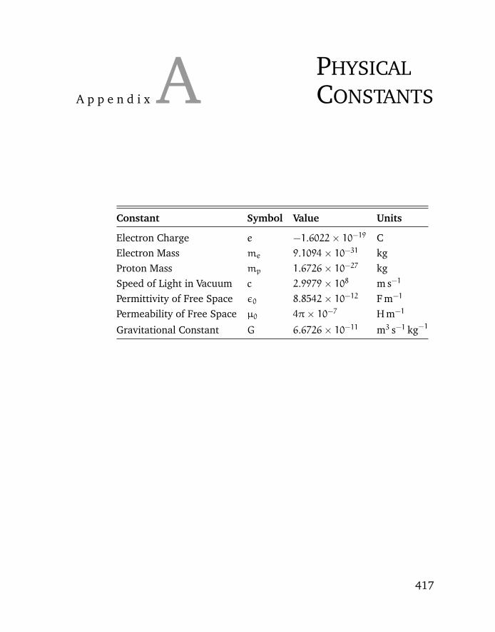
“appendixa” — 2007/11/29 — 16:42 — page 417 — #1
A p p e n d i x A PHYSICALCONSTANTS
Constant Symbol Value Units
Electron Charge e −1.6022× 10⁻¹⁹ CElectron Mass me 9.1094× 10⁻³¹ kgProton Mass mp 1.6726× 10⁻²⁷ kgSpeed of Light in Vacuum c 2.9979× 10⁸ m s−1
Permittivity of Free Space ε0 8.8542× 10⁻¹² F m−1
Permeability of Free Space µ0 4π× 10−7 H m−1
Gravitational Constant G 6.6726× 10⁻¹¹ m3 s−1 kg−1
417

“appendixa” — 2007/11/29 — 16:42 — page 418 — #2
“appendixb” — 2007/11/29 — 16:43 — page 419 — #1
A p p e n d i x BUSEFULVECTORIDENTITIES
Notation: a, b, c, d are general vectors; φ, ψ are general scalar fields;A, B are general vector fields.
a × (b × c) = (a · c) b − (a · b) c
(a × b) × c = (c · a) b − (c · b) a
(a × b) · (c × d) = (a · c) (b · d) − (a · d) (b · c)
(a × b) × (c × d) = (a × b · d) c − (a × b · c) d
∇ · ∇ × A = 0
∇ × ∇φ = 0
∇2A = ∇ (∇ · A) − ∇ × ∇ × A
∇(φψ) = φ∇ψ+ψ∇φ∇(A · B) = A × (∇ × B) + B × (∇ × A) + (A · ∇)B + (B · ∇)A
∇ · (φA) = φ∇ · A + A · ∇φ∇ · (A × B) = B · ∇ × A − A · ∇ × B
∇ × (φA) = φ∇ × A + ∇φ× A
∇ × (A × B) = A (∇ · B) − B (∇ · A) + (B · ∇)A − (A · ∇)B
419

“appendixb” — 2007/11/29 — 16:43 — page 420 — #2
“appendixc” — 2007/11/30 — 11:17 — page 421 — #1
A p p e n d i x C GAUSSIANUNITS
In 1960 physicists throughout the world adopted the so-called SI (shortfor the Systeme International) system of units , whose standard measuresof length, mass, time, and electric charge are the meter, kilogram, sec-ond, and coloumb, respectively. Nowadays, the SI system is employed,almost exclusively, in most areas of Physics. In fact, only one area ofPhysics has proved at all resistant to the adoption of SI units, andthat, unfortunately, is Electromagnetism, where the previous systemof units, the so-called Gaussian system, is still widely used. Inciden-tally, the standard units of length, mass, time, and electric charge inthe Gaussian system are the centimeter, gram, second, and statcoloumb,respectively.
Why would anyone wish to adopt a different set units in Electro-magnetism to that used in most other branches of Physics? The answeris that the laws of Electromagnetism look a lot prettier in the Gaussiansystem than in the SI system. In particular, there are no ε0 s and µ0 sin any of the formulae. In fact, within the Gaussian system, the onlynormalizing constant appearing in Maxwell’s equations is the velocityof light in vacuum, c. However, there is a severe price to pay for theaesthetic advantages of the Gaussian system.
Electromagnetic formulae can be converted from the SI to theGaussian system via the following transformations
ε0 → 1
4π, (C.1)
µ0 → 4π
c2, (C.2)
B → B
c. (C.3)
421
“appendixc” — 2007/11/30 — 11:17 — page 422 — #2
422 MAXWELL’S EQUATIONS AND THE PRINCIPLES OF ELECTROMAGNETISM
Transformation (C.3) also applies to quantities which are directlyrelated to magnetic field-strength, such as vector potential. Convertingelectromagnetic formulae from the Gaussian to the SI system (or anyother system) is far less straightforward. As an example of this, considerCoulomb’s law in SI units:
f2 =q1 q2
4πε0
r2 − r1|r2 − r1|3
. (C.4)
Employing the above transformation, this formula converts to
f2 = q1 q2r2 − r1
|r2 − r1|3(C.5)
in Gaussian units. However, applying the inverse transformation is prob-lematic. In Equation (C.5), the geometric 4π in the SI formula hascanceled with the 1/4π obtained from transforming ε0 to give unity.Unfortunately, it is not at all obvious that the inverse transformationshould generate a factor 4πε0 in the denominator. In order to understandthe origin of this difficulty, it is necessary to consider dimensionality.
There are four fundamental quantities in Electrodynamics: mass,length, time, and charge, denoted M, L, T , and Q, respectively. Eachof these quantities has its own particular units, since mass, length,time, and charge are fundamentally different (in a physical sense) fromone another. The units of a general physical quantity, such as force orcapacitance, can always be expressed as some appropriate power lawcombination of the four fundamental units, M, L, T , and Q. Now, alllaws of Physics, and all equations derived from such laws, must be dimen-sionally consistent (i.e., all terms on the left-hand and right-hand sidesmust possess the same power law combination of the four fundamentalunits) in order to ensure that the laws of Physics are independent of thechoice of units (which is, after all, completely arbitrary). Equation (C.4)makes dimensional sense because the constant ε0 possesses the unitsM−1 L−3 T2 Q2. Likewise, the Biot-Savart law only makes dimensionalsense because the constant µ0 possesses the unitsMLQ−2. On the otherhand, Eq. (C.5) does not make dimensional sense: i.e., the right-handside and the left-hand side appear to possess different units. In fact, wecan only reconcile Eqs. (C.4) and (C.5) if we divide the right-hand sideof (C.5) by some constant, 4πε0, say, with dimensions M−1 L−3 T2 Q2,which happens to have the numerical value unity for the particular choiceof units in the Gaussian scheme. Likewise, the Gaussian version of theBiot-Savart law contains a hidden constant with the numerical valueunity which nevertheless possesses dimensions. So, it can be seen that the
“appendixc” — 2007/11/30 — 11:17 — page 423 — #3
APPENDIX C GAUSSIAN UNITS 423
apparent simplicity of the equations of Electrodynamics in the Gaussianscheme is only achieved at the expense of wrecking their dimensionality.It is difficult to transform out of the Gaussian scheme because the afore-mentioned hidden constants, which lurk in virtually all of the equationsof Electromagnetism, do not necessarily have the value unity in otherschemes.

“appendixc” — 2007/11/30 — 11:17 — page 424 — #4
“appendixd” — 2007/11/30 — 11:48 — page 425 — #1
A p p e n d i x D FURTHERREADING
Foundations of Electromagnetic Theory, 3rd Edition, J.R. Reitz,F.J. Milford, R.W. Christy (Addison-Wesley, Reading MA, 1960).
Classical Electricity and Magnetism, 2nd Edition, W.K.H. Panofsky,M. Philips (Addison-Wesley, Reading MA, 1962).
Special Relativity, 2nd Edition, W. Rindler (Interscience, New York NY,1966).
Electromagnetic Fields and Waves, 2nd Edition, P. Lorrain, D.R. Corson(W.H. Freeman & Co., San Francisco CA, 1970).
Classical Electrodynamics, 2nd Edition, J.D. Jackson (John Wiley & Sons,New York NY, 1975).
Electromagnetism, I.S. Grant, W.R. Phillips (John Wiley & Sons, Chich-ester UK, 1975).
Essential Relativity: Special, General, and Cosmological, 2nd Rev. Edition,W. Rindler (Springer-Verlag, New York NY, 1980).
Introduction to Electrodynamics, 2nd Edition, D.J. Griffiths (Prentice-Hall, Englewood Cliffs NJ, 1989).
Classical Electromagnetic Radiation, 3rd Edition, M.A. Heald, J.B. Marion(Saunders College Publishing, Fort Worth TX, 1995).
Classical Electrodynamics, W. Greiner (Springer-Verlag, New York NY,1998).
425

“appendixd” — 2007/11/30 — 11:48 — page 426 — #2
“index” — 2007/12/27 — 18:20 — page 427 — #1
INDEX
3-acceleration, 3793-force, 393–3943-momentum, 392–3933-space, 3793-tensor, 367, 381–3823-vector field, 3783-vectors, 3784-acceleration, 379, 392–3934-force, 393–3944-momentum, 392–3934-tensor theory, 3674-tensor, 367–3694-vector, 367–369, 4034-velocity and 4-acceleration,
371–3724-velocity, 371–372, 379, 389,
392–394
AAcceleration 4-vector, 391Accelerated charges, 397–401
Field point, 397–398Virtual present radius vector,
401Source point, 397–398
Action-at-a-distance laws, 52Advanced potentials, 142–148
Green’s function, 142Feynman-Wheeler model,
143–145
Alternating current circuits,270–274
Resistors, 270Inductors, 270Capacitors, 270
Ampere, Marie Andre, 68Ampere’s law, 75–76, 118, 239,
250, 258, 277, 284–285Ampere’s circuital law, 79–85, 98,
116–117Ampere’s experiments, 68–71Angular distribution of radiation,
407–409Rate of radiation, 407–408
Angular momentumconservation, 294–297
Angular momentum density,294–295
Gauss’ law, 295Faraday’s law, 296
Amperian loop, 85Amperian magnetic field, 138Angular velocity, 17Anticommutative, 13Anticyclic permutation, 18Antisymmetric tensor, 389Arbitrarily shaped pulses, 131Arbitrary wave pulses, 131Arbitrary, 1Associative, 13
427
“index” — 2007/12/27 — 18:20 — page 428 — #2
428 INDEX
Associative, 6Astronomy, 128–129, 148Astrophysics, 409Axial tensors, 379
BBBC, 305Big Bang, 309Bio-Savart law, 95–97, 147,
138–139, 255–256,422–423
Biot, Jean Baptiste, 95Bound charge sheet, 220Bound charges, 216Boundary conditions on electric
field, 171–172Boundary value problems with
dielectrics, 220–226Laplace’s equation, 223
Bow waves, 140Box-car function, 59Breakdown, 173, 177Boundary value problems with
ferromagnets, 244–249Ferromagnetic sphere,
244–245Magnetic scalar potential,
245Laplace’s equation, 245–247Demagnetizing, 246Electromagnet, 249
CCapacitance, 2, 173–174Capacitors, 172–178, 270
Breakdown, 173, 177Capacitance, 173–174Conducting plates, 174Gauss’ law, 177
Cartesian frame, 351Cathode rays, 72, 74
Cauchy-Riemann relations,197–198
Central conductors, 347Charge density, 54Cherenkov radiation, 141–142Child-Langmuir law, 186Classic electromagnetism, 1, 52,
374Classical electron radius, 308,
411Classical electrostatics, 64Clausius-Mossotti relation,
230–234, 232Molecular polarizability, 231
Coefficient of transmission, 330Complex analysis, 195–202
Poisson’s equation, 195–196Laplace’s equation, 195Cauchy-Riemann relations,
197–198Conductors, 163, 165–172
Surface of, 166Uniform, 166Cavity, 166–167Faraday cage, 167Gaussian pill-box, 168–169,
171–172Gauss’ law, 166–169, 171
Coefficient of coupling, 262Coefficient of reflection, 329–330Coercivity, 242Collisions, 324–325Commutative, 6Computer networks, 274Conducting plates, 174Conductors, 2Conjugate, 363Conservative field, 31, 56Constitutive relation, 217Contraction from tensors, 362Contravariant tensor, 360–361
“index” — 2007/12/27 — 18:20 — page 429 — #3
INDEX 429
Coordinate approach, 6Coordinate-free fashion, 2Copper, 323–324Cosine rule of trigonometry, 11Cosmic microwave background,
309Coulomb gauge, 92–94, 99,
114–116Coulomb, Charles Augustine
de, 49Coulomb’s law, 49–54, 95, 100,
138–139, 147Covariant tensor, 360Curl, 38–43Curl theorem, 42Current density, 82Current density 4-vector,
372–373Current-carrying wire, 68, 76Cut-off frequency, 346Cyclotron frequency, 74, 319Cylindrical polar coordinates, 43
DD’Alembertian, 369, 374Decomposition of surface
integral, 24Decomposition of vector area, 40Del operator, 31Delta-function, 82, 135Demagnetizing, 246Diamagnetic, 240Dielectric constant of a gaseous
medium, 313–314Dielectric liquids in electrostatic
fields, 233–237Dielectric media, 215Dielectric tensor, 218Dielectrics, 2Differential scattering
cross-section, 308
Dirac delta-function, 60Dirac, Paul, 60Directed line element, 5Direction, 1Dispersion relation, 315Dispersion relation of a
collisional plasma, 324–326Collisions, 324–325
Dispersion relation of a plasma,314–318
Plasma frequency, 315Dispersion relation, 315Theory of Relativity, 315Group-velocity, 316Ionosphere, 318
Displacement current, 116–123Divergence, 32–36
Outward-pointing surfaceelement, 32
Flux of a vector field out of asmall box, 33
Divergence theorem, 34Divergence theorem, 34, 37,
292Dual electromagnetic field
tensor, 384–386Pseudo-4-tensor, 384–385Pseudo-3-tensor, 384–385Proper 3-vector, 385
Dust tail, 291
EEarnshaw’s theorem, 63–64Einstein summation convention,
291, 360Einstein’s Special Theory of
Relativity, 52Electric circuits, 2Electric dipole radiation, 306Electric displacement, 217Electric field, 53, 160

“index” — 2007/12/27 — 18:20 — page 430 — #4
430 INDEX
Electric scalar potential, 55, 91,112–113
Electric susceptibility andpermittivity, 217–218
Relative dielectric constant,217
Permittivity of free space, 217Electromagnetic energy tensor,
394–397Lorentz force density, 394–395Energy conservation equation,
396–397Momentum conservation
equation, 397Electromagnetic field tensor,
381–386, 395Proper 4-tensor, 381–382Pseudo-3-vector, 381–3823-tensor, 381–382Proper 3-tensor, 381–382
Electromagnetic momentum,287–291
Einstein’s thought experiment,287
Quantum theory, 289Radiation pressure, 290
Electromagnetic radiation, 121Electromagnetic spectrum, 129Electromagnetic waves, 124–131,
141, 148Electromagnetism, 63, 99, 107,
137, 145, 163, 255Electromotive force, 108Electrostatic energy, 157–165,
227Gauss’ theorem, 160Gauss’ law, 161
Electrostatic pressure, 170Electrostatics and magnetostatics,
97–101Electrostriction, 230
Electroweak force, 107Energy conservation, 283–287
Energy density, 283General electromagnetic field,
283Electromagnetic energy, 284Gauss’ theorem, 283–284Ampere’s law, 284–285Vector field theory, 285Faraday’s law, 285Poynting flux, 285–286
Energy conservation equation,396–397
Energy density, 160, 287Energy density within a dielectric
medium, 226–227Gauss’ theorem, 227
Equation of continuity, 36Equivalent circuit, 255Exponential functions, 206
FFar field region, 300Faraday cage, 167Faraday, Michael, 107, 116Faraday’s law, 107–112, 116,
147, 219, 262, 268, 285,296
Faraday rotation, 318–321Cyclotron frequency, 319Left-hand circularly polarized,
320Right-hand circularly
polarized, 320Linearly polarized
electromagnetic wave, 320Pulsars, 321
Ferromagnetism, 241–243Saturation magnetization, 242Hysteresis, 242Hysteresis loop, 242
“index” — 2007/12/27 — 18:20 — page 431 — #5
INDEX 431
Retentivity, 242Remanence, 242Coercivity, 242
Ferromagnetic sphere, 244–245Feynman, Richard P., 88, 143Feynman-Wheeler model,
143–145Field due to a moving charge,
388–391Instant of measurement, 390
Field point, 397–398Field theory, 1, 52, 61Field-lines, 53Force density within a dielectric
medium, 228–230Force of gravity, 31Force on a moving charge,
393–394Fourth-rank tensor, 377–378Fresnel’s equations, 333–335Frustrated total internal
reflection, 338–339Full-wave antenna, 280Fundamental tensor, 367
GGalilean transformation,
353–356Gauge condition, 375Gauge independent, 95Gauge invariance, 113, 374–375
Gauge condition, 375Lorentz gauge condition, 375
Gauge transformations, 92,113–116
Gauge invariance, 113Gauss theorem, 34Gauss’ law, 57–66, 98, 116, 161,
166–169, 171, 177,191–192, 195, 216–217,220, 295
Box-car function, 59One-dimensional spike
function, 59Generalized function, 60Dirac delta-function, 60Three-dimensional spike
function, 61One-dimensional
delta-function, 61Stationary charge
distributions, 63Earnshaw’s theorem, 63–64Gaussian surface, 64
Gauss’ theorem, 78, 84, 98, 111,117, 160, 180–183, 227,269, 283–284, 403
Gaussian pill-box, 168–169,171–172, 219, 244
Gaussian surface, 64Gaussian units, 421–423General electromagnetic field,
283General Lorentz transformation,
366Generalized function, 60Gradient, 28–32
Two-dimensional gradient, 28Gravity, 10, 49–50Green’s function, 67, 100,
132–135, 142Group-velocity, 316
HHalf-wave antenna, 279–280,
303Handedness convention, 379Heat, 164Helmholtz, Ferdinand von, 86Helmholtz’s theorem, 86–92, 97Hertzian dipole, 299–306
Electromagnetic energy, 299
“index” — 2007/12/27 — 18:20 — page 432 — #6
432 INDEX
Far field region, 300Radiation fields, 301Radiation resistance, 303Hertizian dipole antennas,
303–306Ohm’s law, 304Poynting flux, 305
Hertizian dipole antennas,303–306
High-energy physics, 141Hydrogen, 309–310Hysteresis, 242Hysteresis loop, 242
IImpedance, 272Inductance, 2, 255–261
Electromagnetism, 255Equivalent circuit, 255Inductance, 255Biot-Savart law, 255–256Mutual reluctance, 256Neumann formula, 257Self-inductance, 257Inductances of order one
micro-henry, 257–258Ampere’s law, 258Lenz’s law, 258–259Ohm’s law, 260
Inductances of order onemicro-henry, 257–258
Inductors, 270Inner multiplication of tensors,
362Input impedance, 277Instant of measurement,
390Interial confinement fusion,
291Interial mass, 392Intertial frame, 351
Inverse Lorentz transformation,356–357
Inverse-square force, 50Ionosphere, 318Isotherms, 30Isotropic gas pressure, 294
JJoined-up plan areas, 9
KKinetic energy, 56Kronecker delta symbol, 293,
360–362
LLaplace’s equation, 195Laplace’s equation, 90–91, 223,
245–247Laplacian, 36–38Larmor formula, 402–406
Gauss’ theorem, 403Larmor radius, 74–75Law of physics, 422–423Law of reflection, 332Le Chatelier’s principle, 109Left-hand circularly polarized,
320Lenz’s law, 109–110, 258–259,
262Lenzor tensor, 361Lienard-Wiechert potentials, 388Line integrals, 20–22Linearly polarized
electromagnetic wave, 320Lines of force, 36Lorentz factor, 357–359Lorentz force, 71–75
Lorentz force law, 72Lorentz force density, 394–395Lorentz formula, 129, 138
“index” — 2007/12/27 — 18:20 — page 433 — #7
INDEX 433
Lorentz gauge condition,115–116, 375
Lorentz transformation, 352–357,371, 378
Galilean transformation,353–356
Inverse Lorentztransformation, 356–357
Lorentz, Hendrik Antoon, 72Ludwig, Hermann, 86
MMagnetic energy, 249–251,
264–270Ohm’s law, 249–250Ampere’s law, 250Faraday’s law, 250Magnetostatic energy, 251Faraday’s law, 268Vector field theory, 269Gauss’ theorem, 269
Magnetic field lines, 70, 78Magnetic induction, 109Magnetic intensity, 239Magnetic materials, 2Magnetic monopoles, 76–79Magnetic permeability, 241Magnetic scalar potential, 245Magnetic susceptibility and
permeability, 240–241Paramagnetic, 240Diamagnetic, 240Magnetic permeability, 241Permeability of free space, 241
Magnetic vector potential, 91–94Gauge transformations, 92Coulomb gauge, 92–94
Magnetization, 237–240Magnetization current, 239Ampere’s law, 239Magnetic intensity, 239
Magnetization current, 239Magnetostatic energy, 251Magnetostatics, 99Maxwell stress tensor, 293Maxwell, James Clerk, 107, 116Method of images, 186–195
Poisson’s equation, 187Gauss’ law, 191–192, 195
Metric tensor, 367Microwaves, 128Milikan, robert, 73–74Mixed tensor, 361Molecular polarizability, 231Momentum conservation,
291–294Einstein summation
convention, 291Momentum flux density tensor,
291Divergence theorem, 292Vector field theory, 292Maxwell stress tensor, 293
Momentum conservationequation, 397
Momentum flux density tensor,291
Mutual inductance, 261–264Coefficient of coupling, 262Faraday’s law, 262Lenz’s law, 262
Mutual reluctance, 256Mutually repulsive elastic bands,
294
NNet rate of heat flow, 37Neumann formula, 257Newton, Isaac, 107Newton’s law of gravity, 49–50,
52Nitrogen, 311
“index” — 2007/12/27 — 18:20 — page 434 — #8
434 INDEX
Non-uniform dielectric constant,218–219
Normal reflection at a dielectricboundary, 326–330
Coefficient of reflection,329–330
Coefficient of transmission,330
NOVA experiment, 291
OOblique reflection at a dielectric
boundary, 330–336Plane of incidence, 331Law of reflection, 332Snell’s law of refraction,
332–336Fresnel’s equations, 333–335
Ohm’s law, 163–165, 249–250,260, 270, 304, 322
Ohm-meters, 164Oil drop experiment, 73–74One-dimensional delta-function,
61One-dimensional solutions of
Poisson’s equation,184–186
Child-Langmuir law, 186One-dimensional spike function,
59Optical coatings, 339–342Orested, Hans Christian, 68Orientation of loop, 38Orthogonal basis vectors, 7–8Outer multiplication of tensors,
362Oxygen, 311
PParallelogram, 5Paramagnetic, 240
Parity inversion, 378Permeability of free space, 70,
241Permittivity of free space, 217Perspex blocks, 141Phase-lag, 273Photons, 289Physics, 31Physical significance of tensors,
364–365Laws of physics, 365
Plane of incidence, 331Plasma frequency, 315Poisson’s equation, 66–67, 93–94,
99–100, 178, 187, 195–196,202–207
Green’s function, 67Polar coordinates, 43–48Polar sensors, 379Polarization, 215–217
Gauss’ law, 216–217Electric displacement, 217Constitutive relation, 217
Polarization, 225Polarization current, 237, 312Positive definite, 180Potential 4-vector, 374
Classical electromagnetism,374
Potential due to a moving charge,387–388
Lienard-Wiechert potentials,388
Potential formulation, 123–124Poynting flux, 285–286, 305,
397, 402Principal of virtue work, 170Principle of superposition, 53Propagation in dielectric
medium, 312–313Polarization current, 312
“index” — 2007/12/27 — 18:20 — page 435 — #9
INDEX 435
Propagation in a conductor,322–324
Ohm’s law, 322Propagation in a dielectric
medium, 312–313Proper 3-tensor, 381–382Proper 3-vector, 385Proper 4-tensor, 381–382Proper tensors, 379Proper time, 370–371
Time dilation effect, 371Lorentz transformation,
371Pseudo-3-tensor, 384–385Pseudo-3-vector, 381–382Pseudo-4-tensor, 384–385Pseudo-tensors, 379Pulsars, 321
QQuadruple electrostatic lenses,
199Qualified tensor, 361Quantum electrodynamics, 163Quantum electromagnetism, 52Quantum mechanics, 145Quantum Mechanics, 51, 60Quantum theory, 289Quotient rule, 362
RRadiation fields, 301Radiation losses, 406–407Radiation pressure, 290Radiation resistance, 303Radio waves, 128, 279–280Raising and lowering suffixes,
363Rayleigh scattering, 310–312
Simple harmonic oscillator,310
Rate of radiation, 407–408Real numbers, 5Rectangular wave-guide, 345Reflection at a metallic boundary,
342–343Relative dielectric constant, 217Relativistic particle dynamics,
391–392Relativity, 115Remanence, 242Renormalization, 163Resistivity, 164Resistors, 270Rest mass, 392Retarded fields, 145–148Retarded potentials, 136–142,
375–377Retarded time, 137Poisson’s equation, 136
Retarded time, 137Retentivity, 242Riemannian, 363Right-hand circularly
polarized, 320Right-handed rule for cross
products, 14Right-handed set, 13Rigid interial frames, 351Rotation, 15–17Rotation vector, 15–17Rotationally invariant, 97
SSalam, Abdus, 107Saturation magnetization, 242Savart, Felix, 95Scalar differential operator, 37Scalar potential, 115Scalar triple product, 17–18
Volume of vectorparallelepiped, 17
“index” — 2007/12/27 — 18:20 — page 436 — #10
436 INDEX
Second uniqueness theorem, 181Self-inductance, 257Separation of variables, 202–209
Poisson’s equation, 202–207Shockwaves, 140–141SI system, 422Silver, 342Sinusoidal oscillations, 131Skin-effect, 324Small angle rotations, 16Snell’s law of refraction,
332–336Solar System, 290Solar Wind, 291Solenoidal vector field, 36, 77Sonic booms, 140Source point, 397–398Space-time, 365–370
Standard coordinates,365–366
General Lorentztransformation, 366
Standard Lorentztransformation, 366
Fundamental tensor, 367Metric tensor, 3673-tensor, 3674-tensor, 367–3694-vector, 367–369
Special theory of relativity, 100Spherical polar coordinate
system, 44Spherical wavefronts, 140Standard coordinates, 365–366Standard Lorentz transformation,
366Standing waves, 317Stationary charge
distributions, 63Stokes’ theorem, 42, 56, 80–81,
83, 98
Strong force, 107Sun, 285, 309–311Supernova remnants, 129Superposable, 54Surface integrals, 24–26
Decomposition of surfaceintegral, 24
Synchrotron radiation, 409–412Classical electron radius, 411
TTaylor series, 146Telegrapher’s equations,
276–278Tensors, 359–364
Einstein summationconvention, 360
Covariant tensor, 360Contravariant tensor, 360–361Mixed tensor, 361Qualified tensor, 361Lenzor tensor, 361Theorem of tensor calculus,
361Tensors of the same type, 362Outer multiplication of tensors,
362Inner multiplication of tensors,
362Contraction from tensors, 362Quotient rule, 362
Tensors and pseudo-tensors,377–381
Fourth-rank tensor, 377–378Lorentz transformation, 378Parity inversion, 378Polar sensors, 379Pseudo-tensors, 379Axial tensors, 379Proper tensors, 379Handedness convention, 379
“index” — 2007/12/27 — 18:20 — page 437 — #11
INDEX 437
Tensors of the same type, 362Theorem of tensor calculus, 361Theory of Relativity, 315Thompson, J.J., 72Thompson scattering, 307–309
Differential scatteringcross-section, 308
Total scattering cross-section,308
Classical electron radius, 308Cosmic microwave
background, 309Thompson’s experiment, 72–73Three-dimensional
delta-function, 80Three-dimensional spike
function, 61Time constant, 260Time dilation effect, 371Total scattering cross-section, 308Transformation of velocities,
357–359Lorentz factor, 357–359Velocity addition formulae,
358Transformation of fields, 386–387Transmission lines, 274–280
Telegrapher’s equations,276–278
Computer networks, 274Input impedance, 277Ampere’s law, 277Half-wave antenna, 279–280Full-wave antenna, 280
Transverse electric, 345Tranverse electric and magnetic
fields, 344–345Cut-off frequency, 346Transverse electric, 345Tranverse electromagnetic, 347Central conductors, 347
Tranverse electromagnetic, 347Transverse magnetic, 345Transverse wave, 127Two-dimensional
delta-function, 80Two-dimensional gradient, 28
UUniform magnetic field, 75Uniqueness theorem, 99,
179–184Positive definite, 180Gauss’ theorem, 180–182Second uniqueness
theorem, 181
VVacuum diode, 185Vector addition theorem, 9Vector algebra, 5–8
Vectors, 5Movable, 5Parallelogram, 5Directed line element, 5Vector addition, 6–8Definition of a vector, 8
Vector calculus, 19–20Time derivative of vector, 19
Vector field theory, 2, 269, 285,292
Vector line integrals, 23–24Vector field, 23Scalar field, 23
Vector operator, 31Vector parallelogram, 14Vector product, 12–17Vector surface integrals, 26–27Vector triangle, 11Vector triple product, 18–19Velocity addition formulae,
358
“index” — 2007/12/27 — 18:20 — page 438 — #12
438 INDEX
Virtual present radius vector,401
Voltage, 108Volume, 17Volume integrals, 27
WWave fields, 148
Wave-guides, 343–348Tranverse electric and
magnetic fields, 344–345Rectangular wave-guide,
345Transverse magnetic, 345
Weinberg, Steve, 107Wheeler, John A., 143