MBP

MBP RF User Manual

MBP RF User Manual

Copyright Notice and Proprietary Information Copyright © Agilent Technologies, Inc. 2004, 2011. All rights reserved. This software and documentation contain confidential and proprietary information that is the property of Agilent Technologies, Inc. The software and documentation are furnished under a license agreement and may be used or copied only in accordance with the terms of the license agreement. No part of the software and documentation may be reproduced, transmitted, or translated, in any form or by a ny means, electronic, mechanical, manual, optical, or otherwise, without prior written permission of Agilent Technologies, Inc., or as expressly provided by the license agreement.

Right to Copy Documentation

The license agreement with Agilent Technologies permits licensee to make copies of the documentation for its internal use only. Each copy shall include all copyrights, trademarks, service marks, and proprietary rights notices, if any. Licensee must assign sequential numbers to all copies.

Disclaimer

AGILENT TECHNOLOGIES, INC. AND ITS LICENSORS MAKE NO WARRANTY OF ANY KIND, EXPRESS OR IMPLIED, WITH REGARD TO THIS MATERIAL, INCLUDING, BUT NOT LIMITED TO, THE IMPLIED WARRANTIES OF MERCHANTABILITY AND FITNESS FOR A PARTICULAR PURPOSE.

Registered Trademarks (®)

Agilent, Model Builder Program, MBP, Model Quality Assurance, MQA, Advanced Model Analysis, AMA, Proximity Quality Assurance, PQA are registered trademarks of Agilent Technologies, Inc.

MBP RF User Manual

Content 1. RF Data and Simulation ................................................................................................................... 1

1.1 Data Format .................................................................................................................. 1 1.2 S-parameter Simulation ................................................................................................ 2 1.3 Noise Simulation .......................................................................................................... 3 1.4 External Simulator ....................................................................................................... 3

2. Parameter Conversion ...................................................................................................................... 4 2.1 RF Parameters Supported in MBP ............................................................................... 4 2.2 Parameter Conversion in MBP ..................................................................................... 5

3. De-embedding .................................................................................................................................. 6 3.1 Open De-embedding Method ....................................................................................... 6 3.2 Short De-embedding Method ....................................................................................... 7 3.3 Open Short De-embedding Method ............................................................................. 7 3.4 Pad Open Short De-embedding Method [] ................................................................... 7 3.5 Open Short Thru De-embedding Method [] ................................................................. 9 3.6 Improved Open Short Thru De-embedding Method [] ................................................. 9 3.7 Cascaded Line Method ............................................................................................... 10

4. Customization by Script ................................................................................................................. 11 4.1 Customize Target ........................................................................................................ 11 4.2 Plot Model Parameters versus Instance Parameter ..................................................... 15

5. MBP Package and Solution ............................................................................................................ 17 5.1 Standard Inductor Package Introduction .................................................................... 17

5.1.1 Local Project ...................................................................................................... 18 5.1.2 Scalable Project .................................................................................................. 20

5.2 3-port Inductor ........................................................................................................... 22 References .............................................................................................................................................. 23

MBP RF User Manual

1. RF Data and Simulation

MBP provides complete RF modeling platform for various devices such as BJTs, MOSFETs, inductors, resistors, and capacitors. This document introduces the data structure.

1.1 Data Format

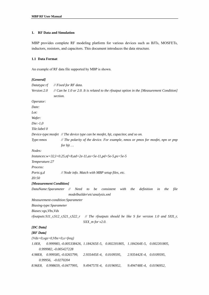
An example of RF data file supported by MBP is shown.

[General] Datatype:rf // Fixed for RF data. Version:2.0 // Can be 1.0 or 2.0. It is related to the rfoutput option in the [Measurement Condition]

section. Operator: Date: Lot: Wafer: Die:-1,0 Tile:label 0 Device-type:mosfet // The device type can be mosfet, bjt, capacitor, and so on. Type:nmos // The polarity of the device. For example, nmos or pmos for mosfet, npn or pnp

for bjt … Nodes: Instances:w=32,l=0.25,nf=8,ad=2e-11,as=5e-11,pd=5e-5,ps=5e-5 Temperature:27 Process: Ports:g,d // Node info. Match with MBP setup files, etc. Z0:50 [Measurement Condition] DataName:Sparameter // Need to be consistent with the definition in the file

modelbuilder\etc\analysis.xml Measurement-condition:Sparameter Biasing-type:Sparameter Biases:vgs,Vbs,Vds rfoutputs:S11_r,S12_r,S21_r,S22_r // The rfoutputs should be like S for version 1.0 and SXX_r,

SXX_m for v2.0. [DC Data] [RF Data] {Vds=0,vgs=0,Vbs=0,x=freq} 1.0E8, 0.999983, -0.005338426, 1.184265E-5, 0.002201805, 1.184264E-5, 0.002201805, 0.999982, -0.005427228 4.98E8, 0.999585, -0.0265799, 2.935445E-4, 0.0109595, 2.935442E-4, 0.0109595, 0.99956, -0.0270204 8.96E8, 0.998659, -0.0477995, 9.494757E-4, 0.0196952, 9.494748E-4, 0.0196952,

MBP RF User Manual

0.998578, -0.0485849 …… {Vds=0,vgs=0.25,Vbs=0,x=freq} 1.0E8, 0.999984, -0.005277605, 1.177794E-5, 0.002201806, 1.177793E-5, 0.002201806, 0.999982, -0.005427228 4.98E8, 0.999594, -0.0262772, 2.919413E-4, 0.0109595, 2.919411E-4, 0.0109595, 0.99956, -0.0270204 ……

There are four sections in an RF data file, namely:

[General] Describes general information such as device type, instance, temperature, and so on.

[Measurement Condition] The example describes the measurement condition of an S-parameter data file.

[DC Data] It is optional in the RF data file. The example does not contain DC data. [RF Data] The RF data is displayed in the following sequence: frequency, S11r, S11i, S12r,

S12i, S21r, S21i, S22r, S22i in every line. Note that currently MBP supports S-parameter or Y-parameter as the input data. If the raw data contains other kinds of parameters such as H or Z, convert them into S-parameter or Y-parameter first.

1.2 S-parameter Simulation

You can check the S-parameter simulation result with different plot styles, including Smith Chart, Polar

Chart, or simple X-Y graph. One example of inductor is shown in Figure 1.

Figure 1. S-parameter simulation

MBP RF User Manual

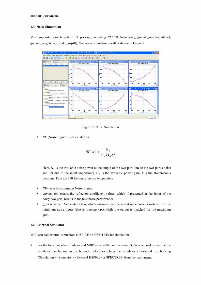
1.3 Noise Simulation

MBP supports noise targets in RF package, including NF(dB), NFmin(dB), gamma_opt(magnitude),

gamma_opt(phase) , and g_as(dB). One noise simulation result is shown in Figure 2.

Figure 2. Noise Simulation

NF (Noise Figure) is calculated as:

fkTGN

NF∆

+=0

1α

α

Here, Na is the available noise power at the output of the two-port (due to the two-port’s noise and not due to the input impedance). Ga is the available power gain. k is the Boltzmann’s constant. T0 is the 290 Kelvin reference temperature.

NFmin is the minimum Noise Figure. gamma_opt means the reflection coefficient values, which if presented at the input of the

noisy two-port, results in the best noise performance. g_as is named Associated Gain, which assumes that the in-out impedance is matched for the

minimum noise figure (that is, gamma_opt), while the output is matched for the maximum gain.

1.4 External Simulator

MBP can call external simulators (HSPICE or SPECTRE) for simulation.

For the local one (the simulator and MBP are installed on the same PC/Server), make sure that the

simulator can be run in batch mode before switching the simulator to external by choosing

“Simulation -> Simulator -> External HSPICE (or SPECTRE)” from the main menu.

MBP RF User Manual

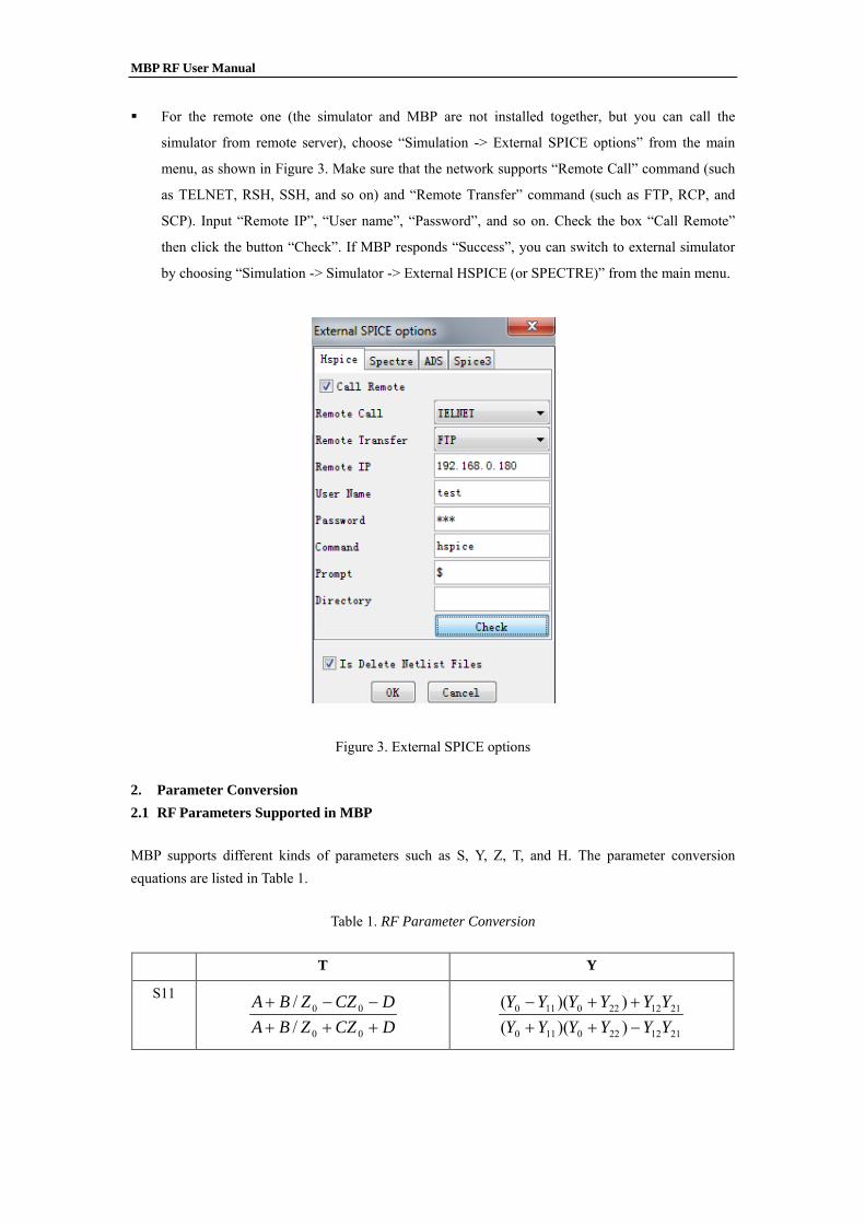
For the remote one (the simulator and MBP are not installed together, but you can call the

simulator from remote server), choose “Simulation -> External SPICE options” from the main

menu, as shown in Figure 3. Make sure that the network supports “Remote Call” command (such

as TELNET, RSH, SSH, and so on) and “Remote Transfer” command (such as FTP, RCP, and

SCP). Input “Remote IP”, “User name”, “Password”, and so on. Check the box “Call Remote”

then click the button “Check”. If MBP responds “Success”, you can switch to external simulator

by choosing “Simulation -> Simulator -> External HSPICE (or SPECTRE)” from the main menu.

Figure 3. External SPICE options

2. Parameter Conversion 2.1 RF Parameters Supported in MBP

MBP supports different kinds of parameters such as S, Y, Z, T, and H. The parameter conversion equations are listed in Table 1.

Table 1. RF Parameter Conversion

T Y

S11

DCZZBADCZZBA

+++−−+

00

00

//

2112220110

2112220110

))(())((

YYYYYYYYYYYY

−++++−

MBP RF User Manual

S12

DCZZBABCAD

+++−

00/)(2

2112220110

012

))((2

YYYYYYYY

−++−

S21

DCZZBA +++ 00/2

2112220110

021

))((2

YYYYYYYY

−++−

S22

DCZZBAACZZBD

+++−−+

00

00

//

2112220110

2112220110

))(())((

YYYYYYYYYYYY

−+++−+

Z H

S11

2112022011

2112022011

))(())((

ZZZZZZZZZZZZ

−++−+−

2112022011

2112022011

)/1)(()/1)((

HHZHZHHHZHZH

−++−+−

S12

2112022011

012

))((2

ZZZZZZZZ

−++ 2112022011

12

)/1)((2

HHZHZHH

−++

S21

2112022011

021

))((2

ZZZZZZZZ

−++ 2112022011

21

)/1)((2

HHZHZHH

−++

S22

2112022011

2112022011

))(())((

ZZZZZZZZZZZZ

−++−−+

2112022011

2112220011

)/1)(()/1)((

HHZHZHHHHZZH

−+++−−

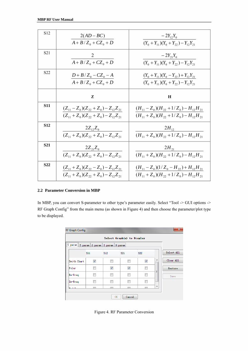
2.2 Parameter Conversion in MBP

In MBP, you can convert S-parameter to other type’s parameter easily. Select “Tool -> GUI options -> RF Graph Config” from the main menu (as shown in Figure 4) and then choose the parameter/plot type to be displayed.

Figure 4. RF Parameter Conversion

MBP RF User Manual

3. De-embedding

The De-embedding window can be enabled by choosing “Utilities -> Deembedding” from the main

menu. After loading the measurement data for different test structures (such as dut, open, and so on),

click the “Deembedding” button, as shown in Figure 5.

Figure 5. Load data for de-embedding

Choose the de-embedding method from the dropdown menu, as shown in Figure 6. Finally, click the “Run” button and save the de-embedding result.

Figure 6. Choose de-embedding method

Currently, there are seven de-embedding methodologies available in MBP. The subsequent subsections introduce them one by one.

3.1 Open De-embedding Method

Step1. dutdut YS → ; openopen YS →

MBP RF User Manual

Step2. opendutembde YYY −=−

Step3. embdeembde SY −− →

3.2 Short De-embedding Method

Step1. dutdut ZS → ; shortshort ZS →

Step2. shortdutembde ZZZ −=−

Step3. embdeembde SZ −− →

3.3 Open Short De-embedding Method

Step1. dutdut YS → ; openopen YS → ; shortshort YS →

Step2. opendut YYY −=1 ; openshort YYY −=2

Step3. 11 ZY → ; 22 ZY → ; 21 ZZZ embde −=−

Step4. emdeembde SZ −− →

3.4 Pad Open Short De-embedding Method [1]

Step1. dutdut YS → ; openopen YS → ; shortshort YS → ; padpad YS →

Step2. paddut YYY −=1 ; padshort YYY −=2 ; padopen YYY −=3

Step3. 11 ZY → ; 22 ZY → ; 33 ZY → ; 214 ZZZ −= ; 235 ZZZ −=

Step4. 44 YZ → ; 55 YZ → ; 54 YYY embde −=−

MBP RF User Manual

Step5. embdeembde SY −− →

The layout of test and dummy structure is shown in Figure 7, and the equivalent circuit is shown in Figure 8.

Figure 7. (a) Layout of the measured test structure consisting of a MOSFET surrounded by pads in GSG configuration

(b) Layouts of the dummy structures used to determine the pad parasitic effects

Figure 8. (a) General model for complete test-structure

(b) Assumed equivalent circuits for the pads, short, and open structures

MBP RF User Manual

3.5 Open Short Thru De-embedding Method [2]

Step1. ]2][1[]1][1[1 openopen YYG += ; ]2][1[]2][2[2 openopen YYG += ; ]2][1[3 openYG −=

11 ]1][1[]1][1[ GYY dutdut −= ; 2

1 ]2][2[]2][2[ GYY dutdut −=

Step2. )]2][2[

1]1][1[

1]2][1[

1(21

1shortshortthru YYY

Z −+= ;

)]2][2[

1]1][1[

1]2][1[

1(21

2shortshortthru YYY

Z +−= ;

)]2][2[

1]1][1[

1]2][1[

1(21

3shortshortthru YYY

Z ++−=

dutdut ZY 11 → ; 311 ]1][1[]1][1[ ZZZZ dutdut

s −−= ; 31 ]2][1[]2][1[ ZZZ dutdut

s −= ;

31 ]1][2[]1][2[ ZZZ dutdut

s −= ; 321 ]2][2[]2][2[ ZZZZ dutdut

s −−=

Step3. duts

duts YZ → ; 3]1][1[]1][1[ GYY dut

sdut

q −= ; 3]2][1[]2][1[ GYY duts

dutq += ;

3]1][2[]1][2[ GYY duts

dutq += ; 3]2][2[]2][2[ GYY dut

sdut

q −=

duts

dutq SY →

3.6 Improved Open Short Thru De-embedding Method [3]

Step1. ]2][1[]1][1[1 openopen YYG += ; ]2][1[]2][2[2 openopen YYG += ;

1

3 ]2][1[1

]1][1[1

21

−

+

−=

thruopen YYG

)]2][2[

1]1][1[

1]2][1[

1(21

211 GYGYY

Zshortshortthru −

−−

+−

=

MBP RF User Manual

)]2][2[

1]1][1[

1]2][1[

1(21

212 GYGYY

Zshortshortthru −

+−

−−

=

)]2][2[

1]1][1[

1]2][1[

1(21

213 GYGYY

Zshortshortthru −

+−

+=

−=

2

1

00

GG

YY measA

Step2.

+

+−=

323

331

ZZZZZZ

ZZ AB

Step3.

−

−−=

33

33

GGGG

YY BDUT

3.7 Cascaded Line Method

Step1. dutdut YS → ; openopen YS → ; thruthru YS →

Step2. opendutdutopen YYY −= ; openthruthruopen YYY −=

Step3. dutopendutopen AY → , where 21 sindsdutopen AAAA =

Step4. 21

,,2122

,11

,,2122

,11

),1(),1(

0

−−−+

=openthruopenthru

openthruopenthru

SSSS

ZZ

21

,,2122

,,1121

,,2122

,,11

,,212

,,112

])1[(])1[(

1

openthruopenthruopenthruopenthru

openthruopenthru

SSSS

SSD−−−+

+−=

lDD

2

)11ln(

−+

=λ

MBP RF User Manual

=

)cosh()sinh(

)sinh()cosh(

2,12,1

2,12,1

2,1 lZ

llZl

As γγ

γγ

Step5. 12,

11

−−= sopendutsInd AAAA

indind SA →

Some parameters should be set to reasonable values before de-embedding: L1, L2 are the length of extending lines (as shown in Figure 9) that should be de-embedded from the initial data. L is the total length of the transmission line in the thru de-embedding structure. Z0 is the characteristic impedance of test system (Its default value is 50).

Figure 9. Extending lines de-embedding

4. Customization by Script 4.1 Customize Target

MBP defines many useful targets for RF Application in default package, such as Leff, Reff, Q for

inductor model and ft, fmax for MOSFET model. Additionally, MBP supports user-defined targets. For

example, take the implementation of Leff, Reff, Q.

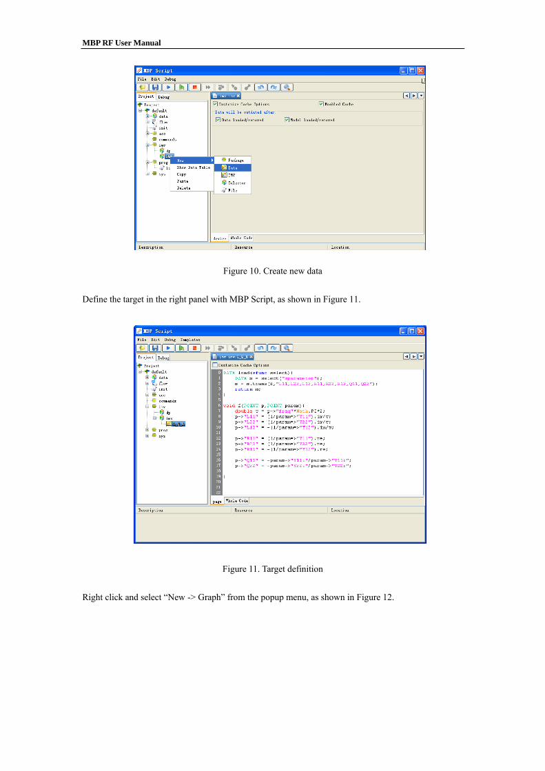
Select “Script -> Script Project” from the main menu. In the left Project panel, select default -> imv ->

imv. Right click and choose “New -> Data” in the popup menu, as shown in Figure 10.

MBP RF User Manual

Figure 10. Create new data

Define the target in the right panel with MBP Script, as shown in Figure 11.

Figure 11. Target definition

Right click and select “New -> Graph” from the popup menu, as shown in Figure 12.

MBP RF User Manual

Figure 12. Create new graph

Edit the property of graph. Input the information such as “Title”, “Axis[x]”, “Axis[y]” in the

GRAPH_PROP tab, as shown in Figure 13.

Figure 13. Edit graph property

Select default -> sys -> gui -> navigator in the left Project panel. Right click and choose “New ->

Navigator” from the popup menu, as shown in Figure 14.

MBP RF User Manual

Figure 14. Add new navigator

Select the navigator. Right click and choose “New -> Graph” from the popup menu, as shown in Figure 15.

Figure 15. Add Graph to the Navigator

Click the run button. The new navigator is shown in the main GUI of MBP. Two example results are

shown in Figure 16 and Figure 17, respectively.

MBP RF User Manual

Figure 16. New navigator L_Q_R in GUI

Figure 17. New navigator SweepR in GUI

4.2 Plot Model Parameters versus Instance Parameter

Choose "Script -> Script Project" from the main menu to pop up the MBP Script interface. Define the data (default -> imv > imv -> Target -> Cox1), as shown in Figure 18. This example can be loaded by choosing “Model -> Select Model -> RF -> standard -> scalable” from the main menu.

MBP RF User Manual

Figure 18. Show data table

Define the plot (default -> imv > imv -> Target -> Cox1 -> Cox1), as shown in Figure 19. Select the targets for X, Y, and P axes.

Figure 19. Define plot

Add the plot to the navigator (default -> sys > gui -> navigator), shown in Figure 20.

MBP RF User Manual

Figure 20. Add plot to navigator

Load the initial scalable model first and load point models from “Model -> Local Model Manager”. Select the navigator from the “Navigator” menu, as shown in Figure 21.

Figure 21. Select navigator

5. MBP Package and Solution 5.1 Standard Inductor Package Introduction

MBP provides inductor package for generic usage of standard inductor modeling. The default inductor

MBP RF User Manual

model has 2-pi structure. Its equivalent circuit is shown in Figure 22.

Figure 22. Equivalent circuit of the inductor with 2-pi structure

The definitions of Leff, Reff, and Q are shown:

FreqPIY

imagL

××=

2

)1(11

11 ; FreqPI

Yimag

L××

=2

)1(22

22 ; FreqPIY

imagL

××

−=

2

)1(12

12

FreqPIY

realR

××=

2

)1(11

11 ; FreqPI

Yreal

R××

=2

)1(22

22 ; FreqPIY

realR

××

−=

2

)1(12

12

)()(

11

1111 Yreal

YimagQ = ; )()(

22

2222 Yreal

YimagQ = ;

For standard inductor model extraction, there are two projects in MBP inductor package: local project

and scalable project.

5.1.1 Local Project

In the local project, each device is extracted by a point model. You can open it by choosing “Mode ->

Select Model -> RF -> inductor -> standard -> local” from the main menu. The flow is displayed. Click

the “Run” icon to run the flow from “InitPath_1”. A window pops up and you should input the

following information, as shown in Figure 23.

1) InitialModel: to set initial model name.

2) Measurement: to set measurement data folder.

3) LocalModel: to set folder for all the generated point models.

MBP RF User Manual

Figure 23. Set initialized condition

After entering the information, MBP runs the flow automatically. It loads one device every time, then

generates the corresponding point model. The fitting results are shown in Figure 24.

Figure 24. Generation of point models

All the point models are saved automatically in the target folder. If the point model is not good, it can

be due to the boundary of parameters or the initial model. You can extend the boundary or select the

point model of similar size as the initial model, and run the flow again.

MBP RF User Manual

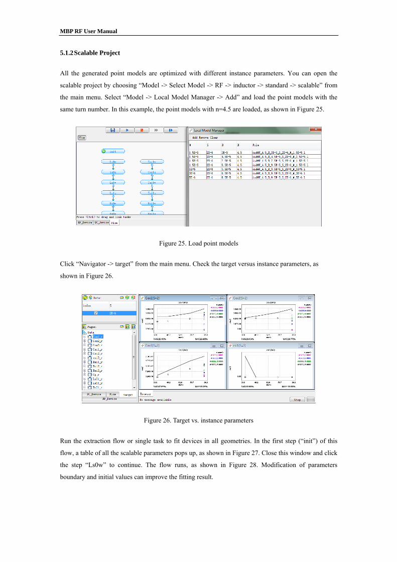
5.1.2 Scalable Project

All the generated point models are optimized with different instance parameters. You can open the

scalable project by choosing “Model -> Select Model -> RF -> inductor -> standard -> scalable” from

the main menu. Select “Model -> Local Model Manager -> Add” and load the point models with the

same turn number. In this example, the point models with n=4.5 are loaded, as shown in Figure 25.

Figure 25. Load point models

Click “Navigator -> target” from the main menu. Check the target versus instance parameters, as

shown in Figure 26.

Figure 26. Target vs. instance parameters

Run the extraction flow or single task to fit devices in all geometries. In the first step (“init”) of this

flow, a table of all the scalable parameters pops up, as shown in Figure 27. Close this window and click

the step “Ls0w” to continue. The flow runs, as shown in Figure 28. Modification of parameters

boundary and initial values can improve the fitting result.

MBP RF User Manual

Figure 27. Scalable parameter table

Figure 28. Run extraction flow

Save the scalable model when all the tasks are completed. There are some requirements for the name of

the scalable model. If the point models’ turn number is 4.5, the scalable model should be named as

“4p5.l”.

Clear the point models in the local model manager and other load point models with different turn number, for example, the point models with n=3.5. Repeat the steps and save the generated scalable model as “3p5.l”.

Finally, run the task named “mergeModel” to merge the scalable models. Select all the scalable models with different turn numbers, as shown in Figure 29. Save the final model.

MBP RF User Manual

Figure 29. Merge the model

Tips:

Pay attention to the boundary of parameters. They are varied for different data. Deselect the “bad” point model that deviates from the line. If the result is not acceptable, the scalable function should be modified for better result. If the number of point models with turn number is high, it is given preference over other point

models with turn number. For example, there are eight-point models whose turn number is 4.5 and seven-point models whose turn number is 3.5. In this case, select point models whose turn number is 4.5 prior to 3.5.

5.2 3-port Inductor

Choose “Model -> Select Model -> RF -> inductor -> 3port” from the main menu to open the default

project. Check the default 3-port inductor model by clicking the “Edit Model” icon , as shown in

Figure 30. You can load the user-defined model freely.

Figure 30. Default 3-port inductor model

MBP RF User Manual

Choose “File -> Data -> Load” to load the measurement data. The demo data is located under

“modelbuilder\demo\RF\inductor\3port”. The RF data conversion window can be enabled by choosing

“Tool -> GUI Options -> RF Graph Config” from the main menu, as shown in Figure 31.

Figure 31. RF Graph Config

References

[1] Reydezel Torres-Torres,”Analytical Model and Parameter Extraction to Account for the Pad Parasitics in RF-CMOS“IEEE TRANSACTIONS ON ELECTRON DEVICES, VOL. 52, NO. 7, JULY 2005 [2] Hanjin Cho and Dorothea E. Burk,” A Three-Step Method for the De-Embedding of High- Frequency S-Parameter Measurements” IEEE TRANSACTIONS ON ELECTRON DEVICES. VOL. 38. NO. 6, JUNE 1991 [3] Ewout P. Vandamme, Dominique M. M.-P. Schreurs, and Cees van Dinther,” mproved Three-Step De-Embedding Method to Accurately Account for the Influence of Pad Parasitics in Silicon On-Wafer RF Test-Structures” IEEE TRANSACTIONS ON ELECTRON DEVICES, VOL. 48, NO. 4, APRIL 2001