mcgraw-hill/irwin © the mcgraw-hill companies, inc., 2003 6.1 transportation and assignment models
TRANSCRIPT

© The McGraw-Hill Companies, Inc., 20036.1McGraw-Hill/Irwin
Transportation and
Assignment Models

© The McGraw-Hill Companies, Inc., 20036.2McGraw-Hill/Irwin
Outline
• Network models in general– Transportation, Assignment and Transshipment models belong to a
special class of linear programming problems called network flow problems
• Characteristics of Transportation models
• Characteristics of Assignment models
• Variations on a theme
© The McGraw-Hill Companies, Inc., 20036.3McGraw-Hill/Irwin
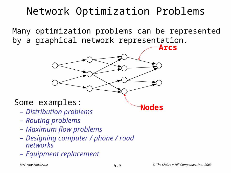
Network Optimization Problems
Many optimization problems can be represented by a graphical network representation.
Some examples:– Distribution problems– Routing problems– Maximum flow problems– Designing computer / phone / road networks– Equipment replacement
Arcs
Nodes
© The McGraw-Hill Companies, Inc., 20036.4McGraw-Hill/Irwin
Transportation problem• Frequently arises in planning for distribution of goods and
services from several supply locations to several demand locations.– Examples?
• Characteristics (typical)– Quantity of goods available at each supply location is limited.– Quantity of goods needed at each of several demand locations is known.– Usual objective of a transportation problem is to minimize the cost of shipping goods from the origins
to the destinations.
• Variations on the Transportation Problem theme– Total supply not equal to total demand.– Maximization objective function.– Route capacities or route minimums.– Unacceptable routes.
© The McGraw-Hill Companies, Inc., 20036.5McGraw-Hill/Irwin
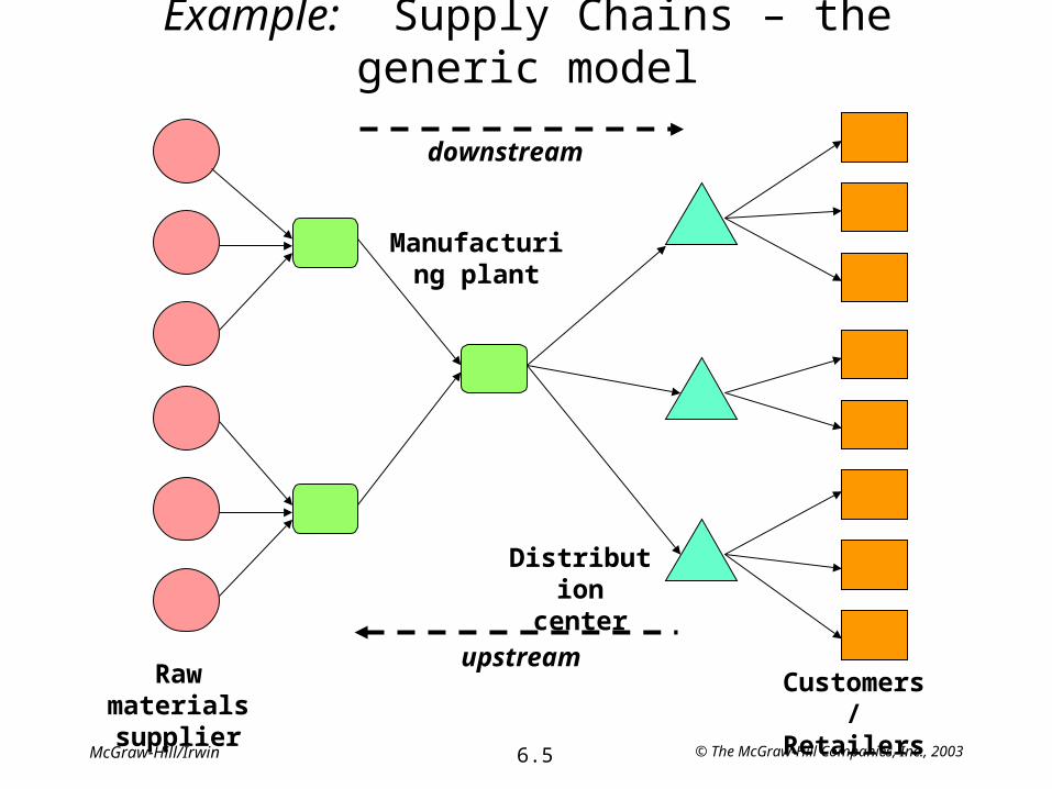
Example: Supply Chains – the generic model
Raw materials supplier
Manufacturing plant
Distribution center
Customers/
Retailers
upstream
downstream

© The McGraw-Hill Companies, Inc., 20036.6McGraw-Hill/Irwin
Example: Forest industry supply chain
Wagner, H.M. (1975). Principles of Operations Research 2nd ed. Englewood Cliffs NJ: Prentice-Hall

© The McGraw-Hill Companies, Inc., 20036.7McGraw-Hill/Irwin
Assumptions of Transportation Problems
• The Requirements Assumption– Each source has a fixed supply of units, where this entire supply must be distributed
to the destinations.– Each destination has a fixed demand for units, where this entire demand must be
received from the sources.
• The Feasible Solutions Property– A transportation problem will have feasible solutions if and only if the sum of its
supplies equals the sum of its demands.
• The Cost Assumption– The cost of distributing units from any particular source to any particular destination is
directly proportional to the number of units distributed.– This cost is just the unit cost of distribution multiplied by the number of units
distributed.

© The McGraw-Hill Companies, Inc., 20036.8McGraw-Hill/Irwin
The network for a transportation problem
Variable costs - cij
Quantities - xij
Dem
an
ds - D
j
Cap
aci
ties
- K
i
Region 1
Region 2
Region 4
Region 3
Plant 1
Plant 2
Plant 3
The Decision Variable
© The McGraw-Hill Companies, Inc., 20036.9McGraw-Hill/Irwin
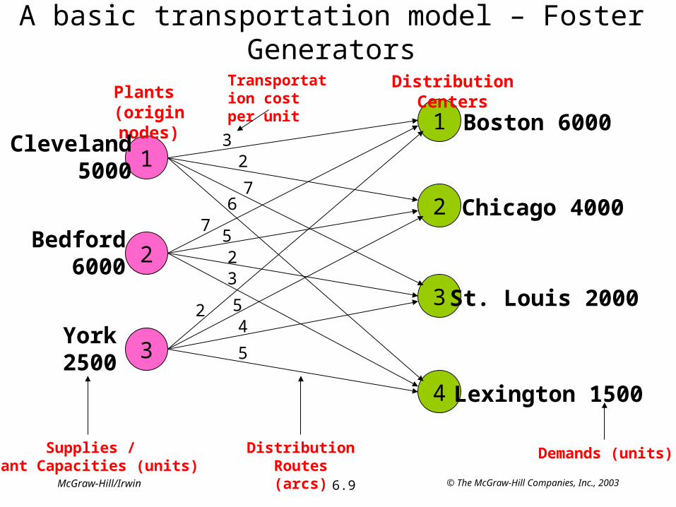
A basic transportation model – Foster Generators
2
3
1
1
2
3
4
32
76
4
5
32
2
7
5
5
Transportation cost per unit
Plants (origin nodes)
Distribution Centers
Chicago 4000
St. Louis 2000
Bedford6000
Boston 6000
Distribution Routes (arcs)
Lexington 1500
York2500
Cleveland5000
Supplies /Plant Capacities (units)
Demands (units)
© The McGraw-Hill Companies, Inc., 20036.10McGraw-Hill/Irwin
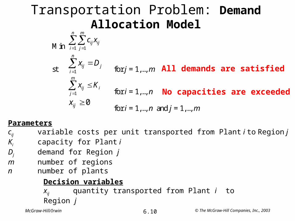
Min
n
i
m
jijij xc
1 1
st
n
ijij Dx
1 for j = 1,.., m
m
jiij Kx
1 for i = 1,.., n
0ijx for i = 1,.., n and j = 1,.., m
Parameters: cij variable costs per unit transported from plant i to region j Ki capacity for plant i Dj demand for region j m number of regions n number of plants
Decision variables: xij quantity transported from plant i to region j
Parameterscij variable costs per unit transported from Plant i to Region jKi capacity for Plant iDj demand for Region jm number of regionsn number of plants
Decision variablesxij quantity transported from Plant i to Region j
All demands are satisfied
No capacities are exceeded
Transportation Problem: Demand Allocation Model
© The McGraw-Hill Companies, Inc., 20036.11McGraw-Hill/Irwin
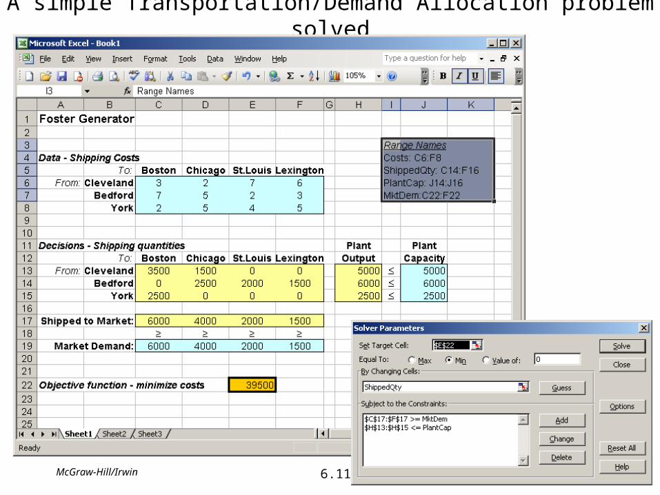
A simple Transportation/Demand Allocation problem solved

© The McGraw-Hill Companies, Inc., 20036.12McGraw-Hill/Irwin
The Capacitated Plant Location Model (CPLM)
• Open/Closed
• Fixed costs
• Capacities
• Variable costs
• Quantities
• Demands
Ware-house 1
Ware-house 2
Ware-house 3
Plant 1
Plant 2
Plant 3

© The McGraw-Hill Companies, Inc., 20036.13McGraw-Hill/Irwin
The Capacitated Plant Location Model (CPLM)
Min
n
i
n
i
m
jijijii xcyf
1 1 1
st
m
jijii xyK
1
0 for i = 1,.., n
n
iijj xD
1
0 for j = 1,.., m
1/0iy for i = 1,.., n 0ijx
for i = 1,.., n and j = 1,.., m
Decision variablesyi binary variable indicating whether Plant i should be open (1) or closed (0)xij quantity transported from Plant i to Region j
ParametersFi fixed costs for Plant icij variable costs per unit transported from Plant i to Region jKi capacity for Plant iDj demand for Region jm number of regionsn number of potential plants

© The McGraw-Hill Companies, Inc., 20036.14McGraw-Hill/Irwin
The CPLM with single sourcing
Ware-house 1
Ware-house 2
Ware-house 3
Plant 1
Plant 2
Plant 3
• Variable costs
• Open/Closed
• Fixed costs
• Capacities
• Assigning plants to warehouses
• Demands

© The McGraw-Hill Companies, Inc., 20036.15McGraw-Hill/Irwin
The CPLM with single sourcing
Min
n
i
n
i
m
jijijjii xcDyf
1 1 1
st
n
iijx
1
1 for j = 1,.., m
ii
n
jijj yKxD
1 for i = 1,.., n
1/0iy for i = 1,.., n 1/0ijx
for i = 1,.., n and j = 1,.., m
ParametersFi fixed costs for Plant icij variable costs per unit transported from Plant i to Region jKi capacity for Plant iDj demand for Region jm number of regionsn number of potential plants
Decision variablesyi binary variable indicating whether Plant i should be open(1) or
closed (0)xij binary variable indicating whether Plant i should supply market in Region j

© The McGraw-Hill Companies, Inc., 20036.16McGraw-Hill/Irwin
Transshipment model with sourcing
Market1
Market1
Market2
Market2
Market3
Market3
Plant 1Plant 1Supplier
1Supplier
1
Supplier2
Supplier2
Plant 2Plant 2
Plant 3Plant 3
Ware-house 1Ware-
house 1
Ware-house 2Ware-
house 2
Variable costs
Open/ ClosedQuantities
Capacities
Fixed costs
Demands
Open/ Closed
Quantities Quantities
Variable costs
Variable costs
Fixed costs
Capacities
Capacities
(Combines plant location, warehouse location and sourcing)

© The McGraw-Hill Companies, Inc., 20036.17McGraw-Hill/Irwin
Transshipment model with sourcing
t
e
m
j
ejej
n
i
t
e
ieie
l
h
n
i
hihi
t
e
ee
n
i
ii xcxcxcyfyF1 11 11 111
min
subject to:
0,,},1,0{,
0
0
1
1
11
1
1 1
1
hiieejei
j
t
e
ej
ee
m
j
ej
m
j
ej
n
i
ie
ii
t
e
ie
l
h
t
e
iehi
n
i
hhi
xxxyy
Dx
yWx
xx
yKx
xx
Sx
for i = 1, 2, 3, …, n
for i = 1, 2, 3, …, n
for e = 1, 2, 3, …, t
for e = 1, 2, 3, …, t
for j = 1, 2, 3, …, m
for h = 1, 2, 3, …, l
Warehouse capacity constraint
Warehouse flow balance
Market satisfaction
Plant flow balance
Plant capacity constraint
Source capacity constraint
Warehouse fixed
costs
Supplier-Plant
variable costs
Plant-Warehouse
variable costs
Warehouse-Market variable
costs
Plant fixed costs
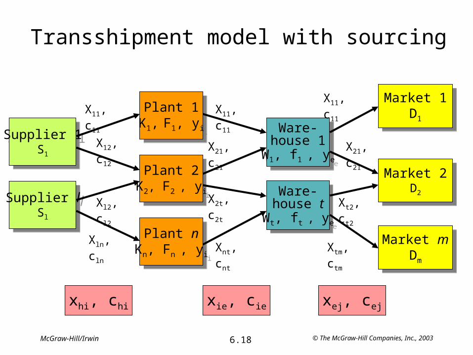
© The McGraw-Hill Companies, Inc., 20036.18McGraw-Hill/Irwin
Transshipment model with sourcing
Market 1D1
Market 1D1
Market 2D2
Market 2D2
Market mDm
Market mDm
Plant 1K1, F1, yi
Plant 1K1, F1, yi
Supplier 1S1
Supplier 1S1
Supplier lSl
Supplier lSl
Plant 2K2, F2 , yi
Plant 2K2, F2 , yi
Plant nKn, Fn , yi
Plant nKn, Fn , yi
Ware-house 1W1, f1 , ye
Ware-house 1W1, f1 , ye
Ware-house tWt, ft , ye
Ware-house tWt, ft , ye
X12, c12
Xtm, ctm
X21, c21
Xt2, ct2
X11, c11X11, c11
Xl2, cl2
Xln, cln
X11, c11
X21, c21
X2t, c2t
Xnt, cnt
xie, cie xej, cejxhi, chi

© The McGraw-Hill Companies, Inc., 20036.19McGraw-Hill/Irwin
Transshipment model with sourcing
Parametersm number of markets or demand pointsn number of potential plant or factory
locationsl number of supplierst number of potential warehouse locations
Dj annual demand from customer j
Ki potential capacity of plant at site i
Sh supply capacity at supplier h
We potential warehouse capacity at site e
Fi fixed cost of locating a plant at site i
fe fixed cost of locating a warehouse at site e
chi cost of shipping one unit from supply source h to plant i
cie cost of producing and shipping one unit from plant i to warehouse e
cej cost of shipping one unit from warehouse e to customer j
Decision variables
yi 1 if plant is located at site i, 0 otherwise
ye 1 if warehouse is located at site e, 0 otherwise
xei quantity shipped from warehouse e to market j
xie quantity shipped from plant at site i to warehouse e
xhi quantity shipped from supplier h to plant at site i

© The McGraw-Hill Companies, Inc., 20036.20McGraw-Hill/Irwin
The Assignment Problem• Arises in a variety of decision making situations:
– Jobs to machines– Agents to tasks– Sales personnel to sales territories– Contracts to bidders– Spacecraft to planetary missions– Nuclear warheads to targets
• Distinguishing feature of the basic assignment problem – One agent is assigned to one and only one task
• We seek a set of assignments that optimizes a stated objective– Minimize costs– Minimize time– Maximize profit– Maximize observation time– Maximize damage– …etc.

© The McGraw-Hill Companies, Inc., 20036.21McGraw-Hill/Irwin
An Assignment Problem – Fowle Marketing
2
3
1
1
2
3
1015
9
3
18
5
6
9
14
Completion time in days
Project leaders (origin nodes)
Clients (destination
nodes)
Client 2 - 1
Client 3 - 1
Kari - 1
Client 1 - 1
Possible assignments
(arcs)
Gudmund - 1
Terry - 1
Supplies
Demands

© The McGraw-Hill Companies, Inc., 20036.22McGraw-Hill/Irwin
The Assignment Problem
Parameterscij cost of assigning Agent i to Task jm number of Agentsn number of Tasks
Decision variablesxij assignment of Agent i to Task j, 0 if not assigned, 1 if assigned

© The McGraw-Hill Companies, Inc., 20036.23McGraw-Hill/Irwin
A simple Assignment Problem solved
© The McGraw-Hill Companies, Inc., 20036.24McGraw-Hill/Irwin
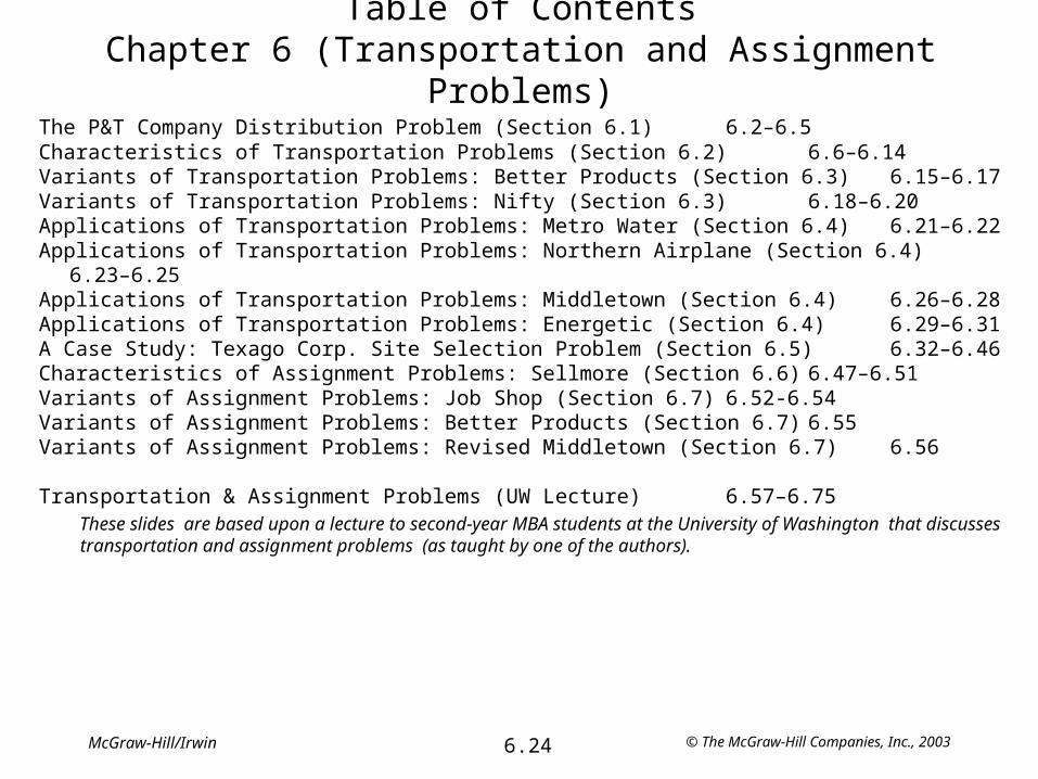
Table of ContentsChapter 6 (Transportation and Assignment
Problems)The P&T Company Distribution Problem (Section 6.1) 6.2–6.5Characteristics of Transportation Problems (Section 6.2) 6.6–6.14Variants of Transportation Problems: Better Products (Section 6.3) 6.15–6.17Variants of Transportation Problems: Nifty (Section 6.3) 6.18–6.20Applications of Transportation Problems: Metro Water (Section 6.4)
6.21–6.22Applications of Transportation Problems: Northern Airplane (Section 6.4)
6.23–6.25Applications of Transportation Problems: Middletown (Section 6.4) 6.26–6.28Applications of Transportation Problems: Energetic (Section 6.4) 6.29–6.31A Case Study: Texago Corp. Site Selection Problem (Section 6.5) 6.32–6.46Characteristics of Assignment Problems: Sellmore (Section 6.6) 6.47–6.51Variants of Assignment Problems: Job Shop (Section 6.7) 6.52-6.54Variants of Assignment Problems: Better Products (Section 6.7) 6.55Variants of Assignment Problems: Revised Middletown (Section 6.7)
6.56
Transportation & Assignment Problems (UW Lecture) 6.57–6.75These slides are based upon a lecture to second-year MBA students at the University of Washington that discusses transportation and assignment problems (as taught by one of the authors).

© The McGraw-Hill Companies, Inc., 20036.25McGraw-Hill/Irwin
P&T Company Distribution Problem
CANNERY 1 Bellingham
CANNERY 2 Eugene
WAREHOUSE 1 Sacramento
WAREHOUSE 2 Salt Lake City
WAREHOUSE 3 Rapid City
WAREHOUSE 4 Albuquerque
CANNERY 3 Albert Lea

© The McGraw-Hill Companies, Inc., 20036.26McGraw-Hill/Irwin
Shipping Data
Cannery OutputWarehous
eAllocation
Bellingham75
truckloadsSacramento
80 truckloads
Eugene125
truckloadsSalt Lake City
65 truckloads
Albert Lea100
truckloadsRapid City
70 truckloads
Total300
truckloadsAlbuquerque
85 truckloads
Total300
truckloads
© The McGraw-Hill Companies, Inc., 20036.27McGraw-Hill/Irwin
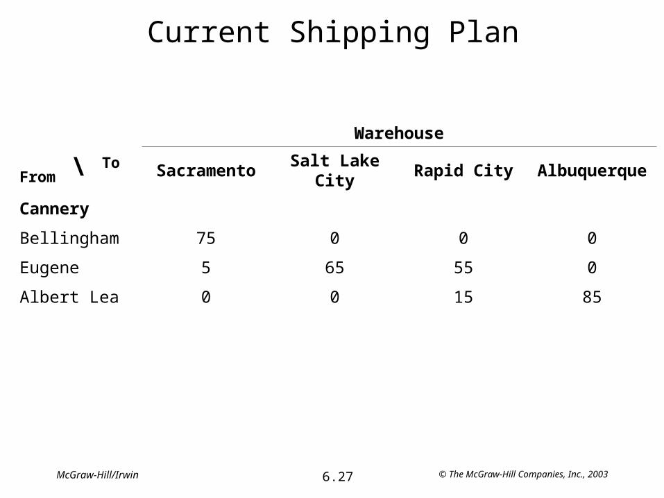
Current Shipping Plan
Warehouse
From \ To SacramentoSalt Lake
CityRapid City
Albuquerque
Cannery
Bellingham 75 0 0 0
Eugene 5 65 55 0
Albert Lea 0 0 15 85

© The McGraw-Hill Companies, Inc., 20036.28McGraw-Hill/Irwin
Shipping Cost per Truckload
Warehouse
From \ To Sacramento
Salt Lake City
Rapid CityAlbuquerq
ue
Cannery
Bellingham $464 $513 $654 $867
Eugene 352 416 690 791
Albert Lea 995 682 388 685
Total shipping cost = 75($464) + 5($352) + 65($416) + 55($690) + 15($388) + 85($685)
= $165,595

© The McGraw-Hill Companies, Inc., 20036.29McGraw-Hill/Irwin
Terminology for a Transportation Problem
P&T Company Problem
Truckloads of canned peas
Canneries
Warehouses
Output from a cannery
Allocation to a warehouse
Shipping cost per truckload from a cannery to a warehouse
General Model
Units of a commodity
Sources
Destinations
Supply from a source
Demand at a destination
Cost per unit distributed from a source to a destination

© The McGraw-Hill Companies, Inc., 20036.30McGraw-Hill/Irwin
Characteristics of Transportation Problems
• The Requirements Assumption– Each source has a fixed supply of units, where this entire supply must be
distributed to the destinations.– Each destination has a fixed demand for units, where this entire demand must be
received from the sources.
• The Feasible Solutions Property– A transportation problem will have feasible solutions if and only if the sum of its
supplies equals the sum of its demands.
• The Cost Assumption– The cost of distributing units from any particular source to any particular
destination is directly proportional to the number of units distributed.– This cost is just the unit cost of distribution times the number of units distributed.

© The McGraw-Hill Companies, Inc., 20036.31McGraw-Hill/Irwin
The Transportation Model
• Any problem (whether involving transportation or not) fits the model for a transportation problem if:1. It can be described completely in terms of a table like Table 6.5 that
identifies all the sources, destinations, supplies, demands, and unit costs, and…
2. Satisfies both the requirements assumption and the cost assumption.
• The objective is to minimize the total cost of distributing the units.
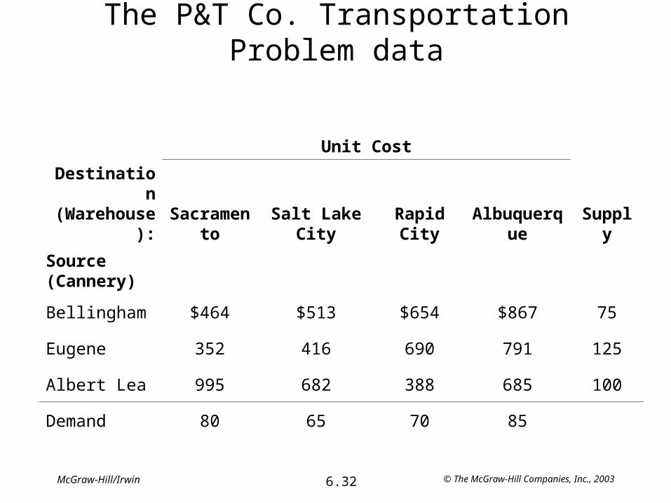
© The McGraw-Hill Companies, Inc., 20036.32McGraw-Hill/Irwin
The P&T Co. Transportation Problem data
Unit Cost
Destination(Warehous
e):Sacrame
ntoSalt Lake
CityRapid City
Albuquerque
Supply
Source (Cannery)
Bellingham $464 $513 $654 $867 75
Eugene 352 416 690 791 125
Albert Lea 995 682 388 685 100
Demand 80 65 70 85

© The McGraw-Hill Companies, Inc., 20036.33McGraw-Hill/Irwin
Network Representation
S1
S2
S3
D4
D2
D1
D3
75
125
100
80
65
70
85
Supplies Demands
SourcesDestinations
(Bellingham)
(Eugene)
(Alber t Lea)
(Sacramento)
(Salt Lake City)
(Rapid City)
(Albuquerque)
464513
654867
352 416690
791
995 682
685
388

© The McGraw-Hill Companies, Inc., 20036.34McGraw-Hill/Irwin
The Transportation Problem is an LP
Let xij = the number of truckloads to ship from cannery i to warehouse j(i = 1, 2, 3; j = 1, 2, 3, 4)
Minimize Cost = $464x11 + $513x12 + $654x13 + $867x14 + $352x21 + $416x22 + $690x23 + $791x24 + $995x31 + $682x32 + $388x33 + $685x34
subject to:Cannery 1: x11 + x12 + x13 + x14 = 75Cannery 2: x21 + x22 + x23 + x24 = 125Cannery 3: x31 + x32 + x33 + x34 = 100Warehouse 1: x11 + x21 + x31 = 80Warehouse 2: x12 + x22 + x32 = 65Warehouse 3: x13 + x23 + x33 = 70Warehouse 4: x14 + x24 + x34 = 85
andxij ≥ 0 (i = 1, 2, 3; j = 1, 2, 3, 4)
From Cannery 2 to all destinationsFrom Cannery 3 to all destinations
From Cannery 1 to all destinations
All canneries can supply all warehouses

© The McGraw-Hill Companies, Inc., 20036.35McGraw-Hill/Irwin
Spreadsheet Formulation
3456789
1011121314151617
B C D E F G H I JUnit Cost Destination (Warehouse)
Sacramento Salt Lake City Rapid City AlbuquerqueSource Bellingham $464 $513 $654 $867
(Cannery) Eugene $352 $416 $690 $791Albert Lea $995 $682 $388 $685
Shipment Quantity Destination (Warehouse)(Truckloads) Sacramento Salt Lake City Rapid City Albuquerque Total Shipped Supply
Source Bellingham 0 20 0 55 75 = 75(Cannery) Eugene 80 45 0 0 125 = 125
Albert Lea 0 0 70 30 100 = 100Total Received 80 65 70 85
= = = = Total CostDemand 80 65 70 85 $152,535

© The McGraw-Hill Companies, Inc., 20036.36McGraw-Hill/Irwin
Integer Solutions Property
As long as all its supplies and demands have integer
values, any transportation problem with feasible
solutions is guaranteed to have an optimal solution with
integer values for all its decision variables. Therefore, it
is not necessary to add constraints to the model that
restrict these variables to only have integer values.

© The McGraw-Hill Companies, Inc., 20036.37McGraw-Hill/Irwin
Distribution System at Proctor and Gamble
• Proctor and Gamble needed to consolidate and re-design their North American distribution system in the early 1990’s.– 50 product categories– 60 plants– 15 distribution centers– 1000 customer zones
• Solved many transportation problems (one for each product category).
• Goal: find best distribution plan, which plants to keep open, etc.
• Closed many plants and distribution centers, and optimized their product sourcing and distribution location.
• Implemented in 1996. Saved $200 million per year.For more details, see 1997 Jan-Feb Interfaces article, “Blending OR/MS,
Judgement, and GIS: Restructuring P&G’s Supply Chain”, downloadable at www.mhhe.com/hillier2e/articles

© The McGraw-Hill Companies, Inc., 20036.38McGraw-Hill/Irwin
Better Products (Assigning Plants to Products)
The Better Products Company has decided to initiate the product of four new products, using three plants that currently have excess capacity.
Unit Cost
Product: 1 2 3 4
Capacity
Available
Plant
1 $41 $27 $28 $24 75
2 40 29 — 23 75
3 37 30 27 21 45
Required production
20 30 30 40
Question: Which plants should produce which products?
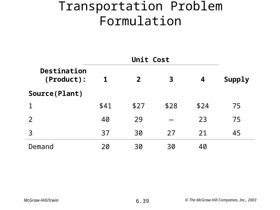
© The McGraw-Hill Companies, Inc., 20036.39McGraw-Hill/Irwin
Transportation Problem Formulation
Unit Cost
Destination (Product): 1 2 3 4 Supply
Source(Plant)
1 $41 $27 $28 $24 75
2 40 29 — 23 75
3 37 30 27 21 45
Demand 20 30 30 40

© The McGraw-Hill Companies, Inc., 20036.40McGraw-Hill/Irwin
Spreadsheet Formulation
3456789
10111213141516
B C D E F G H IUnit Cost Product 1 Product 2 Product 3 Product 4
Plant 1 $41 $27 $28 $24Plant 2 $40 $29 - $23Plant 3 $37 $30 $27 $21
ProducedDaily Production Product 1 Product 2 Product 3 Product 4 At Plant Capacity
Plant 1 0 30 30 0 60 <= 75Plant 2 0 0 0 15 15 <= 75Plant 3 20 0 0 25 45 <= 45
Products Produced 20 30 30 40= = = = Total Cost
Required Production 20 30 30 40 $3,260

© The McGraw-Hill Companies, Inc., 20036.41McGraw-Hill/Irwin
Nifty Co. (Choosing Customers)
• The Nifty Company specializes in the production of a single product, which it produces in three plants.
• Four customers would like to make major purchases. There will be enough to meet their minimum purchase requirements, but not all of their requested purchases.
• Due largely to variations in shipping cost, the net profit per unit sold varies depending on which plant supplies which customer.
Question: How many units should Nifty sell to each customer and how many units should they
ship from each plant to each customer?

© The McGraw-Hill Companies, Inc., 20036.42McGraw-Hill/Irwin
Data for the Nifty Company
Unit Cost
Product: 1 2 3 4
Capacity
Available
Plant
1 $41 $27 $28 $24 75
2 40 29 — 23 75
3 37 30 27 21 45
Required production
20 30 30 40
Question: How many units should Nifty sell to each customer and how many units should
they ship from each plant to each customer?

© The McGraw-Hill Companies, Inc., 20036.43McGraw-Hill/Irwin
Spreadsheet Formulation
3456789
10111213141516171819
B C D E F G H IUnit Profit Customer 1 Customer 2 Customer 3 Customer 4
Plant 1 $55 $42 $46 $53Plant 2 $37 $18 $32 $48Plant 3 $29 $59 $51 $35
Total ProductionShipment Customer 1 Customer 2 Customer 3 Customer 4 Production Quantity
Plant 1 7,000 0 1,000 0 8,000 = 8,000Plant 2 0 0 0 5,000 5,000 = 5,000Plant 3 0 6,000 1,000 0 7,000 = 7,000
Min Purchase 7,000 3,000 2,000 0<= <= <= <= Total Profit
Total Shipped 7,000 6,000 2,000 5,000 $1,076,000<= <= <= <=
Max Purchase 7,000 9,000 6,000 8,000

© The McGraw-Hill Companies, Inc., 20036.44McGraw-Hill/Irwin
Metro Water (Distributing Natural Resources)
Metro Water District is an agency that administers water distribution in a large geographic region. The region is arid, so water must be brought in from outside the region.
– Sources of imported water: Colombo, Sacron, and Calorie rivers.– Main customers: Cities of Berdoo, Los Devils, San Go, and Hollyglass.
Cost per Acre Foot
BerdooLos
DevilsSan Go
Hollyglass
Available
Colombo River $160 $130 $220 $170 5
Sacron River 140 130 190 150 6
Calorie River 190 200 230 — 5
Needed 2 5 4 1.5(million
acre feet)Question: How much water should Metro take from each river,
and how much should they send from each river to each city?

© The McGraw-Hill Companies, Inc., 20036.45McGraw-Hill/Irwin
Spreadsheet Formulation
3456789
1011121314151617
B C D E F G H IUnit Cost ($millions) Berdoo Los Devils San Go Hollyglass
Colombo River 160 130 220 170Sacron River 140 130 190 150Calorie River 190 200 230 -
Water Distribution Total(million acre-feet) Berdoo Los Devils San Go Hollyglass From River Available
Colombo River 0 5 0 0 5 <= 5Sacron River 2 0 2.5 1.5 6 <= 6Calorie River 0 0 1.5 0 1.5 <= 5Total To City 2 5 4 1.5
= = = = Total CostNeeded 2 5 4 1.5 ($million)
1,975

© The McGraw-Hill Companies, Inc., 20036.46McGraw-Hill/Irwin
Northern Airplane (Production Scheduling)
Northern Airplane Company produces commercial airplanes. The last stage in production is to produce the jet engines and install them.
– The company must meet the delivery deadline indicated in column 2.– Production and storage costs vary from month to month.
Maximum Production
Unit Cost of Production ($million)
Unit Costof Storage($thousan
d)Month
ScheduledInstallatio
ns
Regular
TimeOvertim
e
Regular
TimeOvertim
e
1 10 20 10 1.08 1.10 15
2 15 30 15 1.11 1.12 15
3 25 25 10 1.10 1.11 15
4 20 5 10 1.13 1.15Question: How many engines should be produced in each of the four months so that the total of the production and storage costs will be
minimized?
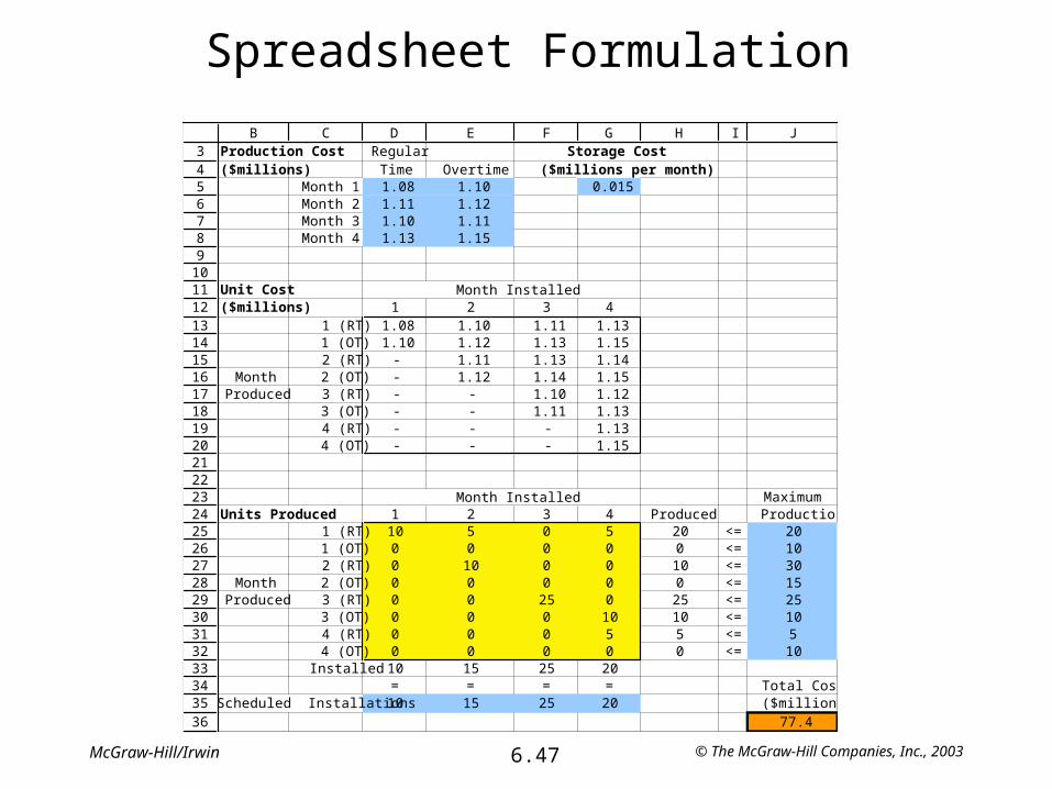
© The McGraw-Hill Companies, Inc., 20036.47McGraw-Hill/Irwin
Spreadsheet Formulation
3456789
101112131415161718192021222324252627282930313233343536
B C D E F G H I JProduction Cost Regular Storage Cost($millions) Time Overtime ($millions per month)
Month 1 1.08 1.10 0.015Month 2 1.11 1.12Month 3 1.10 1.11Month 4 1.13 1.15
Unit Cost($millions) 1 2 3 4
1 (RT) 1.08 1.10 1.11 1.131 (OT) 1.10 1.12 1.13 1.152 (RT) - 1.11 1.13 1.14
Month 2 (OT) - 1.12 1.14 1.15Produced 3 (RT) - - 1.10 1.12
3 (OT) - - 1.11 1.134 (RT) - - - 1.134 (OT) - - - 1.15
MaximumUnits Produced 1 2 3 4 Produced Production
1 (RT) 10 5 0 5 20 <= 201 (OT) 0 0 0 0 0 <= 102 (RT) 0 10 0 0 10 <= 30
Month 2 (OT) 0 0 0 0 0 <= 15Produced 3 (RT) 0 0 25 0 25 <= 25
3 (OT) 0 0 0 10 10 <= 104 (RT) 0 0 0 5 5 <= 54 (OT) 0 0 0 0 0 <= 10
Installed 10 15 25 20= = = = Total Cost
Scheduled Installations 10 15 25 20 ($millions)77.4
Month Installed
Month Installed

© The McGraw-Hill Companies, Inc., 20036.48McGraw-Hill/Irwin
Optimal Production at Northern Airplane
Month
1 (RT)
2 (RT)
3 (RT)
3 (OT)
4 (RT)
Production
20
10
25
10
5
Installations
10
15
25
0
20
Stored
10
5
5
10
0

© The McGraw-Hill Companies, Inc., 20036.49McGraw-Hill/Irwin
Middletown School District
• Middletown School District is opening a third high school and thus needs to redraw the boundaries for the area of the city that will be assigned to the respective schools.
• The city has been divided into 9 tracts with approximately equal populations.
• Each school has a minimum and maximum number of students that should be assigned.
• The school district management has decided that the appropriate objective is to minimize the average distance that students must travel to school.
Question: How many students from each tract should be assigned to each school?

© The McGraw-Hill Companies, Inc., 20036.50McGraw-Hill/Irwin
Data for the Middletown School District
Distance (Miles) to School
Tract 1 2 3Number of High School Students
1 2.2 1.9 2.5 500
2 1.4 1.3 1.7 400
3 0.5 1.8 1.1 450
4 1.2 0.3 2.0 400
5 0.9 0.7 1.0 500
6 1.1 1.6 0.6 450
7 2.7 0.7 1.5 450
8 1.8 1.2 0.8 400
9 1.5 1.7 0.7 500
Minimum enrollment
1,200 1,100 1,000
Maximum enrollment
1,800 1,700 1,500

© The McGraw-Hill Companies, Inc., 20036.51McGraw-Hill/Irwin
Spreadsheet Formulation
3456789
10111213141516171819202122232425262728293031
B C D E F G HDistance (Miles) School 1 School 2 School 3
Tract 1 2.2 1.9 2.5Tract 2 1.4 1.3 1.7Tract 3 0.5 1.8 1.1Tract 4 1.2 0.3 2Tract 5 0.9 0.7 1Tract 6 1.1 1.6 0.6Tract 7 2.7 0.7 1.5Tract 8 1.8 1.2 0.8Tract 9 1.5 1.7 0.7
Number of Total TotalStudents School 1 School 2 School 3 From Tract In Tract
Tract 1 0 500 0 500 = 500Tract 2 400 0 0 400 = 400Tract 3 450 0 0 450 = 450Tract 4 0 400 0 400 = 400Tract 5 350 150 0 500 = 500Tract 6 0 0 450 450 = 450Tract 7 0 450 0 450 = 450Tract 8 0 0 400 400 = 400Tract 9 0 0 500 500 = 500
Min Enrollment 1,200 1,500 1,350<= <= <= Total Distance
Total At School 1,200 1,500 1,350 (miles)<= <= <= 3,530
Max Enrollment 1,800 1,700 1,500

© The McGraw-Hill Companies, Inc., 20036.52McGraw-Hill/Irwin
Energetic (Meeting Energy Needs)
• The Energetic Company needs to make plans for the energy systems for a new building.
• The energy needs fall into three categories:– electricity (20 units)– heating water (10 units)– heating space (30 units)
• The three possible sources of energy are– electricity– natural gas– solar heating unit (limited to 30 units because of roof size)
Question: How should Energetic meet the energy needs for the new building?

© The McGraw-Hill Companies, Inc., 20036.53McGraw-Hill/Irwin
Cost Data for Energetic
Unit Cost
Energy Need: Electricity Water Heating Space Heating
Source of Energy
Electricity $400 $500 $600
Natural gas — 600 500
Solar heater — 300 400

© The McGraw-Hill Companies, Inc., 20036.54McGraw-Hill/Irwin
Spreadsheet Formulation
3456789
101112131415161718
B C D E F G H IEnergy Need
Unit Cost ($/day) Electricity Water Heating Space HeatingSource Electricity 400 500 600
of Natural Gas - 600 500Energy Solar Heater - 300 400
Energy Need TotalDaily Energy Use Electricity Water Heating Space Heating Used
Source Electricity 20 0 0 20of Natural Gas 0 0 10 10 Max Solar
Energy Solar Heater 0 10 20 30 <= 30Total Supplied 20 10 30
= = = Total CostDemand 20 10 30 ($/day)
24,000

© The McGraw-Hill Companies, Inc., 20036.55McGraw-Hill/Irwin
Location of Texago’s Facilities
Type of Facility Locations
Oil fields 1. Several in Texas2. Several in California3. Several in Alaska
Refineries 1. Near New Orleans, Louisiana2. Near Charleston, South Carolina3. Near Seattle, Washington
Distribution Centers 1. Pittsburgh, Pennsylvania2. Atlanta, Georgia3. Kansas City, Missouri4. San Francisco, California

© The McGraw-Hill Companies, Inc., 20036.56McGraw-Hill/Irwin
Potential Sites for Texago’s New Refinery
Potential Site Main Advantages
Near Los Angeles, California
1. Near California oil fields.2. Ready access from Alaska oil fields.3. Fairly near San Francisco distribution center.
Near Galveston, Texas 1. Near Texas oil fields.2. Ready access from Middle East imports.3. Near corporate headquarters.
Near St. Louis, Missouri 1. Low operating costs.2. Centrally located for distribution centers.3. Ready access to crude oil via the Mississippi River.

© The McGraw-Hill Companies, Inc., 20036.57McGraw-Hill/Irwin
Production Data for Texago
Refinery
Crude OilNeeded Annually(Million Barrels) Oil Fields
Crude Oil Produced Annually(Million Barrels)
New Orleans
100 Texas 80
Charleston 60 California 60
Seattle 80 Alaska 100
New site 120 Total 240
Total 360 Needed imports = 360 – 240 = 120
© The McGraw-Hill Companies, Inc., 20036.58McGraw-Hill/Irwin
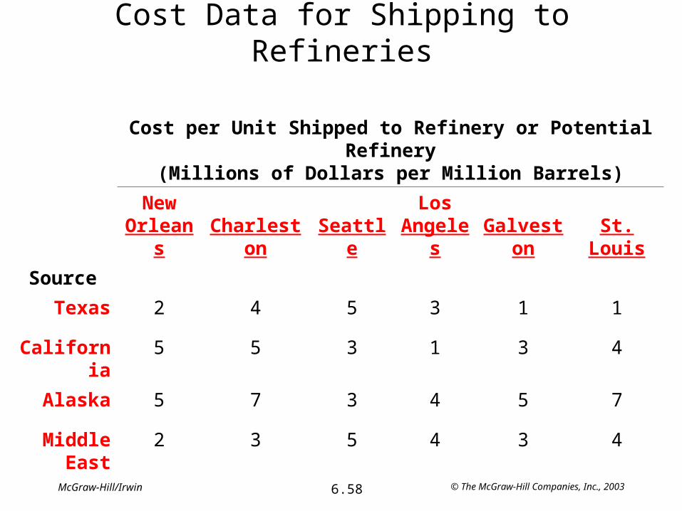
Cost Data for Shipping to Refineries
Cost per Unit Shipped to Refinery or Potential Refinery
(Millions of Dollars per Million Barrels)
New Orlea
nsCharlest
onSeattl
e
Los Angel
esGalves
tonSt.
Louis
Source
Texas 2 4 5 3 1 1
California
5 5 3 1 3 4
Alaska 5 7 3 4 5 7
Middle East
2 3 5 4 3 4

© The McGraw-Hill Companies, Inc., 20036.59McGraw-Hill/Irwin
Cost Data for Shipping to Distribution Centers
Cost per Unit Shipped to Distribution Center
(Millions of Dollars)
Pittsburgh Atlanta
Kansas City
San Francisco
Refinery
New Orleans 6.5 5.5 6 8
Charleston 7 5 4 7
Seattle 7 8 4 3
Potential Refinery
Los Angeles 8 6 3 2
Galveston 5 4 3 6
St. Louis 4 3 1 5
Number of units needed
100 80 80 100

© The McGraw-Hill Companies, Inc., 20036.60McGraw-Hill/Irwin
Estimated Operating Costs for Refineries
Site Annual Operating Cost
(Millions of Dollars)
Los Angeles
Galveston
St. Louis
620
570
530

© The McGraw-Hill Companies, Inc., 20036.61McGraw-Hill/Irwin
Basic Spreadsheet for Shipping to Refineries
3456789
1011121314151617181920
B C D E F G H I JRefineries
Unit Cost ($millions) New Orleans Charleston Seattle New SiteTexas 2 4 5
Oil California 5 5 3Fields Alaska 5 7 3
Middle East 2 3 5
Shipment Quantity Refineries(millions of barrels) New Orleans Charleston Seattle New Site Total Shipped Supply
Texas 0 0 0 0 0 = 80Oil California 0 0 0 0 0 = 60
Fields Alaska 0 0 0 0 0 = 100Middle East 0 0 0 0 0 = 120
Total Received 0 0 0 0= = = = Total Cost
Demand 100 60 80 120 ($millions)0

© The McGraw-Hill Companies, Inc., 20036.62McGraw-Hill/Irwin
Shipping to Refineries, Including Los Angeles
3456789
1011121314151617181920
B C D E F G H I JRefineries
Unit Cost ($millions) New Orleans Charleston Seattle Los AngelesTexas 2 4 5 3
Oil California 5 5 3 1Fields Alaska 5 7 3 4
Middle East 2 3 5 4
Shipment Quantity Refineries(millions of barrels) New Orleans Charleston Seattle Los Angeles Total Shipped Supply
Texas 40 0 0 40 80 = 80Oil California 0 0 0 60 60 = 60
Fields Alaska 0 0 80 20 100 = 100Middle East 60 60 0 0 120 = 120
Total Received 100 60 80 120= = = = Total Cost
Demand 100 60 80 120 ($millions)880

© The McGraw-Hill Companies, Inc., 20036.63McGraw-Hill/Irwin
Shipping to Refineries, Including Galveston
3456789
1011121314151617181920
B C D E F G H I JRefineries
Unit Cost ($millions) New Orleans Charleston Seattle GalvestonTexas 2 4 5 1
Oil California 5 5 3 3Fields Alaska 5 7 3 5
Middle East 2 3 5 3
Shipment Quantity Refineries(millions of barrels) New Orleans Charleston Seattle Galveston Total Shipped Supply
Texas 20 0 0 60 80 = 80Oil California 0 0 0 60 60 = 60
Fields Alaska 20 0 80 0 100 = 100Middle East 60 60 0 0 120 = 120
Total Received 100 60 80 120= = = = Total Cost
Demand 100 60 80 120 ($millions)920

© The McGraw-Hill Companies, Inc., 20036.64McGraw-Hill/Irwin
Shipping to Refineries, Including St. Louis
3456789
1011121314151617181920
B C D E F G H I JRefineries
Unit Cost ($millions) New Orleans Charleston Seattle St. LouisTexas 2 4 5 1
Oil California 5 5 3 4Fields Alaska 5 7 3 7
Middle East 2 3 5 4
Shipment Quantity Refineries(millions of barrels) New Orleans Charleston Seattle St. Louis Total Shipped Supply
Texas 0 0 0 80 80 = 80Oil California 0 20 0 40 60 = 60
Fields Alaska 20 0 80 0 100 = 100Middle East 80 40 0 0 120 = 120
Total Received 100 60 80 120= = = = Total Cost
Demand 100 60 80 120 ($millions)960

© The McGraw-Hill Companies, Inc., 20036.65McGraw-Hill/Irwin
Basic Spreadsheet for Shipping to D.C.’s
3456789
1011121314151617181920
B C D E F G H I JDistribution Center
Unit Cost ($millions) Pittsburgh Atlanta Kansas City San FranciscoNew Orleans 6.5 5.5 6 8
Refineries Charleston 7 5 4 7Seattle 7 8 4 3
New Site
Shipment Quantity Distribution Center(millions of barrels) Pittsburgh Atlanta Kansas City San Francisco Total Shipped Supply
New Orleans 0 0 0 0 0 = 100Refineries Charleston 0 0 0 0 0 = 60
Seattle 0 0 0 0 0 = 80New Site 0 0 0 0 0 = 120
Total Received 0 0 0 0= = = = Total Cost
Demand 100 80 80 100 ($millions)0

© The McGraw-Hill Companies, Inc., 20036.66McGraw-Hill/Irwin
Shipping to D.C.’s When Choose Los Angeles
3456789
1011121314151617181920
B C D E F G H I JDistribution Center
Unit Cost ($millions) Pittsburgh Atlanta Kansas City San FranciscoNew Orleans 6.5 5.5 6 8
Refineries Charleston 7 5 4 7Seattle 7 8 4 3
Los Angeles 8 6 3 2
Shipment Quantity Distribution Center(millions of barrels) Pittsburgh Atlanta Kansas City San Francisco Total Shipped Supply
New Orleans 80 20 0 0 100 = 100Refineries Charleston 0 60 0 0 60 = 60
Seattle 20 0 0 60 80 = 80Los Angeles 0 0 80 40 120 = 120
Total Received 100 80 80 100= = = = Total Cost
Demand 100 80 80 100 ($millions)1,570

© The McGraw-Hill Companies, Inc., 20036.67McGraw-Hill/Irwin
Shipping to D.C.’s When Choose Galveston
3456789
1011121314151617181920
B C D E F G H I JDistribution Center
Unit Cost ($millions) Pittsburgh Atlanta Kansas City San FranciscoNew Orleans 6.5 5.5 6 8
Refineries Charleston 7 5 4 7Seattle 7 8 4 3
Galveston 5 4 3 6
Shipment Quantity Distribution Center(millions of barrels) Pittsburgh Atlanta Kansas City San Francisco Total Shipped Supply
New Orleans 100 0 0 0 100 = 100Refineries Charleston 0 60 0 0 60 = 60
Seattle 0 0 0 80 80 = 80Galveston 0 20 80 20 120 = 120
Total Received 100 80 80 100= = = = Total Cost
Demand 100 80 80 100 ($millions)1,630

© The McGraw-Hill Companies, Inc., 20036.68McGraw-Hill/Irwin
Shipping to D.C.’s When Choose St. Louis
3456789
1011121314151617181920
B C D E F G H I JDistribution Center
Unit Cost ($millions) Pittsburgh Atlanta Kansas City San FranciscoNew Orleans 6.5 5.5 6 8
Refineries Charleston 7 5 4 7Seattle 7 8 4 3
St. Louis 4 3 1 5
Shipment Quantity Distribution Center(millions of barrels) Pittsburgh Atlanta Kansas City San Francisco Total Shipped Supply
New Orleans 100 0 0 0 100 = 100Refineries Charleston 0 60 0 0 60 = 60
Seattle 0 0 0 80 80 = 80St. Louis 0 20 80 20 120 = 120
Total Received 100 80 80 100= = = = Total Cost
Demand 100 80 80 100 ($millions)1,430

© The McGraw-Hill Companies, Inc., 20036.69McGraw-Hill/Irwin
Annual Variable Costs
Site
Total Costof
ShippingCrude Oil
Total Costof Shipping
Finished Product
Operating Cost
for NewRefinery
TotalVariable
Cost
Los Angeles $880 million $1.57 billion $620 million$3.07 billion
Galveston 920 million 1.63 billion 570 million 3.12 billion
St. Louis 960 million 1.43 billion 530 million 2.92 billion

© The McGraw-Hill Companies, Inc., 20036.70McGraw-Hill/Irwin
Sellmore Company Assignment Problem
• The marketing manager of Sellmore Company will be holding the company’s annual sales conference soon.
• He is hiring four temporary employees:– Ann– Ian– Joan– Sean
• Each will handle one of the following four tasks:– Word processing of written presentations– Computer graphics for both oral and written presentations– Preparation of conference packets, including copying and organizing materials– Handling of advance and on-site registration for the conference
Question: Which person should be assigned to which task?
© The McGraw-Hill Companies, Inc., 20036.71McGraw-Hill/Irwin
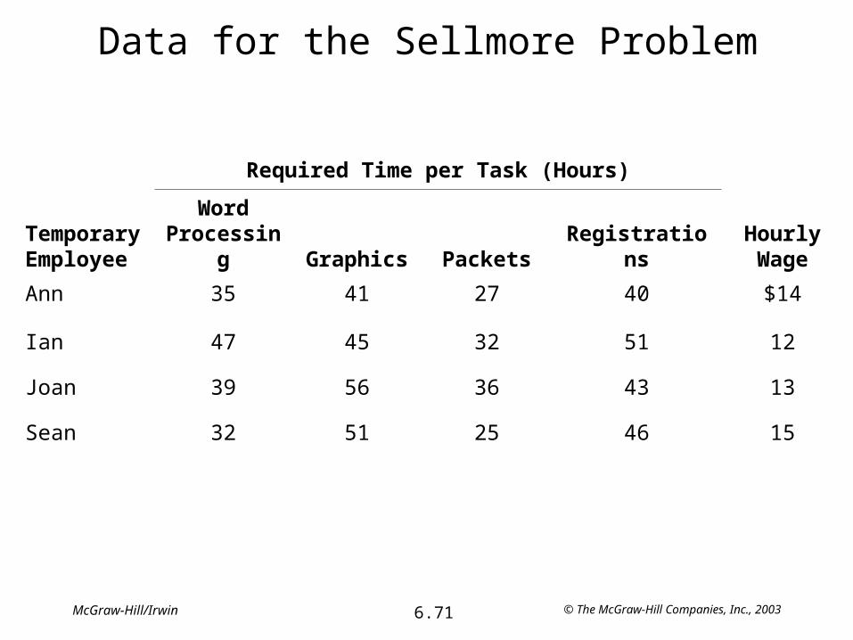
Data for the Sellmore Problem
Required Time per Task (Hours)
TemporaryEmployee
WordProcessin
g Graphics PacketsRegistration
sHourlyWage
Ann 35 41 27 40 $14
Ian 47 45 32 51 12
Joan 39 56 36 43 13
Sean 32 51 25 46 15

© The McGraw-Hill Companies, Inc., 20036.72McGraw-Hill/Irwin
Spreadsheet Formulation
3456789
101112131415161718192021222324252627282930
B C D E F G H I J
Required Time Word Hourly(Hours) Processing Graphics Packets Registrations Wage
Ann 35 41 27 40 $14Assignee Ian 47 45 32 51 $12
Joan 39 56 36 43 $13Sean 32 51 25 46 $15
WordCost Processing Graphics Packets Registrations
Ann $490 $574 $378 $560Assignee Ian $564 $540 $384 $612
Joan $507 $728 $468 $559Sean $480 $765 $375 $690
Word TotalAssignment Processing Graphics Packets Registrations Assignments Supply
Ann 0 0 1 0 1 = 1Assignee Ian 0 1 0 0 1 = 1
Joan 0 0 0 1 1 = 1Sean 1 0 0 0 1 = 1
Total Assigned 1 1 1 1= = = = Total Cost
Demand 1 1 1 1 $1,957
Task
Task
Task

© The McGraw-Hill Companies, Inc., 20036.73McGraw-Hill/Irwin
The Model for Assignment Problems
Given a set of tasks to be performed and a set of assignees who are available to perform these tasks, the problem is to determine which assignee should be assigned to each task.
To fit the model for an assignment problem, the following assumptions need to be satisfied:
1. The number of assignees and the number of tasks are the same.
2. Each assignee is to be assigned to exactly one task.
3. Each task is to be performed by exactly one assignee.
4. There is a cost associated with each combination of an assignee performing a task.
5. The objective is to determine how all the assignments should be made to minimize the total cost.

© The McGraw-Hill Companies, Inc., 20036.74McGraw-Hill/Irwin
The Network Representation
A2
A1
T4A4
T3A3
T2
T1
Assignees Tasks
490
540
468
690
(Ann)
(I an)
(Joan)
(Sean)
(Word processing)
(Graphics)
(Packets)
(Registrations)
574
378560
564
384612
507 728
559
480
765
375

© The McGraw-Hill Companies, Inc., 20036.75McGraw-Hill/Irwin
Job Shop (Assigning Machines to Locations)
• The Job Shop Company has purchased three new machines of different types.
• There are five available locations where the machine could be installed.
• Some of these locations are more desirable for particular machines because of their proximity to work centers that will have a heavy work flow to these machines.
Question: How should the machines be assigned to locations?

© The McGraw-Hill Companies, Inc., 20036.76McGraw-Hill/Irwin
Materials-Handling Cost Data
Cost per Hour
Location: 1 2 3 4 5
Machine
1 $13 $16 $12 $14 $15
2 15 — 13 20 16
3 4 7 10 6 7

© The McGraw-Hill Companies, Inc., 20036.77McGraw-Hill/Irwin
Spreadsheet Formulation
3456789
1011121314151617
B C D E F G H I JCost ($/hour) Location 1 Location 2 Location 3 Location 4 Location 5
Machine 1 13 16 12 14 15Machine 2 15 - 13 20 16Machine 3 4 7 10 6 7
TotalAssignment Location 1 Location 2 Location 3 Location 4 Location 5 Assignments Supply
Machine 1 0 0 0 1 0 1 = 1Machine 2 0 0 1 0 0 1 = 1Machine 3 1 0 0 0 0 1 = 1
Total Assigned 1 0 1 1 0<= <= <= <= <= Total Cost
Demand 1 1 1 1 1 ($/hour)31

© The McGraw-Hill Companies, Inc., 20036.78McGraw-Hill/Irwin
Better Products (No Product Splitting)
3456789
101112131415161718192021222324
B C D E F G H IUnit Cost Product 1 Product 2 Product 3 Product 4
Plant 1 $41 $27 $28 $24Plant 2 $40 $29 - $23Plant 3 $37 $30 $27 $21
Required Production 20 30 30 40
Cost ($/day) Product 1 Product 2 Product 3 Product 4Plant 1 $820 $810 $840 $960Plant 2 $800 $870 - $920Plant 3 $740 $900 $810 $840
TotalAssignment Product 1 Product 2 Product 3 Product 4 Assignments Supply
Plant 1 0 1 1 0 2 <= 2Plant 2 1 0 0 0 1 <= 2Plant 3 0 0 0 1 1 = 1
Total Assigned 1 1 1 1= = = = Total Cost
Demand 1 1 1 1 $3,290

© The McGraw-Hill Companies, Inc., 20036.79McGraw-Hill/Irwin
Middletown School District (No Tract Splitting)
3456789
101112131415161718192021222324252627282930
B C D E F G H I J KDistance Number of Cost(Miles) School 1 School 2 School 3 Students (Miles) School 1 School 2 School 3
Tract 1 2.2 1.9 2.5 500 Tract 1 1100 950 1250Tract 2 1.4 1.3 1.7 400 Tract 2 560 520 680Tract 3 0.5 1.8 1.1 450 Tract 3 225 810 495Tract 4 1.2 0.3 2 400 Tract 4 480 120 800Tract 5 0.9 0.7 1 500 Tract 5 450 350 500Tract 6 1.1 1.6 0.6 450 Tract 6 495 720 270Tract 7 2.7 0.7 1.5 450 Tract 7 1215 315 675Tract 8 1.8 1.2 0.8 400 Tract 8 720 480 320Tract 9 1.5 1.7 0.7 500 Tract 9 750 850 350
TotalAssignment School 1 School 2 School 3 Assignments Supply
Tract 1 0 1 0 1 = 1Tract 2 1 0 0 1 = 1Tract 3 1 0 0 1 = 1Tract 4 0 1 0 1 = 1Tract 5 1 0 0 1 = 1Tract 6 0 0 1 1 = 1Tract 7 0 1 0 1 = 1Tract 8 0 0 1 1 = 1Tract 9 0 0 1 1 = 1
Total Assigned 3 3 3= = = Total Distance
Demand 3 3 3 (Miles)3560
© The McGraw-Hill Companies, Inc., 20036.80McGraw-Hill/Irwin
The Transportation Problem
• A common problem in logistics is how to transport goods from a set of sources (e.g., plants, warehouses, etc.) to a set of destinations (e.g., warehouses, customers, etc.) at the minimum possible cost.
• Given– a set of sources, each with a given supply,– a set of destinations, each with a given demand,– a cost table (cost/unit to ship from each source to each destination)
• Goal– Choose shipping quantities from each source to each destination so as to
minimize total shipping cost.

© The McGraw-Hill Companies, Inc., 20036.81McGraw-Hill/Irwin
The Network Representation
Sources Destinations
Supply1
Supply2
Supply3
Demand1
Demand2
Demand3
Demand4CostijShipment Quantityij

© The McGraw-Hill Companies, Inc., 20036.82McGraw-Hill/Irwin
Transportation Problem ExampleA company has two plants (in Seattle and Atlanta) producing a certain product that is to be shipped to three distribution centers (in Sacramento, St. Louis, and Pittsburgh).
– The unit production costs are the same at the two plants, and the shipping costs per unit are shown in the table below.
– Shipments are made once per week.– During each week, each plant produces at most 60 units and each distribution center needs
at least 40 units.Unit Shipping Cost
Distribution Center
Sacramento
St. LouisPittsbur
gh
PlantSeattle $2 $6 $8
Atlanta $7 $5 $3Question: How many units should be shipped from
each plant to each distribution center?

© The McGraw-Hill Companies, Inc., 20036.83McGraw-Hill/Irwin
Spreadsheet Solution
3
45678
9
101112131415
B C D E F G HSacramento St. Louis Pittsburgh
Cost Dist. Center Dist. Center Dist. CenterSeattle Plant $2 $6 $8Atlanta Plant $7 $5 $3
Shipment Sacramento St. Louis Pittsburgh
Quantities Dist. Center Dist. Center Dist. Center Shipped AvailableSeattle Plant 40 20 0 60 <= 60Atlanta Plant 0 20 40 60 <= 60
Shipped 40 40 40 Cost = $420>= >= >=
Needed 40 40 40

© The McGraw-Hill Companies, Inc., 20036.84McGraw-Hill/Irwin
Shipping from D.C.’s to Customers
The same company ships one of its products from its three distribution centers to four different customers
– The shipping costs per unit are shown in the table below.– Shipments are made once per week.– During each week, each distribution center has received 40 units.– Customer demand is also shown in the table below.
Unit Shipping Cost
Customer
1 2 3 4
Distribution
Center
Sacramento
$8 $10 $7 $11
St. Louis $12 $11 $9 $6
Pittsburgh $10 $9 $15 $10
Customer Demand 40 30 25 25Question: How many units should be shipped from each distribution center to each customer?
© The McGraw-Hill Companies, Inc., 20036.85McGraw-Hill/Irwin
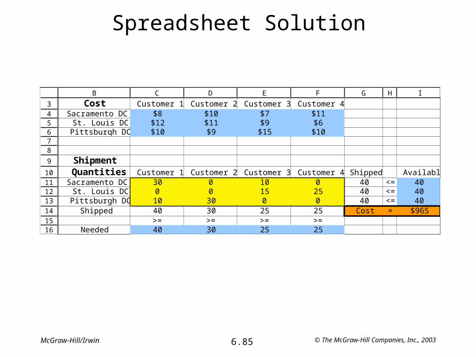
Spreadsheet Solution
345678
9
10111213141516
B C D E F G H I
Cost Customer 1 Customer 2 Customer 3 Customer 4Sacramento DC $8 $10 $7 $11
St. Louis DC $12 $11 $9 $6Pittsburgh DC $10 $9 $15 $10
ShipmentQuantities Customer 1 Customer 2 Customer 3 Customer 4 Shipped Available
Sacramento DC 30 0 10 0 40 <= 40St. Louis DC 0 0 15 25 40 <= 40
Pittsburgh DC 10 30 0 0 40 <= 40Shipped 40 30 25 25 Cost = $965
>= >= >= >=Needed 40 30 25 25

© The McGraw-Hill Companies, Inc., 20036.86McGraw-Hill/Irwin
Managing the Whole Supply Chain(Plant to D.C. to Customer)
3
45678
9
1011121314151617
1819
202122232425
26
272829303132333435
B C D E F G H ISacramento St. Louis Pittsburgh
Cost Dist. Center Dist. Center Dist. CenterSeattle Plant $2 $6 $8Atlanta Plant $7 $5 $3
Shipment Sacramento St. Louis Pittsburgh
Quantities Dist. Center Dist. Center Dist. Center Shipped AvailableSeattle Plant 60 0 0 60 <= 60Atlanta Plant 0 25 35 60 <= 60
Shipped 60 25 35 Cost = $350
Distribution from DC's to Customers
Cost Customer 1 Customer 2 Customer 3 Customer 4Sacramento DC $8 $10 $7 $11
St. Louis DC $12 $11 $9 $6Pittsburgh DC $10 $9 $15 $10
ShipmentQuantities Customer 1 Customer 2 Customer 3 Customer 4 Shipped Available
Sacramento DC 35 0 25 0 60 <= 60St. Louis DC 0 0 0 25 25 <= 25
Pittsburgh DC 5 30 0 0 35 <= 35Shipped 40 30 25 25 Cost = $925
>= >= >= >=Needed 40 30 25 25
Total Cost = $1,275

© The McGraw-Hill Companies, Inc., 20036.87McGraw-Hill/Irwin
Site Selection
• The lease is up on their distribution center in St. Louis. They now must decide whether to sign a new lease in St. Louis, or move the distribution center to a new location.
• One possible new location is Omaha, Nebraska, which is offering a better deal on the lease.
Question: Should they move their distribution center to Omaha?

© The McGraw-Hill Companies, Inc., 20036.88McGraw-Hill/Irwin
Spreadsheet Solution to Site Selection
123
45678
9
1011121314151617
1819
202122232425
26
272829303132333435
A B C D E F G H I
Distribution from Plants to DC's
Sacramento Omaha PittsburghCost Dist. Center Dist. Center Dist. Center
Seattle Plant $2 $5 $8Atlanta Plant $7 $6 $3
Shipment Sacramento Omaha Pittsburgh
Quantities Dist. Center Dist. Center Dist. Center Shipped AvailableSeattle Plant 60 0 0 60 <= 60Atlanta Plant 0 0 60 60 <= 60
Shipped 60 0 60 Cost = $300
Distribution from DC's to Customers
Cost Customer 1 Customer 2 Customer 3 Customer 4Sacramento DC $8 $10 $7 $11
Omaha DC $13 $10 $8 $8Pittsburgh DC $10 $9 $15 $10
ShipmentQuantities Customer 1 Customer 2 Customer 3 Customer 4 Shipped Available
Sacramento DC 35 0 25 0 60 <= 60Omaha DC 0 0 0 0 0 <= 0
Pittsburgh DC 5 30 0 25 60 <= 60Shipped 40 30 25 25 Cost = $1,025
>= >= >= >=Needed 40 30 25 25
Total Cost = $1,325

© The McGraw-Hill Companies, Inc., 20036.89McGraw-Hill/Irwin
Distribution System at Proctor and Gamble
• Proctor and Gamble needed to consolidate and re-design their North American distribution system in the early 1990’s.
– 50 product categories– 60 plants– 15 distribution centers– 1000 customer zones
• Solved many transportation problems (one for each product category).
• Goal: find best distribution plan, which plants to keep open, etc.
• Closed many plants and distribution centers, and optimized their product sourcing and distribution location.
• Implemented in 1996. Saved $200 million per year.
For more details, see 1997 Jan-Feb Interfaces article, “Blending OR/MS, Judgement, and GIS: Restructuring P&G’s Supply Chain”, downloadable at
www.mhhe.com/hillier2e/articles

© The McGraw-Hill Companies, Inc., 20036.90McGraw-Hill/Irwin
The Assignment Problem
• The job of assigning people (or machines or whatever) to a set of tasks is called an assignment problem.
• Given– a set of assignees– a set of tasks– a cost table (cost associated with each assignee performing each task)
• Goal– Match assignees to tasks so as to perform all of the tasks at the minimum
possible cost.

© The McGraw-Hill Companies, Inc., 20036.91McGraw-Hill/Irwin
Network Representation
Assignees Tasks
Costij

© The McGraw-Hill Companies, Inc., 20036.92McGraw-Hill/Irwin
Assignment Problem Example
The coach of a swim team needs to assign swimmers to a 200-yard medley relay team (four swimmers, each swims 50 yards of one of the four strokes). Since most of the best swimmers are very fast in more than one stroke, it is not clear which swimmer should be assigned to each of the four strokes. The five fastest swimmers and their best times (in seconds) they have achieved in each of the strokes (for 50 yards) are shown below.
Backstroke
Breaststroke
Butterfly Freestyle
Carl 37.7 43.4 33.3 29.2
Chris 32.9 33.1 28.5 26.4
David 33.8 42.2 38.9 29.6
Tony 37.0 34.7 30.4 28.5
Ken 35.4 41.8 33.6 31.1
Question: How should the swimmers be assigned to make the fastest relay team?

© The McGraw-Hill Companies, Inc., 20036.93McGraw-Hill/Irwin
Algebraic Formulation
Let xij = 1 if swimmer i swims stroke j; 0 otherwisetij = best time of swimmer i in stroke j
Minimize Time = ∑ i ∑ j tij xij
subject to:
each stroke swum: ∑ i xij = 1 for each stroke j
each swimmer swims 1: ∑ j xij ≤ 1 for each swimmer i
andxij ≥ 0 for all i and j.

© The McGraw-Hill Companies, Inc., 20036.94McGraw-Hill/Irwin
Spreadsheet Formulation
3456789
10
111213141516171819
B C D E F G H I
Best Times Backstroke Breastroke Butterfly FreestyleCarl 37.7 43.4 33.3 29.2Chris 32.9 33.1 28.5 26.4David 33.8 42.2 38.9 29.6Tony 37.0 34.7 30.4 28.5Ken 35.4 41.8 33.6 31.1
Assignment Backstroke Breastroke Butterfly FreestyleCarl 0 0 0 1 1 <= 1Chris 0 0 1 0 1 <= 1David 1 0 0 0 1 <= 1Tony 0 1 0 0 1 <= 1Ken 0 0 0 0 0 <= 1
1 1 1 1 Time = 126.2= = = =1 1 1 1

© The McGraw-Hill Companies, Inc., 20036.95McGraw-Hill/Irwin
Bidding for Classes
• In the MBA program at a prestigious university in the Pacific Northwest, students bid for electives in the second year of their program.
• Each of the 10 students has 100 points to bid (total) and must take two electives.
• There are four electives available:– Quantitative Methods– Finance– Operations Management– Accounting
• Each class is limited to 5 students.
Question: How should students be assigned to the classes?

© The McGraw-Hill Companies, Inc., 20036.96McGraw-Hill/Irwin
Points Bid for Electives
Electives
Student
Quantitative
Methods Finance
OperationsManageme
nt Accounting
George 60 10 10 20
Fred 20 20 40 20
Ann 45 45 5 5
Eric 50 20 5 25
Susan 30 30 30 10
Liz 50 50 0 0
Ed 70 20 10 0
David 25 25 35 15
Tony 35 15 35 15
Jennifer 60 10 10 20

© The McGraw-Hill Companies, Inc., 20036.97McGraw-Hill/Irwin
Spreadsheet Solution(Maximizing Total Points)
34567891011121314
15
1617181920212223242526272829
B C D E F G H I J K
Points QMETH Finance Op Mgt. AccountingGeorge 60 10 10 20
Fred 20 20 40 20Ann 45 45 5 5Eric 50 20 5 25
Susan 30 30 30 10Liz 50 50 0 0Ed 70 20 10 0
David 25 25 35 15Tony 35 15 35 15
Jennifer 60 10 10 20
Total Classes StudentAssignment QMETH Finance Op Mgt. Accounting Classes to Take Points
George 1 0 0 1 2 = 2 80Fred 0 0 1 1 2 = 2 60Ann 1 1 0 0 2 = 2 90Eric 0 1 0 1 2 = 2 45
Susan 0 1 1 0 2 = 2 60Liz 1 1 0 0 2 = 2 100Ed 1 0 1 0 2 = 2 80
David 0 1 1 0 2 = 2 60Tony 0 0 1 1 2 = 2 50
Jennifer 1 0 0 1 2 = 2 805 5 5 5
<= <= <= <= Total Points = 705Capacity 5 5 5 5

© The McGraw-Hill Companies, Inc., 20036.98McGraw-Hill/Irwin
Spreadsheet Solution(Maximizing the Minimum Student Point
Total)
34567891011121314
15
161718192021222324252627282930
B C D E F G H I J K L M
Points QMETH Finance Op Mgt. AccountingGeorge 60 10 10 20
Fred 20 20 40 20Ann 45 45 5 5Eric 50 20 5 25
Susan 30 30 30 10Liz 50 50 0 0Ed 70 20 10 0
David 25 25 35 15Tony 35 15 35 15
Jennifer 60 10 10 20
Total Classes MinAssignment QMETH Finance Op Mgt. Accounting Classes to Take Points Points
George 1 0 0 1 2 = 2 80 >= 50Fred 0 1 1 0 2 = 2 60 >= 50Ann 0 1 0 1 2 = 2 50 >= 50Eric 1 0 1 0 2 = 2 55 >= 50
Susan 0 1 1 0 2 = 2 60 >= 50Liz 0 1 0 1 2 = 2 50 >= 50Ed 1 0 0 1 2 = 2 70 >= 50
David 0 1 1 0 2 = 2 60 >= 50Tony 1 0 1 0 2 = 2 70 >= 50
Jennifer 1 0 0 1 2 = 2 80 >= 505 5 5 5
<= <= <= <= Total Points = 635Capacity 5 5 5 5
Min Points = 50