me 581: simulation of mechanical system

1 Copyright © 20xx by ASME

ME 581: SIMULATION OF MECHANICAL SYSTEM

KINEMATIC ANALYSIS OF DISPLACMENT AMPLIFING COMPLIANT MECHANISM USING HAUG’S METHOD

Ahmad Emam Graduate Student

Pennsylvania State University

ABSTRACT

Displacement-amplifying compliant mechanisms (DaCMs) reported in literature are widely used for actuator applications (HOWELL, 2001). This paper will do a kinematic analysis on one kind of DaCM with Haug’s method to verify the mechanism output/input displacement ratio.

INTRODUCTION Compliant mechanisms (HOWELL, 2001) are becoming increasingly popular due to their inherent advantages over the traditional rigid-body mechanisms and their amenability to small-sized systems of the rapidly growing areas of micro- and nanosystems (ANANTHASURESH & AND HOWELL, 2005). Displacement-amplifying compliant mechanisms DaCMs are used to get large displacement at the output as compared to that at the input (KRISHNAN & ANANTHASURESH, 2008). In this paper, we will review the mechanical performance of one kind of DaCM with kinematic analysis of Haug’s method. Using Haug’s method we developed a MATLAB code to numericaly simulate the mechanism and estimate the exact output/input displacement ratio.

TOPOLOGY AND MOBILITY DaCM model that we used in this study can be found

online in one of free 3D models library. It claims to have 15:1 input/output displacement ratio.

The topology of the system can be interpreted as in Figure2. This model has 1 DOF of freedom, but because of some technical issues the Jacobian’s of this system will always be singular and that cause a problem with Haug’s method. So, we switched to an alternative interpretation of the model Figure3. It have the same DOF and works great with the method. We replaced all three links 4,5 and 6 with a slider mechanism as it should be represented in the CM designs.

Figure 1 DaCM model for the study

Figure 2 Topology and skeletal diagram of the model


COORDINATES The mechanism has 3 links other than the ground and

hence nine coordinates. The coordinates of the ith link are given as follows.

The origin of local coordinate frames attached to the links

with respect to the global coordinate frame are given by {ri}. the coordinates of a point ‘P’ attatched to link ‘i’ with respect to the global coordinate and local coordinates are given by {ri}P and {si}`P ,respectivly. As in the following relationship.

Where,

Table 1 Estimated global coordinates of the system

Link 1 2 3 4

{ri} xi 0 -22.36 -8 0

yi 0 0 9 27.25

Table 2 Estimated local coordinates of the system

{s1}’ {s2}’ {s3}’ {s4}’ A {-22.63 , 0 } { 0, 0 } B {7.75 , 0 } C {0,0} D {14.88 , 16 } {29.75,7} E {14.88,7} F {0,0}

W {40,-6} Z {0,19.75}

CONSTRAINT VECTOR The mechanism has two revolute, two double revolute and

one prismatic joints hence eight kinematic constraints. Also, one driver constraints must be specified as the system has 1 degree of freedom (DOF).

Where,

and the driver constraints specify the attitude of link 2.

JACOBIAN The Jacobian of the system can be derived using the

following general formulas for each joint. For simple revolute,

Figure 3 Alternative interpretation of the System with local coordinates.


For double revolute,

For slider,

The Jacobian of the system must be a square matrix with

rows and columns equals to the number of the constraints vector. In this system, the Jacobian is 9x9 matrix.

POSITION SOLUTION The position solution of the system may be obtained by

giving an initial guess and then employing Newton-Raphson equation with the constraint vector and the Jacobian to find the position solutions at specific attitude values of link2 (0 to 0.1π).

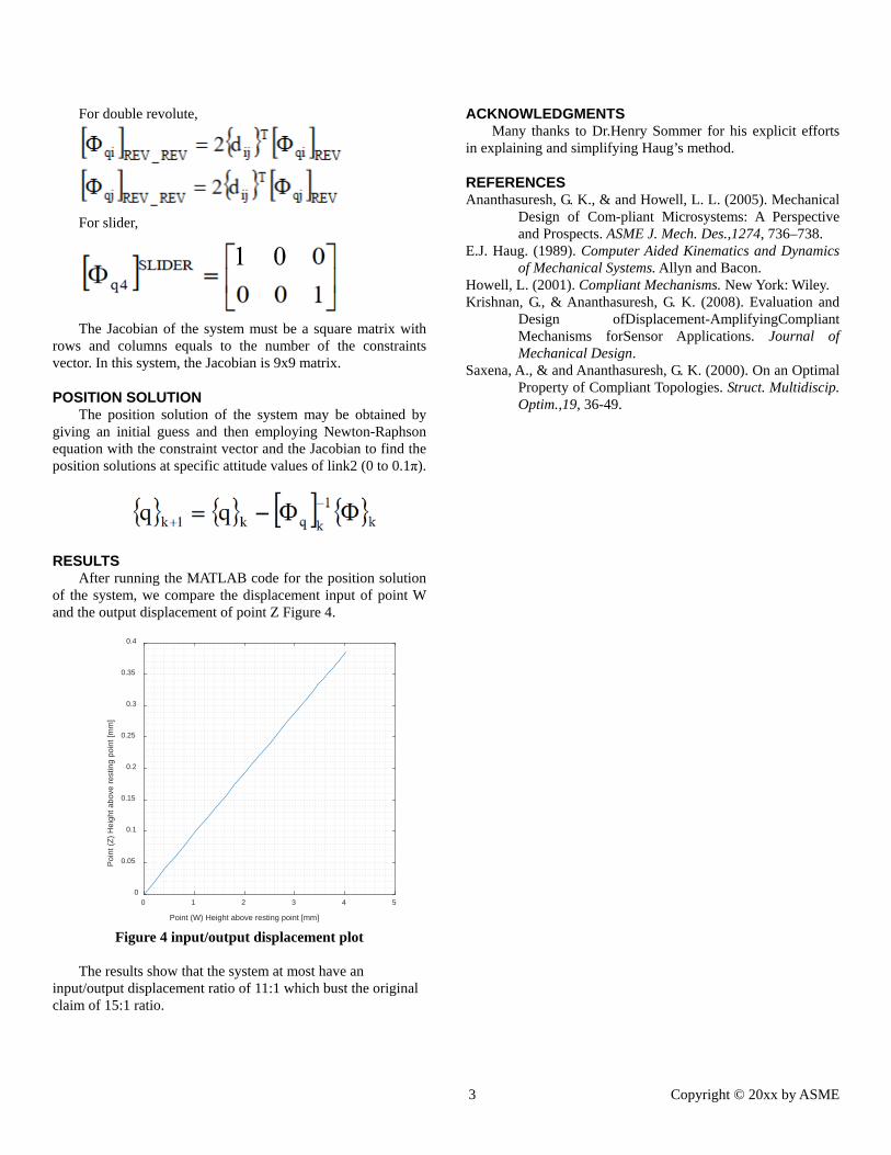
RESULTS After running the MATLAB code for the position solution

of the system, we compare the displacement input of point W and the output displacement of point Z Figure 4.

0 1 2 3 4 5

Point (W) Height above resting point [mm]

0

0.05

0.1

0.15

0.2

0.25

0.3

0.35

0.4

Poin

t (Z)

Hei

ght a

bove

rest

ing

poin

t [m

m]

Figure 4 input/output displacement plot

The results show that the system at most have an

input/output displacement ratio of 11:1 which bust the original claim of 15:1 ratio.

ACKNOWLEDGMENTS Many thanks to Dr.Henry Sommer for his explicit efforts

in explaining and simplifying Haug’s method.

REFERENCES Ananthasuresh, G. K., & and Howell, L. L. (2005). Mechanical

Design of Com-pliant Microsystems: A Perspective and Prospects. ASME J. Mech. Des.,1274, 736–738.

E.J. Haug. (1989). Computer Aided Kinematics and Dynamics of Mechanical Systems. Allyn and Bacon.

Howell, L. (2001). Compliant Mechanisms. New York: Wiley. Krishnan, G., & Ananthasuresh, G. K. (2008). Evaluation and

Design ofDisplacement-AmplifyingCompliant Mechanisms forSensor Applications. Journal of Mechanical Design.

Saxena, A., & and Ananthasuresh, G. K. (2000). On an Optimal Property of Compliant Topologies. Struct. Multidiscip. Optim.,19, 36-49.


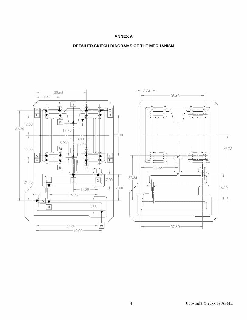
ANNEX A

DETAILED SKITCH DIAGRAMS OF THE MECHANISM


ANNEX B

THE JACOBIAN MATRIX OF THE SYSTEM


ANNEX C

MATLAB CODES

% cm_main_sc.m - compliant mechanism for ME 581 % initialize cm_ini_sc % one crank revolution tpr = pi; % 20 degree freedom dt = tpr / 60; % 180 positions %tpr = 0; % single position % starting position phi2_0 = 0 * d2r; % start at zero % mechanism animation plots s2anim = [0 0 40 40 0; 0 -6 -6 0 0]; s3anim = [0 30 30 -3 -3 0; 0 0 7 7 0 0]; s4anim = [0 12 12 -12 -12 0; 0 0 19 19 0 0]; % timer loop keep = []; keep_q = []; for t = 0 : dt : tpr, phi2_0 = 0.1*sin(t); % kinematics cm_kin_sc; % save kinematics ang2 = phi2 / d2r; ang3 = phi3 / d2r; detJAC = det(JAC); y2W = r2W(2)+6; y4Z = r4Z(2)-46.08; keep = [ keep ; ang2 ang3 detJAC y2W y4Z ]; keep_q = [ keep_q ; q' ]; % mechanism animation drBC = [r2B r3C]; drEF = [r3E r4F]; r2Shape = r2 + A2*s2anim; r3Shape = r3 + A3*s3anim; r4Shape = r4 + A4*s4anim; plot(r2Shape(1,:),r2Shape(2,:)) hold on plot(r3Shape(1,:),r3Shape(2,:)) plot(r4Shape(1,:),r4Shape(2,:)) plot(drBC(1,:),drBC(2,:)) plot(drEF(1,:),drEF(2,:)) plot(0,46.08,'.') axis([-30 30 -10 50],'square') hold off pause(0.1)


end % plot ang2 = keep(:,1); ang3 = keep(:,2); detJAC = keep(:,3); y2W = keep(:,4); y4Z = keep(:,5); Screw = y2W/0.5; figure plot(y2W,y4Z) xlabel('Point (W) Height above resting point [mm]') ylabel('Point (Z) Height above resting point [mm]') axis('square') grid minor figure plot(Screw,y4Z) xlabel('Screw Cycles [0.5 pitch]') ylabel('Point (Z) Height above resting point [mm]') axis('square') grid minor figure plot(y2W,detJAC) xlabel('Screw Cycles [0.5 pitch]') ylabel('Point (Z) Height above resting point [mm]') axis('square') grid minor


% cm_ini_sc.m - compliant mechanism for ME 581 % initialize constants and assembly guesses % general constants d2r = pi / 180; R = [ 0 -1 ; 1 0 ]; % mechanism constants s2pA = [ 0 0 ]'; s2pB = [ 7.75 0 ]'; s2pW = [ 40 -6 ]'; s3pC = [ 0 0 ]'; s3pD = [ 29.75 7 ]'; s3pE = [ 14.88 7 ]'; s4pF = [ 0 0 ]'; s4pZ = [ 0 19.75 ]'; r1A = [ -22.63 0 ]'; r1D = [ 14.88 16 ]'; % double revolute lengths BC = 9; EF = 10.33; % initial guesses phi2 = 0 * d2r; phi3 = 0 * d2r; phi4 = 0 * d2r; q(1,1) = -22.36; q(2,1) = 0; q(3,1) = phi2; q(4,1) = -8; q(5,1) = 9; q(6,1) = phi3; q(7,1) = 0; q(8,1) = 27.25; q(9,1) = phi4; % driver for crank - phi2 = phi2_0 + w2*t phi2_0 = 0 * d2r; w2 = 0; % +60 * 2 * pi / 60; % 60 rpm CCW, convert to rad/sec t = 0; % bottom of cm_ini_sc


% cm_phi_sc.m - compliant mechanism for ME 581 % evaluate constraints and Jacobian for crank driving constraint % global location of local frames and rotation matrices r2 = q(1:2); phi2 = q(3); r3 = q(4:5); phi3 = q(6); r4 = q(7:8); phi4 = q(9); A2 = [ cos(phi2) -sin(phi2); sin(phi2) cos(phi2) ]; A3 = [ cos(phi3) -sin(phi3); sin(phi3) cos(phi3) ]; A4 = [ cos(phi4) -sin(phi4); sin(phi4) cos(phi4) ]; B2 = R * A2; B3 = R * A3; B4 = R * A4; % global locations of points r2A = r2 + A2*s2pA; r2B = r2 + A2*s2pB; r2W = r2 + A2*s2pW; r3C = r3 + A3*s3pC; r3D = r3 + A3*s3pD; r3E = r3 + A3*s3pE; r4F = r4 + A4*s4pF; r4Z = r4 + A4*s4pZ; x4 = r4(1); % double revolute dij = rjP - riP d23BC = r3C - r2B; d34EF = r4F - r3E; % revolute constraints PHI(1:2,1) = r2A - r1A; PHI(3,1) = d23BC'*d23BC-BC^2; PHI(4:5,1) = r3D - r1D; PHI(6,1) = d34EF'*d34EF-EF^2; PHI(7:8,1) = [ x4 phi4 ]'; % crank driver constraint PHI(9,1) = phi2 - phi2_0 - w2*t; % Jacobian by rows JAC = zeros(9,9); % Link2 JAC(1:2,1:3) = [ eye(2) B2*s2pA ]; JAC(3,1:3) = -2*d23BC'*[ eye(2) B2*s2pB ]; % Link3 JAC(3,4:6) = 2*d23BC'*[ eye(2) B3*s3pC ]; JAC(4:5,4:6) = [ eye(2) B3*s3pD ]; JAC(6,4:6) = -2*d34EF'*[ eye(2) B3*s3pE ];


% Link4 JAC(6,7:9) = 2*d34EF'*[ eye(2) B4*s4pF ]; JAC(7,7) = 1; JAC(8,9) = 1; % driver constraint in Jacobian JAC(9,3) = 1; % current results current_crank = phi2 / d2r; % bottom of cm_phi_sc % cm_kin_sc.m - compliant mechanism for ME 581 % positon, velocity, and acceleration % Newton-Raphson position solution assy_tol = 1e-5; cm_phi_sc; while max(abs(PHI)) > assy_tol, q = q - inv(JAC) * PHI; cm_phi_sc; end % bottom of cm_kin_sc

ME 581: Simulation of Mechanical

Systems Kinematic and Dynamic Analysis of an

Excavator Arm

Nicholas Holowsko

Abstract

Excavator(or Track hoe) arms are designed to

transmit high amounts of force for reshaping the

environment around it, and to give the operator a

large degree of movement and accuracy in the

process. This study attempts to piece together the

parts of the arm and their purpose, while analyzing

the motion of the machine as a whole. Here, the

model is based off of a Link-Belt 800LX excavator

model, and all assumptions and measurements are

based off of technical specifications for this vehicle

model. This paper will present a mechanism

overview, a kinematic and dynamic analysis, and a

discussion on model limitations.

2. Methodology

2.1. Initial Conditions

Initial measurements and performance

requirements for this model were based off of a

technical specifications sheet for an excavator

model. Weights and geometry for the main link

arms were taken from here. Figure 1 shows a side

view from the specifications sheet[1].

This excavator, as with most designs, can be

approximated in 2D with 12 Links. 1 link acts as

the ground, 3 are the main arm, the bucket arm, and

the bucket itself, 2 comprise the linkages

connecting the bucket to the bucket arm, and 6 links

make up the 3 hydraulic arms. Additionally, 12

revolute links connect the rigid steel parts of the

arm, and 3 prismatic links connect each of the

hydraulic pistons. Links and joint labels are shown

in figure 2.

Mass and link size was obtained from the

specifications sheet and simplified for the sake of

this project. Results are shown in table 1. Bucket

linkages were not on the spec sheet and mass was

estimated using polygeom.m, areas, and the density

of steel. Bucket linkage mass is doubled in the

model because they typically appear on both sides

of the mechanism. The hydraulic arm mass is split

evenly between both links connecting the prismatic.

The mass of the hydraulic actuator is doubled for

links 7 and 8 as it appears on both sides of the

mechanism.

Description Link Mass(kg)

Main Arm 2 8000

Bucket Arm 3 4000

Bucket Arm 4 3000

Bucket Linkages 5,6 100

Hydraulic Arms 7,8,9,10,11,12 800

Table 1: Initial mass data for the links

Additional information taken from the spec sheet

includes engine output and hydraulic system flow

rate. The engine for this excavator model has a max

output horsepower of 444 HP. This will later be

used to confirm that dynamic results are reasonable.

Hydraulic pump flow was found to total 264.2 gpm.

Divided by 4 hydraulic cylinders with ~8 inch

bores, the hydraulic pistons could extend at 0.13

m/s at max.

Figure 2: Link-Joint model of excavator

Figure 1: Side view of Link-Belt excavator

Polar moments of inertia and link centers of gravity

were found using the polygeom.m Matlab script.

The image shown in figure 1 was digitized and the

outlines and joint locations brought into Matlab.

All local coordinate frames were attached at link

centers of gravity. Local joint locations were also

extrapolated from the digitized data in reference to

the local coordinate frames. The resulting link trace

and coordinate locations are shown in figure 3.

Figure 3: Local coordinates shown at the mass

centers of each link

2.2. Topology and Mobility

A topology diagram of the 12 links and 15 joints is

shown in figure 4. This system will have a mobility

of 3. The three prismatic joints will be the actuators

and serve as the “driving” constraints of this

mechanism

Figure 4: Topology diagram of the mechanism

2.3. Constraints

The constraint vector required 12 revolute

constraints, 3 parallel constraints(Planer parallel 1

and 2) and 3 distance driving constraints. Equation

1 shows the full constraint vector with descriptions.

For reference, {ai}={ri}Q-{ri}P, {dij}={rj}P-{ri}P.

The revolute constraints constrain motion in the x

and y direction, but allow rotation. The Parallel

constraints both constrain the hydraulic link parts

as parallel to each other and as parallel to the vector

distance between them. The driving constraints

describe the hydraulic pistons extending over time,

where f(t) is the extension/retraction speed, guided

by the velocity limits established in Section 2.1.

2.4. Jacobian Creation

The Jacobian is created to analyze kinematics and

dynamics. Using the general formula shown in

equation 2, the 33x33 Jacobian is assembled.

General form for the revolute constraint partial

derivative is shown in equation 3, the two parallel

(1)

(2)

constraint partial derivative forms are shown in

equation 4, and the driver constraint partial

derivative form is shown in equation 5.

Using the completed Jacobian, Newton-Raphson

was used to verify coordinates and iterate for

corrections in position[2].

2.5. Velocity and Acceleration Solutions

Solving for velocity requires the inverse of the

Jacobian, as well as ν and γ. The general form of

the velocity and acceleration solution respectively

is found in equations 6 and 7.

The general form for ν is 0 for all constraints except

for the second planar parallel constraints. This is

shown in equation 8.

The γ vector is populated by the revolute

constraints, parallel-2 constraints, and the drivers.

These are shown in equations 9, 10, and 11

respectively.

In the model, these variables are populated after

Newton-Raphson confirms position at each

iteration[2].

2.6. Inverse Kinematics Results

Inverse kinematic results shown here are

dependent on decisions made with the driver

constraints. This is a mechanism with a high

degree of freedom, and kinematic and dynamic

results are heavily dependent on magnitude and

direction of the hydraulic actuation. All solutions

shown were based on two sets of motions. The

first scenario is a “downwards lowering” of the

arm, shown in figure 5. The second motion is an

up and outward “swinging” of the arm, shown in

figure 6.

Figure 5: The arm at resting position(left) and at the

final position “digging downwards”(right)

Figure 6: The arm at resting position(left) and at the

final position “swinging up and out”(right)

Consistent kinematic results include the angle

change in the three main links(Main arm, bucket

arm, and bucket) as a function of their respective

hydraulic cylinder extension shown in figure 7.

The bucket moves rapidly as a function of its

(3)

(4)

(5)

(6)

(7)

(8)

(9)

(10)

(11)

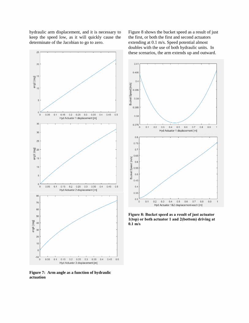
hydraulic arm displacement, and it is necessary to

keep the speed low, as it will quickly cause the

determinate of the Jacobian to go to zero.

Figure 7: Arm angle as a function of hydraulic

actuation

Figure 8 shows the bucket speed as a result of just

the first, or both the first and second actuators

extending at 0.1 m/s. Speed potential almost

doubles with the use of both hydraulic units. In

these scenarios, the arm extends up and outward.

Figure 8: Bucket speed as a result of just actuator

1(top) or both actuator 1 and 2(bottom) driving at

0.1 m/s

Similarly, acceleration potential also doubles with

the use of both actuators, shown in figure 9.

Figure 9: Bucket acceleration as a result of just

actuator 1(top) or both actuator 1 and 2(bottom)

driving at 0.1 m/s

2.7. Dynamic Results

A simple virtual work analysis was done to both

visualize power consumption of the machine, and

to validate results. In each scenario, all actuators

are moving at +/- 0.1 m/s. Figure 10 shows power

consumption of the machine over time with a full

bucket load, lowering downwards.

Figure 10: Power required to drive the arm

downwards over time – Full load in bucket

Figure 11 shows the same condition, but with the

arm moving up and out. Power consumption is

noticeably lower and more linear.

Figure 11: Power required to drive the arm up and

out over time – Full load in bucket

Figure 12 shows the consumption of the arm

moving up and out – without any mass in the

excavator bucket. The power consumption

variance is significantly lower than the scenario

with the load in the bucket.

Figure 12: Power required to drive the arm up and

out over time – No load in bucket

Each of these scenarios further validate the model.

The Link-Belt excavator used as reference has a

444 HP engine, well within the normal range of

power consumption seen in this section.

2.8. Model Limitations

The major limitation to this model is Grashof’s

criterion – or the condition in which the sum of the

shortest and longest link must remain smaller than

the sum of the remaining links in a 4 bar

mechanism. Each of the pairs of two hydraulic

links attached at the arms creates a 4 bar

mechanism, making 3 total in the entire

machine[3]. When a piston extends or retracts too

far, all links become parallel. When the piston

tries to retract further, the model fails and the

determinate of the Jacobian goes to zero. Using

the “arm up and out” movement, figure 13 shows

the Jacobian over time.

Figure 13: Jacobian over time as the arm moves up

and out

As discussed in section 2.6, with the bucket

extending the fastest, it is the most likely one to

set the determinate of the Jacobian to zero first.

3. Conclusion

A working model of an excavator arm was

successfully made and demonstrated to run in

Matlab. This could have useful applications in

determining power requirements or simulating

excavator behavior in early stages of design.

Further work on this model could include forward

dynamic analysis that would allow application of

driving forces on the prismatic joints, to better

simulate realistic hydraulic actuation.

References

[1] Link-Belt 800 LX

https://www.lbxco.com/Specs/800LX.pdf

[2] Sommer.: Notes_01_01.

[3] Sommer.: Notes_04_01

https://www.lbxco.com/Specs/800LX.pdf

% MAIN CODE

clc, clear, close all

% initialize

t=0;

tfin = 20;

proj_mass;

proj_phi;

keep = [];

keep_q = [];

keep_W = [];

assy_tol = .000001;

for t = 0 : .01 : tfin,

proj_phi;

while max(abs(PHI)) > assy_tol,

proj_phi;

q = q - inv(JAC) * PHI;

keep = [PHI';keep];

PHI;

end

t

proj_kin;

VW = -qd'*(QA-M*qdd);

keep_q = [keep_q;q'];

keep_W = [keep_W;(W1+W2+W3) t abs(VW) q(7) q(8) phi3dd sqrt(r4d'*r4d) det(JAC)];

end

%%

figure

plot(abs(dx11)*keep_W(:,2),keep_W(:,7))

xlabel('Hyd Actuator 1&2 displacement-each [m]')

ylabel('Bucket Speed [m/s]')

figure

plot(abs(dx22)*keep_W(:,2),keep_q(:,6)/pi*180 - keep_q(:,3)/pi*180)

xlabel('Hyd Actuator 2 displacement [m]')

ylabel('ang3 [deg]')

figure

plot(abs(dx33)*keep_W(:,2),keep_q(:,9)/pi*180 - keep_q(:,6)/pi*180 - keep_q(:,3)/pi*180)

xlabel('Hyd Actuator 3 displacement [m]')

ylabel('ang4 [deg]')

figure

plot(keep_W(:,2),(keep_W(:,3)*.0013412))

xlabel('Time [s]')

ylabel('Power [hp]')

figure

plot(keep_W(:,4),((keep_W(:,3))*.0013412))

xlabel('Bucket "horizontal" distance from origin [m]')


figure

plot(keep_W(:,5),((keep_W(:,3))*.0013412))

xlabel('Bucket "vertical" distance from origin [m]')


figure

plot(keep_W(:,2),keep_W(:,8))

xlabel('Time [s]')

ylabel('Det(Jac)')

%Mass or INI File

t=0;

load arm1.txt

load arm2.txt

load arm3.txt

load arm4.txt

load arm5.txt

load arm6.txt

load arm7.txt

load arm8.txt

load arm9.txt

load arm10.txt

load arm11.txt

load allglobals1.txt

load hyd1.txt

load hyd2.txt

load hyd3.txt

%Calibrate

Length = length(arm1)

pixels = sqrt((arm1(Length,1)-arm1(Length-4,1))^2 + (arm1(Length,2)-arm1(Length-4,2))^2)

%actual length = 8.73 meters

ratio = 8.73/pixels %m/pixel

%new dimensions

allglobals = allglobals1*ratio;

%scaling and moving to A as the origin

arm1 = arm1*ratio - allglobals(1,:);

arm2 = arm2*ratio- allglobals(1,:);;








arm10 = arm10*ratio- allglobals(1,:);

arm11 = arm11*ratio- allglobals(1,:);

hyd1 = hyd1*ratio-allglobals(1,:);



allglobals = allglobals-allglobals(1,:);

%flip

arm1(:,1) = arm1(:,1)*-1;

arm2(:,1) = arm2(:,1)*-1;

arm3(:,1) = arm3(:,1)*-1;

arm4(:,1) = arm4(:,1)*-1;

arm5(:,1) = arm5(:,1)*-1;

arm6(:,1) = arm6(:,1)*-1;

arm7(:,1) = arm7(:,1)*-1;

arm8(:,1) = arm8(:,1)*-1;

arm9(:,1) = arm9(:,1)*-1;

arm10(:,1) = arm10(:,1)*-1;

arm11(:,1) = arm11(:,1)*-1;

hyd1(:,1) = hyd1(:,1)*-1;

hyd2(:,1) = hyd2(:,1)*-1;

hyd3(:,1) = hyd3(:,1)*-1;

allglobals(:,1) = allglobals(:,1)*-1

plot(arm1(:,1),arm1(:,2),arm2(:,1),arm2(:,2),arm3(:,1),arm3(:,2),arm4(:,1),arm4(:,2),arm5(:,1),arm5(:,2),hyd1(:,1),hyd1(:,2),hyd2

(:,1),hyd2(:,2),hyd3(:,1),hyd3(:,2))

%Mass and CG

thick = .05;

hyd1m = 800;

hyd2m = 800;

hyd3m = 800;

m2 = 8040;

m3 = 3920;

m4 = 10000;

m5 = 100;

m6 = 100;

m7 = hyd1m/2;

m8 = hyd1m/2;

m9 = hyd2m/2;

m10 = hyd2m/2;

m11 = hyd3m/2;

m12 = hyd3m/2;

[arm1g arm1i arm1c] = polygeom((arm1(1:(length(arm1)-4),1)),(arm1(1:(length(arm1)-4),2)));





[arm6g arm6i arm6c] = polygeom(arm6(:,1),arm6(:,2));






J2 = arm1c(5)/arm1g(1);

J3 = arm2c(5)/arm2g(1);

J4 = arm3c(5)/arm3g(1);

J5 = arm4c(5)/arm4g(1);

J6 = arm5c(5)/arm5g(1);

J7 = arm6c(5)/arm6g(1);

J8 = arm7c(5)/arm7g(1);

J9 = arm8c(5)/arm8g(1);

J10 = arm9c(5)/arm9g(1);

J11 = arm10c(5)/arm10g(1);

J12 = arm11c(5)/arm11g(1);

figure

plot((arm1(1:(length(arm1)-4),1)),(arm1(1:(length(arm1)-4),2)),(arm2(1:(length(arm2)-5),1)),(arm2(1:(length(arm2)-

5),2)),(arm3(1:(length(arm3)-2),1)),(arm3(1:(length(arm3)-2),2)),(arm4(1:(length(arm4)-2),1)),(arm4(1:(length(arm4)-

2),2)),(arm5(1:(length(arm5)-2),1)),(arm5(1:(length(arm5)-

2),2)),arm6(:,1),arm6(:,2),arm7(:,1),arm7(:,2),arm8(:,1),arm8(:,2),arm9(:,1),arm9(:,2),arm10(:,1),arm10(:,2),arm11(:,1),arm11(:,2

))

hold on

%legend('1','2','3','4','5','6','7','8','9','10','11')

hold on

%Global Locations

r1A = allglobals(1,:)'

r1B = allglobals(2,:)'

r1C = allglobals(3,:)'

r1D = allglobals(4,:)'

r1E = allglobals(5,:)'

r1F = allglobals(6,:)'

r1G = allglobals(7,:)'

r1H = allglobals(8,:)'

r1I = allglobals(9,:)'

r1J = allglobals(10,:)'

r1K = allglobals(11,:)'

r1L1 = allglobals(12,:)'

r1L2 = allglobals(13,:)'

r1M2 = allglobals(14,:)'

r1M1 = allglobals(15,:)'

r1N1 = allglobals(16,:)'

r1N2 = allglobals(17,:)'

r2cg = arm1g(2:3)'

r3cg = arm2g(2:3)'

r4cg = arm3g(2:3)'

r5cg = arm4g(2:3)'

r6cg = arm5g(2:3)'

r7cg = arm6g(2:3)'

r8cg = arm7g(2:3)'

r9cg = arm8g(2:3)'

r10cg = arm9g(2:3)'

r11cg = arm10g(2:3)'

r12cg = arm11g(2:3)'

%plot(r2cg(1),r2cg(2),'*',r3cg(1),r3cg(2),'*',r4cg(1),r4cg(2),'*',r5cg(1),r5cg(2),'*',r6cg(1),r6cg(2),'*',r7cg(1),r7cg(2),'*',r8c

g(1),r8cg(2),'*',r9cg(1),r9cg(2),'*',r10cg(1),r10cg(2),'*',r11cg(1),r11cg(2),'*',r12cg(1),r12cg(2),'*')

%

s1pA = [0 0]';

s2pA = [r1A-r2cg]

s2pB = [r1B-r2cg]

s2pC = [r1C-r2cg]

s2pD = [r1D-r2cg]

s3pD = [r1D-r3cg]

s3pE = [r1E-r3cg]

s3pF = [r1F-r3cg]

s3pG = [r1G-r3cg]

s3pH = [r1H-r3cg]

s4pE = [r1E-r4cg]

s4pJ = [r1J-r4cg]

s5pF = [r1F-r5cg]

s5pI = [r1I-r5cg]

s6pI = [r1I-r6cg]

s6pJ = [r1J-r6cg]

s7pK = [r1K-r7cg]

s7pL1 = [r1L1-r7cg]

s8pL2 = [r1L2-r8cg]

s8pB = [r1B-r8cg]

s9pM2 = [r1M2-r9cg]

s9pC = [r1C-r9cg]

s10pM1 = [r1M1-r10cg]

s10pH = [r1H-r10cg]

s11pG = [r1G-r11cg]

s11pN1 = [r1N1-r11cg]

s12pN2 = [r1N2-r12cg]

s12pI = [r1I-r12cg]

%

phi2 = 0;

phi3 = 0;

phi4 = 0;

phi5 =0;

phi6 = 0;

phi7 = 0;

phi8 = 0;

phi9 = 0;

phi10 = 0;

phi11 = 0;

phi12 = 0;

q(1,1) = r2cg(1);

q(2,1) = r2cg(2);

q(3,1) = phi2;

q(4,1) = r3cg(1);

q(5,1) = r3cg(2);

q(6,1) = phi3;

q(7,1) = r4cg(1);

q(8,1) = r4cg(2);

q(9,1) = phi4;

q(10,1) = r5cg(1);

q(11,1) = r5cg(2);

q(12,1) = phi5;

q(13,1) = r6cg(1);

q(14,1) = r6cg(2);

q(15,1) = phi6;

q(16,1) = r7cg(1);

q(17,1) = r7cg(2);

q(18,1) = phi7;

q(19,1) = r8cg(1);

q(20,1) = r8cg(2);

q(21,1) = phi8;

q(22,1) = r9cg(1);

q(23,1) = r9cg(2);

q(24,1) = phi9;

q(25,1) = r10cg(1);

q(26,1) = r10cg(2);

q(27,1) = phi10;

q(28,1) = r11cg(1);

q(29,1) = r11cg(2);

q(30,1) = phi11;

q(31,1) = r12cg(1);

q(32,1) = r12cg(2);

q(33,1) = phi12;

phi2i=phi2;

phi3i=phi3;

phi4i=phi4;

%plot(allglobals(:,1),allglobals(:,2),'*')

%legend('A','B','C','D','E','F','G','H','I','J','K','L1','L2','M2','M1','N1','N2')

%Gravity

M = diag( [ m2 m2 J2*m2 m3 m3 J3*m3 m4 m4 J4*m4 m5 m5 J5*m5 m6 m6 J6*m6 m7 m7 J7*m7 m8 m8 J8*m8 m9 m9 J9*m9 m10 m10 J10*m10 m11

m11 J11*m11 m12 m12 J12*m12]);

Q2 = [0 -9.81*m2 0]';

Q3 = [0 -9.81*m3 0]';

Q4 = [0 -9.81*m4 0]';

Q5 = [0 -9.81*m5 0]';

Q6 = [0 -9.81*m6 0]';

Q7 = [0 -9.81*m7 0]';

Q8 = [0 -9.81*m8 0]';

Q9 = [0 -9.81*m9 0]';

Q10 = [0 -9.81*m10 0]';

Q11 = [0 -9.81*m11 0]';

Q12 = [0 -9.81*m12 0]';

QA = [Q2;Q3;Q4;Q5;Q6;Q7;Q8;Q9;Q10;Q11;Q12];

% PHI file

dx11 = .1;

dx22 = -.1;

dx33= .1;

%dx11 = .1;

%dx22 = -.1;

%dx33= .1;

dx1 = 1.9887 +dx11*t;

dx2 = 2.8657 +dx22*t;

dx3 = -1.9858 +dx33*t;

d2r = pi / 180;

R = [ 0 -1 ; 1 0 ];

r2 = q(1:2);

r3 = q(4:5);

r4 = q(7:8);

r5 = q(10:11);

r6 = q(13:14);

r7 = q(16:17);

r8 = q(19:20);

r9 = q(22:23);

r10 = q(25:26);

r11 = q(28:29);

r12 = q(31:32);

phi2 = q(3);

phi3 = q(6);

phi4 = q(9);

phi5 = q(12);

phi6 = q(15);

phi7 = q(18);

phi8 = q(21);

phi9 = q(24);

phi10 = q(27);

phi11 = q(30);

phi12 = q(33);

A2 = [ cos(phi2) -sin(phi2); sin(phi2) cos(phi2) ];











B2 = R * A2;

B3 = R * A3;

B4 = R * A4;

B5 = R * A5;

B6 = R * A6;

B7 = R * A7;

B8 = R * A8;

B9 = R * A9;

B10 = R * A10;

B11 = R * A11;

B12 = R * A12;

% global locations - Eq 2.4.8, page 33

r1A = [0;0];

r2A = r2 + A2*s2pA;

r2B = r2 + A2*s2pB;

r2C = r2 + A2*s2pC;

r2D = r2 + A2*s2pD;

r3D = r3 + A3*s3pD;

r3E = r3 + A3*s3pE;

r3F = r3 + A3*s3pF;

r3G = r3 + A3*s3pG;

r3H = r3 + A3*s3pH;

r4E = r4 + A4*s4pE;

r4J = r4 + A4*s4pJ;

r5F = r5 + A5*s5pF;

r5I = r5 + A5*s5pI;

r6I = r6 + A6*s6pI;

r6J = r6 + A6*s6pJ;

r7K = r7 + A7*s7pK;

r7L1 = r7 + A7*s7pL1;

r8L2 = r8 + A8*s8pL2;

r8B = r8 + A8*s8pB;

r9M2 = r9 + A9*s9pM2;

r9C = r9 + A9*s9pC;

r10M1 = r10 + A10*s10pM1;

r10H = r10 + A10*s10pH;

r11G = r11 + A11*s11pG;

r11N1 = r11 + A11*s11pN1;

r12N2 = r12 + A12*s12pN2;

r12I = r12 + A12*s12pI;

% revolute constraints - A,B,C,D - Eq 3.3.10, page 65

PHI(1:2,1) = r1A - r2A;

PHI(3:4,1) = r2B - r8B;

PHI(5:6,1) = r2C - r9C;

PHI(7:8,1) = r2D - r3D;

PHI(9:10,1) = r3E - r4E;

PHI(11:12,1) = r3F - r5F;

PHI(13:14,1) = r3G - r11G;

PHI(15:16,1) = r3H - r10H;

PHI(17:18,1) = r5I - r6I;

PHI(19:20,1) = r5I - r12I;

PHI(21:22,1) = r4J - r6J;

PHI(23:24,1) = r1K - r7K;

PHI(25,1) = transpose(r7L1-r7K)*transpose(R)*(r8B-r8L2);

PHI(26,1) = transpose(r7L1-r7K)*transpose(R)*(r8L2-r7K);

PHI(27,1) = transpose(r9M2-r9C)*transpose(R)*(r10H-r10M1);

PHI(28,1) = transpose(r9M2-r9C)*transpose(R)*(r10M1-r9C);

PHI(29,1) = transpose(r11G-r11N1)*transpose(R)*(r12N2-r12I);

PHI(30,1) = transpose(r11G-r11N1)*transpose(R)*(r12I-r11N1);

PHI(31,1) = transpose(r7L1-r7K)*(r8L2-r7K)/(sqrt((r7L1-r7K)'*(r7L1-r7K)))-dx1;

PHI(32,1) = transpose(r9M2-r9C)*(r10M1-r9C)/(sqrt((r9M2-r9C)'*(r9M2-r9C)))-dx2;

PHI(33,1) = transpose(r11G-r11N1)*(r12I-r11N1)/(sqrt((r11G-r11N1)'*(r11G-r11N1)))-dx3;

% Jacobian by rows - Eq 3.3.12, page 66 for revolutes

JAC = zeros(33,33);

JAC(1:2,1:3) = [ -eye(2) -B2*s2pA ];

JAC(3:4,1:3) = [ eye(2) B2*s2pB ];

JAC(5:6,1:3) = [ eye(2) B2*s2pC ];

JAC(7:8,1:3) = [ eye(2) B2*s2pD ];

JAC(7:8,4:6) = [ -eye(2) -B3*s3pD ];

JAC(9:10,4:6) = [ eye(2) B3*s3pE ];

JAC(11:12,4:6) = [ eye(2) B3*s3pF ];

JAC(13:14,4:6) = [ eye(2) B3*s3pG ];

JAC(15:16,4:6) = [ eye(2) B3*s3pH ];

JAC(9:10,7:9) = [ -eye(2) -B4*s4pE ];

JAC(21:22,7:9) = [ eye(2) B4*s4pJ ];

JAC(11:12,10:12) = [ -eye(2) -B5*s5pF ];

JAC(17:18,10:12) = [ eye(2) B5*s5pI ];

JAC(19:20,10:12) = [ eye(2) B5*s5pI ];

JAC(17:18,13:15) = [ -eye(2) -B6*s6pI ];

JAC(21:22,13:15) = [ -eye(2) -B6*s6pJ ];

JAC(23:24,16:18) = [ -eye(2) -B7*s7pK ];

JAC(25,16:18) = [ 0 0 -transpose(r7L1-r7K)*(r8B-r8L2) ];

JAC(26,16:18) = transpose(r7L1-r7K)*transpose(R)*-[eye(2) B7*s7pL1] - [0 0 transpose(r7L1-r7K)*(r8L2-r7K)];

JAC(3:4,19:21) = [ -eye(2) -B8*s8pB ];

JAC(25,19:21) = [ 0 0 transpose(r7L1-r7K)*(r8B-r8L2) ];

JAC(26,19:21) = transpose(r7L1-r7K)*transpose(R)*[eye(2) B8*s8pL2];

JAC(5:6,22:24) = [ -eye(2) -B9*s9pC ];

JAC(27,22:24) = [ 0 0 -transpose(r9M2-r9C)*(r10H-r10M1)];

JAC(28,22:24) = transpose(r9M2-r9C)*transpose(R)*-[eye(2) B9*s9pM2] - [0 0 transpose(r9M2-r9C)*(r10M1-r9C)];

JAC(15:16,25:27) = [ -eye(2) -B10*s10pH ];

JAC(27,25:27) = [ 0 0 transpose(r9M2-r9C)*(r10H-r10M1) ];

JAC(28,25:27) = transpose(r9M2-r9C)*transpose(R)*[eye(2) B10*s10pM1] ;

JAC(13:14,28:30) = [ -eye(2) -B11*s11pG ];

JAC(29,28:30) = [ 0 0 -transpose(r11G-r11N1)*(r12N2-r12I)];

JAC(30,28:30) = transpose(r11G-r11N1)*transpose(R)*-[eye(2) B11*s11pN1] - [0 0 transpose(r11G-r11N1)*(r12I-r11N1)];

JAC(19:20,31:33) = [ -eye(2) -B12*s12pI ];

JAC(29,31:33) = [ 0 0 transpose(r11G-r11N1)*(r12N2-r12I) ];

JAC(30,31:33) = transpose(r11G-r11N1)*transpose(R)*[eye(2) B12*s12pN2] ;

JAC(31,16:18) = [ transpose(r7L1-r7K)*-[eye(2) B7*s7pL1] + [0 0 transpose(r7L1-r7K)*transpose(R)*(r8L2-r7K)]]/(sqrt((r7L1-

r7K)'*(r7L1-r7K)));

JAC(31,19:21) = (transpose(r7L1-r7K)*[eye(2) B8*s8pL2])/(sqrt((r7L1-r7K)'*(r7L1-r7K)));

JAC(32,22:24) = [ transpose(r9M2-r9C)*-[eye(2) B9*s9pM2] + [0 0 transpose(r9M2-r9C)*transpose(R)*(r10M1-r9C)]]/(sqrt((r9M2-

r9C)'*(r9M2-r9C)));

JAC(32,25:27) = (transpose(r9M2-r9C)*[eye(2) B10*s10pM1])/(sqrt((r9M2-r9C)'*(r9M2-r9C))) ;

JAC(33,28:30) = [ transpose(r11G-r11N1)*-[eye(2) B11*s11pN1] + [0 0 transpose(r11G-r11N1)*transpose(R)*(r12I-

r11N1)]]/(sqrt((r11G-r11N1)'*(r11G-r11N1)));

JAC(33,31:33) = (transpose(r11G-r11N1)*[eye(2) B12*s12pN2])/(sqrt((r11G-r11N1)'*(r11G-r11N1))) ;

% current results

% KIN File

% velocity

velrhs = zeros(33,1);

velrhs(31) = dx11;

velrhs(32) = dx22;

velrhs(33) = dx33;

qd = inv(JAC) * velrhs;

% global velocities of points

r2d = qd(1:2);

r3d = qd(4:5);

r4d = qd(7:8);

r5d = qd(10:11);

r6d = qd(13:14);

r7d = qd(16:17);

r8d = qd(19:20);

r9d = qd(22:23);

r10d = qd(25:26);

r11d = qd(28:29);

r12d = qd(31:32);

phi2d = qd(3);

phi3d = qd(6);

phi4d = qd(9);

phi5d = qd(12);

phi6d = qd(15);

phi7d = qd(18);

phi8d = qd(21);

phi9d = qd(24);

phi10d = qd(27);

phi11d = qd(30);

phi12d = qd(33);

% acceleration

accrhs = zeros(33,1);

accrhs(1:2) = -A2*s2pA*phi2d*phi2d;

accrhs(3:4) = A2*s2pB*phi2d*phi2d - A8*s8pB*phi8d*phi8d;

accrhs(5:6) = A2*s2pC*phi2d*phi2d - A9*s9pC*phi9d*phi9d;

accrhs(7:8) = A2*s2pD*phi2d*phi2d - A3*s3pD*phi3d*phi3d;

accrhs(9:10) = A3*s3pE*phi3d*phi3d - A4*s4pE*phi4d*phi4d;

accrhs(11:12) = A3*s3pF*phi3d*phi3d - A5*s5pF*phi5d*phi5d;

accrhs(13:14) = A3*s3pG*phi3d*phi3d - A11*s11pG*phi11d*phi11d;

accrhs(15:16) = A3*s3pH*phi3d*phi3d - A10*s10pH*phi10d*phi10d;

accrhs(17:18) = A5*s5pI*phi5d*phi5d - A6*s6pI*phi6d*phi6d;

accrhs(19:20) = A5*s5pI*phi5d*phi5d - A12*s12pI*phi12d*phi12d;

accrhs(21:22) = A4*s4pJ*phi4d*phi4d - A6*s6pJ*phi6d*phi6d;

accrhs(23:24) = - A7*s7pK*phi7d*phi7d;

accrhs(25) = 0;

accrhs(26) = transpose(r7L1-r7K)*(2*phi7d*phi7d*((r8d+phi8d*B8*s8pL2)-(r7d+phi7d*B7*s7pK))+transpose(R)*(phi7d*phi7d*(r8L2-

r7K)+(phi8d*phi8d*A8*s8pL2-phi7*phi7*A7*s7pK)));

accrhs(27) = 0;

accrhs(28) = transpose(r9M2-r9C)*(2*phi9d*phi9d*((r10d+phi10d*B10*s10pM1)-(r9d+phi9d*B9*s9pC))+transpose(R)*(phi9d*phi9d*(r10M1-

r9C)+(phi10d*phi10d*A10*s10pM1-phi9*phi9*A9*s9pC)));

accrhs(29) = 0;

accrhs(30) = transpose(r11G-r11N1)*(2*phi11d*phi11d*((r12d+phi12d*B12*s12pI)-

(r11d+phi11d*B11*s11pN1))+transpose(R)*(phi11d*phi11d*(r12I-r11N1)+(phi12d*phi12d*A12*s12pI-phi11*phi11*A11*s11pN1)));

accrhs(31)=transpose(r7L1-r7K)*(-2*phi7d*phi7d*transpose(R)*((r8d+phi8d*B8*s8pL2)-(r7d+phi7d*B7*s7pK))+phi7d*phi7d*(r8L2-

r7K)+(phi8d*phi8d*A8*s8pL2-phi7*phi7*A7*s7pK))/(sqrt((r7L1-r7K)'*(r7L1-r7K)));;

accrhs(32)=transpose(r9M2-r9C)*(-2*phi9d*phi9d*transpose(R)*((r10d+phi10d*B10*s10pM1)-(r9d+phi9d*B9*s9pC))+phi9d*phi9d*(r8L2-

r7K)+(phi10d*phi10d*A10*s10pM1-phi9*phi9*A9*s9pC))/(sqrt((r9M2-r9C)'*(r9M2-r9C)));;

accrhs(33)=transpose(r11G-r11N1)*(-2*phi11d*phi11d*transpose(R)*((r12d+phi12d*B12*s12pI)-

(r11d+phi11d*B11*s11pN1))+phi9d*phi9d*(r8L2-r7K)+(phi12d*phi12d*A12*s12pI-phi11*phi11*A11*s11pN1))/(sqrt((r11G-r11N1)'*(r11G-

r11N1)));;

qdd = inv(JAC) * accrhs;

% global accelerations

r2dd = qdd(1:2);

r3dd = qdd(4:5);

r4dd = qdd(7:8);

phi2dd = qdd(3);

phi3dd = qdd(6);

phi4dd = qdd(9);

%Force

lambda = inv(JAC') * ( QA - M*qdd );

%F1 = norm(r7L1-r7K)*norm(r8L2-r7K)*lambda(26);

%F2 = norm(r9M2-r9C)*norm(r10M1-r9C)*lambda(28);

%F3 = norm(r11G-r11N1)*norm(r12I-r11N1)*lambda(30);

%F1 = R*(r7L1-r7K)*lambda(26);

%F2 = R*(r9M2-r9C)*lambda(28);

%F3 = R*(r11G-r11N1)*lambda(30);

F1 = -lambda(3:4);

F2 = -lambda(15:16);

F3 = -lambda(19:20);

W1 = sqrt(F1'*F1)*(abs(dx11));



1

MANUFACTURING A SPHERICAL FOUR-BAR MECHANISM

Ritika Menghani and Ellen Zerbe

Pennsylvania State University, State College, PA

ABSTRACT Students are very familiar with the standard planar four bar

mechanism. A spherical four bar would assist in the transition to

three dimensions by starting with a familiar design. The

spherical four bar is also unique in that while it operates in three

dimension in an x-y-z coordinate frame, it only operates in two

dimensions when considering a spherical coordinate frame (ϕ

and θ). The links for the mechanism were manufactured using

3D printing because it was the simplest and least expensive

method for creating the geometry needed.

INTRODUCTION Spherical four-bar mechanisms are similar to the more

common planar four-bar mechanism in that they are created by

four links with four revolute joints connecting them. When the

axes of rotation for each revolute intersect at a single point, the

mechanism is considered a spherical four-bar. The links then

travel a path that lies on the surface of a sphere as the mechanism

moves. These linkages are often used to replace multiple joints

in instances where a more fluid motion is desired. The controlled

motion of a spherical four-bar can be better than any

unsteadiness that results from multiple joints. The folding

mechanism on small airplane wings is an example of this.

Some work has already been done on the design of spherical

four-bars using standard manufacturing methods [1] and

specialized design software [2]. We decided to use additive

manufacturing due to its ability to create complex geometry, its

cost effectiveness, and its speed of manufacturing.

MATERIALS AND METHODS Each piece of the spherical four-bar mechanism was

modelled in SolidWorks and then printed using PLA. The

designs were based off of an available spherical four-bar model

on YouMagine [3]. Modifications were made in the redesigned

pieces to better fit the intended joint system, ie: replacing snap

fits with through hole. All four links and base connector were

printed using the Mechanical Engineering department’s 3D

printing services. The final iteration of the base was printed with

a personal 3D printer where the layer thickness and infill density

could be more controlled. A picture of the final assembly is

shown in Figure 1.

FIGURE 1: Final assembly of the spherical four-bar mechanism.

RESULTS AND DISCUSSION 3D printing some of the parts required multiple iterations,

specially the base. Due to 3D printers generally undersizing

holes, the base connector would not fit into the base and hence

this required a little bit of redesign and reprinting. Figure 2 shows

the iterations of the base.

FIGURE 2: Three printings of the base part. The orange piece was

printed using the me department printing services and the piece on the

right was the final product.

Another challenge encountered in this project was the

stacking. Initially, standard machine bolts were selected as the

joints between links, however, the bolt head ended up interfering

with the motion of the links. This was resolved by using carriage

bolts which have a smaller head and allow full motion of all

links. Figure 3 demonstrates the stacking issue and result when

the bolts were switched.

2

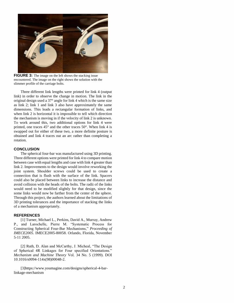
FIGURE 3: The image on the left shows the stacking issue

encountered. The image on the right shows the solution with the

slimmer profile of the carriage bolts.

Three different link lengths were printed for link 4 (output

link) in order to observe the change in motion. The link in the

original design used a 37° angle for link 4 which is the same size

as link 2; link 1 and link 3 also have approximately the same

dimensions. This leads a rectangular formation of links, and

when link 2 is horizontal it is impossible to tell which direction

the mechanism is moving in if the velocity of link 2 is unknown.

To work around this, two additional options for link 4 were

printed, one traces 45° and the other traces 50°. When link 4 is

swapped out for either of these two, a more definite posture is

obtained and link 4 traces out an arc rather than completing a

rotation.

CONCLUSION The spherical four-bar was manufactured using 3D printing.

Three different options were printed for link 4 to compare motion

between case with equal lengths and case with link 4 greater than

link 2. Improvements to the design would involve reworking the

joint system. Shoulder screws could be used to create a

connection that is flush with the surface of the link. Spacers

could also be placed between links to increase the distance and

avoid collision with the heads of the bolts. The radii of the links

would need to be modified slightly for that design, since the

some links would now be farther from the center of the sphere.

Through this project, the authors learned about the limitations of

3D printing tolerances and the importance of stacking the links

of a mechanism appropriately.

REFERENCES [1] Turner, Michael L., Perkins, David A., Murray, Andrew

P., and Larochelle, Pierre M. “Systematic Process for

Constructing Spherical Four-Bar Mechanisms,” Proceeding of

IMECE2005. IMECE2005-80058. Orlando, Florida, November

5-11 2005.

[2] Ruth, D. Alan and McCarthy, J. Micheal, “The Design

of Spherical 4R Linkages for Four specified Orientations.”

Mechanism and Machine Theory Vol. 34 No. 5 (1999). DOI

10.1016/s0094-114x(98)00048-2.

[3]https://www.youmagine.com/designs/spherical-4-bar-

linkage-mechanism

1

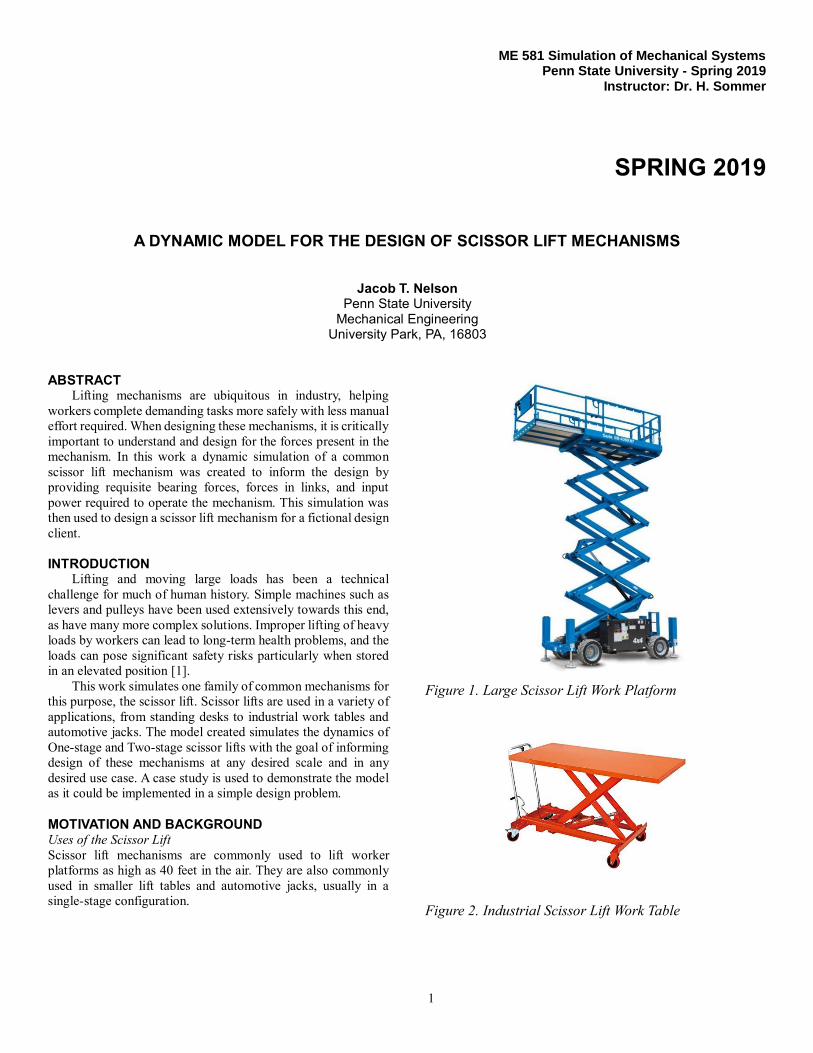
ME 581 Simulation of Mechanical Systems Penn State University - Spring 2019

Instructor: Dr. H. Sommer

SPRING 2019

A DYNAMIC MODEL FOR THE DESIGN OF SCISSOR LIFT MECHANISMS

Jacob T. Nelson Penn State University

Mechanical Engineering University Park, PA, 16803

ABSTRACT Lifting mechanisms are ubiquitous in industry, helping

workers complete demanding tasks more safely with less manual

effort required. When designing these mechanisms, it is critically

important to understand and design for the forces present in the

mechanism. In this work a dynamic simulation of a common

scissor lift mechanism was created to inform the design by

providing requisite bearing forces, forces in links, and input

power required to operate the mechanism. This simulation was

then used to design a scissor lift mechanism for a fictional design

client.

INTRODUCTION Lifting and moving large loads has been a technical

challenge for much of human history. Simple machines such as

levers and pulleys have been used extensively towards this end,

as have many more complex solutions. Improper lifting of heavy

loads by workers can lead to long-term health problems, and the

loads can pose significant safety risks particularly when stored

in an elevated position [1].

This work simulates one family of common mechanisms for

this purpose, the scissor lift. Scissor lifts are used in a variety of

applications, from standing desks to industrial work tables and

automotive jacks. The model created simulates the dynamics of

One-stage and Two-stage scissor lifts with the goal of informing

design of these mechanisms at any desired scale and in any

desired use case. A case study is used to demonstrate the model

as it could be implemented in a simple design problem.

MOTIVATION AND BACKGROUND Uses of the Scissor Lift

Scissor lift mechanisms are commonly used to lift worker

platforms as high as 40 feet in the air. They are also commonly

used in smaller lift tables and automotive jacks, usually in a

single-stage configuration.

Figure 1. Large Scissor Lift Work Platform

Figure 2. Industrial Scissor Lift Work Table

2

Figure 3. Scissor Lift mechanism used in an Adjustable

Standing Desk

Additionally, several standing desk designs utilize a scissor

lift mechanism on a smaller scale, allowing a desk top and

attached hardware such as a computer to move vertically and

provide a stable work platform for office use.

Scissor Lift Mechanism Operation

The term “scissor lift” is traditionally used in reference to a

type of work platform, capable of changing its height using a

series of members joined at their center with a revolute to create

an X shape. [2]–[4] These members rotate relative to one another

to change the height of the mechanism. These X-shaped

members can then be stacked to give the mechanism the ability

to lift the platform higher. The basic mechanism is illustrated in

Figure 4. Each set of X-shaped members is referred to as a

“stage.” A scissor lift with only a single stage has two members

joined at their center, and to the platform above.

Figure 4. 1-stage Scissor Lift Mechanism

Scissor lift mechanisms can be modeled using a pin-in-slot

joint opposite a revolute joint on both the platform and the base,

which is represented in this model as ground. Both pin-in-slot

joints are located on the same side.

The mechanism has a single degree of freedom, capable of

moving in the vertical direction only. The one-stage case has four

links, three revolute joints, and two pin-in-slot joints.

𝑀 = 3(4 − 1) − 2(3) − 2 = 1 (1 𝑠𝑡𝑎𝑔𝑒)

𝑀 = 6(6 − 1) − 2(6) − 2 = 1 (2 𝑠𝑡𝑎𝑔𝑒)

These mechanisms can be driven in a variety of ways. One

simple way is to place a hydraulic or pneumatic actuator between

two joints on different links, changing the distance between the

two points. Motors can also be used to control the angle at the

ground revolute A, though this method is limited by the motor’s

holding torque which is responsible for keeping the load

elevated.

DESIGN PARAMETERS AND MODEL OUTPUTS To inform the design of these types of mechanisms, a

dynamic model was created. The inputs to this model are the

member link lengths (L2, L3, L4), the center of gravity position

of each link (default is centered in the link), and the loading

scenario of the table (a load in kg and the distance from center).

The model then outputs the forces in each link, the forces in the

bearings, and the motion of the various joints. The maximum

range of the mechanism is defined by Φ2, which operates

between 0 degrees and less than 90 degrees. At 90 degrees the

pin-in-slot joint E is located at the same planar position as joint

D. This represents an extreme case, as most scissor lifts operate

with Φ2 between 0 degrees and 60 degrees, as at 60 degrees joint

E is located at or near the center of the table, Link 4. This creates

stability concerns if the center of gravity is located at the center.

Table 1. List of design parameters for 1-stage mechanism

Sym. Parameter Units

L2 Link 2 Length m

L3 Link 3 Length m

L4 Link 4 Length m

CG Link Center of Gravity m

ω2 Rotational speed L2 Rad/s

Load Mass on platform kg

LP Load position from

center (+ right)

m

A link’s geometric and mass parameters can also be defined.

Each link has a width and a thickness, with the assumption that

each link is rectangular. The width represents the size of the face

of the link (that is, the side visible in Figure 6) while the

thickness represents the depth, the dimension into the page.

3

Because the mechanism is assumed to be symmetrical, the side

of the mechanism being analyzed is assumed to be carrying half

of the mass of the table, and thus the thickness of the table is

divided by two for the calculation.

Assumptions and Constraints

It is assumed that the mechanism is symmetrical, with an

identical support on the opposite side in three dimensions. The

model also assumes that links are perfectly rigid, so no

deformation is possible.

SINGLE-STAGE SCISSOR LIFT As described previously the scissor lift mechanism has one

degree of freedom, straight up and down in the y-direction. A

perfectly rigid mechanism should allow no table motion in the

global x-direction.

The joint and link definitions are shown in Figure 5. The single

stage scissor lift has three revolute joints at point A, C, and D.

Two pin-in-slot joints at B and E allow the mechanism to move

up and down. Link 1 is ground, Links 2 and 3 are the main

supports, and Link 4 is the table top.

Figure 5. Labeled 1-stage scissor lift as used in model

Figure 6 shows the parameters used to define each link. Local

coordinate frames are defined at the link center of gravity. The

center of gravity position can be defined at any point by

modifying the LiG value. The central pivot, joint C, is always

located at the center of the link, at half of Li.

Figure 6. Link Parameters and Local Coordinate Frames

Local body-fixed coordinates are defined using the parameters

Li and LiG, with these parameters defined from the left-most joint

(Joints A and D respectively). Calculations for link 2 are shown

for example:

{𝑠2}′𝐴 = { −𝐿2𝐺 , 0 }

{𝑠2}′𝐶 = {

𝐿22− 𝐿2𝐺 , 0 }

{𝑠2}′𝐸 = { 𝐿2 − 𝐿2𝐺 , 0 }

Global coordinate frames are also defined using these

parameters.

{𝑟2} = { 𝐿2𝐺 cos(𝜙2) , 𝐿2𝐺 sin(𝜙2) } {𝑟3} = { (𝐿3 − 𝐿3𝐺) cos(2𝜋 − 𝜙3) , (𝐿3 − 𝐿3𝐺) sin(2𝜋 − 𝜙3) } {𝑟4} = { 𝐿4𝐺 , 𝐿2 sin(𝜙2) }

There are 9 generalized coordinates for the single stage

mechanism.

{𝑞} =

{

𝑟2𝜙2𝑟3𝜙3𝑟4𝜙4}

The following equation shows the constraint vector for the single

stage case, with eight kinematic constraints and one driver

constraint:

{𝜙} =

{

{𝑟2}𝐴 − {𝑟1}

𝐴

{𝑎1}𝑇[𝑅]𝑇{𝑑13}

{𝑟2}𝐶 − {𝑟3}

𝐶

{𝑟4}𝐷 − {𝑟3}

𝐷

{𝑎4}𝑇[𝑅]𝑇{𝑑42}

𝜙2 −𝜙2𝑠𝑡𝑎𝑟𝑡 − 𝜔2𝑡}

𝑅𝑒𝑣𝐴𝑃𝑖𝑛𝑆𝑙𝑜𝑡𝐵𝑅𝑒𝑣𝐶𝑅𝑒𝑣𝐷

𝑃𝑖𝑛𝑆𝑙𝑜𝑡𝐸𝐷𝑟𝑖𝑣𝑒𝑟

For this simulation a relatively simple relative angle driver was

used at joint A, simulating a mechanism driven by an electric

4

motor. Other drivers simulating hydraulic actuators would be

possible, but were not implemented in this model.

With 9 generalized coordinates and 9 constraints, the

mechanism’s Jacobian is a 9x9 matrix.

[Φ]𝑟𝑒𝑣𝐴 = [ [𝐼2] [𝐵2]{𝑠2}′𝐴 ]

[Φ]𝑝𝑖𝑛𝑆𝑙𝑜𝑡𝐵 = [ {𝑎1}𝑇[𝑅]𝑇[𝐼2] {𝑎1}

𝑇[𝑅]𝑇[𝐵3]{𝑠3}′𝐵 ]

[Φ]𝑟𝑒𝑣𝐶,2 = [ [𝐼2] [𝐵2]{𝑠2}′𝐶 ]

[Φ]𝑟𝑒𝑣𝐶,3 = −[ [𝐼2] [𝐵3]{𝑠3}′𝐶 ]

[Φ]𝑟𝑒𝑣𝐷,4 = [ [𝐼2] [𝐵4]{𝑠4}′𝐷 ]

[Φ]𝑟𝑒𝑣𝐷,3 = −[ [𝐼2] [𝐵3]{𝑠3}′𝐷 ]

[Φ]𝑝𝑖𝑛𝑆𝑙𝑜𝑡𝐸,4 = [ {𝑎4}𝑇[𝑅]𝑇[ [𝐼2] [𝐵2]{𝑠2}

′𝐶 ]

− [01𝑥2 {𝑎4}𝑇{𝑑42} ] ]

[Φ]𝑝𝑖𝑛𝑆𝑙𝑜𝑡𝐸,2 = [ {𝑎4}𝑇[𝑅]𝑇[𝐼2] {𝑎4}

𝑇[𝑅]𝑇[𝐵2]{𝑠2}′𝐶 ]

[Φ]𝑑𝑟𝑖𝑣𝑒𝑟 = [ [01𝑥2] 1 [01𝑥2] 0 [01𝑥2] 0 ]

Where: {𝑎1} = {𝑟1}

𝐴 − {𝑟1}𝑃 {𝑑13} = {𝑟3}

𝐵 − {𝑟1}𝐴

And:

{𝑎4} = {𝑟4}𝐷 − {𝑟4}

𝐹 {𝑑42} = {𝑟2}𝐸 − {𝑟4}

𝐹

A Newton-Raphson algorithm was used to solve the Jacobian

and calculate the kinematic position solution. Velocity and

acceleration solutions were then computed using the following

equations.

Velocity Solutions

𝑣𝑘𝑖𝑛𝑒𝑚𝑎𝑡𝑖𝑐 = {01𝑥8} 𝑣𝑑𝑟𝑖𝑣𝑒𝑟 = 𝜔2

Acceleration Solutions

𝛾𝑟𝑒𝑣𝐴 = [𝐴2]{𝑠2}′𝐴𝜙2

2̇

𝛾𝑝𝑖𝑛𝑆𝑙𝑜𝑡𝐵 = {𝑎1}𝑇[𝑅]𝑇(−𝜙3

2̇ [𝐴3]{𝑠2}′𝐴)

𝛾𝑟𝑒𝑣𝐶 = [𝐴3]{𝑠3}′𝐶𝜙3

2̇ − [𝐴2]{𝑠2}′𝐶𝜙2

2̇

𝛾𝑟𝑒𝑣𝐷 = [𝐴4]{𝑠4}′𝐶𝜙4

2̇ − [𝐴3]{𝑠3}′𝐷𝜙3

2̇

𝛾𝑝𝑖𝑛𝑆𝑙𝑜𝑡𝐸 = {𝑎4}𝑇(2𝜙4̇{𝑑42} + 𝑅𝑇(𝜙4

2̇̇ {𝑑42} + 𝜙22̇ [𝐴2]{𝑠2}

′𝐸

−𝜙42[𝐴4]{𝑠4}

′𝐸)) 𝛾𝐷𝑟𝑖𝑣𝑒𝑟 = 0

Dynamic Solution

The mass of each link can be calculated as follows, assuming

each link is rectangular:

𝑚𝑖 = 𝐿𝑖𝑤𝑑𝑖𝑡ℎ𝑖𝜌

Where 𝜌 is the density of the material, in kg/m3. All lengths are

measured in meters.

Next, mass moment of inertia is calculated, again assuming all

links are rectangular.

𝐽𝑖 = (1

12)𝑚𝑖(𝐿𝑖

2 +𝑤𝑑𝑖2)

Mass matrices are assembled for each link, and then compiled

into the mass matrix for the full mechanism.

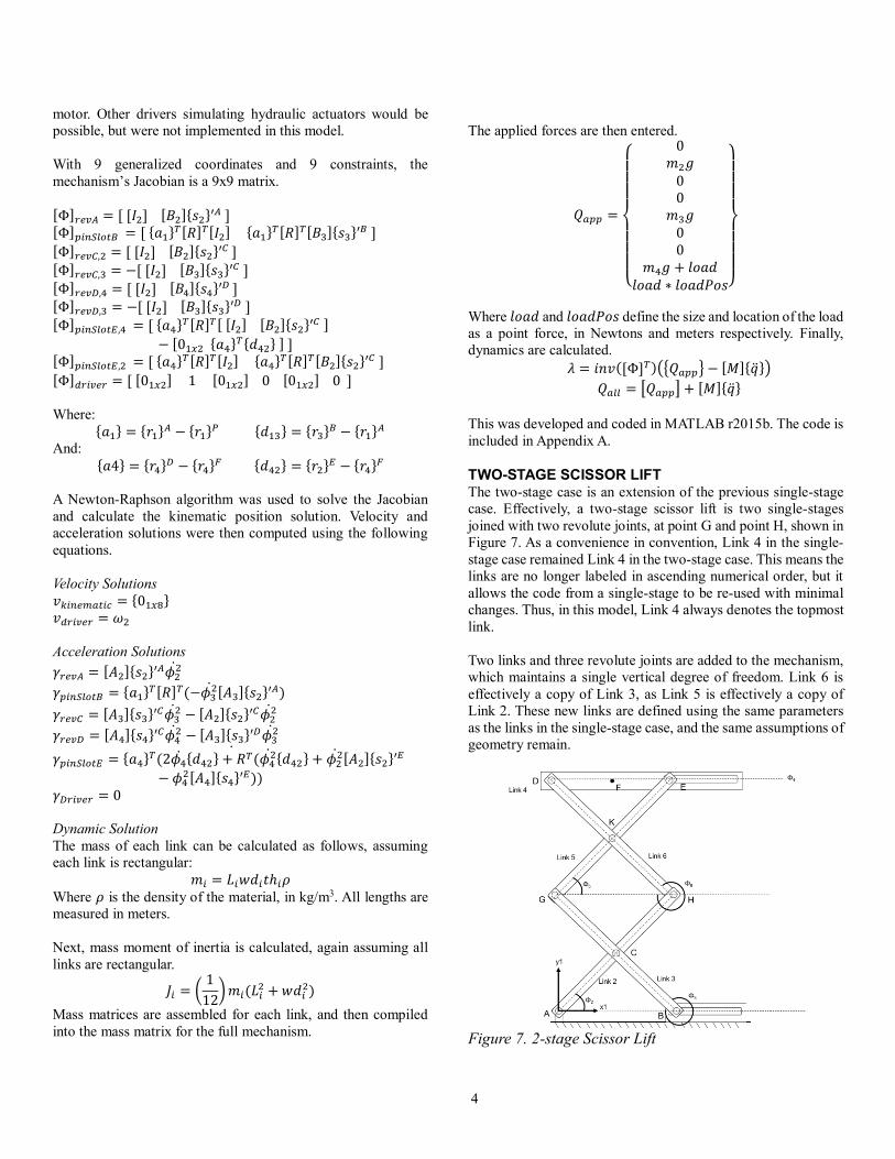
The applied forces are then entered.

𝑄𝑎𝑝𝑝 =

{

0𝑚2𝑔00𝑚3𝑔00

𝑚4𝑔 + 𝑙𝑜𝑎𝑑𝑙𝑜𝑎𝑑 ∗ 𝑙𝑜𝑎𝑑𝑃𝑜𝑠}

Where 𝑙𝑜𝑎𝑑 and 𝑙𝑜𝑎𝑑𝑃𝑜𝑠 define the size and location of the load

as a point force, in Newtons and meters respectively. Finally,

dynamics are calculated.

𝜆 = 𝑖𝑛𝑣([Φ]𝑇)({𝑄𝑎𝑝𝑝} − [𝑀]{�̈�})

𝑄𝑎𝑙𝑙 = [𝑄𝑎𝑝𝑝] + [𝑀]{�̈�}

This was developed and coded in MATLAB r2015b. The code is

included in Appendix A.

TWO-STAGE SCISSOR LIFT The two-stage case is an extension of the previous single-stage

case. Effectively, a two-stage scissor lift is two single-stages

joined with two revolute joints, at point G and point H, shown in

Figure 7. As a convenience in convention, Link 4 in the single-

stage case remained Link 4 in the two-stage case. This means the

links are no longer labeled in ascending numerical order, but it

allows the code from a single-stage to be re-used with minimal

changes. Thus, in this model, Link 4 always denotes the topmost

link.

Two links and three revolute joints are added to the mechanism,

which maintains a single vertical degree of freedom. Link 6 is

effectively a copy of Link 3, as Link 5 is effectively a copy of

Link 2. These new links are defined using the same parameters

as the links in the single-stage case, and the same assumptions of

geometry remain.

Figure 7. 2-stage Scissor Lift

5

After adding the new links, the mechanism now requires 15

generalized coordinates and 15 total constraints.

{𝑞} =

{

𝑟2𝜙2𝑟3𝜙3𝑟5𝜙5𝑟6𝜙6𝑟4𝜙4}

{𝜙} =

{

{𝑟2}𝐴 − {𝑟1}

𝐴

{𝑎1}𝑇[𝑅]𝑇{𝑑13}

{𝑟2}𝐶 − {𝑟3}

𝐶

{𝑟5}𝐺 − {𝑟3}

𝐺

{𝑟6}𝐻 − {𝑟2}

𝐻

{𝑟6}𝐾 − {𝑟5}

𝐾

{𝑟6}𝐷 − {𝑟4}

𝐷

{𝑎4}𝑇[𝑅]𝑇{𝑑45}

𝜙2 −𝜙2𝑠𝑡𝑎𝑟𝑡 − 𝜔2𝑡}

𝑅𝑒𝑣𝐴𝑃𝑖𝑛𝑆𝑙𝑜𝑡𝐵𝑅𝑒𝑣𝐶𝑅𝑒𝑣𝐺𝑅𝑒𝑣𝐻𝑅𝑒𝑣𝐾𝑅𝑒𝑣𝐷

𝑃𝑖𝑛𝑆𝑙𝑜𝑡𝐸𝐷𝑟𝑖𝑣𝑒𝑟

The new Jacobian should be 15 rows by 15 columns. The

Jacobian terms for the new mechanism are shown as below:

[Φ]𝑟𝑒𝑣𝐴 = [ [𝐼2] [𝐵2]{𝑠2}′𝐴 ]

[Φ]𝑝𝑖𝑛𝑆𝑙𝑜𝑡𝐵 = [ {𝑎1}𝑇[𝑅]𝑇[𝐼2] {𝑎1}

𝑇[𝑅]𝑇[𝐵3]{𝑠3}′𝐵 ]

[Φ]𝑟𝑒𝑣𝐶,2 = [ [𝐼2] [𝐵2]{𝑠2}′𝐶 ]

[Φ]𝑟𝑒𝑣𝐶,3 = −[ [𝐼2] [𝐵3]{𝑠3}′𝐶 ]

[Φ]𝑟𝑒𝑣𝐺,5 = [ [𝐼2] [𝐵5]{𝑠5}

′𝐺 ] [Φ]𝑟𝑒𝑣𝐺,3 = −[ [𝐼2] [𝐵3]{𝑠3}

′𝐺 ] [Φ]𝑟𝑒𝑣𝐻,6 = [ [𝐼2] [𝐵6]{𝑠6}

′𝐻 ] [Φ]𝑟𝑒𝑣𝐻,2 = −[ [𝐼2] [𝐵2]{𝑠2}

′𝐻 ] [Φ]𝑟𝑒𝑣𝐾,5 = [ [𝐼2] [𝐵5]{𝑠5}

′𝐾 ] [Φ]𝑟𝑒𝑣𝐾,6 = −[ [𝐼2] [𝐵6]{𝑠6}

′𝐾 ] [Φ]𝑟𝑒𝑣𝐷,6 = [ [𝐼2] [𝐵6]{𝑠6}

′𝐷 ] [Φ]𝑟𝑒𝑣𝐷,4 = −[ [𝐼2] [𝐵4]{𝑠4}

′𝐷 ] [Φ]𝑝𝑖𝑛𝑆𝑙𝑜𝑡𝐸,4 = [ {𝑎4}

𝑇[𝑅]𝑇[ [𝐼2] [𝐵5]{𝑠5}′𝐶 ]

− [01𝑥2 {𝑎4}𝑇{𝑑45} ] ]

[Φ]𝑝𝑖𝑛𝑆𝑙𝑜𝑡𝐸,5 = [ {𝑎4}𝑇[𝑅]𝑇[𝐼2] {𝑎4}

𝑇[𝑅]𝑇[𝐵5]{𝑠5}′𝐶 ]

[Φ15,3]𝑑𝑟𝑖𝑣𝑒𝑟 = 1

Where:

{𝑎1} = {𝑟1}𝐴 − {𝑟1}

𝑃 {𝑑13} = {𝑟3}𝐵 − {𝑟1}

𝐴

And: {𝑎4} = {𝑟4}

𝐷 − {𝑟4}𝐹 {𝑑45} = {𝑟5}

𝐸 − {𝑟4}𝐹

Again, a Newton-Raphson algorithm was used to determine the

position solution, and velocity and acceleration solutions were

then computed.

Velocity Solutions

𝑣𝑘𝑖𝑛𝑒𝑚𝑎𝑡𝑖𝑐 = {01𝑥14} 𝑣𝑑𝑟𝑖𝑣𝑒𝑟 = 𝜔2

Acceleration Solutions

𝛾𝑟𝑒𝑣𝐴 = [𝐴2]{𝑠2}′𝐴𝜙2

2̇

𝛾𝑝𝑖𝑛𝑆𝑙𝑜𝑡𝐵 = {𝑎1}𝑇[𝑅]𝑇(−𝜙3

2̇ [𝐴3]{𝑠2}′𝐴)

𝛾𝑟𝑒𝑣𝐶 = [𝐴3]{𝑠3}′𝐶𝜙3

2̇ − [𝐴2]{𝑠2}′𝐶𝜙2

2̇

𝛾𝑟𝑒𝑣𝐺 = [𝐴5]{𝑠5}′𝐺𝜙5

2̇ − [𝐴3]{𝑠3}′𝐺𝜙3

2̇

𝛾𝑟𝑒𝑣𝐻 = [𝐴6]{𝑠6}′𝐻𝜙6

2̇ − [𝐴2]{𝑠2}′𝐻𝜙2

2̇

𝛾𝑟𝑒𝑣𝐾 = [𝐴6]{𝑠6}′𝐾𝜙6

2̇ − [𝐴5]{𝑠5}′𝐾𝜙5

2̇

𝛾𝑟𝑒𝑣𝐷 = [𝐴4]{𝑠4}′𝐶𝜙4

2̇ − [𝐴6]{𝑠6}′𝐷𝜙6

2̇

𝛾𝑝𝑖𝑛𝑆𝑙𝑜𝑡𝐸 = {𝑎4}𝑇(2𝜙4̇{𝑑45} + 𝑅𝑇(𝜙4

2̇̇ {𝑑45} + 𝜙52̇ [𝐴5]{𝑠5}

′𝐸

−𝜙42[𝐴4]{𝑠4}

′𝐸)) 𝛾𝐷𝑟𝑖𝑣𝑒𝑟 = 0

Mass calculations are the same as for the single-stage case. The

new applied force vector contains two new terms.

𝑄𝑎𝑝𝑝 =

{

0𝑚2𝑔00𝑚3𝑔00𝑚5𝑔00𝑚6𝑔00

𝑚4𝑔 + 𝑙𝑜𝑎𝑑𝑙𝑜𝑎𝑑 ∗ 𝑙𝑜𝑎𝑑𝑃𝑜𝑠}

Dynamic calculations also remain the same as before.

𝜆 = 𝑖𝑛𝑣(𝐽𝐴𝐶𝑇)({𝑄𝑎𝑝𝑝} − [𝑀]{�̈�})

𝑄𝑎𝑙𝑙 = [𝑄𝑎𝑝𝑝] + [𝑀]{�̈�}

The full code for the 2-stage mechanism can be found in

Appendix B.

CASE STUDY: To test the model developed in its role as a design tool, a simple

design prompt was created. The prompt was:

A company wants to design a mobile lift

table to lift heavy equipment weighing up

to 1500 pounds. They need to lift these

loads from the floor to a maximum height

of 1.5 meters. They need to determine the

power required from an electric motor to

evaluate the feasibility of an electric

6

design, as well as the forces in all links

and bearings to use appropriate

hardware.

Table 2 shows the parameters and values used in the simulation

of the single-stage scissor lift to address the design prompt.

Table 2. Parameters used for single-stage simulation

Parameter Value Parameter Value

Load 1500 kg Material Steel

Req. Height 1.5 m Mat.

Density

7850 kg/m3

L2 1.75 m Drive Type Electric

motor

L3 1.75 m Drive

location(s)

Φ2

L4 2.0 m Drive Speed 0.1 rad/s

wd2 0.05 m Φ2_start 0 deg

wd3 0.05 m Φ2_finish 60 deg

wd4 0.05 m th3 0.01 m

th2 0.01 m th4 1.0 m

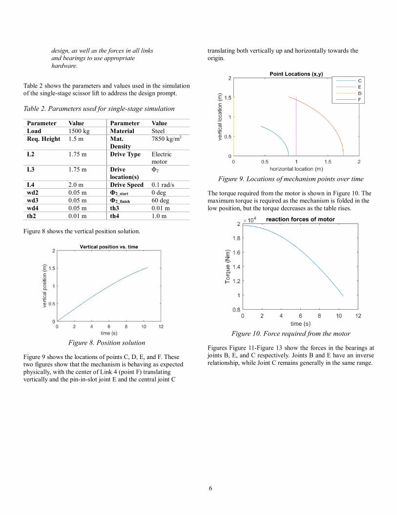
Figure 8 shows the vertical position solution.

Figure 8. Position solution

Figure 9 shows the locations of points C, D, E, and F. These

two figures show that the mechanism is behaving as expected

physically, with the center of Link 4 (point F) translating

vertically and the pin-in-slot joint E and the central joint C

translating both vertically up and horizontally towards the

origin.

Figure 9. Locations of mechanism points over time

The torque required from the motor is shown in Figure 10. The

maximum torque is required as the mechanism is folded in the

low position, but the torque decreases as the table rises.

Figure 10. Force required from the motor

Figures Figure 11-Figure 13 show the forces in the bearings at

joints B, E, and C respectively. Joints B and E have an inverse

relationship, while Joint C remains generally in the same range.

7

Figure 11. Reaction forces of the pin-in-slot joint B

Figure 12. Reaction forces of pin-in slot joint at E

Figure 13. Reaction forces at Joint C

Table 3. Table of forces in links and forces at each joint

Joint Max Force (N) Max Bearing

Force (N)

A, x 0.0601 10.36

A, y 67.43 18,067

B 0 3,362

C, x 0.0601 10.33

C, y 67.43 13,517

D, x 0.0608 10.30

D, y 10.30 6724.8

E 11,216 6892.8

Motor 1.2 19,732

Table 3 shows the maximum forces in links and bearing forces

at each joint in the mechanism. The key takeaway in this case is

the torque required from the motor, at 19.7 kNm. Using the

following equation, the power requirement can be calculated.

𝑃 =∑𝑇

𝑡= 314 𝑘𝑊

While it is not impossible to achieve these specifications with

electric motors, hydraulic actuators would likely provide a better

and potentially more economical solution for this use case.

Two-stage comparison

Using this model stage configurations can be compared to find if

one configuration is more efficient than another. For this case

study, a two-stage mechanism was compared with the single-

stage results.

The table, link 4, remains 2.0 m, but link 2, 3, 5, and 6 are

reduced in length to 1.0 m. All other parameters remain

unchanged from those in Table 2. The vertical position solution

is shown in Figure 14.

Figure 14. Vertical position vs. time for 2-stage case

8

The torque required from the motor is shown in Figure 15.

While following a similar profile to the single-stage case, more

torque is required at the initial stages of the lift.

Figure 15. Two-stage reaction forces at motor

Figure 16 and Figure 17 show the reaction forces at joint B and

joint C. Again, the reactions at joint B follow a similar trend as

the single-stage case, but the reactions at joint C change more

rapidly and more severely.

Figure 16. Two-stage reaction forces at joint B

Figure 17. Two-stage reaction forces at joint C

Table 4. Results from the two-stage case

Joint Max Force (N) Max Bearing

Force (N)

A, x 0.0196 12.55

A, y 38.52 28,249

B 0 8,443.8

C, x 0.0196 6.44 x 105

C, y 38.52 22,568

G, x 0.0118 6.44 x 105

G, y 0.0714 5641.5

H, x 38.59 6.44 x 105

H, y 0 7602.9

K, x 0.0714 6.44 x 105

K, y 38.59 3909.9

D, x 0.0118 12.39

D, y 12.39 5603

E 11,219 2514

Motor 0.771 22566

Power Requirement 354.2 kW

There is no appreciable benefit to using a two-stage

configuration over a single-stage configuration, as the two-stage

case requires more torque and more power using these

parameters. While the two—stage case could likely be optimized

further, the two still perform similarly.

Limitations

There are several ways to improve the case study and model

used. This work uses rough approximations of link parameters,

likely leading to an overestimation of mass in the system,

increasing power and torque requirements. This case study and

model used a simple rectangular shape for the links of the

mechanism, though it may be useful to incorporate other

common shapes for metal members, such as round or square

tube.

9

CONCLUSION AND FUTURE WORK This work presents a dynamic model of one-stage and two-

stage scissor lift mechanisms and utilizes the model in a

hypothetical design situation. Designs utilizing a one-stage and

two-stage configuration are compared, finding that in the design

case presented, a two-stage configuration has no appreciable

benefit over a single-stage design.

The model can easily be expanded to simulate n-stage

scissor lift mechanisms, giving more configuration options for a

designer. Another interesting simulation would use forward

dynamics to simulate the results of component failure, either of

the driver or a joint. This, coupled with extreme loading

scenarios, could allow for an assessment of risk should particular

components fail. Finally, more driver options could be

incorporated, particularly simulating hydraulic actuators

between two of the links, giving the ability to compare the results

using different drivers.

ACKNOWLEDGMENTS I would like to thank Dr. Sommer for his instruction this

semester and the Penn State Department of Mechanical

Engineering for creating these educational opportunities.

REFERENCES [1] OSHA, “Scissor Lifts,” OSHA Scaffolding eTool.

[Online]. Available:

https://www.osha.gov/SLTC/etools/scaffolding/scissorli

fts/index.html. [Accessed: 05-Feb-2019].

[2] D. Watkins, “Scissor lift mechanism,” 6679479B1, 20-

Jan-2004.

[3] R. Rowan, L. Sutherland, G. Cooke, and P. Pedersen,

“Scissor Lift,” 5722513, 1998.

[4] T. A. Craig, “Vehicle scissor lift,” US4899987A, 13-Feb-

1990.

10

APPENDIX A

1-STAGE MODEL CODE

sp_main % sp_main.m - Semester Project Scissor Lift - ref:

Haug, Fig P5.1, page 196

% main

% HJSIII - 06.03.09

% modified by Jacob Nelson for ME581 Semester Project

clear;

% initialize

sp_ini;

% For phi2 from 0 to pf degrees

pf = acos(s3pB(1)/L2); %Final angle phi 2

%Angle limited to point where Point E crosses COG of

link 4 at Point F

tpr = pf / w2; % time for one revolution

dt = tpr / 200; % 200 positions

full = 1; %Calculate or don't calculate full

revolution

sp_phi;

det(JAC)

% timer loop

keep = [];

force = [];

Lda = [];

if full == 1

for t=0:dt:tpr

% kinematics

sp_kin;

sp_dyn;

% save kinematics

angle2 = phi2 / d2r;



gamma = (phi3-phi4) / d2r;

detJAC = det(JAC);

xC = r3C(1);

yC = r3C(2);

xE = r2E(1);

yE = r2E(2);

xF = r4F(1);

yF = r4F(2);

xD = r3D(1);

yD = r3D(2);

yFd = r4d(2); %Vertical speed

keep = [ keep ; t angle2 angle3 angle4 r3C(1) r3C(2)

r2E(1) r2E(2) r4F(1) r4F(2) r3D(1) r3D(2), phi4d,

phi4dd];

force = [force; Qall];

Lda = [Lda; lambda.'];

% bottom of crank rotation loop

t = t+dt;

end

else %Run once

sp_kin;

sp_dyn;

% save kinematics

ang2 = phi2 / d2r;

ang3 = phi3 / d2r;

ang4 = phi4 / d2r;

gamma = (phi3-phi4) / d2r;

detJAC = det(JAC);

% bottom of crank rotation loop

end

t = keep(:,1);

ang2 = keep(:,2);

ang3 = keep(:,3);

ang4 = keep(:,4);

xC = keep(:,5);

yC = keep(:,6);

xE = keep(:,7);

yE = keep(:,8);

xF = keep(:,9);

yF = keep(:,10);

xD = keep(:,11);

yD = keep(:,12);

phi4d = keep(:,13);

phi4dd = keep(:,14);

Lda = -Lda;

%Plots for semester project

figure()

subplot(2,1,1);

plot(t,yF)%Vertical position with time

title('Vertical position vs. time')

xlabel('time (s)')

ylabel('vertical position (m)')

subplot(2,1,2);

plot(xC,yC,xE,yE,xD,yD,xF,yF);

title('Point Locations (x,y)')

xlabel('horizontal location (m)')

ylabel('vertical location (m)')

figure()

% Plot Reaction Forces

subplot(2,3,1);

plot(t,Lda(:,9))

title('reaction forces of motor')

xlabel('time (s)')

ylabel('Torque (Nm)')

subplot(2,3,2);

plot(t, Lda(:,1), t, Lda(:,2))

title('reaction forces at Joint A')

legend('x direction', 'y direction')

xlabel('time (s)')

ylabel('Force (N)')

subplot(2,3,3);

plot(t, Lda(:,3))

title('reaction forces at Joint B')

xlabel('time (s)')

ylabel('Force (N)')

subplot(2,3,4);


title('reaction forces at Joint C');

11

legend('x direction', 'y direction');

xlabel('time (s)')

ylabel('Force (N)')

subplot(2,3,5);


title('reaction forces at Joint D');

legend('x direction', 'y direction');

xlabel('time (s)')

ylabel('Force (N)')

subplot(2,3,6);

plot(t, Lda(:,8))

title('reaction forces at Joint E')

xlabel('time (s)')

ylabel('Force (N)')

%% Wrtie outputs

maxBearing = [max(abs(Lda(:,1)));

max(abs(Lda(:,2)));

max(abs(Lda(:,3)));

max(abs(Lda(:,4)));

max(abs(Lda(:,5)));

max(abs(Lda(:,6)));

max(abs(Lda(:,7)));

max(abs(Lda(:,8)));

max(abs(Lda(:,9)))];

maxForce = [max(abs(force(:,1)));

max(abs(force(:,2)));







max(abs(force(:,9)))];

maxLabels = ['Joint A, x';

'Joint A, y';

'Joint B ';

'Joint C, x';

'Joint C, y';

'Joint D, x';

'Joint D, y';

'Joint E ';

'Motor '];

table(maxLabels, maxForce, maxBearing)

%Calculate material cost

total_mass = (m2+m3+m4)*2; %Multiply by two for two

halves

total_cost = total_mass*mat_cost;

PW = (sum(Lda(:,9))/max(t))/1000

hp = PW*1000/746

sp_ini % sp_ini.m - Semester Project Scissor Lift

% initialize constants and assembly guesses

% HJSIII - 06.03.09

% modified by Jacob Nelson for ME581 semseter project

% general constants

d2r = pi / 180;

R = [ 0 -1; 1 0 ];

g = -9.81;

% mechanism constants

% length in m

L2 = 1.75; %Length link 2

L3 = L2; %Length link 3


wd2 = 0.05; %Width of link 2

wd3 = wd2;

wd4 = 0.05;

th2 = 0.01; %thickness in m

th3 = th2;

th4 = 1 / 2; %Half of the table width, assuming

symmetrical mechanism

%COG Locations

L2G = 0.5*L2; %assumes COG placed halfway along

mechanism

L3G = 0.5*L3;

L4G = 0.5*L4;

den = 7850; %density kg/m^3

mat_cost = 0.20; %Material cost in USD

m2 = L2*wd2*th2*den;



load = 1500 *-9.81 / 2; %Load in Kg *g

loadPos = 0.0 ; %Load position (from center of table,

negative = left, positive = right)

% initial guesses - angles measured by protractor

ang2 = 0;

ang3 = 360-ang2;

ang4 = 0;

phi2 = ang2*d2r;

phi3 = ang3*d2r;

phi4 = ang4*d2r;

%Constant local body-fixed locations of specific

points

s1pA =[ 0, 0 ].';

s1pB =[ L3*cos(2*pi - phi3), 0 ].';

s1pP =[ L4, 0].';

s2pA =[ -L2G, 0 ].';

s2pC =[ L2/2 - L2G, 0 ].';

s2pE =[ L2 - L2G, 0 ].';

s3pB =[ L3 - L3G, 0 ].';

s3pC =[ L3/2 - L3G, 0 ].';

s3pD =[ -L3G, 0 ].';

s4pD =[ -L4G, 0 ].';

s4pE =[ L2*cos(phi2)-L4G, 0 ].';

s4pF =[ L4/2 - L4G, 0 ].';

s4pQ =[ L4, 0].';

q(1,1) = L2G*cos(phi2);

q(2,1) = L2G*sin(phi2);

q(3,1) = phi2;

q(4,1) = (L3-L3G)*cos(2*pi - phi3);

q(5,1) = (L3-L3G)*sin(2*pi - phi3);

q(6,1) = phi3;

q(7,1) = L4G;

q(8,1) = L2*sin(phi2);

q(9,1) = phi4;

% driver - d

%d_start = s1pB(1); %Initial pos

%velo = 0.1; % crank speed

phi2_start = 0 *d2r;

w2 = 0.10 ; %0.5 rad/s

t = 0; % time

%Calculate moment of inertia

JG2 = (1/12)*m2*(L2^2+wd2^2);

12

JG3 = (1/12)*m3*(L3^2+wd3^2);

JG4 = (1/12)*m4*(L4^2+wd4^2);

%Assemble Mass Matricies

M2 = diag([m2 m2 JG2]);

M3 = diag([m3 m3 JG3]);

M4 = diag([m4 m4 JG4]);

M = [M2 zeros(3) zeros(3);

zeros(3) M3 zeros(3);

zeros(3) zeros(3) M4];

%Enter applied forces

Qapp = [

0; %F2x x force on link 2

m2*g; %F2y y force on 2

0; %T2 Torque on 2

0; %F3x

m3*g; %F3y

0; %T3

0; %F4x

m4*g + load; %F4y

load*loadPos]; %T4

sp_phi % sp_phi.m - Semseter project scissor lift

% evaluate constraints and Jacobian for crank driving

constraint

% HJSIII - 06.03.09

% modified by Jacob Nelson for ME581 semester project

% global location of local frames and rotation

matrices

% Eq 2.4.4, page 33 - Eq 2.6.5, page 42

r2 = q(1:2);

r3 = q(4:5);

r4 = q(7:8);

phi2 = q(3);

phi3 = q(6);

phi4 = q(9);




B2 = R * A2;

B3 = R * A3;

B4 = R * A4;


r1A = [0,0]';

r1P = s1pP;

r2A = r2 + A2*s2pA;

r2C = r2 + A2*s2pC;

r2E = r2 + A2*s2pE;

r3B = r3 + A3*s3pB;

r3C = r3 + A3*s3pC;

r3D = r3 + A3*s3pD;

r4D = r4 + A4*s4pD;

r4F = r4 + A4*s4pF;

r4E = r4 + A4*s4pE;

r4Q = r4 + A4*s4pQ;

r1B = r3 + A3*s3pB;

% dij's

d13 = r3B - r1A;

a1 = r1A - r1P;

d42 = r2E - r4F;

a4 = r4D - r4F;

% Constraints

PHI(1:2,1) = r2A - r1A; %Revolute at A

PHI(3,1) = a1.'*R.'*d13; % Pin in slot at B

PHI(4:5,1) = r2C - r3C; %Revolute at C

PHI(6:7,1) = r4D - r3D; %Revolute at D

PHI(8,1) = a4.'*R.'*d42;% Pin in Slot at E

% crank driving constraint

PHI(9,1) = phi2 - phi2_start - w2*t;

% Jacobian by rows - Eq 3.3.12, page 66 for revolutes

JAC = zeros(9,9);

JAC(1:2,1:3) = [ eye(2) B2*s2pA ]; %Revolute at A

JAC(3,4:6) = [a1.'*R.'*[eye(2) B3*s3pB]]; %Pin in

slot B

JAC(4:5,1:3) = [ eye(2) B2*s2pC ]; %Revolute at C

JAC(4:5,4:6) = [ -eye(2) -B3*s3pC ];

JAC(6:7,7:9) = [ eye(2) B4*s4pD ]; %Revolute at D

JAC(6:7,4:6) = [ -eye(2) -B3*s3pD ];

JAC(8,7:9) = [a4.'*R.'*[-eye(2) -B4*s4pE] -

[zeros(1,2) a4.'*d42]]; %Pin in slot at E

JAC(8,1:3) = [a4.'*R.'*[eye(2) B2*s2pE]];

% driving constraint in Jacobian - Eq 3.1.9, page 52

JAC(9,3) = 1;

sp_kin % sp_kin.m - Kinematic solution for scissor lift

% positon, velocity, and acceleration at

desired_crank

% HJSIII - 06.03.09

% modified by Jacob Nelson for ME581 spemester

project

% Newton-Raphson position solution - Eq 3.6.7 and

3.6.8, page 100

assy_tol = 0.0001;

sp_phi;

n=1;


q = q - inv(JAC)*PHI;

sp_phi;

n = n+1

end

% velocity - Eq 3.1.9, page 52 - also page 66 for

revolutes

velrhs(9,1) = w2;


% global velocities - Eq 2.6.4, page 41

r2d = qd(1:2);

r3d = qd(4:5);

r4d = qd(7:8);

phi2d = qd(3);

phi3d = qd(6);

phi4d = qd(9);

%Point velocities

r3Bd = r3d + phi3d * B3 * s3pB;

r1Ad = 0;

r4Ed = r4d + phi4d * B4 * s4pE;

r2Ed = r2d + phi2d * B2 * s2pE;

d13d = r3Bd - r1Ad;

d42d = r4Ed - r2Ed;

% acceleration - Eq 3.1.10, page 53 - also page 66

for revolutes

accrhs(1:2,1) = A2*s2pA*phi2d*phi2d;

accrhs(3,1) = a1.'*(2*0*d13d + R.'*(0*d13 -

phi3d*phi3d*A3*s3pB));

accrhs(4:5,1) = A3*s3pC*phi3d*phi3d -

A2*s2pC*phi2d*phi2d;

accrhs(6:7,1) = A4*s4pD*phi4d*phi4d -

A3*s3pD*phi3d*phi3d;

accrhs(8,1) = a4.'*(2*phi4d*d42d +

R.'*(phi4d*phi4d*d42 + phi2d*phi2d*A2*s2pE -

phi4d*phi4d*A4*s4pE));

13

accrhs(9,1) = 0;



r2dd = qdd(1:2);

r3dd = qdd(4:5);

r4dd = qdd(7:8);

phi2dd = qdd(3);

phi3dd = qdd(6);

phi4dd = qdd(9);

sp_dyn %sp_dyn

%Calculate dynamics of web cutter

lambda = (inv(transpose(JAC))*(Qapp-M*qdd));

Qall = (Qapp + M*qdd).';

APPENDIX B

2-STAGE MODEL CODE

sp2_main is same as sp_main

sp2_ini % sp2_ini.m - Semester Project

% Two stage Scissor Lift

% initialize constants and assembly guesses

% HJSIII - 06.03.09

% modified by Jacob Nelson for ME581 semseter project

% general constants

d2r = pi / 180;

R = [ 0 -1; 1 0 ];

g = -9.81;


% length in m


L3 = L2; %Length link 3


L5 = 1.0;

L6 = L5;

wd2 = 0.05; %Width of link 2

wd3 = wd2;

wd4 = 0.05;

wd5 = wd2;

wd6 = wd2;

th2 = 0.01; %thickness in m

th3 = th2;

th4 = 1 / 2; %Half of the table width, assuming

symmetrical mechanism

th5 = th2;

th6 = th5;

%COG Locations

L2G = 0.5*L2; %assumes COG placed halfway along

mechanism

L3G = 0.5*L3;

L5G = 0.5*L5;

L6G = 0.5*L6;

L4G = 0.5*L4;

den = 7850; %density g/cm^3

mat_cost = 0.20;%estimated material cost per KG, USD






load = 1500 *-9.81 /2; %Load in Kg *g (half of load)

loadPos = 0 ; %Load position (from center of table,

negative = left, positive = right)

% initial guesses - angles measured by protractor

ang2 = 1;

ang3 = 360 - ang2;

ang5 = 1;

ang6 = 360 - ang5;

ang4 = 0;

phi2 = ang2*d2r;

phi3 = ang3*d2r;

phi4 = ang4*d2r;

phi5 = ang5*d2r;

phi6 = ang6*d2r;

%Constant local body-fixed locations of specific

points

s1pA =[ 0, 0 ].';

s1pB =[ L3*cos(2*pi - phi3), 0 ].';

s1pP =[ L4, 0].';

s2pA =[ -L2G, 0 ].';

s2pC =[ L2/2 - L2G, 0 ].';

s2pH =[ L2 - L2G, 0 ].';

s3pB =[ L3 - L3G, 0 ].';

s3pC =[ L3/2 - L3G, 0 ].';

s3pG =[ -L3G, 0 ].';

s5pG =[ -L5G, 0 ].';

s5pK =[ L5/2 - L5G, 0 ].';

s5pE =[ L5 - L5G, 0].';

s6pH =[ L6 - L6G, 0].';

s6pK =[ L6/2 - L6G, 0].';

s6pD =[ -L6G, 0].';

%Link 4

s4pD =[ -L4G, 0 ].';

s4pE =[ L2*cos(phi5)-L4G, 0 ].';

s4pF =[ L4/2 - L4G, 0 ].';

s4pQ =[ L4, 0].';

%Generalized Coordinates

q(1,1) = L2G*cos(phi2); %r2

q(2,1) = L2G*sin(phi2); %r2

q(3,1) = phi2;

q(4,1) = (L3-L3G)*cos(2*pi - phi3); %r3

q(5,1) = (L3-L3G)*sin(2*pi - phi3); %r3

q(6,1) = phi3;

q(7,1) = L5G*cos(phi5); %r5

q(8,1) = L3*sin(2*pi - phi3) + L5G*sin(phi5); %r5

q(9,1) = phi5;

q(10,1) =(L6-L6G)*cos(2*pi - phi6); %r6

14

q(11,1) = L2*sin(phi2) + (L6-L6G)*sin(2*pi - phi6);

%r6

q(12,1) = phi6;

q(13,1) = L4G; %r4x

q(14,1) = L2*sin(phi2) + L5*sin(phi5); %r4y

q(15,1) = phi4;

%driver - d

%d_start = s1pB(1); %Initial pos

%velo = 0.1; % crank speed

%d_start = L2;

phi2_start = 1 *d2r;

%dX = -0.25 ; %0.5 rad/s

w2 = 0.1; %rad/s

t = 0; % time

%Calculate moment of inertia

JG2 = (1/12)*m2*(L2^2+wd2^2);

JG3 = (1/12)*m3*(L3^2+wd3^2);

JG5 = (1/12)*m5*(L5^2+wd5^2);

JG6 = (1/12)*m6*(L6^2+wd6^2);

JG4 = (1/12)*m4*(L4^2+wd4^2);

%Assemble Mass Matricies

M2 = diag([m2 m2 JG2]);

M3 = diag([m3 m3 JG3]);

M5 = diag([m5 m5 JG5]);

M6 = diag([m6 m6 JG6]);

M4 = diag([m4 m4 JG4]);

M = [M2 zeros(3) zeros(3) zeros(3) zeros(3);

zeros(3) M3 zeros(3) zeros(3) zeros(3);

zeros(3) zeros(3) M5 zeros(3) zeros(3);

zeros(3) zeros(3) zeros(3) M6 zeros(3);

zeros(3) zeros(3) zeros(3) zeros(3) M4];

%Enter applied forces

Qapp = [

0; %F2x x force on link 2

m2*g; %F2y y force on 2

0; %T2 Torque on 2

0; %F3x

m3*g; %F3y

0; %T3

0; %F5x

m5*g; %F5y

0; %T5

0; %F6x

m6*g; %F6y

0; %T6

0; %F4x

m4*g + load; %F4y

load*loadPos]; %T4

sp2_phi

% sp_phi.m - Semseter project scissor lift

% evaluate constraints and Jacobian for crank

driving constraint

% HJSIII - 06.03.09

% modified by Jacob Nelson for ME581 semester

project

% global location of local frames and rotation

matrices

% Eq 2.4.4, page 33 - Eq 2.6.5, page 42

r2 = q(1:2);

r3 = q(4:5);

r5 = q(7:8);

r6 = q(10:11);

r4 = q(13:14);

phi2 = q(3);

phi3 = q(6);

phi5 = q(9);

phi6 = q(12);

phi4 = q(15);






B2 = R * A2;

B3 = R * A3;

B4 = R * A4;

B5 = R * A5;

B6 = R * A6;


r1A = [0,0]';

r1P = s1pP;

r1B = r3 + A3*s3pB;

r2A = r2 + A2*s2pA;

r2C = r2 + A2*s2pC;

r2H = r2 + A2*s2pH;

r3B = r3 + A3*s3pB;

r3C = r3 + A3*s3pC;

r3G = r3 + A3*s3pG;

r5G = r5 + A5*s5pG;

r5K = r5 + A5*s5pK;

r5E = r5 + A5*s5pE;

r6H = r6 + A6*s6pH;

r6K = r6 + A6*s6pK;

r6D = r6 + A6*s6pD;

r4D = r4 + A4*s4pD;

r4F = r4 + A4*s4pF;

r4E = r4 + A4*s4pE;

r4Q = r4 + A4*s4pQ;

% dij's

d13 = r3B - r1A;

a1 = r1A - r1P;

d45 = r5E - r4D;

a4 = r4D - r4Q;

% Constraints

PHI(1:2,1) = r2A - r1A; %Revolute at A

PHI(3,1) = a1.'*R.'*d13; % Pin in slot at B

PHI(4:5,1) = r2C - r3C; %Revolute at C

PHI(6:7,1) = r5G - r3G; %Revolute at G

PHI(8:9,1) = r6H - r2H; %Revolute at H

PHI(10:11,1) = r5K - r6K; %Revolute at K

PHI(12:13,1) = r6D - r4D; %Revolute at D

PHI(14,1) = a4.'*R.'*d45;% Pin in Slot at E

% crank driving constraint

K = 2;

PHI(15,1) = q(3) - phi2_start - w2*t;

% Jacobian by rows - Eq 3.3.12, page 66 for

revolutes

JAC = zeros(15,15);

JAC(1:2,1:3) = [ eye(2) B2*s2pA ]; %Revolute at A

JAC(3,4:6) = [ a1.'*R.'*[eye(2) B3*s3pB] ]; %Pin

in slot B

JAC(4:5,1:3) = [ eye(2) B2*s2pC ]; %Revolute at C

JAC(4:5,4:6) = -[ eye(2) B3*s3pC ];

JAC(6:7,7:9) = [ eye(2) B5*s5pG ]; %Revolute at G

JAC(6:7,4:6) = -[ eye(2) B3*s3pG ];

JAC(8:9,10:12) = [ eye(2) B6*s6pH ]; %Revolute at H

JAC(8:9,1:3) = -[ eye(2) B2*s2pH ];

15

JAC(10:11,7:9) = [ eye(2) B5*s5pK ]; %Revolute at K

JAC(10:11,10:12) = -[ eye(2) B6*s6pK ];

JAC(12:13,10:12) = [ eye(2) B6*s6pD ]; %Revolute at

D

JAC(12:13,13:15) = -[ eye(2) B4*s4pD ];

JAC(14,13:15) = [a4.'*R.'*[-eye(2) -B4*s4pE] -

[zeros(1,2) a4.'*d45]]; %Pin in slot at E

JAC(14,7:9) = [a4.'*R.'*[eye(2) B5*s5pE]];

% driving constraint in Jacobian - Eq 3.1.9, page 52

%Relative angle driver between point G and H

JAC(15,3) = 1;

sp2_kin % sp_kin.m - Kinematic solution for scissor lift

% positon, velocity, and acceleration at

desired_crank

% HJSIII - 06.03.09

% modified by Jacob Nelson for ME581 spemester

project

% Newton-Raphson position solution - Eq 3.6.7 and

3.6.8, page 100

assy_tol = 0.0001;

sp2_phi;

n=1;


q = q - inv(JAC)*PHI;

sp2_phi;

n = n+1

end

% velocity - Eq 3.1.9, page 52 - also page 66 for

revolutes

velrhs(15,1) = w2;


% global velocities - Eq 2.6.4, page 41

r2d = qd(1:2);

r3d = qd(4:5);

r5d = qd(7:8);

r6d = qd(10:11);

r4d = qd(13:14);

phi2d = qd(3);

phi3d = qd(6);

phi5d = qd(9);

phi6d = qd(12);

phi4d = qd(15);

%Point velocities

r3Bd = r3d + phi3d * B3 * s3pB;

r1Ad = 0;

r5Ed = r5 + phi5d * B5 * s5pE;

r4Qd = r4d + phi4d * B4 * s4pQ;

d13d = r3Bd - r1Ad;

d45d = r5Ed - r4Qd;

% acceleration - Eq 3.1.10, page 53 - also page 66

for revolutes

accrhs(1:2,1) = A2*s2pA*phi2d*phi2d;

accrhs(3,1) = a1.'*(2*0*d13d + R.'*(0*d13 -

phi3d*phi3d*A3*s3pB));

accrhs(4:5,1) = A3*s3pC*phi3d*phi3d -

A2*s2pC*phi2d*phi2d;

accrhs(6:7,1) = A5*s5pG*phi5d*phi5d -

A3*s3pG*phi3d*phi3d;

accrhs(8:9,1) = A6*s6pH*phi6d*phi6d -

A2*s2pH*phi2d*phi2d;

accrhs(10:11,1) = A6*s6pK*phi6d*phi6d -

A5*s5pK*phi5d*phi5d;

accrhs(12:13,1) = A6*s6pD*phi6d*phi6d -

A4*s4pD*phi4d*phi4d;

accrhs(14,1) = a4.'*(2*phi4d*d45d +

R.'*(phi4d*phi4d*d45 + phi2d*phi2d*A2*s5pE -

phi4d*phi4d*A4*s4pE));

accrhs(15,1) = 0;



r2dd = qdd(1:2);

r3dd = qdd(4:5);

r4dd = qdd(7:8);

phi2dd = qdd(3);

phi3dd = qdd(6);

phi4dd = qdd(9);

sp2_dyn is same as sp_dyn


Systems Canfield Joint Sizing Explored Through

Inverse Kinematics

Andrew Ring

Abstract

The Canfield Joint is a wrist-like mechanism

invented by Stephen Canfield in 1996. It can

provide a full hemisphere of rotational motion,

without any of the “gimbal lock” singularities that

can cause problems with traditionally gimballed

rotational mechanisms. Furthermore, the manner in

which the pointing occurs does not rotate the top

plate in its plane, meaning that hoses or wires can

be run through the joint without any concern of

twisting or requiring other devices such as slip rings

to maintain a connection. This makes the joint an

ideal candidate to be used on spacecraft for pointing

thrusters, solar panels, high gain antennas, or any

such device that requires precise directional

control. Effective usage demands that the joint be

sized optimally for a given application. The length

of various components will affect the joint’s range

of motion and physical extent of space necessary to

operate. This report derives the inverse kinematics

of the Canfield Joint and explores how variations in

component length affect the joint’s mobility and

operating envelope.

Figure 1: An original model of a Canfield Joint [1]

2. Methodology

2.1. Model Development

A MATLAB® model of the Canfield Joint was

developed following the methods of Dr. Edward

Haug [2]. A simplistic diagram of the joint was

drawn wherein the base plate and the top plate (or

distal plate) are equilateral triangles of unit side

length, and both the upper and lower arm segments

of each of the three arms are simply straight lines of

unit length. By normalizing to unit lengths, distance

and directionality may be considered unitless and

are easily scaled. The joint is nominally posed with

no rotation of the distal plate, and the arms bent at

45°, such that the distance from the base plate to

distal plate is √2. Figure 2 shows this diagram,

where the local coordinate frame for each

numbered component is shown, and the letters

denote kinematic joints.

Figure 2: Diagram of kinematic model in MATLAB®

Although the joint allows for the distance between

base and distal plates to vary, it is commonly

desired for that distance to remain fixed. This

analysis will focus on hemispherical motion

provided by leg 4 reaching its maximum extents in

either direction, while the remaining legs, 2 and 6,

adjust symmetrically to each other such that the

hemispherical distance is maintained.

Φ𝑑𝑟𝑖𝑣𝑒𝑟𝑠 = {{𝑟8}

𝑇{𝑟8} − 𝑅2

𝜃𝐷 − 𝜃𝐷𝑠𝑡𝑎𝑟𝑡 −𝜔 ∗ 𝑡𝑦3 − 𝑦7

} (1)

Per Dr. Haug’s method for inverse kinematics,

these constraints can be mathematically written as

in Equation 1. To simulate the kinematics of the

mechanism, the kinematics at each joint must be

written as mathematical constraints also. The

“elbow” in the middle of each leg is typically

constructed as a series of three revolutes which

allow rotation in any direction without translation.

This is identical in principle to a single spherical

joint, which is used in this kinematic model for

simplicity. The way these constraints are

formulated is demonstrated in Equation 2.

Φ𝑘𝑖𝑛𝑒𝑚𝑎𝑡𝑖𝑐 =

{

{𝑟1}

𝐴 − {𝑟2}𝐴

{𝑓2̂}𝑇{𝑓�̂�}

{ℎ2̂}𝑇{𝑓�̂�}

{𝑟2}𝐵 − {𝑟3}

𝐵

{𝑟3}𝐶 − {𝑟8}

𝐶

{𝑓3̂}𝑇{𝑓�̂�}

{ℎ3̂}𝑇{𝑓�̂�}

⋮ }

These constraints denote the revolute, spherical,

and revolute that are along one leg of the

mechanism. The other legs follow the same pattern.

By driving these constraints to zero, kinematic

consistency is maintained.

2.2. Inverse Kinematics

As Dr. Haug describes in his solution method, given

the driver and kinematic constraints defined above,

as well as the mathematical constraint of attitude

quaternions being unit vectors, a Newton-Raphson

iterative solver can be employed to solve for the

positions and attitudes of each component to meet

the set of constraints. In order to do so, a Jacobian

matrix must be computed. The Jacobian matrix

denoted Φq is the combined constraint vector

differentiated with respect to all of the generalized

coordinates, q, which are the position and attitude

coordinates for each moving component. As such,

the Newton-Raphson solution iterates the equation

𝑞𝑖+1 = 𝑞𝑖 −Φ𝑞−1 ∗ Φ

until convergence is achieved. In this case, an

under-relaxation factor of 0.5 was also used to aid

in convergence.

To simulate the range of motion of the mechanism,

the Newton-Raphson solution was employed at

multiple steps as the driving leg angle rotated in

either direction until the kinematic solution was no

longer able to converge. This method was then

employed while varying the hemispherical distance

between plates, or while varying the length of the

upper arm segments relative to the lower arm

segment length.

2.3. Trade Study Design Space

The effects on arm lateral extent and hemispherical

range of motion were investigated for a range of

hemispherical distances and upper arm segment

lengths.

Figure 3: Extreme cases of (a) hemispherical distance

and (b) upper arm segment length investigated

The distance between centers of base plate and

distal plate, denoted R, was varied across a range

from 0.5 below to 0.5 above the nominal R of √2.

While the Canfield Joint is typically designed with

the upper and lower arm segments of equal length,

this study shows the effect of varying the upper arm

segment length, L, across a range of values from 0.5

to 1.6.

3. Simulation Results

The results of the simulation are characterized by

the most extreme lateral distance of the driving arm

from the centerline, d, and the angle of the distal

plate relative to the base plate.

(2)

(3)

Figure 4: Operative values for trade study

Varying the hemispherical distance R, while

maintaining nominal unit length arm segments,

represents a variation that can be achieved just by

changing the pose of a traditionally built Canfield

Joint. The results of the described variance

performed in this simulation are shown in Figure 5.

Figure 5: Simulation results from varying R

The maximum lateral extent of the arm remains

nearly constant across R values at a value of

approximately 1.5, which corresponds to the

distance reached when the lower arm is straight out

horizontal to the base plate. The maximum extent

does drop off on the extreme upper end, but as

shown from the distal rotation angle plot, that

corresponds to a sharp decrease in angular range.

These results indicate that for most general use

cases of a Canfield Joint of this geometry, a

normalized R distance of approximately 1.7

maximizes the range of angles achievable without

increasing the lateral space requirements.

Varying the upper arm length L represents a break

from the traditional geometry of matched upper and

lower arm length, but shows how the response can

be tailored. For this simulation, the nominal R of √2

was maintained for each new arm length, and the

results are displayed in Figure 6.

Figure 6: Simulation results from varying L

In this case, the arms stick out further with

increasing L, while the maximum angle is highest

at the extremes. Depending on usage requirements,

a Canfield Joint mechanism may be well served

having upper arms half the length of the lower arms

to achieve a good angular range with minimal

lateral extension.

4. Conclusion

The Canfield Joint is a practical mechanism for

achieving rotational motion without the issues of

traditional gimballed mechanisms. This paper has

provided a process for kinematically modeling a

parametric Canfield Joint for the purpose of

tailoring dimensions to optimize for various

requirements on the range of motion. This work

demonstrates how such a model can be used to

evaluate dimensions for designing a joint to fit

within specific space constraints.

References

[1] Canfield, Stephen L.. “Development of the

Carpal Wrist; a Symmetric, Parallel-

Architecture Robotic Wrist.” (1997).

[2] Haug, Edward. "Computer-Aided

Kinematics and Dynamics of Mechanical

Systems Volume-I." (1989).


KINEMATIC AND DYNAMIC ANALYSIS OF A BICYCLE RIDER IN DIFFERENT RIDING POSITIONS

Claire Rodman Pennsylvania State University University Park, Pennsylvania

Ankit Saxena Pennsylvania State University University Park, Pennsylvania

ABSTRACT

A bicycle rider forms a 4-bar mechanism with the bicycle when riding in seated position. In order to go faster, the rider may ride the bicycle in a standing position. This position changes the mechanism and helps propel the rider using less effort. The standing position may give the rider a mechanical advantage but also affects the force being applied on the rider’s joints. This paper analyzed 4-bar mechanisms simulating the two riding positions and compared the kinematics and dynamics of the two mechanisms. With comparable accelerations of the fourth link (the link the rider relies on to propel the bicycle), the force on the knee joint of the rider and crank torques generated were as much as 10 times higher when standing rather than sitting.

METHODOLOGY

A computer simulation of the two mechanisms was conducted assuming that the mechanisms are both in a 4-bar configuration [FIG 1] [FIG 2]. Data from an anthropomorphic study[1] was used to find information about body segment masses, centers of mass, and radii of gyration (to calculate moments of inertia in the sagittal plane). The length and weight of the links were obtained from the rider who participated in the experimental study [Table 1] [Table 2]. For both configurations in both experimental and simulation, link 2 was the bicycle crank and link three was the rider shank and foot, together assumed to be one rigid body. For the seated model, link 4 is the rider’s thigh, whereas in the standing position the link is the combined average of the thigh, torso, head, and arms. The kinematics and dynamics of the two mechanisms were then simulated using on Matlab to obtain the position, velocity and acceleration of the links along with the forces on the joints and crank torques.

To validate the results of the simulation, an experimental study was then conducted. To study the experimental kinematics, a rider was recorded on camera riding a stationary exercise bicycle in the two configurations. The rider attempted to maintain a speed of 60 revolutions per minute, the same rate used in the simulations. Red markers were placed on the rider’s joints and the bicycle frame to highlight the joints of the mechanism in the video. The still frame video was taken using an iPhone at 30 fps and then each frame was extracted [FIG 3] from the video using ffmpeg, a free video processing tool. The locations of the red markers were recorded and processed to determine the

Sitting Position

Mass (kg)

Center of Mass (m)

Moment of Inertia (kgm^2)

Link 2 0.25 {0.075, 0}' 4.69E-04

Link 3 1.74 {0.227, -0.023}' 0.0279

Link 4 4.21 {0.332, 0}' 0.155 Table 1: Link data Approximations for Sitting Position

Standing Position

Mass (kg)

Center of Mass (m)


Link 2 0.25 {0.075, 0}' 4.69E-04 Link 3 1.74 {0.227, -0.023}' 0.0279 Link 4 49.31 {0.504, 0}' 1.815

Table 2: Link data Approximations for Standing Position

FIG 1: Mechanism in Seated Position[2].


FIG 2: Mechanism in Standing Position[2]

FIG 3: Sample Frame from Rider video in Seated Configuration

trajectory and motion of each link. With trajectory information, the velocity and acceleration were then calculated using Matlab.

The results from the simulations and the experimental study were then compared to assess the validity and limitations of the 4-bar assumptions made to analyze the bicycle rider in both the seated and standing configuration.

RESULTS

The kinematic and dynamic simulations on Matlab were used to observe the motion of the crank and the force on the knee of the rider. The angular acceleration [FIG 4] of link 4, the effective driving link of the rider, was plotted against the crank angle. For both the seated and standing positions, these link angular accelerations have comparable magnitudes and maximum values, occurring at slightly different points in one revolution. The crank (link 2) torque [FIG 5] was also plotted against crank angle to analyze the driving forces that would propel the bicycle forward were it not stationary. The force on knee joint (revolute joint C) was also plotted against the crank angle [FIG 6] to quantify the dynamics involved with this physiologically important joint. We observed that despite the similar link 4 accelerations, the forces on the knee and crank torque generated by the rider are significantly higher for the standing configuration. The maximum values are on the order of magnitude of 10 times higher than the seated position. This is due to the differences in effective weights of link 4. When the rider shifts her weight off the seat, link 4 includes the torso, head and arm weight, in addition to the thigh. The increased forces on the knee and increased crank torque are supplied by the rider’s body weight, in addition to the muscular activity driving the seated riding configuration.

FIG 4: Angular Acceleration of driving link 4 vs. Crank Angle for Seated and Standing Position

2

3

4

A

B

C

D


FIG 5: Crank Torque vs Crank Angle for Seated and Standing Position

FIG 6: Force on Knee from link 4 vs. Crank Angle for Seated and Standing Position To examine the validity of our 4-bar model of cycling, the trajectories of the mechanisms obtained during the experimental study were compared to the trajectories of the configurations in simulation. [FIG 7]. For the seated configuration, the experimental joint trajectories were similar to the simulated ones Differences in the joint paths can be mostly attributed to the filming limitations, which resulted in slightly warped, tilted footage. Comparing the link 3 and 4 angles in seated position in simulation and experiment [FIG 8] shows similar trends and values over one crank revolution. However, we see significant differences between the experimental and simulated joint trajectories at the knee [FIG 7]. This disagreement continues when looking at link 3 and link 4 angles over one crank revolution. [FIG 9] reveals that the experimental results in the standing position diverge from the simulated results. These results indicate that modeling the thigh and upper body as one

FIG 7: Joint trajectories for the two riding configurations in simulation and experiment

FIG 8: Link Angles in Seated Positing. Simulation vs Experimental

FIG 9: Link Angles in Standing Positing. Simulation vs Experimental


link of fixed length and configuration creates problems when analyzing the standing rider.

FIG 10: Crank Angle for Seated Position, Simulation vs Experimental

FIG 11: Crank Angle for Standing Position, Simulation vs Experimental Angular acceleration of link 4 for the seated position [FIG 10] follows a similar curve in the experimental and simulated results, however the experimental curve is plagued with noise. For the standing position, there is rough agreement in the angular acceleration of link 4 between experiment and simulation, however the results diverge after approximately half of one crank rotation [FIG 11]. This experimental data is also quite noisy.

The noise in the experimental acceleration results are due to the use of numerical differentiation techniques. Because of the multiple derivatives required to get acceleration from position, the error accumulated from the original trajectory digitization. This error propagation led to poor kinematic results and even worse dynamics, so the knee joint reactions could not be validated with this experimental technique.

CONCLUSIONS Using simulations validated with experiments, we conclude

that the 4-bar mechanism is a valid approximation of a seated cyclist when analyzing the kinematics and dynamics of the system. For the standing configuration, it is observed from the simulated results that the knee joint force is 10 times higher than the seated position. The results were not fully verified by the experimental process as the experimental data diverged from the simulated results in the standing position, however the order of magnitude difference seen is supported by the 10-fold increase in mass of link 4. The simulation-experiment disagreement demonstrates that the 4-bar approximation for the standing position does not capture the full complexity of the rider motion when the whole body is used. Additional links could be incorporated into the model to account for the additional degrees of freedom added by using the upper body.

In this experiment, the rider maintained a roughly constant ankle joint angle and rode at an average crank velocity of 60 rpm. For more advanced riding tasks like attempting a maximum speed or specifying a constant power output, perhaps the ankle joint would play an important role in the kinematics and dynamics involved with accelerating the crank during leg down and up strokes. In this case, the ankle shouldn’t be ignored. This update would involve separating the shank-foot link 3 into two separate links. However, for this simple task, the simple 4-bar mechanism approximates a complex system fairly well.

ACKNOWLEDGMENTS The foundation for the Matlab algorithm used in the project

was generously provided by Dr. H.J Sommer, professor of Mechanical Engineering at Penn State via the ME 581 course.

REFERENCES

[1] P. Leva, "Adjustments to Zatsiorsky-Seluyanov's segment inertia parameters," J. Biomech., vol. 29, No. 9, pp1223 - 1230.

[2] P. D. Soden and B. A. Adeyefa, “Forces applied to a bicycle during normal cycling,” J. Biomech., vol. 12, No. 7, pp. 527–541, 1979.

ME 581: Simulation of Mechanical Systems 5-axis robotic arm for AM

Byeong-Min Roh (bxr948)

Abstract

In this project, a 5-axis robotic arm for additive manufacturing (AM) is presented which increases design complexity. Denavit-Hartenberg method was used for describing coordinate frame of each joint. Forward and inverse kinematics are used to compute the joint positions and rotation angles. Simulation result for predicting trajectory is used for validate AM system of 5-axis robotic arm.

1. Motivation

The development of AM is driven by many industries such as aerospace, automotive and biomedical applications because AM provides better opportunities to produce complex geometries and parts [1]. However, there are limitations of using AM in manufacturing area in terms of overhang angle, solidification and distortion [2, 3]. Most of current AM is limited in 3-axis printing while it requires large amount of support structure during the printing process. If 5-axis robotic arm is adopted for AM process, support structure can be heavily reduced with a larger design flexibility of the model. The 5-axis AM printing toolpath will be designed based on the input model while the joint rotation and translation in order to achieve the final destination joint position will be discussed in this report.

2. Methodology


The Denavit-Hartenberg method was used to describe each joint coordinate frame with respect to the surrounding joints and global coordinate frame. The Denavit-Hartenberg methodology has specific requirements for attaching a coordinate system to each revolute joint. Figure 1. illustrates these requirements in addition to the link parameter definitions below.

ai = link length

αi = the angle from Zi to Zi+1 measured about Xi

di = joint translation distance θi = joint rotation angle In addition to the variable definitions of the location and rotation of each coordinate frame, there are also requirements for how one frame is oriented relative to the next frame. The Z axis of frame {i} called Zi is coincident with joint axis i. Xi points along ai in the direction from joint i to joint i+1. Yi is formed by the right hand rule to complete the ith frame. A diagram of the selected coordinate frame for a 5-Revolute, 5 degree of freedom robotic arm is shown in Figure 1. Table.1 presents the corresponding joint parameters associated with each coordinate frame.

Figure 1: Illustration of coordinate frame setup and associated link parameters for the robotic arm. Each coordinate system associated with each joint in shown in red lines in the Figure 1. The link parameter and joint variables are shown in Table.1 below.

Table 1: Denavit-Hartenberg link parameter for coordinate frames i=1-4. Using the link parameters from Table 1, a transformation matrix can be formed that describes the rotation and translation of coordinate frame i in relation to coordinate frame i-1. Equation 1 derived the transformation T, from i to i-1 [1, 2].

2.2. Forward Kinematics

Using the general transformation definition from equation, transformation matrices for each coordinate frame are created below, using parameters from Table 1.

A final description of the end point P with relation to the global coordinate frame can be reached by multiplying all transformation matrices together.

Each index of the final matrix is represented by a rotation, rii, or coordinate point Pi. This is used to substitute for lengthy equations that belong to each index of the final transformation matrix [1]. Equation represents the global coordinates of the arm end point P shown in Figure 2. Variables PX, PY, and Pz correspond to the global X, Y, and Z coordinates.

Now that a forward kinematic description of the robotic manipulator has been checked, it is useful to verify the correctness of the math by isolating each joint angle, and varying it from 0 to 2π to validate the end point of the arm is at the correct global coordinates. Figures 2-5 below confirm this validation process.

Figure 2: Joint2 motion from theta 1 = 0 to 2*π,

Figure 3: Joint3 motion from theta2 = 0 to 2*π

Figure 4: Joint4 motion from theta3 = 0 to 2*π

Figure 5: Joint5 motion from theta4 = 0 to 2*π, d5 = 129.5mm

2.3. Inverse Kinematics and Matlab Execution

Once the forward kinematics of the transformation matrices has been validated, the inverse kinematic equations can be derived. The inverse kinematics of the robotic arm allows you to input a desired trajectory and solve for the required joint angles, velocities or joint accelerations to achieve specified trajectory requirements for end point P. Closed form solutions can be solved for joint angles algebraically, however with increasing complexity it is better to solve the equations numerically, or with an iterative solving algorithm. When solving the inverse kinematics for a high degree of freedom manipulator, there are often many solutions to reach a specific coordinate. Often times it is desired that the robotic arm keep an “elbow up” configuration to prevent the arm from hitting the ground or itself, like it would in an elbow down configuration. Due to geometry constraints, as well as joint limits, it is often helpful to find a solution that is close to a specified pose. For this reason, it is useful to use the Newton-Raphson iterative technique to solve for joint angles. Providing an initial guesstimate of all the model’s states, such as estimated joint angles, and plugging these states into the Newton-Raphson equation below. The equation will get closer and closer to a correct solution by minimizing the system’s

residuals, or error, to a given value specified by the user.

The Jacobian and residuals used in are described in equations, and.

The Jacobian matrix is derived by taking the partial derivatives of PX, PY, and PZ from equation with respect to θ1- θ5. The residual δT is computed by plugging the guesstimate angles into the forward kinematic equations to solve for PX, PY, and PZ. Trajectory coordinate.

We can derive from :

From:

From:

From:

From:

These rotation angles match the input from Section.1 forward kinematics.

3. Simulation and Results

In this section, we derive the numerical relationship among from the inverse kinematics.

The relationship is shown below:

The plot from Figure 6-9 shows the relationship between theta1 to theta 2-5.

Figure 6: Plot of joint 2 angles along joint1 angles



Figure 9: Plot of joint 5 angles along joint1 angles The joint 5 simulation trajectory based on the joint 1 rotation is shown from Figure 10-12.We can see from these figures, when theta 1 = 30, the Px, Py, Pz match the joint 5 location in section 2 forward kinematics.

Figure 10: Plot of trajectory Px along joint1 angles

Figure 11: Plot of trajectory Py along joint1 angles

Figure 12: Plot of trajectory Pz along joint1 angles

4. Conclusion

By using forward and inverse kinematics of the 5-axis robotic arm, we can have a map from the end joint to the driving link relation. After obtaining the relationship among each joint, we can derive the force, velocity through inverse kinematics and dynamics. This project has provided an initial overview of the steps taken to analyze the inverse kinematics of a 5-axis robotic arm mechanism to assess joint rotation angle while conducting a commanded task. REFERENCES [1] Wohlers Associates, Inc., 2013, “Wohlers Report 2013: Additive Manufacturing and 3D Printing State of the Industry,” Wohlers Associates, Fort Collins, CO. [2] Huang, Y., Leu M.C., Mazumder, J., and Donmez, A., 2015, “Additive manufacturing: current state, future potential, gaps and needs, and

recommendations,” ASME J. Manuf. Sci. Eng. 137(1): 1–10. [3] Bourell D. L., Beaman J. J., Leu M. C., and Rosen D. W., 2009, “A Brief History of Additive Manufacturing and the 2009 Roadmap for Additive Manufacturing: Looking Back and Looking Ahead,” Proceedings of RapidTech 2009: US-TURKEY Workshop on Rapid Technologies, Istanbul, Turkey, Sept. 24–25, pp. 1–8.

ME 581: Final Project Bicycle Rear Derailleur

Kinematic Analysis and Simulation

Jason Sammut

Abstract

Bicycle derailleur mechanisms are a crucial

component in high performance cycling that allow

cyclists to shift between gears in fractions of a

second. To understand how one may optimize

derailleur performance or tune shifting cables, it is

important to analyze the mechanical behaviors of

these mechanisms which produce the desired

shifting motion. An existing rear derailleur

assembly was reverse-engineered to create

simplified CAD models of each component, and

subsequently an extensive MATLAB code was

written to analyze the kinematics and important

parameters of the mechanism throughout the

shifting cycle. This code was then used to create an

animation of the derailleur mechanism motion.

2. Methodology

2.1. Rear Derailleur Mechanism

Rear bicycle derailleurs are components placed

directly under the rear cassette, or set of gears,

which guide the chain along the desired gear by

controlling the horizontal position of the chain. A

sample rear derailleur assembly in use can be seen

in Figure 1. The main body of the assembly opens

and closes to control the gear location, while the

long arm extended under the main body keeps

tension in the chain for different gear sizes.


The primary mechanism in a rear derailleur can be

modeled as a parallelogram four-bar, as seen in

Figure 2. Link 1 is the component that is directly

mounted to the frame of the bicycle, and thus will

be treated as the ground link for analysis. The

mechanism “opens” as the angle between Link 1

and Link 2 increases, which shifts Point M (shown

in Figure 3) to a larger gear size. An additional

degree of freedom is found in this assembly, which

is the rotation of the pulley component at Point M.

Since this link is not directly controlled by the

motion of the primary four-bar mechanism, but

rather is determined based on chain length and gear

size, this link will not be included in kinematic

analysis, but its position can be post-processed.

Figure 1: Rear Derailleur assembled on bicycle.

Figure 2: Diagram of parallelogram four-bar

mechanism with points and links as used for analysis.

Figure 3: Diagram of specified point locations and

distances, used for active and passive drivers.

In this assembly, a linear spring exists between

Point K and Point L which pulls the mechanism

toward the “closed” position, which is how a

derailleur passively controls gear location. A

shifting cable (not shown in Figures 2 or 3) runs

between Point C and Point H, which is controlled

by the cyclist to manually “open” the mechanism,

shifting to a larger gear size. In this instance,

pulling the cable stretches the linear spring,

however to shift to a smaller gear size the cable is

slacked a certain distance to allow the linear spring

to close the mechanism one step. The amount of

cable that is pulled or slacked is how the cyclist can

“tune” the bicycle to ensure proper chain placement

and prevent frictional losses experienced when

cycling with a chain position between gears.

It is noted that since the four-bar motion is planar,

though in a plane oblique to the global coordinate

system, it would be possible to complete the

analysis with a 2-Dimensional kinematic analysis

and use this simulation to calculate desired 3-D

motion. However, all analyses were completed in

3-D coordinates to gain experience from analyzing

3-D models and working with coordinate system

relations between objects.

2.3. CAD Models and Coordinate Systems

Careful consideration was taken to choose

coordinate systems that allow for simplified

constraint analysis. Due to the oblique nature of the

mechanism components, as well as the

measurement limitation of using calipers rather

than methods such as 3-D scanners, it was difficult

to determine precise coordinate rotations and local

positions of important points on the components.

To aid in the accuracy of determining these

measurements, SolidWorks Computer Aided

Design (CAD) software was used to create

simplified models of the assembly, seen in Figure

4. With the use of this tool, it was possible to take

surface measurements on the derailleur assembly

components and use the program to calculate local

positions and initial estimates for global positions.

Figure 5 shows the local coordinate origins and

orientations chosen for each link. To simplify

constraint analysis, the X-axes were chosen to align

with the revolute rotational axes. An additional

double-prime coordinate system for Link 1 was also

created to align with these rotational axes. Since

estimations for the Euler parameters at the starting

position of the mechanism were required for

analysis, rotational [A] matrices needed to be

determined. A MATLAB code was created using

“make_ega” [1] and “vectarrow” [2] scripts, as well

as Z-Y-X rotational matrix definitions, to aid in the

visualization of the coordinate orientations. This

allowed for an easy comparison between

anticipated and calculated orientations.

Figure 4: CAD Model of the derailleur assembly.

Figure 5: Coordinate systems for each link.

2.4. Constraints and Drivers

The kinematic simulation notation used in ME 581:

Simulation of Mechanical Systems [1] was used

throughout this project. This notation requires

generalized coordinates, which for this mechanism

were chosen as the global location of the coordinate

origins {𝑟𝑖} and global Euler parameters {𝑝𝑖} for

Links 2, 3, and 4. This resulted in a vector of 21

generalized coordinates {𝑞}, seen in Equation (1),

which for inverse kinematics required a constraint

vector {𝜙} of 21 constraints, shown in Equation (2).

{𝑞} =

{

{𝑟2}

{𝑝2}

{𝑟3}

{𝑝3}

{𝑟4}

{𝑝4}}

; {𝑟𝑖} = {

𝑥𝑖𝑦𝑖𝑧𝑖} ; {𝑝𝑖} = {

𝑒0,𝑖𝑒1,𝑖𝑒2,𝑖𝑒3,𝑖

} (1)

In the true mechanism of the rear derailleur, it is

seen that four revolute constraints exist at Points D,

E, F, and G. However, in calculating the mobility

of this setup it is seen that the mechanism is over-

constrained. This is because the mechanism has

geometric relations which allow it to function as a

single degree-of-freedom system despite these

constraints. To solve this problem, in our analysis

two revolute constraints were chosen at Points D

and E, one spherical constraint at Point F, and one

cylindrical constraint at Point G, resulting in a

“RRSC” mechanism. This results in a mechanism

mobility of one, which is expected. Additional

choices of constraints could also be valid for this

mechanism, such as RCCC, however the RRSC

choice simplified the symbolic Jacobian. It was

attempted to verify the RCCC constraint choice

with the RRSC mechanism, but a Jacobian

determinant value of zero was found for the RCCC,

caused by an error in defining Jacobian terms.

From here, the 21x21 Jacobian matrix [𝜙𝑞] of the

system could be calculated based on the partial

derivatives of the constraints with respect to the

generalized coordinates.

{𝜙} =

{

{𝑟1}

𝐷 − {𝑟2}𝐷

{𝑓2}𝑇{𝑔1}

′′

{𝑓2}𝑇{ℎ1}

′′

{𝑟1}𝐸 − {𝑟3}

𝐸

{𝑓3}𝑇{𝑔1}

′′

{𝑓3}𝑇{ℎ1}

′′

{𝑟2}𝐹 − {𝑟4}

𝐹

{𝑓3}𝑇{𝑔4}

{𝑓3}𝑇{ℎ4}

{𝑔3}𝑇{𝑑𝐺𝐺}

{ℎ3}𝑇{𝑑𝐺𝐺}

{𝑝2}𝑇{𝑝2}

{𝑝3}𝑇{𝑝3}

{𝑝4}𝑇{𝑝4}

∗ 𝐷𝑟𝑖𝑣𝑒𝑟 ∗ }

; {𝑑𝐺𝐺} ={𝑟4}

−{𝑟3}𝐺

𝐺

(2)

Multiple different definitions of driver constraints

may be used for analysis of this mechanism. The

actual control of derailleur motion by the cyclist

comes from adjusting the cable length between

Points C and H, as described above. This would

result in a constraint that specifies the magnitude of

the distance 𝐷𝐶𝐻 to be equal to some specified

distance based on the desired gear size, which is

something that the cyclist is able to tune based on

gear locations. Another possible driver would be to

drive the angle between Links 1 and 2 at the

revolute, which would directly control the Euler

parameter combination for Link 2. However, the

simplest form of a driver for this mechanism was

chosen as the global Z-location of Point M, which

directly controls the position of the pulley

component in regards to gear location. As a first

analysis, this driver helps to easily define assembly

configuration at specified gear sizes. The constraint

equation for this driver definition can be seen in

Equation 3, which replaces the last row of the

constraint vector in Equation 2. The constant

𝑧4,𝑠𝑡𝑎𝑟𝑡𝑀 defines the initial gear location, Δ𝑧4

𝑀

determines the speed at which the derailleur shifts

gears, and time 𝑡 is broken into small time steps

used for analysis.

𝑧4𝑀 − 𝑧4,𝑠𝑡𝑎𝑟𝑡

𝑀 − Δ𝑧4𝑀𝑡 = 0 (3)

2.5. MATLAB Kinematics Code

A MATLAB inverse kinematics code was written

to analyze the derailleur mechanism at each time

step, using the base code and formulation found in

previous projects [1]. In this code, initial estimates

are used to determine approximate orientations, and

a Newton-Raphson algorithm uses the constraint

vector and Jacobian to reduce constraint residuals

until a desired assembly tolerance is reached. From

this solution at the initial time step, the new

generalized coordinate values are used at the

subsequent time step as initial estimates and the

process is repeated to calculate mechanism

position, orientation, and other important

parameters at each time step.

2.6. Mechanism Simulation & Visualization

One of the primary objectives for this project was

to animate the motion of the derailleur as it shifts

between gears to understand the mechanism motion

and compare the model from the MATLAB

simulation code to the CAD models and true

derailleur mechanism. The first step in being able

to visualize the mechanism was to use point

location results from the kinematics code to verify

that constraints were being met, and that point

locations were in proper positions. Simple scatter

plots of important point locations were created

through a “Plotting3DPoints” code at multiple time

steps to verify code functionality (Figure 6).

Secondly, models of the derailleur components

were to be imported into the MATLAB code from

the CAD models, in either point cloud or mesh

formats. An initial modification was made in the

kinematics code to read point locations from STL

files that were exported from SolidWorks. These

STL files exported point locations of each node on

the component, in their link’s respective local

coordinate frames. Local coordinates were

converted to global coordinates by use of the

rotation matrices and coordinate origins at each

individual time step.

Once point cloud results were verified, it was

desired to create entire object visualization via the

mesh information stored in the exported STL files.

To accomplish this, the connectivity matrices were

used to create solid-color faces for each element in

the mesh created by the SolidWorks STL. These

matrices relate three node numbers to each other,

forming a triangular element between nodes. A new

code “PlotFaces” was written to create 3-D face

plots of the components in their local coordinates to

verify functionality and coordinate accuracy from

the STL files, as seen in Figure 7. This method was

then integrated into the kinematic code to create

plots of the entire assembly at any given time step.

A sample plot of this output can be seen in Figure

8, for a small-gear location.

Figure 6: Scatter plot of important point locations.

Figure 7: Face plot of Link 3 in local coordinates.

Finally, an animation of the assembled mechanism

motion throughout the entire time cycle could be

created. To keep track of each node location and its

connectivity relation for each link over each time

step, three 4-Dimensional matrices were created

“xpts”, “ypts”, and “zpts”. These matrices stored

the following information in each respective

dimension: number of nodes on the element, point

number for that node, link number that node

corresponds to, and the time step in which that

location occurs. This information, coupled with the

“PtCldMatrix” (4-D matrix with point number, x-y-

z dimension, link number, and time step), allowed

faces to be created for each link separately, on the

same figure for a single time step, and this process

repeated for a new figure at each time step. Each

figure was then written as a frame in a movie file,

and the framerate controlled the speed at which the

animation showed the mechanism motion.

3. Simulation Results

3.1. Jacobian and Driver Functionality

As seen in previous projects, tracking the

determinant of the Jacobian is an important initial

check on the functionality of the kinematic code,

which can be seen in Figure 9 for this model. It is

reasonable that the determinant reaches a minimum

at about 45 degrees open, and begins to approach

zero at either end where a potential lock-up occurs.

The second initial check is to track the Z-location

of Point M, which is defined over time for the driver

constraint. Since an initial position of -20 mm was

chosen, and a linear driver of 30 mm in the negative

Z-direction (to open the mechanism) was chosen

over a total time of two seconds, the plot in Figure

10 confirms proper behavior of the driver. The

horizontal lines indicate gear locations, where the

top line is the smallest gear ring, and the bottom line

corresponds to the largest gear size.

3.2. Shifter Cable Displacement

Figure 11 displays a plot of the distance from Points

C to H, which corresponds to the shifter cable

displacement as controlled by the user, for the

entire range of motion from smallest to largest gear.

Note that the curvature of the plot is nearly linear.

Figure 8: Face plot of assembled mechanism.

Figure 9: Determinant of Jacobian vs. driver location

Figure 10: Driver location as a function of time.

Horizontal lines represent z-location of gears.

This linear behavior of the cable distance as a

function of gear position is important because it

allows the user to more easily and accurately tune

the shifting by determining a constant cable

displacement to shift between any set of gears. If

this plot was highly nonlinear, it would be much

more difficult to determine the exact distance the

cable must be pulled to shift up a gear, since it

would be based on the current gear location. This

makes it easy to adjust and tune over time as the

cable stretches slightly or other parameters on the

components change.

3.3. Linear Spring Displacement

Another important parameter to track for derailleur

performance and design is the displacement of the

linear spring as the driver shifts between gears. This

distance determines the force that is exerted

internally to the mechanism to drive the derailleur

closed. Since this linear spring becomes the driving

force in the mechanism when shifting to a smaller

gear, while the cable is being allowed to extend, it

is important that enough force be exerted to quickly

shift to the next gear set. It is important to avoid too

much slack in the shifter cable during this time, but

also important to not over-design the spring as to

break the shifter cable when shifting from the

largest gear sets.

4. Conclusion

This project displayed successful simulation and

animation of a rear bicycle derailleur assembly.

One can use this model to visualize the effects that

changes in component parameters or driver

definitions have on the overall motion of the

mechanism. It would also be quite simple to

compute accelerations of various point locations or

body origins to determine dynamic loading that is

present within the mechanism. This code base may

also be used in the future to simulate other 3-D

mechanisms and quickly visualize the motion of the

components over any defined time interval.

References

[1] Sommer, H.J., ME 581: Simulation of

Mechanical Systems, Course Notes and

MATLAB Code, PSU ME Department,

University Park, PA, 2019.

[2] Xiong, Rentian, MathWorks File

Exchange, MATLAB Open Source Code,

"vectarrow.m", Updated April 2005.

Figure 11: Cable distance between Points C and H.

Figure 12: Plot of distance between Points K and L,

which corresponds to the displacement of the linear

spring that drives the mechanism closed.


KINEMATIC AND DYNAMIC ANALYSIS OF A BICYCLE RIDER IN DIFFERENT RIDING POSITIONS

Claire Rodman Pennsylvania State University University Park, Pennsylvania

Ankit Saxena Pennsylvania State University University Park, Pennsylvania

ABSTRACT

A bicycle rider forms a 4-bar mechanism with the bicycle when riding in seated position. In order to go faster, the rider may ride the bicycle in a standing position. This position changes the mechanism and helps propel the rider using less effort. The standing position may give the rider a mechanical advantage but also affects the force being applied on the rider’s joints. This paper analyzed 4-bar mechanisms simulating the two riding positions and compared the kinematics and dynamics of the two mechanisms. With comparable accelerations of the fourth link (the link the rider relies on to propel the bicycle), the force on the knee joint of the rider and crank torques generated were as much as 10 times higher when standing rather than sitting.

METHODOLOGY

A computer simulation of the two mechanisms was conducted assuming that the mechanisms are both in a 4-bar configuration [FIG 1] [FIG 2]. Data from an anthropomorphic study[1] was used to find information about body segment masses, centers of mass, and radii of gyration (to calculate moments of inertia in the sagittal plane). The length and weight of the links were obtained from the rider who participated in the experimental study [Table 1] [Table 2]. For both configurations in both experimental and simulation, link 2 was the bicycle crank and link three was the rider shank and foot, together assumed to be one rigid body. For the seated model, link 4 is the rider’s thigh, whereas in the standing position the link is the combined average of the thigh, torso, head, and arms. The kinematics and dynamics of the two mechanisms were then simulated using on Matlab to obtain the position, velocity and acceleration of the links along with the forces on the joints and crank torques.

To validate the results of the simulation, an experimental study was then conducted. To study the experimental kinematics, a rider was recorded on camera riding a stationary exercise bicycle in the two configurations. The rider attempted to maintain a speed of 60 revolutions per minute, the same rate used in the simulations. Red markers were placed on the rider’s joints and the bicycle frame to highlight the joints of the mechanism in the video. The still frame video was taken using an iPhone at 30 fps and then each frame was extracted [FIG 3] from the video using ffmpeg, a free video processing tool. The locations of the red markers were recorded and processed to determine the

Sitting Position

Mass (kg)

Center of Mass (m)


Link 2 0.25 {0.075, 0}' 4.69E-04

Link 3 1.74 {0.227, -0.023}' 0.0279

Link 4 4.21 {0.332, 0}' 0.155 Table 1 : Link data Approximations for Sitting Position

Standing Position

Mass (kg)

Center of Mass (m)


Link 2 0.25 {0.075, 0}' 4.69E-04 Link 3 1.74 {0.227, -0.023}' 0.0279 Link 4 49.31 {0.504, 0}' 1.815

Table 2 : Link data Approximations for Standing Position

FIG 1 : Mechanism in Seated Position[2].


FIG 2 : Mechanism in Standing Position[2]

FIG 3 : Sample Frame from Rider video in Seated Configuration

trajectory and motion of each link. With trajectory information, the velocity and acceleration were then calculated using Matlab.

The results from the simulations and the experimental study were then compared to assess the validity and limitations of the 4-bar assumptions made to analyze the bicycle rider in both the seated and standing configuration.

RESULTS

The kinematic and dynamic simulations on Matlab were used to observe the motion of the crank and the force on the knee of the rider. The angular acceleration [FIG 4] of link 4, the effective driving link of the rider, was plotted against the crank angle. For both the seated and standing positions, these link angular accelerations have comparable magnitudes and maximum values, occurring at slightly different points in one revolution. The crank (link 2) torque [FIG 5] was also plotted against crank angle to analyze the driving forces that would propel the bicycle forward were it not stationary. The force on knee joint (revolute joint C) was also plotted against the crank angle [FIG 6] to quantify the dynamics involved with this physiologically important joint. We observed that despite the similar link 4 accelerations, the forces on the knee and crank torque generated by the rider are significantly higher for the standing configuration. The maximum values are on the order of magnitude of 10 times higher than the seated position. This is due to the differences in effective weights of link 4. When the rider shifts her weight off the seat, link 4 includes the torso, head and arm weight, in addition to the thigh. The increased forces on the knee and increased crank torque are supplied by the rider’s body weight, in addition to the muscular activity driving the seated riding configuration.

FIG 4 : Angular Acceleration of driving link 4 vs. Crank Angle for Seated and Standing Position

2

3

4

A

B

C

D


FIG 5 : Crank Torque vs Crank Angle for Seated and Standing Position

FIG 6 : Force on Knee from link 4 vs. Crank Angle for Seated and Standing Position To examine the validity of our 4-bar model of cycling, the trajectories of the mechanisms obtained during the experimental study were compared to the trajectories of the configurations in simulation. [FIG 7]. For the seated configuration, the experimental joint trajectories were similar to the simulated ones Differences in the joint paths can be mostly attributed to the filming limitations, which resulted in slightly warped, tilted footage. Comparing the link 3 and 4 angles in seated position in simulation and experiment [FIG 8] shows similar trends and values over one crank revolution. However, we see significant differences between the experimental and simulated joint trajectories at the knee [FIG 7]. This disagreement continues when looking at link 3 and link 4 angles over one crank revolution. [FIG 9] reveals that the experimental results in the standing position diverge from the simulated results. These results indicate that modeling the thigh and upper body as one

FIG 7: Joint trajectories for the two riding configurations in simulation and experiment

FIG 8: Link Angles in Seated Positing. Simulation vs Experimental

FIG 9: Link Angles in Standing Positing. Simulation vs Experimental


link of fixed length and configuration creates problems when analyzing the standing rider.

FIG 10 : Crank Angle for Seated Position, Simulation vs Experimental

FIG 11: Crank Angle for Standing Position, Simulation vs Experimental Angular acceleration of link 4 for the seated position [FIG 10] follows a similar curve in the experimental and simulated results, however the experimental curve is plagued with noise. For the standing position, there is rough agreement in the angular acceleration of link 4 between experiment and simulation, however the results diverge after approximately half of one crank rotation [FIG 11]. This experimental data is also quite noisy.

The noise in the experimental acceleration results are due to the use of numerical differentiation techniques. Because of the multiple derivatives required to get acceleration from position, the error accumulated from the original trajectory digitization. This error propagation led to poor kinematic results and even worse dynamics, so the knee joint reactions could not be validated with this experimental technique.

CONCLUSIONS Using simulations validated with experiments, we conclude

that the 4-bar mechanism is a valid approximation of a seated cyclist when analyzing the kinematics and dynamics of the system. For the standing configuration, it is observed from the simulated results that the knee joint force is 10 times higher than the seated position. The results were not fully verified by the experimental process as the experimental data diverged from the simulated results in the standing position, however the order of magnitude difference seen is supported by the 10-fold increase in mass of link 4. The simulation-experiment disagreement demonstrates that the 4-bar approximation for the standing position does not capture the full complexity of the rider motion when the whole body is used. Additional links could be incorporated into the model to account for the additional degrees of freedom added by using the upper body.

In this experiment, the rider maintained a roughly constant ankle joint angle and rode at an average crank velocity of 60 rpm. For more advanced riding tasks like attempting a maximum speed or specifying a constant power output, perhaps the ankle joint would play an important role in the kinematics and dynamics involved with accelerating the crank during leg down and up strokes. In this case, the ankle shouldn’t be ignored. This update would involve separating the shank-foot link 3 into two separate links. However, for this simple task, the simple 4-bar mechanism approximates a complex system fairly well.

ACKNOWLEDGMENTS The Matlab code used in the project was generously

provided by Dr. H.J Sommer, professor of Mechanical Engineering at Penn State via the ME 581 course.

REFERENCES

[1] P. Leva, "Adjustments to Zatsiorsky-Seluyanov's segment inertia parameters," J. Biomech., vol. 29, No. 9, pp1223 - 1230.

[2] P. D. Soden and B. A. Adeyefa, “Forces applied to a bicycle during normal cycling,” J. Biomech., vol. 12, No. 7, pp. 527–541, 1979.

1



Oscillating Fan

Jon Young

Baily Thomas

1.0 ABSTRACT

A kinematic and dynamic analysis of an

oscillating fan mechanism is presented. The fan was

modelled and fabricated using a 3D printer, and an

analysis of the angular displacement, velocity, and

acceleration was executed. A parametric study

showing the effects of changing motor speed and

link length was performed as well. The masses and

mass centroids of each link were estimated

experimentally. The results showed that maximum

angular displacement, velocity, acceleration, and

motor torque were directly proportional to the

length of the driver link (link 3). These parameters

are relevant to the design of the fan as they dictate

the oscillation frequency and amplitude of the fan,

as well as the size of the motor needed to make the

fan operate.

2.0 METHODS

2.1 Design

The initial steps of beginning the fabrication

process was to model the oscillating fan mechanism

using Solidworks. Equation 1 shows the Grashof

Equation which was used to acquire a crank-rocker

system. In the equation s and l represent the shortest

and longest link lengths respectively while p and r

represent the remaining link lengths. Utilizing the

link lengths acquired from the Grashof equation,

Equation 1, and the skeletal diagram seen in Figure

1, the links were designed and assembled upon a

simple four spoke stand for stability.

𝑠 + 𝑙 < 𝑝 + 𝑟 (1)

Link 2 however was specifically designed to

support the fan motor, as well as gears B and C as

seen in Figure 1. All complex components of the

fan model were converted to STL files and printed

at the PSU Maker Commons using a polymer 3D

printer. All other components were purchased or

supplied by Dr. Sommer. A comprehensive list is

shown in Table 1.

Figure 1: 2D schematic of four bar mechanism used

in an oscillating fan (gear C → link 3)

Figure 2: 3D model of manufactured fan with

labelled links and reduction gears

2.2 Kinematics Modelling

To model the kinematics of the 4-bar crank-

rocker mechanism, global constraints were defined

in terms of global coordinates. The vector of global

coordinates q is given by

𝒒 = {𝒓2 𝜃2 𝒓3 𝜃3 𝒓4 𝜃4}𝑇 (2)

where ri and 𝜃𝑖 are the global position and

direction, respectively, of the local coordinate

system on body i. The local mass centroidal

coordinate systems can be seen in Figure 3. The

system is constrained by 4 revolute joints. The

constraint vector should be equivalent to the zero

vector, so Equation 3 states that the relative

displacement between two links connected at a

specific joint should be equal to zero,

2

Table 1: Bill of materials for fan

Part Specifications Purpose

Worm Gear/Wheel 1:40 Gear Ratio Reduce speed of motor

3D Printed Gears 1:3 Gear Ratio

Printed with 15% infill

Further reduce speed of the motor and drive

link 3

3D Printed Links Printed with 15% infill Create 4-Bar crank-rocker system

Motor 775 DC 24V/8000 RPM Dual

Shaft

Dual output shaft for oscillation mechanism

and the spinning of the fan blades

Power Supply Run at roughly 2V Used to maintain the voltage output at 2V

to acquire 600 RPM

Hardware M5 bolts and washers Used to assemble 4-bar system

𝝍 =

{

𝒓2𝐴 − 𝒓1𝐴𝒓3𝐵 − 𝒓2𝐵𝒓4𝐶 − 𝒓3𝐶𝒓1𝐷 − 𝒓4𝐷

𝜃3 − 𝜃30 −𝜔3𝑡}

(3)

where riX is the global position of body i joined at

joint X. The last parameter needed for kinematic

analysis is the Jacobian of the system, which maps

the constraint vector to a kinematically consistent

displacement vector. The Jacobian is defined as

𝚽 =

𝜕𝝍𝑖𝜕𝒒𝑗

(4)

which is a 9x9 matrix for a 2-dimensional 4-bar

mechanism. Since the global positions of the joints

and local coordinate systems was estimated, the

constraint vector is not the zero vector. To account

for this, Newton’s Method (recursive algorithm)

was used to approximate the positions of the mass

centroids of each link in the mechanism, shown in

Equation 5.

𝒒𝑖+1 = 𝒒𝑖 −𝚽𝑖−1𝚿𝑖 (5)

�̇� = 𝚽−1{𝟎 0 𝟎 0 𝟎 𝜔3 }𝑇 (6)

�̈� = 𝚽−1𝜸 (7)

The velocity and acceleration solutions are

given by Equations 6 and 7, respectively. Since the

motion of the oscillating fan mechanism is being

driven by the constant angular velocity of link 3, the

velocity of each link is only a function of the

Jacobian and the driver velocity 𝜔3. The vector 𝜸

in Equation 7 is the relative acceleration between

two links.

2.3 Dynamics Modelling

The torque exerted by the motor is the most

important dynamic parameter to determine as the

motor drives the motion of the fan. To determine

the reaction forces and torques at the joints,

Equation 8 is used

𝝀 = 𝚽−𝑇𝑴�̈� (8)

where M is the diagonal mass matrix of the system

containing information about the mass and mass

moment of inertial of each link. The mass of each

link, and components attached to the links, was

measured using a digital scale. The mass of each

component of the links is shown in Table 2.

The mass centroids of each link were estimated

by using boundary tracing software in MATLAB

with the solid model drawings being used as the

images to trace the boundaries of each modelled

link. The moments of inertia of additional

components were estimated using Equation 9 using

their respective geometry.

Table 2: Mass properties of each link

Link # Components Mass (g)

1 NA NA

2 Modelled Link 2

Motor

Worm Gear/Wheel

Fan Blades

Reduction Gear 2

26.6

590

32.4

18.9

4.3

3 Modelled Link 3

Reduction Gear 3

2

21.2

4 Modelled Link 4 7.1

3

𝐼 = ∫𝑟2d𝑚 (9)

The motor and fan blades were approximated as

cylinders and the worm gear and wheel (reduction

gear 2) were treated as point masses. The mass

centroids (and mass centroid coordinate systems)

are shown in Figure 3.

Figure 3: Mass centroidal coordinate systems

(global coordinate system in yellow)

3.0 RESULTS

3.1 Varying Driver Velocity

Varying the velocity of the motor does not have

and effect on the angular amplitude of oscillations,

it only increases the frequency of the oscillations.

The velocity, acceleration, and driving torque are

increased in both amplitude and frequency,

however. Figure 4 shows the torque required to

rotate link 3 for different motor angular velocities.

Figure 4: Torque output of the motor for different

operating speeds

Intuitively, the torque profile frequency is

linearly related to motor velocity, but the maximum

torque output by the motor is a nonlinear

(quadratic) function of velocity. At 600 RPM the

maximum torque is approximately 2.5 Ncm.

Doubling the velocity to 1200 RPM results in a

maximum torque of nearly 10 Ncm.

3.2 Varying Link Length

The length of link 3 was changed to determine

the effect it had on the motion of the system. The

determinant of the Jacobian was evaluated through

one complete revolution of link 3 to ensure it

remained nonsingular for each length. Figure 5A

shows that as the length of link 3 in increased the

range of the Jacobian determinant also increases,

and the maximum value gets closer to zero. Once

Grashof’s Law for a crank-rocker is no longer

satisfied, the Jacobian determinant goes to zero, and

is therefore singular, for some orientations of link

3. As the length of link 3 approaches zero, the

mechanism becomes a 3 bar system with a mobility

of zero, and the Jacobian remains constant.

The angular amplitude of oscillations is directly

proportional to the length of link 3. When link 3 is

0.5 cm, the range of the angular amplitude is

approximately 20°, whereas when link 3 is 1.5 cm

the angular amplitude is approximately 70°, which

can be seen in Figure 4B.

The angular velocity and acceleration of the fan

oscillations was very sensitive to changes in the

length of link 3. For a length of 0.5 cm the velocity

profile was approximately sinusoidal. For a link

length of 2 cm the velocity and acceleration of the

fan was much more erratic, experiencing a

maximum velocity of 120 deg/s and maximum

acceleration of approximately 800 deg/s2 over a

very short period of time, considering one full

oscillation took only 7 seconds.

Lastly, the torque output from the motor was

calculated for different lengths of link 3, shown in

Figure zzz. Since there were no external forces

applied to the links, the torque output from the

motor was proportional to the product of the inverse

Jacobian 𝚽−1, mass matrix M (see Equation 8), and

gear ratio between reduction gear 3 and the worm

gear on the motor (approximately a 1:55 ratio). For

this reason the torque profile over one full rotation

of link 3 was the same as that for the angular

4

Figure 5: A) Determinant of Jacobian, B) Angular displacement of fan, C) Angular velocity of fan, D)

Angular acceleration of fan

acceleration, but scaled by a factor of the inverse

Jacobian, mass matrix, and gear ratio.

CONCLUSION

The relationship between driver link length,


torque were analyzed for an oscillating fan

mechanism. Small link 3 lengths should be used if

uniform oscillations are desired, where the velocity

in the clockwise and counter-clockwise directions

are similar, and larger lengths should be used if

larger oscillation amplitudes are desired.

For the physical assembly of the oscillating fan

mechanism, the values produced by the Grashof

equation did produce a crank-rocker 4 bar system.

However, due to issues with tolerancing, the fan

struggled to complete each cycle. This tolerancing

issue was primarily attributed to the fact that the 3D

printed parts were 15% infill instead of fully dense.

This meant that we were unable to tap the links to

ensure smooth mating of the mechanism.

1



Oscillating Fan

Jon Young

Baily Thomas

1.0 ABSTRACT

A kinematic and dynamic analysis of an

oscillating fan mechanism is presented. The fan was

modelled and fabricated using a 3D printer, and an

analysis of the angular displacement, velocity, and

acceleration was executed. A parametric study

showing the effects of changing motor speed and

link length was performed as well. The masses and

mass centroids of each link were estimated

experimentally. The results showed that maximum


motor torque were directly proportional to the

length of the driver link (link 3). These parameters

are relevant to the design of the fan as they dictate

the oscillation frequency and amplitude of the fan,

as well as the size of the motor needed to make the

fan operate.

2.0 METHODS

2.1 Design

The initial steps of beginning the fabrication

process was to model the oscillating fan mechanism

using Solidworks. Equation 1 shows the Grashof

Equation which was used to acquire a crank-rocker

system. In the equation s and l represent the shortest

and longest link lengths respectively while p and r

represent the remaining link lengths. Utilizing the

link lengths acquired from the Grashof equation,

Equation 1, and the skeletal diagram seen in Figure

1, the links were designed and assembled upon a

simple four spoke stand for stability.

𝑠 + 𝑙 < 𝑝 + 𝑟 (1)

Link 2 however was specifically designed to

support the fan motor, as well as gears B and C as

seen in Figure 1. All complex components of the

fan model were converted to STL files and printed

at the PSU Maker Commons using a polymer 3D

printer. All other components were purchased or

supplied by Dr. Sommer. A comprehensive list is

shown in Table 1.

Figure 1: 2D schematic of four bar mechanism used

in an oscillating fan (gear C → link 3)

Figure 2: 3D model of manufactured fan with

labelled links and reduction gears

2.2 Kinematics Modelling

To model the kinematics of the 4-bar crank-

rocker mechanism, global constraints were defined

in terms of global coordinates. The vector of global

coordinates q is given by

𝒒 = {𝒓2 𝜃2 𝒓3 𝜃3 𝒓4 𝜃4}𝑇 (2)

where ri and 𝜃𝑖 are the global position and

direction, respectively, of the local coordinate

system on body i. The local mass centroidal

coordinate systems can be seen in Figure 3. The

system is constrained by 4 revolute joints. The

constraint vector should be equivalent to the zero

vector, so Equation 3 states that the relative

displacement between two links connected at a

specific joint should be equal to zero,

2

Table 1: Bill of materials for fan

Part Specifications Purpose

Worm Gear/Wheel 1:40 Gear Ratio Reduce speed of motor

3D Printed Gears 1:3 Gear Ratio

Printed with 15% infill

Further reduce speed of the motor and drive

link 3

3D Printed Links Printed with 15% infill Create 4-Bar crank-rocker system

Motor 775 DC 24V/8000 RPM Dual

Shaft

Dual output shaft for oscillation mechanism

and the spinning of the fan blades

Power Supply Run at roughly 2V Used to maintain the voltage output at 2V

to acquire 600 RPM

Hardware M5 bolts and washers Used to assemble 4-bar system

𝝍 =

{

𝒓2𝐴 − 𝒓1𝐴𝒓3𝐵 − 𝒓2𝐵𝒓4𝐶 − 𝒓3𝐶𝒓1𝐷 − 𝒓4𝐷

𝜃3 − 𝜃30 −𝜔3𝑡}

(3)

where riX is the global position of body i joined at

joint X. The last parameter needed for kinematic

analysis is the Jacobian of the system, which maps

the constraint vector to a kinematically consistent

displacement vector. The Jacobian is defined as

𝚽 =

𝜕𝝍𝑖𝜕𝒒𝑗

(4)

which is a 9x9 matrix for a 2-dimensional 4-bar

mechanism. Since the global positions of the joints

and local coordinate systems was estimated, the

constraint vector is not the zero vector. To account

for this, Newton’s Method (recursive algorithm)

was used to approximate the positions of the mass

centroids of each link in the mechanism, shown in

Equation 5.

𝒒𝑖+1 = 𝒒𝑖 −𝚽𝑖−1𝚿𝑖 (5)

�̇� = 𝚽−1{𝟎 0 𝟎 0 𝟎 𝜔3 }𝑇 (6)

�̈� = 𝚽−1𝜸 (7)

The velocity and acceleration solutions are

given by Equations 6 and 7, respectively. Since the

motion of the oscillating fan mechanism is being

driven by the constant angular velocity of link 3, the

velocity of each link is only a function of the

Jacobian and the driver velocity 𝜔3. The vector 𝜸

in Equation 7 is the relative acceleration between

two links.

2.3 Dynamics Modelling

The torque exerted by the motor is the most

important dynamic parameter to determine as the

motor drives the motion of the fan. To determine

the reaction forces and torques at the joints,

Equation 8 is used

𝝀 = 𝚽−𝑇𝑴�̈� (8)

where M is the diagonal mass matrix of the system

containing information about the mass and mass

moment of inertial of each link. The mass of each

link, and components attached to the links, was

measured using a digital scale. The mass of each

component of the links is shown in Table 2.

The mass centroids of each link were estimated

by using boundary tracing software in MATLAB

with the solid model drawings being used as the

images to trace the boundaries of each modelled

link. The moments of inertia of additional

components were estimated using Equation 9 using

their respective geometry.

Table 2: Mass properties of each link

Link # Components Mass (g)

1 NA NA

2 Modelled Link 2

Motor

Worm Gear/Wheel

Fan Blades

Reduction Gear 2

26.6

590

32.4

18.9

4.3

3 Modelled Link 3

Reduction Gear 3

2

21.2

4 Modelled Link 4 7.1

3

𝐼 = ∫𝑟2d𝑚 (9)

The motor and fan blades were approximated as

cylinders and the worm gear and wheel (reduction

gear 2) were treated as point masses. The mass

centroids (and mass centroid coordinate systems)

are shown in Figure 3.

Figure 3: Mass centroidal coordinate systems

(global coordinate system in yellow)

3.0 RESULTS

3.1 Varying Driver Velocity

Varying the velocity of the motor does not have

and effect on the angular amplitude of oscillations,

it only increases the frequency of the oscillations.

The velocity, acceleration, and driving torque are

increased in both amplitude and frequency,

however. Figure 4 shows the torque required to

rotate link 3 for different motor angular velocities.

Figure 4: Torque output of the motor for different

operating speeds

Intuitively, the torque profile frequency is

linearly related to motor velocity, but the maximum

torque output by the motor is a nonlinear

(quadratic) function of velocity. At 600 RPM the

maximum torque is approximately 2.5 Ncm.

Doubling the velocity to 1200 RPM results in a

maximum torque of nearly 10 Ncm.

3.2 Varying Link Length

The length of link 3 was changed to determine

the effect it had on the motion of the system. The

determinant of the Jacobian was evaluated through

one complete revolution of link 3 to ensure it

remained nonsingular for each length. Figure 5A

shows that as the length of link 3 in increased the

range of the Jacobian determinant also increases,

and the maximum value gets closer to zero. Once

Grashof’s Law for a crank-rocker is no longer

satisfied, the Jacobian determinant goes to zero, and

is therefore singular, for some orientations of link

3. As the length of link 3 approaches zero, the

mechanism becomes a 3 bar system with a mobility

of zero, and the Jacobian remains constant.

The angular amplitude of oscillations is directly

proportional to the length of link 3. When link 3 is

0.5 cm, the range of the angular amplitude is

approximately 20°, whereas when link 3 is 1.5 cm

the angular amplitude is approximately 70°, which

can be seen in Figure 4B.

The angular velocity and acceleration of the fan

oscillations was very sensitive to changes in the

length of link 3. For a length of 0.5 cm the velocity

profile was approximately sinusoidal. For a link

length of 2 cm the velocity and acceleration of the

fan was much more erratic, experiencing a

maximum velocity of 120 deg/s and maximum

acceleration of approximately 800 deg/s2 over a

very short period of time, considering one full

oscillation took only 7 seconds.

Lastly, the torque output from the motor was

calculated for different lengths of link 3, shown in

Figure zzz. Since there were no external forces

applied to the links, the torque output from the

motor was proportional to the product of the inverse

Jacobian 𝚽−1, mass matrix M (see Equation 8), and

gear ratio between reduction gear 3 and the worm

gear on the motor (approximately a 1:55 ratio). For

this reason the torque profile over one full rotation

of link 3 was the same as that for the angular

4

Figure 5: A) Determinant of Jacobian, B) Angular displacement of fan, C) Angular velocity of fan, D)

Angular acceleration of fan

acceleration, but scaled by a factor of the inverse

Jacobian, mass matrix, and gear ratio.

CONCLUSION

The relationship between driver link length,


torque were analyzed for an oscillating fan

mechanism. Small link 3 lengths should be used if

uniform oscillations are desired, where the velocity

in the clockwise and counter-clockwise directions

are similar, and larger lengths should be used if

larger oscillation amplitudes are desired.

For the physical assembly of the oscillating fan

mechanism, the values produced by the Grashof

equation did produce a crank-rocker 4 bar system.

However, due to issues with tolerancing, the fan

struggled to complete each cycle. This tolerancing

issue was primarily attributed to the fact that the 3D

printed parts were 15% infill instead of fully dense.

This meant that we were unable to tap the links to

ensure smooth mating of the mechanism.

MANUFACTURING A SPHERICAL FOUR-BAR MECHANISM

Ritika Menghani and Ellen Zerbe

Pennsylvania State University, State College, PA ABSTRACT

Students are very familiar with the standard planar four bar mechanism. A spherical four bar would assist in the transition to three dimensions by starting with a familiar design. The spherical four bar is also unique in that while it operates in three dimension in an x-y-z coordinate frame, it only operates in two dimensions when considering a spherical coordinate frame (ϕ and θ). The links for the mechanism were manufactured using 3D printing because it was the simplest and least expensive method for creating the geometry needed.

INTRODUCTION

Spherical four-bar mechanisms are similar to the more common planar four-bar mechanism in that they are created by four links with four revolute joints connecting them. When the axes of rotation for each revolute intersect at a single point, the mechanism is considered a spherical four-bar. The links then travel a path that lies on the surface of a sphere as the mechanism moves. These linkages are often used to replace multiple joints in instances where a more fluid motion is desired. The controlled motion of a spherical four-bar can be better than any unsteadiness that results from multiple joints. The folding mechanism on small airplane wings is an example of this.

Some work has already been done on the design of spherical four-bars using standard manufacturing methods [1] and specialized design software [2]. We decided to use additive manufacturing due to its ability to create complex geometry, its cost effectiveness, and its speed of manufacturing.

MATERIALS AND METHODS Each piece of the spherical four-bar mechanism was

modelled in SolidWorks and then printed using PLA. The designs were based off of an available spherical four-bar model on YouMagine [3]. Modifications were made in the redesigned pieces to better fit the intended joint system, ie: replacing snap fits with through hole. All four links and base connector were printed using the Mechanical Engineering department’s 3D printing services. The final iteration of the base was printed with a personal 3D printer where the layer thickness and infill density could be more controlled. A picture of the final assembly is shown in Figure 1.

FIGURE 1: Final assembly of the spherical four-bar mechanism.

RESULTS AND DISCUSSION 3D printing some of the parts required multiple iterations,

specially the base. Due to 3D printers generally undersizing holes, the base connector would not fit into the base and hence this required a little bit of redesign and reprinting. Figure 2 shows the iterations of the base.

FIGURE 2: Three printings of the base part. The orange piece was printed using the me department printing services and the piece on the right was the final product.

Another challenge encountered in this project was the stacking. Initially, standard machine bolts were selected as the joints between links, however, the bolt head ended up interfering with the motion of the links. This was resolved by using carriage bolts which have a smaller head and allow full

1

motion of all links. Figure 3 demonstrates the stacking issue and result when the bolts were switched.

FIGURE 3: The image on the left shows the stacking issue encountered. The image on the right shows the solution with the slimmer profile of the carriage bolts.

Three different link lengths were printed for link 4 (output link) in order to observe the change in motion. The link in the original design used a 37° angle for link 4 which is the same size as link 2; link 1 and link 3 also have approximately the same dimensions. This leads a rectangular formation of links, and when link 2 is horizontal it is impossible to tell which direction the mechanism is moving in if the velocity of link 2 is unknown. To work around this, two additional options for link 4 were printed, one traces 45° and the other traces 50°. When link 4 is swapped out for either of these two, a more definite posture is obtained and link 4 traces out an arc rather than completing a rotation.

CONCLUSION The spherical four-bar was manufactured using 3D

printing. Three different options were printed for link 4 to compare motion between case with equal lengths and case with link 4 greater than link 2. Improvements to the design would involve reworking the joint system. Shoulder screws could be used to create a connection that is flush with the surface of the link. Spacers could also be placed between links to increase the distance and avoid collision with the heads of the bolts. The radii of the links would need to be modified slightly for that design, since the some links would now be farther from the center of the sphere. Through this project, the authors learned about the limitations of 3D printing tolerances and the importance of stacking the links of a mechanism appropriately.

REFERENCES [1] Turner, Michael L., Perkins, David A., Murray,

Andrew P., and Larochelle, Pierre M. “Systematic Process for Constructing Spherical Four-Bar Mechanisms,” Proceeding of IMECE2005. IMECE2005-80058. Orlando, Florida, November 5-11 2005.

[2] Ruth, D. Alan and McCarthy, J. Micheal, “The Design

of Spherical 4R Linkages for Four specified Orientations.”

Mechanism and Machine Theory Vol. 34 No. 5 (1999). DOI 10.1016/s0094-114x(98)00048-2.

[3]https://www.youmagine.com/designs/spherical-4-bar-lin

kage-mechanism

2


Systems Kinematic Analysis of Delta

3-dimensional Printer

Yi Zhang

Abstract

3D printing is a rapidly developing manufacturing

technology in modern industry. For this project, a

simplified model is developed to investigate the

kinematics of a delta 3D printer. Several cases was

simulated both in forward and inverse kinematics,

in order to understand how the printer works.

1. Introduction

Current developments in the 3D printing industry

have revolutionized the way people consider the

manufacturing process. 3D printing offers design

and material freedom, speed of development, and

reduced capital investment in manufacturing. The

rewards of these key advantages have been

observed in medicine and medical devices together

with assistive technology due to the capability to

produce user-specific and advanced material

constructs and scaffolds. A typical delta 3D

printer has a print space that looks like a tall

cylinder.

Delta printers are a widely used sort of 3D desktop

printers. It support the extruder with three arms ,

which are attached to three vertical posts arranged

in a triangle, as shown in Fig 1. Delta printers are

built for fast printing, with heavy motors and

extruders fixed on the sides and top. The toolhead

is kept very light and minimal so that the printer

can maintain high accuracy at high speeds.

Figure 1: Delta 3-dimensional Printer

2. Methodology

2.1. Model Development and Definitions

A model of the 3D printer with six double

spherical joints, three prismatic joints and four

links was chosen at first, based on the structural

features of delta 3D printer, as shown in Figure

2(a). The system has 3 degrees of freedom.

There are three pairs of double spherical joints

between the toolhead platform and the vertical

posts. Approximately, the two rods in one pair can

be seen as parallel lines. Also it’s obvious that the

rods are of the same length, then they form a

parallelogram. Based on this assumption, it is easy

to prove that the platform is always horizontal, and

not able to rotate around any axis.

Using this conclusion, the model in Fig 2(a) can be

simplified to Fig 2(b). Three of double spherical

constraints are replaced by constraints on the

platform which limit it from any kind of rotation.

Without considering the fact that the two rods are

actually skew lines, the two models can be treated

equivalent.

(a) Original Model

(b) Simplified Model

Figure 2: Modeling of the Delta Printer

A common method to assign coordinate systems is

that of the Denavit-Hartenberg method. This

method has four constraints that must be adhered

in order to generate the coordinate system. They

are as follows:

Xi ⊥ Zi-1

Xi ∩ Zi-1 ≠ 0

Origin of joint i ∩ Xi and Zi

Coordinate system must be right handed.

Additionally, there are four parameters that are

used to describe the system described as follows:

ai = the distance from Zi to Zi+1 along Xi

αi = the angle from Zi to Zi+1 measured about Xi

di = the distance from Xi-1 to Xi along Zi

θi = the angle from Xi-1 to Xi about Zi

A diagram of the selected coordinate frame for the

3 degree of freedom mechanical system is shown

in Figure 3. Table 1 presents the corresponding

joint parameters associated with each coordinate

frame.

Figure 3: Illustration of coordinate frame setup and

associated link parameters for the model of printer.

i ai [mm] αi[deg] di[mm] θi[deg]

1 -60 0 103.92 0

2 0 0 -207.84 0

3 120 0 103.92 0

4 -60 0 0 0

Table 1: Denavit-Hartenberg parameters.

Using the link parameters from table 1, a

transformation matrix can be formed that describes

the rotation and translation of coordinate frame i in

relation to coordinate frames.

2.2. Forward and Inverse Kinematics

The mechanism has four links other than the

ground and hence twenty-eight coordinates.

The mechanism has six double spherical joints and

three prismatic joints, hence twenty-one kinematic

constraints. Also, three driver constrains need to

be specified. The driver constraints specify the

orientation of the active links. In forward

kinematics cases, the driver constraints are the y

location of three sliders. In inverse kinemarics

cases, the driver constraints should be of one point

on the platform, for example, the toolhead point P.

The Jacobian may be derived easily using the

following general formula for the partial derivative

of a revolute joint constraint

The position solution may be obtained by giving

an initial guess and then employing Newton-

Raphson using the constraint vector and the

Jacobian.

The coordinate, constraint vector and Jacobian

matric of forward and inverse kinematics are given

in Appendix 1. The coordinate and constraint

vector is 28 x 1, and the Jacobian matrix is 28 x 28.

3. Simulation and Results

The simulation of delta 3d printer was excuted in

Matlab. Using the Newton-Raphson iterative

method, three simple cases was simulated with the

following parameters from t = 0:0.1:500 second.

3.1. Forward Kinematics

For a test case in forward kinematics, the y-axis

location of three sliders was settled to drive the

platform. The toolhead point P was chosen to

observe the motion of the platform. Several

trajectories of point p is shown in Fig 4.

Figure 4: P trajectory in some special cases where

1) vA = 0.01cm/s 2) vB = 0.01cm/s 3) vC = 0.01cm/s

4) vA =vB = 0.01cm/s 5) vA =vC = 0.01cm/s

6) vB =vC = 0.01cm/s

The case 1) of Fig 4 was chosen to do further

simulation. In this case, the two sliders B and C is

fixed, and A goes down at a steady speed vA =

0.01cm/s. It is easy to prove that the trajectory of

point P is an arc. The resulting location and

velocity of point P on three direction x,y,z is

shown in Fig 5.

Figure 5: Plot of forward kinematics simulation

results

3.2. Inverse Kinematics

Fig 6 shows the resulting motion of the three

sliders when the platform along a straight line

trajectory. In this case, the function expression of

trajectory was y = 0 and x = 4z. Seen from the plot,

the location of three sliders was proportional to the

quadratic square of time t when P is around the

starting point.

Figure 6: Plot of inverse kinematics simulation

results along straight trajectory

Fig 7 shows the resulting motion of the three

sliders when the platform along a circular line

trajectory. In this case, the function expression of

trajectory was x2 + z2 = 25 and y = 0, and angular

velocity of P was ω = π/250 rad/s. The resulting

curves of location and velocity are all sinusoidal

and of the same period T = 2π/ω = 500s, which is

consistent with the kinetic inference result.

Figure 7: Plot of inverse kinematics simulation

results along circular trajectory

4. Conclusion

Using the Newton-Raphson iterative method,

the kinematics and dynamics of the delta printers

are just as easy as those of the 4 bar. This paper

has provided an initial overview of the steps taken

to analyze the system. However, the model used in

this paper is still an estimation. A more accurate

model is needed in further research work.

Appendix 1 Constraint Vector & Jacobian

Forward Kinematics

𝑞28 × 1

=

{

{𝑟2}

{𝑝2}

{𝑟3}

{𝑝3}

{𝑟4}

{𝑝4}

{𝑟5}

{𝑝5}}

Φ𝑓𝑜𝑟𝑤𝑎𝑟𝑑28 × 1

=

{

{𝑓1}

𝑇{�̂�2}

{ℎ̂1}𝑇{�̂�2}

{𝑓1}𝑇{𝑑𝑖𝑗}

{ℎ̂1}𝑇{𝑑𝑖𝑗}

{𝑓1}𝑇{ℎ̂2}

{𝑓1}𝑇{�̂�3}

{ℎ̂1}𝑇{�̂�3}



{𝑓1}𝑇{ℎ̂3}

{𝑓1}𝑇{�̂�4}

{ℎ̂1}𝑇{�̂�4}



{𝑓1}𝑇{ℎ̂4}

{𝑑𝑖𝑗}𝑇{𝑑𝑖𝑗} − 𝐿

2


2


2

{𝑓1}𝑇{�̂�5}

{ℎ̂1}𝑇{�̂�5}

{𝑓1}𝑇{ℎ̂5}

{𝑝2}𝑇{𝑝2} − 1

{𝑝3}𝑇{𝑝3} − 1

{𝑝4}𝑇{𝑝4} − 1

{𝑝5}𝑇{𝑝5} − 1

𝑦2 − 𝑦2 − ∆𝑦2𝑡𝑦3 − 𝑦3 − ∆𝑦3𝑡𝑦4 − 𝑦4 − ∆𝑦4𝑡 }

JAC𝑓𝑜𝑟𝑤𝑎𝑟𝑑28 × 28

=

{

0 −{𝑓

1}′[𝐴1]

′[𝐴2][𝑔]′[𝐺2] 0 0 0 0 0 0

0 −{ℎ1}′[𝐴1]

′[𝐴2][𝑔]′[𝐺2] 0 0 0 0 0 0

{𝑓1}′ −{𝑓

1}′[𝐴1]

′[𝐴2][�̃�2]′𝐴[𝐺2] 0 0 0 0 0 0

{ℎ1}′ −{ℎ1}′[𝐴1]

′[𝐴2][�̃�2]′𝐴[𝐺2] 0 0 0 0 0 0

0 −{𝑓1}′[𝐴1]

′[𝐴2][ℎ]′[𝐺2] 0 0 0 0 0 0

0 0 0 −{𝑓1}′[𝐴1]

′[𝐴3][𝑔]′[𝐺3] 0 0 0 0

0 0 0 −{ℎ1}′[𝐴1]

′[𝐴3][𝑔]′[𝐺3] 0 0 0 0

0 0 {𝑓1}′ −{𝑓

1}′[𝐴1]

′[𝐴3][�̃�3]′𝐵[𝐺3] 0 0 0 0

0 0 {ℎ1}′ −{ℎ1}′[𝐴1]

′[𝐴3][�̃�3]′𝐵[𝐺3] 0 0 0 0

0 0 0 −{𝑓1}′[𝐴1]

′[𝐴3][ℎ]′[𝐺3] 0 0 0 0

0 0 0 0 0 −{𝑓1}′[𝐴1]

′[𝐴4][𝑔]′[𝐺4] 0 0

0 0 0 0 0 −{ℎ1}′[𝐴1]

′[𝐴4][𝑔]′[𝐺4] 0 0

0 0 0 0 {𝑓1}′ −{𝑓

1}′[𝐴1]

′[𝐴4][�̃�4]′𝐶[𝐺4] 0 0

0 0 0 0 {ℎ1}′ −{ℎ1}′[𝐴1]

′[𝐴4][�̃�4]′𝐶[𝐺4] 0 0

0 0 0 0 0 −{𝑓1}′[𝐴1]

′[𝐴4][ℎ]′[𝐺4] 0 0

−2{𝑑𝐴𝐷}′ 4{𝑑𝐴𝐷}′[𝐴2][𝑠2̃]′𝐴[𝐺2] 0 0 0 0 2{𝑑𝐴𝐷}′ −4{𝑑𝐴𝐷}′[𝐴5][𝑠5̃]

′𝐷[𝐺5]

0 0 −2{𝑑𝐵𝐸}′ 4{𝑑𝐵𝐸}′[𝐴3][𝑠3̃]′𝐵[𝐺3] 0 0 2{𝑑𝐵𝐸}′ −4{𝑑𝐵𝐸}

′[𝐴5][𝑠5̃]′𝐸[𝐺5]

0 0 0 0 −2{𝑑𝐶𝐹}′ 4{𝑑𝐶𝐹}′[𝐴4][𝑠4̃]′𝐹[𝐺4] 2{𝑑𝐶𝐹}′ −4{𝑑𝐶𝐹}′[𝐴5][𝑠5̃]

′𝐹[𝐺5]

0 0 0 0 0 0 0 −{𝑓1}′[𝐴1]

′[𝐴5][𝑔]′[𝐺5]

0 0 0 0 0 0 0 −{ℎ1}′[𝐴1]

′[𝐴5][𝑔]′[𝐺5]

0 0 0 0 0 0 0 −{𝑓1}′[𝐴1]

′[𝐴5][ℎ]′[𝐺5]

0 2{𝑝2}′ 0 0 0 0 0 0

0 0 0 2{𝑝3}′ 0 0 0 0

0 0 0 0 0 2{𝑝4}′ 0 0

0 0 0 0 0 0 0 2{𝑝5}′[0 1 0] 0 0 0 0 0 0 00 0 [0 1 0] 0 0 0 0 00 0 0 0 [0 1 0] 0 0 0 }

Inverse Kinematics

𝑞28 × 1

=

{

{𝑟2}

{𝑝2}

{𝑟3}

{𝑝3}

{𝑟4}

{𝑝4}

{𝑟5}

{𝑝5}}

Φ𝑓𝑜𝑟𝑤𝑎𝑟𝑑28 × 1

=

{

{𝑓1}

𝑇{�̂�2}

{ℎ̂1}𝑇{�̂�2}



{𝑓1}𝑇{ℎ̂2}

{𝑓1}𝑇{�̂�3}

{ℎ̂1}𝑇{�̂�3}



{𝑓1}𝑇{ℎ̂3}

{𝑓1}𝑇{�̂�4}

{ℎ̂1}𝑇{�̂�4}



{𝑓1}𝑇{ℎ̂4}


2


2


2

{𝑓1}𝑇{�̂�5}

{ℎ̂1}𝑇{�̂�5}

{𝑓1}𝑇{ℎ̂5}

{𝑝2}𝑇{𝑝2} − 1

{𝑝3}𝑇{𝑝3} − 1

{𝑝4}𝑇{𝑝4} − 1

{𝑝5}𝑇{𝑝5} − 1

𝑥5 − 𝑥5 − ∆𝑥5𝑡𝑦5 − 𝑦5 − ∆𝑦5𝑡𝑧5 − 𝑧5 − ∆𝑧5𝑡 }

JAC𝑓𝑜𝑟𝑤𝑎𝑟𝑑28 × 28

=

{

0 −{𝑓

1}′[𝐴1]

′[𝐴2][𝑔]′[𝐺2] 0 0 0 0 0 0

0 −{ℎ1}′[𝐴1]

′[𝐴2][𝑔]′[𝐺2] 0 0 0 0 0 0

{𝑓1}′ −{𝑓

1}′[𝐴1]

′[𝐴2][�̃�2]′𝐴[𝐺2] 0 0 0 0 0 0

{ℎ1}′ −{ℎ1}′[𝐴1]

′[𝐴2][�̃�2]′𝐴[𝐺2] 0 0 0 0 0 0

0 −{𝑓1}′[𝐴1]

′[𝐴2][ℎ]′[𝐺2] 0 0 0 0 0 0

0 0 0 −{𝑓1}′[𝐴1]

′[𝐴3][𝑔]′[𝐺3] 0 0 0 0

0 0 0 −{ℎ1}′[𝐴1]

′[𝐴3][𝑔]′[𝐺3] 0 0 0 0

0 0 {𝑓1}′ −{𝑓

1}′[𝐴1]

′[𝐴3][�̃�3]′𝐵[𝐺3] 0 0 0 0

0 0 {ℎ1}′ −{ℎ1}′[𝐴1]

′[𝐴3][�̃�3]′𝐵[𝐺3] 0 0 0 0

0 0 0 −{𝑓1}′[𝐴1]

′[𝐴3][ℎ]′[𝐺3] 0 0 0 0

0 0 0 0 0 −{𝑓1}′[𝐴1]

′[𝐴4][𝑔]′[𝐺4] 0 0

0 0 0 0 0 −{ℎ1}′[𝐴1]

′[𝐴4][𝑔]′[𝐺4] 0 0

0 0 0 0 {𝑓1}′ −{𝑓

1}′[𝐴1]

′[𝐴4][�̃�4]′𝐶[𝐺4] 0 0

0 0 0 0 {ℎ1}′ −{ℎ1}′[𝐴1]

′[𝐴4][�̃�4]′𝐶[𝐺4] 0 0

0 0 0 0 0 −{𝑓1}′[𝐴1]

′[𝐴4][ℎ]′[𝐺4] 0 0

−2{𝑑𝐴𝐷}′ 4{𝑑𝐴𝐷}′[𝐴2][𝑠2̃]′𝐴[𝐺2] 0 0 0 0 2{𝑑𝐴𝐷}′ −4{𝑑𝐴𝐷}′[𝐴5][𝑠5̃]

′𝐷[𝐺5]

0 0 −2{𝑑𝐵𝐸}′ 4{𝑑𝐵𝐸}′[𝐴3][𝑠3̃]′𝐵[𝐺3] 0 0 2{𝑑𝐵𝐸}′ −4{𝑑𝐵𝐸}

′[𝐴5][𝑠5̃]′𝐸[𝐺5]

0 0 0 0 −2{𝑑𝐶𝐹}′ 4{𝑑𝐶𝐹}′[𝐴4][𝑠4̃]′𝐹[𝐺4] 2{𝑑𝐶𝐹}′ −4{𝑑𝐶𝐹}′[𝐴5][𝑠5̃]

′𝐹[𝐺5]

0 0 0 0 0 0 0 −{𝑓1}′[𝐴1]

′[𝐴5][𝑔]′[𝐺5]

0 0 0 0 0 0 0 −{ℎ1}′[𝐴1]

′[𝐴5][𝑔]′[𝐺5]

0 0 0 0 0 0 0 −{𝑓1}′[𝐴1]

′[𝐴5][ℎ]′[𝐺5]

0 2{𝑝2}′ 0 0 0 0 0 0

0 0 0 2{𝑝3}′ 0 0 0 0

0 0 0 0 0 2{𝑝4}′ 0 0

0 0 0 0 0 0 0 2{𝑝5}′0 0 0 0 0 0 [𝐼3] 0 }

Appendix 2 Matlab Code

% dp_main_f.m % Forward Kinametics % initialize

clc

dp_ini; dp_kin_f; %or dp_kin_i;

% timer loop keep = [];

for t = 0:1:500 % kinematics dp_kin_f; %or dp_kin_i; % save kinematics y2 = r2(2); y3 = r3(2); y4 = r4(2); xP = r5P(1); yP = r5P(2); zP = r5P(3); keep = [keep; t y2 y3 y4 xP yP zP]; % bottom of timer loop end t = keep(:,1); y2 = keep(:,2); y3 = keep(:,3); y4 = keep(:,4); xP = keep(:,5); yP = keep(:,6); zP = keep(:,7); v2 = keep(2:501,2)-keep(1:500,2); v3 = keep(2:501,3)-keep(1:500,3); v4 = keep(2:501,4)-keep(1:500,4); vxp = keep(2:501,5)-keep(1:500,5); vyp = keep(2:501,6)-keep(1:500,6); vzp = keep(2:501,7)-keep(1:500,7);

% Delta 3D Printer % dp_ini clc

% initialize constants and assembly guesses d2r = pi / 180; R = [ 0 -1; 1 0 ]; f = [1; 0; 0]; g = [0; 1; 0]; h = [0; 0; 1];


s2pA = [0 0 0]'; s3pB = [0 0 0]'; s4pC = [0 0 0]'; s2pA = [0 0 0]'; s3pB = [0 0 0]'; s4pC = [0 0 0]'; s5pD = [-1 0 1.7321]'; s5pE = [-1 0 -1.7321]'; s5pF = [2 0 0]'; s5pP = [0 -1 0]';

r1A = [-6 17.321 10.3926]'; r1B = [-6 17.321 -10.3926]'; r1C = [12 17.321 0]';

r1Askew = [0 -r1A(3) r1A(2); r1A(3) 0 -r1A(1); -r1A(2) r1A(1) 0]; r1Bskew = [0 -r1B(3) r1B(2); r1B(3) 0 -r1B(1); -r1B(2) r1B(1) 0]; r1Cskew = [0 -r1C(3) r1C(2); r1C(3) 0 -r1C(1); -r1C(2) r1C(1) 0]; s2pAskew = [0 -s2pA(3) s2pA(2); s2pA(3) 0 -s2pA(1); -s2pA(2) s2pA(1) 0]; s3pBskew = [0 -s3pB(3) s3pB(2); s3pB(3) 0 -s3pB(1); -s3pB(2) s3pB(1) 0]; s4pCskew = [0 -s4pC(3) s4pC(2); s4pC(3) 0 -s4pC(1); -s4pC(2) s4pC(1) 0]; s5pDskew = [0 -s5pD(3) s5pD(2); s5pD(3) 0 -s5pD(1); -s5pD(2) s5pD(1) 0]; s5pEskew = [0 -s5pE(3) s5pE(2); s5pE(3) 0 -s5pE(1); -s5pE(2) s5pE(1) 0]; s5pFskew = [0 -s5pF(3) s5pF(2); s5pF(3) 0 -s5pF(1); -s5pF(2) s5pF(1) 0]; s5pPskew = [0 -s5pP(3) s5pP(2); s5pP(3) 0 -s5pP(1); -s5pP(2) s5pP(1) 0];

L = 20;

% initial guesses - angles measured by protractor chi2 = 0*d2r; chi3 = 0*d2r; chi4 = 0*d2r;

%r2 p2 q(1,1) = -6; q(2,1) = 17.321; q(3,1) = 10.3926; q(4,1) = 1; q(5,1) = 0; q(6,1) = 0; q(7,1) = 0;

%r3 p3 q(8,1) = -6; q(9,1) = 17.321; q(10,1) = -10.3926; q(11,1) = 1; q(12,1) = 0; q(13,1) = 0; q(14,1) = 0;

%r4 p4 q(15,1) = 12; q(16,1) = 17.321;

q(17,1) = 0; q(18,1) = 1; q(19,1) = 0; q(20,1) = 0; q(21,1) = 0;

%r5 p5 q(22,1) = 0; q(23,1) = 0; q(24,1) = 0; q(25,1) = 1; q(26,1) = 0; q(27,1) = 0; q(28,1) = 0;

% driver t = 0; % forward kinematics y2_start = 17.321; y3_start = 17.321; y4_start = 17.321; v2 = 0.01; v3 = 0; v4 = 0; % inverse kinematics xP_start = 0; yP_start = -1; zP_start = 0; vxp = 0; vyp = 0; vzp = 0;

% dp_phi_f

% Forward Kinematics % evaluate constraints and Jacobian for crank driving constraint r1 = [0 0 0]'; p1 = [1 0 0 0]'; r2 = q(1:3); p2 = q(4:7); r3 = q(8:10); p3 = q(11:14); r4 = q(15:17); p4 = q(18:21); r5 = q(22:24); p5 = q(25:28);

A1 = eye(3); A2 = 2*[ p2(1)^2+p2(2)^2-1/2 p2(2)*p2(3)-p2(1)*p2(4) p2(2)*p2(4)+p2(1)*p2(3); p2(2)*p2(3)+p2(1)*p2(4) p2(1)^2+p2(3)^2-1/2 p2(3)*p2(4)-p2(1)*p2(2); p2(2)*p2(4)-p2(1)*p2(3) p2(3)*p2(4)+p2(1)*p2(2) p2(1)^2+p2(4)^2-1/2]; A3 = 2*[ p3(1)^2+p3(2)^2-1/2 p3(2)*p3(3)-p3(1)*p3(4) p3(2)*p3(4)+p3(1)*p3(3); p3(2)*p3(3)+p3(1)*p3(4) p3(1)^2+p3(3)^2-1/2 p3(3)*p3(4)-p3(1)*p3(2); p3(2)*p3(4)-p3(1)*p3(3) p3(3)*p3(4)+p3(1)*p3(2) p3(1)^2+p3(4)^2-1/2]; A4 = 2*[ p4(1)^2+p4(2)^2-1/2 p4(2)*p4(3)-p4(1)*p4(4) p4(2)*p4(4)+p4(1)*p4(3); p4(2)*p4(3)+p4(1)*p4(4) p4(1)^2+p4(3)^2-1/2 p4(3)*p4(4)-p4(1)*p4(2); p4(2)*p4(4)-p4(1)*p4(3) p4(3)*p4(4)+p4(1)*p4(2) p4(1)^2+p4(4)^2-1/2]; A5 = 2*[ p5(1)^2+p5(2)^2-1/2 p5(2)*p5(3)-p5(1)*p5(4) p5(2)*p5(4)+p5(1)*p5(3); p5(2)*p5(3)+p5(1)*p5(4) p5(1)^2+p5(3)^2-1/2 p5(3)*p5(4)-p5(1)*p5(2); p5(2)*p5(4)-p5(1)*p5(3) p5(3)*p5(4)+p5(1)*p5(2) p5(1)^2+p5(4)^2-1/2];

f1 = f; g1 = g; h1 = h; f2 = A2*f; g2 = A2*g; h2 = A2*h; f3 = A3*f; g3 = A3*g; h3 = A3*h; f4 = A4*f; g4 = A4*g; h4 = A4*h; f5 = A5*f; g5 = A5*g; h5 = A5*h;

fpskew = [0 -f(3) f(2); f(3) 0 -f(1); -f(2) f(1) 0]; gpskew = [0 -g(3) g(2); g(3) 0 -g(1); -g(2) g(1) 0]; hpskew = [0 -h(3) h(2); h(3) 0 -h(1); -h(2) h(1) 0];

G2 = [-p2(2) p2(1) p2(4) -p2(3); -p2(3) -p2(4) p2(1) p2(2); -p2(4) p2(3) -

p2(2) p2(1)]; G3 = [-p3(2) p3(1) p3(4) -p3(3); -p3(3) -p3(4) p3(1) p3(2); -p3(4) p3(3) -

p3(2) p3(1)]; G4 = [-p4(2) p4(1) p4(4) -p4(3); -p4(3) -p4(4) p4(1) p4(2); -p4(4) p4(3) -

p4(2) p4(1)]; G5 = [-p5(2) p5(1) p5(4) -p5(3); -p5(3) -p5(4) p5(1) p5(2); -p5(4) p5(3) -

p5(2) p5(1)];

% global locations r2A = r2 + A2*s2pA; r3B = r3 + A3*s3pB; r4C = r4 + A4*s4pC; r5D = r5 + A5*s5pD; r5E = r5 + A5*s5pE; r5F = r5 + A5*s5pF; r5P = r5 + A5*s5pP;

dAA = r2A - r1A; dBB = r3B - r1B; dCC = r4C - r1C; dAD = r5D - r2A; dBE = r5E - r3B; dCF = r5F - r4C;

% drivers y2 = r2(2); y3 = r3(2); y4 = r4(2); xP = r5P(1); yP = r5P(2); zP = r5P(3);

% CONSTRAINT VECTOR PHI PHI = zeros(28,1);

% Joint A - Prismatic (5) PHI(1) = f'*g2; PHI(2) = h'*g2; PHI(3) = f'*dAA; PHI(4) = h'*dAA; PHI(5) = f'*h2;

% Joint B - Prismaticl (5) PHI(6) = f'*g3; PHI(7) = h'*g3; PHI(8) = f'*dBB; PHI(9) = h'*dBB; PHI(10) = f'*h3;

% Joint C - Prismaticl (5) PHI(11) = f'*g3; PHI(12) = h'*g3; PHI(13) = f'*dCC; PHI(14) = h'*dCC; PHI(15) = f'*h3;

% Joint AD - Double Spherical (1) PHI(16) = dAD'*dAD-L^2;

% Joint BE - Double Spherical (1) PHI(17) = dBE'*dBE-L^2;

% Joint CF - Double Spherical (1) PHI(18) = dCF'*dCF-L^2;

% Extra (3) PHI(19) = f'*g5; PHI(20) = h'*g5; PHI(21) = f'*h5;

% Euler Parameters (4) PHI(22) = p2'*p2-1; PHI(23) = p3'*p3-1; PHI(24) = p4'*p4-1; PHI(25) = p5'*p5-1;

% driving constraint (3) PHI(26) = y2 - y2_start - v2*t; PHI(27) = y3 - y3_start - v3*t; PHI(28) = y4 - y4_start - v4*t;

% JACOBIAN JAC = zeros(28,28); % Joint A - Prismatic (5) JAC(1,4:7) = -f'*A2*gpskew*G2; JAC(2,4:7) = -h'*A2*gpskew*G2; JAC(3,1:3) = f'; JAC(3,4:7) = -f'*A2*s2pAskew*G2; JAC(4,1:3) = h'; JAC(4,4:7) = -h'*A2*s2pAskew*G2; JAC(5,4:7) = -f'*A2*hpskew*G2;

% Joint B - Prismaticl (5) JAC(6,11:14) = -f'*A3*gpskew*G3; JAC(7,11:14) = -h'*A3*gpskew*G3; JAC(8,8:10) = f'; JAC(8,11:14) = -f'*A3*s3pBskew*G3; JAC(9,8:10) = h'; JAC(9,11:14) = -h'*A3*s3pBskew*G3; JAC(10,11:14) = -f'*A3*hpskew*G3;

% Joint C - Prismaticl (5) JAC(11,18:21) = -f'*A4*gpskew*G4; JAC(12,18:21) = -h'*A4*gpskew*G4; JAC(13,15:17) = f'; JAC(13,18:21) = -f'*A4*s4pCskew*G4; JAC(14,15:17) = h'; JAC(14,18:21) = -h'*A4*s4pCskew*G4; JAC(15,18:21) = -f'*A4*hpskew*G4;

% Joint AD - Double Spherical (1) JAC(16,1:3) = -2*dAD'; JAC(16,4:7) = 4*dAD'*A2*s2pAskew*G2; JAC(16,22:24) = 2*dAD'; JAC(16,25:28) = -4*dAD'*A5*s5pDskew*G5;

% Joint BE - Double Spherical (1) JAC(17,8:10) = -2*dBE'; JAC(17,11:14) = 4*dBE'*A3*s3pBskew*G3; JAC(17,22:24) = 2*dBE'; JAC(17,25:28) = -4*dBE'*A5*s5pEskew*G5;

% Joint CF - Double Spherical (1) JAC(18,15:17) = -2*dCF'; JAC(18,18:21) = 4*dCF'*A4*s4pCskew*G4; JAC(18,22:24) = 2*dCF'; JAC(18,25:28) = -4*dCF'*A5*s5pDskew*G5;

% Extra (3) JAC(19,25:28) = -f'*A5*gpskew*G5; JAC(20,25:28) = -h'*A5*gpskew*G5; JAC(21,25:28) = -f'*A5*hpskew*G5;

% Euler Parameters JAC(22,4:7) = 2*p2'; JAC(23,11:14) = 2*p3'; JAC(24,18:21) = 2*p4'; JAC(25,25:28) = 2*p5';

% driving constraint in Jacobian JAC(26,1:3) = [0 1 0]; JAC(27,8:10) = [0 1 0]; JAC(28,15:17) = [0 1 0];

% dp_kin_f % Newton-Raphson position solution assy_tol = 0.001; dp_phi_f; while max(abs(PHI)) > assy_tol q = q - inv(JAC) * PHI; max(abs(PHI)); dp_phi_f; end

Simulation of Quadruped Locomotion with Four-bars Structures

Final Report for ME581

Zexi Zhang

Abstract Bionic robots simulating the quadruped animals

have aroused great interests among professional people from different areas for their ability to pass through

various complex topographies which are unachievable by traditional wheeled vehicles. This paper focuses on

the simulation of the quadruped locomotion, movement

of the animals with four legs, with mechanical structures. With limited time and technology, I pick the

simple four-bars mechanism, which is a planar structure

made by four linked bars, to simulate the quadruped

locomotion. Two pairs of four-bars mechanisms are used

to form the entire model and represent the left set and right set of legs respectively. In each pair of four-bars

structure, there is one link serving as body, one link providing the driving torque and two links serving as

front and back legs respectively. I build up a Solidworks

model of the whole simulation mechanism to determine

the shape, size, material, mass and rotational moment of

inertia of each link, and to visualize the structure and the motion of the mechanism. And finally, all the

parameters are put into the Newton-Raphson iterative algorithm coded with Matlab to perform the forward

kinematic and dynamic simulations and determine the

positions and driving torques plots.

NOMENCLATURE 𝜑, Φ phi

λ lamda

1. INTRODUCTION For thousands of years, livestocks like horses and

donkeys have been helping humans transporting heavy

weights. Even for nowadays, in many rural places with

complex topography unachievable by vehicles, livestocks are

still the major weight carriers for people who have needs.

There was already a huge amount of calls for the reliable and

efficient weight carriers who can pass through different kinds

of complicated topographies and relief the animals and even

humans from these jobs. Bionic robots, such as Big Dog from

Boston Dynamic [1] which is a quadruped robot with the

ability to carry weight, pass through different landforms and

resist strikes, become one of the most popular choices to take

these positions. In this paper, I choose to simulate the

quadruped motion with the simple four-bars structures. The

animal simulated here is a horse who is able to carry the

comparable amount of weight, run fast and pass through

different topographies. The horse’s locomotion is a periodic movement of front and back legs moving towards each other

and always from each other. Its left set of legs and right set of

legs share the same periodic motion pattern, but have a time

lag between their movements, which means one set of legs is

always ahead of the other with a certain amount of time. Two

pairs of four-bars mechanisms will be utilized to simulate the

locomotion of the two sets of legs and also the time lag

between them.

2. STRUCTURE DESIGN The four links for the four-bars structure are designed

and assembled in the Solidworks. Their dimensions, masses,

rotational moment of inertia and all other parameters are

determined and recorded down to prepare for the kinematic

and dynamic simulations of the model’s locomotion.

2.1 Bars Dimension As shown in Figure 1, the top horizontal bar is link 1,

which simulates the body of the horse and keeps stationary

during the locomotion simulation. Link 1 has a length of 220

mm, and two holes with diameter 10 mm lie on its right and

left ends respectively. The shorter link is link2, the driving

link who provides all the torque to drive all other moving

links. It has a length of 30 mm and, two holes with diameter

10 mm lie on its top and bottom ends respectively. Link 3

stands vertically and serves as the back leg of the horse. It has

a total length of 160 mm and three holes with a diameter of

10mm lying on it. Two of the holes are on link 3’s top and

bottom ends respectively, one of them sits right in the middle

of it. Link4 has a near T shape with three tips. It has a

horizontal length of 200mm and a vertical length of 200mm as

well. There are also three holes with a diameter of 10mm

sitting on each tip of the link 4. All the links have the

thickness of 10 mm and the width of 20 mm.

FIGURE 1. TWO PAIRS OF THE FOUR-BARS STRUCTURE

Link 1 Link 2

Link 3

Link 4

2.2 Mass and Rotational Moment of Inertia

All the links are built up in Solidworks with

Aluminum Alloy 6061, which has a density of 2700kg/m3.

Then I calculated their masses, rotational moment of inertia

and positions of centroid with Solidworks, and the results are

presented in Table 1.

TABLE 1. MASS AND ROTATIONAL MOMENT OF INERTIA

Mass (g) Rotational

Moment of Inertia

(kg*mm2)

Link 2 20.44 4.16

Link 3 88.52 220.45

Link 4 211.88 1289.02

2.3 Assemblies

All four links are then assembled in the Solidworks to

form a four-bars structure, which is demonstrated in Figure 1

and 2. Link 1 is fixed in the space, and link 2 and link 4 are

put on top of link1 and connected to it through point A and D

respectively. The bottom hole on link4, point Q, is connected

to nothing but serves as the front foot of the horse. Link 3 is

then put on top of the link 2 and 4 and connected to them

through point B and C respectively. And its bottom hole, point

P represents the back foot of the horse. Pins are inserted into

those holes to restrict the relative positions of the four links.

Then I assemble two pairs of this four-bars structure with their

link 1s parallel and 100mm away from each other, which then

simulate the left and right sets of horse legs. Their link 2s are

both driven at 60 RPM in a clockwise direction with a phase

lag of 120 degrees to demonstrate the time lag between the left

and right legs of a real horse. Finally, I set up a Solidworks

motion study and use the animation to visualize the actual

locomotion of my simulation model.

FIGURE 2. MODEL ASSEMBLY

3. SIMULATION METHODOLOGY After the visualization of the simulation model

locomotion, I need to perform the kinematic and dynamic

simulation to determine the exact positions of point Q and P,

and the torque required to drive the model. Several

coordinates are set up, and the positions, masses and moment

of inertia are put into the Newton-Raphson iterative algorithm

to perform the simulations.

3.1 Coordinates and Positions

I set up a global coordinate, r0, and three local

coordinates, r2, r3 and r4, on link 2, 3 and 4 respectively. As

presented in Figure 3, global coordinate, r0, sits right on point

A with its x axis parallel to link 1. The local coordinates for

link 2 and link 3 sit on their centroids with the x axes parallel

to their own links. The local coordinate r4 also stays at the

centroid of link4 and its x axis is parallel to line CD. With all

the coordinate systems set up, I’m able to determine the

positions of coordinate r2, r3 and r4 relative to the general

coordinates and also the positions of point A, B, C, D, P and Q

relative to the local coordinates. All the results are then shown

in Table 2. The first row includes the local coordinates and

their location relative to the global coordinate, and all other

row presents the locations of points relative to local

coordinates.

TABLE 2. COORDINATES AND POSITIONS

r2(-0.75, -1.299)

(mm)

r3(-5.5, -9.526)

(mm)

r4(-17.142, -11.61)

(mm)

A (-1.5,0)

B (1.5,0) (-8,0)

C (0,0) (12.493, 6.886)

D (-10.072, 7.384)

P (8,0)

Q (-0.629, -9.538)

FIGURE 3. GLOBAL AND LOCAL COORDINATES

A B

C

D

Q

P

r0

x0

y0

r2

r3

r4

x2

x3

x4

y4

y3

y2

3.2 Kinematic Simulation All these values from table two are put into the

Newton-Raphson iterative algorithm coded with Matlab, and

the initial angle of link 2, 3 and 4 are set to

𝜑2 = −120𝑜 , 𝜑3 = −120𝑜 , 𝜑4 = −30𝑜 . The equation 1 shows the vector p with all the positional

parameters. And the equation 2 presents the vector Φ, which

includes the position constraints that drive this mechanism.

The 𝜑2𝑠𝑡𝑎𝑟𝑡 is the initial value of link 2 angle and the w2 is 60

RPM, which is the speed link 2 is driven at.

𝑞 =

[ {𝑟2}𝜑2

{𝑟3}𝜑3

{𝑟4}𝜑4 ]

(1)

Φ =

[

{𝑟2}𝐴 − {𝑟1}

𝐴

{𝑟3}𝐵 − {𝑟2}

𝐵

{𝑟4}𝐶 − {𝑟3}

𝐶

{𝑟4}𝐷 − {𝑟1}

𝐷

𝜑2 − 𝜑2𝑠𝑡𝑎𝑟𝑡 − 𝑤2𝑡]

= 0 (2)

Then the initial position parameters and constrains

will be plugged into equation 3, the Newton-Raphson position

equation, for multiple iterative to derive the accurate positions

of point Q, front leg, and point P, back leg. The Φq in equation

3 is the 9 X 9 Jacobian matrix, which is defined as 𝑑Φ

𝑑𝑞.

{𝑞}𝑘+1 = {𝑞}𝑘 − {Φ}q−1{Φ}k (3)

3.3 Dynamic Simulation

After the kinematic simulation, a dynamic simulation

is performed to determine the internal constrain forces

between the links and the driven torque with equation 4 added

to the Newton-Rapthon iterative. In the equation 4, [M] is the

matrix contains all the mass and moment of inertia

information, {Q}a matrix includes all the external forces and

the {λ} contains all the constrain forces and driven torque,

which is the last row of {λ}.

[𝑀]{�̈�} + [ Φq]𝑇{λ} = {Q}a

{λ} = ([ Φq]𝑇)−1

({𝑄}𝑎 − [𝑀]{�̈�}) (4)

4. RESULTS 4.1 Positions Simulation

After the kinematic and dynamic simulation, I get the

plots for positions and the torques. Figure 4 demonstrates the

positions of the point P and Q. The point Q moves back and

forth on the left track, and the point P moves circularly on the

right track. They will move towards each other first and then

away from each other, which is exactly expected to simulate

the locomotion of horses. Once two pairs of the four-bars

structure are put together, the model will be able to simulate

all the four legs of the horse.

FIGURE 4. POINT Q AND POINT P POSITIONS PLOT

4.2 Torque Simulation

Figure 5 shows the torque applied to link 2 to drive

the mechanism at 60 RPM. The torque decreases at first, has

its direction reversed when 𝜑2 is around 100 degrees and

increases again. When its absolute value reaches the

maximum, it drops and has its direction reversed again when

𝜑2 is around 260 degrees. And finally, the torque increases

again and reaches the maximum at 𝜑2= 330 degrees. This

dynamic simulation is based on the masses and inertia I got

from Solidworks, which are not fully reliable. It just provides

some reference data for me if I am going to build the model in real and choose the motor for the mechanism. The accurate

driven torque requires solid model and actual measurement of

it in the future.

FIGURE 5. TORQUE VS. PHI 2

5. Conclusions

The locomotion of the horse is simulated with two

four-bars structures driven at 60 RPM with a phase lag

between them. With all the design, dimensions and

parameters, I’m able to visualize the movement, kinematically

and dynamically simulate the mechanism and plot the

positions and torques. The point Q (front leg) and point P

(back leg) moves towards each other and then away from each

other, which is as expected. The driven torque changes

periodically with the link 2 angle. This simulation

demonstrates some basic and straightforward understandings

of the quadruped locomotion. And I hope the design of the

mechanism and the results from simulation will provide some

useful information to the future researchers who are interested

in quadruped bionic robots.

REFERENCE

[1] "BIG DOG," 2 May 2019. [Online]. Available: https://www.bostondynamics.com/bigdog.

me 581: simulation of mechanical system

Documents