1

ME555 Final Report

Optimization of Parallel Braking System

April 22, 2016

Team 2

Anqi Sun

Luqin Sun

Instructors

Alparslan Bayrak

Alex Burnap

Namwoo Kang

2

Subsystem 1: Regenerative Braking System (Luqin Sun)

Background

Regenerative braking is an energy recovery mechanism for electric vehicles (EVs)

where kinetic energy can be converted into electric energy and stored for re-use in

subsequent acceleration. In comparison, conventional friction braking dissipates kinetic

energy into atmosphere in the form of heat. However, despite all the advantages of

regenerative braking, it must be employed along with conventional braking. The reason

is threefold. Such braking strategy ensures enough braking force, enhances fuel

economy in heavy traffic and urban areas, as well as extends life cycle of braking

system. [2-6]

The team aims to maximize the electric power recuperated by the motor generator (MG).

To achieve this goal, a regenerative torque distribution (RTD) strategy is proposed to

maximize the usage of regenerative braking. Based on that, a regenerative torque

optimization (RTO) is implemented to maximize the recovered electric power.

Mathematical Model

Design Variables

There are three design variables to define the objective function, the definition, type,

unit, and upper and lower bounds are summarized in Table 1.1 below.

Table 1.1: Design Variables

Design

Variable Definition Type Unit

Upper and Lower

Bound

𝑇𝑚 Output torque of MG Discrete 𝑁𝑚 [0,600]

𝜔𝑚 Output speed of MG Discrete 𝑅𝑃𝑀 [0,5000]

𝑖 CVT ratio Continuous / [0.5,10]

Among the three design variables, both 𝑇𝑚 and 𝜔𝑚 are linked with subsystem 2, the

disk braking system, because they are used to calculate the regenerative braking torque

which is an input to the final system optimization.

Objective Function

The objective is to maximize the MG recuperated power from regenerative braking,

which is equivalent to minimize the negative value of the recuperated power. To obtain

the objective function, RTO is employed, represented in the flow chart in Figure 1.1

below:

3

z

T_d ≤ T_m_avail

T_reg = T_d T_reg = T_m_avail

T_mP_reg

Yes No

Figure 1.1: Flow chart of RTD which maximizes the usage of regenerative braking.

where z is the specific braking rate that acts as the input to the system, Td is the total

demand torque for the braking, Tm_avail is the available braking torque that can be

provided by the MG after CVT, Treg is the actual regenerative torque, Tm is the

actual braking torque at MG output shaft, and finally Preg is the regenerative power

which is the objective function of the system.

The flow chart is under the assumption that friction braking is able to generate as much

torque as necessary to account for the portion that regenerative braking fails to provide

due to its limitation on Tm_avail. While in real application, the friction braking torque

will have an upper limit depending on vehicle geometry and z. But since it falls out of

the scope of this project, it is neglected for simplicity. The basic idea of RTD is to first

compute the Td for a specific z using Equation 1.1, and then compare the value of

Td to Tm_avail, which can be written in Equation 1.2. If Td is less than Tm_avail, the

regenerative braking alone can provide enough braking torque, and thus all the braking

will be done by regenerative brake. If otherwise, the regenerative braking will provide

its maximum available torque and the amount exceeds this limit will be taken care of

by friction braking. The objective function, see Equation 1.3, is calculated based on

actual MG torque.

Td = 𝐺𝑧𝑟 Equation 1.1

Tm_avail =𝑇𝑚𝑖

𝜂𝑡 Equation 1.2

Preg = Tm𝜔𝑚𝜂𝑚 Equation 1.3

where G = 13450 N is vehicle weight, r = 0.282 m is tire radius, ηt = 0.9 is

4

transmission efficiency, and ηm is MG efficiency, which is a function of Tm and ωm

and will be discussed in detail in the following sections.

Constraints

Currently only one constraint is applied. That is, 𝑃𝑒𝑛𝑔 should be less than the

maximum MG power (𝑃𝑚𝑎𝑥), also shown in Equation 1.4 below. 𝑃𝑚𝑎𝑥 is a constant

value for a specific MG.

𝑃𝑟𝑒𝑔 ≤ 𝑃𝑚𝑎𝑥 = 66 𝑘𝑊 Equation 1.4

Full Factorial Sampling of 𝜼𝒎

Unlike other parameters that can be represented using analytical equations, 𝜂𝑚 has a

nonlinear relationship with respect to 𝑇𝑚 and 𝜔𝑚 , and is obtained through full

factorial sampling. Since the design space is not too large, computational cost is

negligible.

First, experiment data of the MG is conducted along the test path, which is highlighted

with red arrows in Figure 1.2. The test data is adopted from Professor Hui Peng’s course

pack, consisting of MG torque (𝑇𝑚), MG speed (𝜔𝑚), MG voltage (𝑉), as well as MG

current (𝐼). Using Equation 1.5, MG efficiency map along test path can be computed.

The output at this step is the MG efficiency map along test path, shown in Figure 1.2.

Figure 1.2: MG efficiency computed from test data, where the red arrows indicating

5

the test path.

𝜂𝑚 =𝑈𝐼

𝑇𝑚𝜔𝑚 Equation 1.5

Secondly, full factorial sampling is employed to obtain 𝜂𝑚 throughout the span of 𝑇𝑚

and 𝜔𝑚. The variable 𝑇𝑚 ranges from 0 to 600 𝑁𝑚 with an increment of 1 𝑁𝑚; and

the variable 𝜔𝑚 ranges from 0 to 5000 𝑅𝑃𝑀 at an increment of 10 𝑅𝑃𝑀. Once the

grid is constructed, the MG efficiency can be sampled utilizing cubic interpolation from

the test data. The results is shown by a contour plot as in Figure 1.3. Note that in Figure

1.2 and 1.3, the MG torque is negative, meaning that the MG is generating electric

power; while for the optimization problem, the MG torque is defined as a positive value

to represent the absolute amount of the MG torque.

Figure 1.3: MG efficiency after full factorial sampling and cubic interpolation.

Using this approach, the number of samples obtained is 306111, which can be

calculated by Equation 1.6. As mentioned before, such computational cost is affordable

for this specific problem.

𝑘 = ∏ 𝑀𝑖

2

𝑖=1

= 611 𝑥 501 = 306111 Equation 1.6

6

Optimization Method & Results

Method and Algorithm

Two out of the three design variables are discrete, therefore this is a mixed integer linear

problem and this RTO problem is solved using genetic algorithm (GA) in MATLAB.

Since MATLAB GA solver requires negative null form, the optimization problem is

formulated as the following:

Minimize 𝑓(𝒙) = −𝑃𝑟𝑒𝑔(𝑥1, 𝑥2, 𝑥3)

Subject to 𝑔1(𝒙) = 𝑔1(𝑥1, 𝑥2, 𝑥3) ≤ 0

where 𝑓(𝒙) is the negative maximum regenerating power, 𝑔1(𝒙) is a nonlinear

inequality constraint, and 𝑥 = (𝑥1, 𝑥2, 𝑥3) = (𝑇𝑚, 𝜔𝑚, 𝑖) is a row vector of

design variables. Within GA, a few computation constants are utilized as listed in Table

1.2 below. The crossover and mutation are default values. Population size and

maximum generation are to the larger side to get as close to global optimum as possible.

Table 1.2: GA Computation Parameters

Crossover Rate 0.8 Population Size 100

Mutation Rate 0.01 Maximum Generation 100

Results and Validation

The initial condition is randomly chosen to be 𝒙0 = (200,2000,5), where the motor

is 200 𝑁𝑚, motor speed is 2000 𝑅𝑃𝑀, and CVT ratio is 5.

As mentioned before, 𝑧 is an input to the system, which is a constant that ranges from

0.15 to 0.8 at an increment of 0.05. [2] Therefore, optimization is performed at each 𝑧

within the range and the results with respect to each individual 𝑧 is tabulated in Table

1.3 below.

We can see that for all 𝑧 values, the maximum 𝑃𝑟𝑒𝑔 is slightly below 66 𝑘𝑊, which is

our constraint value for 𝑃𝑟𝑒𝑔. Therefore, the constraint is active and the regenerating

torque distribution agrees with the RTD scenario previously defined.

Another generic observation is that, for different 𝑧 values, the actual generation

computed is about 50, much smaller than the 100 maximum generation specified. A

sample convergence plot is shown in Figure 1.4. And based on the iterative output

message, at about the 50th generation, the optimization is terminated because the

constraint violation is less than its tolerance. So for future stage, the GA computational

constants, GA tolerance, etc. will be tuned for better performance.

7

Table 1.3: Initial Results from GA at 𝒙0 = (200,2000,5)

Figure 1.4: Sample convergence plot at 𝑧 = 0.8. GA converges rapidly at the first

ten generations, and finally approaches the minimum within 60 generations.

To study the effect of the optimum 𝑇𝑚 and 𝜔𝑚 operating points on 𝜂𝑚, the operating

points are overlaid onto the MG efficiency map in Figure 1.5. It can be seen that most

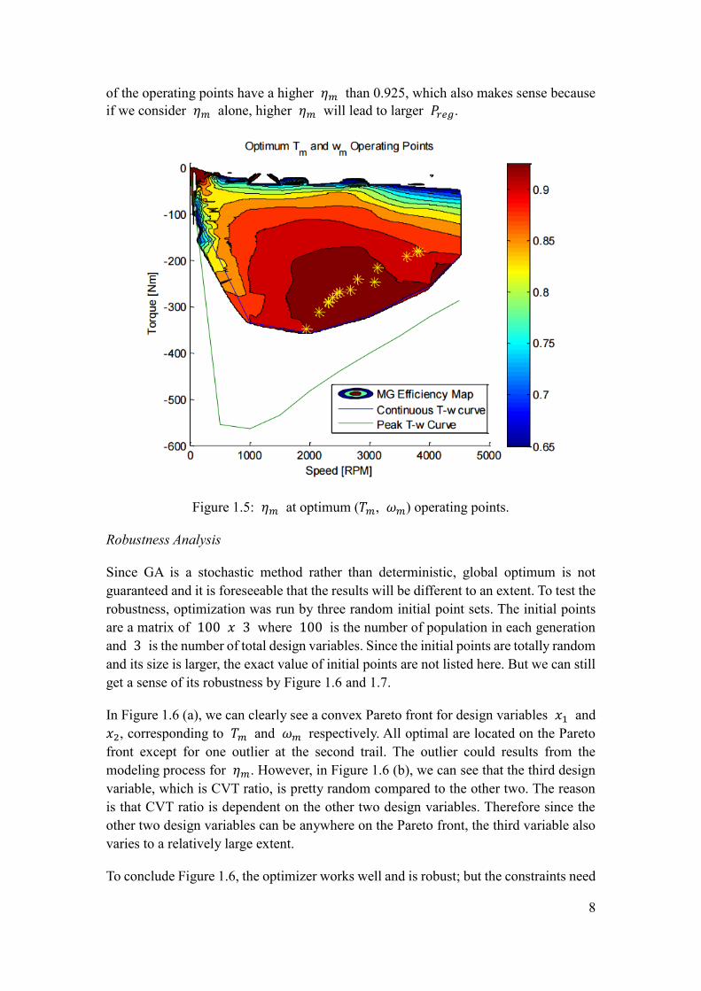
8

of the operating points have a higher 𝜂𝑚 than 0.925, which also makes sense because

if we consider 𝜂𝑚 alone, higher 𝜂𝑚 will lead to larger 𝑃𝑟𝑒𝑔.

Figure 1.5: 𝜂𝑚 at optimum (𝑇𝑚, 𝜔𝑚) operating points.

Robustness Analysis

Since GA is a stochastic method rather than deterministic, global optimum is not

guaranteed and it is foreseeable that the results will be different to an extent. To test the

robustness, optimization was run by three random initial point sets. The initial points

are a matrix of 100 𝑥 3 where 100 is the number of population in each generation

and 3 is the number of total design variables. Since the initial points are totally random

and its size is larger, the exact value of initial points are not listed here. But we can still

get a sense of its robustness by Figure 1.6 and 1.7.

In Figure 1.6 (a), we can clearly see a convex Pareto front for design variables 𝑥1 and

𝑥2, corresponding to 𝑇𝑚 and 𝜔𝑚 respectively. All optimal are located on the Pareto

front except for one outlier at the second trail. The outlier could results from the

modeling process for 𝜂𝑚. However, in Figure 1.6 (b), we can see that the third design

variable, which is CVT ratio, is pretty random compared to the other two. The reason

is that CVT ratio is dependent on the other two design variables. Therefore since the

other two design variables can be anywhere on the Pareto front, the third variable also

varies to a relatively large extent.

To conclude Figure 1.6, the optimizer works well and is robust; but the constraints need

9

to be defined better such that only one combination on the Pareto front is achieved.

(a)

(b)

Pareto Front

Outlier

10

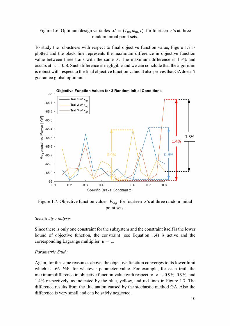
Figure 1.6: Optimum design variables 𝒙∗ = (𝑇𝑚, 𝜔𝑚, 𝑖) for fourteen 𝑧’s at three

random initial point sets.

To study the robustness with respect to final objective function value, Figure 1.7 is

plotted and the black line represents the maximum difference in objective function

value between three trails with the same 𝑧 . The maximum difference is 1.3 and

occurs at 𝑧 = 0.8. Such difference is negligible and we can conclude that the algorithm

is robust with respect to the final objective function value. It also proves that GA doesn’t

guarantee global optimum.

0.9%0.9%

1.4%1.3%

Figure 1.7: Objective function values 𝑃𝑟𝑒𝑔 for fourteen 𝑧’s at three random initial

point sets.

Sensitivity Analysis

Since there is only one constraint for the subsystem and the constraint itself is the lower

bound of objective function, the constraint (see Equation 1.4) is active and the

corresponding Lagrange multiplier 𝜇 = 1.

Parametric Study

Again, for the same reason as above, the objective function converges to its lower limit

which is -66 𝑘𝑊 for whatever parameter value. For example, for each trail, the

maximum difference in objective function value with respect to 𝑧 is 0.9 , 0.9 , and

1.4 respectively, as indicated by the blue, yellow, and red lines in Figure 1.7. The

difference results from the fluctuation caused by the stochastic method GA. Also the

difference is very small and can be safely neglected.

11

However, through our analysis, we found that the coupling variable 𝑇𝐷𝐵 is very

sensitive with regard to parameter value. So a parametric study is done on the coupling

variable. The results is summarized in Table 1.4 below.

Table 1.4: Summary of Parametric Study on Coupling Variable 𝑇𝐷𝐵

By varying each parameter value up and down by 30 of its original value, Table

1.4 shows that vehicle weight and tire radius are equally important and transmission

efficiency almost has no effect on coupling variable. As a result, if vehicle weight was

lower (equivalent to lower total braking torque demand) and tires were larger

(equivalent to larger braking torque moment arm), the minimum required torque on the

disk brake 𝑇𝐷𝐵, which is the coupling variable to the second subsystem, can be made

smaller.

12

Subsystem 2: Disc Braking System (Anqi Sun)

Background

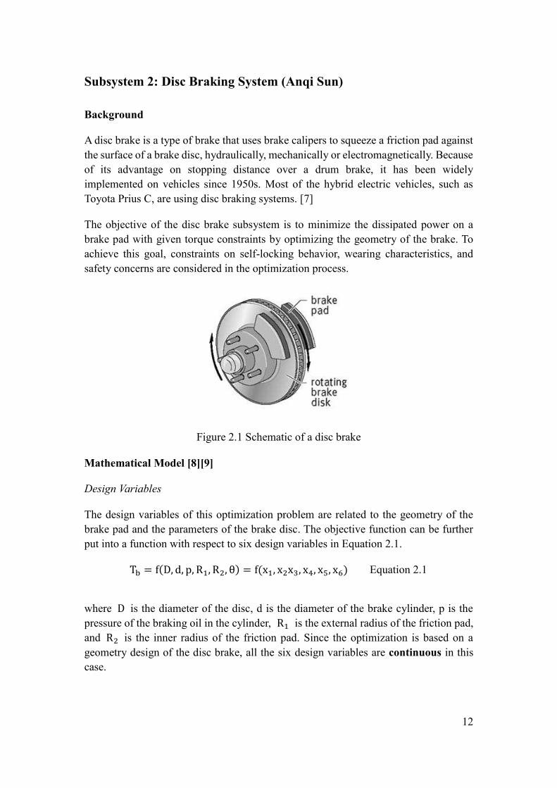
A disc brake is a type of brake that uses brake calipers to squeeze a friction pad against

the surface of a brake disc, hydraulically, mechanically or electromagnetically. Because

of its advantage on stopping distance over a drum brake, it has been widely

implemented on vehicles since 1950s. Most of the hybrid electric vehicles, such as

Toyota Prius C, are using disc braking systems. [7]

The objective of the disc brake subsystem is to minimize the dissipated power on a

brake pad with given torque constraints by optimizing the geometry of the brake. To

achieve this goal, constraints on self-locking behavior, wearing characteristics, and

safety concerns are considered in the optimization process.

Figure 2.1 Schematic of a disc brake

Mathematical Model [8][9]

Design Variables

The design variables of this optimization problem are related to the geometry of the

brake pad and the parameters of the brake disc. The objective function can be further

put into a function with respect to six design variables in Equation 2.1.

Tb = f(D, d, p, R1, R2, θ) = f(x1, x2x3, x4, x5, x6) Equation 2.1

where D is the diameter of the disc, d is the diameter of the brake cylinder, p is the

pressure of the braking oil in the cylinder, R1 is the external radius of the friction pad,

and R2 is the inner radius of the friction pad. Since the optimization is based on a

geometry design of the disc brake, all the six design variables are continuous in this

case.

13

Design variables of the friction pad is indicated in Figure 2.2.

Figure 2.2. Structural design variables of the friction pad. [8]

Design

Variables

Definition Design

Variables

Definition

D Diameter of brake pad R1 Outer radius of friction pad

d Diameter of brake

cylinder

R2 Inner radius of friction pad

p Pressure of braking oil θ Wrap angle of friction pad

Objective Function

The objective of the disc brake subsystem is to minimized the dissipated power on a

brake pad of the disc brake on a hybrid electric vehicle. The objective function is

𝑃𝐷𝐵 = (𝑅22 − 𝑅1

2)𝜃[𝑒]

Equation 2.2

where (𝑅22 − 𝑅1

2)𝜃 represents the friction area of the brake pad and [𝑒]=6𝑊/𝑚𝑚^2is

the upper limit of specific energy dissipation rate

Model Construction

The maximum torque constraint is derived from an analytic model that captures the

physics of the disc brake. q is the pressure that the friction plate exerted on the brake.

Therefore, the total braking torque on both sides is

Tb = 2 ∫ ∫ μqR2dRdθ =2

3μq(R2

3 − R13)θ

R2

R1

θ

2

−θ

2

Equation 2.3

14

According to the hydraulic rules, the unit pressure q is scaled from the pressure of oil

in the cylinder p, which is an inverse of the ratio of the action area. It can be

formulated as the inverse of

q =1

4πd2

1

2(R2

2−R12)θ

p =1

2πd2

(R22−R1

2)θp Equation 2.4

Substitute Equation 10 to Equation 9, we can conclude the objective function in

Equation 8. The design variable θ is canceled in the objective function.

Constraints

The optimization of the disc brake design is constrained by the following rules. All

constant parameters used in the model are listed in Table 2.1.

(1) Braking torque constraint: The requirement of the braking torque is determined

by the control logic of Regenerative Braking System. Based on different braking

conditions (z), the braking torque required from the mechanical disc brake

varies. For a subsystem level problem, TDBL = 2700Nm is used and a safety

factor of SF = 1.5 is multiplied to the limit.

2

3nμq(R2

3 − R13)θ ≥ TDBL ⋅ SF Equation 2.5

(2) Self-locking constraints: To avoid self-locking, the following constraint should

be satisfied:

μTf ≤1

2μLGβr

Equation

2.6

(3) Constraint of maximum pressure on the friction pad: This constraint is to

guarantee the lifetime of the disc brake.

β1Re

R1⋅

πd2

4A1p < [P]

Equation 2.7

Where β1 =4R1R2

(𝑅1+𝑅2)𝑅𝑒+2𝑅1𝑅2 , R𝑒 =

2

3(𝑅2

3−𝑅13)

𝑅22−𝑅1

2 , 𝐴1 =𝜃(𝑅2

2−𝑅12)

2

(4) Constraint of wearing characteristic

1

2⋅

mv12

2tA1≤

1

2μLGβr

Equation 2.8

15

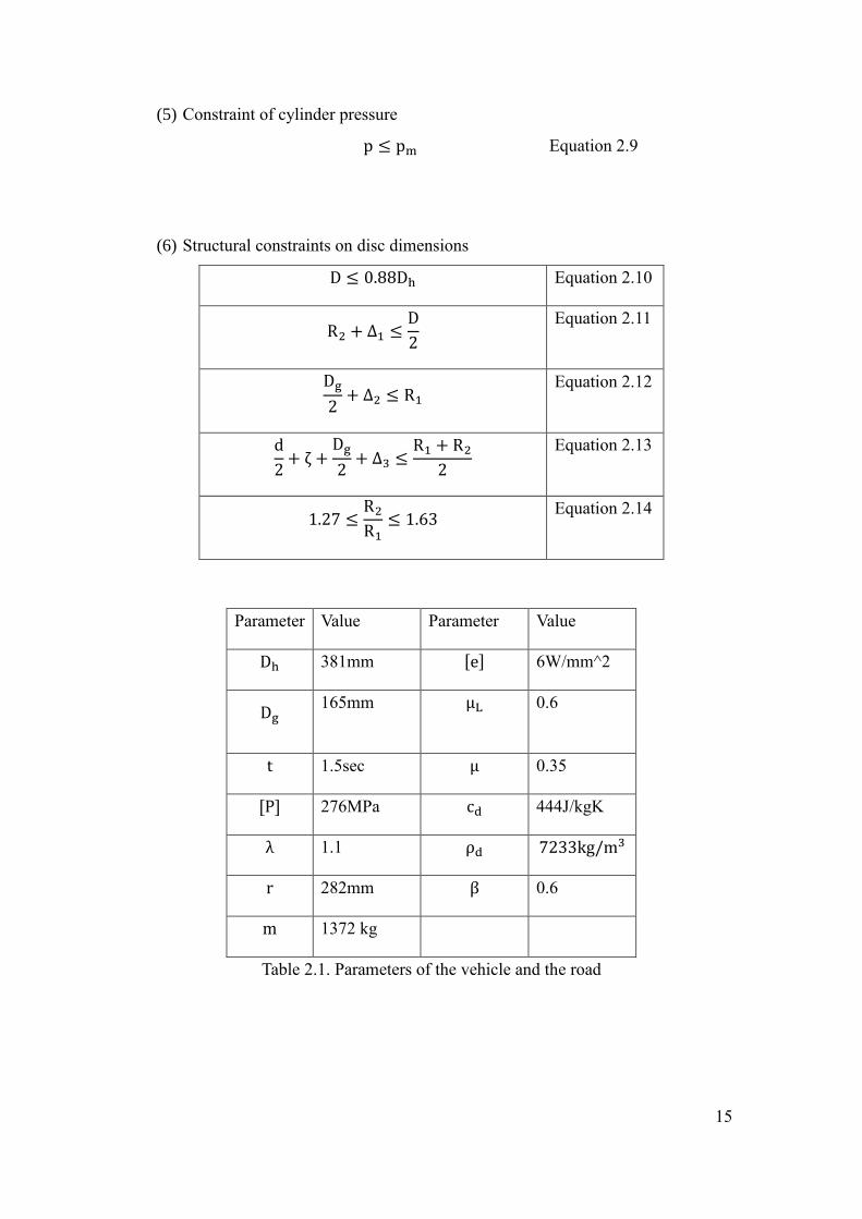
(5) Constraint of cylinder pressure

p ≤ pm Equation 2.9

(6) Structural constraints on disc dimensions

D ≤ 0.88Dh Equation 2.10

R2 + Δ1 ≤D

2

Equation 2.11

Dg

2+ Δ2 ≤ R1

Equation 2.12

d

2+ ζ +

Dg

2+ Δ3 ≤

R1 + R2

2

Equation 2.13

1.27 ≤R2

R1≤ 1.63

Equation 2.14

Parameter Value Parameter Value

Dh 381mm [e] 6W/mm^2

Dg 165mm μL 0.6

t 1.5sec μ 0.35

[P] 276MPa cd 444J/kgK

λ 1.1 ρd 7233kg/m3

r 282mm β 0.6

m 1372 kg

Table 2.1. Parameters of the vehicle and the road

16

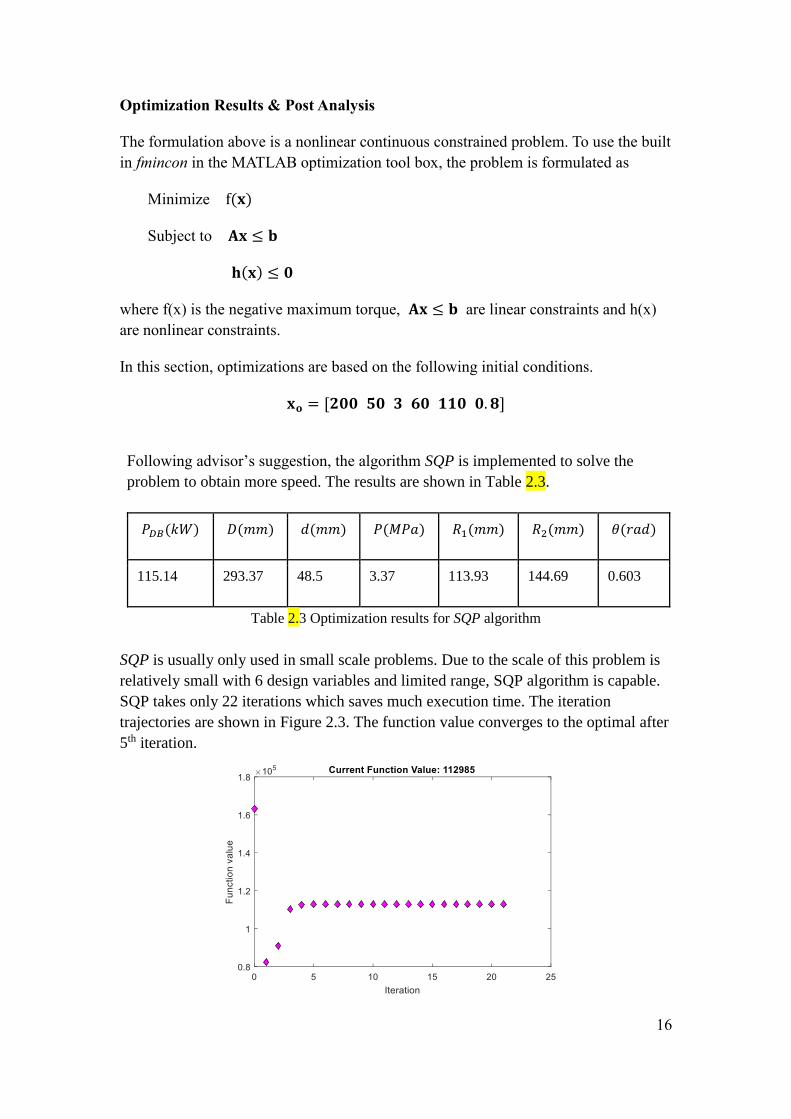
Optimization Results & Post Analysis

The formulation above is a nonlinear continuous constrained problem. To use the built

in fmincon in the MATLAB optimization tool box, the problem is formulated as

Minimize f(𝐱)

Subject to 𝐀𝐱 ≤ 𝐛

𝐡(𝐱) ≤ 𝟎

where f(x) is the negative maximum torque, 𝐀𝐱 ≤ 𝐛 are linear constraints and h(x)

are nonlinear constraints.

In this section, optimizations are based on the following initial conditions.

𝐱𝐨 = [𝟐𝟎𝟎 𝟓𝟎 𝟑 𝟔𝟎 𝟏𝟏𝟎 𝟎. 𝟖]

Following advisor’s suggestion, the algorithm SQP is implemented to solve the

problem to obtain more speed. The results are shown in Table 2.3.

𝑃𝐷𝐵(𝑘𝑊) 𝐷(𝑚𝑚) 𝑑(𝑚𝑚) 𝑃(𝑀𝑃𝑎) 𝑅1(𝑚𝑚) 𝑅2(𝑚𝑚) 𝜃(𝑟𝑎𝑑)

115.14 293.37 48.5 3.37 113.93 144.69 0.603

Table 2.3 Optimization results for SQP algorithm

SQP is usually only used in small scale problems. Due to the scale of this problem is

relatively small with 6 design variables and limited range, SQP algorithm is capable.

SQP takes only 22 iterations which saves much execution time. The iteration

trajectories are shown in Figure 2.3. The function value converges to the optimal after

5th iteration.

17

Figure 2.3. Function value converges with SQP

The minimum dissipated power on the brake pad is 112.98kW, corresponding to a friction

area of 18830𝑚𝑚2, which is similar to the existed brake pad design in the market.

Parametric Study of Lower Limit of Maximum Torque

As mentioned in previous section, the lower limit of maximum torque is an output of

the regenerative system. It is important to study the impact of the change in the lower

limit of maximum torque. The default value is 2750 Nm. By increasing and

decreasing the value by 10 , the corresponding objective function values are

evaluated in the following table. As indicated the table, the optimal dissipated power

changes by the same percentage as the required disc braking torque, which is

consistent with the analytical model. When more braking torque is required from the

disc brake, a larger brake pad area is needed, which leads to a larger dissipated power

on the brake pad.

Required Disc Braking Torque 𝑇𝐷𝐵𝐿

+10% -10%

Dissipated Power 𝑃𝐷𝐵(𝑊) 126.65 103.62

Δ𝑃𝐷𝐵 +10% -10%

Table 2.4 Parametric study of the required disc braking torque 𝑇𝐷𝐵𝐿

Sensitivity Analysis

The activities of all the eleven constraints are tested and shown in Table 2.5.

Constraints Activity Lagrange

Multipliers

2

3nμq(R2

3 − R13)θ ≥ TDBL ⋅ SF

Active 0.0279

μTf ≤1

2μLGβr

Non-active 0

β1Re

R1⋅

πd2

4A1p < [P]

Active 47434

1

2⋅

mv12

2tA1≤

1

2μLGβr

Non-active 0

p ≤ pm Non-active 0

18

D ≤ 0.88Dh Active 437.7

R2 + Δ1 ≤D

2

Non-active 0

Dg

2+ Δ2 ≤ R1

Non-active 0

d

2+ ζ +

Dg

2+ Δ3 ≤

R1 + R2

2

Active 875.4

1.27 ≤R2

R1

Active 91779

R2

R1≤ 1.63

Non-active 0

Table 2.5 Activity of all eleven constraints

(1) The sensitivity of the maximum torque constraint is equivalent to the parametric

study, which will not be elaborated in this section.

(2) If the maximum pressure on the brake pad constraint β1Re

R1⋅

πd2

4A1p < [P] is

released by altering [P] from 2.67MPa to 3MPa, the optimal objective function

value is reduced by 46.8 to 60.0kW. The objective function is sensitive to this

constraint.

(3) If one of the active structural constraint −R2

R1≤ −1.27 is released to

R2

R1≤

−1.1, the optimal objective function value is decreased by 24 to 84.9kW. The

objective function is sensitive to this constraint.

19

Whole System: Parallel Braking System

Background

Parallel regenerative braking system is an energy recovery system for hybrid electric

vehicles (HEVs) with combining effort of both conventional friction brake such as disk

brake in this project, and regenerative brake that converts kinetic energy into electric

energy for subsequent re-use.

The whole system is linked together through braking force. As seen from Figure 3.1

below, the braking force provided by disk braking, plus that from regenerative braking

should be equal to the total braking force required. With such connection, the two

subsystems are interactive and dependent on each other.

Figure 3.1: Connections between the overall system and two subsystems.

The goal of the integrated system is to minimize the braking power by specifying

generator operating condition (subsystem 1) and disk braking geometric sizing

(subsystem 2).

Mathematical Model

Coupling Variable

The system is divided into two subsystems using individual disciplinary feasible (IDF)

coordination method, as shown in Figure 3.2 below. The analyzer for each subsystem

is the objective function of each individual system as presented in the previous sections.

However, the coupling variable 𝑇𝐷𝐵 , which is the minimum braking torque

requirement for the disk brake in 𝑁𝑚, is the output of regenerative braking system and

do not require input from disk braking system. So the whole system is weakly coupled

and only 𝑦21 exists. Such characteristic make it easy for the integration and

computation process since fixed point iteration is not necessary.

20

Figure 3.2: IDF system coordination with 𝑦21 = 𝑇𝐷𝐵

Design Variables

There are nine design variables for the combined system, listed in Table 3.1 below. The

first three originate from subsystem 1, and the other six are from subsystem 2. The

definition, type, unit, and bounds are the same as they originally are in each subsystem.

Note that all design variables are local. Because the first two design variables are

discrete, the problem needs to be solved using GA.

Table 3.1: Design Variables for Combined System

Design

Variable Definition Type Unit

Upper and Lower

Bound

𝑇𝑚 Output torque of MG Discrete 𝑁𝑚 [0,600]

𝜔𝑚 Output speed of MG Discrete 𝑅𝑃𝑀 [0,5000]

𝑖 CVT ratio Continuous / [0.5,10]

𝐷 Diameter of the disk Continuous 𝑚𝑚 [200,300]

𝜃 Wrap angle of friction pad Continuous 𝑟𝑎𝑑 [0.1, 2.09]

𝑑 Diameter of brake cylinder Continuous 𝑚𝑚 [35,55]

𝑝 Pressure of braking oil Continuous 𝑀𝑃𝑎 [3,5]

𝑅1 Outer radius of friction pad Continuous 𝑚𝑚 [50,120]

𝑅2 Inner radius of friction pad Continuous 𝑚𝑚 [90,200]

21

Objective Function

The objective is to minimize the net power required by the parallel braking system. The

objective function is defined in Equation 3.1:

Min 𝑃𝑛𝑒𝑡 = 𝑃𝑅𝐵 + 𝑃𝐷𝐵 Equation 3.1

where 𝑃𝑛𝑒𝑡 is the net braking power, 𝑃𝑅𝐵 is the regenerative braking power (a

negative power provided by generator), and 𝑃𝐷𝐵 is the braking power required on the

disk brake pad. The units are all 𝑘𝑊.

The two items in Equation 3.1 are provided separately from the two analyzers.

Constraints

The constraints for the whole system is the combined set of constraints from the two

subsystems. There is one constraint from the regenerative braking system, specified in

Equation 1.4; there are six constraints from the disk braking system, as defined in

Equation 2.5 to 2.14.

As mentioned in previous section, the two subsystems, Regenerative Braking System

and Disc Braking System are weakly coupled, and they are linked by the required

braking torque from the disc braking system. Two system level optimization methods

are implemented to minimize the net power consumption of braking system.

System Level Optimization

As mentioned in previous section, the two subsystems, Regenerative Braking System

and Disc Braking System are weakly coupled, and they are linked by the required

braking torque from the disc braking system. Two system level optimization methods

are implemented to minimize the net power consumption of braking system.

(A) Individual Disciplinary Feasible (IDF)

Method

Since the two subsystems are weakly coupled, the first optimization method we

implemented is the individual disciplinary feasible method.

A set of design variables are assigned to the Regenerative Braking System by the

system level optimizer and the Regenerative Braking System executed with the given

variables and generated a maximum required torque 𝑇𝐷𝐵𝐿. Using the maximum

required torque from disc brake as an input of the Disc Braking System, the power

consumption in Disc Braking System 𝑃𝐷𝐵 is optimized. By combining the power

objective functions of the two subsystem, the minimized net power consumption of

braking system 𝑃𝑛𝑒𝑡 is generated by the system optimizer.

22

However, the randomness of GA leads to a fluctuation in 𝑇𝐷𝐵𝐿. Genetic Algorithm is

used in the Regenerative Braking System because of the discrete variables. Genetic

Algorithm applies mutations by generating some random cases following the given

scale and shrink. 𝑇𝐷𝐵𝐿 is quite sensitive to this change and the program cannot

generate identical 𝑇𝐷𝐵𝐿 in different runs with the same setting. To eliminate the

influence of the randomness, the Regenerative Braking optimization program was

executed for 30 times and the value of 𝑇𝐷𝐵𝐿 is plotted in the Figure 3.3.

Figure 3.3 𝑇𝐷𝐵𝐿 generated by GA in 30 iterations

The maximum value among the 30 results, 𝑇𝐷𝐵𝐿 = 2874.3 𝑁𝑚, is selected as the

lower limit for max braking torque in the Disc Braking System.

Results & Analysis

Using the algorithm stated above, the optimization results in shown in Table 3.2.

𝑃𝑛𝑒𝑡(𝑘𝑊) 𝑃𝐷𝐵(𝑘𝑊) 𝑃𝑅𝐵(𝑘𝑊) 𝑇𝐷𝐵𝐿(𝑁𝑚)

51.0 116.8 -65.8 2874.3

𝐷(𝑚𝑚) 𝑑(𝑚𝑚) 𝑃(𝑀𝑃𝑎) 𝑅1(𝑚𝑚) 𝑅2(𝑚𝑚) 𝜃(𝑟𝑎𝑑) 𝑇𝑚(𝑁𝑚) 𝜔𝑚[𝑅𝑃𝑀] i

293.37 51.42 2.86 113.01 144.68 0.596 310 2170 2.23

Table 3.2 Optimization result with IDF method

23

As indicated in Table 3.2, the minimum net power consumption of the braking system

is 51.0kW when z=0.8. The regenerative braking power is 65.8kW, which is

consistent with the Regenerative Braking System optimization result, though the

design variables varied because of the nature of GA and the problem definition, as

discussed in Robustness Analysis of Regenerative Braking System.

The disc braking power is 116.8kW in the system optimal condition, which is slightly

larger than the subsystem result. The deviation is reasonable because the value of

TDBL generated from the system optimizer is larger than the original setting in Disc

Braking System.

(B) 3.3.2 Multidisciplinary Feasible (MDF)

Method

In this case, the two subsystems are merged together and solved with the one

optimizer. Since there are discrete design variables in Regenerative Braking System,

SQP is not applicable to the overall optimization problem. Genetic algorithm is

implemented to solve the system level problem.

The initial population of the optimization problem is generated randomly between the

Upper Limit and Lower Limit of the system level problem with the following

equation.

𝐼𝑛𝑖𝑡𝑖𝑎𝑙 = 𝐿𝐵 + 𝑟𝑎𝑛𝑑(0,1) ⋅ (𝑈𝐵 − 𝐿𝐵) Equation 3.2

The design variables and the constraints of the two subsystem are directly combined

in this algorithm. The objective function is the net power consumption of the braking

system. There are 7 nonlinear constraints and 5 linear constraints in the system level

problem. The population size of the GA algorithm is 100 and the generation limitation

is 300.

The linking variable is implemented in the nonlinear constraint function. If the current

point is infeasible in the engine map, the algorithm will assign an infeasible large

value to the linking variable TDBL. Otherwise, the value of the linking variable is

assigned as TDBL = Td − Tm, where TD is the torque demand and Tm is the torque

from regenerative brake.

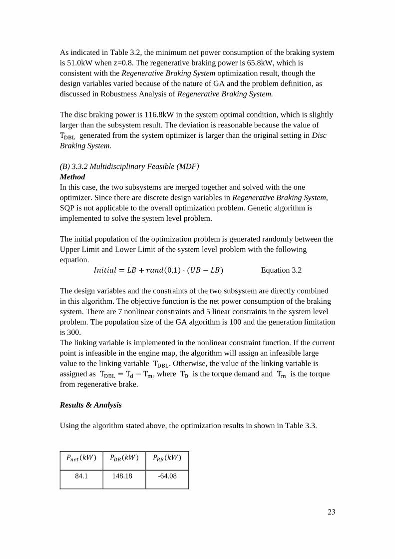
Results & Analysis

Using the algorithm stated above, the optimization results in shown in Table 3.3.

𝑃𝑛𝑒𝑡(𝑘𝑊) 𝑃𝐷𝐵(𝑘𝑊) 𝑃𝑅𝐵(𝑘𝑊)

84.1 148.18 -64.08

24

𝐷(𝑚𝑚) 𝑑(𝑚𝑚) 𝑃(𝑀𝑃𝑎) 𝑅1(𝑚𝑚) 𝑅2(𝑚𝑚) 𝜃(𝑟𝑎𝑑) 𝑇𝑚(𝑁𝑚) 𝜔𝑚[𝑅𝑃𝑀] i

261.12 48.86 3.84 94.88 122.46 1.03 222 2960 7.90

Table 3.3 Optimization result with MDF method

Figure 3.4 GA Convergence plot for the system level problem

As indicated in the figure, the GA algorithm converges rapidly at the first 40

generations and finally approaches the minimum within 300 generations (upper limit).

The minimum power consumption on the braking system is 84.1 kW with this

algorithm, which is much larger than the previous method, which indicates that the

GA algorithm failed to locate the global maximum of the system level problem.

The reason of the deviation is related to the nature of GA. It is hard to sufficiently

mutate and crossover an optimization problem with 9 design variables. In other word,

total number of 9 design variables will make the algorithm instable and inefficient,

which is not recommended by the team.

25

Reference

[1] Jingming, Z., Baoyu, S., & Xiaojing, N. (2008, September). Optimization of parallel

regenerative braking control strategy. In Vehicle Power and Propulsion Conference,

2008. VPPC'08. IEEE (pp. 1-4). IEEE.

[2] Wang, F., & Zhuo, B. (2008). Regenerative braking strategy for hybrid electric

vehicles based on regenerative torque optimization control. Proceedings of the

Institution of Mechanical Engineers, Part D: Journal of Automobile

Engineering, 222(4), 499-513.

[3] Cholula, S., Claudio, A., & Ruiz, J. (2005, September). Intelligent control of the

regenerative braking in an induction motor drive. In Electrical and Electronics

Engineering, 2005 2nd International Conference on (pp. 302-308). IEEE.

[4] Dong, P. E. N. G., Cheng-liang, Y. I. N., & ZHANG, J. W. (2005). An investigation

into regenerative braking control strategy for hybrid electric vehicle. Academic Journal of

Shanghai Jiaotong University.

[5] Kim, D., & Kim, H. (2006). Vehicle stability control with regenerative braking and

electronic brake force distribution for a four-wheel drive hybrid electric

vehicle. Proceedings of the Institution of Mechanical Engineers, Part D: Journal of

Automobile Engineering, 220(6), 683-693.

[6] Mi, C., Lin, H., & Zhang, Y. (2005). Iterative learning control of antilock braking

of electric and hybrid vehicles. Vehicular Technology, IEEE Transactions on, 54(2),

486-494.

[7] Atkins, T.; Escudier, M.(2013). disc brake. In A Dictionary of Mechanical

Engineering. : Oxford University Press. Retrieved 24 Jan. 2016, from

http://www.oxfordreference.com.proxy.lib.umich.edu/view/10.1093/acref/978019958

7438.001.0001/acref-9780199587438-e-1543.

[8] Li,Z. & Zhang, X. (2009). Optimal design for caliper disc brake. Machine Design

and Research, vol.25,no.2,83-85

[9] Zhang, Y., Zhang, H., & Lu, C. (2012). Study on Parameter Optimization Design

of Drum Brake Based on Hybrid Cellular Multiobjective Genetic

Algorithm. Mathematical Problems in Engineering, 2012.

[10] http://www.mathworks.com/help/optim/ug/when-the-solver-fails.html#br77x8v

26

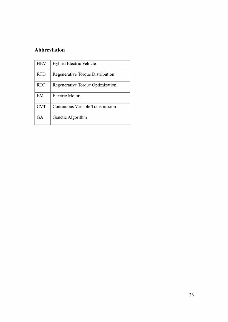
Abbreviation

HEV Hybrid Electric Vehicle

RTD Regenerative Torque Distribution

RTO Regenerative Torque Optimization

EM Electric Motor

CVT Continuous Variable Transmission

GA Genetic Algorithm