me590 report (2013 winter) - university of michiganyuqingz/report/me590_2013w.pdf · me590 report...

ME590 Report (2013 winter)

Renewable Energy (Solar/Wind Power) Supply Model

An Application of SAM Simulation Core (SSC) Software Development Kit (SDK)

Yuqing Zhou

Algorithmic Synthesis Laboratory (ASL)

Department of Mechanical Engineering

University of Michigan

April 2013

1

Contents

Abstract ......................................................................................................................................................... 2

1. Introduction to SAM Simulation Core (SSC) Software Development Kit (SDK) .... 2

2. Introduction to Solar/Wind Power System .......................................................................... 2

2.1 Solar Power Supply System ........................................................................................................... 2

2.2 Wind Power Supply System .......................................................................................................... 3

3. Module Database ............................................................................................................................ 4

3.1 Solar PV Module ............................................................................................................................ 4

3.2 Solar Inverter Module ................................................................................................................... 5

3.3 Wind Turbine Module ................................................................................................................... 6

4. Model Function ................................................................................................................................ 6

4.1 PV/Inverter/Turbine Module Reader Function (‘pvrader’, ‘invreader’, ‘tbreader’) ................... 6

4.2 Solar/Wind Energy Supply Function (‘solarpwr’, ‘windpwr’) ..................................................... 7

4.3 System Main Function (‘mainsolar’, ‘mainwind’) ...................................................................... 11

5. Result Analysis ................................................................................................................................ 12

5.1 Solar Energy Model Test Result .................................................................................................. 12

5.2 Wind Energy Model Test Result .................................................................................................. 14

6. Conclusion ........................................................................................................................................ 15

Reference ................................................................................................................................................... 16

2

Abstract

By using NREL recently released SAM Simulation Core (SSC) Software

Development Kit (SDK) in MATLAB environment, we made the analytical and

mathematical models of the energy supply capacity of distributed renewable

energy sources including solar and wind power. The module database for PV,

inverter and wind turbine is also established in order to reduce the module spec

inputs to the main function. Compared with System Advisor Model (SAM)

software, there is less than 1.0% error between our model and SAM.

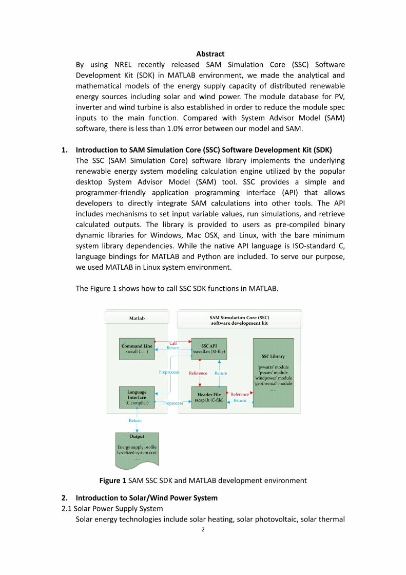
1. Introduction to SAM Simulation Core (SSC) Software Development Kit (SDK)

The SSC (SAM Simulation Core) software library implements the underlying

renewable energy system modeling calculation engine utilized by the popular

desktop System Advisor Model (SAM) tool. SSC provides a simple and

programmer-friendly application programming interface (API) that allows

developers to directly integrate SAM calculations into other tools. The API

includes mechanisms to set input variable values, run simulations, and retrieve

calculated outputs. The library is provided to users as pre-compiled binary

dynamic libraries for Windows, Mac OSX, and Linux, with the bare minimum

system library dependencies. While the native API language is ISO-standard C,

language bindings for MATLAB and Python are included. To serve our purpose,

we used MATLAB in Linux system environment.

The Figure 1 shows how to call SSC SDK functions in MATLAB.

Figure 1 SAM SSC SDK and MATLAB development environment

2. Introduction to Solar/Wind Power System

2.1 Solar Power Supply System

Solar energy technologies include solar heating, solar photovoltaic, solar thermal

3

electricity, solar architecture and artificial photosynthesis. The technology we

are interested in is the solar photovoltaic which converts sunlight into electric

current using the photoelectric effect.

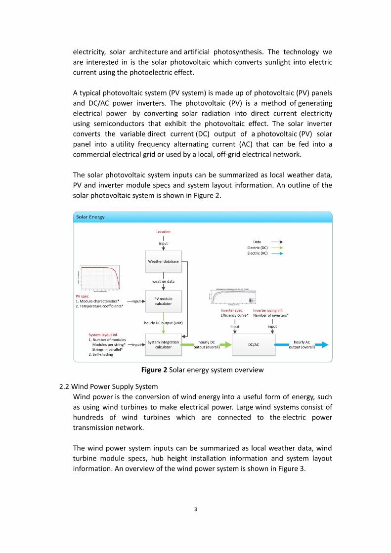
A typical photovoltaic system (PV system) is made up of photovoltaic (PV) panels

and DC/AC power inverters. The photovoltaic (PV) is a method of generating

electrical power by converting solar radiation into direct current electricity

using semiconductors that exhibit the photovoltaic effect. The solar inverter

converts the variable direct current (DC) output of a photovoltaic (PV) solar

panel into a utility frequency alternating current (AC) that can be fed into a

commercial electrical grid or used by a local, off-grid electrical network.

The solar photovoltaic system inputs can be summarized as local weather data,

PV and inverter module specs and system layout information. An outline of the

solar photovoltaic system is shown in Figure 2.

Figure 2 Solar energy system overview

2.2 Wind Power Supply System

Wind power is the conversion of wind energy into a useful form of energy, such

as using wind turbines to make electrical power. Large wind systems consist of

hundreds of wind turbines which are connected to the electric power

transmission network.

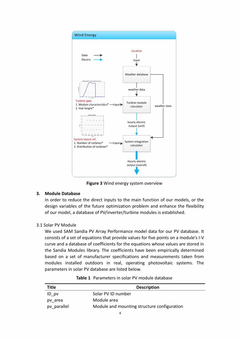
The wind power system inputs can be summarized as local weather data, wind

turbine module specs, hub height installation information and system layout

information. An overview of the wind power system is shown in Figure 3.

4

Figure 3 Wind energy system overview

3. Module Database

In order to reduce the direct inputs to the main function of our models, or the

design variables of the future optimization problem and enhance the flexibility

of our model, a database of PV/inverter/turbine modules is established.

3.1 Solar PV Module

We used SAM Sandia PV Array Performance model data for our PV database. It

consists of a set of equations that provide values for five points on a module’s I-V

curve and a database of coefficients for the equations whose values are stored in

the Sandia Modules library. The coefficients have been empirically determined

based on a set of manufacturer specifications and measurements taken from

modules installed outdoors in real, operating photovoltaic systems. The

parameters in solar PV database are listed below.

Table 1 Parameters in solar PV module database

Title Description

ID_pv Solar PV ID number

pv_area Module area

pv_parallel Module and mounting structure configuration

5

3.2 Solar Inverter Module

We used the Sandia Performance Model for Grid-Connected PV Inverters from a

database of commercially available inverters maintained by Sandia National

Laboratory as our inverter spec data.

The Sandia model consists of a set of equations that SAM uses to calculate the

pv_A Temperature coefficient a

pv_B Temperature coefficient b

pv_DTC Temperature coefficient dT

pv_FD Diffuse fraction

pv_A0 Air mass polynomial coeff 0





pv_aimp Max power point current temperature coefficient

pv_aisc Short circuit current temperature coefficient

pv_B0 Incidence angle modifier polynomial coeff 0






pv_bvmpo Max power point voltage temperature coefficient

pv_bvoco Open circuit voltage temperature coefficient

pv_c0 C0

pv_c1 C1

pv_c2 C2

pv_c3 C3

pv_c4 C4

pv_c5 C5

pv_c6 C6

pv_c7 C7

pv_impo Max power point current

pv_isco Short circuit current

pv_ixo Ix midpoint current

pv_ixxo Ixx midpoint current

pv_mbvmp Irradiance dependence of Vmp temperature coefficient

pv_mbvoc Irradiance dependence of Voc temperature coefficient

pv_n Diode factor

pv_series Number of cells in series

pv_vmpo Max power point voltage

pv_voco Open circuit voltage

6

inverter's hourly AC output based on the DC input and a set of

empirically-determined coefficients that describe the inverter's performance

characteristics. The equations involve a set of coefficients that have been

empirically determined based on data from manufacturer specification sheets

and either field measurements from inverters installed in operating systems, or

laboratory measurements using the California Energy Commission (CEC) test

protocol. The parameters in inverter database are listed below.

Table 2 Parameters in inverter module database

Title Description

ID_inv Inverter ID number

inv_c0 Curvature between ac-power and dc-power at ref

inv_c1 Coefficient of Pdco variation with dc input voltage

inv_c2 Coefficient of Pso variation with dc input voltage

inv_c3 Coefficient of Co variation with dc input voltage

inv_paco AC maximum power rating

inv_pdco DC input power at which ac-power rating is achieved

inv_pnt AC power consumed by inverter at night

inv_pso DC power required to enable the inversion process

inv_vdco DC input voltage for the rated ac-power rating

inv_vdcmax Maximum dc input operating voltage

3.3 Wind Turbine Module

We used SAM turbine spec data to establish the wind turbine database.

According to the database, it can automatically populate the power curve, rated

output and rotor diameter values. The parameters in wind turbine database are

listed below.

Table 3 Parameters in wind turbine module database

Title Description

ID_tb Wind turbine ID number

hub_efficiency Turbulence coefficient

pc_wind Power curve wind speed array

pc_power Power curve turbine output array

rotor_di Rotor diameter

cut_in Cut-in wind speed

4. Model Function

4.1 PV/Inverter/Turbine Module Reader Function (‘pvrader’, ‘invreader’, ‘tbreader’)

With the input of PV/inverter/turbine module ID number, the certain reader

function will return the PV/inverter/turbine module spec parameters listed in

Table1 to 3 to the workspace for later usage of solar/wind energy performance

function.

7

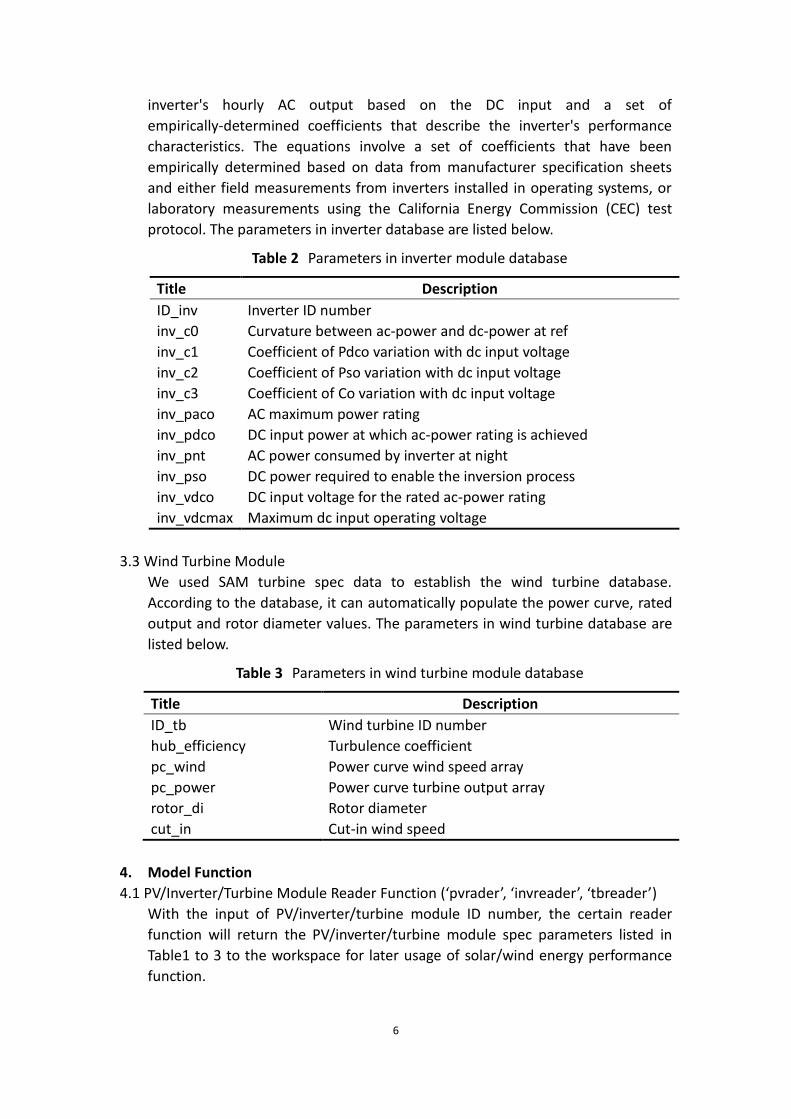
The function content for ‘invreader’ is listed below. In addition, the ‘pvreader’

and ‘tbreader’ functions have the similar function contents as the one listed.

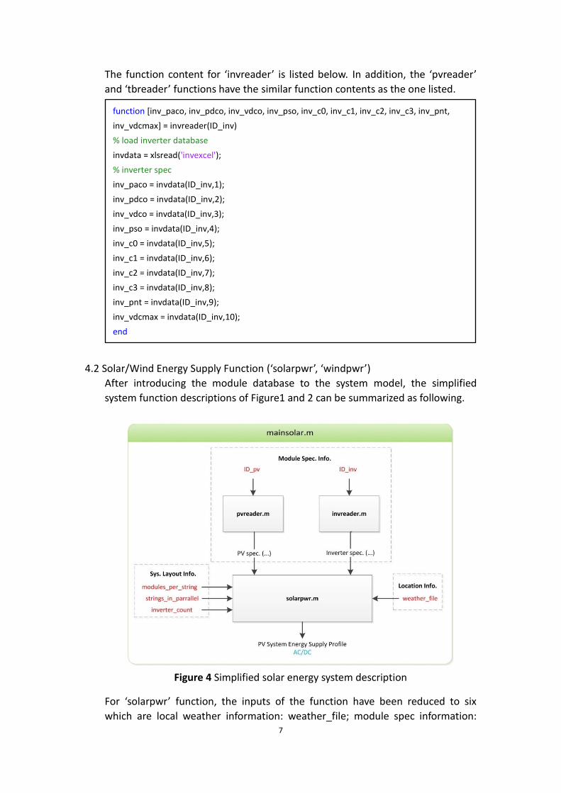
4.2 Solar/Wind Energy Supply Function (‘solarpwr’, ‘windpwr’)

After introducing the module database to the system model, the simplified

system function descriptions of Figure1 and 2 can be summarized as following.

Figure 4 Simplified solar energy system description

For ‘solarpwr’ function, the inputs of the function have been reduced to six

which are local weather information: weather_file; module spec information:

function [inv_paco, inv_pdco, inv_vdco, inv_pso, inv_c0, inv_c1, inv_c2, inv_c3, inv_pnt,

inv_vdcmax] = invreader(ID_inv)

% load inverter database

invdata = xlsread('invexcel');

% inverter spec

inv_paco = invdata(ID_inv,1);

inv_pdco = invdata(ID_inv,2);

inv_vdco = invdata(ID_inv,3);

inv_pso = invdata(ID_inv,4);

inv_c0 = invdata(ID_inv,5);




inv_pnt = invdata(ID_inv,9);

inv_vdcmax = invdata(ID_inv,10);

end

8

ID_pv, ID_inv; system layout information: modules_per_string,

strings_in_parrallel, inverter_count. Running the function, the output of hourly

AC or DC solar energy profile can be obtained.

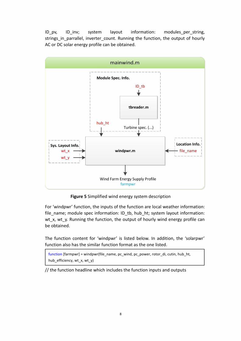
Figure 5 Simplified wind energy system description

For ‘windpwr’ function, the inputs of the function are local weather information:

file_name; module spec information: ID_tb, hub_ht; system layout information:

wt_x, wt_y. Running the function, the output of hourly wind energy profile can

be obtained.

The function content for ‘windpwr’ is listed below. In addition, the ‘solarpwr’

function also has the similar function format as the one listed.

// the function headline which includes the function inputs and outputs

function [farmpwr] = windpwr(file_name, pc_wind, pc_power, rotor_di, cutin, hub_ht,

hub_efficiency, wt_x, wt_y)

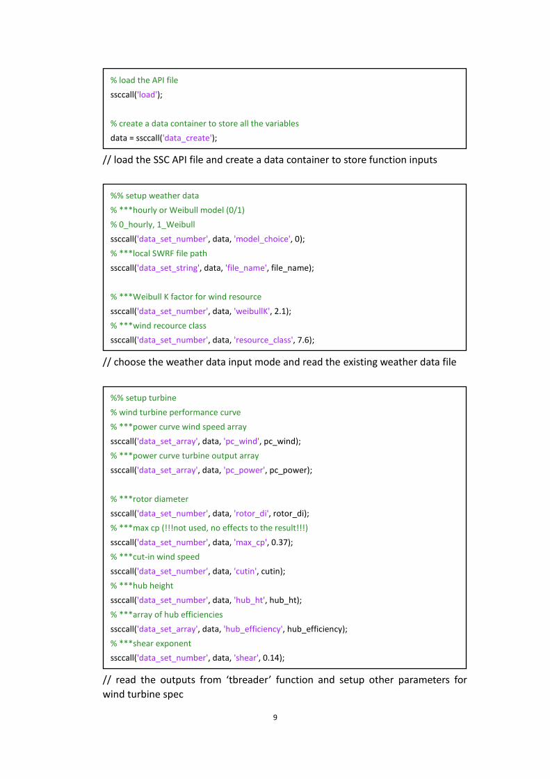
9

// load the SSC API file and create a data container to store function inputs

// choose the weather data input mode and read the existing weather data file

// read the outputs from ‘tbreader’ function and setup other parameters for

wind turbine spec

%% setup turbine

% wind turbine performance curve

% ***power curve wind speed array

ssccall('data_set_array', data, 'pc_wind', pc_wind);

% ***power curve turbine output array

ssccall('data_set_array', data, 'pc_power', pc_power);

% ***rotor diameter

ssccall('data_set_number', data, 'rotor_di', rotor_di);

% ***max cp (!!!not used, no effects to the result!!!)

ssccall('data_set_number', data, 'max_cp', 0.37);

% ***cut-in wind speed

ssccall('data_set_number', data, 'cutin', cutin);

% ***hub height

ssccall('data_set_number', data, 'hub_ht', hub_ht);

% ***array of hub efficiencies

ssccall('data_set_array', data, 'hub_efficiency', hub_efficiency);

% ***shear exponent

ssccall('data_set_number', data, 'shear', 0.14);

%% setup weather data

% ***hourly or Weibull model (0/1)

% 0_hourly, 1_Weibull

ssccall('data_set_number', data, 'model_choice', 0);

% ***local SWRF file path

ssccall('data_set_string', data, 'file_name', file_name);

% ***Weibull K factor for wind resource

ssccall('data_set_number', data, 'weibullK', 2.1);

% ***wind recource class

ssccall('data_set_number', data, 'resource_class', 7.6);

% load the API file

ssccall('load');

% create a data container to store all the variables

data = ssccall('data_create');

10

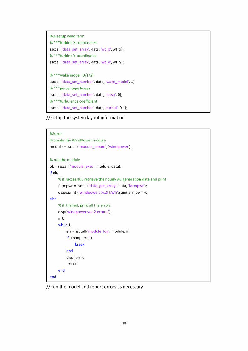
// setup the system layout information

// run the model and report errors as necessary

%% run

% create the WindPower module

module = ssccall('module_create', 'windpower');

% run the module

ok = ssccall('module_exec', module, data);

if ok,

% if successful, retrieve the hourly AC generation data and print

farmpwr = ssccall('data_get_array', data, 'farmpwr');

disp(sprintf('windpower: %.2f kWh',sum(farmpwr)));

else

% if it failed, print all the errors

disp('windpower ver.2 errors:');

ii=0;

while 1,

err = ssccall('module_log', module, ii);

if strcmp(err,''),

break;

end

disp( err );

ii=ii+1;

end

end

%% setup wind farm

% ***turbine X coordinates

ssccall('data_set_array', data, 'wt_x', wt_x);

% ***turbine Y coordinates

ssccall('data_set_array', data, 'wt_y', wt_y);

% ***wake model (0/1/2)

ssccall('data_set_number', data, 'wake_model', 1);

% ***percentage losses

ssccall('data_set_number', data, 'lossp', 0);

% ***turbulence coefficient

ssccall('data_set_number', data, 'turbul', 0.1);

11

// free the model, release the data container and unload the SAM library

4.3 System Main Function (‘mainsolar’, ‘mainwind’)

The main script for running the solar (wind) energy system model including

‘pvreader’, ‘invreader’ and ‘solarpwr’ (‘tbreader’ and ‘windpwr’) has been coded.

The format of the main script follows the flowchart in Figure 4 and 5.

The content of ‘mainsolar’ has been listed below which is similar to that of

‘mainwind’.

// read the weather file

// define the PV module ID and run ‘pvreader’ function which will return PV spec

information to the main script

// define the inverter module ID and run ‘invreader’ function which will return

inverter spec information to the main script

% define inverter spec (input: ID_inv)

ID_inv = 285;

[inv_paco, inv_pdco, inv_vdco, inv_pso, inv_c0, inv_c1, inv_c2, inv_c3, inv_pnt, inv_vdcmax]

= invreader(ID_inv);

% define PV spec (input: ID_pv)

ID_pv = 48;

[pv_area, pv_series, pv_parallel, pv_isco, pv_voco, pv_impo, pv_vmpo, pv_aisc, pv_aimp,

pv_c0, pv_c1, pv_bvoco, pv_mbvoc, pv_bvmpo, pv_mbvmp, pv_n, pv_c2, pv_c3, pv_A0,

pv_A1, pv_A2, pv_A3, pv_A4, pv_B0, pv_B1, pv_B2, pv_B3, pv_B4, pv_B5, pv_DTC, pv_FD,

pv_A, pv_B, pv_c4, pv_c5, pv_ixo, pv_ixxo, pv_c6, pv_c7] = pvreader(ID_pv);

%% setup input

% define weather location: Nagoya, Japan

weather_file = '/afs/umich.edu/user/y/u/yuqingz/Software/weatherdata/Solar_Nagoya.csv';

% free the PVWatts module that we created

ssccall('module_free', module);

% release the data container and all of its variables

ssccall('data_free', data);

% unload the library

ssccall('unload');

end

12

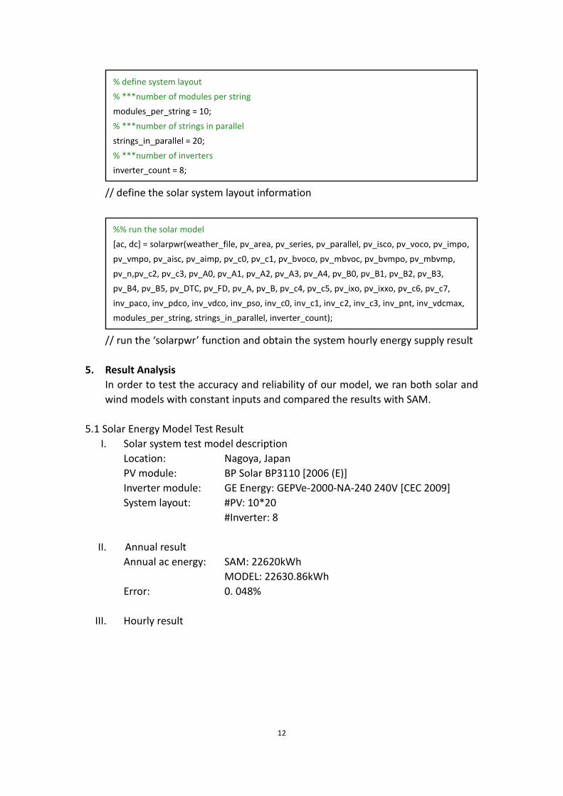
// define the solar system layout information

// run the ‘solarpwr’ function and obtain the system hourly energy supply result

5. Result Analysis

In order to test the accuracy and reliability of our model, we ran both solar and

wind models with constant inputs and compared the results with SAM.

5.1 Solar Energy Model Test Result

I. Solar system test model description

Location: Nagoya, Japan

PV module: BP Solar BP3110 [2006 (E)]

Inverter module: GE Energy: GEPVe-2000-NA-240 240V [CEC 2009]

System layout: #PV: 10*20

#Inverter: 8

II. Annual result

Annual ac energy: SAM: 22620kWh

MODEL: 22630.86kWh

Error: 0. 048%

III. Hourly result

%% run the solar model

[ac, dc] = solarpwr(weather_file, pv_area, pv_series, pv_parallel, pv_isco, pv_voco, pv_impo,

pv_vmpo, pv_aisc, pv_aimp, pv_c0, pv_c1, pv_bvoco, pv_mbvoc, pv_bvmpo, pv_mbvmp,

pv_n,pv_c2, pv_c3, pv_A0, pv_A1, pv_A2, pv_A3, pv_A4, pv_B0, pv_B1, pv_B2, pv_B3,

pv_B4, pv_B5, pv_DTC, pv_FD, pv_A, pv_B, pv_c4, pv_c5, pv_ixo, pv_ixxo, pv_c6, pv_c7,

inv_paco, inv_pdco, inv_vdco, inv_pso, inv_c0, inv_c1, inv_c2, inv_c3, inv_pnt, inv_vdcmax,

modules_per_string, strings_in_parallel, inverter_count);

% define system layout

% ***number of modules per string

modules_per_string = 10;

% ***number of strings in parallel

strings_in_parallel = 20;

% ***number of inverters

inverter_count = 8;

13

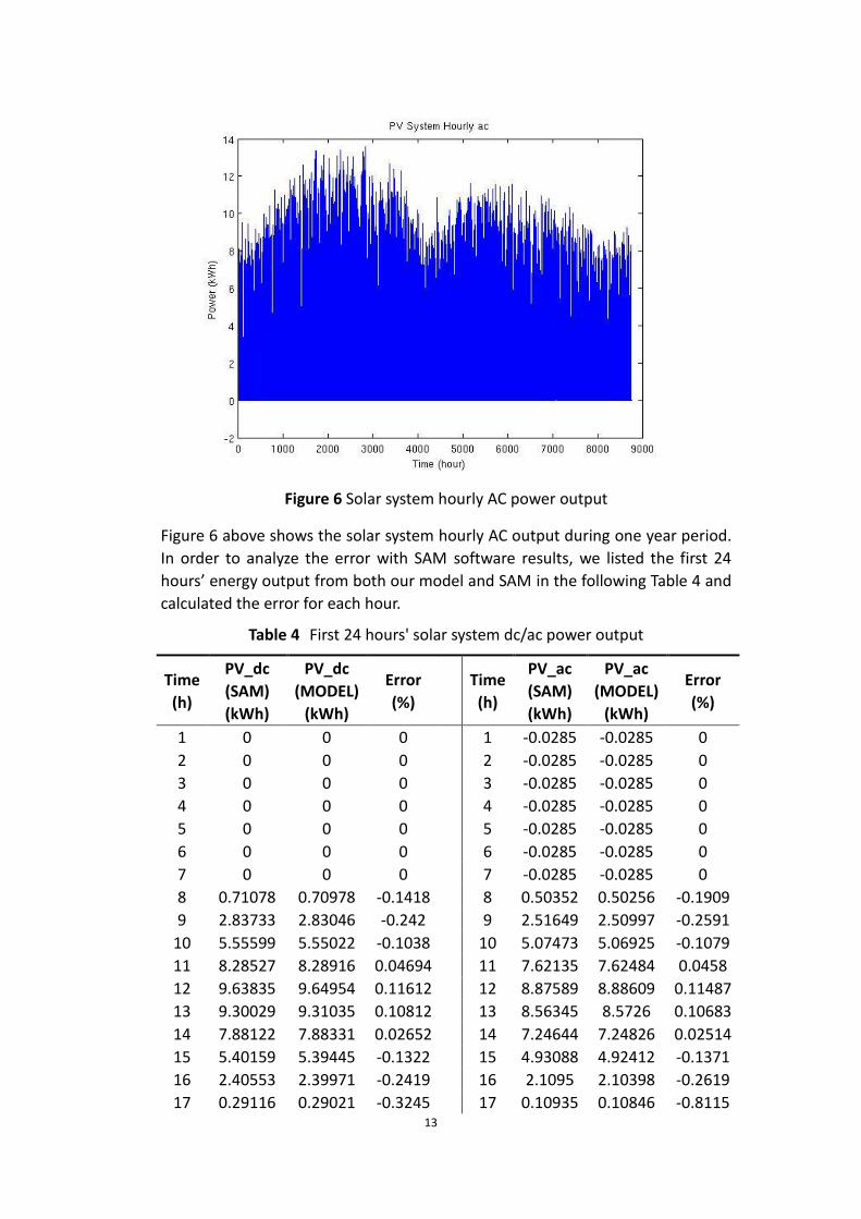
Figure 6 Solar system hourly AC power output

Figure 6 above shows the solar system hourly AC output during one year period.

In order to analyze the error with SAM software results, we listed the first 24

hours’ energy output from both our model and SAM in the following Table 4 and

calculated the error for each hour.

Table 4 First 24 hours' solar system dc/ac power output

Time

(h)

PV_dc

(SAM)

(kWh)

PV_dc

(MODEL)

(kWh)

Error

(%)

Time

(h)

PV_ac

(SAM)

(kWh)

PV_ac

(MODEL)

(kWh)

Error

(%)

1 0 0 0 1 -0.0285 -0.0285 0

2 0 0 0 2 -0.0285 -0.0285 0

3 0 0 0 3 -0.0285 -0.0285 0

4 0 0 0 4 -0.0285 -0.0285 0

5 0 0 0 5 -0.0285 -0.0285 0

6 0 0 0 6 -0.0285 -0.0285 0

7 0 0 0 7 -0.0285 -0.0285 0

8 0.71078 0.70978 -0.1418 8 0.50352 0.50256 -0.1909

9 2.83733 2.83046 -0.242 9 2.51649 2.50997 -0.2591

10 5.55599 5.55022 -0.1038 10 5.07473 5.06925 -0.1079

11 8.28527 8.28916 0.04694 11 7.62135 7.62484 0.0458

12 9.63835 9.64954 0.11612 12 8.87589 8.88609 0.11487

13 9.30029 9.31035 0.10812 13 8.56345 8.5726 0.10683

14 7.88122 7.88331 0.02652 14 7.24644 7.24826 0.02514

15 5.40159 5.39445 -0.1322 15 4.93088 4.92412 -0.1371

16 2.40553 2.39971 -0.2419 16 2.1095 2.10398 -0.2619

17 0.29116 0.29021 -0.3245 17 0.10935 0.10846 -0.8115

14

18 0 0 0 18 -0.0285 -0.0285 0

19 0 0 0 19 -0.0285 -0.0285 0

20 0 0 0 20 -0.0285 -0.0285 0

21 0 0 0 21 -0.0285 -0.0285 0

22 0 0 0 22 -0.0285 -0.0285 0

23 0 0 0 23 -0.0285 -0.0285 0

24 0 0 0 24 -0.0285 -0.0285 0

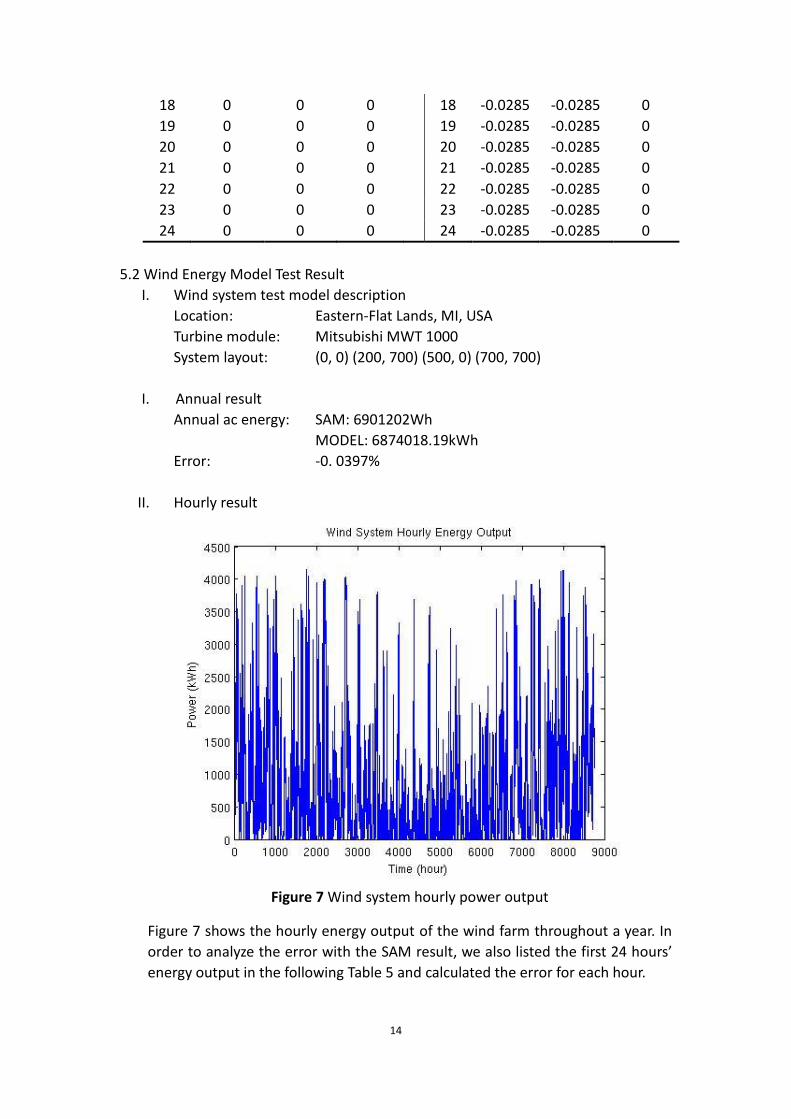
5.2 Wind Energy Model Test Result

I. Wind system test model description

Location: Eastern-Flat Lands, MI, USA

Turbine module: Mitsubishi MWT 1000

System layout: (0, 0) (200, 700) (500, 0) (700, 700)

I. Annual result

Annual ac energy: SAM: 6901202Wh

MODEL: 6874018.19kWh

Error: -0. 0397%

II. Hourly result

Figure 7 Wind system hourly power output

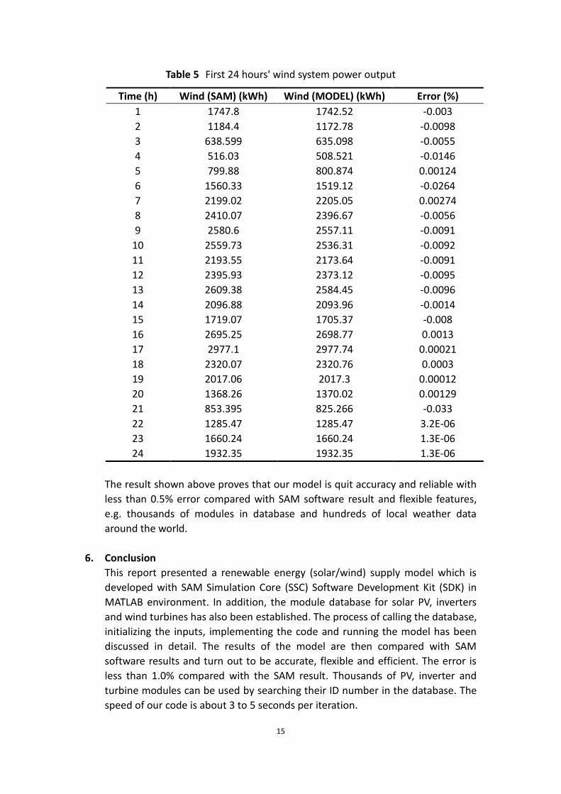
Figure 7 shows the hourly energy output of the wind farm throughout a year. In

order to analyze the error with the SAM result, we also listed the first 24 hours’

energy output in the following Table 5 and calculated the error for each hour.

15

Table 5 First 24 hours' wind system power output

Time (h) Wind (SAM) (kWh) Wind (MODEL) (kWh) Error (%)

1 1747.8 1742.52 -0.003

2 1184.4 1172.78 -0.0098

3 638.599 635.098 -0.0055

4 516.03 508.521 -0.0146

5 799.88 800.874 0.00124

6 1560.33 1519.12 -0.0264

7 2199.02 2205.05 0.00274

8 2410.07 2396.67 -0.0056

9 2580.6 2557.11 -0.0091

10 2559.73 2536.31 -0.0092

11 2193.55 2173.64 -0.0091

12 2395.93 2373.12 -0.0095

13 2609.38 2584.45 -0.0096

14 2096.88 2093.96 -0.0014

15 1719.07 1705.37 -0.008

16 2695.25 2698.77 0.0013

17 2977.1 2977.74 0.00021

18 2320.07 2320.76 0.0003

19 2017.06 2017.3 0.00012

20 1368.26 1370.02 0.00129

21 853.395 825.266 -0.033

22 1285.47 1285.47 3.2E-06

23 1660.24 1660.24 1.3E-06

24 1932.35 1932.35 1.3E-06

The result shown above proves that our model is quit accuracy and reliable with

less than 0.5% error compared with SAM software result and flexible features,

e.g. thousands of modules in database and hundreds of local weather data

around the world.

6. Conclusion

This report presented a renewable energy (solar/wind) supply model which is

developed with SAM Simulation Core (SSC) Software Development Kit (SDK) in

MATLAB environment. In addition, the module database for solar PV, inverters

and wind turbines has also been established. The process of calling the database,

initializing the inputs, implementing the code and running the model has been

discussed in detail. The results of the model are then compared with SAM

software results and turn out to be accurate, flexible and efficient. The error is

less than 1.0% compared with the SAM result. Thousands of PV, inverter and

turbine modules can be used by searching their ID number in the database. The

speed of our code is about 3 to 5 seconds per iteration.

16

Reference

[1] System Advisor Model Version 2013.1.15 (SAM 2013.1.15) National Renewable

Energy Laboratory. Golden, CO. https://sam.nrel.gov/content/downloads.

[2] System Advisor Model Version 2013.1.15 (SAM 2013.1.15) User Documentation.

National Renewable Energy Laboratory. Golden, CO.

me590 report (2013 winter) - university of michiganyuqingz/report/me590_2013w.pdf · me590 report...

Documents