mean field games on networks - uniroma1.it · mean field games on networks claudio marchi ......

Mean Field Games on networks

Claudio Marchi

Università di Padova

joint works with: S. Cacace (Rome) and F. Camilli (Rome)

C. Marchi (Univ. of Padova) Mean Field Games on networks Roma, June 14th, 2017 1 / 35

Outline

Brief introduction

Definition of networks

Formal derivation of the MFG system on networks

Study of the MFG system on networks

A numerical scheme

Model example on the torus Tn [Lasry-Lions,’06]

Consider a game with N rational and indistinguishable players. Thei-th player’s dynamics is

dX it = −αi

tdt +√

2νdW it , X i

0 = x i ∈ Tn

where ν > 0, W i are independent Brownian motions and αi is thecontrol chosen so to minimize the cost functional

lim infT→+∞

L(X is, α

is) + V

1N − 1

∑j 6=i

δX js

The Nash equilibria are characterized by a system of 2N equations. AsN → +∞, this system reduces to the following one:

(MFG-Tn)

−ν∆u + H(x ,Du) + ρ = V ([m]) in Tn

ν∆m + div(

m ∂H∂p (x ,Du)

)= 0 in Tn∫

Tn m dx = 1, m > 0∫Tn u dx = 0

H(x ,p) := supq∈Rn{−p · q − L(x ,q)};“[m]” means that V depends on m in a local or in a nonlocal way.

Theorem [Lasry-Lions ’06]There exists a smooth solution (u,m, ρ) to the above problem;Assume

I either V is strictly monotone in m (i.e.∫Tn (V ([m1])− V ([m2])) (m1 −m2)dx ≤ 0 implies m1 = m2)

I or V is monotone in m (i.e.∫Tn (V ([m1])− V ([m2]))(m1 −m2)dx≥0)

and H is strictly convex in p.

Then the solution is unique.

Basic References for MFG theory:Lasry-Lions, C.R. Math. Acad. Sci. Paris 343 (2006), 619-625.Lasry-Lions, C.R. Math. Acad. Sci. Paris 343 (2006), 679-684.Lasry-Lions, Jpn. J. Math. 2 (2007), 229-260.Huang-Malhamé-Caines, Commun. Inf. Syst. 6 (2006), 221-251.Lions’ course at College de France ’06-’12 and ’16-’17www.college-de-france.frCardaliaguet, Notes on MFG (from Lions’ lectures at College deFrance), www.ceremade.dauphine.fr/∼cardalia/Achdou-Capuzzo Dolcetta, SIAM J. Num. Anal. 48 (2010),1136-1162.Achdou-Camilli-Capuzzo Dolcetta, SIAM J. Num. Anal. 51(2013),2585-2612.MFG on graphs (i.e., agents have a finite number of states)

I Discrete time, finite state space:Gomes-Mohr-Souza, J. Math. Pures Appl. 93 (2010), 308-328.

I Continuous time, finite state space:Gomes-Mohr-Souza, Appl. Math. Optim., 68 (2013), 99-143.Guéant, Appl. Math. Optim. 72 (2015), 291-303.

Network

A network is a connected set Γ consisting of vertices V := {vi}i∈I andedges E := {ej}j∈J connecting the vertices. We assume that thenetwork is embedded in the Euclidian space Rn and that any twoedges can only have intersection at a vertex.

(a) An example of networkC. Marchi (Univ. of Padova) Mean Field Games on networks Roma, June 14th, 2017 6 / 35

Some Notations

Inci := {j ∈ J : ej incident to vi} is the set of edges incident to thevertex vi .A vertex vi is a transition vertex if it has more than one incidentedge. We denote by ΓT = {vi , i ∈ IT} the set of transition vertices.A vertex vi is a boundary vertex if it has only one incident edge.For simplicity, we assume that the set of boundary vertices isempty.Any edge ej is parametrized by a smooth function πj : [0, lj ]→ Rn.For a function u : Γ→ R we denote by uj : [0, lj ]→ R its restrictionto ej , i.e. u(x) = uj(y) for x ∈ ej , y = π−1

j (x).The derivative are considered w.r.t. the parametrization.The oriented derivative of a function u at a transition vertex vi is

∂ju(vi) :=

{limh→0+(uj(h)− uj(0))/h, if vi = πj(0)limh→0+(uj(lj − h)− uj(lj))/h, if vi = πj(lj).

Some Notations

∂ju(vi) :=

Some Notations

∂ju(vi) :=

Some Notations

∂ju(vi) :=

Some functional spaces

u ∈ Cq,α(Γ), for q ∈ N and α ∈ (0,1], when u ∈ C0(Γ) anduj ∈ Cq,α([0, lj ]) for each j ∈ J. We set

‖u‖(q+α)Γ = max

j∈J‖uj‖

(q+α)[0,lj ]

u ∈ Lp(Γ), p ≥ 1 if uj ∈ Lp(0, lj) for each j ∈ J. We set

‖u‖Lp = (∑j∈J

‖uj‖pLp(ej ))1/p.

u ∈W k ,p(Γ), for k ∈ N, k ≥ 1 and p ≥ 1 if u ∈ C0(Γ) anduj ∈W k ,p(0, lj) for each j ∈ J. We set

‖u‖W k,p = (∑j∈J

‖uj‖pW k,p(ej ))1/p.

Formal derivation of MFG systems on networks

Dynamics of a generic player.

Inside each edge ej , the dynamics of a generic player is

dXt = −αtdt +√

2νjdWt

where α is the control, νj > 0 and W is an independent Brownianmotions.

At any internal vertex vi , the player spends zero time a.s. at vi and itenters in one of the incident edges, say ej , with probability βij with

βij > 0,∑

j∈Inci

βij = 1.

Formal derivation of MFG systems on networks

Dynamics of a generic player.

Inside each edge ej , the dynamics of a generic player is

dXt = −αtdt +√

2νjdWt

where α is the control, νj > 0 and W is an independent Brownianmotions.

At any internal vertex vi , the player spends zero time a.s. at vi and itenters in one of the incident edges, say ej , with probability βij with

βij > 0,∑

j∈Inci

βij = 1.

Discussion on the transition condition: probabilistic approach

We consider the uncontrolled case. Fix a vertex vi .Rigorous definition of “enters in one of the incident edges...”For δ > 0, consider θδ := inf{t > 0 | dist(Xt , vi) = δ}. Then,

limδ→0+

P{Xθδ ∈ ej} = βij .

Fattening interpretation. Let Mε be the set in Rn obtained“enlarging” each edge ej by a ball of radius εβij . One can obtainthese dynamics as the limit as ε→ 0+ of a Brownian motion in Mε

with normal reflection at the boundary.Itô’s formula still holds true.

See: [Freidlin-Wentzell, Ann. Prob.’93], [Freidlin-Sheu, PTRF’00].

limδ→0+

Discussion on the transition condition: analytical approach

Consider the operator A defined on C0(Γ), defined for x ∈ ej by

Aju := νjd2udy2 (y) + α

(y), y = π−1(x)

with domain

D(A) :={

u ∈ C2(Γ) |∑

j∈Inci

βij∂ju(vi) = 0

︸︷︷︸(weighted) Kirchhoff condition

A generates on Γ the Markov process Xt described before.A fulfills the Maximum Principle.Fattening interpretation. The solution of Au = 0 is the limε→0+

of uε, solution of a “similar” problem in Mε with ∂uε∂n = 0 on ∂Mε.

See: [Freidlin-Wentzell, Ann. Prob.’93], [Below-Nicaise, CPDE’96].In[Lions’ course,’17]: fattening interpretation for some controlled cases.

(y), y = π−1(x)

with domain

D(A) :={

u ∈ C2(Γ) |∑

j∈Inci

βij∂ju(vi) = 0

(y), y = π−1(x)

with domain

D(A) :={

u ∈ C2(Γ) |∑

j∈Inci

βij∂ju(vi) = 0

(y), y = π−1(x)

with domain

D(A) :={

u ∈ C2(Γ) |∑

j∈Inci

βij∂ju(vi) = 0

Formal derivation of the MFG system on the networkWe formally derive the MFG system on the network: the HJB equationis obtained through the dynamic programming principle while the FPequation is obtained as adjoint of the linearized HJB one.

Hence, the HJB equation is−νj∂

2u + Hj(x , ∂u) + ρ = V [m] x ∈ ej , j ∈ J∑j∈Inci

βij∂ju(vi) = 0 i ∈ ITuj(vi) = uk (vi) j , k ∈ Inci .

The linearized equation is−νj∂

2w + ∂pHj(x , ∂u)∂w = 0 x ∈ ej , j ∈ J∑j∈Inci

βij∂jw(vi) = 0 i ∈ ITwj(vi) = wk (vi) j , k ∈ Inci .

Writing the weak formulation for a test function m, we get

0 =∑j∈J

(− νj∂

2w + ∂pHj(x , ∂u)∂w)m dx

=∑j∈J

[− νj∂

2m − ∂(m∂pHj(x , ∂u))]w dx

+∑i∈IT

∑j∈Inci

(νj∂jm(vi) + ∂pH(vi , ∂u)mj(vi)

)w(vi)

−∑i∈IT

∑j∈Inci

νjmj(vi)∂jw(vi)︸︷︷︸=0 if

mj (vi )νjβij

= mk (vi )νkβik

By the integral term, we obtain

νj∂2m + ∂(m ∂pHj(x , ∂u)) = 0 x ∈ ej , j ∈ J.

The MFG system on a network

Assume νjβij

= νkβik∀j , k ∈ Inci , i ∈ IT . The MFG systems is

(MFGΓ)

− ν∂2u + H(x , ∂u) + ρ = V (m) x ∈ Γ

ν∂2m + ∂(m ∂pH(x , ∂u)) = 0 x ∈ Γ∑j∈Inci

νj∂ju(vi) = 0 i ∈ IT∑j∈Inci

[νj∂jm(vi) + ∂pHj(vi , ∂ju)mj(vi)]=0 i ∈ IT

uj(vi) = uk (vi) j , k ∈ Inci , i ∈ ITmj(vi) = mk (vi) j , k ∈ Inci , i ∈ IT∫

Γu(x)dx = 0∫

Γm(x)dx = 1, m ≥ 0.

Assume νjβij

(MFGΓ)

− ν∂2u + H(x , ∂u) + ρ = V (m) x ∈ Γ

ν∂2m + ∂(m ∂pH(x , ∂u)) = 0 x ∈ Γ∑j∈Inci

Γu(x)dx = 0∫

Γm(x)dx = 1, m ≥ 0.

Assume νjβij

(MFGΓ)

− ν∂2u + H(x , ∂u) + ρ = V (m) x ∈ Γ

ν∂2m + ∂(m ∂pH(x , ∂u)) = 0 x ∈ Γ∑j∈Inci

Γu(x)dx = 0∫

Γm(x)dx = 1, m ≥ 0.

Assume νjβij

(MFGΓ)

− ν∂2u + H(x , ∂u) + ρ = V (m) x ∈ Γ

ν∂2m + ∂(m ∂pH(x , ∂u)) = 0 x ∈ Γ∑j∈Inci

Γu(x)dx = 0∫

Γm(x)dx = 1, m ≥ 0.

Assume νjβij

(MFGΓ)

− ν∂2u + H(x , ∂u) + ρ = V (m) x ∈ Γ

ν∂2m + ∂(m ∂pH(x , ∂u)) = 0 x ∈ Γ∑j∈Inci

Γu(x)dx = 0∫

Γm(x)dx = 1, m ≥ 0.

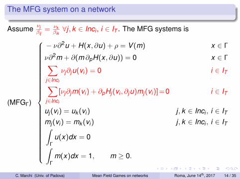
The MFG systems on networks

Theorem (Camilli-M., SJCO ’16)We assume

Hj ∈ C2(ej × R), convex, with δ|p|2 − C ≤ Hj(x ,p) ≤ δ|p|2 + C,νj > 0,V ∈ C1([0,+∞)).

Then, there exists a solution (u,m, ρ) ∈ C2(Γ)× C2(Γ)× R to (MFGΓ).

Moreover, assumeeither V is strictly monotone in mor V is monotone in m and H is strictly convex in p.

The MFG systems on networks

Theorem (Camilli-M., SJCO ’16)We assume

Hj ∈ C2(ej × R), convex, with δ|p|2 − C ≤ Hj(x ,p) ≤ δ|p|2 + C,νj > 0,V ∈ C1([0,+∞)).

Then, there exists a solution (u,m, ρ) ∈ C2(Γ)× C2(Γ)× R to (MFGΓ).

Moreover, assumeeither V is strictly monotone in mor V is monotone in m and H is strictly convex in p.

Sketch of the proof

Step 1: On the HJB equation.

For f ∈ C0,α(Γ), ∃!(u, ρ) ∈ C2(Γ)× R solution to

−ν∂2u + H(x , ∂u) + ρ = f (x), x ∈ Γ∑

j∈Inciνj∂ju(vi) = 0 i ∈ IT

uj(vi) = uk (vi) j , k ∈ Inci , i ∈ IT∫Γ u(x) = 0.

Moreover u ∈ C2,α(Γ) and: ‖u‖C2,α(Γ) ≤ C, |ρ| ≤ maxΓ |H(·,0)− f (·)|.

The proof is based on∃uλ ∈W 1,2(Γ), weak solution to the discounted approximation

−ν∂2uλ + H(x , ∂uλ) + λuλ = f (x) x ∈ Γ

as in [Boccardo-Murat-Puel,’83]; the Comparison Principle applies;uλ ∈ C2,α(Γ) by the 1-d of the problem and Sobolev theorem;as λ→ 0+, λuλ → ρ and (uλ −min uλ)→ u.

Step 2: On the FP equation.

For b ∈ C1(Γ), there exists a unique weak solution m ∈W 1,2(Γ) to

ν∂2m + ∂(b(x) m) = 0 x ∈ Γ∑

j∈Inci[b(vi)mj(vi) + νj∂jm(vi)] = 0 i ∈ IT

mj(vi) = mk (vi) j , k ∈ Inci , i ∈ ITm ≥ 0,

∫Γ m(x)dx = 1.

Moreover, m is a classical solution with ‖m‖H1 ≤ C, 0 < m(x) ≤ C (forsome C > 0 depending only on ‖b‖∞ and ν).

The proof is based onthe existence of a weak solution is based on the theory of bilinearforms;the adjoint problem (both equation and transition condition) fulfillsthe Maximum Principle;m ∈ C2(Γ) by the 1-d of the problem and Sobolev theorem.

Step 3: Fixed point argument.

We set K := {µ ∈ C0,α(Γ) : µ ≥ 0,∫

Γ µdx = 1} and we define anoperator T : K → K according to the scheme

µ→ u → m

as follows:given µ ∈ K, solve (HJB) with f (x) = V (µ(x)) for the unknownsu = uµ and ρ, which are uniquely defined by Step 1;given uµ, solve (FP) with b(x) = ∂pH(x , ∂uµ) for the unknown mwhich is uniquely defined by Step 2;set T (µ) := m.

Since T is continuous with compact image, Schauder’s fixed pointtheorem ensures the existence of a solution.

Step 4: Uniqueness.

Cross-testing the equations in (MFGΓ), by the transition conditions, weget∑j∈J

(m1 −m2)(V (m1)− V (m2))dx︸︷︷︸≥0 by monotonicity

∑j∈J

m1[Hj(x , ∂ju2)− Hj(x , ∂ju1)− ∂pHj(x , ∂ju1)∂j(u2 − u1)

]︸︷︷︸≥0 by convexity

∑j∈J

m2[(Hj(x , ∂ju1)− Hj(x , ∂ju2)− ∂pHj(x , ∂ju2)∂j(u1 − u2)

]︸︷︷︸≥0 by convexity

dx = 0.

Therefore, each one of these three lines must vanish and we concludeas in [Lasry-Lions ’06].

A finite difference scheme for MFG on network

We introduce a grid on Γ. For the parametrization πj : [0, lj ]→ Rn

of ej , let yj,k = khj (k = 0, . . . ,Nhj ) be an uniform partition of [0, lj ]:

Gh = {xj,k = πj(yj,k ), j ∈ J, k = 0, . . . ,Nhj }.

Inc+i := {j ∈ Inci : vi = πj(0)}, Inc−i := {j ∈ Inci : vi = πj(Nh

j hj)}.We introduce the (1-dimensional) finite difference operators

(D+U)j,k =Uj,k+1 − Uj,k

hj, [DhU]j,k =

((D+U)j,k , (D+U)j,k−1

(D2hU)j,k =

Uj,k+1 + Uj,k−1 − 2Uj,k

We introduce the inner product. For U,W : Gh → R, set

(U,W )2 =∑j∈J

Nhj −1∑

hjUj,k Wj,k +∑i∈I

( ∑j∈Inc+

2Uj,0Wj,0+

∑j∈Inc−

2Uj,Nh

jWj,Nh

We introduce the numerical Hamiltonian gj : [0, lj ]× R2 → R, s.t.:

(G1) monotonicity: gj(x ,q1,q2) is nonincreasing with respect to q1and nondecreasing with respect to q2.

(G2) consistency: gj (x ,q,q) = Hj(x ,q), ∀x ∈ [0, lj ], ∀q ∈ R.

(G3) differentiability: gj is of class C1.

(G4) superlinear growth : gj(x ,q1,q2) ≥ α((q−1 )2 + (q+2 )2)γ/2 − C

for some α > 0, C ∈ R and γ > 1.

(G5) convexity : (q1,q2)→ gj (x ,q1,q2) is convex.We introduce a continuous numerical potential Vh such that ∃Cindependent of h such that

maxj,k|(Vh[M])j,k | ≤ C, |(Vh[M])j,k − (Vh[M])j,`| ≤ C|yj,k − yj,`|.

for all M ∈ Kh := {M : M is continuous, Mj,k ≥ 0, (M,1)2 = 1}.

We get the following system in the unknown (U,M,R)

− νj (D2hU)j,k + g(xj,k , [DhU]j,k ) + R = Vh(Mj,k )

νj (D2hM)j,k + Bh(U,M)j,k = 0,∑

j∈Inc+i

[νj (D+U)j,0 +

2(Vj,0 − R)

]−∑

j∈Inc−i

[νj (D+U)j,Nh

j −1 −hj

2(Vj,Nh

j− R)

∑j∈Inc+

[νj (D+M)j,0 + Mj,1

∂g∂q2

(xj,1, [DhU]j,1)]−

∑j∈Inc−

[νj (D+M)j,Nh

j −1 + Mj,Nhj −1

∂g∂q1

(xj,Nhj −1, [DhU]j,Nh

j −1)]

U, M continuous at vi , i ∈ I,

(M,1)2 = 1, (U,1)2 = 0,

Theorem (Cacace-Camilli-M., M2AN’17)For any h = {hj}j∈J , the discrete problem has at least a solution(Uh,Mh, ρh). Moreover

|ρh| ≤ C1, ‖Uh‖∞ + ‖DhUh‖∞ ≤ C2

for some constants C1, C2 independent of h.Moreover, if Vh is strictly monotone, then the solution is unique.If (u,m, ρ) is the solution of the MFG system (MFGΓ), then

lim|h|→0

[‖Uh − u‖∞ + ‖Mh −m‖∞ + |ρh − ρ|

Theorem (Cacace-Camilli-M., M2AN’17)For any h = {hj}j∈J , the discrete problem has at least a solution(Uh,Mh, ρh). Moreover

|ρh| ≤ C1, ‖Uh‖∞ + ‖DhUh‖∞ ≤ C2

for some constants C1, C2 independent of h.Moreover, if Vh is strictly monotone, then the solution is unique.If (u,m, ρ) is the solution of the MFG system (MFGΓ), then

lim|h|→0

[‖Uh − u‖∞ + ‖Mh −m‖∞ + |ρh − ρ|

Solution of the discrete MFG system via Nonlinear-Least-Squares

The solution of the MFG discrete system is usually performed bymeans of some regularizations, e.g. large time approximation orergodic approximation. We propose a different method:•We collect the unknowns in a vector X = (U,M,R) of length 2Nh + 1;• we consider the nonlinear map F : R2Nh+1 → R2Nh+2 defined by

F(X ) =

−νj(D2hU)j,k + g(xj,k , [DhU]j,k ) + R − Vh(Mj,k ), k = 1, . . . ,Nh

j − 1, j ∈ J

νj(D2hM)j,k + Bh(U,M)j,k , k = 1, . . . ,Nh

j − 1, j ∈ J∑j∈Inc+

[νj(D+U)j,0 +

2(Vj,0 − R)

]−∑

j∈Inc−i

[νj(D+U)j,Nh

j −1 −hj

2(Vj,Nh

j− R)

]i ∈ I

∑j∈Inc+

[νj(D+M)j,0 + Mj,1

∂g∂q2

(xj,1, [DhU]j,1)]

−∑

j∈Inc−i

[νj(D+M)j,Nh

j −1 + Mj,Nhj −1

∂g∂q1

j −1)]

(M, 1)2 − 1

(U, 1)2.

• The solution of the discrete MFG is the unique X ? s.t. F(X ?) = 0.C. Marchi (Univ. of Padova) Mean Field Games on networks Roma, June 14th, 2017 24 / 35

F(X ) =

j − 1, j ∈ J

j − 1, j ∈ J∑j∈Inc+

[νj(D+U)j,0 +

2(Vj,0 − R)

]−∑

j∈Inc−i

[νj(D+U)j,Nh

j −1 −hj

2(Vj,Nh

j− R)

]i ∈ I

∑j∈Inc+

[νj(D+M)j,0 + Mj,1

∂g∂q2

(xj,1, [DhU]j,1)]

−∑

j∈Inc−i

[νj(D+M)j,Nh

j −1 + Mj,Nhj −1

∂g∂q1

j −1)]

(M, 1)2 − 1

(U, 1)2.

F(X ) =

j − 1, j ∈ J

j − 1, j ∈ J∑j∈Inc+

[νj(D+U)j,0 +

2(Vj,0 − R)

]−∑

j∈Inc−i

[νj(D+U)j,Nh

j −1 −hj

2(Vj,Nh

j− R)

]i ∈ I

∑j∈Inc+

[νj(D+M)j,0 + Mj,1

∂g∂q2

(xj,1, [DhU]j,1)]

−∑

j∈Inc−i

[νj(D+M)j,Nh

j −1 + Mj,Nhj −1

∂g∂q1

j −1)]

(M, 1)2 − 1

(U, 1)2.

The system F(X ?) = 0 is formally overdetermined (2Nh + 2 equationsin 2Nh + 1 unknowns), hence the solution is meant in the followingnonlinear-least-squares sense:

X ? = arg minX

12‖F(X )‖22 .

The previous optimization problem is solved by means of theGauss-Newton method

JF (X k )δX = −F(X k ), X k+1 = X k + δX .

via the QR factorization of the Jacobian JF (X k ).

Numerical experiments

We consider a network with 2 vertices and 3 edges (boundary verticesare identified!). Each edge has unit length and connects (0,0) to(cos(2πj/3), sin(2πj/3)) with j = 0,1,2.

• Uniform diffusion νj ≡ ν• Hj(x ,p) = 1

2 |p|2 + f (x)

f (x) = sj

(1 + cos(2π

(x + 1

sj ∈ {0,1}• V [m] = m2

-0.5 0 0.5 1

Computational time for Nh ∼ 5000 is of the order of seconds!C. Marchi (Univ. of Padova) Mean Field Games on networks Roma, June 14th, 2017 26 / 35

Cost active on all edges

ν = 0.1, s0 = 1, s1 = 1, s2 = 1, V [m] = m2

-0.5 0 0.5 1

1 -1-0.8

-0.6-0.4

0.20.4

0.60.8

-0.2-0.1

00.10.20.30.40.50.60.70.8

M M (blu) and U (red)

Computed ρ = −1.066667C. Marchi (Univ. of Padova) Mean Field Games on networks Roma, June 14th, 2017 27 / 35

Cost active on two edges

ν = 0.1, s0 = 1, s1 = 1, s2 = 0, V [m] = m2

-0.5 0 0.5 1

-0.6 -0.4 -0.2 0 0.2 0.4 0.6 0.8 1-1-0.8-0.6-0.4-0.200.20.40.60.81-0.4

Small viscosity, cost active on all edges

ν = 10−4, s0 = 1, s1 = 1, s2 = 1, V [m] = m2

-0.5 0 0.5 1

1 -1-0.8

-0.6-0.4

0.20.4

0.60.8

Small viscosity, cost active on two edges

ν = 10−4, s0 = 1, s1 = 1, s2 = 0, V [m] = m2

-0.5 0 0.5 1

-0.6-0.4

0.20.4

0.60.8

1 -1-0.8

-0.6-0.4

0.20.4

0.60.8

ν = 0.1, s0 = 1, s1 = 1, s2 = 1, V [m] = 1− 4πarctan(m)

-0.5 0 0.5 1

1 -1-0.8

-0.6-0.4

0.20.4

0.60.8

M M and U

Computed Λ = −1.219979

ν = 10−3, s0 = 1, s1 = 1, s2 = 1, V [m] = 1− 4πarctan(m)

-0.5 0 0.5 1

1 -1-0.8

-0.6-0.4

0.20.4

0.60.8

M M and U

Computed Λ = −2.832411

More complex networks

-2 0 2 4 6 8 10 12

Comments and Remarks:

rigorous derivation of the system starting from the game with Nplayers.more general transitions conditions (arbitrary weights for theedges, controlled weights...) and/or lack of continuity condition.first order MFG systems on networks.

Thank You!

mean field games on networks - uniroma1.it · mean field games on networks claudio marchi ......

Documents