Mean-Variance Portfolio Analysisand the

Capital Asset Pricing Model

1 Introduction

In this handout we develop a model that can be used to determine how a risk-averse investorcan choose an optimal asset portfolio in this sense:

• the investor will earn the highest possible expected return given the level of volatility theinvestor is willing to accept or, equivalently,

• the investor’s portfolio will have the lowest level of volatility given the level of expectedreturn the investor requires.

The techniques used are called mean-variance optimization and the underlying theory is calledthe Capital Asset Pricing Model (CAPM). Under the assumptions of CAPM, it is possible todetermine the expected “risk-adjusted” return of any asset/security, which incorporates thesecurity’s expected return, volatility and its correlation with the “market portfolio.”

1

2 Market Setup

We consider a market with n risky assets, i = 1, 2, . . . , n and a risk-free asset labeled 0. Aninvestor wishes to invest B dollars in this market. Let

• Bi, i = 0, 1, 2, . . . , n, denote the allocation of the budget to asset i so that∑ni=0Bi = B,

• xi := Bi/B denote the portfolio weight of asset i, namely, the fraction of the investor’sbudget allocated to asset i,

• Ri denote the random one-period return on asset i, i = 1, 2, . . . , n, and let

• rf denote the risk-free return.

The investor’s one-period return on his/her portfolio is given by

One-period return =

∑ni=0BiRiB

=n∑i=0

BiB

Ri =n∑i=0

xiRi. (1)

We shall think of B as fixed and hereafter identify a portfolio of the n+ 1 assets with a vector

x = (x0, x1, x2, . . . , xn) such thatn∑i=0

xi = 1. (2)

The portfolio’s random return will be denoted by

RP = R(x) :=n∑i=1

xiRi. (3)

We shall use the symbols ‘x’ or P to refer to a portfolio.

When xi < 0 the holder of the portfolio is short-selling asset i. In this handout we permitunlimited short-selling. In practice, however, there are limits to the magnitude of short-selling.If short-selling is not permitted, then the solution approach outlined in these notes does notdirectly apply, though the problem can be easily solved with commercial software.

2

Example 1 Consider a portfolio of 200 shares of firm A worth $30/share and 100 shares offirm B worth $40/share. The total value of the portfolio is

200($30) + 100($40) = $10, 000. (4)

The respective portfolio weights are

xA =200($30)

$10, 000= 60%, xB =

100($40)

$10, 000= 40%. (5)

Example 2 Suppose you bought the portfolio of Example 1, and suppose further that firmA’s share price goes up to $36 and firm B’s share price falls to $38.

• What is the new value of the portfolio?

The new value of the portfolio is

200 ∗ ($36) + 100($38) = $11, 000. (6)

• What return did this portfolio earn?

The portfolio’s gain was $1,000 or 10% return on investment.A’s return was 36/30 - 1 = 20% and B’s return was 38/40 - 1 = -5%.

Since the initial portfolio weights are xA = 60% and xB = 40%, we can also compute theportfolio’s return as

RP = xARA + xBRB = 0.60(20%) + 0.40(−5%) = 10%. (7)

• After the price change, what are the new portfolio weights?

The new portfolio weights are

xA =200($36)

$11, 000= 65.45%, xB =

100($38)

$11, 000= 34.55%. (8)

3

3 Portfolio Return

The expected return of a portfolio P is given by

µ(x) := E[RP ] = E[∑i

xiRi] =∑i

E[xiRi] =∑i

xiE[Ri]. (9)

Example 3 You invest $1000 in stock A, $3000 in stock B. You expect a return of 10% forstock A and 18% in stock B.

• What is your portfolio’s expected return?

Your portfolio weights are xA = 1, 000/4, 000 = 25% and xB = 3, 000/4, 000 = 75%.Therefore,

E[RP ] = 0.25(10%) + 0.75(18%) = 16%. (10)

4

4 Portfolio Variance: Basic definitions and properties

Let

R̄i := E[Ri] (11)

V ar[Ri] := E(Ri − R̄i)2 = E[R2i ]− (R̄i)

2 (12)

σi :=√V ar[Ri] (13)

denote, respectively, the mean, variance and standard deviation of Ri.

The covariance between two random variables X and Y is defined as

Cov(X,Y ) = σXY := E[(X − E[X])(Y − E[Y ])] = E[XY ]− E[X]E[Y ], (14)

and the correlation between two random variables X and Y is defined as

Corr(X,Y ) = ρXY :=Cov(X,Y )

σXσY(15)

A correlation value must always be a number between -1 and 1. The covariance can be deter-mined from correlation via

σXY = Cov(X,Y ) = Corr(X,Y )σXσY = ρXY σXσY . (16)

It follows directly from (14) that

• variance may be expressed in terms of covariance:

V ar(X) = Cov(X,X), (17)

• covariance is symmetric:

Cov(X,Y ) = Cov(Y,X), (18)

• covariance is bilinear :

Cov(n∑i=1

Xi,m∑j=1

Yj) =n∑i=1

Cov(Xi,m∑j=1

Yj) =n∑i=1

m∑j=1

Cov(Xi, Yj), (19)

Cov(αX, Y ) = Cov(X,αY ) = αCov(X,Y ), α a real number. (20)

5

5 Portfolio Variance Formula

Let

σij := Cov(Ri, Rj) = σiσjCorr(Ri, Rj) = σiσjρij (21)

denote the covariance between the returns of assets i and j, and let Σ denote the n by n matrixwhose (i, j)th entry is given by σij .

The matrix Σ is called the covariance matrix. Due to (18), σij = σji, which implies thatthe covariance matrix is symmetric, namely, Σ = ΣT (here, the symbol ‘T’ denotes transpose).

Using (17) and repeated application of (19) and (20), it can be shown that the portfolio’s(return) variance is

V ar[R(x)] =n∑i=1

n∑j=1

σijxixj . (22)

Special Case: n = 2. Here, the portfolio’s variance is

V ar[R(x)] =2∑i=1

2∑j=1

σijxixj = σ21x

21 + σ12x1x2 + σ21x2x1 + σ2

2x22 (23)

= σ21x

21 + σ2

2x22 + 2σ12x1x2 (24)

= σ21x

21 + σ2

2x22 + 2σ1σ2ρ12x1x2 (25)

The last line usees the fact that σ12 and σ21 are equal.

General Case. In matrix notation, the portfolio’s variance may be represented as

V ar[R(x)] = xTΣx (26)

=(x1 x2

)( σ21 σ12

σ21 σ22

)(x1

x2

)(27)

=(x1 x2

)( σ21x1 + σ12x2

σ21x1 + σ22x2

)(28)

= (x1σ21x1 + x1σ12x2) + (x2σ21x1 + s2σ

22x2) (29)

= σ21x

21 + σ2

2x22 + 2σ12x1x2. (30)

6

Example 4 Stock returns will be more highly correlated when they are similarly affected by thesame economic events. This is why stocks in the same industry tend to have highly correlatedreturns than stocks in somewhat different industries. Table 1 (Table 11.3, p. 336 in CorporateFinance by Berk and DeMarzo) provides some examples.

Table 1: Historical Annual Volatilities and Correlations for Selected Stocks (basedon monthly returns, 1996-2008).

Alaskan Southwest Ford General GeneralMicrosoft Dell Air Airlines Motor Motors Mills

Volatility (StDev) 37% 50% 38% 31% 42% 41% 18%Correlation with:

Microsoft 1.00 0.62 0.25 0.23 0.26 0.23 0.10Dell 0.62 1.00 0.19 0.21 0.31 0.28 0.07

Alaska Air 0.25 0.19 1.00 0.30 0.16 0.13 0.11Southwest Airlines 0.23 0.21 0.30 1.00 0.25 0.22 0.20

Ford Motor 0.26 0.31 0.16 0.25 1.00 0.62 0.07General Motors 0.23 0.28 0.13 0.22 0.62 1.00 0.02

General Mills 0.10 0.07 0.11 0.20 0.07 0.02 1.00

• What is the covariance between the returns for Microsoft and Dell?

Cov(RM , RD) = σmσDρMD = (0.37)(0.50)(0.62) = 0.1147. (31)

• What is the standard deviation of a portfolio with equal amounts invested in these twostocks?

V ar(RP ) = V ar(0.5Rm + 0.5RD) (32)

= σ2Mx

2M + σ2

Dx2D + 2σMDxMxD (33)

= (0.37)2(0.5)2 + (0.5)2(0.5)2 + 2(0.1147) = 0.1541 (34)

σP =√

0.1541 = 39.26%. (35)

7

Example 5 Consider a portfolio of Intel and Coca-Cola stocks.

• Intel’s expected return is 26% and its volatility is 50%.

• Coca-Cola’s expected return is 6% and its volatility is 25%.

• The stock returns are independent, and so the correlation coefficient ρ = 0.

Suppose you have $20,000 in cash to invest. You decide to short sell $10,000 worth of Coco-Colastock and invest the proceeds from your short sale plus your $20,000 in Intel.

• What are the portfolio weights?

Your short sale is a negative investment of $10,000 in Coca-Cola stock. You have invested$30,000 in Intel. Your total investment is still $20,000. Your portfolio weights are 1.5 or150% in Intel and -0.5 or -50% in Coca-Cola.

• What is the portfolio’s expected return?

The expected portfolio return is

1.5(0.26) +−0.5(0.06) = 36%. (36)

• What is the portfolio’s volatility?

The variance of the portfolio return (25) is

0.502(1.5)2 + 0.252(−0.5)2 = 0.578125. (37)

The standard deviation or volatility of the portfolio’s return is

√0.578125 = 0.76 = 76%. (38)

By short-selling you have dramatically increased the expected return but you have also signifi-cantly increased the volatility.

8

6 Minimum Variance Portfolio of Two Assets

The minimum variance portfolio achieves the lowest variance, regardless of expected return.For two assets, it is easy to solve for the minimum variance portfolio. (We shall see that it isalso easy to solve for the minimum variance portfolio for the general case.)

From the two-asset portfolio variance formula (24) with x2 = 1− x1, the variance is

V ar(x1R1 + (1− x1)R2) = σ21x

21 + σ2

2(1− x1)2 + 2x1(1− x1)σ12. (39)

Since there are no constraints on the values for x1, we can take the derivative with respect tox1 and set equal to zero:

0 :=d

dx1V ar(R(x1)) = 2σ2

1x1 − 2(1− x1)σ22 + 2σ12(1− 2x1) (40)

= 2(σ21 + σ2

2 − 2σ12)x1 − 2(σ22 − σ12). (41)

Thus,

x∗1 =σ2

2 − σ12

σ21 + σ2

2 − 2σ12, x∗2 =

σ21 − σ12

σ21 + σ2

2 − 2σ12. (42)

9

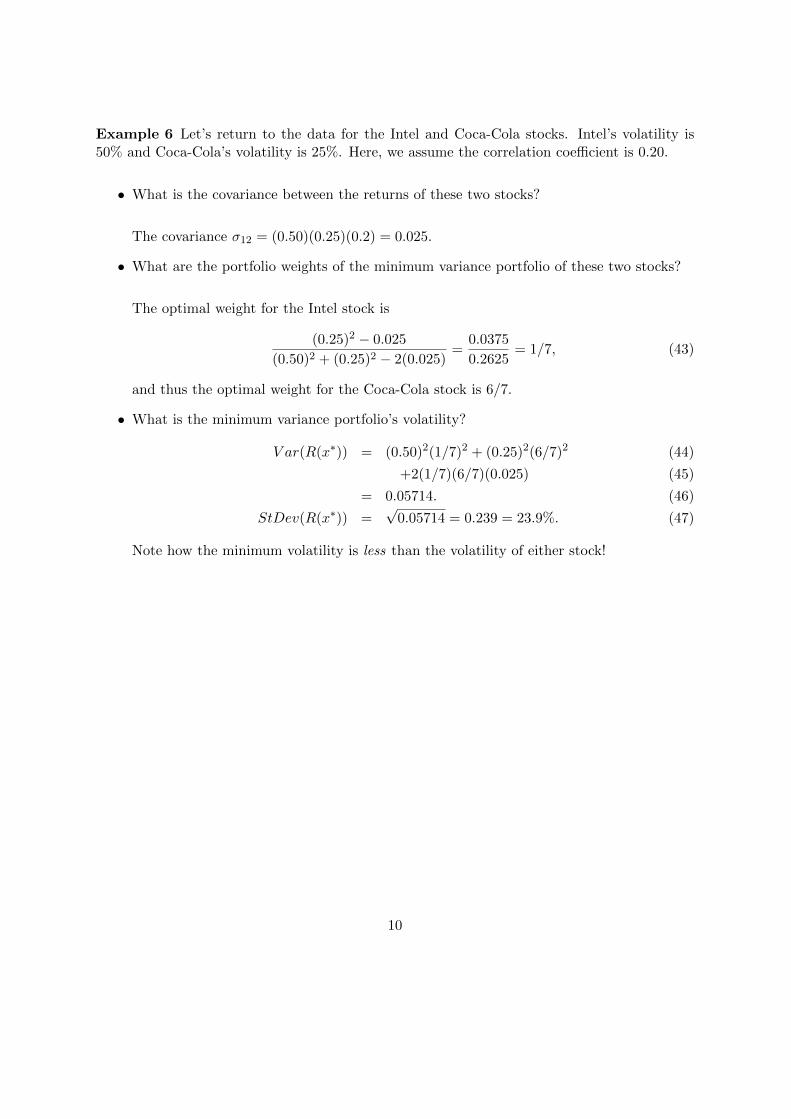
Example 6 Let’s return to the data for the Intel and Coca-Cola stocks. Intel’s volatility is50% and Coca-Cola’s volatility is 25%. Here, we assume the correlation coefficient is 0.20.

• What is the covariance between the returns of these two stocks?

The covariance σ12 = (0.50)(0.25)(0.2) = 0.025.

• What are the portfolio weights of the minimum variance portfolio of these two stocks?

The optimal weight for the Intel stock is

(0.25)2 − 0.025

(0.50)2 + (0.25)2 − 2(0.025)=

0.0375

0.2625= 1/7, (43)

and thus the optimal weight for the Coca-Cola stock is 6/7.

• What is the minimum variance portfolio’s volatility?

V ar(R(x∗)) = (0.50)2(1/7)2 + (0.25)2(6/7)2 (44)

+2(1/7)(6/7)(0.025) (45)

= 0.05714. (46)

StDev(R(x∗)) =√

0.05714 = 0.239 = 23.9%. (47)

Note how the minimum volatility is less than the volatility of either stock!

10

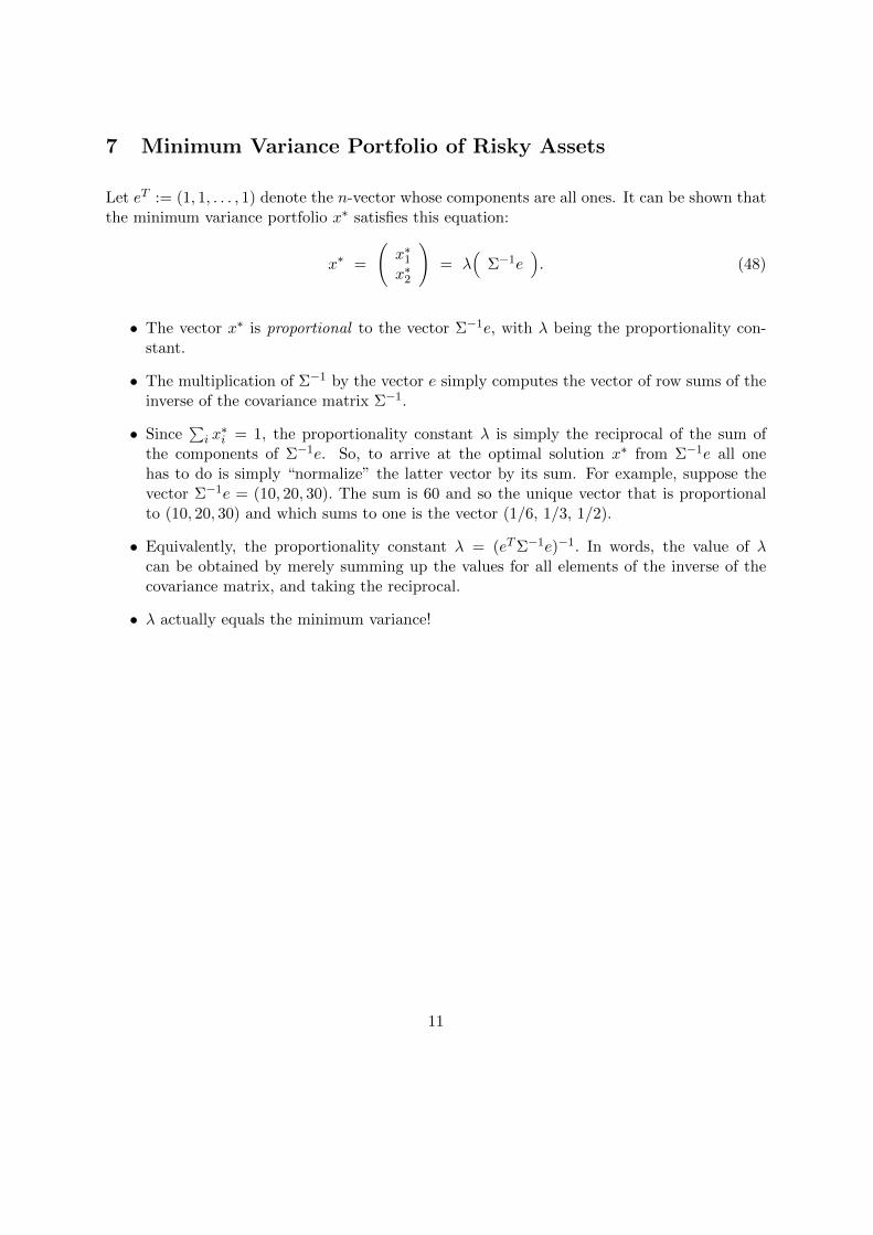
7 Minimum Variance Portfolio of Risky Assets

Let eT := (1, 1, . . . , 1) denote the n-vector whose components are all ones. It can be shown thatthe minimum variance portfolio x∗ satisfies this equation:

x∗ =

(x∗1x∗2

)= λ

(Σ−1e

). (48)

• The vector x∗ is proportional to the vector Σ−1e, with λ being the proportionality con-stant.

• The multiplication of Σ−1 by the vector e simply computes the vector of row sums of theinverse of the covariance matrix Σ−1.

• Since∑i x∗i = 1, the proportionality constant λ is simply the reciprocal of the sum of

the components of Σ−1e. So, to arrive at the optimal solution x∗ from Σ−1e all onehas to do is simply “normalize” the latter vector by its sum. For example, suppose thevector Σ−1e = (10, 20, 30). The sum is 60 and so the unique vector that is proportionalto (10, 20, 30) and which sums to one is the vector (1/6, 1/3, 1/2).

• Equivalently, the proportionality constant λ = (eTΣ−1e)−1. In words, the value of λcan be obtained by merely summing up the values for all elements of the inverse of thecovariance matrix, and taking the reciprocal.

• λ actually equals the minimum variance!

11

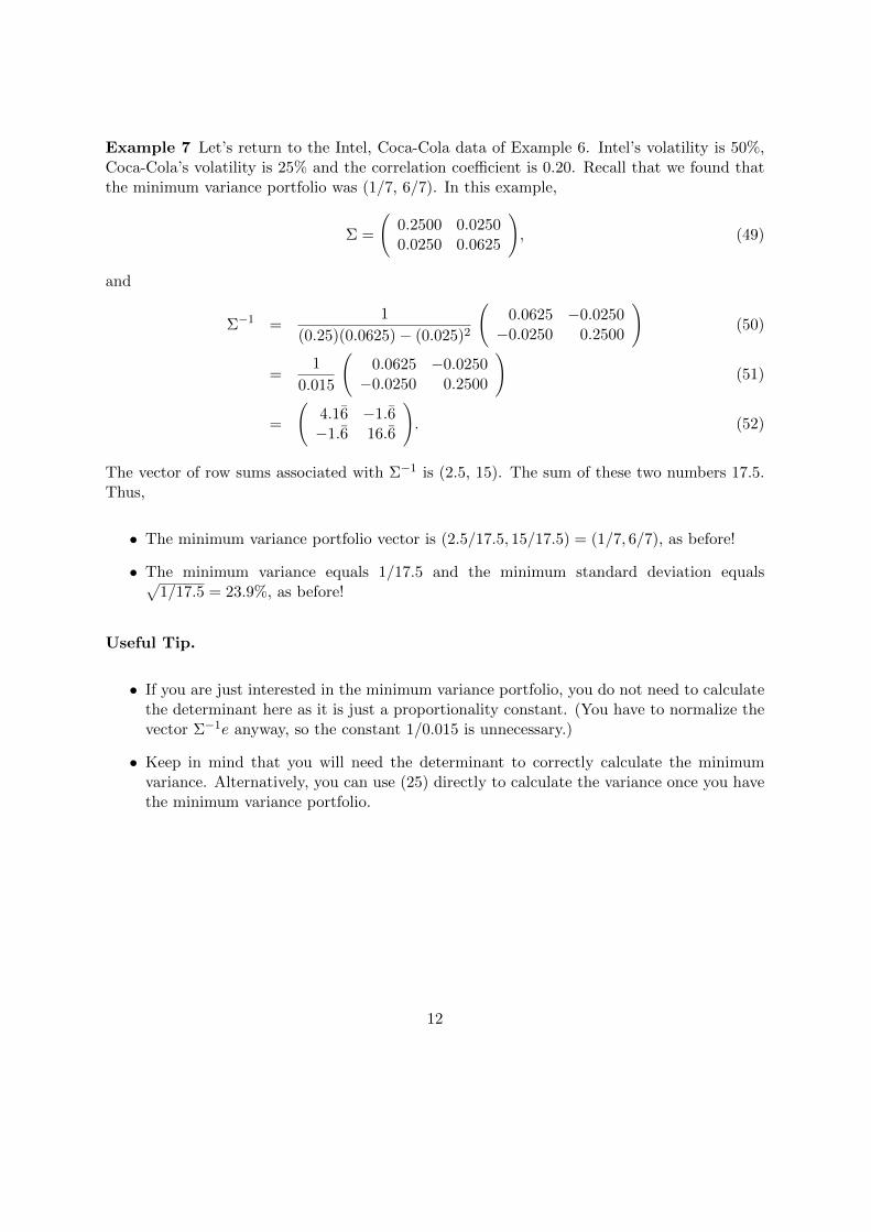
Example 7 Let’s return to the Intel, Coca-Cola data of Example 6. Intel’s volatility is 50%,Coca-Cola’s volatility is 25% and the correlation coefficient is 0.20. Recall that we found thatthe minimum variance portfolio was (1/7, 6/7). In this example,

Σ =

(0.2500 0.02500.0250 0.0625

), (49)

and

Σ−1 =1

(0.25)(0.0625)− (0.025)2

(0.0625 −0.0250−0.0250 0.2500

)(50)

=1

0.015

(0.0625 −0.0250−0.0250 0.2500

)(51)

=

(4.16̄ −1.6̄−1.6̄ 16.6̄

). (52)

The vector of row sums associated with Σ−1 is (2.5, 15). The sum of these two numbers 17.5.Thus,

• The minimum variance portfolio vector is (2.5/17.5, 15/17.5) = (1/7, 6/7), as before!

• The minimum variance equals 1/17.5 and the minimum standard deviation equals√1/17.5 = 23.9%, as before!

Useful Tip.

• If you are just interested in the minimum variance portfolio, you do not need to calculatethe determinant here as it is just a proportionality constant. (You have to normalize thevector Σ−1e anyway, so the constant 1/0.015 is unnecessary.)

• Keep in mind that you will need the determinant to correctly calculate the minimumvariance. Alternatively, you can use (25) directly to calculate the variance once you havethe minimum variance portfolio.

12

Example 8 Consider three risky assets whose covariance matrix Σ is

Σ =

216 70 −32470 25 −150

−324 −150 1596

. (53)

(Here, the returns were measured in percents.) The inverse of the covariance matrix is

Σ−1 =

0.1480 −0.5367 −0.0204−0.5367 2.0388 0.0827−0.0204 0.0827 0.0043

. (54)

Thus,

Σ−1e =

−0.40811.59710.0661

(55)

eTΣ−1e = −0.4081 + 1.5971 + 0.0661 = 1.2379. (56)

• Dividing the vector (−0.4081, 1.5971, 0.0661) by 1.2379 yields (−0.3297, 1.2756, 0.0534),and this is the minimum variance portfolio.

• The sum of all entries of Σ−1 is 1.2379, and this value equals the reciprocal of the minimumvariance. Consequently, the minimum variance portfolio’s volatility is√

1/1.2379 = 0.8078 = 80.78%.

13

8 Volatility of a Large Portfolio: The benefits of diversification

Let AvgV ar denote the average variance of the individual stocks, and let AvgCov denote theaverage covariance between the stocks. Imagine a world where the variance of each stock wasconstant and equal to AvgV ar and the covariance between stocks was constant and equal toAvgCov.

Now consider an equally-weighted portfolio of theses stocks in which xi = 1/n for eachi = 1, 2, . . . , n. What is the variance of this equally-weighted portfolio? The covariance matrixΣ has n2 entries, n along the diagonal and n2 − n = n(n− 1) off-diagonal entries. The entriesalong the diagonal correspond to each stock’s variance which equals AvgV ar, whereas the off-diagonal entries correspond to the covariances which each equal AvgCov. Therefore, in thisspecial setting

V ar(RP ) =AvgV ar

n+

(1− 1

n

)∗AvgCov. (57)

We can see that V ar(RP ) → AvgCov as n → ∞. The limiting portfolio standard deviationStDev(RP ) =

√AvgCov.

The historical volatility (standard deviation) of the return of a large stock is about 40% andthe typical correlation between the returns of large stocks is about 28%. On average, then,

AvgV ar = (0.40)2 = 0.16, (58)

AvgCov = (0.40)(0.40)(0.28) = 0.0448, (59)

StDev(Rp) =√

0.16/n+ 0.0448(1− 1/n) −→ 21.17%. (60)

Note that when n = 20 the StDev(Rp) = 22.49%, which is very close to the limiting volatility.

What about a portfolio with arbitrary weights? It can be shown that

V ar(RP ) = σ2P =

∑i

xiσiσPCorr(Ri, RP ). (61)

Dividing both sides of this equation by σP yields this very important decomposition of thevolatility of a portfolio:

StDev(RP ) =∑i

Security i’s contribution to volatility of P︷ ︸︸ ︷xi︸︷︷︸

Amount of i held

∗ σi︸︷︷︸Total risk of i

∗ Corr(Ri, RP )︸ ︷︷ ︸Fraction of i’s risk common to P

(62)

Assume that not all assets have a perfect positive correlation of +1 and that the weights areall positive. We can conclude that the volatility of the portfolio will be lower than the weightedaverage volatility given by

∑i xiσi. Note how the expected return of a portfolio

∑i xiE[Ri] is

the weighted average of the individual returns. So, you can eliminate some of the volatility bydiversifying.

14

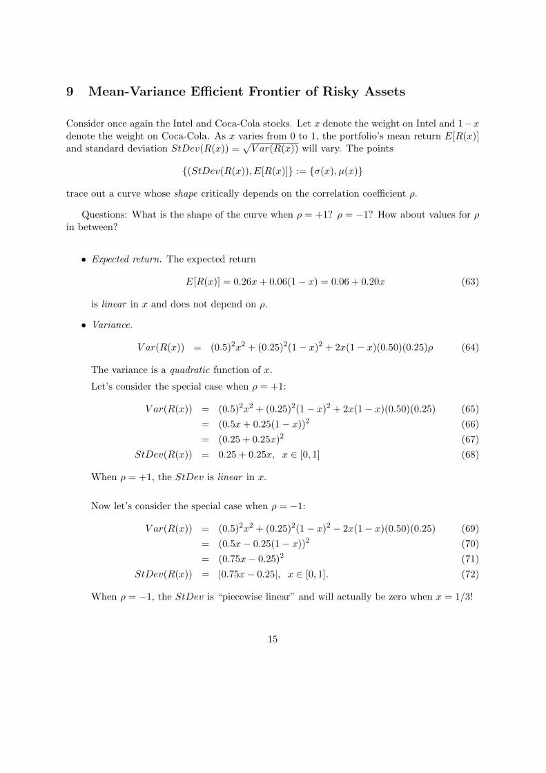
9 Mean-Variance Efficient Frontier of Risky Assets

Consider once again the Intel and Coca-Cola stocks. Let x denote the weight on Intel and 1−xdenote the weight on Coca-Cola. As x varies from 0 to 1, the portfolio’s mean return E[R(x)]and standard deviation StDev(R(x)) =

√V ar(R(x)) will vary. The points

{(StDev(R(x)), E[R(x)]} := {σ(x), µ(x)}

trace out a curve whose shape critically depends on the correlation coefficient ρ.

Questions: What is the shape of the curve when ρ = +1? ρ = −1? How about values for ρin between?

• Expected return. The expected return

E[R(x)] = 0.26x+ 0.06(1− x) = 0.06 + 0.20x (63)

is linear in x and does not depend on ρ.

• Variance.

V ar(R(x)) = (0.5)2x2 + (0.25)2(1− x)2 + 2x(1− x)(0.50)(0.25)ρ (64)

The variance is a quadratic function of x.

Let’s consider the special case when ρ = +1:

V ar(R(x)) = (0.5)2x2 + (0.25)2(1− x)2 + 2x(1− x)(0.50)(0.25) (65)

= (0.5x+ 0.25(1− x))2 (66)

= (0.25 + 0.25x)2 (67)

StDev(R(x)) = 0.25 + 0.25x, x ∈ [0, 1] (68)

When ρ = +1, the StDev is linear in x.

Now let’s consider the special case when ρ = −1:

V ar(R(x)) = (0.5)2x2 + (0.25)2(1− x)2 − 2x(1− x)(0.50)(0.25) (69)

= (0.5x− 0.25(1− x))2 (70)

= (0.75x− 0.25)2 (71)

StDev(R(x)) = |0.75x− 0.25|, x ∈ [0, 1]. (72)

When ρ = −1, the StDev is “piecewise linear” and will actually be zero when x = 1/3!

15

Let’s consider the general case where x = (x1, x2, . . . , xn) denotes a portfolio of risky assets.For each choice of x we can compute the values for its (volatility, mean) = (σ(x), µ(x)). Imaginethat we plot these points in the (σ, µ) plane for all possible portfolio’s x. Which portfolio’s willa risk-averse investor choose?

Fix a value for the expected return, say µ = 10%, and consider all portfolio’s x such thatµ(x) = 10%. Among all such portfolio’s it makes sense to choose one that minimizes thevolatility. Let’s call this minimum volatility σ(µ). As we choose different values for µ we obtaindifferent values for σ(µ). In fact, the collection of all such points {(σ(µ), µ)} in the (σ, µ) planetrace out a “boundary curve.”

We can also fix a value for the volatility, σ = 20%, and consider all portfolio’s x such thatσ(x) = 20%. Among all such portfolio’s it makes sense to choose one that maximizes theexpected return. Let’s call this maximum expected return µ(σ). As we choose different valuesfor σ we obtain different values for µ(σ). In fact, the collection of all such points {(σ, µ(σ))} inthe (σ, µ) plane trace out a “boundary curve,” too. This curve will be identical to the previouscurve.

This boundary curve is called the mean-variance efficient frontier of risky assets.

16

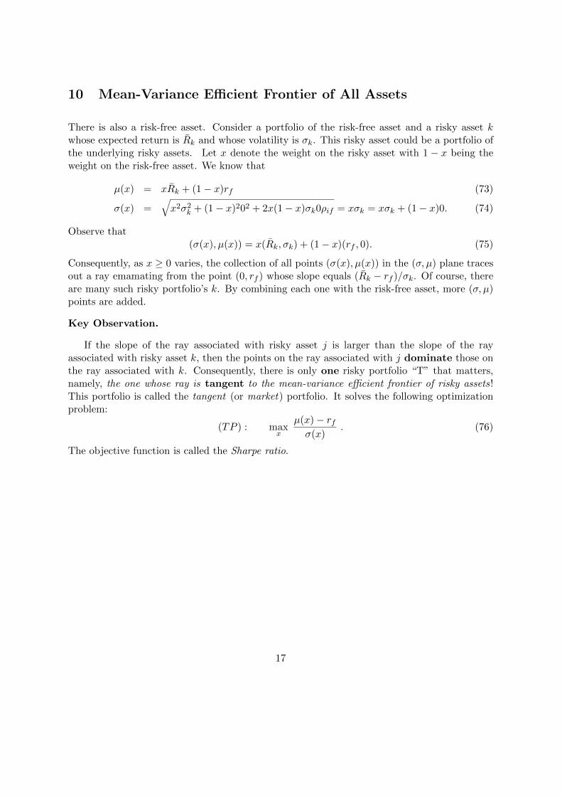
10 Mean-Variance Efficient Frontier of All Assets

There is also a risk-free asset. Consider a portfolio of the risk-free asset and a risky asset kwhose expected return is R̄k and whose volatility is σk. This risky asset could be a portfolio ofthe underlying risky assets. Let x denote the weight on the risky asset with 1 − x being theweight on the risk-free asset. We know that

µ(x) = xR̄k + (1− x)rf (73)

σ(x) =√x2σ2

k + (1− x)202 + 2x(1− x)σk0ρif = xσk = xσk + (1− x)0. (74)

Observe that(σ(x), µ(x)) = x(R̄k, σk) + (1− x)(rf , 0). (75)

Consequently, as x ≥ 0 varies, the collection of all points (σ(x), µ(x)) in the (σ, µ) plane tracesout a ray emamating from the point (0, rf ) whose slope equals (R̄k − rf )/σk. Of course, thereare many such risky portfolio’s k. By combining each one with the risk-free asset, more (σ, µ)points are added.

Key Observation.

If the slope of the ray associated with risky asset j is larger than the slope of the rayassociated with risky asset k, then the points on the ray associated with j dominate those onthe ray associated with k. Consequently, there is only one risky portfolio “T” that matters,namely, the one whose ray is tangent to the mean-variance efficient frontier of risky assets!This portfolio is called the tangent (or market) portfolio. It solves the following optimizationproblem:

(TP ) : maxx

µ(x)− rfσ(x)

. (76)

The objective function is called the Sharpe ratio.

17

11 Application of the Sharpe Ratio

The Sharpe ratio can be used to decide whether adding an asset to a portfolio will be beneficial.Here is the setup. You are given a portfolio P and an asset i not in portfolio P . Will addingasset i improve your portfolio? Adding asset i (either with a positive or negative weight) to Pwill be beneficial if by doing so it will increase the (new) Sharpe ratio.

Example 9 Suppose portfolio P ’s expected return is 12%, its volatility is 20% and the risk-freerate is 3%. Suppose further that a particular mix of asset i and P yields a portfolio P ′ with anexpected return of 18% and a volatility of 30%.

• What is the Sharpe ratio of P?

The Sharpe ratio of P is (0.12-0.03)/0.20 = 0.45.

• What is the Sharpe ratio of P ′?

The Sharpe ratio for P ′ is (0.18-0.03)/0.30 = 0.50.

• Show that asset i is in fact beneficial.

Form a portfolio of P ′ and the risk-free asset with respective weights 2/3 and 1/3. Thisnew portfolio will have a volatility of 2/3(0.30) = 0.20 = 20%, the same as portfolioP . This new portfolio’s expected return is 2/3(18%) + 1/3(3%) = 13%. Thus, this newportfolio has the same volatility but with a higher expected return than P .

Alternatively, form a portfolio of P ′ and the risk-free asset with respective weights 60%and 40%. This new portfolio will have an expected return of 0.60(18%)+0.40(3%) = 12%,the same as portfolio P . This new portfolio’s volatility is 0.60(0.30) = 0.18 = 18%. Thus,this new portfolio has the same expected return but with a lower volatility than P .

18

12 Computing the Tangent Portfolio

All mean-variance efficient portfolios must be a combination of the risk-free security and thetangent portfolio. That is, each investor should allocate a portion of their budget to the risk-free security and the remaining portion to the tangent portfolio. The sub-allocations to theindividual risky securities are determined by the weights x∗ that define the tangent portfolio(to be determined). A very risk-averse investor allocates very little to the tangent portfolio,whereas an investor with a large appetite for risk may hold a negative portion in the risk-freesecurity (i.e. borrow at the risk-free rate) to invest more than the budget into the tangentportfolio.

DefineR̂ := R̄− rfe. (77)

It is the vector of excess returns obtained by simply subtracting the risk-free rate from eachof the asset’s expected returns. It can be shown that the tangent portfolio must be proportionalto Σ−1R̂, and thus it may be found in the analogous way we found the minimum varianceportfolio.

Example 10 Consider again our three asset data of the previous example. Suppose the ex-pected returns are (R̄1, R̄2, R̄3) = (18%, 10%, 8%), and the risk-free rate is 3%.

• What is the vector of excess expected returns?

The vector of excess expected returns is (18%−3%, 10%−3%, 8%−3%) = (15%, 7%, 5%).

• What is the tangent portfolio?

The tangent portfolio is proportional to

Σ−1

1575

=

−1.63896.63460.2944

. (78)

Now divide the right-hand side of (78) by 5.2901 = −1.6389+6.6346+0.2944 to obtain thetangent portfolio as (−0.3098, 1.2542, 0.0557). You may verify that the tangent portfolio’sexpected return is 7.4112% and its volatility equals

√0.8338 = 91.31%.

The fact that the tangent portfolio is proportional to Σ−1R̂ implies a relationship betweena security’s expected return and a measure of its risk. This relationship is called the SecurityMarket Line (SML) and is the most widely used approach to determine an appropriate expectedreturn for a security (or asset). The SML can also be used to decide whether an asset shouldbe added to an existing portfolio and, if so, how to determine its weight in the new portfolio.

19

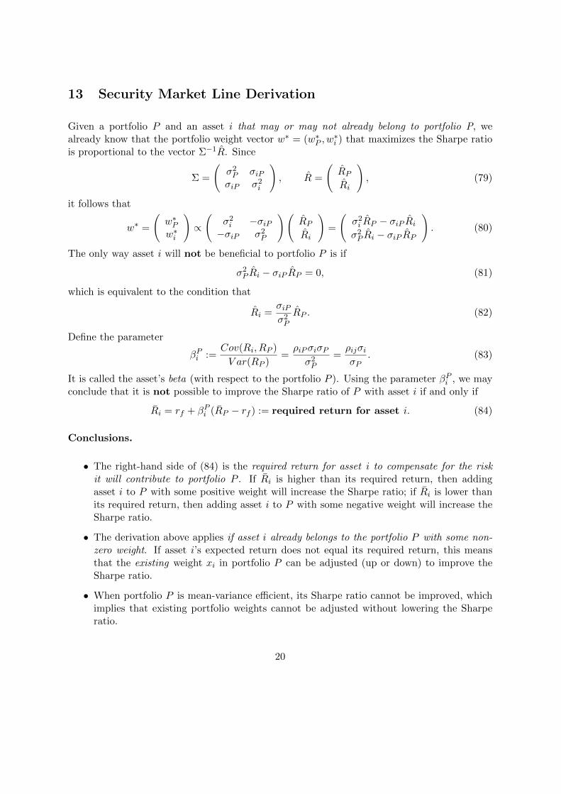
13 Security Market Line Derivation

Given a portfolio P and an asset i that may or may not already belong to portfolio P, wealready know that the portfolio weight vector w∗ = (w∗P , w

∗i ) that maximizes the Sharpe ratio

is proportional to the vector Σ−1R̂. Since

Σ =

(σ2P σiP

σiP σ2i

), R̂ =

(R̂PR̂i

), (79)

it follows that

w∗ =

(w∗Pw∗i

)∝(

σ2i −σiP

−σiP σ2P

)(R̂PR̂i

)=

(σ2i R̂P − σiP R̂i

σ2P R̂i − σiP R̂P

). (80)

The only way asset i will not be beneficial to portfolio P is if

σ2P R̂i − σiP R̂P = 0, (81)

which is equivalent to the condition that

R̂i =σiPσ2P

R̂P . (82)

Define the parameter

βPi :=Cov(Ri, RP )

V ar(RP )=ρiPσiσPσ2P

=ρijσiσP

. (83)

It is called the asset’s beta (with respect to the portfolio P ). Using the parameter βPi , we mayconclude that it is not possible to improve the Sharpe ratio of P with asset i if and only if

R̄i = rf + βPi (R̄P − rf ) := required return for asset i. (84)

Conclusions.

• The right-hand side of (84) is the required return for asset i to compensate for the riskit will contribute to portfolio P . If R̄i is higher than its required return, then addingasset i to P with some positive weight will increase the Sharpe ratio; if R̄i is lower thanits required return, then adding asset i to P with some negative weight will increase theSharpe ratio.

• The derivation above applies if asset i already belongs to the portfolio P with some non-zero weight. If asset i’s expected return does not equal its required return, this meansthat the existing weight xi in portfolio P can be adjusted (up or down) to improve theSharpe ratio.

• When portfolio P is mean-variance efficient, its Sharpe ratio cannot be improved, whichimplies that existing portfolio weights cannot be adjusted without lowering the Sharperatio.

20

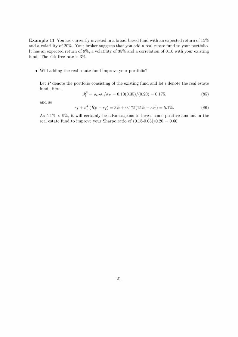
Example 11 You are currently invested in a broad-based fund with an expected return of 15%and a volatility of 20%. Your broker suggests that you add a real estate fund to your portfolio.It has an expected return of 9%, a volatility of 35% and a correlation of 0.10 with your existingfund. The risk-free rate is 3%.

• Will adding the real estate fund improve your portfolio?

Let P denote the portfolio consisting of the existing fund and let i denote the real estatefund. Here,

βPi = ρiPσi/σP = 0.10(0.35)/(0.20) = 0.175, (85)

and sorf + βPi (R̄P − rf ) = 3% + 0.175(15%− 3%) = 5.1%. (86)

As 5.1% < 9%, it will certainly be advantageous to invest some positive amount in thereal estate fund to improve your Sharpe ratio of (0.15-0.03)/0.20 = 0.60.

21

Example 12 Consider the data for the previous example. What is the best combination ofthe broad-based and real estate funds to maximize the Sharpe ratio?

The covariance is σiP = (.35)(0.20)(0.1) = 0.007,

Σ =

(σ2P σiP

σiP σ2i

)=

(0.04 0.0070.007 0.1225

), R̂ =

(R̂PR̂i

)=

(126

). (87)

Consequently,

w∗ =

(w∗Pw∗i

)∝(

0.1225 −0.007−0.007 0.04

)(126

)=

(1.4280.156

), (88)

and so the optimal portfolio weights are

w∗ = (w∗P , w∗i ) =

(1.428

1.428 + 0.15,

0.156

1.428 + 0.156

)= (90.15%, 9.85%). (89)

Suppose you had $10,000 invested in the broad-based portfolio. You could rebalance yourportfolio in two ways:

• Keep the $10,000 in the broad-based portfolio. The optimal portfolio weights imply thatfor every dollar invested in the broad-based fund, you need to invest $0.0985/0.9015 =$0.1093 in the real estate fund. So you need to invest $1,093 in the real estate fund. Youwould borrow this money from at the risk-free rate.

• If you did not wish to borrow funds, you would then sell $985 of the broad-based portfolioand invest the proceeds into the real estate fund. You would then have $9,015 in thebroad-based portfolio, $985 in the real-estate fund, thereby achieving the desired portfolioweights.

22

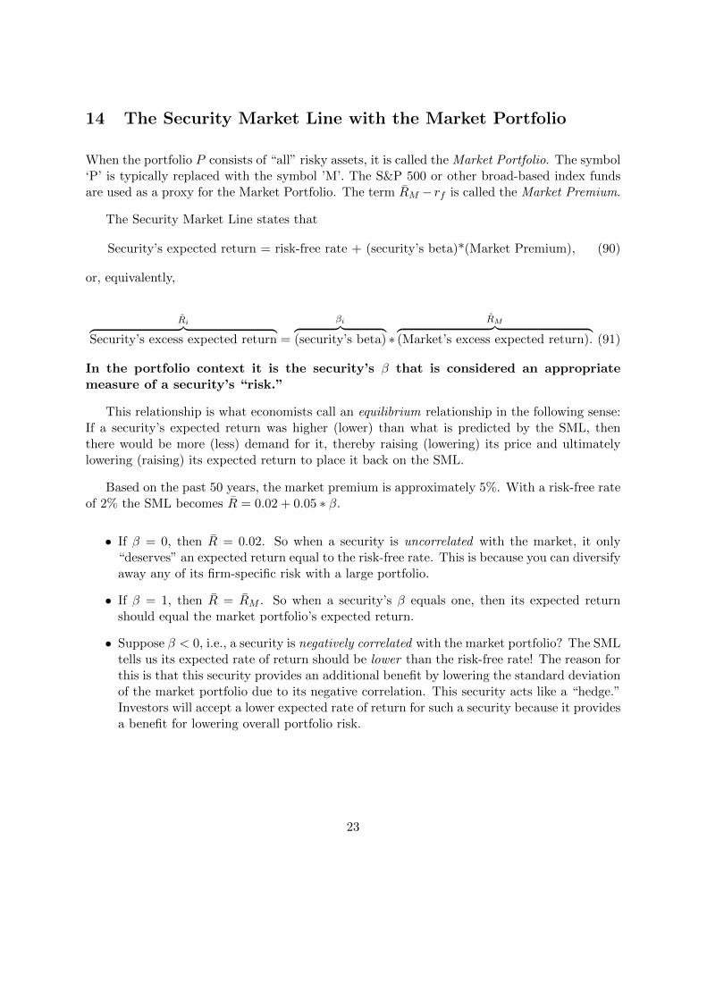
14 The Security Market Line with the Market Portfolio

When the portfolio P consists of “all” risky assets, it is called the Market Portfolio. The symbol‘P’ is typically replaced with the symbol ’M’. The S&P 500 or other broad-based index fundsare used as a proxy for the Market Portfolio. The term R̄M − rf is called the Market Premium.

The Security Market Line states that

Security’s expected return = risk-free rate + (security’s beta)*(Market Premium), (90)

or, equivalently,

R̂i︷ ︸︸ ︷Security’s excess expected return =

βi︷ ︸︸ ︷(security’s beta) ∗

R̂M︷ ︸︸ ︷(Market’s excess expected return). (91)

In the portfolio context it is the security’s β that is considered an appropriatemeasure of a security’s “risk.”

This relationship is what economists call an equilibrium relationship in the following sense:If a security’s expected return was higher (lower) than what is predicted by the SML, thenthere would be more (less) demand for it, thereby raising (lowering) its price and ultimatelylowering (raising) its expected return to place it back on the SML.

Based on the past 50 years, the market premium is approximately 5%. With a risk-free rateof 2% the SML becomes R̄ = 0.02 + 0.05 ∗ β.

• If β = 0, then R̄ = 0.02. So when a security is uncorrelated with the market, it only“deserves” an expected return equal to the risk-free rate. This is because you can diversifyaway any of its firm-specific risk with a large portfolio.

• If β = 1, then R̄ = R̄M . So when a security’s β equals one, then its expected returnshould equal the market portfolio’s expected return.

• Suppose β < 0, i.e., a security is negatively correlated with the market portfolio? The SMLtells us its expected rate of return should be lower than the risk-free rate! The reason forthis is that this security provides an additional benefit by lowering the standard deviationof the market portfolio due to its negative correlation. This security acts like a “hedge.”Investors will accept a lower expected rate of return for such a security because it providesa benefit for lowering overall portfolio risk.

23

What is the beta of a portfolio P? It can be shown that

βP =∑i

xiβi. (92)

That is, the beta of a portfolio is the weighted average of the beta of the assets in the portfolio.

Example 13 Stock A has a beta of 0.50 and Stock B has a beta of 1.25. Suppose rf = 4% andR̄M = 10%. What is the expected return of an equally weighted portfolio of these two stocks?Applying the SML, we have:

R̄A = rf + βA(R̄M − rf ) = 4% + 0.50(10%− 4%) = 7%, (93)

R̄B = rf + βB(R̄M − rf ) = 4% + 1.25(10%− 4%) = 11.5% (94)

Expected return of an equally weighted portfolio is 0.50(7%) + 0.50(11.5%) = 9.25%.

Example 14 Consider the data of the previous example. The portfolio’s beta is0.50(0.50) + 0.50(1.25) = 0.875. Applying the SML again, we have that

R̄P = rf + βP (R̄M − rf ) = 4% + (0.875)(10%− 4%) = 9.25%.

24

15 Estimation of β Via Regression

One can estimate β via linear regression. Its value corresponds to the slope of the best-fittingline in the plot of the security’s excess return versus the market’s excess return. Linear regressionmodels the excess return of a security as the sum of three components:

R̂i = αi + βiR̂M + εi. (95)

• αi is the constant or intercept term of the regression, also called the stock’s alpha.

• βiR̂M represents the sensitivity of the stock to market risk.

• εi is the error (or residual) term. The average error is assumed to be zero.

Taking the expectations of both sides of (95), we have

E[R̂i] = βiE[R̂M ] + αi. (96)

The stock’s alpha, αi, measures the historical performance of the security relative to the ex-pected return predicted by the SML. It is a risk-adjusted measure of a stock’s historical perfor-mance. According to the SML, αi should not be significantly different from zero.

Example 15 Suppose you estimate that stock A has a volatility of 26% and a beta of 1.45,whereas stock B has a volatility of 37% and a beta of 0.79. Suppose the risk-free rate is 3%and you estimate the market’s expected return as 8%.

• Which stock has more total risk? Which stock has more market risk?

Total risk is measured by volatility; therefore stock B has higher total risk. Market riskis measured by beta; therefore stock A has higher market risk.

• Which firm has a higher cost of equity capital? The market premium is 8% - 3% = 5%.According to the SML:

R̄A = 3% + 1.45(5%) = 10.25%. (97)

R̄B = 3% + 0.79(5%) = 6.95%. (98)

Market risk cannot be diversified. It is the market risk that determines the cost of capital.We conclude that firm A has the higher cost of equity capital even though it is less volatile.

25

16 CAPM Assumptions and Implications

There are three assumptions underlying the CAPM:

• Investors can buy or sell all securities at competitive market prices (without transactioncosts) and can borrow and lend at the risk-free rate.

• Investors hold only efficient portfolios of traded assets. Such portfolios yield the maximumexpected return for a given level of volatility.

• Investors have the same (homogeneous) expectations regarding the expected returns,volatilities and correlations of the securities.

These assumptions imply the following conclusions.

1. Each investor will identify the same portfolio of risky assets that has the highest Sharperatio. This is the tangent portfolio of risky assets.

2. The only difference between each investor is the amount of money invested in the risk-free asset, which depends on their respective appetites for risk. For example, one investormay choose to invest 50% of his wealth in the risk-free rate and the remaining 50% in thetangent portfolio. The actual weight of this investor’s portfolio in risky asset i is simply0.50x∗i . Another investor may choose to invest only 10% of her wealth in the risk-freeasset; the actual weight of this investor’s portfolio in risky asset i is 0.90x∗i .

3. The sum of all investor’s portfolios must equal the portfolio of all risky securities in themarket, which is the market portfolio. Therefore, the tangent portfolio of risky securitiesequals the market portfolio. This statement can be viewed as saying that “supply equalsdemand.” As we alluded to before, prices in the market adjust so that all securities areheld in the tangent (market) portfolio in just the right amounts determined by the SML.

4. According to the assumptions of CAPM, all mean-variance efficient portfolios must lieon the Capital Market Line (CML) defined by:

R̄P = rf +

(R̄M − rfσM

)σP . (99)

That is, a portfolio P is efficient if and only if it has the same Sharpe ratio as the market’s,which is just another way of saying that all mean-variance efficient portfolios must be somecombination of the risk-free asset and the market (tangent) portfolio.

26

17 Summary of key definitions, notation and formulae

Risk-free rate = rf

Random return on asset i = Ri

Expected return on asset i = E[Ri] = R̄i

Expected excess return on asset i = R̄i − rf = R̂i

Standard deviation of return on asset i = σi

Covariance between returns on assets i and j = σij

Covariance matrix = Σ

Correlation between returns on assets i and j = ρij = σij/σiσj

Portfolio weight on asset i = xi

Portfolio random return = RP = R(x) =∑i

xiRi

Portfolio expected return =∑i

xiR̄i

Portfolio expected excess return =∑i

xiR̂i

Portfolio variance V ar(RP ) = xT Σx =∑i

∑j

σijxixj

Portfolio volatility StDev(RP ) =√V ar(RP )

Portfolio variance for two assets = σ2i x

2i + σ2

jσ2j + 2xixjσiσjρij

Minimum variance portfolio of two assets = (x∗1, x∗2) =

(σ22 − σ12

σ21 + σ2

2 − 2σ12,

σ21 − σ12

σ21 + σ2

2 − 2σ12

)Variance of a large portfolio =

AvgV ar

n+

(1−

1

n

)∗AvgCov

StDev(RP ) =∑i

Security i’s contribution to volatility of P︷ ︸︸ ︷xi︸︷︷︸

Amount of i held

∗ σi︸︷︷︸Total risk of i

∗ Corr(Ri, RP )︸ ︷︷ ︸Fraction of i’s risk common to P

Minimum variance portfolio = x(λ) =

(x1(λ)x2(λ)

)= λ(

Σ−1e),

Minimum variance = λ =1

eT Σ−1e=

1

sum of the entries of Σ−1

Sharpe ratio for a portfoliox =µ(x)− rfσ(x)

=R̄T x− rf√xT Σx

=Portfolio’s expected excess return

Portfolio’s volatility

Tangent portfolio = x(µ) =

(x1(µ)x2(µ)

)= µ(

Σ−1R̂), µ =

1

eT Σ−1R̂

Variance of Tangent Portfolio = µ ∗ Tangent portfolio’s expected return

Security beta βi =Cov(Ri, RM )

V ar(RM )=ρiMσiσM

σ2M

=ρijσi

σM

Security market line (SML): R̄i = rf + βi(R̄M − rf ) = Required return on asset i

Capital market line (CML): R̄P = rf +

(R̄M − rfσM

)σP

27