mean-variance portfolio optimization f energy o stocks

366 Finance a úvěr-Czech Journal of Economics and Finance, 69, 2019 no. 4

JEL Classification: G11, G14 Keywords: different return-risk levels, fossil fuels energy stocks, mean-variance portfolio optimization, pairwise

efficiency, second order stochastic dominance

Mean-Variance Portfolio Optimization of Energy Stocks Supported with Second Order Stochastic Dominance Efficiency* Celal Barkan GURAN - Istanbul Technical University, Management Engineering Department,

Macka, Besiktas, Istanbul, Turkey ([email protected])

Umut UGURLU – Bahcesehir University, Faculty of Economics, Administrative and Social Sciences, Management Department, Besiktas, Istanbul, Turkey ([email protected]) corresponding author

Oktay TAS - Istanbul Technical University, Management Engineering Department, Macka, Besiktas, Istanbul, Turkey ([email protected])

Abstract

Second order stochastic dominance pairwise efficiency could be considered as a milestone among the improvements, which eliminates the shortcomings of mean-variance theory. This paper applies mean-variance optimization on the global fossil fuels stocks, as a leading representative of energy sector, with the help of the pre-elimination of second order stochastic dominance pairwise inefficient stocks. The performance of the application is additionally measured with an out-of-sample back-testing analysis, which indicates a contribution to the existing literature; second order stochastic dominance pre-elimination method increases the success of some of the selected mean-variance optimized portfolios on the efficient frontier which stand out with a better back-testing performance.

1. Introduction Due to the global energy demand, the market capitalization of energy

companies in stock exchanges has sharply increased in last decades, thus energy has become one of the leading sectors around the world. Although 11% of energy (U.S. Energy Information Administration, 2013) consumption is met by renewable energy sources with a projection for 15% by 2040, fossil fuels such as coal, oil and gas are still the most important energy supplies. An index of fossil fuels companies can be taken as a representative of global energy sector since fossil fuels energy stocks play a major role in stock exchanges.

Portfolio management is a billion-dollar industry in the financial world. Seeking high returns in counterbalanced low risk, is a target for all rational investors independent of their characteristics. In addition to individual investors, many financial institutions such as banks, insurance companies, brokerage and fund management firms, deal with portfolio selection.

The classical mean-variance (MV) theory is a powerful portfolio optimization tool and has being used widely by many investors because of its’ easy applicability and strong theoretical background. However, the success of MV can be increased by pre-eliminating the main dataset with an application, based on another methodology.

*An online Appendix is available at: http://journal.fsv.cuni.cz/mag/article/show/id/1442. We would like to thank the Editor and the anonymous referees for their constructive comments.

mailto:[email protected]

http://journal.fsv.cuni.cz/mag/article/show/id/1442

Finance a úvěr-Czech Journal of Economics and Finance, 69, 2019 no. 4 367

This modification determines a sub-sample of the main data. The underlying motivation of this elimination is to increase the performance of the MV selected portfolios. As an additional benefit, it also decreases the computational difficulties of the MV process because of the reducing number of assets in the working environment.

This paper applies MV optimization on the fossil fuel stocks around the world with the help of the pre-elimination of second order stochastic dominance (SSD) inefficient stocks. The performance of the application is also measured by an out-of-sample back-testing analysis. This paper aims to increase the performance of the MV optimization by applying the SSD as a pre-elimination method.

In Section 2, fundamental concepts such as MV optimization, stochastic dominance (SD) and pairwise efficiencies are explained in detail. Section 3 gives a comprehensive literature review including works on MV and SSD, partly about the energy sector. In Section 4, data and the application is introduced, followed by Section 5, which illustrates results of it. Finally, Section 6 concludes and gives clues about further research.

2. Literature Review Mean-variance theory has a wide application area, especially in the energy

field, in addition to finance. For example, Roques et al. (2008), Delarue et al. (2011) and Gokgoz and Atmaca (2012) apply the mean-variance optimization in electricity markets. Roques et al. (2008) try to identify the optimal base load generation portfolios for large electricity generators in liberalized electricity markets. Delarue et al. (2011) propose a portfolio theory model that separates between installed capacity, electricity generation and actual instantaneous power delivery. Gokgoz and Atmaca (2012) apply Markowitz’s mean-variance approach on the Turkish electricity market. The paper focuses on electricity generation asset allocation, between bilateral contracts and daily spot market by taking care of constraints of generating units and spot price risks. The main importance of Gokgoz and Atmaca (2012)’s work for our paper is that this paper is the pioneer in the application of Markowitz’s portfolio optimization in Turkish energy market. Even though it is about the asset allocation in the electricity market, it is still an important research in the field of energy economics.

Marrero et al. (2015) focus on the mean-variance theory and apply it on the energy combinations. It stands as a transition paper from mean-variance optimization in the energy field to the use of capital asset pricing model (CAPM) based mean-variance theory and its applications, in this literature review. A very recent paper of Gatfaoui (2019) discusses the portfolio diversification of the stocks with the energy commodities such as crude oil and natural gas. Sirucek and Kren (2015) and Ghodrati and Abbasi (2014) mainly focus on the applications of Markowitz mean-variance optimization method in two different markets, Dow Jones Industrial Average and Tehran Stock Exchange, respectively.

Stochastic dominance is used in many areas as a decision-making tool. SSD, in particular, is used in many papers as a portfolio choice criterion. Due to its advantages to mean-variance portfolio theory, its usage increases day by day in the finance world. In a recent paper, Bruni et al. (2017) focus on the portfolio selection


with the exact and approximate stochastic dominance strategies. Their approximate stochastic dominance model shows very good out of sample performance compared to the numerous exact and approximate stochastic dominance models. Best et al. (2000) is one of the first applications of SSD in portfolio selection. Fong (2009) also evaluates the Chinese stocks by using the data, which starts from 20th century. Branda and Kopa (2014) investigate the relationship between the data envelopment analysis (DEA) and stochastic dominance efficiency tests on the 48 US representative industry portolios. According to their results; although the DEA models related to the SSD portfolio efficiency tests work well even with small number of inputs and outputs, the reduced variable return to scale (VRS) models are not that sufficient to capture the all pairwise SSD efficient porfolios.

Tas et al. (2016) improve this work by comparing two different groups of stocks, ethical and conventional ones. This work calculates the efficient proportion of both groups; moreover, it also compares stocks of both groups. More importantly, it adds out-of-sample backtesting and compares the SSD efficient sets with benchmark portfolios and the benchmark index. Another application of back-testing on SSD efficient portfolios could be found in Tas et al. (2015). This point of view is first presented by Roman et al. (2013), which compares the performance of SSD efficient portfolios with inefficient ones. The back-testing method is applied on three main indices; FTSE 100, S&P 500 and Nikkei 225. It is also observed that SSD efficient indices outperform the benchmark indices and traditional index trackers, which is similarly found in the works of Tas et al. (2016) and Tas et al. (2015). Our paper uses the back-testing method as an evaluation and comparison way of the selected portfolios with each other and the benchmark index.

Branda and Kopa (2012) and Ugurlu et al. (2018) work with market indexes. Branda and Kopa (2012) investigate the effect of subprime crisis and examine 25 world indexes in two data sets, before and during the crisis. It applies both SSD efficiency tests, portfolio and pairwise. However, Ugurlu et al. (2018) only apply pairwise SSD efficiency test on 33 OECD country indexes. The main contribution of the Ugurlu et al. (2018)’s work is that it examines the effect of data frequency.

Lean et al. (2015) investigate risk-averse and risk-seeking investor preferences for oil spot and futures prices by using mean-variance criterion, CAPM statistics and stochastic dominance methods. Fulga et al. (2009) optimize portfolio with prior stock selection. This paper deals with 40 stocks of Bucharest Stock Exchange and tries to solve the portfolio optimization problem in two steps: First, the phase of stock selection by principal component analysis; second, the asset allocation by using the algorithm of convex programming with approximation techniques. The uniqueness of this paper is the combination of the classification theory with the portfolio optimization techniques. Kopa and Tichy (2014) examine the performance of mean-risk efficient portfolios by various methods of portfolio comparison. In this context, SSD efficiency of portfolios on the efficient frontier is analyzed according to different risk measures such as standard deviation and concordance matrices. This paper utilizes Asia-Pacific stock markets by taking three different types of currencies; local, U.S. Dollar and Euro; as reference currencies and observes before and during the sub-prime crisis. SSD efficiency test of Kuosmanen (2004) was applied on the 11 Asia-Pacific stock market indexes. Results illustrate that nearly all minimum-variance portfolios are SSD efficient. If the conditions on minimal mean


return are enforced, then minimal required returns increase and SSD inefficiency measures decrease among the mean-risk efficient portfolios. Another result is that the allowance of short-selling dramatically decreases the number of SSD efficient portfolios and only 2-3% of mean-risk efficient porfolios are clustered as SSD efficient. Guran and Tas (2015) combine SSD with mean-variance theory. Firstly, it eliminates the inefficient stocks by SSD, and then applies mean-variance optimization on the SSD efficient subset. It takes Turkish, BIST-30 market index as an empirical example. After the application of SSD, the Sharpe ratio maximizing portfolio is selected and compared with the BIST-30 index. Although there is not an important difference between the returns and standard deviations, this paper expands the perspective of mean-variance optimization by applying SSD pairwise efficiency as a preliminary test.

Lean et al. (2015) use mean-variance and stochastic dominance together and investigate asset prices by both methods in addition to CAPM statistics. Moreover, Fulga et al. (2009) utilize principal component analysis as a preliminary method before dealing with portfolio optimization techniques. Furthermore, Kopa and Tichy (2014) practice the opposite way of our work and they first apply mean-variance optimization, then takes the SSD efficient portfolios on the efficient frontier and compare them according to standard deviation or concordance matrices. Most similarly, Guran and Tas (2015) combine SSD with mean-variance optimization and perform mean-variance optimization after the elimination of the stocks by pairwise SSD efficiency test. However, it does not produce an, only, mean-variance applied portfolio or even not compare with the benchmark index. It clearly demonstrates that the chosen portfolios should be compared with benchmark ones by using methods such as out-of-sample back-testing rather than relatively simple risk-free adjusted return, standard deviation or Sharpe ratio measures. Another important missing point is that the only portfolio, which is evaluated by these measures is the Sharpe ratio maximizing portfolio. Practically, investors could choose different portfolios on the efficient frontier due to their risk preferences. Therefore, other types of portfolios on the efficient frontier should also be evaluated.

3. Theoretical Background

3.1 Mean-Variance (MV) Optimization Investing is a tradeoff between risk and expected return. In general, assets

with higher expected returns are riskier. For a given amount of risk, MV describes how to select a portfolio with the highest possible expected return; or, for a given expected return, MV explains how to select a portfolio with the lowest possible risk. The target expected return can not be more than the highest-returning available security, unless negative holdings of assets are possible (Elton and Gruber, 1997).

Therefore, MV is a form of diversification. Under certain assumptions and for specific quantitative definitions of risk and return, MV explains how to find the best possible diversification strategy.


MV assumes that investors are risk averse, meaning that given two portfolios offering the same expected return, they will prefer the less risky one. Therefore, an investor will take on increased risk only if compensated by higher expected returns. Conversely, an investor who wants higher expected returns must accept more risk. The exact trade-off will be the same for all investors, but different investors will evaluate the trade-off differently, based on the individual risk aversion characteristics.

The implication is that a rational investor will not invest in a portfolio, if a second portfolio exists with a more favorable risk-expected return profile. For example; if for the same level of risk an alternative portfolio, which has better expected return exists, every rational investor would choose the better expected return one.

Portfolio expected return E(RP) is the weighted average of the constituent assets' returns, where Ri is the return on asset i and wi is the weight of the component asset, displayed in (1).

E(RP) = �wI E(Ri)

i

(1)

Portfolio standard deviation σp is a function of the correlations ρij of the component assets, for all asset pairs (I, j) where σi is the standard deviation of the ith asset and ρij is the correlation coefficient between the returns on assets I and j, shown in (2).

σP2 = �wi

2

i

σi2 +��wiwjσiσjρijj≠ii

(2)

An investor can reduce portfolio risk simply by holding combinations of instruments which are not perfectly positively correlated (correlation coefficient; -1≤ρij<1). In other words, investors can reduce their exposure to individual asset risk by holding a diversified portfolio of assets.

Diversification may allow for the same portfolio expected return with reduced risk. These ideas have been introduced by Markowitz (1952, 1959) and then reinforced by other economists and mathematicians who have expressed ideas in the limitation of variance through portfolio theory. For further information; Merton (1972) and Brodie et al. (2009) could be read.

So according to Markowitz’s findings, the model of an optimal portfolio with minimum variance, called classical MV optimization1, can be formulated as in (3).

Min ∑ wi2

i σi2 + ∑ ∑ wiwjσiσjρijj≠ii Subject to ∑ wi E(Ri)i ≥ µ and ∑ wi = 1i , wi ≥ 0

(3)

1 The detailed explanation of the MV model can be found in Dupacova et al. (2002).


MV is very commonly used because of its simple algorithm which allows finding the optimal weights. On the other hand, in real life there are two important shortcomings of MV.

Firstly, for the MV optimization, the finite variance for each asset is an assumption. Furthermore, the portfolio variance is a symmetric risk measure penalizing positive and negative deviations from the mean in the same way. Rockafellar et al. (2006) discuss this drawback in detail.

Secondly, MV optimization deals only with two criteria, mean and variance; but there are two other significant parameters such as skewness and kurtosis. There is some research showing that risk averse investors prefer positive skewness and avoid kurtosis. For further details of MV optimization’s shortcomings, the reader can examine the studies of Kraus and Litzenberger (1976), Athayde and Flores (2000), Fang and Lai (1997), Dittmar (2002), Post et al. (2008), Wong (2007). 3.2 Stochastic Dominance (SD)

Stochastic Dominance (SD) is a fundamental concept in decision theory under uncertainty. It describes that when a particular random prospect, such as a lottery or a stock, is better than another random prospect based on the preferences regarding outcomes which may be expressed in terms of utility values.

Two major types of SD shall be concerned, namely, the first order stochastic dominance (FSD) and second order stochastic dominance (SSD), with the latter being more common than the former in portfolio optimization since all investors are assumed to be risk-averse. The definitions of FSD and SSD are as below i) FSD: Y is first order stochastically dominant over X, if

F(t)≤G(t), (4) for all t with strict inequality for at least one t ∈ R where F and G represents the cumulative probability distributions of Y and X respectively.

ii) SSD: Y is second order stochastically dominant over X, if;

� F(t)dt ≤ � G(t)dtx

−∞

x

−∞ (5)

for all values of x, and there is at least one value of x for which the above inequality is strict, where F and G represents the cumulative probability distributions of Y and X respectively.

It can be directly realized that FSD is stronger than SSD. In terms of portfolio optimization, the results of FSD can be generalized for all investors, while SSD is only valid for risk-averse investors, in mathematical terms, for all concave utility functions (Mansini et al., 2015). Since all investors are assumed to be risk-averse, as a globally used assumption, by all financial markets; SSD must be preferred over FSD in the efficiency analysis of a portfolio. The advantages of SSD is that it does not carry the two shortcomings of MV, finite variance assumption and limitation of the model to only two parameters, mean and variance.


3.3 Pairwise Efficiency for FSD and SSD A portfolio is pairwise SSD inefficient, if there is an asset that SSD dominates

the portfolio. Otherwise, the portfolio is pairwise SSD efficient (Branda and Kopa, 2014). The set of all assets which are not second orderly dominated by other ones, is an SSD pairwise efficient set. As a further analysis of SSD pairwise efficiency, Yitzhaki and Mayshar (2001) provide some necessary and sufficient conditions which enable finding a direction for improving on an inefficient portfolio.

Following Levy (2016); let 𝑣𝑣𝑥𝑥𝑡𝑡, t= 1,2,…., T denote the ordered returns2 of the x-th index in ascending order, that is, 𝑣𝑣𝑥𝑥1 ≤ 𝑣𝑣𝑥𝑥2 ≤ ⋯ ≤ 𝑣𝑣𝑥𝑥𝑇𝑇 . Then the x-th index dominates the y-th index with respect to first order stochastic dominance if and only if;

𝑣𝑣𝑥𝑥𝑡𝑡 ≥ 𝑣𝑣𝑦𝑦𝑡𝑡 , t= 1,2,…., (6) T with at least one strict inequality.

Furthermore, y-th index is classified as FSD pairwise inefficient if there exist some x-th index satisfying (4). Otherwise, y-th index is FSD pairwise efficient. Thus, the algorithm of testing for the FSD pairwise efficiency of the y-th index consists of two steps. Firstly, the returns are ordered in ascending order 𝑣𝑣𝑥𝑥𝑡𝑡 for all x= 1,2, …, N, t= 1,2, …, T. Secondly, it is tried to find some x satisfying (6). If such x exists then the y-th index is FSD pairwise inefficient. If not, then the y-th index is FSD pairwise efficient.

Testing of SSD pairwise efficiency is performed in a similar way to the previous algorithm, using criterion (7) instead of (6).

�𝑣𝑣𝑥𝑥𝑡𝑡𝑠𝑠

𝑡𝑡=1

≥�𝑣𝑣𝑦𝑦𝑡𝑡𝑠𝑠

𝑡𝑡=1

, 𝑠𝑠 = 1,2, … ,𝑇𝑇 (7)

with at least one strict inequality.

Additionally, an SSD pairwise efficient stock is always FSD pairwise efficient. On the other hand, an FSD pairwise inefficiency implies SSD pairwise inefficiency. (Branda and Kopa, 2012)

As it can be easily interpreted from these definitions of pairwise efficiency, the stocks can be grouped in four discrete clusters: A: The stocks which dominate at least one stock and are not dominated by any other stock B: The stocks which are dominated by at least one stock and do not dominate any other stock C: The stocks which are dominated by at least one stock and dominate at least one other stock D: The stocks which are not dominated by any other stock and do not dominate any other stock

2 The application of this paper assumes that the returns are equiprobable.


4. Data and Application In this paper, 606 stocks, which are listed3 in Thomson Reuters (TR) Global

Fossil Fuels Energy Index is examined in six years time frame from 31.12.2008 to 31.12.2014 with a monthly data frequency. Due to the global nature of the index including stocks from all over the world, it is impossible to use daily or weekly data in the application; because all the markets have different holiday times, which harms the coherency of the data. Therefore, SSD and MV application becomes impossible in daily or weekly data, since it does not allow having equal number of observations in a certain period. For monthly data, return values are calculated according to the end of the month closing values, which minimizes the influence of this problem. The 606 stocks, of which dividend-adjusted closing values obtained from TR Datastream, include most of the fossil fuels energy stocks of the entire world. 474 of 606 stocks, TR stock codes displayed in Table A1 in the Appendix (on the website of this journal), have full data in these years and the other 132 stocks, which have missing data, are eliminated at this first stage. Returns of each stock are calculated in a monthly basis for 72 months by following equation.

𝑟𝑟𝑡𝑡,𝑖𝑖 = 𝑐𝑐𝑡𝑡+1,𝑖𝑖− 𝑐𝑐𝑡𝑡,𝑖𝑖

𝑐𝑐𝑡𝑡,𝑖𝑖 ; 𝑡𝑡 = 1,2, … . , 72 𝑖𝑖 = 1,2, … . , 474, (8)

ct,i is the closing value and rt,i is the return value of the ith stock at time t. After obtaining the returns, cumulative distribution functions are found and every observation are equally weighted, which means the probability of each observation is 1/72. Next step is to check if there is SSD or not between the pairs of 474 stocks. Thus, it requires �4742 � = 112101 pairwise comparisons for this SSD detection. It is impossible to do this job manually; therefore an algorithm in C++ is developed to check the SSD relations among these 112101 pairs by using cumulative distributions and returns.

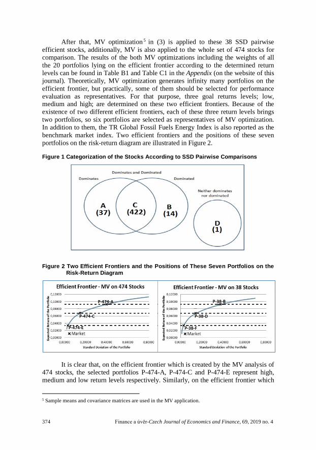
Following the examination of these 112101 pairwise SSD comparisons 4 according to (7), categorization of 474 stocks according to the SSD pairwise comparisons can be found in Figure 1. Obviously, the SSD pairwise efficient set includes 38 stocks which belong to clusters A and D.

3 It is obvious that the constituent stocks of the Thomson Reuters (TR) Global Fossil Fuels Energy Index is dynamic, thus it must be underlined that the list of 606 stocks are obtained at 22.01.2015. Although the common practice is to take all the changes of the index into account in the finance literature (see e.g. Gomez-Bezares et al., 2012), it is not relevant for this research to take the changing components of the index into account in this paper. For this research, it is required that all the stocks have returns for all the observations. It is essential to perform SSD application, which is discussed in Section 2. Then, MV efficient portfolios are selected from the SSD-eliminated stocks and back-testing is performed on these portfolios. It means that the selected portfolios are followed in 2.5 years timeframe from the beginning to the end of the back-testing period. Applying a dynamic framework would cause to new portfolios and new applications for all the new periods. It would be also impossible to compare the results of these applications with each other due to changing portfolios. Therefore, it is not relevant to use a dynamic framework in that kind of analysis. Analysis of different time frames with the same or different data could always be thought as a further research idea. 4 As a prior step of pairwise SSD efficiency, pairwise FSD efficiency is also tested by using (6) for these 474 stocks. But according to FSD there cannot be found any FSD inefficient stock, in other words, FSD does not eliminate any inefficient stock. But, in the light of previous empirical works about this subject this result is not interesting since FSD is a much stronger comparison tool rather than SSD.


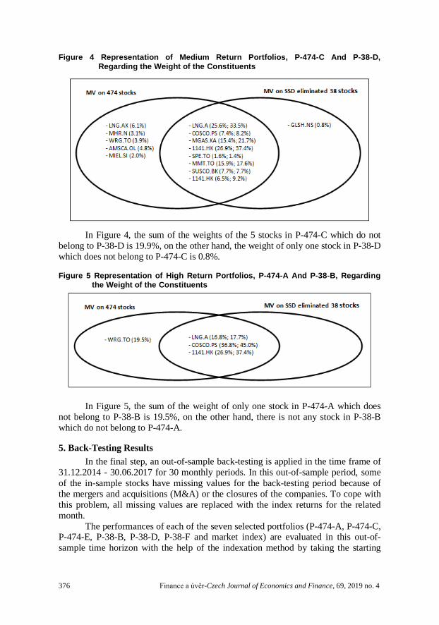
After that, MV optimization 5 in (3) is applied to these 38 SSD pairwise efficient stocks, additionally, MV is also applied to the whole set of 474 stocks for comparison. The results of the both MV optimizations including the weights of all the 20 portfolios lying on the efficient frontier according to the determined return levels can be found in Table B1 and Table C1 in the Appendix (on the website of this journal). Theoretically, MV optimization generates infinity many portfolios on the efficient frontier, but practically, some of them should be selected for performance evaluation as representatives. For that purpose, three goal returns levels; low, medium and high; are determined on these two efficient frontiers. Because of the existence of two different efficient frontiers, each of these three return levels brings two portfolios, so six portfolios are selected as representatives of MV optimization. In addition to them, the TR Global Fossil Fuels Energy Index is also reported as the benchmark market index. Two efficient frontiers and the positions of these seven portfolios on the risk-return diagram are illustrated in Figure 2.

Figure 1 Categorization of the Stocks According to SSD Pairwise Comparisons

Figure 2 Two Efficient Frontiers and the Positions of These Seven Portfolios on the Risk-Return Diagram

It is clear that, on the efficient frontier which is created by the MV analysis of 474 stocks, the selected portfolios P-474-A, P-474-C and P-474-E represent high, medium and low return levels respectively. Similarly, on the efficient frontier which

5 Sample means and covariance matrices are used in the MV application.


is created by the MV analysis of 38 SSD pairwise efficient stocks; P-38-B, P-38-D and P-38-F are correspondents of P-474-A, P-474-C and P-474-E on the same return levels.

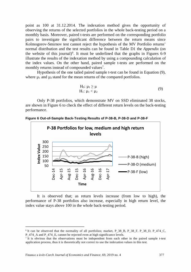
Figure 3, 4 and 5 display the weights of these six portfolios’ constituents, classified by the return level of the investor; low, medium and high; respectively. In these Venn diagrams, the percentage in parenthesis shows the weight of the stock in the related portfolio; obviously, the stocks in the intersection area belong to both portfolios. The first percentage in the parenthesis represents the weight in “MV on 474 Stocks” and similarly second one illustrates the weight in “MV on SSD eliminated 38 Stocks”.

Figure 3 Representation of Low Return Portfolios, P-474-E And P-38-F, Regarding the Weight of the Constituents

In Figure 3, the sum of the weights of the 13 stocks in P-474-E which do not belong to P-38-F is 40.1%, on the other hand, the sum of the weights of the 3 stocks in P-38-F which do not belong to P-474-E is 13.8%.


Figure 4 Representation of Medium Return Portfolios, P-474-C And P-38-D, Regarding the Weight of the Constituents

In Figure 4, the sum of the weights of the 5 stocks in P-474-C which do not

belong to P-38-D is 19.9%, on the other hand, the weight of only one stock in P-38-D which does not belong to P-474-C is 0.8%.

Figure 5 Representation of High Return Portfolios, P-474-A And P-38-B, Regarding the Weight of the Constituents

In Figure 5, the sum of the weight of only one stock in P-474-A which does not belong to P-38-B is 19.5%, on the other hand, there is not any stock in P-38-B which do not belong to P-474-A.

5. Back-Testing Results In the final step, an out-of-sample back-testing is applied in the time frame of

31.12.2014 - 30.06.2017 for 30 monthly periods. In this out-of-sample period, some of the in-sample stocks have missing values for the back-testing period because of the mergers and acquisitions (M&A) or the closures of the companies. To cope with this problem, all missing values are replaced with the index returns for the related month.

The performances of each of the seven selected portfolios (P-474-A, P-474-C, P-474-E, P-38-B, P-38-D, P-38-F and market index) are evaluated in this out-of-sample time horizon with the help of the indexation method by taking the starting


point as 100 at 31.12.2014. The indexation method gives the opportunity of observing the returns of the selected portfolios in the whole back-testing period on a monthly basis. Moreover, paired t-tests are performed on the corresponding portfolio pairs to investigate the significant difference between the return means since Kolmogorov-Smirnov test cannot reject the hypothesis of the MV Portfolio returns’ normal distribution and the test results can be found in Table D1 the Appendix (on the website of this journal)6. It must be underlined that the graphs in Figures 6-9 illustrate the results of the indexation method by using a compounding calculation of the index values. On the other hand, paired sample t-tests are performed on the monthly returns instead of compounded values7.

Hypothesis of the one tailed paired sample t-test can be found in Equation (9), where µ1 and µ2 stand for the mean returns of the compared portfolios.

H0: µ1 ≥ µ H1: µ1 < µ2

(9)

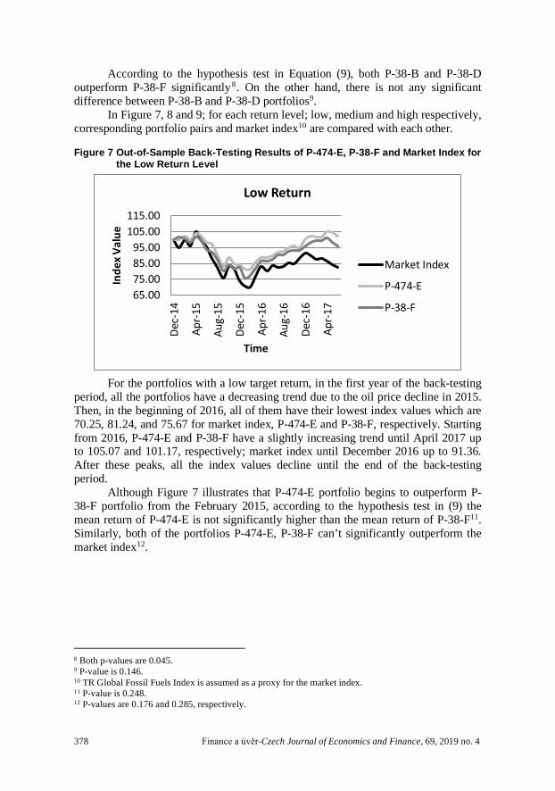
Only P-38 portfolios, which demonstrate MV on SSD eliminated 38 stocks,

are shown in Figure 6 to check the effect of different return levels on the back-testing performance.

Figure 6 Out-of-Sample Back-Testing Results of P-38-B, P-38-D and P-38-F

It is observed that; as return levels increase (from low to high), the

performance of P-38 portfolios also increase, especially in high return level, the index value stays above 100 in the whole back-testing period.

6 It can be observed that the normality of all portfolios; market, P_38_B, P_38_F, P_38_D, P_474_C, P_474_A and P_474_E, cannot be rejected even at high significance levels. 7 It is obvious that the observations must be independent from each other in the paired sample t-test application process, thus it is theoretically not correct to use the indexation values in this test.

50100150200250300

Dec-

14

Apr-

15

Aug-

15

Dec-

15

Apr-

16

Aug-

16

Dec-

16

Apr-

17

Inde

x Va

lue

Time

P-38 Portfolios for low, medium and high return levels

P-38-B (high)

P-38-D (medium)

P-38-F (low)


According to the hypothesis test in Equation (9), both P-38-B and P-38-D outperform P-38-F significantly8. On the other hand, there is not any significant difference between P-38-B and P-38-D portfolios9.

In Figure 7, 8 and 9; for each return level; low, medium and high respectively, corresponding portfolio pairs and market index10 are compared with each other.

Figure 7 Out-of-Sample Back-Testing Results of P-474-E, P-38-F and Market Index for the Low Return Level

For the portfolios with a low target return, in the first year of the back-testing

period, all the portfolios have a decreasing trend due to the oil price decline in 2015. Then, in the beginning of 2016, all of them have their lowest index values which are 70.25, 81.24, and 75.67 for market index, P-474-E and P-38-F, respectively. Starting from 2016, P-474-E and P-38-F have a slightly increasing trend until April 2017 up to 105.07 and 101.17, respectively; market index until December 2016 up to 91.36. After these peaks, all the index values decline until the end of the back-testing period.

Although Figure 7 illustrates that P-474-E portfolio begins to outperform P-38-F portfolio from the February 2015, according to the hypothesis test in (9) the mean return of P-474-E is not significantly higher than the mean return of P-38-F11. Similarly, both of the portfolios P-474-E, P-38-F can’t significantly outperform the market index12.

8 Both p-values are 0.045. 9 P-value is 0.146. 10 TR Global Fossil Fuels Index is assumed as a proxy for the market index. 11 P-value is 0.248. 12 P-values are 0.176 and 0.285, respectively.

65.0075.0085.0095.00

105.00115.00

Dec-

14

Apr-

15

Aug-

15

Dec-

15

Apr-

16

Aug-

16

Dec-

16

Apr-

17

Inde

x Va

lue

Time

Low Return

Market Index

P-474-E

P-38-F


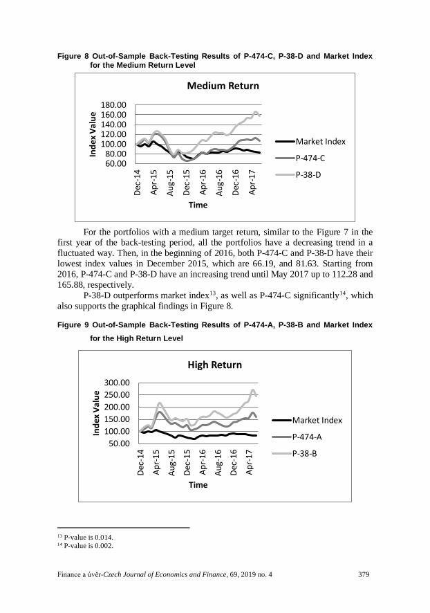
Figure 8 Out-of-Sample Back-Testing Results of P-474-C, P-38-D and Market Index for the Medium Return Level

For the portfolios with a medium target return, similar to the Figure 7 in the

first year of the back-testing period, all the portfolios have a decreasing trend in a fluctuated way. Then, in the beginning of 2016, both P-474-C and P-38-D have their lowest index values in December 2015, which are 66.19, and 81.63. Starting from 2016, P-474-C and P-38-D have an increasing trend until May 2017 up to 112.28 and 165.88, respectively.

P-38-D outperforms market index13, as well as P-474-C significantly14, which also supports the graphical findings in Figure 8.

Figure 9 Out-of-Sample Back-Testing Results of P-474-A, P-38-B and Market Index for the High Return Level

13 P-value is 0.014. 14 P-value is 0.002.

60.0080.00

100.00120.00140.00160.00180.00

Dec-

14

Apr-

15

Aug-

15

Dec-

15

Apr-

16

Aug-

16

Dec-

16

Apr-

17

Inde

x Va

lue

Time

Medium Return

Market Index

P-474-C

P-38-D

50.00100.00150.00200.00250.00300.00

Dec-

14

Apr-

15

Aug-

15

Dec-

15

Apr-

16

Aug-

16

Dec-

16

Apr-

17

Inde

x Va

lue

Time

High Return

Market Index

P-474-A

P-38-B


For the portfolios with a high target return, both portfolios P-474-A and P-38-B have a peak in May 2015, with the values of 180.60 and 216.81, respectively. After this point, both series have a fluctuated decreasing trend until January 2016 down to 106.95 and 125.01, respectively. It is observed that there is a sharp increase from the beginning of 2016 until May 2017. Indexation values reach the levels of 177.59 for P-474-A and 271.33 for P-38-B, which means that the P-38-B portfolio brings the initial investment to its 2.7 fold in less than 2.5 years from January 2015 to May 2017.

Similar to the finding of medium target return; P-38-B outperforms market index 15 , as well as P-474-A significantly 16 , which also supports the graphical findings in Figure 9.

6. Conclusions In this paper, an SSD pre-elimination method is added to classical MV

optimization and this two-step method is applied in the energy sector. Afterwards, the performance of the selected portfolios is measured by an out-of-sample back-testing. This paper has a common denominator with the previous works of Fulga et al. (2009), Kopa and Tichy (2014) and Lean et al. (2015) since it develops MV optimization by combining it with different methods. Additionally, this paper also applies the back-testing method to evaluate the performance of the selected portfolios in accordance with the studies of Roman et al. (2013), Tas et al. (2015) and Tas et al. (2016). Lastly, this paper can be considered as an extension of the research Guran and Tas (2015) since it uses SSD pre-elimination before MV optimization, but apart from Guran and Tas (2015), this paper applies a comprehensive back-testing performance evaluation, which is supported by paired sample t-test on monthly returns, dependent on the return and risk levels of the investors compared with the market index.

Since this paper adopts an expanding MV analysis it is clear that the interpretation of the results is intensively dependent on the return-risk level of the portfolios lying on the efficient frontier. Thus, the success of the SSD pre-elimination method is also directly related to this dependency. As Figure 6 displays explicitly, in the field of energy the out of sample performance of the portfolios increases while its return-risk level rises, so that the portfolios of medium and high return level (P-38-D and P-38-B respectively) outperform the low return portfolio P-38-F also in statistical terms significantly.

Under the light of this point of view, the contribution of the applied SSD pre-elimination method should be examined only at these medium and high return-risk levels but not at the low return-risk level. Figure 8 and 9 display the superiority of the SSD pre-elimination extension very obviously, so that in both comparisons, P-38 portfolios, which are built with the help of the suggested SSD pre-elimination method, outperform the classical MV optimized P-474 portfolios according to paired sample t-test results, in statistical significant terms.

In short, the contribution of this paper is that the suggested SSD pre-elimination method changes the structure of the classical MV optimized portfolios by

15 P-value is 0.033. 16 P-value is 0.016.


eliminating the SSD inefficient stocks in the first step, so that these modified portfolios show higher performance than the original ones. At this point it should be also underlined that this success is limited to some portfolios of the efficient frontier where MV’s back testing performance is well17. In plain words, the suggested SSD pre-elimination method increases the success of some of the selected MV optimized portfolios on the efficient frontier which stand out with a better back-testing performance.

For a further research, this hybrid method can be re-applied in different conditions; such as changing the time periods of both analysis and back-testing, using different data frequencies instead of monthly, choosing other indexes or sectors. Additionally, an application, which allows short-selling case, could be an interesting research idea. Furthermore, as a recently improving research area (Post and Kopa (2013, 2017), Levy (2016)) third order stochastic dominance (TSD) which is valid for “not only risk averse but also skew-lover” investors, can also be applied as a further step of SSD.

17 Specially in the field of energy, which is analysed in this paper, these more successful regions of the efficient frontier occurred in upper parts, such as medium and high return-risk levels, but it must not be forgotten that this situation cannot be generalized to all sectors because of the dependency on the market.


REFERENCES

Athayde GM, Flores RG (2000): Introducing Higher Moments in CAPM. In: Dunis CL (eds): Advances in Quantitative Asset Management. New York: Springer Science+Business Media. Best RJ, Best RW, Yoder JA (2000): Value Stocks and Market Efficiency. Journal of Economics and Finance, 24(1):28-35. Branda M, Kopa M (2012): DEA-Risk Efficiency and Stochastic Dominance Efficiency of Stock Indexes. Czech Journal of Economics and Finance, 62(2):106-124. Branda M, Kopa M (2014): On Relations Between DEA-Risk Models and Stochastic Dominance Efficiency Tests. Central European Journal of Operations Research, 22(1),13-35. Brodie J, De Mol C, Daubechies I, Giannone D, Loris I (2009): Sparse and stable Markowitz portfolios. Proceedings of the National Academy of Sciences, 106(30):12267-12272. Bruni R, Cesarone F, Scozzari A, Tardella F (2017): On Exact and Approximate Stochastic Dominance Strategies for Portfolio Selection. European Journal of Operational Research 259(1):322-329. Delarue E, De Jonghe C, Belmans R, D'haeseleer W (2011): Applying Portfolio Theory to the Electricity Sector: Energy Versus Power. Energy Economics, 33(1):2-23. Dittmar R (2002): Nonlinear Asset Kernels Kurtosis Preference and Evidence from Cross Section of Equity Returns. Journal of Finance, 57:369-403. Dupačová J, Hurt J, Štěpán J (2002): Stochastic Modeling in Economics and Finance, Kluwer, Dordrecht. Elton E J, Gruber M J (1997): Modern Portfolio Theory, 1950 To Date. Journal of Banking & Finance, 21:1743-1759. Fang H, Lai T (1997): Co-Kurtosis and Capital Asset Pricing. Financial Review, 32:293–307. Fong WM (2009): Speculative Trading and Stock Returns: A Stochastic Dominance Analysis of the Chinese A-Share Market. Journal of International Financial Markets, Institutions & Money, 19:712-727. Fulga C, Dedu S, Serban F (2009): Portfolio Optimization with Prior Stock Selection. Economic Computation and Economic Cybernetics Studies and Research, 43(4):157-171. Gatfaoui H (2019): Diversifying Portfolios of U.S. Stocks with Crude Oil and Natural Gas: A Regime-Dependent Optimization with Several Risk Measures. Energy Economics, 80:132-152. Ghodrati H, Abbasi M (2014): An Application of Markowitz Theorem on Tehran Stock Exchange. Management Science Letters, 4(5):899-904. Gokgoz F, Atmaca M E (2012): Financial Optimization in the Turkish Electricity Market: Markowitz's Mean-Variance Approach. Renewable and Sustainable Energy Reviews, 16(1):357-368. Guran CB, Tas O (2015): Making Second Order Stochastic Dominance Inefficient Mean Variance Portfolio efficient: Application in Turkish BIST-30 Index. Iktisat Isletme ve Finans, 30(348):69-94. Gómez-Bezares F, Ferruz L, Vargas M (2012): Can We Beat the Market with Beta? An Intuitive Test of the CAPM. Spanish Journal of Finance and Accounting/Revista Española de Financiación y Contabilidad, 41(155):333-352. Kopa M, Tichy T (2014): Comparison of Mean-Risk Efficient Portfolios in Asia-Pacific Capital Markets. Emerging Markets Finance and Trade, 50(1):226-240. Kraus A, Litzenberger R H (1976): Skewness Preference and the Valuation of Risky Assets. Journal of Finance, 31:1085-1099. Kuosmanen T (2004): Efficient diversification according to stochastic dominance criteria. Management Science, 50(10), 1390–1406. Lean H H, McAleer M, Wong W (2015): Preferences of Risk-Averse and Risk-Seeking Investors for Oil Spot and Futures Before, During and After the Global Financial Crisis. International Review of Economics & Finance, 40:204-216.


Levy H (2016): Stocastic Dominance: Investment Decision Making under Uncertainty. Third edition. Springer Science, New York. Mansini R, Ogryczak W, Speranza MG (2015): Linear and mixed integer programming for portfolio optimization. EURO: The Association of European Operational Research Societies, Cham, Springer, Switzerland. Markowitz H M (1952): Portfolio Selection. The Journal of Finance, 7(1):77–91. Markowitz H M (1959): Portfolio Selection. Efficient Diversification of Investments. John Wiley&Sons, New York. Marrero GA, Puch LA, Ramos-Real FJ (2015): Mean-Variance Portfolio Methods for Energy Policy Risk Management. International Review of Economics&Finance, 40:246-264. Merton RC (1972): An analytic derivation of the efficient portfolio frontier. Journal of Financial and Quantitative Analysis, 7, 1851-1872. Rockafellar RT, Uryasev S, Zabarankin M (2006): Generalized Deviations in Risk Analysis. Finance and Stochastics, 10:51-74. Sirucek M, Kren L (2015): Application of Markowitz Portfolio Theory by Building Optimal Portfolio on the US Stock Market. Acta Universitatis Agriculturae et Silviculturae Mendelianae Brunensis, 63(4):1375-1386. Post T, Kopa M (2013): General Linear Formulations of Stochastic Dominance Criteria, European Journal of Operational Research, 230(2)321–332. Post T, Kopa M (2017): Portfolio Choice based on Third-degree Stochastic Dominance, Management Science, 63(10):3381 –3392. Post T, Vlient PV, Levy H (2008): Risk Aversion and Skewness Preference. A Comment. Journal of Banking and Finance, 32:1178-1187. Roman D, Mitra G, Zviarovich V (2013): Enhanced Indexation Based on Second Order Stochastic Dominance. European Journal of Operational Research, 228(1):273-281. Roques FA, Newbery DM, Nuttall WJ (2008): Fuel Mix Diversification Incentives in Liberalized Electricity Markets: A Mean–Variance Portfolio Theory Approach. Energy Economics, 30(4):1831-1849. Tas O, Barjiough FM, Ugurlu U (2015): A Test of Second Order Stochastic Dominance with Different Weighting Methods: Evidence from BIST-30 and DJIA. Journal of Business Economics and Finance, 4(4):723-731. Tas O, Tokmakcioglu K, Ugurlu U, Isiker M (2016): Comparison of Ethical and Conventional Portfolios with Second-Order Stochastic Dominance Efficiency Test. International Journal of Islamic and Middle Eastern Finance and Management, 9(4):492-511. Ugurlu U, Tas O, Guran CB, Guran A (2018): SSD Efficiency at Multiple Data Frequencies: Application on the OECD Country Indexes. Prague Economic Papers, 27(2):169-195. U.S. Energy Information Administration (2016): International Energy Outlook 2013. Retrieved from: http://www.eia.gov/forecasts/ieo/pdf/0484(2013).pdf (2013). Accessed on 8 April 2018. Wong W (2007): Stochastic Dominance and Mean–Variance Measures of Profit and Loss for Business Planning and Investment. European Journal of Operational Research, 182:829–843. Yitzhaki S, Mayshar J (2001): Characterizing Efficient Portfolios. Available at SSRN 297899.

http://www.eia.gov/forecasts/ieo/pdf/0484(2013).pdf

mean-variance portfolio optimization f energy o stocks

Documents