IFS Means-testing and tax rates on earnings Mike Brewer Emmanuel Saez Andrew Shephard

Prepared for the Report of a Commission on Reforming the Tax System for the 21st Century, Chaired by Sir James Mirrlees

www.ifs.org.uk/mirrleesreview

The Institute for Fiscal Studies Full Report to be published by Oxford University Press

Means-testing and tax rates on earnings∗

Mike Brewer, IFSEmmanuel Saez, UC Berkeley

Andrew Shephard, UCL and IFS

April 8, 2008

∗This paper has been prepared for the Mirrlees Review - Reforming the Tax System for the 21st Century,http://www.ifs.org.uk/mirrleesreview/. Mike Brewer, Institute for Fiscal Studies, mike b@ifs.org.uk,Emmanuel Saez, saez@econ.berkeley.edu, University of California, Department of Economics, 549 EvansHall #3880, Berkeley, CA 94720, Andrew Shephard, Institute for Fiscal Studies, andrew s@ifs.org.uk. Wethank Stuart Adam, Tony Atkinson, Kate Bell, Richard Blundell, Hilary Hoynes, Paul Johnson, Guy Laroque,Costas Meghir, James Mirrlees, Robert Moffitt, James Poterba and numerous conference participants for helpfulcomments and discussions. Saez acknowledges financial support from the National Science Foundation grantSES-0134946. The Survey of Personal Incomes, the Labour Force Survey, and Family Expenditure Survey, theFamily Resources Survey and the General Household Survey datasets are crown copyright material, and arereproduced with the permission of the Controller of HMSO and the Queen’s Printer for Scotland. The SPI,LFS and GHS data-sets were obtained from the UK Data Archive, and FRS from the Department for Workand Pensions, and the FES from the Office for National Statistics. None of these government department northe UK Data Archive bears any responsibility for their further analysis or interpretation.

1 Summary and key findings

The setting of income tax rates and the generosity and structure of income support programmes

generate substantial controversy among policy-makers and economists. At the centre is a trade-

off between the goals of equity and efficiency: governments want to transfer resources from

the rich to the poor; on the other hand, such transfers reduce people’s incentive to work.

The key insight from the standard “optimal income tax model” developed by James Mir-

rlees is that marginal rates of tax and benefit withdrawal should be higher when people’s

choices of how much to work are relatively unresponsive to them and when the government

is relatively keen to redistribute resources from rich to poor. Furthermore, the government

should apply high marginal rates at points in the earnings distribution where there are few

taxpayers relative to the number of taxpayers who have earnings exceeding this amount. Using

data on the UK earnings distribution, we show that the optimal structure of marginal rates

in this simplified model has a U-shaped pattern, with high marginal rates imposed on high

and low earners and lower marginal rates on those in the middle. We show how this structure

changes as both the assumed responsiveness of hours of work and the government’s assumed

preferences for redistribution vary.

The way that incomes have responded to the large changes in top marginal tax rates

over the past 40 years suggests that if the richest 1% see a 1% fall in the proportion of each

additional pound of earnings that is left after tax, then the income they report will rise by less

than half that - only 0.46%. Although a tentative estimate, this suggests that the government

would maximise the revenue it collects by imposing an overall marginal rate on the highest

earners of 56.6%, very close to the 53.0?% currently charged in the UK (including income tax,

national insurance contributions and indirect taxes). So there does not seem a powerful case

for increasing the income tax rate on the very highest earners, even on redistributive grounds

– it would not generate much if any extra revenue to transfer to the less well off.

When the optimal tax model is enriched by allowing individuals to respond to taxes and

benefits by deciding whether or not to work, as well as how hard, then the optimal structure

of marginal rates changes dramatically. In particular, when the decision whether to work

becomes relatively more important to the decision about how much to work, then marginal

rates and the proportion of gross income taken in tax and withdrawn benefits when people

1

enter work should be set low (and perhaps even negative) for potential low earners rather than

set high as the standard model suggests. We also discuss how the design of taxes and benefits

affecting an individual should be affected by the presence of a co-resident partner or dependent

children, although it is difficult to reach definitive conclusions. We argue that the practical

operation of benefits and tax credits for low-income families is important and that they would

be of greatest help to beneficiaries if they were assessed over short periods and paid promptly

without retrospective adjustment.

These insights from optimal tax theory are contrasted with the work incentives inherent

in the current UK tax and benefit system. Four key deficiencies are identified:

1. The amount of gross income taken in tax and withdrawn benefits when people enter

work at low earnings is too high: for most groups it is close to 100% before individuals

are entitled to the working tax credit, and they remain high even with it.

2. The marginal rate of 73.4% that many low to moderate earners face when having tax

credits withdrawn is likely to be above the optimum rate even if people’s decision to

work a little harder is relatively unresponsive.

3. Housing Benefit, the main means-tested programme though which the government helps

people on relatively low incomes with their housing costs has an extremely high with-

drawal rate. This exacerbates the problem of undesirably high marginal rates. It is also

hard to administer and is not claimed by many working families entitled to it.

4. While the system for administering income tax and national insurance contributions in

the UK is simple and efficient, tax credits, housing benefit and council tax benefit are all

burdensome to claim, relatively expensive for the government to administer, and prone

to significant fraud and error.

Given this diagnosis, we suggest a set of changes to the existing tax and benefit structure

that could be made immediately based on the lessons from our analysis. Our package of

”immediate reforms” involves:

• Increasing the amount people can earn before they have means-tested benefits withdrawn.

This would increase the financial gain to entering work at low earnings;

2

• Increasing the amount that second earners can earn before a family’s tax credits are

withdrawn. This would improve the financial incentive for a second earner to enter

work, especially if they have children;

• Reducing the rate at which child and working tax credits are withdrawn with every extra

pound earned;

• Targeting increases in working tax credit on groups other than lone parents.

This would cost around £9 billion per year. If it had to be financed from within the income

tax and benefit system, the money could be raised by cutting child benefit and/or increasing

the basic rate of income tax. Neither would undo the objectives of the reform package to

improve work incentives, although both would pose big political challenges.

We also suggest a more radical and comprehensive plan for reforming the UK household tax

and benefit system that attempts to deal not only with these work incentive issues, but also the

administrative failings that we identify. Our plan replaces the existing piece-meal benefits for

low-income families (income support, working and child tax credits, housing benefit and council

tax benefit) with a single Integrated Family Support (IFS) programme which provides stronger

and simpler incentives for work at the bottom, reduces compliance costs for families, and is

means-tested by employers’ withholding from earnings in the same way as National Insurance

contributions. We show how, after including an assessment of the behavioural responses, the

IFS manages to redistribute more income with minimal impact on total earnings and total net

tax revenue, by targeting net tax cuts where incentives to work are currently at their weakest.

2 Introduction

The setting of income tax rates, and the generosity and structure of income support (or trans-

fer) programmes generate substantial controversy among policy-makers and economists. At

the centre is an equity-efficiency trade-off. On the one hand, governments value redistribution,

and so want to transfer resources from the rich to the poor, usually by taxing the incomes of

the rich and subsidising the incomes of the poor. On the other hand, this redistribution is

generally costly in terms of economic efficiency because of the disincentive effects of taxes and

transfers (we explain this in more detail in section 3). The costs arise for two reasons : first,

3

raising income taxes may weaken the labour supply and entrepreneurship incentives of middle

and high income individuals who face the taxes. Second, income transfer programmes may

weaken the labour supply incentives of their recipients. These two responses can substantially

raise the cost of improving the living standards of low income families.

The goal of this chapter is to provide an overview of the way economists think about the

design of taxes and benefits affecting households, and to apply the lessons from this literature

to the design of the UK tax and benefit system.

In economics research, the problem of designing taxes and benefits is tackled in two steps.

The first step is a positive analysis, where economists develop models of individual behaviour

to understand how individuals’ work decisions respond to taxes and benefits. The central part

of the positive analysis is the empirical estimation of models of individual behaviour, and there

is a very broad literature that tries to estimate the size of the behavioral responses to taxes

and benefits.1

The second step is the normative analysis, or optimal policy analysis. Using models de-

veloped in the positive analysis, the normative analysis investigates what structure and size

of the tax and benefit system would best meet a given set of policy goals; following Mirrlees

(1971), economists call this line of research “optimal tax theory”. Despite its name, optimal

tax theory concerns itself just as much with the design of benefits as it does the setting of

income tax rates: one of the key concepts of optimal tax theory is that of a net tax function,

whereby people with high incomes pay some of that income in positive taxes to the govern-

ment, and people with a low income receive money from the government (by paying negative

taxes); no conceptual distinction is made between net recipients from and net contributors to

the state’s finances.2

At its heart, optimal tax theory says that the two desirable features of a tax and benefit

system are that it be fair, and that it minimise disincentive effects.3 But the problem of

having two desirable features is that one has to know how much weight to give to each. For

example, a poll tax (under which all individuals have to pay the same level of tax) might have1The way that these models are estimated, and the key insights, are summarised in Meghir and Phillips,

this volume.2One difference between the tax system and the transfer system is that the former is usually cheaper to

administer, and these distinctions can be reflected in more complicated optimal tax models.3More complicated models can allow for other desirable features: one might be that a tax and transfer

system is cheap to administer; Shaw et al, this volume, consider how this alters optimal tax models.

4

no disincentive effects, but is rather unfair to those on low incomes. As Heady (1993, p17)

says, “the approach of the optimal tax literature is to use economic analysis to combine these

criteria into one”. It does this by saying that the objective of the government when designing

the tax and benefit system should be to maximise social welfare (subject to a need to raise a

certain amount of revenue). Precisely how social welfare is expressed is not relevant at this

stage, but the idea is that it reflects in a single index (or number) the desire both to have the

economy as large as possible (because this directly increases people’s well-being) but also to

have the income distributed as equally as possible. The expression for social welfare precisely

quantifies the trade-off between these two desiderata: returning to the previous example of an

economy with only a poll-tax, replacing that with an income tax which raised the same amount

of money would give a more equal distribution of income, but - if there any disincentive effects

to taxation - a smaller economy.

The normative analysis is crucial for policy-making because it shows how taxes and benefits

should be designed in order to best attain the goals of the policy-maker. In particular, the

normative analysis allows one to assess separately how changes in the redistributive criterion

of the government, and changes in the size of the behavioural responses to taxes and transfers,

affect the optimal tax and benefit programme. Conversely, the normative analysis makes it

explicit that one cannot hope to say how best to design taxes and transfers without both

knowing how individuals will respond, and without specifying what one is trying to achieve

overall. Often, these two elements are confused in policy debates: right-of-centre policy-makers

rarely state explicitly that they have little taste for redistribution, but instead justify their

lack of taste for redistribution because they believe that the adverse behavioural responses to

high taxes or generous benefits are large. Conversely, left-of-centre policy-makers emphasize

the redistributive virtues of benefits and assume that adverse behavioural responses to these

and the high tax rates needed to fund them are negligible.

We provide this overview as follows: section 3 introduces the standard optimal tax model

developed in Mirrlees (1971). This shows directly how the the optimal tax and benefit system

is determined by both the social welfare criterion used by the government and the size of

behavioural responses to taxation. Despite the simplifications inherent in the model, we can

use it to analyse the optimal tax rate that should apply to top incomes, where we present new,

albeit tentative, evidence on the response of top incomes to the large changes in top marginal

5

tax rates that have taken place in the UK over the last 40 years. Section 4 extends the

optimal tax model to allow for labour supply participation effects, and shows that allowing for

such responses can drastically change the optimal tax system affecting low income individuals:

instead of traditional welfare programmes with high withdrawal rates, large in-work benefits

such as Working Tax Credit in the UK or the Earned Income Tax Credit from the US, which

can have very low or negative withdrawal rates, can be optimal.4 We also discuss the issue of

migration and tax design, which can be dealt with in optimal tax models in a similar manner

to the issue of labour market participation. Throughout Sections 3 and 4, we make use of the

summary of the literature on the behavioural response to taxation provided in Meghir and

Phillips, this volume.

In Section 5, we analyze a set of additional issues relevant to the design of the tax and

benefit system affecting households. First, we discuss how the family should be taxed: the

models considered in sections 3 and 4 abstract from family issues, but a majority of adults

in reality live in couples, and so can be assumed to pool income to some extent. We also

discuss how the presence of children should be reflected in the optimal tax design. Lastly,

we discuss administrative and operational issues concerning benefits.5 Section 6 describes

how the main elements of the current UK personal tax and benefit system affect incentives

to work and earn more and, in Section 7, we provide a critique of the UK tax and benefit

system, and set out the direction of reform suggested by the insights from optimal tax theory,

and the latest evidence on the behavioural response to taxation. To crystallise ideas, we

propose specific changes that could be implemented in the short-run. But most optimal tax

theory uses simplified models which leave aside a number of important practical issues such

as administrative burden for the government and employers, and ease of use for families.6

Those issues have always been important in practice, and the recent “behavioral economics”

literature is starting to incorporate them in the analysis. Therefore, we go further and propose

a longer-term reform that builds on the short-run changes to incentives by addressing the main

practical issues with the current benefits in the UK. Our plan replaces the piece-meal benefits

for low-income families (income support, working and child tax credits, housing benefit and4To anticipate our discussion in section 5, the WTC can lead to negative PTRs, but not negative METRs,

whereas the EITC can lead to negative METRs as well.5Shaw et al, this volume, discusses administrative and operational issues affecting tax design.6A number of those issues are discussed in more detail in the chapter by Shaw et al, this volume.

6

council tax benefit) into a single Integrated Family Support programme which provides stronger

and simpler incentives for work at the bottom, reduces compliance costs for families, and is

provided “as-you-earn” and administered in the same way as social contributions through the

PAYE withholding system.We show how this can be done in a revenue-neutral fashion, and

estimate the behavioural responses to such a reform.

3 The standard optimal income tax model with intensive re-sponses

This section presents the standard model of optimal income tax, based on Mirrlees (1971), in

which individuals respond to the tax and benefit system by choosing only how much to work.

We then give two applications of the model to the UK:

• first, we can derive an expression for the optimal top marginal tax rate (ie, the marginal

tax rate facing the highest income individuals), and we go on to calculate this using new,

albeit tentative, evidence on the responsiveness of top incomes in the UK to changes in

top marginal tax rates over the last 40 years.

• second, we simulate the entire optimal tax system for the UK given some various highly

simplifying assumptions in order to show how the optimal tax system is determined by

both the social welfare criterion used by the government, and the size of behavioural

responses to taxation.

Before that, though, section 3.1 sets out some of the key terms which will occur throught

this chapter.

3.1 Key concepts

3.1.1 The budget constraint, PTRs and METRs

A useful tool to investigate the disincentive effects of taxes and transfers is the budget con-

straint.7 This shows the relationship between gross earnings (or hours of work) and net income

after taxes and transfers, and an example is given in Figure 1A (the example is for a lone par-

ent with 2 children, and we discuss this Figure in more detail and look at other family types

in section 6).7This draws on chapter 2 of Adam et al (2006).

7

The budget constraint contains all the information we need to know about how taxes and

transfers affect financial incentives to work, but in this chapter we frequently refer to some

summary measures of work incentives:

• the participation tax rate (PTR) is defined as 1 minus the financial gain to work as

a proportion of gross earnings. It measures how the tax and benefit system affect the

financial gain to work. If someone who did not work had an income from a benefit

programme of £60 a week, and would earn £250 in gross earnings, but pay £40 of that

in income tax if they were to work, then the PTR is given by 1 - (210-60)/250, or 40%.

The higher the number, the more the tax and benefit system reduces the financial gain

to work. A PTR in excess of 1 means the individual would be worse off in work then not

working; a PTR equal to 1 means that there is no financial reward to work; a PTR of

zero means that the financial reward to work is equal to gross earnings; negative PTRs

are possible where benefits are conditional on being in work or having positive earnings.

• the marginal effective tax rate (METR) measures how much of a small rise in gross

earnings is lost to payments of tax and reduced entitlements to benefits. It is equal

to the slope of the budget constraint at any particular point. The higher the number,

the more the tax and benefit system reduces the gain to earning a bit more: a METR

in excess of 1 means that an individual would be worse off if they earned a bit more;

a METR of 1 means that an individual would be unaffected by any small change in

earnings; a METR of zero means that the individual is keeping all of any small rise

in earnings; and a negative METR means that an individual’s net income increases by

more than a small change in earnings (this can arise where benefits act as a proportional

subsidy on earnings, such as the phase-in portion of the earned income tax credit in the

US).

• It is sometimes more useful to consider the net-of-tax rate, or one minus the METR: this

measures how much work pays at the margin.

Figure 1B shows how the schedule of PTRs and METRs for the example budget constraint

in Figure 1A; we discuss the particular features of this budget constraint in section 6.

8

3.1.2 Labour supply responses to taxation

Economists think about the disincentive effects of the tax and benefit system using a labour

supply model.8A basic labour supply model assumes that, when deciding whether and how

much to work, people trade off the financial reward to working (plus any intrinsic benefits

from working) with the loss of leisure time (by ”work” we mean ”participate in the labour

market”, rather than doing unpaid work at home or elsewhere).

As we discussed above, taxes and transfers affect labour supply because they alter the finan-

cial reward to working, both by making the net wage lower than the gross wage (most taxes,

some transfers) and by reducing the financial gain from working compared to not working

(most transfers). Economists usually distinguish between two ways that financial considera-

tions affect labour supply:9

1. the impact of the METR on labour supply is called the substitution effect, as increasing

the METR (thereby reducing the net-of-tax rate) may lead individuals to work less,

or to substitute some leisure for work. Economists often measure this effect using the

elasticity of earnings with respect to the net-of-tax rate: this measures the percentage

increase in earnings following a one percent increase in the net-of-tax rate (see Box 1).

2. In addition, taxes and transfers may also affect labour supply through income effects:

higher taxes or cuts in benefits reduce the income available to individuals, and so may

induce individuals to work more in order to increase their standard of living. Equally,

lower taxes or more generous benefits increase income, and hence may induce individuals

to work less. Because the derivation of optimal income tax models is much simpler when

there are no income effects (Diamond, 1998 and Saez, 2001), we will assume no income

effects in the analysis below, and discuss later informally how the main results change

when there are income effects.8See Meghir and Phillips, this volume, and references therein, for more detail.9Meghir and Phillips, this volume, shows the different impacts graphically.

9

Box 1. The elasticity of earnings

We denote the marginal effective tax rate by τ so that the net-of-tax rate isgiven by 1 − τ . The elasticity of earnings z with respect to the net-of-tax rate1− τ is defined as:

e =1− τz

∂z

∂(1− τ).

This elasticity e is always positive. The higher is e, the more responsive areearnings to the net-of-tax rate.

To give an example of its use, if e is 0.2, and the net of tax rate changes from20% to 25% (ie the METR falls from 80% to 75%), then earnings will rise by0.2 ∗ 5%

20% = 5%. If the net of tax rate changes from 80% to 75% (ie the METRrise from 20% to 25%), then earnings will fall by 0.2 ∗ 5%

80% = 1.25%

3.2 The Mirrlees model

In the Mirrlees model of optimal taxes, the government is trying to design a tax and benefit

system that will maximise social welfare and raise a given amount of revenue. Mirrlees (1971)

allowed the tax and benefit system to be non-linear, which means that METRs at a particular

point of the earnings distribution can be set to any value without altering METRs at other

points. The model assumes that people vary in their earnings potential (or what they would

earn if there were no taxes or transfers), and that everyone always works, but chooses how

much effort to supply (”effort” can be thought of as hours of work, with a given hourly wage

for each individual, but there are other interpretations, as we discuss later).

Before discussing how this model can be used to determine the optimal METR at any point

in the income distribution, we first show how it can be used to derive the optimal METR for

high-income individuals, a simpler task.

• The optimal top marginal tax rate

To determine the optimal top METR, we will consider the different ways in which a small

increase in the top METR affects social welfare. Some of these effects will be positive, and

others negative, but at the optimum they must be exactly offsetting, so that no small change

in the tax rate can better achieve the goals of the government.

We assume that this top METR applies to earnings above a given level, and we will refer

10

to this level as the top bracket.10 There are three impacts on social welfare:

1. With no behavioural response, increasing the top METR will increase government rev-

enue. This is the mechanical effect on tax revenue, and this is a benefit to society, as the

revenue can be used for government spending or higher transfers.

2. However, increasing the top METR may also induce top bracket taxpayers to reduce

their earnings (but not below the top bracket, because the budget constraint has not

changed below this point) because of the substitution effect described above. This is

known as the behavioural response on tax revenue, and it is a cost to society as tax

revenues will fall.

3. Finally, any increase in the top METR will reduce the welfare of top bracket taxpayers.

This is the welfare effect, and it is a loss to society. How large is this loss depends

on the redistributive tastes of the government: if the government values redistribution,

then, for incomes above a certain level, it will consider that the marginal value of income

for top-bracket tax-payers is small relative to the average person in the economy. In the

limit, the welfare effect will be negligible relative to the mechanical effect on tax revenue.

An optimal top METR is one where the marginal costs and benefits of increasing it further

are balanced. If the welfare effect is negligible, then the government should increase the top

METR up to the point where the mechanical increase in tax revenue is equal to the loss in

tax revenue from the behavioral response. This effectively amounts to setting the top METR

so as to maximize the tax revenue collected from top bracket taxpayers; this can therefore be

considered as an upper bound to the top METR above which no government should ever go.11

A precise formula for this optimum top METR is provided in Box 2. The more responsive

are earnings to the net-of-tax rate, and the thinner is the income distribution at the top (we

formalise this concept in Box 4), then the lower should be the top METR. Later in this section

3.2, we provide estimates for both these parameters for the UK.10As already noted, the current top rate of income tax in the UK is 40% and applies to annual earnings

greater than £41,435 (in 2008-9). When including National Insurance contributions, the marginal effective taxrate is 47.7% on top earnings.

11It is straightforward to extend the theory to the case where the government has less redistributive tastesand hence the welfare effect is not negligible. See e.g. Saez (2001) .

11

Box 2. Determining the top rate of income tax

Here we present the optimal marginal tax rate τ for high earners that maximizestax revenue. We denote by z the average income reported by taxpayers in thetop bracket (incomes above z). By balancing the mechanical and behaviouraleffects, the optimal rate τ∗ can be shown to be given by:

τ∗ =1

1 + a · e

where a denotes the ratio z/(z − z) and is a measure of the thinness of the topof the income distribution. The optimal rate is decreasing in both the elasticitye and the shape parameter a. See Appendix for derivation.

• Optimal marginal tax schedule

Using a similar technique to how we derived the optimal METR in the top bracket, we can

also derive the optimal METR at any point of the income distribution. As before, the optimal

METR at any point is set so as to balance the costs and benefits from changing the METR

by a very small amount.

As before, an increase in the METR over a very small band of income has three effects on

government tax receipts and welfare:

1. First, the reform increases taxes paid by every taxpayer with incomes above the small

band (the mechanical effect).

2. Second, the rise in the METR will reduce earnings for taxpayers in the very small band

through the substitution effect, and so generates a loss in tax revenue.

3. Third, the extra taxes paid by every taxpayer with incomes above the small band gen-

erates a welfare cost whose size will depend upon the extent to which the government

values redistribution.

For an optimal METR, these effects must exactly offset, so that no change in the tax

schedule can increase social welfare. An exact expression is presented in Box 3.

The key differences with this analysis and that in the previous section that looks at the

optimal top rate are:

• changing the METR at any point affects not just those facing that METR, but also all

those with higher earnings

12

• the welfare cost of extra taxes paid is no longer negligible.

Box 3. Determining the optimal marginal tax schedule

We assume that the government imposes a tax schedule T (z) that depends onearnings z. As shown in Figure 1A and 1B, the slope of this schedule, T ′(z),gives the METR when earnings are z. Let H(z) denote the the fraction of tax-payers with income less than z (ie cumulative distribution of individuals), andlet h(z) denote the density of taxpayers. The optimal tax system is character-ized by a grant to those with no earnings (equal to −T (0)) combined with aschedule of marginal tax rates T ′(z) which define first how the grant should bereduced as earnings increase, and then how additional earnings should be taxedonce the grant has been fully tapered away. The government’s preferences forredistribution are given by G(z) which measures the social marginal value ofconsumption for individuals with earnings above z (this should be decreasingin z if the government values redistribution). The optimal marginal tax rateT ′(z) is set so as to balance costs and benefits at the margin, and is given bythe following formula:

T ′(z)1− T ′(z)

=1e· 1−H(z)

zh(z)· (1−G(z))

The optimal tax rate T ′(z) is decreasing with the elasticity e, and decreasingin G(z), and increasing in the income distribution ratio (1 − H(z))/(zh(z))which measures the thinness of the earnings distribution. See Appendix formore details.

The formula in Box 3 shows how the optimal METR depends upon the size of the be-

havioural response to taxation, the government’s preferences for redistribution and the under-

lying shape of the (potential) earnings distribution. In particular, METRs should be higher:

• the less responsive are individuals to the net-of-tax rate

• the more value is placed on redistribution

• at points in the earnings distribution where the number of individuals is small relative

to the number of taxpayers with earnings exceeding this amount (this is because the

revenue gained from increasing METRs at a given earnings level will be proportional to

the number of individuals who have earnings greater than this level; the precise way that

we summarise this shape of the income distribution is discussed in Box 4).

13

Box 4. Summarising the shape of the income distribution

The shape of the income distribution is an important determinant of the optimalstructure of METRs. We summarise this shape by the income distribution ratio:

1−H(z)zh(z)

which appeared in the optimal taxation formula presented in Box 3 (where wesay that is measured the thinness of the income distribution). The optimalformula shows that the government should apply high marginal tax rates atlevels where the density of tax payers, measured by h(z , is low compared to thenumber of taxpayers with higher income, measured by 1−H(z).

To anticipate the discussion in section 3, it is worth noting that negative METRs are never

optimal: if the METR were negative in some range, then increasing it a little bit in that range

would raise revenue (and lower the earnings of taxpayers in that range), but the behavioural

response (which would be to work less) would also be to raise revenue, because the marginal

tax rate is negative in that range. Therefore, this small tax reform would unambiguously

increase social welfare.

Saez (2001) shows how the analysis changes when income effects are introduced. Income

effects encourage work for middle and upper income earners because taxes reduce disposable

income, but income effects discourage work for low-income earners, because transfers increase

disposable income. Hence income effects make taxing less costly, but make transfers more

costly. Therefore, holding other things constant, income effects lead to higher METRs at the

upper end, allowing the government to redistribute more, but make redistribution at the low

end more costly, and so the net effect on the level of transfers is ambiguous. If income effects

are concentrated at the bottom, then they are likely to reduce the size of the optimal transfers

at the bottom. If income effects are spread evenly throughout the distribution, then numerical

simulations by Saez (2001) show that income effects allow the government to increase the level

of transfers paid for by higher METRs across the distribution.

3.3 Empirical evidence on intensive elasticities, and applications to the UK

This section presents two applications of the results shown earlier to the UK tax system. We

first derive the optimal top METR, using new, albeit tentative, evidence on the responsiveness

of top incomes in the UK to changes in tax rates, based on the response of top incomes

14

to the large changes in METRs applying to top incomes that have taken place in the UK

over the last 40 years. We then derive the entire optimum tax schedule in the standard

intensive-responsive Mirrlees model, given assumptions for the labour supply elasticity and

the government’s preferences for redistribution.

• Top Incomes and the Optimal Top Tax Rate in the UK

Although there is a large literature analyzing the effects of changes in METRs on reported

incomes using tax return data in the US (see e.g., Saez, 2004 for a recent survey; some are

cited in Meghir and Phillips, this volume), there has been little study of the British case. This

is especially surprising, given that the UK experienced a dramatic drop in top METRs. Up to

1978, the top METR on earnings was 83% 12. Under the Thatcher administrations, the top

rate dropped to 60% in 1979, and then dropped further to 40% in 1988.13

In this section, we propose a very preliminary analysis of the link between top METRs and

top incomes, using and extending the top income share series constructed by Atkinson (2007).

Those series estimate the share of total personal income accruing to various upper income

groups such as the top decile (the top 10 percent), or the top percentile (the top 1 percent),

and so they measure how top incomes evolve relative to the average.14 We have computed the

average METR faced by various upper income groups from 1962 to present (in fact, there are

two METR series, one including income tax and employer and employee national insurance

contributions, and one that also includes the impact of consumption taxes, such as VAT and

excise duties.15

12The top rate on capital income was even higher and reached the extraordinary level of 98% from 1974 to1978, although, as we remarked earlier about the top rate on earned income of 83%, very few individuals hadtaxable incomes high enough to face this rate.

13Dilnot and Kell (1988) try to analyze this issue, but have only access to a single year of micro-tax returns,and rely on aggregate numbers for their time-series analysis. More recently, Blow and Preston (2002) haveused micro tax data for 1985 and 1995 to analyze responses to tax rates, but they focus exclusively on theself-employed, and do not look specifically at top incomes. Atkinson and Leigh (2004) have analyzed the linkbetween top income shares and the top statutory marginal tax rate in five English speaking countries includingthe UK but their study does not estimate effective marginal tax rates and does not focus specifically on the UKcase.

14The definition of income used by Atkinson (2007) (and therefore by us in this section) is close to the broadincome definition used in Gruber and Saez (2002), as it excludes capital gains and certain renumeration in kind.However, there are some inconsistencies over time: the most important is that the data represents familiesbefore 1990 and individuals after 1990, and we make an adjustment to the pre-1990 data to correct for that (seeonline appendix for details). Atkinson (2007, p89) also says that the series omits employees’ superannuationcontributions before 1985, and before 1975-76, the series is net of retirement annuity premiums, alimony andmaintenance payments, and allowable interest payments.

15The consumption tax rate is assumed to be uniform, and estimated using total consumption tax receipts.

15

Figure 2A displays the METRs (excluding and including consumption taxes) on earnings

faced by the top 1% (on the left axis), and the top 1% income share (on the right axis) from

1962 to 2003. It shows an increase in the METR from 1962 to 1978 followed by a dramatic

decline in the two key income tax reforms of 1979 and 1988. The top income share series shows

an erosion of the top 1% income share up to 1978, followed by sharp upturn starting exactly

when the top METR was reduced in 1979, suggesting that top income shares did respond

to the lower METR. From a long-term perspective, the top 1% income share doubled from

6% in 1978 to 12.6% in 2003 while the net-of-tax rate (one minus the METR) doubled from

1− .79 = 21% in 1978 to 1− .53 = 47% in 2003 (using the rates including consumption taxes).

If all the increase in top incomes (relative to the average) can be attributed to the reduction

in the METR, this would imply a substantial elasticity almost equal to one.16

Figure 2B displays the METR and income share of the next 4% (income earners between

the 95th and the 99th percentile). In contrast to the top 1%, the METR in 1978 is virtually

identical to the current METR: this illustrates that the Thatcher tax reforms cut the pro-

gressivity of the income tax within the top 1%, but had relatively small effects on those with

slightly lower incomes. However, the income share of the next 4% also shows a break in 1979:

the income share is roughly constant at around 12% before 1979, and then increases steadily

from 12% to 15% from 1979 to 2003 despite there being little change in the METR.

Two interpretations of this are possible. First, it could be argued that the change in high

incomes was not entirely due to the cuts in the METR, and may have been caused by other

reforms enacted by the Thatcher administration that were favourable to high incomes. In that

case, our previous estimate of 0.93 is biased upward. Second, it is conceivable that income

earners in the next 4% group were also motivated to work harder by the prospect of facing

much lower rates should they succeed in getting promoted and become part of the top 1% in

coming years.17 In that case, if a cut in the METR facing the top 1% stimulated incomes

These and other computations are described in an online appendix. The METR is an average of the METR onearned and unearned income weighted by the share of earned and unearned income in each group. Our METRsare also weighted by income within each group, as larger incomes have a proportionately larger contribution tothe total behavioral response of the income group (indeed, in the optimal top tax rate formula (1), one needsto use the elasticity weighted by income).

16These elasticities are calculated by computing e = (logS1 − logS0)/(log(1 − τ1) − log(1 − τ0)) whereS0 the top 1% income share before the reform, S1 the share before the reform, τ0 the marginal tax rate ofthe top 1% before the reform, and τ1 the rate after the reform.. In this case, the elasticity is estimated as:log(12.6/6.0)/ log((1− .79)/(1− .53)) = .93.

17Gentry and Hubbard (2004) have tried to estimate such effects in a model of entrepreneurship with US

16

below the top 1%, our estimate of 0.93 would understate the overall on government revenues.

We show more systematically in Table 1 how this data can be used to estimate the elasticity

of broad income with respect to the net-of-tax rate. The first 2 rows of Table 1 focus on the 2

key tax cuts of 1979 and 1988, and compare 1978 with 1981 and 1986 with 1989, respectively18.

Column (1) estimates the elasticity of top 1% incomes by calculating how the share of income

received by the richest 1% of individuals changes relative to the change in the METR that

this group was subject to. It shows positive, but not very large, elasticities of 0.34 and 0.26.

However, as we discussed above, the longer-run perspective suggests higher elasticities. Indeed,

the third and fourth rows compare years 1962 to 1978 (when METRs for the top 1% increased)

and years 1978 to 2003 (as we discussed above), and these comparisons imply substantially

higher elasticities of 0.61 and 0.93. Finally, the bottom row presents the coefficient of a simple

time-series regression of the income share of the top 1% on the METR. Rather than just

comparing the changes between two different years, this approach uses data over the entire

1978 to 2003 period, and suggests an elasticity of 0.73 (which is statistically significant).

In Column (2) we again calculate the elasticity estimates of top earners, but we exclude

consumption taxes from our measure of METR: this hardly changes the elasticity estimates

(because average consumption tax rates have changed by much less than the marginal rate of

income tax applying to top incomes).

The elasticities reported in columns (1) and (2) are unbiased estimates only if, absent the

tax change, the top 1% income share would have remained constant. As we explained above,

this assumption seems contradicted by the fact that the top 5-1% income share increased from

1978 to 2003 in spite of no change in METRs. If we assume that, absent the tax change, the

top 1% share would have increased as much as the top 5-1% share, we can calculate what

is referred to as a difference-in-differences estimate, which is presented in column (3) of the

table.19 These difference-in-differences (DiD) estimates are smaller for the long-term 1978-2003

comparison, and for the full time-series regression, although they remain substantial at 0.64

and 0.46 respectively. It is conceivable that, absent the tax change, the top 1% share would still

have increased more than the top 5-1% share, perhaps because the Thatcher administration

data.18We do not use 1990 because of the change from couple to individual tax filing which creates a small

discontinuity in the Atkinson series.19Those elasticity estimates are e = (logS1/S

c1− logS0/S

c1)/(log(1−τ1)/(1−τ c1 )− log(1−τ0)/(1−τ c0 )) where

Sc and τ c are the income share and marginal tax rate for the “control group” Top 5-1%.

17

implemented other policy changes favorable to top incomes, or because of structural changes

in the labour market and changes in the returns to human capital.

Table 1: Elasticity Estimates for Top Income Earners

Simple Difference Simple Difference DD using(excluding consumption Top 5-1% as

tax from MTR) control(1) (2) (3)

1978 vs. 1981 0.34 0.32 0.081986 vs. 1989 0.37 0.38 0.411978 vs. 1962 0.61 0.63 0.862003 vs. 1978 0.93 0.89 0.64

Full time-series 0.73 0.69 0.46regression (0.13) (0.12) (0.13)(s.e. in brackets)

The second parameter in formula (1) is a, the measure of the thinness of the income

distribution at the top (see Box 4). Figure 3 shows how our measure of the shape of the

income distribution (discussed in Box 4 above) varies with earnings in the UK: the hazard

ratio is very high at the bottom, falls as income increases, and then rises slightly until it

becomes flat around 0.6, implying a value of a of 1/0.6 = 1.67.

What do these estimates mean for the optimal top rate in the UK? We gave an expression

for the optimal top rate in Box 2 of τ∗ = 11+a·e .With a = 1.67 and an estimate of e = 0.46,

the revenue-maximising top rate is 56.6%, only a little higher than the the actual total top

METR in 2008/9 (around 53% including consumption taxes).20 But we would stress that,

as our estimate of the elasticity is tentative, so is the estimated optimal top rate. Taking

values of the elasticity 1 standard deviation either side of the central estimate gives a range for

the optimal top rate of 50.4% to 64.5%. But our analysis is also consistent with the current

top METR being too high: using the value of the elasticity from the simple difference over

the period 1978 - 2003 would give an optimal top rate of 40.2%, and using the difference-in-

difference estimate of the elasticity from the same period would imply an optimal top rate of

49.4%, slightly lower than the actual top rate. Indeed, both these estimates imply that cuts in20The revenue-maximising top rate is the optimal top rate if the government places no cost on the top 1%

having less income as a result of the tax rise.

18

the METR facing the richest 1% in the UK would actually increase tax revenues (although see

Box 5 for a discussion of the difference between taxable income and broad income elasticities).21

Box 5. Taxable income and broad income

Note that to estimate the revenue implications of raising the METR that appliesto the top 1% of earners in the UK given all other aspects of the current UKtax regime, one would want to use a taxable income elasticity (which measureshow income that is subject to income tax changes when the net of tax ratechanges). But the income measure used in our analysis was close to a broadincome measure, rather than taxable income (so it includes some sources ofincome not subject to income tax). For optimal tax design, the the right conceptto use is a broad income elasticity, because the difference between broad incomeand taxable income is a function of the tax system and enforcement efforts, andtherefore depends entirely on the choices made by governments.For the samereason, the taxable income elasticity is unlikely to be constant across incometax regimes. For example, we might expect the taxable income elasticity to behigher in the US, than in the UK, because there are more opportunities to reducetaxable income in the US tax code than in the UK. In the UK, the main ways inwhich one can reduce taxable income would be through higher contributions toprivate pensions (which to some extent represent only deferred taxation becauseeventual pension income is taxable), and through charitable giving (to whichthere may be externalities).

This first-pass analysis shows that identifying the elasticity of top incomes, a key ingredient

in the optimal tax rate formulas derived above, is not simple. The evidence is consistent with

significant behavioral responses to top taxpayers to METRs, certainly suggesting that the key

elasticity is not zero. As the formula (1) shows that the upper bound on METRs depends

critically on the level of this elasticity, it would be very valuable to explore this issue in more

detail using the rich UK tax return micro-data (the Survey of Personal Incomes) that have

now become available to researchers. Unfortunately, there has been no large change in METRs

since 1988; and without such a change it is extremely difficult to estimate this elasticity. It is

conceivable that these behavioural responses change over time; see, for example, the discussion

of migration effects below.

Note also that these calculations have only derived the optimal rate for the richest 1% of

the population. For many years, the highest rate of income tax in the UK has applied to a

much greater proportion: in 1991/2, 3.5% of adults paid income tax at the highest rate, and21In 2004/5, the richest 1% of adults, or 470,000 individuals, had incomes in excess of £100,000, with a mean

of £156,000: see Brewer et al (2008).

19

this has risen to 6.8% in 2004/5, and almost 8% by 2007/8.22 This means that the conclusions

in this section should not be seen as implying that the existing higher-rate of income tax with

its existing thresholds should be changed: as the section below shows, the optimal METR that

applies to, say, people in the top 6% of income earners but outside the top 1% could be lower

or higher than the optimal METR at the top.

• Simulations of the whole optimal tax system in the UK

Having estimated the optimal top METR, we below simulate the whole optimal tax struc-

ture using the Mirrlees model set out in the previous section, and based on the actual UK

earnings distribution, and various assumptions about the intensive labour supply elasticity

(full details are in the Appendix). The simulations attempt to show the optimal tax schedule

which provides total net tax revenues equal to the current tax system, including revenue from

individual income tax, NICs, and consumption taxes, net of spending on existing transfers

for families with children or those with disabilities.23 To focus specifically on income tax, we

have computed the optimal income tax schedule when we keep consumption taxes (VAT and

excise taxes) at their current level (around 17% on average), which we assume to be constant

as income varies. The simulations assume that the tax and benefit system is at an individual

level.

Figure 4A shows the optimal income tax schedule, exclusive of consumption tax, assuming

a constant elasticity of 0.25 and with the government valuing redistribution (we define this

more precisely in Box 6). It shows that for very low levels of earnings, individuals face a

METR of around 70%; the METR then decreases relatively quickly with income, reaching

36% as incomes approach £30,000 per year. As incomes increase further, so too does the

METR, eventually settling at around 64% for incomes above £200,000.24

The U-shape pattern of optimal marginal tax rates is not surprising in light of our theo-

retical discussion: it is driven by the U-shape of the hazard ratio (1−H)/(zh) (see Box 4; this

describes the thinness of the income distribution), as well as the decreasing shape for 1−G(z),

the government’s preferences for redistribution, both combined with the assumption that the22See HMRC (2007c).23We assume total transfers are equal to the amount spent on Job Seekers Allowance, income tax credits and

reliefs, child benefit, housing benefit, council tax benefit, and income support.24These marginal rates will increase once we consider the impact of consumption taxation: for example,

consumption taxes act to effectively raise the marginal rate of high incomes from 64% to 70%.

20

elasticity does not vary with earnings.

We now consider how our views regarding the optimal schedule depend on the labour

supply elasticity. Meghir and Phillips (this volume) survey the elasticity of hours worked with

respect to the wage. For men, they say that “although one can start discussing the relative

merits of the approaches taken, existing research will lead to the conclusion that the wage

elasticity is zero.” For women, they conclude that the elasticity of weekly hours worked is

”in the range of approximately 0.0 to 0.3”. Their preferred estimate is a value of 0.13 for all

married women except those with young children (for those with children aged 3-4, the value is

0.37). They also say that “the results of annual labour supply show greater responsiveness to

wages”, probably because variations in annual hours worked are a combination of participation

responses (whether a woman works at all in a given week), and intensive responses (changes

in the hours worked per week).

But hours worked are not the only way in which taxable income can respond to tax changes.

For many individuals, the idea that the hourly wage cannot be affected by the amount of effort

expended by the individual (as assumed in the theoretical models in Section 3) is too simplistic;

earnings could respond to tax changes through changes in the hourly wage (whether through

bonuses, tips, job changes or even by workers on piece rates working faster) as well as hours

worked. Taxable income reported to the revenue authorities, though, is not the same as gross

earnings, and can vary in response to tax changes through changes in the form of compensation,

the response of non-labour income, and changes in the amount of income reported to the tax

authorities, whether through avoidance or evasion. Saez (2002) argues that “elasticities of

earnings with respect to the tax rate [at the bottom end] are ... perhaps around 0.25”, and

that: “there is little consensus about the magnitude of intensive elasticities of earnings for

middle income earners, although this elasticity is likely to be of modest size for middle income

earners and higher for high income earners. Gruber and Saez [2002] summarize this literature

and display empirical estimates between 0.25 and 0.5 for middle and high income earners.” (p.

1057, Saez (2002)), although most of this is focused on the US.

Figure 4A also displays an optimal schedule in the case where individual labour supply

is more responsive to changes in income (an elasticity of 0.5). The figure demonstrates that

this would produce lower METRs across the earnings distribution, falling as low as 20%, with

a top rate of 45% (slightly below the existing rate). The intuition for the difference here is

21

simple: when individuals are more responsive to tax changes, they will react more to a given

METRs (reducing their labour supply by more), and this places a limit on how high METRs

can go. Correspondingly, and as shown in Table 2, the benefit programme is less generous

when the elasticity is higher.

Finally, we consider how the government’s preferences for redistribution affect the optimal

schedule (see Box 6 and the online appendix for more detail). An interesting case to consider is

known as the Rawlsian case, which seeks to maximise the welfare of the least well-off member

of society.25 As Figure 4B and Table 3 show, under this criteria, we would have a higher

lump-sum grant and higher METRs across the entire distribution of earnings. Hence, rates

are higher at the bottom, and are the same as the utilitarian case at the top. Therefore, with

a Rawlsian criterion, the optimal shape becomes closer to an L than U-shape.

Box 6. Expressing the preference for redistribution

In calculating social welfare, we first transform (money metric) utilities so thatwe allow for the possibility that the government attaches more weight to thewelfare gains of individuals whose level of utility is initially low. A convenientand simple way of capturing this concern for inequality is to transform originalutilities u as follows:

u1−γ

1− γif γ 6= 1

log(u) if γ = 1

Social welfare is then obtained by summing these transformed utilities acrossindividuals. Whenever γ is positive, any increase in utility translates into a lessthan proportional increase in social welfare. When γ = 1, which is the casethat we consider here, the government is placing twice as much weight on theutility gains of an individual relative to another individual whose utility is twiceas high. If concerns for inequality were even stronger, represented by say γ = 2,then they would be placing four times as much weight on the utility gains of theless well off individual. When γ = 0, there is no concern for inequality; when γgets very large, only the worst-off individual in society determines social welfare(the Rawlsian case discussed further below).

The form of individuals’ utility function is given in the online appendix,but note that it is quasi-linear in income, and so it does not display diminishingmarginal utility of income, which can by itself provide a motive for redistributioneven if a government has a strictly utilitarian social welfare function.

25The Rawlsian criterion can therefore be seen as a bound on the maximum level of redistribution that thegovernment wishes to do; note that in the optimal tax model, even the Rawlsian government has to raise revenuefor some reason, and this places a limit on the size of the transfer to the poorest in society.

22

Table 3: Optimal Tax Rates and Lump-sum grants

Redistribution strength Elasticity Average MTR Lump-sum grant (per year)γ = 1 0.25 45% £5,580

Rawlsian 0.25 73% £8,150γ = 1 0.50 31% £4,270

Rawlsian 0.50 58% £6,760

4 Optimal taxes and transfers when there are participationeffects

The model described in the previous section assumes that individuals respond to the tax and

benefit system only by varying their earnings as a function of the net-of-tax rate they face

(known as the intensive margin/response). However, changes in whether people participate in

the labour market at all (known as participation or extensive responses) are poorly captured

within such a framework (see Blundell and MaCurdy, 1999). Indeed, following a small increase

in the net gain of work, people tend to enter employment at, say, twenty or forty hours a

week, rather than one or two hours. Such extensive labour supply responses are particularly

important at the bottom of the income distribution, and can be incorporated into a model of

labour supply using fixed costs of work (Heim and Meyer, 2004).

Participation effects are important: accounting for them radically modifies the structure

of optimal taxes for low income families from the one obtained above (Diamond (1980), Saez

(2002)). In this section, we outline the key theoretical results, and then discuss recent appli-

cations using UK data.

4.1 Theory

We continue to work with a simple labour supply model, but this time individuals only choose

whether or not to work, and this decision depends on the relative rewards to working and

not working (including the costs of work). The responsiveness of this decision to the financial

rewards can be summarised in the elasticity of participation with respect to the net return

to work, similar to the elasticity defined in Box 1. If individuals do work, their earnings are

fixed.

If the government implements a tax and benefit schedule that determines the disposable

income of individuals both in and out of work, then an individual chooses to work if the net

23

return to work exceeds her cost of working.26 Consider the impact of a small rise in the PTR

at a given level of earnings. This reform affects only individuals with this earnings potential,

because there are no intensive responses. As in section 3.1, this reform has three effects on

government tax receipts and welfare:

1. the reform increases the taxes paid by every taxpayer at the given level of earnings who

works, increasing government revenues.

2. those extra taxes reduce the welfare of the workers who pay this extra tax, with the value

that the government places upon this dependant upon its redistributive preferences.

3. the tax rise induces some of the workers at this earnings level to drop out of work, and

this has a cost.

At the optimal, these effects must balance. In the Appendix, we derive formally what this

means for the optimal tax schedule, with the result presented in Box 7.

Box 7. Optimal tax rates with participation responses

Let g(z) denote the value the government places on increasing income of indi-viduals with income z. If the government values redistribution, then g(z) willbe fall as z rises.

Defining the participation tax rate as t(z) = (T (z)− T (0))/z, we can derivethe optimal tax rate as:

t(z)1− t(z)

=1η· (1− g(z))

This formula is a simple inverse elasticity tax rule for the participation taxrate on work. The PTR decreases with the elasticity η and with g(z), the socialvalue of marginal consumption for individuals earning z.

As Box 7 shows, the optimal average tax rate at any given earnings level will be lower:

1. the more highly the government values income at that earnings level

2. the higher is the participation elasticity (since it is not desirable to tax individuals who

adversely respond to reductions in their incomes)26Since individuals of a given ability level may differ in their costs of working, for any given tax system some

of these individuals may choose to work and others not.

24

A striking implication is that, if the government values redistribution - so that 1 − g(z)

is negative - then the participation tax rate should be negative for low earnings - in other

words, low income workers should receive an earnings subsidy. Hence, in sharp contrast to

the intensive model, the extensive model implies that earnings subsidies or work-contingent

credits (such as the earned income tax credit or the working tax credit) should be part of an

optimal tax system.27

The intuition for this result can be understood as follows. Starting from a tax and benefit

system with a positive participation tax rate for low skilled workers, and suppose the govern-

ment contemplates strengthening work incentives for low skilled individuals by reducing the

taxes that they would pay when working. This has the following effects:

• the cut in taxes means that tax revenues fall, and this is a cost

• but the associated increase in income of low skilled workers is viewed positively by a

government that values redistribution, because it would prefer these individuals to have

income more than the average individual. By our assumption that we are considering

low income individuals (for whom g(z) exceeds 1), this benefit effect has to outweigh the

costs of reduced revenue.

• the behavioural response from cutting the PTR is to induce some low-skilled individuals

to start working, and this increases government revenue (because the individuals who

move into work pay positive net taxes).

Hence, this reform is unambiguously desirable, and the implication is that positive PTRs

for low-income workers cannot be optimal.

These arguments were true for a model where the only response is along the extensive

margin. A more realistic model which allows for both intensive and extensive effects is pre-

sented in Saez (2002). To summarise the implications of such a model, consider the situation

outlined above, where the government lowers taxes (which are currently greater than zero)

for low-skilled workers. If there are both intensive responses and extensive responses, then

cutting taxes here would induce some higher skilled workers to reduce their labour supply,27This result is robust to introducing income effects, as formula (3) remains valid with income effects: see

Saez, 2002.

25

as well as inducing some non-workers to work. Although the latter response is a benefit to

society, the former is a cost, and so cutting taxes has ambiguous effects on labour supply and

therefore overall social welfare. A government contemplating strengthening incentives by cut-

ting taxes facing low-income workers must therefore weigh precisely the positive participation

effect and the negative intensive labour supply effect, and the model in Saez (2002) gives a

precise formula for that trade-off.

• Interpreting the participation response

The extension of the optimal tax model to allow for non-participation has other applica-

tions. Two of those are tax evasion and migration.

To apply the model to tax evasion, our earlier concept of ”earnings” could be interpreted

as ”earnings reported to the government agency administering taxes and transfers”. Suppose

that low income earners can decide to either work in the formal sector, where we assume full

compliance with the tax and benefit rules, or in the informal sector, where we assume full non-

compliance. In that case, the decision to work or not work can be replaced by the decision to

work and report earnings, or to work informally and not report earnings. In that case, for a

given level of tax enforcement efforts, our earlier analysis (and the formula presented in Box

7) remains valid. However, in such a model, the government might recognize that some of all

individuals reporting no earnings are in reality working informally, and so might actually be

better off than low-income workers in the formal sector. This may lead the government to

place a lower value on the consumption of individuals with no reported earnings than they

do on workers with low reported earnings (ie, g(0) < g(z) for some z), and this would make

subsidies for work even more likely to be optimal.28

Second, taxes and transfers might affect migration in or out of the country. For example,

high tax rates on skilled workers in continental Europe might induce some of them to move

to the UK or the US where the burden of tax on high-income individuals may be lower, and

generous benefits for lower income individuals in certain countries might encourage migration28However, subsidies for low income individuals might induce individuals to over-report self-employment

income. In the US, Saez (2002b) shows that the self-employed are much more likely that wage earners to reportincome which makes them entitled to the maximum EITC payments, strongly suggesting that self-employedindividuals manipulate their reported earnings to take advantage of the EITC, making use of a flexibility notavailable to wage earners.

26

of low skilled workers toward those countries.29 In the online appendix, we discuss how the

migration decision can be incorporated into optimal taxation models.

4.2 Evidence on extensive elasticities and empirical applications

Meghir and Phillips (this volume) show that there is a wide range of participation elasticities

for women in the literature: “Aaberge et al. (1999), Arrufat and Zabalza (1986) and Pencavel

(1986) find results of 0.65, 1.41 and 0.77-0.89 respectively using cross-sectional data-sets from

Italy, the UK and the US, and using significantly different modelling and estimation strate-

gies....Devereux (2004), however, finds a lower degree of responsiveness with the elasticity at

the median family income equal to 0.17.” There is consensus, though, that participation is

more elastic amongst women from poorer families so that “participation is likely to be the key

margin of adjustment for poorer women”.

For men, the two studies of static labour supply cited by Meghir and Phillips (this volume)

suggest an elasticity close to zero, but they highlight that a separate literature on the effect of

unemployment benefits on the duration of unemployment has consistently found that higher

benefits lead to a longer period out of work. Even including these effects, though, they suggest

the overall participation elasticity for men is very close to zero, at 0.04. A dynamic model

for young men in Germany (Adda et al. (2006)) gives a similarly low participation elasticity

(0.06). But Meghir and Phillips also provide their own, new empirical evidence. This very

clearly shows the heterogeneity of responses: for highly educated men, it is hard to reject the

idea that the participation elasticity is zero, but the estimate for men with low educational

qualifications is 0.23 for single men, and 0.43 for men in couples.

There are very few empirical studies of optimal tax systems that incorporate intensive and

extensive responses: Saez (2002) is an example for the US. Of course, one approach to the

second goal of this chapter - where we seek to apply the lessons from optimal tax theory to

make recommendations for the UK tax and benefit system - would have been to use an optimal

tax model that allowed for intensive and extensive responses to solve for the optimal schedule.

We have not taken this approach, though, primarily because we needed to reflect that the

current tax system in the UK has different tax schedules for single people and couples, and29Clearly, governments can use other tools to affect immigration, and such policies are taken here as given. In

the EU, emigration and immigration across EU countries is almost completely deregulated, and so our analysisis particularly relevant in this context.

27

schedules that vary by the number of children, but also because we also consider the impact

of the tax and benefit system on family formation and fertility, and administrative issues, and

it is to these we turn in the next section.

5 How should taxes and benefits treat ”the family”?

The models we have considered thus far were based on individuals and so abstracted from

family issues. In reality, a majority of adults live in couples, and can be assumed to share

income to some extent. In this section, we discuss how the family should be taxed, and how

the presence of children should affect taxes and benefits. See Boxes 8 and 9 for a discussion

of how these issues are currently treated in the UK.

Under a pure individual-based taxation, tax liability is assessed separately for each family

member and is therefore independent of the presence or income of other individuals living in

the family or household. At the other extreme, in a system of fully joint taxation of couples,

tax liability is assessed at the family level, and depends on total family income (this is how

income tax works in the US, for example).Over the past three decades, there has been an

international trend from joint to individual taxation of husbands and wives, and today the

majority of OECD countries use the individual as the basic unit of taxation (income tax in

the UK moved from being family-based to individual-based in April 1990). But tax credits

and transfers for low-income families in the UK are based on total family income, as are

the equivalent welfare benefits in most other OECD countries, and there has been much less

impetus to move to an individually-based system for assessing transfers. Of course, there are

many other ways of designing a tax and benefits schedule for individuals that varies with the

presence of a partner than a fully joint tax and benefit system, and many EU countries with

individual tax systems have some form of recognition of marriage or the presence of a partner

(see Di Tommaso et al. 1999).

In general, there are several important points to be be considered when designing taxes

and benefits for individuals who can live either alone or in a couple:

1. if there is any sharing of resources within a family, a person with a low income living with

a high-income spouse is better off than an otherwise-equivalent person living with a low-

income spouse. Therefore, if the government values redistribution, two adults earning the

28

same ought not to be taxed the same if their partners’ incomes are very different. This

redistributive principle is achieved to a limited extent by having a progressive income

tax system based on family income, since it imposes higher average tax rates on adults

with high-income spouses than on otherwise-identical people with low-income spouses.

By contrast, an individual-based income tax does not meet this redistributive criterion:

it imposes the same tax burden on individuals irrespective of their partner’s earnings.

2. if there are economies of scale in households, so that two adults living apart could achieve

the same standard of living with less income if they lived together, then this arguably

provides a reason for the tax system to take account of whether individuals are in a

couple or not, presumably by taxing individuals more when they are living as a couple

then when they are living alone.

3. family-based income tax and benefit systems are highly likely to create a marriage (or

cohabitiation) subsidy or penalty, as the net tax liability of the two adults might change

if they decide to cohabit or marry. This is well-documented in the US, where the in-

come tax system is family-based for married couples, but not for cohabiting couples.

Because the US tax system is progressive - in other words, the tax burden rises as in-

come rises - couples with very unequal incomes (such as single-earner couples) benefit

from a marriage subsidy, while couples with similar incomes (such as two earner couples)

face a marriage penalty. Although the marriage penalty/subsidy attracts substantial

public attention, it becomes relevant for optimal taxation only if the decision to marry

is sensitive to those fiscal incentives. Hoynes (this volume) concludes that “overall, the

research [mostly using US data] finds tax effects on marriage that are consistent with

the theoretical predictions but are small in size” (these studies are cited in Eissa and

Hoynes (2004)); a related literature finds that marriage is also sensitive to the finan-

cial incentives inherent in welfare systems (almost always anti-marriage incentives), but

that the elasticities are small (see Hoynes (1997)). Overall, then, Hoynes concludes that

“the estimated elasticities with respect to the tax-induced financial incentives to marry

(and divorce) are small”. However, even if marriage or partnership decisions are rel-

atively insensitive to fiscal consequences, we might expect that how individuals report

their family circumstances to the government authorities would be affected by sufficiently

29

large cohabitation penalties or subsidies.30

4. the empirical literature has shown that the labour supply of secondary earners is more

responsive to taxes than that of primary earners (see Meghir and Phillips, this volume,

or Blundell and MaCurdy, 1999). Therefore, the earnings of secondary earners should be

taxed at a lower rate than the earnings of primary earners for efficiency reasons.31 This

goal is achieved to some extent by a progressive individual-based income tax, since pri-

mary earners have higher incomes and hence tend to face higher METRs than secondary

earners. By contrast, a family-based tax and benefit system generates identical METRs

across members of the same family, and thus does not meet this efficiency principle.

5. Any tax and benefit system other than a fully joint system will give individuals in a couple

a tax incentive to equalise their asset holdings or income streams. While this might be

a deliberate policy intention, a consequence is that it gives couples an opportunity to

reduce their tax burden by transferring assets from an adult with the higher METR to

the lower METR.

Deriving general optimal tax results for couples is, in general, extremely complicated.

Kleven et al (2006) consider a simple optimal tax model for couples where the primary earner

chooses only how much to work (as in the models outlined in Section 2) and the secondary

earner chooses only whether or not to work (as in the models outlined in Section 3). In contrast

to the separable and linear tax system in Boskin and Sheshinski, 1983, they consider a fully

general joint taxation system. Naive intuition based suggests that, for redistributive reasons,

the participation tax rate on the secondary earner should be higher when the earnings of the

primary earner are larger, as the contribution of the secondary earner’s income to the family’s

well-being is minimal. However, the authors show that the reverse is true: the participation30In the UK, Her Majesty’s Revenue and Customs and the Deparment for Work and Pensions both estimate

the extent of money lost to such fraud or error relating to the presence of a partner: these estimate that £67mwas overpaid in income support, jobseekers allowance and the pension credit, £30m in housing benefit (bothin in 2005/6) and £320m overpaid in tax credits (in 2004/5) (DWP, 2007a and HMRC, 2007b). Powerfulcircumstantial evidence that such fraud exists comes from the fact that the UK government is paying child-contingent support to between 5 and 10 per cent more lone parent families than are thought to live in the UK(Brewer et al, forthcoming; Brewer and Shaw, 2006).

31This is in line with the traditional Ramsey principle of optimal taxation that commodities with relativelymore elastic demands should have relatively lower tax rates. See also Boskin and Sheshinski, 1983, Alesina andIchino, 2007.

30

tax rate on the secondary earner should be decreasing with the earnings of the primary earner

and, symmetrically, the primary earner should face a lower METR if his spouse works.

The correct intuition is the following: conditional on the earnings of the primary earner,

two-earner couples are always better off than one-earner couples. Hence, the government

would like to redistribute from two-earner couples to one-earner couples. The value of such

redistribution is larger for couples with low primary earnings because the contribution of the

secondary earner to household utility is then more important. Therefore, the redistributive

virtue of taxing secondary earnings is actually higher at the bottom of the primary earnings

distribution, explaining why the tax rate on secondary earner is decreasing with the primary

earner income. If the tax schedule for two-earner couples is seen as the base schedule, the

optimal schedule for one-earner couples is obtained from that base schedule by introducing a

tax allowance for non-working spouses that is larger for couples with low primary earnings than

for couples with high primary earnings. This shrinking tax allowance generates an implicit

tax on secondary earners which decreases with primary earnings.

This result suggest that a progressive joint income tax system goes in the wrong direction,

and that neutral individual taxation is closer to the optimum. However, it is important to

note that, in practice, benefits for low-income families are almost always based on joint family

income, and the phasing-out of those programmes creates implicit taxes on secondary earners

which are decreasing with primary earnings. For example, a secondary earner in the UK with

modest earnings would face a relatively high (average and marginal) tax rate when her partner’s

earnings are low, because the second adult’s earnings reduce the family’s tax credit entitlement

as well as being subject to income tax and national insurance contributions, and would face

a relatively low (average and marginal) tax if her partner’s earnings are high, because the

secondary earnings are subject only to the individual income tax and NICs. Hence, the results

in Kleven et al. suggest that the broad way in which tax and benefit systems of many OECD

countries treat the incomes of a couple, including that of the UK, are consistent with optimal

tax results.

31

Box 8. Marriage and cohabitation penalties in the UK tax and trans-fer system.

As we discuss in chapter 6, the UK has individual assessment for income tax, butwelfare programmes and the child and working tax credit are assessed againstthe joint income of co-resident couples, where legally married or not. Thereare currently very few tax-induced marriage penalties or subsidies in the UK.a

However, there are substantial so-called cohabitiation or couple penalties or sub-sidies in the UK: these arise because welfare benefits and tax credits are assessedagainst the joint income of cohabiting couples, whether legally married or not. b

The same structural features that lead to such cohabitiation penalties also givedifferences between the incentives to work facing the first and second earner in acouple. Typically, the PTR of the second earner will be considerably lower thanthat of the first earner (see also Figure 6A), but the direction of recent reformshas tended to increase PTRs of second earners as entitlement to tax credits hasrisen in real terms (see Brewer, 2007).

aSee Bowler (2007); some groups have argued that there should be more subsidies: see SocialJustice Policy Group (2007).

bSuch couple penalties or subsidies are usually shown either by calculating the change in nettransfers from the state that two adults would experience if they were to cohabit - a complicatedcalculation that requires assumptions on how housing costs and labour supply would changeupon cohabitation - or by calculating the change in net transfers that a cohabiting couple wouldexperience if they (fraudently) claimed to be living apart. See Anderberg et al. (2007); seealso Kirby (2005) and Draper (2007)

• Collective labour supply model

How disposable income is allocated among family members raises interesting issues. Em-

pirical findings by Lundberg et al. (1997) show that giving an allowance for children directly

to the mother instead of giving it to the main earner through a reduction in taxes increased

spending on children significantly. This shows that families do not fit what is called the ”uni-

tary model”, whereby a family acts as if all the adults in it care about the same things. Many

other models of behaviour of couples are possible, and Chiappori (1988, 1992) developed a

model where consumption is allocated within family members in an efficient way (so that it

is not possible to make one member in the family better off without making another worse

off), but that the power each family member has in the decision-making process depend on

their relative incomes or on whom is entitled to the government transfers (this is known as a

collective labour supply model).

How does this affect our analysis? Suppose, for example, that husbands have too much

power within a couple, and get too much control over how income is used than their spouses,

32

and suppose that the government would like to achieve a fairer distribution of consumption

within families. If the government wants to increase parents’ spending on children, Blundell,

Chiappori, and Meghir (2005) show that what matters is how the marginal willingness to

spend on children differs across parents. If mothers have a higher marginal willingness to

spend, then it is valuable to transfer resources from husband to wife. The empirical analysis of

Lundberg at al. (1997) suggests that this can done at no fiscal cost simply by switching who

is the nominal recipient of the benefit in the family (and without altering the total disposable

income of the family). Therefore, in sharp contrast to the previous models we have considered

so far, this within-family redistribution does not create any efficiency costs (as long as the

within-family bargaining is efficient, as assumed in Chiappori (1988, 1992).

These results suggest that within-family distributional issues could be addressed by trans-

fers from wallet to purse, but leaving unchanged the total level of transfers going to low income

families. The issue of transferring between high and low income families is not fundamentally

affected by bargaining issues within the family.

• The treatment of children

In Box 9 we briefly discuss actual child-contingent transfers in the UK. There are various

arguments why the optimal tax schedule should depend upon the presence of children:32

1. the presence of children could be used as a tag (Akerlof, 1978), if the presence of children

in a family is correlated with the parents’ ability to pay taxes, or because it is correlated

with the labour supply elasticity (we cited evidence in support of the latter in section

3)33.

2. to the extent that children represent a cost to their families, so that a family with children

needs more disposable income than one without to reach a given standard of well-being,

then there is an argument that this should be reflected in the optimal tax schedule, so that

for a given family income level, the presence of children should reduce the family’s tax

liability or increase the transfers received. But this is not a universally-held viewpoint:32Similar arguments can be made for matters such as old age, or long-term sickness or disabilities, but we do

not explore these here.33Note that this argument does not say whether, for a given level of income, a family with children should

face a lower average tax burden or METR than a family without in an optimal tax system, merely that theycould be different.

33

certainly children do cost money, but given that there is a degree of choice in having

children, there must be some benefits to families too, it can be questioned why society

should compensate families for a particular lifestyle choice;34 given the benefits that arise

from having children, compensating families for the extra cost of having children cannot

be justified as easily as compensating families for the extra costs imposed by long-term

sickness or disability, for example.

3. a society may feel a responsibility for children’s well-being directly because they are

unable to affect their parents’ income, and there is therefore an argument for an optimal

tax system to provide a means of insuring children against growing up in a household

with a low income (this argument is strengthened if there are costs to society as a whole

from having children grow up in a household with low income).

However, it is also possible that decisions on whether to have children (and if so, how many)

are affected by the generosity of child-contingent transfers. If so, this introduces another aspect

of behaviour which can be distorted by the design of the tax system, potentially leading to

efficiency costs.35 Surveying recent evidence, Brewer, Ratcliffe and Smith (2007) conclude

that fertility can be responsive to financial considerations, but the implied elasticity is low.36

If fertility does respond to financial incentives, then this introduces another dimension to the

optimal tax problem.34This argument was made forcibly by Dilnot, Kay and Morris (1984).35Clearly if there are benefits (or costs) to society as a whole from the presence of children which parents do

not take account of when making fertility decisions, and if fertility decisions are affected by the generosity ofthe tax and transfer system, then this may provide a rationale for using the tax system to subsidise (or tax)children (this is a standard argument for using the tax system to correct for externalities: see Fullerton et al.,this volume]).

36In the US, there is little conclusive evidence that welfare benefits or the EITC have any effect on fertility (seeHoynes, 1997 and Baughman and Dickert-Conlin, 2007) but studies of specific programmes in other countrieshave shown there to be small responses of fertility to child-contingent transfers (see Laroque and Salanie (2005)and Milligan (2005)).

34

Box 9. Child-contingent transfers in the UK

The UK tax and benefit system varies markedly with the presence of and numberof children. At the time of the Meade report, the UK government was replacingchild tax allowances and a programme known as family allowances with childbenefit: a non-means-tested cash payment for all children almost always paiddirect to the child’s mother. But child benefit is no longer the single mostexpensive programme for supporting children thanks to the growth, since 1997,of means-tested tax credits conditional on the presence of children.a Overall,then, child-contingent transfers in the UK are now more means-tested thanuniversal, and are higher for the first child than subsequent children (both thesefeatures have been accentuated since 1997).

Because there have been large increase in entitlements to welfare benefits andtax credits for families with dependent children but none for those without, thesize of net transfers that is conditional on having children has risen substantiallysince 1997: the real value of child-contingent transfers per child grew by around50% between 1997 and 2003, more than it had risen by in the previous 22 years,and Brewer, Smith and Ratcliffe (2007) provides new evidence suggesting thisincrease has led to a rise in fertility amongst couples likely to be eligible for suchprogrammes.

aSee Adam and Brewer (2004) and Adam et al (2007). These changes have come aboutbecause the current UK government is particularly concerned about the high (by internationaland historical) levels of relative child poverty, and this concern - and the tough quantifiedtargets that accompanied it - has led to very large real increases in entitlements to welfarebenefits and tax credits for families with dependent children since 1998 (see Brewer et al,2008).

6 Administrative and operational concerns in optimal tax de-sign

In this section, we discuss whether and how a benefit system for low-income individuals should

be complemented by requirements (backed up with sanctions) for failing to accept suitable

jobs and/or work sufficient number of hours, and other administrative and operational issues

concerning benefits or in-work credits.

6.1 The role of conditionality and active labour market policies

A general trend throughout many OECD countries in the 1990s was the adoption of ac-

tive labour market policies in order to encourage work among welfare recipients and the

unemployed. Such policies range from training programmes, assistance in finding jobs, or

requirements, backed up with sanctions, for welfare recipients to look for work and to accept

35

reasonable job offers.37

If participation tax rates for low-skilled workers are high, then the tax and benefit system

discourages low-skilled work. In that context, it would be socially desirable to induce those who

are just indifferent between working and not working to start working, since doing so would

raise revenue (a gain to society), and the cost to the individuals of having to work is negligible.

Obviously, strengthening financial incentives is one way to achieve this goal, as we discussed

in Section 3. However, conditionality or active labour market policies can provide alternative

tools that the government can use to induce work. If the direct cost of providing ALMPs

or enforcing job-search requirements plus the welfare cost of forcing individuals to do things

they would not have chosen otherwise is smaller than the fiscal savings obtained from having

more people work, then such policies are socially desirable.38 The general principle follows

the theory of quotas and rationing developed by Guesnerie and Roberts (1984): goods that

are subsidized by the optimal tax system should be rationed. In a system where participation

tax rates for low-skilled workers are high, then being out of work is effectively subsidized, and

should be rationed.

Two points should be noted. First, in reality, the welfare costs of forcing some individuals

to work is higher than it is for others, and it might be difficult for the government to target

precisely the individuals who do face low costs of working (and therefore for whom requirements

to seek and accept job offers are most likely to be welfare-improving for society), and those

active labour market policies might generate substantial welfare costs if, for example, they

require beneficiaries with very high costs of working to start working. A crude but common

way to achieve such targeting is to use family and disability status.39

Second, if the optimal tax system is such that the participation tax rate among low skilled

individuals is low (and even more so if it is negative as our previous analysis suggested), then37A very large empirical literature analyzes such programmes, and Kluve et al. 2007 provides a comprehensive

survey of this literature and meta-analysis for policies in European countries.38NAO (2007) [or HC 609 Session 2006-7 not sure how to reference?] compares the direct cost of providing

different New Deal programmes in the UK in 2005/6 with the net tax savings from getting participants intowork, and finds that most of the UK’s active labour market programmes are not worthwhile (the calculationtakes only a short-run view of the fiscal savings, but on the other hand, it does value the costs of makingindividuals work when they would have preferred not to).

39For example, after the 1996 welfare reform in the US, welfare recipients were required to enroll in trainingprograms or work part-time unless they had very young children. In the UK, the conditions that apply toclaimants of out-of-work benefits are different for lone parents, those who have a long-term sickness or a disabil-ity, and other individuals (although the current Government has proposed changes to reduce these differences).See Section 5 for more information or Cm 7290 (2006-7) for the UK government’s current strategy.

36

the desirability of using such active labor market policies is weakened as the tax savings from

inducing people to work are small (or even negative, if the PTR is negative). In the optimal tax

model developed in Section 3.2, it is desirable to induce out-of-work high skilled individuals to

start working, but in reality, active labour market policies rarely target high-skilled individuals.

This discussion (like previous sections) assumes the government maximizes a social welfare

function that depends only on individual utilities; the approach to optimal taxation pioneered

by Mirrlees is considered “welfarist” in the sense that it disregards any information not related

to individuals’ well-being or welfare. In such a model, if individuals make a well-informed

decision not to work given the tax schedule facing them, then that decision should be respected

by the government. In contrast, a non-welfarist approach to optimal taxation allows for the

government to use a criterion for evaluating social welfare that is different from the preferences

of the individuals. Clearly, departures from the welfarist approach to optimal non-linear

income taxation may lead to very different implications for taxation design. For example,

Kanbur, Keen and Tuomala (1994) consider a optimal tax problem where the objective of

the government is to reduce poverty defined using a standard income-based poverty index.40

Moffitt (2006) argues that the history of redistributional policy in the US suggests that the

government values work per se and given this, considers a optimal taxation problem where

having a government has a direct objective to maximise the number of individuals in work

(the same conclusion would almost certainly be drawn about recent UK governments). In this

setting, earnings subsidies are often optimal, and work requirements emerge as an instrument

for improving the government’s view of social welfare (see Moffitt, this volume).

Box 10 discusses the extent to which transfers in the UK can be viewed as conditional,

rather than unconditional, transfers.40By contrast, a welfarist government might be deeply concerned about, for example, poverty measured by a

standard income-based poverty index, but only as an intermediate objective.

37

Box 10. Conditionality in the main transfer programmes.

The shape of the budget constraint for those with no or very low earnings (andhence PTRs for all workers) in practice depends on the whether benefits areconditional or unconditional.

Of the benefits mentioned above, HB/CTB and CTC are paid to all whoare income-eligible, and the WTC is paid to all who are income-eligible andwhere one person in the family works some minimum number of hours a week:for these programmes, claimants are not required to do any other activities as acondition of receiving benefit. However, conditions do apply to those claiming ISor JSA (which are two identically-structured programmes for people who are outof work and on a low income). Claimants of JSA have to be available for work,actively seeking work, and have agreed a jobseeker’s agreement with JobcentrePlus; furthermore, people may be unable to claim JSA if they left their previousjob voluntarily, or were sacked for misconduct. In principle, this means thatpeople who do not make sufficient effort to look for work, or who turn downreasonable offers of work, can lose their entitlement to benefit for between 1 and26 weeks (with exceptions made for vulnerable groups). Claimants of IS mayhave to attend periodic meetings at a Jobcentre Plus office, but do not have tolook for work as a condition of receiving benefit; however, only some groups areallowed to claim IS, the main ones being people who are sick or disabled, peoplewho are caring for a sick or disabled individual, and lone parents whose childrenare all aged under 7.a

Adults who are incapable of work through sickness or disability can usuallyclaim incapacity benefits (incapacity benefit and income support on the groundsof disability), continued receipt of which is conditional only on attending peri-odic meetings at a Jobcentre Plus office. New claimants from April 2008 willinstead claim the Employment and Support Allowance, which will have greaterrequirements on claimants, backed up with sanctions for non-compliance.

aAt the time of writing, lone parents could claim IS until their youngest child reached 16,but this will fall to age 7 by October 2010. See Cm 7290 (2006-7).

6.2 The assessment period and timing of taxes and transfers

In most countries, individual income taxes are assessed on annual income, and transfers often

assessed on a monthly basis (in the UK, weekly). Standard economic models predict that

families should budget over long time periods, by borrowing (or using credit) and saving. If

families have fluctuating incomes but are able to smooth consumption over time by borrowing

and saving, then income assessed over a longer period of time is a better measure of economic

welfare or well-being than income assessed over a short period of time.

In reality, costs of using financial services and other credit market failures, low levels of

literacy, numeracy and financial education, and self-control problems with savings all create

38

significant departures from the standard model. These departures are likely to be more preva-

lent amongst low-income families, and tend to lead to such families budgeting consumption

over short periods of time, such as a month or a fortnight. It therefore seems desirable to op-

erate transfers for low-income families on a high-frequency basis, and operate taxes on higher

incomes on a lower frequency, such as annual.

Another important aspect is the timing of tax payment or benefit receipt relative to the

period of earnings assessment. Because of imperfect credit markets and some families’ imper-

fect ability to budget (as described above), many families would be unable to pay a significant

level of tax if it is not withheld at the time they receive the earnings: this is why setting

up tax withholding systems operated by employers is key to implementing broad-based taxes

(or social insurance contributions) on earnings.41 In this way, income tax can be withheld

throughout the year at levels which are approximately correct, and a small adjustment made

once a year if the amount withheld does not correspond to the actual tax liability. A similar

argument applies to the design of benefits: the closer is the timing of payment to the period

of assessment, the better targeted is the benefit ; paying credits through a single annual pay-

ment (as almost always happens with the EITC) can be very inefficient if families are credit

constrained.42

One way of aligning the timing of payment to the timing of assessment is to administer

benefits for workers through income tax system; such a scheme can also have lower admin-

istrative and compliance costs relative to traditional welfare programmes and relative to the

child and working tax credits in the UK, discussed further below. For example, a (refundable)

tax credit could be administered through a system of “negative withholding”, where the rev-

enue authorities fund employers to top up earnings instead of withholding taxes. Having an

automatic system of benefit payments may also reduce stigma costs for recipients.43

However, the experience of the first two years of the working and child tax credits in the41We use ”withholding” in the same sense as Shaw et al, this volume.42It is possible that the prospect of a large annual lumpsum tax refund induces families to borrow against the

forthcoming tax refund with high interest costs. Indeed, surveys show that US tax refunds received by low andmoderate income families are used primarily for paying down debts. Alternatively, one-off tax refunds can beseen as forced savings devices which allow low income families with self-control problems to save for purchasingconsumer durables or investing in human capital. Empirical work has not yet been able to distinguish thosetwo scenarios. It is striking to note, however, that there is little demand for such forced savings devices in theUK where transfers are paid monthly or fortnightly.

43Exactly as taxpayers disliked interactions with the tax collector in past centuries, welfare recipients todaydislike the close scrutiny required to qualify for such transfers.

39

UK (see Box 11), the Advance EITC in the US, or Prime a l’Emploi in France, all show

that such a system will cause difficulties if there is a significant risk that families incur an

overpayment which they have to repay to the government. This fear leads the vast majority

of EITC recipients in US to opt to receive it annually in arrears, and the UK government

changed the way tax credits depend on income in 2005 so that they are predominantly based

on the previous tax year’s income (except where income falls), meaning that most rises in

income should not lead to over-payments (although this change was predicted to reduce the

number of over-payments by just a third). But such a design makes tax credits rather like a

retrospective benefit scheme based on annual income, and this means the credits are then not

as well targeted as they could be.44

44Many of these issues were discussed in detail when the UK government proposed merging working families’tax credit (a 6-monthly retrospective transfer programme) and the children’s tax credit (an annual transferimplemented through PAYE) to form the child and working tax credit: see Brewer et al (2001) and Whitefordet al (2003) for more discussion. See also Brewer (2006).

40

Box 11. The administration and operation of tax credits in the UK.

In-work programmes increased in importance during the early to mid 1990s,partly as a response to the growing prevalence of lone parent families. But theirimportance changed beyond recognition between 1999 and 2003. The workingtax credit now supports working families with or without children with a lowincome, and the child tax credit is now received by around 90% of all familieswith children. These tax credits are administered by Her Majesty’s Revenueand Customs (HMRC), but they have many elements which feel much more liketraditional welfare programmes: they are jointly assessed, paid regularly directlyto recipients’ bank accounts, and do not reduce formal income tax liabilities.

The administration of tax credits has been extensively criticised, with across-party group of Members of Parliament concluding in early 2008 that ”thereis little evidence that [HMRC] has the scheme under control. Many claimantscontinue to struggle to understand tax credits and why they are overpaid. Therehave been many complaints about the process of recovering overpayments andthe Ombudsman continues to receive and uphold a large number of complaints”.a

These administrative problems mostly derive from policy choices, so it isworth discussing these briefly. One of the predecessors of the child and workingtax credit was Working Families’ Tax Credit (WFTC). WFTC awards wereretrospective, and having determined entitlement to WFTC, this amount waspaid for 6 months, regardless of any changes in the family’s circumstances; anychanges in circumstances were reflected in the next award if the family re-appliedafter 6 months. Because awards were based on verified information, there wasno need to re-assess awards.

But the retrospective nature, combined with the 6 month gap between as-sessments, meant that payments need not have reflected current circumstances,and these, plus the perceived compliance costs to families of providing verifiedearnings details twice a year, were the main motivations behind the introductionof the child and working tax credits. Their design reflects an attempt to rec-oncile these tensions. The principle of the child and working tax credits is thatthey should depend on current family circumstances, and income in the cur-rent year. But the tax authorities do not know the details on which tax creditentitlements depend (the earnings of all adults in the family, the number of chil-dren, whether any adult is working for 16 or 30 or more hours a week, and howmuch is being spent on childcare) so tax credits rely on two things: first, thereis a responsibility on claimants to tell HMRC when there is a change in theircircumstances – such as whether they are living with a partner, how many chil-dren they have and also what they are spending on childcare – within a monthof it happening. Second, tax credits are likely to be based on the claimant’sprevious year’s annual income: claimants whose income is lower than last yearcan have tax credits assessed on their best estimate of their current income, butclaimants whose income is higher than the previous year can have tax creditsassessed on the previous year’s income, provided that is within £25,000 of theircurrent annual income. [So why over-payments?]

aFor example, see HC 300 2006-7, CAB (2007) and Brewer (2006) and references therein.

41

7 The current household tax and benefit system in the UK

This section describe the inherent work incentives for working-age adults in the UK tax and

benefit system that arise from income tax, employer and employee national insurance con-

tributions (the payroll tax), the working and child tax credits, and other benefits.45 Box 12

summarises the key changes since Meade (see also Adam et al, this volume and references

therein).46

45There is more detail on individual taxes in Adam and Browne (2007) and on individual transfer programmesin O’Dea et al. (2007). We do not show the schedule affecting those over the state pension age, nor do wediscuss health- or disability-related transfers: the main differences for those above state pension age are: thereis no payroll tax on earned income, there are higher personal allowances for income tax, welfare programmesare more generous, and health-related transfers are more important.

46Adam et al (2006) shows the distribution of key work incentive measures has changed over time; theirmeasures of work incentives exclude employer NI, however. Adam et al, this volume shows how tax andtransfer changes have affected key work incentive measures.

42

Box 12. The main changes to the UK tax and transfer system sincethe Meade report

Much has changed to the personal tax and benefit system in the UK since thefirst Meade report in 1978, but we would highlight three particularly importantdevelopments:

First, statutory rates of tax have fallen at the top, but marginal effectivetax rates (METRs) have not necessarily fallen. In 1978, the highest marginalincome tax rate on earned income was 83%; a decade later, it had fallen to 40%(with extensions of national insurance contributions over this period, the overallmarginal tax rate on top earnings, before considering the impact of consumptiontaxes, is now 47.6%). But this tells us only about the change in the marginaltax rate facing the very richest in the UK (Between 1974 and 1978, the meanincome of the richest 1% of adults in the UK was not high enough for the highestmarginal rate to be applicable, but the mean income in the top 0.1% was). Infact, across the whole population, statutory income tax rates are generally lowerthan in 1978, but METRs across the whole distribution are not necessarily lowernow than in 1978, partly because of the expansion of income-related in-workprogrammes, and partly because tax allowances have not kept pace with growthin earnings (a phenomenon known as fiscal drag) (see Adam et al, this volume,and Adam et al (2006)).

Second, income tax is assessed at the individual level, rather than jointly,but many married or cohabiting couples in the UK still face some form of jointassessment of their incomes, thanks to the expansion of income-related in-workprogrammes, and of means-tested benefits for those aged 60 or more. Incometax became individualised in 1990, and there have been few political pressuresto reverse this reform. Instead, there has been a trend of increasing use ofmeans-tested benefits that depend upon the joint income of a co-resident couple,whether legally married or not (see Hoynes, this volume, for further discussion).

There has been an expansion of in-work programmes or refundable tax cred-its conditional on work. In fact, the UK has had a programme to support low-income working families since 1972, but the importance of benefits to familieswho are working is much greater now than at the time of the Meade report.

Figure 5A-1 shows how the annual net income of a lone parent with two children varies

with the annual employer cost (ie annual earnings plus employer NICs).47 While this is not

intended to be a typical family, it does illustrate some of the key features of the UK tax and

benefit system (Box 13 discusses how the tax and benefit system varies across different family

types).47Throughout this section we assume that there are no childcare costs. Due to the hours rules in the tax

system, the actual budget constraint will depend upon the wage received. We assume that the wage rate isequal to the minimum wage (as of October 2007) of £5.52 per hour. The benefits system works on a weeklybasis, and the tax system on an annual basis, but the Figures have assumed both work on an annual basis.

43

Figure 5B-1 and 5C-1 show how the associated participation tax rate (PTR) and METR

vary with earnings for the same specimen family type. They also show the empirical relation-

ship between PTRs and METRs and the employer cost for all working lone parents, given the

underlying demographic structure, employment patterns, and distribution of earnings in the

UK (the main reason why the empirical distribution differs from the hypothetical relationship

is that, on average, lone parent families have fewer than 2 children, and children serve to raise

PTRs and extend the range of income over which a high METR applies).

Box 13. Generalising to other family types

Descriptions of the marginal rate schedule can be heavily dependent on thechoice of family circumstances, but we can make some general comments aboutvariations across family types (see also Figures 5A-2, 5B-2, 5C-2 and 6A and6B):

The schedule of METRs would be identical to that shown for a primaryearner in a couple with children, but PTRs would be higher, because such fam-ilies are entitled to more JSA/IS than lone parents when they do not work butno more WTC when they do work.

The presence and number of children has a large impact on the METR sched-ule (and a smaller impact on PTRs) for low to middle earners: each additional(fewer) child would increase (decrease) the point at which the METR falls from73.4% to 38.8% by £5,346 a year (personal earnings).

Families without dependent children are not entitled to tax credits until theywork 30 hours a week, and so METRs would be lower (and PTRs a lot higher)than those for otherwise-equivalent families with children working between 16and 29 hours a week.

Because of the various hours rules in the UK tax and benefit system, assum-ing higher hourly wages given a value of employer cost measured weekly wouldchange the pattern of METRs and PTRs at the bottom of the earnings distri-bution, but not at the top, where income tax, national insurance contributionsand tax credits depend only on weekly or annual earnings.

Generalising across other forms of income is harder: unearned income istreated differently from earned income in IS/JSA, and by national insurancecontributions, but treated similarly to earned income by income tax and taxcredits; self-employment profits are treated differently from earnings from em-ployment by national insurance contributions, but not by income tax or benefits.

They illustrate the following features of the UK tax and benefit system:

1. The PTR is 0% for very low earnings and then increases rapidly. This reflects the

structure of the main means-tested benefits for families with no earnings and who work

no more than 15 hours a week (Jobseekers’ Allowance (JSA) and/or Income Support

44

(IS)48). For families on JSA/IS, a 100% METR applies after a small earnings disregard

(£5 a week for single adults, £10 a week for couples, £20 a week for lone parents):

families therefore face no direct financial incentive to increase their earnings above the

very low disregard unless they earn enough to exhaust fully entitlement to IS/JSA, or

they work sufficiently high number of hours to qualify for the working tax credit. In

April 2008, a single adult aged 25 or over would receive £60.50 a week in JSA. Receipt

of these benefits also confers entitlement to various benefit-in-kind programmes, the most

important of which is entitlement to free school meals.49

2. Hours rules are an extremely important part of the benefit system in the UK50: the most

important ones are that individuals working 16 or more hours may not claim JSA/IS,

and individuals with (without) children working 16 (30) or more hours may instead claim

working tax credit.51 Figure 5B-1 and 5B-3 show that these hours rules lead to a striking

discontinuity in the PTR schedule: after reaching a maximum at the point just before

entitlement to JSA/IS is exhausted, the PTR falls substantially at 16 hours work a week

(there is a further discontinuity at 30 hours a week - annual earnings of £8,611 for a

minimum wage worker - when an additional credit in the WTC is payable).

3. Families with dependent children receive child-contingent support through a non-means-

tested child benefit, and most receive more through a means-tested fully-refundable child

tax credit52. In 2008-09, a lone parent and two children with no private income would

receive £183 a week from income support, child benefit and child tax credit combined

(so three times as much as the single adult with no children).

4. The shape of the budget constraint for low to middle earners varies considerably by48There is also a short-term non-means-tested jobseekers’ allowance for those who have paid sufficient national

insurance contributions, but only a minority of JSA recipients qualify for this.49The loss of these benefits-in-kind can substantially increase PTRs; the difficulty is modelling their value to

individual families. For a qualitative study, see Community Links et al (2007).50In principle, making the working tax credit means-tested against weekly earnings and conditional on working

16 or more hours a week means it is more closely focused on low-wage workers than would be the case if itwere conditional solely on having positive earnings. In practice, there may be very few high wage workers whowould wish to work small numbers of hours if there were an earnings-based in-work credit, and so there maybe little efficiency gain from having an hours rule. Furthermore, under the current rules for the WTC, hours ofwork are self-reported (although potentially verifiable if the revenue agency consults with employers).

51The take-up rate for the WTC for those without children is extremely low, at 20 per cent (25 per cent byvalue; see HMRC, 2007a).

52In the rest of this section, we use children to mean dependent children, which is currently defined as childrenunder 16, or aged 19 or under in full-time education or approved training schemes.

45

whether a family is entitled to the means-tested benefits known as housing benefit and

council tax benefit (together, HB/CTB) (see Box 14). Families who are receiving JSA/IS

are automatically entitled to the full amount of HB/CTB, but once JSA/IS has been

exhausted, HB/CTB are withdrawn at a rapid rate. This can dramatically reduce the

gain to work: in Figure 5A-1, for example, net income increases by over £50.50/wk when

the earner works 16 hours a week, but with housing costs of £80 per week, this is reduced

to £6/wk.53

5. For most people, METRs are determined by the rates of income tax and National Insur-

ance contributions. Income tax (20%) and employee NICs (11%) are both liable when

annual earnings reach £5,435 a year (£104.52 a week) to give a METR of 31% (plus

12.8% on the employer, or 38.3% overall).54 This increases to 47.7% (41% plus 12.8%

on the employer) when earnings are sufficiently high for the higher-rate of income tax to

be liable (from April 2008, this will be £41,435 a year, but the Government has already

announced a real rise in this threshold from April 2009 which we allow for in our reform

proposals in section 6).55

6. But METRs are considerably higher for families entitled to tax credits or HB/CTB. Once

annual earnings have reached £6,420, entitlement to tax credits begins to fall, and this

increases the METR by 39 ppts to 70% (with the 12.8% on the employer, this reaches

73.4% overall). For a family with 2 children and a full-time earner, the 70% (or 73.4%)

METR falls back to 31% (or 38.3%) once gross annual earnings reaches £28,150. But

what complicates - and raises - METRs even further is the way this combined income

tax-NI-tax credit METR interacts with HB/CTB: to give an example, someone facing a

combined income tax-NI-tax credit METR of 70% and entitled to HB/CTB would face

a METR of 95.5% (plus 12.8% on the employer side, or 96% overall): see Box 14.53The 2008 Budget - which took place as this chapter was being finalised - announced that earnings disregards

in housing benefit and council tax benefit would effectively be increased substantially for families with childrenfrom October 2009.

54If an employer pays £1 in notional gross earnings, then the employer actually pays our 112.8p, and theindividual actually receives 69p, with the Government receiving 43.8p. The overall METR is therefore 43.8/112.8or 38.3%.

55When joint family earnings are between £50,000 and £57,783, the family element of the child tax credit iswithdrawn at a rate of 6.7%, giving a slightly higher METR of 47.7% plus 12.8% on employer, or 53.6% overthis range.

46

Box 14. Housing benefit and council tax benefit

Housing benefit is a rental subsidy programme which can potentially cover thefull cost of renting (subject to locally-determined rent ceilings), but where actualentitlement depends upon family income and household composition.a Counciltax benefit is a very similarly structured programme that provides a (potentially100%) rebate on council tax payments. Hereafter we refer to these programmestogether as HB/CTB.

The withdrawal rates in HB is 65%, and in CTB, 20%; these are cumula-tive, but they apply to net income, not gross income, and so the 20%/65%/85%withdrawal rate of CTB/HB/both combined is not added to the combined in-come tax-NI-tax credit METR, but instead applied to whatever earnings are left.For example, someone facing a combined income tax-employee NICs-tax creditMETR of 70% and on the taper of both HB and CTB would lose 85% of theremaining 30%, giving a total MTR of 95.5% (plus 12.8% on the employer side,or 96% overall). Someone with a combined income tax-employee NICs METRof 31% and on the taper of CTB would lose 20% of the remaining 69%, givinga total MTR of 44.8% (51% with employer NI).

aIn the private rental sector, the rules for HB changed in April 2008 so that the maximumentitlement depends on household size and composition (and locality), and not on the actualrent paid.

Table 4 shows the distribution of work incentives measures for various family types (and

see also Figures 5B-1, 5C-1, 5B-2, 5C-3 and 6A and 6B). It shows that:

• METRs and PTRs are generally higher for families with children than those without

with identical incomes.56

• PTRs are generally lower for adults whose partner is in work than for the sole earner in

a couple.

Table 4. Distribution of participation tax rates amongst workers, 2008/9 tax

and benefit system56One slight exception is that low-earning lone parents can face lower PTRs than low-earning single adults

without children: this is because WTC requires fewer hours of work for lone parents than low-earning singleadults without children, and because the interaction of child maintenance payments with IS/JSA and WTCmeans that lone parents receiving child maintenance payments can face very low or negative PTRs.

47

Centile of distribution of PTRs10th 25th 50th 75th 90th Mean

Single, no kids .31 .40 .42 .47 .63 .44Couple, no kids

Partner not working .28 .35 .45 .55 .67 .45Partner working .18 .25 .30 .35 .41 .29

Lone Parent .01 .25 .44 .55 .66 .36Couple with kids

Partner not working .40 .48 .56 .64 .78 .55Partner working .15 .29 .39 .50 .57 .37

Notes and sources: Authors’ calculations based on FRS 2004/5 with net incomes calculated

using TAXBEN. Assumes the April 2008 tax and benefit system. Sample is all workers. Adults

in families with anyone aged 60+ are excluded.

8 A plan for reforming taxes and transfers in the UK

In this final section, we first suggest a set of changes to the existing tax and benefit structure

that could be made immediately and that address problems we identify with the work incentives

inherent in the current system. We then set out a more radical and comprehensive set of

structural changes to the tax and benefit system that attempt to deal not only with the work

incentive issues, but also with the administrative failings that we identify. None of the reforms

described below would apply to those aged 60 or over, nor do we propose specific changes for

those with long-term sickness or disabilities, nor do we address how conditionality should be

applied to out-of-work benefits nor how welfare to work policies should be designed.

As we discussed earlier, one direct way to arrive at an optimal tax and benefit schedule

for the UK would be to use an optimal tax model for the UK that reflected extensive and

intensive responses. But such a model would most likely miss out on some of the consider-

able heterogeneity between different sorts of families in the tax and benefit schedules (as the

schedule differs by the number of adults and the number of children), and it would be even

more complicated to allow for responses other than to taxable income (for example, to reflect

that household formation may be sensitive to tax incentives) and to allow for concerns over

administrative and compliance costs. Instead, we have sought in this section to apply the

lessons from optimal tax theory combined with the best available evidence on the scale of

behavioural responses, and our knowledge of the incentives inherent in the existing UK tax

48

and benefit system.

In formulating these suggested reforms, we have been guided by the following points or

principles, discussed earlier in this paper:

• For certain groups, such as second earners and individuals with low levels of education,

extensive responses are likely to be more important than intensive responses (see Section

3.2).

• The responsiveness of hours worked to the tax system is very low for most groups, and

perhaps zero. The responsiveness of taxable earnings is greater, with an elasticity of

perhaps 0.25 for low and middle income earners, rising for high income earners (see

Section 2.2).

• There may be little or no scope for raising METRs applying to top earners in the UK.

The current tax system in the UK has METRs from income and NICs that rise modestly:

the combined tax rate on earned income rises from 31% to 41% (from 40.6% to 47.7%

including employer NI) when earnings reach £41,435 (April 2008). Section 2 showed

that, with reasonable preferences for redistribution, METRs should rise in the upper

part of the earnings distribution if the elasticity of taxable income with respect to tax

rates is constant across income groups. Our numerical simulations (Figures 4A and 4B)

showed that, if elasticities were constant and modest in size - our numerical example used

an elasticity of 0.25 - then increasing tax progressivity of the current UK tax system by

adding yet an additional higher tax rate for the richest 1% would be desirable. However,

our empirical analysis in section 2 suggests that the relevant elasticity of the richest 1%

might well exceed 0.25, in which case it is undesirable to increase top METRs because

doing so would reduce government revenues. We therefore do not propose changes to

the METR affecting top incomes.

• We take it for granted that the income tax system will remain individual, reflecting the

extremely strong current political consensus in support of individualised income tax, and

we conclude that the redistributive benefit of jointly-assessed transfers for lower-income

families outweigh any efficiency losses (see Section 4).

49

We present UK tax and benefit system described in section 5 suffers from four important

defects:

• Participation tax rates for low levels of earnings are high: for most groups, they are close

to 100% before individuals are entitled to the working tax credit, and they remain high

even with the working tax credit. These PTRs appear much too high in a context where

optimal tax theory suggests that the participation tax rate should be low, possibly even

negative, at low levels of earnings, so as to encourage people to move into work. And

PTRs for families potentially entitled to HB/CTB remain extremely high (over 70%)

even at medium and high incomes.

• The phasing-out of the working and child tax credit, which operates on top of income tax

and NICs, generates METRs of 73.4% including employer NICs (higher if also entitled

to HB/CTB) for a large number of low to moderate earners; such a high METR is highly

likely to be above the optimum rate even with modest behavioral responses.

• The main means-tested programme to help with housing (housing benefit) has an ex-

tremely high withdrawal rate, administrative difficulties and problems of mis-perception

which deter low-income working families from claiming it (Turley and Thomas, 2006),

and, by its design, predominately affects a minority group in society - tenants of social

housing - who we might expect to have low earnings capabilities, a weak labour market

attachement, and therefore relatively high labour supply elasticities.

• While the system for administering income tax and NICs in the UK is simple and effi-

cient, the systems for administering child and working tax credits, and those for housing

benefit and council tax benefit, are administratively burdensome for claimants, relatively

expensive for the government, and prone to large amounts of fraud and error: all mean

that neither is as well-targeted on the economic situation of beneficiaries as they could

be.57

57Tax credits are proving expensive to administer (HMRC spent £587m in 2006/7 to administer net spendingof £18.7bn, a ratio of 3.13%, compared to a ratio of 2.12% to administer WFTC, its much smaller predecessor(see Cm 6983 2006-7 [HMRC’s Annual report 2005/6] and HC 626 2006-7 [HMRC’s Accounts for 2006/7]),tax credits have the highest rates of fraud and error in central government (£1bn to £1.3bn in 2004/5 out oftotal spending of around £16bn; HMRC, 2007b), they can often serve to increase (rather than cut) volatilityof income (Hills et al, 2006 [Case report]), and there remain concerns about their impact on recipients (see HC1010 (2006-7) [ombudsman report] and CAB, 2007).

50

We set out reforms that could address these shortcomings in the following two sections.

8.1 Immediate changes to household taxes and transfers

There are a number of straightforward steps that could be taken within the current system in

order to address the key work dis-incentives.58

• Increase the level of earnings disregards (the amount of earnings a person is allowed to

earn before benefits are withdrawn) in all of the means-tested benefits (in order of prior-

ity, HB/CTB then JSA/IS) to reduce PTRs on earnings of less than £90 a week for all,

and on higher earnings for individuals receiving HB/CTB: these groups currently face

very weak incentives to work at all.59 An increase of HB/CTB disregards to £50/wk

would cost £1.7bn a year, to the value of 16 times the minimum wage would cost £4.3bn.

Duplicating this in JSA/IS would cost an extra £0.3bn or £0.6bn respectively. This pol-

icy should lead to an increase in employment, but it would also extend eligibility to

HB/CTB to many more working families, and so this measure should be considered only

alongside measures to speed up dramatically processing times for HB/CTB claims, or a

move to fixed or retrospective HB/CTB awards (to eliminate the problem of overpay-

ments); hopefully such measures, plus the clear signal sent by a large disregard, would

themselves do much to increase the take-up rate of HB/CTB amongst eligible working

families. Higher disregards in IS/JSA would also increase the number of people eligible

to such benefits both through its immediate effects (because it extends eligibility up the

income distribution), and after considering the behavioural response (because it makes

working fewer than 16 hours and claiming IS/JSA relatively more appealing than work-

ing 16 or more hours and not claiming IS/JSA). Higher disregards in IS/JSA might be

less appealing, then, if a government had a direct objective to get people off IS/JSA,

which it might do if it had a non-welfarist objective function (see earlier section), or if the

cost of administering IS/JSA were much higher than the cost of administering transfers58These are not all novel proposals: Bell et al. (2007) analyse large increases in the earnings disregards in

transfer programmes affecting lone parents, and HC 42-I (2007-08) recommends them for all family types; Adamet al. (2007) analyse increases in the working tax credit; Brewer (2007) analyses an extra credit for secondearners in the working tax credit, as proposed by Harker (2006) and Cooke and Stanley (2008).

59As this chapter was being finalised, Budget 2008 announced an effective rise in the earnings disregard forfamilies with children of £20 a week for those with 1 child, and more for larger families. This clearly reducesthe cost (and impact) of our proposal.

51

for low-income families in work.

• Introduce an additional earnings disregard in tax credits for second earners (or an addi-

tional credit in the working tax credit for families with two earners). This would reduce

PTRs for secondary earners, particularly those with children. Giving each individual

their own earnings disregard of £6,200 in tax credits would cost £1.3bn before any be-

havioural change. The downside of this policy would be that it merely shifts upwards

the range of income over which second earners can expect to face a very high METR

through the withdrawal of tax credits alongside payment of income tax and national

insurance. However, this seems justifiable given the strong evidence that participation

elasticities are relatively high for second earners in couples with children, and that the

extensive response is more important than the intensive response.

• Reduce the withdrawal rate in child and working tax credits. This would reduce METRs

and PTRs for individuals receiving the working or child tax credits, most of whom will

be earning more than £90 a week. A cut from 39% to 34% would cost £1.4bn before

any behavioural response. It would increase the number of individuals who face high

METRs through a withdrawal of tax credits on top of income tax and NICs, but our

assessment is this is acceptable if it permits the combined tax credit-income tax-NICs

withdrawal rate to fall from its current high level of 73.4% (including employer NI), and

it if acts to lower PTRs for low-earning families. 60

• Increase the working tax credit for groups other than lone parents (the level of the

working tax credit for low-earning lone parents currently exceeds entitlement to IS/JSA

if they did not work, leading to low or negative PTRs at low earnings; no increase is

needed here on efficiency grounds). This would lower PTRs for low-earning individuals

eligible for WTC. Equalising WTC rates with JSA/IS rates would cost £3.2bn; halving

the gap would cost £1.6bn. Two downsides of this policy are that it would increase the60In the UK, most high METRs occur when income tax and NICs are liable at the same time as tax credits

are withdrawn. One way of solving this problem is to introduce large tax allowances, so that income tax is notdeducted until tax credits are fully withdrawn; this change could be accompanied by a rise in the tax creditwithdrawal rate. This reform is appealing because it allows well-off families to receive support through tax cutsadministered automatically through PAYE, whilst focusing the part of the programme that pays out cash onthe families with the lowest incomes. Compared to the current system, though, such a change is expensive,because it effectively grants tax allowances to families previously too rich to receive much or any tax credits, andit would only be possible if the system of tax allowances were based on family, not individual, circumstances.

52

number of individuals who face a withdrawal of tax credits on top of income tax and NICs,

and that it would reduce the gain to work for some second earners in couples (so directly

offsetting the impact of the additional earnings disregard in tax credits proposed above).

However, the rationale for recommending this policy is that these downsides would be

outweighed by the increase in the number of adults working, as participation tax rates

are cut for eligible families.

Of course, all of these changes would mean the government paying out considerably more

in transfers or tax credits.61 We do not at this stage propose off-setting changes to increase tax

revenue or reduce spending on transfers elsewhere. However, we have suggested these reforms

on efficiency (rather than equity) grounds, and so it follows that any widespread tax rise (such

as a rise in VAT, income tax or national insurance) to fund these tax cuts should still lead to

a reform package that is desirable on efficiency grounds (in other words, it should be possible

to find a revenue neutral set of tax and benefit changes that leads to a overall increase in

aggregate earnings).62

These reforms have suggested themselves on efficiency ground, not because we are seeking

to redistribute to particular groups. But whether these proposals seem sensible to the govern-

ment will obviously depend on their own priorities for redistribution, so Table 5a & b shows

the distributional impact of these policies, and the average gain for different family types,

assuming no change in behaviour, and ignoring the impact of any revenue-raising measures to

pay for them (which could be chosen to have any desired distributional effect).

Table 5a: Distributional impact of reforms by decile group (% gain in net

income)

61Note that all the costs have been estimated assuming no behavioural change, and that only 1 reformat a time is implemented. However, the reforms, and therefore their costs, interact: a £50 disregard in allmeans-tested benefits plus the three tax credit changes would cost just over £8.8bn).

62Furthermore, it might be appropriate to reduce spending on child benefit (or the family element of the childtax credit) in order to pay for at least some of these reforms, given that families with children tend to benefitmore than families without, and given that these reforms suggested themselves on efficiency grounds, and notfrom a desire to redistribute more to particular groups.

53

ReformDecile Increase earnings Raise WTC Cut tax 2nd adult disregard AllGroup disregards entitlements credits taper in tax credits reforms1 2.88% 0.26% 0.00% 0.00% 3.13%2 2.90% 1.69% 0.24% 0.10% 4.55%3 2.08% 3.41% 1.27% 1.05% 7.01%4 0.85% 3.39% 1.61% 1.65% 7.84%5 0.36% 1.13% 0.58% 0.69% 4.46%6 0.15% 0.19% 0.19% 0.09% 1.70%7 0.10% 0.07% 0.06% 0.01% 0.36%8 0.06% 0.03% 0.02% 0.00% 0.12%9 0.02% 0.01% 0.01% 0.00% 0.04%10 0.00% 0.00% 0.00% 0.00% 0.00%

Table 5b: Distributional impact of reforms by family type (% gain in net income)Reform

Family Increase earnings Raise WTC Cut tax 2nd adult disregard AllType disregards entitlements credits taper in tax credits reformsSingles, no kids 0.45% 0.66% 0.08% 0.00% 1.32%Couples, no kids 0.17% 0.20% 0.05% 0.00% 0.45%Couples, with kids 0.51% 1.06% 0.52% 0.67% 3.21%Singles, with kids 0.58% 0.00% 0.69% 0.00% 1.26%Notes: authors calculations based on FRS data and the TAXBEN micro-simulation model.

8.2 Radical reform: the Integrated Family Support

The radical reform plan we propose goes one step further. It is designed not only to by

targeting net tax cuts where incentives to work are currently at their weakest but also to

simplify administration and enforcement for the government, and to reduce the compliance

costs of employers and claimants.

The centre-piece of our new tax and benefit system is a new programme, called the Inte-

grated Family Support (IFS), which acts as a replacement for child and working tax credit,

income support/JSA, child benefit, housing benefit and council tax benefit.

The key features are as follows (there are more details on how it would work in the online

Appendix, but at this stage, we do not claim that we have identified or resolved the operational

and administrative difficulties):

• Integrating most of the current benefits means that claimants can feel more secure about

continuing to receive transfers when their circumstances change, and also removes the

54

problems that can occur when the benefits interact (this particular applies to the cur-

rent interaction between tax credts and HB/CTB); these should reduce the compliance

costs of claimants. It should also mean reduced opportunities for fraud and simplify

administration and enforcement for the government.

• The maximum entitlement to the IFS would be family based, and would be the sum of a

family component (different for single adults and couples), a child component (depending

on the presence and number of dependent children), and a housing component (depending

on whether the family rents or owns, and on the local rental and council tax levels). This

structure broadly reflects the current set of maximum entitlements provided through

transfers and tax credits.

• The IFS allowance would be means-tested based on family income, but there would be an

individual earnings disregard of £90, or just over 16 hours work at the current minimum

wage63. This disregard would apply to each adult in the family, so each of the two adults

in a couple could earn up to £90 and still keep the maximum IFS allowance. The aim

of this, which echoes our suggested immediate reforms, is to lower PTRs, potentially to

zero for low-earnings work, in order to encourage labour market participation amongst

those currently not working.

• The IFS would be paid directly by the government to eligible low and moderate income

families, but the withdrawing of the IFS would be achieved, for the vast majority of fam-

ilies, through the existing (and augmented) system of income tax and NI withholding.64

The IFS would not be an annual system, but instead be operated on a non-cumulative

basis, with a weekly or monthly periodicity, so maximum entitlements would be deter-

mined weekly or monthly, and the withdrawal would depend on the earnings in each

pay period. The aim is to ensure that the IFS is more transparent and provides more

certainty than child and working tax credits.65

63We describe the reform in 2008/9 prices (ie, as if it were an alternative to the April 2008 tax and transfersystem), although we include in the base system for costing the reform the small change to the Upper EarningsLimit for employee NICs and the income tax higher-rate threshold due in April 2009.

64We use the word ”withholding” in the same sense as in Shaw et al, this volume.65It would clearly be much simpler if the IFS was an annual, retrospective scheme, because then it could

be aligned fully with income tax. But doing this would mean that IFS payments could be weakly related tofamilies’ circumstances, and this is significantly at odds with the principles of transfer programmes in the UK.

55

• There will be two taper rates for the IFS: 30%, if the family is receiving only the child

and family elements, or 45% if the family is receiving the housing element. These imply

a lower overall METR than currently applies to families entitled to tax credits and/or

HB/CTB. This is in line with our earlier conclusion that METRs for low to middle

earners are far too high, even if behavioural responses are modest.

• This system does not do away with under- or over-payments, but their incidence should

be much reduced compared to the current systems. Similarly, end-of-year reconciliations

will still be needed, although these ought to be combined with the self-assessment process

for income tax (as they would only be needed for relatively well-off families receiving the

IFS). If, for various reasons, a family is under-withheld, the government would not ask

for an immediate repayment, but could gradually reduce the balance over time through

reasonable reductions in future IFS payments.

• Financing the IFS, and its effect on household incomes

The substantial increase in the earnings disregard of the IFS relative to the current system

for IS/JSA, HB/CTB and in the working tax credit for second earners, the effective cut in the

withdrawal rates of HB/CTB and tax credits, and the extension of the IFS to groups currently

eligible for neither IS/JSA nor tax credits all cost a significant amount.

For the reform to be revenue neutral before behavioral responses, there need to be net tax

rises elsewhere. In this proposal, this has been achieved by:

1. subsuming child benefit and the family element of the child tax credit within the IFS,

and thereby removing both from better-off families through a means-test66;

2. lowering the income tax personal allowance and the point at which NICs start to be due

from £104.50 a week so that they are aligned with the IFS disregard of £90 a week;

3. increasing the basic rate of income tax by 1 ppt;66There would then be no difference in the net taxes paid by well-off families with children and those without

children, which makes sense if children are not seen as imposing extra costs: see the discussion in Section 4. Aversion that retains child benefit would cost an extra £3.3bn, and therefore it would be necessary to increasethe basic rate of income tax by around 1 ppts to be revenue-neutral.

56

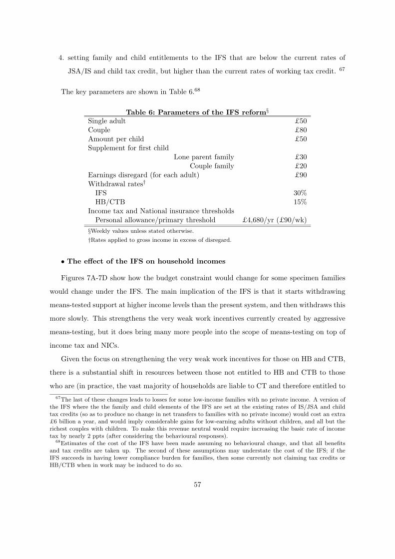
4. setting family and child entitlements to the IFS that are below the current rates of

JSA/IS and child tax credit, but higher than the current rates of working tax credit. 67

The key parameters are shown in Table 6.68

Table 6: Parameters of the IFS reform§

Single adult £50Couple £80Amount per child £50Supplement for first child

Lone parent family £30Couple family £20

Earnings disregard (for each adult) £90Withdrawal rates†

IFS 30%HB/CTB 15%

Income tax and National insurance thresholdsPersonal allowance/primary threshold £4,680/yr (£90/wk)

§Weekly values unless stated otherwise.

†Rates applied to gross income in excess of disregard.

• The effect of the IFS on household incomes

Figures 7A-7D show how the budget constraint would change for some specimen families

would change under the IFS. The main implication of the IFS is that it starts withdrawing

means-tested support at higher income levels than the present system, and then withdraws this

more slowly. This strengthens the very weak work incentives currently created by aggressive

means-testing, but it does bring many more people into the scope of means-testing on top of

income tax and NICs.

Given the focus on strengthening the very weak work incentives for those on HB and CTB,

there is a substantial shift in resources between those not entitled to HB and CTB to those

who are (in practice, the vast majority of households are liable to CT and therefore entitled to67The last of these changes leads to losses for some low-income families with no private income. A version of

the IFS where the the family and child elements of the IFS are set at the existing rates of IS/JSA and childtax credits (so as to produce no change in net transfers to families with no private income) would cost an extra£6 billion a year, and would imply considerable gains for low-earning adults without children, and all but therichest couples with children. To make this revenue neutral would require increasing the basic rate of incometax by nearly 2 ppts (after considering the behavioural responses).

68Estimates of the cost of the IFS have been made assuming no behavioural change, and that all benefitsand tax credits are taken up. The second of these assumptions may understate the cost of the IFS; if theIFS succeeds in having lower compliance burden for families, then some currently not claiming tax credits orHB/CTB when in work may be induced to do so.

57

CTB, but only renters are eligible for HB). Whether the IFS reform implies an unacceptable

distortion to the housing market - by increasing rent subsidies, and doing nothing for home-

owners - takes us outside the scope of optimal tax theory and into issues related to housing

policy in the UK, but addressing this (perceived or actual) distortion would require either

reducing the generosity of housing benefit, or extending it to home-owners so that it is tenure-

neutral (with an accompanying general rise in tax to pay for this). Similarly, it is beyond the

scope of this chapter to consider whether council tax itself should be reformed; if it were made

less regressive, then it might be possible to do without council tax benefit.

Table 7 shows the impact of the IFS on net incomes of working-age adults, by family type,

and by decile group of equivalised income of working-age adults before any consideration of

behavioural effects. The main impacts of the IFS reform on net incomes are as follows.

• The maximum entitlements to the IFS are a little higher than current tax credit entitle-

ments but lower than current IS/JSA rates (except for lone parents), and this leads to

losses for IS/JSA recipients with no other sources of income. However, the fact that the

IFS is made available without any hours rules means that some low-income individuals

(particularly single adults with no children aged 25 or over working under 30 hours a

week) currently entitled to neither IS/JSA nor tax credits gain substantially.

• Low-income families entitled to HB/CTB tend to gain because the equivalent support is

withdrawn more slowly under the IFS.

• Better-off families with children tend to lose as support currently provided through the

non-means-tested child benefit is now tapered away as part of the IFS.

• All taxpayers lose slightly as the income tax personal allowance and the NICs primary

threshold has been cut slightly.

• All taxpayers lose as the main rate of income tax is increased.

Across the whole population, the bottom half of the income distribution tend to be better

off, and the top half to be worse off, but the changes are not entirely progressive: the largest

gains are in the middle of the bottom half of the distribution, and the largest losses are in the

58

middle of the top half.69

Table 7: Distributional impact of IFS: percentage income gainDecile overall singles couples couples lonegroup population no children no children with children parents

1 4.6% 4.1% 11.8% 1.4% 3.7%2 4.3% 6.2% 6.7% 3.6% 2.4%3 4.8% 2.4% 5.4% 6.1% 4.1%4 4.0% 3.0% 3.8% 5.1% 2.7%5 0.9% 2.1% 0.9% 0.1% 1.2%6 -1.7% 1.3% -0.1% -4.6% 0.3%7 -2.4% 0.5% -0.4% -6.2% -0.2%8 -2.2% 1.4% -1.2% -5.4% -2.5%9 -1.6% 0.9% -1.2% -3.9% -3.2%10 -1.2% -0.4% -1.1% -2.1% -1.5%

Note: based on uprated data from the Family Resources Survey 2004/5 and the Institute for

Fiscal Studies’ tax and benefit micro-simulation model, TAXBEN.

Figures 8A to 8H show the impact of the IFS on (mean) PTRs and METRs by earnings

for the same four family types.70 In general, PTRs are lowered for all adults with low earn-

ings, reflecting the universal £90 earnings disregard, and the lower out-of-work safety net for

some. For some adults in families with children, the IFS increases PTRs on higher earnings,

reflecting that support currently provided through the non-means-tested child benefit would

be withdrawn as part of the IFS.

The impact on METRs is more complex. All family types see a fall in METRs on earnings

below £90, reflecting that the £90 earnings disregard in the IFS is much higher than in current

means-tested benefits. Above this, there are different patterns for the different family types.

Lone parents and primary earners in couples with children tend to see METRs fall slightly at

low earnings (that are above £90) but rise at higher earnings: this directly reflects that the

IFS taper is lower than the current tax credit taper, and that the IFS taper extends further up

the earnings distribution than the tax credit taper does currently. However, the other family69Another statistic summarising the impact on the income distribution is the impact on relative poverty rates.

Calibrating the poverty line so that 21% of children are in relative poverty (the rate in 2004/5, where povertyis defined as living in a household with less than 60% of median equivalised income), child poverty falls by 1.4ppts, or just under 200,000 children before allowing for behavioural responses (but allowing the IFS reform toshift the median).

70These Figures are based on estimates of the METR and PTR of each working adult in the 2004/5 FRSmade using TAXBEN. All Figures plot individual earnings on the horizontal axis.

59

types tend to see rises in METRs because more of these adults are affected by the withdrawal

of the IFS than are currently affected by a withdrawal of tax credits (for single adults without

children, this is predominantly because many more are entitled to the IFS as it has no hours

of work limits; for second earners in couples with children, it is predominantly because the

lower IFS withdrawal rate means that its withdrawal extends further up the (family) earnings

distribution).

The online appendix explains how simple estimates of the behavioural response to the IFS

affect the cost to the Exchequer, employment and total hours worked (or total earnings). These

show that, given reasonable assumptions on the size of behavioural responses, the impact of

the IFS reform on the Exchequer is small but negative. The IFS reform would be expected to

lead to more people participating in the labour market, but average earnings conditional on

participation falls, with the overall effect on total earnings being negative.71

Part of the reason for this negative behavioural response is that we have tried to reduce

the generosity of the system for those with no private income by relatively small amounts, and

we have made no cuts at all in the generosity of HB/CTB. If those programmes were made

less generous to those with no private income, then income tax rates could be lowered, and

the overall impact of the IFS would be to increase total earnings. However, with the rates

proposed here, the achievement of the IFS is that it manages to redistribute more income with

minimal impact on total earnings and total net tax revenue, by targeting net tax cuts where

incentives to work are currently at their weakest.

8.3 Conclusion71It is not possible to estimate the impact of the behavioural responses on relative poverty rates, because

the behavioural responses are modelled at an individual level. But it is possible to say something for singleadult families. For lone parents, using a calibrated poverty line so that 21% of children were in relative povertyin the base system, 41% of children in lone parents were in poverty. Before behavioural responses, this fallsto 40% (70% for children with a workless lone parent, 7% for children with a working lone parent, with 48%of children having a working lone parent). The estimated impact of behavioural responses is to increase thenumber of children with a working lone parent by 3.4 ppts, and to cut the poverty rate of children with workinglone parents to 5%. Together, this makes the poverty rate for all children in lone parent families equal to 38%.

60

This paper has provided an overview of the lessons that have been learned over the last 30

years in the economics literature for the optimal design of household tax and benefits, and

an application to the United Kingdom. We derived formulae for the optimal tax rates using

the simple Mirrlees model, and showed the result of simulations of the whole tax system

based on the UK earnings distribution and empirically-estimated labor supply elasticities. We

investigated the link between top incomes and top marginal income tax rates since the 1960s.

We discussed how the optimal tax system is affected by allowing for participation responses,

migration, and how families and children should be treated.

These insights from optimal tax theory were contrasted with the work incentives inherent

in the current UK tax and benefit system, and it is worth repeating our conclusions.

First, participation tax rates at low earnings are high: for most groups, they are close

to 100% for jobs of too few hours to grant individuals entitlement to the working tax credit,

and they remain high even with it. Secondly, the phasing-out of the working and child tax

credits, which operates on top of national insurance and income tax, generates METRs of

73.4% (including employer NICs) for a large number of low to moderate earners which is likely

to be above the optimum rate even with modest behavioral responses. Third, the main means-

tested programme to help with housing (housing benefit) has an extremely high withdrawal rate

(further increasing METRs), administrative difficulties and problems of mis-perception which

deter low-income working families from claiming it. Finally, while the system for administering

income tax and NICs in the UK is simple and efficient, the systems for administering child

and working tax credits, and for housing benefit and council tax benefit, are administratively

burdensome for claimants, relatively expensive for the government, and prone to large amounts

of fraud and error: all mean that neither are as well-targeted on the economic situation of

beneficiaries as they could be.

Given this, we suggest a set of changes to the existing tax and benefit structure that

could be made immediately based on the lessons from our analysis. Our package of “imme-

diate reforms” is costly, and involves increasing the level of earnings disregards in all of the

means-tested benefits to reduce PTRs on low earnings and introducing an additional earnings

disregard in tax credits for second earners to reduce PTRs for secondary earners, particularly

those with children. Work incentives can be further improved by reductions in the withdrawal

rate in child and working tax credits, and by targeting increases in the working tax credit on

61

groups other than lone parents.

We also provide a more radical and comprehensive plan for reforming the UK household

tax and benefit system that attempts to deal not only with these work incentive issues, but

also the administrative failings that we identify. Our plan replaces the piece-meal benefits

for low-income families (income support, working and child tax credits, housing benefit and

council tax benefit) into a single Integrated Family Support programme which provides stronger

and simpler incentives for work at the bottom, reduces compliance costs for families, and

is provided “as-you-earn” and administered in the same way as NICs through the PAYE

withholding system. We show how this can be done in a revenue-neutral fashion, including an

assessment of the behavioural responses. The key achievement of the IFS is that it manages

to redistribute income with minimal impact on total earnings and total net tax revenue, by

targeting net tax cuts which work with the grain, rather than against the grain, of individuals’

work incentives.

We have used the framework of optimal tax theory to guide our discussion throughout this

chapter. We argued that one attractive feature of this theory is that it makes explicit that

one cannot hope to say how best to design taxes and transfers without specifying what one

is trying to achieve overall. This, of course, may prove to be our ultimate downfall. Without

knowing the government’s preferences for redistribution or other objectives, we cannot hope

to predict whether our reform will appeal.

Appendix

This section provides a more formal discussion of the derivation of optimal income tax

rates. We will first show how to determine the optimal marginal tax rate for high earners, and

then how to derive optimal tax rates for tax payers more generally.

• Determining the top rate of income tax

Consider a reform that changes the top tax rate τ by a small amount dτ (with no change

in the tax schedule for incomes below the top bracket z). Here, let us denote by z the average

income reported by taxpayers in the top bracket and let us assume that there are N taxpayers

in the top bracket. As mentioned in the main text, this small tax reform has the following

effects on tax revenue:

62

1. There is a mechanical increase in tax revenue because taxpayers face a higher MTR on

incomes above z. Hence, the total mechanical effect is dM = N [z − z]dτ > 0. This

mechanical effect is the projected increase in tax revenue if there were no behavioral

response.

2. The increase in the tax rate triggers a behavioral response which reduces the average

reported income in the top bracket by dz = −e ·z ·dτ/(1−τ) on average (by definition of

the elasticity e - see Box 1 in Section 3) and hence produces a loss in tax revenue equal

to dB = −N · e · z · dτ · τ/(1− τ) < 0.

Rather than necessarily assuming that the marginal value of consumption for top taxpayers

is negligible relative to the average person in the economy, let us assume that the government

values at g, giving 1 additional £to the average top bracket taxpayer. If the government values

redistribution, g will be strictly less than one, and will be zero if the government has strong

redistributive tastes (the case considered in the main text). Hence, the small tax reform also

creates a social welfare cost equal to dW = −g ·N [z − z] dτ < 0.

Summing the mechanical and the behavioral tax revenue effect and the welfare effect, we

obtain the net effect of the reform from the government perspective:

dM + dB + dW = Ndτ(z − z) ·[1− g − e · z

z − z· τ

1− τ

]At the optimum, this expression must be zero. As before, let us denote by a the ratio z/(z− z),

which measures the thinness of the top of the income distribution. Note that a ≥ 1. The

optimum τ can then be expressed as:

τ∗ =1− g

1− g + a · e. (1)

Unsurprisingly, the optimal tax rate is decreasing in g (the value that the government sets

on the marginal consumption of high incomes), decreasing in the elasticity e of behavioral

responses, and decreasing in a, the parameter which measures the thinness of the top of the

income distribution. Note that this expression is identical to that presented in Box 2 when

g = 0. This important case gives an upper bound on the optimal top rate equal to 1/(1 +a · e)

. This corresponds to the tax rate maximizing tax revenue from top bracket taxpayers: the so-

called Laffer rate. Finally, we note that it is well known that top tails of income distributions

63

are closely approximated by Pareto distributions,72 in which case the parameter a does not

vary with z and is exactly equal to the Pareto parameter.73

• Determining the optimal marginal tax schedules

We can extend the above analysis to consider how the optimal tax rate varies more gen-

erally across the income distribution. Here, we let T (z) denote the (possibly non-linear) tax

schedule that the government imposes, where z denotes a given level of earnings. This tax

schedule incorporates both transfers (when T (z) is negative) and taxes (when T (z) is positive).

Let us denote by H(z) the cumulative distribution of individuals (fraction of taxpayers with

income less than z) and by h(z) the density distribution of taxpayers. The optimal tax system

is characterized by a lumpsum grant received by those with no earnings (equal to −T (0))

combined with a schedule of marginal tax rates T ′(z) which define how the lumpsum grant

should be reduced at earnings increase and how additional earnings should be taxed once the

lumpsum grant is fully tapered out. Again, the optimal marginal tax rate T ′(z) is set so as to

balance costs and benefits at the margin.

Suppose that the government increases the marginal tax rate T ′(z) by dτ in a small band

of income (z, z + dz). As above, this reform has three effects on government tax receipts and

welfare:

1. The reform increases taxes by dτdz for every taxpayer above the small band, and hence

collects extra taxes dM = (1−H(z))dτdz.

2. Those extra taxes generate a welfare cost to taxpayers. If we denote by G(z) the aver-

age social value for the government of distributing £1 uniformly among taxpayers with

income above z, the welfare cost is simply dW = dM ·G(z).74 If the government values

redistribution, G(z) will be decreasing in z. As we have assumed away income effects,

G(0) = 1.75, and we assumed above that G(z) goes to zero when z is large (i.e. in the top72A Pareto distribution has a density function of the form f(z) = C/z1+α where C and α are constant

parameters. α is called the Pareto parameter.73When z reaches the level of the very highest income earner, z = z and a is infinite and the optimal tax

rate is zero, which is the famous Sadka-Seade zero top result. However, this zero top result is a very misleadingresult for practical tax policy as the empirical a does not go to infinity except for the very highest incomeearner.

74This is a consequence of the envelope theorem as each individual maximizes utility.75Distributing 1 pound uniformly among all individuals does not generate behavioral responses and hence

has a cost of exactly 1 pound for the government.

64

tax bracket). The more redistributive the tastes of the government, the smaller G(z).

3. The marginal tax rate increase dτ in the small band reduces earnings by −e · z · dτ/(1−

T ′(z)) for taxpayers in the small band due to the substitution effect. There are h(z)dz

such taxpayers in the small band, and so this produces a loss in tax revenue equal to

dB = −e · z · [T ′(z)/(1− T ′(z))]dτ · h(z)dz.

At the optimum, dM + dW + dB = 0, which generates the following optimal tax rate

formula:76

T ′(z)1− T ′(z)

=1e· 1−H(z)

zh(z)· (1−G(z))

The optimal tax rate T ′(z) is decreasing with the elasticity e. It is also decreasing in G(z)

which measures the social marginal value of consumption for individuals with earnings above

z, and decreasing in the hazard ratio (1 −H(z))/(zh(z)) which measures the thinness of the

distribution.

• Optimal tax rates with participation responses

Here, an individual with skill z who decides to work will get z−T (z) in disposable income.

If the individual decides not to work, she will get −T (0) in disposable income. We assume

that individual utility is simply u = c−q where c is disposable income and q are costs of work.

Hence, the individual will work if the net return to work z − T (z) + T (0) exceeds her costs

of working which we denote by q. If we assume that costs of work q are distributed with a

(cumulated) distribution P (q|z) among individuals with skill z, the number of individuals of

skill z who work is simply P (z − T (z) + T (0)|z). We can define the elasticity of participation

with respect to the net return to work as:

η(z) =z − T (z) + T (0)

P· ∂P∂q

. (2)

To derive an optimal tax formula, let us consider a small increase in dT in T (z) but only

at skill level z. As there are only extensive responses, this reform affects only individuals with76This formula is not exactly accurate but very close for discussion and intuition purposes. In the exact

formula, h(z) should be replaced with the “virtual” density h∗(z), which is the density of earnings at z thatwould arise if the tax system were replaced by the linearized tax system at z. See Saez (2001) for completedetails.

65

skill z. As above, this reform has three effects on government tax receipts and welfare:

1. The reform increases taxes by dT for every taxpayer with skill z who works and hence

collects extra taxes dM = P (q|z)dT .

2. The extra taxes that are now collected generate a welfare cost to workers with skill z.

If we denote by g(z) the social value for the government of distributing 1 pound among

taxpayers with income z, the welfare cost is simply dW = dM · g(z) = P (q|z)g(z)dT .

If the government values redistribution, g(z) will be decreasing in z. The “no income

effect” assumption implies that the average g(z) across the full population is equal to

one.. The g(z) of this section and the G(z) of previous section are related by the formula

G(z)(1−H(z)) =∫∞z g(z)h(z)dz.

3. The tax increase dT at income level z induces some of the workers at z to drop out of

work. All those with fixed cost of work q between z−T (z)+T (0)−dT and z−T (z)+T (0)

drop out. There are dT∂P/∂q = dTηP/(z − T (z) + T (0)) such workers. The fiscal cost

of this behavioral response is dB = [(T (z)− T (0))/(z − T (z) + T (0))] · η · P (q|z)dT .77

To proceed, define the participation tax rate, a measure of the extent to which the tax and

benefit system weakens the reward from working t(z) = (T (z)− T (0))/z. As discussed above,

1− t(z) measures the increase in disposable income (relative to earnings) when an individual

decides to work. Using this definition, and noting that at the optimum we again must have

dM + dW + dB = 0, we generate the following optimal tax rate formula:

t(z)1− t(z)

=1η· (1− g(z)) (3)

This formula is a simple inverse elasticity tax rule for the average tax rate on work. The

average tax rate decreases with the elasticity η and also decreases with g(z), the social value

of marginal consumption for individuals earning z.

77Note that those dropping out of the labor force are indifferent (within dT ) between working and not workingand there is only an infinitesimal number of switchers. Hence the welfare effect on movers is second order relativeto the welfare effect on those who work and can be neglected. This is directly equivalent to the situation fromSection 2 where behavioral responses do not create a first order welfare effect.

66

References

Aaberge, R., Colombino, U. and Strøm, S. (1999) “Labor Supply in Italy: An Empirical

Analysis of Joint Household Decisions, with Taxes and Quantity Constraints”, Journal of

Applied Econometrics, 14, 403-422

Adam, S. (2005) “Measuring the marginal efficiency cost of redistribution in the UK”, IFS

Working Paper, W05/14

Adam, S. and Brewer, M. (2004), Supporting families: The financial costs and benefits of

children since 1975, The Policy Press: Bristol.

Adam, S., Brewer, M. and Shephard, A. (2006), The poverty trade-off: work incentives and

income redistribution in Britain, The Policy Press: Bristol.

Adam, S. and Browne, J. (2006), “A Survey of the UK Tax System”, Institute for Fiscal

Studies Briefing Note 9.

Adam, S., Brewer, M., Browne, J. and Phillips, D. (2007), “ Government financial support for

children across the United Kingdom: how does Northern Ireland compare?”, NICCY: Belfast.

Adam, S., Browne, J. and Heady, C. (2007), [title], chapter for Mirrlees review.

Adam, S., Emmerson C. and Kenley, A. (2007) “A survey of UK local government finance”,

IFS Briefing Note 74, http://www.ifs.org.uk/bns/bn74.pdf.

Adda, J., Dustmann, C., Meghir, C., and Robin, J-M. (2006) “Career Progression and Formal

versus On-the-Job Training”, IZA Discussion Papers 2260, Institute for the Study of Labor

(IZA)

Akerlof, George A. (1978). “The Economics of ‘Tagging’ as Applied to the Optimal Income

Tax, Welfare Programs, and Manpower Planning”, The American Economic Review, March,

68(1), pp. 8-19.

Alesina, A. and Andrea, I. (2007). “Gender based taxation.” Harvard University Working

Paper, April.

Anderberg, D., Kondylis, F. and Walker, I. (2007), “Partnership Penalities and Bonuses Cre-

ated by Two Major UK benefits”, forthcoming CESIfo Economic Studies [check].

Arrufat, J. and Zabalza, A. (1986), “Female Labor Supply with Taxation, Random Preferences,

67

and Optimization Errors”, Econometrica, 54(1), 47-64.

Atkinson, Anthony 2007. “Top Incomes in the United Kingdom over the Twentieth Cen-

tury.” in Anthony Atkinson and Thomas Piketty, eds., Top Incomes from a Historical and

International Perspective. Oxford: Oxford University Press.

Atkinson, A. and Leigh, A. (2004), “Understanding the Distribution of Top Incomes in Anglo-

Saxon Countries over the Twentieth Century”, Department of Economics, Australian National

University.

Baughman, R. and Dickert-Conlin, S. (2007) “The Earned Income Tax Credit and Fertility”,

Journal of Population Economics, forthcoming.

Bell, K., Brewer, M. and Phillips, D. (2007), “Lone Parents and Mini Jobs”, York: YPS:

Blow, Laura and Ian Preston, 2002. “Deadweight Loss and Taxation of Earned Income:

Evidence from Tax Records of the UK Self-Employed”, IFS Working Paper No. 02/15.

Blundell, Richard, Chiappori, Pierre-Andre, and Costas Meghir. “Collective Labor Supply

with Children”, Journal of Political Economy, 113(6), 1277-1306, 2005.

Blundell, R. and MaCurdy, T., 1999. Labour Supply: A Review of Alternative Approaches. In:

Ashenfelter, O., Card, D. (Eds.), Handbook of labour Economics, Volume 3A, North-Holland,

Amsterdam.

Blundell, R. and Shephard, A., 2008. “Employment, Hours of Work and the Optimal Design

of Earned Income Tax Credits”, IFS Working Paper W08/01

Boskin, Michael and Eytan Sheshinski (1983). “Optimal Tax Treatment of the Family: Mar-

ried Couples.” Journal of Public Economics 20, 281-297.

Bowler, T. (2007), ”Taxation of the Family”, TLRC Discussion Paper 6, http://www.ifs.org.uk/comms/dp6.pdf,

London: IFS

Brewer, M., (2006), ”Tax Credits Fixed or Beyond Repair?” in R. Chote, C. Emmerson, R.

Harrison and D. Miles (eds), The IFS Green Budget 2006, London: IFS.

Brewer, Mike (2007), ”Supporting Couples with Children Through the Tax System” in R.

Chote, C. Emmerson, A. Leicester and D. Miles (eds) The IFS Green Budget 2007, London:

IFS.

68

Brewer, Mike, Browne, J., Emmerson, C., Goodman, A., Muriel, A. and Tetlow, G. (2007),

Pensioner Poverty over the next decade: what role for tax and benefit reform?, Commentary

103, London: IFS.

Brewer, Mike, Duncan, A., Shephard, A., Suarez, M.J., 2006 ”Did working families’ tax credit

work? The impact of in-work support on labour supply in Great Britain”. Labour Economics

13, 699-720.

Brewer, Mike and Shaw, Jonathan (2006), “How Many Lone Parents are Receiving Tax Cred-

its?”, Institute for Fiscal Studies Briefing Note 70.

Brewer, Mike , Ratcliffe, A. and Smith, S. (2007), “Does welfare reform affect fertility? Evi-

dence from the UK”, CMPO Working Paper 07/177.

Brewer et al (2008) P47

Brewer et al (2001) P40

Brewer et al (forthcoming) P32

Chiappori, Pierre-Andre. “Rational Household labour Supply.” Econometrica, 56(1):63–90,

1988.

Chiappori, Pierre-Andre. “Collective labour Supply and Welfare”. Journal of Political Econ-

omy, 100(3):437–467, 1992.

Cm 7130, 2006-7, ”In Work, Better Off”. London: TSO.

Cm 7290 (2006-7), ”Ready for Work: Full Employment in our generation”, London: TSO.

Community Links, Low Incomes Tax Reform Group and Child Poverty Action Group (2007),

”Interact: benefits, tax credits and moving into work”, London: Community Links, Low In-

comes Tax Reform Group and Child Poverty Action Group.

Cooke, G. and Lawton, K. (2008) “Working out of Poverty: A study of the low paid and

working poor”, http://www.ippr.org/publicationsandreports/publication.asp?id=581.

DWP (2007a), ”Fraud and Error in the Benefit System April 2005 to March 2006”, http://www.dwp.gov.uk/asd/asd2/fem/fem apr05 mar06.pdf.

Devereux, P. (2004) “Changes in Relative Wages and Family Labor Supply”, Journal of Human

Resources, Vol. 39, No. 3. (Summer, 2004), pp. 696-722.

69

Di Tommaso, M.L., Dex, S. and Rowthorn, R.E. (1999) “Women’s Labour Supply Decisions

in the Light of Possible Fiscal Reforms,” Research Paper WP36/99, Judge Institute of Man-

agement, University of Cambridge.

Diamond, Peter (1980) “Income Taxation with Fixed Hours of Work,” Journal of Public Eco-

nomics, 13, 101-110.

Diamond, Peter (1998). “Optimal Income Taxation: An Example with a U-Shaped Pattern

of Optimal Marginal Tax Rates.” American Economic Review 88, 83-95.

Dilnot, A., Kay, J. and Morris, N. (1984), The Reform of Social Security, Oxford: Clarendon

Press.

Dilnot, Andrew, and Michael Kell (1988). “Top-Rate Tax Cuts and Incentives: Some Empirical

Evidence.” Fiscal Studies 9, 70-92.

Draper, D. (2007). “Families Compared 2006/7”, CARE Research Paper, http://www.care.org.uk/Publisher/File.aspx?ID=13022.

Eissa, N. and Hoynes, H. (2000) “Explaining the Fall and Rise in the Tax Cost of Marriage:

The Effect of Tax Laws and Demographic Trends, 1984-1997,” National Tax Journal, Volume

53, Number 3, Part 2, pp. 683-711.

Eissa, N. and Hoynes, H. (2004) “Taxes and the Labor Market Participation of Married Cou-

ples: The Earned Income Tax Credit”, Journal of Public Economics, Volume 88, Number 9-10,

pp. 1931-1958.

Gentry, William R. and Glenn Hubbard (2004) “Success Taxes, Entrepreneurial Entry, and

Innovation”, NBER Working Paper No. 10551.

Griffith, R. and Klemm, A. (2004) What has been the tax competition experience of the last

20 years? Tax Notes International, Vol. 34, No. 13, pp. 1299-1316.

Gruber, Jon, and Saez, Emmanuel, 2002. The Elasticity of Taxable Income: Evidence and

Implications, Journal of Public Economics, 84, 1-32.

Guesnerie, Roger and Roberts, Kevin, 1984. “Effective policy tools and quantity controls.”

Econometrica 52, 59-86.

Harker, L. (2006) Delivering on Child Poverty: what would it take?, A report for the Depart-

ment for Work and Pensions, Cm 6951, November 2006

70

Heim, B.T. and Meyer, B., 2004. ”Work costs and nonconvex preferences in the estimation of

labour supply models”. Journal of Public Economics 88 (11), 2323– 2338.

Hills et al (2006) P48

HMRC (2007), ”Child Tax Credit and Working Tax Credit Take-up rates 2004-05”, http://www.hmrc.gov.uk/stats/personal-tax-credits/takeup-rates2004-05.pdf.

HMRC (2007b), ”Child and Working Tax Credits: Error and Fraud statistics, 2004-05”,

http://www.hmrc.gov.uk/stats/personal-tax-credits/cwtc-error0405.pdf.

HMRC (2007c), ”Number of individual income taxpayers”, http://www.hmrc.gov.uk/stats/income tax/table2-

1.pdf.

Hotz, V.J. and Scholz, J.K., 2003. ”The earned income tax credit”. In: Moffitt, R. (Ed.),

Means-Tested Transfer programmes in the U.S. University of Chicago Press.

HC 42-I (2007-08) ”The Best Start in Life? Alleviating deprivation, improving social mobility

and eradicating child poverty”, London: TSO.

HC 609 (2006-07) ”Helping People from workless households into work”, London: TSO

Hoynes, H. (1997) “Work, welfare and family structure” in Auerbach, A. (ed) Fiscal policy:

Lessons from economic research.

Hoynes, H. (2007) [Title] Chapter for Mirrlees Review

Immervoll, Herwig, Henrik Kleven, Claus Kreiner, and Emmanuel Saez, 2007. “Welfare Re-

form in European Countries: Microsimulation Analysis”, Economic Journal, [vol number],

1-44.

Kanbur, R., Keen, M. Tuomala, M. (1994),“Optimal Non-linear Income Taxation for the

Alleviation of Income-Poverty”, European Economic Review, 38, 1613-32.

Kirby, J. (2005), The Price of Parenthood, London: Centre for Policy Studies.

Kleven, Henrik, Claus Kreiner, and Emmanuel Saez, 2006. “The Optimal Taxation of Cou-

ples”, NBER Working Paper No. 12685.

Kluve, Jochen, Card, D., Fertig, M., Gora, M., Jacobi, L., Jensen, P., Leetmaa, R., Nima,

L., Patacchini, E., Schaffner, S., Schmidt, C.M., van der Klaauw, B., Weber, A. 2007. Active

Labor Market Policy in Europe: Performance and Perspectives, Springer: Berlin et al.

71

Laroque, G. and Salanie, B. (2005), “Fertility and Financial Incentives in France”, CESIfo

Economic Studies, 50(3), 423-450.

Lundberg, Shelly J., Robert A. Pollak, and Terence J. Wales (1997). “Do Husbands and

Wives Pool Their Resources: Evidence from the United Kingdom Child Tax Credit.” Journal

of Human Resources, 32(3), 463–480.

Meghir, C. and Phillips, D., chapter for Mirrlees review.

Milligan, K. (2005), “Subsidizing the Stork: New Evidence on Tax Incentives and Fertility”,

Review of Economics and Statistics, 87(3), 539-555.

Mirrlees, J., 1971. An Exploration in the Theory of Optimal Income Taxation. Review of

Economic Studies, 38, 175-208.

Mirrlees, James A. (1982) “Migration and Optimal Income Taxes.”, Journal of Public Eco-

nomics, 18(3), 319-41.

Moffitt, R. (2006) “Welfare Work Requirements with Paternalistic Government Preferences”,

Economic Journal, 116 (515) , F441–F458

O’Dea, C., Phillips, D. and Vink, A. (2007), “A Survey of the UK Benefit System”, Institute

for Fiscal Studies Briefing Note 13.

Pencavel (1986) “Labor Supply of Men: A Survey” in Orley Ashenfelter and Richard Layard,

eds., Handbook of Labor Economics Volume 1, Amsterdam: North-Holland, 1986, 3-102.

Piketty, Thomas and Emmanuel Saez (2007). “How Progressive is the U.S. Federal Tax Sys-

tem? A Historical and International Perspective.” Journal of Economic Perspectives 21(1),

3-24.

Saez, Emmanuel (2001). “Using Elasticities to Derive Optimal Income Tax Rates.” Review of

Economic Studies 68, 205-229.

Saez, Emmanuel, (2002a). “Optimal Income Transfer programmes: Intensive Versus Extensive

labour Supply Responses.” Quarterly Journal of Economics, 117.

Saez, Emmanuel, (2002b). “Do Taxpayers Bunch at Kink Points?” Working Paper [more

detail].

Saez, Emmanuel (2004). “Reported Incomes and Marginal Tax Rates, 1960-2000: Evidence

72

and Policy Implications.” in Ed. James Poterba, Tax Policy and the Economy, 18.

Simula, L. and Trannoy, A. (2006). “Optimal Non-Linear Income Tax when Agents Vote with

their Feet”, Finanzarchiv, 62 (3), 393-415

Shaw, J, Slemrod, J. and Whiting, 2007, chapter for Mirrlees review

Social Justice Policy Group (2007), ”Breakthrough Britain”, London: Social Justice Policy

Group.

Turley, C. and Thomas, A (2006), Housing Benefit and Council Tax Benefit as in-work benefits;

claimants’ and advisors’ knowledge, attitudes and experiences, DWP Research Report 383,

Leeds: CDS.

Whiteford, P., Mendelson, M. and Millar, J. (2003), Timing it right? Tax credits and how to

respond to income changes. York: JRF.

73

Notes:

Assumes a lone parent with two children, paying £80 per week in rent,no childcare costs, average Band C council tax, and with a wage of £5.52 per hour.Incomes are calculated under the April 2008 tax and benefit systemwith announced changes to the higher-rate threshold and UEL.

Figure 1B: Participation and marginal tax rates

0%

20%

40%

60%

80%

100%

120%

0 10000 20000 30000 40000 50000 60000 70000Cost to employer, £/year

Part

icip

atio

n ta

x ra

te

PTRMTR

Figure 1A: Example budget constraint, lone parent

0

10000

20000

30000

40000

50000

60000

0 10000 20000 30000 40000 50000 60000 70000

Cost to employer, £/year

Net

Inco

me,

£/y

ear

Note: Income shares from Atkinson but 1962-1989 are adjusted up by 5% (factor 1.05) so that continuity from 1989 to 1990 when filing shifts from couples to individual

Figure 2A: Top 1% Income Share and Marginal Tax Rate

0%

10%

20%

30%

40%

50%

60%

70%

80%

1962

1966

1970

1974

1978

1982

1986

1990

1994

1998

2002

Mar

gina

l Tax

Rat

e

0%

2%

4%

6%

8%

10%

12%

14%

16%

Inco

me

Shar

e

Top 1% MTR excluding consumption taxes

Top 1% MTR including consumption taxes

Top 1% income share

Figure 2B: Top 5-1% Income Share and Marginal Tax Rate

0%

10%

20%

30%

40%

50%

60%

70%

80%

1962

1966

1970

1974

1978

1982

1986

1990

1994

1998

2002

Mar

gina

l Tax

Rat

e

0%

2%

4%

6%

8%

10%

12%

14%

16%In

com

e Sh

are

Top 5-1% MTR excluding consumptiontaxesTop 5-1% MTR including consumptiontaxesTop 5-1% income share

Figure 3: Hazard rate in the UK, 2003/04

0.0

0.1

0.2

0.3

0.4

0.5

0.6

0.7

0.8

0.9

1.0£0

£50,

000

£100

,000

£150

,000

£200

,000

£250

,000

£300

,000

£350

,000

£400

,000

Annual Gross Earnings

Haz

ard

Rat

e

Figure 4A: Optimal tax sensitivity, labor elasticity

0%

10%

20%

30%

40%

50%

60%

70%

80%

90%

100%£0

£50,

000

£100

,000

£150

,000

£200

,000

£250

,000

£300

,000

£350

,000

£400

,000

£450

,000

£500

,000

Annual Gross Earnings

Mar

gina

l Tax

Rat

e

elasticity=0.50

elasticity=0.25

Figure 4B: Optimal tax sensitivity, redistribution preference

0%

10%

20%

30%

40%

50%

60%

70%

80%

90%

100%

£0

£50,

000

£100

,000

£150

,000

£200

,000

£250

,000

£300

,000

£350

,000

£400

,000

£450

,000

£500

,000

Annual Gross Earnings

Mar

gina

l Tax

Rat

e

Rawlsian

gamma=1

Figure 5A-1: Budget constraint, lone parent

0

10000

20000

30000

40000

50000

60000

0 10000 20000 30000 40000 50000 60000 70000

Cost to employer, £/year

Net

Inco

me,

£/y

ear

Budget constraint

Budget constraint (inc. housing benefit)

Figure 5B-1: Participation tax rate, lone parent

0%

20%

40%

60%

80%

100%

120%

0 10000 20000 30000 40000 50000 60000 70000Cost to employer, £/year

Part

icip

atio

n ta

x ra

te

PTRPTR (inc. housing benefit)Empirical PTR

Notes:

Assumes a lone parent with two children, paying £80 per week in rent,no childcare costs, average Band C council tax, and with a wage of £5.52 per hour.Incomes are calculated under the April 2008 tax and benefit systemwith announced changes to the higher-rate threshold and UEL.

Figure 5C-1: Marginal tax rates, lone parent

0%

20%

40%

60%

80%

100%

120%

0 10000 20000 30000 40000 50000 60000 70000

Cost to employer, £/year

Mar

gina

l tax

rate

s

MTRMTR (inc.housing benefit)Empirical MTR

Figure 5A-2: Budget constraint, single no children

0

10000

20000

30000

40000

50000

60000

0 10000 20000 30000 40000 50000 60000 70000

Cost to employer, £/year

Net

Inco

me,

£/y

ear

Budget constraint

Budget constraint (inc. housing benefit)

Figure 5B-2: Participation tax rate, single no children

0%

20%

40%

60%

80%

100%

120%

0 10000 20000 30000 40000 50000 60000 70000

Cost to employer, £/year

Part

icip

atio

n ta

x ra

te

PTRPTR (inc. housing benefit)Empirical PTR

Notes:

Assumes a single adult without children, paying £80 per week in rent,average Band C council tax and with a wage of £5.52 per hour.Incomes are calculated under the April 2008 tax and benefit systemwith announced changes to the higher-rate threshold and UEL.

Figure 5C-2: Marginal tax rates, single no children

0%

20%

40%

60%

80%

100%

120%

0 10000 20000 30000 40000 50000 60000 70000

Cost to employer, £/year

Mar

gina

l tax

rate

sMTRMTR (inc.housing benefit)Empirical MTR

Figure 6A: PTR, Couples with and without children

-0.1

0.0

0.1

0.2

0.3

0.4

0.5

0.6

0.7

0.8

0.9

1.0

0 10000 20000 30000 40000 50000 60000 70000

Cost to employer, £/year

Part

icip

atio

n ta

x ra

te

without children: partner doesn't workwithout children: partner workswith children: partner doesn't workwith children: partner works

Figure 6B: MTR, Couples with and without children

-0.1

0.0

0.1

0.2

0.3

0.4

0.5

0.6

0.7

0.8

0.9

1.0

0 10000 20000 30000 40000 50000 60000 70000

Cost to employer, £/year

Part

icip

atio

n ta

x ra

te

without children: partner doesn't workwithout children: partner workswith children: partner doesn't workwith children: partner works

Figure 7A: IFS Reform, budget constraint, lone parents

0

10000

20000

30000

40000

50000

60000

0 10000 20000 30000 40000 50000 60000

Cost to employer, £/year

Net

Inco

me,

£/y

ear

Base Budget constraint (inc. housing benefit)

IFS Budget constraint (inc. housing benefit)

Figure 7B: IFS Reform, budget constraint, one earner couple with children

0

10000

20000

30000

40000

50000

60000

0 10000 20000 30000 40000 50000 60000

Cost to employer, £/year

Net

Inco

me,

£/y

ear

Base Budget constraint (no housing benefit)

IFS Budget constraint (no housing benefit)

Figure 7C: IFS Reform, budget constraint, single no children

0

10000

20000

30000

40000

50000

60000

0 10000 20000 30000 40000 50000 60000

Cost to employer, £/year

Net

Inco

me,

£/y

ear

Base Budget constraint (inc. housing benefit)

IFS Budget constraint (inc. housing benefit)

Figure 7D: IFS Reform, budget constraint, one earner couple without children

0

10000

20000

30000

40000

50000

60000

0 10000 20000 30000 40000 50000 60000

Cost to employer, £/year

Net

Inco

me,

£/y

ear

Base Budget constraint (no housing benefit)

IFS Budget constraint (no housing benefit)

Figure 8A: PTR - Singles no children, impact of reform

-10%

0%

10%

20%

30%

40%

50%

60%

70%

80%

90%

100%

0 10000 20000 30000 40000 50000 60000 70000

Cost to employer, £/year

Part

icip

atio

n ta

x ra

te

basereform

Figure 8B: MTR - Singles no children, impact of reform

-10%

0%

10%

20%

30%

40%

50%

60%

70%

80%

90%

100%

0 10000 20000 30000 40000 50000 60000 70000

Cost to employer, £/year

Mar

gina

l tax

rate

basereform

Figure 8C: PTR - Lone parents, impact of reform

-10%

0%

10%

20%

30%

40%

50%

60%

70%

80%

90%

100%

0 10000 20000 30000 40000 50000 60000 70000

Cost to employer, £/year

Part

icip

atio

n ta

x ra

te

basereform

Figure 8D: MTR - lone parents, impact of reform

-10%

0%

10%

20%

30%

40%

50%

60%

70%

80%

90%

100%

0 10000 20000 30000 40000 50000 60000 70000

Cost to employer, £/year

Mar

gina

l tax

rate

basereform

Figure 8E: PTR - Couples no children, impact of reform

-10%

0%

10%

20%

30%

40%

50%

60%

70%

80%

90%

100%

0 10000 20000 30000 40000 50000 60000 70000

Cost to employer, £/year

Part

icip

atio

n ta

x ra

te

base: partner doesn't work

base: partner works

reform: partner doesn't work

reform: partner works

Figure 8F: MTR - Couples no children, impact of reform

-10%

0%

10%

20%

30%

40%

50%

60%

70%

80%

90%

100%

0 10000 20000 30000 40000 50000 60000 70000

Cost to employer, £/year

Part

icip

atio

n ta

x ra

te

base: partner doesn't work

base: partner works

reform: partner doesn't work

reform: partner works

Figure 8G: PTR - Couples with children, impact of reform

-10%

0%

10%

20%

30%

40%

50%

60%

70%

80%

90%

100%

0 10000 20000 30000 40000 50000 60000 70000

Cost to employer, £/year

Part

icip

atio

n ta

x ra

te

base: partner doesn't work

base: partner works

reform: partner doesn't work

reform: partner works

Figure 8H: MTR - Couples with children, impact of reform

-10%

0%

10%

20%

30%

40%

50%

60%

70%

80%

90%

100%

0 10000 20000 30000 40000 50000 60000 70000

Cost to employer, £/year

Part

icip

atio

n ta

x ra

te

base: partner doesn't work

base: partner works

reform: partner doesn't work

reform: partner works