measure projection analysis
TRANSCRIPT
Measure Projection Analysisor: how I learned to stop clustering
and love the grid.
Nima Bigdely-Shamlo, Tim Mullen, Ozgur Yigit BalkanSwartz Center for Computational Neuroscience
INC, UCSD, 2010
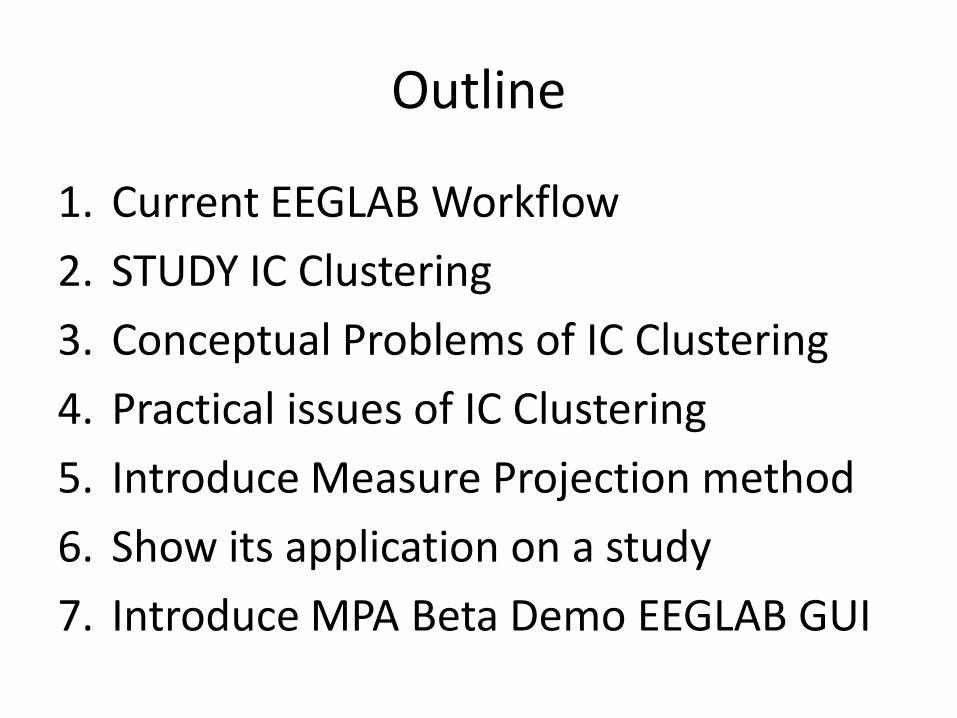
Outline
1. Current EEGLAB Workflow2. STUDY IC Clustering3. Conceptual Problems of IC Clustering4. Practical issues of IC Clustering5. Introduce Measure Projection method6. Show its application on a study7. Introduce MPA Beta Demo EEGLAB GUI

Current EEGLAB Workflow
Collect EEG Pre-Process (filter…)
Remove artifacts Run ICA Look at ICs
(maybe)
Single EEG Session Analysis
Select dipolar ICs from all sessions
Pre-compute EEG measures
(ERP, ERSP, ITC…)
Select clustering
parameters
Look at clusters
Until expectedresults are produced
Study Analysis
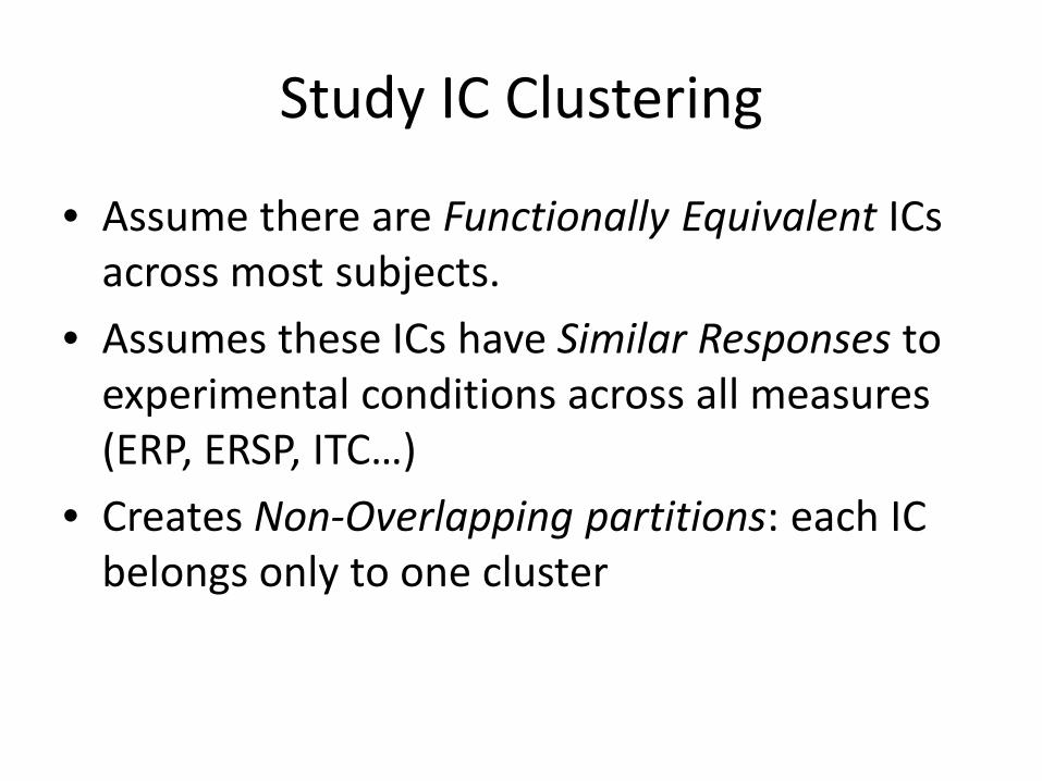
Study IC Clustering
• Assume there are Functionally Equivalent ICs across most subjects.
• Assumes these ICs have Similar Responses to experimental conditions across all measures (ERP, ERSP, ITC…)
• Creates Non-Overlapping partitions: each IC belongs only to one cluster
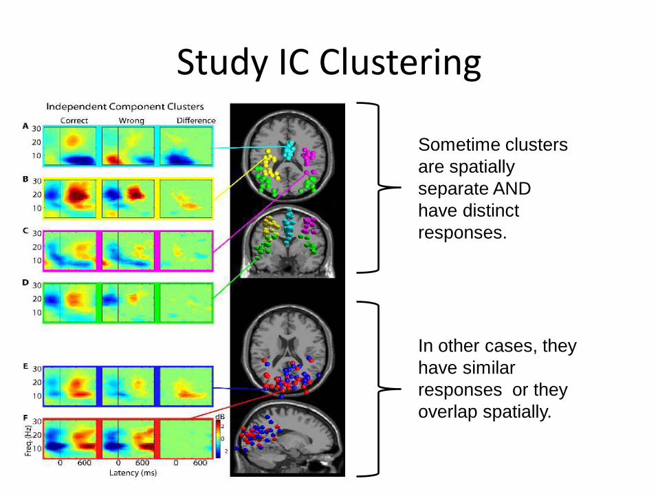
Study IC Clustering
Sometime clusters are spatially separate AND have distinct responses.
In other cases, they have similar responses or they overlap spatially.
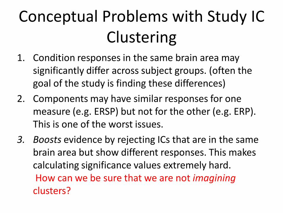
Conceptual Problems with Study IC Clustering
1. Condition responses in the same brain area may significantly differ across subject groups. (often the goal of the study is finding these differences)
2. Components may have similar responses for one measure (e.g. ERSP) but not for the other (e.g. ERP). This is one of the worst issues.
3. Boosts evidence by rejecting ICs that are in the same brain area but show different responses. This makes calculating significance values extremely hard.How can we be sure that we are not imaginingclusters?

ERP and ERSP have different similarity structures
Correlation between correlations = 0.21
EEGLAB sample (N400) study with 5 subjects (151 ICs) ADHD study with 132 subjects (3477 ICs)
rho= 1 rho= 1
Correlation between correlations = 0.11
This shows that ERSP and ERP generally have quite different similarity structures and it is probably not a good idea to combine them for clustering.
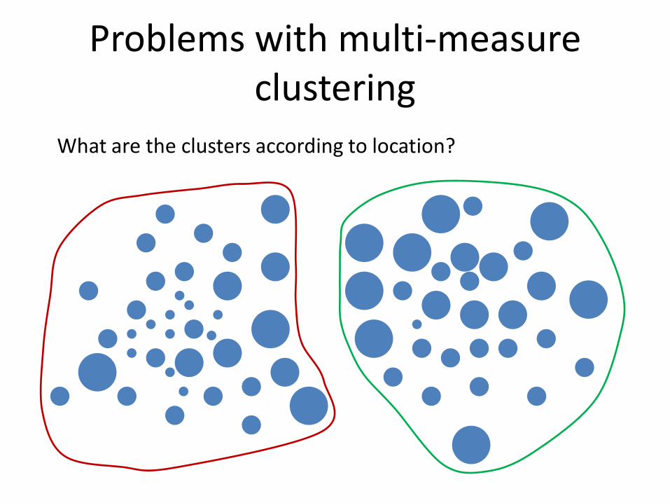
Problems with multi-measure clustering
What are the clusters according to location?
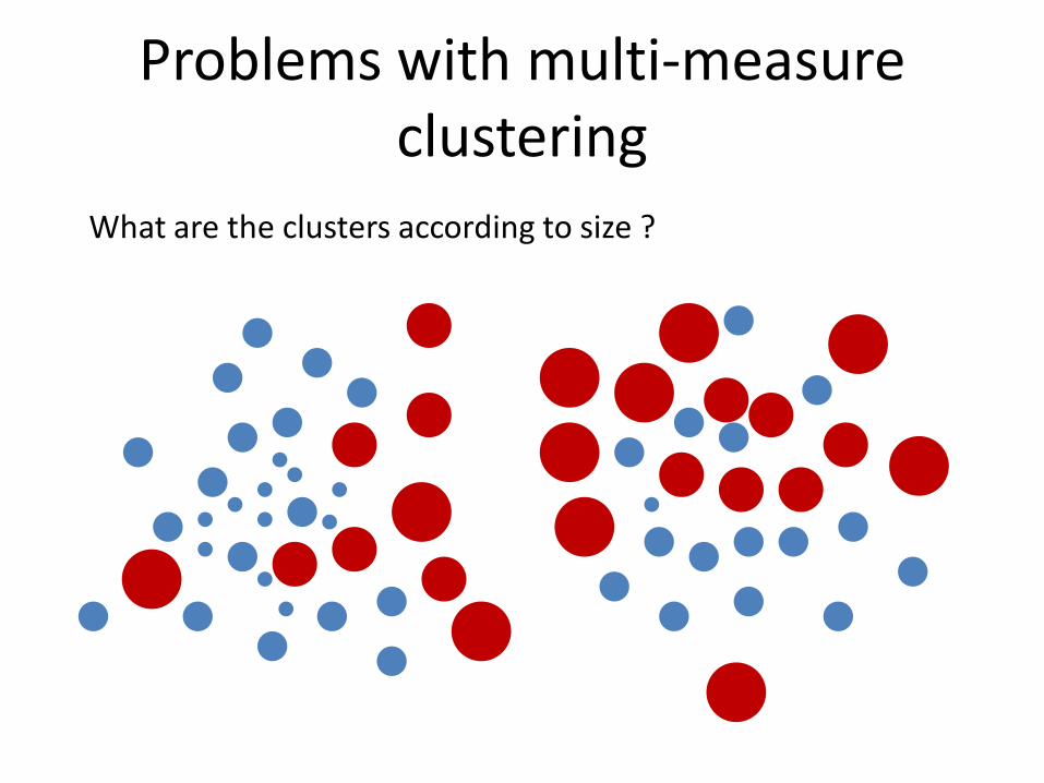
Problems with multi-measure clustering
What are the clusters according to size ?
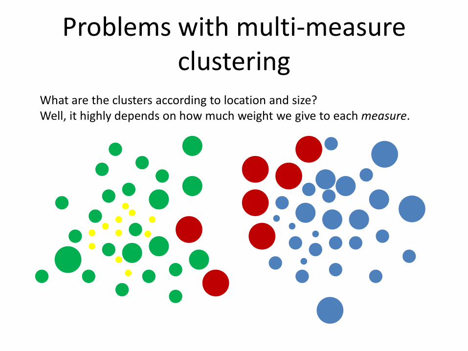
Problems with multi-measure clustering
What are the clusters according to location and size? Well, it highly depends on how much weight we give to each measure.
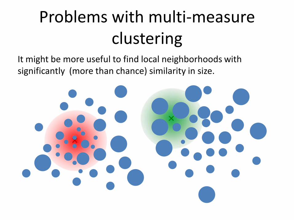
Problems with multi-measure clustering
It might be more useful to find local neighborhoods with significantly (more than chance) similarity in size.

Practical problems with current methods of Study IC Clustering
EEGLAB original clustering has ~12 parameters
Large parameter space problem: many different clustering solutions can be produced by changing parameters and measure subsets. Which one should we choose?
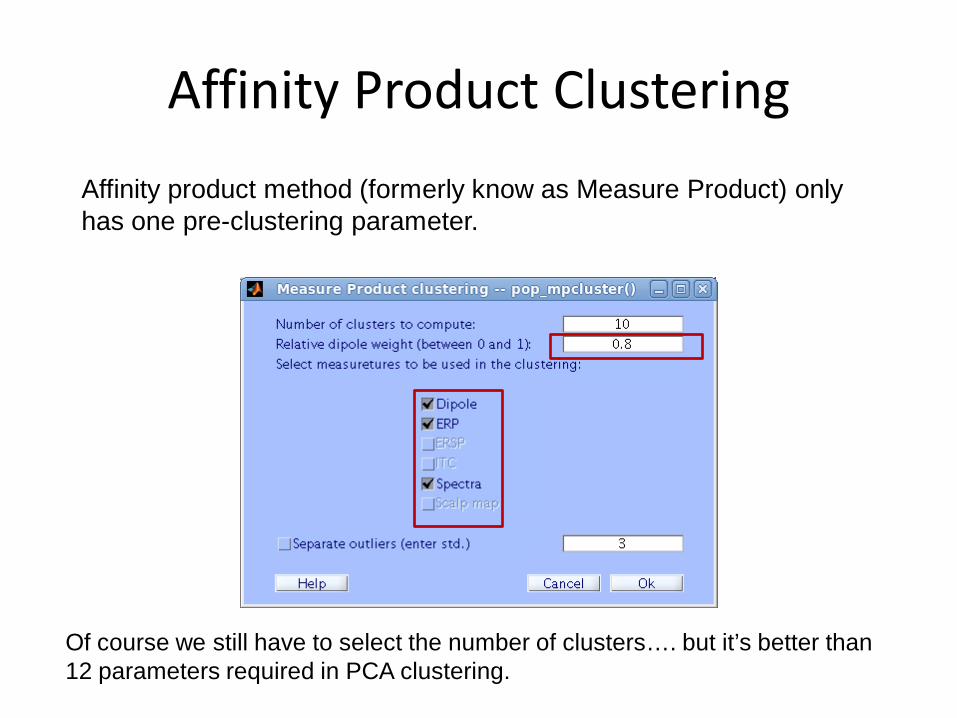
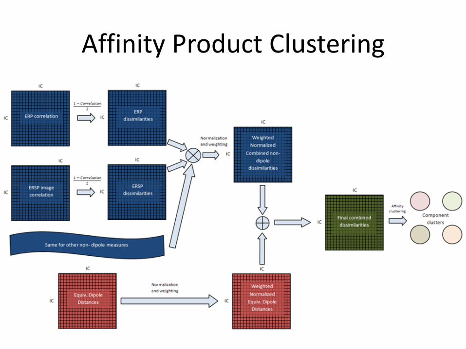
Affinity Product Clustering
Of course we still have to select the number of clusters…. but it’s better than 12 parameters required in PCA clustering.
Affinity product method (formerly know as Measure Product) only has one pre-clustering parameter.
Affinity Product Clustering

Practical problems with current methods of Study IC Clustering
• We still have to select the number of clusters.
• With both these clustering methods, we basically mix (either add or multiply) distances for a subset of EEG measures (ERP, ERSP, ITC, Spectrum, Dipole location) together. This makes clustering parameters less meaningful.

Study IC Clustering
IC Clusters are not necessarily incorrect, or imaginary, but it is quite hard to provide a good argument against such objections.

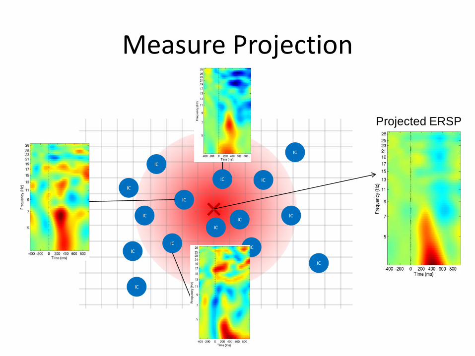
Measure Projection
• Instead of clustering, we assign to each location in the brain a unique EEG response.
• The response at each location is calculated as the weighted sum of IC responses in its neighborhood.
• Weights are assigned by passing the distance between the location and IC dipole through a Gaussian function.
• The std. of this function represent expected error in dipole localization and inter-subject variability.

Measure ProjectionGaussian weights (12 mm std.)
max
min

Measure Projection
• Each EEG measure (ERP, ERSP..) is projected separately.
• Only has one (1) parameter: std. of Gaussian (which has a biological meaning).
• Bootstrap (permutation) statistics can be easily and quickly performed for each point in the brain.
• A regular grid is placed in the brain to investigate every area (with ~10 mm or less spacing).
Measure Projection
IC
IC
IC
IC
IC
IC
ICIC
IC
IC
ICIC
IC
IC
IC
IC
Projected ERSP
Measure Projection
• Not all projected values are significant.• Some are weighted means of ICs with very dissimilar
responses.• Only projected values in neighborhoods with
convergent responses are significant.• Convergence can be expressed as the mean of
pairwise similarities in a spatial neighborhood.• The significance of convergence at each location can
be calculated with bootstrapping (permutation).
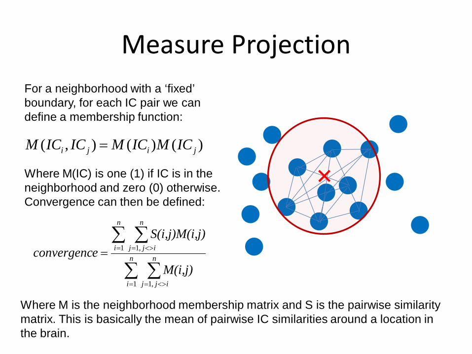
Measure ProjectionFor a neighborhood with a ‘fixed’ boundary, for each IC pair we can define a membership function:
Where M(IC) is one (1) if IC is in the neighborhood and zero (0) otherwise.Convergence can then be defined:
∑ ∑
∑ ∑
= <>=
= <>== n
i
n
ijj
n
i
n
ijj
M(i,j)
j)S(i,j)M(i,econvergenc
1 ,1
1 ,1
Where M is the neighborhood membership matrix and S is the pairwise similarity matrix. This is basically the mean of pairwise IC similarities around a location in the brain.
)()(),( jiji ICMICMICICM =
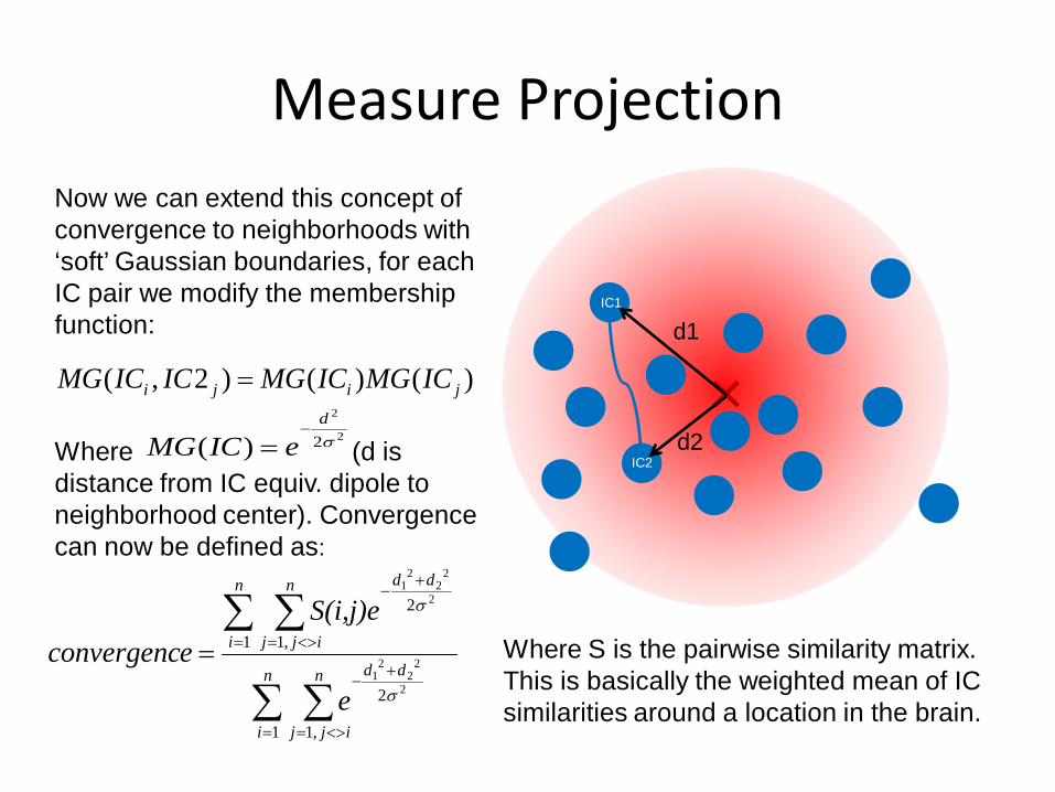
Measure ProjectionNow we can extend this concept of convergence to neighborhoods with ‘soft’ Gaussian boundaries, for each IC pair we modify the membership function:
Where (d is distance from IC equiv. dipole to neighborhood center). Convergence can now be defined as:
∑ ∑
∑ ∑
= <>=
+−
= <>=
+−
=n
i
n
ijj
dd
n
i
n
ijj
dd
e
S(i,j)eeconvergenc
1 ,1
2
1 ,1
2
2
22
21
2
22
21
σ
σ
Where S is the pairwise similarity matrix. This is basically the weighted mean of IC similarities around a location in the brain.
2
2
2)( σd
eICMG−
=
d1
d2
IC1
IC2
)()()2,( jiji ICMGICMGICICMG =
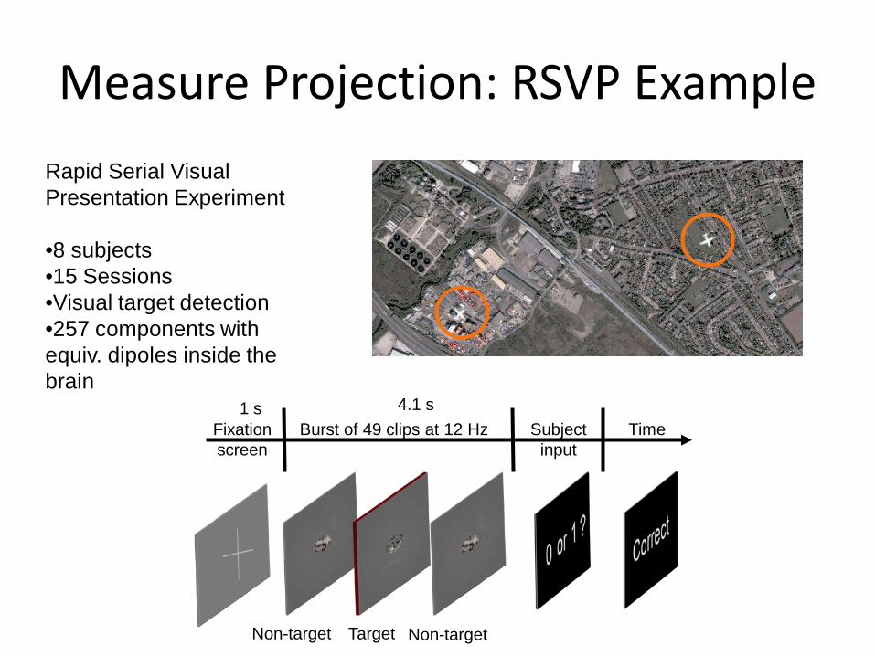
Measure Projection: RSVP Example
TimeSubject input
1 s 4.1 sBurst of 49 clips at 12 HzFixation
screen
Non-targetTargetNon-target
Rapid Serial Visual Presentation Experiment
•8 subjects•15 Sessions•Visual target detection•257 components with equiv. dipoles inside the brain

Measure Projection: RSVP Example
Mean weighted correlation in neighborhood
Areas in which convergence is significant (p<0.01).
Gaussian std. = 12 mm
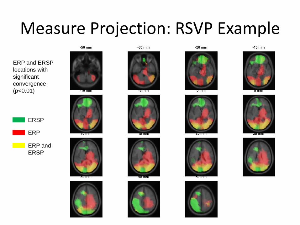
Measure Projection: RSVP Example
ERP and ERSP locations with significant convergence (p<0.01)
ERP and ERSP
ERSP
ERP

Measure Projection: RSVP ExampleTo better visualize measure responses in areas with significant convergence, they can be summarized into different domains. The exact number of these domains depends on how similar their exemplars are allowed to be.Below you can see ERSP responses in the RSVP experiment form three (3) domains (with the correlation threshold of 0.8).
Domain 1
Domain 2 (P300 -like)
Domain 3
Multi-dimensional scaling visualization of ERSP projections for convergent locations.
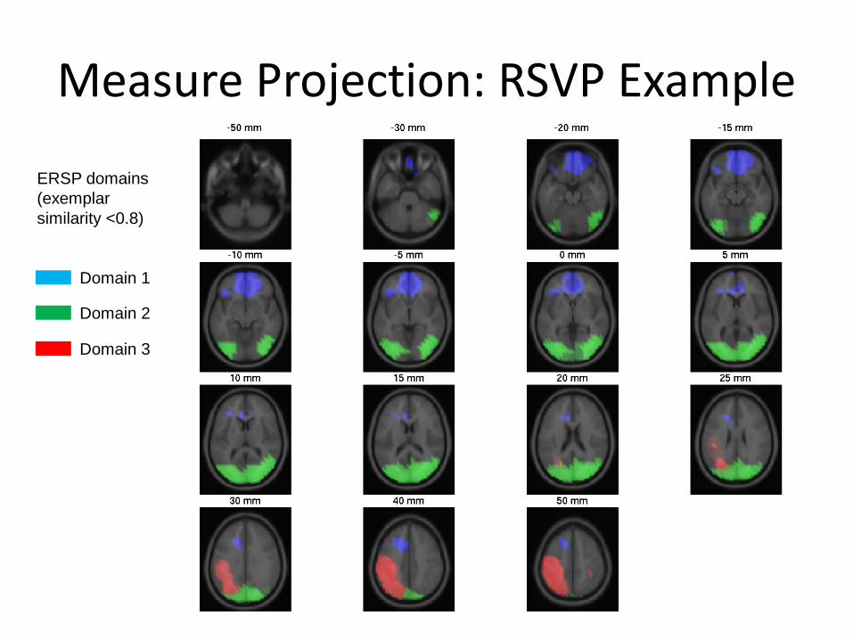
Measure Projection: RSVP Example
ERSP domains (exemplar similarity <0.8)
Domain 1
Domain 2
Domain 3
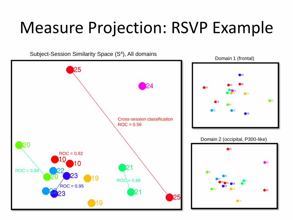
Measure Projection: RSVP ExampleSubject-Session Similarity Space (S4), All domains
Domain 1 (frontal)
Domain 2 (occipital, P300-like)
Cross-session classification ROC = 0.56
ROC = 0.88
ROC = 0.92
ROC = 0.95
ROC = 0.84
Measure Projection: Summary• Enables us to compare subjects, groups and
conditions at every brain location.• Enables us to calculate significance on every step.• Enables us to perform new types of analysis that
we could not do with IC clusters (e.g. subject similarity space)
• All types of analysis that can be done on IC clusters, can also be performed in Measure Projection framework.

Measure Projection: Summary• Assigns measures directly to brain location. This simplifies
comparing results across different studies and modalities (e.g. fMRI).
• Provides a framework for analyzing EEG data that has several advantages over clustering and does not suffer from its conceptual and practical problems.
• The closest concept in MPA to a cluster is a Domain, which identifies a region of brain volume with highly similar projected measure.

Measure Projection toolbox• 95% of capabilities alternative to
clustering are currently implemented in the toolbox.
• Pair-wise comparison of Conditions or Groups is implemented .
• MRI-like visualization and analysis.• The image on the right shows areas
with significant (p<0.03) high IC ERSP similarity in their neighborhood in an RSVP experiment.
• Voxels with similar ERSP are colored similarly (with multi-dimensional scaling of projected measure to Hue)
Measure Projection toolbox
Roadmap:
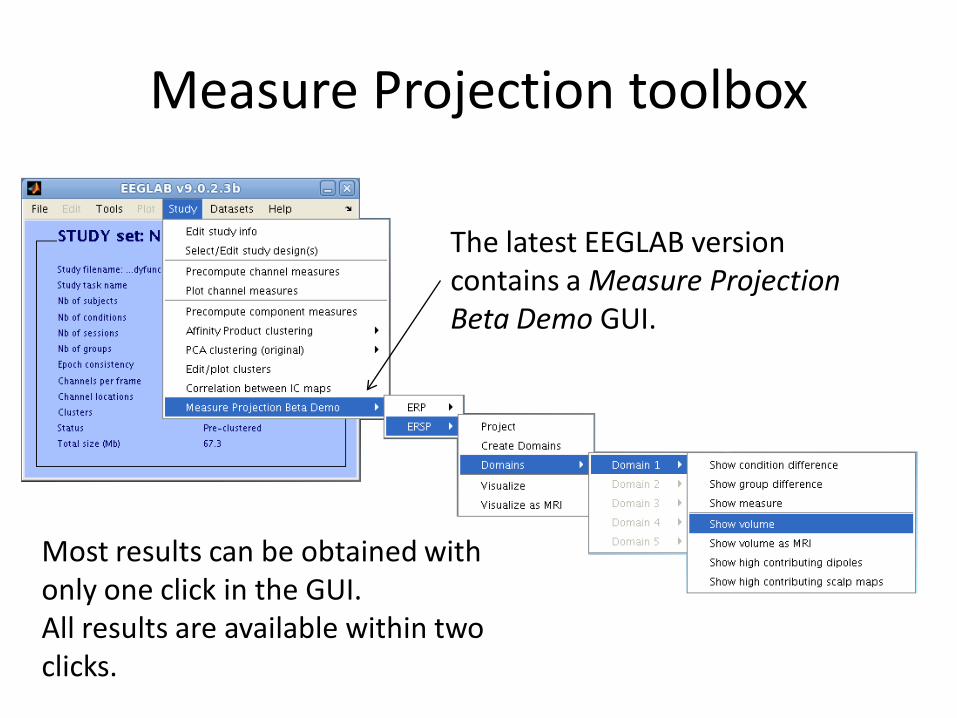
The latest EEGLAB version contains a Measure Projection Beta Demo GUI.
Most results can be obtained with only one click in the GUI.All results are available within two clicks.

Measure Projection toolbox
• Full support of STUDY Design• Single trial projection
(possibly useful for building classifier from multiple subjects)
• Multiple ICA models for each session.
• Subject-Session comparison on regions of interest (ROIs).
Roadmap:
An ERP domain from Sternberg task

Exercise: Affinity Product clustering
1. Install the latest version of EEGLAB or download, extract and copy plug-in files from the wiki to your /eeglab/plugins/ folder.
2. Type >> eeglab rebuild3. Load 5 subject N 400 study.4. Click on Study->Affinity Product clustering-> Build Pre-
clustering matrices.5. Click on Study->Affinity Product clustering-> Cluster
Components.6. Select only Dipole and ERSP measure with 10 clusters,
then click OK.

Exercise: Measure Projection clustering
1. Go to Study->Measure Projection Beta Demo -> ERSP -> Visualize
2. Try Create Domains under the ERP menu.3. Click on Domains -> Domain 1 (or n) -> Show
Volume.4. Click on Domains -> Domain 1 (or n) Show
Measure5. Try other Domain menu options.