measurement and modeling of change: just some of the issues todd d. little yale university (for...

Measurement and Modeling of Change: Measurement and Modeling of Change: Just some of the issuesJust some of the issues

Todd D. Little

Yale University (for now…)

Auburn University, May 8, 2001

OutlineOutline• Multilevel analyses

– (aka HLM; special case of SEM)

• Selecting Indicators– Parceling– Finding optimal sets

• Selecting Reporters– The case of aggression

• Missingness, Dropout, and Selectivity– What’s the diff?

• Simple Longitudinal Modeling

Multilevel StructuresMultilevel Structures• Observations at one level are nested within

observations at another

• Number of levels theoretically limitless, bounded by practicality

• Examples:– Students within classrooms, grade-level, gender

• Between subjects designs

– Persons within time of measurement• Within subjects designs

"Once you know that "Once you know that hierarchies exist, hierarchies exist,

you see them you see them everywhere."everywhere."

-Kreft and de Leeuw (1998)

Multilevel ApproachesMultilevel Approaches

• Distinguish HLM (a specific program) from hierarchical linear modeling, the technique– A generic term for a type of analysis

• Probably best to discuss MRC(M) Modeling– Multilevel Random Coefficient Modeling

• Different program implementations– HLM, MLn, SAS, BMDP, LISREL, and others

Logic of MRCMLogic of MRCM

• Coefficients describing level 1 phenomena are estimated within each level 2 unit (e.g., individual-level effects)– Intercepts—means

– Slopes—covariance/regression coefficients

• Level 1 coefficients are also analyzed at level 2 (e.g., dyad-level effects)– Intercepts: mean effect of dyad

– Slopes: effects of dyad-level predictors

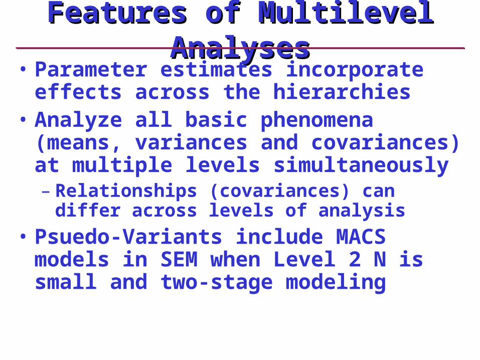
Features of Multilevel AnalysesFeatures of Multilevel Analyses• Parameter estimates incorporate effects across

the hierarchies• Analyze all basic phenomena (means, variances

and covariances) at multiple levels simultaneously– Relationships (covariances) can differ across levels

of analysis

• Psuedo-Variants include MACS models in SEM when Level 2 N is small and two-stage modeling

Group 1 Group 2 Group 3 1 8 4 13 9 18 2 7 5 12 10 17 3 6 6 11 11 16 4 5 7 10 12 15 5 4 8 9 13 14 3 6 6 11 11 16

Negative Individual, Positive GroupNegative Individual, Positive Group

Negative Individual, Positive GroupNegative Individual, Positive Group

Group 1 Group 2 Group 3 6 11 9 9 11 6 7 12 10 10 12 7 8 13 11 11 13 8 9 14 12 12 14 9

10 15 13 13 15 10 8 13 11 11 13 8

Positive Individual, Negative GroupPositive Individual, Negative Group

Positive Individual, Negative GroupPositive Individual, Negative Group

Group 1 Group 2 Group 3 1 8 4 10 9 15 2 8 5 10 10 15 3 8 6 10 11 15 4 8 7 10 12 15 5 8 8 10 13 15 3 8 6 10 11 15

No Individual, Positive GroupNo Individual, Positive Group

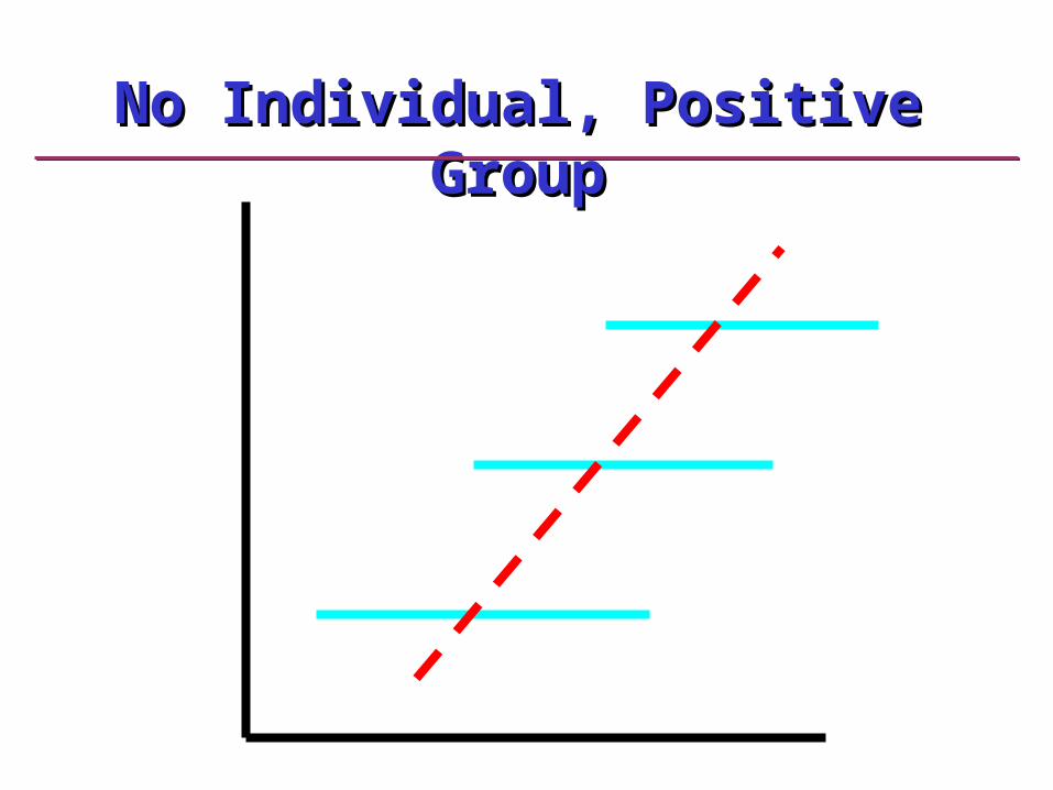
No Individual, Positive GroupNo Individual, Positive Group

No Group, Mixed IndividualNo Group, Mixed Individual

A Contrived ExampleA Contrived Example

• Yij = Friendship Closeness ratings of each

individual i within each dyad j.

• Level 1 Measures: Age & Social Skill of the

individual participants

• Level 2 Measures: Length of Friendship &

Gender Composition of Friendship dyad

The EquationsThe Equations

yij = 0j + 1jAge + 2jSocSkill + 3jAge*Skill + rij

The Level 1 Equation:

0j = 00 + 01(Time) + 02(Gnd) + 03(Time*Gnd) + u0j




The Level 2 Equations:=

Types of ConstructsTypes of Constructs

Multidimensionality

Dir

tyn

ess

Degree

of Complex

ity

Construct SpaceConstruct Space

… … and a centroidand a centroid

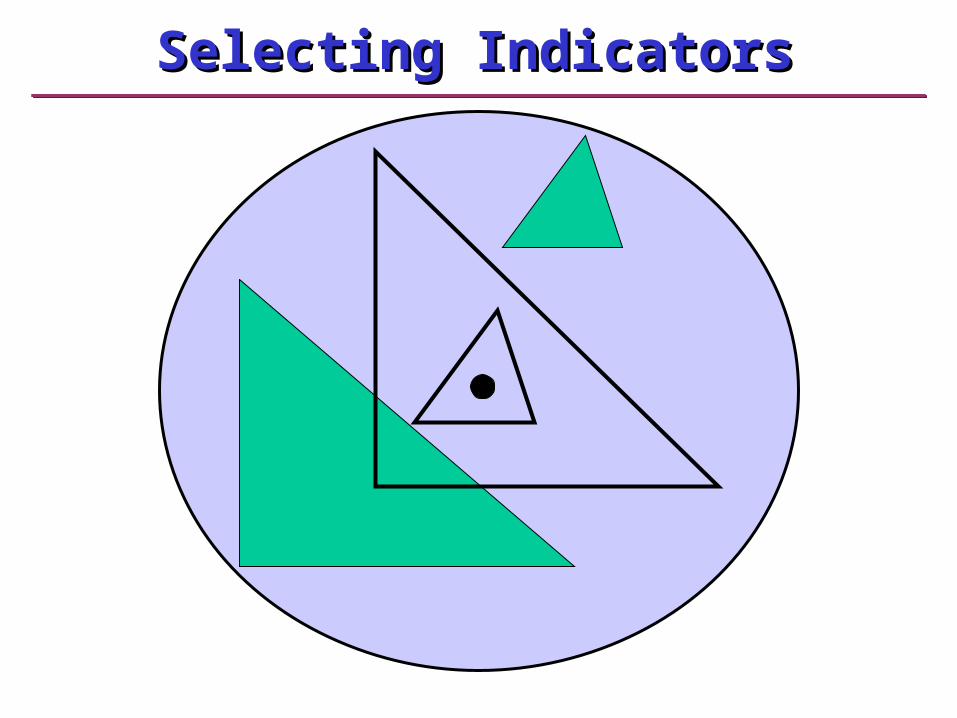
Selecting IndicatorsSelecting Indicators

Elements of the SimulationElements of the Simulation

Com

mun

alit

y

Axis of the Construct's Centroid

Maximum Reliability of an indicator (1.0)

Selection Diversity

.4

.8

.1 .3 .5

Selection Planes

Indicators of the ConstructIndicators of the Construct

Selecting Three (at random)Selecting Three (at random)

Latent Construct CentroidLatent Construct Centroid

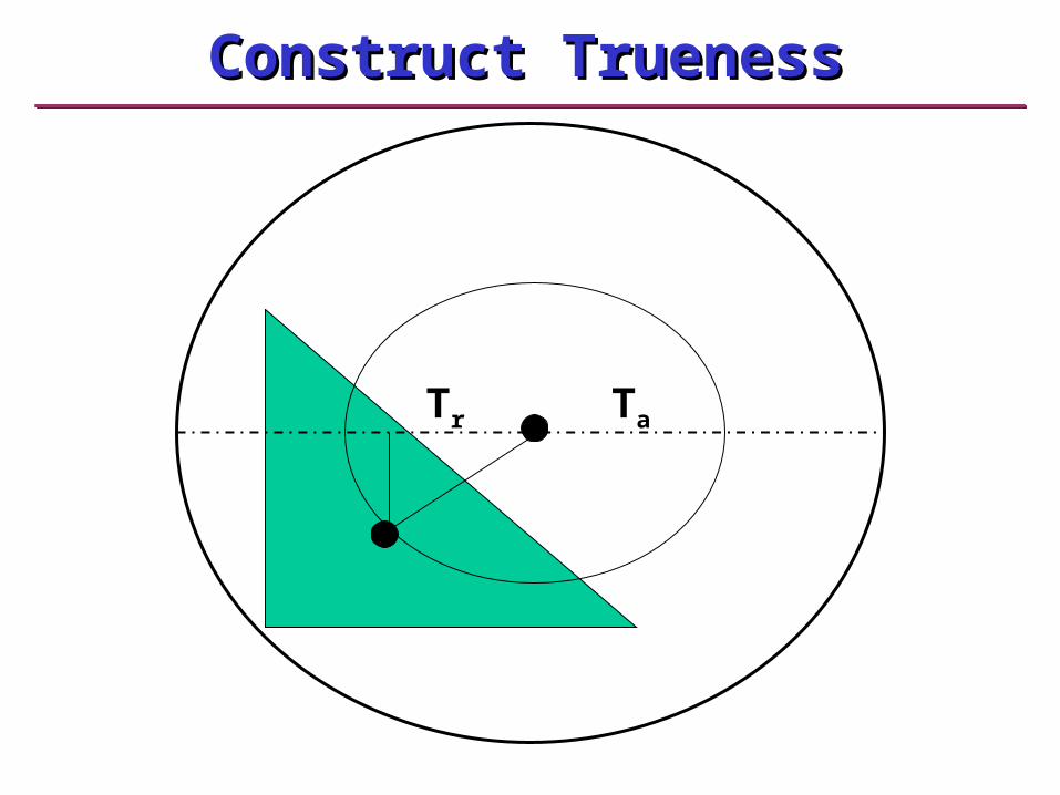
Construct TruenessConstruct Trueness

Tr Ta

… … and anotherand another

… … yet anotheryet another

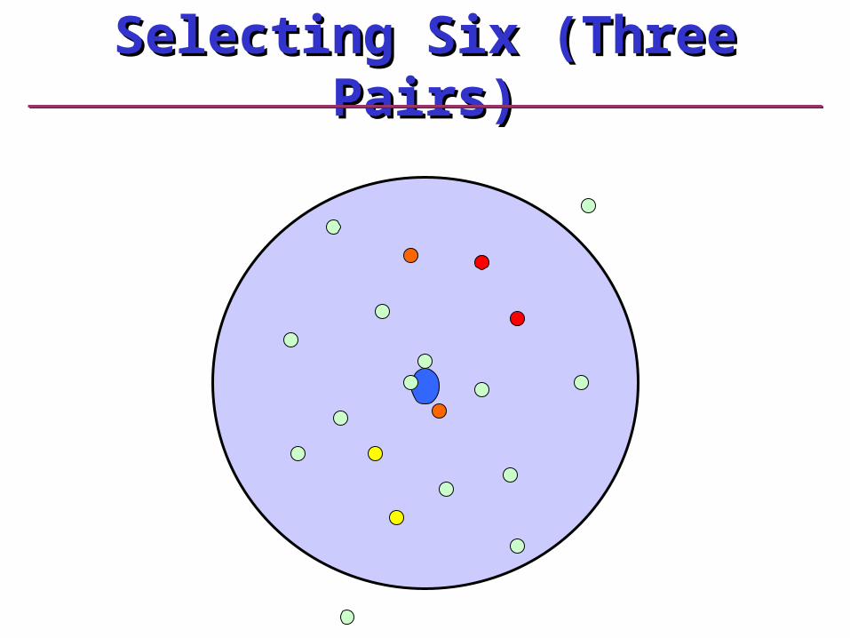
Selecting Six (Three Pairs)Selecting Six (Three Pairs)

… … take the meantake the mean

… … and find the centroidand find the centroid

How about 3 pairs of 3?How about 3 pairs of 3?

Centroid of YellowCentroid of Yellow

Centroid of RedCentroid of Red

Centroid of OrangeCentroid of Orange

… … taking the meanstaking the means

… … yields reliable & valid indictorsyields reliable & valid indictors

Construct

Specific (but reliable)

Random Error

Variance ComponentsVariance Components

+ =

Aggregate the 2 IndicatorsAggregate the 2 Indicators

+ =

Standardizing the ScaleStandardizing the Scale

A Word (picture?) of CautionA Word (picture?) of Caution

+ =+

+ =+

+ =+

} 50%

} 50%

} 50%

What is this Construct?

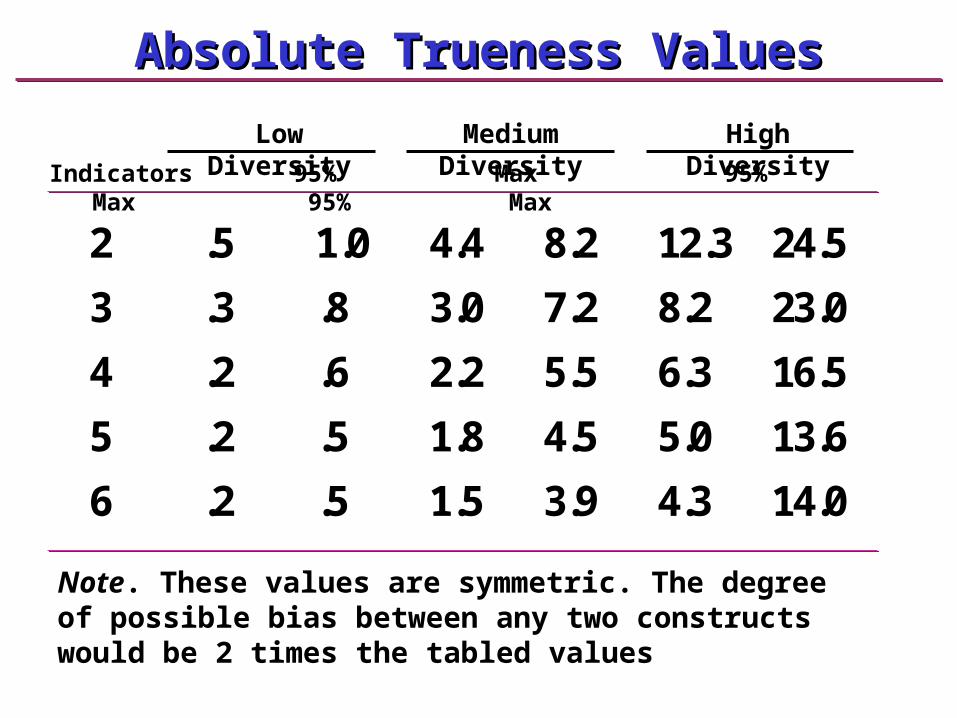
Absolute Trueness ValuesAbsolute Trueness Values

2 .5 1.0 4.4 8.2 12.3 24.5

3 .3 .8 3.0 7.2 8.2 23.0

4 .2 .6 2.2 5.5 6.3 16.5

5 .2 .5 1.8 4.5 5.0 13.6

6 .2 .5 1.5 3.9 4.3 14.0

Indicators 95% Max 95% Max 95% Max

Low Diversity Medium Diversity High Diversity

Note. These values are symmetric. The degree of possible bias between any two constructs would be 2 times the tabled values

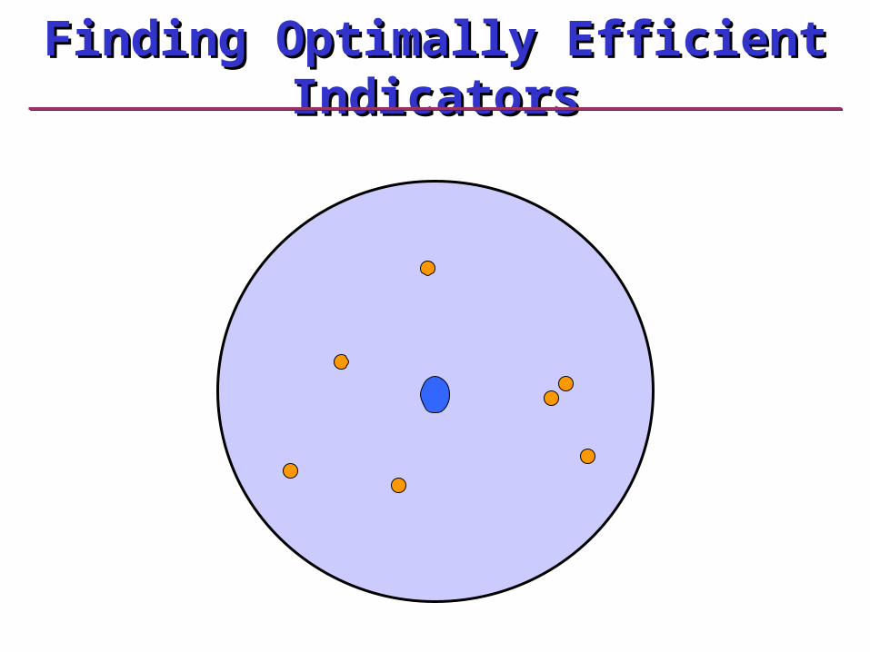
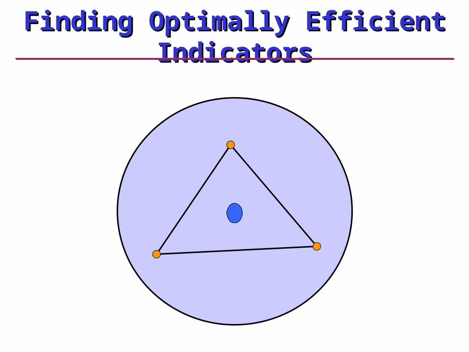
Finding Optimally Efficient IndicatorsFinding Optimally Efficient Indicators

Implications of SelectionImplications of Selection

• Confirmatory Analyses are very good.

–Little or no evidence of bias

–Doesn't overcorrect for measurement error

• You can have validity without reliability

–Hard to argue, but possible

–Need very good theory

• Don't "just do it," think about it first…

–Facilitates making better selections

–Avoids the allure of the 'bloated specific'

How To Find Them?How To Find Them?• Focus on Construct Space! Not item space.Focus on Construct Space! Not item space.

– 1) Select a broad set of constructs1) Select a broad set of constructs• Some with Small, Medium, & Large Positive CorrelationsSome with Small, Medium, & Large Positive Correlations

• Some with Small, Medium, & Large Negative CorrelationsSome with Small, Medium, & Large Negative Correlations

• Some that are zero CorrelatedSome that are zero Correlated

– 2) Calculate Latent Correlations on whole sample (save)2) Calculate Latent Correlations on whole sample (save)

– 3) Split sample into two random halves3) Split sample into two random halves

– 4) Find Optimal Set on 14) Find Optimal Set on 1stst Half of Sample Half of Sample• Systematically select all possible combinations of Systematically select all possible combinations of nn items from the items from the

original item pooloriginal item pool

• Determine the best set that reproduces whole sample correlationsDetermine the best set that reproduces whole sample correlations

– 5) Cross-validate on Second Half5) Cross-validate on Second Half

– 6) Repeat by generating on 26) Repeat by generating on 2ndnd half and cross-validating. half and cross-validating.

Inter-Reporter RelationsInter-Reporter Relations Self Friend Peer Teacher Parent

1.0

.84 1.0

.19 .17 1.0

.18 .24 .95 1.0

.31 .20 .25 .21 1.0

.21 .21 .15 .20 .72 1.0

.24 .19 .24 .17 .52 .39 1.0

.15 .13 .16 .09 .33 .32 .86 1.0

.33 .28 .06 .11 .26 .27 .27 .23 1.0

.28 .26 .00 .07 .14 .24 .18 .18 .87 1.0

O R O R O R O R O R

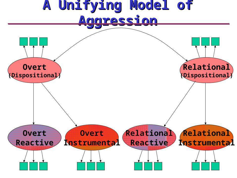
OvertReactive

OvertInstrumental

RelationalReactive

RelationalInstrumental

Overt(Dispositional)

Relational(Dispositional)

A Unifying Model of AggressionA Unifying Model of Aggression

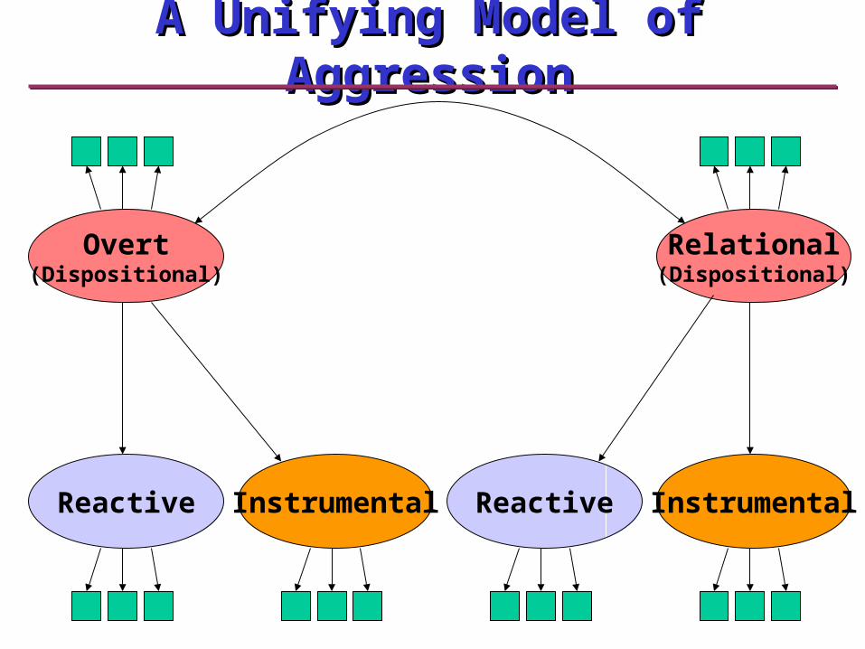
Reactive Instrumental Reactive Instrumental




Reactive Instrumental Reactive Instrumental



Reactive Instrumental




Reactive Instrumental

-.07

.83


Reactively Aggressive

Inst

rum

enta

lly

Agg

ress

ive

Neither

BothPrimarily Instrumental

Primarily

Reactive

‘Typical’ range

Sub-types of Aggression Based on FunctionSub-types of Aggression Based on Function

Dropout: Random ProcessDropout: Random Process

Time 1Time 1 Time 2Time 2 Time 3Time 3

Time 2Time 2Time 1Time 1 Time 3Time 3

Time 3Time 3Time 2Time 2Time 1Time 1

Time 2Time 2

Dropout: Functionally RandomDropout: Functionally Random


Time 1Time 1 Time 3Time 3

SelectiveSelectiveInfluenceInfluence

R = 0R = 0

Dropout: Selective Process(es)Dropout: Selective Process(es)



Survival Survival AnalysisAnalysis

Dropout Dropout AnalysisAnalysis

SelectiveSelectiveInfluenceInfluence

R = ?R = ?

Time 3Time 3Time 2Time 2

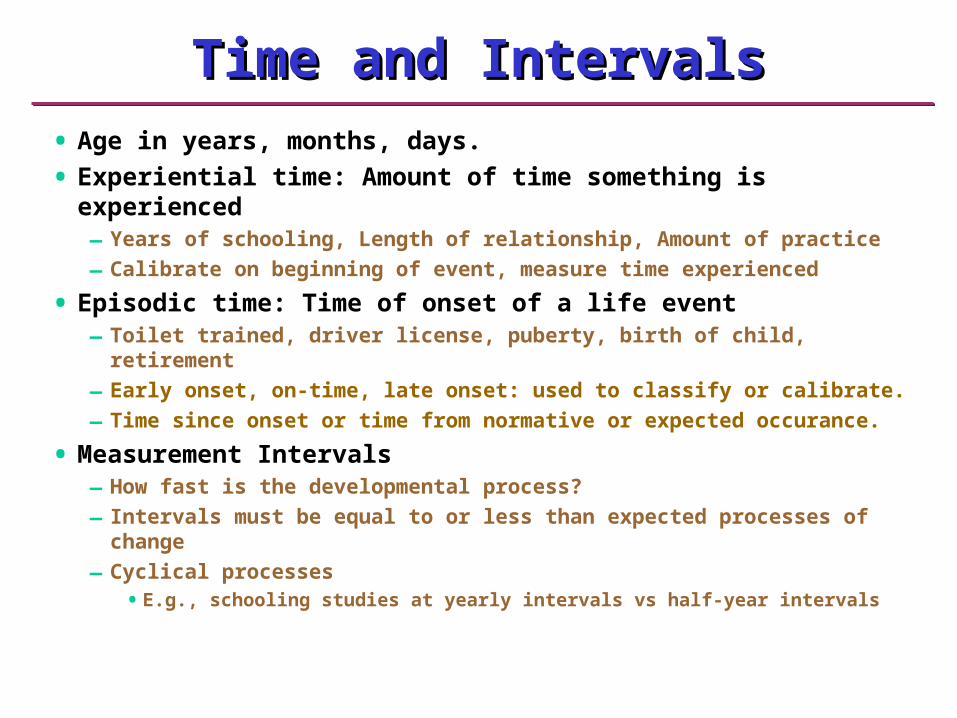
Time and IntervalsTime and Intervals

• Age in years, months, days.

• Experiential time: Amount of time something is experienced– Years of schooling, Length of relationship, Amount of practice

– Calibrate on beginning of event, measure time experienced

• Episodic time: Time of onset of a life event– Toilet trained, driver license, puberty, birth of child, retirement

– Early onset, on-time, late onset: used to classify or calibrate.

– Time since onset or time from normative or expected occurance.

• Measurement Intervals– How fast is the developmental process?

– Intervals must be equal to or less than expected processes of change

– Cyclical processes

• E.g., schooling studies at yearly intervals vs half-year intervals

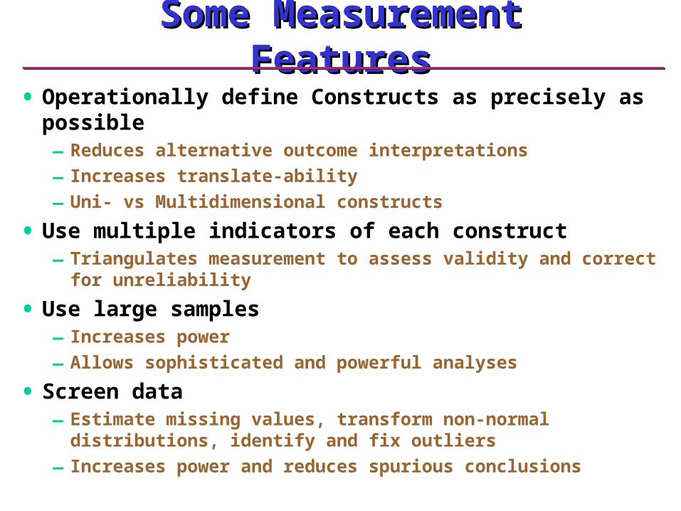
Some Measurement FeaturesSome Measurement Features

• Operationally define Constructs as precisely as possible– Reduces alternative outcome interpretations

– Increases translate-ability

– Uni- vs Multidimensional constructs

• Use multiple indicators of each construct– Triangulates measurement to assess validity and correct for

unreliability

• Use large samples– Increases power

– Allows sophisticated and powerful analyses

• Screen data– Estimate missing values, transform non-normal distributions, identify

and fix outliers

– Increases power and reduces spurious conclusions

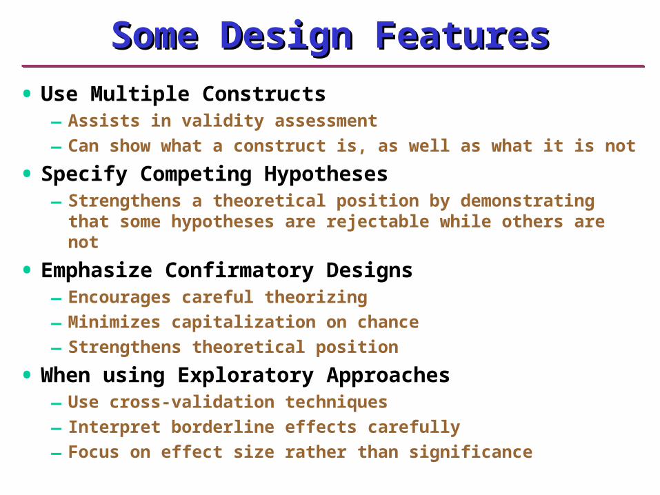
Some Design FeaturesSome Design Features

• Use Multiple Constructs– Assists in validity assessment

– Can show what a construct is, as well as what it is not

• Specify Competing Hypotheses– Strengthens a theoretical position by demonstrating that some

hypotheses are rejectable while others are not

• Emphasize Confirmatory Designs– Encourages careful theorizing

– Minimizes capitalization on chance

– Strengthens theoretical position

• When using Exploratory Approaches– Use cross-validation techniques

– Interpret borderline effects carefully

– Focus on effect size rather than significance

Some Developmental TruismsSome Developmental Truisms

• Homotypic vs heterotypic expressions

–E.g., Aggression

• Surface-structure vs deep-structure roots of behavior

–E.g., resource-directed behavior

• Different paths can lead to same outcome

• Same path can lead to different outcomes

• Development is both Qualitative & Quantitative

–Light is both wave and particle…

One construct -- Four OccasionsOne construct -- Four Occasions

Time 1Time 1 Time 2Time 2 Time 3Time 3 Time 4Time 4

e1 e2 e3 e1 e2 e3 e1 e2 e3 e1 e2 e3

Equating the reliable measurement parametersEquating the reliable measurement parameters

e4, 5, 6e7, 8, 9 e10, 11, 12

A Longitudinal Simplex StructureA Longitudinal Simplex Structure

1.0

.80 1.0

.64 .80 1.0

.51 .64 .80 1.0

T1

T2

T3

T4

Time 1 Time 2 Time 3 Time 4

Longitudinal Structures ModelLongitudinal Structures Model

Time 1Time 1 Time 2Time 2 Time 3Time 3 Time 4Time 411

2121 = = 21, 21, 3232 = = 32, 32, 4343 = = 4343

3131 = = 21213232

4141 = = 212132324343

In standardized solution, the correlations are reproduced by tracing the paths:

4242 = = 32324343

e1 e2 e3 e1 e2 e3 e1 e2 e3 e1 e2 e3

e4, 5, 6e7, 8, 9 e10, 11, 12

.8 .8 .8

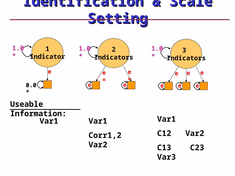
Identification & Scale SettingIdentification & Scale Setting

1Indicator

0.0*

e

1.0* 2Indicators

e e

e =e =

1.0* 3 Indicators

e e e

eee

1.0*

Var1 Var1

Corr1,2 Var2

Var1

C12 Var2

C13 C23 Var3

Useable Information:

Figural Conventions

A B

e n

Circles and Ovals represent Latent Constructs

Boxes & Rectangles represent manifest (measured) variables

Single-headed lines are directional (causal) relationships represented as regression estimates

Double-headed lines are non-directional (co-occurring) relationships represented as covariance or variance estimates

LISREL Conventions

Mn(row, column); mn(end, start) e.g. 3 from 2

When drawing, number top to bottom then left to right

1.0*

1.0*

1

2

123

456

e

eee

eee

e

e

e

e

e

e

DA NG=1 NI=6 ME=ML NO=100

KM FI=OUT_THERE.DAT

SD FI=OUT_THERE.DAT

ME FI=OUT_THERE.DAT

MO ny=6 ne=2 ly=fu,fi te=sy,fi ps=sy,fi

!note ly=ny,ne ly(indicator,construct)

Fr ly(1,1) ly(2,1) ly(3,1)

Fr te(1,1) te(2,2) te(3,3)

!note: te=ny,ny ty(indicator,indicator)

Fr ly(4,2) ly(5,2) ly(6,2)

Fr te(4,4) te(5,5) te(6,6)

!note: ps=ne,ne ps(construct,construct)

VA 1.0 ps(1,1) ps(2,2)

Fr ps(2,1)

OU so ad=off rs sc

Simple Confirmatory Factor ModelSimple Confirmatory Factor Model

3

4

789

1.0*

1.0*

e

e

e

e

e

101112

e

e

e

ee

ee

e1

2

123

1.0*

1.0*

e

eee

eee

e

e

e

456

e

e

e

A Longitudinal Confirmatory Factor ModelA Longitudinal Confirmatory Factor Model

e

e

e e


KM FI=OUT_THERE_long.DAT

SD FI=OUT_THERE_long.DAT

ME FI=OUT_THERE_long.DAT

MO ny=12 ne=4 ly=fu,fi te=sy,fi ps=sy,fi be=ze

Fr ly(1,1) ly(2,1) ly(3,1) ly(4,2) ly(5,2) ly(6,2)

Fr ly(7,3) ly(8,3) ly(9,3) ly(10,4) ly(11,4) ly(12,4)

Fr te(7,7) te(8,8) te(9,9) te(10,10) te(11,11) te(12,12)

Fr te(1,1) te(2,2) te(3,3) te(4,4) te(5,5) te(6,6)

FR te(7,1) te(8,2) te(9,3) te(10,4) te(11,5) te(12,6)

VA 1.0 ps(1,1) ps(2,2) ps(3,3) ps(4,4)

fr ps(2,1)

Fr ps(4,3)

Fr ps(3,1) ps(4,1) ps(3,2) ps(4,2)

Ou so ad=off rs sc

LISREL Source CodeLISREL Source Code

3

4

789

e

e

e

e=

e

e

e

101112

e

e

e

e=e=

e=e=

e=1

2

123

1.0*

1.0*

e

eee

eee

e

e

e

456

e

e

e

A Longitudinal Confirmatory Factor ModelA Longitudinal Confirmatory Factor Model

e

e

e e





MO ny=12 ne=4 ly=fu,fi te=sy,fi ps=sy,fi

Fr ly(1,1) ly(2,1) ly(3,1) ly(4,2) ly(5,2) ly(6,2)

Fr ly(7,3) ly(8,3) ly(9,3) ly(10,4) ly(11,4) ly(12,4)

Fr te(1,1) te(2,2) te(3,3) te(4,4) te(5,5) te(6,6)

Fr te(7,7) te(8,8) te(9,9) te(10,10) te(11,11) te(12,12)

VA 1.0 ps(1,1) ps(2,2) !ps(3,4) ps(4,4)

fr ps(2,1)

Fr ps(4,3)

Fr ps(3,1) ps(4,1) ps(3,2) ps(4,2)

LISREL Source Code: Part 1LISREL Source Code: Part 1

EQ ly(1,1) ly(7,3)

Eq ly(2,1) ly(8,3)

Eq ly(3,1) ly(9,3)

Eq ly(4,2) ly(10,4)

Eq ly(5,2) ly(11,4)

Eq ly(6,2) ly(12,4)

Fr ps(3,3) ps(4,4)

Ou so ad=off sc rs


3

4

789

e

e

e

e=

e

e

e

101112

e

e

e

e=e=

e=e=

e=1

2

123

1.0*

1.0*

e

eee

eee

e

e

e

456

e

e

e

A Longitudinal Cross-lag Structural ModelA Longitudinal Cross-lag Structural Model

e

e

e

e





MO ny=12 ne=4 ly=fu,fi te=sy,fi ps=sy,fi be=fu,fi

Fr ly(1,1) ly(2,1) ly(3,1) ly(4,2) ly(5,2) ly(6,2)

Fr ly(7,3) ly(8,3) ly(9,3) ly(10,4) ly(11,4) ly(12,4)

Fr te(1,1) te(2,2) te(3,3) te(4,4) te(5,5) te(6,6)

Fr te(7,7) te(8,8) te(9,9) te(10,10) te(11,11) te(12,12)

VA 1.0 ps(1,1) ps(2,2)

fr ps(2,1)

Fr ps(3,3) ps(4,4)

Fr ps(4,3)

!note: be=ne,ne be(construct,construct) (to,from) (row,column)

Fr be(3,1) be(4,1) be(3,2) be(4,2)


measurement and modeling of change: just some of the issues todd d. little yale university (for...

Documents