Measurement and modellingof contact stiffness

D. Nowell, University of Oxford, UK

Joints workshop, Chicago, 16/8/12

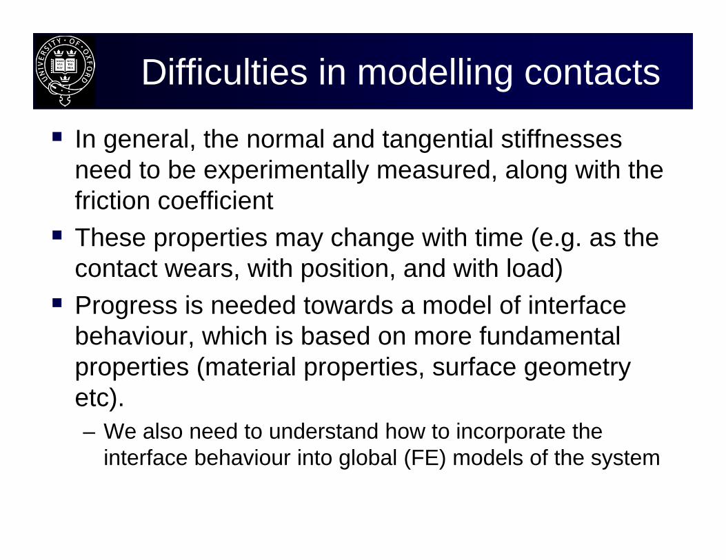
Difficulties in modelling contacts

In general, the normal and tangential stiffnessesneed to be experimentally measured, along with the friction coefficient These properties may change with time (e.g. as the

contact wears, with position, and with load) Progress is needed towards a model of interface

behaviour, which is based on more fundamental properties (material properties, surface geometry etc).– We also need to understand how to incorporate the

interface behaviour into global (FE) models of the system

Measurement of Contact behaviour –Oxford and Imperial rigs

80 mm2 flat and rounded contact

1Hz Frequency 0.6mm sliding distance Displacement

measurement by remote LVDT or digital image correlation

1 mm2 flat on flat contact

~100Hz Frequency 30m sliding distance Displacement

measurement integration of LDV measurements

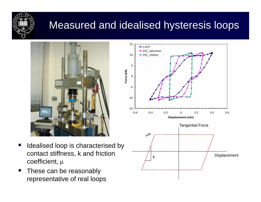
Measured and idealised hysteresis loops

Idealised loop is characterised by contact stiffness, k and friction coefficient,

These can be reasonably representative of real loops

-15

-10

-5

0

5

10

15

-0.6 -0.4 -0.2 0 0.2 0.4 0.6

Displacement (mm)

Forc

e (k

N)

LVDTDIC_specimenDIC_relative

Tangential Force

Displacementk

P

0

200

400

600

800

1000

1200

1400

1600

1800

2000

0 0.5 1 1.5 2Distance between two measured points (mm)

Con

tact

stif

fnes

s (k

N/m

m)

N=500

N=1000

N=3000

Variation of contact stiffness with measurement location

Ti ‘rough’ experiment

d

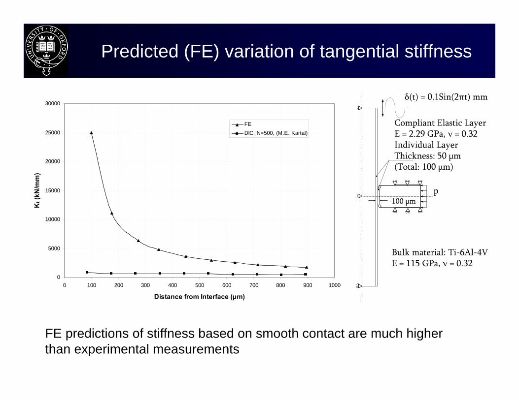
Predicted (FE) variation of tangential stiffness

0

5000

10000

15000

20000

25000

30000

0 100 200 300 400 500 600 700 800 900 1000

Distance from Interface (μm)

Kt (

kN/m

m)

FEDIC, N=500, (M.E. Kartal)

FE predictions of stiffness based on smooth contact are much higher than experimental measurements

Compliant Elastic LayerE = 2.29 GPa, ν = 0.32Individual Layer Thickness: 50 μm (Total: 100 μm)

Bulk material: Ti-6Al-4VE = 115 GPa, ν = 0.32

δ(t) = 0.1Sin(2πt) mm

100 μmp

– To develop a model for contact stiffness, we need consider surface roughness

– Initial tangential loading is likely to be predominantly elastic

– Consider a rough elastic surface in contact with a smooth rigid one. This puts all the elasticity and roughness on one surface and is easier to deal with

– At light loads, ‘asperity’ contacts will be relatively widely-spaced and may be modelled as Hertzian

Modelling - basic assumptions0

2( )

1

i

i

qq rra

2

0 1)(

arprp

– When tangentially loaded, all contacts will initially be ‘stuck’, so the shear traction at each contact will be given by

– Mindlin gives the compliance for this traction distribution as

– From this, the Greenwood/Williamson approach can be used to derive an expression for tangential stiffness

Formulation0

2( )

1

i

i

qq rra

02

( )

1

i

i

qq rra

1 1 2 1 (1 )(2 )8 4i i i iQ a G a E

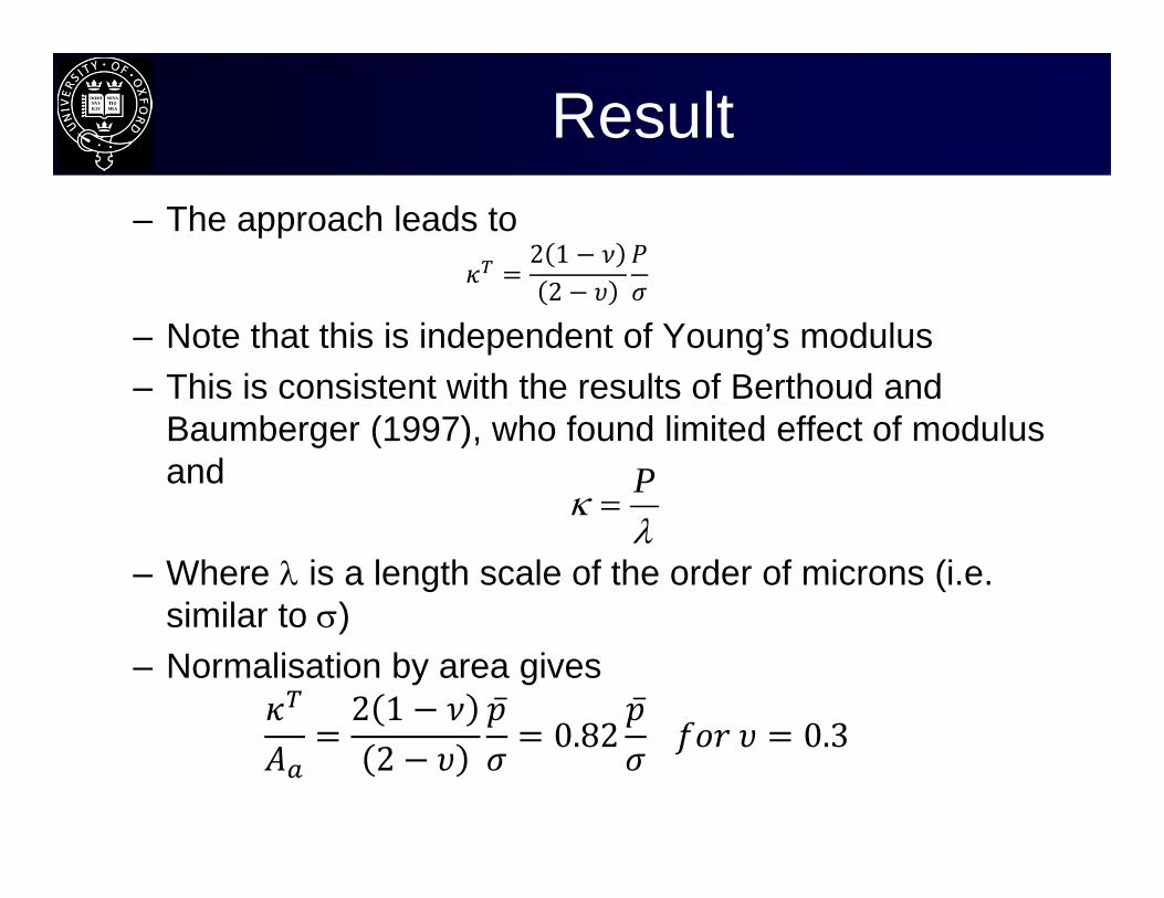
Result– The approach leads to

2 12

– Note that this is independent of Young’s modulus– This is consistent with the results of Berthoud and

Baumberger (1997), who found limited effect of modulus and

– Where is a length scale of the order of microns (i.e. similar to )

– Normalisation by area gives2 12

0.82

0.3

P

Area effect

0

200

400

600

800

1000

1200

1400

1600

0 0.2 0.4 0.6 0.8 1 1.2 1.4 1.6 1.8Distance between measured points (mm)

Tang

entia

l Con

tact

stif

fnes

s (k

N/m

m)

N 70N 400N 2017N 4520Larger area N 800Larger area N 2000Larger area N 4000

Effect of contact area on tangential contact stiffness for 70 MPa average pressure

Before normalising After normalising

Experiments carried out with different contact area do suggest that stiffness is approximately proportional to apparent area of contact

This is because almost all of the compliance is in the surface layer

Effect of normal load

Effect of normal pressure on tangential contact stiffness , N=20-25 cycles

Distance between measured points 0.18 mm

Comparison with numerical model As part of our joint

project with Imperial College, Medina has produced a numerical model of rough elastic contact

Comparison shows good agreement at low loads, but reduced stiffness in numerical model at higher loads

Effect is almost certainly caused by asperity interaction

Similar effect noted for normal contact by Ciavarella et al (2008)

0

5

10

15

20

25

30

35

40

45

0 50 100 150 200 250 300 350 400 450

Tangen

tial Stiffness (N/μm)

Load

Model

Numerical Simulation

0 1225 2450 3675Pressure (MPa)

G-VOXF

B+Binterface

111kkk smooth

Comparison with ultrasound measurements

Recent work in collaboration with Sheffield Univ has compared stiffness measured with DIC with that using ultrasound

Note that (in this case) initial value is very similar, but variation with Q is very different

Ultrasound is measuring an unloading stiffness

Ultrasound measurement Ultrasound measures an unloading stiffness:

In the case of normal stiffness, there is a similar effect, in this case there is an increase of stiffness with (normal) load and growth of the real contact area

Perspectives Tangential stiffness models should almost certainly include a

dependence on normal load.– What models are appropriate– How can we improve the models we have?– How do we capture time dependence?

Measurement of stiffness in real contacts is not straightforward.– There is a need for reconciliation between different techniques.– We cannot model what we cannot measure.

Modelling friction is far more challenging than contact stiffness– More multiphysics in this problem– Once again, time dependence is an issue– We need better models for wear

FRICTIONAL SHAKEDOWNPart 2:

16

Axis of symmetry Centreline

Grip – Fixed end

Bulk LoadT = 2t

Normal LoadP = 2ap

p

121º 121º

Pad

Speciment

2a

Punch on Half Plane with Tension

-4.5-4

-3.5-3

-2.5-2

-1.5-1

-0.50

0.51

1.52

2.5

0 0.2 0.4 0.6 0.8 1 1.2 1.4 1.6

/ p

f

0<([∆T/t] / [P/a])<1 vs. COF

-1.9<([∆T/t] / [P/a])<0 vs. COF

f = 0.296

Separation

Corner Leading Edge Partial Slip (PS)

Interior Trailing Edge PS

Interior Leading Edge PS

Fully Adhered

fcrit for 0 / p > 0

fcrit for 0 / p < 0

Simplified Model: Load vs. f Map

Incipient Interior Partial Slip

Edge Partial

Slip

Incipient Interior Partial Slip

Example Calculation Point

f = 0.296

Corner Leading Edge Partial Slip (PS)

Fully Adhered

fcrit for 0 / p > 0

fMelan – Frictional Shakedown

Simplified Model: Load vs. f Map

Probing shakedown

ProbingPoint

0

0.4

0.8

1.2

1.6

2

2.4

0 0.2 0.4 0.6 0.8 1 1.2 1.4 1.6

0 / p

f

0<([∆T/t] / [P/a])<1 vs. COF

Melan

Edge Partial

Slip fcrit for 0 / p > 0

fMelan – Frictional Shakedown Limit

Separation

Interior Cyclic Slip (PS)

Possible Frictional Shakedown Melan’s equivalent theorem

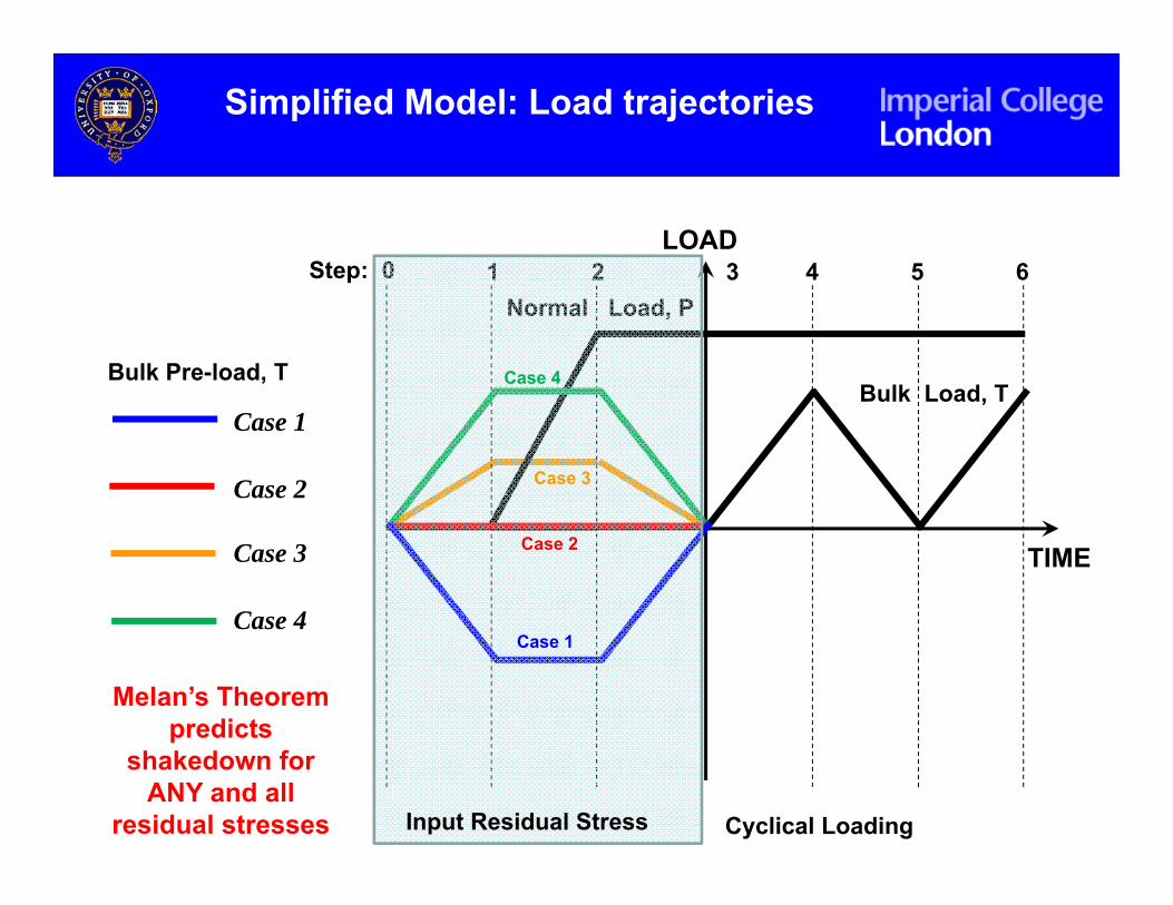
Simplified Model: Load trajectories

TIME

LOAD

Normal Load, P1 2 3 4 5 6

Bulk Load, TBulk Pre-load, T

Case 1

Case 2

Case 3

Case 4

Step: 0

Input Residual Stress Cyclical Loading

Case 1

Case 2

Case 3

Case 4

Melan’s Theorem predicts

shakedown for ANY and all

residual stresses

-1

-0.8

-0.6

-0.4

-0.2

0

0.2

0.4

0.6

0.8

1

0 0.02 0.04 0.06 0.08 0.1 0.12 0.14 0.16 0.18 0.2

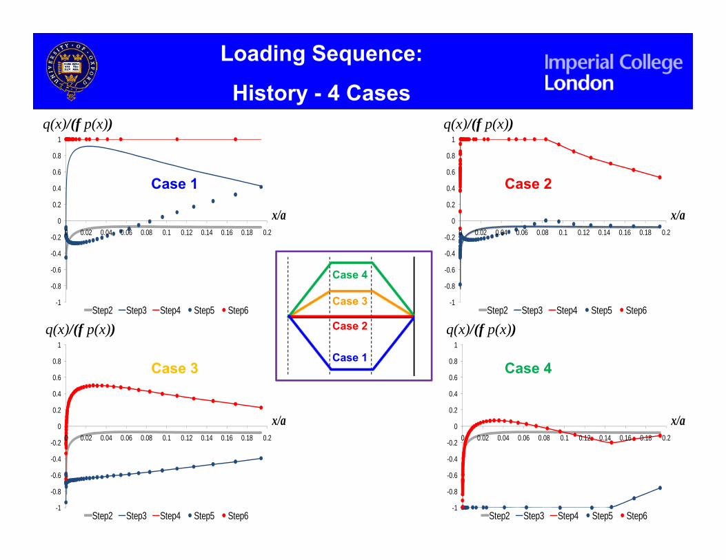
xy /( fyy )

x/a

Step2 Step3 Step4 Step5 Step6

Loading Sequence:

History - 4 Cases

-1

-0.8

-0.6

-0.4

-0.2

0

0.2

0.4

0.6

0.8

1

0 0.02 0.04 0.06 0.08 0.1 0.12 0.14 0.16 0.18 0.2

xy /( fyy )

x/a

Step2 Step3 Step4 Step5 Step6-1

-0.8

-0.6

-0.4

-0.2

0

0.2

0.4

0.6

0.8

1

0 0.02 0.04 0.06 0.08 0.1 0.12 0.14 0.16 0.18 0.2

xy /( fyy )

x/a

Step2 Step3 Step4 Step5 Step6

-1

-0.8

-0.6

-0.4

-0.2

0

0.2

0.4

0.6

0.8

1

0 0.02 0.04 0.06 0.08 0.1 0.12 0.14 0.16 0.18 0.2

xy /( fyy )

x/a

Step2 Step3 Step4 Step5 Step6

Case 1 Case 2

Case 3 Case 4

q(x)/(f p(x)) q(x)/(f p(x))

q(x)/(f p(x)) q(x)/(f p(x))

Case 1

Case 2

Case 3

Case 4

Case 2 (no pre-stress)

Does it shakedown ?

Case 2

0

1E-10

2E-10

3E-10

4E-10

5E-10

0 0.02 0.04 0.06 0.08 0.1 0.12 0.14 0.16 0.18 0.2

Slip

x/a

Step 4

Step 5

Step 6

Transient

Steady State

f = 0.296

Corner Leading Edge Partial Slip (PS)

Fully Adhered

fcrit for 0 / p > 0

fMelan – Frictional Shakedown

Simplified Model: Load vs. f Map

Probing shakedown

0

0.4

0.8

1.2

1.6

2

2.4

0 0.2 0.4 0.6 0.8 1 1.2 1.4 1.6

0 / p

f

0<([∆T/t] / [P/a])<1 vs. COF

Melan

Edge Partial

Slip fcrit for 0 / p > 0

fMelan – Frictional Shakedown Limit

Separation

Interior Cyclic Slip (PS)

Possible Frictional Shakedown Melan’s equivalent theorem

Cyclic Slip should occur above the

threshold predicted by Melan’s Theorem

ProbingPoint

Loading Sequence: Interior (?) Cyclic Slip

-1.2

-1

-0.8

-0.6

-0.4

-0.2

0

0.2

0.4

0.6

0.8

1

1.2

0 0.02 0.04 0.06 0.08 0.1 0.12 0.14 0.16 0.18 0.2

xy /( fyy )

x/a

Step2 Step3 Step4 Step5 Step6

TIME

LOAD

Normal Load, P1 2 3 4 5 6

Bulk Load, T

q(x)/(f p(x))

Loading Sequence: Interior (?) Cyclic Slip

TIME

LOAD

Normal Load, P1 2 3 4 5 6

Bulk Load, T

-2E-09

0

2E-09

4E-09

6E-09

8E-09

1E-08

1.2E-08

1.4E-08

1.6E-08

0 0.02 0.04 0.06 0.08 0.1 0.12 0.14 0.16 0.18 0.2

Slip

x/a

Step 2 Step 3 Step 4 Step 5 Step 6

Transient

Steady State

0

0.4

0.8

1.2

1.6

2

2.4

0 0.2 0.4 0.6 0.8 1 1.2 1.4 1.6

0 / p

f

0<([∆T/t] / [P/a])<1 vs. COF

Melan

f = 0.296

KIo = 0

Separation, KI o > 0

Corner Leading Edge Partial Slip (PS)

Possible Frictional Shakedown Melan’s equivalent theorem

Fully Adhered

fcrit for 0 / p > 0

fMelan – Frictional Shakedown

Interior Cyclic Slip (PS)

ProbingPoint

Simplified Model: Load vs. f Map

Probing shakedown

TIME

LOADNormal Load, P

1 2 3 4 5 6

Bulk Load, TBulk Preload, T

Case 1

Case 2

Case 3

Case 4

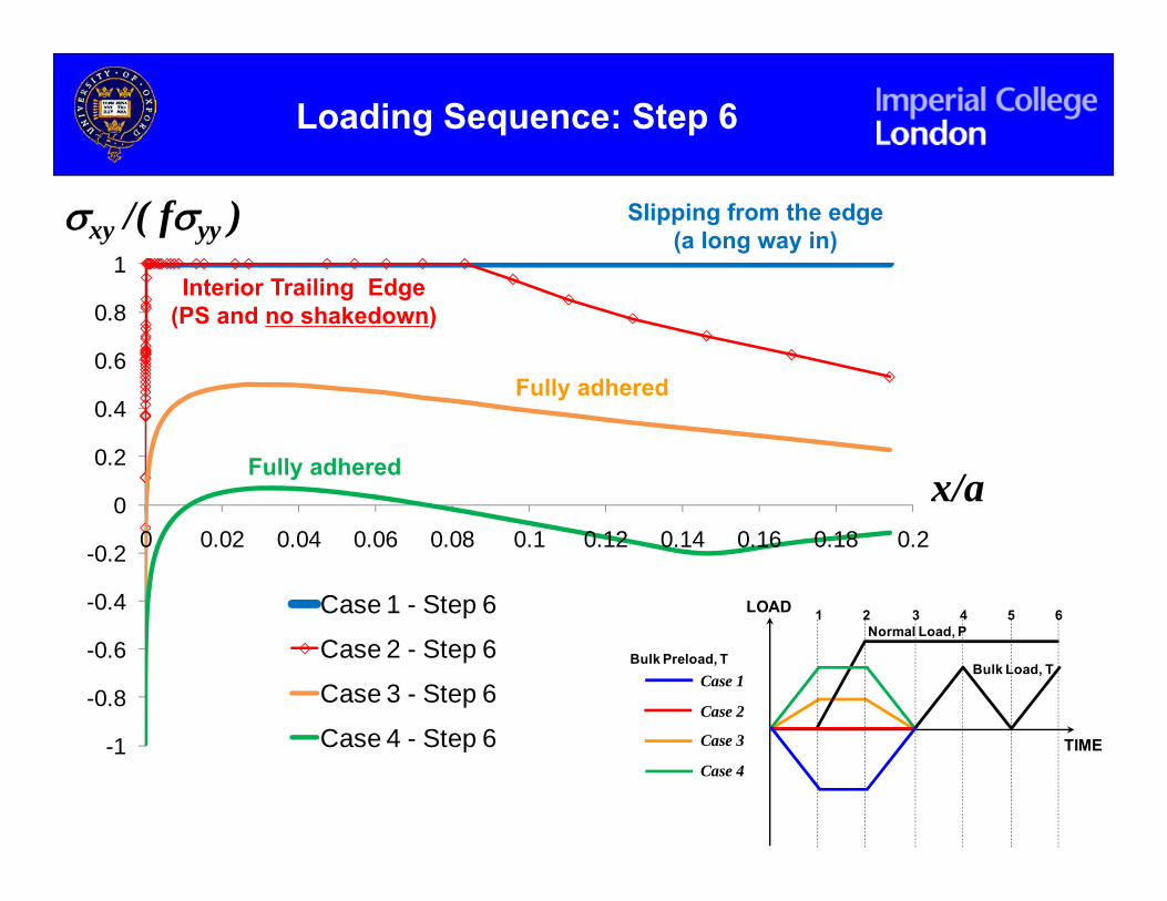
Loading scenarios designed to lock-in different sets of residual stresses

Melan’s theorem predicts frictional shakedown for

all 4 cases

-1

-0.8

-0.6

-0.4

-0.2

0

0.2

0.4

0.6

0.8

1

0 0.02 0.04 0.06 0.08 0.1 0.12 0.14 0.16 0.18 0.2

xy /( fyy )

x/a

Case 1 - Step 6

Case 2 - Step 6

Case 3 - Step 6

Case 4 - Step 6

Loading Sequence: Step 6

Slipping from the edge (a long way in)

Interior Trailing Edge (PS and no shakedown)

Fully adhered

Fully adhered

TIME

LOADNormal Load, P

1 2 3 4 5 6

Bulk Load, TBulk Preload, T

Case 1

Case 2

Case 3

Case 4