measurement and verification operational guide...measurement and verification operational guide 4...
TRANSCRIPT
Measurement and Verification Operational GuideBoilers, Steam and Compressed Air Applications

© Copyright State of NSW and Office of Environment and Heritage
With the exception of photographs, the State of NSW and Office of Environment and Heritage are pleased to allow this material to be reproduced in whole or in part for educational and non-commercial use, provided the meaning is unchanged and its source, publisher and authorship are acknowledged. Specific permission is required for the reproduction of photographs.
The Office of Environment and Heritage (OEH) has compiled this guideline in good faith, exercising all due care and attention. No representation is made about the accuracy, completeness or suitability of the information in this publication for any particular purpose. OEH shall not be liable for any damage which may occur to any person or organisation taking action or not on the basis of this publication. Readers should seek appropriate advice when applying the information to their specific needs.
Every effort has been made to ensure that the information in this document is accurate at the time of publication. However, as appropriate, readers should obtain independent advice before making any decision based on this information.
Published by: Office of Environment and Heritage NSW 59 Goulburn Street, Sydney NSW 2000 PO Box A290, Sydney South NSW 1232 Phone: (02) 9995 5000 (switchboard) Phone: 131 555 (environment information and publications requests) Phone: 1300 361 967 (national parks, climate change and energy efficiency information, and publications requests) Fax: (02) 9995 5999 TTY: (02) 9211 4723 Email: [email protected] Website: www.environment.nsw.gov.au
Report pollution and environmental incidents Environment Line: 131 555 (NSW only) or [email protected] See also www.environment.nsw.gov.au
ISBN 978 1 74293 964 3 OEH 2012/0998 December 2012
Printed on environmentally sustainable paper
Table of contents
i
Contents 1 Your guide to successful M&V projects ............................................................................ 1
1.1 Using the M&V Operational Guide ................................................................................. 1 1.2 The Boilers, Steam and Compressed Air Applications Guide (this guide) .................... 2
2 Understanding M&V concepts ........................................................................................... 4 2.1 Introducing key M&V terms ............................................................................................ 4 2.2 Best practise M&V process ............................................................................................ 5
3 Getting started ..................................................................................................................... 6 3.1 Proposed Boiler, Steam and Compressed Air ECM(s) .................................................. 6 3.2 Decide approach for pursuing M&V ............................................................................... 7
4 M&V design and planning ................................................................................................... 8 4.1 M&V design .................................................................................................................... 8 4.2 Prepare M&V plan ........................................................................................................ 14
5 Data collection, modelling and analysis ......................................................................... 17 5.1 Measure baseline data ................................................................................................. 17 5.2 Develop energy model and uncertainty ....................................................................... 20 5.3 Implement ECM(s) ....................................................................................................... 21 5.4 Measure post retrofit data ............................................................................................ 21 5.5 Savings analysis and uncertainty................................................................................. 22
6 Finish .................................................................................................................................. 24 6.1 Reporting ...................................................................................................................... 24 6.2 Project close and savings persistence ......................................................................... 24
7 M&V Examples ................................................................................................................... 25 7.1 Examples from the IPMVP ........................................................................................... 25 7.2 Examples from this guide ............................................................................................. 26
Appendix A: Example scenario A ............................................................................................ 27 Getting started ..................................................................................................................... 27 Summary of M&V plan ......................................................................................................... 28 Baseline model .................................................................................................................... 29 Calculating savings .............................................................................................................. 29 Uncertainty analysis ............................................................................................................. 29 Reporting results .................................................................................................................. 30
Appendix B: Example scenario B ............................................................................................ 31 Getting started ..................................................................................................................... 31 Summary of M&V Plan ........................................................................................................ 33 Baseline model .................................................................................................................... 34 Statistical validation of the baseline model .......................................................................... 36 Calculating savings .............................................................................................................. 37 Uncertainty Analysis ............................................................................................................ 38 Reporting results .................................................................................................................. 40


Your guide to successful M&V projects
1
1.1
1 Your guide to successful M&V projects The Measurement and Verification (M&V) Operational Guide has been developed to help M&V practitioners, business energy savings project managers, government energy efficiency program managers and policy makers translate M&V theory into successful M&V projects.
By following this guide you will be implementing the International Performance Measurement and Verification Protocol (IPMVP) across a typical M&V process. Practical tips, tools and scenario examples are provided to assist with decision making, planning, measuring, analysing and reporting outcomes.
But what is M&V exactly?
M&V is the process of using measurement to reliably determine actual savings for energy, demand, cost and greenhouse gases within a site by an Energy Conservation Measure (ECM). Measurements are used to verify savings, rather than applying deemed savings or theoretical engineering calculations, which are based on previous studies, manufacturer-provided information or other indirect data. Savings are determined by comparing post-retrofit performance against a ‘business as usual’ forecast.
Across Australia the use of M&V has been growing, driven by business and as a requirement in government funding and financing programs. M&V enables: § calculation of savings for projects that have high uncertainty or highly variable characteristics § verification of installed performance against manufacturer claims § a verified result which can be stated with confidence and can prove return on investment § demonstration of performance where a financial incentive or penalty is involved § effective management of energy costs § the building of robust business cases to promote successful outcomes
In essence, Measurement and Verification is intended to answer the question, “how can I be sure I’m really saving money?1”
1.1 Using the M&V Operational Guide The M&V Operational Guide is structured in three main parts; Process, Planning and Applications.
Process Guide: The Process Guide provides guidance that is common across all M&V projects. Practitioners new to M&V should start with the Process Guide to gain an understanding of M&V theory, principles, terminology and the overall process.
Planning Guide: The Planning Guide is designed to assist both new and experienced practitioners to develop a robust M&V Plan for your energy savings project, using a step-by-step process for designing a M&V project. A Microsoft Excel tool is also available to assist practitioners to capture the key components for a successful M&V Plan.
Applications Guides: Seven separate application-specific guides provide new and experienced M&V practitioners with advice, considerations and examples for technologies found in typical commercial and industrial sites. The Applications Guides should be used in conjunction with the Planning Guide to understand application-specific considerations and design choices. Application Guides are available for.
1 Source: www.energymanagementworld.org
Measurement and Verification Operational Guide
2
1.2
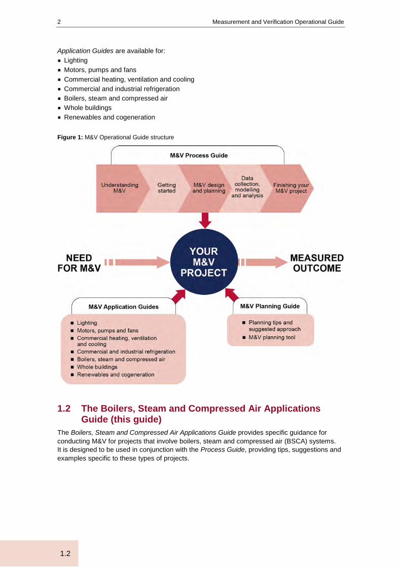
Application Guides are available for: § Lighting § Motors, pumps and fans § Commercial heating, ventilation and cooling § Commercial and industrial refrigeration § Boilers, steam and compressed air § Whole buildings § Renewables and cogeneration
Figure 1: M&V Operational Guide structure
1.2 The Boilers, Steam and Compressed Air Applications Guide (this guide)
The Boilers, Steam and Compressed Air Applications Guide provides specific guidance for conducting M&V for projects that involve boilers, steam and compressed air (BSCA) systems. It is designed to be used in conjunction with the Process Guide, providing tips, suggestions and examples specific to these types of projects.
Your guide to successful M&V projects
3
1.2
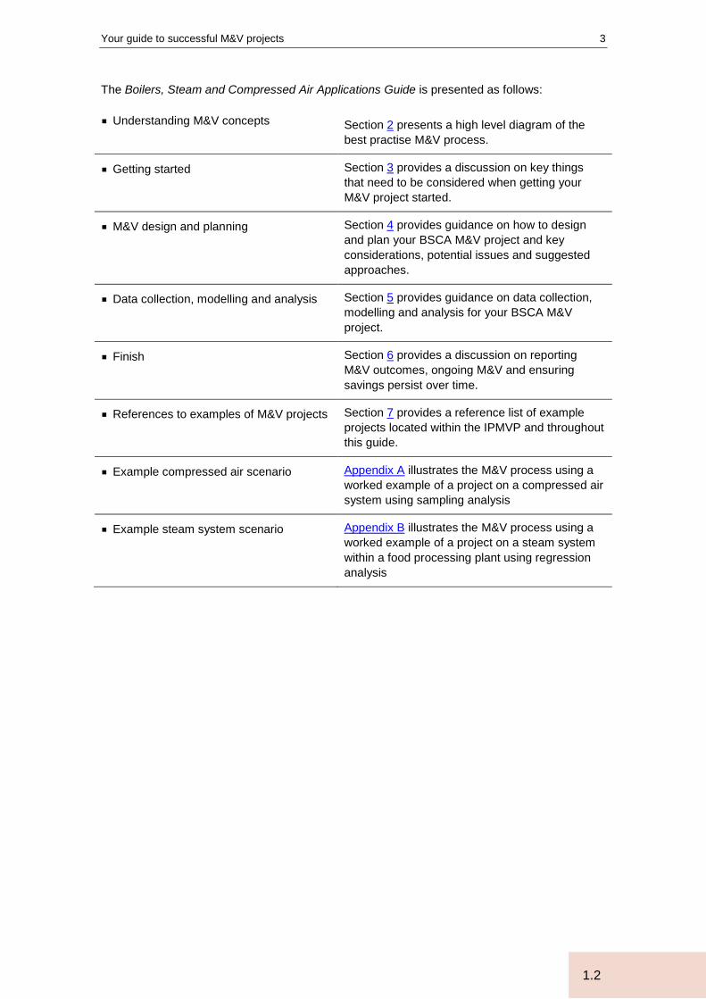
The Boilers, Steam and Compressed Air Applications Guide is presented as follows:
§ Understanding M&V concepts Section 2 presents a high level diagram of the best practise M&V process.
§ Getting started Section 3 provides a discussion on key things that need to be considered when getting your M&V project started.
§ M&V design and planning Section 4 provides guidance on how to design and plan your BSCA M&V project and key considerations, potential issues and suggested approaches.
§ Data collection, modelling and analysis Section 5 provides guidance on data collection, modelling and analysis for your BSCA M&V project.
§ Finish Section 6 provides a discussion on reporting M&V outcomes, ongoing M&V and ensuring savings persist over time.
§ References to examples of M&V projects Section 7 provides a reference list of example projects located within the IPMVP and throughout this guide.
§ Example compressed air scenario Appendix A illustrates the M&V process using a worked example of a project on a compressed air system using sampling analysis
§ Example steam system scenario Appendix B illustrates the M&V process using a worked example of a project on a steam system within a food processing plant using regression analysis
Measurement and Verification Operational Guide
4
2.1
2 Understanding M&V concepts
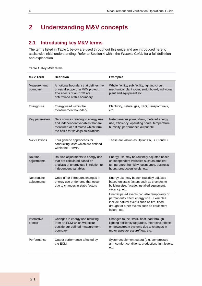
2.1 Introducing key M&V terms The terms listed in Table 1 below are used throughout this guide and are introduced here to assist with initial understanding. Refer to Section 4 within the Process Guide for a full definition and explanation.
Table 1: Key M&V terms
M&V Term Definition Examples
Measurement boundary
A notional boundary that defines the physical scope of a M&V project. The effects of an ECM are determined at this boundary.
Whole facility, sub facility, lighting circuit, mechanical plant room, switchboard, individual plant and equipment etc.
Energy use Energy used within the measurement boundary.
Electricity, natural gas, LPG, transport fuels, etc
Key parameters Data sources relating to energy use and independent variables that are measured or estimated which form the basis for savings calculations.
Instantaneous power draw, metered energy use, efficiency, operating hours, temperature, humidity, performance output etc.
M&V Options Four generic approaches for conducting M&V which are defined within the IPMVP.
These are known as Options A, B, C and D.
Routine adjustments
Routine adjustments to energy use that are calculated based on analysis of energy use in relation to independent variables.
Energy use may be routinely adjusted based on independent variables such as ambient temperature, humidity, occupancy, business hours, production levels, etc.
Non routine adjustments
Once-off or infrequent changes in energy use or demand that occur due to changes in static factors
Energy use may be non routinely adjusted based on static factors such as changes to building size, facade, installed equipment, vacancy, etc. Unanticipated events can also temporarily or permanently affect energy use. Examples include natural events such as fire, flood, drought or other events such as equipment failure, etc.
Interactive effects
Changes in energy use resulting from an ECM which will occur outside our defined measurement boundary.
Changes to the HVAC heat load through lighting efficiency upgrades, interactive effects on downstream systems due to changes in motor speed/pressure/flow, etc.
Performance Output performance affected by the ECM.
System/equipment output (e.g. compressed air), comfort conditions, production, light levels, etc.
Understanding M&V concepts
5
2.2
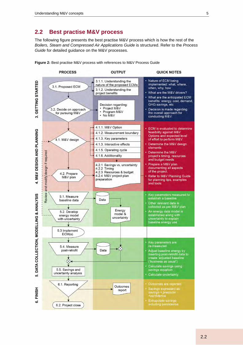
2.2 Best practise M&V process The following figure presents the best practise M&V process which is how the rest of the Boilers, Steam and Compressed Air Applications Guide is structured. Refer to the Process Guide for detailed guidance on the M&V processes.
Figure 2: Best practise M&V process with references to M&V Process Guide
Measurement and Verification Operational Guide
6
3.1
3 Getting started
3.1 Proposed Boiler, Steam and Compressed Air ECM(s)
3.1.1 BSCA projects BSCA projects aim to reduce demand and/or energy use through:
Boilers and steam generators (a) introducing or adjusting controls to properly match boiler demand and to minimise hours of
operation and wastage (b) designing and selecting energy efficient plant and equipment (c) optimising the boiler blowdown rate and control (d) installing heat recovery systems to utilise the low-grade waste heat in other applications (e) eliminating steam leaks and steam trap losses (f) minimising boiler/steam generator heat loss through better insulation (g) combinations of all of the above.
Compressed air systems (a) air leakage management and leak repairs (b) lowering the intake air temperature (c) lowering the delivery pressure (d) installation of variable speed drives (VSD’s) (e) introducing or adjusting controls to properly match air compressor demand and to minimise
hours of operation and wastage (f) designing and selecting energy efficient plant and equipment (g) installing heat recovery systems to utilise the low-grade waste heat in other applications (h) combinations of all of the above.
3.1.2 Key points to note When considering M&V it is important to understand the nature of the site and proposed ECM(s) (what, where, when, why, how much) and the project benefits (e.g. energy, demand, greenhouse gas and cost savings). Key points to note when getting started are:
§ All options are available, however Option A or Option B are most typical due to the relative size of savings in relation to site use. § It is important to understand the nature and variability of the system load to determine if it
must be measured or can be estimated. § The nature of the ECM is also important. Efficiency changes require measurement of
changes in energy use, whilst system related ECMs (e.g. leak reduction) require measurement of changes in system load. § An Option A approach may involve a system load test, combined with estimation of the
annual system load curve. § An Option B approach will involve measuring both input energy and system load and
modelling to determine the equipment’s efficiency curve. § Option C may be available for large scale systems or where multiple ECMs are being
implemented. § Determine the desired level of uncertainty (precision + confidence). § Determine the required and desirable M&V outcomes.

Getting started
7
3.2
§ The length of measurement is determined by the chosen option, and the desired level of accuracy.
Section 4.2 provides detailed information on other M&V considerations for BCSA projects.
3.2 Decide approach for pursuing M&V Once the nature of the M&V project is scoped and the benefits assessed, the form of the M&V can be determined. Decide which M&V approach you wish to pursue: 1. Conduct project-level M&V 2. Conduct program-level M&V using a sample based approach incorporating project level
M&V supplemented with evaluation within the program ‘population’. 3. Adopt a non-M&V approach in which savings are estimated, or nothing is done.

Measurement and Verification Operational Guide
8
4.1
4 M&V design and planning
4.1 M&V design
4.1.1 M&V Option Use the matrix below to assist with identifying your project’s key measurement parameters and guidance on choosing the appropriate M&V Option.
Table 2: Guidance on choosing the appropriate M&V Option
Typical projects M&V Option
Key parameters
To measure To estimate or stipulate
To consider
Changes in system efficiency § Replacement of individual
major plant/equipment such as a boiler.
§ Upgrading central BSCA system including redesign and/or replacement of equipment.
§ Installing heat recovery systems to utilise the low-grade waste heat in other applications and hence improve the overall operational efficiency.
§ Minimising boiler/steam generator heat loss through better insulation.
OP
TIO
N A
Changes in power draw or energy use
Operating hours Interactive effects System load
Variability and uncertainty of power draws and operating hour Consider pressure drop throughout the distribution system. Keep the point(s) of measurement consistent to ensure a like-for-like comparison
Changes in system load requirements § Compressed air leak
management and leak repairs. § Optimising the boiler blowdown
rate and control. § Eliminating steam leaks and
steam trap losses.
System load Changes in power draw or energy use
Variability and uncertainty of power draws and operating hour Consider pressure drop throughout the distribution system. Keep the point(s) of measurement consistent to ensure a like-for-like comparison
Changes in equipment operating hours § Time clocks § Push buttons § Pressure sensors
Operating hours Changes in power draw Interactive effects
System load System recharge requirement on start up Consider pressure drop throughout the distribution system. Keep the point(s) of measurement consistent to ensure a like-for-like comparison
M&V design and planning
9
4.1
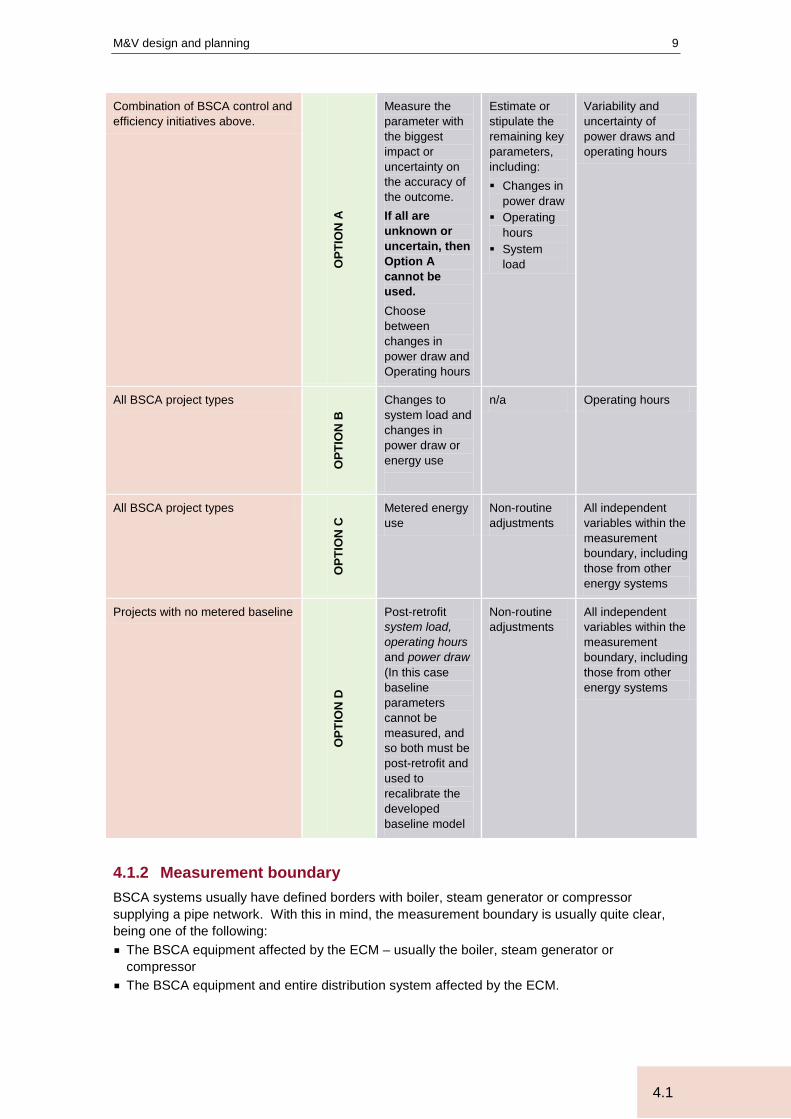
Combination of BSCA control and efficiency initiatives above.
OPT
ION
A
Measure the parameter with the biggest impact or uncertainty on the accuracy of the outcome. If all are unknown or uncertain, then Option A cannot be used. Choose between changes in power draw and Operating hours
Estimate or stipulate the remaining key parameters, including: § Changes in
power draw § Operating
hours § System
load
Variability and uncertainty of power draws and operating hours
All BSCA project types
OPT
ION
B Changes to
system load and changes in power draw or energy use
n/a Operating hours
All BSCA project types
OPT
ION
C Metered energy
use Non-routine adjustments
All independent variables within the measurement boundary, including those from other energy systems
Projects with no metered baseline
OPT
ION
D
Post-retrofit system load, operating hours and power draw (In this case baseline parameters cannot be measured, and so both must be post-retrofit and used to recalibrate the developed baseline model
Non-routine adjustments
All independent variables within the measurement boundary, including those from other energy systems
4.1.2 Measurement boundary BSCA systems usually have defined borders with boiler, steam generator or compressor supplying a pipe network. With this in mind, the measurement boundary is usually quite clear, being one of the following: § The BSCA equipment affected by the ECM – usually the boiler, steam generator or
compressor § The BSCA equipment and entire distribution system affected by the ECM.

Measurement and Verification Operational Guide
10
4.1
§ The BSCA equipment, distribution system, as well as the end-use equipment and/or production processes that control the need for hot water, steam or compressed air. This may be most appropriate where significant variations in system load occur due to variable production modes, product mix or shifts.
For example, consider a typical compressed air system. Compressed air systems range in size however they typically consist of the following components: 1. Air compressors 2. Aftercoolers and moisture separators and air dryers 3. Air receivers (compressed air storage tanks) 4. Filters to remove particles and compressor oil 5. Distribution lines 6. End use equipment
A typical compressed air system is shown in Figure 3.
Figure 3: Components of a typical compressed air system
Depending on our project and the option we select, we may consider one of the three measurement boundaries described earlier.
Air intake filter
Air compressor(s) After cooler Moisture
separator Air receiver
Air dryer Particle filter
Oil removal
filter
Sec
onda
ry
lines
Sec
onda
ry
lines
Sec
onda
ry
lines
Main distribution line
Equipment loads
Equipment loads
Equipment loads
Removes particulates
Compresses intake air
Cools the air to remove entrapped water vapour
Large storage tank which acts as a buffer
between the fluctuating air demand from the system load and the
compressor
Final stage of air drying and filtering to deliver high quality air to distribution system
Com
pres
sed
air p
lant
(s
uppl
y si
de)
Dis
tribu
tion
and
syst
em lo
ad
(dem
and
side
)
Input Energy
Input Air (moisture and temperature)
Compressed Air (pressure and
volume)

M&V design and planning
11
4.1
It is important to review the nature of the project when choosing the measurement boundary, to ensure that all affected components are included in the boundary. In addition it is important to identify the key parameters to be measured, and where they will be measured.
BSCA systems experience pressure and/or temperature drop throughout the distribution system. Keep the point(s) of measurement consistent to ensure a like-for-like comparison
4.1.3 Key parameters The table below lists the key parameters to be considered when conducting M&V for a BSCA efficiency project.
Table 3: Key parameters to be considered when conducting M&V for BSCA projects
Parameter Description
Power draw or input energy
For BSCA efficiency retrofit projects, the change in the power draw or energy use may be a key parameter to measure depending on the variability of the system load requirements, operating hours and associated uncertainty. Power draw should be measured for ECMs involving an efficiency change between energy use and system load requirements. It may be measured or estimated (using Option A) for ECMs that involve changes to system load. The power draw is usually expressed in kilowatts (kW) whilst energy use is expressed in kilowatt-hours (kWh). When replacing equipment or installing/modifying controls which result in more efficient operation of the BSCA plant, measuring the power draw may not be a straight forward exercise as it may vary considerably due to independent variables.
Compressed air intake air temperature Or Boiler feedwater temperature
In some ECMs, changes are made at the central plant to optimise the input ‘medium’ in order to reduce energy use. In compressed air systems, this may involve adding air intake ductwork to source fresh air from outside. Cooler intake air has a higher density and produces a higher volume of compressed air. In boiler and steam systems, the temperature of the boiler feedwater may be increased by harnessing waste heat or condensate return.
Operating hours This is the amount of time during which the BSCA system operates. Operating hours may be manually controlled by staff or through the use of automated controls, sensors and timers. Operating hours are dictated by the installed controls and subsequent operating patterns of the BSCA, which are influenced by one or more of the following: § Site/plant occupancy times – business hours, 24/7 operation, seasonality, public
holidays. § Daily plant process/operational requirements and associated seasonality § Type, placement and use of controls and automatic timers. § Weather/climatic seasonality. § Staff culture and behaviour. For BSCA control projects which reduce plant run-times, the change in operating hours may be a suitable key parameter to measure depending on the variability of the power draw and associated uncertainty. For simplified M&V within BSCA retrofit projects which result in a reduction of a static load (e.g. reduced compressed air supply pressure), operating hours may be assumed constant, but once again this will depend on the variability of the operating hours and associated uncertainty.
Measurement and Verification Operational Guide
12
4.1
Parameter Description
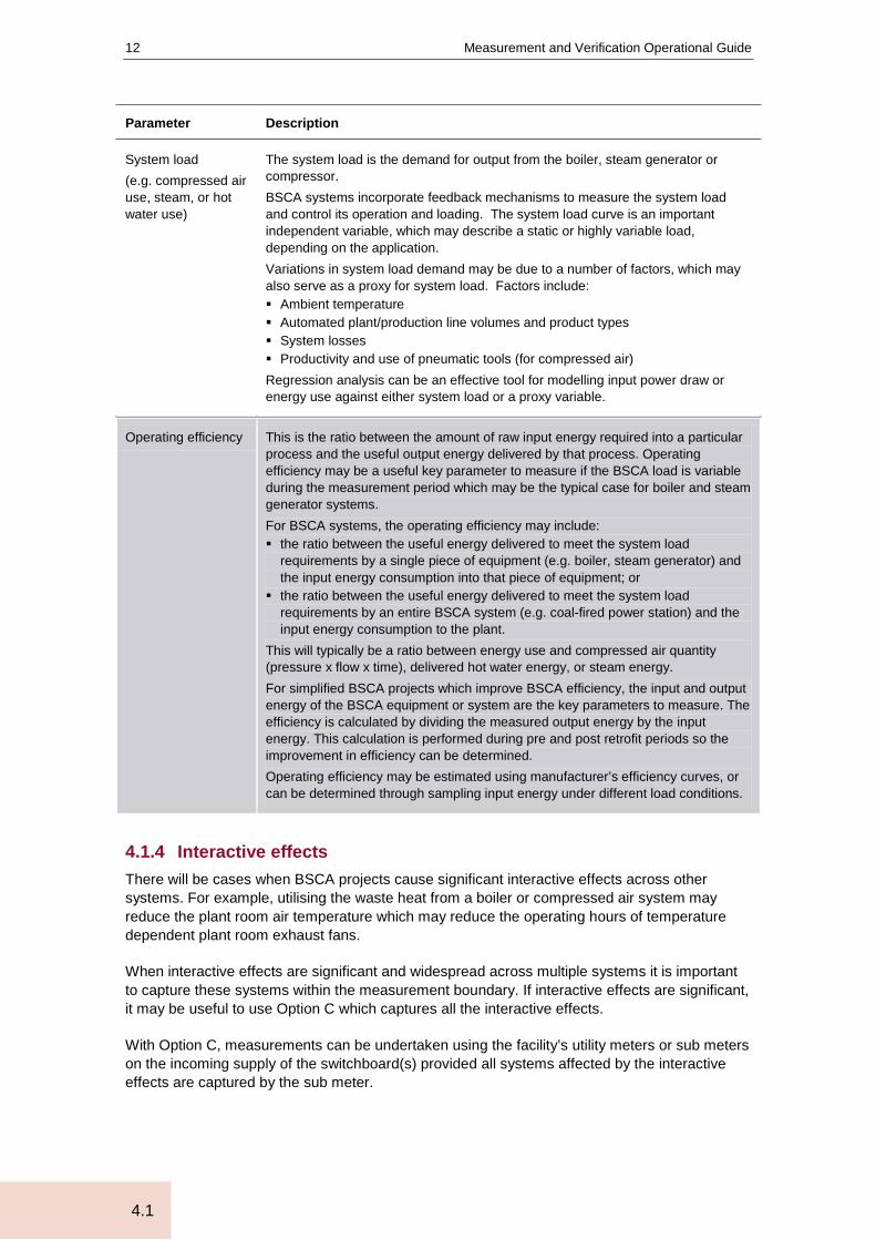
System load (e.g. compressed air use, steam, or hot water use)
The system load is the demand for output from the boiler, steam generator or compressor. BSCA systems incorporate feedback mechanisms to measure the system load and control its operation and loading. The system load curve is an important independent variable, which may describe a static or highly variable load, depending on the application. Variations in system load demand may be due to a number of factors, which may also serve as a proxy for system load. Factors include: § Ambient temperature § Automated plant/production line volumes and product types § System losses § Productivity and use of pneumatic tools (for compressed air) Regression analysis can be an effective tool for modelling input power draw or energy use against either system load or a proxy variable.
Operating efficiency This is the ratio between the amount of raw input energy required into a particular process and the useful output energy delivered by that process. Operating efficiency may be a useful key parameter to measure if the BSCA load is variable during the measurement period which may be the typical case for boiler and steam generator systems. For BSCA systems, the operating efficiency may include: § the ratio between the useful energy delivered to meet the system load
requirements by a single piece of equipment (e.g. boiler, steam generator) and the input energy consumption into that piece of equipment; or
§ the ratio between the useful energy delivered to meet the system load requirements by an entire BSCA system (e.g. coal-fired power station) and the input energy consumption to the plant.
This will typically be a ratio between energy use and compressed air quantity (pressure x flow x time), delivered hot water energy, or steam energy. For simplified BSCA projects which improve BSCA efficiency, the input and output energy of the BSCA equipment or system are the key parameters to measure. The efficiency is calculated by dividing the measured output energy by the input energy. This calculation is performed during pre and post retrofit periods so the improvement in efficiency can be determined. Operating efficiency may be estimated using manufacturer’s efficiency curves, or can be determined through sampling input energy under different load conditions.
4.1.4 Interactive effects There will be cases when BSCA projects cause significant interactive effects across other systems. For example, utilising the waste heat from a boiler or compressed air system may reduce the plant room air temperature which may reduce the operating hours of temperature dependent plant room exhaust fans.
When interactive effects are significant and widespread across multiple systems it is important to capture these systems within the measurement boundary. If interactive effects are significant, it may be useful to use Option C which captures all the interactive effects.
With Option C, measurements can be undertaken using the facility’s utility meters or sub meters on the incoming supply of the switchboard(s) provided all systems affected by the interactive effects are captured by the sub meter.
M&V design and planning
13
4.1
Additionally, the following should be considered when using Option C: § Expected savings should exceed 10% of the baseline energy. If the expected savings is
small, consider adding additional ECMs to the M&V plan. § Utility meters can be considered 100% correct however the accuracy of non-utility meters
(e.g. sub meters) should be considered in the M&V plan together with a way of validating meter readings. § Reasonable correlations can be found between energy use and other independent variables. § A system for tracking static factors can be established to enable possible non-routine
adjustments. § Major future changes to the facility are not expected during the reporting period.
In summary, the interactive effects will be dependent on the type of BSCA ECM implemented, measurement boundary and M&V Option used. Refer to the Process Guide for more guidance on interactive effects.
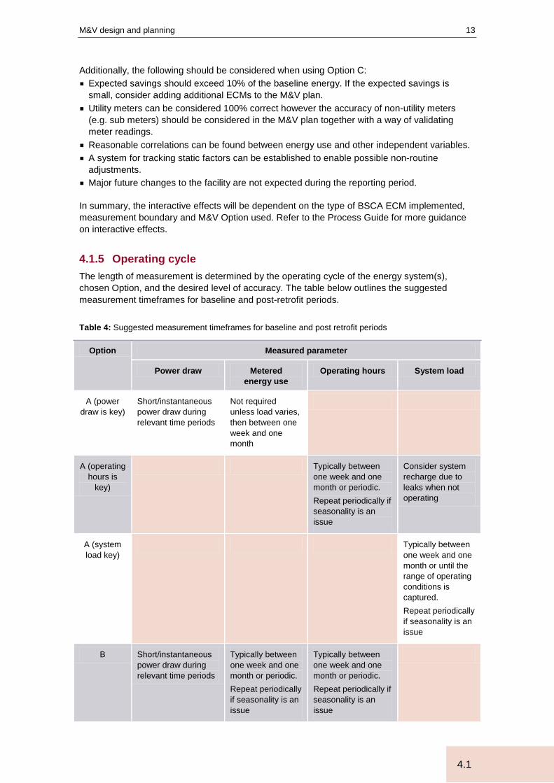
4.1.5 Operating cycle The length of measurement is determined by the operating cycle of the energy system(s), chosen Option, and the desired level of accuracy. The table below outlines the suggested measurement timeframes for baseline and post-retrofit periods.
Table 4: Suggested measurement timeframes for baseline and post retrofit periods
Option Measured parameter
Power draw Metered energy use
Operating hours System load
A (power draw is key)
Short/instantaneous power draw during relevant time periods
Not required unless load varies, then between one week and one month
A (operating hours is
key)
Typically between one week and one month or periodic. Repeat periodically if seasonality is an issue
Consider system recharge due to leaks when not operating
A (system load key)
Typically between one week and one month or until the range of operating conditions is captured. Repeat periodically if seasonality is an issue
B Short/instantaneous power draw during relevant time periods
Typically between one week and one month or periodic. Repeat periodically if seasonality is an issue
Typically between one week and one month or periodic. Repeat periodically if seasonality is an issue

Measurement and Verification Operational Guide
14
4.2
C At least one site operation ‘cycle’, that includes changes in other energy systems. For example, 12 months baseline data is required where seasonality is a factor. Typically require at least three months of post-retrofit data
At least one site operation ‘cycle’, that includes changes in other energy systems. For example, 12 months baseline data is required where seasonality is a factor. Typically require three months of post-retrofit data
D For the baseline typically one site operation ‘cycle’ is modelled. Operating hours is the key parameter in this scenario, and so short-term electrical measurement is sufficient.
For the baseline typically one site operation ‘cycle’ is modelled. Operating hours is the key parameter in this scenario, and so short-term electrical measurement is sufficient.
For the baseline typically one site operation ‘cycle’ is modelled. Within a BSCA project, a ‘cycle’ is typically two 12 months to accounted of climate seasonality. Post-retrofit measurements are used to re-calibrate the baseline model, and so both operating hours and power draw must be measured.
For the baseline typically one site operation ‘cycle’ is modelled. Within a BSCA project, a ‘cycle’ is typically two 12 months to accounted of climate seasonality.
4.1.6 Additionality Savings determined from multiple ECM projects may not be mutually exclusive. In other words, the combined savings of multiple ECMs implemented together will be less than the sum of the individual savings from ECMs if implemented in isolation from each other.
Below lists the suggested approaches to managing additionality which are described in detail in the Process Guide: 1. Adjust to isolate 2. ‘Black box’ approach 3. Ordered summation of remainders
4.2 Prepare M&V plan The next step of the M&V process is to prepare an M&V plan which is based on the M&V design and the time, resources and budget necessary to complete the M&V project.
Refer to the Planning Guide for further guidance on preparing an M&V plan.
The table below outlines issues commonly found when conducting M&V on BSCA projects and provides suggested approaches for addressing them in you M&V plan and when executing the M&V project.

M&V design and planning
15
4.2
Table 5: Considerations, issues and suggested approach for BSCA projects
Consideration Issue Suggested Approach
Measuring the reduction in power draw when the BSCA load is variable
The BSCA system does not operate at a static load. For example, the load on variable speed air compressors used for will ramp up and down depending on the system pressure. Therefore when the BSCA project is aimed at reducing the power draw without compromising the demand for BSCA (i.e. improving the operational efficiency of the BSCA system), it may not be a straightforward M&V process since you simply can’t just take instantaneous measurements of the power draw during pre and post retrofit periods like you would with lighting to calculate the reduced load.
If the BSCA project results in an improvement in operational efficiency of the BSCA system and the annual input energy consumption into the BSCA system is known and preferably recorded for more than 2 years, consider using Option A by using the BSCA operational efficiency as the key parameter to measure and stipulating the annual input BSCA energy consumption: a. Ensure the measurement boundary adequately
covers the systems affected by the project. b. Determine the base year input energy
consumption into the BSCA system from historical records and its associated uncertainty. If the uncertainty is within an acceptable range, continue to c.
c. Take measurements on the input and output energy into the BSCA system during pre and post retrofit periods.
d. Calculate the improvement in the average operational efficiency by dividing the output energy by the input energy separately for pre and post retrofit periods.
e. Ensure the measurement period is long enough to account for the normal range of operating conditions.
f. Calculate the savings by multiplying the improvement in operational efficiency with the base year input energy consumption into the BSCA system and apply the necessary uncertainty calculations.
Alternatively use Option B to continuously monitor input energy use and system load over a suitable measurement period.
Consider load and unloading components
Typically, compressors will be cycling between load conditions (e.g. reading on the outlet pressure gauge is rising) and unload conditions (e.g. reading on the outlet pressure gauge is falling).
It is important that both load and unload conditions are measured, particularly when seeking to use Option A. If the compressor is not cycling, the following procedure can be adopted to achieve load and un-load conditions: a. Full load Conditions - Open the discharge valve
from the air receiver and measure the power consumed by the compressor as it builds up pressure.
b. No-Load Conditions - Shut the valve between the air compressor and the air receiver and measure the power.

Measurement and Verification Operational Guide
16
4.2
Consideration Issue Suggested Approach
Power factor Potential changes in power factor, which might affect demand and thus cost savings. For example: motors used for mechanical air compressors will operate at different power factors depending on type, size, speed and % load.
Technology retrofits may affect the power factor within the M&V boundary, which may impact demand savings. The proposed approach is: 1. Make sure measurements are collected for real
power and/or total power, rather than simply collected readings for current only.
2. Estimate the power factor before and after the retrofit by conducting measurements or reviewing equipment specifications. If the change is minor, then its affects can be ignored. If the change is material, then:
3. Determine if the change in power factor is likely to affect overall site maximum demand (if this is an energy cost item). Does the BSCA system operate at peak demand times? Will an existing power factor correction unit negate this issue?
4. If maximum demand is affected, then apply the appropriate demand cost rates to calculate the financial impact.
Persistence and extrapolation
The savings calculated from short-term measurements often extrapolated to ‘estimate’ annual project savings. It is important to incorporate additional factors, which may include: § reliance on human
behaviour § seasonal effects (climate,
holidays, etc) § calibration changes and
failures § likelihood of future changes
within measurement boundary.
When extrapolating the savings verified during the post-retrofit period to estimate annual savings, it is important to identify influencing factors and assess their impact. If minor, they can be ignored. If material, the M&V plan should document how they are to be addressed. Examples include: a. repeating M&V at various times throughout the
year b. collecting appropriate data (such as site closure
dates and public holidays) and adjusting accordingly
c. combining short-term measurement of load with more periodic measurement of control (e.g. human behaviour)
d. occasional spot measurements to verify assumptions.
Data collection, modelling and analysis
17
5.1
5 Data collection, modelling and analysis
5.1 Measure baseline data
5.1.1 Determine existing BSCA inventory If not already done, catalogue the baseline BSCA inventory, including: § Plant and equipment types and quantities § kW and efficiency ratings (e.g. COP) § Operation times § Controls, such as sensors or time switches and their set points § Brief description of plant layout and system redundancy
The inventory may be best represented in a spreadsheet. A system diagram may assist with documenting the measurement boundary and for selecting the appropriate placement for measurement equipment.
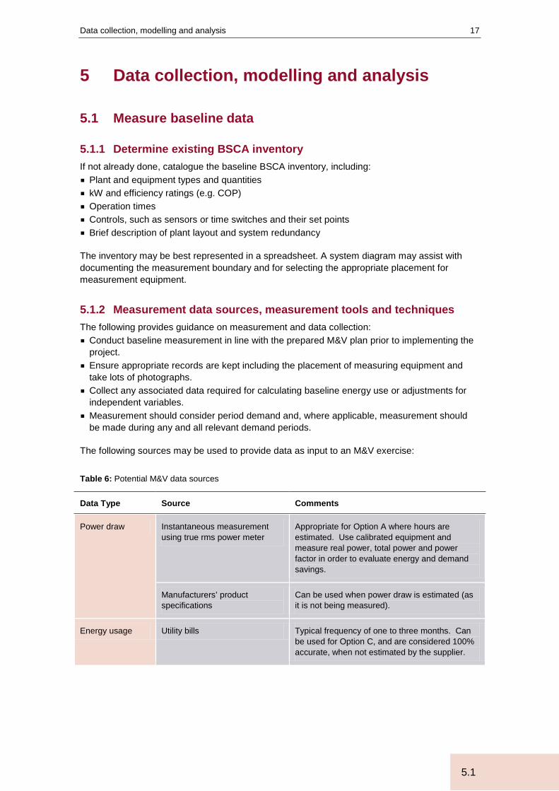
5.1.2 Measurement data sources, measurement tools and techniques The following provides guidance on measurement and data collection: § Conduct baseline measurement in line with the prepared M&V plan prior to implementing the
project. § Ensure appropriate records are kept including the placement of measuring equipment and
take lots of photographs. § Collect any associated data required for calculating baseline energy use or adjustments for
independent variables. § Measurement should consider period demand and, where applicable, measurement should
be made during any and all relevant demand periods.
The following sources may be used to provide data as input to an M&V exercise:
Table 6: Potential M&V data sources
Data Type Source Comments
Power draw Instantaneous measurement using true rms power meter
Appropriate for Option A where hours are estimated. Use calibrated equipment and measure real power, total power and power factor in order to evaluate energy and demand savings.
Manufacturers’ product specifications
Can be used when power draw is estimated (as it is not being measured).
Energy usage Utility bills Typical frequency of one to three months. Can be used for Option C, and are considered 100% accurate, when not estimated by the supplier.

Measurement and Verification Operational Guide
18
5.1
Data Type Source Comments
Energy usage Revenue meter – interval data Typically 30 minute data intervals, which can be used to accurately calculate savings across a day, week or longer. Can also be used to estimate operating hours based on profile changes. Data provided by a Meter Data Agent is used for billing and is considered 100% accurate.
Permanent sub-meter – interval data
Similar characteristics to the revenue meter above. Data quality will be high, but may not be revenue quality. Data should be reviewed for meter ‘drop outs’.
Temporary energy logger Similar to a sub-meter, an energy data logger is connected to a circuit and acts as a temporary meter. Data quality depends on the quality, range and an accuracy of the logger and associated CTs. Some units experience difficulties capturing large changes in loads. Be careful to size the CTs for the load to be measured. A tong reading will assist with sizing, however all operating loads should be considered. Also consider the effects of power factor. Simultaneously measure current and voltage using a power meter logger.
Manual meter readings (e.g. hourly/daily)
Periodic manual readings of a revenue/sub-meter. Take care to read the meter in the correct way and apply any meter multiplier ‘k factor’ to the values if stated on the meter. Contact the electricity supplier if unsure how to read the meter.
Operating hours Security system records (access swipe cards)
Time stamped records may be available from security systems, which may assist with tracking occupancy and operating patterns.
BSCA control schedules/settings (e.g. time clocks, SCADA systems, run on time settings)
Fixed or logic based time schedules that are in place for the BSCA system. This simply involves interrogating the BSCA control equipment to extract the operating schedules.
Timed observations Manual readings taken periodically to approximate the control patterns for a BSCA system. This is time intensive, but may be achieved using a data log sheet filled in by various staff as they come and go.
Business hours of operation schedules
Published business schedules, such as stated hours of operation, including public holidays or non-occupancy periods.

Data collection, modelling and analysis
19
5.1
Data Type Source Comments
Operating hours Discussions with staff/custodians
In conjunction with business/process schedules, staff may provide a more realistic estimate of operating hours.
System load Site/plant control systems BMS/SCADA or plant control systems should typically be controlling BSCA operation based on existing flow meters, thermocouples and pressure sensors. Functionality may also exist to set up trend logs or access volumes of historical data.
Proxy based on ambient temperature or production
A readily available proxy may be a cheaper alternative to obtaining direct system data. Use of this data introduces other uncertainties and interactive effects from other systems
5.1.3 Conducting measurements Energy measurements can be conducted in a variety of ways as per the table below.
Table 7: Methods for conducting energy measurements
Technique Placement Guidance
Continuous, direct measurement of whole measurement boundary
Energy meter or data logger that covers all energy use within the measurement boundary
This provides highly accurate project measurements.
Direct measurement using a sample based approach for equipment under different load conditions
instantaneous power meter (for power draw) measures input power against simultaneous measurement of system load
Measuring instantaneous power load across varying load conditions will enable an energy model or efficiency curve to be developed. A wide range of samples should be taken to minimise uncertainty.
Measurements for system load can be conducted in the following ways:
Table 8: Methods for conducting load measurements
Technique Placement Guidance
Direct measurement of equipment output including: § Temperature § Pressure § Flow as required
Either directly adjacent to BSCA equipment to measure optimum efficiency (no system losses) At end of system line to capture minimum system load requirements (usually where feedback sensors are placed).
Measure the following; § Compressed air – measure pressure
and flow § Hot water – temperature (including
differential in a closed loop) and flow § Steam – pressure, temperature and flow
or mass flow
Measurement and Verification Operational Guide
20
5.2
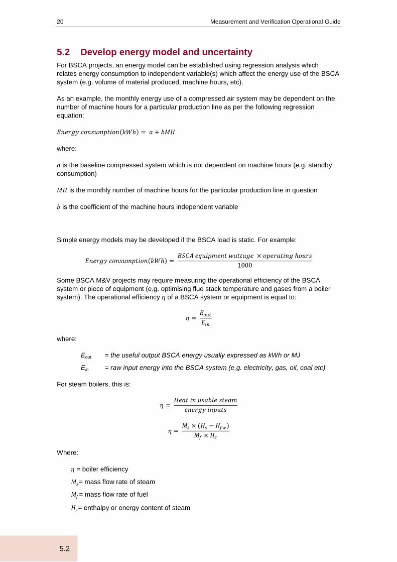
5.2 Develop energy model and uncertainty For BSCA projects, an energy model can be established using regression analysis which relates energy consumption to independent variable(s) which affect the energy use of the BSCA system (e.g. volume of material produced, machine hours, etc).
As an example, the monthly energy use of a compressed air system may be dependent on the number of machine hours for a particular production line as per the following regression equation:
𝐸𝑛𝑒𝑟𝑔𝑦 𝑐𝑜𝑛𝑠𝑢𝑚𝑝𝑡𝑖𝑜𝑛(𝑘𝑊ℎ) = 𝑎 + 𝑏𝑀𝐻
where:
𝑎 is the baseline compressed system which is not dependent on machine hours (e.g. standby consumption)
𝑀𝐻 is the monthly number of machine hours for the particular production line in question
𝑏 is the coefficient of the machine hours independent variable
Simple energy models may be developed if the BSCA load is static. For example:
𝐸𝑛𝑒𝑟𝑔𝑦 𝑐𝑜𝑛𝑠𝑢𝑚𝑝𝑡𝑖𝑜𝑛(𝑘𝑊ℎ) = 𝐵𝑆𝐶𝐴 𝑒𝑞𝑢𝑖𝑝𝑚𝑒𝑛𝑡 𝑤𝑎𝑡𝑡𝑎𝑔𝑒 × 𝑜𝑝𝑒𝑟𝑎𝑡𝑖𝑛𝑔 ℎ𝑜𝑢𝑟𝑠
1000
Some BSCA M&V projects may require measuring the operational efficiency of the BSCA system or piece of equipment (e.g. optimising flue stack temperature and gases from a boiler system). The operational efficiency η of a BSCA system or equipment is equal to:
𝜂 = 𝐸𝑜𝑢𝑡𝐸𝑖𝑛
where:
Eout = the useful output BSCA energy usually expressed as kWh or MJ
Ein = raw input energy into the BSCA system (e.g. electricity, gas, oil, coal etc)
For steam boilers, this is:
𝜂 = 𝐻𝑒𝑎𝑡 𝑖𝑛 𝑢𝑠𝑎𝑏𝑙𝑒 𝑠𝑡𝑒𝑎𝑚
𝑒𝑛𝑒𝑟𝑔𝑦 𝑖𝑛𝑝𝑢𝑡𝑠
𝜂 = 𝑀𝑠 × (𝐻𝑠 − 𝐻𝑓𝑤)
𝑀𝑓 × 𝐻𝑐
Where:
𝜂 = boiler efficiency
𝑀𝑠= mass flow rate of steam
𝑀𝑓= mass flow rate of fuel
𝐻𝑠= enthalpy or energy content of steam

Data collection, modelling and analysis
21
5.3
𝐻𝑓𝑤= enthalpy or energy content of feed water
𝐻𝑐= net heating value of fuel in kJ/kg
The useful output BSCA energy Eout will typically be a fluid flow such as hot water, steam, compressed air and can be calculated by the following equation:
𝐸𝑜𝑢𝑡(𝑀𝐽) = � 𝑉𝜌𝐶𝑝∆𝑇 𝑑𝑡𝑡
0
where:
V = volumetric flow rate of the fluid usually expressed in litres per second L/s
ρ = density of the fluid usually expressed as m3/kg
сp = specific heat capacity of the fluid usually expressed as kJ/kgK
∆T = temperature differential of the flow and return fluid usually expressed as ºC or K
dt = time incremental of the calculation – summing the energy of each time incremental from 0 to t equals the total fluid flow energy during the measurement period.
Other forms of energy models do exist, particularly for steam where energy flows are typically calculated using enthalpy equations and steam tables which is outside the scope of this M&V guide.
Uncertainty can be introduced into the energy model due to inaccuracies of measurement equipment, sampling errors and regression modelling errors. These inaccuracies need to be quantified as an overall uncertainty statement which includes a precision and confidence level. Refer to the Process Guide for further guidance on calculating and expressing uncertainty.
5.3 Implement ECM(s) During the implementation phase of ECM(s), no M&V baseline or post retrofit data should be collected. Measurement and collection of post retrofit data can commence after ECM(s) have been installed and commissioned, preferably allowing for a period of time for the ECM(s) to be “embedded” into normal operations.
5.4 Measure post retrofit data Conduct post-retrofit measurement in line with the prepared M&V plan using the same techniques as for the baseline (section 5.1). Position the measurement equipment in the same place where possible. Ensure appropriate records are kept and take photographs.
Collect any associated data required for calculating post-retrofit energy use or adjustments based on independent variables (e.g. changes in operating hours). Confirm data integrity and completeness.
Post-retrofit performance should not be measured immediately post-retrofit, but allow for a “bedding-in” period prior to measurement.

Measurement and Verification Operational Guide
22
5.5
5.5 Savings analysis and uncertainty The general equation for energy savings is:
Energy Savings = (Baseline Energy – Post-Retrofit Energy) ± Adjustments
In the case of BSCA projects where the power draw and operating hours are relatively static and can easily be measured, energy savings can be calculated as:
kWhsavings = (kWbase x OHbase) – (kWpost x OHpost) ± Adjustments
Where:
kWhsavings = total energy savings, measured in kilowatt-hours (kWh)
kWbase = the kilowatt (kW) demand of the BSCA equipment
kWpost = the kilowatt (kW) demand of the retrofit BSCA equipment
OHbase = operating hours during the baseline period
OHpost = operating hours during the post-retrofit period
Source: San Diego Gas and Electric
For BSCA efficiency projects with static power draws, minimal adjustments and unchanged operating hours, this may be simplified to:
kWh savings = (kWbase – kWpost) x OH
For BSCA control projects with minimal adjustments and unchanged power draw, this may be simplified to:
kWh savings = (OHbase – OHpost) x kW
Whilst for BSCA operational efficiency projects with minimal adjustments and little variability of annual energy consumption of the BSCA system, this may be simplified to:
kWh savings = kWhbase x (ηbase – ηpost)
Where:
kWhbase = total base year energy consumption of the BSCA system/equipment
ηbase = operational BSCA efficiency during the baseline period
ηpost = operational BSCA efficiency during the post-retrofit period
BSCA efficiency projects can result in reduced demand. Demand savings are calculated as follows:
kW savings = (Baseline demand – Post-retrofit demand) ± Adjustments
For BSCA efficiency projects, this may be simplified to:
kW savings = kWbase – kWpost
Cost savings are determined by multiplying the energy and demand savings by the appropriate cost rates.

Data collection, modelling and analysis
23
5.5
Annual Cost Savings ($) = Demand Saving + Energy Saving
= ([kW savings] x [monthly demand cost rate] x 12)
+ ([kWh savings] x [energy cost rate])
5.5.1 Extrapolation If a sample-based approach is used (selected BSCA systems and/or sites), then extrapolate across the project’s measurement boundary or across the population.
Extrapolate the calculated savings for the measured period as required.
5.5.2 Uncertainty Estimate the savings uncertainty, based on the measurement approach, placement, impact of variables, length of measurement and equipment used. Refer to the Process Guide for further guidance on calculating and expressing uncertainty.

Measurement and Verification Operational Guide
24
6.1
6 Finish
6.1 Reporting Prepare an outcomes report summarising the M&V exercise. Ensure any extrapolated savings are referred to as estimates, as the ‘actual’ savings only apply to the measurement period. Energy uncertainty is expressed with the overall precision and confidence level.
6.2 Project close and savings persistence Periodic performance review of the retrofit may also be undertaken to confirm ongoing savings. This may not require the measurement of power usage but may be limited to: § An inspection of the area to ensure equipment remains consistent with that specified in the
installation § Review of operational patterns and control set points. § Wear and tear of BSCA equipment and reduction in operational efficiency.
M&V Examples
25
7.1
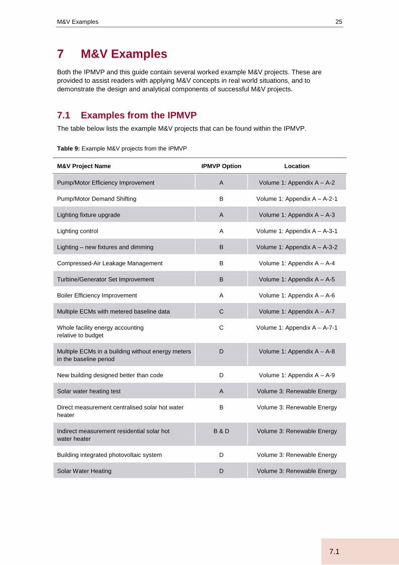
7 M&V Examples Both the IPMVP and this guide contain several worked example M&V projects. These are provided to assist readers with applying M&V concepts in real world situations, and to demonstrate the design and analytical components of successful M&V projects.
7.1 Examples from the IPMVP The table below lists the example M&V projects that can be found within the IPMVP.
Table 9: Example M&V projects from the IPMVP
M&V Project Name IPMVP Option Location
Pump/Motor Efficiency Improvement A Volume 1: Appendix A – A-2
Pump/Motor Demand Shifting B Volume 1: Appendix A – A-2-1
Lighting fixture upgrade A Volume 1: Appendix A – A-3
Lighting control A Volume 1: Appendix A – A-3-1
Lighting – new fixtures and dimming B Volume 1: Appendix A – A-3-2
Compressed-Air Leakage Management B Volume 1: Appendix A – A-4
Turbine/Generator Set Improvement B Volume 1: Appendix A – A-5
Boiler Efficiency Improvement A Volume 1: Appendix A – A-6
Multiple ECMs with metered baseline data C Volume 1: Appendix A – A-7
Whole facility energy accounting relative to budget
C Volume 1: Appendix A – A-7-1
Multiple ECMs in a building without energy meters in the baseline period
D Volume 1: Appendix A – A-8
New building designed better than code D Volume 1: Appendix A – A-9
Solar water heating test A Volume 3: Renewable Energy
Direct measurement centralised solar hot water heater
B Volume 3: Renewable Energy
Indirect measurement residential solar hot water heater
B & D Volume 3: Renewable Energy
Building integrated photovoltaic system D Volume 3: Renewable Energy
Solar Water Heating D Volume 3: Renewable Energy

Measurement and Verification Operational Guide
26
7.2
7.2 Examples from this guide The table below lists the example M&V projects that can be found within this guide.
Table 10: Example M&V projects from the M&V Operational Guide
M&V Project Name IPMVP Option Location
M&V design examples A, B, C, D Process: Appendix A
Demand and cost avoidance calculation example n/a Process: Appendix A
Regression modelling and validity testing n/a Process: Appendix E
Lighting fixture replacement within an office tenancy A Applications: Lighting – Scenario A
Lighting fixture and control upgrade at a function centre A Applications: Lighting – Scenario B
Lighting fixture retrofit incorporating daylight control B Applications: Lighting – Scenario C
Pump retrofit and motor replacement A Applications: Motors, Pumps and Fans –
Scenario A
Car park ventilation involving CO monitoring and variable speed drive on fans
B Applications: Motors, Pumps and Fans – Scenario B
Replacement an inefficient gas boiler with a high efficiency one C Applications: Heating, Ventilation and
Cooling – Scenario A
Upgrade freezer controls within a food processing plant B Applications: Commercial and Industrial
Refrigeration – Scenario A
Compressed air leak detection within a manufacturing site using sampling analysis
B Applications: Boilers, Steam and Compressed Air – Scenario A
Steam system leak detection within a food processing site using regression analysis
B Applications: Boilers, Steam and Compressed Air – Scenario B
Multiple ECMs involving compressed air and steam system optimisation, combined with lighting controls at a cannery
C Applications: Whole Buildings – Scenario A
Commercial building air conditioning central plant upgrade C Applications: Whole Buildings –
Scenario B
Evaluate performance efficiency of a newly installed cogeneration unit a a school
D Applications: Renewables and Cogeneration – Scenario A
Installation of a cogeneration plant at a hospital C Applications: Renewables and
Cogeneration – Scenario B
Use of solar hot water system on a housing estate B Applications: Renewables and
Cogeneration – Scenario C
Appendix A: Example scenario A
27
Appendix A
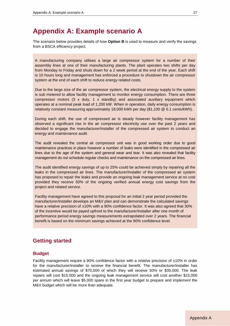
Appendix A: Example scenario A The scenario below provides details of how Option B is used to measure and verify the savings from a BSCA efficiency project.
A manufacturing company utilises a large air compressor system for a number of their assembly lines at one of their manufacturing plants. The plant operates two shifts per day from Monday to Friday and shuts down for a 2 week period at the end of the year. Each shift is 10 hours long and management has enforced a procedure to shutdown the air compressor system at the end of each shift to reduce energy related costs.
Due to the large size of the air compressor system, the electrical energy supply to the system is sub metered to allow facility management to monitor energy consumption. There are three compressor motors (3 x duty, 1 x standby) and associated auxiliary equipment which operates at a nominal peak load of 1,200 kW. When in operation, daily energy consumption is relatively constant measuring approximately 18,000 kWh per day ($1,100 @ 6.1 cents/kWh).
During each shift, the use of compressed air is steady however facility management has observed a significant rise in the air compressor electricity use over the past 2 years and decided to engage the manufacturer/installer of the compressed air system to conduct an energy and maintenance audit.
The audit revealed the central air compressor unit was in good working order due to good maintenance practices in place however a number of leaks were identified in the compressed air lines due to the age of the system and general wear and tear. It was also revealed that facility management do not schedule regular checks and maintenance on the compressed air lines.
The audit identified energy savings of up to 25% could be achieved simply by repairing all the leaks in the compressed air lines. The manufacturer/installer of the compressed air system has proposed to repair the leaks and provide an ongoing leak management service at no cost provided they receive 50% of the ongoing verified annual energy cost savings from the project and related service.
Facility management have agreed to this proposal for an initial 2 year period provided the manufacturer/installer develops an M&V plan and can demonstrate the calculated savings have a relative precision of ±10% with a 90% confidence factor. It was also agreed that 30% of the incentive would be payed upfront to the manufacturer/installer after one month of performance period energy savings measurements extrapolated over 2 years. The financial benefit is based on the minimum savings achieved at the 90% confidence level.
Getting started
Budget Facility management require a 90% confidence factor with a relative precision of ±10% in order for the manufacturer/installer to receive the financial benefit. The manufacturer/installer has estimated annual savings of $70,000 of which they will receive 50% or $35,000. The leak repairs will cost $15,000 and the ongoing leak management service will cost another $15,000 per annum which will leave $5,000 spare in the first year budget to prepare and implement the M&V budget which will be more than adequate.
Measurement and Verification Operational Guide
28
Appendix A
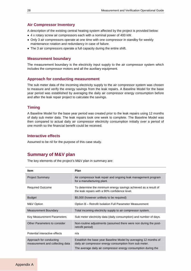
Air Compressor Inventory A description of the existing central heating system affected by the project is provided below: § 4 x rotary screw air compressors each with a nominal power of 400 kW. § Only 3 air compressors operate at one time with one compressor in standby for weekly
maintenance rotation and redundancy in case of failure. § The 3 air compressors operate a full capacity during the entire shift.
Measurement boundary The measurement boundary is the electricity input supply to the air compressor system which includes the compressor motors and all the auxiliary equipment.
Approach for conducting measurement The sub meter data of the incoming electricity supply to the air compressor system was chosen to measure and verify the energy savings from the leak repairs. A Baseline Model for the base year period was established by averaging the daily air compressor energy consumption before and after the leak repair project to calculate the savings.
Timing A Baseline Model for the base year period was created prior to the leak repairs using 12 months of daily sub meter data. The leak repairs took one week to complete. The Baseline Model was then compared to actual daily air compressor electricity consumption initially over a period of one month so the financial benefit could be received.
Interactive effects Assumed to be nil for the purpose of this case study.
Summary of M&V plan The key elements of the project’s M&V plan in summary are:
Item Plan
Project Summary Air compressor leak repair and ongoing leak management program for a manufacturing plant.
Required Outcome To determine the minimum energy savings achieved as a result of the leak repairs with a 90% confidence level.
Budget $5,000 (however unlikely to be required)
M&V Option Option B – Retrofit Isolation Full Parameter Measurement
Measurement Boundary Total incoming electricity supply to air compressor system.
Key Measurement Parameters Sub meter electricity data (daily consumption) and number of days.
Other Parameters to consider Non-routine adjustments (assumed there were non during the post-retrofit period)
Potential interactive effects n/a
Approach for conducting measurement and collecting data
Establish the base year Baseline Model by averaging 12 months of daily air compressor energy consumption from sub meter. The average daily air compressor energy consumption during the
Appendix A: Example scenario A
29
Appendix A
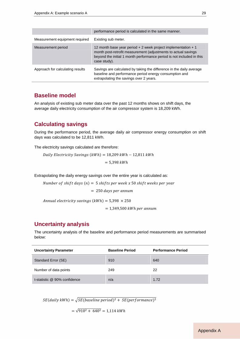
performance period is calculated in the same manner.
Measurement equipment required Existing sub meter.
Measurement period 12 month base year period + 2 week project implementation + 1 month post-retrofit measurement (adjustments to actual savings beyond the initial 1 month performance period is not included in this case study).
Approach for calculating results Savings are calculated by taking the difference in the daily average baseline and performance period energy consumption and extrapolating the savings over 2 years.
Baseline model An analysis of existing sub meter data over the past 12 months shows on shift days, the average daily electricity consumption of the air compressor system is 18,209 kWh.
Calculating savings During the performance period, the average daily air compressor energy consumption on shift days was calculated to be 12,811 kWh.
The electricity savings calculated are therefore:
𝐷𝑎𝑖𝑙𝑦 𝐸𝑙𝑒𝑐𝑡𝑟𝑖𝑐𝑖𝑡𝑦 𝑆𝑎𝑣𝑖𝑛𝑔𝑠 (𝑘𝑊ℎ) = 18,209 𝑘𝑊ℎ − 12,811 𝑘𝑊ℎ
= 5,398 𝑘𝑊ℎ
Extrapolating the daily energy savings over the entire year is calculated as:
𝑁𝑢𝑚𝑏𝑒𝑟 𝑜𝑓 𝑠ℎ𝑖𝑓𝑡 𝑑𝑎𝑦𝑠 (𝑛) = 5 𝑠ℎ𝑖𝑓𝑡𝑠 𝑝𝑒𝑟 𝑤𝑒𝑒𝑘 𝑥 50 𝑠ℎ𝑖𝑓𝑡 𝑤𝑒𝑒𝑘𝑠 𝑝𝑒𝑟 𝑦𝑒𝑎𝑟
= 250 𝑑𝑎𝑦𝑠 𝑝𝑒𝑟 𝑎𝑛𝑛𝑢𝑚
𝐴𝑛𝑛𝑢𝑎𝑙 𝑒𝑙𝑒𝑐𝑡𝑟𝑖𝑐𝑖𝑡𝑦 𝑠𝑎𝑣𝑖𝑛𝑔𝑠 (𝑘𝑊ℎ) = 5,398 × 250
= 1,349,500 𝑘𝑊ℎ 𝑝𝑒𝑟 𝑎𝑛𝑛𝑢𝑚
Uncertainty analysis The uncertainty analysis of the baseline and performance period measurements are summarised below:
Uncertainty Parameter Baseline Period Performance Period
Standard Error (SE) 910 640
Number of data points 249 22
t-statistic @ 90% confidence n/a 1.72
𝑆𝐸(𝑑𝑎𝑖𝑙𝑦 𝑘𝑊ℎ) = �𝑆𝐸(𝑏𝑎𝑠𝑒𝑙𝑖𝑛𝑒 𝑝𝑒𝑟𝑖𝑜𝑑)2 + 𝑆𝐸(𝑝𝑒𝑟𝑓𝑜𝑟𝑚𝑎𝑛𝑐𝑒)2
= √9102 + 6402 = 1,114 𝑘𝑊ℎ
Measurement and Verification Operational Guide
30
Appendix A
Extrapolating the SE across the entire year results in:
𝑆𝐸(𝑎𝑛𝑛𝑢𝑎𝑙 𝑠𝑎𝑣𝑖𝑛𝑔𝑠) = �250𝑥 1,1142 = 17,602 𝑘𝑊ℎ
Using a t-statistic of 1.72 (22 measurement points with 90% confidence), the range of possible annual savings will be:
𝑅𝑎𝑛𝑔𝑒 𝑜𝑓 𝑆𝑎𝑣𝑖𝑛𝑔𝑠 (𝑘𝑊ℎ) = 1,349,500 ± 1.72 × 17,602 𝑘𝑊ℎ
= 1,349,500 ± 30,275 𝑘𝑊ℎ
= 1,319,225 𝑡𝑜 1,379,775 𝑘𝑊ℎ
The relative precision of the annual savings reported is thus 2.3% (100 x 30,275 / 1,349,500)
Reporting results The savings results can be described by the following:
The one month post-retrofit annual savings extrapolated for an entire year is calculated to be 1,349,500 kWh ±2.3% with a 90% confidence factor. The relative precision is within the required agreed range of ±10%. In other words, one can be 90% confident that the electricity savings achieved during the one month post-retrofit period ranged between 1,319,226 to 1,379,774 kWh ($80,472 to $84,166 @ 6.1 cents/kWh).
The manufacturer/installer will therefore by entitled to an upfront financial benefit equalling 30% of half the verified minimum range savings at the 90% confidence level extrapolated over the 2 year period. This will total to $24,141.
Appendix B: Example scenario B
31
Appendix B
Appendix B: Example scenario B The scenario below provides details of how Option B is used to measure and verify the savings from a Steam system leak detection program.
A local producer of packaged foods operates a major food processing plant in Newcastle. The plant produces two major lines; chips and cereals. Both processes involve the use of steam for sterilisation and cooking.
The site uses 10 bar saturated steam, which is supplied by two 4MW boilers and a 2MW boiler, which all operate on natural gas. Over the last 12 months, the boilers have consumed 88,500 GJ of natural gas at a cost of almost $465,000. The site also uses an extensive amount of natural gas within ovens and for drying.
Recent increase in energy prices has prompted the site’s operations manager to look at ways to reduce costs. In addition to other systems, the manager has focused on the site’s steam system. Most components of this system are around 16 years old however the site did replace the boiler about 3 years ago.
The steam system was audited as part of an ‘Energy Saver’ audit – co-funded by the state government - and it was found that the distribution lines must be suffering from steam leaks, as the amount of steam being generated was considerably higher than estimated load requirements.
A leak detection and elimination program has been scheduled for implementation. As a sponsor of the audit, the state government is seeking formal measurement and verification of the system savings. The government is seeking verification to 95% confidence.
Getting started
Budget The site has existing sub metering in place to measure the input natural gas feeding the boiler plant room, as well as a meters and sensors at the main distribution line measuring the steam temperature, pressure and flow. Energy consumption, steam use and corresponding production data for the Chips and Cereals product lines is all captured and stored within the site’s SCADA system.
As a result, the site has access to a full 12 months of baseline data and so for this reason an Option B approach will be used.
The M&V project will be conducted by the operations manager. A nominal budget of $2,000 has been allocated.
Measurement Boundary The measurement boundary is site’s steam system, which includes the boiler plant room, and steam distribution lines. Data will be measured using existing meters as recorded within the site’s SCADA system.
Measurement and Verification Operational Guide
32
Appendix B
Approach for Conducting Measurement This ECM involves making improvements to the steam distribution system (by eliminating leaks). The effects of this ECM are: § The amount of steam required to produce tonnes of Chips and Cereals should reduce, due to
the elimination of steam being lost due to leaks. § Boiler efficiency should not be affected, although with a reduction in the amount of steam
required, boilers may operate at part load, or staging may be affected.
Given these two effects, we are seeking to relate either generated steam or input natural gas to production output, so that we can capture the efficiency improvement in kilograms of steam per tonne of product, or better yet, input megajoules per tonne of product.
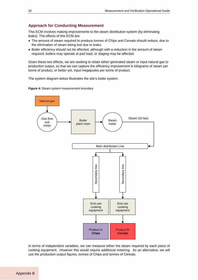
The system diagram below illustrates the site’s boiler system.
Figure 4: Steam system measurement boundary
In terms of independent variables, we can measure either the steam required by each piece of cooking equipment. However this would require additional metering. As an alternative, we will use the production output figures, tonnes of Chips and tonnes of Cereals.
Boiler plant room
Natural gas
Gas flow sub
meter
Steam meter
Steam (10 bar)
Sec
onda
ry li
ne
Main distribution Line
Sec
onda
ry li
ne
End use cooking
equipment
Product A: Chips
Product B: Cereals
End use cooking
equipment
Appendix B: Example scenario B
33
Appendix B
In terms of evaluating the change in system efficiency, we could measure either steam or natural gas at the meters shown above.
In this case, we cannot use the steam meter as representing the independent variable for the system load requirement. This is because the relationship between steam use and the amount of production will change, and hence we need to capture what is required (either steam at the equipment level or production output) rather than what is initially supplied to the distribution system.
Due to the presence of the input natural gas meter, it has been decided to evaluate input natural gas against production figures for Chips and Cereals.
The sub meter data will be downloaded from the SCADA system. Other key parameters will be production figures for Chips and Cereals.
A Baseline Model for the base year period will be established by performing a regression analysis on Chips (tonnes) and Cereals (tonnes). The Baseline Model will then be ‘adjusted’ to forecast the ‘business as usual’ natural gas consumption across the post-retrofit period, by applying the relevant data for Chips (tonnes) and Cereals (tonnes) to the model.
The difference between the Adjusted Baseline Energy and the measured Post-Retrofit energy use will be calculated to determine the energy savings.
Timing The ECM was implemented in August 2011. A Baseline Model for the base year period will be created prior for the 12 month period immediately preceding the upgrade. The post-retrofit period will consist of the months following the upgrade to the current month, namely July 2010 to June 2011.
Interactive effects The measurement boundary comprises the entire central plant, and as such includes components that may cause interactive effects. Waste heat is recovered from the boilers however this is used to pre-heat the feedwater. As a result, it is determined that there are no significant interactive effects.
Summary of M&V Plan The key elements of the project’s M&V plan in summary are:
Item Plan
Project Summary Steam leak detection and elimination program to occur on main and secondary distribution lines
Required Outcome To prepare a robust M&V outcome for submission to state government a minimum 95% confidence level.
Budget $4,000
M&V Option Option B – Full parameter measurement
Measurement Boundary The site’s entire steam system including central boiler plant, main and secondary distribution lines and end use equipment.

Measurement and Verification Operational Guide
34
Appendix B
Item Plan
Key Measurement Parameters
Sub meter natural gas data (daily data) production data for Chips and Cereals (monthly data).
Other Parameters to consider
Non-routine adjustments (assumed there were none during the post-retrofit period)
Potential interactive effects None identified
Approach for conducting measurement and collecting data
Established the base year Baseline Model via regression analysis using monthly natural gas sub meter data and monthly data for production of Chips and Cereals. Monthly data collected via SCADA from natural gas sub meter.
Measurement equipment required
Existing natural gas sub meter will be used.
Measurement period 12 month base year period + 1 month project implementation + 3 month post retrofit operation without measurement + 12 months post-retrofit measurement.
Approach for calculating results
Savings are calculated by entering the monthly data for Chips and Cereals production into the Baseline Model during the post-retrofit period and calculating the difference against actual monthly metered data consumption to determine the energy savings. Cost savings will be calculated using an average rate = $05.26/GJ Greenhouse gas emissions reduction will be calculated using a greenhouse gas coefficient = 51.33 kg CO2-e/GJ
Baseline model The chart below plots the monthly baseline natural gas usage against production figures for Chips and Cereals.
An initial regression analysis was conducted using combined ‘total production’ figures. Although this resulted in a fairly strong relationship, a multi-variable analysis was also performed.
0
500
1,000
1,500
2,000
2,500
3,000
3,500
4,000
4,500
-
3,000
6,000
9,000
Jul-1
0
Aug-
10
Sep-
10
Oct
-10
Nov-
10
Dec-
10
Jan-
11
Feb-
11
Mar
-11
Apr-
11
May
-11
Jun-
11
Prod
uctio
n (T
onne
s)
Nat
ural
Gas
(GJ)
Natural Gas (GJ)
Chips
Cereals
Appendix B: Example scenario B
35
Appendix B
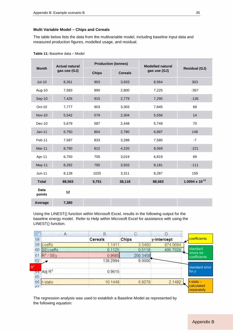
Multi Variable Model – Chips and Cereals
The table below lists the data from the multivariable model, including baseline input data and measured production figures, modelled usage, and residual.
Table 11: Baseline data – Model
Month Actual natural gas use (GJ)
Production (tonnes) Modelled natural
gas use (GJ) Residual (GJ) Chips Cereals
Jul-10 8,261 903 3,933 8,564 303
Aug-10 7,583 890 2,800 7,225 -357
Sep-10 7,426 915 2,779 7,290 -136
Oct-10 7,777 903 3,303 7,845 68
Nov-10 5,542 579 2,304 5,556 14
Dec-10 5,679 587 2,448 5,749 70
Jan-11 6,750 804 2,780 6,897 148
Feb-11 7,587 833 3,288 7,580 -7
Mar-11 8,790 812 4,220 8,569 -221
Apr-11 6,750 705 3,019 6,819 69
May-11 8,292 795 3,933 8,181 -111
Jun-11 8,128 1025 3,311 8,287 159
Total 88,563 9,751 38,118 88,563 1.0004 x 10⁻¹¹
Data points 12
Average 7,380
Using the LINEST() function within Microsoft Excel, results in the following output for the baseline energy model. Refer to Help within Microsoft Excel for assistance with using the LINEST() function.
The regression analysis was used to establish a Baseline Model as represented by the following equation:
standard errors for coefficients
coefficients
standard error for y
R2
t-stats – calculated separately

Measurement and Verification Operational Guide
36
Appendix B
𝑀𝑜𝑛𝑡ℎ𝑙𝑦 𝑛𝑎𝑡𝑢𝑟𝑎𝑙 𝑔𝑎𝑠 𝑢𝑠𝑒 (𝐺𝐽)= 874.0694 + 3.5460 × 𝐶ℎ𝑖𝑝𝑠(𝑡𝑜𝑛𝑛𝑒𝑠) + 1.1411 × 𝐶𝑒𝑟𝑒𝑎𝑙𝑠(𝑡𝑜𝑛𝑛𝑒𝑠)
The R2 value is 0.9685 and the standard error is 200.3458 GJ
Statistical validation of the baseline model The baseline model was validated to confirm that it can be used. This involves equating some additional attributes and confirming its validity. The attributes to be reviewed are:
Attribute Description and Validity Test Model 1
R2
Must be 0.75 or higher. Output from LINEST() function
R2 = 0.9685
t-statistic for each coefficient
Determine the validity of each x coefficient. Values must be greater than 2. Each ‘t-stat’ is calculated as follows:
𝑡𝑋𝑛 =𝑐𝑜𝑒𝑓𝑓𝑖𝑐𝑖𝑒𝑛𝑡𝑋𝑛
𝑠𝑡𝑎𝑛𝑑𝑎𝑟𝑑 𝑒𝑟𝑟𝑜𝑟𝑋𝑛
t-stats for Chips and Cereals coefficients are:
𝑡𝑐ℎ𝑖𝑝𝑠 =3.54600.5118
= 6.9278
𝑡𝑐𝑒𝑟𝑒𝑎𝑙𝑠 =1.14110.1125
= 10.1449
Absolute mean bias (MBE)
Determines the overall bias in the regression estimate. MBE values should be < 0.005%. Calculated as follows:
𝑀𝐵𝐸 =∑(𝑚𝑜𝑑𝑒𝑙𝑙𝑒𝑑𝑛 − 𝑎𝑐𝑡𝑢𝑎𝑙𝑛)
𝑛
Where: n = the number of samples modelledn = predicted value for sample item n actualn = actual value for sample item n
Applying the model to each set of monthly production values, and subtracting the actual reading from the month, the resulting ‘residual’ is 1.0004x10⁻¹¹.
𝑀𝐵𝐸 =1.0004 × 10⁻¹¹
12
= 8.34 × 10⁻¹³
Monthly Mean Error CV(RMSE)
Related to the standard error of the model. CV(RMSE) values should be < 0.25. Calculated as follows:
𝐶𝑉(𝑅𝑀𝑆𝐸) =𝑠𝑡𝑎𝑛𝑑𝑎𝑟𝑑 𝑒𝑟𝑟𝑜𝑟 𝑓𝑜𝑟 𝑦𝑎𝑣𝑒𝑟𝑎𝑔𝑒(𝑎𝑐𝑡𝑢𝑎𝑙 𝑣𝑎𝑙𝑢𝑒𝑠)
𝐶𝑉(𝑅𝑀𝑆𝐸) =200.357,380
= 0.0271
The model has passed all of the statistical validity tests above, thus both models below could potentially be used.
The baseline model is:
𝑀𝑜𝑛𝑡ℎ𝑙𝑦 𝑛𝑎𝑡𝑢𝑟𝑎𝑙 𝑔𝑎𝑠 𝑢𝑠𝑒 (𝐺𝐽)= 874.0694 + 3.5460 × 𝐶ℎ𝑖𝑝𝑠(𝑡𝑜𝑛𝑛𝑒𝑠) + 1.1411 × 𝐶𝑒𝑟𝑒𝑎𝑙𝑠(𝑡𝑜𝑛𝑛𝑒𝑠)
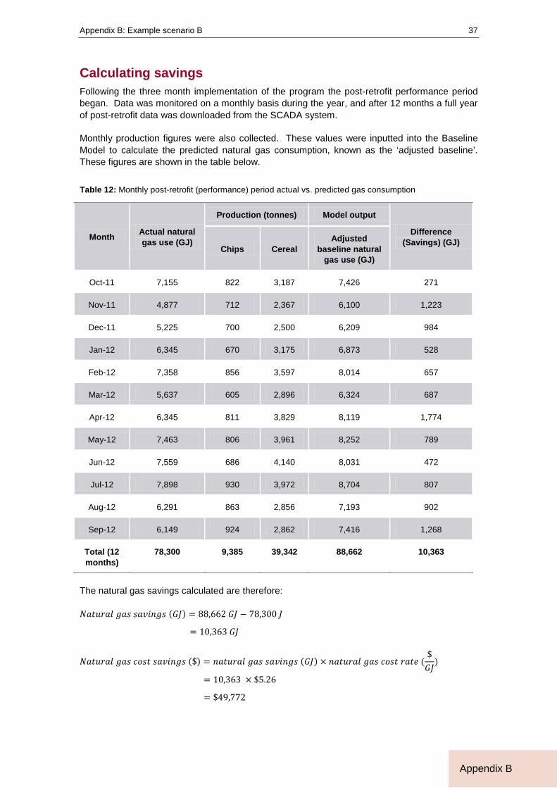
Appendix B: Example scenario B
37
Appendix B
Calculating savings Following the three month implementation of the program the post-retrofit performance period began. Data was monitored on a monthly basis during the year, and after 12 months a full year of post-retrofit data was downloaded from the SCADA system.
Monthly production figures were also collected. These values were inputted into the Baseline Model to calculate the predicted natural gas consumption, known as the ‘adjusted baseline’. These figures are shown in the table below.
Table 12: Monthly post-retrofit (performance) period actual vs. predicted gas consumption
Month Actual natural gas use (GJ)
Production (tonnes) Model output
Difference (Savings) (GJ)
Chips Cereal Adjusted
baseline natural gas use (GJ)
Oct-11 7,155 822 3,187 7,426 271
Nov-11 4,877 712 2,367 6,100 1,223
Dec-11 5,225 700 2,500 6,209 984
Jan-12 6,345 670 3,175 6,873 528
Feb-12 7,358 856 3,597 8,014 657
Mar-12 5,637 605 2,896 6,324 687
Apr-12 6,345 811 3,829 8,119 1,774
May-12 7,463 806 3,961 8,252 789
Jun-12 7,559 686 4,140 8,031 472
Jul-12 7,898 930 3,972 8,704 807
Aug-12 6,291 863 2,856 7,193 902
Sep-12 6,149 924 2,862 7,416 1,268
Total (12 months)
78,300 9,385 39,342 88,662 10,363
The natural gas savings calculated are therefore:
𝑁𝑎𝑡𝑢𝑟𝑎𝑙 𝑔𝑎𝑠 𝑠𝑎𝑣𝑖𝑛𝑔𝑠 (𝐺𝐽) = 88,662 𝐺𝐽 − 78,300 𝐽
= 10,363 𝐺𝐽
𝑁𝑎𝑡𝑢𝑟𝑎𝑙 𝑔𝑎𝑠 𝑐𝑜𝑠𝑡 𝑠𝑎𝑣𝑖𝑛𝑔𝑠 ($) = 𝑛𝑎𝑡𝑢𝑟𝑎𝑙 𝑔𝑎𝑠 𝑠𝑎𝑣𝑖𝑛𝑔𝑠 (𝐺𝐽) × 𝑛𝑎𝑡𝑢𝑟𝑎𝑙 𝑔𝑎𝑠 𝑐𝑜𝑠𝑡 𝑟𝑎𝑡𝑒 ($𝐺𝐽
)
= 10,363 × $5.26
= $49,772

Measurement and Verification Operational Guide
38
Appendix B
𝐺𝑟𝑒𝑒𝑛ℎ𝑜𝑢𝑠𝑒 𝑔𝑎𝑠 𝑒𝑚𝑖𝑠𝑠𝑖𝑜𝑛 𝑟𝑒𝑑𝑢𝑐𝑡𝑖𝑜𝑛 (𝑡.𝐶𝑂2𝑒)
= 𝑛𝑎𝑡𝑢𝑟𝑎𝑙 𝑔𝑎𝑠 𝑠𝑎𝑣𝑖𝑛𝑔𝑠 (𝐺𝐽) × 𝑔𝑟𝑒𝑒𝑛ℎ𝑜𝑢𝑠𝑒 𝑔𝑎𝑠 𝑐𝑜𝑒𝑓𝑓𝑖𝑐𝑖𝑒𝑛𝑡 (𝑘𝐺.𝐶𝑂2𝑒) ×1
1000
= 10,363 × 51.33 ×1
1000
= 531.9 𝑡.𝐶𝑂2𝑒
A graphical representation of the base year period vs. performance period actual and calculated predicted natural gas consumption is presented in the figure below.
It can be seen that during the baseline period (and prior), the model predicts the monthly natural gas use highly accurately.
Uncertainty Analysis The standard error of the regression model was calculated to be 200.3458, as shown in the LINEST() output. This is equivalent to applying the following equation to the baseline dataset:
𝑆𝐸𝑌� = �∑�𝑌�𝑖 − 𝑌𝑖�
2
𝑛 − 𝑝 − 1
Where:
𝑌�𝑖 𝑖𝑠 𝑡ℎ𝑒 𝑝𝑟𝑒𝑑𝑖𝑐𝑡𝑒𝑑 𝑣𝑎𝑙𝑢𝑒 𝑜𝑓 𝑒𝑛𝑒𝑟𝑔𝑦 (𝑌)𝑓𝑟𝑜𝑚 𝑡ℎ𝑒 𝑟𝑒𝑔𝑟𝑒𝑠𝑠𝑖𝑜𝑛 𝑚𝑜𝑑𝑒𝑙
𝑌𝑖 𝑖𝑠 𝑡ℎ𝑒 𝑎𝑐𝑡𝑢𝑎𝑙 𝑜𝑏𝑠𝑒𝑟𝑣𝑒𝑑 𝑣𝑎𝑙𝑢𝑒 𝑜𝑓 𝑒𝑛𝑒𝑟𝑔𝑦 𝑓𝑟𝑜𝑚 𝑡ℎ𝑒 𝑔𝑎𝑠 𝑖𝑛𝑣𝑜𝑖𝑐𝑒
𝑛 𝑖𝑠 𝑡ℎ𝑒 𝑛𝑢𝑚𝑏𝑒𝑟 𝑜𝑓 𝑜𝑏𝑠𝑒𝑟𝑣𝑎𝑡𝑖𝑜𝑛𝑠 (𝑛 = 12)
𝑝 𝑖𝑠 𝑡ℎ𝑒 𝑛𝑢𝑚𝑏𝑒𝑟 𝑜𝑓 𝑖𝑛𝑑𝑒𝑝𝑒𝑛𝑑𝑒𝑛𝑡 𝑣𝑎𝑟𝑖𝑎𝑏𝑙𝑒𝑠 𝑖𝑛 𝑡ℎ𝑒 𝑟𝑒𝑔𝑟𝑒𝑠𝑠𝑖𝑜𝑛 𝑒𝑞𝑢𝑎𝑡𝑖𝑜𝑛 (𝑝 = 1)
0
2,000
4,000
6,000
8,000
10,000
12,000
Jul-1
0
Aug-
10
Sep-
10
Oct
-10
Nov-
10
Dec-
10
Jan-
11
Feb-
11
Mar
-11
Apr-
11
May
-11
Jun-
11
Jul-1
1
Aug-
11
Sep-
11
Oct
-11
Nov-
11
Dec-
11
Jan-
12
Feb-
12
Mar
-12
Apr-
12
May
-12
Jun-
12
Jul-1
2
Aug-
12
Sep-
12
Mon
thly
EN
atur
al G
as U
se (G
J)
Natural Gas (GJ) Modelled Gas (GJ)Savings Period:10,363 GJ$49,772532 t.CO2-e11.7%Baseline Period

Appendix B: Example scenario B
39
Appendix B
Using the standard error we can calculate the absolute precision (AP) by applying the t-statistic for our chosen sample size (where DF = 12 data points – 2 variables - 1 = 9) and required confidence (95%). From this table we obtain the t-statistic = 2.26. Refer to Table 27 within Appendix G of the Process Guide for the list of t-statistics.
Absolute precision is calculated as follows:
𝐴𝑏𝑠𝑜𝑙𝑢𝑡𝑒 𝑝𝑟𝑒𝑐𝑖𝑠𝑖𝑜𝑛 (𝐴𝑃) = 𝑡 × 𝑆𝐸
𝐴𝑏𝑠𝑜𝑙𝑢𝑡𝑒 𝑝𝑟𝑒𝑐𝑖𝑠𝑖𝑜𝑛 (𝐴𝑃) = 2.26 × 200.3458 = 452.78 𝐺𝐽
And the relative precision (RP) is calculated by dividing the absolute precision by the average predicted energy use as follows:
𝑟𝑒𝑙𝑎𝑡𝑖𝑣𝑒 𝑝𝑟𝑒𝑐𝑖𝑠𝑖𝑜𝑛 (𝑅𝑃) =𝐴𝑃
𝑎𝑣𝑒𝑟𝑎𝑔𝑒 𝑚𝑜𝑛𝑡ℎ𝑙𝑦 𝑚𝑜𝑑𝑒𝑙𝑙𝑒𝑑 𝑢𝑠𝑎𝑔𝑒
𝑟𝑒𝑙𝑎𝑡𝑖𝑣𝑒 𝑝𝑟𝑒𝑐𝑖𝑠𝑖𝑜𝑛 (𝑅𝑃) =452.78
7,380.29= ±6.1%
For the purposes of this example, errors associated with the sub-meters have been ignored. As such the measured natural gas usage is treated as 100% accurate (SE = 0%). The SE of the monthly savings number will be:
𝑆𝐸(𝑚𝑜𝑛𝑡ℎ𝑙𝑦 𝑠𝑎𝑣𝑖𝑛𝑔𝑠) = �𝑆𝐸(𝑎𝑑𝑗𝑢𝑠𝑡𝑒𝑑 𝑏𝑎𝑠𝑒𝑙𝑖𝑛𝑒)2 + 𝑆𝐸(𝑟𝑒𝑝𝑜𝑟𝑡𝑖𝑛𝑔 𝑝𝑒𝑟𝑖𝑜𝑑 𝑐𝑜𝑛𝑠𝑢𝑚𝑝𝑡𝑖𝑜𝑛)2
= √200.34582 + 02 = 200.3458
Assuming that the standard error for each month’s savings will be the same, the reported savings across 12 months will then have a standard error of:
𝑆𝐸(12 𝑚𝑜𝑛𝑡ℎ 𝑠𝑎𝑣𝑖𝑛𝑔𝑠) = �12 × 200.34582 = 694.02 𝐺𝐽
Using the t-statistic from our baseline model = 2.26 (12 measurement points with 95% confidence, DF = 9), the absolute precision, or range of possible savings across the 12 months will be:
𝐴𝑃 = 2.26 × 694.02 𝐺𝐽
= ±1,568 .5 𝐺𝐽
The relative precision of the 12 months savings reported is thus:
𝑟𝑒𝑙𝑎𝑡𝑖𝑣𝑒 𝑝𝑟𝑒𝑐𝑖𝑠𝑖𝑜𝑛 (𝑅𝑃) =1,568.510,363
= ±15.1%
The range of our savings is:
𝑅𝑎𝑛𝑔𝑒 𝑜𝑓 𝑆𝑎𝑣𝑖𝑛𝑔𝑠 (𝐺𝐽) = 10,363 ± 1,568.5 𝐺𝐽
or
𝑅𝑎𝑛𝑔𝑒 𝑜𝑓 𝑆𝑎𝑣𝑖𝑛𝑔𝑠 (𝐺𝐽) = 10,363 𝐺𝐽 ± 15.1%

Measurement and Verification Operational Guide
40
Appendix B
Reporting results The savings results can be described by the following:
The 12-month post-retrofit savings is calculated to be 10,363 GJ ±15.1% with a 95% confidence factor. Cost savings are $49,772 and the greenhouse gas reduction is 532 t.CO2-e. The savings represent an 11.7% reduction in natural gas use across the measurement boundary.
It can be seen through this example that although we have a somewhat complex system, we have defined a measurement boundary based on the nature of the ECM and available metering and have simply analysed the overall change in input energy use against production output. We were not required to conduct detailed analysis of the boiler itself or the distribution lines – we simply analysed the net result.
For other types of projects, a smaller measurement boundary may be chosen, which may require data collection and analysis of the input energy use versus steam production.