measurement of agricultural income of counties - the national bureau of economic research ·...

This PDF is a selection from an out-of-print volume from the NationalBureau of Economic Research

Volume Title: Regional Income

Volume Author/Editor: Conference in Research in Income and Wealth

Volume Publisher: NBER

Volume ISBN: 0-870-14177-5

Volume URL: http://www.nber.org/books/unkn57-3

Publication Date: 1957

Chapter Title: Measurement of Agricultural Income of Counties

Chapter Author: John L. Fulmer

Chapter URL: http://www.nber.org/chapters/c7607

Chapter pages in book: (p. 343 - 376)

Measurement of Agricultural Income of Counties

JOHN L. FULMER, EMORY UNIVERSITY

Inadequate da.ta on farmers' receipts and expenditures for small~eas and a.t;l mcomplete theory of agricultural income formationhinder the drrect measurement of county agricultural income. Thispaper describes the development and testing of a method of estimating such income that compensates somewhat for the lack of basicco~ty data, although a~j~tments were necessary to make therecelP~ complete ~d statIstIcally comparable with the Departmentof Agnculture estimates. The paper also discusses the second difficulty-the theory of net income formation in agriculture.

Current Methods of Estimation

Bureaus of business research and other organizations estimatecounty agricultural income by some type of allocation method. Onemethod obtains residuals through an incomplete accounting of expenses against receipts, by county. Each residual is expressed as apercentage of the state total agricultural income and is used as apercentage allocator for the county. In the other usual method, boththe receipts and expenditures are built up from various sources tomake them comparable to items in the income and expenditurestatement of the National Income Division of the Department ofCommerce to obtain more refined residuals, which again serve toprovide county allocators. (Table 3 below gives the results of a testof the latter method.)

Numerous attempts have been made to develop refined methodsby which to prepare valid estimates of county agricultural income.One of the first research studies on methodology was made in theearly 1930's by W. M. Adamson.! He developed methods, based on

Nom: The author gratefully acknowledges financial support and helpful advicefrom his former colleagues. Lori~ A. Thompson. and. John Ift~epage Lancaster,Bureau of Population and EcODOIDlC Research~ Umvet:>lty of Vrr!PIDa,. under wh0!Dthe study was initiated in 19.53. John O. Edison, Drrector, U~vel"Slty Center mGeorgia, AtheDS, Georgia, kindly made a grant of funds for c1enca1 help and supplies, for which I am also sincerely grateful.

1 W. M. Adamson, Income in Counties 01 Alabama, 1929 and 1935, Bureau ~Businas Research, University of Alabama, 1939; "M~emeDt of Income mSmall Geographic Areas," Southern Economic JouTNll. April 1942, pp. 479-492.

343

AGRICULTURAL INCOME OF COUNTIES

receipts-expenditures differences, to allocate state net farm incometo counties, modifications of which are still widely used.

Another approach was made by Byron L. Johnson and Carl G.Nordquist in 1951.2 They applied to counties a regression equation derived from an analysis of the effect of two factors on netincome formation in agriculture at the state level: farm receiptsfrom crops (x:!) and farm receipts from livestock (xs). These wererelated by correlation techniques to farm proprietors' net income(Xl) reported by the NID for states. (The data on farm receiptsby states and by counties were from the 1945 census of agriculture.)The correlation coefficient was 0.91, representing a coefficient ofdetermination of 83 per cent. In addition to leaving a large percentage of the variance "unexplained" (17 per cent), the use ofregression equations based on large aggregates appears to lead tolarge variations in the extremes, particularly in the low values. Also,the transition from economic aggregates in millions of dollars atthe state level to ones in thousands at the county level raises seriousproblems of proportionality. The authors recognized these difficulties, as well as others connected with differences in enterprise combination and in relative cost level among counties.s

Income Formation in Agriculture

The concept of agricultural income in this study begins with theNID farm proprietors' net farm income. Wages paid hired laborand rents allocated farm landlords are added. Government payments are deducted. Except for the deduction of government payments, this concept agrees with the definition of agricultural incomeemployed by the NID.4 It is also analogous to Department of Agriculture concepts, except that the imputed value of house rent andthe corresponding expenses on farm dwellings have been omitted.

Since agricultural income by this definition includes the value offood consumed but no interest charges except those paid on borrowed capital, the result is the return to labor and management offarm operators and farm labor plus the return to the capital employed in agriculture owned by farm operators and farm landlords.

2 Byron L. Johnson and Carl G. Nordquist, An Estimate of Personal IncomePayments by Colorado County, 1948, University of DenverPress, 1951, pp. 22-25.

3 For an excellent bibliography on the evolution of the methodology, see LewisC. Copeland, Methods for Estimating Income Payments in Counties: A TechnicalSupplement to County Income Estimates for Seven Southeastern States, Bureauof Population and Economic Research, University of Virginia, 1952, pp. 84-91.

4 See Robert E. Graham, Jr., "State Income Payments in 1953," Survey of Current Business, Dept. of Commerce, August 1954, p. 13.

344


Ho~ever, the concept is defec~ive in several respects. As noted, itomits the value of f~ dwellm~s and co~esponding maintenancecosts. There are also unportant madequacies in the basic data prepared by the Department of Agriculture. No account is taken ofthe ~alue of fuel, gam~, and ~ater fumish~ by the farm, and foodfurmshed by the farm IS credited at farm pnces rather than at retailprices.

The theory of agricultural income formation is basically thesame a~ the theory.of income formation in any competitive industry.The pnce mechanism allocates resources to uses that maximize themarginal return per dollar of outlay to each factor of production.The earnings of the factors-land, labor, capital, and management-reveal the profitability and hence the income of agriculture.Yearly data are not widely available on market valuations ofreturns to land and capital for small areas. But the relative productivity of labor, as exhibited in farm wages, is the major source ofthe difference in income between agriculture and other industriesand of differences within agriculture between geographic areas andcan be used as a measure of the differences. Since management isincluded as a part of farm labor, I have ignored it as a separate factor.

ANNUAL COMPOSITE FARM WAGE RATE PER HOUR

The composite wage II rate per hour of labor is valuable in forecasting the agricultural income of areas. First, since the biggestshare (around 60 per cent) 8 of agricultural income goes to farmlabor as earnings for labor, there is at least an arithmetic relationship.

Second, farm labor, as a factor of production, participates inagricultural income formation and consequently receives its marginal value product. This is the result of an automatic adjustmentof the supply of farm labor to the point where the wage offers of entrepreneurs equal the marginal value of the labor. Especially in areaswhere cropping and other Simplified forms of tenancy exist, an excess supply of labor will leave the farm labor market; the laborerswill either rent farms or move into industrial and city employment.Although most farm labor is done by the farm operator or hisfamily,T its cost is fully reflected in the going farm wages of thecommunity.

5 The composite farm wage rate per hour was used to reflect the pattern of wagepayments and perquisites of geographi~ units. Basic data for s~tes were obtainedfrom the January issue of "Farm Labor. processed. DepL of Agnculture. 1951.

•see D. Gale Johnson. "Allocation of Agric:ultura1 Income," Journal 01 FarmEconomics. November 1948, pp. 728-734.

, According to the 1950 census of ABJ'kulture, there were S.4 million farm oper-

145


In addition to affecting the supply of farm labor! general economic conditions affect the demand for farm products and theirprices. Changes in the prices of farm products raise or lower themarginal value product, and thus the price of labor. Finally, an increase in .the profitability of farming stimulates an increase in thescale of operations. Bidding for farm labor occurs along with bidding for other factors.RATIO OF 1950 COMPOSITE WAGE RATE TO 1949 WAGE

Farm wages do not fully reflect the marginal value product offarm labor since there are contractual inflexibilities in the wagerate, so corrections are made when the wage rate is renegotiated thefollowing year if the market is reasonably competitive. Consequently, agricultural income per hour is reflected in farm wages bothin the same year and in the following year. The composite wagerate in 1950 was expressed as a percentage of the 1949 rate, so thatboth rates could be used as factors in preparing these estimates ofcounty agricultural income.

RATIO OF IMPUTED COST OF NONLABOR FACTORS TO

HOURLY FARM WAGES 8

A third distinguishing factor between the income patterns ofareas is the relation of costs to total receipts. Since there is littleinformation on expenditures, relative costs cannot be known precisely. But one can obtain an imputed cost of nonlabor factorsfrom total receipts.

I have assumed that the value of the labor input in any geographicarea bears a unique relationship to the imputed value of all otherfactors. Because substitution tends to keep the marginal value ofthe dollar input of different factors equal,9 a ratio of the cost of nonlabor factors to the hourly wage rate should be consistent with therate of income formation, and it can be calculated. The value of thefixed inputs, and hence their implicit annual cost, depends on thelevel of agricultural income, and the cost of variable inputs otherthan labor is related to labor cost because they are substituted forit or combined with it. Consequently, the ratio can be deduced approximately from the relationship between the farm wage rate and

ators, and in the week prior to the enumeration in 1950 there were employed onthese farms 1.9 million unpaid family workers of the farm operators' families and1.6 million hired workers on only 13.1 per cent of the farms.

8 The procedure given is in accord with the conditions of equilibrium in a competitive industry where t<;>tal cost of inputs equals total value of outputs, assumingrents and normal profits are considered as inputs. .

9 In support of this theoretical model, see Alfred Marshall, Principles of Economics, 8th ed., London, Macmillan, 1938, pp. 514-515.


total farm receipts per hour. The wage rate per hour was deductedfrom total receipts and the remainder expressed as a ratio to it. tO

A high ratio indicates a high nonlabor cost structure in the area;a low ratio, a low cost structure.

Because total farm receipts reflect both the effect of weather anda compoSite of price effects, so does the ratio, and through it, theincome estimates. Weather has more effect on the output and grossreceipts of a small area than of a large one. Price changes stemmingfrom supply variations has little effect on income if the fann productsare produced for local consumption, but a great effect if the productsare staple and produced nationwide or world-wide.

Table 1 presents the values for the four estimating factors for allthe states: the average composite farm wage rate for 1949 (x2 ),

the 1950 rate as a percentage of the 1949 rate (xs), the ratio of nonlabor costs to the hourly wage (x.), and the agricultural hourly income (Xl). The exact procedure used in computing the last twofactors is described in the notes to the table.

TABLE 1

Values of Estimating Factors for States. 1949

Composite 1950 Wage Imputed Cost HourlyFarm Wage Rate a asa of Nonlabor Agricultural(cents per hour) Percentage Factors to the Income e1949 1950 011949 Wage Hourly Wage b (cents)

Region and State (XI) (xl) (x.) (x.)

Northeast:125.6Connecticut 73.4 72.1 98.2 2.90

Maine 63.3 63.3 100.0 3.46 118.1Maryland 60.6 60.9 100.5 2.24 86.9Massachusetts 71.1 69.7 98.0 2.78 118.5New Hampshire 69.8 69.3 99.3 2.75 95.9New Jersey 65.5 65.9 100.6 2.80 107.1New York 66.5 67.0 100.8 1.89 65.0Pennsylvania 56.1 56.6 100.9 2.76 77.9Rhode Island 72.4 71.2 98.3 3.25 105.0Vermont 67.9 65.5 96.5 1..55 52.0

53.776.856.081.1

1.621.961.832.01

36.243.236.443.6

37.7 104.142.7 98.837.6 103.344.S 102.1

(continued on next page)

lOThe method may be illustrated as follows: Assume that total.farm receipts(cash farm receipts plus value of food used from the farm) for a ~ven state. ~as$4.00 per hour in 1949 and that the farm wage Il!tt: per hour exclUding perquw~was S1.00. Then the difference would be $3.00. Dividing $3.00 by $1.00 would pvca ratio of cost of nonlabor facton to labor of 3 to 1.

South:AlabamaArkansasGeorgiaKentucky

347

TABLE 1 (continued)

]950 Wage Imputed Cost =Composite HOUrlyFarm Wage Rate a asa 01 Nonlabor Agricultural(cents per hour) Percentage Factors to the Incomtt1949 1950 011949 Wage Hourly Woge h (cellls)

Region and State (x.) (x,) (x.) (x.)

Louisiana 39.8 41.2 103.5 2.02 7S.8Mississippi 37.2 37.4 100.5 1.49 47.6North Carolina 43.7 44.3 101.4 1.53 69.0South Carolina 33.0 33.1 100.3 2.02 S5.6

Tennessee 36.9 37.1 100.5 1.83 61.6Virginia 48.1 48.7 101.2 1.93 81.1West Virginia 44.9 44.9 100.0 2.04 72.1

Com Be1t:100.3 3.98Illinois 63.0 63.2 126.2

Indiana 57.2 58.7 102.6 3.84 129.6Iowa 73.7 74.8 101.5 2.91 118.4Michigan 59.4 60.6 102.0 2.22 88.9Minnesota 70.9 69.4 97.9 1.95 96.3Missouri 49.4 51.5 104.3 2.87 98.4Ohio 56.8 58.4 102.8 3.14 101.6Nebraska 70.1 71.0 101.3 2.98 118.8North Dakota 73.4 71.8 97.8 2.98 107.7South Dakota 73.5 71.8 97.7 2.14 91SWisconsin 61.3 60.7 99.0 1.S6 74.7

West:Arizona 63.7 62.9 98.7 2.52 I3IACalifornia 88.5 88.4 99.9 1.68 I1SJColorado 63.7 64.7 101.6 3.31 121.2Kansas 70.5 69.8 99.0 3.35 121.5Montana 72.0 73.1 101.5 1.80 106.6Oklahoma 63.8 62.2 97.5 2.35 107.4Oregon 91.8 92.5 100.8 1.30 92.7New Mexico 54.1 53.1 98.2 2.72 109.6Texas 54.9 55.4 100.9 2.28 121.8Utah 68.9 71.4 103.6 1.78 92.1Washington 94.8 93.3 98.4 1.73 110.0

Other:Delaware 61.0 59.7 97.9 4.49 124.9Florida 46.3 46.7 100.9 3.10 122.6Idaho 76.0 75.8 99.7 1.33 128.1Nevada 68.4 69.6 101.8 2.63 148.2Wyoming 70.5 69.4 98.4 1.83 77.6

a From "Farm Labor," processed, Dept. of Agriculture, January 12, 19SI, pp.11-12.

b This ratio was obtained as follows: The total farm receipts (cash and food con-sumed), as estimated by the Department of Agriculture in the Farm Incomt Sitll-at;on. (Ju~e 195I) was divided by the total hours of labor required by all farm en-te9'nses m the state. The result was the total farm receipts per hour of labor. Frcm~ was deducted the 1949 composite wage rate. The difference remaining was tbcadiVIded by the 1949 .wage, resultin~ in the ratio as given for the respective~For example, according to calculations. 366.8 million hours of labor were required '-'

by all the farm entesprlses in Virsinia in 1949. The Departmeut of Agriculture csti-(notes continued on next page)

348


Notes to Table 1 (continued)

mates show $SI6.9 million of total farm income, which results in 141 cents perhour of labor. To obtain. the ratio of the imputed cost of nonlabor factors to thehourly wage, the compoSlte farm wage (48.1 cents per hour) was deducted, leaving92.9 cents per hour. The hourly wage rate was then divided into this residual givinga ratio of 1.93. '

e This column was derived by dividing agricultural income by the total hoursof labor required on all farm enterprises. For example, Virginia agricultural incomeper hour was obtained by dividing agricultural income, as previously defined ($297.5inillion), by the 366.8 million hours of labor required in Virginia. The quotient(81.1 cents) is agricultural income per hour.

Estimating County Agricultural Income

The basic method used here to estimate the agricultural incomeof counties involves the application of a regression equation of staterelationships to counties. By regression analysis, the coefficients offactors associated with agricultural income per hour of labor ofhomogeneous groups of states for the census year 1949 were determined. After they were adjusted by correlation methods to thegroups of states that are most alike in types of farming and associated political and social conditions, the state regression coefficientswere applied to values of the corresponding independents (or variables) for counties to prepare the county estimates of agriculturalincome per hour for 1949. Multiplying the hOUrly income of acounty by the total hours of farm labor required on all the farmenterprises in the county gave its total agricultural income. Thisprocedure assumes that regression coefficients calculated for stateswith similar types of farms and reasonably similar political, social,and cultural institutions may be validly applied to independents thatare similarly defined at the county level.ll Estimates for intercensalyears were based on income formation ratios for 1949 adjusted tothe economic conditions of the particular year.

CORRELATION ANALYSIS OF REGIONS

Since the method of this study requires a regional treatment inorder to reflect types of farming and institutional factors, fOUfgroups of states were analyzed: the South, the Northeast, the ComBelt, and the West.12 The results for the first three regions were statistically significant (see Table 2). The highest coefficient of determination was obtained for the Com Belt (91 per cent) andthe lowest for the rather unlike states in the Northeast (70 percent). The standard error of the estimate of agricultural income

11 The validity of this assumption is examined below.. .12 These regions do not correspond to the Census Bureau regIons. For a list of the

states included in each of these regions, see Table 1.

349

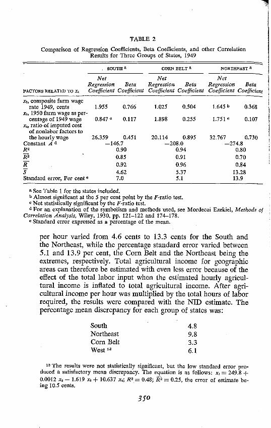
TABLE 2

Comparison of Regression Coefficients, Beta Coefficients, and other CorrelationResults for Three Groups of States, 1949

SOUTH a CORN BELT a NORTHEAST a

Net Net NetRegression Beta Regression Beta Regression Beta

FACTORS RELATED TO X, Coefficient Coefficient Coefficient Coefficient Coefficient Coefficient

X., composite farm wage1.025 0.504 1.645 b 0.368rate, 1949, cents 1.955 0.766

X" 1950 farm wage as per-1.898 0.255 1.751 e 0.107centage of 1949 wage 0.847 e 0.117

X" ratio of imputed costof nonlabor factors tothe hourly wage 26.359 0.451 20.114 0.895 32.767 0.730

Constant Ad -146.7 -208.0 -274.8R2 0.90 0.94 0.80R2 0.85 0.91 0.70if 0.92 0.96 0.84S 4.62 5.37 13.28Standard error, Per cent e 7.0 5.1 13.9

a See Table 1 for the states included.b Almost significant at the 5 per cent point by the F-ratio test.e Not statistically significant by the F-ratio test.d For an explanation of the symbolism and methods used, see Mordecai Ezekiel, Methods of

Correlation Analysis, Wiley, 1930, pp. 121-122 and 174-178.e Standard error expressed as a percentage of the mean.

per hour varied from 4.6 cents to 13.3 cents for the South andthe Northeast, while the percentage standard error varied between5.1 and 13.9 per cent, the Corn Belt and the Northeast being theextremes, respectively. Total agricultural income for geographicareas can therefore be estimated with even less error because of theeffect of the total labor input when the estimated hourly agricultural income is inflated to total agricultural income. After agricultural income per hour was multiplied by the total hours of laborrequired, the results were compared with the NID estimate. Thepercentage mean discrepancy for each group of states was:

SouthNortheastCorn BeltWest 13

4.89.83.36.1

13 The results were not statistically significant, but the low standard error produced a satisfactory mean discrepancy. The equation is as follows: x, = 249.8 +0.0012 x, - 1.619 x, + 10.637 X,; R2 =0.48; R2 =0.25, the error of estimate be-ing 10.5 cents. '

35°


Thc:se discrepancies are satisfactory, considering the limited dataavailable. The results are comparable to sampling errors found byactual field surveys of net farm income in Iowa.14 According toresults pUblished in 1942, the sampling percentage of average netcash income of farm operators varied between 8.8 per cent and 15.1pe~ cent for type of farming areas, with 5.9 per cent for the stateestimate.

For the South, the discrepancy of the estimate for 1949 from NIDestimates varied from -6.1 per cent for North Carolina to +10.3per cent for West Virginia, the mean discrepancy being 4.8 per cent.With the exception of West Virginia's 10.3 per cent, the individualstate errors cluster about the mean discrepancy quite closely, indicating a high degree of success in applying the regression equation.

PREPARATION OF COUNTY ESTIMATES 15

In preparing estimates of agricultural income of counties, theresults must represent the standing of the county in net income inrelation to other counties in the region. I think the regression methodemployed here meets this requirement sufficiently for practical useof the estimates. But in order to apply regression coefficients fromstate relationships to preparation of county estimates, two problemsmust be solved: the theoretical basis for the application of regressioncoefficients from larger geographic areas to smaller areas must beformulated, and a numerical series of independents for countiescomparable with those of the states must be secured.

Regression relationships of larger areas may be validly appliedto smaller ones because the input-output function in productionand income formation is not dependent on the size of the geographicunit. This assumption becomes of unlimited applicability even between firms and geographic units when rents and profits are includedas a part of the cost, as they are in x. (the ratio of the imputed costof nonlabor factors to the hourly wage). Because this factor reflectsinput combinations (and also weather and price influences throughtotal farm receipts) in dollars, the problems arising from variationsin both enterprise and expense mix. are avoided because all are inthe same unit of measure.

The second major problem, that the variables must be equallyavailable for both states and counties, was solved sufficiently for

14 Raymond J. Jessen, Statisticallnvestigatio1J of a Sample Survey for ObtainingFarm Factg. Iowa State College of Agriculture and Mechanic Arts, Research Bull.304. June 1942, p. 14.

15 The method is tested with Virginia counties because the basic labor requirements were worked out for Virginia counties in 1953. Clerical help was too limitedto perform an additional set of calculations for other states.

15'


the purposes of this study. X2 (composite wage rate) and Xs (1950wage as a percentage of the 1949 wage) were not available bycounties. Both factors, however, were ded~ced from data providedby the Department of Agriculture on April 1950 composite wagerates for economic areas. IS

In order to compute x., the ratio of the imputed cost of nonlaborfactors to the hourly wage, estimates of total farm receipts by coun·ties 17 were built up from census data, Department of AgriCUlturestatistics, and from data from the crop reporting service in Virginia.The total labor requirements fo~ all enterpri~es of each county werecomputed by applying the labor I~put per umt 18 to all acres of cropsgrown, livestock on farms, and lIvestock products. Total labor requirements for eac~ county were divided i~to t~e total farm re~eiptsto obtain farm receipts per hour. From thiS pomt, the calculatIOn ofx. for counties employed the same procedure as for states. The reosuIting county ratio for x. is therefore analogous to the state ratiofor X4-

The values obtained for X2 and Xa by economic areas made up ofseveral counties, however, are not directly analogous to thesefactors at the state level, but meet the requirements sufficiently. Itwould be preferable to have these factors for counties, but the errormade from employment of area measures probably does not materially affect the county results. Since economic areas were definedin tenns of economic factors, selected to meet a high degree ofhomogeneity, farm wages that resultfrom them are likewise expectedto be fairly homogeneous throughout the area. IS

IS Data on fann wage rates by economic areas are available from Special StatisticsBranch, Agricultural Marketing Service, Department of Agriculture. For definitionof economic areas, see Donald J. Bogue, "State Economic Areas," Dept. of Com·merce, processed, 1951, pp. 1-9.

17 Cash fann receipts 1D reasonably complete form are prepared by the cooperative crop reporting service of some states. In making application of the regressioncoefficients to a sample of twenty Virginia counties, however, it was necessary toadjust census reports of cash farm receipts to Department of Agriculture estimatesby a ratio method, adjusting each enterprise independently to reOect a maximumfor specialization. Estimates of value of farm products consumed on farms had tobe built up approximately from the census of 1945.

IS Labor requirements for most farm enterprises by states may be obtained fromDepartment of Agriculture reports as follows: Reuben W. Hecht and Keith R.Vice, Labor Used for Field Crops. Statistical Bull. 144, June 1954. and Reuben w.H~ht, Lobor Use~ for Livestock, Statistical Bull. 161, May 1955. For greater detaIl on I~bor req~rementsby type-of-farming arens, the applicable section of CropProdu.ctlOn PractIces: Labor, Power and Materials by Operation, F.M. 92, 19521953 IS recommended.

19 T!'ere is no good substitute for farm wage data by counties. but the area wage '--'dat.a gives a good. ide.a of the potentialities of the method. The use of the results asestimates can be Justified under present conditions because nothing better is avail·able.

JJ2


':!'he result.s of applying the regression equation to preparation ofa~c::ultu~al mcome for twe~ty counties, taken as a sample of Virgmla agnculture, are shown m Table 3.20 This table shows the 1947

TABLE 3

Comparisons of Estimates of Agricultural Income for Twenty Virginia CountiesPrepared by Different Methods, 1947 and 1949

19491947 1949 Estimates 1949 IncomeRatio Allocation Regression Total Formation

Area Estimate Estimate Estimate Receipts a Ratiosb

(thousands of dollars) (per cent)Accomac $11,325 $ 9,788 $ 9,699 $ 17,490 55.5Albermarle 4,097 2,735 3,818 6,453 59.2Alleghany 603 416 574 948 60.5Amelia 2,231 2,816 2,356 4,053 58.1Amherst 2,437 1,888 1,857 3,188 58.2Apr>mattox 1,853 1,787 1,573 2,699 58.3Arlington 56 34 70 121 57.9Augusta 9,820 7,893 9,379 16,142 58.1

Bath 990 661 843 1,414 59.6Bedford 4,294 4,473 4,599 7,899 58.2Bland 1,151 1,058 1,091 1,926 56.6Botetourt 2,919 2,728 2,807 4,828 58.1Brunswick 5,091 4,608 3,979 6,625 60.1Buchanan 1,298 1,734 1,335 2,219 60.2Buckingham 2,530 2,566 2,181 3,772 57.8

Camf1:ll 3,755 3,432 3,329 5,728 58.1Caro' e 2,251 2,394 2,353 3,984 59.1Carroll 3,234 4,118 3,570 6,358 56.1Charles City 872 878 833 1,558 53.5Charlotte 3,516 2,845 2,984 4,974 60.0

Total $64,329 $58,852 $59,230 $102,379 58.2

Counties as anarea c $64,335 $58,852 $59,231 $102,376 57.9

State $322,200 $297,500 $297,500 $516,900 57.6

Counties as per-centage of state 19.97 19.78 19.91 19.81

• Includes cash farm receipts plus value of products consumed on farm whereproduced. .

b Re~ession estimate of agricultural income as a percentage of total receIpts.c Estunate prepared by method shown for twenty counties treated as an area.

zo The calculation of the regression estimate will be illustrated for AccomacCounty, Virginia. Since Virginia was included in the South, the applicable regression equation is x, = -146.7 + 1.955 x. +0.847.ra + 26.359,x..

The values of the independents for Accomac County are: x. equals 52.2;.lO, 101.1;and x.. 3.54. Substituting in the equation: x. = -146.7 + 1.955 (52.2) + 0.847(101.1) + 26.359 (3.54). x. = -146.7 + 102.1 + 85.7 + 93.3 = 134.4 cents per

353


estimates, 1949 estimates prepared by two methods, total fann receipts for 1949, and the ratio of agricultural income formation for1949. The 1949 regression estimate was prep~re~ from the regres·sion equation for the South for 1949 by ap~hcatlo~ of the countyvariables discussed above. The 1949 al!ocatlon estimates was prepared by deducting from total farm receIpts all farm expenses, bothfixed and variable, which were calculated by numerous allocationprocedures, some based on data given in the 1950 census of agriculture and such prior censuses as were n~cess?ry to fill the gaps. Theresults are obviously only rough approxImatIons and are useful onlyin general comparis~ns with the regression estimat~ for 1949.

The regression estimates are preferable to the estimates preparedby allocation procedures from several standpoints. First, the alloca·tion estimate is subject to error due to the mixed use of farm capitalin some counties. In practically all farm counties, off-farm work,mainly in towns, is performed by farmers and farm laborers. Part ofthe investment in farm buildings, farm automobiles, and trucks ischargeable to off-farm work. This is also true of the maintenancecosts on all three items, and of gasoline, oil, and other operatingcosts on farm trucks and automobiles. To my knowledge, this mixeduse of farm capital is ignored by allocation procedures currently inuse. The regression procedure avoids this problem because the estimates are based on the value of inputs of laoor and its relation toother factors of production employed solely in agricultural production.

Second, the income formation ratios for 1949 conform moreclosely to a normal curve than the ratios from the allocation procedures. Despite the fact that the regression estimates of agriculturalincome per hour for twenty counties varied between 49 cents and152 cents per hour, the income formation ratios showed a coefficientof variation of less than 3 per cent, compared to 20 per cent for theallocation estimates. The abnormality of the latter estimates is further shown by the relatively large negative skewness. Theoretically,~e ratio of income formation should not vary greatly between countIes, since under competitive conditions, capital and other resourcestend to move to the more profitable counties, correcting most of thedifferential.

Third, relative variations between net income from the regressionestimates and gross income conform more closely to the generally

ho~r. The total 134.4 cents per hour gives $9,917,000, which required a downwardadjustment of 2.2 per cent to $9,699,000, in order to be in line with the twentycounty share of .the s~te ~ta1. This 2.2 per cent discrepancy happens also to equalthe error made m estimating the state total from the regression equation.

314


accepted theory of expected variations than variations between netincome from allocation procedures and gross income. Net incomeestimated from regression coefficients showed a coefficient of variation of 87 per cent compared to 83 per cent for net income estimatedfrom allocation procedures. The coefficient of variation of grossincome to which both are comparable was 81 per cent. Thus, therelative variability of net income derived from regression estimateswas substantially greater (7 per cent rather than 2 per cent) andtherefore in accord with theoretical expectations.

In the preparation of estimates of agriculture income of countiesfor 1947, a simple procedure was employed. The 1949 income formation ratio for each county (last column of Table 3) was adjustedfor the difference between the state income formation ratio for 1947and 1949, and the result was applied to the corresponding countyfarm receipts for 1947. This procedure is based on the assumptionthat differentials between county income ratios remain fairly constant during a period of two or three years. New enterprises areaccepted slowly on a wide scale. Shifts in the pattern of old enterprises in response to changes in prices do not seriously disturb therelationship, because resources are fairly completely utilized byenterprise substitutions.

Another problem is the relationship between the prices receivedby farmers and prices paid by farmers (the parity ratio). A changein this affects directly the level of income formation in geographicunits. Between any two years a rise in the parity ratio raises the rateat which income is formed; a fall lowers it. Such a change is reflectedin the NID estimates of state incomes and shows up clearly in income formation ratios for the respective states. The adjustment ofthe county income formation ratios was introduced to handle thisproblem. The income formation ratio of Virginia for 1947 was expressed as a percentage of the 1949 ratio. Since the ratio in 1947was 59.3 per cent and in 1949, 57.6 per cent, the percentage relationship was 103. Each county income formation ratio for 1949 wasraised by 3 per cent to obtain the estimated income formation ratiofor 1947 on the assumption that any regional differences in theparity ratio effects were adequately reflected in the respective stateincome formation ratios.

Application of the same percentage adjustment to each countyratio of the census year causes the absolute effect of the adjustmentto vary with the size of the county ratio. Thus, counties with low income formation ratios (high cost ratios) receive comparatively lessadjustments from ch~ges ~ the parity ratio .th~ the counti~ withhigh income formation ratios. The result IS m accord WIth the

JJJ


observed tendencies for counties with high ratios to be more volatile to inflation and deflation than counties with low income formation ratios. The adjusted ratios were ~pplied d~rectly to t?tal farmreceipts of counties for 1947 to obtam a.net m~ome estimate for1947 (first column of Table 3). The malO detaIls of the step involved in preparing the estimates are given in Tab!e 4.

The income formation ratio for 1947 was obtamed by multiplying the 1949 ratio by 1.03, derive~ fr0!D the state relationship between the two ratios (see the last hnes In Table 4). Total farm receipts were estimated from Department of Agriculture data byprocedures analogous to those used for the census year 1949, exceptthe nearest census distributions of receipts was the basic methodfor allocation of the Department of Agriculture estimates of receipts for intercensal years. The estimates of agricultural net income were then prepared by applying the 1947 ratios in the secondcolumn to total farm receipts.

The method is a rapid but crude procedure by which to obtainestimates for intercensal years with a minimum of labor. The in·come formation ratio for 1947 was 3 per cent higher than for 1949,reflecting mainly the difference in the parity ratio. Each county in·come formation ratio obtained by the more precise regression meth·ods applicable to census years was increased by 3 per cent. Thus,the ratio for Accomac county was raised from 55.5 per cent to 57.2.Total receipts in 1947 were $19,799,000; in 1949, $17,490,000.Therefore, the corresponding estimates of net income were $11,325,000 and $9,699,000. In other words, an increase in total receipts of $2,309,000 produced an increase in agricultural incomeof $1,626,000. The method will practically always produce esti·mates for intercensal years that vary in the same direction as totalreceipts, as do all twenty counties in Table 4. Other methods triedby the writer failed to do so consistently. Obviously, changes in taxesand contract interest, the only two overhead charges rigidly fixedin the concept of agricultural income here used, arc not fully reflected by this method. But the effects are minor in most counties.However, if desired, a separate adjustment could be attempted forboth items. Thus, the results, although rougher than estimates byregression equations (which could also be computed for intercensalyears), are restricted to uses where refinements in the series are not _required. The method should be a valuable aid, however, in pr0viding county estimates of agricultural income cheaply until bettermethods are developed.

In conclusion, I believe that the rearession methods that havebeen tested experimentally for one cens~s year (1949) and the one

356

TABLE 4

Agricultural Income for Twenty Virginia Counlies for 1947

Income Ratio E.ttimatedIncome Corrected Total Farm Agricultural

Area Ratio 1949 101947 Receipts 1947 Income 1947(percent) (thousands of dollars)

Accomac 55.S 57.2 $ 19,799 $ 11,325Albermarle 59.2 61.0 6,716 4,097Alleghany 60.5 62.3 968 603Amelia 58.1 59.8 3,741 2,237Amherst 58.2 59.9 4,069 2,437Appomattox 58.3 60.0 3,089 1,853Arlington 57.9 59.6 94 56Augusta 58.1 59.8 16,421 9,820

Bath 59.6 61.4 1,612 990Bedford 58.2 59.9 7,168 4,294Bland 56.6 58.3 1,975 1,151Botetourt 58.1 59.8 4,881 2,919Brunswick 60.1 61.9 8,224 5,091Buchanan 60.2 62.0 2,093 1,298Buckingham 57.8 59.5 4,252 2,530

Campben 58.1 59.8 6,279 3,755Caroline 59.1 60.9 3,696 2,251Carron 56.1 57.8 5,596 3,234Charles City 53.S 55.1 1,583 872Charlotte 60.0 61.8 5,689 3,516

Total $ 64,329

Counties as an area 57.90 59.60 $107,945 $ 64,335State 57.55 59.28 322,200

Counties as percentageof state 19.97

State ratio of 1949 to 1947 1.03

intercensal year (1947) point the way toward reasonably reliableestimates of agricultural income of counties. The methodology mayneed further refinements for some purposes. In any event, the procedure emphasizes the high importance of farm labor to incomeformation in agriculture. Considering the inadequate emphasis givenby the Department of Agriculture to the statistical coverage and reporting of farm wage rates of counties, the good results obtainedeven with an inadequate wage series show that the deficiencies insuch a vital set of agricultural data should be corrected. Equallyobvious, both the further refinement of the methods presented hereand their efficient use in the future depend greatly on accurate dataof unit labor requirements of farm enterprises, which data happilyhave been receiving increased emphasis from the Department ofAgriculture in recent years.

357


COMMENT

ERNEST W. GROVE, Agricultural Marketing Service,Department of Agriculture

For a number of years I have had intimate working contact withnational and state estimates of agricultural income. I know theirweaknesses, the numerous problems encountered in their development, and the large amount of work needed for their improvement,especially at the state level. Under the circumstances, I cannot quella feeling of impatience and frustration when I learn of the largevolume of work being done in the allocation of these inadequatestate estimates on a county basis.

Since last fall the Department of Agriculture has been reappraising its national estimates of farm production expenses and developing state estimates of production expenses. These will, in tum, permit reinstatement of the series on net farm income by states. TheNational Income Division of the Department of Commerce is alsoreappraising and revising its state income payment series, and wehave been cooperating in revision of the agricultural components.Therefore, state estimates both of total and of agricultural incomemay shortly be available on a more satisfactory basis than hitherto.

I also have an instinctive distrust of mechanical formulas of thetype proposed by John L. Fulmer. If, however, county estimates arereally required, then the difficulties of ordinary allocation proceduresare all too evident in the case of agricultural income. Any formulaor method that can either improve the accuracy of county agricultural income estimates or reduce the work required with no loss inaccuracy will clearly be worthwhile. In what follows, I shall try toshed my natural biases and consider Fulmer's method from thatstandpoint.

Although I cannot be sure, I do not think Fulmer's formula isproperly described as a work-saving device. For example, his methodrequires as a first step the multiplying out of all the unit labor requirements by acreage, production, or numbers of each commodityto get total man-hours of farm labor required in each county andstate. If I am right in concluding that the formula is not a sho~cut, then it must stand or fall on its merits as a device for improv-ing the accuracy of county agricultural income estimates. '--'~

I shall discuss each of the independent variables in tum. I haveno quarrel with X2, the composite hourly cash wage. Net agricultural income represents the net income of farm operators plus farm

318


wages, and it is not unreasonable to suppose that a total may becorrelated ~t least to .some extent with one of its parts.. ~ doubt ~f Xa, the mdex of wage change, is a significant variablem Its own rIght. At the county level, the absolute change in the composite hourly wage for the state as a whole had to be used for eachcounty, and the resu. that Xa turned out to be almost a constantat the county level insignificant as a means of differentiatingamong the various count. as to size of agricultural income.

The independent variable x. is what Fulmer refers to as theratio of wages to other inputs. It was derived, however, by dividing total gross receipts per hour by the hourly cash wage, and subtracting I from each of the resulting ratios. The final subtractionstep had no effect on x. as a variable in the regression analysis, soit may be considered simply as the ratio of gross receipts to cashwages.

Although I do not have the information necessary to prove this, Isuspect that the ratio of gross receipts to cash wages varied amongthe states in much the same manner as gross receipts alone. Or perhaps it varied more nearly like gross receipts minus cash wages. Butin either case, if the index of wage change were left out of theanalysis, then agriCUltural income would be correlated (1) with cashwages paid and (2) with gross receipts-all expressed on an hourlybasis. Reduced to its simplest terms, therefore, I think Fulmer'sanalysis correlates agricultural income with one of its parts and withthe gross total of which it is a part.

Fulmer provides a rationalization of his procedure, largely interms of the assumed working out of competitive forces in agriculture. Without going intorne pr,-'s and cons of this underlyingtheory, I think that a consi<'erable derree of correlation is to be ex··peeted in this type of 3I'JIysis. Yet I cannot share Fulmer's confidence in the predictiv,:- value of his fOl.nula at the county level.

He reports that we coefficients of currelation were statisticallysignificant for three of the four regions analyzed. But correlation c0

efficients that are significantly greater than zero are not enough forthis type of analysis. With only eleven observations for the southernstates, and with three independent variables used, my own feelingis that the correlation ought to have been practically perfect at thestate level before the resulting regression could be used with anyconfidence as a predictor of agricultural income at the county level.When there are so few observations, the theoretical basis for therelationship also should not be subject to any question.

I do not think that Fulmer's fonnula has met either of these tests.Nevertheless, he has used it to estimate agricultural income in


twenty counties of Virginia, and in about half of t~ese counties esti.mates based on the regression fonnula ar~ sigmficantly differentfrom estimates derived by the usual allocation procedures. Fulmercites the greater uniformity in ':income f~rmati?n ratios" as an in·dication of the superiority of hIs regression estimates. But there isno reason to suppose that the ratio ~f net to g.ross income is thesame or nearly the same, in the vanous counties. The possibility-indeed, the probability-of differences in this ratio is the essenceof the problem. Ordinary allocation procedures may lead in somecases to exaggerated differences in the ratios of net to gross income.But may not the regression method tend to understate such differ·ences?

On the whole, my conclusion must be that the formula is interest-ing and provocative, but certainly far from having been proved.But my suspicions concerning Fulmer's formula do not prevent mefrom concluding that it may be just about as good as any othermethod, if county inconle estimates have to be made. It may evenbe superior to the usual methods, as Fulmer claims. But that, I think,is the proposition that remains unproved, and personally I do notbelieve it.

Any method of allocating agricultural income by counties reomains somewhat suspect until its Validity can be proved beyondquestion. And it is not likely that the Validity of Fulmer's methodor any other method will be fully established until its results can betested against independent and reliable data on agricultural incomesin the counties.

Where are we going to get these check data? So far it seems tome that the very basis for proof has been lacking.

ROBERT H. JOHNSON, University of Iowa

My comments on John L. Fulmer's paper fall into three categories: those related primarily to the data problems, those relatedto the theoretical framework, and an evaluation of the results of theregression equation technique employed.

Data Problems

So !ar as I can determine from Fulmer's paper, the state agricultural mcome total being allocated by counties reflects cash receiptsfrom farm ma~keting flUS the value of home consumption. Apparently, there IS no adjustment for the fact that cash receipts maybe ~eater than, or less than, income produced in any given timepenod. The National Income I?ivision of the Department of Com'

360


merce state estim~tes, employed as a control figure, include thevalue of changes In f~rm inve~tories. Thus, there is a conceptualgap between the agncultural Income being allocated by Fulmerand the similar measure employed by the NID.

. Although there is ~o direct, easy solution to this problem, thediscrepancy may be lIDportant and the value of changes in inventory may not be spread uniformly among counties. Hence, astate control figure may be unsatisfactory. In a two-stage agricultural economy, such as Iowa, it is not uncommon for inventoriesof ~me ~roducts. (feed grains) to be changing in one direction,while the mventones of other products (livestock) are moving in theopposite. As some counties are predominantly specialized in one orthe other of these products, inventory Changes, by counties, cannotbe viewed as proportionate to change in inventories in the state asa whole.

While the choice of regional boundaries is apparently in somedegree arbitrary, placing in the same region such dissimilar agricultural economies as those of Kansas and Oklahoma, on the onehand, and Oregon and California, on the other, or Iowa and NorthDakota, leaves much to be desired. Fulmer's four-constant regression equation approach creates the dilemma that to obtain statistically significant measures of correlation the number of observations (states) must be kept fairly large, but to get enough states ineach regression, the regions must be so large as to cast serious doubtson the homogeneity of their agricultural processes and institutions.

In the absence of detailed county information on labor input,Fulmer's method relies on standard ratios for each state.1

Are such averages capable of reflecting the intrastate differentialsin income formation in agriculture? For example, the average manhour per acre ratio for corn in Iowa was 8.8 in 1950; in the adjacent states of Missouri and Minnesota the ratios were 14.3 and10.8, respectively. Yet, in the southern border counties of Io~a,

the input requirements are probably much closer to those of M~souri than to the state-wide average in Iowa. And the same condI-tion probably prevails on the n~rthe~ border.2

• •

The inadequacy of state-WIde ratIos of labor reqUIrements IS

somewhat obscured by the character of the estimating equation,in which labor hours required enters in as a divisor (in the computation of gross receipts per man-hour of la~r input), an~ as a multiplier (of net income per hour of labor mput). Thus, It seems to

1 In Virginia, separate ratios were aVailabl~ ~Y. crop districts."Labor requirement ratios for Iowa and adjOining states fro~ Reuben W. Hecht

and Keith R. Vice, Labor Used for Field Crops. Dept. of Agnculture, Bureau ofAgricuJiural &anomies, Stat. Bull. 144, June 1954, Table 3, p. 11.

361


make little difference in the final estimate of county income whatfigures are used for "labor r~quired." .Using t~e value of the coeffi.cients for estimation of agTlcult~ral m~ome !n ~ccomac County,Virginia, for example, if labor mput IS arbltranly reduced 18.7per cent, from 7,399 thousand man-hou~s (Fulm~r's estimate) to6 000 thousand man-hours, the total agncultural mcome estimatef~r this county is reduced b~ only.~.2 per ce~t .. A r~gression equa·tion that yields estimates so msensl~lve to va~latlons In values of theindependent variables may contaIn m~re Int~~al offsets than isconsistent with the proper degree of dIfferentiation among countyincome levels.

The whole estimating procedure would probably be improved ifthe "composite wage rate," X2, could be obtained by counties ratherthan by "economic areas" composed of several counties. For example, in s~me of these e~onomic ~r~as, st~ictly rural. counties arecombined With other countIes contammg major mdustnal employerswith effectively unionized employees. It would be surprising if farmwage rates were uniform in such nonhomogeneous labor markets.Again, however, the internal offsets in Fulmer's regression equation minimize the net results of differences in farm wage rates, including any errors arising from the use of average rates not typicalof particular counties. For example, if the wage rate used in Fulmer's computation for Accomac County is arbitrarily reduced by,say, 20 per cent (from 52.2 to 41.8 cents per hour) the total agricultural income estimate for the county is increased by 7.2 per cent,from $9,917 thousand, to $10,633 thousand.

The use of the state average rate of change in the ratio of income formation as an "adjustor" for each county may give distortedresults. If the product mix and the cost structure are highly uniformin all counties, the results from this method of preparing intercensalyear estimates are probably as good-or as bad-as the estimatesfor census years, or the years for which the regression equations arecomputed. But the ratio of prices received to prices paid by farmproducers does not change uniformly for all types of producers.Over short periods (and it is the short run which is relevant here),income per dollar of gross receipts may be changing at differentrates for producers of, say, feed grains and producers of cattle andhogs. If there is substantial specialization, by counties, the application of a state-wide rate of change in the income formation ratiogives distorted results.

The preparation of intercensal year estimates would be improvedby using a composite rate of change in each county. This compositewould reflect the change in the income formation ratio for each

362


major agri~ultural product, wei~hted acc~r~g to the composition~f output 10 .each county. Admittedly, this IS a more complicated,tiII1e-consumlOg process than that employed by Fulmer. But the results are logically defensible.

Conceptual Framework

Two assumptions appear basic to Fulmer's technique. First, thefacto~s of production must be combined in such proportions thatmarglOal returns per dollar of outlay are equated for all units ofinput-land, labor, capital, and management. Second, in order toapply the constants and regression coefficients derived from statedata for regions to the estimation of county agricultural income,the independent variables must have the same meaning when theyrepresent counties as when these independent variables representedthe several states composing the regions.

I think it is particularly hazardous to rely on the farm wage rateas a predictive device in the estimation of agricultural income bycounties on the ground that "the biggest share (around 60 per cent)of agricultural income goes to farm labor as earnings for labor."Available wage rate data are for explicit wage payments to hiredworkers, which account for from 15 per cent to 20 per cent of totalfactor earnings in agriculture.3 The 60 per cent return to labor isfrom two-thirds to three-fourths residual income. It is improbablethat "workers" shift from the status oflaborer to that of entrepreneurwith sufficient ease, and in adequate numbers, to make the explicitwage payment for agricultural laborers a reliable measure of therate of residual labor earnings from agriculture. lnimobilities attributable to inadequate capital, knowledge of alternatives, skillsrequired for farm management, and the limited supply of land available for laborers-turned-tenant raise serious questions on the efficacyof the price mechanism as a device for the equalization of factorrates of return-even in a competitive industry.

However, Fulmer's regression equation contains certain compensating features, since the composite area wage rate appears as anumerator in X2' and in both the numerator and the denominator inx,. Ceteris paribus, a lower wage rate will decrease the value ofX2 and increase the value of X4. Only if gross receipts per hour of(standard) labor input and the money wage rate of hired laborchange in the same ratio will the value of .t", be constant.

In terms of the theory of regional income formation, the most

I National Income Supplement, 1954, Survey 01 Current Business, Dept. of Commerce, Tables 13 and IS.

AGR.ICULTURAL INCOME OF COUNTIES

serious defect in Fulmer's technique is his use of the independentvariable x computed by counties with a coefficient derived from amUltipl~ c~rrelation analysis employing data for a number of notvery homogeneous states. Basically, x. i~ a computed "independentvariable," derived by dividing gross recelp~ per hour.of (standard)farm labor minus the wage rate for agrIcultural hired labor, bythe wage rate. Thus, x. is a ratio of nonlabor costs of production(including rents, interest, and imputed returns to management)to the hourly earnings of hired labor. But the x. variable isnot a ratio of other factor costs to labor costs, because the numerator includes all outlays, whether for factor costs or for purchases of intermediate goods. And this characteristic is true ofboth the state and of the county values of X•. But, unless the internal structure of the Xi variable is the same at both levels, i.e.unless the proportion of x.. accounted for by intra-area purc1uJsesof intermediate goods is the same for states and counties, the application of the state coefficient will not--even conceptually-yielda measure of factor earning accruing to farm labor and propertyresiding in the particular county.

In two counties having the same values of X2' Xa, and x.and hence the same values for net income per hour-the ratio ofnet agricultural income to gross receipts may be very different, depending upon the proportion of the x. representing returns tofactor owners other than hired labor compared with the share of x.representing purchases of intermediate goods which mayor may notgive rise to factor earnings from agriculture, in the particular countiesfor which estimates were being made.

In the larger regions from which the regression coefficients werecomputed-and even in a state as a whole-the ratio of factor tononfactor costs embodied in the x. may be characterized by unifonnities not present in the ratio for individual counties. For onething, sales by one farm unit of, say, feeder cattle, feed grains, orhay, to another farm unit may be intraregional or intrastate, butare much less likely to be intracounty. Thus, x.. may represent varying amounts of factor returns to other than hired labor, dependingupon the relative importance of intermediate purchases containedin ~e ratio. In addition to the tendency for transactions with unitsoutside the area to increase as the size of the economic area is reduced from region to state to county, the stability of mass data foran area as large as a state can be expected to make for a greaterdegree of uniformity in the composition of x. for different states,than for different counties, even in the same state.


Evaluation of the Estimates

~or the tw~nty Virginia ~ounties f?r which ~ulme~ has computedagr:cultural mcome by hIs regressIon equatIon With coefficientsdenved from eleven southeastern states, the ratio of income formation to gross receipts is remarkably stable. Fulmer finds confirmation of tb:e validity of his es~imating procedure in the consistencyof the ratIo. I do not share hIS assurance that the uniformity of theinco~e ~ormati?n ratios. from co~nty to county demonstrates thesupenonty of his regressIon equation technique over the somewhatcumbe~ome, less formally precise allocation techniques widely employed m the preparation of county agricultural income estimates.

In his own estimates of county agricultural income by the allocation method, the range of the income formation ratio (excludingArlington County) is from about 42 per cent of gross receipts toalmost 80 per cent of gross receipts, or approximately a I to 2 ratio.In estimates of agriCUltural income for the ninety-nine counties ofIowa for 1939 (using concepts essentially the same as those employed by Fulmer), I found that income fonnation as a percentageof gross receipts ranged from about 44 to 74 per cent, a ratio of1 to 1.7. As might have been expected, the lower limit of the rangewas observed in a county specializing in the fattening of purchasedfeeder cattle, primarily with purchased com; the upper limit, in acounty located in the "cash grain" area. Even among states, agricultural income formation as a percentage of gross receipts rangedfrom about 30 to almost 70 per cent, or a ratio of I to over 2.

The uniformity of Fulmer's county ratios of agricultural incomeformation to gross receipts is attributable to several features ofthe estimating procedure. As already noted, the x, independentvariable does not reflect the substantial differences in the proportionsof factor to nonfactor costs. By applying the coefficient computedfrom state data to the independent variable based on county data,real county-to-county differences in income formation ratios maybe obscured. Secondly, substantial differences in th~ values of.thewage rate variable and in the hours of labor reqUIred have httleeffect on the final income estimates because of internal offsets that,together, comprise powerful "built-in equalizers" of the incomegross-receipts ratio. The labor input r~quirements seem .to be pa~

ticularly powerful in this respect. Despite a broad range m the es~l

mates of net income per hour of farm labo.r ~ro~ghly a 3 to I ratiofor the twenty Virginia counties) the multiplIcatIon of these hourly

36$


estimates by labor requirements eliminates most of the differentialsin the income-gross-receipts ratios.

Finally, on Fulmer's statistical technique, the regression equationcomprises three "independent variables." Yet, one of these variables(x2 , the hourly wage rate) enters directly into the computation ofthe other two. I am notsure in what sense the three variables can besaid to be independent. Certainly they are not independent of oneanother. It may also be questionable whether or not a coefficient ofdetermination (R 2 ) computed from such an equation can be evaluated in terms of the usual criteria.

EDWARD F. DENISON, Department of Commerce

My brief comment is confined to the theoretical basis offered byJohn L. Fulmer for expecting a high positive correlation amongcounties between the average wage rate and the value of total factorincome per man-hour worked.

Customary theoretical analysis would assume the existence of geographical mobility of farm labor, and hence a tendency for wagerates (and the marginal value product of labor) to equalize amongthe counties of a state. A similar tendency toward equalization ofinterest return would be assumed, while the entire differential return resulting from differing qualities of the land and from locational factors would, following the Ricardian analysis, appear indifferences among counties in the amount of economic rent. Statistically, economic rent appears in the income data as either rentalincome or farm proprietors' income.

In equilibrium, therefore, according to customary economictheory, the labor return per unit of labor would be equal in allcounties (except for the influence of non-wage-rate advantages anddisadvantages of the location) while the nonlabor return would beunequal, and no stable relationship between labor and nonlaborreturns would be anticipated. The differences in wage rates amongcounties upon which Fulmer relies would, from this approach, bepresumed to result from immobility and other imperfections in thelabor market and to bear no necessary relation to nonlabor returns.It seems to me that Fulmer needs to supply a reconciliation of hisviewpoint with the conclusions reached by other theorists.

JOHN A. GUTHRIE, State College of Washington

John L. Fulmer has prepared an interesting and provocative paper on a difficult subject. He has used some ingenious methods of

366


obtaining an estimate of agricultural income. His approach is alsointriguing because he uses economic theory as a basis for arrivingat his results. However, he makes a number of assumptions thatstrike me as being questionable, particularly when his theoreticalmodel is applied to specific situations.

He states that the relative productivity of labor as exhibited infarm wages is the source of differentiation between agriculture andthe rest of the economy, and also within agriculture between geographic areas. He assumes that all farm labor is paid its marginalvalue product and that the operator is paid for his labor at the samerate as hired labor. In other words, he seems to say that the wagespaid to hired labor in agriculture give a measure of labor returns tomanagement. I question these assumptions, particularly if appliedto areas where farm income is very high, and there are many suchareas in the state of Washington. Is the farm operator likely to pay,in each small area and under all circumstances, the marginal valueproduct to his laborers? Fulmer says this will be true because, if thefarm laborer is not paid the full marginal value product, he will become a renter. In the area of which I speak, renting is difficult. Thereis little rental land available and the renter must supply the necessary equipment, which may cost $30,000 to $40,000. Most of therenting is done by farm operators who already have a farm and whorent a piece of adjacent land.

I also question his assumption that, when conditions outside agriculture affect the price of farm products and raise or lower correspondingly the marginal value product of labor, the change in income is reflected in the asking price of labor and the bidding priceof farmers for labor. In the part of the country of which I speak,the farm operator has to bid against industrial plants, such as BoeingAircraft, Kaiser Aluminum, and others. But if the price of farmproducts goes up considerably while general wages in the area donot, farm laborers do not necessarily get any higher wages. Similarly,if farm income declines, the farm operator still has to pay the opportunity cost to attract the labor he needs. Fulmer agrees, ofcourse, that farm wages do not fully reflect the marginal valueproduct for farm labor because of contractual inflexibilities in wagerates, but he assumes that corrections are made when the wage ratesare renegotiated the following year. It seems to me that there maybe wide changes in farm income not reflected appreciably in thewages of farm labor.

His assumption that farm wages are a proportion of farm incomemay be true as a generality, but I question whether it should be usedas a basis for estimating income between counties or between dif-

367


ferent types of agricultur~. Also. the assu~ption of the completesubstitutability of factors IS somewhat questionable. Generally, thefann operator has a certain amount of equipment and hires a neces·sary amount of labor. If the price o~ labor g~ down somewhat, hemay hire some additional labor, or If the pnce ~f labor goes up, hemay hire less. But if hiring another man requires the purchase ofa substantial amount of equipment, he may not make any suchadjustment.

I wonder also how some of the factors needed in Fulmer's equa-tion are secured for intercensal years, for example, the x. factor inthe equation, the ratio of labor input to the computed cost of otherfactors. Is one to assume that the ratio is the same in each countyfor all years? If that is the assumption, I think it highly questionable. Also, how are the total hours of farm labor worked in eachcounty obtained from year to year? This information is crucial tothe use of the formula. Assuming that total hours of labor can becomputed for a census year, they may change considerably.

Fulmer also points out that it was necessary to build up estimatesof total farm receipts by counties from census data. This informa·tion is not normally available by counties for other than censusyears. He also says that it was necessary to compute total labor reoquirements for all enterprises in the county by applying the laborinput per unit of all acres of crops grown and livestock products.Again, how is this information obtained for other than census years?He says that the composite wage rate, unavailable by counties, wasavailable by economic areas from the Department of Agriculture.However, the economic areas frequently comprise a group of coun·ties, and in my state these economic areas do not necessarily com·prise counties that are homogeneous from an agricultural standpoint. In short, Fulmer's method raises a number of questions. Somepertain to the validity of applying theoretical models to actual con·ditions; others, to the lack of data to do the sort of thing that hewants to do. To apply his method. dependence must be put on dataobtained in census years which are not necessarily applicable tointercensal years.

Fulmer states that the series he gets for county income paymentsis more consistent than the estimates prepared by allocation procedures based on rough and inexact methods in calculations of expenditures. I think that the very nature of his estimating procedurema~es the ~esults .more .consistent. Does it necessarily follow that asenes that IS conSistent IS better? I am inclined to doubt this. Theremay be wide variations in the agricultural income of counties from

]68


year to .year because of variations in price, or of droughts, or ofother things.

REPLY BY THB AUTHOR

I am glad ~at Ernest W: Grove commented on the inadequacyof.the st.ate estimates of agncultural.income. I had come to suspectthis dunng the course of my analysiS. Obviously, if the basic dataare inadequate, highly significant results cannot be obtained byany method, and the one I described will not have a fair test untilthe greatly improved data he promises are available.

But those of us in the South and elsewhere who labor on economicdevelopment at the local level must proceed with the methods athand. Often a series must prove its usefulness before it can securethe financial support necessary for its refinement. Sales Management 1 has been pUblishing county income estimates annually sincethe 1930's. !hey are of the roughest sort, yet they are constantlyused by busmessmen and others to reach important decisions. Mymethod attempts to improve the farm income component of thatseries until a better method is developed or the proposed one refined.

Grove recommends that X3 be omitted because it made little contribution to the county estimates. This was true for 1949 to 1950,when farm wages rose only 0.6 cents per hour. Had tbe wage serieschanged by 5 to 10 cents, as it did in 1951, X3 would have made asignificant contribution. The factor was retained because of thiscontingency, and also to give a more refined net value to X2 and x•.

With regard to x., which reflects the relationship of the value ofthe imputed cost of other factors to the hourly farm wage, he concludes that it measures about the same thing as gross receipts on anhourly basis. This is an important misconception, because the formeris a relative while the latter puts the factor in terms of dollars andcents. By actual trial, x. was found to be both more highly relatedto the dependent variables than total hourly receipts and moreconsistent in its behavior between regions.

Grove considers the coefficients of determination unsatisfactoryfor predictive purposes in view of the small num~r of states re~re

sented in each case. However, since the coeffiCient of correlationwas statistically significant at the 1 per ceD;t lev~l f?r ~ee of ~eregions, the existence of a functional relationship is satiSfactorilyestablished. Reliable estimates depend on the scatter of the dataabout the mean relative to the slope of the line.! By this test, the

1 See Salt! Managemellt: Survey of Buyillg Power, May 10. 1953. pp. 20-27.2 See Mordecai Ezekiel, Methods of Co"elJJtioll AMly";,, Wiley. 1930. p. 138.


equations for all four groups of states gave good estimates, varyingfrom 5.1 to 13.9 per cent. The r~ther hetero~eneous group ofwestern states will produce good estimates also wIth a 9.2 per centerror, because the variance about the mean of the individual stateswas comparatively small.

I wrote that the greater uniformity of the county income formation ratios obtained by the regression method than by the allocation method showed that the first procedure is better. Grove, RobertH. Johnson, and John A. Guthrie either question whether this uniformity has any bearing on th~ validit~ of the method or considerthat it discredits the method, smce a high.degree of uniformity ofincome is not. to be ex~c~ed among counties. Pa~t of the diffiCUltyarises from. d~erences In mcom~ con~epts.. My discussants are apparently thmkmg of farm proprIetors net mcome, but my agricultural income concept is both broader and more refined than this. Iexclude rents paid farm landlords, wages to hired help, governmentpayments, and also errors that may occur in estimating these components.

I used this concept to get a measure of income consistent withfactorial earnings in the agricultural industry itself. Since the amountof tenancy and of hired labor varies greatly between states, theseadjustments should make for greater uniformity in the incomeformation ratios. This is exactly what happened, as shown by thepercentage variations of the ratios in 1949:

Northeast Corn Belt South WestAgricultural income •

Mean 38.86 44.11 57.74 50.07Standard deviation 5.18 3.78 3.97 8.69Coefficient of variation 13.3 8.6 6.9 16.2

Farm proprietors' Det income t.Mean 24.44 37.34 47.84 36.46Standard deviation 6.84 4.28 5.33 9.57Coefficient of variation 28.0 lI.5 II.l 26.2

. • The concept .a~ ~efined in this paper. Farm proprietors' net income of the Na·llo.nat Income Dlvlslon of the Department of Commerce, adjusted by adding renbpaid farm landlords plus wages paid hired labor. Government payments are de·ducted.

b Farm proprietors' Det income as defined by the NID.

The coefficient of variation of agricultural income is 25.2 to 52.5per cent less.than the variation of farm proprietors' net income. In?<>~ c~mpaflsons, the Com Belt and the South are substantially less,mdlcating greater homogeneity in their income formation ratios.

37°


In both concepts, however, the mean of the income formation~atios vari~ greatly ~tween !egions. Institutional factors may beun~rtant m e~plammg the ~ifferences among geographic units intherr rates of mcome formatIon. Had the concept of agriculturalincome been further refined to allow for rents paid to nonfarm landlor~ and interest paid for capital obtained outside agriculture, theratIos would have been even more uniform.~other !actor ~esponsi?le for the greater uniformity of the re

gressIOn estImates IS the mIXed nature of resource use in numerouscounties. The typical allocation procedures make no allowancefor the share of the expenses for maintenance of buildings and therepair, maintenance, and operating expenses on automobiles andtrucks that are chargeable to the activities of farmers away fromtheir farms. Without an adjustment for this outside activity, thereported total farm receipts of the counties are too low (39.9 percent of the counties reported off-farm work by farm operators in1950).

Also, if industrial and other employment opportunities exist inor near a county, the land and buildings carry an inflated value andare not properly sensitive to bona fide farm earnings in the capitalization process. This raises the rate of charge against receipts andmakes it inflexible. The Census Bureau procedure of valuing farmland and buildings by estimating the selling price of a sample givesan average of farmers' opinions over a period of years. The valuation will consequently not be sensitive to the current rate of earnings from farm operations. This leads to further error in the imputed charges deducted from farm receipts.

However, the appearance of uniformity of the income ratios canbe misleading. While the twenty counties were take~ as a sample ofVirginia agriculture, ~ey are not fully repr:sentatIve o.f t~e state,as shown by the followmg percentage coeffiCIents of vanatlon:

Coefficient of Variation:

0.1

43.1

1.6

11.1

Eleven TwentySouthern States Virginia Counties

Xl' Agricultural income per hour 18.0 34.1X" Composite wage rates per hour 11.6 10.5x.. 1950 composite wage as per

centage of 1949 wage%I, Ratio of imputed value of

other costs to 1949 wage

The twenty counties vary less in X2 and X3' but substan~ially morein x than do the eleven states. Although data are available onlyby ~onomic areas for X2, the coefficient of variation of wages for

37'


the ten economic areas of Virginia was 13.7 per cent compared toto.5 per cent for the twenty-county ~ample, indicating. 23 per centless variation than in the factor st~dled by the reg~esslon analysis.Since x accounts for about two-thirds of the coefficient of determi.nation :nd is jointly.re.latOO to x., its low~r variability bec~mes ~gh1yimportant in explammg .the comparatively gr~ater ~m.fomuty ofthe income fonnation ratio of the sar.np~e. counties. It IS mteresting,however, that despite the smaller vanablhty.of two of the Variables,agricultural hourly income was nearly twice as variable for thetwenty counties as for the eleven states: the range of hourly earnings of the twenty counties was from 151.6 to 48.9 cents comparedto 78.1 cents for Virginia. One expects greater variation in hOUrlyearnings as the size of the geog~ap~ic un!t decreases: it. is a bigfactor in favor of the fonnula that It gives this result. There IS dangerof forgetting this and concentrating too much on the income forma.tion ratio. Finally, to return to the question of the value of Xt in theequation, the very large variability for the twenty counties showsthe power it possesses to reflect extreme variations in the total receipts of small geographic areas.

I wish to comment on a few points raised in Johnson's criticalanalysis of my paper. First, my fonnula assumes that the state inventory adjustment rate can be used a<; the adjustment rate for thecounties. Obviously, this is an oversimplification. Perhaps inventorycharges should be adjusted independently where they are importantand particularly volatile, as in a grain and hay state such as Iowa.

Next, labor requirements should, of course, be calculated asaccurately as possible, particularly for counties. However, the lackof annual, current labor data is not important, since the incomefonnation ratio method obviates the use of labor requirements inmaking estimates for intercensal years.

Johnson is correct in stating that errors in the computation of Xt

may be largely offset by the interrelationships between X2 and Xt.

He arrived at this conclusion by arbitrarily changing the labor inputof Accomac County to test the effect on agricultural income. Whentotal labor requirements were reduced by 18.7 per cent, the estimate of agricultural income was reduced by only 2.2 per cent. Thisresult seems startling. But, if he had included an increase in wages,a n~ary co?dition to a reduction in labor input, the estim~eof agnculturalmcome would have been raised, not reduced, as hislater calculation shows.

Johnson questions whether the factors are independent of one

372


another. Conceptually, they were not intended to be so, since it isassumtd that the factors combine in a joint function to oive something more than. a linear~ additive function. He alsooquestions~hether chang~ m ~e panty r~tio can be applied uniformly to themcome fonnatlo~ r~tlo of ~untles in adjusting from censal to intercensal y~ars. ~1S IS a se~ou~ challenge to a basic assumption of!ann poh~y as.1t oper~tes lD th~ country at present. The same paritymdex (With ml~or adjustment lD the base for some crops) is appliedto all crops uniformly regardless of location in the calculation ofparity prices and price supports on the assumption that prices andcosts in different regions of the United States move together to suchan extent that the aberrations are minor.

However, the method outlined for intercensal estimates is notso hide-bound by this assumption as Johnson believes. While shiftsin the parity ratio from year to year are the major force causingchange in the income formation ratios between years, the adjustment percentage was not computed from the changes in the parityratio but from the changes in the income formation ratios of therespective states. To the extent that agricultural income accountingby states was based on a separate determination of individual components of expenses and receipts, the effects of the chan~es in theparity ratio were differentiated to the individual states and thereforewere reflected in the income formation ratios.

Both Johnson and Guthrie question the applicability to agriculture of the equimarginal assumption, holding that resource allocation operates imperfectly between agricultural and nonagriculturalenterprises and also within agriculture. But the well-known differential between farm and city wages is largely or completely compensated for by the tangible and intangible difterences between thecountry and the city. Farm perquisites are valued at farm pricesand not at retail prices. The required standard of life permits cheaperliving in the country than in the city.3 Some may place even ~ore

importance on the intangible values of farm life. But other thingsbeing equal, the farm to city migration picks up as the ~age differential widens, although some authorities who have studied the matter place more emphasis on employment.opportunities.4 1fthe.f~~rhas to bid higher for labor, h.e selects It more .carefu~y, utilizes Itmore efficiently, and adds capital. He has to adjust all mputs to the

• Paul D. Converse, Harvey W. Huegy, and Robert V. Mitchell, The Elementsof Marketing, .5th ed, Prentice-Hall, 19.53, p. 3.5.

'See Howard L. Parsons, The Impact 0/ Fluctuat!0ns. in NatioryailncfJme onAgricultural Wages and Employment, Harvard Studies m Labor m Agncu1ture,June 1952, pp. 36-46.

373


point where a dollar of outlay in every direc!ion ret~rns the samemarginal value product. He may. not do thIs conscIously or accurately, but competition makes th~s t!ue for farmers as a group.

Obviously, the equimarginal prmclpl~ d?es no! work perfectly;it is only necessary, however, that th.e ~nnclple eXIst as a .dominantforce for it to have value as a predIctIve factor. That thIs has occurred even in the state of Washington is indicated by the numberof farm operators working in industry and the number who aretenants.

Johnson places great emphasis on the fact that, even thoughabout 60 per cent of all farm income is allocable to fann labor, including the labor of farm operators, ~nl>, 15 to 2.0 per cent is paidout for hired labor. I contend that thIS IS a sufficIent percentage tomake the principle operative. Less than that percentage of thegreat American crop, corn, is sold, yet no one has ever questionedthe market value of the remainder.

One final comment on Johnson's discussion. He is disturbed thatthe proportions of the imputed values of other factors, including intermediate goods, rents, interest, and returns to management, expressed as a ratio to farm wages, varies between states and betweencounties. He believes this variation invalidates the use of X4 as apredictive factor. Production e.eonomics indicates that numerouscombinations of factors maj be used to obtain a given product.The important objective is ~o get production that returns opportunitycosts to the diJferen~ f~c~ors. There are obviously limits to substitution, but within them variations in the combination of factors between industries and between farms occur. Intermediate goods maybe substituted for land or fixed equipment. Such inputs as fertilizer,seed, fuel, and numerous others are used up in the process of production. Even where there are monopoly elements present, will notthe capitalization process cause the assets to take on the additionalvalue to represent the difference? It is apparent, therefore, that theinput mix, like the output mix, becomes homogeneous through itsdollar denominator. The ratio of other factors to labor provides amajor point of differentiation in view of the relative importance oflabor. My contention is that, for estimating purposes, it is all thedifferentiation needed.

Den~n suggests that I provide a reconciliation of my theoretical~odel WIt? that of conclusions reached by other theorists. My viewIS that agrIcultural income of counties is a function of the composite~ourl! ~age rat~ and .two other factors that influence the dependentID a Jomt functIon Wlth the wage rate. The basic postulate is that

374


~ann la~r, as a participant in production, receives approximatelyIts mar~1Dal value product. Denison states that under customaryeconomIc theory only land rent would reflect a differential betweencounties, being dependent. upon locational and productiVity differen~. Under the assumpt~on of geographic mobility of labor andcapital, the us~al theory 8lmS a~ equality of both interest and wagereturns per uOlt between counties.

In actual practice, the f~er with investments in land capitalizesthe rental re~. Thus, ~ an ent~epreneurial sense, the farm op~rator lumps ~vestm~nts ~ land WI~ other capital outlays, adjustmg the facton.al c?mbmatlon to eq~al~e marginal returns per dollarof outlay, takmg mto account the llIDlts of substitution between thetwo factors and each with labor independently or in combination.

Farm labor, whil.e som~what immobile in farm to industry movements because of mtanglble values associated with farm life, is,however, highly mobile between farms and between communities.Beyond counties, the mObility of farm labor drops rapidly. Despiteimperfections in the mobility of farm labor and the fact that only15 to 20 per cent is employed as hired labor, I consider that there issufficient mObility and bargaining over wages in labor contracts tomake the marginal productivity principle effective. With land andcapital treated in the same way by the entrepreneur through the capitalization process, it appears that the only fixed factor is the entrepreneur. He adds factors in the proper proportions until he maximizes entrepreneurial returns. Of course, the entrepreneur almostnever makes full utilization of his capacity because of capital rationing. I believe what I have said to this point is in accord generallywith economic theory.

Now to the problem of explaining the differences in wages between counties. Equality of the marginal value product of laborwithin a geographic unit requires that the labor unit be of equ~l

quality, an assumption violated in agriculture. The ~asic labor. umtis far from equal throughout agriculture because of inherent.~erences of ability and education within the labor force. The pnnclpalreason farm wages averaged in 1949 only 40.3 c~nts in the Southcompared to 70.9 cents in the Corn Belt was the difference betweentypes of labor. . . . .

The dilution of the labor force that accompanies mIgratiOn IS

also a significant source of county differentials. ~e more alertand intelligent laborers, who are also the most effiCient, m~ve firstand farthest.5 In the process, they move into types o! agnculturewith a better market advantage, as dairying, or more highly mecha-

I Ibid., pp. 36-46.

17$

AGRICULTURAL INCOl\IE OF COUNTIES

nized. This gives rise to county differentials within states and regionsand between regions.

In my model, I did not intend.to exp~ain the county differencesin income entirely by the wage differential, because the volume ofwork and other inputs vary so widely between counties. I had refer.ence to the hourly agricultural income, and even in this connectionthe model would be equally applicable if there were no labor differ.entials between counties. The three factors, especially because ofthe joint functions in which they are defined, are capable of a greatvariety of combinations and therefore widely varying agricultural in.come per hour between counties.

Guthrie is correct in his conclusion that I assumed that fann laboris paid its marginal product, but not that the "wages paid to hiredlabor in agriculture give a measure of labor returns to management."Returns to management include two components, the wages earnedby the operator as a laborer and the return he gets in his capacityas a manager. The wages of hired labor determine the lower limit~

of operator's returns. Operator's returns would average higher thanthe wage returns of laborers, rising with the level of fann wagesand conversely. There are geographic areas and circumstances wherethere may be little or no relationship. as in the state of Washington,but in general throughout the United States, they vary together.

measurement of agricultural income of counties - the national bureau of economic research ·...

Documents