measures and methods for reliable information processing · figure 24 nokia here example ......
TRANSCRIPT

GRANT AGREEMENT No 609035
FP7-SMARTCITIES-2013
Real-Time IoT Stream Processing and Large-scale Data Analytics for Smart City Applications
Collaborative Project
Measures and Methods for Reliable Information Processing
Document Ref. D4.1
Document Type Report
Workpackage WP4
Lead Contractor UASO
Author(s) D. Kuemper, T. Iggena, M. Bermudez-Edo, D. Puiu, M. Fischer, F. Gao
Contributing Partners UASO, UNIS, SIE, NUIG
Planned Delivery Date M18
Actual Delivery Date M18 (2015-02-27)
Dissemination Level Public
Status Completed
Version V1.0
Reviewed by João Fernandes (AI), Sefki Kolozali (UNIS)
D4.1 Measures and Methods for Reliable Information Processing – Dissemination Level: Public Page I
Executive Summary
CityPulse provides a framework for innovative smart city applications by adopting an integrated
approach to the Internet of Things and the Internet of People. Due to the heterogeneity of data
sources in those environments and the growing participation of citizens in social media, technical
reliability, logical inconsistency and trustworthiness of data are key challenges in providing stable
applications. Determining and managing provenance and trustworthiness of information sources is
an important step towards safe and secure operation of smart cities. This report describes
approaches for reliable information processing in smart city infrastructures. It proposes an ontology
based quality annotation for data streams, which utilises normalised quality metrics to gain an
application independent and comparable view of information quality. Different approaches to
measure the information quality of data streams are described. The analysis of a single data stream
utilises mutual information and Reward and Punishment algorithms to overcome limitations of
common approaches like Pearson correlation. Sensor readings of multiple spatio-temporal
correlated streams are evaluated by comparison against information sources, which capture similar
data, either streamed or event based. The quality evaluation of individual data sources is
demonstrated on a reference dataset. The evaluation reveals smaller defects in the data sources but
it also highlights correlations between different streams, which confirm the correctness of detected
events. The presented fault recovery concept proposes a value estimation approach to recover from
missing data.
D4.1 Measures and Methods for Reliable Information Processing – Dissemination Level: Public Page II
Contents 1. Introduction .................................................................................................................................... 1
2. Requirements .................................................................................................................................. 2
2.1 Quality Annotation .................................................................................................................... 2
2.2 Quality Analysis ......................................................................................................................... 3
2.3 Conflict Resolution and Fault Recovery ..................................................................................... 3
3. State of the Art ................................................................................................................................ 5
3.1 Information Quality Annotation ................................................................................................ 5
3.2 Information Quality Analysis ..................................................................................................... 6
3.3 Conflict Resolution & Fault Recovery ........................................................................................ 8
4. Quality Metrics for Reliable Information Processing .................................................................... 10
4.1 Data Stream Quality Definition ............................................................................................... 10
4.2 Annotating Data Stream Quality ............................................................................................. 13
4.3 Influence of Provenance .......................................................................................................... 15
5. Methods for Reliable Information Processing .............................................................................. 17
5.1 Utilisation of Available Information ........................................................................................ 17
5.2 Reference Datasets .................................................................................................................. 19
5.3 Single Stream Data Analysis .................................................................................................... 20
5.3.1 Spatio-Temporal Correlations ....................................................................................... 20
5.3.2 Reward and Punishment Algorithm .............................................................................. 25
5.3.2.1 Reward and Punishment Evaluation on Reference Data .............................................. 26
5.4 Multiple Stream Data Analysis ................................................................................................ 29
5.4.1 Effects of Different Window Sizes ................................................................................. 30
5.4.2 Impact of Different Features ......................................................................................... 32
5.5 Dynamic Semantics for Smart City Data in Constrained Environments .................................. 34
5.5.1 Experiment Setup .......................................................................................................... 36
5.5.2 Experiments .................................................................................................................. 37
5.6 Aggregation of Information Quality ........................................................................................ 43
5.6.1 Propagable Quality Metrics .......................................................................................... 43
5.6.2 Quality Aggregation ...................................................................................................... 44
6. Conflict Resolution & Fault Recovery ........................................................................................... 46
6.1 Fault Recovery ......................................................................................................................... 47
6.2 Fault Recovery Workflow ........................................................................................................ 48
6.3 Missing Values Estimation ....................................................................................................... 48
7. Implementation ............................................................................................................................ 52
7.1 Components/Architecture ....................................................................................................... 52
7.2 Workflow ................................................................................................................................. 54
8. Conclusion and Outlook ................................................................................................................ 57
9. References .................................................................................................................................... 58

D4.1 Measures and Methods for Reliable Information Processing – Dissemination Level: Public Page III
Figures Figure 1 Reliable Information Processing Integration in the CityPulse Framework ............................... 2
Figure 2 Quality Ontology ..................................................................................................................... 13
Figure 3 Quality Ontology in Protègè .................................................................................................... 14
Figure 4 Reputation Use Case ............................................................................................................... 15
Figure 5 Occurrence of High-Level Information .................................................................................... 18
Figure 6 Overview and Detailed View of Traffic Sensors in the City of Aarhus, Denmark ................... 19
Figure 7 Example Dataset (ODAA Traffic) ............................................................................................. 19
Figure 8 Quality Analysis - General Approach....................................................................................... 20
Figure 9 Block Diagram of the Methodology to Calculate Data Stream Movements ........................... 22
Figure 10 Four Weeks of Traffic Data Divided in Overlap Windows of 50% ......................................... 22
Figure 11 StreamA and StreamB to be Correlated in Time t ................................................................ 23
Figure 12 StreamA and StreamB to be Correlated in Time t (shifted) .................................................. 23
Figure 13 Location of Two Sections (A and B) of the City Traffic .......................................................... 24
Figure 14 Three Sections of the Traffic Data of Aarhus. ....................................................................... 25
Figure 15 Histogram Distribution of Frequency QoI Value Classes ...................................................... 27
Figure 16 Average Frequency per Sensor ............................................................................................. 28
Figure 17 Sensor Node Measuring Direction ........................................................................................ 28
Figure 18 Example Evaluation of Stream Data for Correctness Using Redundant Sensors .................. 29
Figure 19 Histogram Distribution of Correctness QoI Value Classes .................................................... 29
Figure 20 Scatter Plot where Pearson Correlation Fails to Find the Correlation. ................................. 30
Figure 21 Scatter Plot where Pearson Detects Some Correlation. ....................................................... 30
Figure 22 Mean and Variance of the Mutual Information and Pearson Correlation Results ............... 31
Figure 23 Comparing the Processing Time of Pearson Correlation and Mutual Information .............. 32
Figure 24 Nokia Here Example .............................................................................................................. 32
Figure 25 Comparing Traffic Flow Before, During, and After a Traffic Incident ................................... 33
Figure 26 Utilised Sensors to Infer the Prediction Model and for Testing Purposes. ........................... 36
Figure 27 Linear Interpolation for the Temporal Component of the Prediction Model ....................... 38
Figure 28 Individual as Represented in the Ontology Editor Protégé .................................................. 40
Figure 29 MathML Example in the Ontology Editor Protégé ................................................................ 40
Figure 30 Interpolation Results ............................................................................................................. 41
Figure 31 Interpolation Results (Zoom) ................................................................................................ 42
Figure 32 Interpolation Results (Zoom / Sync Every Hour) ................................................................... 42
Figure 33 Fault Recovery Component and Interfaces in the CityPulse Framework ............................. 47
Figure 34 Fault Recovery Workflow ...................................................................................................... 48
Figure 35 Traffic Missing Data Estimation - General Approach ............................................................ 49
Figure 36 Traffic Data Estimator Error .................................................................................................. 51
Figure 37 Reliable Information Processing Architecture ...................................................................... 52
Figure 38 Simplified Architecture with Interface Descriptions ............................................................. 54
Figure 39 Sequence Diagram Stream Registration ............................................................................... 55
Figure 40 Sequence Diagram Stream Information Update ................................................................... 55
Figure 41 Sequence Diagram QoI Change Mechanism ......................................................................... 56

D4.1 Measures and Methods for Reliable Information Processing – Dissemination Level: Public Page IV
Tables Table 1 Quality Parameter Definitions .................................................................................................. 12
Table 2 Correlation Between Two Sections of One Avenue ................................................................. 25
Table 3 Overall Quality Calculation ....................................................................................................... 44
Table 4 Quality Aggregation Rules Based on Composition Patterns .................................................... 45
Listings Listing 1 Quality Annotation ................................................................................................................. 14
Listing 2 Formula in MathML (Turtle) ................................................................................................... 39
Listing 3 Individual (Turtle) ................................................................................................................... 40
Abbreviations AMQP Advanced Message Queuing Protocol
CRFR Conflict Resolution and Fault Recovery
D Deliverable
DST Direct Sub-Tree
I/O Input/Output
ICE Immediately Composed Event service
IoT Internet of Things
JSON Javascript Object Notation
KPI Key Performance Indicator
MathML Mathematical Markup Language
ML Machine Learning
ODAA Open Data Aarhus
PROV-O PROV-Ontology
QoI Quality of Information
QoS Quality of Service
R&P Reward and Punishment
RDF Resource Description Framework
REST Representational State Transfer
SAX Symbolic Aggregate approXimation
SAO Stream Annotation Ontology
SBML Systems Biology Mark-up Language
Turtle The Terse RDF Triple Language
UML Unified Modeling Language
VoI Value of Information
WP Work Package
XML Extensible Markup Language

D4.1 Measures and Methods for Reliable Information Processing – Dissemination Level: Public Page 1
1. Introduction Infrastructures of modern cities are composed of various heterogeneous frameworks, which support
individual applications to optimise traffic, reduce resource usage and enhance the citizen’s quality of
living. To reinforce the usage of these data sources, which are mostly based on Internet of Things
(IoT) devices, CityPulse overcomes the heterogeneity barriers and involves the citizens by utilising
social media information. By overcoming the individual silo architectures a full picture of the city can
be used to detect events, verify the data quality and support reliable applications. Some of the data
sources are static or semi-static such as street maps, but most of the data is dynamic, such as
temperature, pollution or traffic data. The Quality of Information (QoI) is an important issue to take
into account in smart city data analysis. The quality of the data sources is highly variable. Different
data sources can have different precision, granularities and noise levels. Some data may be updated
less frequent than others and may have missing values due to device/network failures or data
collection interruption. The reasons for this diversity are manifold and most of the time depend on
the restrictions of the environment. Some devices have energy restrictions due to battery power
limitations and cannot afford frequent energy consuming communications over wireless networks.
Especially ad-hoc networks sometimes suffer intermittent connectivity and low bandwidth
restrictions.
This deliverable describes the development and integration of a reliable information processing
concept, which is based on QoI, conflict resolution and fault recovery, within the CityPulse smart city
framework. Smart city environments consist of many heterogeneous data sources on different levels
of complexity. Often, a high number of sensors comes along with the possibility that some data
sources deliver faulty or wrong information. Reasons for the delivery of faulty information could be
simple hardware errors, empty/low batteries or misconfigured sensors for data streams. Additional
problems may occur if social or personal data streams are involved. Due to inadvertently or
intentionally reported false data, wrong decisions can be made by the smart city framework. In
order to overcome these issues, we propose a Reliable Information Processing component, within
the CityPulse framework. In the first part, a quality ontology is developed, which is used to represent
the QoI for a data stream. Main aspects of the quality analysis of data streams are discussed,
focussing on different analyses of the correctness of information. A concept of provenance will
support the assignment of QoI values. Resulting quality metrics will be used to trigger automatisms
for conflict resolution and fault recovery.
The remainder of this deliverable is structured as follows: Section 2 presents the requirements for
the quality, annotation, quality analysis, conflict resolution, and fault recovery. Section 3 presents
the current state of the art for the integration of measures and methods for reliable information
processing. Section 4 details the quality metrics and Section 5 presents methods to analyse the QoI.
The conflict resolution and fault recovery integration is provided in Section 6. Section 7 shows the
current status of implementation. A summarisation of the outcome and the on-going work of this
work package is discussed in Section 8.
D4.1 Measures and Methods for Reliable Information Processing – Dissemination Level: Public Page 2
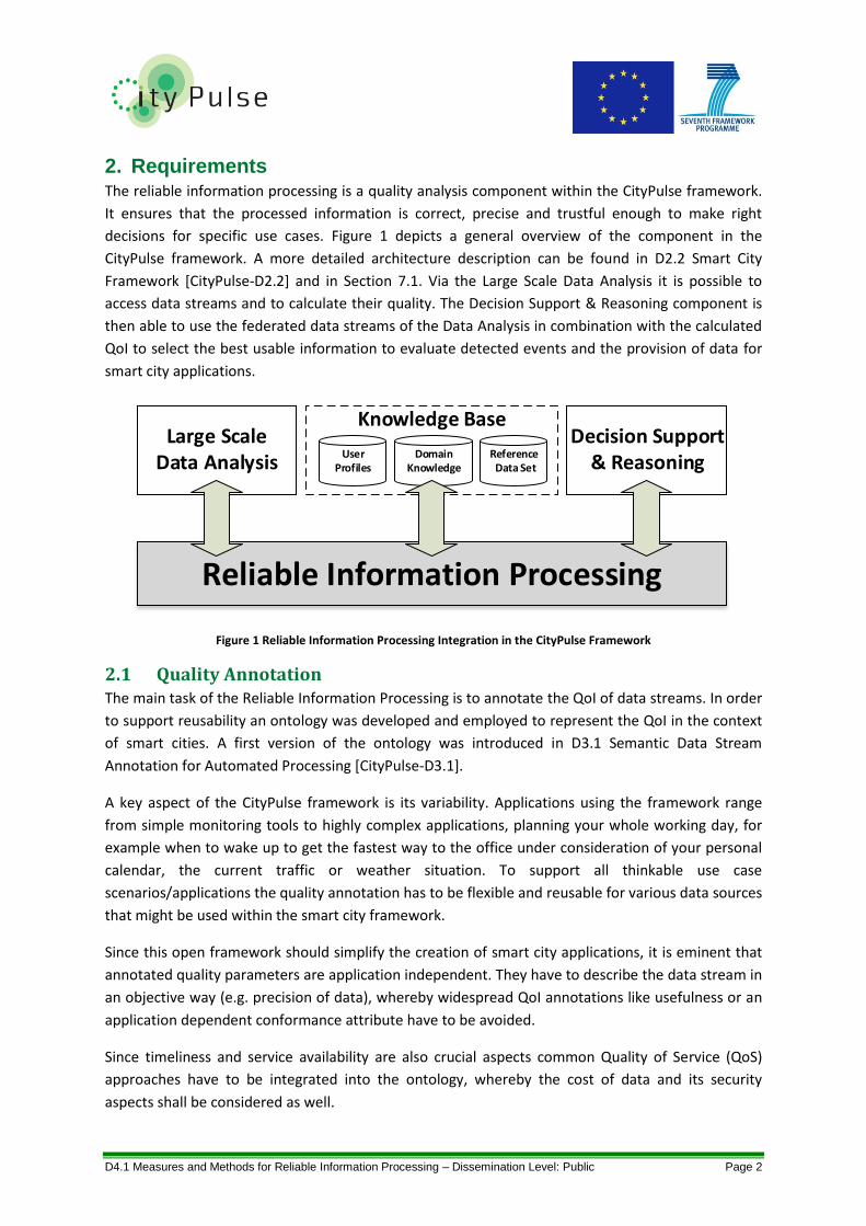
2. Requirements The reliable information processing is a quality analysis component within the CityPulse framework.
It ensures that the processed information is correct, precise and trustful enough to make right
decisions for specific use cases. Figure 1 depicts a general overview of the component in the
CityPulse framework. A more detailed architecture description can be found in D2.2 Smart City
Framework [CityPulse-D2.2] and in Section 7.1. Via the Large Scale Data Analysis it is possible to
access data streams and to calculate their quality. The Decision Support & Reasoning component is
then able to use the federated data streams of the Data Analysis in combination with the calculated
QoI to select the best usable information to evaluate detected events and the provision of data for
smart city applications.
Figure 1 Reliable Information Processing Integration in the CityPulse Framework
2.1 Quality Annotation The main task of the Reliable Information Processing is to annotate the QoI of data streams. In order
to support reusability an ontology was developed and employed to represent the QoI in the context
of smart cities. A first version of the ontology was introduced in D3.1 Semantic Data Stream
Annotation for Automated Processing [CityPulse-D3.1].
A key aspect of the CityPulse framework is its variability. Applications using the framework range
from simple monitoring tools to highly complex applications, planning your whole working day, for
example when to wake up to get the fastest way to the office under consideration of your personal
calendar, the current traffic or weather situation. To support all thinkable use case
scenarios/applications the quality annotation has to be flexible and reusable for various data sources
that might be used within the smart city framework.
Since this open framework should simplify the creation of smart city applications, it is eminent that
annotated quality parameters are application independent. They have to describe the data stream in
an objective way (e.g. precision of data), whereby widespread QoI annotations like usefulness or an
application dependent conformance attribute have to be avoided.
Since timeliness and service availability are also crucial aspects common Quality of Service (QoS)
approaches have to be integrated into the ontology, whereby the cost of data and its security
aspects shall be considered as well.
Large ScaleData Analysis
Reliable Information Processing
Decision Support& Reasoning
User Profiles
Domain Knowledge
Reference Data Set
Knowledge Base

D4.1 Measures and Methods for Reliable Information Processing – Dissemination Level: Public Page 3
2.2 Quality Analysis Automated rating of information quality for large number of data sources requires the development
of efficient algorithms to use QoI, availability, feedback information, etc. To use the results of the
analysis they have to provide quantifiable measures for rating the data sources and streams.
Methods to aggregate heterogeneous data sources with different accuracy, i.e. precision and
plausibility also have to consider the provenance and trustworthiness to compute the resulting
information quality. This enables smart city applications to retrieve information that fulfils the
requirements by finding the most suitable sources. Furthermore, it allows the identification and
exclusion of untrustworthy data sources to increase the reliability and operational robustness.
To adapt information quality approaches to the CityPulse framework, QoI and application
independent computation have to be realised. Therefore, the QoI parameters have to be expressive
and applied metrics must not hide information.
To obtain a scalable solution:
The analysis of single data streams has to be integrated in the virtualisation layer of the
information processing. By binding it close to the information source it gives the ability to
scale per stream.
Usage of incremental algorithms that do not need to recalculate all historical data, if new
datasets have to be integrated, have to be considered.
When suitable, use of predictive algorithms that are ready to give an accurate prediction
without the need to make all the calculation when receiving a query.
Training off-line, re-training only if necessary, re-train at time frames with low access/event
rates.
Announcement of changed/updated quality information via Publish/Subscribe.
Forget historical data out of scope.
Usage of light-weighted annotation.
The fault recovery component is triggered only when needed, for a short period of time and
it does not cache large amounts of stream data.
2.3 Conflict Resolution and Fault Recovery The main objective of the Conflict Resolution and Fault Recovery (CRFR) component is to increase
the stability of the system by providing alternative information sources when the quality of a stream
is modified (in most cases when the quality drops).
In reaction to the quality drop, the CRFR can identify an alternative stream to be used (feature
ensured by conflict resolution) or can generate estimated events using data from surrounding
sensors or historic data.

D4.1 Measures and Methods for Reliable Information Processing – Dissemination Level: Public Page 4
Conflict Resolution Requirements
Provide means to automatically derive soft/hard constraints using QoI descriptions from the
QoI data store.
Provide means to automatically convert the service composition request into hard and soft
constrains.
Use a constraints solver to obtain the solution.
From non-functional point of view: the service developer and the domain expert should use
this component without configuration or domain adaptation.
Fault Recovery Requirements
The component must be generic and the domain expert is the one who provides the
algorithm for providing solutions for emulating different streams data.
The algorithms for emulating different stream data have to be stored in the knowledge
database and the component must be able to identify/execute the model based on the fail
recovery requests.
Use interpolation methods and predictive algorithms to generate the estimation.
Inject estimated data in the same data streams where the measured data is transported; the
estimated events must contain a field, which states the fact that is an estimate.
Inject the emulated event when the real measurement (coming from the sensor) is missing
or when the current measurement or the trend (difference between two consecutive
measurements) is outside a specified range limit (set by the domain expert based on the
sensor capabilities, and the dynamics of the environment where it measures).
D4.1 Measures and Methods for Reliable Information Processing – Dissemination Level: Public Page 5
3. State of the Art In this section, we discuss the related work in the three main aspects of the deliverable, namely,
information quality annotation, information quality analysis, and conflict resolution & fault recovery.
3.1 Information Quality Annotation Data quality issues and faulty information are increasingly evident and have a high impact on
exploitation [Strong et al., 1997]. Strong et al.’s perspective is focused on the usage of large
organisational databases that contain data from multiple data sources. They mention other studies,
which assume that faulty, incorrect or incomplete data costs billions of dollars. To describe possible
issues affecting the usage of information they define four categories with a list of dimensions for
data quality. The categories are intrinsic, accessibility, contextual and representational. For each of
these categories the authors describe problem patterns to identify problems according to the data
quality. With the definition of categories and dimensions a basis for further investigation of data
quality is established. A framework for the assessment of information quality is presented by Stvilla
et al. in [Stvilia et al., 2007]. The framework is designed to be used as a general overview to develop
quality measurement models for specific settings. In contrast to other frameworks that are normally
planned to solve one local problem the framework’s parameters are more comprehensive.
Additionally the paper deals with possible problems that can occur when handling information
quality. A further development of application or context independent quality measurement is
described by Bisdikian et al in [Bisdikian et al., 2009]. To describe both application independent and
application dependent quality metrics they divide the quality into a Quality of Information (QoI) and
a Value of Information (VoI) part. A UML-based data model is introduced to support the splitting of
quality into the two parts and to provide a general template for future quality frameworks.
An often separately considered attribute for the description of a data stream is the provenance.
Provenance is the information about the origin of a data stream and therefore an indicator for the
trustworthiness of the provided data. In some works provenance is directly integrated into a QoI
framework [Bar-Noy et al., 2011], [Bisdikian et al., 2013]. Additionally an attribute called reputation
is used to describe the trustworthiness of data sources, as it is an aggregated value of single trust
values for information sources, which is mainly based on the past behaviour of the sources. In
[Ganeriwal et al., 2008] a reputation based framework is introduced to evaluate the trustworthiness
of sensor nodes. As every node needs a list of all neighbouring nodes this approach might not be
useful in the context of a smart city. Besides the fact that the calculations require additional
computation power, for different stream types (e.g. physical sensor and social media stream) the
approach cannot be realised on low-level sensors. The CityPulse framework needs a higher-level
approach where reputation is the ratio between the promised or expected quality value and the
measured one for all quality attributes. In summary for the CityPulse framework we need a quality
ontology that is adapted to a smart city environment and its dozens of possible different data
sources. Furthermore, the ontology needs to be application independent as possible future
applications using the framework are unknown, source oriented in kinds of consumption and costs,
and should contain a concept of handling trustworthiness.

D4.1 Measures and Methods for Reliable Information Processing – Dissemination Level: Public Page 6
3.2 Information Quality Analysis Smart cities are slowly adapting to the way of life of their inhabitants, which demand quick access to
answers and information for decision making in daily life activities; for example finding best
transportation choice to go to work, which could depend on information such as weather, traffic
conditions or polluted areas of the city. Providing this information involves processing a variety of
data coming from different sources with different QoI values. Dealing with QoI variations and
selecting the best possible information, always at the lowest system cost for each application, is a
challenging issue.
Smart cities use multi-modal information coming from heterogeneous sources including various
types of the Internet of Things data such as traffic, weather, pollution and noise data. The smart city
data usually has different QoI. QoI of each data source mainly depends on three factors: a) errors in
measurements or precision of the data collection devices; b) noise in the environment and quality of
data communication and processing (including network dependant QoS parameters, such as
throughput, latency, jitter, errors with drop or out of order packets or availability of the server); and
c) granularity of the observations and measurements in both spatial and temporal dimensions (i.e.
number of samples per unit of time and density of the data collection resources and their coverage
in an environment). Furthermore, various environments have different requirements that will
determine the efficacy of using the data in the smart city applications. Some systems have energy
restrictions due to battery power limitations and the energy cost of the wireless communications for
battery powered devices. Some wireless networks may rely on low bandwidth or intermittent
connectivity to Internet such as vehicular networks. Most of the smart city applications also have to
deal with huge volumes of data, high dynamicity of the data (this is especially important in scenarios
with mobile sensors), and a large variety of types of data including multimedia, text, and numerical
data.
The QoI issues become more challenging when various datasets with different QoI are integrated in
an application. In some of the current smart city frameworks the underlying information model is
based on semantic descriptions, which provide an annotation model to support interoperability
between different sources of information. These models can help to represent the QoI for each data
source; but the models and the annotated data are often represented as static descriptions, which
make them unsuitable for dynamic smart city data in which the quality can change over time. The
errors in measurements and communication, such as latency and noise and quality variations in
multiple sources, are some of these problems that make QoI issues more challenging in smart city
applications.
QoI in smart city frameworks is usually application dependent. Depending on the requirements the
solutions for enhancing the QoI could be different. For example, if the aim of an application is
seeking for trends in the data (i.e. traffic prediction based on historical data on weather, time and
events in the city) large samples could leverage the QoI. In this case, techniques for aggregation,
such as Symbolic Aggregate approXimation (SAX) algorithm [Kasetty et al., 2008], can help to create
a higher granularity representation of data by compressing data while keeping essential information.
Whereas, if the interest of the application is on latency and accuracy of the data, such as an

D4.1 Measures and Methods for Reliable Information Processing – Dissemination Level: Public Page 7
application that can return the number of free parking spaces in a city, the increase in the quality will
be determined by selection of trustable resources or a combination of data from multiple resources
to provide more accurate results.
The precision of the observations and measurements can be improved by increasing the frequency
and density of sampling and/or by using more accurate devices for sampling [Zhou et al., 2014]. In
order to reduce the effects of noisy environments, data pre-processing techniques can be applied to
reduce noise [Frenay & Verleysen, 2014]. In order to reduce the effect of the granularity of the
observations and measurements, different interpolation techniques such as linear, polynomial
interpolation and Gaussian models can be used [Mendez et al., 2013]. To overcome the volume
issues of the transmitted data in high frequency sampling, in-network fusion techniques or
dimensionality reduction techniques can be applied, which only transmit outliers [Brayner et al.,
2014]. The bandwidth limitation of the networks can be solved with similar techniques and also by
having a hierarchical storage, where most of the information can be stored in the source device but
less information is transmitted to the applications, using sampling or other aggregation techniques.
When more granularity of the data is requested the source could be accessed and when less
granularity is requested the sampled or aggregated data could be accessed.
Most of the data aggregation and interpolation solutions assume that the QoI at the origin of the
data is higher than the application level. However, if information is created by combining multiple
data, the accuracy of the processed information can be higher than the original data at individual
sources. In order to keep track of the information processing it is necessary to annotate the
provenance of the information [Kolozali et al., 2014].
In order to describe and use the quality related parameters of the smart city data we propose using
lightweight dynamic semantics [Barnaghi, 2014]. The semantic models will provide interoperable
descriptions of data and their quality and provenance attributes. The semantic annotation of quality
parameters is useful for interoperability and knowledge based information fusion. In order to make
semantics scenario independent and to be able to fast annotate and process ontologies we propose
lightweight semantic models, which contain only a few general concepts, without many reasoning
rules. Data processing software can then update the QoI in these models. As the data quality
parameters of the data sources are updated, these changes can then be linked to and reflected in
their semantic descriptions. So the processing applications can access the semantic description to
determine the quality parameters of the data descriptions.
For the aggregated and complex data that is integrated from multiple sources, the provenance
parameters can help to trace the QoI parameters of each source and quality aspects of the
processing algorithms and methods that are applied to the data. However, updating the dynamic
semantic models and determining the quality of data at the sources, quality of the network and
environment and also the processing components and monitoring their changes over different
time/location dimensions is still a key challenge.
Overall smart city data relies on large-scale deployment of multi-vendor, multi-provider devices,
networks and resources that usually operate in noisy and dynamic environments. The temporal and
D4.1 Measures and Methods for Reliable Information Processing – Dissemination Level: Public Page 8
spatial density of sampling of data collection will have an impact on the quality of the smart city
data. Different environment and network parameters add limitations such as latency and noise.
Energy constraints will also have an impact on the quality of data. Semantic descriptions and
annotations can be used to describe different features of the smart city data and their quality
attributes. However, the conventional semantics are usually static and their complexity hinders their
application in very large-scale deployments and (near) real-time applications. We propose using
lightweight semantic models with provenance information and combining semantics with data
interpolation and data analytic models to create dynamic semantic description of quality parameters
in a smart city framework.
Our work for this deliverable was to apply novel data analytic techniques in the field of smart cities,
to enhance the quality of information, while annotating the QoI parameters of each data stream,
and keeping it up to date in a triple-store. Some of the novel techniques we apply enhance the
precision of the sources including new correlation techniques not being used before in smart cities.
The analysis of smart cities is an emerging field of research and only a few works have analysed the
correlations between different sensors in the context of cities (e.g. [Lathia et al., 2012], [Quercia et
al., 2012]). All these works have utilised Pearson correlations in the analysis. However, it is well
known that Pearson correlation has some drawbacks. Pearson correlation fails to detect the
dependency between two or more variables, when the data has some specific distributions, such as
non-linear distributions. In the field of statistics some alternatives are available, such as distance
correlation, mutual information or correlation ratio. Although none of them are completely
accurate, these alternatives could give a better hint of the dependency of data or could complement
the Pearson correlation. We have used different of these techniques, such as mutual information,
reward and punishment, and conformance analysis of affecting streams (see Section 5). In order to
reduce the noise in sources, especially the missing values, and the granularity of the sources, we
have applied interpolation techniques with the use of dynamic semantics to reduce the annotation
processing (see Section 5.5.)
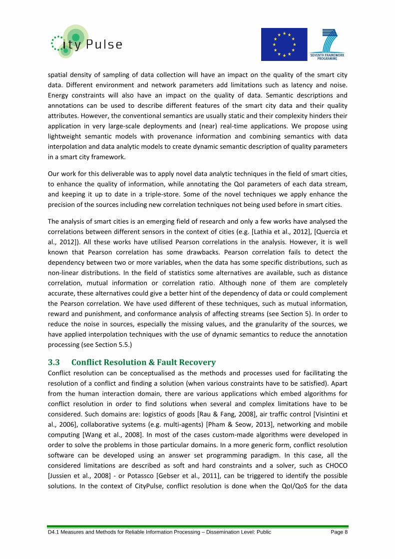
3.3 Conflict Resolution & Fault Recovery Conflict resolution can be conceptualised as the methods and processes used for facilitating the
resolution of a conflict and finding a solution (when various constraints have to be satisfied). Apart
from the human interaction domain, there are various applications which embed algorithms for
conflict resolution in order to find solutions when several and complex limitations have to be
considered. Such domains are: logistics of goods [Rau & Fang, 2008], air traffic control [Visintini et
al., 2006], collaborative systems (e.g. multi-agents) [Pham & Seow, 2013], networking and mobile
computing [Wang et al., 2008]. In most of the cases custom-made algorithms were developed in
order to solve the problems in those particular domains. In a more generic form, conflict resolution
software can be developed using an answer set programming paradigm. In this case, all the
considered limitations are described as soft and hard constraints and a solver, such as CHOCO
[Jussien et al., 2008] - or Potassco [Gebser et al., 2011], can be triggered to identify the possible
solutions. In the context of CityPulse, conflict resolution is done when the QoI/QoS for the data

D4.1 Measures and Methods for Reliable Information Processing – Dissemination Level: Public Page 9
streams used by the applications drops. In that case an alternative data source has to be identified
based on the application request, which contains the types of the data and sufficient QoI/QoS.
The fault recovery is the property that enables the system to recover in the event of failure and to
continue the operation properly. There are no standard recovery methodologies that can be applied,
and the algorithms are implemented based on the possible failure directions. In case of CityPulse
framework, the fault recovery will allow the application to continue the operation even if the
QoI/QoS of the streams drops. This is archived by generating estimated events, using Machine
Learning (ML) or interpolation models.
Machine Learning evolved as a major branch of Artificial Intelligence. This paradigm targets
development of algorithms, which are able to improve their behaviour based on the acquired
experience. The models resulted in ML are mainly data driven, although a ML expert is critically
involved in deciding which type of ML algorithm is the most appropriate for given task and data.
Among the predictive analytics applications, which benefit by the ML advances, also applicable for
the predictive manufacturing, one can identify various classes of scenarios: automatically building
models to detect anomalies/outliers in a data stream; time series forecasting (predicting values that
are supplied when a specific sensor temporarily stops to deliver data); predicting classes or
continuous output values which are most likely to be associated to current input values (based on
the model learned so far); learning associations between values and producing association rules;
automatic feature extraction and feature learning (which mostly used as pre-processing
mechanisms); uncertainty management (through the most classical approaches: probabilistic models
and fuzzy systems, which offer support for various types of uncertainties).
The available learning methodologies are considerable and are to be chosen based on the
application. Some of the commonly employed machine learning algorithms include: artificial neural
networks [Haykin, 1998], Support Vector Machines [Scholkopf & Smola, 2002], Bayesian networks
[Koller & Friedman, 2009], decision trees, association rule learning, and clustering algorithms (these
are only a small part of classical methods of ML). We also witness an upsurge interest in ensemble
methods, i.e. combining multiple learners [Seni & Elder, 2010].
The ML models are very versatile and can be used for generating estimated data based on the
historic data acquired from that specific source. In other words the model does not rely on other
similar data sources from the proximity. In the case the stream quality drops for a longer period it is
highly probable that the prediction quality will decrease. But there are situations when one can use
data sources from the proximity if the sensor has failed. In this specific case interpolation methods
can be applied such as: Kriging or Spline [Knott, 2000].
D4.1 Measures and Methods for Reliable Information Processing – Dissemination Level: Public Page 10
4. Quality Metrics for Reliable Information Processing This section details the annotation of sensory data with semantic descriptions specifying information
quality. It introduces an application independent approach for defining QoS and QoI of data streams
using an ontology and machine interpretable language (i.e. RDF). Furthermore, a model for the
consideration of provenance and trustworthiness is presented.
4.1 Data Stream Quality Definition In a smart city environment many different data sources can be found. They can be grouped by their
complexity and their provided data types. On the one hand there are primitive sensors, which
measure simple physical values, for example temperature sensors or traffic sensors that are
counting a number of cars, which have passed by the sensor. On the other hand more complex data
sources exist. An extensive example would be the usage of social media streams and the extraction
of events from the stream (e.g. extracting traffic information from a Twitter stream) or a web
interface, which provides live timetables for the departure of buses within the city. In addition the
data sources may differ in their dynamic nature (e.g. the static printed timetable at a bus station
compared to a live updated electronic display). A smart city consists of dozens of different data
sources. Some of them might overlap, whereas others might be exclusive. To ensure a reliable
processing of the information these data sources provide the data, which has to be validated within
the smart city framework. Due to the different data sources and various use cases for smart city
applications it is not feasible to determine the QoI with respect to the application’s requirements.
Therefore the reliable information processing of the CityPulse framework uses an application
independent approach.
To ensure the application independence an ontology describing the quality of data sources is
developed. The ontology contains a list of different quality parameters that are used by other quality
ontologies known from literature. As some parameters are defined differently in the literature they
were redefined. To avoid confusion regarding the parameters, Table 1 lists the parameter names
with their belonging definition as they are used for the CityPulse quality ontology. The table itself is
divided into categories. The Accuracy and the Timeliness categories contain attributes to describe
the information quality, whereas the Communication category describes typical Quality of Service
attributes. Additionally the Cost and Security categories provide static information about a data
source regarding costs for the usage or attributes on how it might be encrypted or published.
To calculate the quality of a data stream, it is important to know some information about the data
source. For example it is nearly impossible to extract information about the costs of a stream from
raw data. Thus some stream parameters, especially for the Cost and Security category, have to be
annotated during a stream registration phase. In addition the other parameters should be annotated
with the expected stream values too. For example the parameter Frequency will be compared with
the initial annotated stream frequency to determine the quality of the data stream. The list below
describes the five main categories of the information quality:

D4.1 Measures and Methods for Reliable Information Processing – Dissemination Level: Public Page 11
Accuracy: The parameters in the Accuracy category are used to describe the degree to which
delivered information is correct, precise and complete. The registration of expected values
for the data stream resolution and deviation, as well as the comparison with geo-spatial
related sensors enables the CityPulse quality system to determine the Correctness and
Completeness.
Communication: As stated the Communication category contains attributes related to
typical QoS requirements of a data stream. With this category it is possible that an
application receives only information from data sources that fulfil a specified QoS demand
e.g. have only a small packet loss.
Cost: The Cost category enables the quality ontology to describe the monetary, energy and
network costs of a data stream. This allows an application (depending on the user’s
preferences) specify which data sources the CityPulse framework should select to get the
most cost-efficient data source.
Security: This category contains parameters to describe the permission-levels for provided
data, e.g. if the data owner allows to republish/distribute the data or prohibits any further
usage. Furthermore parameters to describe the encryption and data integrity through
signing mechanisms are stated here.
Timeliness: The Timeliness category allows choosing data streams by their update
frequency, the amount of time information is valid, the timespan between the data
measurements and the publication time.
Table 1 shows a complete view of all quality categories with their sub-attributes. In addition, the
range for possible values and an example are added. For instance the resolution is annotated in a
range of (0, ∞). The example indicates that values of the annotated sensor data stream have a
resolution of 0.1°𝐶, which is not as accurate as a sensor with a degree of 0.001°𝐶 would be. A
different annotation is the description of the monetary consumption that indicates the monetary
cost a stream has for its usage. It ranges from 0 to infinite. Another example is a cost of 0.03€ per
request. However the sub-attribute frequency of the timeliness category specifies how often a
stream sends an update. It is annotated with a value range from 0 to infinite. The example of 60s
indicates that an update could be expected every minute. The annotated quality values are used for
the process of quality calculation as it is described in detail in Section 5.3.

D4.1 Measures and Methods for Reliable Information Processing – Dissemination Level: Public Page 12
Table 1 Quality Parameter Definitions
Figure 2 depicts a simplified version of the Quality Ontology (prefixed qoi) without the subcategories
of quality attributes. As a connection to the to the CityPulse information model parts of the Stream
Annotation Ontology (SAO) are integrated. In addition the provenance aspects are realised with the
usage of the PROV-Ontology (PROV-O). To annotate a data stream with quality information a
qoi:hasQuality relation is introduced. Via this relation every soa:StreamData or soa:Segment gets a
defined QoI.
subcategory Measurement unit Range Example
Probability that information is within the range of precision and
completeness[0,1] 0.88
Resolution Resolution detail for the measured value. (0,∞) 0.1°C
Deviation (max) The maximum percentage of deviation from the real value. [0,1] +-0.1
The ratio of attribute values compared to expected parameters. [0,1] 0.97
Packet LossThe probability that a set of data / a packet will not be transported
correctly from the source to its sink.[0,1] 1/10^6
BandwithMin/Avrg/Max amount of bandwidth that is required to transport
the stream.(0,∞) 100bps
LatencyMeasurement of the time delay between the stream is sent and
received in the virtualisation layer.(0,∞) 30ms
Jitter Deviation from true periodicity of an assumed periodic signal. (0,∞)10ms or
2500ms
Throughput
The amount of useful information sent by the network (ex: sensor
data), taking out the headers and protocol information sent in the
network.
(0,∞) 100bps
Queuing Type Type of queuing, e.g. FIFO, LIFO, unordered.FIFO|LIFO|
unordered|...FIFO
Ordered Probability that datasets arrive in the defined order. [0,1] 0.92
The amount of energy used to access the steam. (0,∞) 1W
Is the usage of the stream free of charge or how much does it cost. [0,∞)0.03€/
requests
How much traffic is caused by usage of the data source. (0-∞) 10bps
licence defintionReference to Licence class, e.g.
http://creativecommons.org/ns#Licence.reference -
may be used…Reference to Permission class, e.g.
http://creativecommons.org/ns#Permission.reference -
may be publishedReference to Permission class, e.g.
http://creativecommons.org/ns#Permission.reference -
Encryption method, authority for key management.as defined in
RFC4253 p. 9aes256-cbc
authority Certificate authority. text cacert.org
public key Key to decrypt signatures. binary -
The time an information was created/measured/sensed. (0,∞) 180s
Maximum timespan between two datasets. (0,∞) 3600s
The amount of time the information remains valid in the context of
a particular activity.(0,∞) 60s
Cost
Parameter-name
Accuracy
Correctness
Precision
Completeness
Communication
Network Performance
Queuing
Energy Consumption
Monetary Consumption
Network Consumption
Security
Timeliness
Age
Volatility
Frequency
Confidentiality (reuse of rights ontology, e.g. http://creativecommons.org/ns)
Encryption
Signing

D4.1 Measures and Methods for Reliable Information Processing – Dissemination Level: Public Page 13
Within the SAO the PROV-O is embodied to build a relation with the prov:used connection between
a sao:StreamEvent and a sao:StreamData. The PROV-O is reused for the Quality Ontology to
integrate a concept of provenance. To add provenance information, the sao:StreamData needs to be
subclassed from prov:Entity. The prov:Entity has an origin which is indicated by a
prov:hasProvenance relation to a prov:Agent, which is the owner of the data stream. An prov:Agent
is defined as an organisation, a person or a software agent. To define the trustworthiness of a data
source the class qoi:Reputation, which is defined within the quality ontology, is used. The concept of
reputation allows reflecting the experience by applications while using the data source and is subject
to further research. Main idea for the usage of the reputation concept is that every data source has
an owner (prov:Agent) which gets assigned a reputation. This reputation is calculated based on the
previous behaviour and mainly influenced by the provisioning of wrong/faulty data.
Figure 2 Quality Ontology
4.2 Annotating Data Stream Quality With the Quality Ontology it is possible to annotate the quality of data streams. The Terse RDF Triple
Language (Turtle) data format has been used for the annotation. Turtle is used to describe datasets
within RDF data models. It is an alternative to the XML representation of RDF files and makes files
compact and easy to read. As well as in XML-RDF the Turtle format presents information in form of
triples. Each triple contains a subject, a predicate and an object to describe data elements and its
relations.
The defined quality ontology from chapter 4.1 is implemented using the ontology editor protégé
which creates an OWL file with the ontology description. One view of the editor with the class
hierarchy of the ontology and the definitions of the quality classes is depicted in Figure 3.

D4.1 Measures and Methods for Reliable Information Processing – Dissemination Level: Public Page 14
Figure 3 Quality Ontology in Protègè
1 @prefix : <http://ict-citypulse.eu/experiments/Experiment1/> .
2 @prefix prov: <http://purl.org/NET/provenance.owl#> .
3 @prefix qoi: <http://ict-citypulse.eu/ontologies/StreamQoI/> .
4 @prefix rdf: <http://www.w3.org/1999/02/22-rdf-syntax-ns#> .
5 @prefix rdfs: <http://www.w3.org/2000/01/rdf-schema#> .
6 @prefix sao: <http://purl.oclc.org/NET/UNIS/sao/sao> .
7 @prefix ssn: <http://purl.oclc.org/NET/ssnx/ssn#> .
8 @prefix tl: <http://purl.org/NET/c4dm/timeline.owl#> .
9 @prefix xml: <http://www.w3.org/XML/1998/namespace> .
10 @prefix xsd: <http://www.w3.org/2001/XMLSchema#> . 11 12 :segment-sample-1 a sao:Segment ; 13 qoi:hasQuality : 14 :completeness-sample-1, 15 :correctness-sample-1, 16 :frequency-sample-1 ; 17 ssn:observationResultTime [ a tl:Interval ; 18 tl:at "2014-08-01T09:00:00"^^xsd:dateTime ; 19 tl:duration "PT00H05M"^^xsd:duration ] ; 20 prov:hasProvenance :R_ID158355 . 21 22 :completeness-sample-1 a qoi:Completeness ; 23 qoi:value "1.0"^^xsd:float . 24 25 :correctness-sample-1 a qoi:Correctness ; 26 qoi:value "0.99"^^xsd:float . 27 28 :frequency-sample-1 a qoi:Frequency ; 29 qoi:value "1.0"^^xsd:float . 30 31 R_ID158355 a prov:SoftwareAgent .
Listing 1 Quality Annotation
Listing 1 depicts an annotated example of a traffic stream from ODAA (see section 5.2). In the first
ten lines the ontologies are included (e.g. the StreamQoI ontology in line 3 or the Stream Annotation
ontology in line 6) to describe the dataset. Starting with line 12 the dataset is described with the
mentioned RDF-triples. The segment-sample-1 is defined as a Segment of the SAO ontology, which
has some related quality attributes with a qoi:hasQuality property from the StreamQoI ontology. An
example for a complete triple within the listing is segment-sample-1 qoi:hasQuality Completeness.

D4.1 Measures and Methods for Reliable Information Processing – Dissemination Level: Public Page 15
Concrete values for the calculated quality within the linked attributes are annotated in the example
(e.g. line 25/26: a Correctness of 0.99). In addition to the quality the provenance of the data
segment is annotated. With the prov:hasProvenance property of the PROV-O ontology it is assigned
to a prov:SoftwareAgent in line 31.
4.3 Influence of Provenance In addition to the QoI model the CityPulse framework uses a concept of provenance and reputation
to provide a factor of trustworthiness for data streams. The Quality Ontology, introduced in Section
4.2, enables the framework to annotate an owner for every data source. This owner is the
provenance of a data stream, which can be a person, an organisation or a software agent. Each
owner gets a profile including a static reputation value.
Person: A person normally starts with a low reputation value as a person experiences only a
individual view of information. As an outcome the possibility that a person provides
inadvertently or intentionally faulty information is higher than the probability that an
organisation, e.g. the public transport company, delivers false information.
Organisation: An organisation represents the opinion of more than one person. In contrast
so a single person as the owner of a data stream often a team of company workers or
automated systems are responsible for the provided information. Due to these facts, it is not
impossible that an organisation provides faulty information within their data streams but is
less probable than a stream owned by a single person.
Software agent: A software agent is a running software which processes data streams. As
the running software might be supported by machine learning algorithms it cannot always
be assigned to a person or an organisation running the software. For this reason a software
agent gets his own reputation.
Figure 4 Reputation Use Case

D4.1 Measures and Methods for Reliable Information Processing – Dissemination Level: Public Page 16
To demonstrate the concept of reputation, Figure 4 depicts an example use case in a public
transport scenario. The figure shows people that are using a smart travel application on their mobile
phones. At one bus stop a person is watching an accident involving the bus he is waiting for. As it is
probable that the bus has a delay or might be cancelled, he informs other people by reporting the
accident to the smartphone application. Via the smart application the people, which are waiting for
the crashed bus, are now informed and can possibly take another bus to their destination instead of
waiting for the bus that should be in time, as the electronic display of the public transport company
at the bus stop reports.
Until now, there is no integration of reputation or trust in the scenario, but what might happen if a
user misuses the smart application and reports a delayed or cancelled bus as nothing happened? The
application will falsely inform other people about the delay. To avoid a misuse, the reputation is
included. In a first step two involved agents are annotated with a reputation:
Person: every person using the smart application gets a value of 0.2 (range from 0 to 1) for
their reputation.
Public transport company: the company gets a value of 0.5 for its reputation value as their
buses a normally in time or delays a reported correctly.
With the usage of reputation the use case progress is a bit different. If there is only a single person
reporting the possible delay of the bus and the public transport company reports that the bus is in
time, the smart application respectively the CityPulse framework decides that there is no delay
because the reputation of the company is higher than the reputation of one single person. A
different decision is made if more than one person reports a delayed bus. If for example three
persons report the delay, the sum of their reputation might be higher as the one of the public
transport company.
For the summarisation of individual reputation values there are some additional aspects that should
be included to weight the reputation values. As the authors in [Emaldi et al., 2013] describe, it is
advisable to include factors like timeliness or distance to summarise the reputation. The distance
weight is calculated as follows:
𝑡𝑟𝑢𝑠𝑡𝑑𝑖𝑠𝑡𝑎𝑛𝑐𝑒 =1
𝑔𝑒𝑜𝑑𝑖𝑠𝑡𝑎𝑛𝑐𝑒(𝑙𝑜𝑐𝑟𝑒𝑝𝑜𝑟𝑡 , 𝑙𝑜𝑐𝑟𝑒𝑝𝑜𝑟𝑡𝑒𝑑𝑝𝑙𝑎𝑐𝑒)
The formula calculates a factor based on the distance between the person that reports a possible
delay and the position of the reported event. If a person reports information, which is far away from
his current position, it is weighted lesser than reports by persons nearby. The same method is used
for the temporal distance. If an event is reported shortly after its occurrence it is weighted higher.

D4.1 Measures and Methods for Reliable Information Processing – Dissemination Level: Public Page 17
5. Methods for Reliable Information Processing This section describes methods for the determination of quality parameters based on the analysis of
data streams. Based on the available datasets different approaches are envisaged by experimental
results on a reference dataset. To actively provide information quality an approach for the utilisation
of dynamic semantics is explained.
5.1 Utilisation of Available Information A vast number of heterogeneous interfaces and data formats have to be adapted to use the full
variety of information sources in city deployments. Furthermore, the varying information quality and
uncertain reliability of multiple information providers has to be considered in the selection of the
best available data stream. Therefore, CityPulse continuously monitors and calculates the
information quality of incoming data streams and exploits this meta-information to provide reliable
applications.
Based on the available information, there are several different calculation approaches to determine
the Correctness quality of a stream. If spatial related sensors can be found, their readings can be
compared to determine their Correctness. While it may be adequate to compare an observation of a
pollution sensor to the nearest sensor, it is necessary to involve the exact position of a traffic sensor
within the road system, as the nearest sensor may be on a different street, which is possibly not
related to the origin sensor.
The second approach deals with the usage of multiple information sources. An example may be the
comparison of ODAA (see section below) and Here Traffic information provided by Nokia. Relations
between different sensors/data streams with different types have to be found in contrast to the
single information source approach. If it is possible to find spatial related data sources, which are
measuring the same feature, the next step is to compare their provided information taking into
account the attributes of the data streams, such as resolution or scale of the underlying sensor.
Furthermore the combination of streams with different features is possible. An example for the
composition of sensors with different attributes can be given as an average speed on a street
measured by a sensor and the total number of cars measured by another sensor. Figure 5 shows
different categories for the calculation based on the used information sources.
D4.1 Measures and Methods for Reliable Information Processing – Dissemination Level: Public Page 18
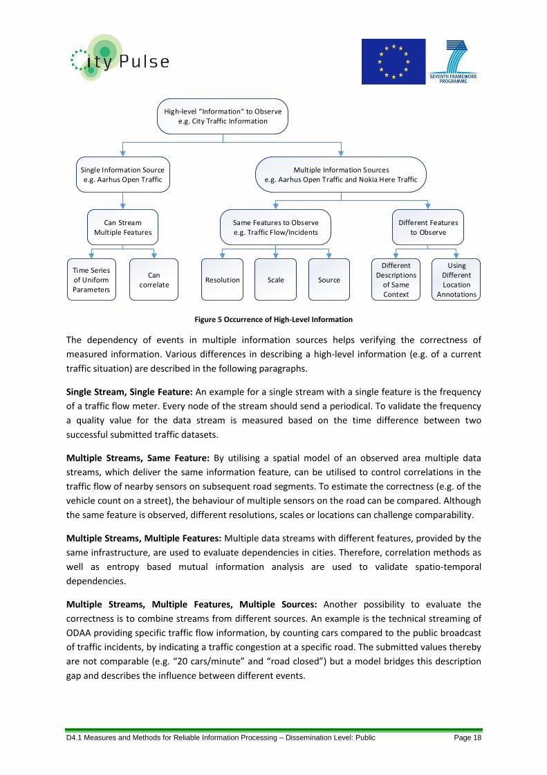
Figure 5 Occurrence of High-Level Information
The dependency of events in multiple information sources helps verifying the correctness of
measured information. Various differences in describing a high-level information (e.g. of a current
traffic situation) are described in the following paragraphs.
Single Stream, Single Feature: An example for a single stream with a single feature is the frequency
of a traffic flow meter. Every node of the stream should send a periodical. To validate the frequency
a quality value for the data stream is measured based on the time difference between two
successful submitted traffic datasets.
Multiple Streams, Same Feature: By utilising a spatial model of an observed area multiple data
streams, which deliver the same information feature, can be utilised to control correlations in the
traffic flow of nearby sensors on subsequent road segments. To estimate the correctness (e.g. of the
vehicle count on a street), the behaviour of multiple sensors on the road can be compared. Although
the same feature is observed, different resolutions, scales or locations can challenge comparability.
Multiple Streams, Multiple Features: Multiple data streams with different features, provided by the
same infrastructure, are used to evaluate dependencies in cities. Therefore, correlation methods as
well as entropy based mutual information analysis are used to validate spatio-temporal
dependencies.
Multiple Streams, Multiple Features, Multiple Sources: Another possibility to evaluate the
correctness is to combine streams from different sources. An example is the technical streaming of
ODAA providing specific traffic flow information, by counting cars compared to the public broadcast
of traffic incidents, by indicating a traffic congestion at a specific road. The submitted values thereby
are not comparable (e.g. “20 cars/minute” and “road closed”) but a model bridges this description
gap and describes the influence between different events.
High-level “Information“ to Observee.g. City Traffic Information
Single Information Sourcee.g. Aarhus Open Traffic
Multiple Information Sourcese.g. Aarhus Open Traffic and Nokia Here Traffic
Can Stream Multiple Features
Same Features to Observee.g. Traffic Flow/Incidents
Different Features to Observe
Time Series of Uniform Parameters
Can correlate
Resolution Scale Source
Different Descriptions
of Same Context
Using Different Location
Annotations
D4.1 Measures and Methods for Reliable Information Processing – Dissemination Level: Public Page 19
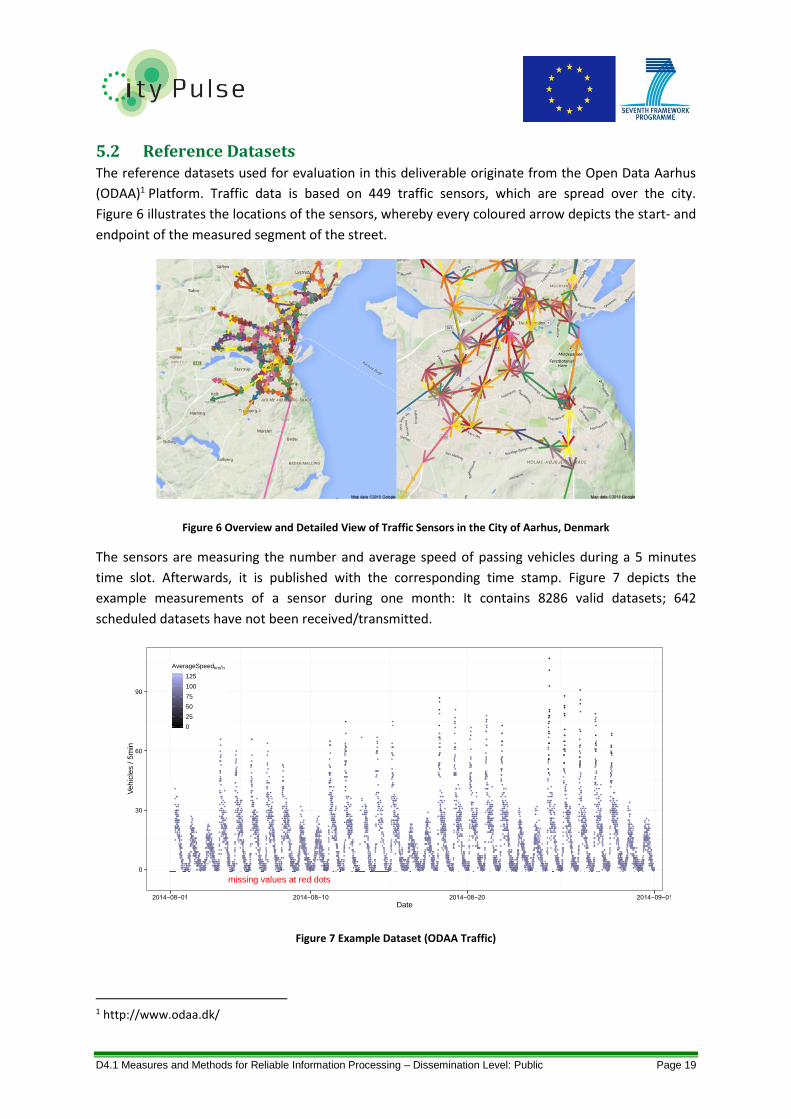
5.2 Reference Datasets The reference datasets used for evaluation in this deliverable originate from the Open Data Aarhus
(ODAA)1 Platform. Traffic data is based on 449 traffic sensors, which are spread over the city.
Figure 6 illustrates the locations of the sensors, whereby every coloured arrow depicts the start- and
endpoint of the measured segment of the street.
Figure 6 Overview and Detailed View of Traffic Sensors in the City of Aarhus, Denmark
The sensors are measuring the number and average speed of passing vehicles during a 5 minutes
time slot. Afterwards, it is published with the corresponding time stamp. Figure 7 depicts the
example measurements of a sensor during one month: It contains 8286 valid datasets; 642
scheduled datasets have not been received/transmitted.
Figure 7 Example Dataset (ODAA Traffic)
1 http://www.odaa.dk/
●
●
●
●
●
●
●
●●●●●
●
●
●
●●
●●●
●
●
●
●●
●●
●
●
●
●
●●●
●
●
●●
●●
●
●●
●●●●
●●●
●
●
●
●
●
●
●●
●
●
●
●
●
●
●●
●
●●
●
●
●●
●
●
●
●●
●
●●●●
●
●
●
●
●●●
●●
●●●●
●●●
●●
●●●●●●●●●●
●●●●●
●●
●
●●●
●●
●●
●●●●●●●
●●●●
●●●●
●●●●●●●●●●●●●●●●●●●
●●●●●●●●●●●●●●●●●●●●●●●●●●●●●●●●●●●●●●●●●
●●●●●●
●●
●
●●
●●
●●●
●
●
●
●●
●
●
●
●
●●
●
●
●●
●●
●
●●
●
●
●●
●
●
●
●
●
●●●●●
●
●
●●●
●
●●●●●
●
●●
●
●●
●●
●
●
●
●●
●●
●
●
●
●●●
●
●●
●
●
●
●●●
●●●●
●
●●●●
●
●
●
●●
●●
●
●
●●
●●
●
●
●●
●●
●
●●
●●●
●●●●●●
●
●
●●
●●
●
●
●●
●
●
●●
●●●
●●
●●●●●●●●●●●●
●
●●
●●●●●●●●●●●●●
●●●●●●●●●●●●
●
●●
●●●
●●
●●
●●
●●●
●
●●
●●●●●●●
●
●●●●●●●●●●●●●●●●●●●●●●●●●●●●●●●●●●●●●●●●●●●●●●●●●●
●●
●●●●●●●●●●●●●
●●
●●●●●●
●●●●●
●●
●●●●●●
●●●●●●●
●●●●●●●
●●●
●●●●
●●●
●
●
●●
●
●●●●
●●●
●●
●
●●●●●
●
●
●
●
●
●
●
●
●●
●
●
●●
●●
●●
●
●
●●●●●
●●
●●
●●
●
●●
●●
●●
●
●
●
●
●
●
●●●
●●
●●●
●●●
●●
●●
●
●
●
●
●
●●
●●●●●●●●
●
●●●●
●
●●
●●
●●
●
●●●
●
●●
●●
●
●●●●●
●●●
●●
●●
●●
●●
●●●
●●●●●●●
●●●●●
●●●●
●●●●●●●●●●●●●●●●●●●●
●
●●●●●●●●
●●●●●●●●●●●●●●●
●●●●●●●●●●●●
●●●●●●●●●●●●●
●●●●●●
●●●●
●●●
●●
●
●●
●
●
●
●
●
●
●●
●
●
●
●
●
●●
●
●
●
●
●
●
●
●●
●
●
●
●
●
●●
●
●
●
●●
●●
●●
●●
●●
●●●●
●●
●●
●
●
●●
●
●●
●●
●●
●
●
●
●●
●
●
●
●
●
●
●●
●●
●
●●
●
●●●
●
●●●
●●
●●
●
●
●
●
●●●●
●
●
●
●●●
●
●
●
●●
●●
●
●●
●●
●
●●
●
●●●●
●●
●
●
●●●
●●●●●●●
●●●
●
●
●
●
●
●●
●
●●
●
●
●
●●●●●●●
●●●●●●●
●●●●●●●
●●●
●●●●●●●
●
●●●●●●●●●●●●●●●●●●●●●●●●●●●●●
●●
●●●●●●●●●●●●●●●●●●
●●●
●
●●●
●●●●●●●●●●●●
●
●●
●●●
●
●
●
●
●
●●
●
●
●
●
●
●
●
●
●
●
●
●
●
●
●
●●
●●
●
●
●
●
●
●
●
●●●
●
●
●
●●
●●●
●
●
●
●
●
●
●
●●
●
●●
●
●
●
●
●
●●●●
●●
●
●
●
●
●
●●
●
●
●●
●
●●
●
●●
●
●
●
●
●
●●
●
●
●
●
●●●
●●
●
●
●
●
●
●
●
●
●
●
●
●
●●
●
●●
●
●●
●●
●
●●
●
●
●
●●
●●
●●●
●
●
●●●●
●●
●
●●
●●
●
●
●●●
●●●●●●●●●●●●
●●●
●
●
●●
●●
●●●
●
●●
●
●
●●
●●●●●●●
●●
●●●●●●●●●●●●●●
●
●●●●●●●●●●●●●●●●●●●●●●●●●●●●●●●●●●●●
●
●●●
●
●
●●●●
●
●
●●●●
●●
●
●
●
●
●
●
●
●●
●
●
●
●
●
●
●●●
●
●●
●
●
●
●
●
●
●
●
●
●
●
●
●
●
●
●●
●
●
●●
●●
●
●
●
●
●●●
●
●
●
●
●
●●●
●●
●
●
●
●●●●●●●
●
●
●●●
●●
●
●
●
●
●●
●
●●●
●●●●●●●
●
●●
●
●
●●
●
●
●
●
●
●
●
●
●
●
●
●●
●●
●
●
●
●
●
●
●
●●●
●
●
●●
●
●
●
●●●●
●
●
●●●●
●
●●
●
●
●●
●
●
●●●
●●●●
●
●
●●
●●
●●●●
●●
●●●●
●●●●●●●
●●
●●●●●
●●●●
●●●●●
●
●●●●●●●●●●●●
●
●●●●●
●●●●●●●●●●●●●
●●●●●●●●●●●●●●●●●●●●●●●
●●
●●●●
●
●
●
●●●
●●●
●●
●
●
●
●
●
●
●
●●
●●
●
●
●
●
●
●
●●
●
●
●
●
●●
●
●
●
●
●
●●●
●
●
●
●●
●●●
●
●
●
●
●
●
●
●
●
●
●
●
●
●
●●●
●
●
●●
●
●
●
●●
●
●
●
●
●
●
●
●
●
●●
●
●
●
●
●
●●
●●●
●●
●
●
●●
●●●
●
●
●
●
●●
●
●
●
●
●
●●
●●●●●
●
●●
●
●●●
●●
●
●
●
●●●●●●●
●
●
●
●
●
●
●●●
●
●
●●
●●●
●
●
●●●●
●●
●●●●●
●●
●●
●●●●●●●
●●●●
●●●
●●●●●
●●●●●●
●●
●
●
●●●●
●●●●●
●●
●●●●●
●●●●●●●●●●●●●●●●●
●
●●●●●●●●●●●●●●●●●●●●●
●●
●●●
●
●●●
●●
●●
●
●
●
●
●
●
●
●●●
●
●
●
●
●
●●
●●
●●
●
●
●
●
●
●
●
●
●
●
●
●
●
●
●●●
●●
●●
●
●
●
●
●
●
●●●
●●●
●
●
●
●●
●
●
●●●
●
●
●●
●●
●●
●●●
●
●
●
●
●
●●●●
●
●●
●
●
●
●
●●
●
●
●
●
●
●
●●●
●
●
●
●
●●
●●
●●●●
●
●
●●
●
●
●●
●●●
●
●
●
●
●
●
●●
●
●
●●
●
●●
●●●●●●
●
●
●●●
●
●
●●
●
●●●●●●●●●●
●●
●●●●●●●●●
●
●
●
●
●●
●●●
●
●●●●●●●●●●●●●●●●●
●●●●●
●●●●●●
●
●●●●●●●●●
●
●●●●
●●●●●●●●●●●●●●●●●
●●●●●●●●●●●●●●●●●●●●●●●●●●●●●●●●
●●
●
●●●●
●●
●●
●
●●
●●●
●
●●●●●
●●●●
●●
●
●●
●
●
●●
●●●●
●●●
●●
●●
●
●
●
●●
●●
●●●●
●
●●
●
●
●●●
●
●●
●●
●●
●
●
●
●●●
●●
●
●●
●
●
●
●●●
●●
●
●
●
●●●●
●●●●
●
●
●
●
●●
●●
●●
●●
●●
●
●●
●
●●●●
●●●●
●●●
●●
●●●
●●
●●
●●
●●●
●●
●●●●●
●●●
●
●●
●
●●●
●●
●
●●
●●●●●●●●
●●●●
●●●●●●●●
●●
●●
●●●●●●●●
●●●●●●●●●●●●●●●●●
●●●
●●●●●●●●●●●●●●●●●●●●●●●●●●●●●●●●●●●●●●●●●●●●●●●●●●●
●●●●●●●●●●●●●
●●
●●●
●●●
●●
●●●
●●
●●●●
●
●
●●
●
●●●●
●●●
●
●●●●●
●●●
●
●●
●●
●●
●
●●
●
●
●●
●●
●●
●●
●●
●●
●
●
●
●
●
●
●
●
●
●
●
●●●
●
●
●
●
●
●●●●
●●
●●●●●●
●
●
●
●
●
●
●●
●
●
●
●
●
●
●
●●●●●●
●
●
●
●
●
●
●
●
●●
●
●
●●●●●●
●●●●●●
●
●
●
●●●●●●●●
●
●●
●
●●●
●●●
●●
●●
●
●●●●●●●●
●●●●●●●●
●
●
●●
●
●●
●
●●●●●●●●●●●
●●●●●●
●●●●●●●●●●●●●●●●●●●●●
●●●●●●●●●●●●●●●●●●●
●●●●●●
●●●●●
●●●●●
●●●●●●●●
●●
●
●●
●
●
●
●
●
●
●●●
●
●
●
●
●
●
●
●
●
●
●●
●
●●
●
●
●
●
●
●●
●
●
●
●
●
●
●
●●
●●
●●
●
●
●
●
●
●●
●
●
●●
●
●
●
●●
●
●
●●●●
●
●●
●
●●
●
●
●
●●●●
●●
●
●
●●
●
●
●
●●●
●
●●●●
●
●●
●
●●●
●
●
●
●●
●●
●●
●●
●
●
●
●
●
●●●
●
●
●●
●
●●
●
●●
●●
●
●
●
●●
●
●●●
●
●●●
●●
●
●
●●●●
●●●
●
●
●●●●●●●●●●
●●●
●●●
●●●●●●●●●
●●●
●●●●●
●●
●●●●●
●●
●●●●●●●●●●●●●●●●●
●●
●●●●●●●●●●●●●●●●●●●●
●●●
●●
●●●●●●●●●●●
●●
●
●●●
●●●●
●●●
●
●●
●●
●
●●
●
●
●
●
●●
●
●
●
●
●
●
●
●
●
●
●
●
●●
●
●●
●
●
●●
●
●
●
●
●●●
●●
●
●
●
●
●●
●
●
●●
●
●●●
●
●
●
●●
●
●
●
●
●
●
●
●
●●
●
●
●
●
●●●
●●●●
●
●
●
●●
●
●
●
●
●
●●
●●●
●
●●
●
●
●
●
●●
●
●●
●●●●
●
●
●
●●
●
●●
●●
●
●●●●
●
●
●●
●●
●
●
●●●
●
●
●
●●●●
●
●●●
●●
●●●
●
●●●
●
●●●●●●●●●●●●●●●●●●●●●●●●
●
●●●
●●●●●●●●●●●●●●●●●●●●●●●
●●●●●●●●●●●●●●●●●●●●●●●●
●
●
●
●●
●
●●●
●
●●
●
●
●●
●
●
●
●
●●●
●
●
●●●
●●
●●●
●
●
●
●
●
●●
●
●
●
●
●●
●
●●●
●●
●
●
●
●
●
●
●
●●●●●
●●●●
●●●
●●
●
●●
●●●●●
●●●●
●
●
●●
●●
●●●●●●●●●●●
●●
●
●●
●●●●●●
●●●●
●●●●●●●●●●●●●●●●●●●●
●
●●●●●●●●●●●●●●●●●●●●●●●●●●●●●●●
●●
●●●●●●●
●●●●●●
●
●
●●
●
●
●●●
●
●
●
●
●●●
●●
●
●
●●
●
●
●
●●
●
●
●
●
●●●
●
●
●
●
●●
●
●●
●
●●
●
●
●●
●
●
●
●●
●●
●
●
●●
●
●
●●
●
●
●
●
●●
●
●●
●
●
●●●
●●●●
●●●●
●●●●●
●●
●●
●
●●●●
●●
●
●●●
●●●●●●
●●
●●●
●
●●●
●●●●●
●●●●●●●●●●●●●●●●●●●●●●●●●●●●●●●●●●●●●
●●●●●
●
●
●
●●
●●●
●
●
●
●●
●
●
●
●
●
●
●
●●
●
●
●
●
●●
●
●
●
●
●
●●
●
●
●
●●
●●
●●●
●
●
●
●
●
●
●
●
●
●
●
●
●
●●
●
●
●
●
●●●●
●
●
●●
●●
●●
●●
●
●
●
●
●
●●
●
●
●●
●
●
●●
●●
●
●
●
●●
●●●
●
●
●●
●
●
●
●
●●
●
●
●
●
●
●
●
●
●
●
●
●
●●●●
●●
●
●
●
●●●
●
●●
●
●
●●●
●●
●●●
●●●
●
●
●●
●●●●●●●●●
●●
●
●●
●●●
●●●●●●●●●●●●●
●●●
●●
●●●●●●●
●
●●
●●●
●
●●●
●●●
●
●●●●●●●●●●●●●●●
●●
●●●●●●●●●●●●●●●
●
●●●●●●●●●●●
●
●●●●●●●●●●●●●●●●●●●●●●●●●●●●●●
●●●●●●●●
●●
●●●●●●●
●●●●●●
●●
●
●
●●●●●●●
●●
●
●
●●●●●●●
●
●
●●●
●
●
●●
●
●
●●●●●●●●●●●
●
●
●
●●
●●
●
●
●●
●
●
●●●
●●
●
●
●
●
●
●
●●
●
●
●
●
●
●
●
●
●●
●●●●●●●●
●●
●
●●●
●●●●●●
●
●●●●●●
●
●
●
●●●●●●●●
●
●
●
●●●●●
●●
●●
●●
●
●
●●●●●●●
●●●●
●●●●●
●●●
●
●
●
●
●
●
●●
●
●●
●
●
●●
●●●●●●
●●●●●
●●
●●●●●●●
●●●●●●●●●●●●●●●●●●●●●●●●●●●●●●●
●●●●●●
●●
●●
●
●●●●●●●●●●●●●●●●●●●●●●●●●●●●●●●●●●●●●●●●●●●●●
●
●●
●●●●●●
●●●●●●●●●●
●●●●
●
●●●●●
●●
●
●
●
●
●
●
●●
●●●●
●
●●●
●
●
●
●●●●●
●
●●
●●
●●
●●●●
●
●
●
●
●
●
●
●
●●●
●
●
●
●
●
●
●●●
●●●
●
●●●
●
●
●
●
●●●
●●
●
●●
●
●●
●●●
●
●
●
●
●●●●●
●●●
●
●
●
●●
●●●
●●●●●●●●●●●
●●
●●●●●●●●●
●●●●●
●
●●
●
●●●
●●
●●
●●●●
●
●●
●●
●●
●
●●
●●●
●●
●●
●●
●●
●●●●
●●●●●●●●●●●●●●●●●●●●●●●●●●●●●●●●●●●●●●●●●●●●●●
●●●●●●●●●●●●●
●●●●●●
●●●
●●
●
●●
●
●
●
●
●●
●
●
●●●●●
●
●
●
●
●
●
●
●
●
●
●●
●
●
●
●
●
●
●
●
●
●
●
●
●●
●●●
●
●
●●●
●●
●●●
●
●
●●
●●
●
●●
●
●●●
●
●
●●●●
●
●
●
●
●
●
●●
●
●●
●
●
●
●●
●
●
●●
●
●
●
●●
●
●●
●
●●
●●
●
●●
●
●
●
●
●●
●
●●
●
●
●
●●
●
●
●
●
●●
●●
●●●●
●
●●
●
●
●●
●
●
●
●●●
●●
●
●●
●●
●●●
●●
●
●
●
●●
●●
●
●●●
●●●●●●●●●●●●
●●●●●●
●
●
●
●●●●●●
●●●●●●●●●●●●●●●●●●●●
●●●●●●●●●●●●●●●●●●●●●●●●●●
●
●●●●●●●●●●●●●●●●●●●●●●●●●●●●●●●●
●
●●●
●●●●●●●●
●
●
●
●
●
●
●
●●
●
●
●
●
●
●
●
●
●
●●
●
●
●
●
●
●
●
●
●
●●●
●
●●
●
●●
●
●
●
●●
●
●
●●
●
●●
●
●
●●●
●●
●●
●
●
●●
●
●
●
●
●●
●
●●
●
●●
●●●
●
●
●
●●●
●●
●●●●
●
●
●
●●
●
●●●
●●
●
●
●
●●
●
●
●
●
●
●
●
●
●
●
●
●●●
●
●●●●
●
●●
●
●
●●●●
●
●
●
●
●●
●●●●
●
●
●
●
●
●
●
●
●
●
●
●
●●●
●●●●
●●●●
●●●
●●●●●
●
●●●●●●
●●
●
●●●
●●●●●●●
●●●●●●●●●●
●●
●●●●
●●●
●●
●●●●●●●●●●●●●●●
●●●●●●●●●●●●●●●●●●
●●●●●●●●●●●●
●●●●●●●●●●●●●
●
●●●●
●
●
●
●●●
●
●
●
●
●●
●
●
●●
●
●
●
●●
●
●●●
●●●
●
●
●
●
●●
●
●
●●
●
●
●
●
●
●
●
●
●●●
●
●
●●●
●
●●●
●
●●
●
●
●●
●
●
●
●
●●
●●●
●
●
●●
●●
●
●
●
●
●●●
●●
●●●
●●
●●
●●●
●●●●●
●
●●
●●
●
●●●●
●
●●●
●●
●
●
●
●
●
●
●●
●●●
●
●●
●●
●●
●
●
●●
●
●
●
●
●●
●
●●●●
●
●●●●
●
●
●
●
●●●●●●●●●●●●●●●●●●●●●●●●
●●
●●
●
●
●
●
●●●●●
●●●
●●
●●●●
●●●●
●
●●●●●●●
●
●●●●●●●●●●●●●●●●●●●●●●●
●●
●●●●●●●●●●●●●●●●●●●●●●●●●●●●●●●
●●●●●
●
●
●
●
●
●●●●●●
●
●
●
●
●●●●●●●
●
●
●
●●
●
●
●
●
●
●
●
●
●
●●
●
●
●
●●
●●
●
●
●
●
●
●●
●●
●
●
●
●
●
●
●●●
●
●
●●●
●●
●
●
●
●
●
●
●
●
●●
●●●
●
●●
●
●
●
●
●
●
●
●
●
●
●
●●●●
●
●
●●
●
●
●
●●
●●●
●
●
●
●
●
●●
●●
●
●
●
●
●
●
●
●●
●
●
●
●
●
●●
●
●
●
●
●●●
●
●●
●●
●●●●
●
●●●
●
●●●
●●
●●
●●
●●
●●●
●●
●●●●●●●●●●●●●●●●●●
●●
●●●●●●●●●●●●●
●●●
●●
●
●●●
●
●
●●●●●●
●●
●●●●●●●●●●●
●
●●●●●●●●●●●●●●●●
●●●●●●●●●●●●●●●●●●●●●●●●●
●●●●●●●●
●
●●●●●●
●
●
●
●●
●
●
●●
●
●
●
●
●●
●
●●●
●
●
●●
●
●
●
●
●
●
●
●●
●
●
●●
●●
●
●
●
●
●
●
●
●
●●●●
●
●
●
●
●
●●●
●
●
●
●
●
●
●
●
●
●
●
●
●
●●
●●
●
●●
●●
●
●
●
●●●
●
●
●●
●●
●
●
●●●●●●●
●●●
●
●
●
●●●●
●●
●
●
●●
●
●
●●
●●●●●
●
●
●
●
●●
●●
●
●
●
●
●●
●
●●
●
●●●●●●
●
●
●
●
●●●●●●
●
●●
●●●●●●●
●●
●●●
●●●●●●●●
●
●●●
●●●●●
●●●●
●●
●●●
●
●●●●
●●
●●●
●●●●
●●●●●●
●●●●●●●
●●●●●●●●●
●●●●
●●●●●●●
●●●●●●●●●●●●●●●●●●●●●●●●●●
●●
●●●●●●●●●●
●●
●●●●●●●●●●
●●●●●●●
●●●●●●●●●●
●●●
●
●
●●
●●
●●
●
●●
●
●●
●
●●
●
●
●●
●
●
●●●
●●●
●●
●
●
●●
●
●
●●
●●
●●
●●●
●●
●
●
●
●
●●
●●
●●
●●
●
●
●
●
●●
●
●●●●
●
●●●
●●
●
●●●
●
●●
●●
●●
●●●●
●●●
●●●
●●
●●
●
●●●●●●
●
●●
●
●●
●●●●●●●
●●●●●●●●●
●
●
●●●
●
●
●●●●●
●●
●●●●●●●●●●
●●●●●●●●●●●●●●●●●●
●
●●
●
●
●
●●●●●●●●●●●●●●●●●●●●●●●●●●●●●●●●●●●●●●●●●●●●●●
●●
●●●●●●●●●●●●
●
●●●●●●●●●●●●●●●
●●●●●●●●●●●●●●
●●
●
●●●●
●●●●●●●●
●
●
●
●
●
●
●
●●
●
●●●●
●
●●●
●●●●●
●
●
●●
●
●
●
●
●
●
●
●●
●●
●
●●
●●
●
●
●●
●
●
●
●
●
●
●
●●
●
●●
●
●●●
●●
●●
●
●●
●●
●●●
●
●
●
●●●
●●
●
●
●
●
●
●
●
●
●
●
●
●
●
●●
●
●
●●●
●●
●
●●●●
●
●●●●
●
●
●
●●
●
●●●●●
●●●
●●
●●●●●●
●●●●●●●●
●
●●
●
●
●●●
●●●●
●●●●●●●●●●●●●●●●●●●●●●●●●●●●●●●●●●●●●●●●●●●●●●
●●●●●●●●●●●●●●●●●●●●●●●●●●●●●●●●●
●●●
●●●
●●
●
●
●
●●
●
●
●●●
●
●
●
●
●
●
●●
●
●
●
●
●
●
●
●
●
●
●●
●
●
●
●
●
●
●●
●
●
●●
●
●
●
●
●●●
●
●
●
●
●
●
●●
●
●●
●
●●
●
●
●
●
●●●
●●
●
●
●
●
●
●
●
●
●
●
●●
●●
●
●
●
●
●●●●
●
●
●
●●
●
●●●●
●
●
●
●
●
●
●
●●
●●●
●
●
●
●
●●●●
●●
●●●●●
●
●
●
●
●
●
●
●
●●●●●
●
●●
●●●
●●
●●●
●
●
●
●●●
●●●
●●
●
●
●
●●
●●
●●
●●
●●
●●●●●●
●
●
●●●●
●●●●●●●●●●●●●●●●●●●●●●●●●●●●●●●●●●●●●●●●●●●●●●●●●●●●●●●●●●●●
●●
●
●●●●●●
●
●●
●●●
●●
●●●
●
●●
●
●
●
●
●
●
●●
●
●
●●●
●
●
●
●
●
●
●
●
●
●
●●
●
●●●
●
●
●
●
●
●
●
●
●●
●●●
●
●
●
●
●
●●
●
●
●
●
●
●
●●
●●
●●
●
●
●
●
●
●
●
●
●
●●
●
●●●●●●●●●●
●●
●●●●
●
●
●
●
●●●
●
●
●●●
●
●●
●
●
●●
●
●
●●
●
●
●
●
●
●
●●
●
●
●●
●●
●
●
●
●
●
●
●
●
●
●●
●●
●●●
●●●
●
●
●
●
●●●
●
●
●●●●●
●
●
●●●●●
●●
●●●●●
●●●●●
●
●●
●●●
●●●●●●●●●●●●
●●●
●●●
●
●●
●●●●
●
●●
●●●●●●
●●
●●●●●●●
●●
●●●●
●
●●●●●●●●●●●●●●●●●●●●●●●●●●●●●●●
●●●●●●
●
●●●●●●●●●
●
●
●●
●
●
●
●
●
●
●
●
●
●
●
●
●
●
●●●●
●
●
●
●
●
●
●
●●●
●
●
●
●●
●
●
●●
●
●
●
●●
●●
●●
●
●
●
●
●
●●●
●
●
●
●
●
●
●
●
●●
●
●
●
●
●●
●
●●
●
●
●
●
●
●
●●●●●●
●
●
●
●
●●
●
●
●
●
●
●
●
●
●
●●●
●
●
●●
●
●
●
●
●
●
●
●
●
●
●
●
●●●
●
●
●
●
●
●
●
●●
●
●●
●
●
●●
●
●
●
●
●
●●●●●●●
●●●●
●●
●●●
●●
●●●●●●●
●
●●●●●
●●●●
●●
●●●●●●●●●●
●●●●●●●●●
●●
●●●
●
●●●●●●●●●●●●●●●
●●●●●●●●●●●●●●
●
●●●●●●●●●●●●●
●●●●●●
●●●●●●●●
●●●
●
●●●●
●●
●
●
●
●
●
●
●
●
●●
●
●●
●
●
●●
●
●
●
●
●
●
●
●●
●
●
●
●
●
●
●
●
●
●
●
●
●
●
●
●
●
●
●
●
●
●
●
●
●
●
●●
●●●●
●
●
●
●
●
●●
●●●
●
●●
●
●
●
●
●●●
●
●
●
●
●
●
●●●
●
●●
●●●
●●
●
●●●●
●●
●
●
●●
●
●●
●
●
●
●
●
●
●●
●●●●●●●●●●●●●●●
●●
●●
●●●
●
●
●●●●
●
●●●
●
●●●●●●●●●
●●●●●●●●●●●●●●●●●●●
●●
●●
●●
●●
●●
●●●
●●
●●
●●●●
●●●●●●●●●●●●
●●●●●●●●●●●●●●●●●●●●●●●
●●●●
●●●
●●●●●●
●●
●●●●●●●●●●●●●●●●●●●●●●●●●
●
●
●
●
●●
●
●●
●
●●
●●●
●●
●
●●
●
●
●
●●
●●
●
●●●
●
●●
●
●●
●
●●
●
●●●
●
●
●
●●●●●●
●
●
●
●
●
●
●
●●●
●●
●●●
●
●
●
●
●
●
●●●
●
●●●●
●●
●
●
●●
●
●
●●
●●
●
●
●
●
●●
●
●
●
●●●
●
●
●●
●
●
●●●●
●
●
●●●●●
●●
●
●
●●●
●
●
●
●
●
●●
●●
●
●
●●
●
●●
●
●●
●
●
●
●
●
●
●●
●
●
●
●
●●
●●
●●●●
●●●●●●●●●●●
●
●
●●
●●
●●
●●
●●
●●●●●
●●●●●
●●●●●●●●●●
●●
●●
●
●●
●
●
●●
●●●●●●●●●●●●●●●
●●●●●●●●●●●●●●
●●●●●
●
●●●●●●●
●●●●●●●●●●●●●●●●●●●●●
●●●●●
●●●●●●●●●●●●●
●
●●●●
●●●●
●●
●●●
●●●
●●
●
●●●●●●
●●●●●
●
●●
●
●
●
●●
●●●
●●
●
●●
●●●●
●●
●
●
●●●
●
●
●
●
●●●
●
●
●●
●
●●●
●
●●●●
●●
●
●
●
●●
●●●●
●
●
●
●●●
●
●
●
●
●●
●●●●●
●
●
●
●●
●●
●
●●●●●
●●
●●
●
●
●
●
●
●
●
●
●
●
●●
●
●●●
●
●
●●●●●
●●
●●
●●
●●●●●●●●●●●●●●●●●●
●●
●●
●●●●●
●●●
●●●
●
●
●
●●●●●●●●●●●●●●●●
●●●●●●●
●●●●
●●●●●●●
●●●●●●●●●●●
●●
●●●●●●●●●●●●●●●●●●●●●●●●●●●●●●●●
●●
●●●●●●●●●●
●●●
●●●●●
●●●●●●●●●●
●●●●●●●●●●●
●●
●●●
●●●●
●
●●
●●●
●
●
●
●
●●●
●●●
●
●●●
●●
●
●
●
●
●●●
●
●●
●
●●●
●●
●
●●●
●●
●●
●
●
●●●●
●
●●
●●
●●●
●●●
●
●
●
●
●●
●●
●●●●●
●
●●●
●●●
●●
●
●
●
●●
●
●●
●
●
●
●●
●●●
●
●●
●
●
●●●●
●●
●●●
●
●
●
●●●●●●●
●●
●●
●●
●●
●●●●●
●
●●
●●
●●
●
●
●
●●
●●●●●●●●●●●●●●●●●●●●●●●●●●●●●●●●●●●●●●●●
●●●●●●●●●●●●●●●●●●●●●●●●●●●●●●●●●●●●●●●●●●●●●●●●●●●●●●●●●●●●●●●●●●●●●●●●●●●●●●●●●●●●●●●●●●●●●●● ●●●●●●●●●●●●●●●●●●●●●●●●●●●●●●●●●●●●●●●●●● ●●●●●●●●●●●● ● ● ●●●●●●●●●●●●●●●●●●●●●●●●● ● ●●●●●●●●●●●●●●●●●●●●●● ●●●●●●●●●●●●●●●●●●●●●●●● ●●●●●●●●●●●●●●●●●● ●●●●●●●●●●●●●●●●●● ●● ● ●●●●●●●● ● ● ●●●●●●●●●●●●●●● ●●● ●●●●●●●●●●●●●●●●●●●●●●●●●●●●●●●●●●●●●●●●●●●●●●●●●●●●●●●●●●●●●●●●●●●●●●●●●●●●●●●●●●●●●●●●●●●●●●●●●●●●●●●●●●●●●●●●●●●●●● ●●●●●●●●●●●●●●●●●●●●●●●●●●●●●●●●●●●●●●●●●●●●●●●●●●●●●●●●●●●●●●●●●●●●●●●●●●●●●●●●●●●●●●●●●●●●●●●●●●●●●●●●●●●●●●●●●●●●●●●●●●●●●●●●●●●●●●●●●●●●●●●● ● ●● ● ●●●●●●● ● ● ● ● ● ●●● ● ● ● ● ● ●●●●● ● ● ●● ● ● ● ●●●●●●●●●●●●●●●●●●●● ●● ● ●●● ● ● ●● ●●●●●●● ●●●●● ●● ● ●● ● ●●● ●● ●
missing values at red dots
0
30
60
90
2014−08−01 2014−08−10 2014−08−20 2014−09−01
Date
Veh
icle
s / 5
min
0
25
50
75
100
125
AverageSpeedkm h
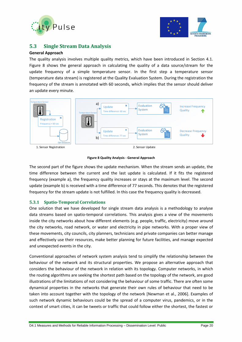
D4.1 Measures and Methods for Reliable Information Processing – Dissemination Level: Public Page 20
5.3 Single Stream Data Analysis General Approach
The quality analysis involves multiple quality metrics, which have been introduced in Section 4.1.
Figure 8 shows the general approach in calculating the quality of a data source/stream for the
update frequency of a simple temperature sensor. In the first step a temperature sensor
(temperature data stream) is registered at the Quality Evaluation System. During the registration the
frequency of the stream is annotated with 60 seconds, which implies that the sensor should deliver
an update every minute.
Figure 8 Quality Analysis - General Approach
The second part of the figure shows the update mechanism. When the stream sends an update, the
time difference between the current and the last update is calculated. If it fits the registered
frequency (example a), the frequency quality increases or stays at the maximum level. The second
update (example b) is received with a time difference of 77 seconds. This denotes that the registered
frequency for the stream update is not fulfilled. In this case the frequency quality is decreased.
5.3.1 Spatio-Temporal Correlations
One solution that we have developed for single stream data analysis is a methodology to analyse
data streams based on spatio-temporal correlations. This analysis gives a view of the movements
inside the city networks about how different elements (e.g. people, traffic, electricity) move around
the city networks, road network, or water and electricity in pipe networks. With a proper view of
these movements, city councils, city planners, technicians and private companies can better manage
and effectively use their resources, make better planning for future facilities, and manage expected
and unexpected events in the city.
Conventional approaches of network system analysis tend to simplify the relationship between the
behaviour of the network and its structural properties. We propose an alternative approach that
considers the behaviour of the network in relation with its topology. Computer networks, in which
the routing algorithms are seeking the shortest path based on the topology of the network, are good
illustrations of the limitations of not considering the behaviour of some traffic. There are often some
dynamical properties in the networks that generate their own rules of behaviour that need to be
taken into account together with the topology of the network [Newman et al., 2006]. Examples of
such network dynamic behaviours could be the spread of a computer virus, pandemics, or in the
context of smart cities, it can be tweets or traffic that could follow either the shortest, the fastest or
QoI Datastore
Temperature Sensor
Frequency = 60 sec
Registration
1. Sensor Registration
Temperature Sensor
2. Sensor Update
Time difference: 60 sec
Update EvaluationSystem
EvaluationSystem
Time difference: 77 sec
Update Decrease Frequency Quality
Increase Frequency Quality
a)
b)

D4.1 Measures and Methods for Reliable Information Processing – Dissemination Level: Public Page 21
the cheapest ways, which are not always coincident and might evolve depending on different
external circumstances. In these examples, following the spatial correlation will not be sufficient to
model the behaviour of the movements in a city. We show a more generalised behaviour of
movements adding a temporal component to the spatial correlation. This approach can be used to
model different environments. We apply it to create a spatio-temporal traffic model in smart cities.
Several studies have analysed city movements mostly with the idea of better structuring the cities
for future urban deployment [Bristow & Kennedy, 2013], [Weisz & Steinberger, 2010], [Yang &
Wong, 2013]). These studies have used different datasets and variables. For example, Roth et al. in
[Roth et al., 2011] study, where the people access and leave the London tube, and investigate the
different flows. Another work redraws the UK map based on human interactions by telephone calls
[Ratti et al., 2010]. These studies do not include the temporal or dynamic component of the
interactions or movements of interactions. The lack of attention to potential spread of changes in
the systems (e.g. unexpected events such as accidents, human reactions, or terrorist attacks at one
location may affect other locations of the network) limits the possibility of using the data for
accurate measures of security or rapid technical reaction, such as evacuation or replacement of
faulty services.
In vehicular traffic domain several works have studied the movement of traffic mainly based on
predicting the traffic at one particular point [Zheng et al., 2014]. Zheng et al. present a survey of the
latest applications in this field in urban environments. For example in [Mcardle et al., 2012] Mcardle
et al. study the wanders of people based on digital footprints, (e.g. twitter, foursquare) and simulate
the traffic based on the location of their houses and offices in the city. In these predictions usually
the traffic in previous moments of time and the neighbouring state of traffic is used [Chen & Zhang,
2014], [Asif et al., 2014], [Tchrakian et al., 2012]. However a full description of the movement of
traffic in a city has not been addressed to the best of the authors’ knowledge.
This description includes the impact that an event at one point of the city at a specific time will have
in the near future in another point of the city. Full description of flows will allow a better
management of unexpected events in the city, locating the emergency resources at the right
locations and at the right time. For that purpose it is worthy to study spatio-temporal correlations
that could give a clear relationship between two points of the city at different periods of time, and
how one can influence the other, giving a hint on the causation of a pattern in a specific point of the
city. Although we are not studying the causality, a well-known approach to get closer to causation is
to have sound methods and theories (e.g. [Williamson, 2011]), and by creating a model we are
getting closer to causality.
Compared to more complicated machine learning algorithms that require training adaptations and
are often limited in apply with the dynamicity of the data, we propose an efficient method to derive
spatio-temporal movements of the city using correlations, which are computationally effective. The
methodology, which is used to calculate data stream movement in the cities, is described in Figure 9.

D4.1 Measures and Methods for Reliable Information Processing – Dissemination Level: Public Page 22
Figure 9 Block Diagram of the Methodology to Calculate Data Stream Movements
Assuming we have sufficient data to divide it into windows and each window includes sufficient data
to measure correlations, we propose to use overlapping windows in order to improve the
measurements. In our example, we need to check if we have sufficient traffic in one week. We have
a dataset from the traffic in the city of Aarhus, in Denmark with 2.016 observations per week, and
we prove that this number is enough, because the correlation does not change substantially with a
week of sensory observations or with several months of sensory observations. Then, if we have
traffic for several weeks, we propose to improve the robustness of the correlation by making several
measurements and calculating the average of the result. In the following experiment we split the
streams into one-week windows. The block window splitter is configured with a window of
Δw =1 day. Then, we correlate the number of cars in two street sectors of the city for each day of
data (block correlation in Figure 9) with any correlation algorithm such as Pearson correlation or
mutual information. Then, we calculate the average correlation of all the measurement as the final
correlation of both sectors (block average correlation in Figure 9). With overlapping windows we can
reuse the observations for several experiments, virtually increasing the number of observations used
in the correlations. Figure 10 shows the plot of 4 weeks data of the number of car in one section of
one street in a city. We have divided this traffic in 50% overlap windows of one week each. As we
can see, Window2 is 50% overlap with Window1 and 50% overlap with Window3.
Figure 10 Four Weeks of Traffic Data Divided in Overlap Windows of 50%
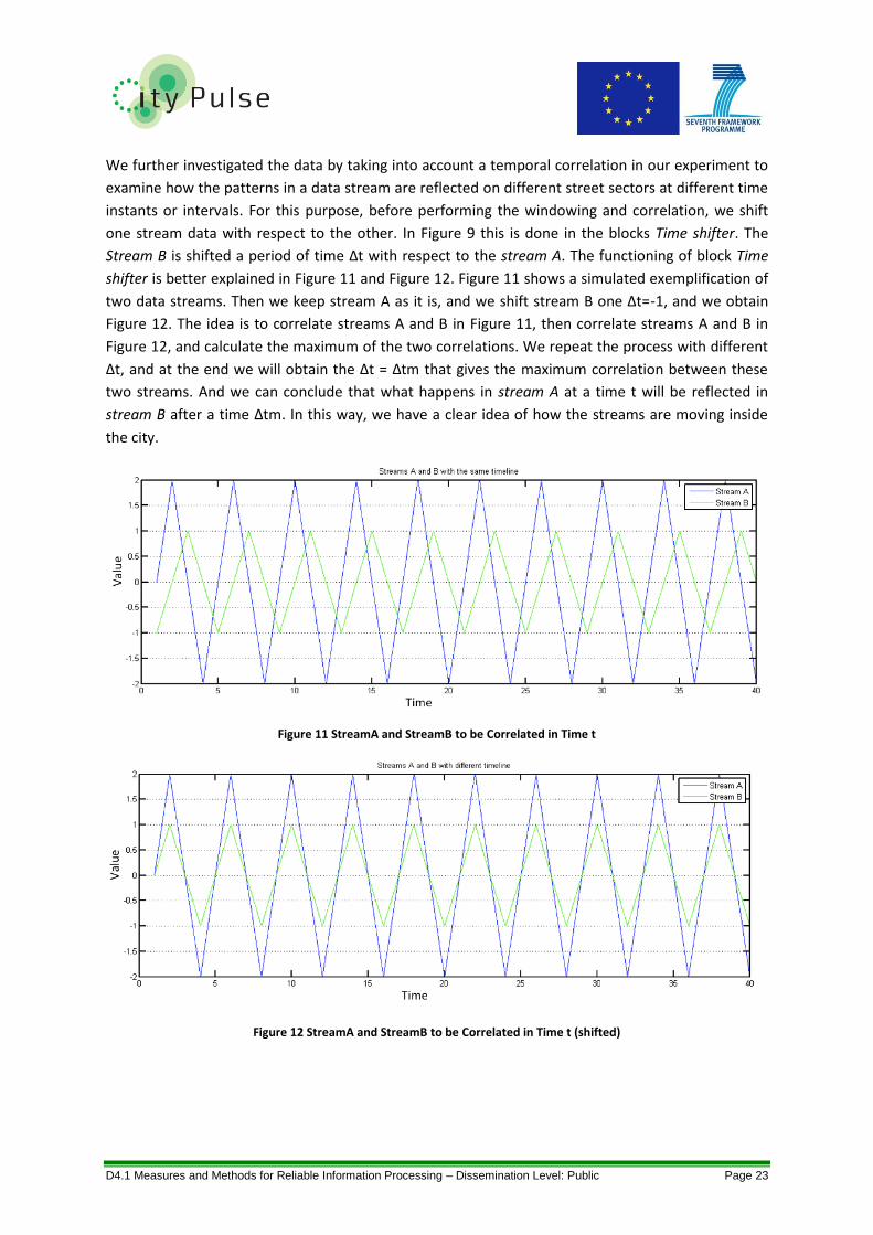
D4.1 Measures and Methods for Reliable Information Processing – Dissemination Level: Public Page 23
We further investigated the data by taking into account a temporal correlation in our experiment to
examine how the patterns in a data stream are reflected on different street sectors at different time
instants or intervals. For this purpose, before performing the windowing and correlation, we shift
one stream data with respect to the other. In Figure 9 this is done in the blocks Time shifter. The
Stream B is shifted a period of time Δt with respect to the stream A. The functioning of block Time
shifter is better explained in Figure 11 and Figure 12. Figure 11 shows a simulated exemplification of
two data streams. Then we keep stream A as it is, and we shift stream B one Δt=-1, and we obtain
Figure 12. The idea is to correlate streams A and B in Figure 11, then correlate streams A and B in
Figure 12, and calculate the maximum of the two correlations. We repeat the process with different
Δt, and at the end we will obtain the Δt = Δtm that gives the maximum correlation between these
two streams. And we can conclude that what happens in stream A at a time t will be reflected in
stream B after a time Δtm. In this way, we have a clear idea of how the streams are moving inside
the city.
Figure 11 StreamA and StreamB to be Correlated in Time t
Figure 12 StreamA and StreamB to be Correlated in Time t (shifted)
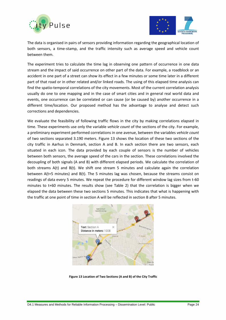
D4.1 Measures and Methods for Reliable Information Processing – Dissemination Level: Public Page 24
The data is organised in pairs of sensors providing information regarding the geographical location of
both sensors, a time-stamp, and the traffic intensity such as average speed and vehicle count
between them.
The experiment tries to calculate the time lag in observing one pattern of occurrence in one data
stream and the impact of said occurrence on other part of the data. For example, a roadblock or an
accident in one part of a street can show its effect in a few minutes or some time later in a different
part of that road or in other related and/or linked roads. The using of this elapsed time analysis can
find the spatio-temporal correlations of the city movements. Most of the current correlation analysis
usually do one to one mapping and in the case of smart cities and in general real world data and
events, one occurrence can be correlated or can cause (or be caused by) another occurrence in a
different time/location. Our proposed method has the advantage to analyse and detect such
corrections and dependencies.
We evaluate the feasibility of following traffic flows in the city by making correlations elapsed in
time. These experiments use only the variable vehicle count of the sections of the city. For example,
a preliminary experiment performed correlations in one avenue, between the variables vehicle count
of two sections separated 3.190 meters. Figure 13 shows the location of these two sections of the
city traffic in Aarhus in Denmark, section A and B. In each section there are two sensors, each
situated in each icon. The data provided by each couple of sensors is the number of vehicles
between both sensors, the average speed of the cars in the section. These correlations involved the
decoupling of both signals (A and B) with different elapsed periods. We calculate the correlation of
both streams A(t) and B(t). We shift one stream 5 minutes and calculate again the correlation
between A(t+5 minutes) and B(t). The 5 minutes lag was chosen, because the streams consist on
readings of data every 5 minutes. We repeat the procedure for different window lag sizes from t-60
minutes to t+60 minutes. The results show (see Table 2) that the correlation is bigger when we
elapsed the data between these two sections 5 minutes. This indicates that what is happening with
the traffic at one point of time in section A will be reflected in section B after 5 minutes.
Figure 13 Location of Two Sections (A and B) of the City Traffic
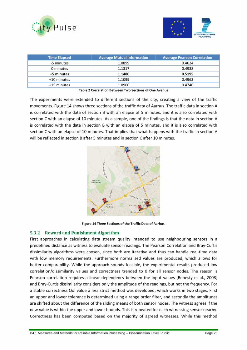
D4.1 Measures and Methods for Reliable Information Processing – Dissemination Level: Public Page 25
Time Elapsed Average Mutual Information Average Pearson Correlation
-5 minutes 1.0899 0.4624
0 minutes 1.1317 0.4938
+5 minutes 1.1480 0.5195
+10 minutes 1.1099 0.4963
+15 minutes 1.0900 0.4740 Table 2 Correlation Between Two Sections of One Avenue
The experiments were extended to different sections of the city, creating a view of the traffic
movements. Figure 14 shows three sections of the traffic data of Aarhus. The traffic data in section A
is correlated with the data of section B with an elapse of 5 minutes, and it is also correlated with
section C with an elapse of 10 minutes. As a sample, one of the findings is that the data in section A
is correlated with the data in section B with an elapse of 5 minutes, and it is also correlated with
section C with an elapse of 10 minutes. That implies that what happens with the traffic in section A
will be reflected in section B after 5 minutes and in section C after 10 minutes.
Figure 14 Three Sections of the Traffic Data of Aarhus.
5.3.2 Reward and Punishment Algorithm
First approaches in calculating data stream quality intended to use neighbouring sensors in a
predefined distance as witness to evaluate sensor readings. The Pearson Correlation and Bray-Curtis
dissimilarity algorithms were chosen, since both are iterative and thus can handle real-time data
with low memory requirements. Furthermore normalised values are produced, which allows for
better comparability. While the approach sounds feasible, the experimental results produced low
correlation/dissimilarity values and correctness trended to 0 for all sensor nodes. The reason is
Pearson correlation requires a linear dependency between the input values [Benesty et al., 2008]
and Bray-Curtis dissimilarity considers only the amplitude of the readings, but not the frequency. For
a stable correctness QoI value a less strict method was developed, which works in two stages. First
an upper and lower tolerance is determined using a range order filter, and secondly the amplitudes
are shifted about the difference of the sliding means of both sensor nodes. The witness agrees if the
new value is within the upper and lower bounds. This is repeated for each witnessing sensor nearby.
Correctness has been computed based on the majority of agreed witnesses. While this method

D4.1 Measures and Methods for Reliable Information Processing – Dissemination Level: Public Page 26
provides stable QoI values, it also provides configuration abilities (e.g. window size of the range
order filter, offset for upper and lower bound) to adapt easily to different scenarios (compare
Section 5.3.2.1, Figure 18). The goal of the quality analysis is to produce a metric, which indicates the
current performance of a sensor node compared with promised quality metrics annotated during
the registration process. This metric can either be the absolute value of a specific QoI metric or a
normalised value. An advantage of using a normalised value is a) that sensor nodes of different
providers can be compared and b) different QoI metrics can be combined to derive an overall
reputation metric for a sensor node or network. To calculate the normalised value, an algorithm
with the following properties was designed. The output of the algorithm is in the range of 0 and 1.
The input is a discrete value and indicates if the last observation update satisfies the annotated
quality metric. The output is increased if the input was positive and vice versa, with respect to the
output value range. The algorithm considers past behaviour of the sensor node, so that continuous
reliability results in a higher output. The magnitude of a negative input decreases over time. At the
same time it allows to fully recover from negative inputs, such as sporadic outliers, after a series of
observation updates. The algorithm requires a constant amount of memory and processing power.
The implementation is a modified version of a reward and punishment algorithm introduced by
[Hossain et al, 2011]. It uses a sliding window over the last inputs with window length W. The quality
metric is calculated as follows:
Equation 1
where q(t) is the quality metric at time t and q(t − 1) is the past quality metric. Rd(t) denotes the reward to be added for the current input. The reward is calculated as:
Equation 2
denotes the number of positive entries within the window and the current
input.
5.3.2.1 Reward and Punishment Evaluation on Reference Data
In the Reward and Punishment Evaluation experiments, a subset of QoI metrics is used, which are
introduced in Table 1. The QoI metrics in the context of the ODAA Aarhus traffic data are calculated
as follows:
Completeness
Each observation within the data feed is composed of a set of features. An observation is considered
complete if all features are present and contains valid values, so that the Reward & Punishment
algorithm is positive, otherwise negative. The validity of a feature has to be defined depending on
the context. As an example it has to be decided, if an empty string is interpreted as a valid attribute
or the absence of it. The Aarhus traffic sensor network in our experiment used a web service as
bridge to provide access to the sensor network. Direct access to the sensor nodes was not possible.
Since the web service always delivered the last observations, completeness in our experiment was
always 100%. Omitted observations only affected the Frequency metric.

D4.1 Measures and Methods for Reliable Information Processing – Dissemination Level: Public Page 27
Frequency
To evaluate the frequency of an observation two basic approaches can be used. In case the sensor
node pushes update notifications the difference between two successive notifications results in the
frequency. In case of a pull mechanism a request after the maximum frequency, as annotated during
registration, should always return an updated observation. Here, the initial annotated frequency
indicates the update interval. In case a time stamp is present the determination of the frequency can
be simplified as the difference of the time stamps of two successive observations. For the Aarhus
experiment, a gateway web service delivered the last observation if no update from the sensor node
was received. Here a further constraint has to be made. That is the time difference must be higher
than 0 and lower or equal than the initial annotated frequency. In the experiment 449 sensor nodes
were observed, each reporting every 5 minutes over a period of 31 days resulting in a bit over 4
million frequency QoI annotations. Figure 15 shows the distribution of QoI values annotated during
the experiment. As shown about 75% have been rated with 0.95 or higher and almost 95% have
been rated 0.8 or higher.
Figure 15 Histogram Distribution of Frequency QoI Value Classes
Figure 16 depicts the average frequency QoI value per sensor and how many sensors reach the
average. About 50 of the 449 sensor nodes have an average frequency QoI value of 0.9 or less, but
still over 0.85. About 290 sensor nodes, more than half of the sensor nodes observed during the
experiment, could reach an average frequency QoI of 0.95 or higher.
0
1000000
2000000
3000000
0.00 0.25 0.50 0.75 1.00
Frequency QoI Value
Num
ber
of O
ccure
nce

D4.1 Measures and Methods for Reliable Information Processing – Dissemination Level: Public Page 28
Figure 16 Average Frequency per Sensor
Correctness
It is a well-known fact in the meteorology community that it is impossible to measure real world
physical values free of errors. Many error sources (e.g. noise, drift, ageing of the sensing equipment)
influence the measurements in a random and unpredictable way. Depending on the available
information, different strategies to compensate for those influences can be applied. Investigating a
single sensor reading allows only validation against possible and probable value ranges. Considering
a series of observations of a single sensor allows to check if the sensor got stuck at a certain value or
to detect outliers (such as sudden spikes). If multiple sensors are available a common strategy is to
use redundant sensors, measuring the same or a correlated value and to perform validations
between both sensors. In our experiment the 3 nearest neighbouring sensors are used to evaluate
the correctness of each observation.
An exemplarily evaluation of 2 nearby sensors (see Figure 17), which is utilised by the Reward and
Punishment algorithm, is shown in Figure 18. The value changes of sensor 158565 are continuously
checked against sensor 158446, which is connected on a joining road section. The Figure shows the
original measurements of both sensors (blue and green lines) and the upper and lower boundaries
(red and black lines) with shifted amplitudes. Although the amplitudes are significantly different,
70.6% of the sensor 158565 measurements are within the calculated boundaries.
Figure 17 Sensor Node Measuring Direction
0.80
0.85
0.90
0.95
1.00
0 100 200 300 400
# of nodes with at least this average
Ave
rag
e F
req
uen
cy Q
oI
Valu
e
Sensor 158565Sensor 158446
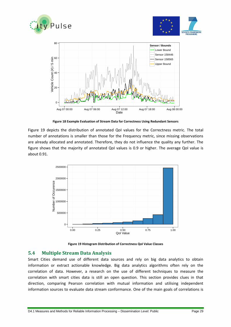
D4.1 Measures and Methods for Reliable Information Processing – Dissemination Level: Public Page 29
Figure 18 Example Evaluation of Stream Data for Correctness Using Redundant Sensors
Figure 19 depicts the distribution of annotated QoI values for the Correctness metric. The total
number of annotations is smaller than those for the Frequency metric, since missing observations
are already allocated and annotated. Therefore, they do not influence the quality any further. The
figure shows that the majority of annotated QoI values is 0.9 or higher. The average QoI value is
about 0.91.
Figure 19 Histogram Distribution of Correctness QoI Value Classes
5.4 Multiple Stream Data Analysis Smart Cities demand use of different data sources and rely on big data analytics to obtain
information or extract actionable knowledge. Big data analytics algorithms often rely on the
correlation of data. However, a research on the use of different techniques to measure the
correlation with smart cities data is still an open question. This section provides clues in that
direction, comparing Pearson correlation with mutual information and utilising independent
information sources to evaluate data stream conformance. One of the main goals of correlations is
0
20
40
60
80
Aug 07 00:00 Aug 07 06:00 Aug 07 12:00 Aug 07 18:00 Aug 08 00:00
Date
Ve
hic
le C
ou
nt
(#)
/ 5
min
Sensor / Bounds
Lower Bound
Sensor 158446
Sensor 158565
Upper Bound
0
500000
1000000
1500000
2000000
2500000
0.00 0.25 0.50 0.75 1.00
QoI Value
Num
ber
of O
ccure
nce
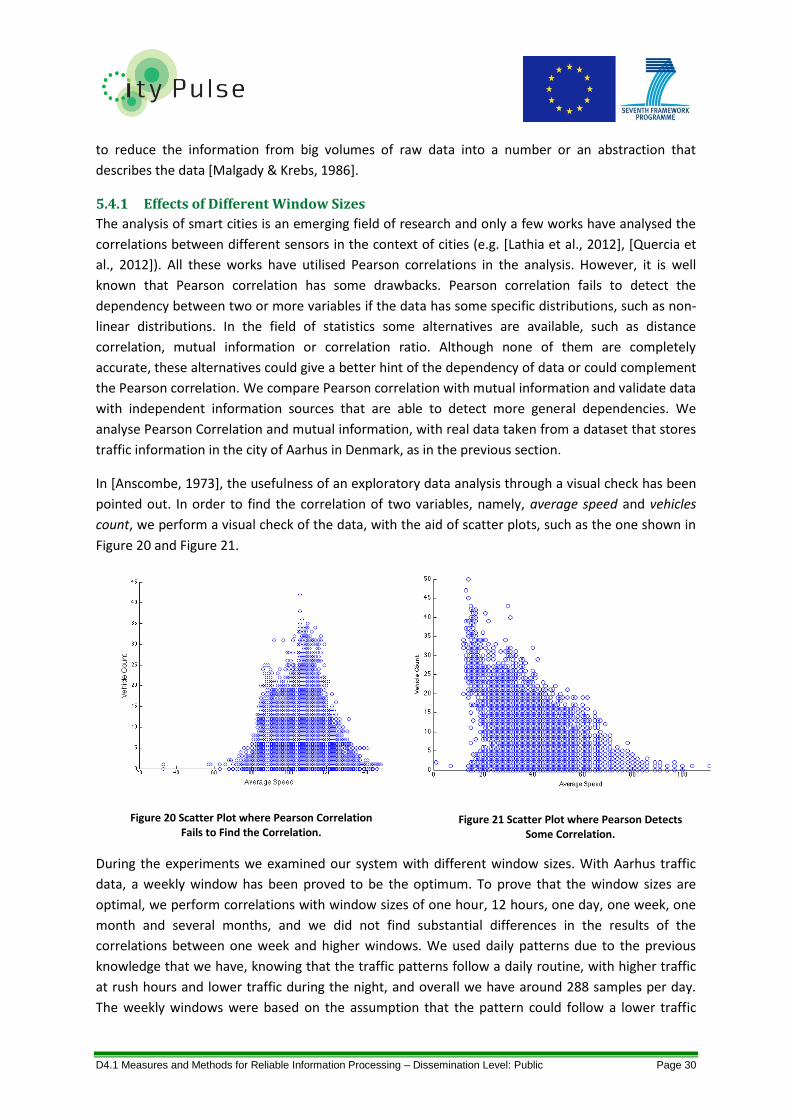
D4.1 Measures and Methods for Reliable Information Processing – Dissemination Level: Public Page 30
to reduce the information from big volumes of raw data into a number or an abstraction that
describes the data [Malgady & Krebs, 1986].
5.4.1 Effects of Different Window Sizes
The analysis of smart cities is an emerging field of research and only a few works have analysed the
correlations between different sensors in the context of cities (e.g. [Lathia et al., 2012], [Quercia et
al., 2012]). All these works have utilised Pearson correlations in the analysis. However, it is well
known that Pearson correlation has some drawbacks. Pearson correlation fails to detect the
dependency between two or more variables if the data has some specific distributions, such as non-
linear distributions. In the field of statistics some alternatives are available, such as distance
correlation, mutual information or correlation ratio. Although none of them are completely
accurate, these alternatives could give a better hint of the dependency of data or could complement
the Pearson correlation. We compare Pearson correlation with mutual information and validate data
with independent information sources that are able to detect more general dependencies. We
analyse Pearson Correlation and mutual information, with real data taken from a dataset that stores
traffic information in the city of Aarhus in Denmark, as in the previous section.
In [Anscombe, 1973], the usefulness of an exploratory data analysis through a visual check has been
pointed out. In order to find the correlation of two variables, namely, average speed and vehicles
count, we perform a visual check of the data, with the aid of scatter plots, such as the one shown in
Figure 20 and Figure 21.
Figure 20 Scatter Plot where Pearson Correlation Fails to Find the Correlation.
Figure 21 Scatter Plot where Pearson Detects Some Correlation.
During the experiments we examined our system with different window sizes. With Aarhus traffic
data, a weekly window has been proved to be the optimum. To prove that the window sizes are
optimal, we perform correlations with window sizes of one hour, 12 hours, one day, one week, one
month and several months, and we did not find substantial differences in the results of the
correlations between one week and higher windows. We used daily patterns due to the previous
knowledge that we have, knowing that the traffic patterns follow a daily routine, with higher traffic
at rush hours and lower traffic during the night, and overall we have around 288 samples per day.
The weekly windows were based on the assumption that the pattern could follow a lower traffic
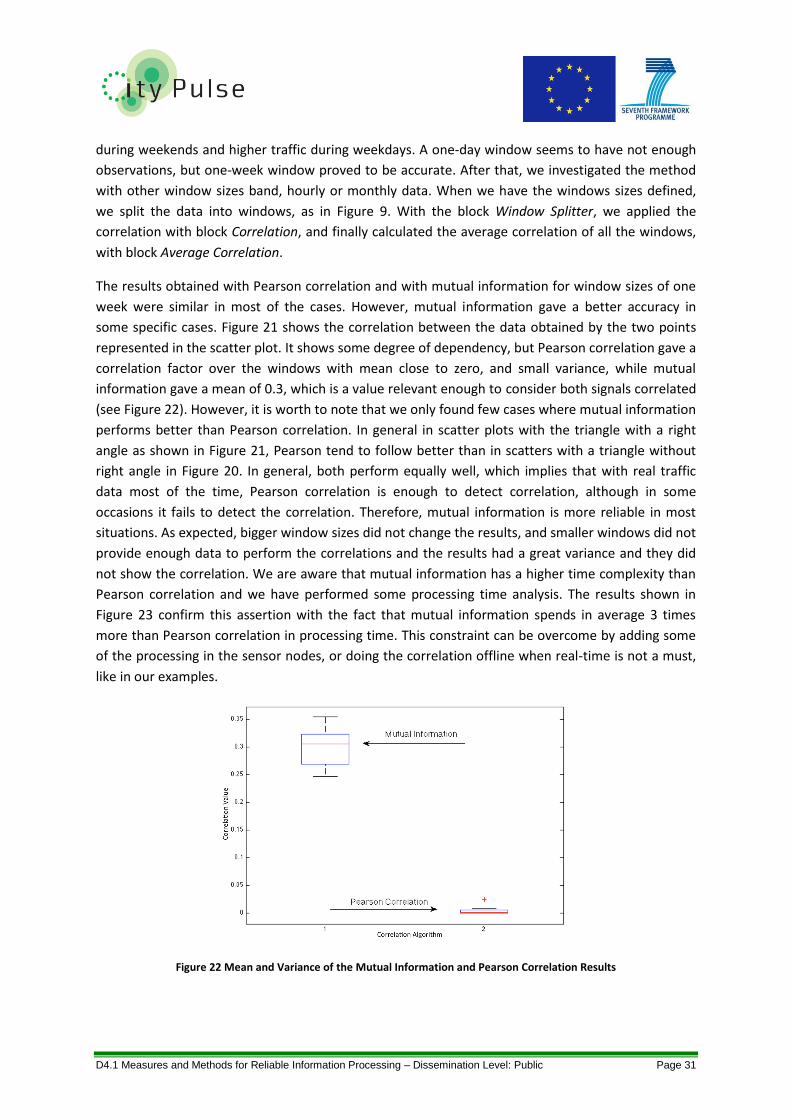
D4.1 Measures and Methods for Reliable Information Processing – Dissemination Level: Public Page 31
during weekends and higher traffic during weekdays. A one-day window seems to have not enough
observations, but one-week window proved to be accurate. After that, we investigated the method
with other window sizes band, hourly or monthly data. When we have the windows sizes defined,
we split the data into windows, as in Figure 9. With the block Window Splitter, we applied the
correlation with block Correlation, and finally calculated the average correlation of all the windows,
with block Average Correlation.
The results obtained with Pearson correlation and with mutual information for window sizes of one
week were similar in most of the cases. However, mutual information gave a better accuracy in
some specific cases. Figure 21 shows the correlation between the data obtained by the two points
represented in the scatter plot. It shows some degree of dependency, but Pearson correlation gave a
correlation factor over the windows with mean close to zero, and small variance, while mutual
information gave a mean of 0.3, which is a value relevant enough to consider both signals correlated
(see Figure 22). However, it is worth to note that we only found few cases where mutual information
performs better than Pearson correlation. In general in scatter plots with the triangle with a right
angle as shown in Figure 21, Pearson tend to follow better than in scatters with a triangle without
right angle in Figure 20. In general, both perform equally well, which implies that with real traffic
data most of the time, Pearson correlation is enough to detect correlation, although in some
occasions it fails to detect the correlation. Therefore, mutual information is more reliable in most
situations. As expected, bigger window sizes did not change the results, and smaller windows did not
provide enough data to perform the correlations and the results had a great variance and they did
not show the correlation. We are aware that mutual information has a higher time complexity than
Pearson correlation and we have performed some processing time analysis. The results shown in
Figure 23 confirm this assertion with the fact that mutual information spends in average 3 times
more than Pearson correlation in processing time. This constraint can be overcome by adding some
of the processing in the sensor nodes, or doing the correlation offline when real-time is not a must,
like in our examples.
Figure 22 Mean and Variance of the Mutual Information and Pearson Correlation Results
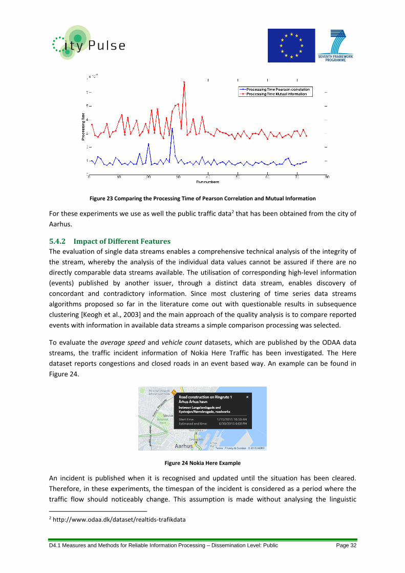
D4.1 Measures and Methods for Reliable Information Processing – Dissemination Level: Public Page 32
Figure 23 Comparing the Processing Time of Pearson Correlation and Mutual Information
For these experiments we use as well the public traffic data2 that has been obtained from the city of
Aarhus.
5.4.2 Impact of Different Features
The evaluation of single data streams enables a comprehensive technical analysis of the integrity of
the stream, whereby the analysis of the individual data values cannot be assured if there are no
directly comparable data streams available. The utilisation of corresponding high-level information
(events) published by another issuer, through a distinct data stream, enables discovery of
concordant and contradictory information. Since most clustering of time series data streams
algorithms proposed so far in the literature come out with questionable results in subsequence
clustering [Keogh et al., 2003] and the main approach of the quality analysis is to compare reported
events with information in available data streams a simple comparison processing was selected.
To evaluate the average speed and vehicle count datasets, which are published by the ODAA data
streams, the traffic incident information of Nokia Here Traffic has been investigated. The Here
dataset reports congestions and closed roads in an event based way. An example can be found in
Figure 24.
Figure 24 Nokia Here Example
An incident is published when it is recognised and updated until the situation has been cleared.
Therefore, in these experiments, the timespan of the incident is considered as a period where the
traffic flow should noticeably change. This assumption is made without analysing the linguistic
2 http://www.odaa.dk/dataset/realtids-trafikdata

D4.1 Measures and Methods for Reliable Information Processing – Dissemination Level: Public Page 33
incident description (e.g. “Traffic problem. Temporary bicycle parking.” and “Traffic problem. Buses
and occupant driving exempted. Events in Memorial Park.” (Translated from Danish: “Trafik
problem. Midlertidig cykelparkering.” and “Trafik problem. Busser og beboer korsel undtaget.
Arrangement i Mindeparken.”). To find events that could be evaluated with the ODAA traffic
sensors, the direction and distance in relationship to the traffic sensors are considered to find
comparable data segments.
The incident dataset describes the start time tIstart and the end time tIend of the congestion incident,
which defines the incident period pI=[tIstart,tIend] with the duration dI of the incident. To evaluate the
dependency between the streams, the seasonally adjusted time series of the average speed is
investigated for pBefore=[tIstart - dIncident, tIstart) before and for pAfter=(tIend, tIend + dIncident) after the
congestion period pIncident. The quartiles Q1, Q2 and Q3 (the 25th, 50th (median) and 75th
percentiles) of pI and pBefore. are now compared against each other. If the incident already ended and
there is subsequent traffic data available, pI is also compared to pAfter (see Figure 25).
Figure 25 Comparing Traffic Flow Before, During, and After a Traffic Incident
If the majority of quartiles (at least 2) leads to an increase of the average speed from pBefore to pI and
a decrease from pI to pAfter, a conformance in the expected behaviour is detected. This leads to a
consolidation of the correctness level of the stream and can also lead to an increase of the
reputation level of the information source.
The evaluation of the comparison of 25 distinct traffic incidents against the ODAA data shows only
76% conformity between traffic incident reports and ODAA traffic using the raw data. By taking into
account the results of the Frequency QoI analysis (see Section 5.3.2), missing data can be identified
as a cause of this low conformity. By ignoring ODAA streams that had noticeable faults within single
stream quality analysis, the conformance increases to 83%.
●
●
●
●
●●
●●
●●
●
●
●
●
●●
●●
●
●
●
●
●
●●●
0
20
40
60
Sep 01 Sep 03 Sep 05 Sep 07 Sep 09
Measurement Date
Ve
hic
le C
ou
nt
(cars
/15
min
)
●
●
●●●●
●●●
●
20
40
60
80
Sep 01 Sep 03 Sep 05 Sep 07 Sep 09
Measurement Date
Avera
ge V
eh
icle
Sp
ee
d (
km
/h)
Measurement Period: after incident before incident during incident
D4.1 Measures and Methods for Reliable Information Processing – Dissemination Level: Public Page 34
5.5 Dynamic Semantics for Smart City Data in Constrained Environments Smart City data is highly variable in terms of dynamicity, granularity, and quality. The available data,
in general terms, does not cover the whole city area with the same quality. The QoI is therefore
spatio-temporal dependant. Some smart city frameworks, rely on semantic descriptions of data,
which are static by nature and it is difficult to accommodate in them the spatio-temporal changes of
the QoI. We propose dynamic semantics based on mathematical expressions through MathML to
specify the interpolation of the available data for better representation of the spatial and temporal
changes of the data. Likewise, dynamic semantics allow the dynamic description of the QoI in terms
of location and time.
QoI is variable on time and location. Depending on the timeliness of the data the quality varies; for
example, the quality of the temperature value is not the same if it was taken 2 minutes ago or if the
value was taken one hour ago. Likewise QoI also depends on the location (e.g. the value of a
temperature sensor that covers an area of the city will be more accurate 1 metre away from the
sensor than half a kilometre away). Due to these variety of data and QoI, it is difficult to have
accurate values that cover the entire city in real-time. Therefore for some applications it should be
worthy to interpolate the available values in time and location to cover the whole city at any time.
Prominent smart city frameworks rely on semantics (e.g. SmartSantander [Turchi et al., 2014]),
which provide an annotation model to support interoperability and knowledge based information
fusion between different sources of information. However the semantic descriptions that are
provided for the smart city data do not embody formulas for dynamic environments in which the
properties and QoI related attributes of data might change over time and in different locations.
Most of the current semantic annotation techniques and semantic description frameworks are static
and are based on the assumption that the information will not change over time. Although, some
researchers have faced the problems of dealing with dynamic data stored in semantic descriptions,
none of them, to the best of our knowledge, has thought of providing the dynamicity inside the
triple-store. Most of the solutions available for semantic descriptions deal with dynamic data that is
based on REST (Representational State Transfer) [Pautasso, 2014]. These solutions store a Unified
Resource Identifier (URI), with the RESTful interface in the triple-store which links to a web service
(e.g. [Janowicz et al., 2013], [Muller et al., 2013]). The web service can provide direct access to the
dynamic data, or to some abstraction of the dynamic data. However, these solutions are not suitable
for low connectivity networks or high frequency queries. In RESTful web services, when a user sends
a query, the query has to access the triple-store and also the server, which provides the web service.
All this time spent in the communication could be essential in applications with real-time constrains
or in networks with intermittent or low bandwidth connectivity. Other attempts to handle dynamic
data in semantics are based on reasoning. For example, Baader et al., have introduced the
temporised description logic, which provides semantic reasoning with some temporal component
[Baader et al., 2012]. Most of the current reasoning engines are not efficient in dealing with high
volumes of queries with real-time requirements. Therefore, the problem of accessing the current
dynamic data in extreme conditions (real-time constraints and low connectivity) remains unsolved.

D4.1 Measures and Methods for Reliable Information Processing – Dissemination Level: Public Page 35
Another line of research has implemented formulas, as rules, inside the semantic descriptions [Lopez
et al., 1999]. However these formulas are static, they do not have spatio-temporal components, and
its execution is done with a low frequency. The execution of the formulas in this solution needs to be
done by reasoner engines, because they are represented as rules. Therefore, as stated in the
paragraph above, this solution is not optimal for smart city scenarios, with high volume of users and
data. Our proposal differs from the previous works in a way that is a dynamic description, where the
dynamicity is stored inside the triple-store as a MathML formula. This formula can be executed
outside the semantic description, avoiding the long processing time of the semantic reasoners, but
at the same time avoiding the need to access the data or the abstraction of the data in another
server (such as RESTful solutions). Furthermore, our approach stores all the information about an IoT
entity at the same place, instead of storing different attributes of the IoT entity, such as sensed
value, reliability of the value, timeliness of the value or provenance on different servers (as RESTful
solutions do).
For that reason, we believe that the semantic descriptions should include the interpolation
functions, avoiding the connection to other servers to access more information and to reconstruct
the missing data, and therefore shorten the response time of the queries, especially for networks
with intermittent connections or low bandwidth. We propose using dynamic semantics, which
describe dynamic functions to interpolate, reconstruct or validate the available data in order to have
a bigger spatio-temporal coverage, in environments with missing values or low spatial and/or
temporal granularity. The proposal borrows some principles of the transition between the static and
dynamic web where elements such as MathML3 are key elements.
As HTML5 has enhanced and embedded the local availability of dynamicity and context awareness,
we envision the future semantic triple-stores to be dynamic. Our proposal is the first step in that
direction including formulas in triple-stores that can represent the dynamicity of the data stored in
the triple-store. These formulas provide the tools for context aware applications. In our proposal the
formulas in the triple-store are represented in MathML, which is the most spread common
representation of mathematical formulas, and already has existing translation libraries for the main
languages, Java, Python, C++, etc., into MathML and vice-versa. The representation of the formulas
inside the triple-stores has some advantages over other solutions that keep the triple-store static
(such as solutions using an URL pointing to a RESTful web service where the formulas can be
executed). In the case of dynamic semantics, the response time for a query will be lower as all the
processing is done locally. Alternative solutions, such as RESTful web services, will require more time
for the query to be answered, due to the need to access different servers that handle the web
services. Dynamic semantics does not need to access other web services on other servers, and stores
locally all the information related to the sensed entity. Our approach follows the philosophy of
linked data [Bizer et al., 2009], although the linked data could be locally stored on one server. We
propose to create a module to store formulas that could be reused for other sensor entities stored in
the same or different triple-store. This module is used together with main modules of CityPulse
[Kolozali et al., 2014]. The annotation of the data module describes the stream of a sensor and the
last value annotated together with its timestamp and a link to the formula module.
3 http://www.w3.org/TR/MathML3/ MathML is a common language to describe mathematical expressions.
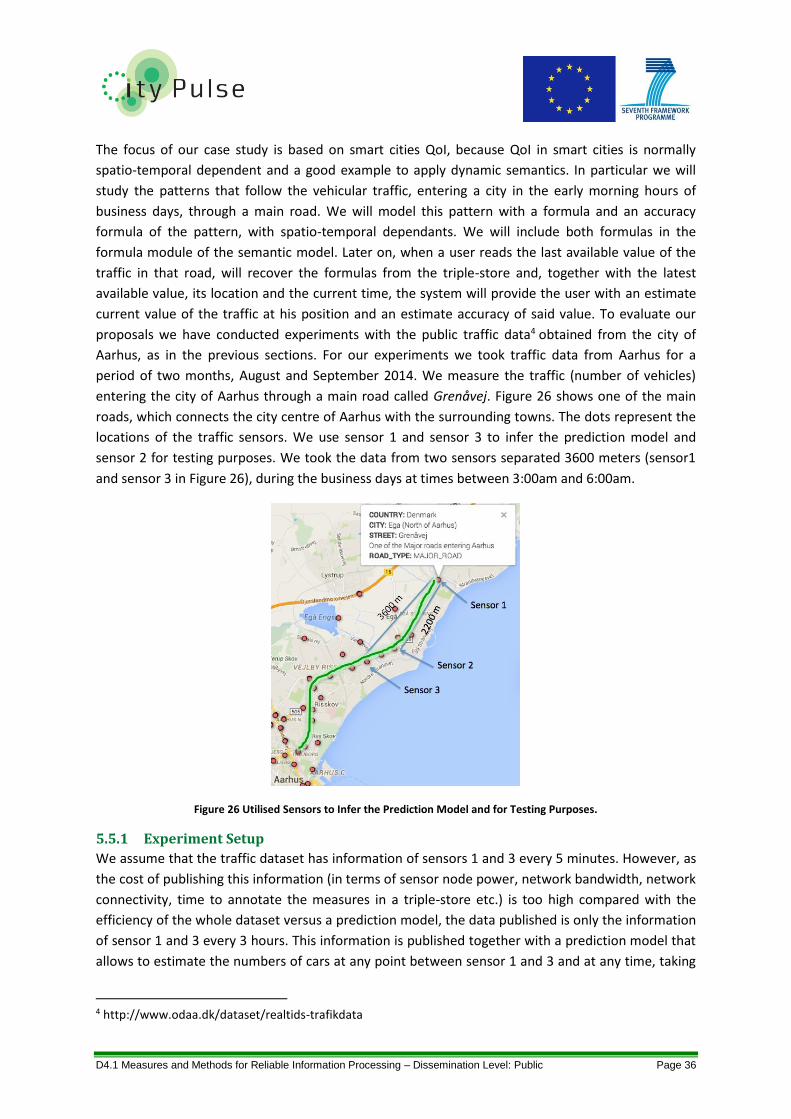
D4.1 Measures and Methods for Reliable Information Processing – Dissemination Level: Public Page 36
The focus of our case study is based on smart cities QoI, because QoI in smart cities is normally
spatio-temporal dependent and a good example to apply dynamic semantics. In particular we will
study the patterns that follow the vehicular traffic, entering a city in the early morning hours of
business days, through a main road. We will model this pattern with a formula and an accuracy
formula of the pattern, with spatio-temporal dependants. We will include both formulas in the
formula module of the semantic model. Later on, when a user reads the last available value of the
traffic in that road, will recover the formulas from the triple-store and, together with the latest
available value, its location and the current time, the system will provide the user with an estimate
current value of the traffic at his position and an estimate accuracy of said value. To evaluate our
proposals we have conducted experiments with the public traffic data4 obtained from the city of
Aarhus, as in the previous sections. For our experiments we took traffic data from Aarhus for a
period of two months, August and September 2014. We measure the traffic (number of vehicles)
entering the city of Aarhus through a main road called Grenåvej. Figure 26 shows one of the main
roads, which connects the city centre of Aarhus with the surrounding towns. The dots represent the
locations of the traffic sensors. We use sensor 1 and sensor 3 to infer the prediction model and
sensor 2 for testing purposes. We took the data from two sensors separated 3600 meters (sensor1
and sensor 3 in Figure 26), during the business days at times between 3:00am and 6:00am.
Figure 26 Utilised Sensors to Infer the Prediction Model and for Testing Purposes.
5.5.1 Experiment Setup
We assume that the traffic dataset has information of sensors 1 and 3 every 5 minutes. However, as
the cost of publishing this information (in terms of sensor node power, network bandwidth, network
connectivity, time to annotate the measures in a triple-store etc.) is too high compared with the
efficiency of the whole dataset versus a prediction model, the data published is only the information
of sensor 1 and 3 every 3 hours. This information is published together with a prediction model that
allows to estimate the numbers of cars at any point between sensor 1 and 3 and at any time, taking
4 http://www.odaa.dk/dataset/realtids-trafikdata

D4.1 Measures and Methods for Reliable Information Processing – Dissemination Level: Public Page 37
into account the last measurement stored in the triple-store. The data can be used to infer different
models for different periods of times (0:00am-3:00am; 3:00am-6:00am, etc.), making the distinction
between business days and holidays, due to the different patterns in traffic. A unique vehicular
prediction model could be feasible, but for clarity reasons and in order to keep focus on the dynamic
semantics, and not in traffic modelling, we will assume different simple models. Now, we show the
process to create and annotate the prediction model with its predicted accuracy model, valid for the
time period between 3:00am and 6:00am on business days. We annotate the last values (values at
3:00am) in the CityPulse information models, and link the prediction model to a formula module. We
linked also the prediction model (also in the formula module) with the QoI module of CityPulse
[Iggena et al., 2014]. We will use the concept accuracy of the QoI module to make the link with the
accuracy modelled. To this end, the first step is to create the prediction models. We will use linear
interpolation models, which can be used as a basic prediction model. Later on, we evaluate the
model assuming that we want to know the number of cars during one business day at the same
position of sensor 2 (see Figure 26) with the prediction model, assuming that the last annotated
value of sensor 1 is at 3:00am. We compare the predictions obtained with the prediction models
every 5 minutes from 3:00am to 6:00am with the real values obtained by reading sensor 2.
5.5.2 Experiments
The first step in our experiment is to create the prediction model that will be composed of two linear
interpolation models, one for the spatial component and the other for the temporal component of
the prediction model. We calculate the temporal component of the prediction model and the
prediction accuracy. For that purpose we take data only from sensor 1 (see Figure 26) at 3:00am and
at 6:00am on business days. Before processing the data we need a pre-processing. We have
observed some problems with the data that can be overcome with the pre-processing. In some cases
our dataset has missing values. For example the data missed a few values in a day. If the data does
not have any value at 3:00am or at 6:00am with our approach of linear interpolation, we missed the
whole day. Another problem is the irregularity of the number of vehicles. Although the traffic follow
is a pattern, and the trend is a positive increment in the number of vehicles when the time changes
from 3:00am to 6:00am, this tendency is not strictly observed every 5 minutes. That means that
although in general terms the traffic trend increases, it is quite frequent to have a decrease between
two subsequent measurements. In order to smooth the data and take more accurate values, instead
of taken just the value at 3:00, we have taken values of the cars at 2:55, 3:00 and 3:05 and perform
the average of this values before processing the data. The same process is also repeated for the
values in the time range of 5:55 and 6:05. This pre-processing does not bias the results, because our
final aim is not to have an exact value, but to infer the tendency of the data. After the pre-
processing, for each day we calculate the difference between the number of cars at 6:00am and at
3:00am. Then, we calculate the average and the standard deviation of this difference taking into
account all the days. The average of this difference is represented as V6-V3 in Figure 27. After that we
perform a linear interpolation model between the average of the vehicles at 3:00am Vc and the
average of the difference in number of vehicles between 6:00am and 3:00am V6-V3. We apply linear
interpolation (Equation 3), but this time the values will be t3 representing time at 3:00am, V3
representing average in number of vehicles in sensor 1 at 3:00am, t6 representing time at 6:00am, V6

D4.1 Measures and Methods for Reliable Information Processing – Dissemination Level: Public Page 38
representing average of the number of vehicles in sensor 1 at 6:00am, tx a time x between 3:00am
and 6:00am, and Vx the number of cars at a time x.
Figure 27 Linear Interpolation for the Temporal Component of the Prediction Model
Equation 3
Similarly we calculate the spatial component. For that purpose we calculate the average of the
number of cars in sensor 1, V1, and the mean of the difference between sensor 3 and sensor 1,
taking into account every 5 minutes the pair of points V1 V3. The resulting spatial component is
depicted in Equation 4 where Sx represents location x between location of sensor 1, S1 and location
of sensor 3, S3.
Now, adding both components we have:
Equation 4
In a similar manner we calculate the spatial and temporal components of the accuracy of the values.
In this case instead of taken the means of the values we take the standard deviation (STD) of the
values, and we end up with a similar formula.
Now, we take the time in minutes and the distance in meters. The distance between sensor 1 and
sensor 3 is 3600 meters, and the difference in minutes between 3:00am and 6:00am is 180 minutes.
The time in minutes at 3:00am (minutes between 00:00 and 03:00) is 180 minutes, and at 6:00am is
360 minutes. The mean and the STD that we have calculated are: average (V6-V3) = 24.7764227642,
average(VS3-VS1)= 2.75518672199, STD(V6-V3)= 4.83867237442, STD(VS3-VS1)= 6.04280123937. With
this values the resulting formulas are:
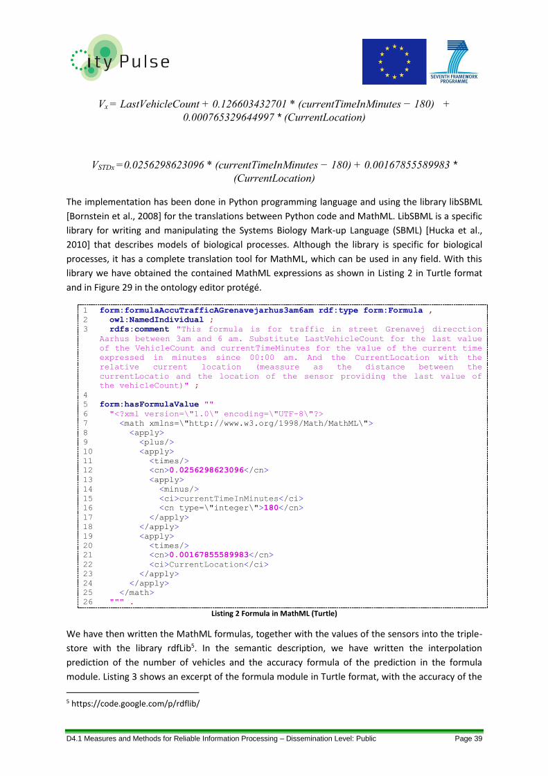
D4.1 Measures and Methods for Reliable Information Processing – Dissemination Level: Public Page 39
Vx = LastVehicleCount + 0.126603432701 * (currentTimeInMinutes − 180) +
0.000765329644997 * (CurrentLocation)
VSTDx =0.0256298623096 * (currentTimeInMinutes − 180) + 0.00167855589983 *
(CurrentLocation)
The implementation has been done in Python programming language and using the library libSBML
[Bornstein et al., 2008] for the translations between Python code and MathML. LibSBML is a specific
library for writing and manipulating the Systems Biology Mark-up Language (SBML) [Hucka et al.,
2010] that describes models of biological processes. Although the library is specific for biological
processes, it has a complete translation tool for MathML, which can be used in any field. With this
library we have obtained the contained MathML expressions as shown in Listing 2 in Turtle format
and in Figure 29 in the ontology editor protégé.
1 form:formulaAccuTrafficAGrenavejarhus3am6am rdf:type form:Formula ,
2 owl:NamedIndividual ;
3 rdfs:comment "This formula is for traffic in street Grenavej direcction
Aarhus between 3am and 6 am. Substitute LastVehicleCount for the last value
of the VehicleCount and currentTimeMinutes for the value of the current time
expressed in minutes since 00:00 am. And the CurrentLocation with the
relative current location (meassure as the distance between the
currentLocatio and the location of the sensor providing the last value of
the vehicleCount)" ;
4
5 form:hasFormulaValue ""
6 "<?xml version=\"1.0\" encoding=\"UTF-8\"?>
7 <math xmlns=\"http://www.w3.org/1998/Math/MathML\">
8 <apply>
9 <plus/>
10 <apply> 11 <times/> 12 <cn>0.0256298623096</cn> 13 <apply> 14 <minus/> 15 <ci>currentTimeInMinutes</ci> 16 <cn type=\"integer\">180</cn> 17 </apply> 18 </apply> 19 <apply> 20 <times/> 21 <cn>0.00167855589983</cn> 22 <ci>CurrentLocation</ci> 23 </apply> 24 </apply> 25 </math> 26 """ .
Listing 2 Formula in MathML (Turtle)
We have then written the MathML formulas, together with the values of the sensors into the triple-
store with the library rdfLib5. In the semantic description, we have written the interpolation
prediction of the number of vehicles and the accuracy formula of the prediction in the formula
module. Listing 3 shows an excerpt of the formula module in Turtle format, with the accuracy of the
5 https://code.google.com/p/rdflib/
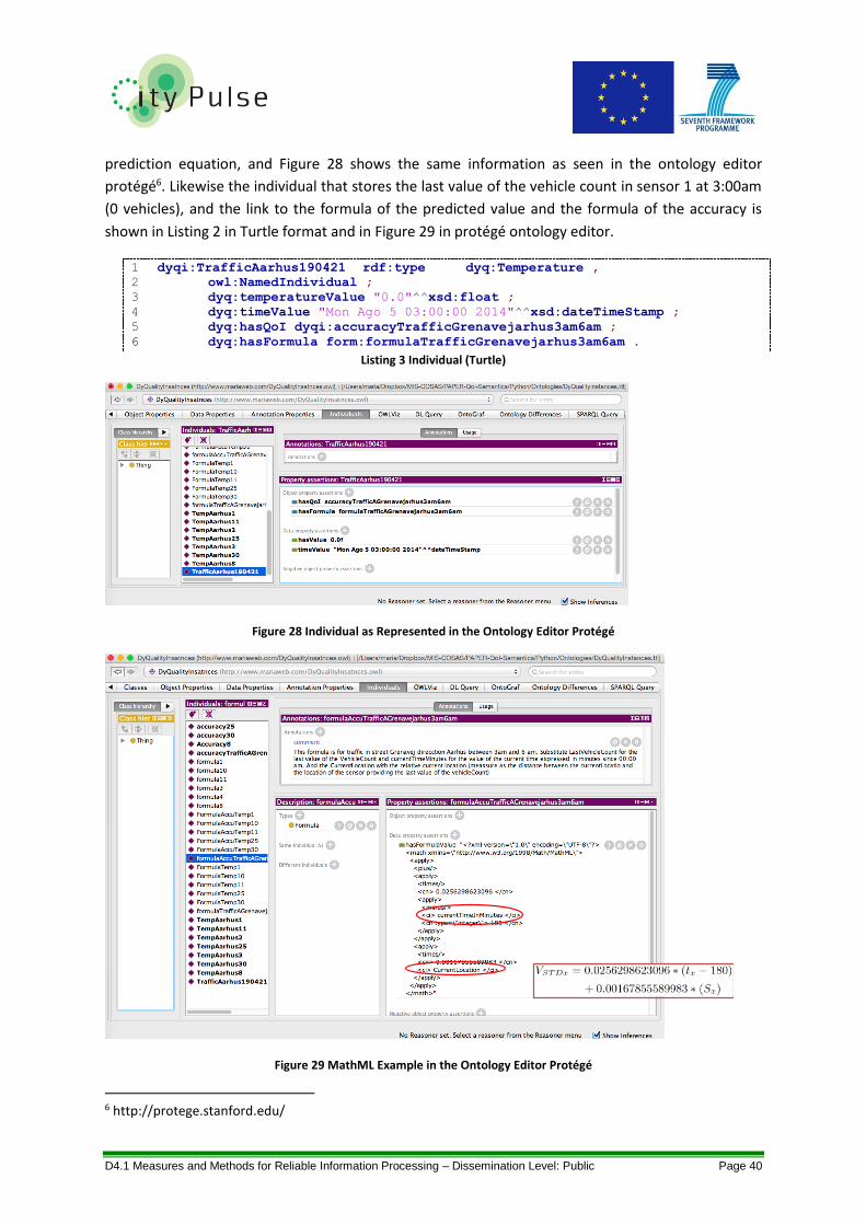
D4.1 Measures and Methods for Reliable Information Processing – Dissemination Level: Public Page 40
prediction equation, and Figure 28 shows the same information as seen in the ontology editor
protégé6. Likewise the individual that stores the last value of the vehicle count in sensor 1 at 3:00am
(0 vehicles), and the link to the formula of the predicted value and the formula of the accuracy is
shown in Listing 2 in Turtle format and in Figure 29 in protégé ontology editor.
1 dyqi:TrafficAarhus190421 rdf:type dyq:Temperature ,
2 owl:NamedIndividual ;
3 dyq:temperatureValue "0.0"^^xsd:float ;
4 dyq:timeValue "Mon Ago 5 03:00:00 2014"^^xsd:dateTimeStamp ;
5 dyq:hasQoI dyqi:accuracyTrafficGrenavejarhus3am6am ;
6 dyq:hasFormula form:formulaTrafficGrenavejarhus3am6am .
Listing 3 Individual (Turtle)
Figure 28 Individual as Represented in the Ontology Editor Protégé
Figure 29 MathML Example in the Ontology Editor Protégé
6 http://protege.stanford.edu/
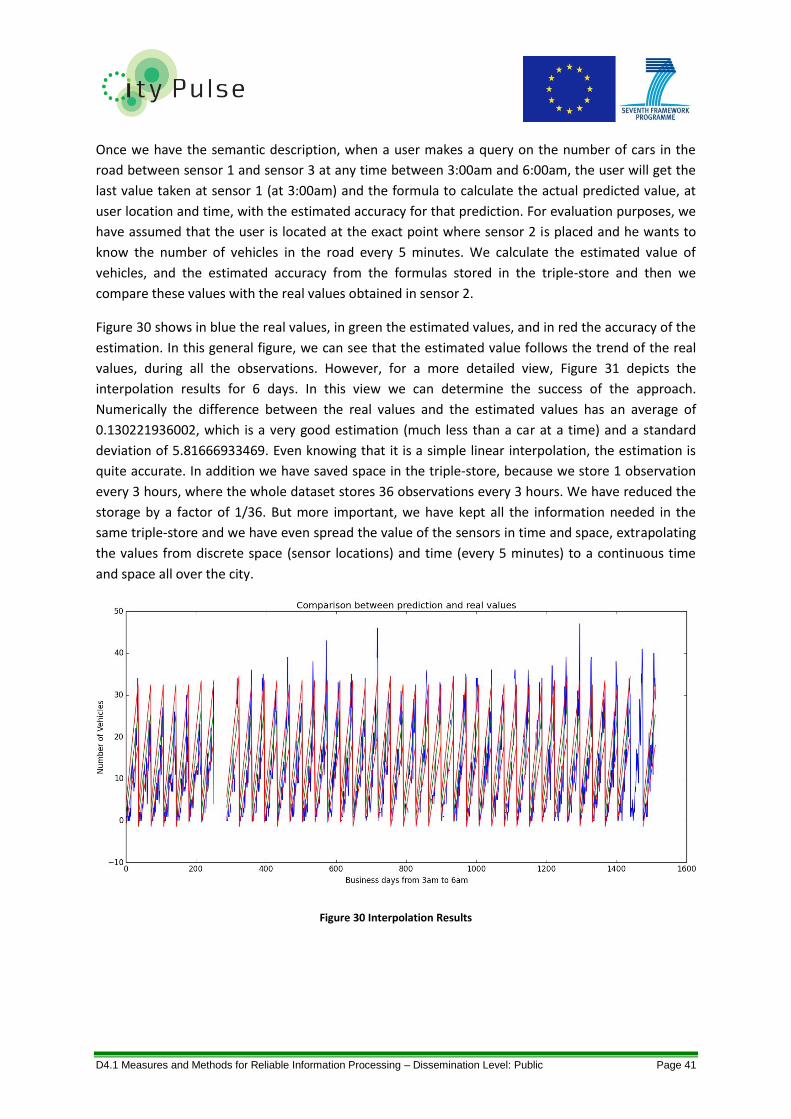
D4.1 Measures and Methods for Reliable Information Processing – Dissemination Level: Public Page 41
Once we have the semantic description, when a user makes a query on the number of cars in the
road between sensor 1 and sensor 3 at any time between 3:00am and 6:00am, the user will get the
last value taken at sensor 1 (at 3:00am) and the formula to calculate the actual predicted value, at
user location and time, with the estimated accuracy for that prediction. For evaluation purposes, we
have assumed that the user is located at the exact point where sensor 2 is placed and he wants to
know the number of vehicles in the road every 5 minutes. We calculate the estimated value of
vehicles, and the estimated accuracy from the formulas stored in the triple-store and then we
compare these values with the real values obtained in sensor 2.
Figure 30 shows in blue the real values, in green the estimated values, and in red the accuracy of the
estimation. In this general figure, we can see that the estimated value follows the trend of the real
values, during all the observations. However, for a more detailed view, Figure 31 depicts the
interpolation results for 6 days. In this view we can determine the success of the approach.
Numerically the difference between the real values and the estimated values has an average of
0.130221936002, which is a very good estimation (much less than a car at a time) and a standard
deviation of 5.81666933469. Even knowing that it is a simple linear interpolation, the estimation is
quite accurate. In addition we have saved space in the triple-store, because we store 1 observation
every 3 hours, where the whole dataset stores 36 observations every 3 hours. We have reduced the
storage by a factor of 1/36. But more important, we have kept all the information needed in the
same triple-store and we have even spread the value of the sensors in time and space, extrapolating
the values from discrete space (sensor locations) and time (every 5 minutes) to a continuous time
and space all over the city.
Figure 30 Interpolation Results

D4.1 Measures and Methods for Reliable Information Processing – Dissemination Level: Public Page 42
Figure 31 Interpolation Results (Zoom)
We have also performed a test under the supposition that even the same prediction model applies
for the 3 hours. We can access real data every hour. In this scenario, every hour we align the
estimation to the real value. The results, as shown in the zoomed view in Figure 32, are not
considerable better than the previous scenario, probably due to the nature of the dataset,
containing a great contribution of the high frequency component. However, this scenario shows the
possibility of adapting the estimations with real values as we get them, without the need to change
the estimation model (or estimation formula). This is an example of re-utilisation of formulas, and
the goodness of the linked data philosophy even if the data models are stored in the same machine.
Figure 32 Interpolation Results (Zoom / Sync Every Hour)
The previous scenarios show the feasibility of our proposal and open the path to new ways of
efficient use of semantic triple-stores with dynamic data. Although we are aware that traffic has fine

D4.1 Measures and Methods for Reliable Information Processing – Dissemination Level: Public Page 43
algorithms coming from the field of queue theory, our main purpose is not to improve any
algorithm. The simplicity of the used algorithm highlights the dynamicity of the semantics, which is
the final aim of this work. Furthermore, this generic algorithm can be implemented, even in the lack
of information, to apply other techniques (e.g. location of semaphores, or details on cross streets of
the city to apply queue theory techniques).
As a result of these experiments, we can conclude that dynamic semantics enhance the efficiency of
semantic descriptions by storing prediction models, instead of the whole raw data, levering the store
capacity of the triple-store and fasten the time response of queries. We have proved the feasibility
of our proposal with a simple prediction model, obtaining promising results.
5.6 Aggregation of Information Quality In the context of Smart City applications, data streams from different sources with different formats
may be implemented as event services and these services are federated or composed to answer
complex, coarse-grained event queries at real-time. The quality of query results may vary depending
on which and how the event services are used in the event service composition. Some quality
properties may propagate along the event service network. In Table 1 a list of quality metrics is
presented. In the following we elaborate a set of propagable quality metrics in event service
compositions and discuss the quality aggregation schema for these quality metrics. Using the
aggregation schema, we can calculate or estimate the quality of query results over federated data
streams.
5.6.1 Propagable Quality Metrics
We consider the following quality metrics are propagable in complex event services:
Accuracy
o Completeness describes the completeness of events delivered by an event service, it can be
numerically represented as recall rates in percentages, denoted C,
o Correctness describes the correctness of events delivered by an event service, it can be
numerically represented as precision in percentages, denoted Acc
Communication.
o Latency describes the delay in time for an event service, i.e., the temporal difference
between the time when the event consumer receives the notification and the time when the
event actually happens (usually denoted by the timestamp of the event), denoted L,
o Availability describes the possibility of an event service being accessible, it can be
numerically represented in percentages, denoted Ava,
Cost.
o Monetary_Consumption describes the monetary cost for an event service, denoted P,
o Energy_Consumption describes the energy cost for an event service, denoted E,
o Network_Consumption describes the usage of network bandwidth for an event service,
denoted B and

D4.1 Measures and Methods for Reliable Information Processing – Dissemination Level: Public Page 44
Security.
o Encryption describes the encryption protocol used by event services numerically
represented as integer security levels, higher numerical value indicate more secure and
complex encryption methods, denoted S.
Using the definition given above, a quality vector Q =< L, P, E, B, Ava, C, Acc, S> can be specified to indicate the performance of an event service in 8 dimensions.
5.6.2 Quality Aggregation
To calculate the overall quality of an event service composition, a quality aggregation schema is
required. The quality of an event service composition is affected by three factors: Service
Infrastructure, Composition Pattern, and Event Engine. The Service Infrastructure consists of
computational hardware, service Input/Output (I/O) implementation, and the physical network
connection. It determines the inherent I/O capability of a service. The Composition Pattern refers to
the local event patterns evaluated by the event engine. A composition pattern consists of a set of
member event services and a set of event operators connecting these event services. Indeed, the
performance varies on which services are used to produce the complex events and how event
operators correlate them. In this section four event operators are discussed: “And”, “Or”,
“Sequence”, and “Repetition”. A detailed definition of the operators is provided by Gao et al. [Gao et
al., 2014a]. The internal implementation of the Event Engine also has an impact on the event service
composition performance. However, it can be difficult to assess or specify, because it depends on
different implementations of event engines. Table 3 summarises how different quality parameters of
an event service composition are calculated based on the three factors.
Table 3 Overall Quality Calculation

D4.1 Measures and Methods for Reliable Information Processing – Dissemination Level: Public Page 45
Table 4 Quality Aggregation Rules Based on Composition Patterns
The Composition Pattern is a key factor in aggregating quality properties for event service compositions. Event patterns are represented as event syntax trees. In this report, a step-wise transformation of event syntax tree is adopted to aggregate quality properties. More specifically, we apply aggregation rules from the leaves to the roots on event syntax trees. Aggregation rules for different quality dimensions can be event operator dependent or independent. Event operator dependent rules are defined based on the quality properties of the set of Direct Sub-Trees (DSTs) of the entire event syntax trees. Event operator independent rules are defined based on the quality properties of the set of Immediately Composed Event services (ICEs). Table 4 shows the detailed rules for each quality dimension. In the following we explain the rationale for each rule.
1. Monetary and Energy Consumption are operator independent properties. They can be specified in different manners, e.g., price can be charged over subscription time or volume, similar for energy consumption. For simplicity we assume they are specified over time. Then the overall price or energy cost E is the sum of the price or energy cost of the immediately composed event services (denoted Eice).
2. Availability, Correctness and Encryption are operator independent properties. The correctness/availability of E is the product of event service correctness/availability in Eice; the security level is determined by the most vulnerable encryption method of the event service in Eice.
3. Latency of event E is an operator dependent property. It is determined by the last event completing the event pattern of E. Therefore, if the root operator of E is sequence or repetition, the latency of E is same as the last event in the direct sub events of E (denoted Edst). Otherwise, it is hard to predict when the last direct sub event occurs, therefore we make an approximation with the average of the latencies of the event services in Edst.
4. Completeness is an operator dependent property. The completeness of E can be estimated based on its direct sub event frequencies (denoted f(e), e ∈ Edst, for the estimation of f(e) see [Gao et al., 2014b]) and the completeness of direct-sub-events. The idea is to first derive the estimated receiving frequency of E based on the frequency and completeness of its direct-sub-events, and then divide the estimated receiving frequency by the theoretical frequency of E. For “Sequence”, “Repetiton” or “And” operators, the estimated receiving frequency of E is the minimum of the products of the sending frequency and completeness of the event services in Edst. On the contrary, for “Or” operators the maximum is used as the estimated receiving frequency.
5. Network Consumption can be measured by the number of events consumed by an event composition, i.e., its traffic demand. We refer readers to [Gao et al., 2014b] for detailed description on estimating traffic demands of event composition based on the frequencies of primitive events.

D4.1 Measures and Methods for Reliable Information Processing – Dissemination Level: Public Page 46
6. Conflict Resolution & Fault Recovery The CRFR component has the main objective to increase the stability of the system by providing
alternative solutions when the quality of the streams is modified (in most cases when the quality
drops). The reputation and QoI Evaluation system updates the stream quality through continuous
stream monitoring. Without the CRFR component the application (from CityPulse WP5 - Real-Time
IoT Intelligence) should directly retrigger the service composition component from WP3 (Large-Scale
IoT Stream Processing) in order to obtain an alternative combination of streams that fulfils the
application particular requirements (the request contains also the QoI/QoS constraints). In the smart
city context, it is highly probable that the stream QoI varies and a quality drop can happen for a
short period. As a result the retriggering step will be very frequent.
Instead of continuous retriggering of service composition the WP5 component can generate a fault
recovery request if the stream quality drops. Then the CRFR component will generate estimated
events and inject them in the data bus for a short period of time. After a period of time, if the stream
quality is not restored, the application should shift to another stream. In that case, the fault recovery
has the scope of generating the estimated data and the conflict resolution has to find alternative
streams. Emulated values are injected when a missing measurement is detected or if the measured
value is outside its range limit specified by the domain expert. Also this component considers the
trend of the measured values and if an abnormal behaviour is detected, it automatically generates
the estimation. This feature provides conflict resolution at data level.
The conflict resolution increases the stability by identifying alternative data sources. The
functionality is similar to the one provided by service composition component from WP3, only the
context is different. The service composition is triggered when the application starts or if it needs a
new combination of data sources. The conflict resolution should be triggered when the data source
quality drops. From the application point of view the result is the same, it receives a new set of
streams. Because of that, it would be redundant to have two components that fulfil the same task in
the framework. As a result of that, the research and development effort will be used in collaboration
with WP3 in order to improve the performance of the service composition component. We propose
to change the mechanism based on genetic algorithms with an answer set programming solution as
it is stated in the project description of work. This feature provides conflict resolution at stream
level. The results of this work will be documented in D4.2 Testing and fault recovery for Reliable
Information Processing.
The traffic datasets from the ODAA platform were used during the development and evaluation
stages of the conflict resolution and fault recovery components. As presented in Section 5.2, the
missing data percentage in the traffic dataset is about 8%. As a result of that, one role of the fault
recovery components is to provide missing value estimation for real-time and historic data.
In this section the fault recovery and its interaction with the other components of the framework is
presented. In addition, in the last section the algorithm used for traffic missing data estimation is
described.
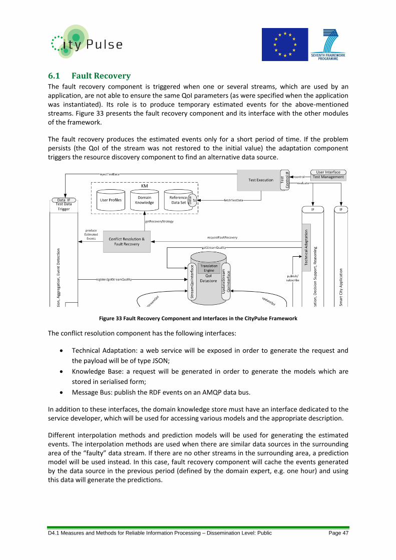
D4.1 Measures and Methods for Reliable Information Processing – Dissemination Level: Public Page 47
6.1 Fault Recovery The fault recovery component is triggered when one or several streams, which are used by an application, are not able to ensure the same QoI parameters (as were specified when the application was instantiated). Its role is to produce temporary estimated events for the above-mentioned streams. Figure 33 presents the fault recovery component and its interface with the other modules of the framework.
The fault recovery produces the estimated events only for a short period of time. If the problem persists (the QoI of the stream was not restored to the initial value) the adaptation component triggers the resource discovery component to find an alternative data source.
Figure 33 Fault Recovery Component and Interfaces in the CityPulse Framework
The conflict resolution component has the following interfaces:
Technical Adaptation: a web service will be exposed in order to generate the request and
the payload will be of type JSON;
Knowledge Base: a request will be generated in order to generate the models which are
stored in serialised form;
Message Bus: publish the RDF events on an AMQP data bus.
In addition to these interfaces, the domain knowledge store must have an interface dedicated to the service developer, which will be used for accessing various models and the appropriate description.
Different interpolation methods and prediction models will be used for generating the estimated events. The interpolation methods are used when there are similar data sources in the surrounding area of the “faulty” data stream. If there are no other streams in the surrounding area, a prediction model will be used instead. In this case, fault recovery component will cache the events generated by the data source in the previous period (defined by the domain expert, e.g. one hour) and using this data will generate the predictions.

D4.1 Measures and Methods for Reliable Information Processing – Dissemination Level: Public Page 48
6.2 Fault Recovery Workflow Figure 34 shows the fault recovery workflow. The technical adaptation component from WP5 is
responsible to turn on/off the fault recovery functionality. When a request is generated it has to
contain the ID of the data source for which estimated events have to be generated. Based on the ID,
the fault recovery component is able to identify the appropriate model, which has to be used.
Figure 34 Fault Recovery Workflow
6.3 Missing Values Estimation As presented in the state of the art section, mainly two types of methodologies can be used for
missing values estimation. The methodology based on interpolation is not feasible in case of traffic
data estimation, because the direct spatial distance between two sensors is not relevant. For
instance, we can have a small city where the sensor reports low traffic and nearby (or passing
through the city) we can have a motorway where high traffic is present. If one of the sensors from
the city fails to provide measurements, it is not feasible to combine the measurements coming from
the traffic sensors within the city and the traffic sensors from the motorway. In order to avoid this,
we propose to use a prediction model, which is able to forecast the traffic measurement when we
have missing data based on the previous valid measurements.
The solution proposed for traffic missing value estimation is based on k-NN (k-Nearest Neighbour)
algorithm [Aha et al., 1991]. We have considered that the reference dataset is composed by 𝑛
representative sequences of 𝑑 consecutive traffic measurements (the resulting dataset has the
size 𝑛 × 𝑑). If a missing value is detected, the algorithm uses the last 𝑑 − 1 measurements provided
by the sensor and compares them with the values form the first 𝑑 − 1 columns from the reference
dataset. More precisely, for each line of the dataset, the distance (using a distance metric) between
the values from the specific line and the last measurements is computed. At the end 𝑘 lines are
selected, which have the smallest distance. In conclusion the most relevant 𝑘 predictors are
selected. The values from column 𝑑 of the 𝑘 predictors are used to estimate the missing value
(simple or weighted average can be used to aggregate the value).
Figure 35 presents the general approach for missing traffic data estimation. The k-NN algorithm is
implemented by the traffic data estimator component. The latest traffic events are stored in a
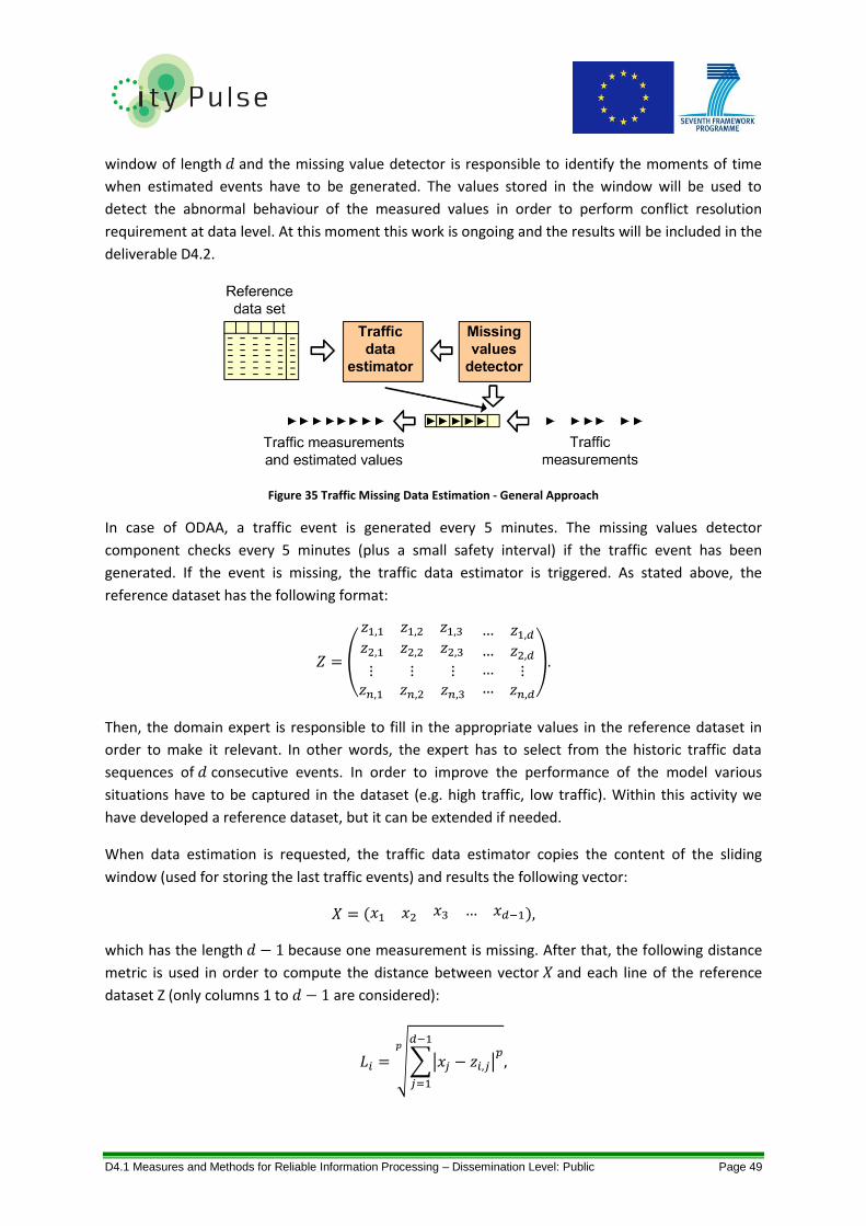
D4.1 Measures and Methods for Reliable Information Processing – Dissemination Level: Public Page 49
window of length 𝑑 and the missing value detector is responsible to identify the moments of time
when estimated events have to be generated. The values stored in the window will be used to
detect the abnormal behaviour of the measured values in order to perform conflict resolution
requirement at data level. At this moment this work is ongoing and the results will be included in the
deliverable D4.2.
Figure 35 Traffic Missing Data Estimation - General Approach
In case of ODAA, a traffic event is generated every 5 minutes. The missing values detector
component checks every 5 minutes (plus a small safety interval) if the traffic event has been
generated. If the event is missing, the traffic data estimator is triggered. As stated above, the
reference dataset has the following format:
𝑍 = (
𝑧1,1 𝑧1,2 𝑧1,3 … 𝑧1,𝑑𝑧2,1 𝑧2,2 𝑧2,3 … 𝑧2,𝑑
⋮𝑧𝑛,1
⋮𝑧𝑛,2
⋮𝑧𝑛,3
……
⋮𝑧𝑛,𝑑
).
Then, the domain expert is responsible to fill in the appropriate values in the reference dataset in
order to make it relevant. In other words, the expert has to select from the historic traffic data
sequences of 𝑑 consecutive events. In order to improve the performance of the model various
situations have to be captured in the dataset (e.g. high traffic, low traffic). Within this activity we
have developed a reference dataset, but it can be extended if needed.
When data estimation is requested, the traffic data estimator copies the content of the sliding
window (used for storing the last traffic events) and results the following vector:
𝑋 = (𝑥1 𝑥2 𝑥3 … 𝑥𝑑−1),
which has the length 𝑑 − 1 because one measurement is missing. After that, the following distance
metric is used in order to compute the distance between vector 𝑋 and each line of the reference
dataset Z (only columns 1 to 𝑑 − 1 are considered):
𝐿𝑖 = √∑|𝑥𝑗 − 𝑧𝑖,𝑗|𝑝
𝑑−1
𝑗=1
𝑝
,
D4.1 Measures and Methods for Reliable Information Processing – Dissemination Level: Public Page 50
where: 𝐿𝑖 denotes the distance between line 𝑖 of the reference dataset and the vector 𝑋 and 𝑝 ∈
{1,2,3} defines the type of the norm used (𝑝 = 2 represents the Euclidian distance).
At the end, the result of the following vector of distances will be as follows:
𝐿 = {𝐿1, 𝐿2, … , 𝐿𝑛}.
From the vector 𝐿 the 𝑘 smallest values are selected (their index indicates the lines from 𝑍), which
are very close to the current traffic situation which is represented by the vector 𝑋. The matrix N
contains the selected lines from the reference dataset as follows:
𝑁 = (
𝑎1,1 𝑎1,2 𝑎1,3 … 𝑎1,𝑑𝑎2,1 𝑎2,2 𝑎2,3 … 𝑎2,𝑑
⋮𝑎𝑘,1
⋮𝑎𝑘,2
⋮𝑎𝑘,3
⋱…
⋮𝑎𝑘,𝑑
),
where, 𝑎𝑖,𝑗 (𝑗 = 1. . 𝑑) represents the 𝑖th selected neighbour.
The estimated value is obtained using the following formula:
𝑒 = ∑𝑤𝑖𝑎𝑖,𝑑
∑ 𝑤𝑖,
𝑘
𝑖=1
where, 𝑤𝑖 is the weight of the neighbour 𝑖 which can be 1 or the inverse distance between line 𝑖 of
matrix 𝑁 (without the element on the column 𝑑) and vector 𝑋.
Another very similar approach is to consider the reference dataset and the vector 𝑋 as containing
the differences between the 𝑑 consecutive events. This method, as is demonstrated below, has
better results because it considers the trend (the variation of measured values).
In order to evaluate the performance of the model a test dataset was created, which follows the
same structure as Z. Each line of the matrix contains a sequence of 𝑑 − 1 elements, which are used
for computing the estimated value and the actual value. The KPI represent the maximum difference
between estimated value and the real value and it has to be as small as possible.
The traffic data estimator has been evaluated using the Aarhus traffic data from August and
September 2015. Figure 36 shows the error (tested with an independent test set) of the prediction
model. The first graph represents the situation when the actual traffic measurements are considered
and the second one for difference between consecutive events. For each situation the following
configurations have been considered:
Uniform L2: 𝑤𝑖 = 1 and 𝑝 = 2;
Weighted L1: 𝑤𝑖 = 1 𝑑𝑖𝑠𝑡𝑎𝑛𝑐𝑒⁄ and 𝑝 = 1;
Weighted L2: 𝑤𝑖 = 1 𝑑𝑖𝑠𝑡𝑎𝑛𝑐𝑒⁄ and 𝑝 = 2;
Weighted L3: 𝑤𝑖 = 1 𝑑𝑖𝑠𝑡𝑎𝑛𝑐𝑒⁄ and 𝑝 = 3.

D4.1 Measures and Methods for Reliable Information Processing – Dissemination Level: Public Page 51
Figure 36 Traffic Data Estimator Error
The resulting computation time for 𝑘 = 40 , 𝑛 = 4971 and 𝑑 = 10 is less than 0.7 seconds.
According to the graphs, the smallest error (less then 3 cars) has been obtained for the 𝑍 containing
the differences between consecutive events and weighted L2.

D4.1 Measures and Methods for Reliable Information Processing – Dissemination Level: Public Page 52
7. Implementation This section presents the implementation of the Reliable Information Processing in the CityPulse
framework. In the first part the individual components are introduced in the architecture context. In
the second part the basic workflow is shown.
7.1 Components/Architecture The Reliable Information Processing aims to ensure stable operation through the utilisation of
information sources with annotated QoI and reputation values. The annotation and conflict
resolution component supports other components of the CityPulse framework with handling data
sources of varying reliability.
The following paragraphs describe the individual components and their interaction. The architecture
of the components is illustrated in Figure 37.
Figure 37 Reliable Information Processing Architecture
Reputation & QoI Evaluation System
The Reputation & QoI Evaluation System is the central component for the active evaluation of QoI
for data sources and their steady adaption. This evaluation can either be triggered by events that are
sent by the monitoring components or the event management components of other CityPulse
framework modules. In contrast to monitoring components, divergences and conflicts can be found
in the long term. With additional historical data, it is possible to find correlations or contradictions in
various data sources to adapt the QoI and save them to the QoI Datastore. Furthermore the
Reputation & QoI Evaluation System
QoIDatastore
WP
3 V
irtu
alis
ati
on
, Fe
der
atio
n, A
ggre
gati
on
, Eve
nt
Det
ect
ion
WP
5 V
isu
aliz
atio
n, D
eci
sio
n S
up
po
rt, R
eas
on
ing
Eve
nt
Ma
nag
em
ent
updateStreamInformation publish/subscribe
getStreamQualityQ
oI N
oti
fica
tio
n
Inte
rfa
ce
Stre
amQ
oiIn
terf
ace
Qo
I No
tifi
cati
on
In
terf
ace
Up
dat
eSt
ream
Qo
iInte
rfa
ce
Ato
mic
M
on
ito
rin
g
Stre
am
Vir
tual
isa
tio
n
updateStreamInformation
Be
hav
iou
r A
sse
ssm
ent
IF
Co
rre
lati
on
M
on
ito
rin
g
updateStreamInformationanalyse
correlations
1..n
TranslationEngine
Mo
nito
rin
gIF
Event Management
register/getStreamQuality
Conflict Resolution & Fault Recovery
User ProfilesDomain
Knowledge
Tech
nic
al A
dap
tati
on
requestAdaptation
selectStreams
Ge Multi-Criteria RankingGetPreferences
getStreamQuality
Reference Data Set
KM
publish/subscribe

D4.1 Measures and Methods for Reliable Information Processing – Dissemination Level: Public Page 53
reputation based on the provenance of data sources is calculated to maintain the trustworthiness of
different data sources. Both the QoI and the reputation of a source are stored in the QoI Datastore.
QoI Datastore
The QoI Datastore stores QoI annotations of data streams. Components of the framework can
request specific information about data streams or use the publish/subscribe interface to receive
updates. On the fly translation to semantic annotation format ensures compatibility with various
representation systems. A Translation Engine is used to create required explicit QoI representation
(e.g. RDF) for related work packages.
Atomic Monitoring
The Atomic Monitoring is responsible for watching one single data stream for inconsistencies (e.g.
the frequency with the R&P algorithm). Additionally the Atomic Monitoring applies an incremental
time series analysis to the data streams to model an expected behaviour of the delivered
information. Due to the fact that the monitoring needs direct access to the data streams, it is placed
near the virtualisation of the stream.
Composite Monitoring
The Correlation Monitoring combines information of Atomic Monitoring components and watches
the abstract values that are delivered. Based on entity-, time- and geospatial- relationships the
different sources are aggregated and checked for plausibility. With the Correlation Monitoring it is
possible to detect faulty information sources within a group of data sources by comparison with
other group members. Composite Monitoring compares acquired data with comparable streams to
determine correlations and looks for divergences.
Conflict Resolution and Fault Recovery
The Conflict Resolution and Fault Recovery component is triggered if one or several streams, used by
an application, are not able to ensure the same QoI parameters (as were specified when the
application was instantiated). Its role is to temporary generate estimated events for the above
mentioned streams. Different interpolation methods and prediction models will be used for
generating the estimated events. The interpolation methods are used if there are similar data
sources in the surrounding area of the “faulty” data stream. If there are no other streams in the
surrounding area, a prediction model will be used instead. In this case the fault recovery component
will cache the events generated by the data source in the previous period (defined by the domain
expert, e.g. one hour) and using this data will generate the predictions.
Technical Adaptation
The fault recovery component generates the estimated events only for a short period of time. If the
problem persists (the QoI of the stream was not restored to the initial value), the adaptation
component triggers the resource discovery component to find an alternative data source.
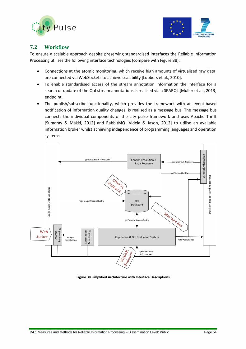
D4.1 Measures and Methods for Reliable Information Processing – Dissemination Level: Public Page 54
7.2 Workflow To ensure a scalable approach despite preserving standardised interfaces the Reliable Information
Processing utilises the following interface technologies (compare with Figure 38):
Connections at the atomic monitoring, which receive high amounts of virtualised raw data,
are connected via WebSockets to achieve scalability [Lubbers et al., 2010].
To enable standardised access of the stream annotation information the interface for a
search or update of the QoI stream annotations is realised via a SPARQL [Muller et al., 2013]
endpoint.
The publish/subscribe functionality, which provides the framework with an event-based
notification of information quality changes, is realised as a message bus. The message bus
connects the individual components of the city pulse framework and uses Apache Thrift
[Sumaray & Makki, 2012] and RabbitMQ [Videla & Jason, 2012] to utilise an available
information broker whilst achieving independence of programming languages and operation
systems.
Figure 38 Simplified Architecture with Interface Descriptions
Reputation & QoI Evaluation System
QoIDatastore
Larg
e S
cale
Dat
a A
nal
ysis
De
cisi
on
Su
pp
ort
an
d R
easo
nin
g
notifyQoIChange
getStreamQuality
Ato
mic
M
on
ito
rin
g
Co
rre
lati
on
M
on
ito
rin
g
analysecorrelations
updateStreamInformation
register/getStreamQuality
Conflict Resolution & Fault Recovery
Tech
nic
al A
dap
tati
on
requestFaultRecoverygenerateEstimatedEvents
get/updateStreamQuality

D4.1 Measures and Methods for Reliable Information Processing – Dissemination Level: Public Page 55
Figure 39 Sequence Diagram Stream Registration
An example for the registration of a data stream at the Reliable Information Processing component
is depicted in Figure 39. The Semantic Annotation subcomponent of the Large Scale Data Analysis,
which annotates new data streams, is responsible for the registration of new streams. For this
process a SPARQL endpoint is defined. A simple registration query is shown on the right side of
Figure 39. The registration query contains values for the different QoI metrics that should be fulfilled
by the stream. In the example the stream should always deliver right values and the resolution of
the delivered values should be at least 0.2.
Figure 40 Sequence Diagram Stream Information Update
The current QoI value is calculated by the Reputation & Quality Evaluation System and saved to the
QoI Datastore. Figure 40 illustrates the process of updating a data stream with new information
regarding the QoI of the stream. The update process can be started by different components:
Monitoring: the first possibility to update the stream information is by the internal
Monitoring component of the Reliable Information Processing. As introduced in Section 7.1,
the Monitoring is divided into the Atomic and the Correlation Monitoring. If the monitoring
determines that the frequency of a data steam deviates from the specified frequency,
annotated in the registration, the Evaluation System is notified via the
updateStreamInformation and can calculate a new QoI value for the data stream.
Semantic Annotation
QoI Datastore
registerStream()
PREFIX qoi: <http://ict-citypulse.eu/ontologies/StreamQuality/>INSERT DATA{ <http://quality/stream3124>
qoi:correctness 1;qoi:resolution 0.1;qoi:deviation 0.2;qoi:completeness 1;qoi:… .
}
Example Message
Event Management
QoI Datastore
updateStreamInformation()
Repuation & Quality Evaluation System
updateStreamQuality()
Semantic Annotation
updateStreamInformation()
updateStreamQuality()
Monitoring
updateStreamInformation()
updateStreamQuality()
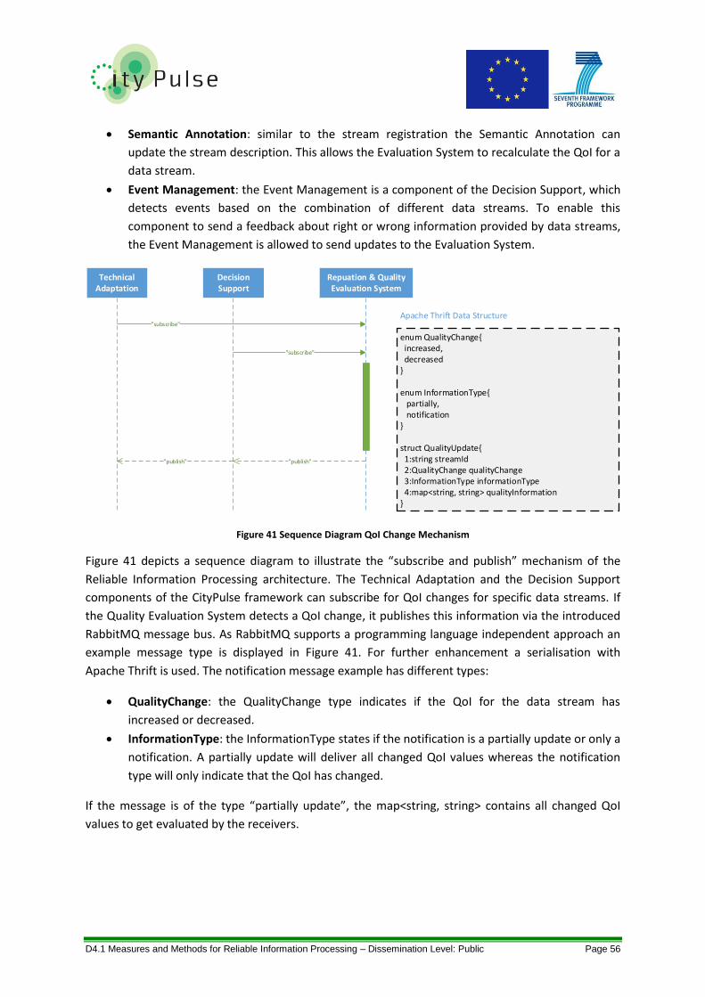
D4.1 Measures and Methods for Reliable Information Processing – Dissemination Level: Public Page 56
Semantic Annotation: similar to the stream registration the Semantic Annotation can
update the stream description. This allows the Evaluation System to recalculate the QoI for a
data stream.
Event Management: the Event Management is a component of the Decision Support, which
detects events based on the combination of different data streams. To enable this
component to send a feedback about right or wrong information provided by data streams,
the Event Management is allowed to send updates to the Evaluation System.
Figure 41 Sequence Diagram QoI Change Mechanism
Figure 41 depicts a sequence diagram to illustrate the “subscribe and publish” mechanism of the
Reliable Information Processing architecture. The Technical Adaptation and the Decision Support
components of the CityPulse framework can subscribe for QoI changes for specific data streams. If
the Quality Evaluation System detects a QoI change, it publishes this information via the introduced
RabbitMQ message bus. As RabbitMQ supports a programming language independent approach an
example message type is displayed in Figure 41. For further enhancement a serialisation with
Apache Thrift is used. The notification message example has different types:
QualityChange: the QualityChange type indicates if the QoI for the data stream has
increased or decreased.
InformationType: the InformationType states if the notification is a partially update or only a
notification. A partially update will deliver all changed QoI values whereas the notification
type will only indicate that the QoI has changed.
If the message is of the type “partially update”, the map<string, string> contains all changed QoI
values to get evaluated by the receivers.
Technical Adaptation
Repuation & Quality Evaluation System
"subscribe"
"subscribe"
Decision Support
"publish""publish"
enum QualityChange{ increased, decreased}
enum InformationType{ partially, notification}
struct QualityUpdate{ 1:string streamId 2:QualityChange qualityChange 3:InformationType informationType 4:map<string, string> qualityInformation}
Apache Thrift Data Structure

D4.1 Measures and Methods for Reliable Information Processing – Dissemination Level: Public Page 57
8. Conclusion and Outlook Smart cities are composed of frameworks that support a variety of applications, making use of
heterogeneous data sources. These data sources are coming mostly from IoT devices such as
sensors, smart phones, cameras and also citizen sensing data collected from social media. Evaluating
the quality of these sources is a mandatory process if reliable smart city applications should be
provided. Since in heterogeneous infrastructures there is no resilient ground-truth, which can be
assumed to be always correct, the comparison of multiple individual data sources can verify
reported events. To achieve high framework compatibility, the QoI provided by data streams has to
be determined in an objective and application independent way. A normalised QoI value enables
comparability and eases the stream selection. In the proposed Quality of Information approach
distinct measurable QoI metrics, like the frequency, are evaluated for every observation and
compared against the initial annotated metric.
The work presented in this deliverable shows that, dependent on the availability of individual data
sources, various algorithms and processes can be used to evaluate city infrastructure data. Therefore
spatio-temporal relations between events and continuous measurements are used to determine
dependencies, conformance and contradictions in the evaluated datasets. To overcome limitations
of classical methods, new approaches, like mutual information and Reward and Punishment, have
been utilised to evaluate available data streams.
These measure allow a continuous observation of the sensor performance over lifetime and ensures
reliable execution of applications, which are using them. Sensor readings are evaluated by
comparison against information sources gathering similar or correlated data. This aspect will
become more important in a Smart City scenario processing data not only from governmental
deployed sensor networks, but also utilising privately generated content, like social media feeds or
otherwise published data. Therefore a sophisticated provenance and trust management framework
will be evaluated. In this way faulty reports will receive a lower quality value and the corresponding
information sources can be identified and are likely to be ignored in a higher level. On the other
hand an information source is able to regain credibility by delivering conforming information. A
limitation of the automated approach reveals if two information sources publish contradictory data
without any other correlating information sources addressing the same events. In this case it is not
automated solvable, which information contains the defect. The current CityPulse QoI approach
cannot detect a high density of failing sensors, due to accessing information on a higher level
without having access to an entity/device management. These obstacles can be overcome by
employing a systematic sensor device monitoring throughout the heterogeneous, distributed
architectures. To gather more information about the quality, more and more data sources, like
application feedback streams, integration of global information brokers, and adapted mobile apps,
which assess consumed information sources, are needed in smart city infrastructures. Overall the
usage of an event ontology, which is describing the effects of incidents, will enable the modelling of
the mutual impact of various data streams.
D4.1 Measures and Methods for Reliable Information Processing – Dissemination Level: Public Page 58
9. References
Aha et al., 1991 Aha, D. W., Kibler, D., & Albert, M. K. (1991). Instance-based learning algorithms. Machine learning, 6(1), 37-66.
Anscombe, 1973 Anscombe, F. J. (1973). Graphs in statistical analysis. The American Statistician, 27(1), 17-21.
Asif et al., 2014 Asif, M. T., Dauwels, J., Goh, C. Y., Oran, A., Fathi, E., Xu, M., ... & Jaillet, P. (2014). Spatiotemporal patterns in large-scale traffic speed prediction. Intelligent Transportation Systems, IEEE Transactions on, 15(2), 794-804.
Baader et al., 2012 Baader, F., Ghilardi, S., & Lutz, C. (2012). LTL over description logic axioms. ACM Transactions on Computational Logic (TOCL), 13(3), 21.
Bar-Noy et al., 2011 Bar-Noy, A., Cirincione, G., Govindan, R., Krishnamurthy, S., LaPorta, T. F., Mohapatra, P., ... & Yener, A. (2011, March). Quality-of-information aware networking for tactical military networks. In Pervasive Computing and Communications Workshops (PERCOM Workshops), 2011 IEEE International Conference on (pp. 2-7). IEEE.
Barnaghi, 2014 Barnaghi, P. (2014). Dynamic Semantics for Dynamic IoT Environments. In Keynote 7th International Workshop on Semantic Sensor Networks in conjunction with the 13th International Semantic Web Conference (ISWC).
Benesty et al., 2008 Benesty, J., Chen, J., & Huang, Y. A. (2008). On the importance of the Pearson correlation coefficient in noise reduction. Audio, Speech, and Language Processing, IEEE Transactions on, 16(4), 757-765.
Bisdikian et al., 2009 Bisdikian, C., Kaplan, L. M., Srivastava, M. B., Thornley, D. J., Verma, D., & Young, R. I. (2009, July). Building principles for a quality of information specification for sensor information. In Information Fusion, 2009. FUSION'09. 12th International Conference on (pp. 1370-1377). IEEE.
Bisdikian et al., 2013 Bisdikian, C., Kaplan, L. M., & Srivastava, M. B. (2013). On the quality and value of information in sensor networks. ACM Transactions on Sensor Networks (TOSN), 9(4), 48.
Bizer et al., 2009 Bizer, C., Heath, T., & Berners-Lee, T. (2009). Linked data-the story so far. International journal on semantic web and information systems, 5(3), 1-22.
Bornstein et al., 2008 Bornstein, B. J., Keating, S. M., Jouraku, A., & Hucka, M. (2008). LibSBML: an API library for SBML. Bioinformatics, 24(6), 880-881.
Brayner et al., 2014 Brayner, A., Coelho, A. L., Marinho, K., Holanda, R., & Castro, W. (2014). On query processing in wireless sensor networks using classes of quality of queries. Information Fusion, 15, 44-55.
Bristow & Kennedy, 2013 Bristow, D. N., & Kennedy, C. A. (2013). Maximizing the use of energy in cities using an open systems network approach. Ecological Modelling, 250, 155-164.
Chen & Zhang, 2014 Li, L., Chen, X., & Zhang, L. (2014). Multimodel ensemble for freeway traffic state estimations. IEEE Transactions on Intelligent Transportation Systems, 15(3).
CityPulse-D2.2 Tsiatsis, V. et al. (2014, August). CityPulse D2.2 - Smart City Framework.
CityPulse-D3.1 Kolozali, S. et al. (2014, August). CityPulse D3.1 - Semantic Data Stream Annotation for Automated Processing.

D4.1 Measures and Methods for Reliable Information Processing – Dissemination Level: Public Page 59
Emaldi et al., 2013 Emaldi, M., Pena, O., Lázaro, J., Vanhecke, S., Mannens, E., & Lopez-de-Ipina, D. (2013). To trust, or not to trust: Highlighting the need for data provenance in mobile apps for smart cities. In Proceedings of the 3rd International Workshop on Information Management for Mobile Applications (pp. 68-71).
Frenay & Verleysen, 2014 Frénay, B., & Verleysen, M. (2014). Classification in the presence of label noise: a survey. Neural Networks and Learning Systems, IEEE Transactions on, 25(5), 845-869.
Ganeriwal et al., 2008 Ganeriwal, S., Balzano, L. K., & Srivastava, M. B. (2008). Reputation-based framework for high integrity sensor networks. ACM Transactions on Sensor Networks (TOSN), 4(3), 15.
Gao et al., 2014a Gao, F., Curry, E., Ali, M. I., Bhiri, S., & Mileo, A. (2014). QoS-aware Complex Event Service Composition and Optimization using Genetic Algorithms. In Service-Oriented Computing (pp. 386-393). Springer Berlin Heidelberg.
Gao et al., 2014b Gao, F., Curry, E., & Bhiri, S. (2014, May). Complex event service provision and composition based on event pattern matchmaking. In Proceedings of the 8th ACM International Conference on Distributed Event-Based Systems (pp. 71-82). ACM.
Gebser et al., 2011 Gebser, M., Kaufmann, B., Kaminski, R., Ostrowski, M., Schaub, T., & Schneider, M. (2011). Potassco: The Potsdam answer set solving collection. Ai Communications, 24(2), 107-124.
Haykin, 1998 Haykin, S. (1998). A Comprehensive Foundation. In Neural Networks, 2nd ed. Upper Saddle River, NJ, USA: Prentice Hall PTR.
Hossain et al, 2011 Hossain, M. A., Atrey, P. K., & Saddik, A. E. (2011). Modeling and assessing quality of information in multisensor multimedia monitoring systems. ACM Transactions on Multimedia Computing, Communications, and Applications (TOMM), 7(1), 3.
Hucka et al., 2010 Hucka, M., Bergmann, F. T., Hoops, S., Keating, S. M., Sahle, S., Schaff, J. C., ... & Wilkinson, D. J. (2010). The Systems Biology Markup Language (SBML): language specification for level 3 version 1 core. Nature proceedings
Iggena et al., 2014 Iggena, T., Kümper, D., & Tönjes, R. (2014). Kontinuierliche Bewertung von Informationsqualität in Stream-basierten Smart City Architekturen. ITG-Fachbericht-Mobilkommunikation–Technologien und Anwendungen.
Janowicz et al., 2013 Janowicz, K., Bröring, A., Stasch, C., Schade, S., Everding, T., & Llaves, A. (2013). A restful proxy and data model for linked sensor data. International Journal of Digital Earth, 6(3), 233-254.
Kasetty et al., 2008 Kasetty, S., Stafford, C., Walker, G. P., Wang, X., & Keogh, E. (2008, November). Real-time classification of streaming sensor data. In Tools with Artificial Intelligence, 2008. ICTAI'08. 20th IEEE International Conference on (Vol. 1, pp. 149-156). IEEE.
Keogh et al., 2003 Keogh, E., & Lin, J. (2005). Clustering of time-series subsequences is meaningless: implications for previous and future research. Knowledge and information systems, 8(2), 154-177.
Knott, 2000 Knott, G. D. (2000). Interpolating cubic splines (Vol. 18). Springer Science & Business Media.
Koller & Friedman, 2009 Koller, D., & Friedman, N. (2009). Probabilistic graphical models: principles and techniques. MIT press.
D4.1 Measures and Methods for Reliable Information Processing – Dissemination Level: Public Page 60
Kolozali et al., 2014 Kolozali, S., Bermudez-Edo, M., Puschmann, D., Ganz, F., & Barnaghi, P (2014). A Knowledge-based Approach for Real-Time IoT Data Stream Annotation and Processing. In IEEE International Conference on
Internet of Things (iThings).
Lathia et al., 2012 Lathia, N., Quercia, D., & Crowcroft, J. (2012). The hidden image of the city: sensing community well-being from urban mobility. In Pervasive computing (pp. 91-98). Springer Berlin Heidelberg.
Lopez et al., 1999 López, M. F., Gómez-Pérez, A., Sierra, J. P., & Sierra, A. P. (1999). Building a chemical ontology using methontology and the ontology design environment. IEEE intelligent Systems, 14(1), 37-46.
Lubbers et al., 2010 Lubbers, P., & Greco, F. (2010). Html5 web sockets: A quantum leap in scalability for the web. SOA World Magazine.
Malgady & Krebs, 1986 Malgady, R. G., & Krebs, D. E. (1986). Understanding correlation coefficients and regression. Physical therapy, 66(1), 110-120.
Mcardle et al., 2012 McArdle, G., Furey, E., Lawlor, A., & Pozdnoukhov, A. (2014). Using Digital Footprints for a City-Scale Traffic Simulation. ACM Transactions on Embedded Computing Systems 9, 4 (2012).
Mendez et al., 2013 Mendez, D., Labrador, M., & Ramachandran, K. (2013). Data interpolation for participatory sensing systems. Pervasive and Mobile Computing, 9(1), 132-148.
Muller et al., 2013 Müller, H., Cabral, L., Morshed, A., & Shu, Y. (2013). From RESTful to SPARQL: A Case Study on Generating Semantic Sensor Data. In SSN@ ISWC (pp. 51-66).
Jussien et al., 2008 Jussien, N., Rochart, G., & Lorca, X. (2008). Choco: an open source java constraint programming library. In CPAIOR'08 Workshop on Open-Source Software for Integer and Contraint Programming (OSSICP'08) (pp. 1-10).
Newman et al., 2006 Newman, M., Barabasi, A. L., & Watts, D. J. (Eds.). (2006). The structure and dynamics of networks. Princeton University Press.
Pautasso, 2014 Pautasso, C. (2014). RESTful web services: principles, patterns, emerging technologies. In Web Services Foundations (pp. 31-51). Springer New York.
Pham & Seow, 2013 Pham, M. T., & Seow, K. T. (2013, October). Multiagent Conflict Resolution Planning. In Proceedings of the 2013 IEEE International Conference on Systems, Man, and Cybernetics (pp. 297-302). IEEE Computer Society.
Quercia et al., 2012 Quercia, D., Séaghdha, D. Ó., & Crowcroft, J. (2012, May). Talk of the City: Our Tweets, Our Community Happiness. In ICWSM.
Ratti et al., 2010 Ratti, C., Sobolevsky, S., Calabrese, F., Andris, C., Reades, J., Martino, M., ... & Strogatz, S. H. (2010). Redrawing the map of Great Britain from a network of human interactions. PloS one, 5(12), e14248.
Rau & Fang, 2008 Rau, H., & Fang, Y. T. (2009, July). Conflict resolution of product package design for logistics using the triz method. In Machine Learning and Cybernetics, 2009 International Conference on (Vol. 5, pp. 2891-2896). IEEE.
Roth et al., 2011 Roth, C., Kang, S. M., Batty, M., & Barthélemy, M. (2011). Structure of urban movements: polycentric activity and entangled hierarchical flows. PloS one, 6(1), e15923.
Seni & Elder, 2010 Seni, G., & Elder, J. F. (2010). Ensemble methods in data mining: improving accuracy through combining predictions. Synthesis Lectures on Data Mining and Knowledge Discovery, 2(1), 1-126.
D4.1 Measures and Methods for Reliable Information Processing – Dissemination Level: Public Page 61
Scholkopf & Smola, 2002 Schölkopf, B., & Smola, A. J. (2002). Learning with kernels: Support vector machines, regularization, optimization, and beyond. MIT press.
Stein, 1999 Stein, M. L. (1999). Interpolation of spatial data: some theory for kriging. Springer Science & Business Media.
Strong et al., 1997 Strong, D. M., Lee, Y. W., & Wang, R. Y. (1997). Data quality in context. Communications of the ACM, 40(5), 103-110.
Stvilia et al., 2007 Stvilia, B., Gasser, L., Twidale, M. B., & Smith, L. C. (2007). A framework for information quality assessment. Journal of the American Society for Information Science and Technology, 58(12), 1720-1733.
Sumaray & Makki, 2012 Sumaray, A., & Makki, S. K. (2012, February). A comparison of data serialization formats for optimal efficiency on a mobile platform. In Proceedings of the 6th International Conference on Ubiquitous Information Management and Communication (p. 48). ACM.
Tchrakian et al., 2012 Tchrakian, T. T., Basu, B., & O'Mahony, M. (2012). Real-time traffic flow forecasting using spectral analysis. Intelligent Transportation Systems, IEEE Transactions on, 13(2), 519-526.
Turchi et al., 2014 Turchi, S., Paganelli, F., Bianchi, L., & Giuli, D. (2014, March). A lightweight linked data implementation for modeling the Web of Things. In Pervasive Computing and Communications Workshops (PERCOM Workshops), 2014 IEEE International Conference on (pp. 123-128). IEEE.
Videla & Jason, 2012 Videla, A., & Williams, J. J. (2012). RabbitMQ in action: distributed messaging for everyone. Manning.
Visintini et al., 2006 Visintini, A. L., Glover, W., Lygeros, J., & Maciejowski, J. (2006). Monte Carlo optimization for conflict resolution in air traffic control. Intelligent Transportation Systems, IEEE Transactions on, 7(4), 470-482.
Wang et al., 2008 Wang, W., Hou, J., Su, C., Liang, S., & Su, Y. (2008, October). Modeling on Conflict Resolution of Collaborative Design. In Wireless Communications, Networking and Mobile Computing, 2008. WiCOM'08. 4th International Conference on (pp. 1-4). IEEE.
Weisz & Steinberger, 2010 Weisz, H., & Steinberger, J. K. (2010). Reducing energy and material flows in cities. Current Opinion in Environmental Sustainability, 2(3), 185-192.
Williamson, 2011 Williamson, J. (2011). Mechanistic theories of causality part I. Philosophy Compass, 6(6), 421-432.
Yang & Wong, 2013 Yang, Y., & Wong, K. K. (2013). Spatial distribution of tourist flows to China's cities. Tourism Geographies, 15(2), 338-363.
Zheng et al., 2014 Zheng, Y., Capra, L., Wolfson, O., & Yang, H. (2014). Urban computing: concepts, methodologies, and applications. ACM Transactions on Intelligent Systems and Technology (TIST), 5(3), 38.
Zhou et al., 2014 Zhou, X., Shekhar, S., & Ali, R. Y. (2014). Spatiotemporal change footprint pattern discovery: an inter‐disciplinary survey. Wiley Interdisciplinary Reviews: Data Mining and Knowledge Discovery, 4(1), 1-23.