measures and metrics in uniform gravitational fields

7/29/2019 Measures and Metrics in Uniform Gravitational Fields

http://slidepdf.com/reader/full/measures-and-metrics-in-uniform-gravitational-fields 1/13

a r X i v : g

r - q c / 0 5 0 3 0 9 2 v 2 1 2 M a y 2 0 0 5

Measures and metrics in uniform gravitational fields∗

Marco AlbericiDipartimento di Fisica, Universita di Bologna Via Irnerio 46, 40126 Bologna, Italy .†

(Dated: February 7, 2008)

A partially alternative derivation of the expression for the time dilation effect in a uniform staticgravitational field is obtained by means of a thought experiment in which rates of clocks at rest atdifferent heights are compared using as reference a clock bound to a free falling reference system

(FFRS). Derivations along these lines have already been proposed, but generally introducing someshortcut in order to make the presentation elementary. The treatment is here exact: the clockswhose rates one wishes to compare are let to describe their world lines (Rindler’s hyperbolae) withrespect to the FFRS, and the result is obtained by comparing their lengths in space-time. Theexercise may nonetheless prove pedagogically instructive insofar as it shows that the some resultsof General Relativity (GR) can be obtained in terms of physical and geometrical reasoning withouthaving recourse to the general formalism. The corresponding GR metric is derived, to the purposeof making a comparison with solutions of Einstein field equation and with other metrics. For thisreasons this paper also compels to deal with a few subtle points inherent in the very foundations of GR.

I. INTRODUCTION

It is possible to show that the GR redshift formula for a uniform gravitational field ∆ ν/ν = gh/c2 it is an exactconsequence of the EP, and its derivation does not require GR formalism [2]. As is well known, this formula wasexperimentally verified for the first time in 1960 by Pound and Rebka [3]. The height difference (22.5m) used in theirexperiment was small compared to the gravitational field strength variations. For this reason their experiment hadthe purpose to verify only the first order effects predicted from GR that, for time dilation, bring to the above relation.In experiments involving stronger gravitational field variations it is necessary to use the exact Schwarzschild solutionof GR, and to take into consideration the earth rotation effects.

GR is a well-established theory, but it very often happens that its applications to some specific case involvessubtle points on which the agreement is not general: as a result, the conclusions of the analysis reported are oftennot univocal. This is the case, in particular, for the object of the present article, namely redshift in a uniformgravitational field. In Weinberg’s treatise [4], for instance, the gravitational redshift effect is thus commented: “For auniform gravitational field, this result could be derived directly from the Principle of Equivalence, without introducing

a metric or affine connection”. We have in fact already recalled that such derivations are possible and in an exact way[2]. Independently of this conclusion, one may always introduce transformations between reference frames at rest withrespect to the matter generating the field and FFRS which, in the case of a uniform field, are supposed to becomeextended, or global. The most natural way to describe such a transformation are Rindler hyperbolae. But Rindlerhimself [5], at the end of the paragraph of his book in which they are introduced and analysed, and after discussingthe fact that SR can deal in a proper way with accelerated frames, states: “A uniform gravitational field can not beconstructed by this method”. About 15 years ago, E.A. Desloge [6, 7, 8, 9], in a sequence of four articles, carried outa systematic investigation on uniformly accelerated frames and on their connection with gravitation. In agreementwith Rindler’s statement Desloge proved that there is no exact equivalence between a frame uniformly acceleratedand a frame at rest in a uniform gravitational fields [8]. By contrast, only three years later E. Fabri [10] derived theexpression of the time delay in a uniform gravitational field by explicit use of a FFRF, from which the world lines of objects at rest with the masses that generate the field are seen as Rindler hyperbolae. As far I know, there are notother papers approaching the problem in this way, except the Mould treatise [11]. The related metric is instead used

in important books and many paper (for example [12, 13]).In order to see whether a reconciliation between these apparently conflicting views can be obtained, I tried to setup an ideal experiment in which the rates of two standard clocks 1 sitting at different heights in a uniform and static

∗ This paper is the continuation of a previous work [1] of the same author and contains most part of it, but some definitions are different.From section III B different new calculations are added or modified and new results are derived; section V contains only new material.

†[email protected]; I.N.F.N. member, Sezione di Bologna.1 We will not come back here to the meaning to be attributed to expressions such as ‘Standard Clock’ or ‘Standard Rods’, as the question

has already been discussed in many books and papers and also in one of Desloge’s articles. We will just compare the proper time elapsed

http://arxiv.org/abs/gr-qc/0503092v2






























mailto:[email protected]

mailto:[email protected]




2

gravitational field are compared. The measuring process as seen from a FFRF, it is carefully analysed, followingthe approach based on Rindler hyperbolae. We will show that in this case the associated field it is not uniform if measured from an observer at rest with the FFRF, but that it appears to be uniform when its strength is measuredusing radar pulses generated and received from an observer at rest with the source generating the field. The metricderived with the approach based on Rindler hyperbolae (we will call it Rindler’s metric) is a solution of the Einsteinfield equation for the flat space (Rµνσρ = 0), and it is also the first order approximation of the Schwarzschild metric(section IV). At the end of the paper (section V) it will be proved that Desloge’s metric [8] (rigid FFRF describinga geodetic with uniform proper acceleration) can also be derived from an approach based on Rindler hyperbolae, but

with a different physical interpretation, that does not seems to be in agreement with the EP. For this reasons it isauthor opinion that, for uniform fields description, the Rindler’s metric it is the most useful one.

II. FREE-FALLING REFERENCE SYSTEMS

EP is the basic idea from which the bulk of GR theory was developed. In our applications we will not deal withcharged bodies and with non-gravitational forces in general. We are therefore entitled to overlook differences betweenweak and strong EP, differences that are present only when non-gravitational interactions are considered. We justconsider the EP in this form:

A body in free fall does not feel any acceleration, and behaves locally as an inertial reference system of SR.

We know that physical gravitational fields are not uniform, and there always exist tidal forces that oblige to consider

the validity of the EP only locally in space and time. The ideal case of a uniform and static field is however worthconsidering for its conceptual interest. In this ideal case FFRS, which in strictly physical situations are local inertialsystems, should become non-local.

EP invites to consider FFR systems the proper inertial systems. Let us then try to build a non-local FFRF,denoted as K , in a 2-dimensional space-time universe and study the world line of a particle at rest with the massesthat generate a uniform gravitational field g. Since this world line is considered with respect to the FFRF, we willassociate to the particle a (local) frame Σ−. It is easily proved [5] that the world line of a body falling along thevertical direction x with constant proper acceleration g is described by the hyperbola of equation:

x2 − c2t2 =c4

g2. (1)

Since we are considering acceleration with respect to K , it is material points at rest in Σ− that will describe anhyperbola of Eq. (1) in the Minkowski space-time of K (with an acceleration pointing in the direction opposite togravity). On the other hand, the observer sitting in Σ− will see material points at rest in K describe more complicatedworld lines. They have been explicitly calculated [14], and turn out indeed to be very different from those describedby Eq. (1) (on the same subject see [15]). Fortunately we do not need to deal with them in order to solve our problem.Proper acceleration g (acceleration relative to instantaneous rest frame) can be measured from an observer at rest withthe FFRF in x0 or from an observer at rest with Σ−. At time t = 0 the two observers have the same instantaneouslocal rest frame and they measure the same local acceleration g (an observer in Σ measures a force acting on him,while one in FFRF deduces its value from Σ trajectory).

In the following x will be called ‘coordinate position’ and t ‘coordinate time’, in order to distinguish them fromproper coordinate and proper time measured by Σ−. As usual c is the speed of light, but for sake of simplicity in thefollowing we will adopt units with c = 1. The space coordinate at time t = 0 is x0 = 1/g, so that Eq. (1) becomes

x2 − t2 = x20. (2)

It is now necessary to require that the radar distance between observers sitting at different height does not dependon proper time. By this request one find that a second RF Σ+ which, at t = 0, lies higher with respect Σ− by theamount h as measured by K , must be described by the following hyperbola [5]

x2 − t2 = (x0 + h)2, (3)

in the two RF.



3

were now the acceleration g depend on the coordinate. We will use g− to denote the acceleration in x0 and g+ thatin x0 + h 2

g+ =1

x0 + hg− =

1

x0, (5)

The fact that the acceleration depends on the coordinate value, seems to contradict the supposed uniformity of thefield. Nevertheless on this problem G.’t Hooft[16] wrote: “The gravitational field strength felt locally . . . is inverselyproportional to distance . . . . Even tough our field is constant in the transverse direction and with time, it decrease

with height”. We will discuss again this fact in subsection IIIC, but it worth now to underline that requiring the sameacceleration in Σ− and Σ+ generates unsolvable problems. One should in fact identify Σ+ with a spatial translationof Σ−:

(x − h)2 − t2 = x20, (6)

but in this case the radar distance between the two hyperbolae is not constant. There exist also paradoxical situations,

FIG. 1: Light ray emitted from Σ− in P ∗ will never reach Σ+

as that exhibited in Fig. 1, where Σ− cannot send a light signal that reaches Σ+. From this fact one should arguethat it is not possible to treat a uniform gravitational fields with an extended FFRF. But before giving up we willfully investigate physical properties of extended frames which see Σ+ and Σ− describing Rindler hyperbolae of Eq. (2)and Eq. (3). We will call such frames Rindler FFRF (and Rindler’s field those generating such kind of free fall). Thiskind of FFRF is the only one that satisfy three important physical experimentally verified conditions:

(1) Local acceleration does not depend on time;

(2) The ratio between proper time intervals at different altitudes is also constant in time (possibly depending onthe frames altitude), otherwise a Pound and Rebka-like experiment would give every day a different result;

(3) Radar distance between two observers located at a different height is a constant quantity which is time inde-pendent (it will as well possibly depend on the altitude).

Property (1) is surely satisfied because it is the basis used for deriving Rindler motion equation [5]. Property (2) and(3) were verified by Desloge [7] during the analysis of a uniform accelerated frame (described with Rindler hyperbolae).In the next subsection we will prove them in a way that appear to be more intuitive and probably more pedagogical.

A. Lorentz invariance

We required the FFRF to be extended as in SR, therefore it must satisfy Lorentz invariance. For proving it, let usapply a boost Λ of velocity v = arcthθ along x direction to the hyperbola parametric equation [5, 11, 18] describing

2 It is easily proven that g− and g+ are in the following relation:

g+ =g−

1 + g−h. (4)



4

Σ−

Λ =

cosh θ − sinh θ

− sinh θ cosh θ

x = x0 cosh gτ

t = x0 sinh gτ . (7)

The transformed hyperbola

x′ = x0 cosh(gτ

−θ)

t′ = x0 sinh(gτ − θ) , (8)

shows that the only effect of a Lorentz boost is a shift in the proper time origin ∆ τ = −θ/g.The application of Lorentz boosts on hyperbolae leaves their shape invariant and brings on the x axis all events

having the same velocity v = arcthθ. This proves Lorentz invariance of Rindler FFRF and shows that, for every givencoordinate velocity V = x/t (straight lines through the origin) there exist a Rindler FFRF in which the events onthis line are simultaneous.

B. Proper time intervals

We need to calculate the proper time interval along a world line between two generic coordinate times t1 and t2and using units with c = 1 we have the usual expression τ 12 = t2t1

√ 1

−V 2dt. Differentiating Eq. (2) or Eq. (3) one

obtains V = t/x and using Eq. (2) and Eq. (3) in order to eliminate x, we can calculate the proper time interval τ −

along the lower and τ + along the upper hyperbola

τ −12 =

t−2

t−1

1 1 + ( t

x0)2

dt = x0

t−2x0

t−

1x0

1 1 + y2

dy (9)

τ +12 =

t+2

t+1

1 1 + ( t

x0+h )2dt = (x0 + h)

t+2

x0+h

t+1

x0+h

1 1 + y2

dy. (10)

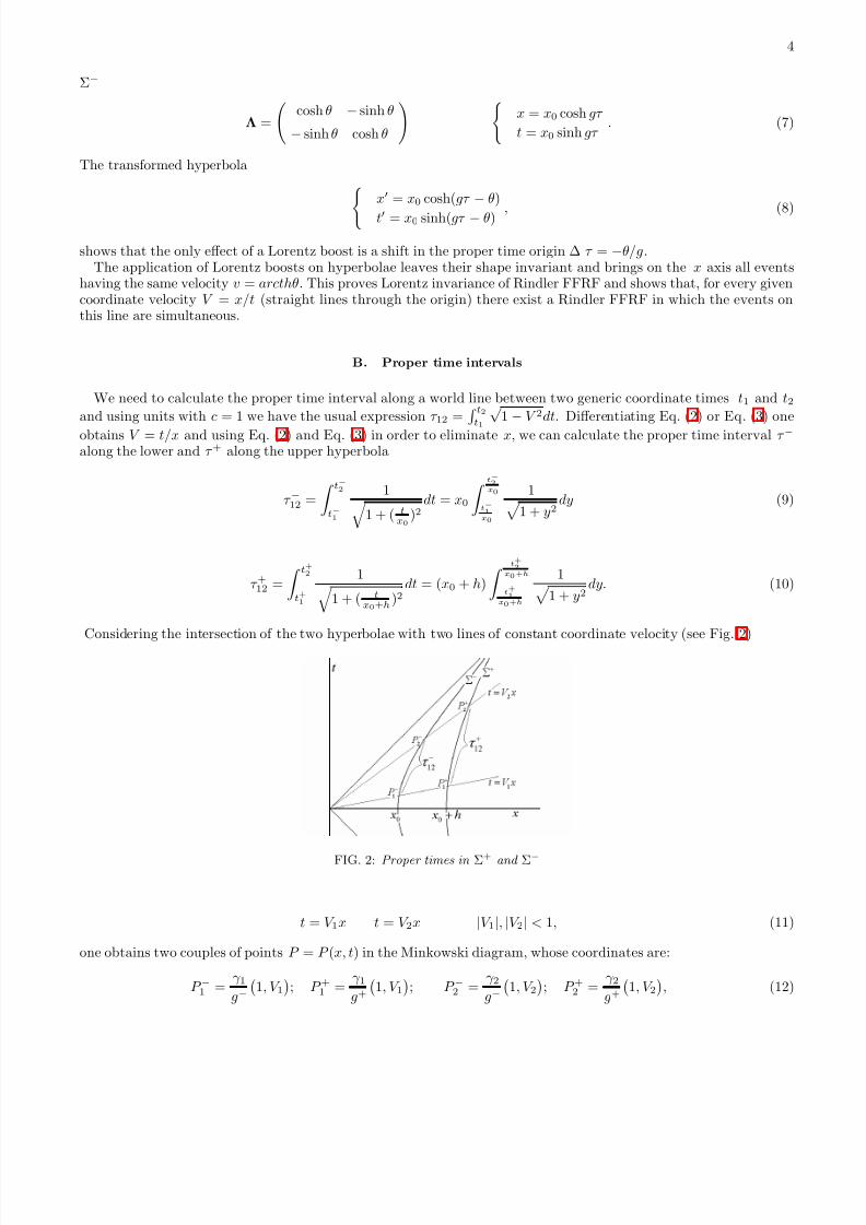
Considering the intersection of the two hyperbolae with two lines of constant coordinate velocity (see Fig. 2)

FIG. 2: Proper times in Σ+ and Σ−

t = V 1x t = V 2x |V 1|, |V 2| < 1, (11)

one obtains two couples of points P = P (x, t) in the Minkowski diagram, whose coordinates are:

P −1 =γ 1g−

1, V 1

; P +1 =γ 1g+

1, V 1

; P −2 =γ 2g−

1, V 2

; P +2 =γ 2g+

1, V 2

, (12)



6

Light rays through a couple of events with the same coordinate velocity laying on two Rindler hyperbolae,intersect other Rindler hyperbolae in a couple of points that have in turn the same coordinate velocity .

This property it is an extra bonus, as we did not request it in our premise at the beginning of section II, and it willmake it easier to perform clock rate comparison in an operational way. Using Lorentz transformation we proved thatall events having the same coordinate velocity admit a Rindler FFRF in which they are simultaneous. As a result of the above calculations, this appear now more clear, when one imagines two observers in Σ− and in Σ+ exchanginglight signals.

We can now calculate the proper time τ −S

elapsed in Σ− when a light ray covers the distance necessary to go fromΣ− to Σ+ and the proper time τ −R taken for the return trip:

τ −S =

t−2

t−V

1 1 + ( t

x0)2

dt = x0

t−2x0

t−

V x0

1 1 + y2

dy; τ −R =

t−V

t−1

1 1 + ( t

x0)2

dt = x0

t−V x0

t−

1x0

1 1 + y2

dy. (23)

The calculation leads to constant quantities 3

h− = τ −S = τ −R = x0 lnx0 + h

x0=

1

g−ln (1 + g−h). (24)

Calculation of proper times relative to an observer at rest with Σ+ leads also to an equal and constant time, whose

value is in this case:

h+ = τ +S = τ +R = (x0 + h) lnx0 + h

x0=

1

g+ln (1 + g−h). (25)

This is an important result that, differently from Desloge [7], we got by direct calculation:

The proper time, as measured by an observer on a Rindler hyperbola, taken by a light pulse to reach another Rindler hyperbola is equal to the proper time taken for the return trip, and this proper time is constant.

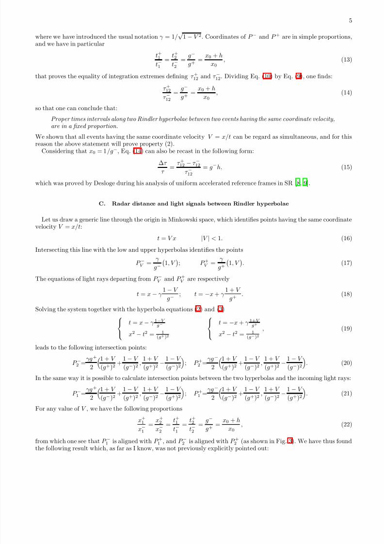
With the proof of this property, we completely fulfilled request (3) of section II.In Eq. (24) and Eq. (25) we calculated the proper time elapsed in Σ− and Σ+ for sending and receiving a light

ray. Multiplying this time by the speed of light (c = 1 in our units) we have radar distances (we used h− for radardistance measured by Σ− and h+ for that measured by Σ+).

FIG. 3: Light signal between two hyperbolae

3 If we tried instead to calculate the coordinate t time elapsed during the trip between Σ− and Σ+, we would find the following expression

t = γ h(2x0+h)x0+h

, which is not constant due to its dependence on γ .



7

III. PHYSICAL MEASUREMENTS

A. Clock delay

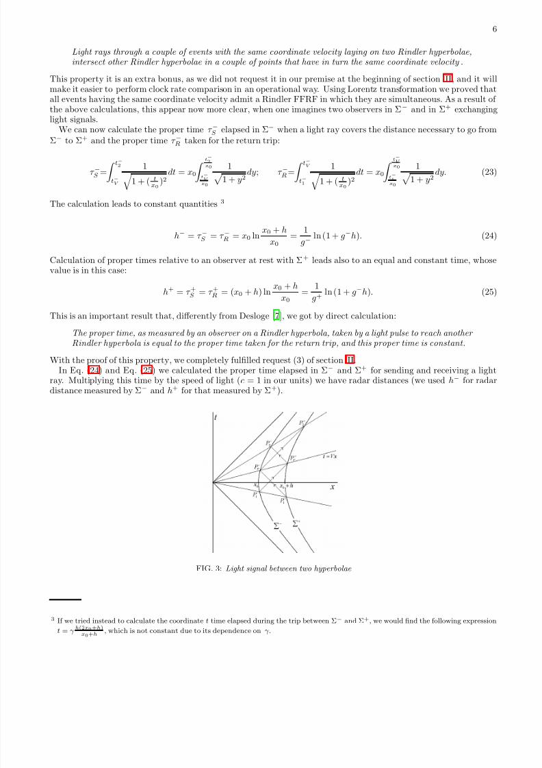
All necessary physical requirements having thus been satisfied, we feel entitled to set up a thought experimentin which two identically constructed clocks sit at rest, in a uniform and static gravitational field, at fixed distancesalong a field line of force. As has become customary, we will give a name to the physicists involved in the measuringprocesses; let’s say that Alice enjoys her life staying at rest with Σ− and Bob staying higher in Σ+. They will perform

a measure in the following way (see Fig. 4):

FIG. 4: Alice and Bob compare their clock rate

a) at time tS 1 Alice sends a light signal upwards;

b) at time t+1 Alice’s light pulse is received by Bob. When Bob receives the signal he starts his clock and immediatelysends back downwards a return light signal;

c) at time tR1 Alice receives the return signal from Bob. Adopting Einstein clock synchronization, she will arguethat Bob clock started at the intermediate time between sending and receiving the light pulse. According to her

clock this time is τ −1 = τ

−

S1+τ

−

R12 , and corresponds to coordinate time t1. In the previous section we saw that,

with respect to the origin, this event is aligned with the event in which Bob started his clock;

d) at time tS 2 Alice sends a light signal upwards;

e) at time t+2 Alice light pulse is received by Bob. When Bob receives the signal he stops his clock and immediatelysends back to Alice a return signal, in which the information of the proper time elapsed in Bob’s clock is stored;

f) at time tR2 Alice receives the return signal from Bob. She will argue that Bob clock had stopped at the intermediate

time between sending and receiving the light pulse. According to her clock this time is τ −2 =τ −S2+τ −

R2

2 whichcorrespond to coordinate time t2. We have again that in the Minkowski space-time of K , this event is alignedwith the origin and the event in which Bob stopped his clock.

The necessary measurements have thus been done, and Alice can compare her time with Bob’s. It is immediately seenthat any dependence on starting and stopping times cancels out, and that she will be able to compare two proper

times seen under the same angle centered in the origin: τ −

12 = τ −

2 − τ −

1 ; τ +12 = τ +2 − τ +1 . These proper times satisfyEq. (14) and Alice concludes4

∆τ

τ =

τ +12 − τ −12τ −12

= g−h. (26)

4 The experiment could be also done by sending starting and stopping signals from Σ+. In this case Bob would draw the very sameconclusion as Alice and they would both agree on the fact that Bob’s clock is faster than Alice’s. It worth stressing that this situationis different from that arising in SR with respect the time dilation effect, which is observed in a symmetric way by the two observers.



8

This fact was proved by Desloge [9] for uniform accelerated frames, but without having recourse to an ideal experimentas performed in this paper . It is also possible to compare Bob’s proper time τ +12 with Alice’s calculated either betweenthe two emission or reception events. This would not make any difference, because in both cases we would have onlyadded to and then subtracted from τ −12 the same quantity (the times taken by the outward and return trips given byτ −S = τ −R = x0 ln (1 + g−h)).

B. Space dilation

Solving Eq. (24) and Eq. (25) for h one gets

h = x0(eg−h− − 1) = x0(eg+h+ − 1), (27)

which makes it possible to rewrite the time dilation formula using local radar coordinates:

τ +

τ −= 1 + g−h = eg−h− = eg+h+, (28)

result pointed out from Desloge [9], in the case of uniform accelerated frames. It is also interesting to prove this resultfollowing redshift derivations based on potential energy loss of a quantum particle [10, 19, 20] 5.

One can prove that Eq. (28) is consistent with the following general result of GR [21],

ν +ν −

= eφ(x0+h)−φ(x0), (30)

which expresses the redshift in terms of the Newtonian potential φ of the gravitational field. Indeed, calculating thepotential difference we find:

φ(x0 + h) − φ(x0) =

x0+h

x0

g(x)dx = lnx0 + h

x0= ln(1 + g−h) (31)

which, inserted in Eq. (30), reproduces the time dilation formula (28). For a uniform gravitational field Desloge [9]

proved instead the expression ν +

ν − = egh, formally equivalent to Eq. (28) but here the gravitational acceleration is thesame for top and bottom observers and the distance is measured from a FFRF. Its derivation is based on the followingmetric [9]:

ds2 = e2ghdt2 − dh2, (32)

that is obtained requiring the FFRF to be rigid with its parts moving on geodetics with constant acceleration.Desloge’s metric of Eq. (32) is associated to a curved space with non vanishing Riemann tensor (Rxttx = g2e2gh)and Ricci tensor (Rtt = g2e2gx, Rxx = −g2) thus, for the Einstein field equation, the associated space is not empty.Because of the curvature associated to this metric, it is also not possible to have an extended FFRF. In the nextsection we will see that Eq. (28) is instead consistent with the metric derived from Einstein equation requiring thespace to be flat (Rµνσρ = 0) [15].

For a better understanding of space dilation it is useful to calculate it as measured with radar methods. Consideringthe ratio between Eq. (24) and Eq. (25) we get the following expression analog to time dilation:

h+

h−=

x0 + h

x0=

g−

g+. (33)

5 Let us imagine a particle of mass m0 falling from Σ+ to Σ−. From the FFRF’s viewpoint, the falling mass will arrive at Σ− with totalenergy E − = m0(1 + g−h). Once in Σ−, the particle transforms into a photon ‘climbing’ to Σ+. The related emitted frequency (inunit with hplank = 1) is ν e = m0(1 + g−h) while (for the conservation law) the received frequency in Σ+must be again ν r = m0. Asexpected, the frequency ratio is:

ν e/ν r = 1 + g−h = eg+h+ = eg

−h−. (29)

Using Eq.(4) it easy to show that also an observer comoving with the FFRF in x0 + h gets the same expression. If an observer sittingΣ+ and Σ+ used the same calculation procedure, he would instead find a wrong expression (ν e/ν r = 1 + g−h− = 1 + g+h+).



9

From this relation one find that the work per unit mass it is the same for observers in Σ− and Σ+ (g−h− = g+h+).It is also interesting to calculate the expression of the infinitesimal distance measured with radar methods by two

observers at rest with the field at different heights. We will use dh−x for denoting radar measurements of an infinitesimallength located at coordinate x, performed by an observer sitting in Σ−, and dh+x if the observer is located at Σ+. Astraightforward calculation, at first order, gives:

dh−

x = x0

ln

x + dh

x0− ln

x

x0

≈ x0

xdh; dh+x = (x0 + h)

ln

x + dh

x0− ln

x

x0

≈ x0 + h

xdh, (34)

whose ratio is:

dh+xdh−x

=x0 + h

x0=

g−

g+, (35)

from which one sees also that Σ− and Σ+ measure the same infinitesimal work per unit mass: dφ = g+dh+ = g−dh−.

C. Gravitational acceleration

In this subsection, we want to compare physical measurements performed by different observers in the same localframe. Let us consider two different measurements in Bob’s frame (Σ+):

1 Bob (Σ+) performs direct measurements with clocks and rods built in Σ−

2 Alice (Σ−) observes Bob’s frame by sending and receiving reflected light pulses.

The two measurements are in the following relations

dh−x0+h Alice′s measure

=g+

g−dh+

x0+h Bob′s measure

; dτ −x0+h Alice′s measure

=g+

g−dτ +x0+h

Bob′s measure

. (36)

Therefore, for the same couple of events, Alice obtains the same average velocity measured by Bob, but measuringshorter space and time intervals. Because of these contractions, it easy to prove that Alice will measure largeraccelerations than those measured by Bob:

gx0+h

Alice′

s measure

=g−

g+gx0+h

Bob′

s measure

. (37)

We know that the value of the gravitational acceleration obtained by Bob is g+ and, from Eq. (37), we learn thatAlice will find that the gravitational acceleration in Bob’s frame is g−. It is easy to conclude that:

Every observer sitting at rest with the source of gravity in a Rindler field finds that the gravitational acceleration has the same value everywhere.

For a more exact treatment we will now calculate the position of a body at rest with the FFRF as seen by radarmeasurements from an observer located in Σ−. One must calculate the proper time needed to go (or come back) fromΣ− to a fixed coordinate distance h∗ as a function of the intermediate proper time τ = τ S+τ R

2 (that we proved to bethe time elapsed in Σ− to arrive at the point of intersection with the straight line t = V x through P ∗, as shown inFig. 5). It is possible to verify that Σ− proper time is

τ − =x0

2ln

1 + V

1 − V . (38)

Inverting this relation (or directly from Eq. (7)), using g for denoting g−, and τ for τ −, one finds

V = tanh gτ . (39)

Using Eq. (12) one finds that at t = 0 the x coordinate of the hyperbola passing for P = (x0 + h∗, t∗) is x0 + h =(x0 + h∗)

√ 1 − V 2. Putting this value in Eq. (24), one can calculate the radar distance hrad from Σ− of a body falling

from the initial coordinate h∗ as a function of the coordinate velocity V :

hrad(V ) = x0 ln (1 + gh∗) +x02

ln(1 − V 2), (40)



10

and, using Eq. (39) to eliminate V , one gets the following motion equation:

hrad(τ ) = hrad(0) − x0 ln(cosh gτ ). (41)

Deriving with respect to Σ− proper time τ , one finds the corresponding velocity vrad(τ ) = − tanh gτ which has thesame value and opposite direction of the coordinate velocity V (τ ) and does not depend on the starting point of thefall h∗, but only on Σ− acceleration g = 1/x0. For this reason, an observer at rest with the field observes every partof the FFRF to move at the same speed.

One can also calculate the acceleration arad(τ ) =

−g cosh−2 gτ , whose value does not depend on h∗. For τ = 0 we

have arad(0) = −g and this confirms the fact (qualitatively discussed above) that, from the viewpoint of an observersitting in Σ−, the field under examination appears to be spatially uniform. In contrast, a falling body does not appearto move with an uniform proper acceleration, because τ it is not the proper time of the observed falling body. Thesame reasoning applies to an observer located in Σ+, but he observes everywhere a uniform acceleration with a smallerintensity g+.

It is also interesting to note another peculiarity of the Rindler’s field: moving along the x direction in a infi-nite Rindler’s field, the local gravitational acceleration g will assume every possible value. This has an importantconsequence:

All infinite extended Rindler’s fields are equivalent.

This seems a strange conclusion, but remember that our starting point was purely ideal, and we did not analysewhether and how such a field could be realized in the real world. However, some papers [22, 23] discusses a possibleconnection of the Rindler’s metric (which is found as a particular case of the Taub metric) with the study of theexterior solution of a planar symmetry mass distribution. If this will be confirmed, one would find that the fieldstrength would not depend on the mass value, and that the field would not vanish even with a vanishing mass.Desloge’s metric of Eq. (32) is instead not compatible with a planar mass distribution as, because of the Einstein fieldequation, it is associated to an non-empty space even out of the plane. As far as I know, most of the considerationspresented in this sections have not benn pointed out before.

IV. METRIC PROPERTIES

In section III we calculated the time ratio between two clocks at rest with the field τ τ 0

= 1 + gx, where now, in

order to denote the height measured from a FFRF (which starts the fall at t = 0) we use x instead of h, and g insteadof g−. Since the field we consider here is static, it is possible to write the metric in diagonal form

ds2 = A(x)dt2

−B(x)dx2. (42)

Writing the proper time elapsed for a clock at rest with the field dτ =

A(x)dt, comparing dτ with dτ 0 is easy toprove that the explicit expression of the first metric term is A(x) = (1 + gx)2. In order to find that of B(x), it ispossible to relate radar distances expressed using the metric coefficients with that we calculated in Eq. (24). One hasto solve the equation

A(0)

x

0

B(k)

A(k)dk =

1

glog(1 + gx). (43)

FIG. 5: Radar measure of a free falling body performed by Σ−



11

Setting A(x) = 1 + gx and differentiating one finds: B(x)

1 + gx=

1

1 + gx, (44)

hence B(x) = 1. The above result can also be deduced using the general flat space solutions of the Einstein fieldequation (imposing the condition Rµνσρ = 0). Rohrlich was the first to show that in this case we have the followingrelation between the metric coefficients [15]

B(x) =1

gd

dx

A(x)

2(45)

and, for A(x) = (1 + gx)2, we find again B(x) = 1. The resulting metric line element

ds2 = (1 + gx)2dt2 − dx2 (46)

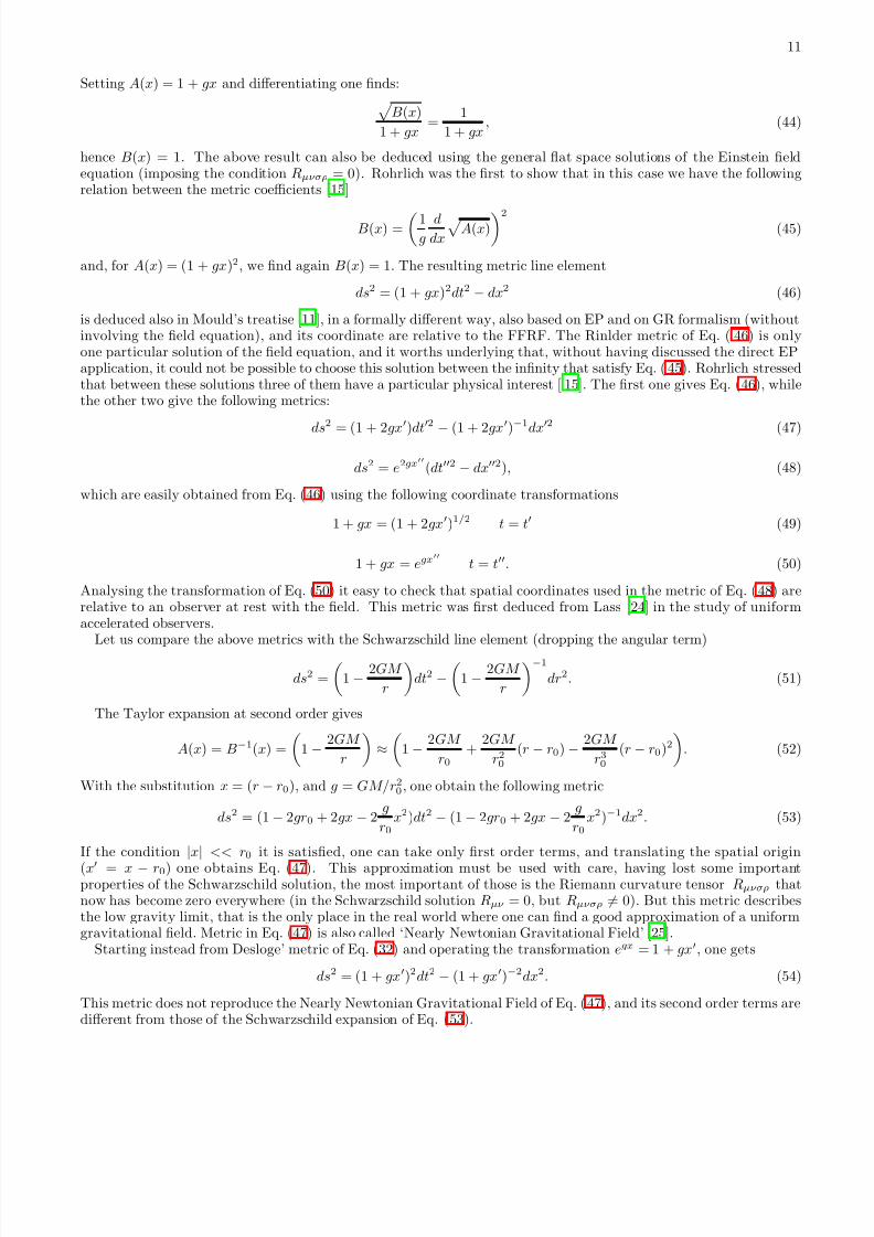
is deduced also in Mould’s treatise [11], in a formally different way, also based on EP and on GR formalism (withoutinvolving the field equation), and its coordinate are relative to the FFRF. The Rinlder metric of Eq. ( 46) is onlyone particular solution of the field equation, and it worths underlying that, without having discussed the direct EPapplication, it could not be possible to choose this solution between the infinity that satisfy Eq. ( 45). Rohrlich stressedthat between these solutions three of them have a particular physical interest [ 15]. The first one gives Eq. (46), whilethe other two give the following metrics:

ds

2

= (1 + 2gx

′

)dt

′2

− (1 + 2gx

′

)

−1

dx

′2

(47)

ds2 = e2gx′′(dt′′2 − dx′′2), (48)

which are easily obtained from Eq. (46) using the following coordinate transformations

1 + gx = (1 + 2gx′)1/2 t = t′ (49)

1 + gx = egx′′ t = t′′. (50)

Analysing the transformation of Eq. (50) it easy to check that spatial coordinates used in the metric of Eq. (48) arerelative to an observer at rest with the field. This metric was first deduced from Lass [24] in the study of uniformaccelerated observers.

Let us compare the above metrics with the Schwarzschild line element (dropping the angular term)

ds2 =

1 − 2GM

r

dt2 −

1 − 2GM

r

−1

dr2. (51)

The Taylor expansion at second order gives

A(x) = B−1(x) =

1 − 2GM

r

≈

1 − 2GM

r0+

2GM

r20(r − r0) − 2GM

r30(r − r0)2

. (52)

With the substitution x = (r − r0), and g = GM/r20, one obtain the following metric

ds2 = (1 − 2gr0 + 2gx − 2g

r0x2)dt2 − (1 − 2gr0 + 2gx − 2

g

r0x2)−1dx2. (53)

If the condition

|x

|<< r0 it is satisfied, one can take only first order terms, and translating the spatial origin

(x′

= x − r0) one obtains Eq. (47). This approximation must be used with care, having lost some importantproperties of the Schwarzschild solution, the most important of those is the Riemann curvature tensor Rµνσρ thatnow has become zero everywhere (in the Schwarzschild solution Rµν = 0, but Rµνσρ = 0). But this metric describesthe low gravity limit, that is the only place in the real world where one can find a good approximation of a uniformgravitational field. Metric in Eq. (47) is also called ‘Nearly Newtonian Gravitational Field’ [25].

Starting instead from Desloge’ metric of Eq. (32) and operating the transformation egx = 1 + gx′, one gets

ds2 = (1 + gx′)2dt2 − (1 + gx′)−2dx2. (54)

This metric does not reproduce the Nearly Newtonian Gravitational Field of Eq. (47), and its second order terms aredifferent from those of the Schwarzschild expansion of Eq. (53).



12

V. A DERIVATION OF DESLOGE’S METRIC

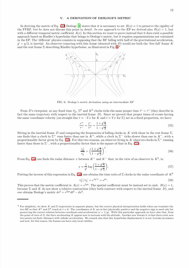
In deriving the metric of Eq. (32) Desloge [8] states that it is necessary to set B(x) = 1 to preserve the rigidity of the FFRF, but he does not discuss this point in detail. In our approach to the EP we derived also B(x) = 1, butwith a different temporal metric coefficient A(x). In this section we want to prove instead that it does exist a possibleapproach based on Rindler’s hyperbolae that brings to Desloge’s metric, but it requires argumentations not containedin the EP. The ‘different’ physics consists in supposing that the RF falling with half of the gravitational acceleration,g′ = g/2, is inertial. An observer comoving with this frame (denoted with D) would see both the ‘free fall’ frame K

and the rest frame Σ describing Rindler hyperbolae, as illustrated in Fig. 6 6

FIG. 6: Desloge’s metric derivation using an intermediate RF

From D’s viewpoint, at any fixed time t∗D, Σ0 and K 0 clocks ticks the same proper time t∗ = τ ∗ (they describe infact the same trajectory with respect to the inertial frame D). Since we proved that proper times of events havingthe same coordinate velocity (on straight line t = −V x for K and t = V x for Σ) are in a fixed proportion, we have:

τ +

τ −=

t−

t+=

1 + g′ h2

1 − g′ h2

. (55)

Sitting in the inertial frame D and comparing the frequencies of falling clocks in K with those in the rest frame Σ,one finds that a clock in Σ+ runs faster than one in K +, while a clock in Σ− ticks slower than one in K −, with a

proportionality factor given by Eq. (55). For this two reasons, an observer living in K observes clocks in Σ+

runningfaster than those in Σ−, with a proportionality factor that is the square of that in Eq. (55):

τ +Στ −Σ

=

1 + g′ h

2

1 − g′ h2

2

. (56)

From Eq. (24) one finds the radar distance x between K + and K − that, in the view of an observer in K 0, is:

x =1

g′log

1 + g′ h

2

1 − g′ h2

. (57)

Putting the inverse of this expression in Eq. (56) one obtains the time ratio of Σ clocks in the radar coordinate of K 0

τ +Σ /τ −Σ = e2g′x = egx. (58)

This proves that the metric coefficient is A(x) = e2gx. The spatial coefficient must be instead set to unit, B(x) = 1,

because Σ and K do not show a relative contraction (they both contract with respect to the inertial frame D), andone obtains Desloge’s metric ds2 = e2gxdt2 − dx2.

6 For simplicity, we drew K and Σ trajectories in separate planes, but the correct physical interpretation holds when one translate thetwo RF so that K 0 and Σ0 touch at t = 0. The coordinates of K are in fact physically positive and the negative sign is used only forpreserving the correct relation between coordinate and acceleration (x = 1/g). With this particular approach we have also that, fromthe point of view of D, the force accelerating K appear now to increase with the altitude. Another new feature it is that there exist nowtwo points (at finite distance) with infinite acceleration. We remark also that this hyperbolae displacement it is not Lorentz invarianceand now, for this reason, the frames can have only local validity.



13

VI. CONCLUDING REMARKS

As far I know, part of the analysis presented here is new, and hopefully could give some further physical insight onthe problems at hand. My first intent in writing this paper was mainly pedagogical. For this reason I have alwaystried to use simple mathematics, and sometimes calculations are perhaps not performed in the shortest way.

We conclude the discussion with some general considerations. In the physical case of central Newtonian potentialsit always exists an asymptotic limit in which gravity vanishes, from where one can imagine to let the fall of theFFRF start. This is used in GR to choose the correct form of Schwarzschild metric, but unfortunately this cannot be

achieved in the case of uniform fields. Supposing the fall of an extended body to start from within a region in whichthe field does not vanish, and taking into account the fact that the light speed limit is valid for every signal, one findslarge differences depending on the way the body is released. For example, starting the body fall removing a supportfrom its bottom, one has a ‘dilation’ effect, because the top starts to fall later than the bottom, whereas releasingthe hook from which it hangs, the falling body will experience a ‘contraction’ during the fall. Rindler FFRF leadsto a different rule: the fall starts simultaneously with respect to every local frame and it is ‘programmed’ to havethe same velocity along lines through the origin; observers at rest with the field will consider events on these linessimultaneous. Some of these points are discussed in detail in Mould treatise [11]. Incidentally, with this choice, wehave found that the FFRF measure gravity acceleration decreasing with height and this generate an asymptotic limitwhere gravity vanishes. Unfortunately, this limit does not have a non-relativistic (Newtonian) known counterpart, asit is in the case of Schwarzschild solution. But because the Rindler’s field is globally flat, one is free to choose theorigin x0 where he like and to compare the acceleration with the Newtonian one.

Acknowledgments

I am very grateful to Silvio Bergia who suggested me to study uniform gravitational field using only accelerated freefalling frames. He gave me also moral support and useful suggestions during the preparation of this work. Stimulatingdiscussions with Corrado Appignani, Luca Fabbri, Mattia Luzzi and Fabio Toscano are also gratefully acknowledged.

[1] M. Alberici, ‘Clock rate comparison in a uniform gravitational field’ , arXiv:gr-qc/0409033.[2] H.E. Price, ‘Gravitational Red-Shift Formula’ , Am. J. Phys. 42 (4), 336-339 (1974).[3] R.V. Pound and G.A. Rebka Jr., ‘Apparent Weight of Photons’ , Phys. Rev. Lett. 4 (7), 337-341 (1960).[4] Steven Weinberg, ‘Gravitation and Cosmology: Principles and Applications of the General Theory of Relativity’ , (John

Wiley and Sons New York 1972), first ed., pp. 80.[5] Wolfang Rindler, ‘Essential Relativity’ , (Springer Verlag New York 1992), 2nd ed., pp. 49-51.[6] Edward A. Desloge and R.J. Philpott, ‘Uniformly accelerated reference frames in special relativity’ , Am. J. Phys. 55 (3),

252-261 (1987).[7] Edward A. Desloge, ‘Spatial geometry in a uniformly accelerating reference frame’ , Am. J. Phys. 57 (7), 598-602 (1989).[8] Edward A. Desloge, ‘Nonequivalence of a uniformly accelerating reference frame and a frame at rest in a uniform gravita-

tional field’ , Am. J. Phys. 57 (12), 1121-1125 (1989).[9] Edward A. Desloge, ‘The gravitational red shift in a uniform field’ , Am. J. Phys. 58 (9), 856-858 (1990).

[10] E. Fabri, ‘Paradoxes of gravitational redshift’ , Eur. J. Phys. 15, 197-203 (1994).[11] Richard A. Mould, ‘Basic Relativity’ , (Springer New York 1994), first ed., pp.221-224[12] C.W. Misner, K.S. Thorne, J.A. Wheeler, ‘Gravitation’ , (Freeman and Company San Francisco 1973), first ed., pp. 173.[13] M. Pauri, M. Vallisneri, ‘Classical roots of the Unruh and Hawking effects’ , Found. Phys. 29, 1499-1520 (1999).[14] J. Dwayne Hamilton,‘The uniformly accelerated reference frame’ , Am. J. Phys. 46 (1), 83-89 (1978).[15] F. Rohrlich, ‘The Principle of Equivalence’ , Ann. Phys. 22, 169-191 (1963).[16] G. ’t Hooft, ‘Introduction to general relativity’ , http://www.phys.uu.nl∼thooft/lectures/genrel.pdf pp. 11[17] Wolfang Rindler,‘Kruskal Space and the Uniformly Accelerated Frame’ , Am. J. Phys. 34 (1), 1174-1178 (1966).[18] C.W. Misner, K.S. Thorne, J.A. Wheeler, ‘Gravitation’ , (Freeman and Company San Francisco 1973), first ed., pp. 167-176.[19] C.W. Misner, K.S. Thorne, J.A. Wheeler, ‘Gravitation’ , (Freeman and Company San Francisco 1973), first ed., pp. 187.[20] Bernard F. Schutz, ‘A First Course of General Relativity’ , (Cambridge University Press New York 1986), 1st. ed., pp. 118.[21] Wolfang Rindler, ‘Essential Relativity’ , (Springer Verlag New York 1992), 2nd ed., pp. 118.[22] R.M. Avakyan, E.V. Chubaryan, A.H. Yeranyan, ‘Homogeneous Gravitational Field in GR’ arXiv:gr-qc/0102030[23] A.F.F. Teixeira, ‘Taub, Rindler, and the static plate ’ arXiv:gr-qc/0502013[24] Harry Lass, ‘Accelerating Frames of Reference and the Clock Paradox’ , Am. J. Phys 31 (4), 274-276 (1963).[25] C.W. Misner, K.S. Thorne, J.A. Wheeler, ‘Gravitation’ , (Freeman and Company San Francisco 1973), first ed., pp. 445-446.

http://arxiv.org/abs/gr-qc/0409033






measures and metrics in uniform gravitational fields

Documents