measuring and exploiting the impact of exhibition...
TRANSCRIPT
Measuring and Exploiting the Impact
of Exhibition Scheduling on Museum Attendance
Victor Martınez-de-Albeniz∗ Ana Valdivia†
Submitted: May 17, 2016. Revised: October 10, 2017
Abstract
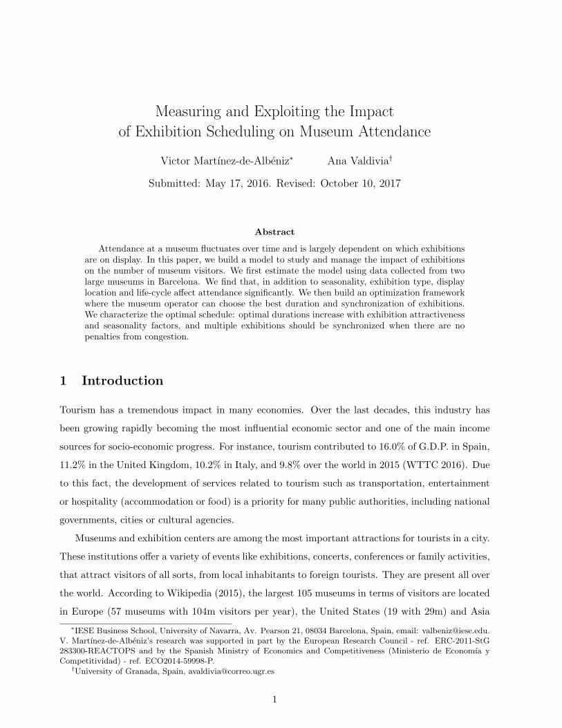
Attendance at a museum fluctuates over time and is largely dependent on which exhibitionsare on display. In this paper, we build a model to study and manage the impact of exhibitionson the number of museum visitors. We first estimate the model using data collected from twolarge museums in Barcelona. We find that, in addition to seasonality, exhibition type, displaylocation and life-cycle affect attendance significantly. We then build an optimization frameworkwhere the museum operator can choose the best duration and synchronization of exhibitions.We characterize the optimal schedule: optimal durations increase with exhibition attractivenessand seasonality factors, and multiple exhibitions should be synchronized when there are nopenalties from congestion.
1 Introduction
Tourism has a tremendous impact in many economies. Over the last decades, this industry has
been growing rapidly becoming the most influential economic sector and one of the main income
sources for socio-economic progress. For instance, tourism contributed to 16.0% of G.D.P. in Spain,
11.2% in the United Kingdom, 10.2% in Italy, and 9.8% over the world in 2015 (WTTC 2016). Due
to this fact, the development of services related to tourism such as transportation, entertainment
or hospitality (accommodation or food) is a priority for many public authorities, including national
governments, cities or cultural agencies.
Museums and exhibition centers are among the most important attractions for tourists in a city.
These institutions offer a variety of events like exhibitions, concerts, conferences or family activities,
that attract visitors of all sorts, from local inhabitants to foreign tourists. They are present all over
the world. According to Wikipedia (2015), the largest 105 museums in terms of visitors are located
in Europe (57 museums with 104m visitors per year), the United States (19 with 29m) and Asia
∗IESE Business School, University of Navarra, Av. Pearson 21, 08034 Barcelona, Spain, email: [email protected]. Martınez-de-Albeniz’s research was supported in part by the European Research Council - ref. ERC-2011-StG283300-REACTOPS and by the Spanish Ministry of Economics and Competitiveness (Ministerio de Economıa yCompetitividad) - ref. ECO2014-59998-P.
†University of Granada, Spain, [email protected]
1

(11 with 21m). The most visited and famous museums are superstars (Frey 1998), icons in their
respective cities (The Louvre and the Musee d’Orsay in Paris, the British Museum, the National
Gallery and Tate Modern in London, all in the world’s top 10, see Pes and Sharpe 2015), while
smaller museums are usually struggling to attract visitors and funding.
Over recent years, the museum ‘industry’ has experienced significant changes. Many museums
used to receive a large portion of their budget from public funds, which has not increased. This
has forced them to look into new ways to attract revenue from visitors (Munoz-Seca and Riverola
2009). It has led some of the most well-known museums to pursue a franchising strategy such as
the Guggenheim or the Louvre (Chayka 2010). Ultimately, it is forcing the industry to redefine
itself as a place of entertainment as opposed to education (Van Aalst and Boogaarts 2002). In this
context, museums need to find new or better ways to attract visitors. Besides working with the
tourism agency of their city or country, they must also develop their own agenda to compete with
other neighboring attractions.
To do so, museums can leverage new technologies and access to precise information about
visitor behavior. For example, museum information systems can nowadays collect information
from many sources, including the ticket counter or any tracking systems that the museum may have
installed, such as website clickstream systems, footfall traffic counters or wifi tracking devices. This
abundance of information creates a new opportunity for the artistic sector to improve operational
decisions, in the same way that retailing has experienced an explosion of new data-driven practices
(Fisher 2009). In this paper, we take advantage of this opportunity. Namely, we apply operations
research techniques to improve museum operations, by first modelling in detail the demand side
and how it is influenced by the supply variables, which can be optimized by the museum afterwards.
We thus pursue a double research objective: (1) From an empirical perspective, what is the impact
of content decisions on museum attendance? (2) From an optimization perspective, how should
content be planned to maximize museum success?
Our first goal is hence to model museum traffic and understand the drivers that a museum can
use to influence it. For this purpose, we build a model to capture traffic variations that arise both
from exogenous factors such as seasonality, special events like holidays or open days, weather shocks
or activities organized by the museum such as concerts; and from controllable factors, essentially
exhibition variables, including fixed features related to the exhibition content and time effects
related to the exhibition life-cycle. Although similar models have been built in other settings, our
model is different in that there is one single traffic variable influenced by several exhibitions that
coexist with different contents and degrees of novelty. In contrast, at the movie theater, customers
2

are uniquely related to one movie (Eliashberg et al. 2008); at the retail store, sales are uniquely
related to one product (Caro et al. 2014). To deal with multiple exhibitions running simultaneously,
we exploit time-variations in attendance, from periods where exhibitions A and B were running
in parallel, to periods where only A was displayed. The model associates them with different
exhibition strengths and a life cycle.
We estimate the model with rich traffic data sets collected from two different museums in
Barcelona. Our empirical results provide three main findings: (1) exhibitions factors are an im-
portant driver of traffic variations, and they highly improve attendance predictions; (2) there is
high exhibition heterogeneity, which can be to a certain extent predicted by the museum, from
exhibition type and place of display; and (3) exhibition life-cycle is important and in particular
there are peaks in attendance at the beginning and the end of an exhibition. We also explore a
number of alternative specifications to ensure the robustness of these insights.
Knowing the impact of exhibition on museum attendance, we can turn to our second goal: run
exhibitions in the best possible way to make a museum more competitive. Specifically, we seek
to understand how museum content can be optimized. By optimization, we focus on the tactical
problem where artistic material is given, organized around pre-determined exhibitions. We look for
improvements in the way these exhibitions are planned, by either changing their schedule or the
way they are combined. We thus build an optimization framework to measure the improvement
potential of a more quantitative content management strategy. The problem we are studying is
similar to the optimization of dynamic assortments in retail (Caro et al. 2014, Caro and Martınez-de
Albeniz 2015), but in a different context that requires different modelling assumptions.
We focus on providing guidance on two critical dimensions. We first optimize exhibition duration
when only one exhibition can be run at a time. We find that more attractive exhibitions should
be carried longer, and that they should be longer when they run during the more popular periods
of the year. Although these properties are intuitive, our model can provide closed-form formulas
on optimal duration under certain demand specifications. We then look at exhibition coordination
when there are multiple exhibitions running simultaneously. We find that when beginning and
ending dates are synchronized, then average traffic is maximized, but at the expense of increasing
variability by having more days with very high or very low attendance. When high attendances are
penalized it becomes better to spread exhibition openings over time. Finally, we jointly optimize
these two dimensions in one of the museums from which we obtained data. We find that duration
is the most important factor driving attendance, while synchronization is less relevant.
The paper thus provides several contributions to different fields of research. To the best of our
3
knowledge, we are the first to introduce optimization into the field of museums. We contribute to
economics of culture by providing an empirical study that identifies content as a major driver of
traffic variations. Specifically, our study is the first in the literature to exploit very disaggregate
data (day-level observations), control for important drivers (such as the weather or days free of
charge) that are absent when data is aggregated over weeks or months, and document the magni-
tude of exhibition effects. Our findings suggest that analyzing this type of data can uncover new
effects unknown to the literature and we hope that our approach can inspire further research along
these lines. We also contribute the operations management literature in one specific dimension:
when multiple content decisions jointly affect one common objective (in our context, multiple exhi-
bitions affecting total attendance), we formulate the optimization problem in continuous time and
characterize the optimal dynamic content policy. In our museum application, solving such problem
provides useful guidance in planning exhibitions to maximize exposure. But more generally, our
research can guide special events scheduling to maximize impact on customer arrivals. Our results
could thus be important for other areas of application such as scheduling shows on Broadway or
Las Vegas, or programming TV shows.
The rest of the paper is organized as follows. In §2 we review the relevant literature. The model
is presented in §3 and estimation results are discussed in §4. Optimization of content is described
in §5. We conclude in §6. The Appendix contains the proofs of our analytical results.
2 Literature review
Our work is related to two very distinct streams of literature.
On the one hand, given that we are interested in museum attendance, our paper is related to
the literature on museum economics. Blattberg and Broderick (1991) offer an early perspective on
the role of marketing in museums and specifically discuss the role of product line design. Frey and
Meier (2006) provide an excellent review of the different research topics around museums. For a
more general discussion on the economics of culture, see Throsby (2001); for a textbook treatment
of museum marketing, see Kotler et al. (2008). Earlier work on demand drivers typically focuses
on price elasticity (O’Hare 1975, Steiner 1997, Kirchberg 1998). Our objective is to determine
attendance as a function of content, and price in our context is fixed. In this respect, the most
relevant paper is Luksetich and Partridge (1997), who consider the role of collection value, although
this is executed in a static model with a sample of many museums. In contrast, our analysis is done
at the museum level but taking into consideration changes in the collection content (we do not have
access to collection value though). More generally, we adopt an operations research perspective,
4

both for estimation and optimization, that is rare in the journals on cultural economics.
On the other hand, there is a rich literature in marketing and operations management that deals
with using novelty to stimulate demand, which provides some of the methodological ingredients
used here. Probably the most prolific setting in which these studies take place is movie distribution
(Eliashberg et al. 2006, 2008). In these models, e.g., Eliashberg et al. (2009), movie attendance is
a function of external drivers such as calendar, holidays, weather or football, and a film effect that
can be further characterized from its attributes. Competition and product life cycles can also be
included, see Krider and Weinberg (1998) and Ainslie et al. (2005) respectively. Similar models have
been recently adapted to other settings, such as fashion products retailing (Caro et al. 2014, Cınar
and Martınez-de-Albeniz 2013) or music (Martınez-de-Albeniz and Saez-de-Tejada 2014, Nasini
and Martınez-de-Albeniz 2015). Our model takes a similar approach where we combine external
drivers with exhibition effects, but no competition: exhibition effects are taken to be additive.
We also include exhibition life cycles. Finally, we note that behavioral effects such as satiation or
reference effects have also been considered recently in Caro and Martınez-de-Albeniz (2012), Dixon
and Verma (2013), Das Gupta et al. (2015) or Tereyagoglu et al. (2017, 2015), but we do not include
them in our model because we do not have access to visitor-level data.
After building an empirical model to describe museum attendance, we focus on optimizing
exhibition features, with a focus on amount, duration and a combination of the two. Several papers
have considered similar decision problems. Radas and Shugan (1998) and Swami et al. (2001)
optimize movie duration and replacement respectively; Lim and Tang (2006) optimize product
rollover by evaluating whether it is best to have two products coexist in the market or not. Lobel
et al. (2015) and Bernstein and Martınez-de-Albeniz (2017) consider product introductions for
strategic consumers that rationally time their best moment of consumption. Dixon and Verma
(2013) and Das Gupta et al. (2015) optimize sequences of content in a service context. Popescu
and Crama (2015) dynamically optimize ad displays when future display opportunities and duration
are uncertain. Tereyagoglu et al. (2017, 2015) optimize pricing when consumers are subject to
behavioral effects. In this paper, we are interested in determining optimal duration (and hence
replacement), but we additionally consider running several exhibitions in parallel.
In summary, our paper is the first one to adopt operations research methods in the context of
museums and this allows us to specialize some of the existing empirical and analytical methods to
this setting.
5

3 A Model for Museum Traffic
In this section, we first describe the data in §3.1. We then describe the main drivers of museum
traffic in §3.2. Finally, we present the model in §3.3.
3.1 Background: Data from Two Museums in Barcelona
In recent years, Barcelona has become an important touristic destination, with 7.87 million tourists
in 2014 and an estimated contribution of 14% of GDP (Turisme de Barcelona 2014). The city is
ranked number 11 in the world according to Hedrick-Wong and Choong (2014). In the last decade,
the city has undergone a steep increase in the number of tourists, hotel overnights and air and
maritime traffic. In this evolution, most museums in the city have started collecting large amounts
of data on attendance figures, with the hope of understanding better visitor dynamics and interests.
We have collaborated with two large museums located in Barcelona, both on the Montjuıch hill.
The first one is the Museu Nacional d’Art de Catalunya, known as MNAC. The museum owns and
displays renowned historical Catalan art permanent collections, from romanesque to modern, over
nine centuries of art history. The museum also organizes temporary exhibitions, that may or may
not be related to its permanent collections. The second one is CaixaForum in Barcelona. This is
a cultural institution managed by Fundacio La Caixa, which runs a network of seven exhibition
centers in Spain. CaixaForum exclusively offers temporal exhibitions, in addition to activities for
all audiences all year long. The number of visitors for both museums in 2014 and 2013 is depicted
in Table 1.
Museums and exhibition centers Visitors (2014) Visitors (2013)
Born Centre Cultural 1,894,400 675,726Aquarium 1,590,420 1,718,380FC Barcelona Museum 1,530,484 1,506,022Zoo 1,057,188 1,070,104Museu d’Historia de Barcelona (MUHBA) 973,034 556,730Picasso Museum 919,814 915,226Palau Robert 810,000 680,000CaixaForum Barcelona 775,068 686,151CosmoCaixa Barcelona 739,649 716,877Museu Nacional d’Art Catalunya (MNAC) 718,230 635,917Fundacio Joan Miro 489,928 497,719Museu d’Art Contemporani de Barcelona (MACBA) 324,425 300,948
Table 1: Most visited museums and exhibitions centers in Barcelona with number of visitors (foot-fall) in 2014 and 2013. Source: Turisme de Barcelona (2014).
For both museums, we obtained daily attendance data from two types of sources.
6

0
50000
100000
150000
2008 2010 2012 2014 2016Month
CaixaForum MNAC
Figure 1: Visitors per month at CaixaForum and MNAC.
From CaixaForum, we obtained daily footfall data, i.e., how many people entered the building,
as measured by physical traffic counters, from January 2008 until December 2014. From MNAC,
we used ticketing data, i.e., number of tickets given every day (including free tickets), from January
2007 until August 2015. We also had access to footfall for a smaller time window. Since ticketing
and footfall are very highly correlated (they are measuring the same action: a visit), we chose
to work with ticketing, as it provided a longer time series and was more structured and reliable.
Finally, from the MNAC daily data, we removed the observations with less than 150 visitors or
less than 10 ticket records, which corresponded to days where the museum was closed (in these
dates, the attendance was made of visitors to the library or group visits, hence there was no general
entrance to the museum). Figure 1 shows the monthly totals of attendance for the two museums.
It can be noted that attendance tends to be stable, although there are clear peaks in visits, due to
seasonality and specific exhibitions.
To provide a comprehensive picture of these museums, it is worth highlighting that the pricing
structure is such that, when they must pay an entrance fee, most visitors purchase a general entrance
ticket that gives access to the entire museum (permanent collection plus all exhibitions). For this
reason, we focus on the total number of visitors and do not explore how visitors might make a
choice between visiting the entire museum vs. a specific exhibition.
In addition, we obtained information about the content of the museum and external factors,
7
that we use to explain visitor attendance. In the next section, we describe these additional sources.
3.2 Drivers of traffic
Traffic in a museum is driven by many variables of different types.
3.2.1 External factors: calendar, weather and special events.
The day of the week, the month or the year are clear drivers of visitor attendance. For instance,
a local inhabitant may not be able to visit a museum during a working day due to professional
(work) or family (school) commitments. In addition, holiday seasons like Easter, summer and
Christmas, local and national holidays and schools vacations are likely to affect attendance as
well. We create variables to control for these effects. In CaixaForum there was a change in the
commercial conditions applied after May 1 2013 (entrance price moved from zero to 4e and the
ticketing system was updated). This affected weekday balance of attendance: it decreased Monday
to Friday visitors and increased week-end ones. As a result, we incorporate a weekday effect before
the change and a different one after it. Note that other variables that may drive tourist activities
could be included, such as airport incoming/outgoing traffic or hotel occupancy, but we do not
have sufficiently granular observations (monthly data is available but not daily) and we omit them
from our model as they will be contained in the month effect.
When planning a day of leisure, potential visitors are affected by weather conditions, especially
in locations where outings in the mountains or at the beach might be an alternative to the museum.
We introduce two variables related to weather in our model: rain, a binary variable noting whether
it rained or not; and temperature, measured as the difference between actual degrees minus the
historical average on that calendar day. Note that we do not put temperature directly because it is
highly correlated with calendar seasonality (month), while temperature difference is uncorrelated
with seasonality by construction.
Lastly, museums typically employ a fixed-price policy. However, a few days a year, they also
open the museum for free. Specifically, at MNAC, the first Sunday of each month and each Saturday
afternoon since 2013 are free of charge. Also, for MNAC and CaixaForum, on the Saturday closest
to the 18th of May (International Museum Day), entrance is free. In addition to changes in
the admission price, museums might also provide added value to the customers on certain dates,
through the organization of special activities at no cost. This is the case of activities for children,
movie screenings or concerts. We thus create variables that capture these effects, that we consider
exogenous because they are fixed independently of observed attendance and content.
8
0
5000
10000
Jan Feb Mar Apr May Jun JulDate
Actual visitors Historical visitors
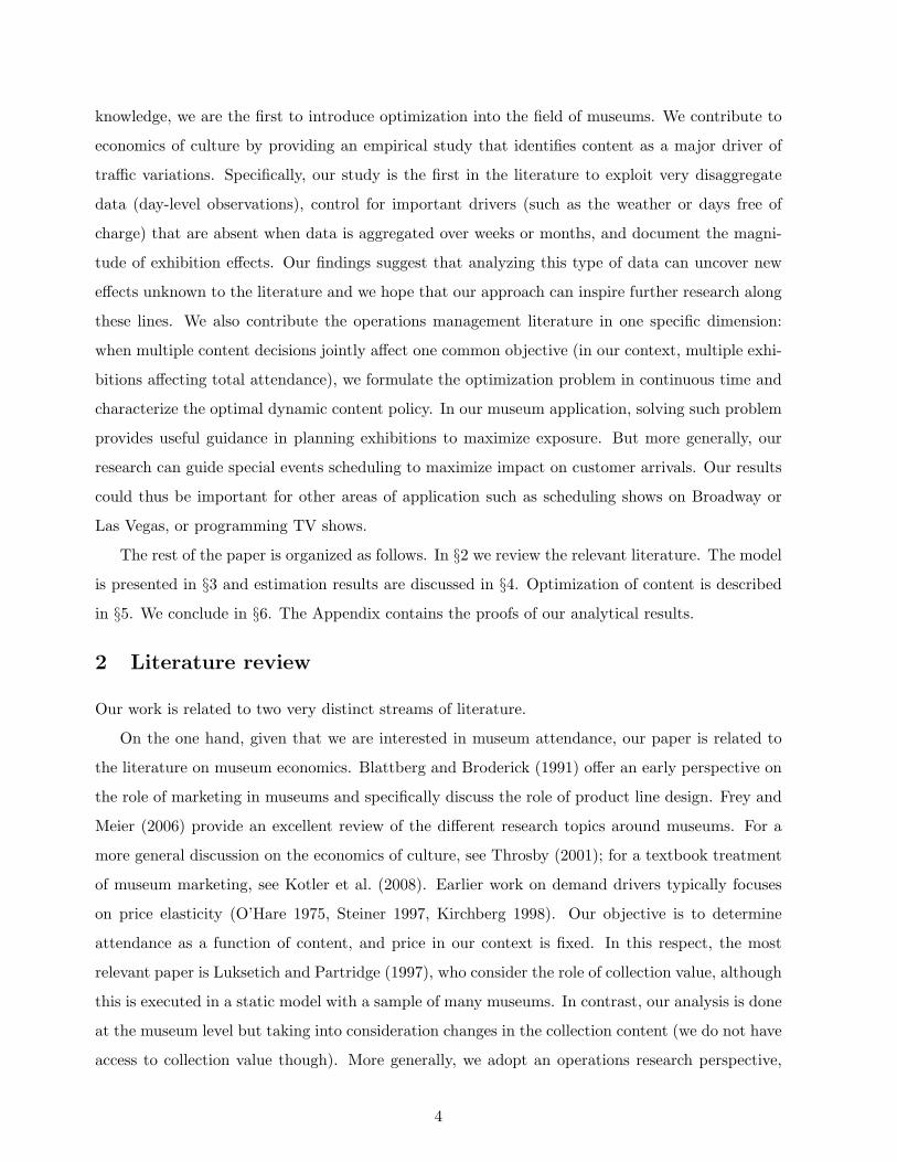
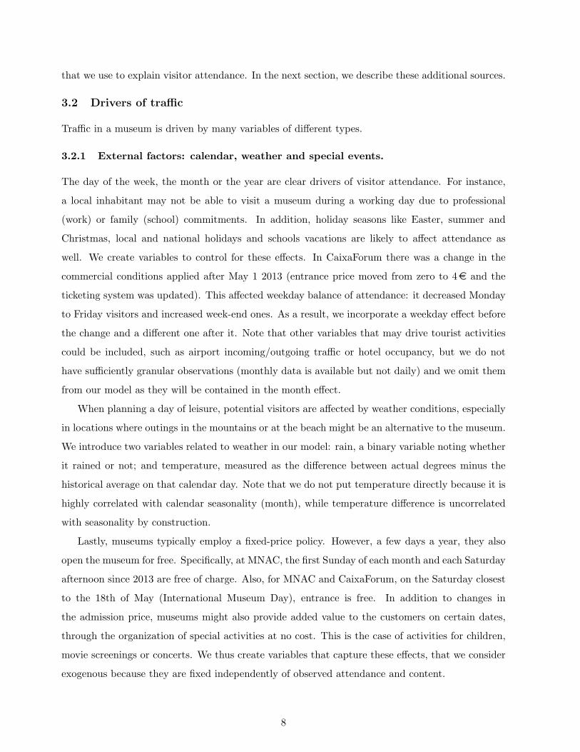
Figure 2: Daily evolution of attendance at MNAC before, during and after the display of theexhibition on Sorolla, the best attended in the history of the museum. Real attendance (solid line)is compared with historical attendance (dashed line) controlling for seasonality.
3.2.2 Internal factors: content.
On top of the previous exogenous factors, there are drivers controllable by museum management.
These are mainly the presence or absence of a temporary exhibition on a certain date. Content
novelty has indeed been identified in the past as a contributor to traffic (Johnson and Thomas
1998). Figure 2 displays the variation of attendance around one particular exhibition at MNAC:
we see that the steep increase in attendance occurs exactly at the times of the exhibition, which
suggests that indeed the exhibition is driving the increase in museum popularity.
To incorporate such drivers, we add a fixed effect for all the days in which the exhibition was
present. Note that this approach usually generates a high number of variables, makes exhibitions
unique and thus makes optimization challenging. For these reasons, we further introduce a structure
to the fixed effect, and make it depend directly on attributes of the exhibition. Namely, the fixed
effect for an exhibition depends on its location (room in which the exhibition was displayed) and
its category, e.g., painting, architecture, etc. Furthermore, in order to take into account temporal
dynamics for every exhibition, we incorporate the effect of exhibition novelty (days since it started)
and remaining availability (days until it was removed). This effect is assumed to be common across
exhibitions. For robustness, we explored alternative specifications as well. Finally, CaixaForum,
months before launching an exhibition, made a forecast of number of visitors/day. This information
can be used as a proxy for the expected quality of the exhibition, although it was dropped in our
models because it turned out to have no significance.
It is worth noting that we had access to social networks (Twitter and Facebook activity) and
9

webpage traffic data. It turned out that this data was highly collinear with exhibition presence.
Thus, incorporating these variables resulted in very small increases of goodness-of-fit and reduced
the significance of all the coefficients. This implies that social media and web information can be
subsumed into our variables for exhibitions and thus can be omitted in the analysis.
In our empirical estimations, exhibitions effects can be interpreted as exogenous. There are
two main reasons for this. First, the choice of exhibition is typically made by curators that do
not work together with museum operations, those that manage the commercial exploitation of the
museum. Curators typically produce exhibitions based on artistic criteria. In particular, they focus
on borrowing pieces of art from other museums and thus are driven by strong supply constraints
that make a ‘commercial’ approach to exhibition design difficult. Second, exhibitions are usually
prepared with a very long lead-time, of the order of 2-3 years. This is due to the coordination that
needs to be put in place to borrow pieces of art from other centers, and sometimes to the fact that
exhibitions may be co-designed with these other museums, so the time in which the exhibition is
shown falls within a long sequence of stops that it makes during its life cycle (e.g., at CaixaForum
Barcelona, exhibitions may travel within the CaixaForum network). To further provide evidence of
this long lead time, the last planning document with all decisions on content, duration and budgets
is issued on average 278 days (minimum in the sample of 20 days) before the exhibition opening.
This implies that the museum management does not cater the design of the exhibition to recent
observations of attendance.
3.3 The model
We propose a multiplicative model for the number of visits at MNAC and CaixaForum, where we
incorporate the elements discussed in §3.2. Formally, our specification is:
log(V isitorst) = α′Xt +∑e∈E
(β0 + β′Yet
)EXHIBet + εt. (1)
In this general formulation, Xt incorporates seasonality and other external factors. EXHIBet
is a binary variable indicating whether exhibition e was running on date t, and Yet incorporates
exhibition features. Hence, our model on the one hand controls for external drivers of attendance,
and on the other proposes a general time-varying structure to capture the impact of content, which
is additive in the features of content.
Xt includes the following variables. We include a time trend t. Ddwt and Mmt are indicator
variables for the event that day t is in weekday d = 1 (Monday) to 7 (Sunday) in window w = 1
10

(before May 1 2013 at CaixaForum) or w = 2 (after), in month m = 1 (January) to 12 (December)
respectively. Hht is an indicator variable for the event that day t is a holiday h, where h ∈ H is
a holiday in Barcelona. RAINt is an indicator variable for the event that day t recorded positive
rain in Barcelona. ∆TEMPt is the difference between average daily temperature and the past
historical average on the same day. FREEft is an indicator variable for the event that day t is
a day free of charge and f ∈ {Saturday, Sunday, Int′l Museum Day,Only Locals}. Aat is an
indicator variable for the event that the activity a is carried out on day t.
In the main model, Yet is a vector that includes the following sets of variables. First, we include a
fixed effect for the 8 types of possible content (Architecture, Cinema, Modern, Photography, History,
Humanitarian, Painting or Other), i.e., binary variables such as Architectureet = 0 or 1. In other
words, the overall effect of a given category, e.g., painting, appears as βPaintingPaintingt where
Paintingt =∑
e PaintingetEXHIBet, and similarly with the rest of the categories. Second, we
also include a fixed effect for the 5 possible physical spaces where e was held (rooms 1 or 2 at MNAC,
rooms 1 to 5 at CaixaForum), i.e., binary variables such as Room1et = 0 or 1 (corresponding to the
fixed effect for room 1). Because for each exhibition the sum of each of these categorical variables is
always one, to avoid overspecifying the model we set the coefficient for Architectureet and Room1et
to be zero. Third, besides these time-invariant variables, we include two time-dependent variables,
namely AGEet = t− Starte (where Starte is the day before the start of the exhibition, so AGEet
takes integer values above 1); and REMAININGet = Ende − t (where Ende is the day after the
end of the exhibition). We include these variables in their log form. The chosen specification varies
steeply when AGEet or REMAININGet are close to one, and are quite flat otherwise. These two
covariates are intended to capture how attendance is affected by beginning and ending of exhibition
effects on potential visitors. Indeed, one would expect attendance to be high when an exhibition
opens, because of the value of novelty; similarly, a few days before the closing, potential visitors
may feel the pressure of the “last call” and attendance should consequently increase.
Note that alternative specifications are described later in §4.3, which include individual fixed
effects for each exhibition, exhibition-dependent life-cycles and other nonlinear forms for beginning
and end of exhibition effects.
We compare four models with variations of the structure in Equation (1). Model (0) includes
only calendar and weather effects in α′Xt, independent of events at the museums, while (1) also
adds the effect of free entrance and museum activities. Model (2) adds the fixed effect of exhibition
attributes (in which Yet is time-invariant), while (3) further includes the effect of exhibition lifecycle
in Yet.
11

We estimate Equation (1) by Generalized Least Squares (GLS). To avoid possible heteroscedas-
ticity issues, we use robust errors and report significance using robust p-values in our results.
4 Empirical Results
We first present the estimation of our model for the entire data in §4.1, validate the results in §4.2
and finally study robustness issues in §4.3.
4.1 Estimates
We estimated the parameters in (1) for several variations, as discussed in the previous section. The
results are shown in Table 2 and 3.
Model (0) (1) (2) (3)
Calendar fixed effects Yes Yes Yes YesFree entrance and activities No Yes Yes Yes
Trend (days) 0.00005*** -0.00006*** -0.00004*** -0.00005***Rain -0.001 0.009 0.012 0.009
Temperature vs. historical -0.002 -0.002 -0.001 -0.001
Number of exhibitions 0.014 0.07Other 0.238*** 0.246***
Cinema 0.005 0.01Contemporary 0.037*** 0.042***Photography 0.008 0.028*
History 0.074*** 0.064***Humanitarian -0.05 0.045
Painting 0.161*** 0.158***Room2 -0.095* 0.009Room3 0.037 0.123**Room4 0.081 0.177***Room5 0.041 0.125**
Log(Age) -0.024***Log(Remaining) -0.018***
R2 38.4% 48.7% 56.8% 57.2%Residual error 0.325 0.298 0.274 0.273
Degrees of freedom 2454 2429 2417 2415F-statistic 26.795 28.077 33.744 33.628
Table 2: Regression results for CaixaForum center. Significance levels: *** (<1%), ** (<5%), *(<10%).
Let us highlight the main insights from the results. First of all, model (0) only captures
external effects, including day of week and month seasonality, weather and holidays. These are
independent of the museum yet explain 38% and 27% of variation for CaixaForum and MNAC
respectively. This implies that seasonality is strong, which is reasonable for two main reasons:
12

Model (0) (1) (2) (3)
Calendar fixed effects Yes Yes Yes YesFree entrance and activities No Yes Yes Yes
Trend (days) 0.00019*** 0.00016*** 0.00020*** 0.00021***Rain 0.044 ** 0.045 *** 0.033 ** 0.040 **
Temperature vs. historical -0.012*** -0.011*** -0.009*** -0.009***
Number of exhibitions 0.002 0.049*Contemporary 0.140*** 0.253***Photography 0.202*** 0.328***
History 0.095** 0.182***Painting 0.265*** 0.373***Room2 -0.115*** -0.104***
Log(Age) -0.008Log(Remaining) -0.038***
R2 27.4% 48.4% 53.7% 54.1%Residual error 0.459 0.387 0.368 0.366
Degrees of freedom 2666 2662 2656 2654F-statistic 20.577 47.098 52.107 51.262
Table 3: Regression results for MNAC. Significance levels: *** (<1%), ** (<5%), * (<10%).
museum visits tend to be holiday and week-end activities, and touristic flows fluctuate over the
year in a predictable fashion. The weather also has an impact on attendance, especially at MNAC:
rain increases attendance by about 4.4%, while higher temperatures reduce attendance by 1.2% per
degree. This means that the museum is more competitive against alternatives on rainy or colder
days, which could be outdoor entertainment or even work (Connolly 2008). In contrast, weather
is not statistically significant for CaixaForum possibly because this museum is better connected to
the city, public transportation and parking garages, so it should be less affected by the weather.
Model (1) increases R2 significantly to 49% and 48% respectively. This increase is mostly due to
the effect of activities at CaixaForum on the one hand (of which evening events and activities for
children have the most impact), and the effect of free entrance at MNAC, once a month at least.
These two models are really capturing effects independent of museum content. Models (2) and (3)
introduce the effect of exhibitions, with static (model 2) or dynamic effects (model 3).
We can see that by adding a few static variables associated with exhibitions, we are able to
improve R2 significantly from model (1) to model (2), to 57% and 54% respectively. This suggests
that indeed there is a strong statistical association between museum content and attendance. Our
specification seems to capture a high portion of residual uncertainty, compared to model (1), with a
limited amount of explanatory variables. Interestingly, while more exhibitions do not significantly
increase attendance (β0 is estimated at 0.014 in CaixaForum and at 0.002 at MNAC - both not
significant), the type of exhibition does have a strong impact on attendance: Painting seems to
13

−0.15
−0.10
−0.05
0 25 50 75Day of exhibition
Figure 3: Impact of lifecycle for an exhibition lasting 90 days at MNAC, as calculated from model(3): −0.008 log(AGEet)− 0.038 log(REMAININGet).
have the most positive effect in both museums. Specifically, the impact of one additional Painting
exhibition is an expected increase in attendance of 0.161 at CaixaForum and 0.265 at MNAC,
in comparison with one additional exhibition on Architecture (the benchmark in the categorical
variables used). Exhibitions on mixed themes (Other), Contemporary, History or Photography also
increase attendance. Furthermore, the location of the exhibition is important too. At CaixaForum,
an additional exhibition in rooms 3, 4 and 5 brings more visitors, in comparison with one in room 1
(benchmark). This is intuitive because these areas usually host the largest exhibitions. In contrast,
room 2 makes less impact than room 1. These areas host smaller exhibitions with more social and
avantgarde topics. The same happens at MNAC, where room 2 is less impactful than room 1,
because it is smaller in size.
Finally, model (3) adds dynamic effects related to the lifecycle of each exhibition. We see that
there are significant beginning- and end-of-exhibition increases in attendance. Figure 3 displays
the predicted impact of exhibition age on attendance, for an exhibition lasting 90 days at MNAC.
We see from this example that the lowest attendance is reached on day 15. It is 1.0% lower than
on the day of exhibition opening, and 15.1% lower than on the day of closing. Interestingly, at
MNAC, the effects at the end of an exhibition are stronger than at the beginning, while they are
balanced at CaixaForum.
It is worth highlighting a potential complication around the estimation of exhibition dynamics.
Specifically, since we also include a linear trend and month dummies, it is possible that exhibition
dynamics are confounded by these other controls. This is the reason why we cannot include the
linear covariate AGEet directly, because it is collinear with the linear time trend and cannot be
identified. We report in §4.3 alternative specifications that suggest that indeed beginning- and
end-of-exhibition effects are strong, regardless of the model used.
14

Training set Validation setTraining set until Validation until MPE MAPE MPE MAPE
CaixaForum June 30, 2013 December 31, 2013 0% 21% -20% 27%December 31, 2013 June 30, 2014 0% 21% 10% 24%
June 30, 2014 December 31, 2014 0% 21% 6% 23%
MNAC June 30, 2013 December 31, 2013 1% 29% 41% 50%December 31, 2013 June 30, 2014 1% 30% -26% 29%
June 30, 2014 December 31, 2014 1% 30% 44% 50%
Table 4: Validation of model (3).
4.2 Out-of-Sample Validation
After showing our model results, we test their out-of-sample forecast accuracy. For this purpose, we
evaluate the quality of model (3) splitting data into two sets, the estimation and the validation set.
The estimation set is used to calibrate model parameters and then these parameters are used in the
validation set to create a forecast of visitors, V isitorst, that is compared to the actual visitor figure.
We run this analysis for three different time windows: training sets until Jun 2013, Dec 2013 and
Jun 2014, and validation sets Jul-Dec 2013, Jan-Jun 2014 and Jul-Dec 2014 respectively. We report
the mean percentage errors (MPE), defined as the expectation of V isitorst/ V isitorst − 1, and the
mean absolute percentage error (MAPE), expectation of∣∣∣V isitorst/ V isitorst − 1
∣∣∣, in Table 4.
There are two key insights that we obtain from Table 4. First, we see that in the training
sets the average error MPE is almost zero, while in the validation sets it fluctuates, especially at
MNAC (deviations up to 44%), although they are also high at CaixaForum (-21%). This means
that a six-month time window is sufficiently long to be subject to the effect of new exhibitions that
may change the six-month average significantly. The same is true for longer validation windows,
which suggests that exhibition heterogeneity cannot be captured easily. Indeed, models that only
take attributes into account, as model (3), will remain inaccurate, while models that take into
account specific exhibition presence, as model (5), will result in overfitting and thus are not useful
for forecasting.
Second, we see that when the average error is small, the average absolute error MAPE in the
validation set is similar to that of the training set, which means that prediction behaves similar to
errors in the training set. However, when the MPE deviation is large, the MAPE becomes much
larger in the validation set compared to the training set. This is because the average is very different
so the absolute deviation is the sum of the MPE plus an error, which is on average approximately
the MPE. This suggests that, when there is no significant difference in the MPE (i.e., no strong
shocks from exhibitions), our model does not seem to overfit the data and hence can be a useful
15

−50
0
50
Jan Feb Mar Apr May Jun JulDate
% e
rror
of f
orec
ast
−50
0
50
100
150
Jul Aug Sep Oct Nov Dec JanDate
% e
rror
of f
orec
ast
Figure 4: Percentage error V isitorst/ V isitorst − 1 of the model at CaixaForum for the validationperiods Jan-Jun and Jul-Dec 2014.
tool for forecasting attendance.
To provide further details on this out-of-sample validation, we plot in Figure 4 the daily errors
in two of the validation periods where MPE remains small. We see that the errors between forecast
and reality are reasonably well spread around zero, with concentrations away from zero in particular
periods, e.g., January, June or September.
4.3 Robustness
In this section, we verify the robustness of the conclusions from §4.1. In particular, we are
interested in exploring the heterogeneity across exhibitions, which we analyze through individual
fixed effects; in allowing other nonlinear forms of beginning- and end-of exhibition effects, which
we analyze with dummies for weeks after opening and before closing; in allowing different life-
cycle patterns across exhibitions, which we analyze through interactions of the dynamic variables,
log(AGEet) and log(REMAININGet), with exhibition features; and in assessing possible satiation
or complementarity effects when several exhibitions of the same type are displayed, which we analyze
with a non-additive model.
16
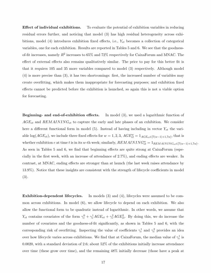
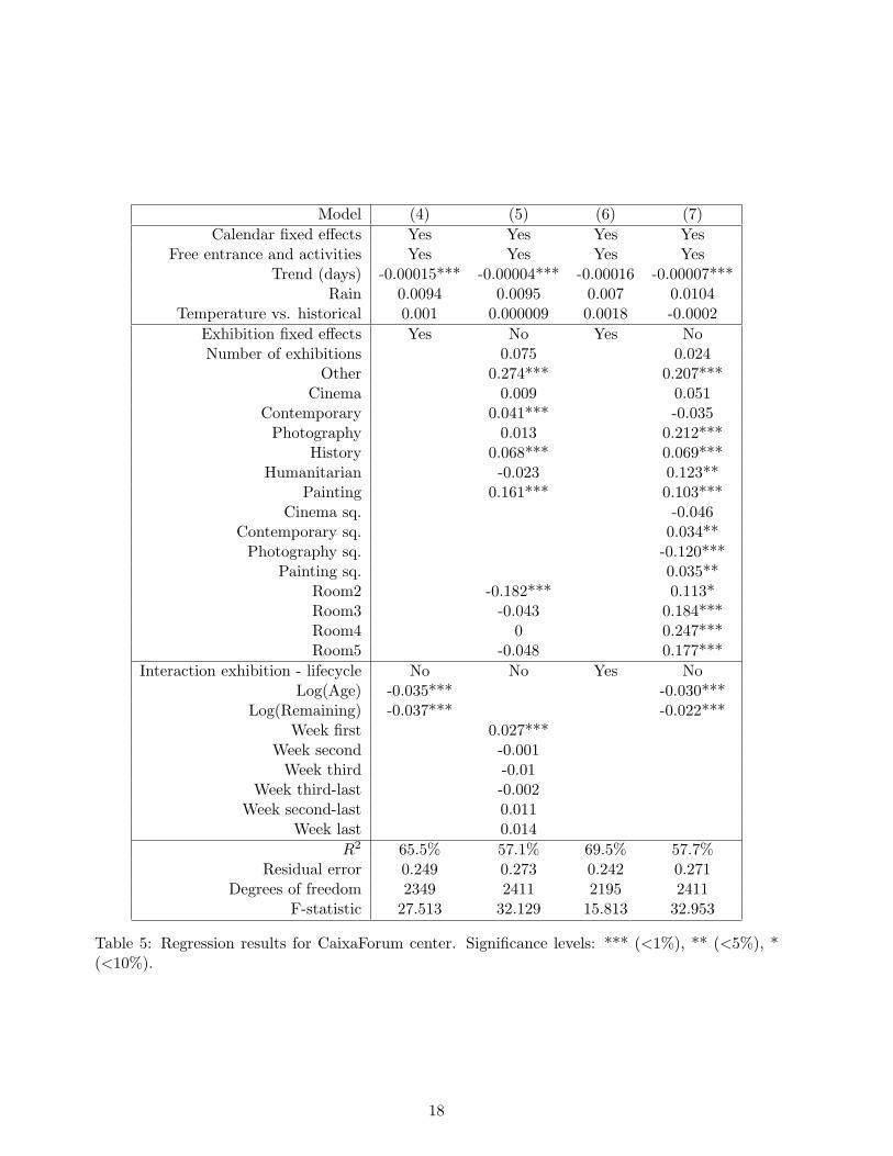
Effect of individual exhibitions. To evaluate the potential of exhibition variables in reducing
residual errors further, and noticing that model (3) has high residual heterogeneity across exhi-
bitions, model (4) introduces exhibition fixed effects, i.e., Yet becomes a collection of categorical
variables, one for each exhibition. Results are reported in Tables 5 and 6. We see that the goodness-
of-fit increases, namely R2 increases to 65% and 72% respectively for CaixaForum and MNAC. The
effect of external effects also remains qualitatively similar. The price to pay for this better fit is
that it requires 105 and 35 more variables compared to model (3) respectively. Although model
(4) is more precise than (3), it has two shortcomings: first, the increased number of variables may
create overfitting, which makes them inappropriate for forecasting purposes; and exhibition fixed
effects cannot be predicted before the exhibition is launched, so again this is not a viable option
for forecasting.
Beginning- and end-of-exhibition effects. In model (3), we used a logarithmic function of
AGEet and REMAININGet to capture the early and late phases of an exhibition. We consider
here a different functional form in model (5). Instead of having including in vector Yet the vari-
able log(AGEet), we include three fixed effects for w = 1, 2, 3, AGEwet = 1AGEet∈[7(w−1)+1,7w], that is
whether exhibition e at time t is in its w-th week; similarly, REMAININGwet = 1REMAININGet∈[7(w−1)+1,7w].
As seen in Tables 5 and 6, we find that beginning effects are quite strong at CaixaForum (espe-
cially in the first week, with an increase of attendance of 2.7%), and ending effects are weaker. In
contrast, at MNAC, ending effects are stronger than at launch (the last week raises attendance by
13.9%). Notice that these insights are consistent with the strength of lifecycle coefficients in model
(3).
Exhibition-dependent lifecycles. In models (3) and (4), lifecycles were assumed to be com-
mon across exhibitions. In model (6), we allow lifecycle to depend on each exhibition. We also
allow the functional form to be quadratic instead of logarithmic. In other words, we assume that
Yet contains covariates of the form γ0e + γ1eAGEet + γ2eAGE2et. By doing this, we do increase the
number of covariates and the goodness-of-fit significantly, as shown in Tables 5 and 6, with the
corresponding risk of overfitting. Inspecting the value of coefficients γ1e and γ2e provides an idea
over how lifecycle varies across exhibitions. We find that at CaixaForum, the median value of γ1e is
0.0020, with a standard deviation of 2.6; about 52% of the exhibitions initially increase attendance
over time (these grow over time), and the remaining 48% initially decrease (those have a peak at
17
Model (4) (5) (6) (7)
Calendar fixed effects Yes Yes Yes YesFree entrance and activities Yes Yes Yes Yes
Trend (days) -0.00015*** -0.00004*** -0.00016 -0.00007***Rain 0.0094 0.0095 0.007 0.0104
Temperature vs. historical 0.001 0.000009 0.0018 -0.0002
Exhibition fixed effects Yes No Yes NoNumber of exhibitions 0.075 0.024
Other 0.274*** 0.207***Cinema 0.009 0.051
Contemporary 0.041*** -0.035Photography 0.013 0.212***
History 0.068*** 0.069***Humanitarian -0.023 0.123**
Painting 0.161*** 0.103***Cinema sq. -0.046
Contemporary sq. 0.034**Photography sq. -0.120***
Painting sq. 0.035**Room2 -0.182*** 0.113*Room3 -0.043 0.184***Room4 0 0.247***Room5 -0.048 0.177***
Interaction exhibition - lifecycle No No Yes NoLog(Age) -0.035*** -0.030***
Log(Remaining) -0.037*** -0.022***Week first 0.027***
Week second -0.001Week third -0.01
Week third-last -0.002Week second-last 0.011
Week last 0.014
R2 65.5% 57.1% 69.5% 57.7%Residual error 0.249 0.273 0.242 0.271
Degrees of freedom 2349 2411 2195 2411F-statistic 27.513 32.129 15.813 32.953
Table 5: Regression results for CaixaForum center. Significance levels: *** (<1%), ** (<5%), *(<10%).
18

Model (4) (5) (6) (7)
Calendar fixed effects Yes Yes Yes YesFree entrance and activities Yes Yes Yes Yes
Trend (days) 0.00029*** 0.00019*** 0.00028*** 0.00021***Rain 0.035 *** 0.036 ** 0.034 *** 0.038 **
Temperature vs. historical -0.009*** -0.007** -0.009*** -0.008**
Exhibition fixed effects Yes No Yes NoNumber of exhibitions 0.03 -0.01
Contemporary 0.229*** 0.200***Photography 0.182*** 0.332***
History 0.076* 0.271***Painting 0.273*** 0.670***
Painting sq. -0.176***Room2 -0.278*** -0.017
Interaction exhibition - lifecycle No No Yes NoLog(Age) -0.019 -0.006
Log(Remaining) -0.037*** -0.034***Week first 0.04
Week second 0.068**Week third 0.046*
Week third-last 0.002Week second-last 0.058**
Week last 0.139***
R2 72.4% 55.8% 74.5% 55.3%Residual error 0.285 0.359 0.277 0.361
Degrees of freedom 2631 2650 2575 2653F-statistic 82.291 51.561 53.64 52.925
Table 6: Regression results for MNAC. Significance levels: *** (<1%), ** (<5%), * (<10%).
19
launch and then there is less interest). Similarly, the median value of γ2e at CaixaForum is 0.000002
with a standard deviation of 0.013; 50% of exhibitions have a positive value of γ2e , resulting in
a positive end-of-exhibition effect. This suggests that there is a high degree of heterogeneity in
lifecycle patterns. At MNAC, such variation across exhibitions is less: the median value of γ1e is
-0.0029, its standard deviation 0.25, about 45% of the exhibitions initially increase attendance over
time (these grow over time), and the other 55% initially decrease (those have a peak at launch and
then there is less interest); the median value of γ2e is 0.00003 with a standard deviation of 0.004,
65% of exhibitions have a positive value of γ2e , resulting in a positive end-of-exhibition effect. At
MNAC, these stronger ending effects are consistent with models (3) and (5).
Theme variety vs. complementarity. The base model (3) assumed that the effect of exhibi-
tions was additive, in the sense that we could use covariates such as Paintingt =∑
e PaintingetEXHIBet.
This implies that having two painting exhibitions simultaneously doubles the average effect on at-
tendance. In reality, these two exhibitions could reinforce each other, attracting even more visitors.
In this case, there would be complementarity across exhibitions. Alternatively, it could be that
customers became satiated with too much painting, making the marginal effect of the second ex-
hibition less than that of the first. In the latter case, exhibitions would be substitutes. To test
such effects, we formulate model (7) where the different thematic variables (Paintingt,Historyt,
etc.) are included in its linear and quadratic form. At MNAC, where only two rooms are available,
the only category which had two simultaneous exhibitions was Painting; at the larger CaixaForum,
there were occasions with at least two Cinema, Contemporary, Painting and Photography exhibi-
tions. The results in Tables 5 and 6 show that the sign of the theme-squared coefficients may be
moderately positive (e.g., Contemporary2t or Painting2t at CaixaForum) or quite negative (e.g.,
Photography2t at CaixaForum or Painting2t at MNAC). Despite the inconclusive results, it is worth
highlighting that our model is able to detect such effects. Future research could further include
cross-sensitivity effects, such as the combinatorial value of themes, e.g., Painting and Architecture
are complements while Painting and History are substitutes.
5 Impact on Museum Operations
Once we have gained an understanding on how content impacts visitor attendance, we are interested
in determining how to design and schedule exhibitions, which is of interest for a museum sales or
operations manager. Specifically, we define a museum policy as an assignment of exhibition e to a
20

given room in a time window [xe, xe + de], where xe denotes the exhibition’s opening date and de
its duration. Opening a new exhibition e2 after another exhibition e1 takes a set-up time ∆e1,e2 ,
so that xe2 = xe1 + de1 + ∆e1e2 . We focus on the tactical problem where we take the sequence
and locations of exhibitions as fixed, so that we only suggest adjustments to the starting times
and durations of the exhibitions, without altering the set-up times. Because of the coupling before
the finishing and starting times across exhibitions, it is sufficient to modify the starting time of
exhibitions. Specifically, we concentrate on optimizing these decisions over a fixed time window,
in which the starting date of the first exhibition and the finishing date of the last exhibition are
fixed; our decision variables are thus the starting dates of all the exhibitions from the second until
the last one.
Given these possible minor adjustments to the museum plan, there are several objectives that
the museum could pursue. On the one hand, the total number of visitors is important, especially
for private museums: this creates an incentive to develop ‘blockbuster’ exhibitions (Frey and Meier
2006), or more generally, to offer in certain moments very attractive content, even if this is for a
short period of time. On the other hand, the well-being of visitors and the quality of the visitor’s
experience are also important. This means that congestion may have a negative effect, thereby
pushing museums to spread visits over time as opposed to concentrating them in some days or
months. Finally, there may be costs associated with extending the duration of certain exhibitions,
or additional revenues from promotional activities.
To jointly deal with these objectives, we introduce a utility function u(vt) derived from attracting
an expected number of visitors vt on a particular day t. If the only objective is to maximize profit
(with entrance fee is p) then u(vt) = pvt. If on the other hand we do not value attendance beyond a
given threshold v, then we can let u(vt) = pmin{v, vt}. We assume that u is an increasing concave
function, so that the marginal value of additional attendance is high when the museum’s current
load is light, and low when it is heavily loaded. Furthermore, to account for possible costs and
additional revenues from the presence of an exhibition, we can also include a variable cost ce related
to carrying exhibition e in every period.
Given that there are several rooms in the museum, and denoting yet = 1xe≤t≤xe+de the binary
variable for exhibition e being active in period t, the total utility for the museum is equal to
U :=
T∑t=0
δt
[u(eαt+
∑e yetβe(t,xe,de)
)−∑e
ceyet
](2)
where αt, βe(·) are time and exhibition factors that can be obtained from one of our forecast models
in (1) and δ is a discount factor.
21
For tractability, given that days are relatively short compared to the duration of exhibitions and
to obtain stronger analytical results, we employ a continuous formulation instead of the discrete one
(so we can take derivatives rather than differences). We further make four simplifying assumptions
although similar results can be obtained in general. First, we use the logarithmic specification of
model (3): γe(t, xe, de) = −λ ln(t − xe + 1) − µ ln(xe + de − t + 1) where λ, µ > 0. Second, we
concentrate on the case u(vt) = min{vθt , v
}with θ ∈ [0, 1] is a parameter that affects concavity
and v that penalizes for high attendance figures; they both capture the aversion for variability in
attendance over time. Third, we take set-up times to be constant, i.e., ∆e1,e2 = ∆ for all e1, e2.
Fourth, we assume that ce are identical across exhibitions, so that∑T
t=0
∑e ceyet is independent of
xe; this allows us to ignore costs in the analysis, so we can set ce = 0 in what follows.
In this setting, the objective becomes
U :=
∫ T
t=0min
eαt
∏e|yet=1
eβe
(t− xe)λ(xe + de − t)µ
, v
dt (3)
where αt = θαt − ln(δ)t, βe = θβe, λ = θλ and µ = θµ. Since 0 ≤ λ, µ, λ+ µ < 1 (given the values
observed in our empirical study), the integrals converge and are thus well-defined.
We can now maximize U by adjusting the duration of exhibitions. Note that our model is flexible
and optimization could also change exhibition characteristics (type, room where it is located), but
this would require a change in the artistic contents. In particular, it may have a long-lasting impact
on attendance that is not captured by our regression model, so it is beyond the scope of this paper.
Tackling this effect would require models that incorporate visitor experience factors (Dixon and
Verma 2013, Das Gupta et al. 2015, Tereyagoglu et al. 2017, 2015) or market size dynamics (Caro
and Martınez-de-Albeniz 2017).
We next formulate and describe optimal policies for a museum with two different perspectives.
First, we analytically characterize the optimal duration of exhibitions when the museum runs a
single exhibition at a time. Second, we optimally coordinate the schedules of several exhibitions
running in parallel and determine the impact of concentrating all openings at the same time vs.
spreading them. Finally, we jointly optimize both duration and coordination for the 2014 program
at CaixaForum, to see how the two levers interact.
5.1 Optimizing exhibition duration
We analyze here how to maximize U in (3) when there is a single room and exhibitions e = 1, . . . , E
have to be scheduled within a time window [0, T ]. For tractability of the analysis, we assume v = ∞
in this section (in §5.3 we numerically study v ≤ ∞).
22
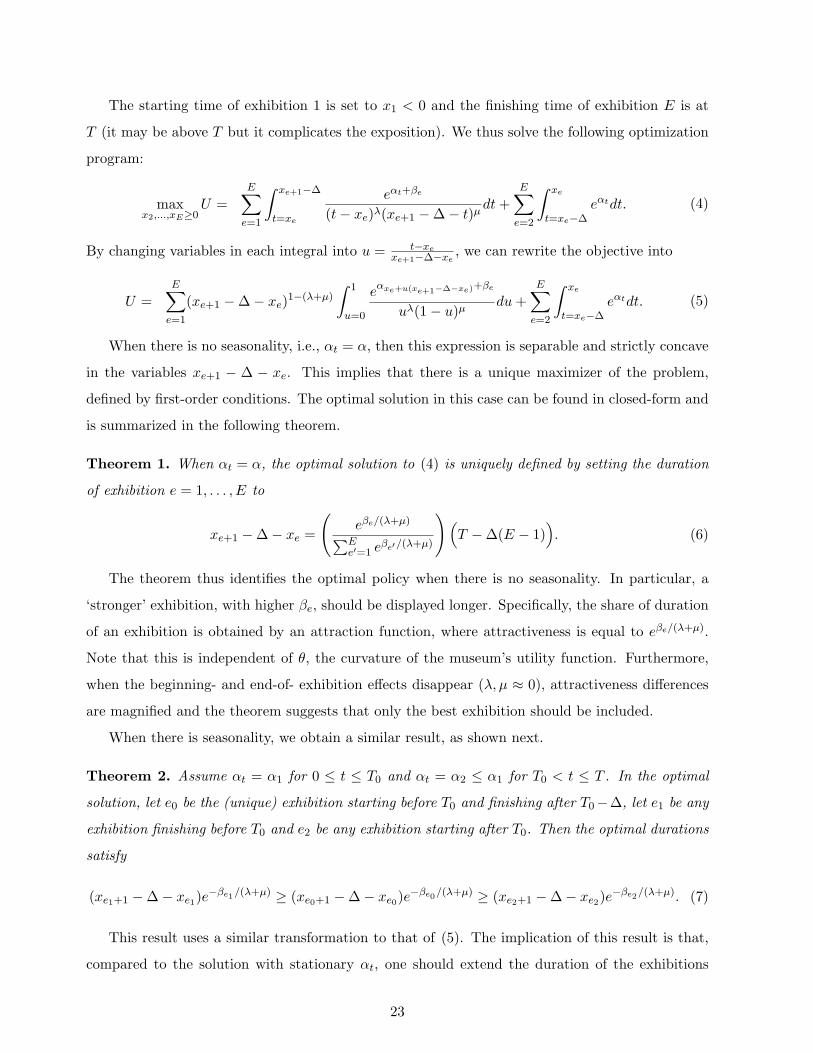
The starting time of exhibition 1 is set to x1 < 0 and the finishing time of exhibition E is at
T (it may be above T but it complicates the exposition). We thus solve the following optimization
program:
maxx2,...,xE≥0
U =
E∑e=1
∫ xe+1−∆
t=xe
eαt+βe
(t− xe)λ(xe+1 −∆− t)µdt+
E∑e=2
∫ xe
t=xe−∆eαtdt. (4)
By changing variables in each integral into u = t−xexe+1−∆−xe
, we can rewrite the objective into
U =E∑
e=1
(xe+1 −∆− xe)1−(λ+µ)
∫ 1
u=0
eαxe+u(xe+1−∆−xe)+βe
uλ(1− u)µdu+
E∑e=2
∫ xe
t=xe−∆eαtdt. (5)
When there is no seasonality, i.e., αt = α, then this expression is separable and strictly concave
in the variables xe+1 − ∆ − xe. This implies that there is a unique maximizer of the problem,
defined by first-order conditions. The optimal solution in this case can be found in closed-form and
is summarized in the following theorem.
Theorem 1. When αt = α, the optimal solution to (4) is uniquely defined by setting the duration
of exhibition e = 1, . . . , E to
xe+1 −∆− xe =
(eβe/(λ+µ)∑E
e′=1 eβe′/(λ+µ)
)(T −∆(E − 1)
). (6)
The theorem thus identifies the optimal policy when there is no seasonality. In particular, a
‘stronger’ exhibition, with higher βe, should be displayed longer. Specifically, the share of duration
of an exhibition is obtained by an attraction function, where attractiveness is equal to eβe/(λ+µ).
Note that this is independent of θ, the curvature of the museum’s utility function. Furthermore,
when the beginning- and end-of- exhibition effects disappear (λ, µ ≈ 0), attractiveness differences
are magnified and the theorem suggests that only the best exhibition should be included.
When there is seasonality, we obtain a similar result, as shown next.
Theorem 2. Assume αt = α1 for 0 ≤ t ≤ T0 and αt = α2 ≤ α1 for T0 < t ≤ T . In the optimal
solution, let e0 be the (unique) exhibition starting before T0 and finishing after T0−∆, let e1 be any
exhibition finishing before T0 and e2 be any exhibition starting after T0. Then the optimal durations
satisfy
(xe1+1 −∆− xe1)e−βe1/(λ+µ) ≥ (xe0+1 −∆− xe0)e
−βe0/(λ+µ) ≥ (xe2+1 −∆− xe2)e−βe2/(λ+µ). (7)
This result uses a similar transformation to that of (5). The implication of this result is that,
compared to the solution with stationary αt, one should extend the duration of the exhibitions
23

0 0.05 0.1 0.15 0.2 0.25 0.3
Seasonality variation χ
100
200
300
Opt
imal
sta
rt/e
nd ti
mes
Exhib. 3 start Exhib. 2 end Exhib. 2 start Exhib. 1 end
0 50 100 150 200 250 300 350
Time t
0
1
2
3
Exp
ecte
d at
tend
ance
χ=0.3
Figure 5: On the left, optimal starting times for different seasonality patterns αt = −χ(2t/T − 1)(average zero and decreasing from χ to −χ), as a function of χ. On the right, expected attendanceover time, for χ = 0.3. The parameters used are E = 3, λ = µ = 0.02, βe = 0.5 for all e, ∆ = 30days and T = 360 days.
during the period with higher αt (any e1 as stated in the theorem) and reduce it during the rest of
the horizon (e0 or any e2). This implies that, when there are two exhibitions with the same impact
(same βe), the one displayed in periods with higher traffic (higher αt) should be displayed longer.
Figure 5 illustrates this insight using a decreasing seasonality pattern αt = 1−χ(2t/T−1), where
χ ≥ 0 is a parameter to control for variation between the beginning and the end of the horizon,
i.e., α0 = χ and αT = −χ. We see that indeed, as more variation occurs during the horizon, at
optimality early exhibitions are programmed during a longer duration, while late exhibitions are
shorter. For instance, when there is no seasonality (χ = 0), all three exhibitions last for 100 days;
in contrast, when χ = 0.3, the first exhibition lasts for 117 days, the second for 99 days, and the
third for 84 days. This suggests that the insight from Theorem 2 is valid in more general settings.
5.2 Multiple exhibitions in parallel
The previous section has examined how exhibition duration should be balanced when there is at
most one exhibition running at a time. When there is more than one exhibition area in the museum,
i.e., a number of rooms R ≥ 2, a second decision must be taken: how to coordinate the opening
and closing times of exhibitions, in addition to their durations. In essence this question boils down
to deciding whether the museum wants to synchronize exhibitions, so they all start together, which
results in peak periods during beginning and end exhibition times; or to stagger them over time so
in any period there is one exhibition opening or finishing, which results in more stable attendance
patterns. Different museums may have different policies regarding this decision. For example,
at CaixaForum, opening times were almost always staggered to avoid concentrations of activity
around the same date; but there were occasions where exhibitions closed on the same exact day,
24
e.g., Sorolla y el mar and Reduccions Jesuites closed on Sep. 14, 2014.
We study those in this section, under tractable assumptions (we numerically optimize this
problem without assumptions in §5.3). To concentrate on the synchronization question, we assume
here that v = ∞, all exhibitions are identical (βe = β), there is no seasonality (αt = α = 0)
and moreover there are Er = E exhibitions planned for each room r = 1, . . . , R. Under these
parameters, Theorem 1 suggested under R = 1 that all exhibitions should be equally long. So we
impose that the duration of all exhibitions is set to D = T/E − ∆ where T is the length of the
planning horizon. As a result of this imposition, and setting without loss of generality x1,1 = 0,
the only decisions that the museum must take are the starting times of xr,1 for r = 2, . . . , R. In
other words, we study the coordination of starting times assuming that visits follow cycles of length
D +∆ = T/E, i.e., attendances at t and t+D +∆ are identical for all t. We can thus set E = 1
without loss of generality, so we can omit the exhibition sub-index e.
The optimization problem can thus be expressed as follows:
maxxr≥0
U =∫ Tt=0
(∏r|xr≤t≤xr+T−∆
eβ
(t−xr)λ(xr+T−∆−t)µ
)(∏r|xr−T≤t≤xr−∆
eβ
(t−xr+T )λ(xr−∆−t)µ
)dt. (8)
Integrals are well-defined provided that λR, µR < 1. Note that, at t, the elements from the first
product come from exhibitions that have started in [0, t], while those from the second product from
exhibitions that started before 0.
Consider the first-order condition with respect to xr, assuming that the other decisions are fixed.
Letting ϕ(t) =(∏
r′ =r|xr′≤t≤xr′+T−∆eβ
(t−xr′ )λ(xr′+T−∆−t)µ
)(∏r′ =r|xr′−T≤t≤xr′−∆
eβ
(t−xr′+T )λ(xr′−∆−t)µ
),
when xr −∆ < 0, U can be rewritten as:
∫ xr
t=0ϕ(t)dt+ eβ(T −∆)1−(λ+µ)
∫ 1
u=0
ϕ(xr + (T −∆)u
)uλ(1− u)µ
du+
∫ T
t=xr+T−∆ϕ(t)dt.
This expression is differentiable at all points where ϕ is continuous. The first-order condition can
thus be expressed as:
ϕ(xr)− ϕ(xr + T −∆) + eβ(T −∆)1−(λ+µ)
∫ 1
u=0
ϕ′(xr + (T −∆)u
)uλ(1− u)µ
du = 0. (9)
Note that at points u such that xr +(T −∆)u = xr′ , xr′ −∆ or xr′ +T −∆, ϕ is discontinuous but
the integral of limϵ→0
∫ u+ϵu=u−ϵ
ϕ′(xr+(T−∆)u
)uλ(1−u)µ
du =limϵ→0
{ϕ
(xr+(T−∆)u+ϵ
)−ϕ
(xr+(T−∆)u−ϵ
)}uλ(1−u)µ
is still
well defined. An equivalent expression to (9) is∫ 1
u=0ϕ′(xr + u(T −∆)
)( eβ
uλ(1− u)µ− 1
(T −∆)λ+µ
)du = 0. (10)
When xr −∆ ≥ 0, U has a different expression but the optimality condition is also (10).
25

1.1 1.15 1.2 1.25 1.3 1.35 1.4
Congestion cap
20
40
60
80
100
120
Opt
imal
sta
rt ti
mes
Exhib. 3 startExhib. 2 start
Figure 6: Optimal starting times as a function of congestion cap v. R = 3, λ = µ = 0.02, eβ = 0.2,∆ = 30 and T = 120.
It turns out that, although the optimality condition is hard to solve, we find that in certain
cases, optimal solutions are always reached at the extreme point xr = 0, as shown next.
Theorem 3. When v = ∞ and eβ(T − ∆)λ+µ(1 + µ
λ
)λ (1 + λ
µ
)µ≥ 1, then is optimal to open
exhibitions at the same time, i.e., xr = 0 for all r = 1, . . . , R.
The technical assumption of the theorem means that it is always better to have an exhibition
present than removing it, even in the lower-attendance, intermediate periods of the exhibition. It is
satisfied for either high β (e.g., positive) or high λ, µ. Under this condition, the theorem establishes
that it is optimal to synchronize starting times. The intuition behind this result is that exhibitions
reinforce each other: this implies that running two exhibitions in parallel increases attendance
at the beginning and end of the exhibition, while it decreases attendance on other intermediate
periods.
This is only true when v = ∞. Indeed, when high attendances are penalized, it is usually best
to stagger them. Figure 6 shows the optimal starting times when v is varied. Recall that as v
decreases, the museum penalizes days with high traffic more. For high v, there are no penalties for
high attendance, so it is best to synchronize all exhibitions (all of them starting around 0, finishing
around T −∆ = 90 and starting again at T = 120), as suggested by Theorem 3. In contrast, for
lower values of v, it is best to avoid very high attendances, and it is optimal to spread exhibitions
evenly over time, and optimal starting times are around 40 and 80.
We thus find that there might be two regimes that a museum should consider. When v is small
enough, i.e., moments of high attendance are discouraged, then it is better to avoid such moments
26

of high traffic. Thus, by staggering exhibition launch times, the highest attendance is reduced,
while the lowest attendance is increased. This seems to be the case at CaixaForum, suggesting
that the museum prioritizes having a steady flow of visitors rather than peaks. In contrast, when
v is larger, it is best to launch all the available exhibitions at the same time. This results in
simultaneous peaks of all the exhibitions, which leads to a few days of extremely high attendance.
These moments push total attendance to the highest possible level. Note that such synchronization
would be further preferred if there are additional complementarity effects such as those identified
in §4.3.
5.3 Counterfactual Scheduling Experiments
After studying the optimization problem along two individual dimensions (durations with one
exhibition at a time and synchronization of multiple exhibitions with fixed duration), we study the
interaction of the two. For this purpose, we numerically reoptimize the 2014 program of rooms
3 and 4 at CaixaForum, using the parameters from our model (3), see Table 2. Specifically, we
consider five exhibitions:
• In room 3, a history exhibition run from 27 Feb. to 15 Jun. (e3 = 1), then a painting one
from 15 Jul. to 5 Jan. of the following year (e3 = 2).
• In room 4, an architecture exhibition run from 29 Jan. to 11 May (e4 = 1), then a painting
one from 12 Jun. to 14 Sep. (e4 = 2), and then a photography one from 15 Oct. until 8 Feb.
of the following year (e4 = 3).
We adjust the opening times of e3 = 2, e4 = 2 and e4 = 3, so that we modify the duration of the
five exhibitions. Note that attendance is here measured over days, as opposed to continuous time
as in §§5.1-5.2. Since we only have data until end of 2014, it only captures the impact on visitors
within the year, i.e., effects on 2015 are not taken into account.
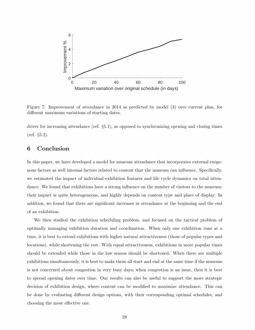
We find that it is best to shorten e3 = 1, e4 = 1 and e4 = 3 as much as possible, while extending
e3 = 2 and e4 = 2 as much as possible. This is because painting exhibitions drive larger audiences
and extending them is better despite weaker mid-exhibition audiences. Figure 7 illustrates the
results, for different variations from the original schedule. Note that for variations of 100 days
over the original schedule, exhibitions others than e3 = 2 and e4 = 2 last for less than one week,
so although the improvement reaches 5.4%, it does imply a major modification of the museum
offering. Less radical interventions yield improvements of lesser magnitude (3.6% for variation of
60 days for instance). We thus see that favoring exhibitions with higher attractiveness is the main
27
0 20 40 60 80 100
Maximum variation over original schedule (in days)
0
2
4
6
Impr
ovem
ent %
Figure 7: Improvement of attendance in 2014 as predicted by model (3) over current plan, fordifferent maximum variations of starting dates.
driver for increasing attendance (ref. §5.1), as opposed to synchronizing opening and closing times
(ref. §5.2).
6 Conclusion
In this paper, we have developed a model for museum attendance that incorporates external exoge-
nous factors as well internal factors related to content that the museum can influence. Specifically,
we estimated the impact of individual exhibition features and life cycle dynamics on total atten-
dance. We found that exhibitions have a strong influence on the number of visitors to the museum:
their impact is quite heterogeneous, and highly depends on content type and place of display. In
addition, we found that there are significant increases in attendance at the beginning and the end
of an exhibition.
We then studied the exhibition scheduling problem, and focused on the tactical problem of
optimally managing exhibition duration and coordination. When only one exhibition runs at a
time, it is best to extend exhibitions with higher natural attractiveness (those of popular types and
locations), while shortening the rest. With equal attractiveness, exhibitions in more popular times
should be extended while those in the low season should be shortened. When there are multiple
exhibitions simultaneously, it is best to make them all start and end at the same time if the museum
is not concerned about congestion in very busy days; when congestion is an issue, then it is best
to spread opening dates over time. Our results can also be useful to support the more strategic
decision of exhibition design, where content can be modified to maximize attendance. This can
be done by evaluating different design options, with their corresponding optimal schedules, and
choosing the most effective one.
28

In summary, this work is the first to apply operations research techniques into the management
of museums. While we have explored levers for operations improvements related to content schedul-
ing, there are many opportunities for further research. First, while the focus of the paper has been
on museums, similar problems occur in other arts settings, such as programming of musicals or
theater plays (The Economist 2016), for which very rich attendance information is available too.
Second, we have considered the optimization of scheduling with a fixed sequence of exhibitions,
that are planned upfront. This is appropriate given the long lead-times to set up an exhibition.
However, when the lead-times are shorter, one could consider closed-loop policies where, in each
period, the museum can decide to continue an exhibition or replace it with something else. Optimal
policies might have very different structure compared to those established in our case, as in Cınar
and Martınez-de-Albeniz (2013). Third, exhibitions involve communication and marketing expenses
along their duration. One can seek how to optimally support exhibitions by optimally balancing
these efforts over time. Fourth, we have seen that there are complementarity and substitution
effects across exhibitions. It would be interesting to further detail the nature of such effects, and in
particular to develop scheduling optimization models that take them into consideration. Finally, in
our research we have used aggregate data of attendance to the museum. When there is individual
information about visits, one can build more powerful attendance models that internalize the effect
of exhibition offer and duration (how new exhibitions are and how much longer they will be shown)
on individual visit decisions. This will require complex behavior models similar to those used in
online retailing (Moe and Fader 2004).
References
Ainslie, A., X. Dreze, and F. Zufryden. 2005. Modeling movie life cycles and market share. MarketingScience 24 (3): 508–517.
Bernstein, F., and V. Martınez-de-Albeniz. 2017. Dynamic Product Rotation in the Presence of StrategicCustomers. Management Science 63 (7): 2092–2107.
Blattberg, R. C., and C. J. Broderick. 1991. Marketing of art museums. In The economics of art museums,327–346. University of Chicago Press.
Caro, F., and V. Martınez-de-Albeniz. 2012. Product and price competition with satiation effects. Manage-ment Science 58 (7): 1357–1373.
Caro, F., and V. Martınez-de Albeniz. 2015. Fast fashion: Business model overview and research opportu-nities. In Retail Supply Chain Management: Quantitative Models and Empirical Studies, 2nd Edition,ed. N. Agrawal and S. A. Smith, 237–264. Springer, New York.
Caro, F., and V. Martınez-de-Albeniz. 2017. Managing Online Content to Build a Follower Base: Model andApplication. Working paper, IESE Business School.
Caro, F., V. Martınez-de Albeniz, and P. Rusmevichientong. 2014. The Assortment Packing Problem:Multiperiod Assortment Planning for Short-Lived Products. Management Science 60 (11): 2701–2721.
Chayka, K. 2010. Are Fine Art Museums the Next Starbucks? The Atlantic April 20:online.
29

Cınar, E., and V. Martınez-de-Albeniz. 2013. A Closed-loop Approach to Dynamic Assortment Planning.Working paper, IESE Business School.
Connolly, M. 2008. Here comes the rain again: Weather and the intertemporal substitution of leisure. Journalof Labor Economics 26 (1): 73–100.
Das Gupta, A., U. S. Karmarkar, and G. Roels. 2015. The design of experiential services with acclimationand memory decay: Optimal sequence and duration. Management Science 62 (5): 1278–1296.
Dixon, M., and R. Verma. 2013. Sequence effects in service bundles: Implications for service design andscheduling. Journal of Operations Management 31 (3): 138–152.
Eliashberg, J., A. Elberse, and M. A. Leenders. 2006. The motion picture industry: Critical issues in practice,current research, and new research directions. Marketing Science 25 (6): 638–661.
Eliashberg, J., Q. Hegie, J. Ho, D. Huisman, S. J. Miller, S. Swami, C. B. Weinberg, and B. Wierenga. 2009.Demand-driven scheduling of movies in a multiplex. International Journal of Research in Marketing 26(2): 75–88.
Eliashberg, J., C. B. Weinberg, and S. K. Hui. 2008. Decision models for the movie industry. In Handbookof marketing decision models, 437–468. Springer.
Fisher, M. 2009. OR FORUM–Rocket Science Retailing: The 2006 Philip McCord Morse Lecture. OperationsResearch 57 (3): 527–540.
Frey, B. S. 1998. Superstar museums: an economic analysis. Journal of Cultural Economics 22 (2-3):113–125.
Frey, B. S., and S. Meier. 2006. The economics of museums. Handbook of the Economics of Art andCulture 1:1017–1047.
Hedrick-Wong, Y., and D. Choong. 2014. 2014 Global Destination Cities Index. Technical report, Master-Card.
Johnson, P., and B. Thomas. 1998. The economics of museums: a research perspective. Journal of CulturalEconomics 22 (2-3): 75–85.
Kirchberg, V. 1998. Entrance fees as a subjective barrier to visiting museums. Journal of Cultural Eco-nomics 22 (1): 1–13.
Kotler, N. G., P. Kotler, and W. I. Kotler. 2008. Museum marketing and strategy: designing missions,building audiences, generating revenue and resources. John Wiley & Sons.
Krider, R. E., and C. B. Weinberg. 1998. Competitive dynamics and the introduction of new products: Themotion picture timing game. Journal of Marketing Research 35:1–15.
Lim, W. S., and C. S. Tang. 2006. Optimal product rollover strategies. European Journal of OperationalResearch 174 (2): 905–922.
Lobel, I., J. Patel, G. Vulcano, and J. Zhang. 2015. Optimizing product launches in the presence of strategicconsumers. Management Science 62 (6): 1778–1799.
Luksetich, W. A., and M. D. Partridge. 1997. Demand functions for museum services. Applied Economics 29(12): 1553–1559.
Martınez-de-Albeniz, V., and A. Saez-de-Tejada. 2014. Dynamic choice models for cultural choice. Workingpaper, IESE Business School.
Moe, W. W., and P. S. Fader. 2004. Capturing evolving visit behavior in clickstream data. Journal ofInteractive Marketing 18 (1): 5–19.
Munoz-Seca, B., and J. Riverola. 2009. Tate: Reinventing Operations for a Different Type of Company.Technical report, IESE Case P-1093-E.
Nasini, S., and V. Martınez-de-Albeniz. 2015. Pairwise influences in dynamic choice: method and application.Working paper, IESE Business School.
O’Hare, M. 1975. Why do people go to museums? The effect of prices and hours on museum utilization1.Museum International 27 (3): 134–146.
Pes, J., and E. Sharpe. 2015. Visitor figures 2014: the world goes dotty over Yayoi Kusama. The ArtNewspaper April 2:online.
30
Popescu, D. G., and P. Crama. 2015. Ad revenue optimization in live broadcasting. Management Science 62(4): 1145–1164.
Radas, S., and S. M. Shugan. 1998. Seasonal marketing and timing new product introductions. Journal ofMarketing Research 35 (3): 296–315.
Steiner, F. 1997. Optimal pricing of museum admission. Journal of cultural economics 21 (4): 307–333.
Swami, S., M. L. Puterman, and C. B. Weinberg. 2001. Play it again, Sam? Optimal replacement policiesfor a motion picture exhibitor. Manufacturing & Service Operations Management 3 (4): 369–386.
Tereyagoglu, N., P. S. Fader, and S. Veeraraghavan. 2015. Pricing Theater Seats: The Value of PriceCommitment and Monotone Discounting. Working paper, The Wharton School.
Tereyagoglu, N., P. S. Fader, and S. Veeraraghavan. 2017. Multiattribute Loss Aversion and ReferenceDependence: Evidence from the Performing Arts Industry. Management Science Forthcoming:NA.
The Economist 2016. How to create a blockbuster musical. The Economist April 25:online.
Throsby, D. 2001. Economics and culture. Cambridge university press.
Turisme de Barcelona 2014. Annual Report.
Van Aalst, I., and I. Boogaarts. 2002. From museum to mass entertainment the evolution of the role ofmuseums in cities. European Urban and Regional Studies 9 (3): 195–209.
Wikipedia 2015. List of most visited art museums in the world. Wikipedia 16 July:online.
WTTC 2016. Travel & Tourism: Economic Impact 2016, Spain. Technical report, World Travel & TourismCouncil.
31

Appendix: Proofs
Proof of Theorem 1
Proof. Setting the derivative of (5) with respect to xe to zero yields
(xe+1 −∆− xe)−(λ+µ)eβe = (xe −∆− xe−1)
−(λ+µ)eβe−1 .
Let this value be equal to A−(λ+µ). This implies that
(xe+1 −∆− xe) = Aeβe/(λ+µ).
Adding this equality across e = 1, . . . , E we obtain T − (E− 1)∆ = A∑E
e′=1 eβe′/(λ+µ), which leads
to (6).
Proof of Theorem 2
Proof. Setting the derivative of (5) with respect to xe such that xe+2 −∆ ≤ T0 or xe−1 ≥ T0 to
zero yields
(xe+1 −∆− xe)−(λ+µ)eβe = (xe −∆− xe−1)
−(λ+µ)eβe−1 .
This is the same condition obtained without seasonality for Theorem 1. Hence for any e1 described
in the theorem we obtain the same value (xe1+1 −∆− xe1)−(λ+µ)eβe1 ; the same is true for any e2.
The difference appears in the first-order condition for xe0 :
(xe1+1 −∆− xe1)−(λ+µ)eβe1
∫ 1
u=0
eα1
uλ(1− u)µdu
= (xe0+1 −∆− xe0)−(λ+µ)eβe0
(∫ au=0
eα1
uλ(1−u)µdu+
∫ 1u=a
eα2
uλ(1−u)µdu− (xe0+1−∆−xe0 )(e
α1−eα2 )
(1−λ−µ)aλ(1−a)µ∂a
∂xe0
)with a =
T0−xe0xe0+1−∆−xe0
; and for xe0+1:
(xe2+1 −∆− xe2)−(λ+µ)eβe2
∫ 1
u=0
eα2
uλ(1− u)µdu
= (xe0+1 −∆− xe0)−(λ+µ)eβe0
(∫ au=0
eα1
uλ(1−u)µdu+
∫ 1u=a
eα2
uλ(1−u)µdu+
(xe0+1−∆−xe0 )(eα1−eα2 )
(1−λ−µ)aλ(1−a)µ∂a
∂xe0+1
).
Since ∂a∂xe0
≥ 0 and ∂a∂xe0+1
≤ 0, and α1 ≥ α2, we have that
(xe1+1 −∆− xe1)−(λ+µ)eβe1 ≤ (xe0+1 −∆− xe0)
−(λ+µ)eβe0
and
(xe2+1 −∆− xe2)−(λ+µ)eβe2 ≥ (xe0+1 −∆− xe0)
−(λ+µ)eβe0 ,
i.e., Equation (7).
32

Proof of Theorem 3
Proof. Given xr′ for r′, let xr be a solution to the first-order condition (10). Noting that
ψ(t) :=ϕ′(t)
ϕ(t)=
∑r′ =r|xr′≤t≤xr′+T−∆
(−λ
t− xr′+
µ
xr′ + T −∆− t
)+
∑r′ =r|xr′−T≤t≤xr′−∆
(−λ
t− xr′ + T+
µ
xr′ −∆− t
)
we have
ψ′(t) =∑
r′ =r|xr′≤t≤xr′+T−∆
(λ
(t− xr′)2+
µ
(xr′ + T −∆− t)2
)+
∑r′ =r|xr′−T≤t≤xr′−∆
(λ
(t− xr′ + T )2+
µ
(xr′ −∆− t)2
)≥ 0.
Letting c = e−β
(T−∆)λ+µ , (10) is equivalent to∫ 1
u=0ψ(xr + u(T −∆)
)ϕ(xr + u(T −∆)
)( 1
uλ(1− u)µ− c
)du = 0.
Note that 1uλ(1−u)µ
is minimized at u = λ/(λ+ µ) and hence
1
uλ(1− u)µ− c ≥ (λ+ µ)λ+µ
λλµµ− c ≥ 0
by assumption. The second derivative of U with respect to xr is thus∫ 1
u=0
(ψ′(xr + u(T −∆)
)+ ψ
(xr + u(T −∆)
)2)ϕ(xr + u(T −∆)
)( 1
uλ(1− u)µ− c
)du > 0.
This implies that any interior solution xr to (10) is a local minimum of U . As a result, the maximum
must be reached at xr = 0 or xr = T (which because of the cyclic nature of the schedule results in
the same plan). The same argument applies to all r.
33