measuring benefits of manpower, personnel… · measuring benefits of manpower, personnel, and...
TRANSCRIPT

I, J
AL-CR-1 991-0007
AD-A245 199 A
MEASURING BENEFITS OF MANPOWER,PERSONNEL, AND TRAINING (MPT)
A RESEARCH AND DEVELOPMENT
RS Jonathan C. Fast OTt ,
Bruce H. Dunson -DT Rebecca Wortman tL-CT
Brice M. Stone AN29 199
0 Metrica, Incorporated S8301 Broadway, Suite 215 A
N San Antonio, TX 78209
GLarry T. Looper
Sheree K. Engquist, Capt, USAF
L HUMAN RESOURCES DIRECTORATEMANPOWER AND PERSONNEL RESEARCH DIVISION
Brooks Air Force Base, TX 78235-5000B0R January 1992
A Final Paper for Period July 1988 - November 1991
T0Ry Approved for public release; distribution is unlimited.
92-02175
9 2 1 2 7 1 0 0III Ill IHI II lII iAIR FORCE SYSTEMS COMMAND
BROOKS AIR FORCE BASE, TEXAS 78235-5000

NOTICES
This technical paper is published as received and has not been edited bythe technical editing staff of the Armstrong Laboratory.
When Government drawings, specifications, or other data are used forany purpose other than in connection with a definitely Government-relatedprocurement, the United States Government incurs no responsibility or anyobligation whatsoever. The fact that the Government may have formulated or inany way supplied the said drawings, specifications, or other data, is not to beregarded by implication, or otherwise in any manner construed, as licensing theholder, or any other person or corporation; or as conveying any rights orpermission to manufacture, use, or sell any patented invention that may in anyway be related thereto.
The Office of Public Affairs has reviewed this paper, and it is releasableto the National Technical Information Service, where it will be avlilo -'- legeneral public, including foreign nationals.
This paper has been reviewed and is appn
LARRY T. LOOPER WILLIAM E. Al v _ irectorProject Scientist Manpower and Personnel Division
ROGER W. ALFORD, Lt Col, USAFChief, Manpower and Personnel Researzh Division

J Form ApprovedREPORT DOCUMENTATION PAGE OMB No. 0704-0188Public reporting burden for this collection of information is estimated to average 1 hour per response, incuding the time for reviewing instructions, searching existing data sources, gatheringaid mintaing the data needed, and completing and rewewig the colec1ion of in m n. Send comrnra rdng this burden estimate or any other aspect of this collection ofinformation, including suggestions for reducing this burden, to Washington Headquarters Services, Directorate for information Operations and Reports 1215 Jefferson Davis Highway, Suite1204, Arlington, VA 22202-4302, and to the Office of Management and Budget Paperwork Reduction Project (0704-0188), Washington, DC 20503.
1. AGENCY USE ONLY (Leave blank) 2. REPORT DATE 13. REPORT TYPE AND DATES COVEREDJanuary 1992 Final Report - July 1988 - November 1991
4. TITLE AND SUBTITLE 5. FUNDING NUMBERSMeasuring Benefits of Manpower, Personnel, and Training (MPT) Research C - F41689-88-D-0251and Development PE - 62205F
PR - 7719
6. AUTHOR(S) TA - 20Jonathan C. Fast Brice M. Stone WU - 14
Bruce H. Dunson Larry T. LooperRebecca Wortman Sheree K. Engquist
7. PERFORMING ORGANIZATION NAME(S) AND ADDRESS(ES) 8. PERFORMING ORGANIZATIONREPORT NUMBER
Metrica, Incorporated8301 Broadway, Suite 215San Antonio, TX 78209
9. SPONSORING/MONITORING AGENCY NAMES(S) AND ADDRESS(ES) 10. SPONSORING/MONITORING AGENCYArmstrong Laboratory REPORT NUMBER
Human Resources Directorate AL-CR-1 991-0007Manpower and Personnel Research DivisionBrooks Air Force Base, TX 78235-5000
11. SUPPLEMENTARY NOTES
Armstrong Laboratory Technical Monitor: Larry T. Looper, (512) 536-3648
12a. DISTRIBUTION/AVAILABILITY STATEMENT 12b. DISTRIBUTION CODEApproved for public release; distribution is unlimited.
13.ABSTRACT (Maximum 200 words)The Air Force is constantly trying to develop new or improve existing tools to increase the efficiency in the
way personnel life cycle resources are managed. One metric, commonly used, is based on utility. This researchproduced a utility assessment technology to aid decision makers. This technology involves the process ofidentifying, measuring, and combining attributes to create an explicit value structure to form a basis for evaluatingMPT research projects and selecting the most beneficial and cost effective portfolio of MPT research effortsFour different techniques were evaluated and compared, those being utility analysis, cost benefit analysis,production functions, and decision theory. The research identified cost benefit analysis and decision analysisas being most applicable to MPT research projects. .
/
14. SUBJECT TERMS 15. NUMBER OF PAGES
- ost benefit analysis decision theory utility assessment. 62decision assessment , decision analysis . 16. PRICE CODE
17. SECURITY CLASSIFICATION 118. SECURITY CLASSIFICATION 19 SECURITY CLASSIFICATION 20. LIMITATION OF ABSTRACTOF REPORT 11.OF THIS PAGE IOFA C
Unclassified I Unclassified Inc~s ifi ULNSN 7540-01-280-5500 Standard Form 298 (Fv 2-89)
Prescibed by ANSI Std Z39-18290-102

II ________________________________

TABLE OF CONTENTS
PageSUM M ARY ........... ............................... 1I. INTRODUCTION .................................. 1
Technical Approach ................................ 2Utility Assessment ................................ 2
Step 1. Identify the Perspective from Which UtilityIs to be Assessed ........................... 3Step 2. Determine the Scope of the Problem and Identify the
Overall Objective of the Utility Assessment Situation . 3Step 3. Identify the Set of Alternatives to be Evaluated ...... 3Step 4. Determine the Attributes on Which the Alternatives
Are to be Assessed .......................... 3Step 5. Develop Measures for Each Attribute .............. 3Step 6. Choose an Assessment Model .................... 4Step 7. Evaluate Each Alternative Using the Assessment
M odel . ............................... 4Step 8. Select the Best Alternative or Rank Order the
Alternatives ............................ 4
II. DESCRIPTION OF EVALUATIVE TECHNIQUES ............... 4Utility Analysis... ................................ 4Production Function ................................ 5
The Effect of R&D in the Production Function ............... 6Key Issues Identified in Past Research .................... 6Analysis of MPT R&D at the Aggregate Level ............... 7Steps to Estimating the Production Function of MPT R&D .... 8
Cost Benefit Analysis ............................... 8Valuation of Benefits and Costs for MPT Research and
Development ................................ 9Enumeration of Project Benefits ........................ 10Enumeration of Project Costs ......................... 11Decision to Perform or Abandon the Project ............... 11
Decision Analysis . ................................. 12
III. APPLICATION OF TECHNIQUES ......................... 12Development of the Assessment Model ........................ 12
Utility Analysis ............................... 12Pre-selection ............................. 12Post-selection ................................ 13Data Requirements ............................ 13Model Specifications ............................ 13
iii

Page
Production Function ................................ 13Cost Benefit Analysis .................................... 14Decision Analysis ...... ................................ 19
IV. ANALYSIS RESULTS .............................. 23Sensitivity Analysis ................................. 23
Utility Analysis ............................... 23Cost Benefit Analysis ........................... 26Decision Analysis .............................. 27
Comparison of Output of Each Technique ..................... 29D iscussion ................................ 31
Utility Analysis ............................... 31Production Function ............................ 32Cost Benefit Analysis ........................... 33
Net Benefits Versus the Benefit to Cost Ratio ............. 34Uncertainty in the Environment .................... .... 35Evaluating the Flow of Future Returns and Costs ......... ... 35Valuation of Benefits and Costs ...................... 36
Decision Analysis .............................. 36Accumulation of Data ......................... 37
V. CONCLUSIONS AND RECOMMENDATIONS .................. 37
REFERENCES .......... .............................. 40
APPENDIX A: SIMULATED DATA FOR FOUR TECHNIQUES ........ 42APPENDIX B: MODEL SPECIFICATIONS ......................... 47APPENDIX C: FINAL VALUES FOR UTILITY ...................... 50
Aooession For
-NTIS CPAH GIo
DTIC TAF 0
J . C "' o
By _D st r - t.C j, orn/Ava iC0 11 ty Codes
iv D i '11- and/or
iv Dist Spoolal

LIST OF TABLES
Table Page
1 ANOVA Results for Pre-selection Utility Analysis Index ............ 252 ANOVA Results for Post-selection Utility Analysis Index ........... 253 ANOVA Results for Cost/Benefit Analysis Index .................. 274 ANOVA Results for Decision Analysis Index .................... 295 Rank Order Correlations .............................. 30
LIST OF FIGURES
Figure Page
1 Cost Benefit Analysis ............................... 152 Decision Theory Analysis ................................ 20
V

PREFACE
The work documented in this report is a component of the Quality Force Models unitof the Manpower and Personnel Division's manpower and force management systems researchand development program. It was accomplished as part of Project 7719, Force Acquisition andDistribution Systems and Task 771920, Manpower and Personnel Models. The tool willimprove the conduct of manpower, personnel, and training research, and allow personnelmanagers and force planners to make more informed resource allocation decisions to achieve theAir Force's mission.
vi

LIST OF ACRONYMS
AFHRL Air Force Human Resources Laboratory
AFHPSP Armed Forces Health Professions Scholarship Program
AFQT Armed Forces Qualifying Test
AFROTC Air Force Reserve Officer Training Corps
AFS Air Force Specialty
AFSC Air Force Specialty Code
AI Artificial Intelligence
ANOVA Analysis of Variance
ARPTT Air Refueling Part Task Trainer
ASVAB Armed Services Vocational Aptitude Battery
ATC Air Traiiiig Command
BMT Basic Military Trainin-
CAT Computerized Adaptive Testing
CBA Cost Benefit Analysis
DoD Department of Defense
ENJJPT EURO-NATO Joint Jet Pilot Training
FAR Fighter-Attack-Reconnaissance
IDMS Integrated Decision Modeling System
IMIS Integrated Maintenance Information System
JDI Job Difficulty Index
vii

MAC Military Airlift Command
MPT Manpower, Personnel and Training
OJT On-The-Job Training
OTS Officer Training School
PACE Processing and Classification of Enlistees
PJM Person Job Match
PROMIS Procurement Management Information System
R&D Research and Development
RPR Request for Personnel Research
RRC Research Review Council
SMART Simple Multiattribute Rating Technique
SME Subject Matter Expert
TAC Tactical Air Command
TTB Tanker-Transport-Bomber
UDB Unified Data Base
VOICE Vocational Occupational Interest Choice Examination
WAPS Weighted Airman Promotion System
viii

SUMMARY
To support the personnel life cycle it is imperative the Air Force improve existingtools and develop new ones to increase the efficiency with which human resources aremanaged. Defining and measuring the benefits of human-centered manpower, personnel, andtraining (MPT) research and research products are key to effective allocation of scarceresearch resources.
A commonly used metric for selecting among alternative actions is based on utility.It is through the use of the utility assessment process that the positive and negative attributesof a prospective alternative outcome are combined into a single assessed value. Thisresearch produced a utility assessment technology to aid decision makers. This technologyinvolves the process of identifying, measuring, and combining attributes to create an explicitvalue structure to form a basis for evaluating MPT research projects and selecting the mostbeneficial and cost effective portfolio of MPT research efforts.
Four specific approaches offered potential for building assessment models: utilityanalysis, cost benefit analysis, production functions, and decision theory. Each of thesetechniques were evaluated and cost benefit analysis and decision analysis were found to bethe most applicable to MPT research projects. A prototype model was developedincorporating these two techniques. The prototype is a three branch hierarchy with cost,benefit, and feasibility as the branches. The dollar values from the cost and benefit branchesare combined with a standardized value from the feasibility branch to produce a final payoffdollar value. This dollar value can be used to help in the ranking of the projects but shouldnot be used as a literal value. The research in this area, in light of budgetary constraints,will allow the MPT research community to make positive, supportable statements about thevalue of its research products.
I. INTRODUCTION
In light of ever-tightening budgetary constraints, it is imperative that the Manpower,Personnel, and Training (MPT) research community be able to make positive, supportablestatements about the value of its research products. Moreover, the Manpower and PersonnelResearch Division of the Armstrong Laboratory's Human Resources Directorate (AIHR)must decide the proper mix of its research efforts including selection and classification, jobrestructuring and determination, training, testing, and MPT decision aids and models. Thedecision rule in allocating scarce research dollars, given differences in fixed or accumulatedintellectual capital in each of the research areas, should be such that the marginal benefit perdollar spent in each area be equal. However, it is difficult to direct the efforts toward themost potentially beneficial research areas when benefits are uncertain. This report discussesapproaches for quantifying the benefits of Air Force research and development in MPT
I

technology. The sections which follow provide information on methods of measuringbenefits of MPT research and development. Section I continues with the technical approachand the background of utility assessment. Section II describes Evaluative Techniquesaddressed. Section III discusses application of techniques and Section IV presents analysisresults and a discussion of possible problem areas with each technique. Section V presentsthe conclusions and recommendations.
Technical Approach
Commonly, the utility (or psychological value) approach is used in selecting amongalternative actions. Utility is the concept used to differentiate between alternatives. It isthrough the use of the utility assessment process that the pros and cons of a prospectivecourse of action are combined into a single assessment value. Intuition tempered with someanalytical reasoning has often been used as one approach to utility assessment. This isreasonable, but experience shows that a systematic approach is generally more worthwhile.A technology of utility assessment which aids decision makers in making these kinds ofdecisions has been deve!cped (Fast & Looper, 1988; Fast, Taylor, & Looper, 1991). Thetechnology involves identifying, measuring, and combining attributes to create an explicitvalue structure and form a basis for evaluations and decisions.
Utility Assessment
Steps in the formal utility assessment process include:
1. Identify the perspective from which utility is to be assessed.2. Determine the scope of the problem and identify the overall objective
of the utility assessment.3. Identify the set of alternatives to be evaluated.4. Determine the attributes on which the alternatives are to be assessed.5. Develop measures for each attribute.6. Choose an assessment model.7. Evaluate each alternative using this model.8. Select the best alternative (or rank the alternatives).
The first three steps structure the assessment problem and answer the questions ofwhose utility, for what purpose, and for which alternatives. The next two steps define thevalue structure over which the alternatives are to be assessed. The last three steps concernthe more mechanical steps of assessment of each attribute and synthesis into a decisioncriteria for selecting alternatives. This process has been used extensively by AL/HR indecision modeling and has been automated in the Integrated Decision Modeling System(IDMS) prototype (Fast, Taylor, & Looper, 1991). The steps are as follows:
I

Step 1. Identify the Perspective from Which Utility Is to be Assessed
This research effort involves assessing the benefit of MPT research and development(R&D). The perspective could take several forms, including that of a single decision makersuch as the AL/HR director, a decision making body such as the Research Review Council(RRC), or a regulatory body such as the U.S. Congress. Choosing the RRC's perspectivewould narrow the scope of the problem. The RRC makes limited choices among MPT R&Dalternatives and attempts to rank these alternatives to determine funding priority. Analternate perspective is that of the Air Force R&D funding issue. This perspective is usefulin that we might be able to assess MPT projects along with hardware projects on a commonmetric. For purposes of the current project, the perspective used is the decision maker whomakes alternative funding decision at the AL/HR level.
Step 2. Determine the Scope of the Problem and Identify the Overall Objective of the UtilityAssessment Situation
A model developed using the AL\HR level perspective might be useful in defendingMPT R&D allocations even at the congressional level. The overall objective of ourassessment procedure is then the determination of the payoff to the Air Force of any MPTproject expressed in monetary terms for comparison among projects. Thus, the AL\HR levelperspective is used to develop the present model, but the user of the model will have theability to narrow the perspective to that of the RRC without jeopardizing the credibility ofthe results.
Step 3. Identify the Set of Alternatives to be Evaluated
The set of alternatives in this assessment is all Air Force MPT R&D projects beingconsidered for funding in a fiscal year. For assessment purposes, a subset of 30 hypotheticalprojects were used. Using this subsct of 30 projects an actual assessment model was builtfollowing steps 6 and 7 above.
Step 4. Determine the Attributes on Which the Alternatives Are to be Assessed
The attributes for this assessment project depend on the technique used in theevaluation. Four alternative techniques for combining the attributes and their measures wereconsidered: utility analysis, production functions, cost benefit analysis, and decisionanalysis. Each of these techniques including its corresponding attributes to be assessed, isbriefly described in Step 5 and in more detail in Section II.
Step 5. Develop Measures for Each Attribute
In utility analysis measures are needed to estimate the returns and costs of undertakinga new R&D project. Expert judgment is often used to estimate both the uility(or value) ofthe project and its costs (though historical data on similar or related projects may be useful).
3

Production functioh analysis requires measures for such factors as labor and capitalinvestment levels. Regression analysis is often being used to relate these factors to theoutput or benefit.
Step 6. Choose an Assessment Model
In this step, the analyst must choose an assessment model, which is used to combinethe attributes selected in Step 4 and the measurement in Step 5 into a single measure ofvalue. The models can take many forms, but this discussion is limited to the four techniquesthat were evaluated in Step 5. In this step, these four models are further developed so thateach technique can be evaluated for use in the R&D project assessment context. Weautomated each of the four techniques to facilitate evaluation of the 30 sample projects.Software implementation of each technique is described in Section III.
Step 7. Evaluate Each Alternative Using the Assessment Model
The next step is to apply each model to 30 different R&D projects. Each of the 30projects were evaluated using the four techniques. The results and conclusions from theevaluations are described in Section 4. After the evaluations, a single model (or combinationof models) which best suits this context was developed. This prototype model could beautomated and easily applied by subject matter experts (SMEs).
Step 8. Select the Best Alternative or Rank Order the Alternatives
In this step the automated process is used with a single project or a group of alternateprojects. It produces a value for each project to determine the best project or a rankordering of all the projects. The final value, and thus the rank ordering, depends on thetechnique used.
II. DESCRIPTION OF EVALUATIVE TECHNIQUES
Utility Analysis
Perhaps one of the most actively researched methods for assessing the utility ofalternatives in psychological literature is the utility analysis model (Hunter & Schmidt,1983). This methodhas most often been used to quantify the utility of selection tests orother organization interventions to improve worker productivity. The basic utility conceptwas first introduced by Taylor and Russell (1939). Refinements and elaborations to the basicmodel include work by Brodgen (1949) and Cronbach and Gleser (1965). More recently,economic variables have been incorporated into the Cronbach and Gleser formulation,(Boudreau, 1983). Matthews, Looper, & Engquist (1990) present an excellent annotatedbibliography on work using utility models. The discussion that follows suggests how utility
4

models may assist research managers in allocating scarce research budgets across competingprojects.
Utility analysis is conceptually very similar to cost benefit analysis (CBA), althoughthe application of the two techniques can be different in the measurement of benefits andcosts, because of the difference in the perspective of the various disciplines. Benefits froman economic perspective encompass the monetary evaluation of consumer welfare, whichpsychologists view as ignoring many factors associated with the performance of the job andthe work environment. Economists envision improvements in productivity as directlytranslatable into the competitive market wage which is presumed to encompass both monetaryand nonmonetary aspects of the work. The psychology discipline emphasizes the impact ofpsychological manipulations such as selection tests and training which are often the focus ofmanpower research programs.
The military provides one of the largest firm specific training programs of any publicor private organization (Stone, Rettenmaier, Saving, & Looper, 1989). Because of largedollar investments for training, the Air Force is interested in any selection procedure thatwill improve productivity or the probability of worker success. Reduced training washoutrates will decrease overall training costs. Utility analysis offers one method of evaluating thecosts versus the benefits of a given selection test or post-selection organizational interventionin practical terms. See Matthews et al., (1990) for a complete description for the utilityanalysis technique. Matthews et al., (1990) also contains a mathematical description of theutility analysis model and examples of its use with pre- and post-enlistment interventionprograms.
Production Function
The supply of goods and services fundamentally depends on the production functionand the supply of factors of production, such as labor and capital. A production functiondefines a relationship between inputs and outputs while yielding the maximum output for agiven level of inputs. Production functions have been estimated for numerous micro-level(DeVany, Gramm, Saving, & Smithson, 1983; Reinhardt, 1972) and macro-level analyses(Griliches, 1987; Mansfield, 1980). The standard production function can be expressed as:
Q = f(x)- (1)
where Q is the quantity produced and xi are inputs, such as labor, capital, and R&D. R&Dis usually a separate activity from the actual production of a firm's product. However, R&Dgenerates improved technology which enhances the productive capacity of all combinations oflabor and capital. R&D can also produce new products to be sold by the firm whichincreases revenues. For example, firms in the pharmaceutical industry direct their R&Defforts toward developing and testing new drugs. These drugs are then sold to the public,increasing the sales and revenues of the firm.
5

The Effect of R&D in the Production Function
The effect of R&D on production can be formalized to:
Q = aegt Cb Kdeu (2)or
lnQ = (Ina) +gt +b(lnC) +c(lnL) + d(lnK) + u (3)
where a represents other forces which affect output and change systematically, g is the rateof technical change, C is a measure of capital, L is a measure of labor, K is a measure ofaccumulated and still productive research capital, t is a measure of the growth rate, and ureflects all other random unsystematic fluctuations in output (Griliches, 1984). Thecoefficients are represented by b, c, and d. Equation (3) is a logarithmic transformation ofequation (2), allowing estimation of the production function with ordinary least-squaresregression (Kmenta, 1971). The production function in equation (2) is a Cobb-Douglasproduction function which assumes constant returns to scale, i.e., an increase in all inputs bya common percentage increases output by the same percentage (Zeilner, Kmenta, & Dreze,1966). Thus, percentage increases in the stock of research capital result in constantpercentage increases in output regardless of the scale or overall productive capacity of theoperation.
K is expressed as the summation of a weighted average of past gross investments inresearch. R&D is represented as a stock of research capital since products or services whichresult from research generally are not produced by a single research effort but represent theoutput of numerous research efforts as well as the change in the stock of human knowledge.Research activities often build on one another, taking advantage of past knowledge anddiscoveries. The approach taken to weight past investments in research depends on howimportant past research is to present R&D efforts. A geometric weight which assigns largerweights to more recent research investments could be applied to past investments in R&D(Griliches, 1984). The Cobb-Douglas production function has been used often to assess thecontribution of R&D to aggregate and/or industry output (Griliches, 1986; Mansfield, 1980).Other, more complicated production functions may be suitable for MPT R&D (Henderson &Quandt, 1958) but past research efforts indicate that the form selected for the productionfunction is not critical to obtaining consistent estimates of the relationship (Griliches, 1984).
Key Issues Identified in Past Research
Two key points have been made in past research concerning the contribution of R&Dto output on the firm and/or national level (Griliches, 1986; Griliches, 1987):
(1) The stock of R&D capital contributes significantly to the explanation of cross-sectional differences in productivity.
(2) Firms which spend a larger portion on basic research rather than appliedresearch are more productive.
6

The military MPT R&D is often categorized as applied rather than basic research althoughthe benefits of each may not be easily differentiable. Mansfield (1980) used chemical andpetroleum industry data to determine that the overall rate of return to R&D, basic andapplied, is approximately 27%. Jaffe (1986) reported similar results, while Clark andGriliches (1984) reported an 18% to 20% return. Mansfield also found basic research to befar more beneficial to productivity than applied research. This may reflect a tendency forbasic research findings to be exploited more fully or for applied R&D to be more effective inconjunction with some basic research.
Analysis of MPT R&D at the Aggregate Level
A times series analysis of aggregate expenditures for MPT R&D could provide themarginal contribution of research to the dollar cost of maintaining a fixed force size or afixed pilot force or a fixed number of missions flown, etc. The characteristics of the forcesuch as mental category, race, sex, education level, etc., must also be considered since thesefactors comprise the productive attributes of the fixed force. Aggregate studies use sales orvalue-added as Q in equation (3) (Griliches, 1986). The proxy for Q in an Air Force studycould be the total dollars required to maintain a given force size.
The military production function equation to be estimated can be expressed as:
In Q, = (In a) + b(ln C) + c(ln W + d(n K + ei(n D) + u (4)
where Di is the ith attribute of the force such as average Air Force Qualifying Test (AFQT)score, proportion of females, proportion of high school graduates, etc., in time period t.The estimated equation will provide input elasticities for each of the inputs, C, L, and K,directly from the estimated values of b, c, and d in equation (4). An input elasticity isdefined as the percentage change in output due to a percentage change in an input. Forexample, if the value estimated for d in equation (4) was -0.1, then a 10% increase in theaccumulated stock of research capital would result in a 1 % decrease in the cost ofmaintaining a given level of output. If output was defined as the dollars required to maintaina constant attribute force level, the 10% increase in K would result in a 1% decrease in thecost to maintain the force. For an $8 billion personnel budget, a 1 % decrease would equal$80 million.
The personnel budget figures used in equation (4) as Q, should include the fullinvestment cost (Stone et al., 1989) to train, compensate, and maintain the fixed attributeforce for one time period. Since MPT R&D can affect accession and retention policy,training costs or effectiveness, and compensation policy or programs, the calculation of thefull investment cost of the force will reflect cost savings or increases due to theimplementation of MPT R&D technology. Thus, the $80 million savings projected in theprevious example may be a reflection of reduced attrition, while the nominal cost of thepersonnel budget may remain constant.
7

An alternative approach to measuring the success of basic research projects waspublished in 1983 by Irvine and Martin. They proposed the use of citation evidence alongwith peer review to determine the productivity or efficiency of basic research performers.They analyze R&D as a separate production process instead of an ancillary activity to theproduction flow of goods. Although this methodology is intriguing and could be very usefulin the future, it does not apply to this particular research effort.
Steps to Estimating the Production Function of MPT R&D
Several key steps must be taken to estimate a production function for MPT R&D interms of the contribution to the production of national defense at the aggregate or projectlevel.
(1) Determine an appropriate measure of output, Q, for national defense and/or ameasure of total benefits.
(2) Determine appropriate measures of the inputs to the production of MPT R&Dsuch as labor hours in total or by labor category (e.g., senior scientist), yearsof cumulative research experience, contribution to capital, computer hours,basic and applied research, technological change, etc.
(3) Identify potential surrogates which may be used for components of theproduction function.
Cost Benefit Analysis
Cost benefit analysis (CBA) is a way of deciding what society considers to be themost efficient allocation of resources (Casio, 1991; Stevenson, 1990). When only one optioncan be chosen from a series of options, CBA can inform decision makers as to which optionis most preferred. For the analysis of MPT R&D, CBA is used as an analytical frameworkto evaluate whether a research project should be undertaken. With limited investment orresearch funds, CBA can provide insights into the combination of projects to be performed.The approach requires systematic enumeration of all benefits and costs that will accrue tosociety as a whole if a particular project is selected. This includes tangible and intangiblebenefits and costs, which may be either easily quantified or difficult to measure. Therationale for CBA is economic efficiency, ensuring that resources are put to their mostvaluable use.
In principle, the procedure followed in a CBA study consists of five steps.1. Identify the project or projects to be analyzed.2. Determine impacts, both favorable and unfavorable, present and future, on
society.3. Assign values, usually in dollars, to these impacts. Favorable impacts are
registered as benefits, and unfavorable ones are registered as costs.4. Calculate the net benefit (total benefit minus total cost).5. Select the best (in terms of net benefit) project.
8

The mechanical elements of CBA are decision rules to determine whether a project orprojects should be undertaken and, if so, at what level of effort.
The formal rules for CBA are just the beginning of the decision process. Thedecision maker must decide which rule is appropriate in any particular circumstance. Forexample, the net benefit approach of cost benefit analysis may be more or less appropriatefor a specific instance than the benefit/cost ratio approach. Similarly, expected values maybe more or less appropriate than actual values, depending on whether the environment is oneof certainty or uncertainty. Removing a complex problem from its environment and placingit into a CBA framework helps to determine which aspects are relevant to the decisionmaking process. The level of detail and sophistication on which an analysis is conducted isan essential element. For example, perhaps the costs and benefits of past and subsequentprojects should be considered in addition to the complete analysis of the project at hand. Thedecision maker must also compute estimates of benefits and costs. This can be a verycomplex process, depending on the definition of benefits and costs as well as the level ofsophistication of the analysis.
Valuation of Benefits and Costs for MPT Research and Development
Evaluation of research began with the analysis of rather small scale projects, mainlyin medicine, experimental and social psychology, educational psychology, and economics. Ineconomics, the basic approach was cost benefit analysis. The current practice of programevaluation research by economists is different from water resource projects and otherprevious evaluations which were the mainstay of traditional CBA. In more recentevaluations, the first priority is estimation of the quantitative effect of the program whichlogically precedes the determination of whether the benefits exceed the costs.
Consider the proposal of research to support the development of a new selection toolthat would allow the Air Force to better allocate new recruits to Air Force career fields.Should this research be funded? How can the benefits to the Air Force be quantified? Whatis the end product of this new selection tool, more satisfied recruits or more productiverecruits or both? Does the increased job satisfaction translate into decreased turnover whichin turn means that the Air Force is providing a particular capability at a lower cost? Can theincreased productivity of new recruits be directly measured as a result of better matchingindividuals to jobs? Can the reduced attrition, if any, be projected as a part of reduced coststo maintaining the force?
The application of cost benefit analysis to the development of a new selection toolbegins to address these questions. The analysis requires information to assess the magnitudeof the two basic components, benefits and costs. Once the costs and benefits have beenidentified and measured, the decision maker has numerous options provided in CBA literaturefrom which to select a rule for acceptance or rejection of the project.
9

Enumeration of Proiect Benefits
First, the benefits of the project must be identified. The direct benefits are usuallyapparent but not always easily quantified. The new selection tool should more appropriatelymatch the skills of the recruits to the requirements of the career field. Thus, given themechanical, electronic, and other skill requirements of the career field, recruits are matchedto their jobs. Better matching of individual skills and career field mental requirements couldreduce attrition and washout during technical training. In addition, potentially fewer recruitscould be required to begin the training since a higher ratio of success is expected due to theuse of the selection tool. Training costs could decline at Basic Military Training (BMT) andtechnical training since fewer recruits may be needed to fulfill a given manning requirement.
If individuals are more appropriately matched to career fields, one might expectincreased job satisfaction and, thus, a lower attrition rate at all decision points along thenormal career path. Improved job satisfaction can offset opportunity costs which may existfor the individual as he/she attains more experience in a particular career field, contributingto reduced attrition. Improved job satisfaction could also contribute to a higher level ofproductivity; a happy worker is a productive worker. Higher productivity levels wouldincrease the level of national defense produced for a given force size.
The estimation of the value of the improved productivity can be performed throughthe use of civilian occupationally-equivalent wages (Stone et al., 1989). The theory tosupport the use of the civilian wage as a proxy is based on the competitive demand for labor.The labor demand schedule is a derived demand; it is dependent upon the demand for theproduct that the labor produces. In the case of the Air Force, labor demand is dependentupon the demand for national defense. The demand schedule for labor in a particularindustry is the value of the marginal product of different quantities of labor to that industry.This value is simply the price of the output times the marginal product of the particular unitof labor used in producing a given amount of output. In a competitive industry the wage rateis equal to the value of the marginal product. Theoretically, this model of labor demandestablishes a relationship between market wages and productivity; the market wage is equalto the value of the marginal product of the airman in a competitive labor market.
At best, the use of civilian wages to estimate the value of the improved productivitywill give a lower bound estimate of the benefits since the intangible benefits are not includedin the calculation. Given data limitations, however, this approach will provide as good anestimate as possible. If an estimate of the percentage increase in productivity can beprojected due to the implementation of the selection device, the value of the increasedproductivity can be obtained by multiplying the percent increase by the civilian wage.
The final step to estimating the benefit of the selection device would requireaccounting for the improvement in retention as reflected by an increase in the mean length oftime an airman would remain in the Air Force, the mean length of stay. The increase in themean length of stay would be multiplied by the average salary for comparable jobs in the
10

private sector to obtain a gross estimate of the increased benefit to the Air Force due to theincreased duration attributable to the implementation of the new selection device. The sumof the estimated value of increased retention and the estimate of the value of increasedbenefit due to increased productivity is the total benefit to the Air Force resulting from theintroduction of the new selection device.
Enumeration of Proiect Costs
Besides the gross benefits, costs are an equally important consideration. Botheconomic cost and the accounting or financial cost of a project should be included in any costbenefit calculation. The accounting cost is the monetary value of the resources devoted tothe project. Costs in this instance include the development costs associated with the projectsuch as materials, salaries, and equipment, as well as administrative costs such as costs toadminister and maintain the selection device. The economic or opportunity cost, however, isthe benefit forgone by not developing the next best project. For example, this type of costwithin the context of R&D project selection is the value or benefit associated with the highestvalued project not chosen. This suggests that at the beginning of any CBA study for anR&D project it is necessary to identify all alternative research projects which involvesassigning monetary benefits to all other possible projects. Although the work load isincreased as a result of the need to capture all alternative benefits, the process forces decisionmakers to think through the entire portfolio of feasible projects and examine the varioustrade-offs before making a decision. Thus, the total cost of a project is then the actualdevelopment and administrative costs plus the opportunity cost.
Decision to Perform or Abandon the Project
The rules of choice are simple in a world of perfect certainty, independentalternatives, and unlimited resources. They become more complicated when uncert,'->ty,complementary and substitutable alternatives, and budget constraints enter the pictuie. CBAassumes that a project is worthwhile if its benefits exceed its costs. Unfortunately, budgetconstraints often prohibit the funding of all worthwhile projects. Thus, a means ormethodology for ranking worthwhile projects is necessary. Projects can be ranked on thebasis of net benefit (benefits minus costs), ratio of benefits to costs, expected net presentvalue, or internal rate of return, recognizing that potential inconsistencies can arise in theselection process between methodologies. In addition to using CBA as a means for selectingprojects, additional weight can be given to those projects which decision makers deemessential to the maintenance or performance of the Air Force mission. Thus, a project whichmay exhibit a small net benefit could receive significant funding support because of theimportance of the project as perceived by principle decision makers. CBA provides a toolwith which to evaluate projects by a common unit of measurement, but should be temperedby the opinions of individuals who understand the overall picture in the performance andmaintenance of MPT policy and programs.
11

Decision Analysis
Many different techniques not used in this paper can be included in the categorycalled decision analysis. Decision theorists and analysts have developed a number of closelyrelated decision modeling approaches such as multiattribute utility/value assessment andhierarchical analysis and have applied these techniques to a number of non-military problems.See Fast & Looper, 1988, for a complete description of the mathematical models used indecision analysis and examples of how they are applied to Air Force decision contexts.
III. APPLICATION OF TECHNIQUES
The four techniques were incorporated into a single software package for acomparative analysis of thirty R&D projects. Data for each of the techniques were entered,and a final value for utility was produced for all 30 projects using the four techniques,yielding a total of 120 final values. This section includes descriptions of the softwareimplementation and application process.
Development of the Assessment Model
Upon initiation of the package, the user chooses utility analysis, production functionanalysis, decision theory analysis, or cost benefit analysis to evaluate the project at hand.Described below are the methods used to automate each of the techniques and evaluate the 30projects.
Utility Analysis
As described in Section II, utility analysis provides an equation for the valuation ofproject utility. The software package allows the user to choose between a pre-selection and apost-selection intervention device.
Pre-selection. Upon opting to evaluate a pre-selection device, the user is asked toinput values for:
N, - the number of individuals given the selection test,R1 - the simple correlation between a selection test and work performance,W50 - the dollar value of a worker at the 50th percentile,W15 - the dollar value of a worker at the 15th percentile,MN - the mean standard score for selectees, andCi - the cost per person of administering the test.
12

After the values for the variables have been entered, the user has the option to display
the final statistics. Upon choosing that option, utility is calculated as:
U = (N,)(R)(SDY)(MN) - (N)(C), where SDY = (W50 - W15) (5)
Post-selection. If the user chooses to evaluate a post-selection intervention deviceinstead, values for N,, SDy, and Ci (defined above) must be input. In addition, the post-selection utility calculation requires values for:
MN - the mean performance of the group treated,MN, - the mean performance of the control group,SD - the pooled variance, andP-Y - the reliability of the criterion measure.
Again, the user can display the final statistics, in which case post-selection utility is
calculated as
U = (N,)(d)(SDY) - (N)(C0), where dt= (MN. - MNc)/(SD(Rn)) I2 (6)
In both pre- and post-selection cases, the project with the highest value receives thehighest priority in funding.
Data Requirements. In order to accurately use the utility model for project selection,it is necessary to have values for each of the variables listed above. When the values are notavailable, expert estimation can suffice. Proxies were used for some of the variables. Forexample, if salary incorporates worth, then W50 and W15 can be estimated by the salary atthat percentile level of proficiency. Assuming they are normally distributed, we can estimateSDY as W50 minus W15. Or it may be more appropriate to estimate SDy by using the"salary percentage technique." Here, SDy is estimated as 40 percent of the mean annualsalary of the workers used to accomplish a job (Matthews et al., 1990). The data used in theanalysis of the 30 projects can be found in Appendix A.
Model Specifications. For utility analysis, the model to be used is already defined asthe equations above. Thus, no user input is required to determine the specifications of themodel. The data requirements are incorporated in this pre-defined model to yield a value ofutility for each project.
Production Function'
Similar to utility analysis, the production function approach uses a mathematicalequation to quantify benefits of MPT R&D. The software for this technique requires theuser to input values for the variables:
13

a - other forces which affect output and change systematicallyC - the measure of capitalL - the measure of laborK - the measure of accumulated and still productive research capitalbl, b2, b3 - coefficients, or weights, of C, L, and K, respectively.
Upon request for the final statistics, utility is calculated by the production function:
In Q = (In a) + b,(ln C) + b2(ln L) + b3(ln K). (7)
In this case, utility is measured by Q, which is the quantity produced of some output, such asthe total dollars required to maintain a given force size.
Data Requirements. For proper execution of the production function, values for eachof the variables above must be available. The values for a, C, L, and K should each bemeasured in a common unit such as dollars. If data are available such as the number ofmachine or man hours necessary to complete the research project, dollar values can typicallybe estimated. Data for the 30 projects can be found in Appendix A.
Model Specifications. The production function format is based on the productionfunction used by Griliches, 1987. He used a similar model to quantify the effects of basicand applied research in various industries. Based on Griliches' model, we have defined a as$200,000, b, as .291, b2 as .611, and b3 as .089. The analysis is limited to the effect ofMPT R&D on productivity in the military. The relationships among the variables aredetermined by user input. In order to input the coefficient values, the relative contribution tooutput (Q) of each of the inputs must be available or estimated. These coefficients may bedefined once and saved for use in all the projects.
Cost Benefit Analysis
The software development and calculation procedure for cost benefit analysis is quitedifferent from that of both the utility and production function analyses. To begin, wedeveloped a hierarchy (Figure 1) with fixed attributes on the bottom level. These attributesrepresent the different components of benefits and costs to MPT R&D. Through user input,a functional relationship is defined between each pair of attributes which determines thecomposition of the factor on the next higher level using the policy specifying techniquesdescribed in Fast & Looper, 1988. For example, product value is some function ofimplementation probability and expected payoff.
Definition of equations continues all the way up the hierarchy to determine the finalvalue for utility. That is, benefits are some function of product value and utility to DoD,and costs are some function of (equal to) price stability. This allows expert opinion todetermine the relative importance of the components to overall utility. Recall that the
14

0 .
Co
o ELU
Qo
0)0
0 L)
00
LI..
00
x-
c
'5 E

definition of utility in cost benefit analysis is benefits minus costs. Therefore, the functionalrelationship for the final value is simply benefits minus costs.
After defining the relationships among the different components of benefits and costs,the values for each of the attributes are defined. From there, the equations are calculatedthroughout the hierarchy to determine the utility of each project. The project with thehighest value receives the highest priority in funding.
Data Requirements. For cost benefit analysis, the decision maker must be able to supplyvalues for each of the six bottom level attributes:
1. Implementation Probability - Once personnel research is completed, a final productexists. This product may have a variety of forms, such as a final report with policyrecommendations, a new selection test, or a computer software package to be used intraining. The implementation probability is the likelihood that the final product willactually be implemented in the Air Force. The scale for this attribute is acontinuous probability:
0 - No chance for project implementation
1 - Definite project implementation
2. Expected Payoff - Every research and development effort is originally conceivedin hopes of producing some monetary benefit in the future. To estimate the expectedpayoff, assume the project is implemented in the Air Force as intended by theresearch. That is, assume the implementation probability is 1. The value forexpected payoff is a function of various inputs. Ideally, it is the expected net pre~entvalue of the dollar return to the Air Force due to the project. This requires the userto know the dollar benefit that the project could yield, the probability of realizingthat yield, the discount rate, the flows of income, and the number of years of theflows. If all this information is not available, it could suffice for the user to know thedollar benefit the project could yield and the certainty that the estimate is accurate.This certainty could be measured as a probability (e.g., 85 percent certain) or on ascale such as I to 8 where I is extremely uncertain and 8 is extremely certain. Onlythe final value for expected payoff is input in the software package.
Many personnel projects have intangible effects which are monetarily beneficial butdifficult to quantify. Such benefits may include reduced training costs, instructormanpower savings, reduced training or maintenance time, or enhanced retention. Forthese benefits, expected payoff may be determined by using the valuation of AirForce experience (Stone et al., 1989). In this case, the user must know themagnitude or sensitivity of the effect, the benefit (or reduced cost) per individual of
16

the effect, and the number of individuals or Air Force Specialties (AFSs) affected.Utility analysis may also be a useful methodology to arrive at a value for expectedpayoff. The scale for this attribute is from $0 to $6M. Any project with an expectedpayoff greater than this limit is recorded at $6M.
3. Problem Scope - Some research and development projects influence other projects,policies, and decisions throughout MPT, the Air Force, or the DoD in general. Theextent of this influence is referred to here as the problem scope. Each projectaddresses a problem. The larger the number of personnel, organizations, or issuesaffected by that problem, the wider the scope. The scale for this attribute is:
1 - Extremely Narrow2 - Very Narrow3 - Moderately Narrow4 - Slightly Narrow5 - Slightly Wide6 - Moderately Wide7 - Very Wide8 - Extremely Wide.
4. Department of Defense (DoD) Objective - Theoretically, each personnel researchproject is conceived with an ultimate goal in mind. This attribute is a measure ofhow important that goal is to the Department of Defense. Measurement is a discretescale from 1 to 8. The more the project serves an important DoD objective,the higher the value of this attribute. The scale for this attribute is:
1 - Extremely unimportant to the DoD2 - Very unimportant to the DoD3 - Moderately unimportant to the DoD4 - Slightly unimportant to the DoD5 - Slightly important to the DoD6 - Moderately important to the DoD7 - Very important to the DoD8 - Extremeiy important to the DoD.
5. Cost Estimate - This attribute is an estimate of the total cost of the project. Itincludes all costs from the start date through the implementation of the final product.Ideally, the cost estimate is a net present value in dollars. To estimate the cost, theuser must know the amounts of the payments, the number of years over which thepayments span, and the discount rate. Typically, the cost estimate is a fairlystraightforward calculation. The scale for this attribute ranges from $0 to $6M. Ifthe cost estimate is greater than this limit, it is recorded as $6M.
17

6. Certainty of Cost Estimate - In some personnel research and development projects,the estimated cost is more or less than the actual cost once the project is undertaken.Certainty of the cost estimate measures the likelihood that actual costs will deviatefrom estimated costs. The more uncertain is the cost estimate, the more likely actualcosts will deviate. The scale for this attribute is:
1 - Extremely uncertain of cost estimate2 - Moderately uncertain of cost estimate3 - Slightly uncertain of cost estimate4 - Slightly certain of cost estimate5 - Moderately certain of cost estimate6 - Extremely certain of cost estimate.
These attributes represent the different components of benefits and costs to MPTR&D. Next, the software package allows the user to define a functional relationship betweeneach pair of attributes which determines the composition of the factor on the next higherlevel. For example, product value is some function of implementation probability andexpected payoff. Again, the supply of other data may lead to estimations of these variables.For example, problem scope may be represented by the number and type of users of theproduct. Expected payoff may be determined by using the valuation of Air Force experience(Stone et al., 1989). Data for the 30 projects can be found in Appendix A.
Model Specifications. For cost benefit analysis, the model solely depends on inputfrom the user. The user must be able to define the functional relationships among theattributes, as well as among the factors at upper levels of the hierarchy.
A total of four equations must be formed for completion of the cost benefit hierarchy.The fifth equation is benefits minus costs. To define an equation, the software providesoptions to input each of the required values. The skeletal equation in the program is
a + b1xI + b2xl2 + ... + bux+CtX 2 + C2x2
2 + ... + C'x 2n
+ d,(xtx2) + d2(xIx 2)2 + ... + d3 (xIx2)n
In this equation, the x's are the values selected by the user for each attribute. The userprovides values for n for x,, x2, and (xlx 2). For evaluation of the 30 projects, we used thecurve fitting feature of policy specifying to construct the equations (Fast & Looper, 1988).Then, values must be input for the coefficients. All four equations are specified in thismanner. Having entered values for each of these variables throughout the hierarchy, themodel is defined. The values for the attributes are incorporated into this model, and utilitycan be calculated. For consistency, these specifications may be saved and used for allprojects which are ranked against each other. The model specifications used for evaluationcan be found in Appendix B.
18

Decision Analysis
The software development process for decision analysis is similar to that of costbenefit analysis. We built a hierarchy containing attributes relevant to the calculation of totalproject utility (Figure 2). In addition to the six attributes used in cost benefit analysis(implementation probability, expected payoff, problem scope, DoD objective, cost estimate,and certainty of cost estimate), the other six attributes to be considered in decision analysisare: state of the art, expertise availability, time to complete, certainty of time schedule,personnel availability, and funds availability.
Notice that the right hand side of the hierarchy is exactly the same as the cost benefithierarchy. For decision analysis, another branch called feasibility is added. Now utility issome combination of benefits, costs, and feasibility.
In response to software prompts, a functional relationship is defined between eachpair of attributes on the bottom, or twig, level. These functions determine the value for thefactors on the next higher level. The factors at this level consist of technical capability,timeliness, resources, product value, utility to DoD, and price stability. Technicalcapability, then, is some function of state of the art and expertise availability.
Rather than continuing to define equations up the hierarchy as in cost benefit analysis,a swing weighting version of Simple Multiattribute Rating Technique (SMART) (VonWinterfeldt & Edwards, 1986) is used to describe the relative importance of each of themiddle level factors to the value of its respective branch. A value of 100 is attached to themost important factor, against which the other factors on the branch are weighted. Theassigned values are then standardized to sum to one. Technical capability, timeliness, andresources are each a proportion of feasibility. Likewise, product value and utility to DoDare each some proportion of benefits. Since there is only one factor for costs, price stabilityaccounts for 100 percent of costs. Similarly, the three major branches are weighted againsteach other and then standardized to define their relative importance to the total value ofutility. In essence, we have formed a probability tree with each probability representing theweight of importance to the next higher level (Fast & Looper, 1988). However, the bottomlevel is composed of functions rather than weights, allowing for interaction between theattributes.
To calculate total project utility, we multiplied down the hierarchy and summedacross all pairs of attributes at the bottom level. Thus, total utility is essentially a weightedaverage of each of the six pairs of attributes. The weights assigned to each phase of thehierarchy should be considered very carefully because they have a strong impact on the finalweight of each of the 12 attributes. For example, suppose the subject matter experts decidethat feasibility is irrelevant to a particular context. Consequently, the final utility value forthat set of projects would be comprised of only those attributes also used in cost benefitanalysis. This may or may not be appropriate, depending on expert opinion for thatparticular context.
19

0 o ,
o u
o
0 wo
o 00
00 0 0
0 Q
-- .Q 0 Oi
L- w"0 0 E.
C 0
00O
C 00a 0
c
t--
20..
Ez
020
0 LL
0_
LI)I
0 u
*>
0 E
wU0~ 0 0 LL
(00
cc0
a U-
4) 0
0
20

Data Requirements. In decision theory, the decision maker must supply data for alltwelve attributes. Six are defined as in cost benefit analysis. The other six attributes aredefined as:
1. State of the Art - Research and development projects encompass many levels oftechnical and analytical difficulty. Those projects which remain within the boundariesset by previous research are said to be within the state of the art. Those projectswhich expand the limits constraining related research are not within the state of theart. These go beyond the accepted horizon to open doors for innovative research anddevelopment.
The scale for this attribute is:
1 - Project is within the state of the art0 - Project is not within the state of the art.
2. Expertise Availability - For some research and development projects,deliverability may depend on whether the necessary expertise has been developed.Expertise is an individual or a group of individuals with the technical capabilitynecessary for completion of the project. In order for technical expertise to beavailable, the project must be within the state of the art. Expertise is distinguishablefrom personnel availability in that the former is concerned only with the existence ofexpertise as opposed to its accessibility. The scale for this attribute is:
1 - Expertise is available0 - Expertise is not available.
3. Time to Complete - The time to complete a research and development effort is theestimated number of months (0 to 60) from start to finish of the project. All timefrom the allocation of funds to completion of the end product, such as a final report,should be included in this time. For a stream of research, the entire stream should beconsidered from 6.1 through 6.3 funding. Any time span greater than 60 months isrecorded as 60 months.
4. Certainty of Time Schedule - In some personnel research projects, the estimatedtime for completion is longer or shorter than the actual duration once the project isundertaken. Certainty of the time schedule measures the likelihood that the actualtime frame will deviate from the estimated schedule. The less likely the actual timewill deviate, the more certain is the time schedule. The scale for this attribute is:
I - Extremely uncertain of time schedule2 - Very uncertain of time schedule3 - Moderately uncertain of time schedule
21

4 - Slightly uncertain of time schedule5 - Slightly certain of time schedule6 - Moderately certain of time schedule7 - Very certain of time schedule8 - Extremely certain of time schedule.
5. Personnel Availability - For many research and development projects,deliverability depends on the availability of personnel. Each project requires acertain number of man hours. If enough personnel can be acquired to complete therequired man hours, then personnel are available. If there are not enough personnelwithin the organization and it is inappropriate or too costly to hire outside labor, then
personnel are not available. The scale for this attribute is:
1 - Sufficient personnel are available for completion of project0 - Sufficient personnel are not available for completion of project.
6. Funds Availability - Funds are available if they can presently be budgeted forimplementation of the project. The decision of availability of funds should beindependent of the probability of funding any other projects being ranked against theproject at hand. The scale for this attribute is:
1 - Sufficient funds are available for completion of project0 - Sufficient funds are not available for completion of project.
Model Specifications. The effectiveness of the decision analysis model depends onthe specifications input by the user. In addition to supplying values for each of theattributes, the user must be able to rank and weight each branch of factors in the hierarchy.This requires knowledge about the relative importance of the factors to the next higher level.Decision theory is distinguished from cost benefit analysis in that the latter requires the userto provide equations rather than ranks and weights.
On the bottom level of the hierarchy, equations must be defined in the same manneras described in cost benefit analysis above. That is, a skeletal equation is provided in whichthe user must input values for the attributes, exponents, and coefficients. Again, functionalrelationships are defined at the attribute level to allow for interaction between the attributes.To specify the model for the upper levels of the hierarchy, the software provides prompts toelicit ranks and weights for each branch. For consistency, these specifications must be savedand used for all projects which are ranked against each other. The model specifications usedfor evaluation of the 30 projects can be found in Appendix B.
22

IV. ANALYSIS RESULTS AND DISCUSSION
A sensitivity analysis was performed on each technique to determine the importanceof each variable to overall utility measurement. The most common problem tends to bedifficulty in gathering accurate data; although, the extent of this difficulty depends on thetechnique. This section presents the results of analysis using the four techniques as well astheir compatibility with an MPT R&D application. In addition, this section presents adiscussion of the ease of use and potential problem areas associated with each technique.
Sensitivity Analysis
A sensitivity analysis was accomplished to determine which variables were mostimportant in determining the utility value using the four techniques. The sensitivity analysesreported here examined the effects of input variables on output variables for three of the fourmethodologies used to analyze R&D in MPT. A sensitivity analysis was not performed forthe production function since the functional form and the contribution of the input variablesto the variation in the dependent variable are well defined. The analyses were performed todetermine the importance of inputs to the variation in the output variables. Input values weresystematically increased and decreased for each input.
Utility Analysis
An analysis was performed for utility analysis using the following input variables andrespective values for the pre-selection utility analysis:
vl: Number of subjects given the test: 500; 5,000; 50,000; and 500,000v2: Simple correlation between the selection test and work performance:0. 1, 0.3, 0.5,
0.7, and 0.9v3: Standard deviation of job performance in dollars: 1,000; 3,000; 5,000; 7,000;
and 9,000v4: Mean standard score for selectees: 0.1, 0.3, 0.5, 0.7, and 0.9v5: Cost per person for administering the test: 5; 50; 500; 5,000; and 50,000.
The post-selection utility analysis involved the following input variables and values:
vl: Number of subjects given the test: 500; 50,000; and 1,000,000v2: Standard deviation of job performance in dollars: 1,000; 5,000; and 10,000v3: Mean standard score for selectees: 0.1, 0.5, and 0.9v4: Mean standard score for control group: 0.1, 0.5, and 0.9v5: Pooled variance of job performance: 0.01, 0.25, and 0.50v6: Reliability of the criterion measure: 0.1, 0.5, and 0.9v7: Cost per person for administering the test: 5, 500, and 10,000.
23

The values assigned to each of the variable inputs, five for pre-selection utility analysis andseven for post-selection utility analysis, produced 2500 and 2187 combinations of values,respectively. These combination of values resulted in the following distribution of utilityanalysis index values:
Pre-Selection Utility Analysis Index
IndexPercentiles Values
1% -2.49e+ 105% -1.19e+1010% -2.40e+0925% -1.38e+0850% 2250075% 1.12e+0790% 1.73e+0895% 6.1 le+0899% 1.96e+08
Post-Selection Utility Analysis Index
Percentiles Index Values1% -6.33e+ 115% -4.53e+ 1010% -1.25e+1025% -5.66e+0850% -500000075% 1.13e+0790% 7.93e+0995% 4.17e+ 1099% 6.32e+ 11
The analysis of variance (ANOVA) of the pre-selection utility analysis index, shownin Table 1, indicated that three of the variables were not statistically significant at explainingthe variation in the index: simple correlation between the selection test and workperformance, standard deviation of job performance in dollars, and minimum standard scorefor selectees. Thus, the cost per person for administering the test and the number of subjectswere the primary factors affecting the variation. The results for the post-selection utilityanalysis, shown in Table 2, differ but are not necessarily inconsistent. Only two of the seveninput factors for the post-utility analysis index are statistically significant: mean performancemeasure for the group receiving the experimental treatment and mean performance measurefor the control group which does not receive the experimental treatment. In the calculationof the post-utility analysis index, these two factors form the net benefit accruing to the testgroup from the experimental treatment.
24
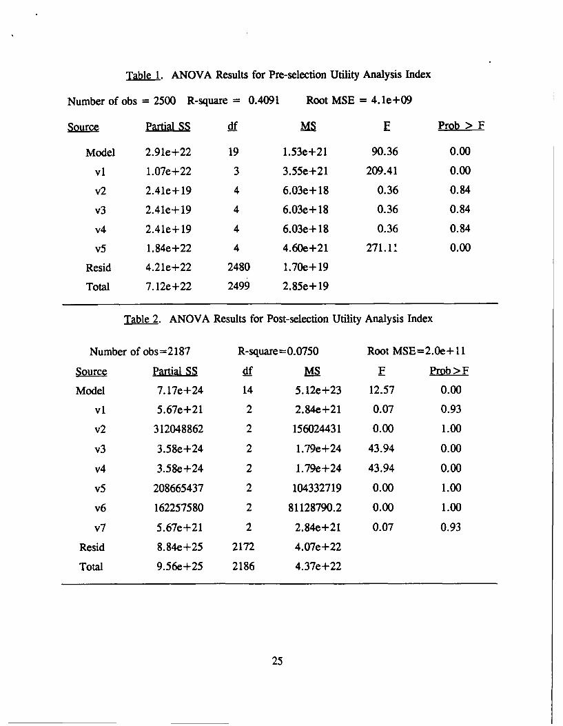
Table 1. ANOVA Results for Pre-selection Utility Analysis Index
Number of obs = 2500 R-square = 0.4091 Root MSE = 4.1e+09
Sourc Partial SS df MS F Prob > F
Model 2.91e+22 19 1.53e+21 90.36 0.00
v1 1.07e+22 3 3.55e+21 209.41 0.00
v2 2.41e+19 4 6.03e+ 18 0.36 0.84
v3 2.41e+ 19 4 6.03e+ 18 0.36 0.84
v4 2.41e+19 4 6.03e+ 18 0.36 0.84
v5 1.84e+22 4 4.60e+21 271.11 0.00
Resid 4.21e+22 2480 1.70e+ 19
Total 7.12e+22 2499 2.85e+ 19
Table 2. ANOVA Results for Post-selection Utility Analysis Index
Number of obs=2187 R-square=0.0750 Root MSE=2.0e+ 11
Source Partial SS df MS F Prob > F
Model 7.17e+24 14 5.12e+23 12.57 0.00
vI 5.67e+21 2 2.84e+21 0.07 0.93
v2 312048862 2 156024431 0.00 1.00
v3 3.58e+24 2 1.79e+24 43.94 0.00
v4 3.58e+24 2 1.79e+24 43.94 0.00
v5 208665437 2 104332719 0.00 1.00
v6 162257580 2 81128790.2 0.00 1.00
v7 5.67e+21 2 2.84e+21 0.07 0.93
Resid 8.84e+25 2172 4.07e+22
Total 9.56e+25 2186 4.37e+22
25

Cost Benefit Analysis
An analysis was also performed for cost/benefit analysis using the following inputvariables and respective values:
vl: Probability of implementation: 0.1, 0.4, 0.7, and 1.0v2: Potential payoff of the project: 5, 25, 50, and 75 (in thousands of dollars)v3: Scope of the problem: 1, 3, 6, and 8v4: DoD objective: 1, 3, 6, and 8v5: Cost estimate: 5, 25, 50, and 75 (in thousands of dollars)v6: Certainty of cost estimate: 1, 4, and 6.
The values assigned to each of the 6 variable inputs produced 3072 combinations of the 6values. Thus, 3076 runs of the cost/benefit analysis model were made in order toevaluate the effect of the six input values. These combinations of values resulted in thefollowing distribution of the cost/benefit analysis index values:
Percentiles Index Values
1% 7815% 516910% 16629.425% 82774.350% 707216.575% 391739090% 796456695% 972662299% 1.4 1e+07
The ANOVA of the cost/benefit analysis index, shown in Table 3, indicated that threeof the six input variables were statistically significant at explaining the variation in the index:potential payoff, DoD objective, and cost estimate.
26

Table 3. ANOVA Results for Cost/Benefit Analysis Index
Number of obs = 3072 R-square = 0.6867 Root MSE = 1.9e+06
Sou~r. Partial SS df MSF Prob > F
Model 2.4347e+ 16 17 1.4322e+ 15 393.84 0.0000
V1 1.5108e+10 3 5.0361e+09 000.00 0.9986
v2 6.4201e+ 15 3 2.1400e +15 588.49 0.0000
v3 8.6859e+ 10 3 2.8953e+ 10 000.01 0.9962
v4 9.7697e+ 15 3 3.2566e+ 15 895.54 0.0000
v5 8.1450e+ 15 3 2.7150e +15 746.61 0.0000
v6 1.2421e+13 2 6.2104e +12 001.71 0.1814
Resid 1. 1106e +16 3054 3.6364e+12
Total 3.5453e+ 16 3071 1. 1544e +13
Decision Analysis
For the computation of the decision analysis index, 12 input variables were used:
vi: State of the art: 0Oand 1v2: Expert availability: 0 and 1v3: Time to complete: 20 and 60v4: Time certainty: 3 and 7v5: Persons availability: 0 and 1v6: Funds availability: 0 and 1v7: Imiplementation probability: 0.3 and 0.8v8: Potential payoff: 20 and 60v9: Problem scope: 3 and 7vlO: DoD objective: 3 and 7v 11: Cost estimate: 20 and 60v12: Cost certainty: 2 and 5
27

Two values were assigned to each of the 12 variable inputs, thus producing 212 or 4096combinations of the 12 values. Thus, 4096 runs of the decision analysis model were made inorder to evaluate the effect of the input values. These combination of values resulted in thefollowing distribution of decision analysis index values:
Percentiles Index Values
1% 13.35% 16.710% 18.925% 27.350% 33.675% 54.290% 65.8195% 74.2699% 79.21
The ANOVA of the decision analysis index, shown in Table 4, indicated that eight ofthe 12 input variables were statistically significant at explaining the variation in the index.The four factors which were not statistically significant were state of the art, expertavailability, persons availability, and funds availability.
28

Table 4. ANOVA Results for Decision Analysis Index
Number of obs = 4096 R-square = 0.9106 Root MSE = 5.30166
PartialSS F Prob > F
Model 1169031.49 12 97419.29 3465.94 0.00
v1 4.78 1 4.78 0.17 0.68
v2 4.78 1 4.78 0.17 0.68
v3 624298.51 1 624298.51 22211.00 0.00
v4 399537.38 1 399537.38 14214.55 0.00
v5 3.09 1 3.09 0.11 0.74
v6 3.09 1 3.09 0.11 0.74
v7 1135.45 1 1135.45 40.40 0.00
v8 1373.54 1 1373.54 48.87 0.00
v9 10210.47 1 10210.47 363.26 0.00
vio 10210.47 1 10210.47 363.26 0.00
vi 70475.65 1 70475.65 2507.35 0.00
v12 51774.31 1 51774.31 1842.00 0.00
Resid 114763.45 4083 28.11
Total 1283794.94 4095 313.50
Comparison of Output of Each Technique
In addition to the sensitivity analysis, a comparison of the output of each technique
was performed. The question being examined in this comparison was how similar were the
results from using each of the four techniques across the 30 simulated projects? Rank order
correlations were used because the values for the input variables were subjectively selected
from a range of possible values; thus, the actual utility or payoff from undertaking any given
simulated project should not be directly compared with that of any other project. The rank
orders from the 30 projects are also shown in Appendix C.
Table 5 shows the rank order correlations for the four techniques. Only the rank
ordered outputs from utility analysis and production functions and from cost/benefit analysis
and decision analysis were statistically different from 0.0 at the .01 level of significance.
29

The latter is readily understandable since a significant portion of the decision analysis
hierarchy is composed of the entire cost/benefit decision hierarchy. An explanation for the
relationship between utility analysis and production functions may be the fact that both
techniques have estimates of the productivity of labor in each project.
Table 5. Rank Order Correlations
UA PF CBA DA
Utility Analysis (UD) 1.00
Production Functions (PF) .52" 1.00
Cost/Benefit Analysis (CBA) -.02 .18 1.00
Decision Analysis (DA) -.09 -. 12 .61 1.00
Significant at .01 level
Although this comparison was done on simulated projects, with data on real projects,
using each technique to estimate the value and costs of conducting each project and
comparing the output from each technique could be very valuable. An MPT R&D resource
allocation decision maker could average across the four techniques as well as investigate
through further sensitivity analysis why similarities or differences might exist. Such analysis
should provide greater insight into the MPT R&D decision process and result in more
effective use of limited R&D resources.
30

Discussion
Utility Analysis
The ease in using utility analysis comes in its pre-defined equations. The model is
already specified regardless of the type of application. However, utility analysis was
developed specifically for selection tests, or for intervention devices in which productivity
can be measured before and after the intervention.
For even the purest selection test, several problems arise in applying utility analysis.
Although the variables fit neatly into an equation, the values assigned to those variables are
difficult to obtain. Matthews et al., (1990) discuss some of the major problems with utility
analysis. Several essential elements are necessary for the estimation of utility (U). First, the
value for standard deviation (SDy) is approximated using an approach suggested by Schmidt,
Hunter, McKenzie, & Muldrow (1979). The estimation of SDy presumes a defensible
method for approximating the dollar value of productivity. The measurement of job
performance in the Air Force is an ongoing area of research in which any selected measure
requires caution in its application to a utility analysis. The calculation of SDy, given a sound
methodology for measuring job performance, is still an approximation to be used with
caution. The value for d, suffers from the same problems.
Second, the validity coefficient is not only dependent on the measurement of
performance but also on the credibility of the coefficient. The correlation between
performance and the device, (r,), involves direct measurements of performance. To the
extent that measures of performance are invalid, utility analysis based on them is
questionable. In the case of the 30 projects, performance measures were unavailable, so
utility analysis suffers greatly. Moreover, there are other factors that explain the individual
variation in salary that, when left out of the benefit algorithm, leave biased estimates of the
worth of a selection or intervention device. This is illustrated even assuming that
performance can be reflected in dollars. Third, additional factors such as personnel turnover
and probability of program success should also become an integral part of the utility analysis.
31

One major problem with the utility benefit formulation is the strong possibility of an
omitted variable bias. For example, economic research has suggested that other variables
such as experience and education are important in explaining the salary variation across
individuals. In this context, if a test score is positively correlated with factors such as
experience, and education, and these variables are excluded from the estimating equation, the
coefficient on test score is overestimated by capturing the effects of some of the omitted
variables.
It is necessary to clarify the relationship between utility analysis and cost benefit
analysis. Whereas cost benefit analysis is an approach to looking at a utility as some net
benefit, utility analysis specifically defines the benefits and costs with an equation. Utility
analysis, then, is really a specific example, or subset, of cost benefit analysis.
Utility analysis could potentially be very useful to decisions concerning pre- and post-
selection tests. However, more research must be conducted on the data that is required to
estimate values for the variables. Estimations by subject matter experts are a possible
solution for some of the variables, such as the number of individuals tested or the cost to
administer the test to an individual. The final values for utility can be found in Appendix C.
Production Function
Like utility analysis, the ease in using the production function comes in its structured
model specifications. However, several problems surface in the attempt to measure the
benefits (output) of MPT R&D at the project level. Quantifying the output of MPT R&D
projects is not obvious, even though surrogates are available at the aggregate level and each
project has assigned deliverables. Literature tends to use measures such as value-added and
total revenues which are not available for MPT R&D. Total expenditures do not measure
benefits, because all projects are not successful; and an expensive project may or may not be
as beneficial to the military as a less expensive project. The dollar size of the research
budget for an individual project may have little bearing on the extent of benefit to the Air
Force. Measuring the inputs also presents a challenging problem, although factors such as
man-hours, contribution to capital, profit, and travel costs may be available from the
proposed project budgets.
32

The key issue is deriving an unbiased measure of output for each project. In
addition, a particular MPT R&D project is not independent of previous research, so theproblem of determining a methodology to capture the contribution of past research to the
present project may not be trivial. Also, MPT R&D performed by the Air Force is not
independent of research performed by other branches of the military. In fact, several joint
research committees exist to take advantage of research performed across the branches of
service.
Research in MPT does not always lead to the generation of a useful product,
especially with respect to basic research. Projects can often be assigned probabilities of
success, though numerous factors such as the level of funding, number of participating
specialists, and level of previous pertinent research can affect the outcome of a project
beyond the feasibility of the statement of work. The failure of a project does not imply that
research in the particular area of interest is not beneficial or useful to the Air Force mission
of national defense. The research attempts which seemingly fail to achieve their initial
objectives are often necessary learning stages and/or adaptations to changing technology in
the process of producing a useful end product, Thus, the key issues are the direction of
basic and applied MPT R&D given the short and long term needs of the Air Force and the
expected return from the allocation of these funds in selected areas of MPT research.
Due to the problems discussed above, it is difficult to actually quantify the
contribution to output of the capital, labor, and R&D stock; however, given the data for the
variables, the production function does yield a ranking of the projects. The final values for
utility can be found in Appendix C.
Cost Benefit Analysis
Applying cost benefit analysis to the 30 MPT research projects proved to be an
effective methodology for this type of analysis. By expanding the general idea of benefitsminus costs to incorporate the relationships among the attributes in MPT projects, a
seemingly reliable ranking of the projects was achieved. The final values for utility can be
found in Appendix C.
The resulting figure for overall utility is a dollar amount. This number seeminglyplaces an actual dollar value on a project. However, the resulting dollar figure is only as
33

valid as the dollar figures input in the equations. Therefore, the value for final utility mustnot be taken too literally. The value does provide a valid means for ranking a set of projectsagainst each other.
There are, however, several issues which complicate the CBA procedure. Theseinclude the selection of the appropriate decision rule for selecting the most beneficial project,uncertainty associated with outcomes or costs, and evaluation of future benefit and costflows. The central issue in applying CBA to research and development is the difficulty inthe identification and valuation of benefits and costs.
Net Benefits Versus the Benefit to Cost Ratio. In the literature on project selection, it issometimes the case that a variant of the CBA methodology, the benefit to cost ratio method,is proposed (Paolini & Glaser, 1977). In this method, a project is recommended because itsbenefit to cost ratio (total benefits divided by total cost) is greater than one, or it is rejectedbecause the ratio is less than one. It may also be adopted because the project has the largestbenefit to cost ratio among competing projects. In many circumstances the benefit to costratio criterion leads to the same choice as maximization of net benefits. However, when achoice must be made among mutually exclusive projects or when resources are constrained,the two criteria may lead to inconsistent choices. To understand how the benefit to cost ratiocan be misleading, suppose a policy maker is considering two alternative research anddevelopment projects. CBA produces estimates as follows:
Benefit/Project Benefits Costs Net Benefits Cost Ratio
I $ 10,000 $ 1,000 $9,000 10.0
II $100,000 $25,000 $75,000 4.0
In this situation, Project I has a higher benefit to cost ratio, while Project II has larger
net benefits. In the example, if the decision maker is maximizing net benefits on a projectby project basis, Project II is preferred; but, if the decision rule is to maximize the benefitper unit of cost, then Project I is the clear choice. If the level of effort could be increased inProject I to $25,000 with the benefit to cost ratio constant, then the apparent ambiguitybetween the decision rules would disappear.
34

Uncertainty in the Environment. In striving for more accurate estimates of benefits andcosts, complications are introduced into the analysis. For example, there may be uncertaintyabout the exact magnitude of the benefits but relative confidence in the probability of theiroccurrence. In this instance, the benefits can be multiplied by their respective probabilitiesand summed to produce a value for benefits which is a weighted average based on theirexpected probability of occurrence. Suppose there are three estimates of the benefits of aparticular project: $100,000, $80,000 and $60,000 with estimates of the probability thateach will occur of, respectively, 20%, 50%, and 30%. The project would have an expectedbenefit of
(0.2 * $100,000) + (0.5 * $80,000) + (0.3 * $60,000) = $78,000,
which would be used as the total benefits in the analysis. In this example, only three discreteamounts are estimated. More likely, the analyst will have a continuous range within whichthe benefits are expected to fall and as estimate of the frequency distribution of the benefitsover this range. Thus, CBA employing expected values has a more complicated computationof the expected benefits than CBA in a certain environment.
Evaluating the Flow of Future Returns and Costs. Another important modification is therecognition that both benefits and costs may occur overtime. Using standard discountingtechniques to establish equivalent present values, the relative attractiveness of differentprojects can be compared. The results, however, are sensitive to the discounting procedure.
For example, a cash flow of $1,000 in one year, $3,000 in two years, and $5,000 in threeyears, using an interest rate of 10%, would have a present value of
[$1,000/1.1] + [$3,000/(1.1)2 ] + [$5,000/(1.1) ] = $7,144.
Hodder and Riggs (1985) illustrate how discounting techniques tend to favor near-term,incremental contributions over longer-term, but presumably larger advances. In particular,the discount rate should consist of three components: a risk-free time value of money, apremium for expected inflation, and a premium for the risk of project failure. Instead,applications typically apply a single, undifferentiated discount rate for all three componentsand thus heavily penalize the future on the grounds that it is inherently less certain. Inaddition, the level of uncertainty associated with a typical R&D program should decrease asprogress is made, and therefore the program risk premium should vary from one stage to thenext. If the future cash flows are adjusted for their changing risk premium, the final result
35

may be quite different from an unadjusted estimation. Thus, the need to separate timediscount and risk adjustment factors and to vary the latter for different stages of the programis recognized in the literature. Unfortunately, according to Hodder and Riggs (1985), thisneed is generally ignored in practice.
The choice of an appropriate discount rate is essential in reference to MPT R&D.
The funds expended for a government project are not funds that would otherwise stand idle.They are obtained by the government from the private sector, either by taxation orborrowing. If these funds were left in the private sector, they would be put to use there andwould earn a rate of return that measures the value that society places on that use of thefunds. If the funds are diverted to government use, the true cost of the diversion is thereturn that would otherwise have been earned. This opportunity cost is the correct discountrate to use in calculating the present value of a proposed project. Most economists who areconcerned with determining the appropriate discount rate for public projects use a figure ofabout 10 percent.
Valuation of Benefits and Costs. By far the most difficult issue in CBA is how to actuallyplace a value on benefits and costs. The methodology used for the valuation of costs and
benefits is not standardized across studies but is adjusted depending on the characteristics orattributes of the program or venture being reviewed. Some benefits, and especially somecosts, are straightforward and easily calculated. In MPT research, though, there are farmore intangible benefits and costs. One way to calculate benefits is the valuation of AirForce experience (Stone et al., 1989). This methodology incorporates human capital andhuman resource accounting techniques to quantify such benefits as reduced attrition,increased retention, and improved training effectiveness. The valuation of Air Forceexperience could be incorporated into a computer simulation model, and allow the benefit
calculation to be done by aging the manpower force through several years, accounting forsome change in retention or attrition due to the impact of a personnel policy change. Thispolicy change would be attributable to the benefit of an MPT R&D project.
Decision Analysis
Decision analysis is a systematic and structured methodology for the purpose of aiding
in the decision-making process. It is not designed to be an exact model of the decision-making process, but a consistent method with which to attack all decisions of a particular
36

type. Keeping this in mind, decision analysis proves to offer consistency and validity toMPT R&D decisions. As with each of the above methodologies, there are pros and cons toapplying decision analysis in the research context.
The final value for utility in decision analysis is a standardized number. In this case,it is a number from 1 to 100. Therefore, this final utility does not place an actual value on aparticular project. The single number tells the decision-maker nothing about the value of theproject. However, in the context of competing projects, the final value describes the relativeworth of the projects. Therefore, decision theory is useful in ranking the projects against
each other. The final values for utility can be found in Appendix C.
Another issue involved in decision theory is the attributes to be evaluated. There areseveral more variables than in any of the other methodologies we have explored. In general,the attributes are also considerably more subjective. On one hand, this makes the data mucheasier to attain. Decision makers need only to fill in their estimates on many of theattributes. In addition, the number of attributes tends to remove some of the emphasis offthe cost and benefit estimates which are often uncertain. On the other hand, this makes thedata far less reliA ,-. It may be difficult to reach a consensus among several individuals onhow so many attrit',.es should be rated and weighted.
Accumulation of Data. Ideally, the decision maker should have all the data necessary to rankthe projects available. Although much of the data can be difficult to attain, the resourceallocation manager can increase the accuracy of the evaluation of the project by supplyinguseful as well as descriptive information to the decision makers. Considering the variablesnecessary for the techniques described above, that data can be summarized in this proposedformat for a request for personnel research. Of course, the more quantified is the datasupplied, the more useful it will be to the decision maker.
V. CONCLUSIONS AND RECOMMENDATIONS
This report compared four techniques for their usability in the measurement of benefitsof MPT research and development. Utility analysis was most useful in measuring thebenefits of selection tests or other intervention devices in which productivity of the worker
37

can be measured before and after the intervention. In other MPT R&D efforts, utilityanalysis has limited practical applicability. Production function methodologies were notapplicablc to the individual R&D project problem. It was difficult to quantify thecontribution to output of the various input variables.
Cost benefit analysis was found to have practical application to the R&D projectproblem. The family of techniques was specifically developed for the problem of comparingalternative plans, for which the cost and benefit of each plan could be measured. Theproblem with cost benefit analysis was that the user must decide on a way in which tomeasure the costs and benefits associated with an individual R&D project. For test devices,utility analysis was a useful tool for determining the costs and benefits associated withdeveloping the test. For other types of MPT R&D projects a computer simulation modelincorporating human capital, human resource accounting, and productivity measurement toolswould be an extremely useful tool for developing estimates of costs and benefits.
Decision analysis was also found to have practical applications to the MPT R&Dselection context. In general, however, the results were more subjective than the cost benefitapproach, since the data collection effort was primarily concerned with expert judgmentsrather than costs and benefits. Decision analysis was found most useful in rank orderingR&D projects, rather than in measuring the benefit of R&D projects.
The ANOVA indicated that not all of the respective input factors were equallyimportant in explaining the variation in the three output variables. In many cases inputvariables were difficult, if not impossible, to measure or obtain. However, if such variableswere statistically unimportant, then the use of the technique was not significantly hamperedby the lack of accuracy in the estimation of the input variable. Conversely, if a difficult-to-obtain input variable was statistically important to the use of the technique, then the use ofthe technique was severely limited for lack of creditable input data.
Based on these results and conclusions a prototype functional software package wasdeveloped. This package incorporated the best points of the techniques, forming a modelsuitable for the MPT R&D context.
There are many ways in which this prototype model is flexible to change, but oneparticular flexibility would be most beneficial. In addition to the user having the option to
38

choose data, model specifications, and benefit calculations, the option to change the structureof the basic hierarchy would open new doors for such a package. If this characteristic wasdeveloped, the package could be applied to a much wider range of research topics.Continued research in this area, then, could potentially be quite beneficial.
39

REFERENCES
Buudreau, J.W. (1983). Economic considerations in estimating the utility of human resourceproductivity improvement programs. Personnel Psychology.
Brodgen, (1949). When testing pays off. Personnel Psychology.
Cascio, W.F. (1991). Costing Human Resources: The Flnalncial Impact of Behavior inOrganizations. Boston, MA: PWS-Kent Publishing Company.
Clark, K.B. & Griliches, Z. (1984). Productivity growth and R&D at the business level:results from the PIMS data base. In R&D. Patents. and Productivity, edited by ZviGriliches. University of Chicago Press, Chicago, Illinois.
Cronbach, L.J., & Gleser, G.C. (1965). Psychological Tests and Personnel Decisions.Champaign, II: University of Illinois Press.
DeVany, A.S., Gramm, W.L., Saving, T.R., & Smithson, C.W. (1983). Production in aservice industry using customer inputs: A stochastic model. Review of Economicsand Statistics.
Fast, J.C. & Looper, L.T. (1988). Multiattribute decision modeling techniques: Acomparative analysis (AFHRL-TR-88-3). Brooks AFB, TX: Manpower andPersonnel Division, Air Force Human Resources Laboratory.
Fast, J.C., Taylor, J.T., & Looper, L.T. (1991). The integrated decision modeling system(IDMS) user's manual. (AL-TP-1991-0009) Brooks AFB, TX: Manpower andPersonnel Research Division, Human Resources Directorate, Armstrong Laboratory.
Griliches, Z. (1987, July). R&D and productivity: Measurement Issues and Econometricresults. Science.
Griliches, Z. (1986, March). Productivity, R&D, and basic research at the firm level in the1970's. American Economic Review.
Griliches, Z. (1984). Productivity and R&D at the firm level. In R&D. Patents. andProductivity, edited by Zvi Griliches. University of Chicago Press, Chicago, IL.
Henderson, J.M., & Quandt, R.E. (1958). Microeconomic Theory: A MathematicalApproach. McGraw-Hill Book Company, New York.
Hodder, J.E., & Riggs, H.E. (1985, January-February). Pitfalls in evaluating risky projects.Harvard Business Review, pp. 128-136.
40

Hunter, J.E., & Schmidt, F.L. (1983). Quantifying the effects of psychological interventions
on employee job performance and work-force productivit, American Psychologist.
Irvine, J. & Martin, B.R. (1983). Assessing basic research. Social Studies of Science.
Jaffe, A.B. (1986, December). Technological opportunity and spillovers of R&D: evidencefrom firm's patents, profits, and market value. American Economic Review.
Kmenta, J. (1971). Elements of Econometrics. Macmillan Publishing Co., Inc., New York.
Mansfield, E. (1980). Basic research and productivity increase in manufacturing. AmericanEconomic Review.
Matthews, M.D., Looper, L.T., & Engquist, S.K. (1990). Application of utility models tothe evaluation of military manpower and personnel research programs: A criticalreview and illustrations (AFHRL-TP-90-54). Brooks AFB, TX: Manpowcr andPersonnel Division, Air Force Human Resources Laboratory.
Paolini, A. Jr. & Glaser, M.A. (1977, May). Project selection methods that pick winners,Research Management, pp. 26-29.
Reinhardt, U. (1972, February). A production function for physician services. Review ofEconomics and Statistics.
Schmidt, F.L., Hunter, J.E., McKenzie, R.C., & Muldrow, T.W. (1979). Impact of validselection procedures on work-force productivity. Journal of Applied Psychology.
Stevenson, R. (1990). Front end analysis guidlines (AFHRL-TP-90-35). Brooks AFb, TX:Manpower and Personnel Division, Air FOrce Human Resources Laboratory.
Stone, B.M., Rettenmaier, A.J., Saving, T.R., & Looper, L.T. (1989). Technology toAssess the Value of Air Force Experience. Forthcoming technical paper. BrooksAFB: Manpower and Personnel Division, Air Force Human Resources Laboratory.
Taylor, H.C., & Russell, IT. (1939). The relationship of validity coefficients to thepractical effectiveness of tests in selection: Discussion and tables. Journal of AppliedPsychology.
Von Winterfeldt, D., & Edwards, W. (1986). Decision analysis and behavioral research,Cambridge University Press.
Zellner, A., Kmenta, J., & Dreze, J. (1966, October). Specification and estimation ofCobb-Douglas production function models. Econometrica.
41

APPENDIX A
SIMULATED DATA FOR FOUR TECHNIQUES
Utility Analysis Data - Pre-Selection
N, R W851W50/W15 MNC
Project 1: 55,000 .12 10,000/8,000/3,000 .62 100Project 2: 25,000 .3 12,000/8,000/4,000 .55 150Project 3: 10,000 .4 5,000/2,000/1,000 .4 200Project 4: 25,000 .53 8,000/6,000/2,000 .63 150Project 5: 55,000 .4 12,000/8,000/6,000 .88 500Project 6: 5,000 .09 6,000/4,000/1,500 .72 100Project 7: 40,000 .15 18,000/12,000/2,000 .81 200Project 8: 15,000 .77 15,000/10,000/5,000 .88 250Project 9: 40,000 .9 19,500/12,000/4,000 .77 25Project 10: 20,000 .75 18,000/12,000/6,000 .75 120Project 11: See post-selectioaProject 12: 30,000 .35 17,500/13,500/11,500 .70 130Project 13: See post-selectionProject 14: 50,000 .25 10,000/6,000/2,000 .6 75Project 15: See post-selectionProject 16: 50,000 .19 8,200/5,100/4,300 .81 55Project 17: 15,000 .78 22,000/17,000/15,000 .9 485Project 18: 55,000 .66 12,000/6,000/3,200 .7 25Project 19: 2,000 .85 25,000/17,000/5,000 .8 55Project 20: 15,000 .25 25,000/17,000/5,000 .8 50Project 21: 12,000 .38 12,000/8,000/6,000 .78 20Project 22: 2,000 .4 12,000/8,000/6,000 .64 100Project 23: 48,000 .45 18,000/17,290/15,480 .42 75Project 24: 55,000 .67 20,000/16,000/8,000 .75 35Project 25: 10,000 .33 10,000/5,000/2,000 .6 25Project 26: See post-selectionProject 27: 20,000 .55 40,000/31,000/22,000 .8 120Project 28: 8,000 .21 9,000/6,000/3,000 .84 28Project 29: 20,000 .64 40,000/31,000/22,000 .8 150Project 30: 50,000 .78 8,000/6,000/4,000 .78 80
42

Utility Analysis Data - Post Selection
MN MN D
Project 11: 45,000 .7 .4 .03 .21 100Project 13: 35,000 .89 .51 .023 .3 400
Project 15: 55,000 .85 .35 .04 .45 70
Project 26: 20,000 .72 .5 .03 .75 1,000
43

Production Function Data
Capital (M) Labor (M) R&D Stock (M)
Project 1: 2 1 .250Project 2: 3 2 5Project 3: 1 1 1Project 4: 1 1 1Project 5: .5 1.5 1Project 6: 5 5 0Project 7: 3 2 0Project 8: 2 1 2Project 9: 2 4 5Project 10: 10 10 20Project 11: 15 15 1Project 12: 1 3 5Project 13: 3 7 2Project 14: 3 5 3Project 15: 4 6 10Project 16: 2 2 3Project 17: 1 1 0Project 18: .5 1.5 15Project 19: 2 8 4Project 20: 2 3 5Project 21: 2.5 2 0Project 22: 2 8 5Project 23: 2 3 1Project 24: 5 10 20Project 25: .5 1.5 3Project 26: 10 20 1Project 27: 3 4 3Project 28: 5 5 10Project 29: 5 15 10Project 30: 1 2 15
44

Decision Analysis Data
State Expert Time to Time Person Fundsof Art Avail CompI Cert Avail Avail
Project 1: 1 1 24 5 1 1Project 2: 1 1 60 6 1 1Project 3: 1 1 24 6 1 1Project 4: 1 1 36 7 1 1Project 5: 1 1 20 3 1 1Project 6: 1 0 36 2 1 1Project 7: 1 0 30 4 1 1Project 8: 1 1 48 3 1 1Project 9: 1 1 24 5 1 1Project 10: 1 1 36 7 1 1Project 11: 0 0 48 8 0 0Project 12: 1 1 18 6 1 1Project 13: 1 1 50 5 1 1Project 14: 1 1 60 8 1 1Project 15: 1 1 60 8 1 1Project 16: 1 1 42 6 1 1Project 17: 1 1 42 7 1 1Project 18: 1 1 24 5 1 1Project 19: 1 1 42 7 1 1Project 20: 1 1 27 6 1 1Project 21: 1 1 9 6 1 1Project 22: 1 1 36 6 1 1Project 23: 1 1 60 7 1 1Project 24: 1 1 24 4 1 1Project 25: 1 1 12 6 1 1Project 26: 1 1 45 5 1 0Project 27: 1 1 24 3 1 1Project 28: 1 1 52 5 1 1Project 29: 1 1 42 6 1 1Project 30: 1 1 30 7 1 1
45

Decision Analysis Data: Part 2 (Also CBA)
Impi Pot Prob DoD Cost CostProb PaScye ObjDec Estim Cert
Project 1: .8 10 4 6 5 6Project 2: .9 20 5 5 10 6
Project 3: .85 25 3 5 3 7
Project 4: .8 15 4 5 3 7Project 5: .75 15 6 7 2 3Project 6: .3 30 4 5 10 3
Project 7: .4 20 2 6 5 4
Project 8: .6 30 3 6 3 5
Project 9: .5 18 4 3 4 2
Project 10: .85 40 5 7 20 4
Project 11: .6 60 3 5 30 6
Project 12: .95 20 6 6 4 3Project 13: .7 35 4 6 10 2
Project 14: .93 40 7 7 8 3Project 15: .98 30 7 7 10 3
Project 16: .8 10 6 5 4 2
Project 17: .6 40 2 8 2 2
Project 18: .92 30 7 7 2 7
Project 19: .75 50 4 7 10 3Project 20: .35 40 4 5 5 4
Project 21: .5 15 5 5 3 5
Project 22: .95 50 8 7 10 4
Project 23: .4 25 6 6 5 2
Project 24: .85 30 7 5 15 3Project 25: .8 20 3 3 2 3Project 26: .65 60 2 6 30 5
Project 27: .78 35 4 6 7 4
Project 28: .4 40 4 5 10 2Project 29: .35 45 2 7 20 4Project 30: .45 30 7 7 15 3
46

APPENDIX B
MODEL SPECIFICATIONS
Decision Analysis
F1 = 40x, + 60x2 ; Technical Capability
F2 = 31.429 - .64292x3 + 8.571x 4 - .0238x3x4 ; Timeliness
F3 = 20x5 + 30x6 + 50x5x6 ; Resources
F4 = lOx7 + .5x8 + x7xg ; Product Value
F5 = -14.286 + 4.286x9 + lx 10 ; Utility to DoD
F6 = 54.2870 - .9524x,, + 5.713x12 - .0476xtxt2 ; Price Stability
x, = State of the Art
X2 = Expertise Availability
X3 = Time to Complete
X4 = Certainty of Time Schedule
X5 = Personnel Availability
=X = Funds Availability
X7 = Implementation Probability
x, = Expected Payoff
x9 = Problem Scope
xto = DoD Objective
x1 = Cost Estimate
x12 = Certainty of Cost Estimate
47

Ranks and Weights for Decision Analysis:
Rank Weight (1-100)
Technical Capability 1 100
Timeliness 3 75
Resources 2 80
Rank Weight (1-100)
Product Value 1 100
Utility to DoD 290
Rank Weight (1-100)
Feasibility 2 80
Benefits 1 100
Costs 3 75
48
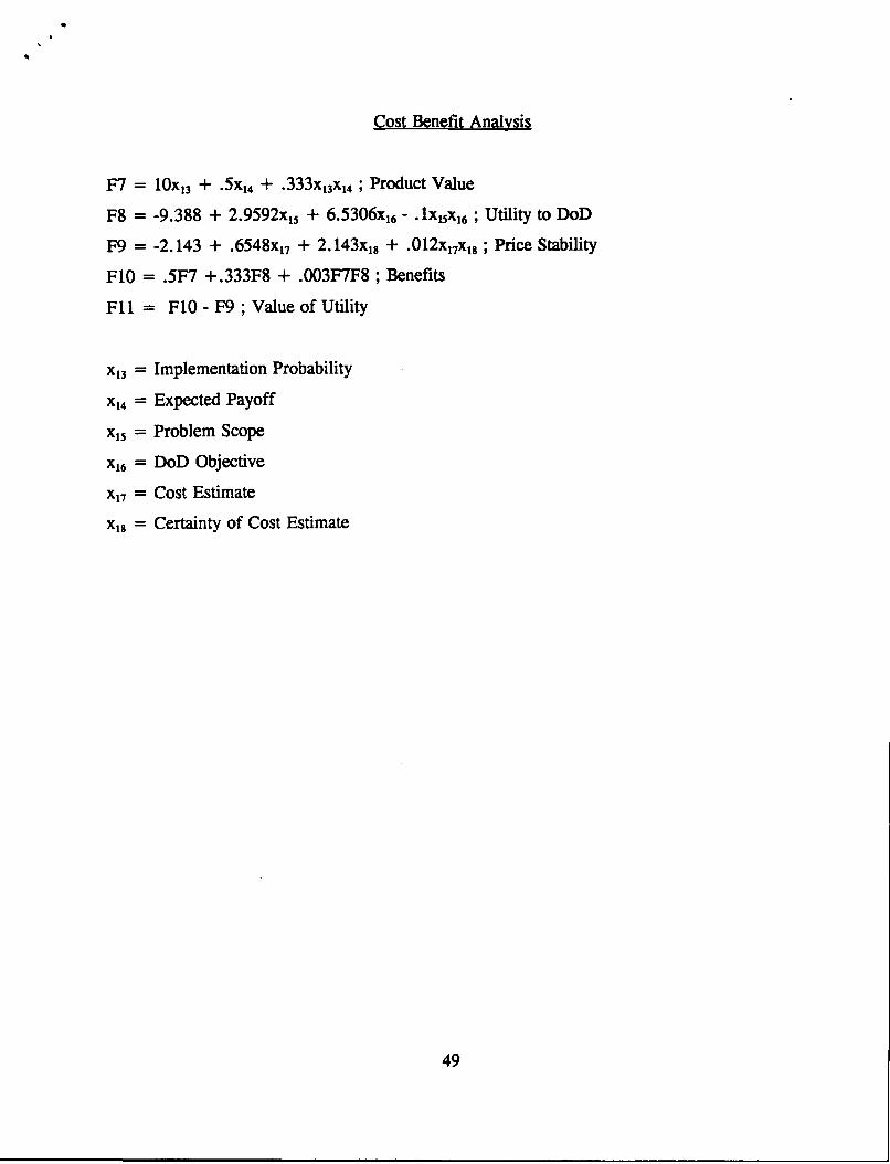
Cost Benefit Analysis
F7 = 1OX13 + .5x, 4 + .333x 13X14 ; Product Value
F8 = -9.388 + 2.9592x, 5 + 6.5306x16 - l15Xx16 ; Utility to DoD
F9 = -2.143 + .6548x, 7 + 2.143x18 + .012x17X18; Price Stability
F10 = .5F7 +.333F8 + .003F7F8 ; Benefits
Fll = F10- F9 ;Valueof Utility
X3= Implementation Probability
X4= Expected Payoff
X5= Problem Scope
X6= DoD Objective
X7= Cost Estimate
x8= Certainty of Cost Estimate
49

APPENDIX C
FINAL VALUES FOR UTILITY
Utility Production Cost Benefit DecisionAnalysis Functions Analysis Analysis
Project 1: 14,960,000(18) 955,028(24) 839,000(28) 67.55(12)Project 2: 12,750,000(20) 2,142,791(15) 902,000(27) 66.10(18)Project 3: - 400,000(30) 883,079(26) 1,175,000(22) 72.39(5)Project 4: 29,640,000(15) 883,079(27) 763,000(29) 69.98(9)Project 5: 11,220,000(22) 924,681(25) 2,312,000(9) 67.01(15)Project 6: 310,000(29) 1,102,734(22) 1,241,000(21) 45.21(29)Project 7: 40,600,000(13) 542,964(28) 1,161,000(24) 49.49(28)Project 8: 47,070,000(12) 1,149,188(21) 1,805,000(16) 66.50(16)Project 9: 220,760,000(4) 3,499,859(12) 1,164,000(23) 56.26(26)Project 10: 65,100,000(10) 9,200,081(3) 2,097,000(12) 71.09(7)Project 11: 1,959,461,012( 2)* 10,158,610(2) 609,000(30) 44.54(30)Project 12: 10,800,000(23) 1,994,019(17) 2,391,000( 8) 69.42(10)Project 13: 1,886,359,134( 3)* 4,246,086(10) 2,431,000(7) 63.52(20)Project 14: 28,750,000(16) 3,584,072(11) 3,492,000( 2) 74.84(3)Project 15: 2,045,878,979( 1)* 4,848,974( 6) 2,887,000( 5) 71.65(6)Project 16: 3,406,000(27) 1,819,670(18) 1,742,000(18) 60.59(24)Project 17: 13,785,000(19) 258,226(30) 3,402,000( 3) 70.27(8)Project 18: 69,773,000(9) 1,176,695(20) 2,495,000(6) 80.90(1)Project 19: 16,210,000(17) 4,354,828( 9) 3,253,000( 4) 73.21(4)Project 20: 35,250,000(14) 2,439,659(14) 1,796,000(17) 66.40(17)Project 21: 6,873,600(24) 514,908(29) 1,022,000(26) 67.20(14)Project 22: 824,000(28) 4,442,178(8) 3,803,000(1) 80.15(2)Project 23: 12,038,400(21) 2,114,077(16) 2,163,000(11) 62.62(22)Project 24: 219,175,000(5) 7,519,551(5) 1,871,000(14) 65.07(19)Project 25: 5,690,000(25) 1,019,661(23) 1,332,000(19) 61.61(23)Project 26: 200,162,903( 6)* 10,762,900( 1) 1,134,000(25) 55.53(27)Project 27: 76,800,000(8) 3,127,265(13) 2,296,000(10) 68.70(11)Project 28: 4,009,600(26) 4,628,826(7) 1,967,000(13) 59.66(25)Project 29: 89,160,000(7) 9,057,159( 4) 1,257,000(20) 63.27(21)Project 30: 56,840,000(11) 1,716,332(19) 1,847,000(15) 67.25(13)
* Post-selection intervention device
()Denotes rank order based on final value
50