Working Papers on the Nature of Evidence: How Well Do “Facts” Travel?

No. 13/06

Measuring Instruments in Economics and the Velocity of Money

Mary S. Morgan © Mary S. Morgan Department of Economic History London School of Economics

August 2006

‘facts’

how

“The Nature of Evidence: How Well Do ‘Facts’ Travel?” is funded by The Leverhulme Trust and the E.S.R.C. at the Department of Economic History, London School of Economics. For further details about this project and additional copies of this, and other papers in the series, go to: http://www.lse.ac.uk/collection/economichistory/ Series Editor: Dr. Jon Adams Department of Economic History London School of Economics Houghton Street London WC2A 2AE Email: j.adams1@lse.ac.uk Tel: +44 (0) 20 7955 6727 Fax: +44 (0) 20 7955 7730

Measuring Instruments in Economics and the Velocity of Money

Mary S. Morgan1

Abstract Economic measurements are generated by complicated systems of measurement involving economic and bureaucratic processes. Whether these measuring instruments produce reliable numbers: ‘facts’ that travel well, depends on the qualities of these systems. Ideas from metrology, and from the philosophy and sociology of science, are used to analyse various attempts to measure the velocity of money ranging from the 17th to the 20th centuries. These historical experiences suggest that numerical facts are likely to travel well in economics when the criteria implied by all three of these disciplinary approaches to measurement are met.

Introduction In economics, facts are hard things like numbers: measurements of

unemployment, for example, or of prices or money. Numbers like these that

become widely accepted within the economics community, and are used

without much consideration of how they were found or made, can be

considered as facts that have travelled well. Yet such facts are hard to come

by. This paper considers three different strands of literature which relate the

construction of measuring systems to generate such numbers to their

effectiveness, reliability and trustworthiness in representing the economic

world. This paper looks at the history of one particular kind of numbers -

measurements of the velocity of money - to investigate how these

1 This paper was originally drafted for presentation at “History and Philosophy of Money” Workshop, Peter Wall Institute for Advanced Study, University of British Columbia, 12-14th November 2004. Revised versions were given at the Cachan/Amsterdam Research Day (December 2004), at the ESHET conference in Stirling, (June 2005), at the ANU (October 2005), at the ASSA (January 2006) and at the Workshop on Economic Measurement, Amsterdam, April 2006. I thank participants who commented on these occasions, particularly Malcolm Rutherford David Laidler, Marcel Boumans and Janet Hunter. This version has benefited from thinking about the problem in the context of “How Well Do ‘Facts’ Travel?”, a Leverhulme/ESRC-funded project at the Department of Economic History, LSE. I thank Arshi Khan, Xavier Duran, Sheldon Steed and Bruce McDonald for research assistance; and Peter Rodenburg, Hsiang-Ke Chao and Marcel Boumans for teaching me about measurement in economics. Comments welcome to m.morgan@lse.ac.uk ©Mary S. Morgan, 2006.

1

requirements for good measuring systems might be understood and how they

fit together. The case suggests that numbers produced according to

instruments which have fulfilled the requirements implied by all three

approaches are likely to travel well, while those that fail on one of these

approaches are likely to crumble in our hands when we try to use them.

1. How do we get good measurements of velocity?

How should we measure velocity of money? This is a question which

has intrigued, if not baffled, economists for several centuries. Even William

Stanley Jevons, who proved to be one of the 19th centuries most willing and

innovative measurers in economics, stated:

I have never met with any attempt to determine in any country the average rapidity of circulation, nor have I been able to think of any means whatever of approaching the investigation of the question, except in the inverse way. If we knew the amount of exchanges effected and the quantity of currency used, we might get by division the average numbers of times the currency is turned over; but the data, as already stated, are quite wanting. (Jevons 1909 [1875] p 336).

Nowadays, this is indeed the kind of formula used in measuring velocity: some

version of the values of total expenditure (usually nominal GDP) and of money

stock are taken ready made from “official statistical sources”, and velocity is

measured by dividing the former by the latter. For example, the Federal

Reserve Chart Book routinely charted something it called the “Income Velocity

of Money” in the 1980s, namely GNP/M1 and GNP/M2 (in seasonally adjusted

terms, with quarterly observations on a ratio scale).2

But such treatment accorded to velocity - as taken for granted, easily

measured and charted - does not mean that the problems of adequately

measuring the velocity of money have been solved, or that the Fed’s modern

measurements are any more useful than those of three centuries earlier. Let

me begin by contrasting that standard late 20th century method of measuring

the velocity of money with one from the 17th century.

2

William Petty undertook a series of calculations of the economic

resources of England and Wales in his Verbum Sapienti of around 1665 and

asked himself how much money “is necessary to drive the Trade of the Nation”

having already estimated the total “expence” of the nation to be £40 millions.

This set him to consider the “revolutions” undergone by money:

if the revolutions were in such short Circles, viz. weekly, as happens among the poorer artisans and labourers, who receive and pay every Saturday, then 40/52 parts of 1 Million of Money would answer those ends: But if the Circles be quarterly, according to our Custom of paying rent, and gathering Taxes, then 10 Millions were requisite. Wherefore supposing payments in general to be of a mixed Circle between One week and 13. then add 10 Millions to 40/52, the half of the which will be 5½, so as if we have 5½ Millions we have enough. (Petty, in 1997 [1899], pp 112-3.)

Now Petty set out to measure the amount of necessary money stock given the

total “expenses” of the nation, not to measure velocity, but it is easy to see that

he had to make some assumptions or estimates of the circulation of money

according to the two main kinds of payments. He supposed, on grounds of his

knowledge of the common payment modes, that the circulation of payments

was 52 times per year for one class of people and their transactions and 4 for

the other, and guesstimated the shares of such payments in the whole

(namely that payments were divided half into each class), in order to get to his

result of the total money needed by the economy.

If we simple average Petty’s circulation numbers, we would get a

velocity number of 28 times per year (money circulating once every 13 days);

but Petty was careful enough to realise that for his purpose to find the

necessary money stock, these must be weighted by the relative amounts of

their transactions. Such an adjustment must also be made to find velocity

according to our modern ideas. If we employ the formula that velocity = total

expenditure/money stock, we get a velocity equal 7.3 (or that money circulates

once every 50 days).

One immediate contrast that we can notice between these two episodes

2 For example, 1984 p5, 1986, p8.

3

is that in Petty’s discussion, the original circulation figures for the two kinds of

transaction - the figures relating to velocity - were needed to derive the money

stock necessary for the functioning of the economy and having found this

unknown, it was then possible (though Petty did not do this) to feed this back

into a formula to calculate the overall velocity figure. We used the formula here

to act as a calculation device for velocity, the measurements themselves were

based on independent guesstimates of circulation by Petty. This is in contrast

to the modern way used by the Fed, where their velocity number is derived

from the formula V=GNP/M. This simple model formula acts as the measuring

device for velocity. There are no independent or separate numbers which

constitute direct measurements (or even guesses) of monetary circulation or

velocity.

These two methods of measuring velocity - Petty’s direct way and the

modern derived way - are very different. It is tempting to think that the Fed’s

was a better measure because it was based on real statistics not Petty’s

guess work, and because its formula links up with other concepts of our

modern economic theories. But we should be wary of this claim. We should

rather ask ourselves: What concept in economics does the Fed’s formula

actually measure? And, Does it measure velocity in an effective way? For this,

we need to have some ideas about measurement.

A small warning is in order here lest I be misunderstood: This paper

does not in any sense pretend to be a comprehensive history of all the

attempts to measure the velocity of money. Rather it picks out some particular

contributions which are of interest to two sets of questions, one set about the

constitution of economic measurement and the other about the history of

economists’ attempts to provide measurements for the concepts in their field

and their claims about such numbers. The aim is to show the usefulness of the

concept of measuring instruments in thinking about the history of

measurement in economics.

4

2. Measuring Things

2.1 Ideas about Measuring from Philosophy, Metrology and History

of Science

There are three kinds of literature on measurement that I want to

introduce in relation to measurement of things which don’t seem easy to

measure. These literatures come from three different starting points: namely,

from the philosophy of science, from metrology, and from the social

studies/history of science. But as we shall see, they are complementary rather

than otherwise.

The mainstream philosophy of science position, known as the

representational theory of measurement, is associated particularly with the

work of Patrick Suppes.3 This theory was developed by Suppes in conjunction

with Krantz, Tversky and Luce, and grew, out of their shared practical

experience of experiments in psychology, into a highly formalized approach

between the 1970s and 1990s. The original three volumes of their studies

ranged widely across the natural and social sciences and has formed the

basis for much further work on the philosophy of measurement.

Formally, this theory requires one to think about measurement in terms

of a correspondence, or mapping: a well defined operational procedure

between an empirical relational structure and a numerical relational structure.

Measurement is defined as showing that “the structure of a set of phenomena

under certain empirical operations and relations is the same as the structure of

some set of numbers under corresponding arithmetical operations and

relations” (Suppes, 1998). This theory is, as already remarked, highly

formalized, but informally, Suppes himself has used the following example.4

Imagine we have a mechanical balance - this provides an empirical relational

structure whose operations can be mapped onto a numerical relational

structure for it embodies the relations of equality, and more/less than, in the

positions of the pans as weights are place in them. The balance provides a 3 For the original work, see Krantz et al, 1971. For recent versions see Suppes 1998, and 2002. A more user friendly version is found in Finkelstein, 1974 and 1982.

5

representational model of certain numerical relations, and we can see a

numerical model isomorphic to the empirical model. Though this informal

example nicely helps us remember the role of the representation, and

foresees how the numerical relations can lead to calculation, it is unclear how

you find the valid representation.5

Finkelstein (1982) and Sydenham (1982), both in the Handbook of

Measurement Science, offer more pragmatic accounts to go alongside and

interpret the representational theory’s formal requirements to ensure valid

measurement. Finkelstein’s informal definition talks of the assignment of

numbers to properties of objects, stressing the role of objectivity and that

“measurement is an empirical process, ... the result of observation and not, for

example, of a thought experiment” (Finkelstein p 6-7).

This practical version of the representational theory closes in on the

second approach - which I call the metrology approach - developed for

economics by Marcel Boumans (1999, 2001 and 2005), at the University of

Amsterdam. Boumans’ innovation here entails taking seriously the notion that

we have “measuring instruments” in economics. We may not recognise them

as such, but Boumans shows us that the history of economics is full of

mathematical formulae, models, or even parts of models, that we use as

devices or instruments to enable us to put measurements (ie numbers) to

apparently unmeasurable entities in economics. (This is not a discussion of

econometrics, which seeks measurements of the relations between entities.6)

For Boumans, the bases of successful measurement depend on creating or

developing measuring instruments (formulae) that are, as far as possible,

invariant to changes in environment while at the same time accurately

capturing the variations of the entity being measured. His work shows how

mathematical measuring devices are constructed to fulfill these requirements

4 At his Lakatos award lecture at LSE, 2004. 5 See Rodenburg (2006) on how these representations are found in one area of economics, namely the measurement of unemployment. 6 Chao (2002 and forthcoming) discusses the usefulness of the representational approach and the idea of measuring instruments in understanding econometric models applied to consumption relations.

6

and how economists’ measuring instruments function to overcome standard

problems such as extracting signal from noise, filtering, and calibrating the

signal to numbers.

In parallel to these philosophical and metrological approaches, Ted

Porter (1994 and 1995) in the history of the social sciences, has focussed on

the ways in which social science numbers become accepted as legitimate and

conventional measurements in their fields. In particular, his notion of the

development of “standardized quantitative rules” focuses on the qualities

necessarily for social science numbers to count as “objective”. All three named

elements contribute to our willingness to have “trust in numbers”, that is to

think of them as being “objective” measurements. “Quantitative” refers to a

level of precision and exactitude we associate with the notion of measurement;

“rules” refer to the set of principles, methods and techniques by which the

measurement is made; and “standardized” refers to the stability of our

measuring process. Numbers produced according to methods which changed

each time a measurement was taken would not constitute measurements that

were usable or even meaningful.7 That is, numbers are not trustworthy in

themselves, however precise and exact they seem, our trust depends on their

means of production according to rules that don’t change unduly. An important

part of Porter’s thesis is attention to the role of bureaucracy - preferably an

independent trustworthy office such as a central statistical office - in the

production of numbers, so that “rules” include not only statistical counting

rules, but rules requiring submission and handling of information and so forth.

Since these kinds of rules are obviously endemic in the production of most

economic data, Porter’s thesis is particularly salient to economic

measurement. The onus here in his account however is on how our numbers

gain trust, not on how we overcome the problem of turning our concepts and

phenomena into numbers in the first place.8

7 An infamous example of this is the way in which Thatcher’s government insisted on successive changes in the definitional rules of counting unemployment so that the measurements of this entity would fall. 8 However, the development of measurement rules is not neglected by Porter, for example

7

An analysis of effective measurement in economics might therefore

engage us in considering all three aspects of measurement entailed in these

three approaches - the philosophical, the metrological and social/historical. All

of these approaches are concerned with making economic entities, or their

properties, measurable, though that means slightly different things according

to these different ideas. For the representational theorists, it means finding an

adequate empirical relational structure and constructing a mapping to a

numerical relational structure. This enables measurements - numbers - to be

constructed to represent that entity/property. For Boumans, it means

developing a model or formula which has the ability to capture the variability in

numerical form of the property or entity, but itself to remain stable in that

environment. For Porter, it means developing standardized quantitative rules

(by the academic or bureaucratic community or some combination thereof)

that allow us to construct, in an objective and so trustworthy manner,

measurements for the concepts we have. We can interpret these three notions

as having in common the notion that we need a measuring instrument, though

the nature of that instrument, and criteria for its adequacy, have been

differently posed in the three literatures.9

2.2 The History of Making Economic Things Measurable If we look back over the past century of so of how economists have

developed ways of measuring things in economics, we can certainly find the

kinds of formulas and models - measuring instruments - that Boumans

describes. We can even find them in conjunction with Porter’s standardized

quantitative rules, and the kind of representational approach outlined by

Suppes. For example, Boumans (2001) analysed the construction of the

measuring instrument for the case of Irving Fisher’s “ideal index” number.

Fisher attempted to find a formula that would simultaneously fulfill a set of see his 1995 discussion of the development of the rules of cost-benefit analysis. 9 For a more general discussion of the design of measuring instruments in economics, see

8

axioms or requirements that he believed a good set of aggregate price

measurements should have. Boumans showed how Fisher came to

understand that, although these were all desirable qualities, they were, in

practise, mutually incompatible in certain respects. Different qualities had to be

traded-off against each other in his ideal index formula - the formula that

became his ideal measuring instrument. Fisher’s initial design criteria, his

axioms, can be interpreted within the representational theory of measurement

as the empirical relational criteria that the numbers had to fulfil. In these terms,

Boumans’ finding can be interpreted that Fisher’s empirical relational structure

could not be fully mapped onto the economic world: it failed Suppes’ test in the

sense that one or two of the axioms or criteria had to be relaxed. However, the

actual index number formula that Fisher developed on the modified criteria can

be interpreted as successful using Boumans’ own invariance criteria for

measuring instruments. In addition, the kinds of measurement procedures that

were developed with such similar instruments can be understood within

Porter’s discussion of standard quantitative rules. The fact that numbers

produced with such measuring instruments, are, by and large, taken for

granted is evidence of our trust in these numbers, and when that trust is lost

when we notice something amiss with the rules. For example, see Banzhaf

(2001) for an account of how price indices lost their status as trustworthy

numbers when quality changes during the second world war undermined the

index number formula which assumed constant qualities.10

In looking at the history of velocity measurements then, we need to look

out for the measuring instruments and so to the other issues raised in the

literature on measurement, namely as to whether such measuring instruments

fulfil Suppes’, Boumans’ and Porter’s requirements for the characteristics of

measuring systems.

Morgan 2001, and 2003. 10 The recent Boskin report on the US cost of living index offers another case for the

9

3. Measuring Velocity: Episodes from History

3.1 Direct Measurements of Transactions Velocity

If we go back again to Petty’s calculations, we recall that he had

guesstimated the amounts of money circulating on two different circuits in the

economy of his day. He characterised the two circuits both by the kind of

monetary transactions and the economic class of those making expenditures

in the economy. I label these “guesstimates” because these two main circuits

of transactions and their timing were probably well understood within the

economy of his day. We find further heroic attempts, using a similar approach,

to estimate the velocity or “rapidity” of circulation in the late 19th century. For

example, Willard Fisher (1895) drew on a number of survey investigations into

check and money deposits at U.S. banks in 1871, 1881, 1890 and 1892 to

estimate the velocity of money. Although these survey data provided for two

different ways of estimating the amount of money going through bank

accounts, the circulation of cash was less easy to pin down, and he was

unhappy with the ratio implied from the bank data that only 10% of circulation

was in the form of cash transactions. On the basis of an estimate of the total

currency in circulation, Willard Fisher was able to frame, with some plausibility,

the limits of cash money circulation against check money circulation: that is,

he argued that it would be implausible to assume a cash circulation (as for

credit) of only once every 3 weeks, and that cash circulating at the more

plausible 3 times a week would make credit and cash transactions roughly

equal in making up the circulation of money. The method was similar to that

used by Petty, except that now he had some statistical evidence on one part of

the circulation, and his categories involved different kinds of payments rather

than classes and types of expenditures.

This was the “age of economic measurement” (see Klein and Morgan,

2001), a period when serious data collection as a means of observation and

measurement was beginning to become an obsession in economics. The

question of how much work money did, and how far that had changed over the

investigation of trusty numbers.

10

previous years, was the subject of much debate in the American economics

community in the middle 1890s. Wesley Clair Mitchell (1896), for example,

claimed both a substantial increase in the money in the economy and an

increase in the velocity of circulation even while he estimated there had been

a fall in the share of cash transactions, from 63% to 33% over the period 1860

to 1891. David Kinley’s 1897 paper used evidence from an 1896 bank survey

investigation, and, with a little more information at his disposal but still on the

basis of guess work on the plausible circulation of cash, placed the figure at

75% credit and 25% cash transactions. Yet, empirical numerical information

on the velocity of circulation, and cash transactions in particular, remained

elusive.

A further flurry of measurement activity took place around the end of the

first decade of the 20th century. Edwin Kemmerer (1909), made full use of the

various banking and monetary statistics of his day, and built on these earlier

1890s investigations and estimations to arrive at an estimated velocity of

money (“rate of monetary turnover”) of 31 (or 47, if money was taken ex. bank

reserves) for 1896. He then applied these circulation rates, and other

estimates for 1896 to the whole period 1879-1908 to construct a series that

summed two different kinds of money (cash and checks) times their respective

velocities (ie MV in a Fisherian equation of exchange: Money x Velocity =

Price x Transactions). In the final summary chapter of Kemmerer’s book, these

estimates were combined to form an index number of the “relative circulation”

(ie MV/T) and compared with his separately constructed prices series (P) and

trade series (T) to check the overall coherence of the separate measurements.

These other measurements are not in themselves of interest here - rather the

point is that velocity measurements were estimated directly from various

banking statistics.

In terms of Suppes’ representational theory of measurement, we can

interpret Kemmerer’s actions as taking the equation of exchange to operate as

an empirical relational structure indicating the numerical relational structure

that his series of numbers needed to possess. He did not use that empirical

11

relational formula to derive measurements, either directly or indirectly, for any

of the unmeasured items, but did assume that the numerical relations should

hold in the same format as his empirically defined relations. Thus, he

constructed measurements of all the elements independently and a numerical

difference between the two sides of the relation MV=PT was taken to indicate

how far his series of measurements of both sides of the equation might be in

error. The formula operated neither as a calculation device nor as a measuring

instrument, but it was part of a post-measurement check system which had the

potential to create trust or confidence in his measurements.

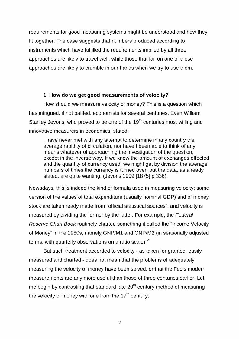
This indeed was the same use that Irving Fisher made of his equation of

exchange MV=PT, but in a much more explicit way that takes us back

immediately to Suppes’ informal example of the mechanical balance. In my

previous examination of Irving Fisher’s use of the analogy of the mechanical

balance for his equation of exchange (see Morgan, 1999), I wrote briefly about

the measurement functions of his mapping of the various numbers he obtained

for the individual elements of the equation of exchange onto a visual

representation of a double-armed balance (see his 1911/1922, fig.17, p 306).11

I suggested that the mechanical balance was not a measuring instrument in

this case, for, like Kemmerer, he measured all the elements on the balance in

separate procedures and both tabled and graphed the series to show how far

the two sides of the equation were equal. Nevertheless, he did use the

mechanical balance visual representation to discuss various measurement

issues: the mapping enabled him to show the main trends in the various series

at a glance and in a way which immediately made clear that the quantity

theory of money could not be “proved” simply by studying the equation of

exchange measurements. He was also prompted by this analogy to solve the

problem of weighted averages by developing index number theory. All this

takes us somewhat away from the point at issue - the measurement of velocity

- but the use of equations of exchange returns again later.

11 See also Harro Maas (2001) on how Jevons used the mechanical balance analogy to bootstrap a measurement of the value of gold and better understand unobservable utility.

12

13

In thinking about all these individual measurement problems, Irving

Fisher took the opportunity to develop not only the fundamentals of measuring

prices by index numbers, but also two neat new ways of measuring the

velocity of money. He regarded his equation of exchange as an identity which

defined the relationships of exchange: it was based on his understanding that

money’s first and foremost function was as a means of transaction. Thus, he

thought it important to measure velocity at the level of individuals: it was

individuals that spent money and made exchanges with others for goods and

services. He developed two new ways to measure velocity.

I will deal with the second innovation first as it can be understood as

working within the same tradition as that used by Petty and Kemmerer, but

instead of simply estimating two number for the two different circulations as

had Petty, or two different circulations of cash and check money as had

Kemmerer, Irving Fisher proposed a more complex accounting in which banks

acted as observation posts in tracing the circulation of payments in and out of

a monetary “reservoir”. This innovation in measuring velocities was introduced

as follows:12

The method is based on the idea that money in circulation and money in banks are not two independent reservoirs, but are constantly flowing from one into the other, and that the entrance and exit of money at banks, being a matter of record, may be made to reveal its circulation outside. .... We falsely picture the circulation of money when we think of it as consisting of a perpetual succession of transfers from person to person. It would then be, as Jevons said, beyond the reach of statistics. But we form a truer picture if we think of banks as the home of money, and the circulation of money as a temporary excursion from that home. If this be true, the circulation of money is not very different from the circulation of checks. Each performs one, or at most, a few transactions outside of the bank, and then returns home to report its circuit. (1909, p 604-5)

He began by dividing all people into three classes: commercial depositors,

other depositors, and non-depositors and thence developed two models to

12 This work was reported in Fisher’s 1909 paper “A Practical Method of Estimating the Velocity of Circulation of Money” and repeated in his 1911 book under the title “General Practical Formula for Calculating V”, Appendix to his Chapter XII, para 4, p 448-460.

14

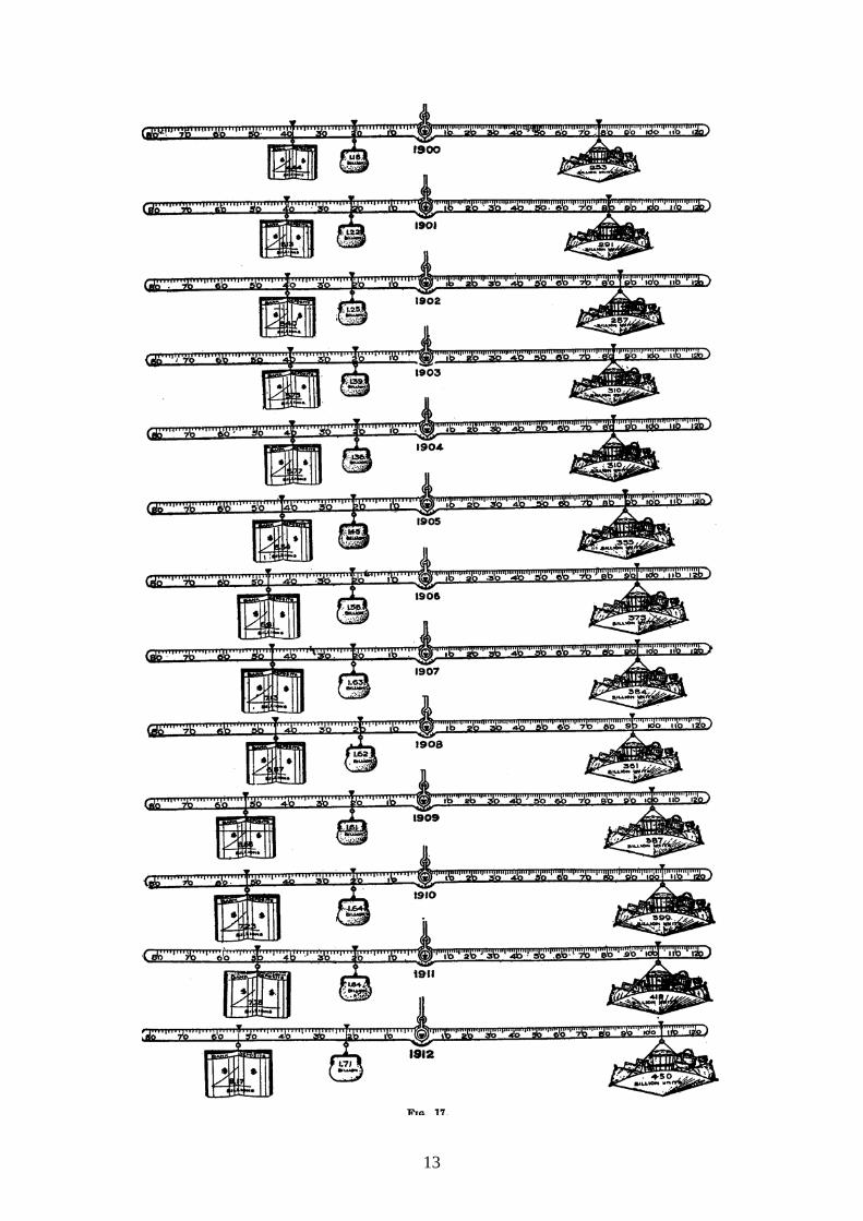
help him map the circulation of money in exchange for goods - first a visual

representation, and, from using that, a second model, an algebraic formula

which allowed him to calculate velocity.

The first visual model (his Figures 18 - reproduced here - and 19, p 453

and 456 of 1911) portrayed the circulation from banks into payment against

goods or services, possibly on to further exchanges, and thence back to

banks. This “cash loop” representation enabled him to define all the relevant

payments that needed to go into his formula and to determine which ones

should be omitted. The relevant payments that he wanted to count for his

calculation of velocity were ones of circulation for exchanges of money against

goods and services, not those into and out of banks, that is, the ones indicated

on the triangle of his diagram, not on the horizontal bars, where B=Banks,

O=Ordinary depositors (salaried men), N=Non-depositors (wage-earners), and

C=Commercial depositors. But banks were his observation posts - they were

the place where payment flows were registered and so the horizontal bars

were the only places where easy counting and so measurement could take

place. Thus his argument and modelling were concerned with classifying all

the relevant payments that he wanted to make measurable and then relating

them, mapping them, in whatever ways possible, to the payments that he

could measure using the banking accounts.13 He used the visual model to

create the mathematical equation for the calculation using the banking

statistics, and this in turn used the flows that were observed (and could be

measured) in order to bootstrap a measurement of the unobservable

payments and thus calculate a velocity of circulation.

13 In doing this, he argued through an extraordinarily detailed array of minor payments to make sure that he had taken account of everything, made allowances for all omissions, and so forth.

15

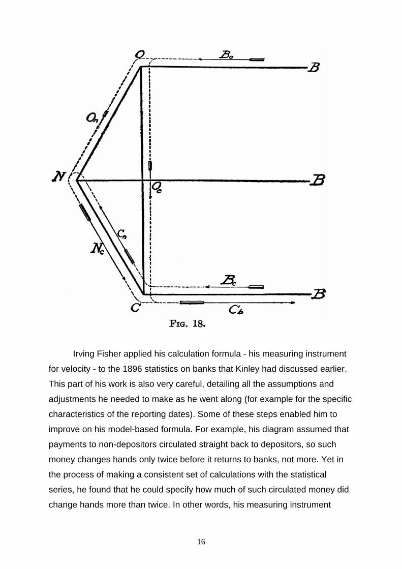
Irving Fisher applied his calculation formula - his measuring instrument

for velocity - to the 1896 statistics on banks that Kinley had discussed earlier.

This part of his work is also very careful, detailing all the assumptions and

adjustments he needed to make as he went along (for example for the specific

characteristics of the reporting dates). Some of these steps enabled him to

improve on his model-based formula. For example, his diagram assumed that

payments to non-depositors circulated straight back to depositors, so such

money changes hands only twice before it returns to banks, not more. Yet in

the process of making a consistent set of calculations with the statistical

series, he found that he could specify how much of such circulated money did

change hands more than twice. In other words, his measuring instrument

16

formula acted not just as a rule to follow in taking the measurement, but as a

tool that allowed him to interrogate the statistics given in the banking accounts

and to improve his measurements.

The velocity measure that Irving Fisher arrived at by taking the ratio of

the total circulation of payments (calculated by his formula) to the amount of

money in circulation for 1896 was 18 times a year (or a turnover time of 20

days). Kinley (1910) immediately followed with a calculation for 1909 based on

Fisher’s formula and showing velocity at 19. Kinley’s calculations paid

considerable attention to how wages and occupations had changed since the

1890 population census, and Fisher in turn responded by quoting directly this

section of Kinley’s paper, and his data, in his The Purchasing Power of Money

(1911). With Kinley’s inputs, and after some further adjustments, Fisher had

two measurements for velocity using this cash loop analysis: 18.6 for 1896

and 21.5 for 1909. The calculation procedure had been quite arduous and

required a lot of judgement about missing elements, plausible limits,

substitutions and so forth. Nevertheless, on the basis of this experience and

the knowledge gained from making these calculations, he felt confident in

claiming that a good estimate of velocity could be made from the “measurable”

parts (rather than the “conjectural” parts) of his formula (p 475, 1911), that is,

he used the following measuring instrument equation (referring to his cash-

loop diagram):

MV= Oc + On + Cn + Nc = bank deposits (Oc+Nc) + wages (On+Cn)

He concluded that “money deposits plus wages, divided by money in

circulation, will always afford a good barometer of the velocity of circulation.”

(1911, p 476) . It is perhaps surprising that he did not use this modified

measuring instrument, his “barometer”, to calculate the figures for velocity

between 1897-1908! Rather, the two end points acted as a calibration for

interpolation. Nevertheless, the way that he expressed this shows that his

cash loop model and subsequent measurement formula can be classified as a

17

sophisticated version of Petty’s tradition of using the class of payers and

payments to determine the velocity measurement.

The other (chronologically earlier) new way of measuring velocity

introduced by Irving Fisher was an experimental sample survey that he

undertook himself and reported briefly in 1897. (A fuller report of this survey

was included in his 1911 book.) In his 1897 paper, he wrote of the possibility

of taking a direct measurement of velocity:

... just as an index number of prices can be approximately computed by a judicious selection of articles to be averaged, so the velocity of circulation of money may be approximately computed by a judicious selection of persons. Inquiry among workmen, mechanics, professional men, &c., according to the methods of Le Play might elicit data on which useful calculations could be based, after taking into account the distribution of population according to occupations. (p 520).

Again, this has shades of Petty’s approach, a groups of spenders whose

varied transactions behaviour are the key to understanding the overall

transactions velocity.

Fisher began this task by enlisting the help of Yale students. After an

initial disappointing survey, in which he asked respondents for annual amounts

of expenditure and cash balances (and which he supposed that they merely

guessed), he then asked for volunteers to undertake a more systematic

survey. He asked them to keep records of their cash expenditure and cash

balances each day for a month as a way to get some reasonably accurate

statistics on velocity or turnover of money in exchange for goods and services.

He gained 116 good quality responses, of which 113 were students. These

data provided him with an average velocity (money spent during the month

divided by average cash balance in their pocket) of 66. The returns enabled

him to divide the total sample into sub-samples according to total expenditure,

and so to calculate associated velocities, showing a rising scale of velocities

from 17 (for the lowest category of total expenditure) to 137 (for the highest).

The average stock of money in the pocket overnight rose with the day’s

average expenditure, but fell as a proportion of that expenditure. These

investigations fed into his discussions about the determinants of velocity - and

18

what made it change, and about what effects changes in velocity had on other

entities in the equation of exchange.14

In this period of work, attempts to measure velocity take it for granted

that velocity has to be measured as far as possible directly - either by sample

survey, or by figuring out circulations of money - or indirectly by trying to get at

velocity measures through other payment measurements or even by plausible

guess work with them. Though the equations of exchange come in, they are

regarded as calculation checking devices rather than measuring instruments in

their own right. With Irving Fisher, we see two new kinds of measuring

instruments being developed to apply to the problem of measuring velocity,

one based on a sampling strategy, the other on a representational model.

Neither of these instruments seems to have turned into the kind of

standardized quantitative rules - to use Porter’s terminology - that betoken well

accepted measuring instruments, although as we shall see, there have been

later uses of the cash-loop model, and there have been later sample survey

investigations.

3.2 Interlude on Concepts

Concepts form one of the important elements in measuring instruments.

It is often held that we need a theory of what governs the behaviour of an

entity before we can measure it. This seems to require too much. First, there

are good examples in measurement history where reliable measuring

instruments have been constructed on theories which turn out later to be

wrong - eg thermometers.15 Second, the history of economic measurement

suggests that conceptual material is required, but not necessarily a causal

account or theory of the behavioural variations in the element being measured.

For example, we need a clear concept of the difference between the cost of

living and the standard of living to determine relevant index number measuring 14 See Chapter VIII of Fisher 1911, to which the report of the Yale experiment forms an Appendix, pp379-382.

19

formulae, but we don’t have to commit to the causes of changes in the cost of

living to determine the relevant measuring formula.

In this context, Holtrop’s 1929 discussion of early theories of the velocity

of circulation, makes an interesting distinction between two concepts of

velocity. One, held by Petty (and by Cantillon), understands the idea of

velocity as a circular course in which we measure the time taken by money to

travel around the circle of payments: ie the relation between circulation

distance and time - a “motion-theory” concept. Holtrop’s expression of his

insight is striking: “The partisans of the motion theory are more or less inclined

to regard the velocity of circulation as a property of money, as a kind of energy

which is inherent to it. ... If, however, the velocity is a property of money, then

the supply of money is not a singular but a compound magnitude, being

constituted of the product of quantity and velocity.” (1929, p 522.) In contrast,

according to Holtrop, we also find in early work, the concept of a “cash-

balance theory” or the total need of money as in a position of rest in the

economy - to which the velocity of circulation is inversely proportional (a

position he attributes to Locke). Holtrop suggests we understand this concept

as a focus on the demand side of money in which “the size of cash balances is

[dependent] .... on the will of the owner, which is governed by economic

motives.” (1929, p 523.)

In looking at these earlier methods of taking measurements of velocity

(rather than theorizing about it), we can see that they rely on concepts of

velocity, but the positions do not seem to map onto Holtrop’s account. We saw

a “need of money” argument made by Petty, not for cash balances or money

at rest, but as an amount of money needed for circulation - ie Holtrop’s motion-

theory concept. Irving Fisher’s ideas are also difficult to characterize. Holtrop

(p 522) argues that Fisher had a cash-balance concept of velocity, but I find

this doubtful for his methods of measuring velocity were essentially designed

to measure the money flow. Although his sample survey method appears to be

measuring the cash balance, Fisher’s idea was to measure the cash as it went

15 See Chang’s 2004 book on the history of measuring heat.

20

through his student subjects’ pockets each day, just as, in his cash loop

method, he used the point of payments into and out of a position of rest as a

way to get at the payment flows themselves. His idea of money velocity can be

well characterized by Holtrop’s idea of an “energy” or compound property of

money, somehow inseparable from its quantity.

Open disagreement about conceptual issues in discussions of velocity

in the late nineteenth century continued into the interwar period. The masterly

treatment of these arguments by Arthur Marget (1938) in the context of the

theory of prices provides an exhaustive analysis of theorizing about velocity.

But Marget’s analysis and critique could not stem the tide; in place of the

earlier “transactions velocity” (the number of times money changes hands for

transactions during a certain period and the concept that we have found in the

examples of measurement from Petty to Irving Fisher), velocity was re-

conceived as “income velocity”: the number of times the circular flow of

income went around during the period. Although the velocity measures of the

later 20th century are based on thinking about the individuals’ demand for

money in relation to their income, and might even be considered a cash-

balance approach, this “hybrid” concept of velocity came to be “expressed” as

the ratio of national income to money in circulation. As we shall see, the issue

of compound properties comes back to strike those grappling with the problem

of uncertainty and variability in these measurements of monetary aggregates

at the U.S. Federal Reserve Board.

3.3 Indirect Measurement of Income Velocity

Economists considering questions about velocity in the latter half of the

20th century have tended to stick with this income notion of velocity, not only in

discussion, but also in measurement. Yet their measurements are far from

providing numbers that fit the concept of the individual’s demand for money

implied by Holtrop or understood by the early Cambridge School. Rather,

since 1933, measurements have been made on the basis of aggregates, far

21

from the conceptual requirements of individual demand.

Michael Bordo’s elegant New Palgrave piece on Equations of Exchange

(1987), discussed how equations of aggregate exchange, considered as

identities, have been important in providing building blocks for quantity

theories and causal macro-relations. Not only for theory building, for, as we

have seen, equations of exchange provided resources for measuring the

properties of money. In the work of Kemmerer and Fisher, their equation of

exchange, the identity MV=PT, provided a checking system for their

independent measurements of transactions circulation and so velocity. In the

more recent history of velocity, the income equation of exchange, namely

M=PY/V, has formed the basis for measuring instruments that enable the

economist to measure velocity indirectly without going through the complicated

and serious work of direct measurement done by Fisher and Kemmerer.

This income equation of exchange, rearranged to provide: V=PY/M

(velocity = nominal income divided by the money stock), became a generic

measuring instrument for velocity in the mid 20th century, generic in the sense

that different money stock definitions provide different associated velocities,

and different income definitions and categories alter the measurements of

velocity made. For example, Richard Selden’s 1956 paper on measuring

velocity in the US reports 38 different series of “estimates” for velocity made

by economists between 1933 and 1951 and adds 5 more himself. They use

various versions of aggregate income as the numerator (personal, national

income, even GDP) and various versions of M as the denominator. These are

called “estimates” both because the measurers could not yet simply take their

series for national income (or equivalent) and money stock ready made from

some official source (national income figures were only just being developed

during this time), and because many of the measurers, as Selden, wished to

account for the behaviour of velocity. They wished to see if it exhibited long-

term secular changes, so understood themselves to be estimating some kind

of velocity function to capture the changing level of velocity as the economy

developed. Like the late nineteenth century measurers whose work we have

22

considered already, there was considerable variation in the outcome

measurements.

Boumans (2005) has placed considerable emphasis on variation and

invariance in measurement. It is useful to think about that question here.

Clearly, we want our measuring instrument to be such that it could be used

reliable over periods of time, and could be applied to any country for which

there are relevant data, to provide comparable (ie standardized)

measurements of velocity. At the same time, we want our measuring

instrument to capture variations accurately, either between places or over

time. In the context of this measuring instrument, clearly if the ratio were

absolutely constant, velocity would also be unvarying, so that the formula

would not be needed once we had found the constant, something like a

natural constant perhaps. If velocity is not a natural constant, does the formula

work well as a measuring instrument - like for example a thermometer - to

capture that variation? From the formula, V=PY/M, we can see that variation in

both the numerator and denominator may cause alterations in the

measurements for V. It appears to operate as a measuring instrument

capturing variations in velocity, but in fact these variations are reflections of

changes in one or other of the money supply or nominal income. How are we

to interpret the velocity that we measure in this way? And what are the

sources of velocity’s independent freedom for variation when the equation

V=PY/M is used as a measuring instrument?

One economist who, without using this language of measuring

instruments, has taken an interpretation close to denying velocity any

independence or autonomous variation is Benjamin Friedman (1986). He, for

the most part, keeps “velocity” in quotes, partly to remind us that the velocity

measured with nominal income is not a true velocity in the sense of the

transactions velocity of the older measurement, but partly as well to point to its

lack of independent conceptual content:

.... it is useful to point out the absence of any economic meaning of “velocity” as so defined - other than, by definition, the income-to-money ratio. Because the “velocity” label may seem to connote deposit or

23

currency turnover rates, there is often a tendency to infer that “velocity” defined in this way does in fact correspond to some physical aspect of economic behavior. When the numerator of the ratio is income rather than transactions or bank debits, however, “velocity” is simply a numerical ratio. ... The issue of money or credit movements versus their respective “velocities”, in a business cycle context, is just the distinction between movements of nominal income that match movements of money or credit and movements of income that do not, and hence that imply movements in the income-to-money or income-to-credit ratio. (Friedman, 1986, p 411-2.)

If we observe variations in the numbers produced for such “velocity”, it alerts

us to changes in the nominal income that are not due to increases in the

money (or credit) supply. It offers a way to decompose changes in nominal

income across different business cycles, but it is not something that can

represent independent variation in velocity: “Saying that money growth

outpaced income growth because velocity declined is like saying that the sun

rose because it was morning.” (Friedman, 1988, p 58.) Friedman is effectively

denying an autonomous or independent status to such a velocity: the equation

operates to produce numbers, and these are taken as an indicator for

something else, but in terms of the representational theory, there is no entity -

no independent well-conceptualized thing called velocity - there to be

measured.

In the 1980s, the Governors of the Federal Reserve Board also

grappled with the problem of what velocity is when measured by such an

equation. For example, the transcript of the Federal Open Market Committee

Meeting (FOMC) Meeting for July 6-7th of 1981 finds its members arguing

over which version of M1 to target (M1, M-1A or M-1B). The level of

uncertainty in setting the target ranges for money supply growth was high, and

it was an uncertainty that came from several sources. First there was the

normal problem of predicting the economic future of the real economy and the

monetary side of the economy in relation to that. Secondly, and equally

problematic, seemed to be the uncertainty associated with the difficulty of

locating a reliable measure of money supply when the stable trend in its

24

growth broke down in the early 1980s. This may have been to do with

institutional changes and people reacting by “blurring” distinction between

transactions and savings balances. As Chairman Volcker expressed it is “not

that we know any of these things empirically or logically” (p 81).

The difficulties of locating a money supply definition that provides

stability in measuring the relevant concept of money was matched in - and

indeed, intimately associated with - the problem of velocity measurement.16

The target ranges discussed in the committee were understood to be

dependent on both what happened to a money stock that was unstable and a

velocity that was subject to change. The instability of the money stock

measurements were understood to be not only normal variation as interest

rates changed, but also more unpredictable changes in behaviour because of

innovations in the services offered to savers.17 Those factors in turn were

likely to affect the velocity of money, if conceived as an independent entity.

Here though, the situation is further confused by the fact that, as the

Governors were all aware, the velocity numbers that they were discussing

were not defined nor measured as independent concepts, but only by their

measurement equation - namely as the result of nominal income divided by a

relevant money supply. Thus, variations in velocity were infected by the same

two different kinds of reasons for variations as the money supply. Velocity was

as problematic as the money stock. The difficulties are nicely expressed in this

contribution from Governor Wallich:

We seem to assume that growth in velocity is a special event due to definable changes in technology. But if people are circumventing the need for transactions balances right and left by using money market funds and overnight arrangements and so forth, then really all that is happening is that M-1B is becoming a smaller part of the transactions balances. And its velocity isn’t really a meaningful figure; its just a statistical number relating M-1B to GNP. But it doesn’t exert any

16 For background to the troubles the Fed had in setting policy in this period, see Friedman, (1988). 17 This may be interpreted as Goodhart’s Law, that any money stock taken as the object of central bank targeting will inevitably lose its reliability as a target. However, the reasons for the difficulty here were not necessarily financial institutions finding their way around constraints but the combination of expected savings behaviour in response to interest rates and unexpected behaviour by savers in response to new financial instruments.

25

constraints. That is what I fear may be happening, although one can’t be very sure. But that makes a rise in velocity more probable than thinking of it in terms of a special innovation. (FOMC transcript, July 1981, p 88.)

Because of these causes of variations in the money supply, velocity variations

also appeared unpredictable. Either velocity was a meaningful concept, but is

variations were unpredictable, and so it provided no anchor or constraints; or it

was merely the ratio of GDP to M-1B, and so provided no independent anchor

or constraint. Either way, it was no help in the problem of predicting the future

range of money supply and so targeting.

These knotty problems experienced in the early 1980s are neatly

dissected in a presentation on velocity to the October 1983 meeting of the

FOMC by Stephen H. Axilrod from the Fed staff:

Velocity is of course the link between money and GNP in the equation of exchange (MV=PY), but whether its behavioral properties are sufficiently stable or predictable to provide a strong basis for monetary targeting as a means of attaining ultimate economic objectives over time has, as we all know, been a continuing subject of intensive economic debate. At one extreme, velocity might be considered as no more than the arithmetic by-produce of forces acting independently on the supply of money and other forces acting independently on GNP - hence, an economically meaningless number and making the whole equation of exchange useless as a policy framework. At the other extreme velocity might be found to have a trend all of its own - hence providing a reasonably predictable link between money and GNP, and giving policy content to the equation of exchange.

From another viewpoint, velocity can be considered as the inverse of the demand for money relative to GNP. If we can know what influences the demand for money - and among the factors explaining money demand are income, transactions needs, interest rates, wealth and institutional change - then we can predict the money needed, for, say, a given GNP. But the more one has to go beyond income or transactions needs in explaining money demand, the weaker is the argument for pure or rigid monetary targeting. (Axilrod, 1983 p 1)

So, measured velocity has three faces. On one side, it is simply the measured

ratio between two things, each of which are determined elsewhere than the

equation of exchange: because velocity has no autonomous causal

connections, it provides for no measure of V that can be used for policy

26

setting. On the second, it exhibits its own (autonomous) trend growth rate

(sometimes unreliably so) which could be useful for prediction and so policy

setting for the two elements from which it is measured. On the third, it has a

relationship to the behaviour of money demand, a relationship which is both

potentially reliable and potentially analysable, so that it could be useful for

understanding the economy and for policy work, but here the focus seems to

have reversed itself: understanding the determinants of velocity now seems to

be the device to understand the behaviour of the money stock, even while the

measuring instrument works in the opposite direction.

Standing back and using our ideas on measuring instruments, it seems

clear that the problem in the early 1980s was not so much that the instrument

was just unreliable in these particular circumstances, but that the instrument

itself has design flaws. In taking the formula V=nominalGDP/money stock as a

measuring instrument that is reliable for measuring velocity, there is a certain

assumption of stability within the elements that make up the measuring

instrument and within their relationships. If the dividing line between velocity

and money supply is not strict, the latter cannot be used as a reliable

component in a measuring device intended for the former. It is rather like using

a thermometer where the glass tube and the mercury column keep dissolving

into each other. There are two senses in which this problem might be

understood in the velocity case. First the changes in behaviour of people and

in categorization of elements mean that there is a switching between what

counts as the money quantity and what counts as the velocity category. This

seems to be a generic problem in this field of economics, for as Tom

Humphrey has so astutely remarked in his history of the origins of velocity

functions, “one era’s velocity determinants become another’s money-stock

components.” (Humphrey, 1993, p 2.) The second is, as Holtrop characterised

it - we may really have a compound property, and so, despite the

measurement formula, velocity can not be separated out from the money

stock. In terms of Porter’s trust in numbers, we have a standard quantitative

rule to measure velocity, one supported by a well-respected bureaucracy and

27

vast amounts of data collection and manipulation, but the measuring device

lacks certain characteristics which make us believe that its numbers are

trustworthy. It lacks the requirements of invariance specified by Boumans for

measuring instruments because the device does not capture the independent

variations in the thing being measured. It fails also in Suppes’ representational

theory of measurement in that the mapping between empirical and numerical

structures seems not to be operational.

3.4 Regression Measures of Velocity

These 2nd and 3rd faces we find mentioned by Axilrod are ones that

many economists have taken up when they assume that velocity does indeed

have its own behaviour. Arguments over what determines the behaviour of

velocity and whether it declines or rises with commercialization were a feature

of our late 19th and early 20th century measurers. They can be seen as

following suggestions made by many earlier economists (mostly non-

measurers) who discussed both the economic reasons (such as changes in

income and wealth) as well as the institutional reasons (in changes in level of

monetization or in financial habits) for velocity to change over time.18

In the twentieth century, economists have assumed that velocity can be

investigated just like any other entity through an examination of the patterns

made by its measurements. Some, like Selden (1956) have used correlations

and regressions to try to fix the determinants of variations in velocity.

Particular attention was paid to the role of interest rates in altering people’s

demand for money and so velocity. Selden himself reported regressions using

bond yields, wholesale prices and yields on common stocks to explain the

behaviour of velocity (though without huge success). More recently and

notably, Michael Bordo with Lars Jonung (1981 and 1990), have completed a

considerable empirical investigation into the long run behaviour of velocity

18 Excellent accounts of economists’ attempts to explain velocity behaviour can be found in Humphrey, 1993 and of these institutional changes can be found in Friedman, 1986.

28

measurements using regression equations to fix the causes of these

behaviours statistically and thence to offer economic explanations for the

changes implied in the velocity measurements. Others have argued that there

is no economically interesting behavioural determinant, that velocity follows a

random walk and can be characterised so statistically (for example Gould and

Nelson, 1974).

The use of regression equations in the context of explaining the

behaviour of velocity is but one step removed from using regression equations

as a measuring instrument to measure velocity itself. Regression forms a

different kind of measuring instrument from those of direct concept based

measurement used from Petty to Irving Fisher and from the indirect

measurement using equations of exchanges (such as those surveyed by

Seldon or in the Fed’s formulae). The principles of regression depend on the

statistical framework and theories which underlay all regression work. An

additional principle here is that by tracing the causes which make an entity

change, we can track the changes in the entity itself. Alfred Marshall

suggested this as one of the few means to get at velocity behaviour: “The only

practicable method of ascertaining approximately what these changes are is to

investigate to what causes they are due and then to watch the causes.”

(Marshall, 1867-74, 1975, p 170.) Marshall did not of course use regression for

this, but his point is relevant here: regression forms a measuring instrument

not only for tracing these changes but for measuring them - and so velocity -

too.

One option has been to use regression to measure or “estimate” velocity

by using the opportunity cost of holding money as the estimator (see for

example, Orphanides and Porter, 1998). The velocity concept they measured

here is an entirely different one from the directly observable entity of the kind

supposed or measured by Fisher. By constitution, it is an idealized entity

named the “equilibrium velocity”. This may be well-defined conceptually, but it

is a different concept altogether from those sought and measured in earlier

times.

29

Another example combines the regression measuring instrument with

that of Fisher’s transactions loop model. Mars Cramer (1986) set out to

measure the transactions velocity for the US in the post-war period. He began

with Fisher’s cash loop idea to get at measures of currency velocity, and then

developed the equation of exchange into a form which included a parameter

for “hypothetical pure transactions velocity”. This parameter was measured

using regression and then plugged back into his equation of exchange to

provide the series of measurements of velocity over the period showing a rise

in the transaction velocity of demand deposits. Clearly, Mars Cramer rivals

Irving Fisher’s inspired ingenuity as a measurer. And he brings us back almost

to where we started, but not quite, for he too is now purporting to measure a

different concept - an idealized version of the transactions velocity.

Conclusion: Measurements that Travel Well It is easy to put a number to the “velocity of money” using an indirect

calculation via the equation of exchange V=PY/M, but a difficult thing to

measure with any confidence using that standard method. The standardized

quantitative rules this measuring instrument entails do not seem to provide

numbers that adequately represent the property we are trying to measure

even though the data fed in come from trustworthy sources. The model seems

to act as a measuring instrument, yet does not have the reliability we require in

such instruments. We can understand this equation of exchange as a

numerical relational structure, but it is not quite clear that it is an empirical

relational structure. In past times, when the monetary economy was rather

stable, the numbers it produced were considered reliable and travelled well.

When times proved unstable, it became clear that this was a case of feeding

trustworthy data into an untrustworthy measuring instrument: the velocity of

money numbers it produced could not be used as “hard facts” upon which

action could be based.

We have also seen that earlier economists tried to secure trustworthy

30

measurements of velocity using a variety of other kinds of measuring

instruments: sample surveys, direct calculation, and so forth. These often

relied on feeding in guesstimated data, of rather poor quality compared to

modern data. Consequently, the numbers generated in these earlier times

have not travelled well into the present. Yet these earlier measuring

instruments were rather better designed to create good measurements. Even

though these instruments have their individual problems, their design treats

velocity as a separate, conceptually well defined, entity, and so the

measurements they produce might well be more sustainable and so

trustworthy.

31

Works Cited

Axilrod, Stephen H. (1983) “Velocity Presentation for October FOMC Meeting”

online at 18 August 2006 at

http://www.federalreserve.gov/FOMC/transcripts/1983/831004StaffState.pdf

Banzhaf, Spencer (2001) “Quantifying the Qualitative: Quality-Adjusted Price

Indexes in the United States, 1915-61" in Klein and Morgan, 2001, pp

345-370.

Board of Governors of the Federal Reserve System (1984, 1986) Federal

Reserve Chart Book

Bordo, Michael D. (1987) “Equations of Exchange” in J. Eatwell, M. Milgate

and P. Newman The New Palgrave: A Dictionary of Economics Vol 2

(London: Macmillan) pp 175-177.

Bordo, Michael D. and Lars Jonung (1981) “The Long-Run Behavior of the

Income Velocity of Money in Five Advanced Countries, 1870-1975: An

Institutional Approach” Economic Inquiry 19:1, 96-116.

Bordo, Michael D. and Lars Jonung (1990) “The Long-Run Behavior of

Velocity: The Institutional Approach Revisited” Journal of Policy

Modeling 12:2, 165-97.

Boumans, Marcel (1999) “Representation and Stability in Testing and

Measuring Rational Expectations” Journal of Economic Methodology,

6:3, 381-401.

Boumans, Marcel (2001) “Fisher’s Instrumental Approach to Index Numbers”

in Klein and Morgan, 2001, 313-344.

Boumans, Marcel (2005) How Economists Model the World to Numbers

(London: Routledge).

Chang, Hasok (2004) Inventing Temperature: Measurement and Scientific

Progress (Oxford: Oxford University Press).

Chao, Hsiang-Ke (2002 and forthcoming) Representation and Structure: The

Methodology of Economic Models of Consumption (University of

Amsterdam thesis, forthcoming, Routledge).

32

Cramer, J.S. (Mars) (1986) “The Volume of Transactions and the Circulation of

Money in the United States, 1950-1979" Journal of Business &Economic

Statistics 4:2, 225-232.

Federal Open Market Committee (1981) Transcripts of July 6-7 Meeting at

http://www.federalreserve.gov/FOMC/transcripts/1981/810707Meeting.pdf

(online at 18 August 2006)

Finkelstein, Ludwik (1974) “Fundamental Concepts of Measurement: Definition

and Scales” Measurement and Control, 8: 105-111 (Transaction Paper

3.75.)

Finkelstein, Ludwik (1982) “Theory and Philosophy of Measurement” in

Handbook of Measurement Science, Vol 1: Theoretical Fundamentals

ed P.H. Sydenham (New York: Wiley) Chapter 1.

Fisher, Irving (1897) “The Role of Capital in Economic Theory”, Economic

Journal 7, 511-37.

Fisher, Irving (1909) “A Practical Method of Estimating the Velocity of

Circulation of Money”, Journal of the Royal Statistical Society, 72:3,

604-618.

Fisher, Irving (1911/1922) The Purchasing Power of Money (New York:

Macmillan).

Fisher, Willard (1895) “Money and Credit Paper in the Modern Market”,

Journal of Political Economy, 3:4, 391-413.

Friedman, Benjamin M. (1986) “Money, Credit, and Interest Rates in the

Business Cycle” in Robert J. Gordon ed: The American Business Cycle,

NBER Studies in Business Cycles, Vol 25 (Chicago: University of

Chicago Press), pp 395-458.

Friedman, Benjamin M. (1988) “Lessons on Monetary Policy from the 1980s”

Journal of Economic Perspectives, 2:3, 51-72.

Gould, John P. and Charles R. Nelson (1974) “The Stochastic Structure of the

Velocity of Money” American Economic Review 64:3, 405-418.

Holtrop, M.W. (1929) “Theories of the Velocity of Circulation of Money in

Earlier Economic Literature” Economic Journal Supplement: Economic

33

History 4: 503-524.

Humphrey, Thomas M. (1993) The Origins of Velocity Functions” Economic

Quarterly, 79:4, 1-17.

Jevons, William.St (1909) [1875] Money and the Mechanism of Exchange

(London: Kegan Paul, Trench, Trübner & Co.).

Kemmerer, Edwin W. (1909) Money and Credit Instruments in their Relation to

General Prices 2nd edn. (New York: Henry Hold & Co.).

Kinley, David (1897) “Credit Instruments in Business Transactions” Journal of

Political Economy, 5:2, 157-74.

Kinley, David (1910) “Professor Fisher’s Formula for Estimating the Velocity of

the Circulation of Money”, Publications of the American Statistical

Association, 12, 28-35.

Klein, Judy and Mary S. Morgan (2001) The Age of Economic Measurement

Annual Supplement to Volume 33, History of Political Economy

(Durham: Duke University Press).

Krantz, D.H., R.D. Luce, P. Suppes and A. Tversky (1971) Foundations of

Measurement, Vol 1 (New York: Academic Press).

Maas, Harro (2001) “An Instrument Can Make a Science: Jevons’s Balancing

Acts in Economics” in Klein and Morgan, 2001, 277-302.

Marget, Arthur W. (1938) The Theory of Prices, Vol I (New York, Prentice Hall)

Marshall, Alfred (1975) The Early Economic Writings of Alfred Marshall, Vol 1

Ed J.K. Whitaker, Macmillan for the Royal Economic Society.

Mitchell, Wesley C. (1896) “The Quantity Theory of the value of Money”

Journal of Political Economy, 4:2, 139-65.

Morgan, Mary S. (1999) “Learning from Models” in Morgan, Mary S. and

Margaret Morrison, Models as Mediators: Perspectives on Natural and

Social Science (Cambridge: Cambridge University Press), pp 347-88.

Morgan, Mary S. (2001) “Making Measuring Instruments” in Klein and Morgan,

2001, pp 235-251.

Morgan, Mary S. (2003) “Business Cycles: Representation and Measurement”

in Monographs of Official Statistics: Papers and Proceedings of the

34

Colloquium on the History of Business-Cycle Analysis ed D.Ladiray

(Luxemboug: Office for Official Publications of the European

Communities), pp 175-183.

Orphanides, Athanasios and Richard Porter (1998) “P* Revisited: Money-

Based Inflation Forecasts with a Changing Equilibrium Velocity*”

Working paper, Board of Governors of the Federal Reserve System,

Washington DC.

Petty, William (1997) [1899] The Economic Writings of Sir William Petty Vol I

(1899, Cambridge: Cambridge University Press; reprinted Routledge:

Thoemmes Press, 1997).

Porter, Theodore M. (1994) “Making Things Quantitative” in Accounting and

Science: Natural Enquiry and Commercial Reason ed: Michael Power

(Cambridge: Cambridge University Press), pp 36-56.

Porter, Theodore M. (1995) Trust in Numbers: The Pursuit of Objectivity in

Science and Public Life (Princeton: Princeton University Press).

Rodenburg, Peter (2006) The Construction of Measuring Instruments of

Unemployment (University of Amsterdam thesis).

Selden, Richard T (1956) “Monetary Velocity in the United States” in Studies in

the Quantity Theory of Money ed M. Friedman (Chicago: University of

Chicago Press), pp 179-257

Suppes, Patrick (1998) “Measurement, Theory of” in E. Craig, Ed, Routledge

Encyclopedia of Philosophy, London, Routledge. Retrieved October 27,

2004, online at 18 August 2006 at:

http://www.rep.routledge.com/article/Q066?ssid=388873355&n=8#

Suppes, Patrick (2002) Representation and Invariance of Scientific Structures

(Stanford: CSLI).

Sydenham, P.H. (1982) “Measurements, Models, and Systems” in Handbook

of Measurement Science, Vol 1: Theoretical Fundamentals ed P.H.

Sydenham (New York: Wiley) Chapter 2.

35

LONDON SCHOOL OF ECONOMICS DEPARTMENT OF ECONOMIC HISTORY WORKING PAPERS IN: THE NATURE OF EVIDENCE: HOW WELL DO “FACTS” TRAVEL? For further copies of this, and to see other titles in the department’s group of working paper series, visit our website at: http://www.lse.ac.uk/collections/economichistory/ 2005 01/05: Transferring Technical Knowledge and innovating in Europe, c.1200-c.1800

Stephan R. Epstein 02/05: A Dreadful Heritage: Interpreting Epidemic Disease at Eyam, 1666-2000

Patrick Wallis 03/05: Experimental Farming and Ricardo’s Political Arithmetic of Distribution

Mary S. Morgan 04/05: Moral Facts and Scientific Fiction: 19th Century Theological Reactions to Darwinism in Germany

Bernhard Kleeberg 05/05: Interdisciplinarity “In the Making”: Modelling Infectious Diseases Erika Mattila 06/05: Market Disciplines in Victorian Britain Paul Johnson 2006 07/06: Wormy Logic: Model Organisms as Case-based Reasoning Rachel A. Ankeny

08/06: How The Mind Worked: Some Obstacles And Developments In The Popularisation of Psychology Jon Adams 09/06: Mapping Poverty in Agar Town: Economic Conditions Prior to the Development of St. Pancras Station in 1866 Steven P. Swenson 10/06: “A Thing Ridiculous”? Chemical Medicines and the Prolongation of Human Life in Seventeenth-Century England David Boyd Haycock 11/06: Institutional Facts and Standardisation: The Case of Measurements in the London Coal Trade. Aashish Velkar 12/06: Confronting the Stigma of Perfection: Genetic Demography, Diversity and the Quest for a Democratic Eugenics in the Post-war United States Edmund Ramsden 13/06: Measuring Instruments in Economics and the Velocity of Money Mary S. Morgan