measuring regional inequality: a comparison of coefficient of variation … · 2016-11-22 ·...

The Open Geography Journal, 2009, 2, 25-34 25

1874-9232/09 2009 Bentham Open

Open Access

Measuring Regional Inequality: A Comparison of Coefficient of Variation and Hoover Concentration Index

Yefang Huang* and Yee Leung

Department of Geography and Resource Management, The Chinese University of Hong Kong, Shatin, N.T., Hong Kong

Abstract: Many measures, particularly the coefficient of variation (CV) and Hoover concentration index (CI), have been

used in the study of regional inequality. However, opposite results are often obtained from different quantitative measures

which are supposedly showing the same pattern of regional inequality. This paper employs Jiangsu province in P.R. China

as a case study to explain how two measures, CV and CI, can produce completely contrasting results. This has been

achieved by explicating the original CV and CI, and by appropriately modifying these indices. Two major reasons leading

to different trends exhibited by the CV and CI for the same data set have been identified. They are the population weights

attached to areal units and the absolute deviation from the mean in the original data. The findings serve as a note of

caution on the employment of measures to unravel regional inequality. Inappropriate use of indices might lead to invalid

conclusion about differential in regional development.

Keywords: Coefficient of variation, Hoover concentration index, regional development, Jiangsu province, inequality.

INTRODUCTION

There has been a growing interest in regional economics and geography on the long-term convergence in per capita income between sub-national regions and countries. China, for example, has experienced rapid economic growth since the implementation of the reform and open door policy in 1978. Regional inequalities within a region or between regions, on the other hand, have been significant phenomena causing serious concern. To gain a further understanding of this coexistence, a number of studies have been carried out on regional economic growth and regional inequality in China [1, 2]. Apparently, the widening or narrowing of regional inequality in China in the Mao and post-Mao periods has been a subject of debate [3-5]. While some researchers believed that regional inequality was narrowed in the period of Mao’s even-development strategy [6, 7], others argued the opposite [8-10]. Similarly, there are also different judgments about regional inequality in post-Mao period although uneven regional development strategies have been adopted [11-14].

How have such contrasting conclusions been reached is an interesting issue. It is also important to identify the reasons causing such contrasting conclusions. There are many reasons which may lead to the divergent views on the trends of spatial inequality in China, such as the use of different spatial scales, economic indicators, quantitative measures, and time periods [15-18]. To substantiate one’s claim on regional inequality, the use of some kinds of quantitative measures is inevitable. Interesting enough, opposite results are often obtained from different

*Address correspondence to this author at the Department of Geography and

Resource Management, The Chinese University of Hong Kong, Shatin,

N.T., Hong Kong; Tel: 852-2609-6596; Fax: 852-2603-5006;

E-mail: [email protected]

quantitative measures which, however, are meant to be consistent in their deliveries. Even though many people have noticed the contradicted results [19], the paper has definitely revealed the reasons by quantified decomposition. The purpose of this paper is to investigate how two measures with the same intention can produce completely contrasting results in the study of regional inequality in Jiangsu province, P.R. China. It serves as a note of caution on the employment of measures to unravel regional inequality, contributing to more accurate analyses and understanding of on regional inequality.

Over the years, many measures have been used in the study of regional economic inequality, such as the coefficient of variation (CV), Hoover concentration index (CI), standardized difference (STD Dif), Theil’s regional inequality index or generalized entropy (GE), Gini coefficient, Lorenz curve and location quotients (LQ). Different trends may be revealed using different measures in the study of regional inequality [20]. Tsui, for example, examined the trends of interprovincial inequality in the post-1978 reform era in China using different inequality measures of CV, Gini coefficient and GE [11]. The trends of interprovincial inequalities were consistent, but the magnitudes of change over time were different. In another study, Zhao analyzed the spatial disparities of economic development in China between 1953 and 1992 using measures of CV and STD Dif for per capita national income and the growth rate of national income [16]. He found that the trends of interregional inequality and interprovincial inequality in terms of CV and STD Dif were quite different over the study period.

Intrigued by these empirical results and recent opposite results produced by the coefficient of variation (CV) and concentration index (CI), we attempt to use CV and CI (whose relationship can be explicitly analyzed) as a basis of this study to find out the reasons leading to contrasting

26 The Open Geography Journal, 2009, Volume 2 Huang and Leung

results which are not supposed to happen. For substantiation, Jiangsu province in P. R. China is employed as a case study. Even though CV and CI have been developed for a quite long time, they are still important measures for regional studies and Geography. On the other hand, why only these two methods have been chosen is that they are relatively straightforward to decompose their formulae to review their difference. It is much difficult to link Gini coefficient with CV and CI, which maybe the reason that Roger and Sweeney (1998) has only addressed dramatic visual difference between the Gini and the CV index plots in measuring the spatial focus of origin-destination-specific migration flows [21].

We outline the extents and trends of regional inequality in Jiangsu as measured by CV and CI in next section. Then, we propose several suitably modified indices to identify the causes of different trends exhibited by CV and CI. The paper is summarized with some concluding remarks in last section.

SPATIAL INEQUALITY OF REGIONAL DEVELOP-

MENT IN JIANGSU PROVINCE

Background of Jiangsu Province

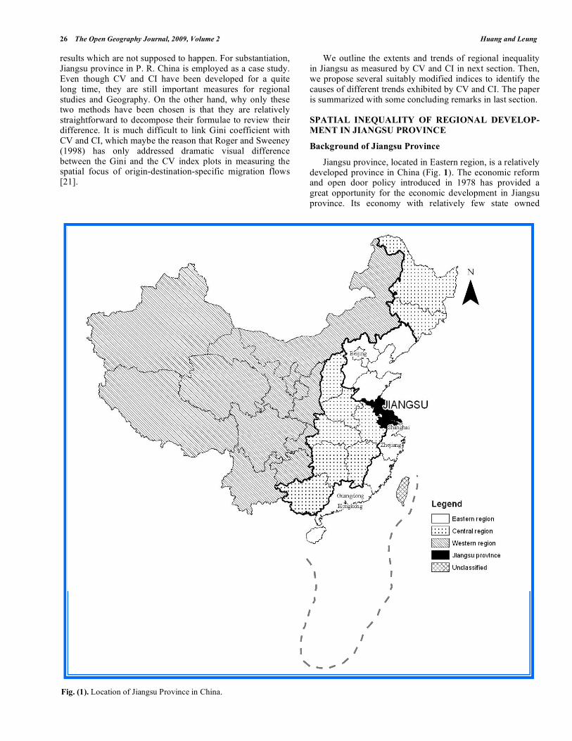
Jiangsu province, located in Eastern region, is a relatively developed province in China (Fig. 1). The economic reform and open door policy introduced in 1978 has provided a great opportunity for the economic development in Jiangsu province. Its economy with relatively few state owned

Fig. (1). Location of Jiangsu Province in China.

A Comparison of CV and CI The Open Geography Journal, 2009, Volume 2 27

enterprises but many collective enterprises forms a conducive environment for the development of a market economy. Thus, Jiangsu province has played an increasingly important role in China’s economy. Currently, Jiangsu province is one of the fastest growing provinces and is one of a few provinces with the fastest growing industrial sector as well as the most productive agricultural sector in China [22]. Even though Jiangsu province has experienced tremendous economic development in the past two decades, there are still significant regional differentials among its regional-level units, its prefecture-level units as well as its county-level units [18, 23]. Indeed, Jiangsu province provides a good case to study regional development within a province since it is a veritable microcosm of China and its significant regional inequalities at different spatial scales (see for examples, [24-29]). It is also useful to examine regional inequality in Sichuan, Yunnan or Guizhou Province as a typical case of less developed areas in China. This will be done in further research.

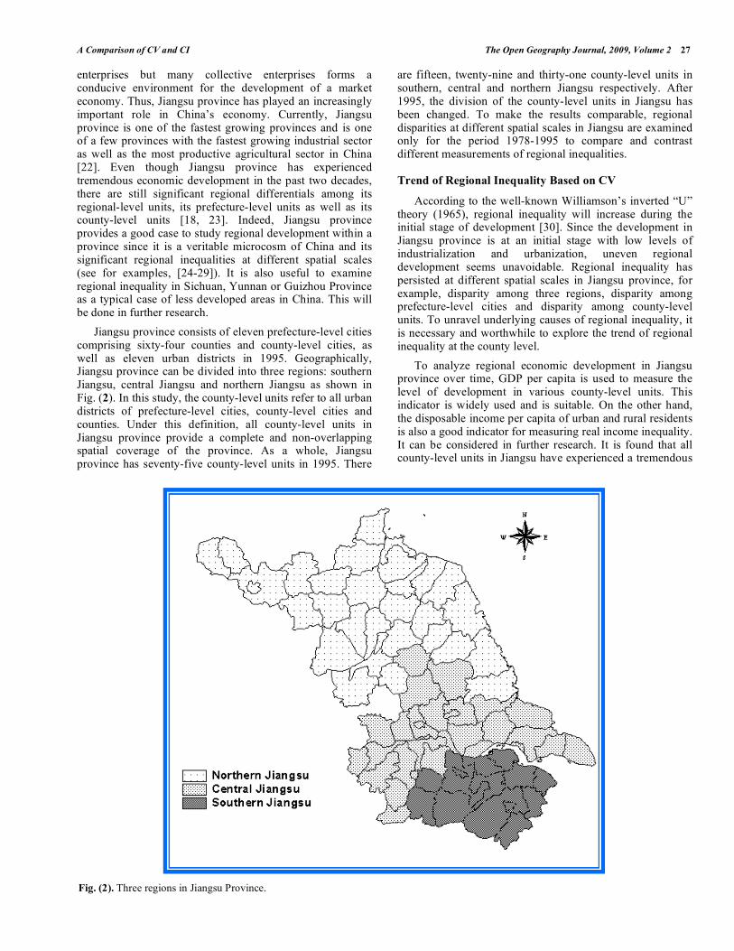
Jiangsu province consists of eleven prefecture-level cities comprising sixty-four counties and county-level cities, as well as eleven urban districts in 1995. Geographically, Jiangsu province can be divided into three regions: southern Jiangsu, central Jiangsu and northern Jiangsu as shown in Fig. (2). In this study, the county-level units refer to all urban districts of prefecture-level cities, county-level cities and counties. Under this definition, all county-level units in Jiangsu province provide a complete and non-overlapping spatial coverage of the province. As a whole, Jiangsu province has seventy-five county-level units in 1995. There

are fifteen, twenty-nine and thirty-one county-level units in southern, central and northern Jiangsu respectively. After 1995, the division of the county-level units in Jiangsu has been changed. To make the results comparable, regional disparities at different spatial scales in Jiangsu are examined only for the period 1978-1995 to compare and contrast different measurements of regional inequalities.

Trend of Regional Inequality Based on CV

According to the well-known Williamson’s inverted “U” theory (1965), regional inequality will increase during the initial stage of development [30]. Since the development in Jiangsu province is at an initial stage with low levels of industrialization and urbanization, uneven regional development seems unavoidable. Regional inequality has persisted at different spatial scales in Jiangsu province, for example, disparity among three regions, disparity among prefecture-level cities and disparity among county-level units. To unravel underlying causes of regional inequality, it is necessary and worthwhile to explore the trend of regional inequality at the county level.

To analyze regional economic development in Jiangsu province over time, GDP per capita is used to measure the level of development in various county-level units. This indicator is widely used and is suitable. On the other hand, the disposable income per capita of urban and rural residents is also a good indicator for measuring real income inequality. It can be considered in further research. It is found that all county-level units in Jiangsu have experienced a tremendous

Fig. (2). Three regions in Jiangsu Province.


increase in GDP per capita since 1978. Besides the growth, regional inequality in terms of GDP per capita in the reform period was also very obvious [18]. The coefficient of variation is adopted to measure the degree of regional inequality. Its formula is as follows:

( )

0

2

0/

Y

nYyCV

i= (1)

where yi is GDP per capita of county-level unit i in Jiangsu province, Y0 is the mean of yi, i.e. Y0 = (1/n) yi, and n is the number of county-level units in Jiangsu province.

Regional inequality in terms of CV among the seventy-five county-level units over the period 1978-1995 is shown in Fig. (3). According to its trend, the whole period can be divided into three subperiods: 1978 to 1984, 1985 to 1991 and 1992 to 1995. During the period of 1978-1984, the coefficient of variation decreased gradually from 94.39 percent to 71.69 percent indicating that regional inequality among all 75 county-level units was decreased. This period was the first stage of reform under the open door policy in Jiangsu province. The emphasis of reform at this stage was in rural areas where the family responsibility system was introduced and the commercial production was stimulated. The Sunan (South Jiangsu) Model with characteristics of cooperative development in farming, poultry, manufacturing and export emerged in this period. As a result of open door and reform policies, especially the rural policies, Jiangsu province experienced comprehensive development. Non-agricultural economic activities, especially township and village enterprises (TVEs), bloomed all over Jiangsu province. Therefore, the development in rural areas was faster than that in urban areas. Due to comprehensive

development, the degree of regional inequality, especially between urban and rural areas, was reduced.

During the period of 1985-1991, the trend of inequality showed a flat U-shaped pattern with the highest in 1985 and the lowest in 1988. The period matched nicely the second stage of reform in Jiangsu province which shifted the emphasis of reform from rural to urban areas. Various enterprises in urban areas were given much autonomy power and many horizontal economic linkages were developed to improve economic efficiency. Relatively developed areas grew faster than less developed areas in the latter part of this period. As a result, regional inequality of GDP per capita was reverted from declining slowly to increasing slowly.

During the first few years of the final period, regional inequality increased very rapidly and reached a peak in 1993. Due to the implementation of a coordinated regional development policy in China in 1992 [31], regional inequality started to decline after 1993. In conclusion, regional inequality within Jiangsu province, in terms of GDP per capita, is quite noticeable and it, contrary to stable trends of inter-provincial and inter-regional disparities in China found earlier [32], has fluctuated quite significantly in a wave-like trend. Nevertheless, as a whole, regional inequality based on CV declined slightly in Jiangsu province from 1978 to 1995.

Trend of Economic Concentration Based on CI

To further analyze the economic growth and consequent changes in spatial patterns, the Hoover concentration index [33, 34] is employed to identify and measure the process of economic concentration in terms of GDP in space within Jiangsu province. The formula to calculate the index is as follows:

0.00

0.20

0.40

0.60

0.80

1.00

1978

1979

1980

1981

1982

1983

1984

1985

1986

1987

1988

1989

1990

1991

1992

1993

1994

1995 Year

Coefficient

CV

Regression line of CV

CI

Regression line of CI

Fig. (3). Regional inequalities of GDP per capita based on CV and CI and their trends over the time in Jiangu.


CI = [ |ti* - ni

*|]/2 (2)

where ti* is the percentage share of GDP, and ni

* is the

percentage share of population in county-level unit i of the province. The Hoover concentration index varies between 0 and 1. If CI = 0, the spatial distribution of GDP is even. If CI = 1, the spatial distribution is extremely uneven and GDP is concentrated on one unit. Thus, the larger is the Hoover concentration index, the higher is the degree of concentration or unevenness. Fig. (3) also shows the trend of the geographical concentration of Jiangsu province’s economy over the period of 1978-1995 based on CI. The degree of spatial concentration of economic activities changed greatly from 1978 to 1995. CI increased from 0.267 in 1978 to 0.345 in 1993, and then decreased to 0.313 in 1995. The generally increasing trend of CI means increasing regional inequality in Jiangsu province until 1993.

Comparing the trends of regional inequality exhibited by the Hoover concentration index and the coefficient of variation using the same set of spatial units in Jiangsu province in the period of 1978-1995, it is clear that the two indicators show very different trends, especially in the initial years of the period. To further substantiate this observation, regressions of CI and CV on time have been performed and the statistical findings are summarized as follows:

CV = 19.140-0.009252 Time (3.101) (-2.978)

CI = -8.399+0.004368 Time (-4.295) (4.438)

The numbers in brackets are t-statistics of the estimated parameters. The regression equations are significant at 0.001 level. It can be observed that CV and CI show significantly different trends in the same set of data (see regression lines of CV and CI in Fig. 3).

It should, however, be noted that both CV and CI are supposedly measures of regional inequality showing similar trends. It is of concern that they could show opposite trends for the same set of data. To find out the cause for such a discrepancy between these two measures is important for the study of regional disparity. In the following section, the similarity and dissimilarity of these two measures will be compared and contrasted to identify the reasons for their uncovering different trends of regional inequality among the same set of spatial units in Jiangsu province.

Exploring the Difference Between CV and CI

Based on the analysis results above, it is clear that using different methods with the same intention to measure regional inequality may lead to inconsistent conclusions. While the trend of regional inequality in Jiangsu province was shown declining in the period of 1978-1995 by the CV measure, the trend, on the contrary, was shown rising in the same period by the CI measure. We argue that such a contrasting difference may be caused by two factors. One is the population weight for each area in the CI measure. The other is the absolute deviation of the original data from the mean. Generally, the absolute deviation from the mean is greater in a whole region than in one of its sub-regions. Geographically, Jiangsu province is divided into various sub-regions such as urban and rural areas, southern, central and

northern regions. Therefore, different from the case of the whole Jiangsu province, CV and CI for a sub-region in Jiangsu province might have very similar results as the absolute deviation from the mean is much smaller. A detailed analysis is made in the following subsections.

The Effect of the Population Weight

Fig. (3) shows the trends of regional inequality among the county-level units in Jiangsu province obtained by applying CV and CI on the same set of data. It is apparent that these two measures show considerably different trends even though their patterns are similar to some extent. The general trend of CV is downward while the trend of CI is slightly upward (see regression lines in Fig. 3). However, the curves of these two trends are relatively consistent after 1984. A scrutiny of formulae (1) and (2) shows that CV evidently measures the variance of GDP per capita, and CI measures the process of concentration in term of GDP and population.

Though both indices measure the extent of regional inequality, a direct comparison is difficult to make. By some suitable manipulation, however, we can unravel some revealing comparisons. Using ti

* = (gi / G) 100 and ni

* = (pi /

P) 100, where gi means the amount of GDP in county-level unit i and pi means population in county-level unit I, CI can be rewritten as:

CI = ti* ni

* / 2 =giG

100piP

100 / 2

= 50piG

gipi

G

P

(3)

Let:

yi =gipi

(4)

Then, the GDP per capita, Y, for the whole province can be expressed as:

Y =G

P (5)

where G means the total GDP and P means the total population in Jiangsu province. Replacing gi/pi and G/P by yi and Y respectively, formula (3) becomes:

CI =piG

yi Y = 50pi / P

G / Pyi Y

= 50piP

yi Y

Y

(6)

On the other hand, the formula for CV can also be rewritten as:

CV =yi Y0( )

2

Y0 n (7)

Comparing formulae (6) and (7) for CI and CV respectively, the main differences between CI and CV can be observed. First, CI is affected by the population weight of


pi/P. This means that a similar deviation of unit i, yi-Y, or yi-Y0, with a larger share of the total population, pi/P, is more important in the CI index than in the CV index. Difference in the population weight of a unit is one of the reasons causing the difference in the measurement of regional inequality.

Second, Y in (6) and Y0 in (7) have different meanings. Namely, Y is the GDP per capita (population weighted average of GDP per capita in all areas) in Jiangsu province, i.e., Y = G/P = piyi / pi, and Y0 is the arithmetic average of GDP per capita of all county-level units in Jiangsu, i.e., Y0= yi/n. The difference between Y and Y0 will result in difference between CV and CI.

Third, CV is proportional to the squared deviation from the mean (yi-Y0) of the original data while CI is just proportional to the absolute deviation from the mean (yi-Y0). This means that areas with larger deviation (yi-Y0) are much more important in the CV measure than the CI measure. Such difference again will result in difference between CV and CI.

To unravel the real impact of the above differences in two indices on the overall trend of regional inequality, some modified versions of the CI are proposed to capture the effects of the above differences on CV and CI. First, to eliminate the difference caused by the use of Y instead of Y0, Y is replaced by Y0 in formula (6) and a revised CI, CI(2), is constructed as follows:

CI(2) = 50piP

yi Y0Y0

(8)

Applying the revised concentration index CI(2) to 75 county-level units in Jiangsu province, the result is obtained and depicted in Fig. (4). Comparing the curves of CI and CI(2), it can be observed that the trend of CI(2) shows a slight decline in the initial years and is closer to that of CV in Fig. (3) and the range of CI(2) is smaller than that of the original index, CI. Thus, it seems that using Y0 to replace Y does have some effects on the behavior of CI. Such effects are nevertheless quite trivial.

One further modification of the CI measure is to remove the effect of population weight. It is done by replacing the population in each area in formula (6) with the average population of an area. Thus another revised index CI(3) is constructed as follows:

CI(3) = 50P0P

yi Y

Y

= 50P / n

P

yi Y

Y

=50

n

yi Y

Y

(9)

where the population pi in a county-level unit i in formula (6) is replaced by the population mean P0, and n is the number of county-level units. Therefore, P0 = pi / n = P / n.

Applying formula CI(3) to the data of the 75 county-level units in Jiangsu province, we obtain the result which is shown in Fig. (4). The difference between CI and CI(3) is that the population weight is removed in CI(3). The result shows that the range of CI(3) is much flatter than that of CI. One important feature is that the trend of CI(3) has a more apparent decline than that of CI and CI(2). Thus, it can be said that the population weight pi/P actually is a significant cause of the different trends of CI and CV. However, the above two revisions of CI still cannot account for all difference between CV and CI. The remaining reason is likely related to the fact that (yi-Y0) is raised to a power of two in CV at one stage of calculation. Its effect will also depend on the deviation from the mean for various units. This issue is addressed in details in the following subsection.

The Effect of the Deviation from the Mean

It is suspected that the characteristics of the data set, such as range and deviation from the mean, may also be a plausible factor causing different behavior of CV and CI. Such effect, if any, can be traced in two ways. First, the absolute deviation of

0.22

0.24

0.26

0.28

0.30

0.32

0.34

0.36

1978

1979

1980

1981

1982

1983

1984

1985

1986

1987

1988

1989

1990

1991

1992

1993

1994

1995

Year

CI CoefficientCI

CI(2)

CI(3)

Fig. (4). Regional inequality of GDP per capita based on CI and adjusted measures of CI(2)and CI(3) in Jiangsu.


GDP per capita from the mean in each of the 75 county-level units in the period of 1978-1995 is examined and Fig. (5) depicts the maximum five deviations for each year in the period of 1978-1995. It is apparent that the maximum five absolute deviations decreased from 1978 to 1995. Thus, the deviation of GDP per capita from the mean has decreased in this period. Since CV is related to the square of the absolute deviation, |yi - Y0|, the effect of |yi - Y0| on CV is doubled. The larger is the absolute deviation, the disproportionally bigger the value of CV becomes. As a result, a larger absolute deviation has a more substantial impact on the value of CV. Based on the above discussion, the declining trend of large absolute deviations from the mean in the data set revealed in Fig. (5) must have contributed to the declining trend of CV of GDP per capita among the 75 county-level units in Jiangsu in 1978-1995.

CI, on the other hand, is also positively related to the absolute deviation in the data, but the absolute deviation has less impact on the value of CI as CI is only proportional to the absolute deviation. CI does not have the same behavior of CV and actually shows an opposite trend to that of CV in the period of 1978-1995.

To further test the above argument, the formula of CV is modified so that the absolute deviation is raised to the powers of 1.75, 1.5, 1.25 and 1 instead of the original power of 2 as follows:

CV (1.75) =yi Y0

1.75/ n( )

11.75

Y0 (10)

CV (1.5) =yi Y0

1.5/ n( )

11.5

Y0 (11)

CV (1.25) =yi Y0

1.25/ n( )

11.25

Y0 (12)

CV (1) =yi Y0 / n( )Y0

(13)

Apparently the differences among formulae CV(1.75), CV(1.5), CV(1.25) and CV(1) are that the absolute deviation from the mean, |yi - Y0|, is raised to different magnitudes and these formulae become closer and closer to the CI formula but further and further away from the CV formula as the power decreases from 1.75 to just 1. If being raised by different magnitudes has some effects on the calculated results, the trends obtained by CV(1.75), CV(1.5), CV(1.25) and CV(1) in Jiangsu province should be located between the trends of CV and CI. According to the previous discussion, it is also expected that they differ most significantly in the initial years of the period when the deviations from the mean are larger. Fig. (6) shows various trends of CV, CV(1.75), CV(1.5), CV(1.25) and CV(1) in Jiangsu province. Comparing Fig. (4) with Fig. (6), it is obvious that the trends of CV(1.75), CV(1.5), CV(1.25) and CV(1) are in-between the patterns of CV and CI. Actually, the pattern of CV(1) is very close to that of CI(3). The difference between them is just the difference between Y and Y0, and a constant factor of 50/n (i.e. 50/75 in this case). Clearly, the trend of CV has been substantially influenced by large absolute deviations in the data set.

In addition to the examination of the difference between CV and CI among 75 county-level units for Jiangsu as a whole, it is also useful to scrutinize the difference between CV and CI among sub-regions such as rural and urban areas in Jiangsu. Generally, the absolute deviations of GDP per capita among urban districts of prefecture-level cities were bigger than those of GDP per capita among counties and county-level cities. Thus, all county-level units in Jiangsu province are divided into two groups of urban and rural areas respectively. Urban area includes those county-level units that are urban districts of prefecture-level cities and rural area includes those county-level units that are counties and county-level cities. The deviations of GDP per capita among the county-level units in either urban or rural area are definitely smaller than the deviations of GDP per capita among all county-level units in Jiangsu province.

1.00

1.50

2.00

2.50

3.00

3.50

4.00

1978

1979

1980

1981

1982

1983

1984

1985

1986

1987

1988

1989

1990

1991

1992

1993

1994

1995

Year

Abs. deviationMax 1

Max 2

Max 3

Max 4

Max 5

Fig. (5). Five largest absolute deviations of GDP per capita in Jiangsu.


To further investigate the different trends between CV and CI in the context of a reduction in the spatial coverage, these two measures are used to examine the regional inequality among the county-level units in urban and rural areas in Jiangsu province respectively. Fig. (7) shows the trends of regional inequality based on CV and CI within urban and rural areas. It is interesting to note that opposite to the case of the whole province, the trends of CV and CI are very similar among county-level units within the urban or rural area. As mentioned above, the fact that there is no dominant large absolute deviation in the data set of either urban or rural area is the main reason.

To examine further, the county-level units in the whole Jiangsu province is divided into three groups, i.e., southern, central and northern regions. To compare and contrast the behavior of CV and CI in each of the three regions, we obtain the results depicted in Fig. (8). It appears that the

trends of CV and CI are less consistent for each of the three regions than those for both urban and rural areas. However, they are much more consistent than the trends of CV and CI among all the county-level units in the whole province. Similar to the case of urban or rural area, the main reason is that the deviations in the data set of any one region are smaller than the deviations in the data set for all the county-level units of the province. It is clear that when CV and CI are calculated from a spatial data set where no dominant absolute deviations exist among the spatial units, the trends of regional inequality revealed by CV and CI tend to be much more consistent.

CONCLUSION

As discussed, many measures have been used in the study of regional inequality, such as the coefficient of variation and Hoover concentration index. However,

0.50

0.60

0.70

0.80

0.90

1.00

1978

1979

1980

1981

1982

1983

1984

1985

1986

1987

1988

1989

1990

1991

1992

1993

1994

1995

Year

CV CoefficientCV

CV(1.75)

CV(1.5)

CV(1.25)

CV(1)

Fig. (6). The trends of regional inequality measured by various modified CVs in Jiangsu.

0.10

0.20

0.30

0.40

0.50

0.60

0.70

0.80

0.90

1978

1979

1980

1981

1982

1983

1984

1985

1986

1987

1988

1989

1990

1991

1992

1993

1994

1995

Year

CoefficientCV-urban

CV-rural

CI-urban

CI-rural

Fig. (7). Trends of CV and CI in urban and rural areas of Jiangsu in terms of GDP per capita.


opposite results are often obtained from different quantitative measures which are meant to show the same trend. An attempt is made in this paper to explain how two commonly used measures, CV and CI, can produce completely contrasting results. We have demonstrated in this paper such an irony in the study of regional inequality in Jiangsu province. Further case studies will be conducted to compare the regional inequalities in Western regions such as Sichuan, Yunnan or Guizhou.

Regional economic development in Jiangsu province was uneven in terms of GDP per capita during the period of 1978-1995. However, when CV and CI are used, they reveal different trends of regional inequality in Jiangsu province. In terms of CV, regional inequality of GDP per capita took on a declining trend with intermittent fluctuations. Nevertheless, CI increased steadily from 1978 to 1993 and then decreased towards 1995. By constructing some suitably modified indices, we have found the main reasons for such inconsistent trends of regional inequality. Comparison of the trends exhibited by these indices together with CV and CI helps to explain the difference between CV and CI.

It has been unraveled that population weight and deviation from the mean in the data set are two main causes leading to different trends of regional inequality manifested by CV and CI. Differing from CV, CI is the sum of population weighted relative deviations. To reveal the impact generated by such a difference, population weight for each areal unit is replaced by the average population of all units. The contribution of population weight to the difference between CV and CI has thus been identified.

In terms of the effect of deviations from the mean in the data set, it is found that CV is proportional to the squared absolute deviation of |yi - Y0|, while CI is just linearly related to |yi - Y0|. Thus, the deviation from the mean, |yi - Y0|, has a much larger effect on CV than on CI, especially when the deviation is very large. This argument has been further confirmed by several proposed indices with varying exponent terms on the CV. It has been demonstrated that the trends of regional inequality gradually change from CV to CI.

In terms of the spatial coverage on which data are collected, CV and CI appear to be more similar when spatial coverage moves from the whole province to urban or rural area and to any one of the three sub-regions. As the deviations in the data set for a sub-region is much smaller than that for the whole province, the difference between CV and CI becomes smaller. It is a further indication of the significant impact of the absolute deviations from the mean, |yi - Y0|, on the difference between CV and CI.

As a conclusion, though both CV and CI are two kinds of measurement intended to show the same pattern of regional inequality, they may show opposite results when they are applied to specific cases. While CI takes the population weight of each areal unit into consideration, areal units with large deviations from the mean will generate much greater impact on CV since it gives more weight to large absolute deviations in the data by taking a square. Thus, CV and CI may display different trends when a few large absolute deviations dominate the data set. Therefore, measurements of regional inequality, CV and CI in particular, should not be used indiscriminately. Otherwise, dubious conclusion might be drawn. From this research, it appears that CI is a more appropriate method for measuring regional disparity when population weight of each areal unit matters. When larger deviation from the mean is the focus in the study of regional disparity, CV appears to be more appropriate.

ACKNOWLEDGEMENT

We would like to thank the two anonymous reviewers for their helpful comments on an earlier draft of this paper.

REFERENCES

[1] Hare D, West LA. Spatial patterns in China's rural industrial

growth and prospects for the alleviation of regional income inequality. J Comp Econ 1999; 27: 475-97.

[2] Zheng F, Xu L, Tang B. Forecasting regional income inequality in China. EJOR 2000; 124: 243-54.

[3] Wei YH. Regional inequality in China. Prog Hum Geogr 1999; 23(1): 49-59.

[4] Gustafsson B, Li S. Income inequality within and across counties in rural China 1988 and 1995. J Dev Econ 2002; 69: 179-204.

[5] Ron D, Tian X. China’s inter-provincial disparities an explanation. Commun Post-Commun Stud 1999; 32: 211-24.

0.00

0.20

0.40

0.60

0.80

1.00

1978

1979

1980

1981

1982

1983

1984

1985

1986

1987

1988

1989

1990

1991

1992

1993

1994

1995

Year

Coefficient CV-S CV-C CV-N

CI-S CI-C CI-N

Fig. (8). Trends of CV and CI in the southern, central and northern Jiangsu in terms of GDP per capita.


[6] Lardy NR. Regional growth and income distribution in China. In:

Dernberger RF, Ed. China’s development experience in comparative perspective. Cambridge: Harvard University Press

1980; pp. 153-90. [7] Paine S. Spatial aspects of China development: issues, outcomes

and policy 1949-79. J Dev Stud 1981; 17: 132-95. [8] Tsui KY. Decomposition of China’s regional inequalities. J Comp

Econ 1993; 17: 600-27. [9] Lyons TP. Interprovincial disparities in China: output and

consumption, 1952-1987. Econ Dev Cult Change 1991; 39(3): 471-506.

[10] Jian T, Sachs JD, Warner AM. Trends in regional inequality in China. China Econ Rev 1996; 7(1): 1-21.

[11] Tsui KY. Economic reform and interprovincial inequalities in China. J Dev Econ 1996; 50: 353-68.

[12] Fan CC. Of belts and ladders: state policy and uneven regional development in post -Mao China. AAG 1995; 85(3): 421-49.

[13] Shen J. Urban and regional development in post-reform China: the case of Zhujiang delta. Prog Plann 2002; 57(2): 91-140.

[14] Yao SJ. Industrialization and spatial income inequality in rural China, 1986-92. Econ Transit 1997; 5(1): 97-112.

[15] Long G.Y. China’s changing regional disparities during the reform period. Econ Geogr 1999; 75(1): 59-70.

[16] Zhao XB. Spatial disparities and economic development in China, 1953-92: a comparative study. Dev Change 1996; 27(1): 131-63.

[17] Li SM. China’s changing spatial disparities: a review of empirical evidence. In: Li SM, Tang WS, Eds. China’s regions, polity, and

economy. Hong Kong: CUHK 2000; pp. 155-86. [18] Huang Y. Decomposition of regional inequalities in Jiangsu since

1978. Asian Geogr 2002; 21(1&2): 145-58. [19] Ray D. Economic inequality. Development economics. New

Jersey: Princeton University Press 1998; 169-96. [20] Tian XW. Dynamics of development in an opening economy:

China since 1978. New York: Nova Science Publishers, Inc. 1998.

[21] Roger A, Sweeney S. Measuring the spatial focus of migration

pattern. Prof Geogr 1998; 50(2): 232-42. [22] Rozelle S, Jiang LY. Survival strategies and recession in rural

Jiangsu. Chin Environ Dev 1996; 6(1&2): 43-84. [23] Huang Y, Leung Y. Analysis of regional industrialisation in

Jiangsu Province using geographically weighted regression. J Geogr Syst 2002; 4: 233-49.

[24] Ma LJC, Fan M. Urbanisation from below: the growth of towns in Jiangsu, China. Urban Stud 1994; 31(10): 1625-45.

[25] Fan CC. Spatial impacts of China’s economic reforms in Jiangsu and Guangdong provinces. Chin Environ Dev 1995; 6(1&2): 85-

116. [26] Su SJ, Veeck G. Foreign capital acquisition by rural industries in

Jiangsu. Chin Environ Dev 1995; 6(1&2): 169-92. [27] Wei YH, Fan CC. Regional inequality in China: a case study of

Jiangsu province. Prof Geogr 2000; 52(3): 455-69. [28] Huang Y. Spatial dynamics of industrialization in Jiangsu. J Chin

Geogr 2000; 10(2): 129-40. [29] Wei YH. Beyond the Sunnan model: trajectory and underlying

factors of development in Junshan, China. Environ Plann A 2002; 34: 1725-47.

[30] Williamson JG. Regional inequality and the process of national development: a description of the pattern. Econ Dev Cult Change

1965; 13(4): 3-45. [31] Lu DD, Sit FS. The report of regional development in China in

1997 (In Chinese), Beijing: Commercial Press 1997. [32] Wei YH, Ma LJC. Changing patterns of spatial inequality in China:

1952-1990. Third World Plann Rev 1996l; 18(2): 177-91. [33] Isard W. Methods of regional analysis. Massachusetts: The M.I.T.

Press 1960. [34] Weng Q. Local impacts of the post-Mao development strategy: the

case of the Zhujiang delta, southern China. Int J Urban Reg Res 1998; 22(3): 425-42.

Received: April 10, 2009 Revised: September 5, 2009 Accepted: September 10, 2009

© Huang and Leung; Licensee Bentham Open.

This is an open access article licensed under the terms of the Creative Commons Attribution Non-Commercial License (http://creativecommons.org/licenses/by-

nc/3.0/) which permits unrestricted, non-commercial use, distribution and reproduction in any medium, provided the work is properly cited.

measuring regional inequality: a comparison of coefficient of variation … · 2016-11-22 ·...

Documents