mechanical and electrical properties of micro

MECHANICAL AND ELECTRICAL PROPERTIES OF MICRO-ARCHITECTURED

CARBON NANOTUBE SHEET

BY

YUE LIANG

THESIS

Submitted in partial fulfillment of the requirements

for the degree of Master of Science in Mechanical Engineering

in the Graduate College of the

University of Illinois at Urbana-Champaign, 2016

Urbana, Illinois

Adviser:

Professor Sameh Tawfick

ii

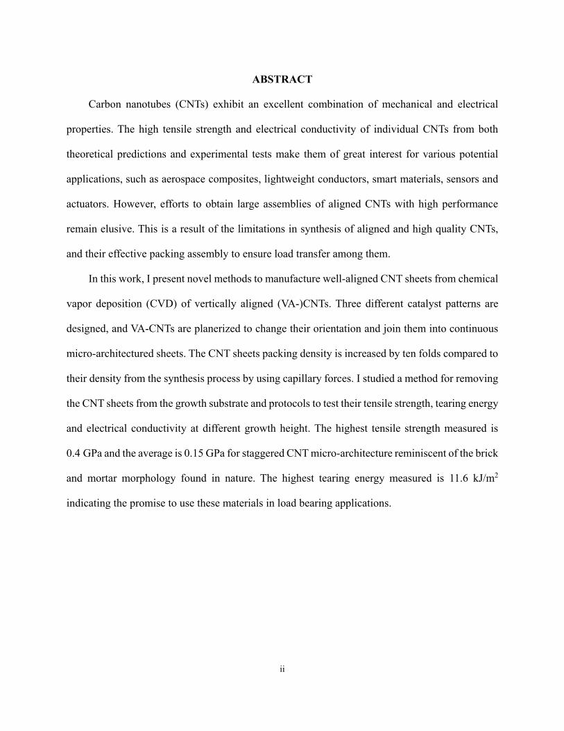
ABSTRACT

Carbon nanotubes (CNTs) exhibit an excellent combination of mechanical and electrical

properties. The high tensile strength and electrical conductivity of individual CNTs from both

theoretical predictions and experimental tests make them of great interest for various potential

applications, such as aerospace composites, lightweight conductors, smart materials, sensors and

actuators. However, efforts to obtain large assemblies of aligned CNTs with high performance

remain elusive. This is a result of the limitations in synthesis of aligned and high quality CNTs,

and their effective packing assembly to ensure load transfer among them.

In this work, I present novel methods to manufacture well-aligned CNT sheets from chemical

vapor deposition (CVD) of vertically aligned (VA-)CNTs. Three different catalyst patterns are

designed, and VA-CNTs are planerized to change their orientation and join them into continuous

micro-architectured sheets. The CNT sheets packing density is increased by ten folds compared to

their density from the synthesis process by using capillary forces. I studied a method for removing

the CNT sheets from the growth substrate and protocols to test their tensile strength, tearing energy

and electrical conductivity at different growth height. The highest tensile strength measured is

0.4 GPa and the average is 0.15 GPa for staggered CNT micro-architecture reminiscent of the brick

and mortar morphology found in nature. The highest tearing energy measured is 11.6 kJ/m2

indicating the promise to use these materials in load bearing applications.

iii

ACKNOWLEDGMENTS

It is my great honor to have the opportunity to work with Prof. Sameh Tawfick. I could not

have asked for a better mentor than him. I was extremely lucky when I started my undergraduate

research with him three years ago. My research ability grows day by day under his influence. It’s

his enthusiasm, comprehensiveness, and advising that accompanies me for the past three years and

helped me develops to a mature researcher.

I would like to thank my colleagues in Kinetic Material Group: Ping-Ju Chen, Kaihao Zhang,

Matt Robertson, Matt Poss, Alex Pagano, and Jonathan Bunyan. I could not have completed my

journey at UIUC without your help, your enthusiasm, and your humors around the lab.

I am thankful to my loved one, David, whom accompanied me throughout my college life at

UIUC, whom supported me without complaints through all the good and bad days. I could not

imagine my college life without yours accompany.

I am thankful to my grandparents, my aunts and uncles, and my cousins, whom supported me

and trusted in me all the time.

Last but not least, I would like to thank my parents. Thank you for your support throughout

my life. Thank you for your unconditional love.

iv

TABLE OF CONTENTS

CHAPTER 1 INTRODUCTION .................................................................................................... 1

1.1 Introduction to Carbon Nanotube ..................................................................................... 1

1.2 Single-walled carbon nanotube and multi-walled carbon nanotube ................................. 1

1.3 Mechanical Property of Carbon Nanotube ....................................................................... 2

1.4 Electrical Property of Carbon Nanotube ........................................................................... 3

CHAPTER 2 METHODS ............................................................................................................... 4

2.1 Deposition of catalyst ....................................................................................................... 4

2.2 Carbon nanotube synthesis ............................................................................................... 8

2.3 Patterns of carbon nanotube ............................................................................................ 12

2.4 Transfer of structured carbon nanotube .......................................................................... 15

2.5 Electrical Test preparation .............................................................................................. 21

2.6 Mechanical Test preparation ........................................................................................... 23

CHAPTER 3 CAPILLARY FORCE MODELING ...................................................................... 25

3.1 Capillary force between carbon nanotubes ..................................................................... 25

3.2 Capillary force modeling using finite element analysis .................................................. 26

3.3 Algorithm of modeling .................................................................................................... 28

3.4 Capillary force acting against carbon nanotubes ............................................................ 34

3.5 Capillary force acting along the outline of carbon nanotubes ........................................ 38

3.6 Discussion of FEA modeling of capillary forces ............................................................ 41

CHAPTER 4 RESULTS AND DISCUSSION ............................................................................. 42

4.1 Thickness Characterization ............................................................................................. 42

4.2 Electrical Conductivity ................................................................................................... 45

4.3 Mechanical Strength ....................................................................................................... 45

4.4 Fracture Toughness of Staggered Pattern ........................................................................ 46

4.5 Results of Line Pattern (30 x 400) .................................................................................. 47

4.6 Results of Line Pattern (50 x 400) .................................................................................. 51

4.7 Results of Staggered Pattern ........................................................................................... 55

4.8 Fractography of Broken Samples .................................................................................... 63

4.9 Discussion and Comparison of Different Patterns .......................................................... 65

CHAPTER 5 CONCLUSIONS AND FUTURE WORK ............................................................. 66

v

APPENDIX ................................................................................................................................... 67

REFERENCES ............................................................................................................................. 81

1

CHAPTER 1 INTRODUCTION

1.1 Introduction to Carbon Nanotube

Carbon nanotubes (CNT) are cylindrical shaped structure with hexagonally packed

carbon-carbon bonds [1]. They can be visualized as a rolled-up graphene sheet. There are

two types or CNTs, single-walled carbon nanotubes (SWCNT) and multi-walled carbon

nanotubes (MWCNT). Upon its discovery, CNT exhibited extraordinary mechanical and

electrical properties. However, the properties of CNTs are limited by their synthesis and

alignment. Although the longest individual CNT that researchers synthesized is 550 mm [2],

eventually the growth terminates and this motivates the research to obtain dense, bulk and

well-aligned CNT material.

Because of their potential applications, researchers have focused on understanding and

enhancing the fundamental properties of CNT assemblies in the form of yarns and sheets.

In this thesis, I mainly focus on studying the mechanical and electrical properties of CNT

by synthesizing vertically-aligned (VA-)CNTs and transforming them to horizontally-

aligned (HA-)CNTs sheet by mechanically folding, joining, packing and releasing them

from the growth substrate.

1.2 Single-walled carbon nanotube and multi-walled carbon nanotube

SWCNT can be visualized as a rolled-up graphene layer, where each carbon atom is

covalently bonded to its neighboring carbon atom. These covalent bonds (σ-bond) result in

the strong mechanical property of CNT [1].

2

Multi-walled carbon nanotube (MWCNT) can be visualized as nested shells of

SWCNT. The interlayer bond is essentially the out-of-plane bond (π-bond), which are

weaker than the covalent bond [1]. These π-bond contributes to the interaction between the

layers of MWCNTs [1].

My work focused on MWCNTs. Mechanical and electrical properties of such CNTs are

discussed in the following sections.

1.3 Mechanical Property of Carbon Nanotube

Researchers have discovered impressive mechanical properties of CNTs. Both the

theoretical and experimental researches show high mechanical strength of SWCNTs and

MWCNTs [1].

The strength of CNTs could reach theoretical limit if defect-free [1]. These defects are

introduced during the synthesis process. The three main synthesis process CNTs are Arc-

discharge [3-5], laser ablation [6,7], and chemical vapor deposition (CVD) [8-10]. I used

chemical vapor deposition (CVD) to manufacture patterned VACNT and fold them to

HACNT sheets. The manufacturing process is mainly discussed in Chapter 2.

It is observed that, during loading process of tensile test, only the outermost shells of

MWCNTs are pulled apart [11]. The measured tensile strength of individual MWCNTs are

ranging from 11 to 63 GPa. Pan et al. [12] tested long ropes of aligned MWCNTs

synthesized by the CVD method, which gives a much lower value of tensile strength

(~ 1.72 GPa). The high discrepancy among different tests is resulted from the defects

introduced during the manufacturing process. Theoretical limits are reachable only in small

3

scale. When CNTs are manufactured to bulk materials, its properties are highly disrupted.

Vilatela et al. [13] modeled the strength of CNT fibers using experimental data and

computational simulations. It is observed that, during tensile test, CNTs fail due to shear

between neighboring fibrous elements instead of breakage of individual CNTs. This

observation is important especially for CNT sheet manufacture. In order to enhance the

tensile strength of CNT sheets, it is important to enhance the contact between individual

CNT fibers. In our approach, it is essential to increase the overlapping areas between each

CNT features. This will increase the shear contact between CNT fibers, which will in turn

enhance the tensile strength of our CNT sheets.

1.4 Electrical Property of Carbon Nanotube

CNTs also exhibit attractive electrical property. They can either be metallic or

semiconducting, Miao [14] was able to measure the electrical conductivity of pure CNT

yarns drawn from CNT forest after growth. In his work, he was able to get CNT yarns with

conductivity values ranging from 15 kS/m to 37 kS/m. A similar experiment of CNT yarns

spun directly from a furnace reported conductivity values of 500 kS/m [15]. The

discrepancy of conductivity values is resulted from two possible causes: the difference in

synthesis method and hence the defects density; and the inaccurate estimation of cross-

sectional area.

The focus of this work is to manufacture conductive CNT sheets with good mechanical

properties. The exact method is described in Chapter 2.

4

CHAPTER 2 METHODS

This chapter discusses the procedures that are taken to deposit catalysts for CNT

growth, CNT growth recipe, fabrication of the polymer transfer substrate used for VACNT

transfer, procedure of HACNT manufacture, and electrical property test and mechanical

property test preparation.

2.1 Deposition of catalyst

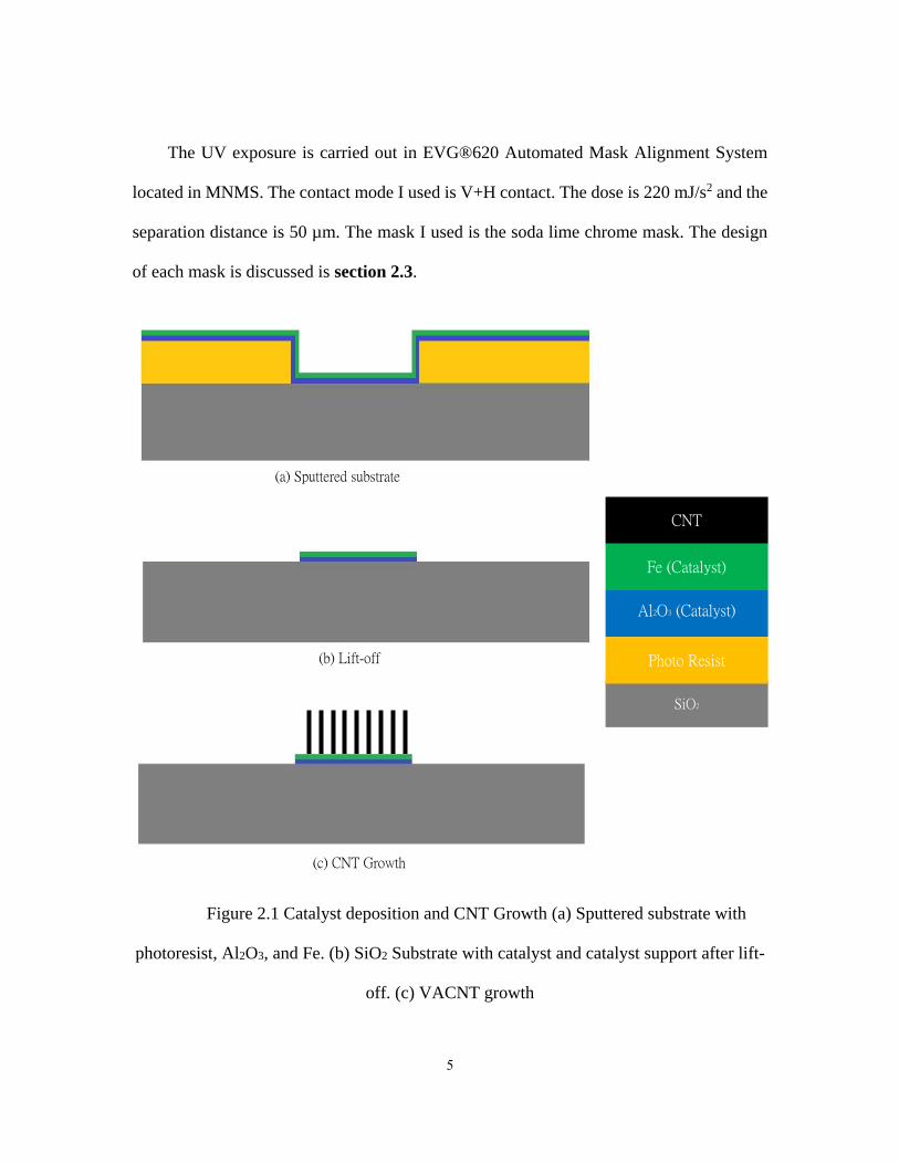
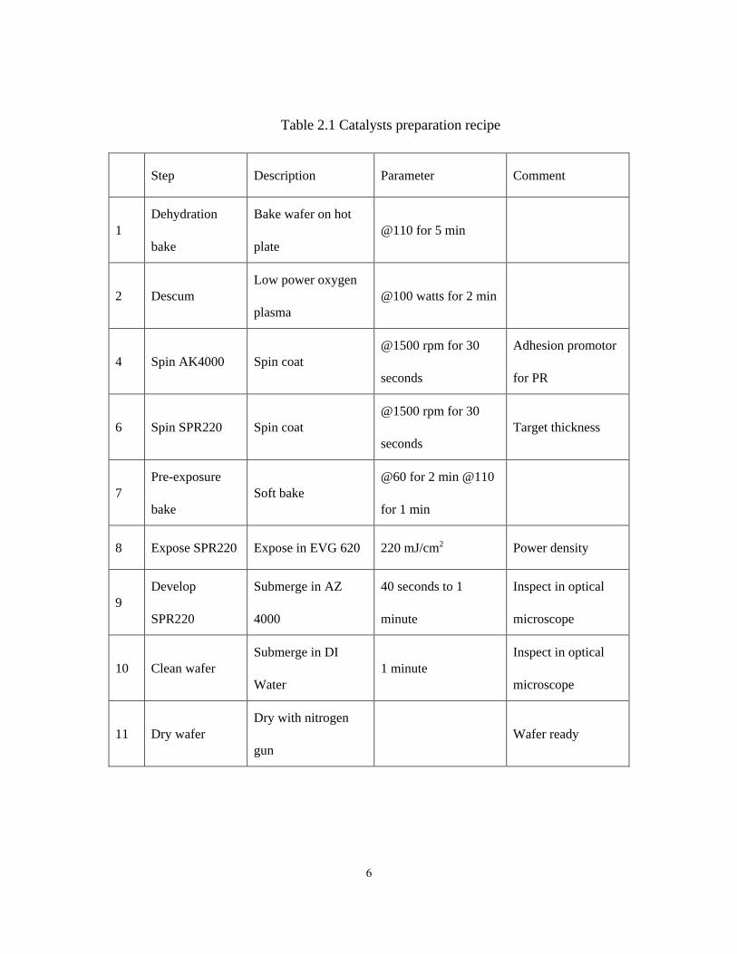
It requires several steps to prepare for a free-standing structured CNT sheet. First, a

substrate with patterned catalyst and catalyst support is manufactured using

photolithography in Micro-Nano-Mechanical Systems (MNMS) clean room. The complete

recipe is shown in Table 2.1 along with deposition procedure shown in Figure 2.1.

The process starts with (100) silicon dioxide coated wafers. These wafers are acquired

from WRS Materials Company. The wafer is spin coated with a thin layer of AP 3000

adhesion promotor at 3000 rpm for 30 seconds. AP 3000 functions as an adhesion layer.

Another thin layer of SPR 220 is then spin coated on top of AP 3000 also at 3000 rpm for

30 seconds. The recipe for spin coat of both layers is shown in Table 2.1.

Following spin coating is soft baking, where the wafer is baked at 60 for 2 minutes

and 110 for 1 minute.

5

The UV exposure is carried out in EVG®620 Automated Mask Alignment System

located in MNMS. The contact mode I used is V+H contact. The dose is 220 mJ/s2 and the

separation distance is 50 µm. The mask I used is the soda lime chrome mask. The design

of each mask is discussed is section 2.3.

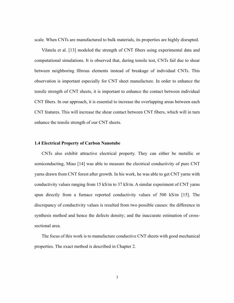
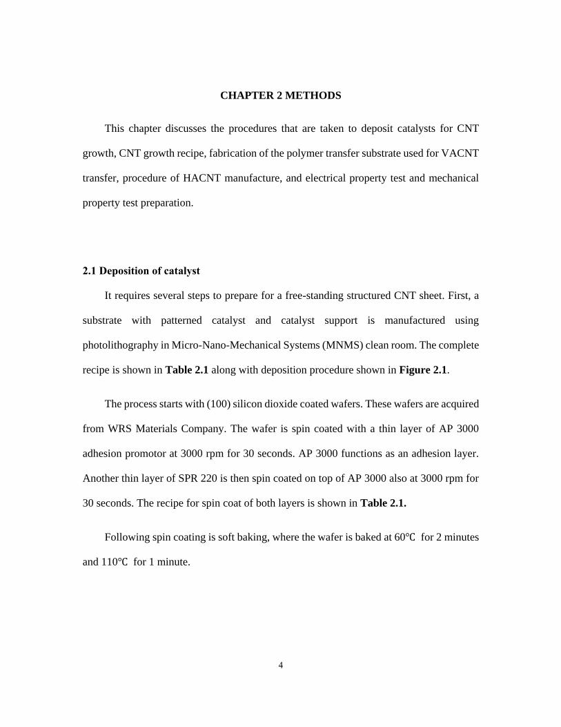
Figure 2.1 Catalyst deposition and CNT Growth (a) Sputtered substrate with

photoresist, Al2O3, and Fe. (b) SiO2 Substrate with catalyst and catalyst support after lift-

off. (c) VACNT growth

SiO2

Fe (Catalyst)

Al2O3 (Catalyst)

Support)

CNT

Photo Resist

(a) Sputtered substrate

(b) Lift-off

(c) CNT Growth

6

Table 2.1 Catalysts preparation recipe

Step Description Parameter Comment

1

Dehydration

bake

Bake wafer on hot

plate

@110 for 5 min

2 Descum

Low power oxygen

plasma

@100 watts for 2 min

4 Spin AK4000 Spin coat

@1500 rpm for 30

seconds

Adhesion promotor

for PR

6 Spin SPR220 Spin coat

@1500 rpm for 30

seconds

Target thickness

7

Pre-exposure

bake

Soft bake

@60 for 2 min @110

for 1 min

8 Expose SPR220 Expose in EVG 620 220 mJ/cm2 Power density

9

Develop

SPR220

Submerge in AZ

4000

40 seconds to 1

minute

Inspect in optical

microscope

10 Clean wafer

Submerge in DI

Water

1 minute

Inspect in optical

microscope

11 Dry wafer

Dry with nitrogen

gun

Wafer ready

7

The wafer is then developed in a fresh container filled with AZ400K with a ratio of

1:5 in volume to deionized (DI) water. A descum step (low power oxygen plasma) is

followed to remove any exposed remaining PR.

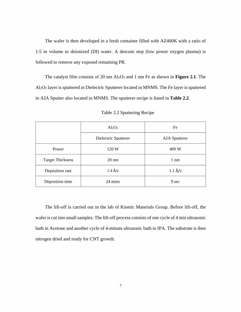
The catalyst film consists of 20 nm Al2O3 and 1 nm Fe as shown in Figure 2.1. The

Al2O3 layer is sputtered in Dielectric Sputterer located in MNMS. The Fe layer is sputtered

in AJA Sputter also located in MNMS. The sputterer recipe is listed in Table 2.2.

Table 2.2 Sputtering Recipe

Al2O3 Fe

Dielectric Sputterer AJA Sputterer

Power 120 W 400 W

Target Thickness 20 nm 1 nm

Deposition rate 1.4 Å/s 1.1 Å/s

Deposition time 24 mins 9 sec

The lift-off is carried out in the lab of Kinetic Materials Group. Before lift-off, the

wafer is cut into small samples. The lift-off process consists of one cycle of 4 min ultrasonic

bath in Acetone and another cycle of 4-minute ultrasonic bath in IPA. The substrate is then

nitrogen dried and ready for CNT growth.

8

2.2 Carbon nanotube synthesis

The growth of VA-CNT relies on the method of chemical vapor deposition (CVD). In

chemical vapor deposition, chemical vapors, in our case, carbon vapors, flowing across a

substrate with catalyst, and depositing chemicals on top of the substrate.

The growth of CNT is carried in a tube-furnace system in the lab of Kinetic Materials

Group. The tube is a 1” diameter quartz tube and the furnace is the Thermo-Fisher Minimite.

The exhaust gases are regulated by a mineral oil bubbler. The gases that flow through the

tube are hydrogen (H2), helium (He), and ethylene (C2H4), where ethylene is the source of

carbon. The flow rate ratio of H2/He/ C2H4 is selected based on previous work of Tawfick

et al [16]. And the flow of gases is laminar []. The flow rate of gases is controlled by Mass

Flow Meters (MFC) acquired from Aalborg Co, where the MFCs are connected through a

Digital Acquisition (DAQ) to a computer. The reading is then controlled by pre-written

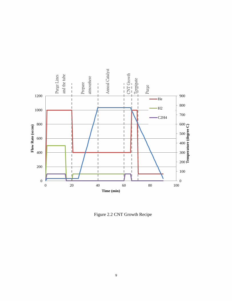
LabVIEW software. The complete recipe of flow rate and furnace temperature is shown in

Figure 2.2.

Before each growth, a prebaking process is carried out to clean the tube and lower the

humidity in the tube. The prebaking happens at 950 for 50 minutes. After prebaking,

each sample is loaded manually into the tube at 60 mm from the end of the tube. Figure

2.3 shows the schematic and the actual set-up of the experiment. The sample is loaded at

such a location because the growth rate is observed to be the best at this location (also

known as “sweet spot”) [16].

9

Figure 2.2 CNT Growth Recipe

0

100

200

300

400

500

600

700

800

900

0

200

400

600

800

1000

1200

0 20 40 60 80 100T

emp

era

ture

(d

egre

e C

)

Flo

w R

ate

(sc

cm)

Time (min)

He

H2

C2H4

Pur

ge L

ines

and

the

tube

Pre

pare

atm

osph

ere

Ann

eal

Cat

alys

t

CN

T G

row

th

Ter

min

ate

Pur

ge

10

Figure 2.3 Tube Furnace for CNT Growth (a) Schematics (b) Actual set-up

Furnace Mineral Oil Bubbler

Exhaust

Sample

He

H2

C2H4

Dry

Air

Furnace

DAQ PC

Exhaust

Quartz Tube

Mineral Oil Bubbler Sample

(b)

(a)

11

Followed by prebaking is the actual growth of CNT. First, the tube is purged with all

gases for 15 minutes. This step purges the tube and decreases the humidity of the tube. The

catalyst is then annealed for 20 minutes at 775. Followed by annealing is the actual

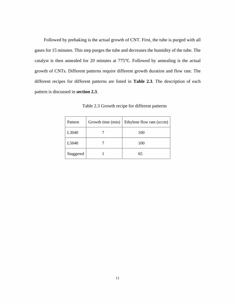
growth of CNTs. Different patterns require different growth duration and flow rate. The

different recipes for different patterns are listed in Table 2.3. The description of each

pattern is discussed in section 2.3.

Table 2.3 Growth recipe for different patterns

Pattern Growth time (min) Ethylene flow rate (sccm)

L3040 7 100

L5040 7 100

Staggered 1 65

12

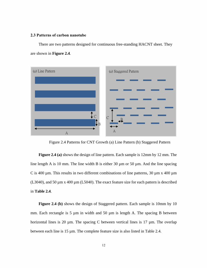
2.3 Patterns of carbon nanotube

There are two patterns designed for continuous free-standing HACNT sheet. They

are shown in Figure 2.4.

Figure 2.4 Patterns for CNT Growth (a) Line Pattern (b) Staggered Pattern

Figure 2.4 (a) shows the design of line pattern. Each sample is 12mm by 12 mm. The

line length A is 10 mm. The line width B is either 30 µm or 50 µm. And the line spacing

C is 400 µm. This results in two different combinations of line patterns, 30 µm x 400 µm

(L3040), and 50 µm x 400 µm (L5040). The exact feature size for each pattern is described

in Table 2.4.

Figure 2.4 (b) shows the design of Staggered pattern. Each sample is 10mm by 10

mm. Each rectangle is 5 µm in width and 50 µm is length A. The spacing B between

horizontal lines is 20 µm. The spacing C between vertical lines is 17 µm. The overlap

between each line is 15 µm. The complete feature size is also listed in Table 2.4.

(a) Line Pattern (a) Staggered Pattern

A

B

C

A

B C

13

Table 2.4 Feature size of each pattern

Line A(µm) B (µm) C(µm)

L3040 10000 30 400

L5040 10000 50 400

Staggered 50 20 17

The line patterns are designed such that the overlap between each individual CNT

feature is increased along one direction. The Staggered patterns are designed to further

increase the overlap between each individual CNT pattern.

The line pattern results in overlap across the length of each feature, whereas the

Staggered pattern results in overlap across both the length and the width of each feature.

The design of these increased overlap is aiming at increase the shear stress between each

feature, which in turn increases the mechanical strength and conductivity of each free-

standing CNT sheet.

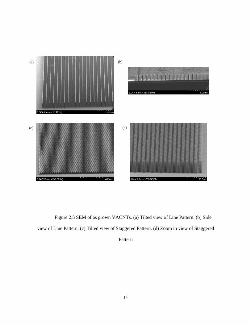
Figure 2.5 shows the SEM images of as grown VACNTs for both patterns. It can be

seen from these SEM images that the growth is fairly straight.

14

Figure 2.5 SEM of as grown VACNTs. (a) Tilted view of Line Pattern. (b) Side

view of Line Pattern. (c) Tilted view of Staggered Pattern. (d) Zoom in view of Staggered

Pattern

(a) (b)

(c) (d)

15

2.4 Transfer of structured carbon nanotube

After each growth of structured CNTs, the height is recorded using SEM. Each sample

is then transferred to another polymer transfer substrate. This substrate serves as a carrier

film so that structured CNTs can be assembled horizontally and a free-standing sheet can

be achieved.

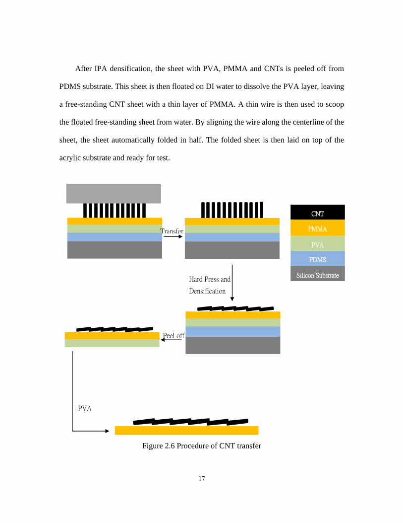
Figure 2.6 shows the schematic of a transfer substrate and the process of transfer.

Each transfer substrate consists of a layer of polydimethylsiloxane (PDMS), polyvinyl

alcohol (PVA), and poly (methyl methacrylate) (PMMA) from bottom to top, which lies

on top of a silicon substrate. PDMS layer serves as a media to delaminate PVA from silicon

substrate. PVA is a sacrificial layer which will later be dissolved in water. PMMA is the

adhesion layer to promote adhesion between CNTs and the transfer substrate.

The recipe for making each layer of polymer is listed in Table 2.5. The weight ratio

of silicon elastomer curing agent to silicon elastomer base is 1:10. After stirring and mixing

for 5 minutes, the solution is held under vacuum for 20 minutes to get rid of the air bubbles.

The mixed PDMS solution is then poured on top of a silicon wafer, and spin coat for 5

minutes at 5000 rpm. After that, the wafer is cured at 40 for 2 hours. The thickness of

PDMS layer is typically 3 µm to 5 µm. The silicon wafer is then cut into small sizes to

accommodate the size of each CNT sample.

16

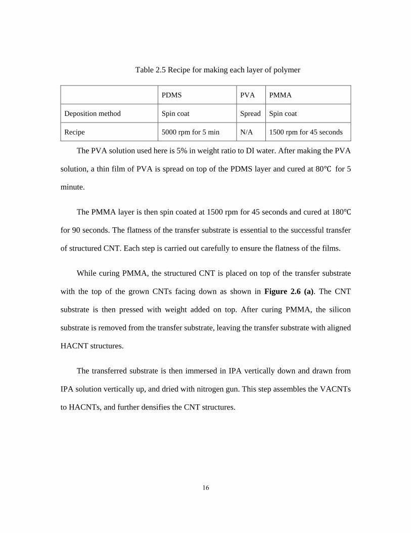
Table 2.5 Recipe for making each layer of polymer

PDMS PVA PMMA

Deposition method Spin coat Spread Spin coat

Recipe 5000 rpm for 5 min N/A 1500 rpm for 45 seconds

The PVA solution used here is 5% in weight ratio to DI water. After making the PVA

solution, a thin film of PVA is spread on top of the PDMS layer and cured at 80 for 5

minute.

The PMMA layer is then spin coated at 1500 rpm for 45 seconds and cured at 180

for 90 seconds. The flatness of the transfer substrate is essential to the successful transfer

of structured CNT. Each step is carried out carefully to ensure the flatness of the films.

While curing PMMA, the structured CNT is placed on top of the transfer substrate

with the top of the grown CNTs facing down as shown in Figure 2.6 (a). The CNT

substrate is then pressed with weight added on top. After curing PMMA, the silicon

substrate is removed from the transfer substrate, leaving the transfer substrate with aligned

HACNT structures.

The transferred substrate is then immersed in IPA vertically down and drawn from

IPA solution vertically up, and dried with nitrogen gun. This step assembles the VACNTs

to HACNTs, and further densifies the CNT structures.

17

After IPA densification, the sheet with PVA, PMMA and CNTs is peeled off from

PDMS substrate. This sheet is then floated on DI water to dissolve the PVA layer, leaving

a free-standing CNT sheet with a thin layer of PMMA. A thin wire is then used to scoop

the floated free-standing sheet from water. By aligning the wire along the centerline of the

sheet, the sheet automatically folded in half. The folded sheet is then laid on top of the

acrylic substrate and ready for test.

Figure 2.6 Procedure of CNT transfer

Transfer

Hard Press and

Densification

Peel off

PVA

PDMS

PVA

PMMA

Silicon Substrate

CNT

18

Figure 2.7 shows the floated sheet, and the schematics of picking up the sheet from

water.

Figure 2.7 Schematic of preparing for test (a) Schematic of free-standing sheet

floating on water, (b) Schematic of picking the sheet up from water with thin wire, (c)

Optical image of free-standing sheet floating on water, (d) Schematic of placing free-

standing sheet on acrylic parts and pulling the thin wire and (e) Schematic of prepared

free-standing sheet on acrylic parts

(a) (b) (c)

(d) (e)

19

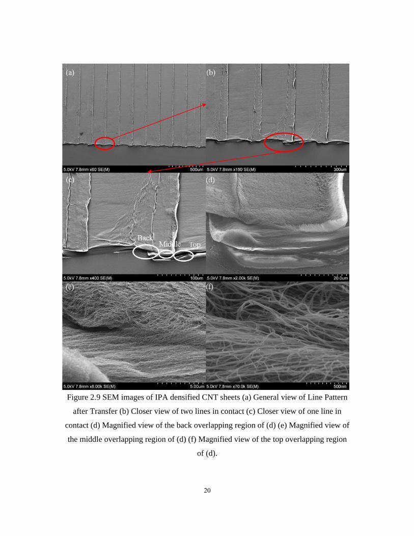
Figure 2.8 shows SEM images of transferred CNT sheets for line patterns. Figure 2.9

shows SEM images of the same sheet after IPA densification. It is observed that IPA

densification improves the contact between overlap CNT features.

Figure 2.8 SEM images of transferred CNT sheets (a) General view of Line Pattern after

Transfer (b) Closer view of two lines in contact (c) Closer view of one line in contact (d)

Magnified view of the back overlapping region of (d) (e) Magnified view of the middle

overlapping region of (d) (f) Magnified view of the top overlapping region of (d).

20

Figure 2.9 SEM images of IPA densified CNT sheets (a) General view of Line Pattern

after Transfer (b) Closer view of two lines in contact (c) Closer view of one line in

contact (d) Magnified view of the back overlapping region of (d) (e) Magnified view of

the middle overlapping region of (d) (f) Magnified view of the top overlapping region

of (d).

21

2.5 Electrical Test preparation

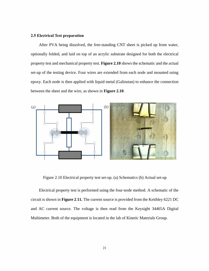
After PVA being dissolved, the free-standing CNT sheet is picked up from water,

optionally folded, and laid on top of an acrylic substrate designed for both the electrical

property test and mechanical property test. Figure 2.10 shows the schematic and the actual

set-up of the testing device. Four wires are extended from each node and mounted using

epoxy. Each node is then applied with liquid metal (Galinstan) to enhance the connection

between the sheet and the wire, as shown in Figure 2.10.

Figure 2.10 Electrical property test set-up. (a) Schematics (b) Actual set-up

Electrical property test is performed using the four-node method. A schematic of the

circuit is shown in Figure 2.11. The current source is provided from the Keithley 6221 DC

and AC current source. The voltage is then read from the Keysight 34465A Digital

Multimeter. Both of the equipment is located in the lab of Kinetic Materials Group.

(a) (b)

22

Figure 2.11 Schematic of the circuit for electrical property test

The current is applied from -2.5 mA to +2.5 mA with a 0.5 mA increment and

excluding 0.0 mA. After reading the voltage at each current input, an IV-curve is obtained,

where the resistance is the slope of the curve. The conductivity is then calculated based on

the following equation

𝑆 =𝐿

𝑅𝐴 2.1

where R is the resistance of the sample, L is the length between two inner nodes, and A is

the cross-sectional area of each sample. The cross-sectional area of each sample is

calculated based on the thickness and width of each sample. The thickness is characterized

in section 4.1. Both length and width are measured manually each time before the test.

For each pattern, eight experiments at different growth height are performed, where

within each growth height; two separate experiments on the same growth height are

performed. Thus, a total of 80 experiments are performed. All the results are shown and

discussed in Chapter 4.

V

A

23

2.6 Mechanical Test preparation

After each electrical property test, a mechanical property test is followed. The device

is mounted on a tensile test station by epoxy. After the epoxy cured, the clippers are taken

off, and a tensile test is followed.

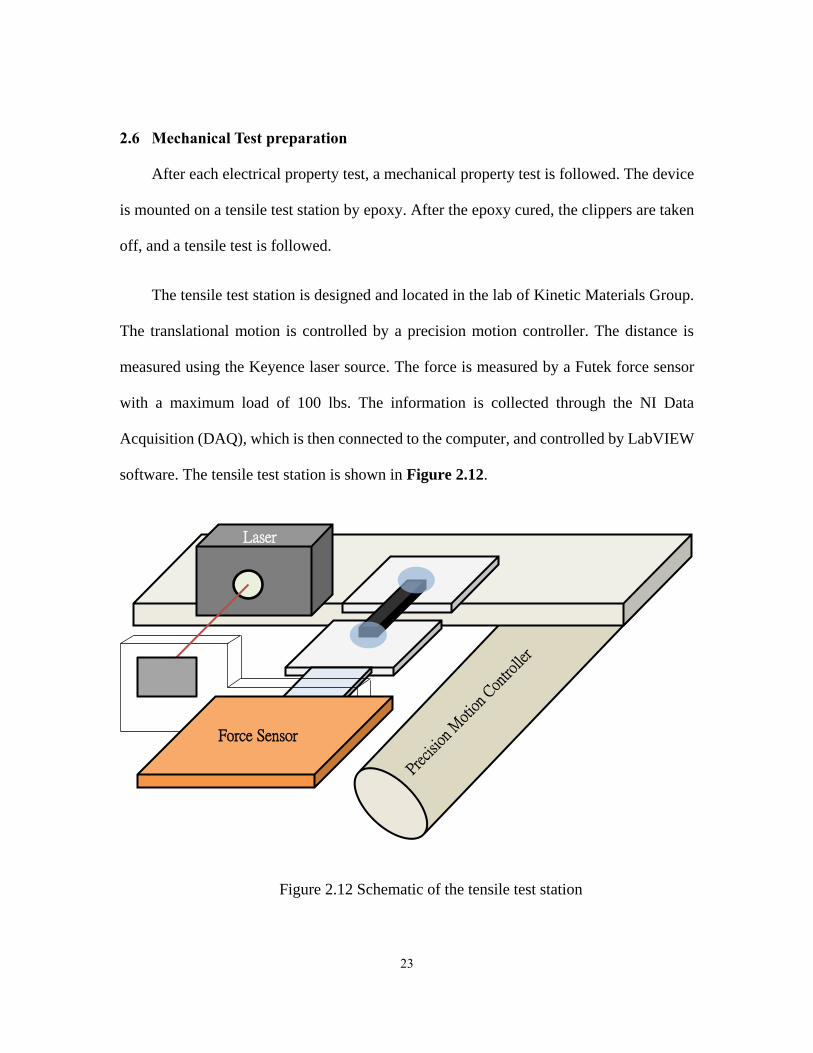
The tensile test station is designed and located in the lab of Kinetic Materials Group.

The translational motion is controlled by a precision motion controller. The distance is

measured using the Keyence laser source. The force is measured by a Futek force sensor

with a maximum load of 100 lbs. The information is collected through the NI Data

Acquisition (DAQ), which is then connected to the computer, and controlled by LabVIEW

software. The tensile test station is shown in Figure 2.12.

Figure 2.12 Schematic of the tensile test station

Force Sensor

Laser

24

Figure 2.13 Actual experimental set-up of the tensile test station

Figure 2.13 shows the actual experimental set-up of the tensile test station. From the

LabVIEW software, the acceleration and velocity of the motion controller can be set up

prior to each experiment. The values that are used for our experiments are 0.005 mm/s for

velocity and 0.5mm/s2 for acceleration. After setting up the velocity and acceleration, the

test can be recorded and started by giving a known displacement. The same as electrical

property test, a total of 80 experiments are performed.

Laser

Force Sensor

25

CHAPTER 3 CAPILLARY FORCE MODELING

Capillary force acts between CNTs when liquid is present. The capillary force shrinks

CNTs to a smaller size compared to before densification. This chapter discusses the main

approach that is used to model the capillary force between CNTs due to densification to

help better understand the densification step of our free-standing CNT sheets.

3.1 Capillary force between carbon nanotubes

It has been observed that CNTs can self-assemble when densified in liquid [16].

Section 2.4 discusses the steps for IPA densification. CNTs are dipped in IPA vertically,

and slowly drawn from IPA. The sheet is then dried with nitrogen blowing from top of the

sheet to bottom to enhance self-assembly.

When dipped in IPA, the strong van der Waals interactions “zip” the CNTs together

and densely pack CNTs [17]. The CNTs then self-assemble due to the presence of capillary

force [18]. The densification and drawing direction affects the self-assembly direction.

The effect of capillary force from liquid densification has been well studied [16] [17]

[18]. However, the full mechanism of capillary force has not been well-understood. In the

following sections, modeling of capillary forces between CNTs is carried out to further

understand mechanisms of capillary forces between CNTs.

26

3.2 Capillary force modeling using finite element analysis

I use Finite Element Analysis (FEA) based on self-derived MATLAB code to model

capillary forces between CNTs. The complete code is attached in the appendix.

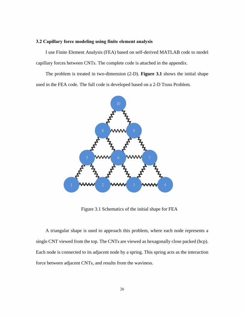
The problem is treated in two-dimension (2-D). Figure 3.1 shows the initial shape

used in the FEA code. The full code is developed based on a 2-D Truss Problem.

Figure 3.1 Schematics of the initial shape for FEA

A triangular shape is used to approach this problem, where each node represents a

single CNT viewed from the top. The CNTs are viewed as hexagonally close packed (hcp).

Each node is connected to its adjacent node by a spring. This spring acts as the interaction

force between adjacent CNTs, and results from the waviness.

10

1 4

8 9

5 6 7

2 3

27

Each node is also connected to the ground by two springs. These springs act as the

bound between each individual CNT to the substrate. Due to the typically long aspect ratio

of CNTs, each 2D cross section is under the effect of substrate effect rising from the cross

section below and above it. This allows me to treat the 3D behavior of CNTs as a 2D

problem. Figure 3.2 shows the schematic of the grounded node.

Figure 3.2 Schematic of a grounded node where springs represent substrate effect

on the CNT in the out of plane direction, and the node represents an individual CNT

The spring stiffness assumes the value of 106 GPa for both of the ground springs. With

these two grounded node, each individual CNT is able to move freely, but are forced to

return to its original position if the applied force is removed. In addition, the movement of

the node is symmetrical with respect to the direction of the applied force.

The FEA code developed here combined both the spring interaction between each

node, and the two grounded nodes on each individual CNT. The full algorithm of capillary

force modeling, including the boundary conditions and matrices is discussed in the

following section.

28

3.3 Algorithm of modeling

In order to use FEA, equations and boundary conditions are derived. The basic

equation to calculate displacement of the node is

[𝐾][𝑈] = [𝐹] 3.1

where [𝐾] is the global stiffness matrix, [𝑈] is the global displacement matrix, and [𝐹]

is the global force matrix. The viscoelasticity of the CNT is ignored. F represents the

capillary forces causing the CNTs to zip together. This equation is derived based on

Hooke’s Law but applied to a system of matrices.

The difference between 1-D and 2-D problem in FEA is that, in 2-D, the stiffness

value for each element is calculated in its local coordinate, which is then transformed to

the global coordinate based on the angle of the element with respect to the ground.

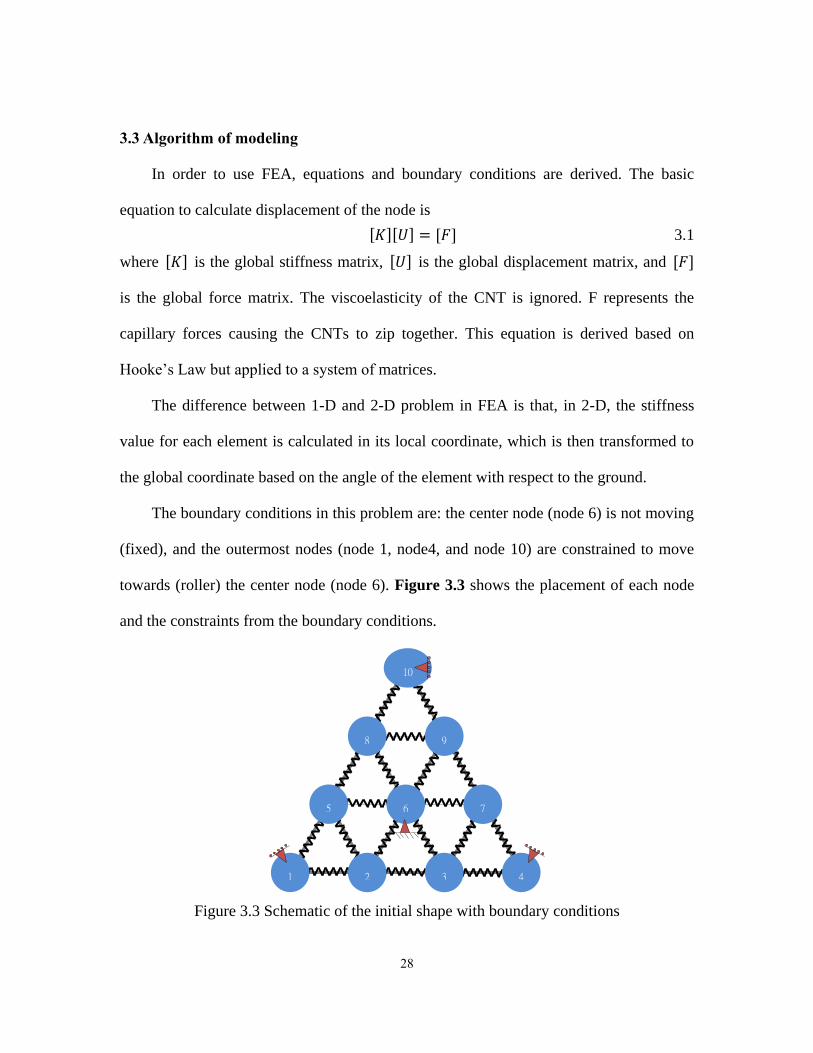
The boundary conditions in this problem are: the center node (node 6) is not moving

(fixed), and the outermost nodes (node 1, node4, and node 10) are constrained to move

towards (roller) the center node (node 6). Figure 3.3 shows the placement of each node

and the constraints from the boundary conditions.

Figure 3.3 Schematic of the initial shape with boundary conditions

10

1 4

8 9

5 6 7

2 3

29

The full algorithm includes set up the initial conditions, set up the equations to solve,

solve the equations, and post-processing calculations. Figure 3.4 shows the flow chart of

the code.

Figure 3.4 Flow chart of the code

CNT FEA (Main Code)

Read Input

Initialize Equation Module

Solve Module

Post Processing

Displacement Assemble Module

Stiffness Assemble Module

Force Assemble Module

Inclined Support Assemble Module

Assemble

Module

30

The Read Input file contains all of the initial conditions and values for this problem,

where it reads number of node, number of elements, number of load, number of prescribed

displacement (boundary conditions), the node where force is applied, the force value at

each node, the node where prescribed displacement is applied, the displacement value at

each node, and the original coordinate of each node. Figure 3.5 and Table 3.1 shows the

numbering of element and node in this code.

Figure 3.5 Element number and Node number

The main code contains everything else, as shown in Figure 3.4, where Initialize

Equation Module is set up from Read Input file, Assembly Modules (Displacement

Assemble, Force Assemble, Stiffness Assemble, and Inclined Support Assemble) assemble

and sort data at each node based on the Initialize Equation Module, Solve Module solves

10

1 4

8 9

5 6 7

2 3 A B C

D E F G H I

J K

L M N O

P

Q R

31

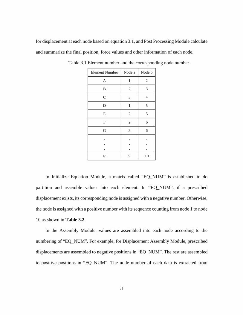
for displacement at each node based on equation 3.1, and Post Processing Module calculate

and summarize the final position, force values and other information of each node.

Table 3.1 Element number and the corresponding node number

Element Number Node a Node b

A 1 2

B 2 3

C 3 4

D 1 5

E 2 5

F 2 6

G 3 6

.

.

.

.

.

.

Q

.

.

.

8

.

.

.

10 R 9 10

In Initialize Equation Module, a matrix called “EQ_NUM” is established to do

partition and assemble values into each element. In “EQ_NUM”, if a prescribed

displacement exists, its corresponding node is assigned with a negative number. Otherwise,

the node is assigned with a positive number with its sequence counting from node 1 to node

10 as shown in Table 3.2.

In the Assembly Module, values are assembled into each node according to the

numbering of “EQ_NUM”. For example, for Displacement Assembly Module, prescribed

displacements are assembled to negative positions in “EQ_NUM”. The rest are assembled

to positive positions in “EQ_NUM”. The node number of each data is extracted from

32

“DISP_NODE” matrix, and the value at each node is extracted from “DISP_VAL” matrix.

The same applies to all other assembly modules.

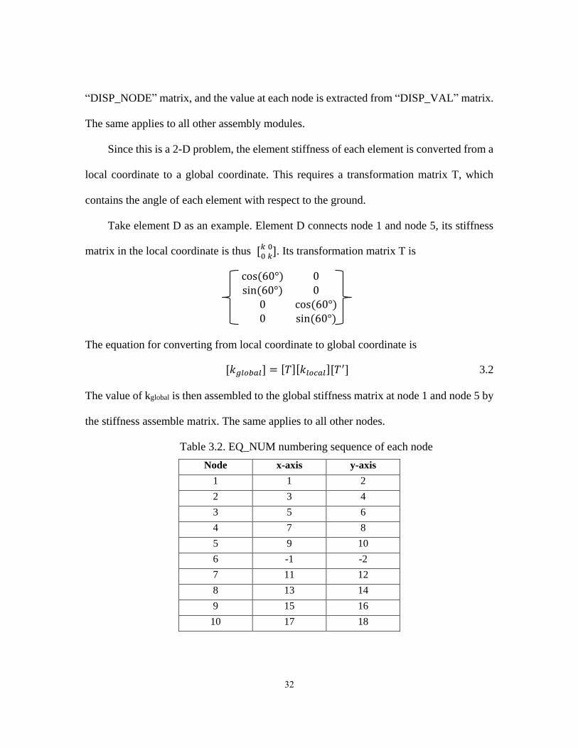
Since this is a 2-D problem, the element stiffness of each element is converted from a

local coordinate to a global coordinate. This requires a transformation matrix T, which

contains the angle of each element with respect to the ground.

Take element D as an example. Element D connects node 1 and node 5, its stiffness

matrix in the local coordinate is thus [𝑘00𝑘]. Its transformation matrix T is

cos(60°) 0sin(60°) 0

0 cos(60°)0 sin(60°)

The equation for converting from local coordinate to global coordinate is

[𝑘𝑔𝑙𝑜𝑏𝑎𝑙] = [𝑇][𝑘𝑙𝑜𝑐𝑎𝑙][𝑇′] 3.2

The value of kglobal is then assembled to the global stiffness matrix at node 1 and node 5 by

the stiffness assemble matrix. The same applies to all other nodes.

Table 3.2. EQ_NUM numbering sequence of each node

Node x-axis y-axis

1 1 2

2 3 4

3 5 6

4 7 8

5 9 10

6 -1 -2

7 11 12

8 13 14

9 15 16

10 17 18

33

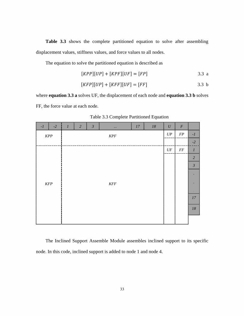
Table 3.3 shows the complete partitioned equation to solve after assembling

displacement values, stiffness values, and force values to all nodes.

The equation to solve the partitioned equation is described as

[𝐾𝑃𝑃][𝑈𝑃] + [𝐾𝑃𝐹][𝑈𝐹] = [𝐹𝑃] 3.3 a

[𝐾𝐹𝑃][𝑈𝑃] + [𝐾𝐹𝐹][𝑈𝐹] = [𝐹𝐹] 3.3 b

where equation 3.3 a solves UF, the displacement of each node and equation 3.3 b solves

FF, the force value at each node.

Table 3.3 Complete Partitioned Equation

-1 -2 1 2 3 … 17 18 U F

KPP KPF UP FP -1

-2

KFP KFF

UF FF 1

2

3

.

.

.

17

18

The Inclined Support Assemble Module assembles inclined support to its specific

node. In this code, inclined support is added to node 1 and node 4.

34

Section 3.4 further discusses the code for modeling capillary force acting against

CNTs. Whereas section 3.5 further discuss the code for modeling capillary force acting

along the outline of CNTs.

3.4 Capillary force acting against carbon nanotubes

Figure 3.6 shows the boundary conditions for modeling capillary force acting against

CNTs and the hexagonally close packed configuration.

Figure 3.6 Boundary conditions for capillary force acting against CNTs

10

1 4

8 9

5 6 7

2 3

35

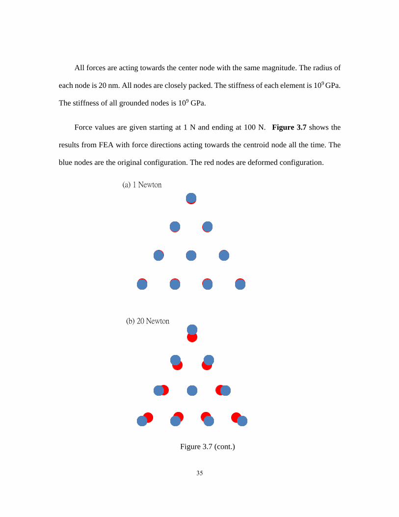
All forces are acting towards the center node with the same magnitude. The radius of

each node is 20 nm. All nodes are closely packed. The stiffness of each element is 109 GPa.

The stiffness of all grounded nodes is 109 GPa.

Force values are given starting at 1 N and ending at 100 N. Figure 3.7 shows the

results from FEA with force directions acting towards the centroid node all the time. The

blue nodes are the original configuration. The red nodes are deformed configuration.

Figure 3.7 (cont.)

(a) 1 Newton

(b) 20 Newton

36

Figure 3.7 (cont.)

(c) 40 Newton

(d) 60 Newton

37

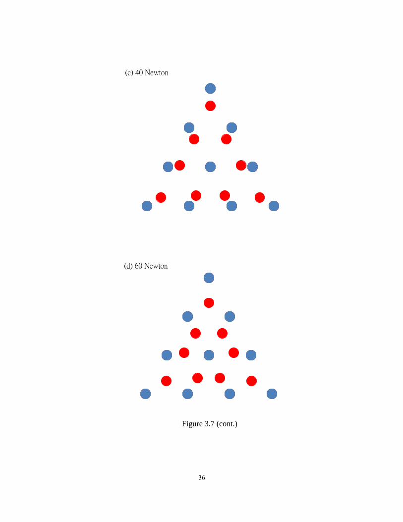
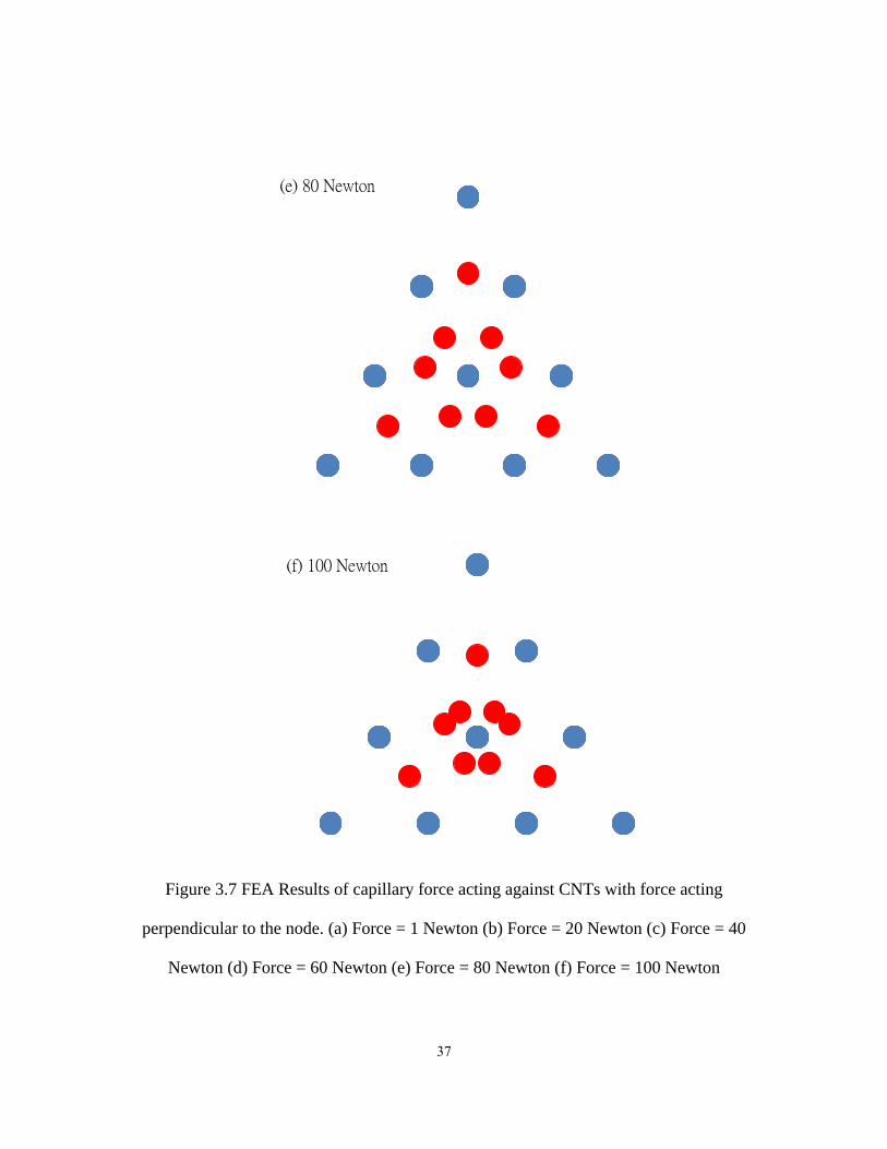
Figure 3.7 FEA Results of capillary force acting against CNTs with force acting

perpendicular to the node. (a) Force = 1 Newton (b) Force = 20 Newton (c) Force = 40

Newton (d) Force = 60 Newton (e) Force = 80 Newton (f) Force = 100 Newton

(e) 80 Newton

(f) 100 Newton

38

From the results shown in Figure 3.7, it is observed that, as capillary forces are acting

against CNTs, the CNTs shrink in size but remain its original shape. The effect of capillary

force shrinks the sample in size but not in shape.

3.5 Capillary force acting along the outline of carbon nanotubes

Figure 3.8 shows the boundary conditions of capillary force acting along the outline

of CNTs.

Figure 3.8 Boundary conditions of capillary force acting along CNTs

10

1 4

8 9

5 6 7

2 3

39

All spring elements along the outline of CNTs are in tension. The center node (node

6) is fixed. The outermost nodes (node 1, node 4, and node 10) are restricted to move

towards the center node. The stiffness of element spring is 109 GPa. The stiffness of all

grounded nodes is 106 GPa. The force values start at 1 N and end at 30 N. Figure 3.9 shows

the results from FEA.

Figure 3.8 (cont.)

(a) 10 Newton

(b) 20 Newton

40

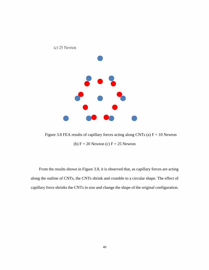
Figure 3.8 FEA results of capillary forces acting along CNTs (a) F = 10 Newton

(b) F = 20 Newton (c) F = 25 Newton

From the results shown in Figure 3.8, it is observed that, as capillary forces are acting

along the outline of CNTs, the CNTs shrink and crumble to a circular shape. The effect of

capillary force shrinks the CNTs in size and change the shape of the original configuration.

(c) 25 Newton

41

3.6 Discussion of FEA modeling of capillary forces

Comparing Figure 3.7 (c) and Figure 3.8 (a), it is observed that, when the capillary

force is small, CNTs remain the original shape (triangular) despite the two different

mechanisms.

However, when the effect of capillary force increases, there is a big difference

between the two mechanisms. When capillary force acts against the outer nodes, the CNTs

shrink in size but remain its original shape. When capillary force acts along the outer nodes,

however, the CNTs shrink and crumble to a circular shape.

The results from FEA explains why these CNTs features shrinks in size and penetrate

into each other as it is densified in IPA. It is important to use capillary forces to further

densify CNTs sheets and enhance the penetration between overlapping regions to improve

its electrical and mechanical properties.

42

CHAPTER 4 RESULTS AND DISCUSSION

4.1 Thickness Characterization

In order to determine the properties of each sample, the cross-sectional area needs to

be determined, which requires the thickness of each pattern. Here I derived the average

thickness of each pattern based on the growth height H.

The area of each feature is calculated as growth height H times the feature length L.

The total area of each sample is the area of each feature (𝐻 × 𝐿) times the number of

features N. There are 31 features for both Line Patterns, and 130130 features for Staggered

Pattern. By dividing this area by the unit area of each sample, I derive the number of layer

of each sample. Unit area 𝐴0 for both Line Patterns is 12𝑚𝑚 × 12𝑚𝑚 = 144 𝑚𝑚2.

Unit Area for Staggered Pattern is 10𝑚𝑚 × 10𝑚𝑚 = 1002 The total average thickness

is then the number of layer times the unit thickness of each pattern, as described below

𝑇𝑜𝑡𝑎𝑙 𝐴𝑣𝑒𝑟𝑎𝑔𝑒 𝑇ℎ𝑖𝑐𝑘𝑛𝑒𝑠𝑠 = 𝑡𝑑 ×𝐻×𝐿×𝑁

𝐴0 4.1

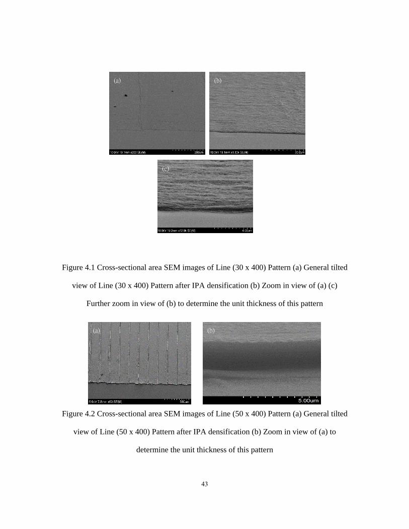
The thickness value 𝑡𝑑 of one layer of each pattern is determined using SEM.

Figure 4.1 shows the cross-sectional SEM images of line (30 x 400) pattern after IPA

densification. Figure 4.2 shows the same SEM images of line (50 x 400) pattern.

Figure 4.3 shows the SEM images of staggered pattern. It is observed that the thickness of

each pattern is largely reduced after transfer and IPA densification.

43

Figure 4.1 Cross-sectional area SEM images of Line (30 x 400) Pattern (a) General tilted

view of Line (30 x 400) Pattern after IPA densification (b) Zoom in view of (a) (c)

Further zoom in view of (b) to determine the unit thickness of this pattern

Figure 4.2 Cross-sectional area SEM images of Line (50 x 400) Pattern (a) General tilted

view of Line (50 x 400) Pattern after IPA densification (b) Zoom in view of (a) to

determine the unit thickness of this pattern

(a) (b)

(a) (b)

(c)

44

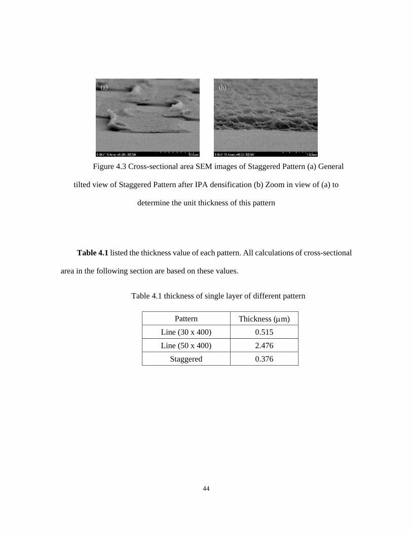
Figure 4.3 Cross-sectional area SEM images of Staggered Pattern (a) General

tilted view of Staggered Pattern after IPA densification (b) Zoom in view of (a) to

determine the unit thickness of this pattern

Table 4.1 listed the thickness value of each pattern. All calculations of cross-sectional

area in the following section are based on these values.

Table 4.1 thickness of single layer of different pattern

Pattern Thickness (m)

Line (30 x 400) 0.515

Line (50 x 400) 2.476

Staggered 0.376

(a) (b)

45

4.2 Electrical Conductivity

Electrical Conductivity of each sample is tested using the four-probe method, as

discussed in section 2.5. The resistance R is obtained from the slope of the I-V curve, the

conductivity 𝑆 is calculated based on the following equation

𝑆 = 𝐿

𝑅𝐴 4.2

where A is the cross-sectional area of each sample, and L is the distance between the two

inner nodes.

Each pattern is tested at 12 different growth height. At each growth height, 2 tests

from the same sample is conducted in parallel. The results of all tests for different patterns

are discussed in the following sections.

4.3 Mechanical Strength

Mechanical strength of each sample is tested using the tensile test station described in

section 2.6. The tensile test station reads the force-displacement curve. After obtaining the

force-displacement curve. The stress is calculated by dividing the cross-sectional area of

each sample from the force F. The equation is described below

𝜎 =𝐹

𝐴 4.3

The strength of each sample is then the maximum value from each set of data. All

mechanical strength tests are carried out after the electrical conductivity tests. Same as

electrical conductivity tests, each patterns in tested at 12 different growth height. At each

growth height, 2 tests are conducted in parallel. The results of these tests are discussed in

the following sections.

46

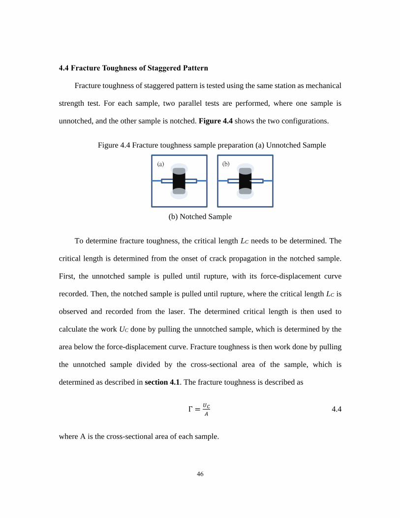
4.4 Fracture Toughness of Staggered Pattern

Fracture toughness of staggered pattern is tested using the same station as mechanical

strength test. For each sample, two parallel tests are performed, where one sample is

unnotched, and the other sample is notched. Figure 4.4 shows the two configurations.

Figure 4.4 Fracture toughness sample preparation (a) Unnotched Sample

(b) Notched Sample

To determine fracture toughness, the critical length LC needs to be determined. The

critical length is determined from the onset of crack propagation in the notched sample.

First, the unnotched sample is pulled until rupture, with its force-displacement curve

recorded. Then, the notched sample is pulled until rupture, where the critical length LC is

observed and recorded from the laser. The determined critical length is then used to

calculate the work UC done by pulling the unnotched sample, which is determined by the

area below the force-displacement curve. Fracture toughness is then work done by pulling

the unnotched sample divided by the cross-sectional area of the sample, which is

determined as described in section 4.1. The fracture toughness is described as

Γ =𝑈𝐶

𝐴 4.4

where A is the cross-sectional area of each sample.

(1

(a) (b)

47

4.5 Results of Line Pattern (30 x 400)

In total, 9 samples were tested, where 2 parallel tests are conducted for each sample.

The growth height of line (30 x 400) pattern is controlled between 450 µm to 850 µm.

Figure 4.5 I-V curve of the best results from Line (30 x 400) pattern

Figure 4.5 shows the I-V curve of the best results among these samples. The growth

height of this sample is 496 µm. According to equation 4.1, the thickness of the sample is

0.699 µm. The cross-sectional area of the sample is thus 0.00105 mm2. The length between

inner nodes is 6.5 mm. From the slope, the resistance of this sample is 80.26 Ω. Using

equation 4.2, the conductivity of this sample is 77.1 kS/m. Table 4.2 listed the data of this

sample.

y = 80.258x + 0.846

R² = 1

-250

-200

-150

-100

-50

0

50

100

150

200

250

-3 -2 -1 0 1 2 3

Vo

lta

ge

(mV

)

Current (mA)

48

Table 4.2. Data of the electrical conductivity result from the best sample of Line (30 x

400) Pattern

Conductivity (kS/m) 77.1

H (µm) 496

td (µm) 0.699

Length (mm) 6.50

Area (mm2) 0.00105

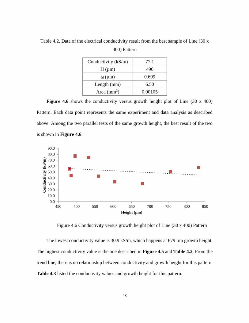
Figure 4.6 shows the conductivity versus growth height plot of Line (30 x 400)

Pattern. Each data point represents the same experiment and data analysis as described

above. Among the two parallel tests of the same growth height, the best result of the two

is shown in Figure 4.6.

Figure 4.6 Conductivity versus growth height plot of Line (30 x 400) Pattern

The lowest conductivity value is 30.9 kS/m, which happens at 679 µm growth height.

The highest conductivity value is the one described in Figure 4.5 and Table 4.2. From the

trend line, there is no relationship between conductivity and growth height for this pattern.

Table 4.3 listed the conductivity values and growth height for this pattern.

0.0

10.0

20.0

30.0

40.0

50.0

60.0

70.0

80.0

90.0

450 500 550 600 650 700 750 800 850

Co

nd

uct

ivit

y (

kS

/m)

Height (µm)

49

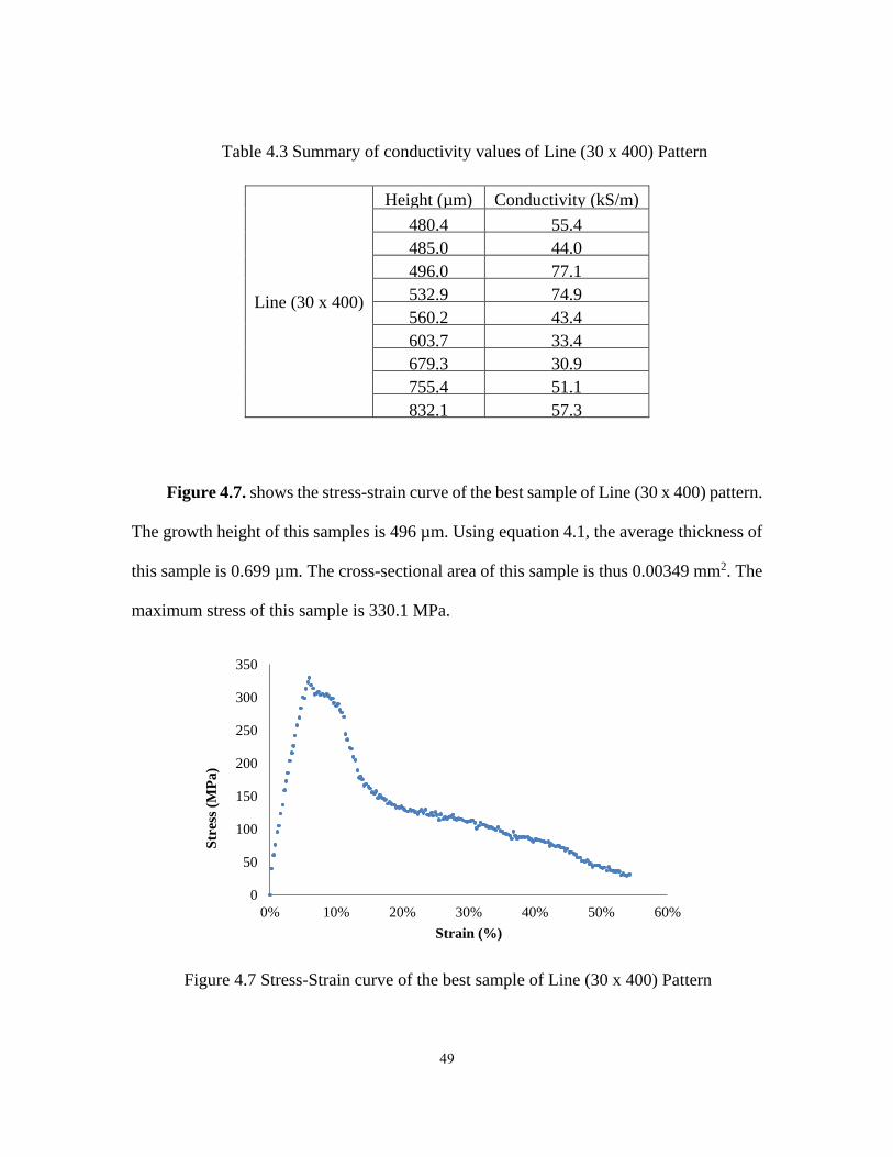
Table 4.3 Summary of conductivity values of Line (30 x 400) Pattern

Line (30 x 400)

Height (µm) Conductivity (kS/m)

480.4 55.4

485.0 44.0

496.0 77.1

532.9 74.9

560.2 43.4

603.7 33.4

679.3 30.9

755.4 51.1

832.1 57.3

Figure 4.7. shows the stress-strain curve of the best sample of Line (30 x 400) pattern.

The growth height of this samples is 496 µm. Using equation 4.1, the average thickness of

this sample is 0.699 µm. The cross-sectional area of this sample is thus 0.00349 mm2. The

maximum stress of this sample is 330.1 MPa.

Figure 4.7 Stress-Strain curve of the best sample of Line (30 x 400) Pattern

0

50

100

150

200

250

300

350

0% 10% 20% 30% 40% 50% 60%

Str

ess

(MP

a)

Strain (%)

50

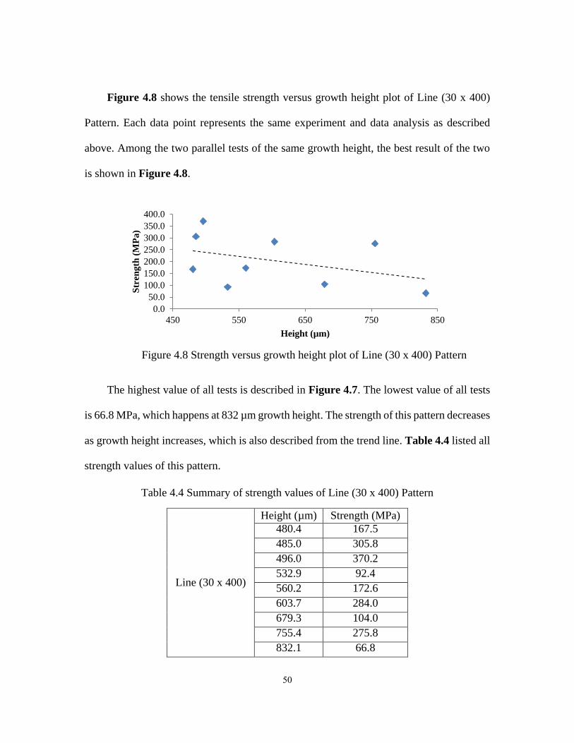
Figure 4.8 shows the tensile strength versus growth height plot of Line (30 x 400)




Figure 4.8 Strength versus growth height plot of Line (30 x 400) Pattern

The highest value of all tests is described in Figure 4.7. The lowest value of all tests

is 66.8 MPa, which happens at 832 µm growth height. The strength of this pattern decreases

as growth height increases, which is also described from the trend line. Table 4.4 listed all

strength values of this pattern.

Table 4.4 Summary of strength values of Line (30 x 400) Pattern

Line (30 x 400)

Height (µm) Strength (MPa)

480.4 167.5

485.0 305.8

496.0 370.2

532.9 92.4

560.2 172.6

603.7 284.0

679.3 104.0

755.4 275.8

832.1 66.8

0.0

50.0

100.0

150.0

200.0

250.0

300.0

350.0

400.0

450 550 650 750 850

Str

eng

th (

MP

a)

Height (µm)

51

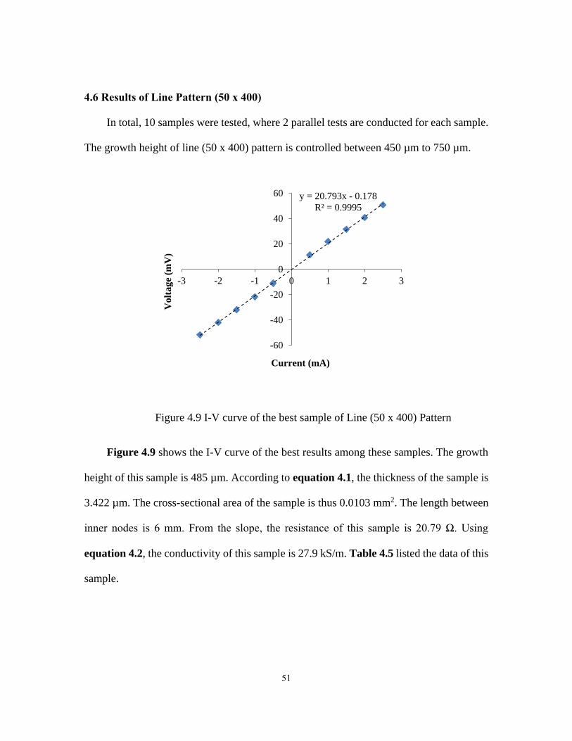
4.6 Results of Line Pattern (50 x 400)


The growth height of line (50 x 400) pattern is controlled between 450 µm to 750 µm.

Figure 4.9 I-V curve of the best sample of Line (50 x 400) Pattern



3.422 µm. The cross-sectional area of the sample is thus 0.0103 mm2. The length between

inner nodes is 6 mm. From the slope, the resistance of this sample is 20.79 Ω. Using

equation 4.2, the conductivity of this sample is 27.9 kS/m. Table 4.5 listed the data of this

sample.

y = 20.793x - 0.178

R² = 0.9995

-60

-40

-20

0

20

40

60

-3 -2 -1 0 1 2 3

Volt

age (

mV

)

Current (mA)

52

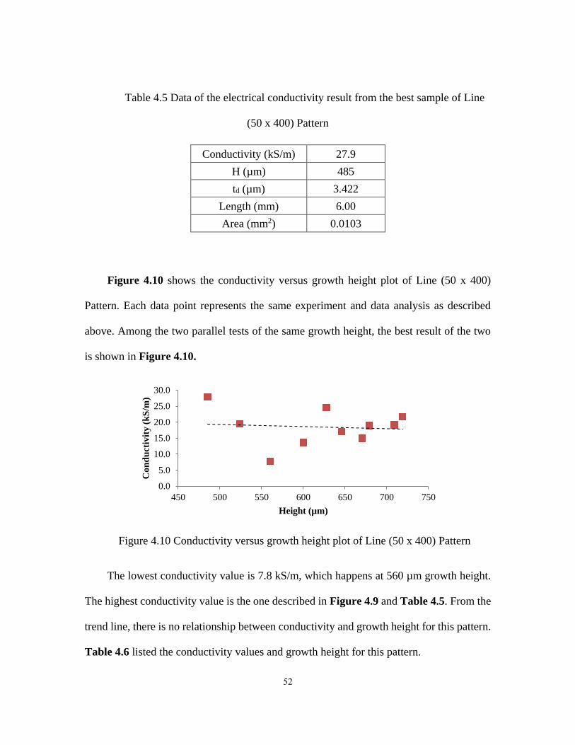
Table 4.5 Data of the electrical conductivity result from the best sample of Line

(50 x 400) Pattern


H (µm) 485

td (µm) 3.422

Length (mm) 6.00

Area (mm2) 0.0103

Figure 4.10 shows the conductivity versus growth height plot of Line (50 x 400)




Figure 4.10 Conductivity versus growth height plot of Line (50 x 400) Pattern


The highest conductivity value is the one described in Figure 4.9 and Table 4.5. From the

trend line, there is no relationship between conductivity and growth height for this pattern.

Table 4.6 listed the conductivity values and growth height for this pattern.

0.0

5.0

10.0

15.0

20.0

25.0

30.0

450 500 550 600 650 700 750

Co

nd

uct

ivit

y (

kS

/m)

Height (µm)

53

Table 4.6 Summary of conductivity values of Line (50 x 400) Pattern

Line (50 x 400)


485 27.9

524 19.4

560 7.8

600 13.6

628 24.6

646 17.0

670 14.9

679 18.9

709 19.1

719 21.7

Figure 4.11. shows the stress-strain curve of the best sample of Line (50 x 400) pattern.

The growth height of this samples is 719 µm. Using equation 4.1, the average thickness of

this sample is 4.917 µm. The cross-sectional area of this sample is thus 0.00492 mm2. The


Figure 4.11 Stress-Strain curve of the best sample of Line (50 x 400) Pattern

0

20

40

60

80

100

120

0% 10% 20% 30% 40% 50% 60% 70% 80%

Str

ess

(MP

a)

Strain (%)

54

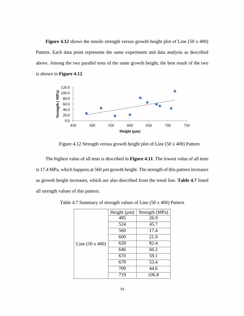
Figure 4.12 shows the tensile strength versus growth height plot of Line (50 x 400)




Figure 4.12 Strength versus growth height plot of Line (50 x 400) Pattern


is 17.4 MPa, which happens at 560 µm growth height. The strength of this pattern increases

as growth height increases, which are also described from the trend line. Table 4.7 listed

all strength values of this pattern.

Table 4.7 Summary of strength values of Line (50 x 400) Pattern

Line (50 x 400)

Height (µm) Strength (MPa)

485 26.9

524 45.7

560 17.4

600 21.9

628 82.4

646 66.2

670 59.1

679 53.4

709 44.6

719 106.8

0.0

20.0

40.0

60.0

80.0

100.0

120.0

450 500 550 600 650 700 750

Str

eng

th (

MP

a)

Height (µm)

55

4.7 Results of Staggered Pattern


Within the 12 samples, 5 samples are tested of fracture toughness. The growth height of

staggered pattern is controlled between 20 µm to 70 µm.

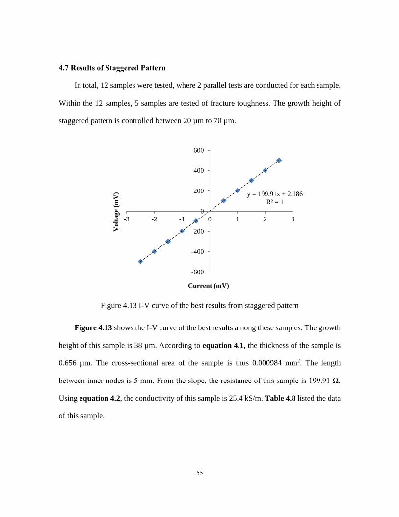
Figure 4.13 I-V curve of the best results from staggered pattern



0.656 µm. The cross-sectional area of the sample is thus 0.000984 mm2. The length

between inner nodes is 5 mm. From the slope, the resistance of this sample is 199.91 Ω.

Using equation 4.2, the conductivity of this sample is 25.4 kS/m. Table 4.8 listed the data

of this sample.

y = 199.91x + 2.186

R² = 1

-600

-400

-200

0

200

400

600

-3 -2 -1 0 1 2 3

Volt

age (

mV

)

Current (mV)

56

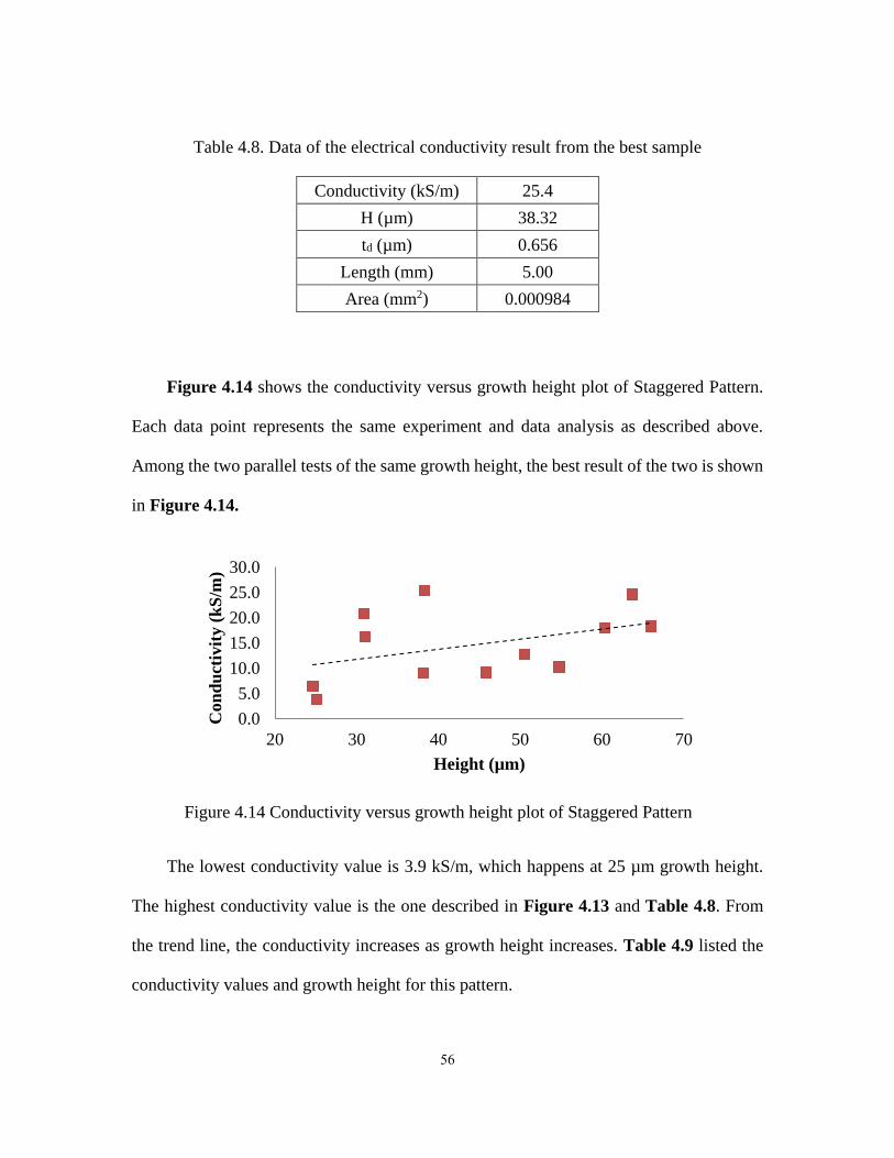
Table 4.8. Data of the electrical conductivity result from the best sample


H (µm) 38.32

td (µm) 0.656

Length (mm) 5.00

Area (mm2) 0.000984

Figure 4.14 shows the conductivity versus growth height plot of Staggered Pattern.

Each data point represents the same experiment and data analysis as described above.

Among the two parallel tests of the same growth height, the best result of the two is shown

in Figure 4.14.

Figure 4.14 Conductivity versus growth height plot of Staggered Pattern


The highest conductivity value is the one described in Figure 4.13 and Table 4.8. From

the trend line, the conductivity increases as growth height increases. Table 4.9 listed the

conductivity values and growth height for this pattern.

0.0

5.0

10.0

15.0

20.0

25.0

30.0

20 30 40 50 60 70

Con

du

ctiv

ity (

kS

/m)

Height (µm)

57

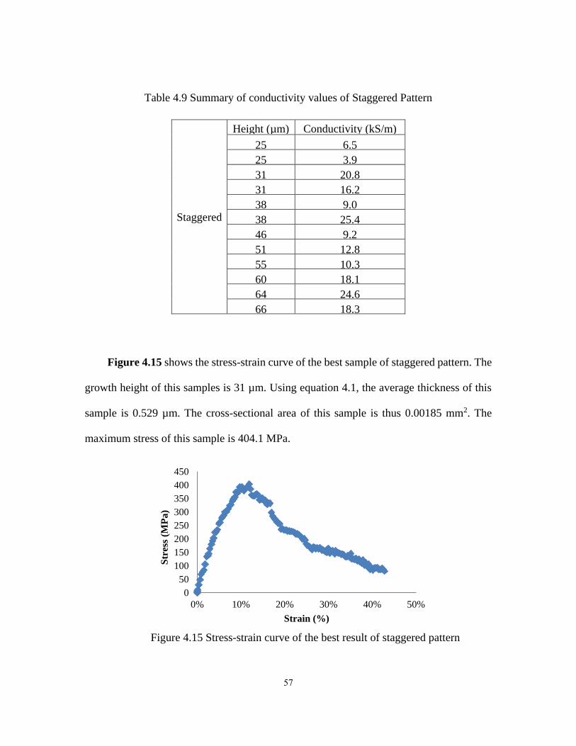
Table 4.9 Summary of conductivity values of Staggered Pattern

Staggered


25 6.5

25 3.9

31 20.8

31 16.2

38 9.0

38 25.4

46 9.2

51 12.8

55 10.3

60 18.1

64 24.6

66 18.3

Figure 4.15 shows the stress-strain curve of the best sample of staggered pattern. The

growth height of this samples is 31 µm. Using equation 4.1, the average thickness of this

sample is 0.529 µm. The cross-sectional area of this sample is thus 0.00185 mm2. The


Figure 4.15 Stress-strain curve of the best result of staggered pattern

0

50

100

150

200

250

300

350

400

450

0% 10% 20% 30% 40% 50%

Str

ess

(MP

a)

Strain (%)

58

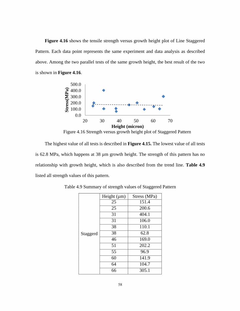
Figure 4.16 shows the tensile strength versus growth height plot of Line Staggered




Figure 4.16 Strength versus growth height plot of Staggered Pattern


is 62.8 MPa, which happens at 38 µm growth height. The strength of this pattern has no

relationship with growth height, which is also described from the trend line. Table 4.9

listed all strength values of this pattern.

Table 4.9 Summary of strength values of Staggered Pattern

Staggerd

Height (µm) Stress (MPa)

25 151.4

25 200.6

31 404.1

31 106.0

38 110.1

38 62.8

46 169.0

51 202.2

55 96.9

60 141.9

64 104.7

66 305.1

0.0

100.0

200.0

300.0

400.0

500.0

20 30 40 50 60 70

Str

ess(

MP

a)

Height (micron)

59

Figure 4.17 shows the fracture toughness test of the best sample of staggered pattern.

Figure 4.18 shows the parallel test with a pre-cut crack as described in section 4.4. The

growth height of this sample is 38 µm. Using equation 4.1, the average thickness of this

sample is 0.653 µm. The cross-sectional area of this sample is thus 0.00196 mm2. The

critical length LC is observed to be 0.23 mm. From Figure 4.17, the area under the curve

is 0.01098 N mm. Using equation 4.4, the fracture toughness of this sample is 5.6 kJ/m2.

Figure 4.17 Fracture toughness test of best sample of Staggered pattern without notch

Figure 4.18 Fracture toughness test of best sample of Staggered pattern with notch

0

0.05

0.1

0.15

0.2

0.25

0 0.2 0.4 0.6 0.8 1 1.2

Forc

e (N

)

Displacement (mm)

0

0.05

0.1

0.15

0 0.2 0.4 0.6 0.8 1 1.2

Forc

e (N

)

Displacement (mm)

60

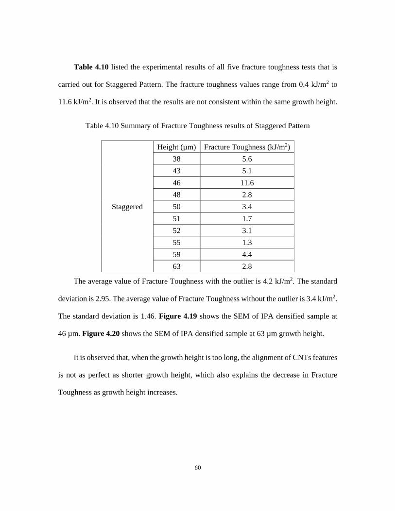
Table 4.10 listed the experimental results of all five fracture toughness tests that is

carried out for Staggered Pattern. The fracture toughness values range from 0.4 kJ/m2 to

11.6 kJ/m2. It is observed that the results are not consistent within the same growth height.

Table 4.10 Summary of Fracture Toughness results of Staggered Pattern

Staggered

Height (µm) Fracture Toughness (kJ/m2)

38 5.6

43 5.1

46 11.6

48 2.8

50 3.4

51 1.7

52 3.1

55 1.3

59 4.4

63 2.8

The average value of Fracture Toughness with the outlier is 4.2 kJ/m2. The standard

deviation is 2.95. The average value of Fracture Toughness without the outlier is 3.4 kJ/m2.

The standard deviation is 1.46. Figure 4.19 shows the SEM of IPA densified sample at

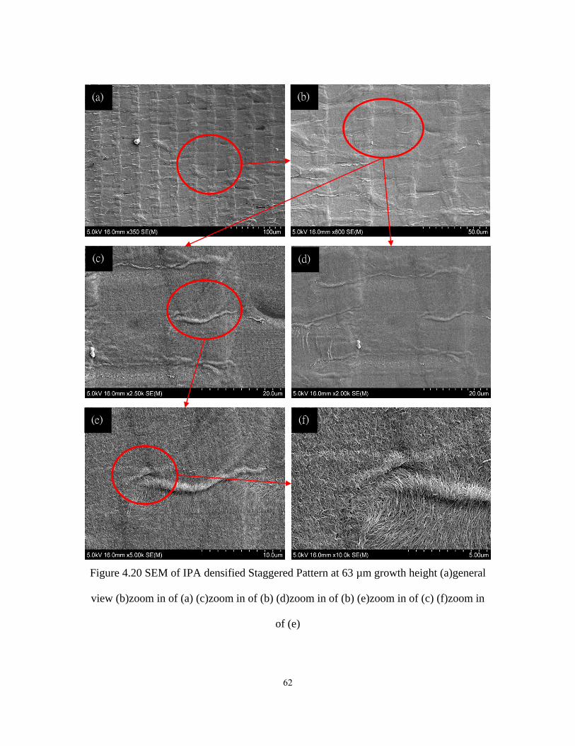
46 µm. Figure 4.20 shows the SEM of IPA densified sample at 63 µm growth height.

It is observed that, when the growth height is too long, the alignment of CNTs features

is not as perfect as shorter growth height, which also explains the decrease in Fracture

Toughness as growth height increases.

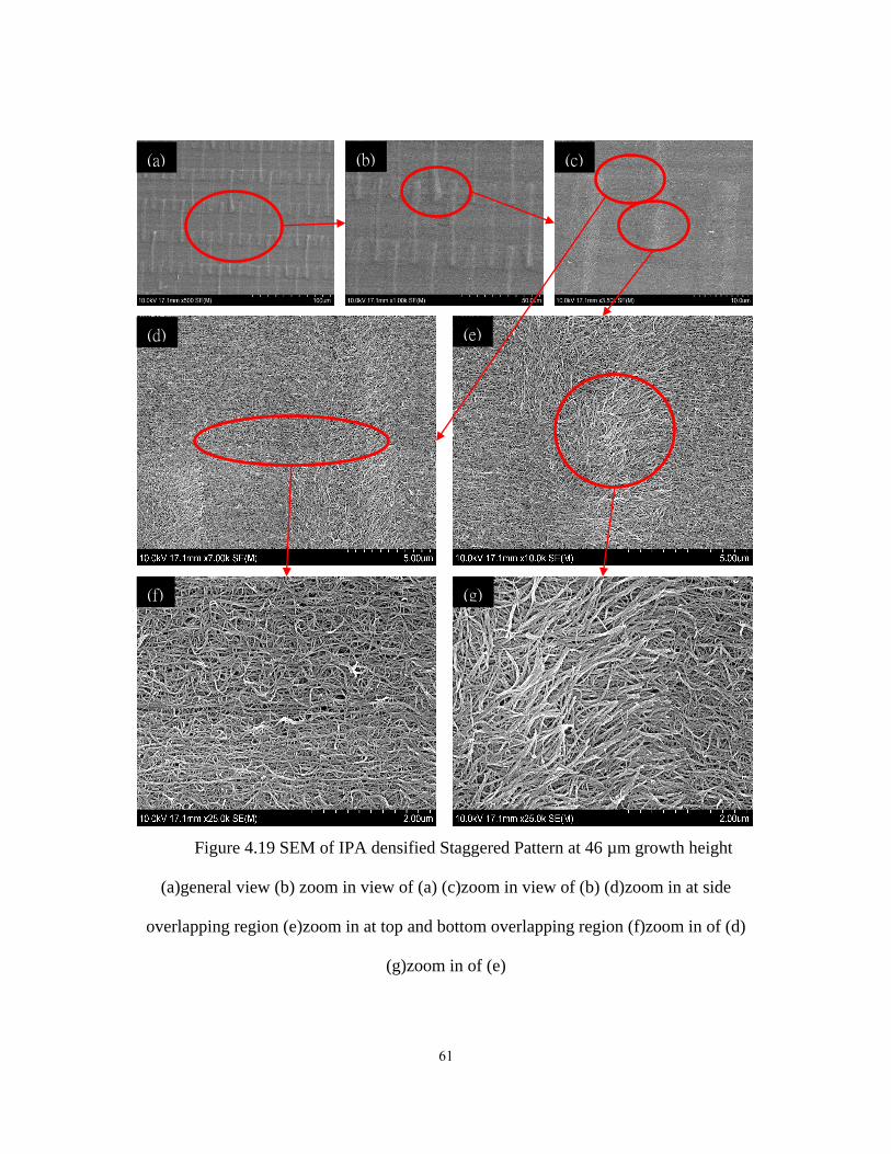
61

Figure 4.19 SEM of IPA densified Staggered Pattern at 46 µm growth height

(a)general view (b) zoom in view of (a) (c)zoom in view of (b) (d)zoom in at side

overlapping region (e)zoom in at top and bottom overlapping region (f)zoom in of (d)

(g)zoom in of (e)

(a) (b) (c)

(d) (e)

(f) (g)

62

Figure 4.20 SEM of IPA densified Staggered Pattern at 63 µm growth height (a)general

view (b)zoom in of (a) (c)zoom in of (b) (d)zoom in of (b) (e)zoom in of (c) (f)zoom in

of (e)

(a) (b)

(c) (d)

(e) (f)

63

4.8 Fractography of Broken Samples

Figure 4.21 shows SEMs of broken samples of Line Pattern. Figure 4.22 shows

SEMs of broken sample of Staggered Pattern. From both Figure 4.21 and Figure 4.22, we

can observe that the main failure mode is separation of individual feature along the

overlapping region. Along with these pulled out features are pulled out CNT fibers.

Figure 4.21 SEMs of broken sample of Line Pattern

64

Figure 4.22 SEMs of broken samples of Staggered Pattern

65

4.9 Discussion and Comparison of Different Patterns

Comparing Line Patterns, it is observed that Line (30 x 400) behaves better than Line

(50 x 400) in both electrical conductivity and mechanical strength properties. Line (30 x

400) has a thickness of 30 µm as grown, and 0.515 µm after IPA densification. Line (50 x

400) has a thickness of 50µm as grown, and 2.476 µm after IPA densification. Line (30 x

400) is densified much more than Line (50 x 400), which results in more penetration

between overlapping region. Thus, the contact between overlapping region for Line (30 x

400) is more robust than Line (50 x 400).

Comparing Line (30 x 400) and Staggered Pattern, it is observed that Staggered

Pattern behaves better in mechanical strength. While Line (30 x 400) behaves better in

electrical conductivity. The better performance in mechanical strength of Staggered Pattern

is resulted from the fact that there are more overlapping regions in Staggered Pattern, which

makes it harder to pull out individual features apart.

66

CHAPTER 5 CONCLUSIONS AND FUTURE WORK

Micro-architectured CNT sheets exhibit good mechanical and electrical properties.

For Line (30 x400) Pattern, values of tensile strength ranges from 66.8 MPa to 370.2 MPa.

Values of electrical conductivity ranges from 30.9 kS/m to 77.1 kS/m. For Line (50 x 400)

Pattern, values of tensile strength ranges from 17.4 MPa to 106.8 MPa. Values of electrical

conductivity ranges from 7.8 kS/m to 27.9 kS/m. For Staggered Pattern, values of tensile

strength ranges from 62.8 MPa to 404.1 MPa. Values of electrical conductivity ranges from

6.5 kS/m to 25.4 kS/m. Among the three patterns, Staggered Pattern behaves the best due

to its large overlapping area. This makes this pattern suitable for many potential

applications, including aerospace, smart material, actuator, and etc.

My conclusion is that thinner line thicknesses lead to better properties. Also there is a

trade-off between growing higher CNTs to get more overlap, and the effective lower of

stress due to added cross sectional area. My conclusion is that effective load transfer among

overlapping lines occur only at the contacting interface among them.

For future work, a more accurate electrical conductivity test needs to be carried out

for Staggered Pattern. This requires controlled measurement of resistance and accurate

approximation of the cross sectional area. In addition, CNT sheets of Staggered Pattern

will be utilized as composite fillers, where PMMA, PVA and other polymers will be tested

as composite matrix. Moreover, CNT-composite actuators will be developed utilizing these

composite materials.

67

APPENDIX

Both Constant Force and Pre-Stretch share the same Main Code. The only difference

is in Read Input Module and Finalized Forces Function. All modules are attached below.

Main Code

clc; clear all;

%% CNT FEA

% Variables definition

% nnode_ele, the (integer) number of nodes per element

% node_dof, the (integer) number of degrees of freedom per node

% edof, the (integer) number of degrees of freedom per element

NNODE_ELE = 2; %Number of nodes per element

DOF_NODE = 1; %Number of degrees of freedom per node

EDOF = NNODE_ELE*DOF_NODE; %number of degrees of freedom per element

%% Read Input File

[N_NODE,N_ELEM,N_LOAD,N_PRE_DISP,...

ELEM_NODE,ELEM_STIFF,COORDS,STEP_NUMBER,...

FORCE_NODE,FORCE_VAL,DISP_NODE,DISP_VAL, Force, DIS, k1, k2] =

ReadInput(NNODE_ELE);

%% Call your Initialize Equation Module

[EQ_NUM, N_DOF] = InitialEq(N_NODE,N_PRE_DISP, DISP_NODE); % Creat +(free)/-

(prescribed) values for each node for partition. EQ_NUM will be called when

stiffness/force/displacement matrix need partition

%% Call your Assemble Module

% Displacement Assemble Module

[UP] = DisplacementModule(N_PRE_DISP, DISP_NODE,DISP_VAL, EQ_NUM); % Creat

UP Matrix

for n = 1:STEP_NUMBER %Stepping starts here

% Force Assemble Module

[PF] = ForceAssembleModule(N_DOF, FORCE_NODE, FORCE_VAL, EQ_NUM, N_LOAD);

%Creat PF Matrix

68

% Global Stiffness Assemble Module

KPP = zeros(N_PRE_DISP,N_PRE_DISP); %Initialize K matrix

KPF = zeros(N_PRE_DISP,N_DOF);

KFF = zeros(N_DOF,N_DOF);

KFP = zeros(N_DOF,N_PRE_DISP);

for ELEM_NUM = 1:N_ELEM

k = ELEM_STIFF(ELEM_NUM);

node1 = ELEM_NODE(1,ELEM_NUM);

node2 = ELEM_NODE(2,ELEM_NUM);

y = COORDS(node2,2)-COORDS(node1,2);

x = COORDS(node2,1)-COORDS(node1,1);

theta = atan2(y,x);

KEL = k*[1 -1; -1 1];

c = cos(theta);

s = sin(theta);

T = [c 0; s 0; 0 c; 0 s];

KEL = T*KEL*T';

[KFF,KFP,KPF,KPP] = AssembleGlobalStiffness(KPP, KPF, KFP, KFF, EQ_NUM,

node1,node2,KEL); % Assemble stiffness value into four K matrix according to EQ_NUM

% Inclined Support

% Call Assemble Inclined Support Module

[C,q,mu] = AssembleInclinedSupport(N_DOF, KFF);

KFF = KFF + mu*C'*C;

PF = PF + mu*C'*q;

end

%% Call your Solve Module

[UUR,PUR]=SolveModule(N_NODE,KFF,KFP,KPP,KPF,UP,PF,EQ_NUM);

% Call Finalized Values Module

[URFINAL,PRFINAL,FinalPosition] = FinalizedValues(N_NODE,UUR,PUR,COORDS);

% Call Finalized Force Module

[Angle,FORCE_VAL] = FinalizedForce(N_NODE,FinalPosition,Force);

% Redefined COORDS

COORDS = FinalPosition; %Loop into another step with new force and coords

% Calculate Work

69

[WORK] = WorkLoop(N_NODE,NNODE_ELE,Force,Angle,URFINAL);

end

%% Post Processing

[SUM_WORK,SUM_PE,SUM_TOTAL_WORK,RATIO] =

PostEnergyCalculation(N_ELEM,ELEM_NODE,FinalPosition,ELEM_STIFF,DIS,k1,k2,WORK

);

% Print Output

FinalPosition

SUM_WORK

SUM_PE

SUM_TOTAL_WORK

RATIO

Read Input – Constant Force

function [N_NODE,N_ELEM,N_LOAD,N_PRE_DISP,...

ELEM_NODE,ELEM_STIFF,COORDS,STEP_NUMBER...

FORCE_NODE,FORCE_VAL,DISP_NODE,DISP_VAL, Force, DIS, k1, k2] =

ReadInput(nnode_ele)

% INPUT:

% filen: name of the file with input values

% nnode_ele: number of nodes per element

% OUTPUT:

% N_NODE, the (integer) number of nodes

% N_ELEM, the (integer) number of elements

% N_LOAD, the (integer) number of nonzero nodal forces, i.e. Pf

% N_PRE_DISP, the (integer) number of nodes with prescribed displacement, i.e. Up

% ELEM_NODE(nnode_ele, N_ELEM), matrix that contains node numbers (integers) for each

element

% ELEM_STIFF(N_ELEM), vector that contains stiffness value (real) for each element

% FORCE_NODE(N_LOAD), vector that contains the node numbers (integer) where forces are

applied

% FORCE_VAL(N_LOAD), vector that contains the value of the forces (real) corresponding to

the numbers in FORCE_NODE

% DISP_NODE(N_PRE_DISP), vector that contains the node numbers (integer) where boundary

conditions are imposed

70

% DISP_VAL(N_PRE_DISP), vector that contains the value of the forces (real) corresponding

to the numbers in DISP_NODE

% COORDS, Coordinate of each node

% STEP_NUMBER, steps you want to do per run

%% Initial Values

N_NODE = 30;

N_ELEM = 38;

N_LOAD = 15;

N_PRE_DISP = 43;

STEP_NUMBER = 150; % Change this to change #of steps

%% Stiffness Input

k1 = 10^10; %Change k1 to change stiffness of grounded node

k2 = 10^8; %Change k2 to change stiffness of each element

ELEM_STIFF =

[k1;k1;k2;k1;k1;k2;k1;k1;k2;k1;k1;k2;k1;k1;k2;k2;k1;k1;k2;k2;k1;k1;k2;k2;k2;k2;k1;k1;k2;k2;k

1;k1;k2;k2;k2;k1;k1;k2];

ELEM_NODE = [1 2 2 4 5 5 7 8 8 10 11 2 13 14 5 5 16 17 8 8 19 20 11 14 17 14 22

23 17 17 25 26 20 23 23 28 29 26 ;...% Connection between node to node;

2 3 5 5 6 8 8 9 11 11 12 14 14 15 14 17 17 18 17 20 20 21 20 17 20 23 23 24 23

26 26 27 26 26 29 29 30 29]; % Corresponding to the stiffness of each element;

%% Force Input and loops

Angle = [30 30 30 60 60 60 -60 -60 -60 -30 -30 -30 0 0 0 0 0 0 0 0 0 -60 -60 -60 60 60 60 -90 -90

-90]; % Angle between each node to the fixed node(node 17)

Force = 1; %Change applied force

FORCE_NODE = [2 1; 2 2; 5 1; 5 2; 8 1; 8 2; 11 1; 11 2; 14 1; 20 1; 23 1; 23 2; 26 1; 26 2; 29 2];

FORCE_VAL = Force*[cosd(Angle(2)), sind(Angle(2)),...

cosd(Angle(5)), sind(Angle(5)),...

-cosd(Angle(8)), -sind(Angle(8)),...

-cosd(Angle(11)), -sind(Angle(11)), ...

cosd(Angle(14)),...

-cosd(Angle(20)),...



sind(Angle(29))]';

71

%% Displacement Input

DISP_NODE = [1 1; 1 2; 3 1; 3 2; 4 1; 4 2; 6 1; 6 2; 7 1; 7 2; 9 1; 9 2; 10 1; 10 2; 12 1; 12 2; 13

1; 13 2;...

15 1; 15 2; 16 1; 16 2; 17 1; 17 2; 18 1; 18 2; 19 1; 19 2; 21 1; 21 2; 22 1; 22 2; 24 1; 24 2;

25 1; 25 2;...

27 1; 27 2; 28 1; 28 2; 29 1; 30 1; 30 2]; % Prescribed displacement nodes; mainly the

grounded node; Plus the fixed node;

DISP_VAL = zeros(N_PRE_DISP,1);

%% COORDS Input

r = 20*10^-9; %Ideally this part is always fixed

DIS = r*2;

COORDS = [0 0; 0 0; 0 0;...

2*r 0; 2*r 0; 2*r 0;...

4*r 0; 4*r 0; 4*r 0;...

6*r 0; 6*r 0; 6*r 0;...

r sqrt(3)*r; r sqrt(3)*r; r sqrt(3)*r;...

3*r sqrt(3)*r; 3*r sqrt(3)*r; 3*r sqrt(3)*r;...


2*r 2*sqrt(3)*r; 2*r 2*sqrt(3)*r; 2*r 2*sqrt(3)*r;...


3*r 3*sqrt(3)*r; 3*r 3*sqrt(3)*r; 3*r 3*sqrt(3)*r];

Read Input – Pre-stretch

function [N_NODE,N_ELEM,N_LOAD,N_PRE_DISP,...

ELEM_NODE,ELEM_STIFF,COORDS,STEP_NUMBER,...

FORCE_NODE,FORCE_VAL,DISP_NODE,DISP_VAL,Force, DIS, k1, k2] =

ReadInput(nnode_ele)

% INPUT:

% filen: name of the file with input values

% nnode_ele: number of nodes per element

% OUTPUT:

% N_NODE, the (integer) number of nodes

% N_ELEM, the (integer) number of elements

% N_LOAD, the (integer) number of nonzero nodal forces, i.e. Pf

% N_PRE_DISP, the (integer) number of nodes with prescribed displacement, i.e. Up

72

% ELEM_NODE(nnode_ele, N_ELEM), matrix that contains node numbers (integers) for each

element

% ELEM_STIFF(N_ELEM), vector that contains stiffness value (real) for each element

% FORCE_NODE(N_LOAD), vector that contains the node numbers (integer) where forces are

applied

% FORCE_VAL(N_LOAD), vector that contains the value of the forces (real) corresponding to

the numbers in FORCE_NODE

% DISP_NODE(N_PRE_DISP), vector that contains the node numbers (integer) where boundary

conditions are imposed

% DISP_VAL(N_PRE_DISP), vector that contains the value of the forces (real) corresponding

to the numbers in DISP_NODE

%% Initial Values

N_NODE = 30;

N_ELEM = 38;

N_LOAD = 18;

N_PRE_DISP = 43;

STEP_NUMBER = 1;

%% Stiffness Input

k1 = 10^6;

k2 = 10^9;

ELEM_STIFF =

[k1;k1;k2;k1;k1;k2;k1;k1;k2;k1;k1;k2;k1;k1;k2;k2;k1;k1;k2;k2;k1;k1;k2;k2;k2;k2;k1;k1;k2;k2;k

1;k1;k2;k2;k2;k1;k1;k2];

ELEM_NODE = [1 2 2 4 5 5 8 9 8 10 11 2 13 14 5 5 16 17 8 8 20 21 11 14 17 14 22

23 17 17 26 27 20 23 23 28 29 26;...

2 3 5 5 6 8 7 8 11 11 12 14 14 15 14 17 17 18 17 20 19 20 20 17 20 23 23 24 23

26 25 26 26 26 29 29 30 29];

%% Force Input and Loops

Angle = [0 0 0 60 -60 60 -60 60 -60];

Force = 30;

FORCE_NODE = [2 1; 2 2; 5 1; 5 2; 8 1; 8 2; 11 1; 11 2; 14 1; 14 2; 20 1; 20 2; 23 1; 23 2; 26 1;

26 2; 29 1; 29 2];

FORCE_VAL = Force*[cosd(Angle(4))+cosd(Angle(1)), sind(Angle(4))+sind(Angle(1)), ...

cosd(Angle(2))-cosd(Angle(1)), sind(Angle(2))-sind(Angle(1)),...

73


-cosd(Angle(5))-cosd(Angle(3)), -sind(Angle(5))+sind(Angle(3)),...





cosd(Angle(9))-cosd(Angle(8)), sind(Angle(9))-sind(Angle(8))];

%% Displacement Input

r = 20*10^-9;

DIS = 2*r;

DISP_NODE = [1 1; 1 2; 3 1; 3 2; 4 1; 4 2; 6 1; 6 2; 7 1; 7 2; 9 1; 9 2; 10 1; 10 2; 12 1; 12 2; 13

1; 13 2;...

15 1; 15 2; 16 1; 16 2;17 1; 17 2;

18 1; 18 2; 19 1; 19 2; 21 1; 21 2; 22 1; 22 2; 24 1; 24 2; 25 1; 25 2;...

27 1; 27 2; 28 1; 28 2;29 1;

30 1; 30 2;];

DISP_VAL = zeros(N_PRE_DISP,1);

%% COORDS Input

COORDS = [0 0; 0 0; 0 0;...

2*r 0; 2*r 0; 2*r 0;...

4*r 0; 4*r 0; 4*r 0;...

6*r 0; 6*r 0; 6*r 0;...

r sqrt(3)*r; r sqrt(3)*r; r sqrt(3)*r;...





3*r 3*sqrt(3)*r; 3*r 3*sqrt(3)*r; 3*r 3*sqrt(3)*r];

Initialize Equation Module

function [EQ_NUM, N_DOF] = InitialEq(N_NODE,N_PRE_DISP, DISP_NODE)

EQ_NUM = zeros(N_NODE*2,1);

for i= 1:N_PRE_DISP

if DISP_NODE(i,2) == 1

NODE = 2*DISP_NODE(i,1)-DISP_NODE(i,2);

74

else if DISP_NODE(i,2) ==2

NODE = 2*DISP_NODE(i,1);

end

end

EQ_NUM(NODE) = -i;

end

ROW = 0;

for i = 1:N_NODE*2

if (EQ_NUM(i) == 0)

ROW = ROW + 1;

EQ_NUM(i) = ROW;

end

end

N_DOF = N_NODE*2 - N_PRE_DISP;

Displacement Assemble Module

function [UP] = DisplacementModule(N_PRE_DISP, DISP_NODE, DISP_VAL, EQ_NUM)

UP = zeros(N_PRE_DISP,1);

for i = 1:N_PRE_DISP

if DISP_NODE(i,2) == 1

NODE = 2*DISP_NODE(i,1)-DISP_NODE(i,2);

else if DISP_NODE(i,2) ==2

NODE = 2*DISP_NODE(i,1);

end

end

ROW = -EQ_NUM(NODE);

UP(ROW) = UP(ROW)+ DISP_VAL(i);

End

Force Assemble Module

function [PF] = ForceAssembleModule(N_DOF, FORCE_NODE, FORCE_VAL, EQ_NUM,

N_LOAD)

PF = zeros(N_DOF,1);

for i = 1:N_LOAD

if FORCE_NODE(i,2) == 1

NODE = 2*FORCE_NODE(i,1)-FORCE_NODE(i,2);

75

else if FORCE_NODE(i,2) ==2

NODE = 2*FORCE_NODE(i,1);

end

end

ROW = EQ_NUM(NODE);

if (ROW > 0)

PF(ROW) = PF(ROW)+FORCE_VAL(i);

end

end

Stiffness Assemble Module

function [KFF,KFP,KPF,KPP] = AssembleGlobalStiffness(KPP, KPF, KFP, KFF, EQ_NUM,

node1,node2,KEL)

for i = 1:4

ROW1 = EQ_NUM(2*node1-1);

ROW2 = EQ_NUM(2*node1);

ROW3 = EQ_NUM(2*node2-1);

ROW4 = EQ_NUM(2*node2);

ROW = [ROW1,ROW2,ROW3,ROW4];

for j = 1:4

COL1 = EQ_NUM(2*node1-1);

COL2 = EQ_NUM(2*node1);

COL3 = EQ_NUM(2*node2-1);

COL4 = EQ_NUM(2*node2);

COL = [COL1,COL2,COL3,COL4];

if (ROW(i) > 0)

if (COL(j) > 0)

KFF(ROW(i),COL(j)) = KFF(ROW(i),COL(j)) + KEL(i,j);

else

KFP(ROW(i),-COL(j)) = KFP(ROW(i),-COL(j)) + KEL(i,j);

end

else

if (COL(j) > 0)

KPF(-ROW(i),COL(j)) = KPF(-ROW(i),COL(j)) + KEL(i,j);

else

76

KPP(-ROW(i),-COL(j)) = KPP(-ROW(i),-COL(j)) + KEL(i,j);

end

end

end

end

Inclined Support Assemble Module

function[C,q,mu] = AssembleInclinedSupport(N_DOF, KFF)

C = zeros(1,N_DOF);

C(1) = sind(30);

C(2) = -cosd(30);

C(7) = sind(30);

C(8) = cosd(30);

q = 0;

mu = 10^15;

% mu = 10^5*max(max(abs(KFF)));

Solve Module

function[UUR,PUR]=SolveModule(N_NODE,KFF,KFP,KPP,KPF,UP,PF,EQ_NUM)

UUR = zeros(N_NODE*2,1);

PUR = zeros(N_NODE*2,1);

UF = KFF\(PF - KFP*UP);

PP = KPP*UP + KPF*UF;

for i = 1:N_NODE*2

ROW = EQ_NUM(i);

if (ROW > 0)

UUR(i) = UF(ROW);

PUR(i) = PF(ROW);

else

UUR(i) = UP(-ROW);

PUR(i) = PP(-ROW);

end

end

Finalized Values

function[URFINAL,PRFINAL,FinalPosition] =

77

FinalizedValues(N_NODE,UUR,PUR,COORDS)

%Final Position

URFINAL = zeros(N_NODE,2);

countj = 1;

for j = 1: N_NODE

URFINAL(j,1) = UUR(countj,1);

URFINAL(j,2) = UUR(countj+1,1);

countj = countj + 2;

end

%Final Reaction Force

PRFINAL = zeros(N_NODE,2);

countl = 1;

for l = 1: N_NODE

PRFINAL(l,1) = PUR(countl,1);

PRFINAL(l,2) = PUR(countl+1,1);

countl = countl + 2;

end

FinalPosition = URFINAL+COORDS;

Finalized Force – Constant Force

function[Angle,FORCE_VAL] = FinalizedForce(N_NODE,FinalPosition,Force)

Angle = zeros(N_NODE,1);

for m = 1:N_NODE

Angle(m) = atand((FinalPosition(18,2)-FinalPosition(m,2))/(FinalPosition(18,1)-

FinalPosition(m,1)));

end

% Redirected Force based on final angle

FORCE_VAL = Force*[cosd(Angle(2)), sind(Angle(2)),...



-cosd(Angle(11)), -sind(Angle(11)), ...

cosd(Angle(14)),...

-cosd(Angle(20)),...



78

sind(Angle(29))]';

Finalized Force – Pre-Stretch

function[Angle,FORCE_VAL] = FinalizedForce(FinalPosition,Force)

Angle = zeros(9,1);

% Angle = [atand((FinalPosition(5,2)-FinalPosition(2,2))/(FinalPosition(5,1)-

FinalPosition(2,1))),...

% 0,...

% -atand((FinalPosition(5,2)-FinalPosition(2,2))/(FinalPosition(5,1)-FinalPosition(2,1))),...

% atand((FinalPosition(5,2)-FinalPosition(2,2))/(FinalPosition(5,1)-FinalPosition(2,1))),...



% atand((FinalPosition(5,2)-FinalPosition(2,2))/(FinalPosition(5,1)-FinalPosition(2,1))),...


% atand((FinalPosition(5,2)-FinalPosition(2,2))/(FinalPosition(5,1)-FinalPosition(2,1)))];

Angle = [atand((FinalPosition(5,2)-FinalPosition(2,2))/(FinalPosition(5,1)-FinalPosition(2,1))),...

atand((FinalPosition(8,2)-FinalPosition(5,2))/(FinalPosition(8,1)-FinalPosition(5,1))),...







atand((FinalPosition(29,2)-FinalPosition(26,2))/(FinalPosition(29,1)-FinalPosition(26,1)))];

FORCE_VAL = Force*[cosd(Angle(4))+cosd(Angle(1)), sind(Angle(4))-sind(Angle(1)), ...



-cosd(Angle(5))-cosd(Angle(3)), -sind(Angle(5))+sind(Angle(3)),...





cosd(Angle(9))-cosd(Angle(8)), sind(Angle(9))-sind(Angle(8))];

Work Loop

function[WORK] = WorkLoop(N_NODE,NNODE_ELE,Force,Angle,URFINAL)

79

WORK = zeros(N_NODE,NNODE_ELE);

WORK = WORK + Force.*[0 0; cosd(Angle(2)), sind(Angle(2)); 0 0;...

0 0; cosd(Angle(5)), sind(Angle(5)); 0 0;...

0 0; -cosd(Angle(8)), -sind(Angle(8));0 0;...

0 0; -cosd(Angle(11)), -sind(Angle(11));0 0; ...

0 0; cosd(Angle(14)), 0; 0 0; 0 0; 0 0; 0 0;...

0 0; -cosd(Angle(20)), 0; 0 0;...

0 0; cosd(Angle(23)), sind(Angle(23)); 0 0;...

0 0; -cosd(Angle(26)), -sind(Angle(26)); 0 0;...

0 0; 0 sind(Angle(29)); 0 0].*URFINAL;

Post Processing

function[SUM_WORK,SUM_PE,SUM_TOTAL_WORK,RATIO] =

PostEnergyCalculation(N_ELEM,ELEM_NODE,FinalPosition,ELEM_STIFF,DIS,k1,k2,WORK

)

% New Element Length

LengthX = zeros(N_ELEM,1);

LengthY = zeros(N_ELEM,1);

Length = zeros(N_ELEM,1);

for i = 1:N_ELEM

ELE_NODE = ELEM_NODE';

LengthX(i) = FinalPosition(ELE_NODE(i,2),1)-FinalPosition(ELE_NODE(i,1),1);

LengthY(i) = FinalPosition(ELE_NODE(i,2),2)-FinalPosition(ELE_NODE(i,1),2);

Length(i) = sqrt(LengthX(i).^2+LengthY(i).^2);

end

% Change in Length

Dlength = zeros(N_ELEM,1);

for i = 1:N_ELEM

if ELEM_STIFF(i) == k1

Dlength(i) = Length(i);

else if ELEM_STIFF(i) == k2

Dlength(i) = Length(i)-DIS;

end

end

end

80

% Potential Energy

PE = zeros(N_ELEM,1);

PE = 0.5.*ELEM_STIFF.*(Dlength.^2);

% Energy Calculation

SUM_WORK = sum(WORK);

SUM_PE = sum(PE);

SUM_TOTAL_WORK = sum(SUM_WORK);

RATIO = SUM_TOTAL_WORK/SUM_PE;

81

REFERENCES

[1] R.S. Ruoff et al., C. R. Physique 4 (2003).

[2] Zhang et al., ACS Nano, (2013), 7 (7), pp 6156–6161.

[3] S. Iijima, Nature 354 (6348) (1991) 56–58.

[4] T.W. Ebbesen, P.M. Ajayan, Nature 358 (6383) (1992) 220–222.

[5] S. Iijima, P.M. Ajayan, T. Ichihashi, Phys. Rev. Lett. 69 (21) (1992) 3100–3103

[6] A. Thess, R. Lee, P. Nikolaev, H.J. Dai, P. Petit, J. Robert, C.H. Xu, Y.H. Lee, S.G.

Kim, A.G. Rinzler, D.T. Colbert, G.E. Scuseria, D. Tomanek, J.E. Fischer, R.E.

Smalley, Science 273 (5274) (1996) 483–487.

[7] T. Guo, P. Nikolaev, A. Thess, D.T. Colbert, R.E. Smalley, Chem.Phys. Lett. 243

(1–2) (1995) 49–54.

[8] J. Kong, H.T. Soh, A.M. Cassell, C.F. Quate, H.J. Dai, Nature 395 (6705) (1998)

878–881.

[9] A.M. Cassell, J.A. Raymakers, J. Kong, H.J. Dai, J. Phys.Chem. B 103 (31) (1999)

6484–6492.

[10] W.Z. Li, S.S. Xie, L.X. Qian, B.H. Chang, B.S. Zou, W.Y. Zhou, R.A. Zhao, G.

Wang, Science 274 (5293) (1996) 1701–1703

[11] M.F. Yu, O. Lourie, M.J. Dyer, K. Moloni, T.F. Kelly, R.S. Ruoff, Science 287

(5453) (2000) 637–640.

[12] Z.W. Pan, S.S. Xie, L. Lu, B.H. Chang, L.F. Sun, W.Y. Zhou, G. Wang, D.L. Zhang,

Appl. Phys. Lett. 74 (21) (1999) 3152–3154

82

[13] J.J Vilatela, J.A. Elliott, A.H. Windle, ACS Nano. 5 (3) (2011) 1921-1927.

[14] M. Miao, CARBON 49 (2011), 3755 – 3761

[15] Zhong XY, Li YL, Liu YK, Qiao XH, Feng Y, Liang J, et al, Adv Mater, (2010)

;22:692–6.

[16] S. Tawfick, K. O’Brien, A. J. Hart , Small (2009), 5, No. 21, 2467–2473

[17] M. D. Volder , S. H. Tawfick , S. J. Park , D. Copic , Z. Zhao , W. Lu , and A. J. Hart

Adv. Mater, (2010), 22, 4384-4389

[18] D. N. Futaba1, K. Hata*, T. Yamada, T. Hiraoka, Y. Hayamizu, Y. Kakudate, O.

Tanaike, H. Hatori, M. Yumura, And S. Iijima, Nature Materials. (2016), Vol 5, 987-

994

[19] S. Tawfick, Z. Zhao, M. Maschmann, A. Brieland-Shoultz, M. D. Volder, J. W. Baur,

W.Lu, and A. J. Hart*, Langmuir, (2013), 29, 5190-5198

mechanical and electrical properties of micro

Documents