mechanically versatile soft machines through laminar jamming
TRANSCRIPT

Mechanically Versatile Soft MachinesThrough Laminar Jamming
Yashraj S. Narang1, Joost J. Vlassak1, and Robert D. Howe1*
1Paulson School of Engineering and Applied Sciences, Harvard University, Cambridge, MA02138
*Corresponding author: Email [email protected]
Abstract
There are two major structural paradigms in robotics: soft machines, which are conformable,durable, and safe for human interaction; and traditional rigid robots, which are fast, precise,and capable of applying high forces. Here, we bridge the paradigms by enabling soft machinesto behave like traditional rigid robots on command. To do so, we exploit laminar jamming, astructural phenomenon in which a laminate of compliant strips becomes strongly coupled throughfriction when a pressure gradient is applied, causing dramatic changes in mechanical properties. Wedevelop rigorous analytical and finite element models of laminar jamming, and we experimentallycharacterize jamming structures to show that the models are highly accurate. We then integratejamming structures into soft machines to enable them to selectively exhibit the stiffness, damping,and kinematics of traditional rigid robots. The models allow jamming structures to be rapidlydesigned to meet arbitrary performance specifications, and the physical demonstrations illustratehow to construct systems that can behave like either soft machines or traditional rigid robots atwill, such as continuum manipulators that can have joints appear and disappear. Our study aimsto foster a new generation of mechanically versatile machines and structures that cannot simplybe classified as “soft” or “rigid.”
Soft machines and traditional rigid robotshave distinct forms and functions. Soft ma-
chines (e.g., elastomeric bending actuators[1, 2]and dielectric elastomer grippers[3, 4]) are madeof compliant materials and bend or twist contin-uously along their length. Their actuation mech-anism is typically distributed throughout theirvolume. Traditional rigid robots (e.g., roboticarms and humanoids) are made of stiff materials
and bend or translate discretely at joints. Theiractuation mechanism is usually confined to thesejoints. The structure of soft machines allowsthem to conform to complex shapes[5, 6], with-stand crushing loads[7], dampen impacts, and in-teract safely with the body[8, 9]. In contrast, thestructure of traditional rigid robots enables themto perform tasks quickly, precisely, and with highresolution, as well as resist deformation, apply
Submission to Advanced Functional Materials Page 1
“Mechanically Versatile Soft Machines Through Laminar Jamming” Narang, Vlassak, and Howe
high forces, and oscillate with minimal decay.To make more versatile robots, researchers
have aimed to enable soft machines to selec-tively behave like traditional rigid robots. Inparticular, soft machines have been constructedwith materials and structures that can ex-hibit tunable stiffness and damping in orderto attain the mechanical properties of tradi-tional robots. These components include low-melting-point materials[10, 11], shape-memorymaterials[12, 13], magnetorheological fluids[14],and granular structures[15, 9]. Nevertheless,most of these technologies cannot achieve awide range of stiffness and damping values perunit weight, have low resolution of stiffness anddamping values, transition between these val-ues slowly, and/or have poor resistance to bend-ing moments[9, 16]. Furthermore, none of thesetechnologies have yet enabled continuously de-forming soft machines to selectively exhibit thediscrete, jointed kinematics of traditional robots.
The laminar jamming (a.k.a.,“layer jam-ming”) phenomenon is a promising alternativeto these technologies (Figure 1A-B). Laminarjamming structures are lightweight and can berapidly actuated; moreover, they can achieveexcellent range and resolution of stiffness anddamping values with high resistance to bendingmoments. A laminar jamming structure consistsof a laminate of flexible strips or sheets. In itsdefault state, the laminate is highly compliant.However, when a pressure gradient is applied (inthis study, by enclosing the laminate in an air-tight envelope and applying a vacuum to theenvelope), increased frictional interactions dra-matically augment the bending stiffness of thestructure; in addition, at high loads, the struc-ture dissipates energy. Researchers have appliedlaminar jamming to haptics[17, 18, 19], medicaldevices[20, 21], and soft actuators[22, 23]. Nev-
ertheless, these studies have not yet providedanalytical or computational models for laminarjamming beyond an initial deformation phase,making design of practical jamming structuresan arduous process. Furthermore, they have notyet explored how laminar jamming can be usedto transform bending kinematics.
In this paper, we model laminar jamming indetail and demonstrate how the technology canbridge the gap between soft machines and tra-ditional rigid robots. Specifically, we develop ananalytical model that mathematically captureshow two-layer jamming structures behave overall major phases of deformation. We then de-velop finite element models that extend thesepredictions to many-layer jamming structures,as well as describe how their stiffness and damp-ing depend on critical design inputs (e.g., thevacuum pressure). These models are validatedthrough rigorous experimental characterization.Together, the analytical and finite element mod-els present researchers with the first means torapidly and accurately design jamming struc-tures to meet arbitrary design requirements.
We then demonstrate the capabilities of lami-nar jamming structures by integrating them intoreal-world pneumatic and cable-driven soft ma-chines. In the process, we achieve two novelfunctions that illustrate how these machines canreversibly emulate traditional rigid robots: 1)shape-locking, in which a compliant system canselectively manifest a stiff version of a desiredshape and preserve it, even after powering off theactuators, and 2) variable kinematics, in whicha compliant system can transition between con-tinuous bending and discrete, jointed bending oncommand. The variable kinematics function isthen used to build a two-fingered grasper thatcan perform pinch grasps on small objects, aswell as wrap grasps on objects of eight times the
Initial Submission to Advanced Functional Materials Page 2

“Mechanically Versatile Soft Machines Through Laminar Jamming” Narang, Vlassak, and Howe
A
Airtight envelopeVacuum
line
Layers ofcompliantmaterial
C
DAp
plie
d fo
rce
Firstcritical load
Secondcritical loadTransition
regime
Full-slipregime
Vacuum off
Vacuum on
Deflection
Low sti�ness,plastic
High sti�ness,elastic
Low sti�ness,elastic
Pre-slipregime
B
Vacuum on
Vacuum on
Low/moderate force
High force
No slip
Slip
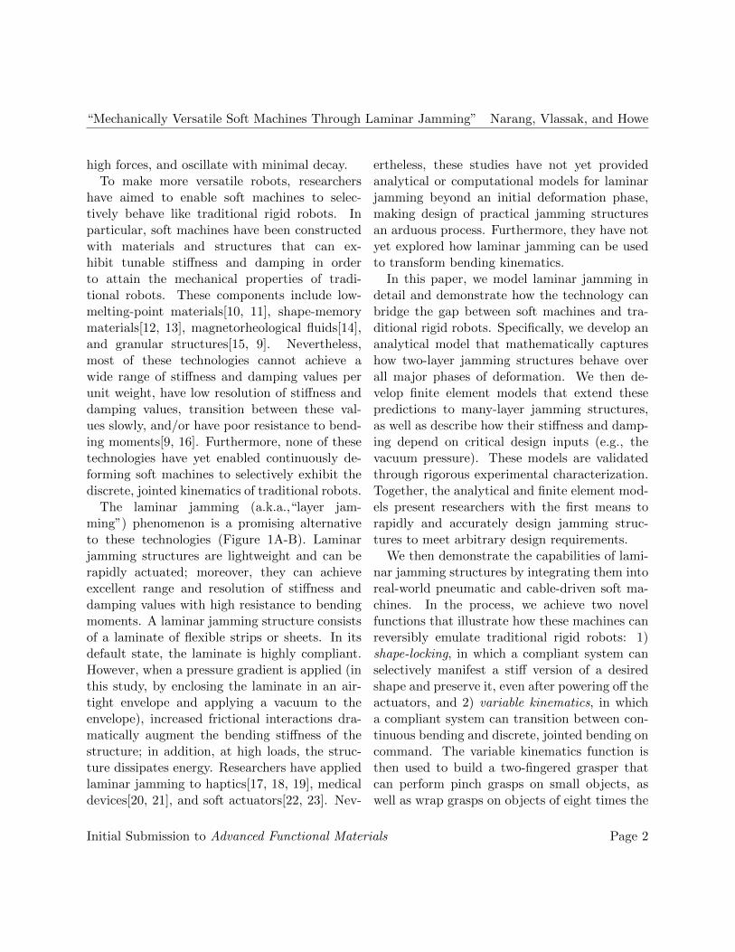
Figure 1: Fundamental behavior of laminar jamming structures. A) Schematic of a jamming structure.B) When vacuum is off, the layers bend independently, and the structure has low bending stiffness. Whenvacuum is on, the layers bend as a cohesive unit, and the structure has high bending stiffness. C) However,when vacuum is on, the layers are cohesive only until a critical force. For higher forces, longitudinal shearstress is large enough to cause the layers to slip at certain points along their interfaces. D) Summary ofmechanical behavior. When vacuum is off, the structure has low bending stiffness, which is proportional tothe slope of the curves. When vacuum is on, the structure has three deformation regimes. In pre-slip, thebending stiffness is maximal and constant. After the first critical load, the structure enters the transitionregime, in which the layers begin to slip. The bending stiffness decreases. After the second critical load, thestructure enters full-slip, in which the layers have slipped at all possible points along their interfaces. Thebending stiffness is minimal and constant. When slip occurs, energy is dissipated to friction between thelayers, and the structure behaves plastically.
Initial Submission to Advanced Functional Materials Page 3

“Mechanically Versatile Soft Machines Through Laminar Jamming” Narang, Vlassak, and Howe
diameter. These demonstrations prove the fea-sibility of using laminar jamming to build me-chanically versatile machines and structures thatexhibit both soft and traditional behavior.
Results
Analytical Modeling
As described earlier, when a vacuum is appliedto a laminar jamming structure, the bendingstiffness increases dramatically. Previous stud-ies have shown that the stiffness increases by afactor of n2, where n is the number of layersin the structure; however, the vacuumed jam-ming structure sustains this increased stiffnessonly for small loads, beyond which the stiffnessdeclines[17, 20].
In our investigation, physical reasoning sug-gested that this behavior reflected three phasesof deformation in a vacuumed jamming structure(Figure 1C-D): 1) In pre-slip, the layers are cohe-sive, and the stiffness of the structure is a factorof n2 greater than the stiffness without vacuum.No energy is dissipated, and the damping (i.e.,dissipated energy per unit deflection) is zero. Asthe structure is loaded, the longitudinal shearstress along the interfaces between layers beginsto rise. 2) In the transition regime, the longitudi-nal shear stress along certain regions of the inter-faces equals the maximum possible shear stress,which is determined by the coefficient of frictionand the pressure gradient. Layers begin to slipalong those regions, and the stiffness of the struc-ture decreases. Energy is dissipated to friction,and the damping increases. 3) In full-slip, alllayers have slipped along the full length of theirinterfaces. The stiffness of the structure is min-imal, and the damping is maximal.
To mathematically capture this behavior, we
derived an analytical model that rigorously de-scribed the deformation and mechanical proper-ties of jamming structures during these phases.Our model was based on Euler-Bernoulli beamtheory; however, we extended the theory to de-scribe how mechanical behavior was affected byvacuum pressure, friction at the interfaces be-tween layers, and slip along the interfaces. Gov-erning equations were derived using equilibriumand moment-stress relations, and general bound-ary conditions were formulated (SI: Analyt-ical Modeling: Governing Equations andBoundary Conditions). The boundary-valueproblem was then solved for a two-layer can-tilevered jamming structure under a uniform dis-tributed load (SI: Analytical Modeling: Ex-plicit Solution); this case was chosen to illus-trate slip propagation (i.e., growth of the regionsalong which layers slip), which is exhibited bymost jamming structures.
The model predicted the elastica (i.e., theshape), stiffness, dissipated energy, and damp-ing of the jamming structure. The model alsopredicted the transition loads (i.e., the loadsat which the jamming structure shifts fromone deformation phase to the next), as well asthe length of the region along which the lay-ers slipped. Furthermore, it provided the func-tional dependence of all the preceding quantitieson dimensions, material properties, the vacuumpressure, and the applied load (SI: AnalyticalModeling: Summary of Formulae). For ex-ample, the model showed that the full-slip damp-ing force was given succinctly by µPbh, whereµ is the coefficient of friction, P is the vacuumpressure, b is the width of a layer, and h is theheight. Dimensionless forms of the equations inthe model were derived as well (SI: Analyti-cal Modeling: Dimensionless Forms). Themodel was evaluated for an example structure
Initial Submission to Advanced Functional Materials Page 4

“Mechanically Versatile Soft Machines Through Laminar Jamming” Narang, Vlassak, and Howe
A
C
B
0 10 20 30 40Tip deflection [mm]
0
1
2
3
4
5
6
7
Dis
tribu
ted
load
[N/m
] Pre-slip
Transitionregime
Full-slip
AnalyticalFinite element
0
2
4
6
8
Dis
sipa
ted
ener
gy [m
J]
R2=0.9977
R2=0.9639
y
x
Vacuum pressure
Distributed load
0 50 100 150 200 250X-coordinate [mm]
-35
-30
-25
-20
-15
-10
-5
0
Y-co
ordi
nate
[mm
]
CohesiveSlipped
Increasingload
Pre-slip
Transitionregime
Full-slip
1a
1b
2
Analytical
Figure 2: Analytical model of two-layer jamming structures. A) Schematic of example jamming structure.B) Elastica of jamming structure for increasing loads. The slipped region is highlighted at each load;because shear stress decreases along the x-direction, the slipped region initiates at the clamped end andgrows toward the free end. Two-layer finite element models corroborated that slip occurred in analytically-predicted regions. C) Bending stiffness is proportional to the slope of the load-versus-deflection curve; asexpected, the stiffness transitions from a minimal to a maximal value. Damping is proportional to the slopeof the dissipated-energy-versus-deflection curve; damping transitions from zero to a maximal value. Finiteelement models closely corroborated analytically-predicted stiffness and damping values. (SI: AnalyticalModeling: Case Study)
Initial Submission to Advanced Functional Materials Page 5

“Mechanically Versatile Soft Machines Through Laminar Jamming” Narang, Vlassak, and Howe
(Figure 2), and the results were corroboratedby two-layer finite element models (SI: FiniteElement Modeling: Two-Layer JammingStructures).
Finite Element Modeling and Experi-mental Characterization
Although the analytical model rigorously pre-dicted the mechanical behavior of two-layer jam-ming structures, designers may desire to buildreal-world jamming structures with additionallayers to further adjust their properties. Ouranalytical model can be directly extended to de-scribe many-layer jamming structures (SI: An-alytical Modeling: Extending the Model).However, the process is algebraically taxing, andnumerical methods may be preferred.
To predict the mechanical behavior of many-layer jamming structures, we conducted finiteelement simulations. The jamming structureswere modeled as 2D plane-strain structures withdimensions, material properties, boundary con-ditions, and loads equal to those of real-worldjamming structures used later in experimen-tal validation (SI: Finite Element Model-ing: Stiffness and Damping of Many-LayerJamming Structures). Furthermore, simulta-neous frictional contact was allowed to occur atall interfaces, and large-deformation analysis wasenabled. No fitting parameters were used.
The results of the finite element simulationswere used to quantify how critical design inputsaffected major performance metrics of many-layer jamming structures. Specifically, the num-ber of layers, vacuum pressure, and coefficient offriction of the layers were varied, and the stiffnessand damping values of the jamming structuresduring pre-slip and full-slip were extracted. Thepolynomial relationship between each input and
output was determined, and the resulting scalingrelations were tabulated (SI: Finite ElementModeling: Functional Dependencies). Forexample, full-slip damping was found to scale lin-early with number of layers, vacuum pressure,and coefficient of friction.
To evaluate the accuracy of the finite elementmodels, experimental characterization of many-layer jamming structures was conducted. Jam-ming structures were fabricated according to amulti-step process (SI: Experimental Char-acterization: Fabrication Process), and therepeatability of the structures was assessed (SI:Experimental Characterization: Repeata-bility Analysis). The jamming structures werehighly repeatable from loading cycle to loadingcycle and sample to sample. The many-layerjamming structures were then tested in three-point bending for various numbers of layers andvacuum pressures (SI: Experimental Char-acterization: Stiffness and Damping Char-acterization Process). Transverse force andmaximum deflection was recorded, and finite el-ement predictions were compared to experimen-tal data (Figure 3). The finite element modelspredicted experimental results with exceptionalaccuracy.
Useful Functions
Shape-Locking
Two real-world capabilities of laminar jammingstructures were demonstrated by integratingthem into soft machines. First, the shape-locking function was demonstrated. A pneu-matically powered soft bending actuator wasfabricated (SI: Functions and Applications:Shape-Locking), and a twenty-layer jammingstructure was adhered to the ventral surface (i.e.,
Initial Submission to Advanced Functional Materials Page 6

“Mechanically Versatile Soft Machines Through Laminar Jamming” Narang, Vlassak, and Howe
μ=0.75
μ=0.50
μ=0.25
0 2 4 6 8Deflection [mm]
0
2
4
6
8
10
Appl
ied
forc
e [N
]
Experimental Finite element
Effect of Number of Layers(Vacuum Pressure = 71 kPa,Coefficient of Friction = 0.65)
0 2 4 6 8Deflection [mm]
Experimental Finite element
Effect of Vacuum Pressure(Number of Layers = 20,
Coefficient of Friction = 0.65)
0 2 4 6 8Deflection (mm)
Finite element
Effect of Coefficient of Friction(Number of Layers = 20,
Vacuum Pressure = 71 kPa)
5 layers
10 layers
15 layers
20 layers
0 kPa
24 kPa
47 kPa
71 kPa
Figure 3: Finite element predictions and experimental validation for many-layer jamming structures. Jam-ming structures were loaded in three-point bending. Each experimental curve in fact consists of a meancurve and shaded error bar that spans ±1 standard deviation; the maximum deviation on any curve is0.24N , indicating high repeatability. The minimum coefficient of determination (R2) between finite elementand experimental data is 0.9879, demonstrating exceptional predictive accuracy. (No experimental datais shown for coefficient of friction, as friction could not be precisely adjusted.) Hysteresis and dampingpredictions were experimentally evaluated as well (Figure S6).
Initial Submission to Advanced Functional Materials Page 7

“Mechanically Versatile Soft Machines Through Laminar Jamming” Narang, Vlassak, and Howe
the longitudinal surface closer to the center ofcurvature when the actuator was inflated). Theactuator was then pressurized. When the ac-tuator was depressurized, the system naturallyreturned to its undeformed configuration; how-ever, when a vacuum was applied to the jammingstructure before the actuator was depressurized,the system preserved its shape with high fidelity(Figure 4).
Variable Kinematics
Next, the variable kinematics function wasdemonstrated. A robotic system was designedthat consisted of three major parts: a siliconerubber substrate, a three-part jamming struc-ture (i.e., three stacks of material, separated bynarrow gaps), and a cable routed through thesubstrate to actuate bending (Figure 5A). Notethat when the rubber substrate and the vacu-umed state of the jamming structure are con-sidered separately, their bending kinematics areentirely distinct. The substrate bends contin-uously along its length, whereas the vacuumedjamming structure bends discretely at its nar-row gaps, which act as joints. When the sub-strate and the jamming structure are adhered,the bending kinematics of the system may varybetween these two extremes.
To enable the system to transition betweencontinuous and discrete kinematics, the bend-ing stiffnesses of the substrate and jammingstructure were judiciously selected. The thick-ness of the substrate was chosen so that ksub =(knvjam ∗ kvjam)
12 , where ksub is the bending stiff-
ness of the substrate, knvjam is the stiffness of thejamming structure without vacuum, and kvjamis the pre-slip stiffness of the jamming struc-ture with vacuum. (In equivalent terms, ksubwas the geometric mean of the unjammed and
jammed stiffnesses.) In addition, the number oflayers in the jamming structure was chosen sothat kvjam >> knvjam. Thus, when no vacuum wasapplied and the cable was pulled, the stiffness ofthe system would be dominated by ksub, and thesystem would bend continuously. When vacuumwas applied, the stiffness would be dominated bykvjam, and the system would bend discretely.
To evaluate this concept prior to prototyp-ing, finite element simulations of the systemwere conducted (SI: Finite Element Model-ing: Variable Kinematics). The system wasmodeled as a multi-part 2D plain-strain struc-ture fixed at one end, and to approximate cableloading, a pure moment load was applied at thefree end. The shape of the system was visual-ized, and the ratio of maximum to mean curva-ture ( κmax
κmean) was computed along the ventral arc
as a measure of discreteness. When no vacuumwas applied, the system deformed continuously,and κmax
κmeanremained low. When vacuum was ap-
plied, the system deformed discretely, and κmaxκmean
increased by a factor of 6.65 at high loads (Fig-ure 5B-C).
Finally, a prototype of the system was fab-ricated (SI: Functions and Applications:Variable Kinematics). The prototype de-formed according to finite element predictions,and application of vacuum allowed it to select be-tween continuous and discrete kinematics (Fig-ure 5D).
Application
Two-Fingered Grasper
In robotic hands, compliant fingers that bendcontinuously can facilitate wrap grasps aroundlarge objects[24], whereas rigid fingers that benddiscretely at joints can facilitate pinch grasps
Initial Submission to Advanced Functional Materials Page 8

“Mechanically Versatile Soft Machines Through Laminar Jamming” Narang, Vlassak, and Howe
Shapelost
Shapepreserved
03060
90kPa
010 20
30kPa
010 20
30kPa
03060
90kPa
F2F1
Softactuator
Jammingstructure
010 20
30kPa
03060
90kPa
Vacuum(in jammingstructure)
Pressure(in actuator)
Vacuum on,Then pressure relieved
Pressurerelieved
E
Figure 4: Demonstration of shape-locking function. A-D) A jamming structure consisting of twenty layersof copy paper was deformed into various shapes; vacuum was then applied, and the shape was preserved inall cases. E) A twenty-layer jamming structure was then adhered to a pneumatic soft actuator. The actuatorwas initially pressurized to 16kPa to achieve a desired bending angle. F1) In a first test, no vacuum wasapplied to the jamming structure, and the actuator was depressurized. The composite structure immediatelyreturned to its undeformed state. F2) In a second test, a vacuum pressure of 85kPa was first applied to thejamming structure, and the actuator was then depressurized. Quantity R2 between the arc of the ventralsurface in E and the same arc in F2 was 0.9835. Thus, the system preserved its shape with high fidelity.
Initial Submission to Advanced Functional Materials Page 9
“Mechanically Versatile Soft Machines Through Laminar Jamming” Narang, Vlassak, and Howe
Vacuum off(0 kPa)
Vacuum on(71 kPa)
Side viewFront view
A
Side view Side view
No joints
Actuationcable
BActuationcable
Joints
Increasingcable tension
Increasingcable tension
Rubbersubstrate
Jammingstructure
Rubbersubstrate
Actuationcable
Vacuumline
Vacuumline
3-partjammingstructure
Airtightenvelope
Airtightenvelope
Cableanchor
Narrowgaps
C
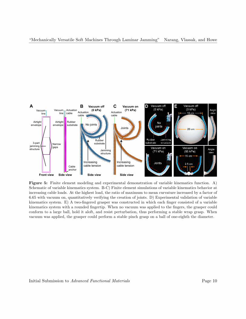
Figure 5: Finite element modeling and experimental demonstration of variable kinematics function. A)Schematic of variable kinematics system. B-C) Finite element simulations of variable kinematics behavior atincreasing cable loads. At the highest load, the ratio of maximum to mean curvature increased by a factor of6.65 with vacuum on, quantitatively verifying the creation of joints. D) Experimental validation of variablekinematics system. E) A two-fingered grasper was constructed in which each finger consisted of a variablekinematics system with a rounded fingertip. When no vacuum was applied to the fingers, the grasper couldconform to a large ball, hold it aloft, and resist perturbation, thus performing a stable wrap grasp. Whenvacuum was applied, the grasper could perform a stable pinch grasp on a ball of one-eighth the diameter.
Initial Submission to Advanced Functional Materials Page 10
“Mechanically Versatile Soft Machines Through Laminar Jamming” Narang, Vlassak, and Howe
around smaller objects[25, 26]; it is challeng-ing to design and fabricate hands capable ofboth. To accomplish the task, we built a two-fingered grasper in which each finger consistedof a cable-actuated variable kinematics systemwith a rounded fingertip. When no vacuum wasapplied and the cables were pulled, the devicecould perform a stable wrap grasp on a ball ofdiameter 20cm; when vacuum was applied first,the device could perform a stable pinch grasp ona ball of one-eighth the diameter (Figure 5E).
To evaluate the stability of the grasps, multi-axis stiffness measurements were conducted anda perturbation test was performed (SI: Func-tions and Applications: Two-FingeredGrasper). Stiffness measurements showed thatthe maximum bending stiffness of a finger in-creased by at least a factor of thirty-two whenvacuum was applied. Simultaneously, the off-axis bending stiffness (i.e., the stiffness along theperpendicular bending axis) increased by a fac-tor of 2.5, and the torsional stiffness increased bya factor of 2.7. Furthermore, perturbation testsdemonstrated that the force required to dislodgethe ball during the pinch grasp increased by atleast a factor of eight when vacuum was applied.
Discussion
Modeling
Earlier studies of laminar jamming exclusivelypredicted the stiffness of jamming structuresduring pre-slip, as well as the first transition load(i.e., the load at which the structures move frompre-slip to the transition regime) [17, 20, 27]. Incontrast, our analytical model predicted the elas-tica, stiffness, energy dissipation, and dampingof two-layer jamming structures during pre-slip,the transition regime, and full-slip, as well as de-
termining both the first transition load and thesecond transition load (i.e., the load at whichthe structures move from the transition regimeto full-slip). Our finite element models of many-layer jamming structures then extended the pre-dictions of the analytical model to structureswith arbitrary numbers of layers. Thus, theanalytical and finite element models completelydescribed the mechanical behavior of jammingstructures over all three phases of deformation.
Together, the models provide designers withan accurate and efficient means to predict themechanical behavior of arbitrary jamming struc-tures. In particular, no models have existed formechanical behavior in the transition regime orfull-slip. To determine how a particular jammingstructure will behave in these phases, designershave had to fabricate and characterize the struc-ture. In our experience, this process requireshours of continuous labor per structure. In con-trast, the analytical model can predict experi-mental behavior for a two-layer jamming struc-ture immediately, and a finite element simulationcan predict experimental behavior for a many-layer structure in less than one hour without su-pervision.
In addition, the functional dependencies ofperformance metrics on design inputs wereextracted for many-layer jamming structures.These relations provide researchers with a rapidmeans to meet arbitrary design requirements.For instance, if the full-slip stiffness of a jam-ming structure must be reduced by a factor offour (e.g., for an orthosis that softens at highloads for user safety), the relations show that thethe number of layers or vacuum pressure can bereduced by a factor of four, or the coefficient offriction can be reduced by a factor of two (TableS1). Likewise, if the full-slip damping of a jam-ming structure must be increased by a factor of
Initial Submission to Advanced Functional Materials Page 11
“Mechanically Versatile Soft Machines Through Laminar Jamming” Narang, Vlassak, and Howe
four (e.g., for a field robot that dampens im-pacts to protect components), then the numberof layers, vacuum pressure, or coefficient of fric-tion can be increased by a factor of four. Notethat vacuum pressure can be controlled on com-mand with a vacuum regulator; thus, full-slipstiffness and damping can be adjusted in real-time. The finite element models can be usedto derive functional dependencies between addi-tional performance metrics and design inputs asdesired.
Useful Functions
Previous studies applied laminar jamming to di-verse applications. However, these studies al-most exclusively used laminar jamming to con-trol stiffness; furthermore, when the jammingstructures were integrated with actuators, thestructures controlled the stiffness of the systemwhile the actuators were continuously powered.We expanded on these capabilities by demon-strating shape-locking and variable kinematics.The former enables soft machines to preservetheir shape after the actuation input is removed,whereas the latter enables them to select be-tween continuous and discrete bending.
Shape-locking illustrates one way in whichlaminar jamming structures can enable soft ma-chines to reversibly emulate traditional rigidrobots. Nearly all traditional robotic armscan navigate to an arbitrary location in theirworkspace and resist static loading. Further-more, some arms have brakes that allow themto resist loading after power is disconnected.Shape-locking endows soft machines with pre-cisely this ability, as it enables them to achievean arbitrary configuration, lock in place, and re-sist static loading, even after disconnecting theactuation input. Soft machines can thus save
power by requiring no control effort to preservetheir shape; furthermore, soft machines withhigh material strain (e.g., McKibben actuators)can be deflated after locking, mitigating the riskof catastrophic rupture.
Variable kinematics comprises a second way inwhich laminar jamming structures can link thebehavior of soft machines and traditional rigidrobots. Specifically, this function can allow softmachines to transform between a compliant statein which they can conform to arbitrary shapes,and a rigid, jointed state in which they can be-have like a serial manipulator. As demonstratedin this study, variable kinematics can enhancethe performance of robotic graspers. More-over, this capability can be useful for any devicewhere both conformability and rigidity are de-sired (e.g., in surgical devices that must traversevasculature, but subsequently apply high forces).
More generally, variable kinematics facilitatesthe modeling, sensing, and control of soft ma-chines. For traditional rigid robots, multi-rigid-body mechanics can describe forward and inversekinematics; on the other hand, soft machines re-quire the mathematical tools of continuum me-chanics, which are generally far more complex.Furthermore, in traditional rigid robots, a smallnumber of sensors can accurately estimate con-figuration; in soft machines, many sensors arerequired. Because modeling and sensing is morecomplex for soft machines, control is inherentlymore difficult[28]. Variable kinematics allowssoft machines to behave like multi-rigid-bodysystems, with rigid links connected by joints.Thus, they can be modeled and sensed like tradi-tional rigid robots, greatly simplifying their con-trol. (It is interesting to note that octopuses usevariable kinematics to simplify control, creatingjoints along their tentacles to facilitate fetchingtasks[29].)
Initial Submission to Advanced Functional Materials Page 12
“Mechanically Versatile Soft Machines Through Laminar Jamming” Narang, Vlassak, and Howe
Limitations
Our modeling and demonstrations have three no-table limitations, each of which can be resolvedas described. First, in our finite element modelsof many-layer jamming structures, the executiontime of the simulations scaled linearly with thenumber of layers; for models of jamming struc-tures with exceptionally high numbers of layers,the time may become prohibitive. Nevertheless,as the numbers of layers increases in a jammingstructure with a fixed total thickness, the struc-ture may be accurately approximated as a singlecrystal with a single slip system. This structurecan be simulated more simply than a multi-layerstructure, reducing execution time (SI: FiniteElement Modeling: Limiting Behavior).
Second, in our shape-locking demonstration,our prototype still required a vacuum source tobe connected after depressurization. Thus, thedevice would be challenging to operate in en-vironments where supporting equipment is un-available. This difficulty could be resolved byusing a one-way valve to maintain vacuum afterthe vacuum input is disconnected.
Third, in our demonstrations, vacuum wasused to actuate the jamming structures. Asa result, the maximum pressure gradient act-ing on the jamming structures was limited tothe absolute ambient pressure, which in turnreduced the maximum load that could be sus-tained by the structures before their stiffness de-clined. This limit may be overcome by usingelectrostatic actuation[27] or elastic actuation,in which the layers are reversibly compressedby an external elastic structure (e.g., a meshenvelope[23] or spring clips (SI: AdditionalConcepts: Spring-Based Jamming)).
Conclusions
This paper demonstrates how the nonlinearstructural phenomenon of laminar jamming canbridge the paradigms of soft robotics and tra-ditional rigid robotics. We have derived ananalytical model for two-layer jamming struc-tures over all major phases of deformation, con-structed highly accurate finite element models ofmany-layer laminar jamming structures, and ex-tracted functional dependencies of major perfor-mance metrics on critical design inputs. We havedemonstrated two novel functions, shape-lockingand variable kinematics, that illustrate how lam-inar jamming can reversibly endow soft machineswith behavior typical of traditional rigid robots.We also built a simple grasper capable of bothpinch grasps and wrap grasps, demonstratinghow laminar jamming can enhance the perfor-mance of real-world soft robotic systems. Col-lectively, our work elucidates the mechanics oflaminar jamming, accelerates the design processof jamming structures, and provides a founda-tion for creating mechanically versatile machinesand structures that cannot simply be categorizedas “soft” or “rigid.”
Experimental Section
The following is an abridged description of the methods usedin this study. For complete detail, see Supporting Informa-tion.
Analytical Modeling
The axial strain fields in each layer of the jamming structurewere approximated as a superposition of a field that variedlinearly with the vertical coordinate and a field that was con-stant with the vertical coordinate. An interfacial displacementvariable was defined. Moment-stress relations and static equi-librium were used to derive governing equations for sections ofthe structure with cohesive interfaces and sections with slippedinterfaces. Boundary conditions were formulated for clampedand free boundaries, and continuity conditions were defined to
Initial Submission to Advanced Functional Materials Page 13

“Mechanically Versatile Soft Machines Through Laminar Jamming” Narang, Vlassak, and Howe
couple cohesive and slipped interfaces. The boundary-valueproblem was then explicitly solved to determine the elastica ofa cantilevered jamming structure with a uniform distributedload in the pre-slip regime, transition regime, and full-slipregime. During the transition regime, the location of the tran-sition between cohesive and slipped interfaces was also deter-mined. The results were then used to derive stiffness, energydissipation, and damping in each regime, as well as criticalloads between the regimes. Dimensionless parameters weredefined to nondimensionalize all results.
Finite Element Modeling
All finite element models were constructed using finite elementsimulation software (ABAQUS 6.14r2, Dassault Systemes, Vil-lacoublay, France). In the finite element models of the two-layer and many-layer jamming structures, each layer was ap-proximated as a 2D plane-strain structure. Pressure equal tovacuum pressure was applied to all outer surfaces, and loadswere subsequently applied. Large-deformation analysis wasenabled, and the interfaces between the layers were defined ascontact surfaces with a penalty friction formulation. A uniformmesh was used consisting of square four-node bilinear plane-strain quadrilateral elements with reduced integration. Eachlayer was meshed with two elements across its thickness.
In the finite element models of the variable kinematics struc-tures, the rubber substrate and each of the jamming structureswas modeled as a homogeneous 2D plane-strain structure. Tosimulate the vacuum-on condition, the elastic modulus of thejamming structure was assigned to that of paper, and to sim-ulate the vacuum-off condition, the modulus was reduced bya factor of n2, with n = 20 to match experimental condi-tions. Cable actuation was approximated as a pure momentload. Large-deformation analysis was enabled. A uniformmesh was used consisting of square four-node bilinear plane-strain quadrilateral hybrid elements with reduced integration.The structure was meshed with four elements across its thick-ness.
Fabrication of Jamming Structures
The jamming structures were fabricated in five distinct steps.1) Sheets of copy paper (HP Ultra White Multipurpose CopyPaper) were cut into strips on a laser cutter (VLS4.60, Univer-sal Laser Systems, Inc., Scottsdale, AZ). 2) An acrylic frameenclosing the strips was cut on the laser cutter. 3) A sheet ofthermoplastic polyurethane (TPU) (American Polyfilm, Inc.,Branford, CT) was formed to the acrylic frame on a vacuumformer (Formech 300XQ, Formech International Limited, Hert-fordshire, UK). 4) The strips of paper and TPU tubing (EldonJames Corp., Denver, CO) were placed into the frame. TheTPU sheet was folded over its contents, and the two sides ofthe sheet were sealed together on a heat press (Powerpress,Fancierstudio, Hayward, CA) at 100◦C, creating a jammingstructure. 5) The end of the structure containing the TPU tub-ing was sandwiched between two conforming aluminum blocks.
The blocks were heated to 171◦C on the heat press, creatinga circumferential seal around the tubing.
Experimental Characterization
Jamming structures were tested on a three-point bending fix-ture in a universal materials testing device (Instron 5566, Illi-nois Tool Works, Norwood, MA). The structures were placedon the fixture and connected to a manual vacuum regulator(EW-07061-30, Cole-Parmer, Vernon Hills, IL) set to the de-sired pressure. The loading anvil of the testing device was low-ered at a rate of 25 mm/min until reaching the desired max-imum displacement. Force and displacement measurementswere simultaneously recorded.
Functions and Applications
All molds were designed using CAD software (Solidworks 2015,Dassault Systemes, Villacoublay, France) and 3D printed us-ing a stereolithography-based printer (Objet30 Scholar, Strata-sys, Ltd., Eden Prairie, MN). For the actuator used in shape-locking demonstrations, a two-part mold was designed, andthe actuator was cast from shore 10A platinum-cure siliconerubber (Dragon Skin 10 Medium, Smooth-On, Inc., Macungie,PA). The actuator and jamming structure were bonded us-ing silicone building sealant (Dow Corning 795, Dow Corning,Midland, MI).
For the substrate used in the variable kinematics demon-strations, a one-part mold was designed with an inserted rod tocreate a channel for an actuation cable. The substrate was castfrom high-stiffness PDMS rubber (Sylgard 184, Dow Corning,Midland, MI). The substrate and three-part jamming struc-ture were again bonded using silicone building sealant. Thecable consisted of braided polyethylene (Hollow Spectra, BHPTackle, Harrington Park, NJ) and was tensioned using a turn-buckle mechanism.
For the fingertips of the fingers in the two-fingered grasper,a two-part mold was designed, and the fingertip was castfrom shore 00-10A silicone rubber (Ecoflex 00-10, Smooth-On,Inc., Macungie, PA). Multi-axis stiffness tests and perturba-tion tests were performed using a digital force gauge (ChatillonDFI10, AMETEK Sensors, Test & Calibration, Berwyn, PA)and custom-built fixtures.
Supporting Information
Supporting Information is available from the Wiley Online Li-brary or from the author.
Acknowledgements
We would like to thank the Harvard Biorobotics Laboratory;the Vlassak Group; the Harvard Biodesign Laboratory; the
Initial Submission to Advanced Functional Materials Page 14

“Mechanically Versatile Soft Machines Through Laminar Jamming” Narang, Vlassak, and Howe
Bertoldi Group; and James Weaver, Ph.D., for their tech-nical advice and assistance. Funding was provided by theNational Science Foundation Graduate Research FellowshipAward 1122374 and the National Science Foundation NationalRobotics Initiative Grant CMMI-1637838.
References
[1] K Suzumori, S Iikura, and H Tanaka. Applyinga flexible actuator to robotic mechanisms. IEEEControl Systems, 12:21–27, 1993.
[2] F Ilievski, AD Mazzeo, RF Shepherd, X Chen,and GM Whitesides. Soft robotics for chemists.Angewandte Chemie, 50:1890–1895, 2011.
[3] OA Araromi, I Gavrilovich, J Shintake, S Ros-set, M Richard, V Gass, and HR Shea. Rollablemultisegment dielectric elastomer minimum en-ergy structures for a deployable microsatellitegripper. IEEE/ASME Transactions on Mecha-tronics, 20:438–446, 2014.
[4] S Shian, K Bertoldi, and D Clarke. Dielectricelastomer based “grippers” for soft robotics. Ad-vanced Materials, 2015.
[5] RV Martinez, JL Branch, CR Fish, L Jin,RF Shepherd, RMD Nunes, Z Suo, andGM Whitesides. Robotic tentacles with three-dimensional mobility based on flexible elas-tomers. Advanced Materials, 25:205–212, 2013.
[6] R Deimel and O Brock. A novel type of com-pliant and underactuated robotic hand for dex-terous grasping. The International Journal ofRobotics Research, 35:161–185, 2016.
[7] MT Tolley, RF Shepherd, B Mosadegh, KC Gal-loway, M Wehner, M Karpelson, RJ Wood, andGM Whitesides. A resilient, untethered robot.Soft Robotics, 1:213–223, 2014.
[8] P Polygerinos, Z Wang, KC Galloway, RJ Wood,and CJ Walsh. Soft robotic glove for combinedassistance and at-home rehabilitation. Roboticsand Autonomous Systems, 73:135–143, 2015.
[9] M Cianchetti, T Ranzani, G Gerboni,T Nanayakkara, K Althoefer, P Dasgupta,and A Menciassi. Soft robotics technologiesto address shortcomings in today’s minimallyinvasive surgery: The STIFF-FLOP approach.Soft Robotics, 1:122–131, 2014.
[10] N Cheng, G Ishigami, S Hawthorne, H Chen,M Hansen, M Telleria, R Playter, and K Iag-nemma. Design and analysis of a soft mobilerobot composed of multiple thermally activatedjoints driven by a single actuator. In 2010 IEEEInternational Conference on Robotics and Au-tomation (ICRA), pages 5207–5212, 2010.
[11] NG Cheng, A Gopinath, L Wang, K Iagnemma,and AE Hosoi. Thermally tunable, self-healingcomposites for soft robotic applications. Macro-molecular Materials and Engineering, 2014.
[12] C Laschi, M Cianchetti, B Mazzolai, L Margheri,M Follador, and P Dario. Soft robot arminspired by the octopus. Advanced Robotics,26:709–727, 2012.
[13] S Seok, CD Onal, K-J Cho, RJ Wood, D Rus,and S Kim. Meshworm: A peristaltic softrobot with antagonistic nickel titanium coil ac-tuators. IEEE/ASME Transactions on Mecha-tronics, 18:1485–1497, 2013.
[14] C Majidi and RJ Wood. Tunable elastic stiffnesswith microconfined magnetorheological domainsat low magnetic field. Applied Physical Letters,97, 2010.
[15] E Brown, N Rodenberg, J Amend, A Mozeika,E Steltz, MR Zakin, H Lipson, and HM Jaeger.Universal robotic gripper based on the jammingof granular material. Proceedings of the NationalAcademy of Sciences, 107:18809–18814, 2010.
[16] M Manti, V Cacucciolo, and M Cianchetti. Stiff-ening in soft robotics. IEEE Robotics & Automa-tion Magazine, 2016.
[17] S Kawamura, T Yamamoto, D Ishida, T Ogata,Y Nakayama, O Tabata, and S Sugiyama. De-velopment of passive elements with variable
Initial Submission to Advanced Functional Materials Page 15
“Mechanically Versatile Soft Machines Through Laminar Jamming” Narang, Vlassak, and Howe
mechanical impedance for wearable robotics.In 2002 IEEE International Conference onRobotics and Automation (ICRA), pages 248–253, 2002.
[18] S Kawamura, K Kanaoka, Y Nakayama, J Jeon,and D Fujimoto. Improvement of passive el-ements for wearable haptic displays. In 2003IEEE International Conference on Robotics andAutomation (ICRA), pages 816–821, 2003.
[19] J Ou, L Yao, D Tauber, J Steimle, R Niiyama,and H Ishii. jamSheets: Thin interfaces withtunable stiffness enabled by layer jamming. In8th International Conference on Tangible, Em-bedded, and Embodied Interaction (TEI), pages65–72, 2014.
[20] M Bureau, T Keller, R Velik, J Perry, and J Ven-eman. Variable stiffness structure for limb at-tachment. In 2011 IEEE International Confer-ence on Rehabilitation Robotics (ICORR), 2011.
[21] YJ Kim, S Cheng, S Kim, and K Iagnemma.A novel layer jamming mechanism with tun-able stiffness capability for minimally inva-sive surgery. IEEE Transactions on Robotics,29:1031–1042, 2013.
[22] V Wall, R Deimel, and O Brock. Selec-tive stiffening of soft actuators based on jam-ming. In 2015 IEEE International Conferenceon Robotics and Automation (ICRA), pages252–257, 2015.
[23] JLC Santiago, IS Godage, P Gonthina, andID Walker. Soft robots and kangaroo tails:modulating compliance in continuum struc-tures through mechanical layer jamming. SoftRobotics, 3:54–63, 2016.
[24] Soft Robotics Inc.http://www.softroboticsinc.com/, 2017. Ac-cessed: 2017-9-1.
[25] LU Odhner, LP Jentoft, MR Claffee, N Cor-son, Y Tenzer, RR Ma, M Buehler, R Ko-hout, RD Howe, and AM Dollar. A compli-ant, underactuated hand for robust manipula-
tion. The International Journal of Robotics Re-search, 33:736–752, 2014.
[26] Barrett Technology, LLC – Products – Bar-rettHand. http://www.barrett.com/products-hand.htm, 2017. Accessed: 2017-9-1.
[27] M Henke and G Gerlach. On a high-potentialvariable-stiffness device. Microsystem Technolo-gies, 20:599–606, 2014.
[28] C Duriez. Control of elastic soft robots based onreal-time finite element method. In 2013 IEEEInternational Conference on Robotics and Au-tomation (ICRA), pages 3982–3987, 2012.
[29] G Sumbre, G Fiorito, T Flash, and B Hochner.Octopuses use a human-like strategy to controlprecise point-to-point arm movements. CurrentBiology, 16:767–772, 2006.
[30] JC Case, EL White, and RK Kramer. Soft ma-terial characterization for robotic applications.Soft Robotics, 2:80–87, 2015.
[31] Tensile properties of paper and paperboard (us-ing constant rate of elongation apparatus). Tech-nical report, TAPPI T494, 2006.
[32] Coefficients of static and kinetic friction of un-coated writing and printing paper by use ofthe horizontal plane method). Technical report,TAPPI T549, 2013.
[33] T Yokoyama and K Nakai. Evaluation of in-plane orthotropic elastic constants of paper andpaperboard. In Conference and Exposition onExperimental and Applied Mechanics, 2007.
[34] Paper characteristics: Fu-jitsu quality laboratory limited.http://www.fujitsu.com/jp/group/fql/en/services/product-quality/analysis/method/paper/, 2017. Ac-cessed: 2017-9-1.
[35] AD Marchese, RK Katzschmann, and D Rus.A recipe for soft fluidic elastomer robots. SoftRobotics, 2:7–25, 2015.
Initial Submission to Advanced Functional Materials Page 16

SI for “Mechanically Versatile Soft Machines Through Laminar Jamming” Narang, Vlassak, and Howe
Initial Submission to Advanced Functional Materials SI Page 1
Supporting Information
Analytical Modeling
Governing Equations
Consider a two-layer jamming structure. Let each layer be approximated as a thin beam
with a width 𝑏, height ℎ, length 𝐿, elastic modulus 𝐸, Poisson’s ratio 𝜈, and coefficient of
friction 𝜇.
Define a coordinate system with the origin located on the left edge of the structure at the
interface between the layers (Figure S1A). Let the 𝑥-axis be horizontal (i.e., along the
length of the undeformed structure), and let the 𝑦-axis be vertical (i.e., along the height of
the undeformed structure).
Let the jamming structure be subject to a pressure gradient 𝑃. In this study, the jamming
structure is actuated by enclosing the layers in an airtight envelope and applying a
vacuum to the envelope. The pressure gradient 𝑃 is equal to the vacuum pressure (i.e., the
pressure in the envelope below ambient pressure). Thus, under standard atmospheric
conditions, 𝑃 has a maximum value of 1 𝑎𝑡𝑚.
Now let the jamming structure be loaded in the transverse direction. As the load
increases, the longitudinal shear stress along the interface between the layers increases.
At some regions of the interface, the longitudinal shear stress may be less than the
maximum frictional stress (i.e., 𝜏𝑓, which is equal to 𝜇𝑃). These regions will remain
cohesive (i.e., points that are initially coincident along the interface will remain
coincident). On the other hand, at other regions of the interface, the longitudinal shear
stress may equal the maximum frictional stress. These regions will slip (i.e., points that
are initially coincident along the interface will move relative to each another), unless a
boundary condition prevents slip from occurring.
We can write governing equations for cohesive sections of the jamming structure (i.e.,
sections of the jamming structure where the interface is cohesive) and slipped sections of
the structure (i.e., sections of the jamming structure where the interface will slip, unless a
boundary condition prevents slip from occurring).
Cohesive Sections
For cohesive sections of the jamming structure, we can write governing equations
by directly using Euler-Bernoulli beam theory. The axial strain fields in the layers
of the jamming structure are
𝜖1(𝑥, 𝑦) = −𝜅(𝑥)𝑦
𝜖2(𝑥, 𝑦) = −𝜅(𝑥)𝑦

SI for “Mechanically Versatile Soft Machines Through Laminar Jamming” Narang, Vlassak, and Howe
Initial Submission to Advanced Functional Materials SI Page 2
where 𝜖1(𝑥, 𝑦) and 𝜖2(𝑥, 𝑦) are the axial strains in the bottom and top layers,
respectively, and 𝜅(𝑥) is the curvature along the interface.
Let us assume the layers are elastic and isotropic. The corresponding stress fields
are
𝜎1(𝑥, 𝑦) = −𝐸𝜅(𝑥)𝑦 (1)
𝜎2(𝑥, 𝑦) = −𝐸𝜅(𝑥)𝑦 (2)
Note that when we later compare analytical results to finite element results, we
substitute the plane-strain modulus �� =𝐸
1−𝜈2 for the elastic modulus, as 𝑏 ≫ ℎ for
the layers of the jamming structure that is investigated (SI: Finite Element
Model: Two-Layer Jamming Structure).
We derive the first governing equation using the relationship between the
resultant moment and the axial stress in the jamming structure (Figure S1B). The
moment-stress relation for a single beam is given by 𝑀(𝑥) = ∫ −𝜎(𝑥, 𝑦)𝑦 𝑑𝑆𝑆
,
where 𝜎(𝑥, 𝑦) is the axial stress and 𝑆 is the cross-section of the beam. For a two-
layer jamming structure,
𝑀(𝑥) = ∫ −𝜎1(𝑥, 𝑦)𝑦 𝑑𝑆1𝑆1
+ ∫ −𝜎2(𝑥, 𝑦)𝑦 𝑑𝑆2𝑆2
(3)
where 𝑆1 and 𝑆2 are the cross-sections of the bottom and top layers, respectively.
Substituting equations (1) and (2),
𝑀(𝑥) = 2𝜅(𝑥)𝐸𝐼 (4)
where 𝐼 is the second moment of area of a cross-section of the top layer about the
interface between the layers (i.e., 𝑏ℎ3
3). Equation (4) is the only governing
equation for cohesive sections of the jamming structure.
Slipped Sections
In slipped sections of the jamming structure, each layer may have a distinct
neutral axis, and the vertical location of each neutral axis may vary in the
horizontal direction. Thus, we can describe the axial strain fields in the bottom
and top layers as
𝜖1(𝑥, 𝑦) = −𝜅(𝑥)𝑦 + 𝐴1(𝑥) (5)
𝜖2(𝑥, 𝑦) = −𝜅(𝑥)𝑦 + 𝐴2(𝑥) (6)
SI for “Mechanically Versatile Soft Machines Through Laminar Jamming” Narang, Vlassak, and Howe
Initial Submission to Advanced Functional Materials SI Page 3
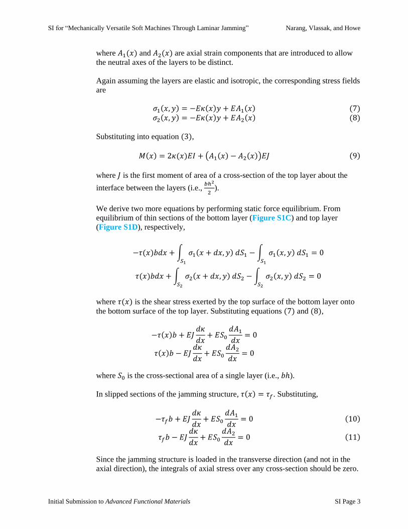
where 𝐴1(𝑥) and 𝐴2(𝑥) are axial strain components that are introduced to allow
the neutral axes of the layers to be distinct.
Again assuming the layers are elastic and isotropic, the corresponding stress fields
are
𝜎1(𝑥, 𝑦) = −𝐸𝜅(𝑥)𝑦 + 𝐸𝐴1(𝑥) (7)
𝜎2(𝑥, 𝑦) = −𝐸𝜅(𝑥)𝑦 + 𝐸𝐴2(𝑥) (8)
Substituting into equation (3),
𝑀(𝑥) = 2𝜅(𝑥)𝐸𝐼 + (𝐴1(𝑥) − 𝐴2(𝑥))𝐸𝐽 (9)
where 𝐽 is the first moment of area of a cross-section of the top layer about the
interface between the layers (i.e., 𝑏ℎ2
2).
We derive two more equations by performing static force equilibrium. From
equilibrium of thin sections of the bottom layer (Figure S1C) and top layer
(Figure S1D), respectively,
−𝜏(𝑥)𝑏𝑑𝑥 + ∫ 𝜎1(𝑥 + 𝑑𝑥, 𝑦) 𝑑𝑆1𝑆1
− ∫ 𝜎1(𝑥, 𝑦) 𝑑𝑆1𝑆1
= 0
𝜏(𝑥)𝑏𝑑𝑥 + ∫ 𝜎2(𝑥 + 𝑑𝑥, 𝑦) 𝑑𝑆2𝑆2
− ∫ 𝜎2(𝑥, 𝑦) 𝑑𝑆2𝑆2
= 0
where 𝜏(𝑥) is the shear stress exerted by the top surface of the bottom layer onto
the bottom surface of the top layer. Substituting equations (7) and (8),
−𝜏(𝑥)𝑏 + 𝐸𝐽𝑑𝜅
𝑑𝑥+ 𝐸𝑆0
𝑑𝐴1
𝑑𝑥= 0
𝜏(𝑥)𝑏 − 𝐸𝐽𝑑𝜅
𝑑𝑥+ 𝐸𝑆0
𝑑𝐴2
𝑑𝑥= 0
where 𝑆0 is the cross-sectional area of a single layer (i.e., 𝑏ℎ).
In slipped sections of the jamming structure, 𝜏(𝑥) = 𝜏𝑓. Substituting,
−𝜏𝑓𝑏 + 𝐸𝐽𝑑𝜅
𝑑𝑥+ 𝐸𝑆0
𝑑𝐴1
𝑑𝑥= 0 (10)
𝜏𝑓𝑏 − 𝐸𝐽𝑑𝜅
𝑑𝑥+ 𝐸𝑆0
𝑑𝐴2
𝑑𝑥= 0 (11)
Since the jamming structure is loaded in the transverse direction (and not in the
axial direction), the integrals of axial stress over any cross-section should be zero.

SI for “Mechanically Versatile Soft Machines Through Laminar Jamming” Narang, Vlassak, and Howe
Initial Submission to Advanced Functional Materials SI Page 4
From equations (7) and (8), we find that 𝐴1(𝑥) + 𝐴2(𝑥) = 0. Thus, equations (9)-(11) can be simplified to
𝑀(𝑥) = 2𝜅(𝑥)𝐸𝐼 + 2𝐴1(𝑥)𝐸𝐽 (12)
−𝜏𝑓𝑏 + 𝐸𝐽𝑑𝜅
𝑑𝑥+ 𝐸𝑆0
𝑑𝐴1
𝑑𝑥= 0 (13)
Equations (12) and (13) are the two governing equations for slipped sections of
the jamming structure.
Strain-Displacement Relations
Slipped Sections
For slipped sections of the jamming structure, it is useful to define variable 𝛿1(𝑥)
as the interfacial displacement for the bottom layer (i.e., the displacement of
points along the top surface of the bottom layer) and variable 𝛿2(𝑥) as the
interfacial displacement for the top layer (i.e., the displacement of points along
the bottom surface of the top layer).
From equations (5) and (6), the axial strain fields at the interface (i.e., at 𝑦 = 0)
simplify to 𝜖1(𝑥) = 𝐴1(𝑥) and 𝜖2(𝑥) = 𝐴2(𝑥). Thus, the interfacial
displacements are related to 𝐴1(𝑥) and 𝐴2(𝑥) by the strain-displacement relations
𝛿1(𝑥) = ∫ 𝐴1(𝑥) 𝑑𝑥 (14)
𝛿2(𝑥) = ∫ 𝐴2(𝑥) 𝑑𝑥 (15)
Boundary Conditions
In practice, a jamming structure may be subject to one of several boundary conditions
along its length (e.g., clamped, pinned, roller-supported, free). We provide clamped and
free boundary conditions that will be relevant for our analysis of a cantilevered jamming
structure. Additional boundary conditions can be readily derived for other physical
scenarios.
Cohesive Sections
Clamped Conditions
Clamped boundary conditions at 𝑥 = 𝑎 in cohesive sections of the
jamming structure are
𝑤(𝑎) = 0 (16)

SI for “Mechanically Versatile Soft Machines Through Laminar Jamming” Narang, Vlassak, and Howe
Initial Submission to Advanced Functional Materials SI Page 5
𝑑𝑤
𝑑𝑥(𝑎) = 0 (17)
where 𝑤(𝑥) is the transverse deflection of the jamming structure.
Slipped Sections
Clamped Conditions
As in cohesive sections, clamped boundary conditions at 𝑥 = 𝑎 in slipped
sections of the jamming structure are
𝑤(𝑎) = 0 (18)
𝑑𝑤
𝑑𝑥(𝑎) = 0 (19)
We can also formulate additional clamped boundary conditions for slipped
sections. At a clamped point, the neutral axes of both layers (i.e., where
𝜖(𝑎, 𝑦) = 0) must be located at the interface (i.e., at 𝑦 = 0). Substituting
into equations (5) and (6), we find the boundary conditions
𝐴1(𝑎) = 0 (20)
𝐴2(𝑎) = 0
In addition, at a clamped point, no interfacial displacements can occur.
Thus, we can also write the boundary conditions
𝛿1(𝑎) = 0 (21)
𝛿2(𝑎) = 0
Free Conditions
For a free boundary at 𝑥 = 𝑏, we know 𝜎1(𝑏, 𝑦) = 𝜎2(𝑏, 𝑦) = 0.
Substituting into equations (7) and (8), we find the boundary condition
𝜅(𝑏) = 0 (22)
Continuity
If a cohesive section and a slipped section of a jamming structure are adjacent,
transverse deflections and slopes must be continuous. Symbolically, if the
sections share a boundary at 𝑥 = 𝑐,
𝑤(𝑐−) = 𝑤(𝑐+) (23) 𝑑𝑤
𝑑𝑥(𝑐−) =
𝑑𝑤
𝑑𝑥(𝑐+) (24)
SI for “Mechanically Versatile Soft Machines Through Laminar Jamming” Narang, Vlassak, and Howe
Initial Submission to Advanced Functional Materials SI Page 6
Explicit Solution
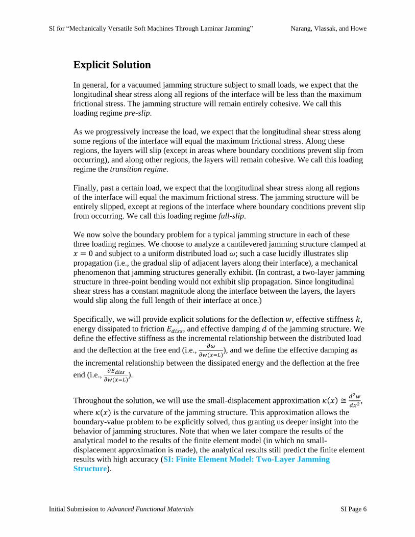
In general, for a vacuumed jamming structure subject to small loads, we expect that the
longitudinal shear stress along all regions of the interface will be less than the maximum
frictional stress. The jamming structure will remain entirely cohesive. We call this
loading regime pre-slip.
As we progressively increase the load, we expect that the longitudinal shear stress along
some regions of the interface will equal the maximum frictional stress. Along these
regions, the layers will slip (except in areas where boundary conditions prevent slip from
occurring), and along other regions, the layers will remain cohesive. We call this loading
regime the transition regime.
Finally, past a certain load, we expect that the longitudinal shear stress along all regions
of the interface will equal the maximum frictional stress. The jamming structure will be
entirely slipped, except at regions of the interface where boundary conditions prevent slip
from occurring. We call this loading regime full-slip.
We now solve the boundary problem for a typical jamming structure in each of these
three loading regimes. We choose to analyze a cantilevered jamming structure clamped at
𝑥 = 0 and subject to a uniform distributed load 𝜔; such a case lucidly illustrates slip
propagation (i.e., the gradual slip of adjacent layers along their interface), a mechanical
phenomenon that jamming structures generally exhibit. (In contrast, a two-layer jamming
structure in three-point bending would not exhibit slip propagation. Since longitudinal
shear stress has a constant magnitude along the interface between the layers, the layers
would slip along the full length of their interface at once.)
Specifically, we will provide explicit solutions for the deflection 𝑤, effective stiffness 𝑘,
energy dissipated to friction 𝐸𝑑𝑖𝑠𝑠, and effective damping 𝑑 of the jamming structure. We
define the effective stiffness as the incremental relationship between the distributed load
and the deflection at the free end (i.e., 𝜕𝜔
𝜕𝑤(𝑥=𝐿)), and we define the effective damping as
the incremental relationship between the dissipated energy and the deflection at the free
end (i.e., 𝜕𝐸𝑑𝑖𝑠𝑠
𝜕𝑤(𝑥=𝐿)).
Throughout the solution, we will use the small-displacement approximation 𝜅(𝑥) ≅𝑑2𝑤
𝑑𝑥2 ,
where 𝜅(𝑥) is the curvature of the jamming structure. This approximation allows the
boundary-value problem to be explicitly solved, thus granting us deeper insight into the
behavior of jamming structures. Note that when we later compare the results of the
analytical model to the results of the finite element model (in which no small-
displacement approximation is made), the analytical results still predict the finite element
results with high accuracy (SI: Finite Element Model: Two-Layer Jamming
Structure).

SI for “Mechanically Versatile Soft Machines Through Laminar Jamming” Narang, Vlassak, and Howe
Initial Submission to Advanced Functional Materials SI Page 7
Resultant Shear and Moment
For a jamming structure clamped at 𝑥 = 0 with a uniform distributed load 𝜔, the
resultant shear is
𝑉(𝑥) = 𝜔(𝐿 − 𝑥) (25)
and the resultant moment is
𝑀(𝑥) = −𝜔𝐿2
2+ 𝜔 (𝐿𝑥 −
𝑥2
2) (26)
Pre-slip Regime
Deflection
During pre-slip, the jamming structure is cohesive. Thus, we can start with
governing equation (4). Substituting equation (26) into equation (4) and
solving for 𝑑2𝑤
𝑑𝑥2 ,
𝑑2𝑤
𝑑𝑥2= −
𝜔𝐿2
4𝐸𝐼+
𝜔𝐿
2𝐸𝐼𝑥 −
𝜔
4𝐸𝐼𝑥2
Integrating twice,
𝑤(𝑥) = −𝜔𝐿2
8𝐸𝐼𝑥2 +
𝜔𝐿
12𝐸𝐼𝑥3 −
𝜔
48𝐸𝐼𝑥4 + 𝐶1𝑥 + 𝐶2 (27)
Applying clamped boundary conditions (18) and (19) at 𝑥 = 0,
𝑤(𝑥) = −𝜔𝐿2
8𝐸𝐼𝑥2 +
𝜔𝐿
12𝐸𝐼𝑥3 −
𝜔
48𝐸𝐼𝑥4
which is a standard result from Euler-Bernoulli beam theory.
Substituting the explicit expression for 𝐼 provided earlier (i.e., 𝐼 =𝑏ℎ3
3),
we find the equivalent expression
𝑤(𝑥) = −3𝜔𝐿2
8𝐸𝑏ℎ3𝑥2 +
𝜔𝐿
4𝐸𝑏ℎ3𝑥3 −
𝜔
16𝐸𝑏ℎ3𝑥4 (28)
Stiffness, Dissipated Energy, and Damping

SI for “Mechanically Versatile Soft Machines Through Laminar Jamming” Narang, Vlassak, and Howe
Initial Submission to Advanced Functional Materials SI Page 8
Substituting equation (28) into the definition of the effective stiffness of
the jamming structure,
𝑘 =16𝐸𝑏ℎ3
3𝐿4(29)
Note that the effective stiffness is constant. Thus, the coefficient of
friction and the vacuum pressure have no effect on the stiffness in the pre-
slip regime.
Since there is no slip in the pre-slip regime, no energy is dissipated to
friction. Thus, the dissipated energy and effective damping are
𝐸𝑑𝑖𝑠𝑠 = 0 (30)
𝑑 = 0 (31)
Transition Regime
From equation (25), the resultant shear is maximum at the clamped end of the
jamming structure and zero at the free end; thus, longitudinal shear stress is also
maximum at the clamped end and zero at the free end. Therefore, we expect that
the layers would begin slipping along their interface near the clamped end, and
that the slipped region would grow until reaching the free end.
Thus, in the transition regime, we can divide the jamming structure into a slipped
section and a cohesive section. Let 𝜒 be the value of 𝑥 where the interface
transitions from slipped to cohesive. We do not know 𝜒 a priori and will solve for
its value.
Slipped Section (𝟎 ≤ 𝒙 ≤ 𝝌)
Deflection
To calculate 𝑤(𝑥) in the slipped section of the jamming structure
in the transition regime, we first find general expressions for
𝐴1(𝑥), 𝛿1(𝑥), and 𝑤(𝑥).
We begin with 𝐴1(𝑥). Solving for 𝑑𝐴1
𝑑𝑥 in governing equation (13)
and integrating,
𝐴1(𝑥) =𝜏𝑓𝑏
𝐸𝑆0𝑥 −
𝐽
𝑆0
𝑑2𝑤
𝑑𝑥2+ 𝐶2 (32)
We proceed to 𝛿1(𝑥). Substituting equation (32) into strain-
displacement relation (14),

SI for “Mechanically Versatile Soft Machines Through Laminar Jamming” Narang, Vlassak, and Howe
Initial Submission to Advanced Functional Materials SI Page 9
𝛿1(𝑥) =𝜏𝑓𝑏
𝐸𝑆0
𝑥2
2 −
𝐽
𝑆0
𝑑𝑤
𝑑𝑥+ 𝐶2𝑥 + 𝐶1 (33)
Finally, we proceed to 𝑤(𝑥). Substituting equation (26) into
governing equation (12) and solving for 𝑑2𝑤
𝑑𝑥2 ,
𝑑2𝑤
𝑑𝑥2= −
𝜔𝐿2
4𝐸𝐼+
𝜔
2𝐸𝐼(𝐿𝑥 −
𝑥2
2) −
𝐽
𝐼𝐴1(𝑥)
Substituting equation (32),
𝑑2𝑤
𝑑𝑥2(1 −
𝐽2
𝑆0𝐼) = −
𝜔𝐿2
4𝐸𝐼+
𝜔
2𝐸𝐼(𝐿𝑥 −
𝑥2
2) −
𝐽
𝐼(
𝜏𝑓𝑏
𝐸𝑆0𝑥 + 𝐶2)
Integrating twice,
𝑤(𝑥) (1 − 𝐽2
𝑆0𝐼) = −
𝜔𝐿2
4𝐸𝐼
𝑥2
2 +
𝜔
2𝐸𝐼(𝐿
𝑥3
6−
𝑥4
24) −
𝐽
𝐼(
𝜏𝑓𝑏
𝐸𝑆0
𝑥3
6+ 𝐶2
𝑥2
2) + 𝐶3𝑥 + 𝐶4 (34)
We can now apply clamped boundary conditions to equations
(32)-(34) to explicitly solve for 𝑤(𝑥). Applying conditions (19)
and (21) to equation (33) at 𝑥 = 0, we find 𝐶1 = 0. Next,
applying conditions (18) and (19) to equation (34) at 𝑥 = 0, we
find 𝐶3 = 𝐶4 = 0. Finally, applying conditions (20) and (21) to
equations (32) and (33), respectively, at 𝑥 = 𝜒,
0 =𝜏𝑓𝑏
𝐸𝑆0𝜒 −
𝐽
𝑆0
𝑑2𝑤
𝑑𝑥2|
𝑥=𝜒
+ 𝐶2 (35)
0 =𝜏𝑓𝑏
𝐸𝑆0
𝜒2
2 −
𝐽
𝑆0
𝑑𝑤
𝑑𝑥|
𝑥=𝜒+ 𝐶2𝜒 (36)
These equations must be consistent with the expressions for 𝑑𝑤
𝑑𝑥|
𝑥=𝜒 and
𝑑2𝑤
𝑑𝑥2 |𝑥=𝜒
that can be derived from equation (34).
Enforcing consistency and solving equations (35) and (36) for 𝐶2
and 𝜒, we find one trivial solution (where 𝜒 = 0) and one non-
trivial solution. The non-trivial solution is
𝐶2 =3(𝜏𝑓𝑏)
2𝐼
4𝜔𝐸𝑆0𝐽−
𝜔𝐿2𝐽
16𝐸𝑆0𝐼−
3𝜏𝑓𝑏𝐿
4𝐸𝑆0
(37)
𝜒 =3𝐿
2−
3𝜏𝑓𝑏𝐼
𝜔𝐽(38)
SI for “Mechanically Versatile Soft Machines Through Laminar Jamming” Narang, Vlassak, and Howe
Initial Submission to Advanced Functional Materials SI Page 10
Substituting equation (37) into equation (34) and solving for
𝑤(𝑥), we find
𝑤(𝑥) =1
1−𝐽2
𝑆0𝐼
((𝜔(𝐿𝐽)2
32𝐸𝑆0𝐼2 +3𝜏𝑓𝑏𝐿𝐽
8𝐸𝑆0𝐼−
3(𝜏𝑓𝑏)2
8𝜔𝐸𝑆0−
𝜔𝐿2
8𝐸𝐼) 𝑥2 + (
𝜔𝐿
12𝐸𝐼−
𝜏𝑓𝑏𝐽
6𝐸𝑆0𝐼) 𝑥3 −
𝜔
48𝐸𝐼𝑥4) (39)
As desired, equation (39) is the deflection in the slipped section of
the jamming structure in the transition regime. Equation (38)
provides the length of the slipped section (i.e., the length of the
slipped region along the interface between the layers) as a function
of the distributed load and the maximum frictional stress.
If we substitute the explicit expressions for 𝐽, 𝐼, and 𝜏𝑓 provided
earlier (i.e., 𝐽 =𝑏ℎ2
2, 𝐼 =
𝑏ℎ3
3, and 𝜏𝑓 = 𝜇𝑃) into equations (38)
and (39) and simplify, we find the equivalent expressions
𝜒 =3𝐿
2−
2𝜇𝑃𝑏ℎ
𝜔(40)
𝑤(𝑥) = (9𝜇𝑃𝐿
4𝐸ℎ2−
3(𝜇𝑃)2𝑏
2𝜔𝐸ℎ−
39𝜔𝐿2
32𝐸𝑏ℎ3) 𝑥2 + (
𝜔𝐿
𝐸𝑏ℎ3−
𝜇𝑃
𝐸ℎ2) 𝑥3 −
𝜔
4𝐸𝑏ℎ3𝑥4 (41)
This form of the expressions shows the exact functional
dependence of the slipped length and the deflection on all critical
design inputs (i.e., dimensions, material properties, the vacuum
pressure, and the distributed load). Note that the slipped length
grows from a minimum value of zero to a maximum value of the
length of the structure. In addition, its growth rate (i.e., 𝑑𝜒
𝑑𝜔) scales
with the vacuum pressure and the inverse square of the distributed
load.
Stiffness, Dissipated Energy, and Damping
We previously defined the effective stiffness k of the jamming
structure as the incremental relationship between the distributed
load and the deflection at the tip. Since equation (41) is only valid
for the slipped section of the jamming structure (i.e., for 0 ≤ 𝑥 ≤𝜒, where 𝜒 < 𝐿), we do not yet know the deflection at the free end.
Thus, we postpone the calculation of 𝑘 to our subsequent
investigation of the cohesive section.
Nevertheless, all the energy dissipated to friction in the transition
regime arises in the slipped section, as no slip occurs in the

SI for “Mechanically Versatile Soft Machines Through Laminar Jamming” Narang, Vlassak, and Howe
Initial Submission to Advanced Functional Materials SI Page 11
cohesive section. Thus, we can calculate the dissipated energy
𝐸𝑑𝑖𝑠𝑠.
We first compute 𝛿1(𝑥) and 𝛿2(𝑥). Substituting equation (37),
equation (41), and the result 𝐶1 = 0 all into equation (33),
𝛿1(𝑥) =1
(1 −𝐽2
𝑆0𝐼)
(36(𝜏𝑓𝑏𝐼)2
− 36𝜔𝜏𝑓𝑏𝐿𝐽𝐼 + 9(𝜔𝐿𝐽)2) 𝑥 + (24𝜔𝜏𝑓𝑏𝐽𝐼 − 12(𝜔𝐽)2𝐿)𝑥2 + 4(𝜔𝐽)2𝑥3
48𝜔𝐸𝑆0𝐽𝐼(42)
From the earlier result 𝐴1(𝑥) + 𝐴2(𝑥) = 0 and the clamped
boundary condition 𝛿2(0) = 0, we find the intuitive result 𝛿2(𝑥) =−𝛿1(𝑥). We can define 𝛿𝑟(𝑥) as the relative displacement between
points that were initially coincident on the interface (i.e., 𝛿1(𝑥) −𝛿2(𝑥)). Thus, 𝛿𝑟(𝑥) = 2𝛿1(𝑥).
The dissipated energy 𝐸𝑑𝑖𝑠𝑠 is the local frictional force per unit
length at the interface, multiplied by the relative interfacial
displacement, integrated over the length of the slipped section.
Symbolically,
𝐸𝑑𝑖𝑠𝑠 = ∫ 𝜏𝑓𝑏𝛿𝑟(𝑥)𝑑𝑥𝜒
0
(43)
Substituting 𝛿𝑟(𝑥),
𝐸𝑑𝑖𝑠𝑠 =1
(1 −𝐽2
𝑆0𝐼)
36(𝜏𝑓𝑏)3
(𝜒𝐼)2 + 4𝜔(𝜏𝑓𝑏𝜒)2
𝐽𝐼(4𝜒 − 9𝐿) + 𝜔2𝜏𝑓𝑏(𝜒𝐽)2(9𝐿2 − 8𝐿𝜒 + 2𝜒2)
48𝜔𝐸𝑆0𝐽𝐼
Substituting the explicit expressions for 𝐼, 𝐽, 𝜏𝑓, and 𝜒, we find the
equivalent expression
𝐸𝑑𝑖𝑠𝑠 =256(𝜇𝑃)5(𝑏ℎ)4 − 768𝜔𝐿(𝜇𝑃)4(𝑏ℎ)3 + 864(𝜔𝐿𝑏ℎ)2(𝜇𝑃)3 − 432(𝜔𝐿)3(𝜇𝑃)2𝑏ℎ + 81(𝜔𝐿)4𝜇𝑃
192𝜔3𝐸ℎ2(44)
This form of the expression shows the exact functional dependence
of the dissipated energy in the transition regime on all critical
design inputs (i.e., dimensions, material properties, the vacuum
pressure, and the distributed load).
Finally, as described earlier, we define the effective damping d as
the incremental relationship between 𝐸𝑑𝑖𝑠𝑠 and the maximum
deflection. From the chain rule, we know that 𝜕𝐸𝑑𝑖𝑠𝑠
𝜕𝑤(𝑥=𝐿)=

SI for “Mechanically Versatile Soft Machines Through Laminar Jamming” Narang, Vlassak, and Howe
Initial Submission to Advanced Functional Materials SI Page 12
𝜕𝐸𝑑𝑖𝑠𝑠
𝜕𝜔
𝜕𝜔
𝜕𝑤(𝑥=𝐿). Simplifying, 𝑑 = 𝑘
𝜕𝐸𝑑𝑖𝑠𝑠
𝜕𝜔. Again, we cannot yet
calculate 𝑑 of the jamming structure in the transition regime, as we
have had to postpone our calculation of 𝑘 to the subsequent
investigation of the cohesive section.
Cohesive Section (𝝌 ≤ 𝒙 ≤ 𝑳):
Deflection
To solve for 𝑤(𝑥) in the cohesive section of the jamming structure
in the transition regime, we may begin with equation (27).
Repeating for clarity,
𝑤(𝑥) = −𝜔𝐿2
8𝐸𝐼𝑥2 +
𝜔𝐿
12𝐸𝐼𝑥3 −
𝜔
48𝐸𝐼𝑥4 + 𝐶1𝑥 + 𝐶2 (45)
Applying continuity boundary conditions (23) and (24) at 𝑥 = 𝜒,
we find 𝐶1 = 0,
𝐶2 =1
𝑆0𝐼 − 𝐽2(
−9𝜔𝐿4𝐽2
256𝐸𝐼+
9𝜏𝑓𝑏𝐿3𝐽
32𝐸−
27(𝜏𝑓𝑏𝐿)2
𝐼
32𝜔𝐸+
9(𝜏𝑓𝑏)3
𝐿𝐼2
8𝜔2𝐸𝐽−
9(𝜏𝑓𝑏)4
𝐼3
16𝜔3𝐸𝐽2)
and
𝑤(𝑥) = −𝜔𝐿2
8𝐸𝐼𝑥2 +
𝜔𝐿
12𝐸𝐼𝑥3 −
𝜔
48𝐸𝐼𝑥4
+1
𝑆0𝐼 − 𝐽2(
−9𝜔𝐿4𝐽2
256𝐸𝐼+
9𝜏𝑓𝑏𝐿3𝐽
32𝐸−
27(𝜏𝑓𝑏𝐿)2
𝐼
32𝜔𝐸+
9(𝜏𝑓𝑏)3
𝐿𝐼2
8𝜔2𝐸𝐽
−9(𝜏𝑓𝑏)
4𝐼3
16𝜔3𝐸𝐽2)
Substituting the explicit expressions for 𝐼, 𝐽, and 𝜏𝑓, we find
𝑤(𝑥) = −3𝜔𝐿2
8𝐸𝑏ℎ3𝑥2 +
𝜔𝐿
4𝐸𝑏ℎ3𝑥3 −
𝜔
16𝐸𝑏ℎ3𝑥4 +
27𝜇𝑃𝐿3
16𝐸ℎ2−
(𝜇𝑃)4𝑏3ℎ
𝜔3𝐸+
3(𝜇𝑃)3𝑏2𝐿
𝜔2𝐸−
27(𝜇𝑃)2𝑏𝐿2
8𝜔𝐸ℎ−
81𝜔𝐿4
256𝐸𝑏ℎ3(46)
Stiffness, Dissipated Energy, and Damping
As equation (46) is valid for the cohesive section of the jamming
structure (i.e., for 𝜒 ≤ 𝑥 ≤ 𝐿), we now know the deflection at the
free end in the transition regime and can calculate the effective
stiffness 𝑘. Substituting equation (46) into the definition of 𝑘,
SI for “Mechanically Versatile Soft Machines Through Laminar Jamming” Narang, Vlassak, and Howe
Initial Submission to Advanced Functional Materials SI Page 13
𝑘 =256𝜔4𝐸𝑏ℎ3
768(𝜇𝑃𝑏ℎ)4 − 1536𝜔𝐿(𝜇𝑃𝑏ℎ)3 + 864(𝜔𝐿𝜇𝑃𝑏ℎ)2 − 129(𝜔𝐿)4(47)
Note that the effective stiffness of the jamming structure in the
transition regime is a function of both the distributed load and the
vacuum pressure.
We can now solve for the effective damping 𝑑 of the jamming
structure in the transition regime as well. Substituting equations
(47) and (44) into the earlier result 𝑑 = 𝑘𝜕𝐸𝑑𝑖𝑠𝑠
𝜕𝜔,
𝑑 =1024(𝜇𝑃𝑏ℎ)5 − 2048𝜔𝐿(𝜇𝑃𝑏ℎ)4 + 1152(𝜔𝐿)2(𝜇𝑃𝑏ℎ)3 − 108(𝜔𝐿)4𝜇𝑃𝑏ℎ
768(𝜇𝑃𝑏ℎ)4 − 1536𝜔𝐿(𝜇𝑃𝑏ℎ)3 + 864(𝜔𝐿𝜇𝑃𝑏ℎ)2 − 129(𝜔𝐿)4(48)
Note that the effective damping of the jamming structure in the
transition regime is a function of both the distributed load and the
vacuum pressure as well.
Full-slip Regime
Deflection
To solve for 𝑤(𝑥) of the jamming structure in the full-slip regime, we may
begin with equation (33), as well as equation (34) after applying clamped
boundary conditions (18) and (19) at 𝑥 = 0. Providing for clarity,
𝐴1(𝑥) =𝜏𝑓𝑏
𝐸𝑆0𝑥 −
𝐽
𝑆0
𝑑2𝑤
𝑑𝑥2+ 𝐶2 (49)
𝑤(𝑥) (1 − 𝐽2
𝑆0𝐼) = −
𝜔𝐿2
4𝐸𝐼
𝑥2
2 +
𝜔
2𝐸𝐼(𝐿
𝑥3
6−
𝑥4
24) −
𝐽
𝐼(
𝜏𝑓𝑏
𝐸𝑆0
𝑥3
6+ 𝐶2
𝑥2
2) (50)
We cannot apply continuity boundary conditions (23) and (24), as the
entire interface has slipped and the value of 𝜒 has now exceeded the length
of the structure. However, we may apply free boundary condition (22) at
𝑥 = 𝐿. Evaluating, we find 𝐶2 =−𝜏𝑓𝑏𝐿
𝐸𝑆0. Substituting into equation (50)
and solving for 𝑤(𝑥),
𝑤(𝑥) =1
1 − 𝐽2
𝑆0𝐼
((𝜏𝑓𝑏𝐿𝐽
2𝐸𝑆0𝐼−
𝜔𝐿2
8𝐸𝐼) 𝑥2 + (
𝜔𝐿
12𝐸𝐼−
𝜏𝑓𝑏𝐽
6𝐸𝑆0𝐼) 𝑥3 −
𝜔
48𝐸𝐼𝑥4) (51)

SI for “Mechanically Versatile Soft Machines Through Laminar Jamming” Narang, Vlassak, and Howe
Initial Submission to Advanced Functional Materials SI Page 14
Substituting the explicit expressions for 𝐼, 𝐽, and 𝜏𝑓, we find the equivalent
expression
𝑤(𝑥) = (3𝜇𝑃𝐿
𝐸ℎ2−
3𝜔𝐿2
2𝐸𝑏ℎ3) 𝑥2 + (
𝜔𝐿
𝐸𝑏ℎ3−
𝜇𝑃
𝐸ℎ2) 𝑥3 −
𝜔
4𝐸𝑏ℎ3𝑥4 (52)
Note that the deflection of the jamming structure in the full-slip regime is
a function of the coefficient of friction and the vacuum pressure. In
contrast, the deflection of a two-layer structure with a frictionless interface
(or equivalently, the deflection of a two-layer structure when no vacuum is
applied) is 𝑤(𝑥) = −3𝜔𝐿2
2𝐸𝑏ℎ3 𝑥2 +𝜔𝐿
𝐸𝑏ℎ3 𝑥3 −𝜔
4𝐸𝑏ℎ3 𝑥4, which depends on
neither the coefficient of friction nor the vacuum pressure.
Stiffness, Dissipated Energy, and Damping
Substituting equation (52) into the definition of the effective stiffness of
the jamming structure,
𝑘 =4𝐸𝑏ℎ3
3𝐿4(53)
Note that the effective stiffness of the jamming structure in the full-slip
regime is constant. In addition, this stiffness is equal to the effective
stiffness of a two-layer structure with a frictionless interface (or
equivalently, the stiffness of a two-layer structure when no vacuum is
applied).
Analogous to the slipped section of the transition regime, to calculate
𝐸𝑑𝑖𝑠𝑠, we first compute 𝛿𝑟(𝑥). We may begin with equation (33).
Repeating for clarity,
𝛿1(𝑥) =𝜏𝑓𝑏
𝐸𝑆0
𝑥2
2 −
𝐽
𝑆0
𝑑𝑤
𝑑𝑥+ 𝐶2𝑥 + 𝐶1
Applying clamped boundary conditions (19) and (21) at 𝑥 = 0, we find
𝐶1 = 0. Substituting equation (52) and the earlier result 𝐶2 =−𝜏𝑓𝑏𝐿
𝐸𝑆0,
𝛿1(𝑥) =1
(1 −𝐽2
𝑆0𝐼)
(3𝜔𝐿2𝐽 − 12𝜏𝑓𝑏𝐿𝐼)𝑥 + (6𝜏𝑓𝑏𝐼 − 3𝜔𝐿𝐽)𝑥2 + 𝜔𝐽𝑥3
12𝐸𝑆0𝐼
As before, 𝛿𝑟(𝑥) = 2𝛿1(𝑥). Substituting into equation (43) with 𝜒 = 𝐿,

SI for “Mechanically Versatile Soft Machines Through Laminar Jamming” Narang, Vlassak, and Howe
Initial Submission to Advanced Functional Materials SI Page 15
𝐸𝑑𝑖𝑠𝑠 =1
(1 −𝐽2
𝑆0𝐼)
3𝜔𝜏𝑓𝑏𝐿4𝐽 − 16(𝜏𝑓𝑏)2
𝐿3𝐼
24𝐸𝑆0𝐼
Substituting the explicit expressions for 𝐼, 𝐽, and 𝜏𝑓, we find the equivalent
expression
𝐸𝑑𝑖𝑠𝑠 =9𝜔𝜇𝑃𝐿4 − 32(𝜇𝑃)2𝑏ℎ𝐿3
12𝐸ℎ2(54)
Note that the dissipated energy in the full-slip regime is a function of both
the distributed load and the vacuum pressure.
Finally, substituting equation (57) into the definition of the effective
damping 𝑑 of the jamming structure, we find
𝑑 = 𝜇𝑃𝑏ℎ (55)
Note that the effective damping of the jamming structure in the full-slip
regime is independent of the distributed load, but scales with the vacuum
pressure. This result suggests that damping may be controlled in a real-
world jamming structure over a continuum of values by forcing the
structure into the full-slip regime and varying vacuum pressure as desired.
This concept is investigated later for many-layer jamming structures (SI:
Additional Concepts: Continuously-Variable Damping).
Transition Loads Between Regimes
Let us define the first transition load 𝜔1 to be the load at which the jamming
structure shifts from the pre-slip regime to the transition regime. The first
transition load can be found by solving equation (40) for 𝜔 when 𝜒 = 0.
Explicitly,
𝜔1 =4𝜇𝑃𝑏ℎ
3𝐿(56)
Let us define the second transition load 𝜔2 to be the load at which the jamming
structure shifts from the transition regime to the full-slip regime. The second
transition load can be found by solving equation (40) for 𝜔 when 𝜒 = 𝐿.
Explicitly,
𝜔2 =4𝜇𝑃𝑏ℎ
𝐿(57)
Summary of Formulae
SI for “Mechanically Versatile Soft Machines Through Laminar Jamming” Narang, Vlassak, and Howe
Initial Submission to Advanced Functional Materials SI Page 16
Equation (28) describes the deflection of the two-layer jamming structure during
the pre-slip regime, and equation (29) describes the effective stiffness of the
structure in this regime. Equations (30) and (31) describe the dissipated energy
and the effective damping, which are zero.
Equations (40), (41), and (46) describe the deflection of the jamming structure
during the transition regime (in both the slipped and cohesive sections of the
structure), and equation (47) describes the effective stiffness of the structure in
this regime. Equations (44) and (48) describe the dissipated energy and the
effective damping, respectively.
Equation (52) describes the deflection of the structure during the full-slip regime,
and equation (53) describes the effective stiffness of the two-layer structure
during this regime. Equations (54) and (55) describe the dissipated energy and
the effective damping, respectively.
Finally, equations (56) and (57) describe the loads at which the jamming
structure shifts between consecutive regimes.
Thus, we have formulated a complete model for the kinematics, stiffness,
dissipated energy, and damping of a two-layer jamming structure over all major
phases of deformation.
Dimensionless Forms
Through nondimensionalization, all the preceding formulae can be dramatically
simplified. We can define dimensionless variables 𝑤∗ =𝑤
𝐿, 𝑥∗ =
𝑥
𝐿, 𝑘∗ =
𝑘
𝐸,
𝐸𝑑𝑖𝑠𝑠∗ =
𝐸𝑑𝑖𝑠𝑠
𝐸𝐿3 , 𝑑∗ =𝑑
𝐸𝐿2, 𝜔∗ =𝜔
𝐸𝐿, 𝜇∗ = 𝜇, 𝑃∗ =
𝑃
𝐸, 𝑏∗ =
𝑏
𝐿, and ℎ∗ =
ℎ
𝐿. We can also
define the composite dimensionless variables 𝛼 = 𝜇∗𝑃∗𝑏∗ℎ∗ and 𝛽 = 𝑏∗ℎ∗3.
Substituting these variables into the formulae, we find the following
dimensionless formulae:
Pre-slip Regime
𝑤∗ = −3𝜔∗
8𝛼∗𝑥∗2 +
𝜔∗
4𝛼∗𝑥∗3 −
𝜔∗
16𝛼∗𝑥∗4
𝑘∗ =16𝛼∗
3
𝐸𝑑𝑖𝑠𝑠∗ = 0
𝑑∗ = 0
Transition Regime

SI for “Mechanically Versatile Soft Machines Through Laminar Jamming” Narang, Vlassak, and Howe
Initial Submission to Advanced Functional Materials SI Page 17
𝑘∗ =256𝜔∗4𝛼∗
768𝛽∗4 − 1536𝜔∗𝛽∗3 + 864𝜔∗2𝛽∗2 − 129𝜔∗4
𝐸𝑑𝑖𝑠𝑠∗ =
256𝛽∗5 − 768𝜔∗𝛽∗4 + 864𝜔∗2𝛽∗3 − 432𝜔∗3𝛽∗2 + 81𝜔∗4𝛽∗
192𝜔∗3𝛼∗
𝑑∗ =1024𝛽∗5 − 2048𝜔∗𝛽∗4 + 1152𝜔∗2𝛽∗3 − 108𝜔∗4𝛽∗
768𝛽∗4 − 1536𝜔∗𝛽∗3 + 864𝜔∗2𝛽∗2 − 129𝜔∗4
Slipped Section
𝜒∗ =3
2−
2𝛽∗
𝜔∗
𝑤∗ = (9𝛽∗
4𝛼∗−
3𝛽∗2
2𝜔∗𝛼∗−
39𝜔∗
32𝛼∗) 𝑥∗2 + (
𝜔∗
𝛼∗−
𝛽∗
𝛼∗) 𝑥∗3 −
𝜔∗
4𝛼∗𝑥∗4
Cohesive Section
𝑤∗ = −3𝜔∗
8𝛼∗𝑥∗2 +
𝜔∗
4𝛼∗𝑥∗3 −
𝜔∗
16𝛼∗𝑥∗4 +
27𝛽∗
16𝛼∗−
𝛽∗4
𝜔3𝛼∗+
3𝛽∗3
𝜔∗2𝛼∗
−27𝛽∗2
8𝜔∗𝛼∗−
81𝜔∗
256𝛼∗
Full-slip Regime
𝑤∗ = (3𝛽∗
𝛼∗−
3𝜔∗
2𝛼∗) 𝑥∗2 + (
𝜔∗
𝛼∗−
𝛽∗
𝛼∗) 𝑥∗3 −
𝜔∗
4𝛼∗𝑥∗4
𝑘∗ =4𝛼∗
3
𝐸𝑑𝑖𝑠𝑠∗ =
9𝜔∗𝛽∗ − 32𝛽∗2
12𝛼∗
𝑑∗ = 𝛽∗
Transition Loads
𝜔1∗ =
4𝛽∗
3
𝜔2∗ = 4𝛽∗

SI for “Mechanically Versatile Soft Machines Through Laminar Jamming” Narang, Vlassak, and Howe
Initial Submission to Advanced Functional Materials SI Page 18
Note that dimensionless deflections are found to depend on at most 4
dimensionless parameters (i.e., 𝜔∗, 𝑥∗, 𝛼∗, and 𝛽∗); dimensionless stiffnesses and
dissipated energies depend on at most 3 parameters (i.e., 𝜔∗, 𝛼∗, and 𝛽∗);
dimensionless damping values depend on at most 2 parameters (i.e., 𝜔∗ and 𝛽∗);
and dimensionless transition loads depend on just 1 parameter (i.e., 𝛽∗).
Case Study
The analytical model was evaluated for an example two-layer jamming structure. Each
layer had dimensions 𝑏 = 50 𝑚𝑚, ℎ = 0.1 𝑚𝑚, and 𝐿 = 250 𝑚𝑚, as well as a
Poisson’s ratio 𝑣 = 0.156 and coefficient of friction 𝜇 = 0.65. These dimensions and
material properties coincided with those of the real-life jamming structures examined
later during experimental characterization (SI: Experimental Characterization:
Characterization Process).
If a two-layer jamming structure with the above properties consisted of compliant
material, it would not slip until the structure exhibited exceptionally large deflections.
Thus, the elastic modulus 𝐸 was set to 6 𝑇𝑃𝑎 in order to illustrate slip over a more
reasonable range of deflection. In addition, as described earlier, the plane-strain modulus
�� =𝐸
1−𝜈2 was substituted for the elastic modulus in the analytical formulae, as 𝑏 ≫ ℎ.
A vacuum pressure 𝑃 = 101 𝑘𝑃𝑎 was imposed, and a uniform distributed load 𝜔 = 7𝑁
𝑚
was applied over 100 equal increments. The elastica (i.e., shape), the deflection at the
free end of the jamming structure, and the dissipated energy were computed for each load
increment.
Curvature Reversal
For a typical cantilever beam under a uniform distributed load, the curvature of the beam
maintains a consistent sign. However, for a two-layer jamming structure, the analytical
model predicts that the curvature reverses (i.e., changes sign) along its length at moderate
loads and higher. Curvature reversal can be seen on close inspection of the elastica in the
case study (Figure 2B).
The analytical model in the transition regime may provide a first explanation of this
counterintuitive phenomenon. Because the net force on any cross section is zero, 𝐴1(𝑥) +𝐴2(𝑥) = 0 for all 𝑥. Furthermore, because the jamming structure is cohesive for 𝜒 ≤ 𝑥 <𝐿, interfacial displacements must be zero at 𝑥 = 𝜒. Thus, positive values of 𝐴1(𝑥) within
the slipped section of the jamming structure (i.e., 0 ≤ 𝑥 ≤ 𝜒) must be balanced by
negative values of 𝐴1(𝑥) elsewhere in the slipped section; likewise, positive values of
𝐴2(𝑥) must be balanced by negative values of 𝐴2(𝑥). Equations (5) and (6) imply a
similar (but not identical) relationship for 𝜅(𝑥).

SI for “Mechanically Versatile Soft Machines Through Laminar Jamming” Narang, Vlassak, and Howe
Initial Submission to Advanced Functional Materials SI Page 19
Curvature reversal was corroborated in detail by finite element models of two-layer
jamming structures, as well as finite element models and experimental observations of
many-layer jamming structures (SI: Finite Element Modeling: Two-Layer Jamming
Structures).
Extending the Model
The analytical modeling procedure for two-layer jamming structures can
be adapted to solve for the deflection of jamming structures with arbitrary numbers of
layers and arbitrary boundary conditions.
Arbitrary Numbers of Layers
Three important results may be simply derived for many-layer jamming
structures. First, the elastica of a vacuumed jamming structure during the pre-slip
regime can be determined by approximating the structure as a cohesive thin beam
and directly using Euler-Bernoulli beam theory to calculate deflection.
Second, as cited in the main text, the bending stiffness of a vacuumed many-layer
jamming structure during the pre-slip regime is a factor of 𝑛2 greater than the
stiffness when no vacuum is applied, where 𝑛 is the number of layers (Reference:
17). This result can be derived from second area moments of inertia. When a
vacuumed jamming structure is in the pre-slip regime, the structure is cohesive,
and the second area moment of inertia of the jamming structure is given by 𝐼 =𝑏(𝑛ℎ)3
12= 𝑛3 𝑏ℎ3
12. When no vacuum is applied to a jamming structure, the layers are
decoupled, and 𝐼 = 𝑛𝑏ℎ3
12. Since bending stiffness is proportional to 𝐼, the stiffness
in the former case is a factor of 𝑛2 greater than that in the latter case.
Third, the first transition load (i.e., the load at which a jamming structure shifts
from the pre-slip regime to the transition regime) for many layer-jamming
structures is given by 𝑉𝑚𝑎𝑥 =2𝜇𝑃𝐴
3, where 𝑉𝑚𝑎𝑥 is the maximum resultant shear at
any cross-section of the beam, which is proportional to the applied load; and 𝐴 is
the total cross-sectional area (i.e., 𝑛𝑏ℎ) (Reference: 27). This result can be
derived from the definition of slip. Slip occurs when the maximum longitudinal
shear stress at an interface equals the maximum possible shear stress. During the
pre-slip regime, the maximum longitudinal shear stress occurs at the innermost
interface and is given by the well-known formula 𝜏𝑚𝑎𝑥 =3𝑉𝑚𝑎𝑥
2𝐴. Furthermore, the
maximum possible shear stress is 𝜇𝑃. Equating the two expressions and solving
for 𝑉𝑚𝑎𝑥, we see 𝑉𝑚𝑎𝑥 =2𝜇𝑃𝐴
3.
Despite the simplicity of deriving the previous three results, solving for the
deformation of a many-layer jamming structure during the transition regime and
full-slip regime is a far greater challenge. This paper has provided detailed

SI for “Mechanically Versatile Soft Machines Through Laminar Jamming” Narang, Vlassak, and Howe
Initial Submission to Advanced Functional Materials SI Page 20
methods for solving for the deformation of a two-layer jamming structure during
these regimes; these methods may be extended to solve the many-layer problem
as well.
For a many-layer jamming structure, strain distributions can again be defined for
each layer as the superposition of a linear strain term and a unique axial strain
term. The moment-stress relation can be used to derive a first governing equation.
Static force equilibrium can then be performed on thin sections of each layer to
derive subsequent governing equations. For the outermost layers, these equations
would be similar to equations (10) and (11) for the two-layer jamming structure;
for inner layers, shear stress would act on both the top and bottom surfaces of the
thin section, producing a second shear stress term.
Whereas slip propagates along one dimension (i.e., along the 𝑥-axis, as defined in
Figure S1A) for a two-layer jamming structure, slip would propagate along two
dimensions (i.e., along the 𝑥- and 𝑦-axes) for a many-layer jamming structure.
Shear stress varies through the thickness of the structure, and slip would occur
along distinct interfaces at disparate loads. Thus, a unique 𝜒 variable would be
required for each interface. Moreover, boundary conditions (20) and (21) would
only be valid at 𝑥 = 𝜒 if 𝜒 corresponded to an interface located along the 𝑥-axis;
for other interfaces, alternative boundary conditions would need to be formulated.
For example, continuity of incremental interfacial displacements and axial strains
may be enforced.
Although the process of solving for the deflection of a many-layer jamming
structure is straightforward, the solution itself may be algebraically taxing.
Furthermore, the analytical solution would only be valid for small deflections.
Thus, numerical solutions (e.g., finite element analysis) may be far more
convenient.
Arbitrary Boundary Conditions
For arbitrary boundary conditions, the direction of shear stress and frictional
stress may change along the length of an interface. Thus, the signs in the
governing equations based on static force equilibrium may vary throughout the
jamming structure. Furthermore, each interface may consist of multiple slipped
and cohesive regions. More than one 𝜒 variable would be necessary for each
interface, along with continuity boundary conditions between adjacent slipped and
cohesive sections of the structure.
Finite Element Modeling
All finite element models were constructed using finite element simulation software (ABAQUS
6.14r2, Dassault Systèmes, Villacoublay, France). Analysis of simulation results was performed
using numerical computing software (MATLAB 2017a, MathWorks, Natick, MA).

SI for “Mechanically Versatile Soft Machines Through Laminar Jamming” Narang, Vlassak, and Howe
Initial Submission to Advanced Functional Materials SI Page 21
Two-Layer Jamming Structures
A finite element model was constructed for a two-layer jamming structure. Each layer
was approximated as a 2D plane-strain structure, and the jamming structure had
dimensions, material properties, vacuum pressure, and distributed load equal to those
specified in the case study for the analytical model of a two-layer jamming structure (SI:
Analytical Modeling: Case Study).
Boundary conditions and loads were also identical to those used in the case study. First,
pressure (equal to the vacuum pressure) was applied to all outer surfaces of the jamming
structure; then, the uniform distributed load was applied as a ramp over 100 equal
increments. Large-deformation analysis was enabled. The interface between the two
layers was chosen to be a contact surface with a penalty friction formulation. The
mitigate undesired simulation of elastic slip, the slip tolerance was set to 5 ∗ 10−5. A
uniform mesh was used that consisted of square four-node bilinear plane-strain
quadrilateral elements with reduced integration (CPE4R). Each layer had two elements
across its thickness. A mesh refinement study was conducted later for many-layer
jamming structures to ensure that a finer mesh was not required (SI: Finite Element
Modeling: Stiffness of Many-Layer Jamming Structures). The elastica, deflection at
the free end, and dissipated energy were extracted at each load increment.
The analytical model predicted finite element results for a two-layer jamming structure
with high accuracy (Figure S2A-C). Elastica were predicted with coefficients of
determination (𝑅2) between 0.9207 and 0.9759. Furthermore, the load-versus-deflection
curve of the structure was predicted with 𝑅2 = 0.9639, and the dissipated-energy-versus-
deflection curve was predicted with 𝑅2 = 0.9977. Note that finite element models of
many-layer jamming structures were later found to predict experimental results with
exceptional accuracy; thus, the analytical model was deemed predictive of real-world
jamming structures as well.
The curvature reversal phenomenon predicted by the analytical model (SI: Analytical
Modeling: Curvature Reversal) was also corroborated by the finite element results
(Figure S2D-E). For the analytical model, curvatures were computed for each of the
analytical elastica in Figure S2A using appropriate first and second derivatives of the
formulae for deflection (SI: Analytical Modeling: Summary of Formulae). For the
finite element model, fourth-order best-fit polynomials were first determined for each of
the finite element elastica in Figure S2A. Curvatures were then computed using
appropriate first and second derivatives of the best-fit polynomials. The analytical
curvature profiles (Figure S2D) were visually predictive of the finite element curvature
profiles (Figure S2E), including the 𝑥-coordinates at which curvature reversal occurred.
Curvature reversal was also observed later for both finite element models and
experimental samples of many-layer jamming structures in three-point bending (Figure
S2F).
Stiffness of Many-Layer Jamming Structures
SI for “Mechanically Versatile Soft Machines Through Laminar Jamming” Narang, Vlassak, and Howe
Initial Submission to Advanced Functional Materials SI Page 22
Finite element models of many-layer jamming structures were constructed according to
the same process used for two-layer jamming structures; however, the structures were
loaded in three-point bending. Rollers (i.e., zero-vertical-displacement boundary
conditions) were applied to two points on the bottom surface, 60 𝑚𝑚 from either side;
the location of these virtual rollers coincided with the location of the rollers used later
during experimental characterization. In addition, to stabilize the finite element model, a
zero-horizontal-displacement boundary condition was applied at the center of the top
surface of the structure.
After applying pressure to all outer surfaces of the jamming structure, a concentrated
transverse displacement was applied to the midpoint of the top surface. The displacement
had a minimum value of 0 𝑚𝑚 and a maximum value of 8 𝑚𝑚 and was applied as a
ramp over 100 equal increments. The displacement range coincided with the range used
later during experimental characterization. The interface between each pair of adjacent
layers was chosen to be a contact surface with a penalty friction formulation. As with the
two-layer jamming structures, a uniform mesh of square elements was used, and each
layer had two elements across its thickness.
A mesh refinement study was conducted to ensure that a finer mesh was not required.
The study was performed for a twenty-layer jamming structure with vacuum pressure
𝑃 = 71.1 𝑘𝑃𝑎 and coefficient of friction μ = 0.65. The number of elements across the
thickness of each layer was varied between one and four (i.e., the areal density of
elements was varied by a factor of sixteen). The one-element simulation did not
converge; however, the two-, three-, and four-element simulations converged
successfully. In each of the converged simulations, the transverse load and maximum
deflection were extracted at each displacement increment. The converged simulations
produced force-versus-maximum-deflection curves that were nearly indistinguishable
(Figure S3A). The mean force difference between the two- and three-element
simulations was 0.050 𝑁 (0.54% of the range of the two-element simulation), and the
mean difference between the two-and four-element simulations was 0.073 𝑁 (0.78% of
the range of the two-element simulation). Thus, it was deemed sufficiently accurate to
mesh each layer with just two elements across its thickness.
The three major design inputs (i.e., the number of layers 𝑛, vacuum pressure 𝑃, and
coefficient of friction 𝜇) were then systematically varied. The quantity 𝑛 was varied from
5 to 20 in increments of 5 (with 𝑃 = 71.1 𝑘𝑃𝑎 and 𝜇 = 0.65); 𝑃 was varied from
23.7 𝑘𝑃𝑎 to 71.1 𝑘𝑃𝑎 in increments of 23.7 𝑘𝑃𝑎 (with 𝑛 = 20 and 𝜇 = 0.65); and 𝜇
was varied from 0.25 to 1 in increments of 0.25 (with 𝑛 = 20 and 𝑃 = 71.1 𝑘𝑃𝑎). For
each set of design inputs, the transverse force and maximum deflection were extracted at
each displacement increment. Recall that the effective stiffness 𝑘 is simply the slope of
the force-versus-maximum-deflection curve.
Aside from providing information about the macroscopic deformation of many-layer
jamming structures, the finite element models also illustrated the microscopic
phenomenon of the slipping of adjacent layers along their interface at high loads (Figure
S3B-C).

SI for “Mechanically Versatile Soft Machines Through Laminar Jamming” Narang, Vlassak, and Howe
Initial Submission to Advanced Functional Materials SI Page 23
Damping of Many-Layer Jamming Structures
In laminar jamming structures, the layers are coupled via dry friction. The relevant
damping phenomenon is Coulomb damping, in which the damping force is independent
of the rate of deformation (as opposed to viscous damping, in which the damping force is
rate-dependent). Even when jamming structures are loaded quasi-statically, energy is still
dissipated. Thus, finite element models of jamming structures subject to static loading are
sufficient to characterize damping, and dynamic simulations are not required.
If interfacial velocities (i.e., the velocities at which adjacent layers slip) were high, the
damping force could theoretically become rate-dependent. However, from the second
term of equation (33) in SI: Analytical Modeling: Explicit Solution, interfacial
displacements are observed to scale with ℎ
𝐿 times the transverse deflection, where ℎ is the
thickness of a layer and 𝐿 is the length. In the jamming structures analyzed in the paper, ℎ
is smaller than 𝐿 by four orders of magnitude; thus, interfacial velocities are negligible
unless transverse velocities are exceptionally high.
The finite element models to analyze damping were built according to the same process
as the finite element models to analyze stiffness. However, after the maximum input
displacement of 8 𝑚𝑚 was applied, the transverse load was reduced to 0 𝑁 over 100
equal increments. The force-versus-maximum-deflection curves then illustrated
hysteresis, and the area under the curves depicted the energy dissipated over the loading
cycle (Figure S4).
Recall that the effective damping 𝑑 is simply the dissipated energy per unit deflection.
The quantity 𝑑 was not explicitly calculated, but can easily be determined. For each point
on the force-versus-maximum-deflection curve, an elastic unloading line can be drawn
(with a slope equal to that of the pre-slip loading line), and the area under the resulting
curve can be computed. This area is the dissipated energy at that particular deflection.
After performing this procedure for all points, the dissipated energy can then be plotted
against deflection. The value of 𝑑 is the slope of this curve.
Functional Dependencies
The finite element simulations for the many-layer jamming structures were rerun over an
extended displacement range (from 0 𝑚𝑚 to 16 𝑚𝑚 over 400 equal increments) to
ensure that all structures entered the full-slip regime, allowing accurate measurement of
full-slip stiffness and damping. Furthermore, the simulations were executed for larger
sets of the design inputs to provide more data points for determining functional
dependence. The numbers of layers examined were 2, 5, 7, 10, 12, 13, 15, 17, 18, and 20;
the vacuum pressures were 0.34, 11.9, 23.7, 35.6, 47.4, 59.3, 71.1, 83.0, 94.8, and
101.1 𝑘𝑃𝑎; and the coefficients of friction were
0.1, 0.2, 0.25, 0.3, 0.4, 0.5, 0.6, 0.7, 0.75, and 0.8.

SI for “Mechanically Versatile Soft Machines Through Laminar Jamming” Narang, Vlassak, and Howe
Initial Submission to Advanced Functional Materials SI Page 24
For each simulation, best-fit lines were fit to the first 1% and the last 1% of the force-
versus-maximum-deflection curve. The slope of the former line approximated the
effective stiffness 𝑘 during pre-slip, whereas the slope of the latter line approximated 𝑘
during full-slip. A best-fit line was then fit to the last 1% of the dissipated-energy-versus-
maximum-deflection curve. The slope of this line approximated the effective damping 𝑑
during full-slip. (Recall that 𝑑 during pre-slip is simply 0).
For each design input (e.g., number of layers), each performance metric (e.g., pre-slip
stiffness) was plotted against the values of the design input (e.g., 2 layers, 5 layers, 7
layers, etc.). Based on the formulae derived in the analytical model for two-layer
jamming structures, it was hypothesized that the performance metrics for many-layer
jamming structures had polynomial dependence on the design inputs. Thus, best-fit
polynomials were fit to each plot; however, the appropriate order for each polynomial
needed to be determined.
Best-fit polynomials from zero- to fourth-order were tested on each plot, and the root-
mean-square error 𝑒𝑟𝑚𝑠 was computed for each polynomial. From physical reasoning,
pre-slip stiffness should be unaffected by the coefficient of friction 𝜇 and the vacuum
pressure 𝑃, as jamming structures are cohesive in pre-slip; thus, the pre-slip stiffness
should have zero-order dependence on 𝜇 and 𝑃. When zero-order polynomials (i.e., flat
lines) were fit to the pre-slip stiffness plots for 𝜇 and 𝑃, it was found that 𝑒𝑟𝑚𝑠 ≅
0.0070𝑁
𝑚𝑚. This value quantified numerical noise in the finite element simulations and
was used as the cutoff for determining the appropriate order of the best-fit polynomial for
the other stiffness plots. Specifically, for a given pre-slip or full-slip stiffness plot, the
lowest-order best-fit polynomial for which 𝑒𝑟𝑚𝑠 ≤ 0.0070𝑁
𝑚𝑚 was determined to be the
appropriate polynomial.
For the full-slip damping plots, dimensional analysis suggested that the 𝑒𝑟𝑚𝑠 threshold
should be multiplied by a characteristic length in order to exhibit the correct units (i.e.,
[𝑁]). As the layers in a jamming structure slip in the direction of their length, the length
𝐿 = 250 𝑚𝑚 was chosen as the characteristic length, and 𝑒𝑟𝑚𝑠 ≅ 0.0070𝑁
𝑚𝑚∗
250 𝑚𝑚 = 1.8 𝑁 was used as the cutoff for determining the appropriate order of the
best-fit polynomial for the damping plots.
The polynomial orders were then tabulated to assess functional dependencies (Table S1).
As expected, pre-slip and full-slip stiffness scaled with 𝑛3and 𝑛, respectively, where 𝑛 is
the number of layers. Full-slip stiffness also scaled with 𝑃 and 𝜇2. In contrast, the
analytical model predicted that the full-slip stiffness of a two-layer jamming structure
was independent of 𝑃 and 𝜇. The dependence of full-slip stiffness on these quantities in
the finite element model is likely a result of contact pressure distributions arising from
the concentrated load and roller supports.
Full-slip damping scaled with 𝑛, 𝑃, and 𝜇. Damping should scale with the number of
interfaces, which in turn scales with 𝑛; furthermore, damping should scale with the
frictional stress at the interfaces, which again is equal to 𝜇𝑃 everywhere during full-slip.

SI for “Mechanically Versatile Soft Machines Through Laminar Jamming” Narang, Vlassak, and Howe
Initial Submission to Advanced Functional Materials SI Page 25
Thus, these scaling relationships are also physically reasonable. Note that the scaling of
full-slip damping with 𝑃 and 𝜇 was also predicted by the analytical model for a two-layer
jamming structure.
For practical applications, one final functional dependence is critical: the dependence of
the first transition load for a many-layer jamming structure (i.e., the load at which the
jamming structure moves from the pre-slip regime to the transition regime) on the design
inputs. However, finite element analysis was not necessary to determine this dependence;
as described earlier, the first transition load can be accurately predicted by Euler-
Bernoulli beam theory and scales with 𝑛, 𝑃, and 𝜇 (SI: Analytical Modeling: Extending
the Model). Note that the scaling of this load with 𝑃 and 𝜇 was predicted by the
analytical model for a two-layer jamming structure as well.
Limiting Behavior
For practical applications, the limiting behavior of jamming structures may be useful to
examine. Consider an application in which the bending stiffness ratio between the
jammed and unjammed states must be maximized (e.g., for a splint that must gently
conform to the shape of a limb and then stiffen to immobilize a joint). This goal can be
accomplished by constructing the layers out of exceptionally thin material (e.g., metal
foil) and stacking as many layers as possible within the total allowable height 𝐻. When
the structure is unjammed, the stiffness will be negligible, as the layers are thin and
flexible. When the structure is jammed, the stiffness will be equal to that of a cohesive
metal structure of height 𝐻.
Nevertheless, such a configuration may have adverse consequences. If the structure is
jammed and unintentionally forced into the full-slip regime (e.g., upon a collision), the
structure will then exhibit a stiffness approximately equal to its unjammed stiffness;
because the unjammed stiffness is negligible, the structure will yield catastrophically if
the load is maintained. Obtaining accurate predictions of the load-deformation curve
during the transition regime and full-slip may help designers avoid such consequences.
Unfortunately, many-layer finite element simulations can be computationally expensive
when the number of layers (and in turn, the number of contact interactions) are
particularly large.
One solution would be to approximate the system by the limiting case in which the layers
of the jamming structure are infinitesimally thin, and an infinite number of layers are
stacked within the height 𝐻. In other words, the structure is approximated as a
continuum. The structure may then be modeled as a single crystal with a single slip
system, with slip planes parallel to the 𝑥𝑧-plane and the slip direction parallel to the 𝑥-
axis. The structure may then be computationally modeled using existing finite element
packages for crystal plasticity.
Variable Kinematics
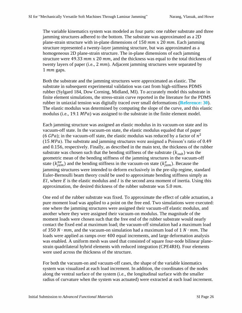
SI for “Mechanically Versatile Soft Machines Through Laminar Jamming” Narang, Vlassak, and Howe
Initial Submission to Advanced Functional Materials SI Page 26
The variable kinematics system was modeled as four parts: one rubber substrate and three
jamming structures adhered to the bottom. The substrate was approximated as a 2D
plane-strain structure with in-plane dimensions of 150 𝑚𝑚 x 20 𝑚𝑚. Each jamming
structure represented a twenty-layer jamming structure, but was approximated as a
homogeneous 2D plane-strain structure. The in-plane dimensions of each jamming
structure were 49.33 𝑚𝑚 x 20 𝑚𝑚, and the thickness was equal to the total thickness of
twenty layers of paper (i.e., 2 𝑚𝑚). Adjacent jamming structures were separated by
1 𝑚𝑚 gaps.
Both the substrate and the jamming structures were approximated as elastic. The
substrate in subsequent experimental validation was cast from high-stiffness PDMS
rubber (Sylgard 184, Dow Corning, Midland, MI). To accurately model this substrate in
finite element simulations, the stress-strain curve reported in the literature for the PDMS
rubber in uniaxial tension was digitally traced over small deformations (Reference: 30).
The elastic modulus was determined by computing the slope of the curve, and this elastic
modulus (i.e., 19.1 𝑀𝑃𝑎) was assigned to the substrate in the finite element model.
Each jamming structure was assigned an elastic modulus in its vacuum-on state and its
vacuum-off state. In the vacuum-on state, the elastic modulus equaled that of paper
(6 𝐺𝑃𝑎); in the vacuum-off state, the elastic modulus was reduced by a factor of 𝑛2
(15 𝑀𝑃𝑎). The substrate and jamming structures were assigned a Poisson’s ratio of 0.49
and 0.156, respectively. Finally, as described in the main text, the thickness of the rubber
substrate was chosen such that the bending stiffness of the substrate (𝑘𝑠𝑢𝑏) was the
geometric mean of the bending stiffness of the jamming structures in the vacuum-off
state (𝑘𝑗𝑎𝑚𝑛𝑣 ) and the bending stiffness in the vacuum-on state (𝑘𝑗𝑎𝑚
𝑣 ). Because the
jamming structures were intended to deform exclusively in the pre-slip regime, standard
Euler-Bernoulli beam theory could be used to approximate bending stiffness simply as
𝐸𝐼, where 𝐸 is the elastic modulus and 𝐼 is the second area moment of inertia. Using this
approximation, the desired thickness of the rubber substrate was 5.0 𝑚𝑚.
One end of the rubber substrate was fixed. To approximate the effect of cable actuation, a
pure moment load was applied to a point on the free end. Two simulations were executed:
one where the jamming structures were assigned their vacuum-off elastic modulus, and
another where they were assigned their vacuum-on modulus. The magnitude of the
moment loads were chosen such that the free end of the rubber substrate would nearly
contact the fixed end at maximum load; the vacuum-off simulation had a maximum load
of 350 𝑁 ∙ 𝑚𝑚, and the vacuum-on simulation had a maximum load of 1 𝑁 ∙ 𝑚𝑚. The
loads were applied as ramps over 400 equal increments, and large deformation analysis
was enabled. A uniform mesh was used that consisted of square four-node bilinear plane-
strain quadrilateral hybrid elements with reduced integration (CPE4RH). Four elements
were used across the thickness of the structure.
For both the vacuum-on and vacuum-off cases, the shape of the variable kinematics
system was visualized at each load increment. In addition, the coordinates of the nodes
along the ventral surface of the system (i.e., the longitudinal surface with the smaller
radius of curvature when the system was actuated) were extracted at each load increment.

SI for “Mechanically Versatile Soft Machines Through Laminar Jamming” Narang, Vlassak, and Howe
Initial Submission to Advanced Functional Materials SI Page 27
The exact local curvatures were then calculated along the surface using appropriate first
and second derivatives of the coordinates.
Experimental Characterization
Fabrication Process
The many-layer jamming structures used in experimental characterization consisted of
three parts: strips of copy paper (HP Ultra White Multipurpose Copy Paper), an envelope
of thermoplastic polyurethane with a thickness of 0.038 𝑚𝑚 (American Polyfilm, Inc.,
Branford, CT), and thermoplastic polyurethane tubing with an outer diameter of 3 𝑚𝑚
(Eldon James Corp., Denver, CO).
The fabrication process for the laminar jamming samples consisted of five major steps
(Figure S4). First, the strips of copy paper were manufactured. Sheets of copy paper
were placed on a laser cutter (VLS4.60, Universal Laser Systems, Inc., Scottsdale, AZ),
and strips were cut along the machine direction of the paper (i.e., the long axis) (Figure
S4A).
Next, the thermoplastic polyurethane (TPU) envelope was created. A frame was cut on
the laser cutter from acrylic plastic (Figure S4B); this frame defined the region of the
TPU sheet that would be sealed in a later step. Since the TPU sheet was intended to form
an envelope around the paper strips and TPU tubing, the shape of the frame comprised a
close perimeter around these contents. Furthermore, since the frame would be in contact
with hot elements in subsequent steps, it was coated with polytetrafluoroethylene (PTFE)
tape to prevent adherence.
The TPU sheet was then formed to the acrylic frame on a vacuum former (Formech
300XQ, Formech International Limited, Hertfordshire, United Kingdom) to create a
pocket in which to place the paper and tubing (Figure S4C). After placing the paper and
tubing into the pocket, the sheet of TPU was folded once upon itself to enclose the pocket
(Figure S4D). The TPU sheet was then covered temporarily with a PTFE sheet and heat-
sealed using a one-sided heat press (Powerpress, Fancierstudio, Hayward, CA) at 100 °𝐶.
Since the heat conduction to the TPU was greatest through the acrylic frame, only the
region of the TPU sheet in contact with the frame was sealed, forming an envelope.
To prevent leakage of air into the envelope, another step was performed to improve the
bond between the TPU envelope and the TPU tubing. A block of aluminum-6061 was
machined with a circular channel through its center, with the diameter of the channel
equal to the diameter of the tubing. The block was then sawed in half through the
channel, and each half was placed on either side of the tubing, sandwiching the tubing
between the two sides of the TPU envelope (Figure S4E). The assembly was then
covered temporarily with a PTFE sheet and heat-sealed at 171 °𝐶. Since only the
aluminum blocks were in contact with the heating element of the heat press, only the
region of the TPU envelope between the blocks was sealed. Thus, a circumferential seal

SI for “Mechanically Versatile Soft Machines Through Laminar Jamming” Narang, Vlassak, and Howe
Initial Submission to Advanced Functional Materials SI Page 28
of the TPU envelope onto the tubing was achieved. The jamming envelope was then
trimmed to its final form (Figure S4F).
Repeatability Analysis
Five twenty-layer jamming structures were fabricated. Each sample was placed in a
universal materials testing device (Instron 5566, Illinois Tool Works, Norwood, MA) and
centered on a static three-point bending fixture (Instron 2810-400) with the supporting
anvils (10 𝑚𝑚 diameter) set 130 𝑚𝑚 apart (Figure S5A).
Vacuum pressure was controlled using a manual vacuum regulator (EW-07061-30, Cole-
Parmer, Vernon Hills, IL). The TPU tubing in each sample was connected to the
regulator via highly flexible polyurethane tubing in order to mitigate parasitic loading of
the sample by the rigid regulator. Prior to each test, a vacuum pressure of 68 ± 1.7 𝑘𝑃𝑎
was applied, and a roller was used to remove residual air pockets from the sample.
The loading anvil (10 𝑚𝑚 diameter) was attached to a 100 𝑁 load cell (Instron 2525-
807) and lowered at a rate of 5𝑚𝑚
𝑚𝑖𝑛 until contacting the sample. When the load cell
measured a value of 0.010 𝑁, the transverse force and displacement of the loading anvil
began to be recorded. The anvil was then lowered at a rate of 25𝑚𝑚
𝑚𝑖𝑛 until reaching a
maximum displacement of 8 𝑚𝑚. Tests were conducted at approximately 20% relative
humidity. After each test, the sample was disconnected from the regulator and gently
flexed multiple times to accelerate its return to ambient pressure. Each sample was tested
ten consecutive times.
Occasionally, the loading anvil initially contacted the jamming structure at protruding
corners of the seam of its polyurethane envelope; this initial contact caused the materials
testing device to undesirably begin measuring force and deflection prior to contacting the
bulk of the jamming structure. To discard measurements of the corners of the envelope,
we neglected data collected before a small initial force threshold of 0.050 𝑁 was reached,
and we defined zero deflection as the deflection at this threshold. This procedure was
always implemented, except for cases in which the force range during a test was
comparable to 0.050 𝑁 (e.g., for five-layer samples in later experimental
characterization). No further filtering or smoothing was performed on the raw data.
For each sample, transverse force was plotted against maximum deflection for all ten
trials. A mean curve was generated, and standard deviations were computed at each point
on the mean curve (Figure S5B-F). The maximum standard deviation at any deflection
was 0.2516 𝑁, which constituted 2.881% of the range of the mean curve for that sample.
Thus, the mechanical behavior of the structures was highly repeatable from trial to trial,
indicating that fatigue was negligible over the examined range of forces and deflections.
The mean curves of all five samples were then aggregated, and a mean curve of the mean
curves was generated (Figure S5G). The maximum standard deviation at any deflection
was 0.1233 𝑁, which constituted 1.414% of the range of the curve. Thus, the mechanical

SI for “Mechanically Versatile Soft Machines Through Laminar Jamming” Narang, Vlassak, and Howe
Initial Submission to Advanced Functional Materials SI Page 29
behavior of the structures was also highly repeatable from sample to sample,
demonstrating that the fabrication process was sufficiently precise. Together, the high
trial-to-trial and sample-to-sample repeatability of the jamming structures showed that
many samples and trials were not required in order to collect statistically representative
data during experimental characterization.
Materials Testing
To provide a fair comparison between experimental and finite element results for many-
layer jamming structures, the elastic modulus 𝐸 and coefficient of friction 𝜇 of the copy
paper used in the jamming samples were experimentally measured; these values were
then used as material properties of the layers in the finite element simulations. The elastic
modulus was measured to be approximately 6 𝐺𝑃𝑎, and the coefficient of friction was
measured to be approximately 0.65. Both properties were measured according to
methods outlined in international paper testing standards (References: 31, 32), and the
values fell within the ranges reported in literature (References: 33, 34). The Poisson’s
ratio of the copy paper was challenging to measure; thus, a literature value of 0.156 was
used instead (Reference: 33).
Stiffness Characterization Process
The stiffness characterization tests were identical to those conducted for the repeatability
analysis (SI: Experimental Characterization: Repeatability Analysis). However,
fewer samples were tested and fewer trials were executed, as the repeatability analysis
showed that many samples and trials were unnecessary. When conducting the tests for the
effect of number of layers on stiffness, three samples were fabricated for each number of
layers (i.e., three five-layer samples, three ten-layer samples, etc.), and each sample was
tested four times at a constant vacuum pressure of 71.1 ± 1.7 𝑘𝑃𝑎. When conducting the
tests for the effect of vacuum pressure, three twenty-layer samples were made in total,
and each sample was tested four times at vacuum pressures of 0, 23.7 ± 1.7, 47.4 ± 1.7, and 71.1 ± 1.7 𝑘𝑃𝑎. No tests were conducted for the effect of coefficient of friction, as
this property could not be precisely varied experimentally.
For each testing group, transverse force was plotted against maximum deflection for all
trials. Recall that the effective stiffness 𝑘 of a jamming structure in three-point bending is
equal to the slope of the force-versus-maximum-deflection curve. Again, mean curves
were generated, and standard deviations were computed at each point on the mean curve.
Damping Characterization Process
To evaluate finite element predictions for how major design inputs affected the damping
of many-layer jamming structures, the damping of jamming structures was
experimentally characterized as well. The tests were identical to those conducted for the
stiffness characterization. However, after the loading anvil reached its maximum
displacement of 8 𝑚𝑚, it was then retracted at a rate of 25𝑚𝑚
𝑚𝑖𝑛 until returning to its

SI for “Mechanically Versatile Soft Machines Through Laminar Jamming” Narang, Vlassak, and Howe
Initial Submission to Advanced Functional Materials SI Page 30
original position of 0 𝑚𝑚. The transverse force and displacement experienced by the
loading anvil continued to be recorded during its retraction. Thus, the behavior of the
jamming structures was measured both during loading and unloading.
Due to the extreme similarity of the damping characterization tests to the stiffness
characterization tests, a minimal number of samples were tested, and a minimal number
of trials were conducted. When conducting the tests for the effect of number of layers on
damping, one sample was fabricated for each number of layers, and each sample was
tested once at a constant vacuum pressure of 71.1 ± 1.7𝑘𝑃𝑎. When conducting the tests
for the effect of vacuum pressure, one twenty-layer sample was made, and the sample
was tested once at vacuum pressures of 0, 23.7 ± 1.7, 47.4 ± 1.7, and 71.1 ± 1.7 𝑘𝑃𝑎.
For each test, transverse force was plotted against maximum deflection for all trials. The
unloading of the sample during each test allowed the hysteresis curve to be observed. The
area under each hysteresis curve depicted the energy dissipated during the loading cycle,
and the effective damping 𝑑 was simply the energy dissipated per unit deflection. Finite
element results for many-layer jamming structures accurately predicted experimental
results (Figure S6). Thus, finite element simulations were not only able to predict the
stiffness of many-layer jamming structures, but also their damping behavior.
Functions and Applications
All molds for the subsequent demonstrations were designed using CAD software (SolidWorks
2015, Dassault Systèmes, Villacoublay, France) and 3D printed using a stereolithography-based
printer (Objet30 Scholar, Stratasys, Ltd., Eden Prairie, MN).
Shape-Locking
A soft pneumatic bending actuator was designed and fabricated based on previous
literature (References: 2, 35). The top of the actuator (i.e., the inflatable chambers) was
cast using a two-part mold, whereas the bottom (i.e., a thick, flat layer to promote
bending rather than extension) was cast using a one-part mold. All parts were cast from
shore 10A platinum-cure silicone rubber (Dragon Skin 10 Medium, Smooth-On, Inc.,
Macungie, PA). A twenty-layer jamming structure was then designed and fabricated
using the techniques described earlier (SI: Experimental Characterization:
Fabrication Process). The structure spanned the ventral surface of the actuator (i.e., the
longitudinal surface with the smaller radius of curvature when the actuator was
pressurized). Finally, the actuator and jamming structure were bonded using silicone
building sealant (Dow Corning 795, Dow Corning, Midland, MI).
The actuator and jamming structure were connected to pressure and vacuum inputs,
respectively. The pressure source was regulated by a digital pressure regulator (ITV1031,
SMC Pneumatics, Yorba Linda, CA), whereas the vacuum source was regulated by the
device used in experimental characterization. The output from each of the regulators
passed through two miniature pneumatic solenoid valves (V2 Valves, Parker Hannifin,

SI for “Mechanically Versatile Soft Machines Through Laminar Jamming” Narang, Vlassak, and Howe
Initial Submission to Advanced Functional Materials SI Page 31
Hollis, NH) before entering the actuator and jamming structure. The valves were
controlled by pushbuttons and enabled the actuator and jamming structure to each have
three states: a pressurizing (or vacuuming) state, a hold state where the internal pressure
(or vacuum) is preserved, and a depressurizing (or vacuum-relieving) state.
The actuator was pressurized to 16 𝑘𝑃𝑎, and a photograph was taken perpendicular to the
bending plane. Two tests were then conducted. In the first test, the actuator was
depressurized to 0 𝑘𝑃𝑎. In the second test, a vacuum of 85 𝑘𝑃𝑎 was first applied to the
jamming structure, and the actuator was then depressurized to 0 𝑘𝑃𝑎. A photograph was
again taken once the system came to rest.
For each photograph, the arc of the ventral surface of the shape-locking system was
digitally traced. The data points comprising each arc were then interpolated over 100
equally spaced points. The coefficient of determination (𝑅2) value was computed
between the two interpolated arcs.
Variable Kinematics
The substrate of the variable kinematics system was fabricated according to the same
process used for the actuator component of the shape-locking system. However, the
substrate was cast using a one-part mold with an inserted hexagonal rod, which created a
channel to route a cable; furthermore, the substrate was cast from high-stiffness PDMS
rubber (Sylgard 184, Dow Corning, Midland, MI). The jamming structure was also
designed and fabricated according to the techniques described earlier, but with three
distinct stacks of twenty strips separated by 1 𝑚𝑚 gaps within the TPU envelope. The
jamming structure and rubber substrate were again bonded with silicone building sealant
(Dow Corning 795, Dow Corning, Midland, MI).
Braided polyethylene cable (Hollow Spectra, BHP Tackle, Harrington Park, NJ) was then
routed through the channel in the substrate. The cable was tied at one end to a turnbuckle
and at the other end to a small washer. During testing, the turnbuckles were manually
twisted, which pulled the cable, compressed the washer against the end of the variable
kinematics structure, and induced bending.
Two-Fingered Grasper
Each fingertip in the two-fingered grasper had a cylindrical surface with a radius of
5 𝑚𝑚. The fingertips were cast using a two-part mold according to the same process used
for the shape-locking actuator and variable-kinematics substrate; however, the fingertips
were cast from shore 00-10A silicone rubber (Ecoflex 00-10, Smooth-On, Inc.,
Macungie, PA).
To test bending stiffness and off-axis bending stiffness, the cable was removed from the
finger being tested, and the finger was clamped in the vertical position. A digital force
gauge (Chatillon DFI10, AMETEK Sensors, Test & Calibration, Berwyn, PA) was
moved along a rigid guiderail until contacting the finger 25 𝑚𝑚 from its distal end. The

SI for “Mechanically Versatile Soft Machines Through Laminar Jamming” Narang, Vlassak, and Howe
Initial Submission to Advanced Functional Materials SI Page 32
force gauge was then pushed forward in 12.5 𝑚𝑚 increments. To mitigate viscous
effects, approximately five seconds were allowed to elapse, and the force measurement
was then recorded. The test was conducted with vacuum off and vacuum on. When
measuring bending stiffness, the force gauge was pushed in the direction of the thickness
of the substrate; when measuring off-axis bending stiffness, the gauge was in the
direction of the width. Because the minimum force measurable by the force gauge was
0.05 𝑁, any reading of 0.00 𝑁 was rounded to 0.05 𝑁; thus, the stiffness increases
reported in the main text were worst-case (i.e., lowest possible) estimates.
To measure the torsional stiffness of the fingers in the two-fingered grasper, a custom
testing device was designed and fabricated. In the device, a finger was coupled to a
pulley with a radius of 16.25 𝑚𝑚, which itself was coupled via a cable to a digital force
gauge (Chatillon DFI10 AMETEK Sensors, Test & Calibration, Berwyn, PA) (Figure
S7). Aside from the finger, cable, and force gauge, all components of the device were 3D
printed (Objet30 Scholar, Stratasys, Ltd., Eden Prairie, MN). When the force gauge was
pulled, the finger was twisted about its longitudinal axis.
The force gauge was retracted in 12.5 𝑚𝑚 increments, and force measurements were
recorded at each increment. The force measurements were multiplied by the radius of the
pulley to calculate torque. Torque was then plotted against pull distance, and the slope
was calculated to quantify the torsional stiffness of the finger.
Additional Concepts
Continuously-Variable Stiffness
As first outlined in a previous study (Reference: 17), continuously-variable stiffness can
be achieved by stacking multiple jamming structures that have independent vacuum
inputs (Figure S8A). The bending stiffness of the composite structure is determined by
the number of jamming structures that have vacuum applied (Figure S8B). If the layers
are compliant and the number of layers within each jamming structure is small, the
bending stiffness of the composite structure can be selected with high resolution.
Many schemes are possible for distributing layers across the jamming structures. One
particularly appealing scheme is a binary distribution (i.e., one 2-layer structure, one 4-
layer structure, one 8-layer structure, and so on). With such a scheme, a high dynamic
range (i.e., the ratio of the stiffness range to the stiffness resolution) can be achieved.
To demonstrate this behavior, a hypothetical case study was conducted (Figure S8C).
Consider a continuously-variable stiffness structure consisting of thirty layers. Let 𝑘 be
the bending stiffness of a single layer. Consider the following three methods for
distributing the layers across jamming structures: 1) the layers are distributed by binary
numbering across four jamming structures (i.e., one two-layer jamming structure, one
four-layer, one eight-layer, and one sixteen-layer), 2) the layers are distributed nearly
equitably across four jamming structures (i.e., two seven-layer structures and two eight-
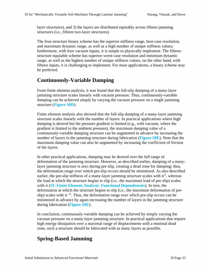
SI for “Mechanically Versatile Soft Machines Through Laminar Jamming” Narang, Vlassak, and Howe
Initial Submission to Advanced Functional Materials SI Page 33
layer structures), and 3) the layers are distributed equitably across fifteen jamming
structures (i.e., fifteen two-layer structures).
The four-structure binary scheme has the superior stiffness range, best-case resolution,
and maximum dynamic range, as well as a high number of unique stiffness values;
furthermore, with four vacuum inputs, it is simple to physically implement. The fifteen-
structure equitable scheme has superior worst-case resolution and minimum dynamic
range, as well as the highest number of unique stiffness values; on the other hand, with
fifteen inputs, it is challenging to implement. For most applications, a binary scheme may
be preferred.
Continuously-Variable Damping
From finite element analysis, it was found that the full-slip damping of a many-layer
jamming structure scales linearly with vacuum pressure. Thus, continuously-variable
damping can be achieved simply by varying the vacuum pressure on a single jamming
structure (Figure S8D).
Finite element analysis also showed that the full-slip damping of a many-layer jamming
structure scales linearly with the number of layers. In practical applications where high
damping is desired but the pressure gradient is limited (e.g., with vacuum, where the
gradient is limited to the ambient pressure), the maximum damping value of a
continuously-variable damping structure can be augmented in advance by increasing the
number of layers in the jamming structure during fabrication (Figure S8E). Note that the
maximum damping value can also be augmented by increasing the coefficient of friction
of the layers.
In other practical applications, damping may be desired over the full range of
deformation of the jamming structure. However, as described earlier, damping of a many-
layer jamming structure is zero during pre-slip, creating a dead zone for damping; thus,
the deformation range over which pre-slip occurs should be minimized. As also described
earlier, the pre-slip stiffness of a many-layer jamming structure scales with 𝑛3, whereas
the load at which the structure begins to slip (i.e., the maximum load of pre-slip) scales
with 𝑛 (SI: Finite Element Analysis: Functional Dependencies). In turn, the
deformation at which the structure begins to slip (i.e., the maximum deformation of pre-
slip) scales with 𝑛−2. Thus, the deformation range over which pre-slip occurs can be
minimized in advance by again increasing the number of layers in the jamming structure
during fabrication (Figure S8E).
In conclusion, continuously-variable damping can be achieved by simply varying the
vacuum pressure on a many-layer jamming structure. In practical applications that require
high energy dissipation over a maximal range of displacements with a minimal dead
zone, such a structure should be fabricated with as many layers as possible.
Spring-Based Jamming
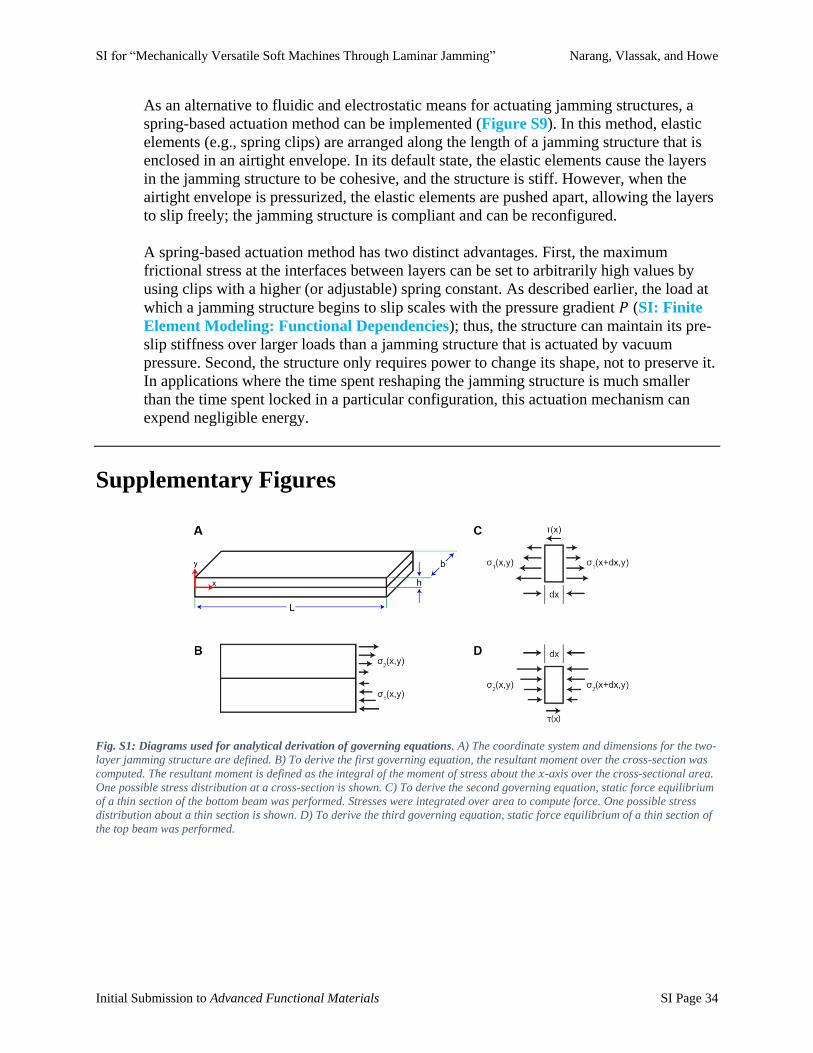
SI for “Mechanically Versatile Soft Machines Through Laminar Jamming” Narang, Vlassak, and Howe
Initial Submission to Advanced Functional Materials SI Page 34
As an alternative to fluidic and electrostatic means for actuating jamming structures, a
spring-based actuation method can be implemented (Figure S9). In this method, elastic
elements (e.g., spring clips) are arranged along the length of a jamming structure that is
enclosed in an airtight envelope. In its default state, the elastic elements cause the layers
in the jamming structure to be cohesive, and the structure is stiff. However, when the
airtight envelope is pressurized, the elastic elements are pushed apart, allowing the layers
to slip freely; the jamming structure is compliant and can be reconfigured.
A spring-based actuation method has two distinct advantages. First, the maximum
frictional stress at the interfaces between layers can be set to arbitrarily high values by
using clips with a higher (or adjustable) spring constant. As described earlier, the load at
which a jamming structure begins to slip scales with the pressure gradient 𝑃 (SI: Finite
Element Modeling: Functional Dependencies); thus, the structure can maintain its pre-
slip stiffness over larger loads than a jamming structure that is actuated by vacuum
pressure. Second, the structure only requires power to change its shape, not to preserve it.
In applications where the time spent reshaping the jamming structure is much smaller
than the time spent locked in a particular configuration, this actuation mechanism can
expend negligible energy.
Supplementary Figures
Fig. S1: Diagrams used for analytical derivation of governing equations. A) The coordinate system and dimensions for the two-
layer jamming structure are defined. B) To derive the first governing equation, the resultant moment over the cross-section was
computed. The resultant moment is defined as the integral of the moment of stress about the 𝑥-axis over the cross-sectional area.
One possible stress distribution at a cross-section is shown. C) To derive the second governing equation, static force equilibrium
of a thin section of the bottom beam was performed. Stresses were integrated over area to compute force. One possible stress
distribution about a thin section is shown. D) To derive the third governing equation, static force equilibrium of a thin section of
the top beam was performed.
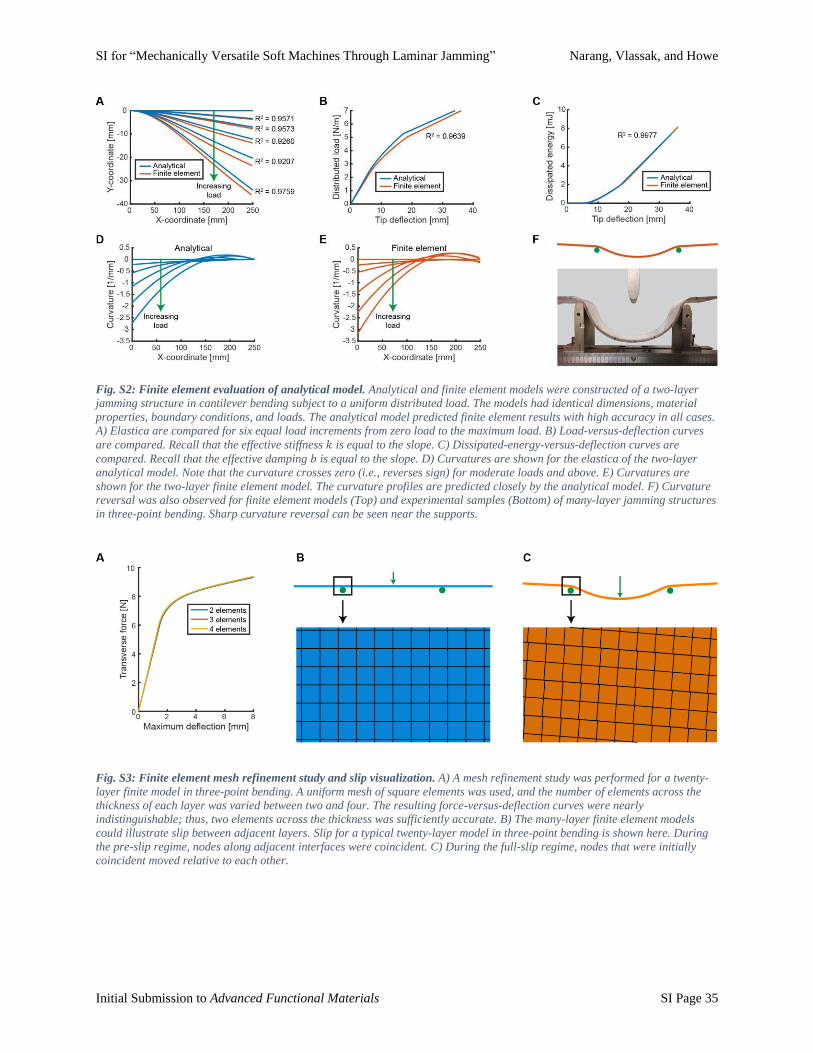
SI for “Mechanically Versatile Soft Machines Through Laminar Jamming” Narang, Vlassak, and Howe
Initial Submission to Advanced Functional Materials SI Page 35
Fig. S2: Finite element evaluation of analytical model. Analytical and finite element models were constructed of a two-layer
jamming structure in cantilever bending subject to a uniform distributed load. The models had identical dimensions, material
properties, boundary conditions, and loads. The analytical model predicted finite element results with high accuracy in all cases.
A) Elastica are compared for six equal load increments from zero load to the maximum load. B) Load-versus-deflection curves
are compared. Recall that the effective stiffness 𝑘 is equal to the slope. C) Dissipated-energy-versus-deflection curves are
compared. Recall that the effective damping 𝑏 is equal to the slope. D) Curvatures are shown for the elastica of the two-layer
analytical model. Note that the curvature crosses zero (i.e., reverses sign) for moderate loads and above. E) Curvatures are
shown for the two-layer finite element model. The curvature profiles are predicted closely by the analytical model. F) Curvature
reversal was also observed for finite element models (Top) and experimental samples (Bottom) of many-layer jamming structures
in three-point bending. Sharp curvature reversal can be seen near the supports.
Fig. S3: Finite element mesh refinement study and slip visualization. A) A mesh refinement study was performed for a twenty-
layer finite model in three-point bending. A uniform mesh of square elements was used, and the number of elements across the
thickness of each layer was varied between two and four. The resulting force-versus-deflection curves were nearly
indistinguishable; thus, two elements across the thickness was sufficiently accurate. B) The many-layer finite element models
could illustrate slip between adjacent layers. Slip for a typical twenty-layer model in three-point bending is shown here. During
the pre-slip regime, nodes along adjacent interfaces were coincident. C) During the full-slip regime, nodes that were initially
coincident moved relative to each other.

SI for “Mechanically Versatile Soft Machines Through Laminar Jamming” Narang, Vlassak, and Howe
Initial Submission to Advanced Functional Materials SI Page 36
Fig. S4: Fabrication process for real-world jamming structures. The fabrication process is illustrated for a typical sample of a
many-layer jamming structure. A) A sheet of copy paper was placed on the bed of a laser cutter, and strips were cut along the
machine direction. B) Acrylic was placed on the bed of the laser cutter, and a frame was cut. C) The frame was coated in PTFE
tape and positioned on the bed of a vacuum former. A thin sheet of TPU was formed to the frame. D) The frame and TPU sheet
were positioned on the bed of a heat press. The strips of paper and a segment of TPU tubing were placed inside, and the TPU
sheet was folded to cover the contents. E) Aluminum blocks with a circular channel were arranged on the top and bottom of the
end of the jamming structure, sandwiching the TPU tubing between the two sides of the TPU envelope. F) Fabrication of the
sample was completed.
Fig. S5: Testing setup and repeatability analysis for experimental characterization of jamming structures. A) The jamming
structure was placed in a test fixture for three-point bending, which consisted of a loading anvil and two roller supports. The
loading anvil was attached to a load cell, and the jamming structure was connected to a vacuum regulator via flexible tubing to
mitigate parasitic loading of the tubing on the sample. B-F) Testing results for five twenty-layer jamming structures are shown in
sequence. For each sample, a mean curve is plotted, along with a shaded error bar that spans ±1 standard deviation from the
mean. The maximum standard deviation at any deflection is given. The structures were highly repeatable from trial to trial. G)
The mean curves for all five samples were then aggregated. A mean curve of the mean curves is plotted, along with a shaded
error bar. The structures were highly repeatable from sample to sample.

SI for “Mechanically Versatile Soft Machines Through Laminar Jamming” Narang, Vlassak, and Howe
Initial Submission to Advanced Functional Materials SI Page 37
Fig. S6: Finite element predictions and experimental characterization of damping in many-layer jamming structures.
Jamming structures were loaded in three-point bending and subsequently unloaded. Transverse force is plotted against maximum
deflection; dashed lines indicate finite element predictions, and colored lines denote experimental results. Finite element models
accurately predicted experimentally observed hysteresis. The area under the hysteresis curves is equal to the energy dissipated
over the loading cycle, and the effective damping 𝑑 is equal to the energy dissipated per unit deflection. A) The number of layers
in the jamming structures was varied. B) Vacuum pressure was varied. No finite element data is provided for the 0 𝑘𝑃𝑎 case, as
the model was unstable. C) Coefficient of friction was varied. No experimental data is shown, as coefficients of friction could not
be precisely varied experimentally.
Fig. S7: Testing device for measuring the torsional stiffness of a variable kinematics system. A) Front view of the testing
device. A variable kinematics structure is hung vertically. Its upper end is bolted in place, and its lower end is coupled to a cable
that is connected to a force gauge. B) Zoom view of the lower end of the testing device. Two plastic pins are embedded in the
variable kinematics structure and fastened to a pulley, and the cable is wound around the pulley. When the cable is pulled, the
pulley spins around a bushing, and the variable kinematics structure is twisted about its longitudinal axis. C) Physical
implementation of the testing device. The variable kinematics structure was originally oriented as shown in A and B; its lower
end has now been twisted by approximately 80°.

SI for “Mechanically Versatile Soft Machines Through Laminar Jamming” Narang, Vlassak, and Howe
Initial Submission to Advanced Functional Materials SI Page 38
Fig. S8: Conceptual examples of continuously-variable stiffness and damping structures. For simplicity, transition regimes
between the pre-slip regime and the full-slip regime are not depicted. A) In one implementation of continuously-variable stiffness,
four jamming structures are stacked and bonded. Each jamming structure has an independent vacuum input and contains three
layers of compliant material. B) By applying or relieving vacuum from individual jamming structures, the pre-slip bending
stiffness of the composite structure may be selected from one of five possible values. C) For a continuously-variable stiffness
structure consisting of thirty total layers, three different ways are considered for distributing the layers across multiple jamming
structures. Quantity 𝑘 is the bending stiffness of a single layer. A four-structure binary scheme is preferable over equitable and
near-equitable schemes, as it has the best stiffness range, resolution, and dynamic range, and it is simple to physically
implement. D) Conceptual load-versus-deflection curves are shown for a continuously-variable damping structure. (Because it
may be desirable to use such a structure over multiple cycles, a full hysteresis loop is shown; the structure is loaded, unloaded,
and then loaded and unloaded in the opposite direction to return to zero deflection.) Increasing the vacuum pressure augments
the dissipated energy (i.e., the area enclosed by the hysteresis loop) and damping (i.e., the dissipated energy per unit deflection).
E) Increasing the number of layers again augments damping. Furthermore, it minimizes the range of deformation over which the
pre-slip regime occurs, maximizing the range over which damping is nonzero.
Fig. S9: Conceptual example of a spring-based jamming structure. A many-layer jamming structure enclosed in an airtight
envelope is connected to a compressed air source and has spring clips arranged along its length. When no air is supplied, the
spring clips cause the layers to be cohesive, and the structure is stiff. When air is supplied, the clips are pushed open, and the
layers can slip freely. The structure is then compliant and may be reconfigured.
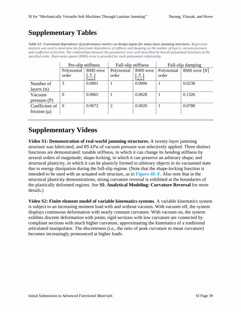
SI for “Mechanically Versatile Soft Machines Through Laminar Jamming” Narang, Vlassak, and Howe
Initial Submission to Advanced Functional Materials SI Page 39
Supplementary Tables Table S1: Functional dependence of performance metrics on design inputs for many-layer jamming structures. Regression
analysis was used to determine the functional dependence of stiffness and damping on the number of layers, vacuum pressure,
and coefficient of friction. The relationships between the parameters were well-described by best-fit polynomial functions of the
specified order. Root-mean-square (RMS) error is provided for each polynomial relationship.
Pre-slip stiffness Full-slip stiffness Full-slip damping
Polynomial
order
RMS error
[𝑁
𝑚𝑚]
Polynomial
order
RMS error
[𝑁
𝑚𝑚]
Polynomial
order
RMS error [𝑁]
Number of
layers (n)
3 0.0001 1 0.0006 1 0.0238
Vacuum
pressure (P)
0 0.0065 1 0.0028 1 0.1326
Coefficient of
friction (μ)
0 0.0072 2 0.0020 1 0.0788
Supplementary Videos
Video S1: Demonstration of real-world jamming structures. A twenty-layer jamming
structure was fabricated, and 85 𝑘𝑃𝑎 of vacuum pressure was selectively applied. Three distinct
functions are demonstrated: tunable stiffness, in which it can change its bending stiffness by
several orders of magnitude; shape-locking, in which it can preserve an arbitrary shape; and
structural plasticity, in which it can be plasticly formed to arbitrary objects in its vacuumed state
due to energy dissipation during the full-slip regime. (Note that the shape-locking function is
intended to be used with an actuated soft structure, as in Figure 4E-F. Also note that in the
structural plasticity demonstrations, strong curvature reversal is exhibited at the boundaries of
the plastically deformed regions. See SI: Analytical Modeling: Curvature Reversal for more
details.)
Video S2: Finite element model of variable kinematics systems. A variable kinematics system
is subject to an increasing moment load with and without vacuum. With vacuum off, the system
displays continuous deformation with nearly constant curvature. With vacuum on, the system
exhibits discrete deformation with joints; rigid sections with low curvature are connected by
compliant sections with much higher curvature, approximating the kinematics of a traditional
articulated manipulator. The discreteness (i.e., the ratio of peak curvature to mean curvature)
becomes increasingly pronounced at higher loads.