mechanics and strength of material - nashua school …s handbook 27th/27_mech_02a.pdf335 torsion...
TRANSCRIPT
TABLE OF CONTENTS
138
MECHANICS
141 Terms and Definitions142 Unit Systems142 Gravity142 Metric system (SI)145 Force Systems145 Scalar and Vector Quantities145 Graphical Resolution of Forces147 Couples and Forces148 Resolution of Force Systems149 Subtraction and Addition of Force153 Forces in Two or More Planes154 Parallel Forces155 Nonparallel Forces157 Friction157 Laws of Friction158 Coefficients of Friction158 Static Friction Coefficients159 Rolling Friction159 Mechanisms159 Levers161 Inclined Plane, Wedge162 Wheels and Pulleys163 Screw163 Geneva Wheel164 Toggle Joint165 Pendulums166 Harmonic
VELOCITY, ACCELERATION, WORK, AND ENERGY
167 Velocity and Acceleration167 Newton's Laws of Motion167 Constant Velocity167 Constant Acceleration168 Angular Velocity169 Linear Velocity of Rotating Body169 Rotary Motion with Acceleration171 Force, Work, Energy, Momentum171 Acceleration by Forces172 Torque and Angular Acceleration173 Energy174 Work Performed by Forces174 Work and Energy175 Force of a Blow176 Impulse and Momentum178 Work and Power179 Centrifugal Force180 Centrifugal Casting
FLYWHEELS
183 Classification184 Energy by Velocity184 Flywheel Design185 Flywheels for Presses, Punches
and Shears186 Dimensions of Flywheels187 Simplified Flywheel Calculations188 Centrifugal Stresses in Flywheels189 Combined Stresses in Flywheels189 Thickness of Flywheel Rims190 Safety Factors190 Safe Rim Speeds191 Safe Rotation Speeds192 Bursting Speeds193 Stresses in Rotating Disks193 Steam Engine Flywheels194 Spokes or Arms of Flywheels195 Critical Speeds196 Critical Speed Formulas197 Balancing Rotating Parts197 Static and Dynamic Balancing197 Balancing Calculations198 Masses in Same Plane200 Masses in Two or More Planes201 Balancing Lathe Fixtures
STRENGTH OF MATERIALS
203 Properties of Materials204 Yield Point, Elastic Modulus and
Poission’s Ratio205 Compressive, Shear Properties205 Creep207 Fatigue Failure208 Stress208 Factors of Safety208 Working Stress209 Stress Concentration Factors213 Simple Stresses214 Deflections215 Combined Stresses215 Tables of Combined Stresses219 Three-dimensional Stress221 Sample Calculations223 Stresses in a Loaded Ring224 Strength of Taper Pins
MECHANICS AND STRENGTH OF MATERIALS
Machinery's Handbook 27th Edition
Copyright 2004, Industrial Press, Inc., New York, NY
TABLE OF CONTENTS
139
MECHANICS AND STRENGTH OF MATERIALS
PROPERTIES OF BODIES
225 Center of Gravity232 Radius of Gyration235 Center and Radius of Oscillation 235 Center of Percussion236 Moment of Inertia237 Calculating For Built-up Sections 238 Area Moments of Inertia, Section
Moduli and Radius of Gyration248 Polar Area Moment of Inertia and
Section Modulus248 Mass Moment of Inertia250 Polar Mass Moments of Inertia253 Tables for Rectangles and Shafts
BEAMS
260 Beam Calculations261 Stress and Deflection Beam Table272 Rectangular Solid Beams273 Round Solid Beams277 Deflection as Limiting Factor278 Curved Beams281 Size of Rail to Carry Load281 American Railway Engineering
Association Formulas282 Stresses Produced by Shocks282 Beam Stresses Due to Shock283 Stresses in Helical Springs284 Fatigue Stresses
COLUMNS
285 Strength of Columns or Struts285 Rankine or Gordon Formula285 Straight-line Formula285 Formulas of American Railway
Engineering Association286 Euler Formula286 Eccentrically Loaded Columns289 AISC Formulas
PLATES, SHELLS, AND CYLINDERS
292 Square Flat Plates294 Circular Flat Plates294 Cylinders, Internal Pressure295 Spherical Shells, Internal Pressure297 Cylinders, External Pressure
SHAFTS
299 Shaft Calculations299 Torsional Strength of Shafting301 Torsional Deflections302 Linear Deflections303 Design of Transmission Shafting305 Effect of Keyways305 Brittle Materials306 Critical Speeds 306 Shaft Couplings307 Hollow and Solid Shafts
SPRINGS
308 Introduction to Spring Design308 Notation309 Spring Materials309 High-Carbon Spring Steels310 Alloy Spring Steels310 Stainless Spring Steels311 Copper-Base Spring Alloys312 Nickel-Base Spring Alloys313 Spring Stresses313 Working Stresses 318 Endurance Limit 319 Working Stresses at Elevated
Temperatures320 Spring Design Data320 Spring Characteristics320 Compression Spring Design321 Formulas for Compression Spring324 Spring Characteristics329 Extension Springs331 Bending Stress331 Extension Spring Design333 Tolerances for Compression and
Extension Springs335 Torsion Spring Design342 Torsion Spring Characteristics347 Torsion Spring Tolerances348 Miscellaneous Springs348 Flat Springs Formula349 Moduli of Elasticity349 Heat Treatment of Springs352 Spring Failure352 Causes of Spring Failure353 Music Wire
Machinery's Handbook 27th Edition
Copyright 2004, Industrial Press, Inc., New York, NY
TABLE OF CONTENTS
140
MECHANICS AND STRENGTH OF MATERIALS
DISC SPRINGS
354 Performance of Disc Springs354 Introduction354 Nomenclature354 Group Classifications355 Contact Surfaces355 Materials356 Stacking of Disc Springs358 Disc Spring Forces and Stresses358 Springs Without Contact Surfaces361 Springs Without Contact Surfaces361 Functional Stresses362 Fatigue Life365 Recommended Dimensional
Ratios365 Example Applications
WIRE ROPE, CHAIN,ROPE, AND HOOKS
369 Strength and Properties of Wire Rope
369 Wire Rope Construction370 Properties of Wire Rope371 Classes of Wire Rope372 Weights and Strengths376 Sizes and Strengths377 Factors of Safety378 Installing Wire Rope379 Drum and Reel Capacities380 Pressures for Drums and Sheaves380 Sheave and Drum Groove
Dimensions381 Cutting and Seizing381 Maintenance381 Lubrication of Wire Rope
WIRE ROPE, CHAIN,
(Continued)ROPE, AND HOOKS
382 Wire Rope Slings and Fittings382 Slings382 Wire Rope Fittings382 Applying Clips and Attaching
Sockets384 Capacities of Wire Rope and
Slings386 Crane Chain and Hooks386 Material for Crane Chains386 Strength of Chains386 Hoisting and Crane Chains386 Maximum Wear on a Link387 Safe Loads for Ropes and Chains388 Strength of Manila Rope390 Loads Lifted by Crane Chains391 Winding Drum Scores for Chain391 Sprocket Wheels for Link Chains 393 Crane Hooks393 Making an Eye-splice394 Eye-bolts395 Eye Nuts and Lift Eyes
Machinery's Handbook 27th Edition
Copyright 2004, Industrial Press, Inc., New York, NY
MECHANICS AND STRENGTH OF MATERIALS 141
MECHANICS
Throughout this section in this Handbook, both English and metric SI data and for-mulas are given to cover the requirements of working in either system of measure-ment. Except for the passage entitled The Use of the Metric SI System in MechanicsCalculations, formulas and text relating exclusively to SI are given in bold face type.
Terms and Definitions
Definitions.—The science of mechanics deals with the effects of forces in causing or pre-venting motion. Statics is the branch of mechanics that deals with bodies in equilibrium,i.e., the forces acting on them cause them to remain at rest or to move with uniform veloc-ity. Dynamics is the branch of mechanics that deals with bodies not in equilibrium, i.e., theforces acting on them cause them to move with non-uniform velocity. Kinetics is thebranch of dynamics that deals with both the forces acting on bodies and the motions thatthey cause. Kinematics is the branch of dynamics that deals only with the motions of bodieswithout reference to the forces that cause them.
Definitions of certain terms and quantities as used in mechanics follow: Force may be defined simply as a push or a pull; the push or pull may result from the
force of contact between bodies or from a force, such as magnetism or gravitation, in whichno direct contact takes place.
Matter is any substance that occupies space; gases, liquids, solids, electrons, atoms,molecules, etc., all fit this definition.
Inertia is the property of matter that causes it to resist any change in its motion or state ofrest.
Mass is a measure of the inertia of a body. Work, in mechanics, is the product of force times distance and is expressed by a combi-
nation of units of force and distance, as foot-pounds, inch-pounds, meter-kilograms, etc.The metric SI unit of work is the joule, which is the work done when the point of appli-cation of a force of one newton is displaced through a distance of one meter in thedirection of the force.
Power, in mechanics, is the product of force times distance divided by time; it measuresthe performance of a given amount of work in a given time. It is the rate of doing work andas such is expressed in foot-pounds per minute, foot-pounds per second, kilogram-metersper second, etc. The metric SI unit is the watt, which is one joule per second.
Horsepower is the unit of power that has been adopted for engineering work. One horse-power is equal to 33,000 foot-pounds per minute or 550 foot-pounds per second. The kilo-watt, used in electrical work, equals 1.34 horsepower; or 1 horsepower equals 0.746kilowatt. However, in the metric SI, the term horsepower is not used, and the basicunit of power is the watt. This unit, and the derived units milliwatt and kilowatt, forexample, are the same as those used in electrical work.
Torque or moment of a force is a measure of the tendency of the force to rotate the bodyupon which it acts about an axis. The magnitude of the moment due to a force acting in aplane perpendicular to some axis is obtained by multiplying the force by the perpendiculardistance from the axis to the line of action of the force. (If the axis of rotation is not perpen-dicular to the plane of the force, then the components of the force in a plane perpendicularto the axis of rotation are used to find the resultant moment of the force by finding themoment of each component and adding these component moments algebraically.)Moment or torque is commonly expressed in pound-feet, pound-inches, kilogram-meters,etc. The metric SI unit is the newton-meter (N · m).
Velocity is the time-rate of change of distance and is expressed as distance divided bytime, that is, feet per second, miles per hour, centimeters per second, meters per second,etc.
Machinery's Handbook 27th Edition
Copyright 2004, Industrial Press, Inc., New York, NY

142 MECHANICS
Acceleration is defined as the time-rate of change of velocity and is expressed as veloc-ity divided by time or as distance divided by time squared, that is, in feet per second, persecond or feet per second squared; inches per second, per second or inches per secondsquared; centimeters per second, per second or centimeters per second squared; etc. Themetric SI unit is the meter per second squared.Unit Systems.—In mechanics calculations, both absolute and gravitational systems ofunits are employed. The fundamental units in absolute systems are length, time, and mass,and from these units, the dimension of force is derived. Two absolute systems which havebeen in use for many years are the cgs (centimeter-gram-second) and the MKS (meter-kilogram-second) systems. Another system, known as MKSA (meter-kilogram-second-ampere), links the MKS system of units of mechanics with electro magnetic units.
The Conference General des Poids et Mesures (CGPM), which is the body responsi-ble for all international matters concerning the metric system, adopted in 1954 arationalized and coherent system of units based on the four MKSA units and includ-ing the kelvin as the unit of temperature, and the candela as the unit of luminousintensity. In 1960, the CGPM formally named this system the ‘Systeme Internationald'Unites,’ for which the abbreviation is SI in all languages. In 1971, the 14th CGPMadopted a seventh base unit, the mole, which is the unit of quantity (“amount of sub-stance”). Further details of the SI are given in the section MEASURING UNITS start-ing on page 2544, and its application in mechanics calculations, contrasted with theuse of the English system, is considered on page 142.
The fundamental units in gravitational systems are length, time, and force, and fromthese units, the dimension of mass is derived. In the gravitational system most widely usedin English measure countries, the units of length, time, and force are, respectively, the foot,the second, and the pound. The corresponding unit of mass, commonly called the slug, isequal to 1 pound second2 per foot and is derived from the formula, M = W ÷ g in which M =mass in slugs, W = weight in pounds, and g = acceleration due to gravity, commonly takenas 32.16 feet per second2. A body that weighs 32.16 lbs. on the surface of the earth has,therefore, a mass of one slug.
Many engineering calculations utilize a system of units consisting of the inch, the sec-ond, and the pound. The corresponding units of mass are pounds second2 per inch and thevalue of g is taken as 386 inches per second2.
In a gravitational system that has been widely used in metric countries, the units oflength, time, and force are, respectively, the meter, the second, and the kilogram. The cor-responding units of mass are kilograms second2 per meter and the value of g is taken as9.81 meters per second2.Acceleration of Gravity g Used in Mechanics Formulas.—The acceleration of a freelyfalling body has been found to vary according to location on the earth’s surface as well aswith height, the value at the equator being 32.09 feet per second, per second while at thepoles it is 32.26 ft/sec2. In the United States it is customary to regard 32.16 as satisfactoryfor most practical purposes in engineering calculations.
Standard Pound Force: For use in defining the magnitude of a standard unit of force,known as the pound force, a fixed value of 32.1740 ft/sec2, designated by the symbol g0,has been adopted by international agreement. As a result of this agreement, whenever theterm mass, M, appears in a mechanics formula and the substitution M = W/g is made, use ofthe standard value g0 = 32.1740 ft/sec2 is implied although as stated previously, it is cus-tomary to use approximate values for g except where extreme accuracy is required.The Use of the Metric SI System in Mechanics Calculations.—The SI system is adevelopment of the traditional metric system based on decimal arithmetic; fractions areavoided. For each physical quantity, units of different sizes are formed by multiplying ordividing a single base value by powers of 10. Thus, changes can be made very simply by
Machinery's Handbook 27th Edition
Copyright 2004, Industrial Press, Inc., New York, NY
MECHANICS 143
adding zeros or shifting decimal points. For example, the meter is the basic unit of length;the kilometer is a multiple (1,000 meters); and the millimeter is a sub-multiple (one-thou-sandth of a meter).
In the older metric system, the simplicity of a series of units linked by powers of 10 is anadvantage for plain quantities such as length, but this simplicity is lost as soon as morecomplex units are encountered. For example, in different branches of science and engi-neering, energy may appear as the erg, the calorie, the kilogram-meter, the liter-atmo-sphere, or the horsepower-hour. In contrast, the SI provides only one basic unit for eachphysical quantity, and universality is thus achieved.
There are seven base-units, and in mechanics calculations three are used, which are forthe basic quantities of length, mass, and time, expressed as the meter (m), the kilogram(kg), and the second (s). The other four base-units are the ampere (A) for electric current,the kelvin (K) for thermodynamic temperature, the candela (cd) for luminous intensity,and the mole (mol) for amount of substance.
The SI is a coherent system. A system of units is said to be coherent if the product or quo-tient of any two unit quantities in the system is the unit of the resultant quantity. For exam-ple, in a coherent system in which the foot is a unit of length, the square foot is the unit ofarea, whereas the acre is not. Further details of the SI, and definitions of the units, are givenin the section MEASURING UNITS starting on page 2544, near the end of the book.
Other physical quantities are derived from the base-units. For example, the unit of veloc-ity is the meter per second (m/s), which is a combination of the base-units of length andtime. The unit of acceleration is the meter per second squared (m/s2). By applying New-ton's second law of motion — force is proportional to mass multiplied by acceleration —the unit of force is obtained, which is the kg · m/s2. This unit is known as the newton, or N.Work, or force times distance, is the kg · m2/s2, which is the joule, (1 joule = 1 newton-meter) and energy is also expressed in these terms. The abbreviation for joule is J. Power,or work per unit time, is the kg · m2/s3, which is the watt (1 watt = 1 joule per second = 1newton-meter per second). The abbreviation for watt is W.
More information on Newton’s laws may be found in the section Newton' s Laws ofMotion on page 167.
The coherence of SI units has two important advantages. The first, that of uniqueness andtherefore universality, has been explained. The second is that it greatly simplifies technicalcalculations. Equations representing physical principles can be applied without introduc-ing such numbers as 550 in power calculations, which, in the English system of measure-ment have to be used to convert units. Thus conversion factors largely disappear fromcalculations carried out in SI units, with a great saving in time and labor.
Mass, Weight, Force, Load: SI is an absolute system (see Unit Systems on page 142), andconsequently it is necessary to make a clear distinction between mass and weight. Themass of a body is a measure of its inertia, whereas the weight of a body is the force exertedon it by gravity. In a fixed gravitational field, weight is directly proportional to mass, andthe distinction between the two can be easily overlooked. However, if a body is moved to adifferent gravitational field, for example, that of the moon, its weight alters, but its massremains unchanged. Since the gravitational field on earth varies from place to place byonly a small amount, and weight is proportional to mass, it is practical to use the weight ofunit mass as a unit of force, and this procedure is adopted in both the English and older met-ric systems of measurement. In common usage, they are given the same names, and we saythat a mass of 1 pound has a weight of 1 pound. In the former case the pound is being usedas a unit of mass, and in the latter case, as a unit of force. This procedure is convenient insome branches of engineering, but leads to confusion in others.
As mentioned earlier, Newton's second law of motion states that force is proportional tomass times acceleration. Because an unsupported body on the earth's surface falls withacceleration g (32 ft/s2 approximately), the pound (force) is that force which will impart an
Machinery's Handbook 27th Edition
Copyright 2004, Industrial Press, Inc., New York, NY
144 MECHANICS
acceleration of g ft/s2 to a pound (mass). Similarly, the kilogram (force) is that force whichwill impart an acceleration of g (9.8 meters per second2 approximately), to a mass of onekilogram. In the SI, the newton is that force which will impart unit acceleration (1 m/s2) toa mass of one kilogram. It is therefore smaller than the kilogram (force) in the ratio 1:g(about 1:9.8). This fact has important consequences in engineering calculations. The factorg now disappears from a wide range of formulas in dynamics, but appears in many formu-las in statics where it was formerly absent. It is however not quite the same g, for reasonswhich will now be explained.
In the article on page 171, the mass of a body is referred to as M, but it is immediatelyreplaced in subsequent formulas by W/g, where W is the weight in pounds (force), whichleads to familiar expressions such as WV2 / 2g for kinetic energy. In this treatment, the Mwhich appears briefly is really expressed in terms of the slug (page 142), a unit normallyused only in aeronautical engineering. In everyday engineers’ language, weight and massare regarded as synonymous and expressions such as WV2 / 2g are used without ponderingthe distinction. Nevertheless, on reflection it seems odd that g should appear in a formulawhich has nothing to do with gravity at all. In fact the g used here is not the true, local valueof the acceleration due to gravity, but an arbitrary standard value which has been chosen aspart of the definition of the pound (force) and is more properly designated go (page 142).Its function is not to indicate the strength of the local gravitational field, but to convert fromone unit to another.
In the SI the unit of mass is the kilogram, and the unit of force (and therefore weight) isthe newton.
The following are typical statements in dynamics expressed in SI units:A force of R newtons acting on a mass of M kilograms produces an acceleration of R/M
meters per second2. The kinetic energy of a mass of M kg moving with velocity V m/s is 1⁄2MV2 kg (m/s)2 or 1⁄2 MV2 joules. The work done by a force of R newtons moving a distanceL meters is RL Nm, or RL joules. If this work were converted entirely into kinetic energywe could write RL = 1⁄2 MV2 and it is instructive to consider the units. Remembering that theN is the same as the kg · m/s2, we have (kg · m/s)2 × m = kg (m/s)2, which is obviously cor-rect. It will be noted that g does not appear anywhere in these statements.
In contrast, in many branches of engineering where the weight of a body is important,rather than its mass, using SI units, g does appear where formerly it was absent. Thus, if arope hangs vertically supporting a mass of M kilograms the tension in the rope is Mg N.Here g is the acceleration due to gravity, and its units are m/s2. The ordinary numericalvalue of 9.81 will be sufficiently accurate for most purposes on earth. The expression isstill valid elsewhere, for example, on the moon, provided the proper value of g is used. Themaximum tension the rope can safely withstand (and other similar properties) will also bespecified in terms of the newton, so that direct comparison may be made with the tensionpredicted.
Words like load and weight have to be used with greater care. In everyday language wemight say “a lift carries a load of five people of average weight 70 kg,” but in precise tech-nical language we say that if the average mass is 70 kg, then the average weight is 70g N,and the total load (that is force) on the lift is 350g N.
If the lift starts to rise with acceleration a · m/s2, the load becomes 350 (g + a) N; both gand a have units of m/s2, the mass is in kg, so the load is in terms of kg · m/s2, which is thesame as the newton.
Pressure and stress: These quantities are expressed in terms of force per unit area. In theSI the unit is the pascal (Pa), which expressed in terms of SI derived and base units is thenewton per meter squared (N/m2). The pascal is very small—it is only equivalent to 0.15 ×10⁻³ lb/in2 — hence the kilopascal (kPa = 1000 pascals), and the megapascal (MPa = 106
Machinery's Handbook 27th Edition
Copyright 2004, Industrial Press, Inc., New York, NY
FORCE SYSTEMS 145
pascals) may be more convenient multiples in practice. Thus, note: 1 newton per millime-ter squared = 1 meganewton per meter squared = 1 megapascal.
In addition to the pascal, the bar, a non-SI unit, is in use in the field of pressure measure-ment in some countries, including England. Thus, in view of existing practice, the Interna-tional Committee of Weights and Measures (CIPM) decided in 1969 to retain this unit fora limited time for use with those of SI. The bar = 105 pascals and the hectobar = 107 pascals.
Force Systems
Scalar and Vector Quantities.—The quantities dealt with in mechanics are of two kindsaccording to whether magnitude alone or direction as well as magnitude must be known inorder to completely specify them. Quantities such as time, volume and density are com-pletely specified when their magnitude is known. Such quantities are called scalar quanti-ties. Quantities such as force, velocity, acceleration, moment, and displacement whichmust, in order to be specified completely, have a specific direction as well as magnitude,are called vector quantities.
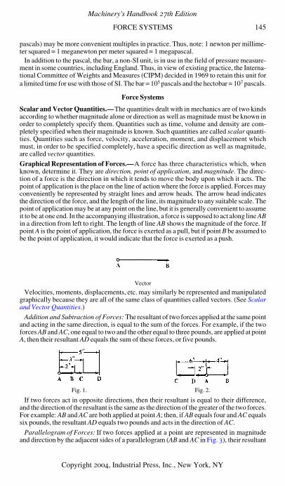
Graphical Representation of Forces.—A force has three characteristics which, whenknown, determine it. They are direction, point of application, and magnitude. The direc-tion of a force is the direction in which it tends to move the body upon which it acts. Thepoint of application is the place on the line of action where the force is applied. Forces mayconveniently be represented by straight lines and arrow heads. The arrow head indicatesthe direction of the force, and the length of the line, its magnitude to any suitable scale. Thepoint of application may be at any point on the line, but it is generally convenient to assumeit to be at one end. In the accompanying illustration, a force is supposed to act along line ABin a direction from left to right. The length of line AB shows the magnitude of the force. Ifpoint A is the point of application, the force is exerted as a pull, but if point B be assumed tobe the point of application, it would indicate that the force is exerted as a push.
Vector
Velocities, moments, displacements, etc. may similarly be represented and manipulatedgraphically because they are all of the same class of quantities called vectors. (See Scalarand Vector Quantities.)
Addition and Subtraction of Forces: The resultant of two forces applied at the same pointand acting in the same direction, is equal to the sum of the forces. For example, if the twoforces AB and AC, one equal to two and the other equal to three pounds, are applied at pointA, then their resultant AD equals the sum of these forces, or five pounds.
If two forces act in opposite directions, then their resultant is equal to their difference,and the direction of the resultant is the same as the direction of the greater of the two forces.For example: AB and AC are both applied at point A; then, if AB equals four and AC equalssix pounds, the resultant AD equals two pounds and acts in the direction of AC.
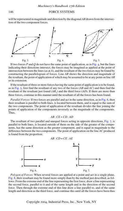
Parallelogram of Forces: If two forces applied at a point are represented in magnitudeand direction by the adjacent sides of a parallelogram (AB and AC in Fig. 3), their resultant
Fig. 1. Fig. 2.
Machinery's Handbook 27th Edition
Copyright 2004, Industrial Press, Inc., New York, NY
146 FORCE SYSTEMS
will be represented in magnitude and direction by the diagonal AR drawn from the intersec-tion of the two component forces.
If two forces P and Q do not have the same point of application, as in Fig. 4, but the linesindicating their directions intersect, the forces may be imagined as applied at the point ofintersection between the lines (as at A), and the resultant of the two forces may be found byconstructing the parallelogram of forces. Line AR shows the direction and magnitude ofthe resultant, the point of application of which may be assumed to be at any point on line ARor its extension.
If the resultant of three or more forces having the same point of application is to be found,as in Fig. 5, first find the resultant of any two of the forces (AB and AC) and then find theresultant of the resultant just found (AR1) and the third force (AD). If there are more thanthree forces, continue in this manner until the resultant of all the forces has been found.
Parallel Forces: If two forces are parallel and act in the same direction, as in Fig. 6, thentheir resultant is parallel to both lines, is located between them, and is equal to the sum ofthe two components. The point of application of the resultant divides the line joining thepoints of application of the components inversely as the magnitude of the components.Thus,
AB : CE = CD : AD
The resultant of two parallel and unequal forces acting in opposite directions, Fig. 7, isparallel to both lines, is located outside of them on the side of the greater of the compo-nents, has the same direction as the greater component, and is equal in magnitude to thedifference between the two components. The point of application on the line AC producedis found from the proportion:
AB : CD = CE : AE
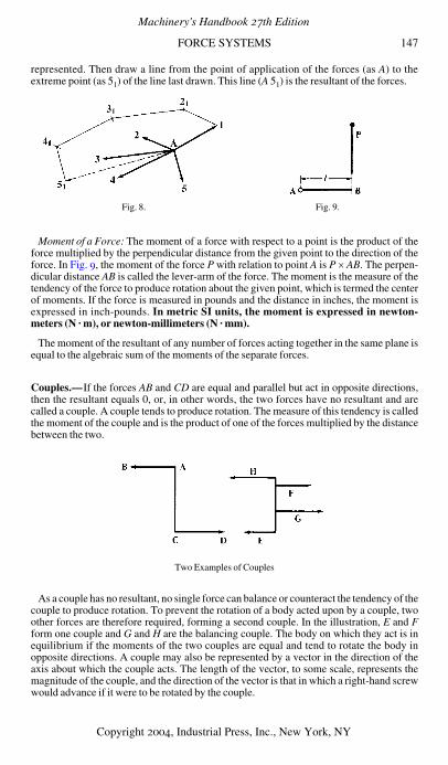
Polygon of Forces: When several forces are applied at a point and act in a single plane,Fig. 8, their resultant may be found more simply than by the method just described, as fol-lows: From the extreme end of the line representing the first force, draw a line representingthe second force, parallel to it and of the same length and in the direction of the secondforce. Then through the extreme end of this line draw a line parallel to, and of the samelength and direction as the third force, and continue this until all the forces have been thus
Fig. 3. Fig. 4. Fig. 5.
Fig. 6. Fig. 7.
Machinery's Handbook 27th Edition
Copyright 2004, Industrial Press, Inc., New York, NY
FORCE SYSTEMS 147
represented. Then draw a line from the point of application of the forces (as A) to theextreme point (as 51) of the line last drawn. This line (A 51) is the resultant of the forces.
Moment of a Force: The moment of a force with respect to a point is the product of theforce multiplied by the perpendicular distance from the given point to the direction of theforce. In Fig. 9, the moment of the force P with relation to point A is P × AB. The perpen-dicular distance AB is called the lever-arm of the force. The moment is the measure of thetendency of the force to produce rotation about the given point, which is termed the centerof moments. If the force is measured in pounds and the distance in inches, the moment isexpressed in inch-pounds. In metric SI units, the moment is expressed in newton-meters (N · m), or newton-millimeters (N · mm).
The moment of the resultant of any number of forces acting together in the same plane isequal to the algebraic sum of the moments of the separate forces.
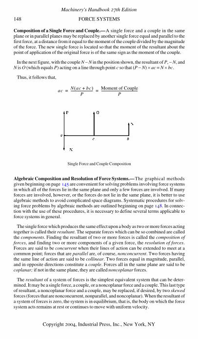
Couples.—If the forces AB and CD are equal and parallel but act in opposite directions,then the resultant equals 0, or, in other words, the two forces have no resultant and arecalled a couple. A couple tends to produce rotation. The measure of this tendency is calledthe moment of the couple and is the product of one of the forces multiplied by the distancebetween the two.
Two Examples of Couples
As a couple has no resultant, no single force can balance or counteract the tendency of thecouple to produce rotation. To prevent the rotation of a body acted upon by a couple, twoother forces are therefore required, forming a second couple. In the illustration, E and Fform one couple and G and H are the balancing couple. The body on which they act is inequilibrium if the moments of the two couples are equal and tend to rotate the body inopposite directions. A couple may also be represented by a vector in the direction of theaxis about which the couple acts. The length of the vector, to some scale, represents themagnitude of the couple, and the direction of the vector is that in which a right-hand screwwould advance if it were to be rotated by the couple.
Fig. 8. Fig. 9.
Machinery's Handbook 27th Edition
Copyright 2004, Industrial Press, Inc., New York, NY
148 FORCE SYSTEMS
Composition of a Single Force and Couple.—A single force and a couple in the sameplane or in parallel planes may be replaced by another single force equal and parallel to thefirst force, at a distance from it equal to the moment of the couple divided by the magnitudeof the force. The new single force is located so that the moment of the resultant about thepoint of application of the original force is of the same sign as the moment of the couple.
In the next figure, with the couple N − N in the position shown, the resultant of P, − N, andN is O (which equals P) acting on a line through point c so that (P − N) × ac = N × bc.
Thus, it follows that,
Single Force and Couple Composition
Algebraic Composition and Resolution of Force Systems.—The graphical methodsgiven beginning on page 145 are convenient for solving problems involving force systemsin which all of the forces lie in the same plane and only a few forces are involved. If manyforces are involved, however, or the forces do not lie in the same plane, it is better to usealgebraic methods to avoid complicated space diagrams. Systematic procedures for solv-ing force problems by algebraic methods are outlined beginning on page 148. In connec-tion with the use of these procedures, it is necessary to define several terms applicable toforce systems in general.
The single force which produces the same effect upon a body as two or more forces actingtogether is called their resultant. The separate forces which can be so combined are calledthe components. Finding the resultant of two or more forces is called the composition offorces, and finding two or more components of a given force, the resolution of forces.Forces are said to be concurrent when their lines of action can be extended to meet at acommon point; forces that are parallel are, of course, nonconcurrent. Two forces havingthe same line of action are said to be collinear. Two forces equal in magnitude, parallel,and in opposite directions constitute a couple. Forces all in the same plane are said to becoplanar; if not in the same plane, they are called noncoplanar forces.
The resultant of a system of forces is the simplest equivalent system that can be deter-mined. It may be a single force, a couple, or a noncoplanar force and a couple. This last typeof resultant, a noncoplanar force and a couple, may be replaced, if desired, by two skewedforces (forces that are nonconcurrent, nonparallel, and noncoplanar). When the resultant ofa system of forces is zero, the system is in equilibrium, that is, the body on which the forcesystem acts remains at rest or continues to move with uniform velocity.
ac N ac bc+( )
P--------------------------- Moment of Couple
P---------------------------------------------= =
Machinery's Handbook 27th Edition
Copyright 2004, Industrial Press, Inc., New York, NY
FORCE SYSTEMS 149
Algebraic Solution of Force Systems—All Forces in the Same Plane
Finding Two Concurrent Components of a Single Force:
Finding the Resultant of Two Concurrent Forces:
Finding the Resultant of Three or More Concurrent Forces:
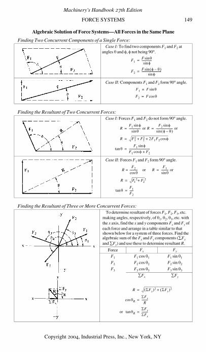
Case I: To find two components F1 and F2 at angles θ and φ, φ not being 90°.
Case II: Components F1 and F2 form 90° angle.
Case I: Forces F1 and F2 do not form 90° angle.
Case II: Forces F1 and F2 form 90° angle.
To determine resultant of forces F1, F2, F3, etc. making angles, respectively, of θ1, θ2, θ3, etc. with the x axis, find the x and y components Fx and Fy of each force and arrange in a table similar to that shown below for a system of three forces. Find the algebraic sum of the Fx and Fy components (∑Fx and ∑Fy) and use these to determine resultant R.
Force Fx Fy
F1 F1 cos θ1 F1 sin θ1
F2 F2 cos θ2 F2 sin θ2
F3 F3 cos θ3 F3 sin θ3
∑Fx ∑Fy
F1F θsin
φsin---------------=
F2F φ θ–( )sin
φsin-----------------------------=
F1 F θsin=
F2 F θcos=
RF1 φsin
θsin----------------- or R
F2 φsin
φ θ–( )sin------------------------- or= =
R F12 F2
2 2F1F2 φcos+ +=
θtanF1 φsin
F1 φcos F2+-------------------------------=
RF2
θcos------------= or R
F1
θsin----------- or=
R F12 F2
2+=
θtanF1
F2------=
R ΣFx( )2 ΣFy( )2+=
θRcosΣFx
R---------=
or θRtanΣFy
ΣFx---------=
Machinery's Handbook 27th Edition
Copyright 2004, Industrial Press, Inc., New York, NY
150 FORCE SYSTEMS
Finding a Force and a Couple Which Together are Equivalent to a Single Force:
Finding the Resultant of a Single Force and a Couple:
Finding the Resultant of a System of Parallel Forces:
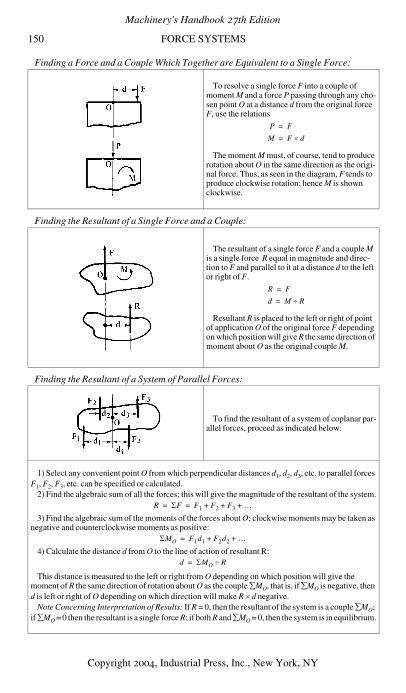
To resolve a single force F into a couple of moment M and a force P passing through any cho-sen point O at a distance d from the original force F, use the relations
The moment M must, of course, tend to produce rotation about O in the same direction as the origi-nal force. Thus, as seen in the diagram, F tends to produce clockwise rotation; hence M is shown clockwise.
The resultant of a single force F and a couple M is a single force R equal in magnitude and direc-tion to F and parallel to it at a distance d to the left or right of F.
Resultant R is placed to the left or right of point of application O of the original force F depending on which position will give R the same direction of moment about O as the original couple M.
To find the resultant of a system of coplanar par-allel forces, proceed as indicated below.
1) Select any convenient point O from which perpendicular distances d1, d2, d3, etc. to parallel forces F1, F2, F3, etc. can be specified or calculated.
2) Find the algebraic sum of all the forces; this will give the magnitude of the resultant of the system.
3) Find the algebraic sum of the moments of the forces about O; clockwise moments may be taken as negative and counterclockwise moments as positive:
4) Calculate the distance d from O to the line of action of resultant R:
This distance is measured to the left or right from O depending on which position will give the moment of R the same direction of rotation about O as the couple ∑MO, that is, if ∑MO is negative, then d is left or right of O depending on which direction will make R × d negative.
Note Concerning Interpretation of Results: If R = 0, then the resultant of the system is a couple ∑MO; if ∑MO = 0 then the resultant is a single force R; if both R and ∑MO = 0, then the system is in equilibrium.
P F=
M F d×=
R F=
d M R÷=
R ΣF F1 F2 F3 …+ + += =
ΣMO F1d1 F2d2 …+ +=
d ΣMO R÷=
Machinery's Handbook 27th Edition
Copyright 2004, Industrial Press, Inc., New York, NY
FORCE SYSTEMS 151
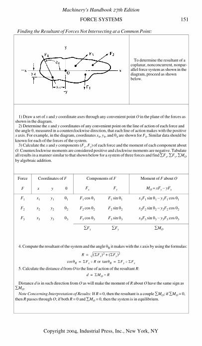
Finding the Resultant of Forces Not Intersecting at a Common Point:
To determine the resultant of a coplanar, nonconcurrent, nonpar-allel force system as shown in the diagram, proceed as shown below.
1) Draw a set of x and y coordinate axes through any convenient point O in the plane of the forces as shown in the diagram.
2) Determine the x and y coordinates of any convenient point on the line of action of each force and the angle θ, measured in a counterclockwise direction, that each line of action makes with the positive x axis. For example, in the diagram, coordinates x4, y4, and θ4 are shown for F4. Similar data should be known for each of the forces of the system.
3) Calculate the x and y components (Fx, Fy) of each force and the moment of each component about O. Counterclockwise moments are considered positive and clockwise moments are negative. Tabulate all results in a manner similar to that shown below for a system of three forces and find ∑Fx, ∑Fy, ∑MO by algebraic addition.
Force Coordinates of F Components of F Moment of F about O
F x y θ Fx Fy MO = xFy − yFx
F1 x1 y1 θ1 F1 cos θ1 F1 sin θ1 x1F1 sin θ1 − y1F1 cos θ1
F2 x2 y2 θ2 F2 cos θ2 F2 sin θ2 x2F2 sin θ2 − y2F2 cos θ2
F3 x3 y3 θ3 F3 cos θ3 F3 sin θ3 x3F3 sin θ3 − y3F3 cos θ3
∑Fx ∑Fy ∑MO
4. Compute the resultant of the system and the angle θR it makes with the x axis by using the formulas:
5. Calculate the distance d from O to the line of action of the resultant R:
Distance d is in such direction from O as will make the moment of R about O have the same sign as ∑MO.
Note Concerning Interpretation of Results: If R = 0, then the resultant is a couple ∑MO; if ∑MO = 0, then R passes through O; if both R = 0 and ∑MO = 0, then the system is in equilibrium.
R ΣFx( )2 ΣFy( )2+=
θRcos ΣFx R÷ or θRtan ΣFy ΣFx÷= =
d ΣMO R÷=
Machinery's Handbook 27th Edition
Copyright 2004, Industrial Press, Inc., New York, NY
152 FORCE SYSTEMS
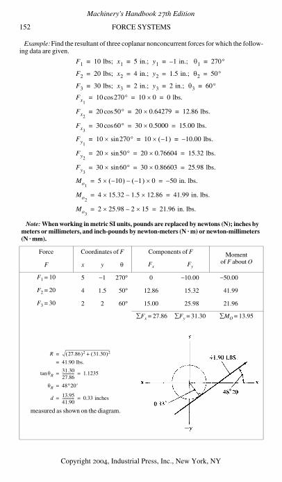
Example:Find the resultant of three coplanar nonconcurrent forces for which the follow-ing data are given.
Note: When working in metric SI units, pounds are replaced by newtons (N); inches by meters or millimeters, and inch-pounds by newton-meters (N · m) or newton-millimeters (N · mm).
Force Coordinates of F Components of F Momentof F about OF x y θ Fx Fy
F1 = 10 5 −1 270° 0 −10.00 −50.00
F2 = 20 4 1.5 50° 12.86 15.32 41.99
F3 = 30 2 2 60° 15.00 25.98 21.96
∑Fx = 27.86 ∑Fy = 31.30 ∑MO = 13.95
measured as shown on the diagram.
F1 10 lbs; x1 5 in.; y1 1– in.; θ1 270°= = = =
F2 20 lbs; x2 4 in.; y2 1.5 in.; θ2 50°= = = =
F3 30 lbs; x3 2 in.; y3 2 in.; θ3 60°= = = =
Fx110 270°cos 10 0× 0 lbs.= = =
Fx220 50°cos 20 0.64279× 12.86 lbs.= = =
Fx330 60°cos 30 0.5000× 15.00 lbs.= = =
Fy110 270sin °× 10 1–( )× 10.00– lbs.= = =
Fy220 50sin °× 20 0.76604× 15.32 lbs.= = =
Fy330 60sin °× 30 0.86603× 25.98 lbs.= = =
Mo15 10–( )× 1–( )– 0× 50– in. lbs.= =
Mo24 15.32× 1.5– 12.86× 41.99 in. lbs.= =
Mo32 25.98× 2– 15× 21.96 in. lbs.= =
R 27.86( )2 31.30( )2+=
41.90= lbs.
θtan R31.3027.86------------- 1.1235= =
θR 48°20 ′=
d 13.9541.90------------- 0.33 inches= =
Machinery's Handbook 27th Edition
Copyright 2004, Industrial Press, Inc., New York, NY
FORCE SYSTEMS 153
Algebraic Solution of Force Systems — Forces Not in Same Plane
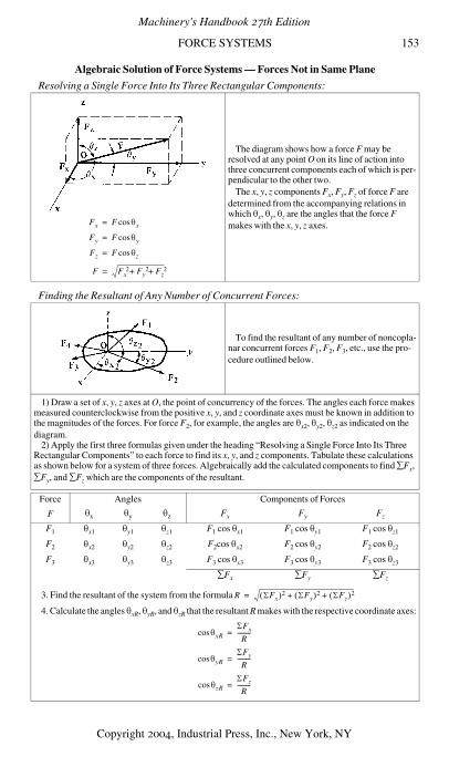
Resolving a Single Force Into Its Three Rectangular Components:
Finding the Resultant of Any Number of Concurrent Forces:
The diagram shows how a force F may be resolved at any point O on its line of action into three concurrent components each of which is per-pendicular to the other two.
The x, y, z components Fx, Fy, Fz of force F are determined from the accompanying relations in which θx, θy, θz are the angles that the force F makes with the x, y, z axes.
To find the resultant of any number of noncopla-nar concurrent forces F1, F2, F3, etc., use the pro-cedure outlined below.
1) Draw a set of x, y, z axes at O, the point of concurrency of the forces. The angles each force makes measured counterclockwise from the positive x, y, and z coordinate axes must be known in addition to the magnitudes of the forces. For force F2, for example, the angles are θx2, θy2, θz2 as indicated on the diagram.
2) Apply the first three formulas given under the heading “Resolving a Single Force Into Its Three Rectangular Components” to each force to find its x, y, and z components. Tabulate these calculations as shown below for a system of three forces. Algebraically add the calculated components to find ∑Fx, ∑Fy, and ∑Fz which are the components of the resultant.
Force Angles Components of Forces
F θx θy θz Fx Fy Fz
F1 θx1 θy1 θz1 F1 cos θx1 F1 cos θy1 F1 cos θz1
F2 θx2 θy2 θz2 F2cos θx2 F2 cos θy2 F2 cos θz2
F3 θx3 θy3 θz3 F3 cos θx3 F3 cos θy3 F3 cos θz3
∑Fx ∑Fy ∑Fz
3. Find the resultant of the system from the formula
4. Calculate the angles θxR, θyR, and θzR that the resultant R makes with the respective coordinate axes:
Fx F θxcos=
Fy F θycos=
Fz F θzcos=
F Fx2 Fy
2 Fz2+ +=
R ΣFx( )2 ΣFy( )2 ΣFz( )2+ +=
θcos xR
ΣFx
R---------=
θcos yR
ΣFy
R---------=
θcos zR
ΣFz
R---------=
Machinery's Handbook 27th Edition
Copyright 2004, Industrial Press, Inc., New York, NY
154 FORCE SYSTEMS
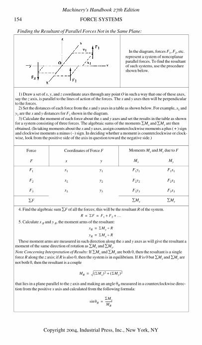
Finding the Resultant of Parallel Forces Not in the Same Plane:
In the diagram, forces F1, F2, etc. represent a system of noncoplanar parallel forces. To find the resultant of such systems, use the procedure shown below.
1) Draw a set of x, y, and z coordinate axes through any point O in such a way that one of these axes, say the z axis, is parallel to the lines of action of the forces. The x and y axes then will be perpendicular to the forces.
2) Set the distances of each force from the x and y axes in a table as shown below. For example, x1 and y1 are the x and y distances for F1 shown in the diagram.
3) Calculate the moment of each force about the x and y axes and set the results in the table as shown for a system consisting of three forces. The algebraic sums of the moments ∑Mx and ∑My are then obtained. (In taking moments about the x and y axes, assign counterclockwise moments a plus ( + ) sign and clockwise moments a minus (−) sign. In deciding whether a moment is counterclockwise or clock-wise, look from the positive side of the axis in question toward the negative side.)
Force Coordinates of Force F Moments Mx and My due to F
F x y Mx My
F1 x1 y1 F1y1 F1x1
F2 x2 y2 F2y2 F2x2
F3 x3 y3 F3y3 F3x3
∑F ∑Mx ∑My
4. Find the algebraic sum ∑F of all the forces; this will be the resultant R of the system.
5. Calculate x R and y R, the moment arms of the resultant:
These moment arms are measured in such direction along the x and y axes as will give the resultant a moment of the same direction of rotation as ∑Mx and ∑My.Note Concerning Interpretation of Results: If ∑Mx and ∑My are both 0, then the resultant is a single force R along the z axis; if R is also 0, then the system is in equilibrium. If R is 0 but ∑Mx and ∑My are not both 0, then the resultant is a couple
that lies in a plane parallel to the z axis and making an angle θR measured in a counterclockwise direc-tion from the positive x axis and calculated from the following formula:
R ΣF F1 F2 …+ += =
xR ΣMy R÷=
yR ΣMx R÷=
MR ΣMx( )2 ΣMy( )2+=
θsin R
ΣMx
MR-----------=
Machinery's Handbook 27th Edition
Copyright 2004, Industrial Press, Inc., New York, NY
FORCE SYSTEMS 155
Finding the Resultant of Nonparallel Forces Not Meeting at a Common Point:
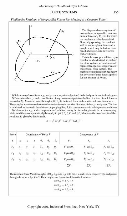
The diagram shows a system of noncoplanar, nonparallel, noncon-current forces F1, F2, etc. for which the resultant is to be determined. Generally speaking, the resultant will be a noncoplanar force and a couple which may be further com-bined, if desired, into two forces that are skewed.
This is the most general force sys-tem that can be devised, so each of the other systems so far described represents a special, simpler case of this general force system. The method of solution described below for a system of three forces applies for any number of forces.
1) Select a set of coordinate x, y, and z axes at any desired point O in the body as shown in the diagram.2) Determine the x, y, and z coordinates of any convenient point on the line of action of each force as
shown for F2. Also determine the angles, θx, θy, θz that each force makes with each coordinate axis. These angles are measured counterclockwise from the positive direction of the x, y, and z axes. The data is tabulated, as shown in the table accompanying Step 3, for convenient use in subsequent calculations.
3) Calculate the x, y, and z components of each force using the formulas given in the accompanying table. Add these components algebraically to get ∑Fx, ∑Fy and ∑Fz which are the components of the resultant, R, given by the formula,
Force Coordinates of Force F Components of F
F x y z θx θy θz Fx Fy Fz
F1 x1 y1 z1 θx1 θy1 θz1 F1 cos θx1 F1 cos θy1 F1 cos θz1
F2 x2 y2 z2 θx2 θy2 θz2 F2 cos θx2 F2 cos θy2 F2 cos θz2
F3 x3 y3 z3 θx3 θy3 θz3 F3 cos θx3 F3 cos θy3 F3 cos θz3
∑Fx ∑Fy ∑Fz
The resultant force R makes angles of θxR, θyR, and θzR with the x, y, and z axes, respectively, and passes through the selected point O. These angles are determined from the formulas,
R ΣFx( )2 ΣFy( )2 ΣFz( )2+ +=
θcos xR ΣFx R÷=
θcos yR ΣFy R÷=
θcos zR ΣFz R÷=
Machinery's Handbook 27th Edition
Copyright 2004, Industrial Press, Inc., New York, NY
156 FORCE SYSTEMS
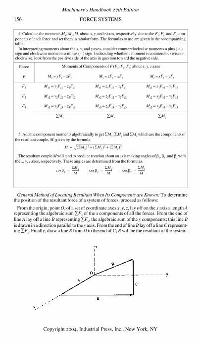
General Method of Locating Resultant When Its Components are Known: To determinethe position of the resultant force of a system of forces, proceed as follows:
From the origin, point O, of a set of coordinate axes x, y, z, lay off on the x axis a length Arepresenting the algebraic sum ∑Fx of the x components of all the forces. From the end ofline A lay off a line B representing ∑Fy, the algebraic sum of the y components; this line Bis drawn in a direction parallel to the y axis. From the end of line B lay off a line C represent-ing ∑Fz. Finally, draw a line R from O to the end of C; R will be the resultant of the system.
4. Calculate the moments Mx, My, Mz about x, y, and z axes, respectively, due to the Fx, Fy, and Fz com-ponents of each force and set them in tabular form. The formulas to use are given in the accompanying table.
In interpreting moments about the x, y, and z axes, consider counterclockwise moments a plus ( + ) sign and clockwise moments a minus (− ) sign. In deciding whether a moment is counterclockwise or clockwise, look from the positive side of the axis in question toward the negative side.
Force Moments of Components of F (Fx, Fy, Fz) about x, y, z axes
F Mx = yFz − zFy My = zFx − xFz Mz = xFy − yFx
F1 Mx1 = y1Fz1 − z1Fy1 My1 = z1Fx1 − x1Fz1 Mz1 = x1Fy1 − y1Fx1
F2 Mx2 = y2Fz2 − z2Fy2 My2 = z2Fx2 − x2Fz2 Mz2 = x2Fy2 − y2Fx2
F3 Mx3 = y3Fz3 − z3Fy3 My3 = z3Fx3 − x3Fz3 Mz3 = x3Fy3 − y3Fx3
∑Mx ∑My ∑Mz
5. Add the component moments algebraically to get ∑Mx, ∑My and ∑Mz which are the components of the resultant couple, M, given by the formula,
The resultant couple M will tend to produce rotation about an axis making angles of βx, βy, and βz with the x, y, z axes, respectively. These angles are determined from the formulas,
M ΣMx( )2 ΣMy( )2 ΣMz( )2+ +=
βxcosΣMx
M-----------= βycos
ΣMy
M-----------= βzcos
ΣMz
M----------=
Machinery's Handbook 27th Edition
Copyright 2004, Industrial Press, Inc., New York, NY
FRICTION 157
Friction
Properties of Friction.—Friction is the resistance to motion that takes place when onebody is moved upon another, and is generally defined as “that force which acts betweentwo bodies at their surface of contact, so as to resist their sliding on each other.” Accordingto the conditions under which sliding occurs, the force of friction, F, bears a certain relationto the force between the two bodies called the normal force N. The relation between forceof friction and normal force is given by the coefficient of friction, generally denoted by theGreek letter µ. Thus:
Example:A body weighing 28 pounds rests on a horizontal surface. The force required tokeep it in motion along the surface is 7 pounds. Find the coefficient of friction.
If a body is placed on an inclined plane, the friction between the body and the plane willprevent it from sliding down the inclined surface, provided the angle of the plane with thehorizontal is not too great. There will be a certain angle, however, at which the body willjust barely be able to remain stationary, the frictional resistance being very nearly over-come by the tendency of the body to slide down. This angle is termed the angle of repose,and the tangent of this angle equals the coefficient of friction. The angle of repose is fre-quently denoted by the Greek letter θ. Thus, µ = tan θ.
A greater force is required to start a body moving from a state of rest than to merely keepit in motion, because the friction of rest is greater than the friction of motion.Laws of Friction.—The laws of friction for unlubricated or dry surfaces are summarizedin the following statements.
1) For low pressures (normal force per unit area) the friction is directly proportional tothe normal force between the two surfaces. As the pressure increases, the friction does notrise proportionally; but when the pressure becomes abnormally high, the friction increasesat a rapid rate until seizing takes place.
2) The friction both in its total amount and its coefficient is independent of the areas incontact, so long as the normal force remains the same. This is true for moderate pressuresonly. For high pressures, this law is modified in the same way as in the first case.
3) At very low velocities the friction is independent of the velocity of rubbing. As thevelocities increase, the friction decreases.
Lubricated Surfaces: For well lubricated surfaces, the laws of friction are considerablydifferent from those governing dry or poorly lubricated surfaces.
1) The frictional resistance is almost independent of the pressure (normal force per unitarea) if the surfaces are flooded with oil.
2) The friction varies directly as the speed, at low pressures; but for high pressures thefriction is very great at low velocities, approaching a minimum at about two feet per secondlinear velocity, and afterwards increasing approximately as the square root of the speed.
3) For well lubricated surfaces the frictional resistance depends, to a very great extent, onthe temperature, partly because of the change in the viscosity of the oil and partly because,for a journal bearing, the diameter of the bearing increases with the rise of temperaturemore rapidly than the diameter of the shaft, thus relieving the bearing of side pressure.
4) If the bearing surfaces are flooded with oil, the friction is almost independent of thenature of the material of the surfaces in contact. As the lubrication becomes less ample, thecoefficient of friction becomes more dependent upon the material of the surfaces.Influence of Friction on the Efficiency of Small Machine Elements.—Fr i c t i onbetween machine parts lowers the efficiency of a machine. Average values of the effi-ciency, in per cent, of the most common machine elements when carefully made are ordi-
F µ N×= and µFN----=
µFN---- 7
28------ 0.25= = =
Machinery's Handbook 27th Edition
Copyright 2004, Industrial Press, Inc., New York, NY
158 FRICTION
nary bearings, 95 to 98; roller bearings, 98; ball bearings, 99; spur gears with cut teeth,including bearings, 99; bevel gears with cut teeth, including bearings, 98; belting, from 96to 98; high-class silent power transmission chain, 97 to 99; roller chains, 95 to 97.
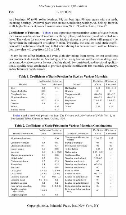
Coefficients of Friction.—Tables 1 and 2 provide representative values of static frictionfor various combinations of materials with dry (clean, unlubricated) and lubricated sur-faces. The values for static or breakaway friction shown in these tables will generally behigher than the subsequent or sliding friction. Typically, the steel-on-steel static coeffi-cient of 0.8 unlubricated will drop to 0.4 when sliding has been initiated; with oil lubrica-tion, the value will drop from 0.16 to 0.03.
Many factors affect friction, and even slight deviations from normal or test conditionscan produce wide variations. Accordingly, when using friction coefficients in design cal-culations, due allowance or factors of safety should be considered, and in critical applica-tions, specific tests conducted to provide specific coefficients for material, geometry,and/or lubricant combinations.
Table 1. Coefficients of Static Friction for Steel on Various Materials
Tables 1 and 2 used with permission from The Friction and Lubrication of Solids, Vol. 1, byBowden and Tabor, Clarendon Press, Oxford, 1950.
Table 2. Coefficients of Static Friction for Various Materials Combinations
Material
Coefficient of Friction, µ
Material
Coefficient of Friction, µ
Clean Lubricated Clean Lubricated
Steel 0.8 0.16 Hard carbon 0.14 0.11–0.14Copper-lead alloy 0.22 … Graphite 0.1 0.1Phosphor-bronze 0.35 … Tungsten carbide 0.4–0.6 0.1–0.2Aluminum-bronze 0.45 … Plexiglas 0.4–0.5 0.4–0.5Brass 0.35 0.19 Polystyrene 0.3–0.35 0.3–0.35Cast iron 0.4 0.21 Polythene 0.2 0.2Bronze … 0.16 Teflon 0.04 0.04Sintered bronze … 0.13
Material Combination
Coefficient of Friction, µ
Material Combination
Coefficient of Friction, µ
Clean Lubricated Clean Lubricated
Aluminum-aluminum 1.35 0.30 Tungsten carbide-tungsten carbide 0.2–0.25 0.12
Cadmium-cadmium 0.5 0.05 Plexiglas-Plexiglas 0.8 0.8Chromium-chromium 0.41 0.34 Polystyrene-polystyrene 0.5 0.5Copper-copper 1.0 0.08 Teflon-Teflon 0.04 0.04Iron-iron 1.0 0.15 –0.20 Nylon-nylon 0.15–0.25 …Magnesium-magnesium 0.6 0.08 Solids on rubber 1– 4 …Nickel-nickel 0.7 0.28 Wood on wood (clean) 0.25–0.5 …Platinum-platinum 1.2 0.25 Wood on wood (wet) 0.2 …Silver-silver 1.4 0.55 Wood on metals (clean) 0.2–0.6 …Zinc-zinc 0.6 0.04 Wood on metals (wet) 0.2 …Glass-glass 0.9–1.0 0.1–0.6 Brick on wood 0.6 …Glass-metal 0.5–0.7 0.2–0.3 Leather on wood 0.3–0.4 …Diamond-diamond 0.1 0.05–0.1 Leather on metal (clean) 0.6 …Diamond-metal 0.1–0.15 0.1 Leather on metal (wet) 0.4 …Sapphire-sapphire 0.2 0.2 Leather on metal (greasy) 0.2 …Hard carbon on carbon 0.16 0.12–0.14 Brake material on cast iron 0.4 …Graphite-graphite
(in vacuum) 0.5–0.8 … Brake material on cast iron (wet) 0.2 …
Graphite-graphite 0.1 0.1
Machinery's Handbook 27th Edition
Copyright 2004, Industrial Press, Inc., New York, NY
ROLLING FRICTION 159
Rolling Friction.—When a body rolls on a surface, the force resisting the motion istermed rolling friction or rolling resistance. Let W = total weight of rolling body or load onwheel, in pounds; r = radius of wheel, in inches; f = coefficient of rolling resistance, ininches. Then: resistance to rolling, in pounds = (W × f) ÷ r.
The coefficient of rolling resistance varies with the conditions. For wood on wood it maybe assumed as 0.06 inch; for iron on iron, 0.02 inch; iron on granite, 0.085 inch; iron onasphalt, 0.15 inch; and iron on wood, 0.22 inch.
The coefficient of rolling resistance, f, is in inches and is not the same as the sliding orstatic coefficient of friction given in Tables 1 and 2, which is a dimensionless ratio betweenfrictional resistance and normal load. Various investigators are not in close agreement onthe true values for these coefficients and the foregoing values should only be used for theapproximate calculation of rolling resistance.
Mechanisms
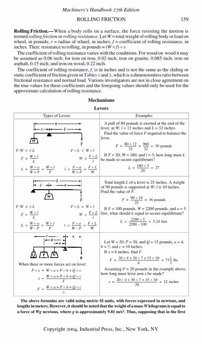
Levers
The above formulas are valid using metric SI units, with forces expressed in newtons, andlengths in meters. However, it should be noted that the weight of a mass W kilograms is equal toa force of Wg newtons, where g is approximately 9.81 m/s2. Thus, supposing that in the first
Types of Levers Examples
A pull of 80 pounds is exerted at the end of the lever, at W; l = 12 inches and L = 32 inches.
Find the value of force F required to balance the lever.
If F = 20; W = 180; and l = 3; how long must L be made to secure equilibrium?
Total length L of a lever is 25 inches. A weight of 90 pounds is supported at W; l is 10 inches. Find the value of F.
If F = 100 pounds, W = 2200 pounds, and a = 5 feet, what should L equal to secure equilibrium?
When three or more forces act on lever:
Let W = 20, P = 30, and Q = 15 pounds; a = 4,b = 7, and c = 10 inches.
If x = 6 inches, find F.
Assuming F = 20 pounds in the example above, how long must lever arm x be made?
F:W l:L= F L× W l×=
F W l×
L------------= W F L×
l-------------=
L W a×
W F+--------------- W l×
F------------= = l F a×
W F+--------------- F L×
W-------------= =
F 80 12×
32------------------ 960
32--------- 30 pounds= = =
L 180 3×
20------------------ 27= =
F:W l:L= F L× W l×=
F W l×
L------------= W F L×
l-------------=
L W a×
W F–-------------- W l×
F------------= = l F a×
W F–-------------- F L×
W-------------= =
F 90 10×
25------------------ 36 pounds= =
L 2200 5×
2200 100–--------------------------- 5.24 feet= =
F x× W a× P+ b× Q+ c×=
x W a× P+ b× Q+ c×
F-----------------------------------------------------=
F W a× P+ b× Q+ c×
x-----------------------------------------------------=
F 20 4× 30+ 7× 15+ 10×
6------------------------------------------------------------- 731
3--- lbs= =
x 20 4× 30+ 7× 15+ 10×
20------------------------------------------------------------- 22 inches= =
Machinery's Handbook 27th Edition
Copyright 2004, Industrial Press, Inc., New York, NY
160 SIMPLE MECHANISMS
example l = 0.4 m, L = 1.2 m, and W = 30 kg, then the weight of W is 30g newtons, so that the
force F required to balance the lever is
This force could be produced by suspending a mass of 10 kg at F.
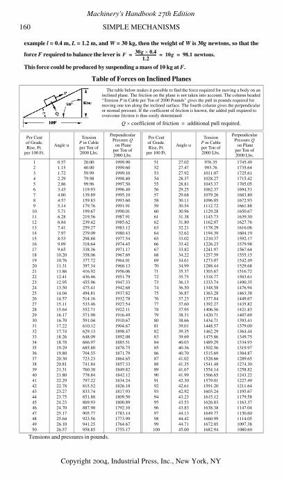
Table of Forces on Inclined Planes
Tensions and pressures in pounds.
The table below makes it possible to find the force required for moving a body on an inclined plane. The friction on the plane is not taken into account. The column headed “Tension P in Cable per Ton of 2000 Pounds” gives the pull in pounds required for moving one ton along the inclined surface. The fourth column gives the perpendicular or normal pressure. If the coefficient of friction is known, the added pull required to overcome friction is thus easily determined:
Per Centof Grade.Rise, Ft.
per 100 Ft.
Angle α
TensionP in Cableper Ton of2000 Lbs.
PerpendicularPressure Q on Planeper Ton of2000 Lbs.
Per Centof Grade.Rise, Ft.
per 100 Ft.
Angle α
TensionP in Cableper Ton of2000 Lbs.
PerpendicularPressure Q on Planeper Ton of2000 Lbs.
1 0.57 20.00 1999.90 51 27.02 976.35 1745.492 1.15 40.00 1999.60 52 27.47 993.76 1735.643 1.72 59.99 1999.10 53 27.92 1011.07 1725.614 2.29 79.98 1998.40 54 28.37 1028.27 1715.425 2.86 99.96 1997.50 55 28.81 1045.37 1705.056 3.43 119.93 1996.40 56 29.25 1062.37 1694.517 4.00 139.89 1995.10 57 29.68 1079.26 1683.808 4.57 159.83 1993.60 58 30.11 1096.05 1672.939 5.14 179.76 1991.91 59 30.54 1112.72 1661.88
10 5.71 199.67 1990.01 60 30.96 1129.28 1650.6711 6.28 219.56 1987.91 61 31.38 1145.73 1639.3012 6.84 239.42 1985.62 62 31.80 1162.07 1627.7613 7.41 259.27 1983.12 63 32.21 1178.29 1616.0614 7.97 279.09 1980.43 64 32.62 1194.39 1604.1915 8.53 298.88 1977.54 65 33.02 1210.37 1592.1716 9.09 318.64 1974.45 66 33.42 1226.23 1579.9817 9.65 338.36 1971.17 67 33.82 1241.97 1567.6418 10.20 358.06 1967.69 68 34.22 1257.59 1555.1519 10.76 377.72 1964.01 69 34.61 1273.07 1542.4920 11.31 397.34 1960.13 70 34.99 1288.44 1529.6821 11.86 416.92 1956.06 71 35.37 1303.67 1516.7222 12.41 436.46 1951.79 72 35.75 1318.77 1503.6123 12.95 455.96 1947.33 73 36.13 1333.74 1490.3524 13.50 475.41 1942.68 74 36.50 1348.58 1476.9425 14.04 494.81 1937.82 75 36.87 1363.28 1463.3826 14.57 514.16 1932.78 76 37.23 1377.84 1449.6727 15.11 533.46 1927.54 77 37.60 1392.27 1435.8228 15.64 552.71 1922.11 78 37.95 1406.56 1421.8329 16.17 571.90 1916.49 79 38.31 1420.71 1407.6930 16.70 591.04 1910.67 80 38.66 1434.71 1393.4131 17.22 610.12 1904.67 81 39.01 1448.57 1379.0032 17.74 629.13 1898.47 82 39.35 1462.29 1364.4433 18.26 648.09 1892.08 83 39.69 1475.86 1349.7534 18.78 666.97 1885.51 84 40.03 1489.29 1334.9335 19.29 685.80 1878.75 85 40.36 1502.56 1319.9736 19.80 704.55 1871.79 86 40.70 1515.69 1304.8737 20.30 723.23 1864.65 87 41.02 1528.66 1289.6538 20.81 741.84 1857.33 88 41.35 1541.48 1274.3039 21.31 760.38 1849.82 89 41.67 1554.14 1258.8240 21.80 778.84 1842.12 90 41.99 1566.65 1243.2241 22.29 797.22 1834.24 91 42.30 1579.01 1227.4942 22.78 815.52 1826.18 92 42.61 1591.20 1211.6443 23.27 833.74 1817.93 93 42.92 1603.24 1195.6744 23.75 851.88 1809.50 94 43.23 1615.12 1179.5845 24.23 869.93 1800.89 95 43.53 1626.83 1163.3746 24.70 887.90 1792.10 96 43.83 1638.38 1147.0447 25.17 905.77 1783.14 97 44.13 1649.77 1130.6048 25.64 923.56 1773.99 98 44.42 1660.99 1114.0549 26.10 941.25 1764.67 99 44.71 1672.05 1097.3850 26.57 958.85 1755.17 100 45.00 1682.94 1080.60
F 30g 0.4×
1.2----------------------- 10g 98.1 newtons.= = =
Q coefficient of friction× additional pull required.=
Machinery's Handbook 27th Edition
Copyright 2004, Industrial Press, Inc., New York, NY

SIMPLE MECHANISMS 161
Inclined Plane—WedgeW = weight of body
Neglecting friction:
If friction is taken into account, then
Force P to pull body up is:
Force P1 to pull body down is:
Force P2 to hold body stationary:
in which µ is the coefficient of friction.
W = weight of body W = weight of body
Neglecting friction: With friction: Neglecting friction: With friction:
Neglecting friction:
With friction:Coefficient of friction = µ.
Neglecting friction:
With friction:Coefficient of friction = µ = tan φ.
Force Moving Body on Horizontal Plane.—F tends to move B along line CD; Q is the component which actually moves B; P is the pressure, due to F, of the body on CD.
P W hl---× W αsin×= =
W P lh---×
Pαsin
----------- P cosecα×= = =
Q W bl---× W αcos×= =
P W µ αcos αsin+( )=
P1 W µ αcos αsin–( )=
P2 W αsin µ αcos–( )=
P W αsinβcos
------------×=
W P βcosαsin
------------×=
Q W α β+( )cosβcos
---------------------------×=
Coefficient of frictionµ= φtan=
P W α φ+( )sinβ φ–( )cos
--------------------------×=
P W hb---× W αtan×= =
W P bh---× P αcot×= =
Q Wαcos
------------ W αsec×= =
Coefficient of frictionµ= φtan=
P W α φ+( )tan=
P 2Q bl---× 2Q αsin×= =
Q P l2b------×
12---P cosecα×= =
P 2Q µ αcos αsin+( )=
P 2Q bh---× 2Q αtan×= =
Q P h2b------×
12---P αcot×= =
P 2Q α φ+( )tan=
Q F αcos×= P F2 Q2–=
Machinery's Handbook 27th Edition
Copyright 2004, Industrial Press, Inc., New York, NY
162 SIMPLE MECHANISMS
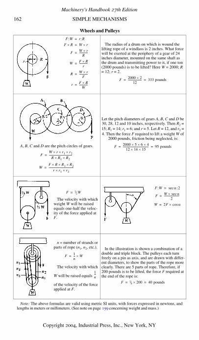
Wheels and Pulleys
Note: The above formulas are valid using metric SI units, with forces expressed in newtons, andlengths in meters or millimeters. (See note on page 159 concerning weight and mass.)
The radius of a drum on which is wound the lifting rope of a windlass is 2 inches. What force will be exerted at the periphery of a gear of 24 inches diameter, mounted on the same shaft as the drum and transmitting power to it, if one ton (2000 pounds) is to be lifted? Here W = 2000; R = 12; r = 2.
A, B, C and D are the pitch circles of gears.
Let the pitch diameters of gears A, B, C and D be 30, 28, 12 and 10 inches, respectively. Then R2 = 15; R1 = 14; r1 = 6; and r = 5. Let R = 12, and r2 = 4. Then the force F required to lift a weight W of
2000 pounds, friction being neglected, is:
The velocity with which weight W will be raised equals one-half the veloc-ity of the force applied at F.
n = number of strands or parts of rope (n1, n2, etc.).
The velocity with which
W will be raised equals
of the velocity of the force applied at F.
In the illustration is shown a combination of a double and triple block. The pulleys each turn freely on a pin as axis, and are drawn with differ-ent diameters, to show the parts of the rope more clearly. There are 5 parts of rope. Therefore, if 200 pounds is to be lifted, the force F required at the end of the rope is:
F:W r:R=
F R× W r×=
F W r×
R-------------=
W F R×
r-------------=
R W r×
F-------------=
r F R×
W-------------=
F 2000 2×
12--------------------- 333 pounds= =
FW r× r1× r2×
R R1× R2×-----------------------------------=
WF R× R1× R2×
r r1× r2×--------------------------------------=
F 2000 5× 6× 4×
12 14× 15×--------------------------------------- 95 pounds= =
F 1⁄2W=F:W αsec :2=
F W αsec×
2-----------------------=
W 2F αcos×=
F 1n--- W×=
1n---
F 1⁄5 200× 40 pounds= =
Machinery's Handbook 27th Edition
Copyright 2004, Industrial Press, Inc., New York, NY
SIMPLE MECHANISMS 163
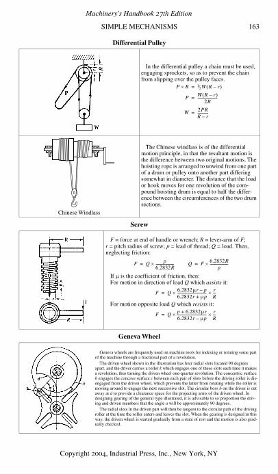
Differential Pulley
Screw
Geneva Wheel
In the differential pulley a chain must be used, engaging sprockets, so as to prevent the chain from slipping over the pulley faces.
Chinese Windlass
The Chinese windlass is of the differential motion principle, in that the resultant motion is the difference between two original motions. The hoisting rope is arranged to unwind from one part of a drum or pulley onto another part differing somewhat in diameter. The distance that the load or hook moves for one revolution of the com-pound hoisting drum is equal to half the differ-ence between the circumferences of the two drum sections.
F = force at end of handle or wrench; R = lever-arm of F; r = pitch radius of screw; p = lead of thread; Q = load. Then, neglecting friction:
If µ is the coefficient of friction, then:For motion in direction of load Q which assists it:
For motion opposite load Q which resists it:
Geneva wheels are frequently used on machine tools for indexing or rotating some part of the machine through a fractional part of a revolution.
The driven wheel shown in the illustration has four radial slots located 90 degrees apart, and the driver carries a roller k which engages one of these slots each time it makes a revolution, thus turning the driven wheel one-quarter revolution. The concentric surface b engages the concave surface c between each pair of slots before the driving roller is dis-engaged from the driven wheel, which prevents the latter from rotating while the roller is moving around to engage the next successive slot. The circular boss b on the driver is cut away at d to provide a clearance space for the projecting arms of the driven wheel. In designing gearing of the general type illustrated, it is advisable to so proportion the driv-ing and driven members that the angle a will be approximately 90 degrees.
The radial slots in the driven part will then be tangent to the circular path of the driving roller at the time the roller enters and leaves the slot. When the gearing is designed in this way, the driven wheel is started gradually from a state of rest and the motion is also grad-ually checked.
P R× 1⁄2W R r–( )=
P W R r–( )
2R----------------------=
W 2PRR r–------------=
F Q p6.2832R--------------------×= Q F 6.2832R
p--------------------×=
F Q 6.2832µr p–6.2832r µp+--------------------------------×
rR---×=
F Q p 6.2832µr+6.2832r µp–--------------------------------×
rR---×=
Machinery's Handbook 27th Edition
Copyright 2004, Industrial Press, Inc., New York, NY
164 SIMPLE MECHANISMS
Toggle-joints with Equal Arms
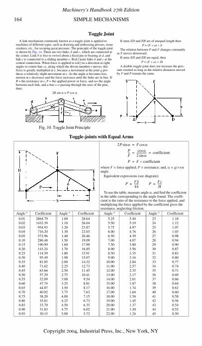
Toggle JointA link mechanism commonly known as a toggle joint is applied to
machines of different types, such as drawing and embossing presses, stone crushers, etc., for securing great pressure. The principle of the toggle joint is shown by Fig. 10. There are two links, b and c, which are connected at the center. Link b is free to swivel about a fixed pin or bearing at d, and link e is connected to a sliding member e. Rod f joins links b and c at the central connection. When force is applied to rod f in a direction at right angles to center-line xx, along which the driven member e moves, this force is greatly multiplied at e, because a movement at the joint g pro-duces a relatively slight movement at e. As the angle α becomes less, motion at e decreases and the force increases until the links are in line. If R = the resistance at e, P = the applied power or force, and α= the angle between each link, and a line x–x passing through the axes of the pins, then:
2R sin α = P cos α
If arms ED and EH are of unequal length thenP = (F × a) ÷ b
The relation between P and F changes constantly as F moves downward.
If arms ED and EH are equal, thenP = (F × a) ÷ 2h
A double toggle-joint does not increase the pres-sure exerted so long as the relative distances moved by F and P remain the same.
Fig. 10. Toggle Joint Principle
where F = force applied; P = resistance; and, α = g ivenangle.
Equivalent expressions (see diagram):
To use the table, measure angle α, and find the coefficient in the table corresponding to the angle found. The coeffi-cient is the ratio of the resistance to the force applied, and multiplying the force applied by the coefficient gives the resistance, neglecting friction.
Angle ° Coefficient Angle ° Coefficient Angle ° Coefficient Angle ° Coefficient
0.01 2864.79 1.00 28.64 5.25 5.44 23 1.180.02 1432.39 1.10 26.04 5.50 5.19 24 1.120.03 954.93 1.20 23.87 5.75 4.97 25 1.070.04 716.20 1.30 22.03 6.00 4.76 26 1.030.05 572.96 1.40 20.46 6.50 4.39 27 0.980.10 286.48 1.50 19.09 7.00 4.07 28 0.940.15 190.99 1.60 17.90 7.50 3.80 29 0.900.20 143.24 1.70 16.85 8.00 3.56 30 0.870.25 114.59 1.80 15.91 8.50 3.35 31 0.830.30 95.49 1.90 15.07 9.00 3.16 32 0.800.35 81.85 2.00 14.32 10.00 2.84 33 0.770.40 71.62 2.25 12.73 11.00 2.57 34 0.740.45 63.66 2.50 11.45 12.00 2.35 35 0.710.50 57.29 2.75 10.41 13.00 2.17 36 0.690.55 52.09 3.00 9.54 14.00 2.01 37 0.660.60 47.74 3.25 8.81 15.00 1.87 38 0.640.65 44.07 3.50 8.17 16.00 1.74 39 0.620.70 40.92 3.75 7.63 17.00 1.64 40 0.600.75 38.20 4.00 7.15 18.00 1.54 41 0.580.80 35.81 4.25 6.73 19.00 1.45 42 0.560.85 33.70 4.50 6.35 20.00 1.37 43 0.540.90 31.83 4.75 6.02 21.00 1.30 44 0.520.95 30.15 5.00 5.72 22.00 1.24 45 0.50
2P αsin F αcos=
PF--- αcos
2 αsin--------------- coefficient= =
P F coefficient×=
P FS4h-------= P Fs
H------=
Machinery's Handbook 27th Edition
Copyright 2004, Industrial Press, Inc., New York, NY
PENDULUMS 165
Pendulums
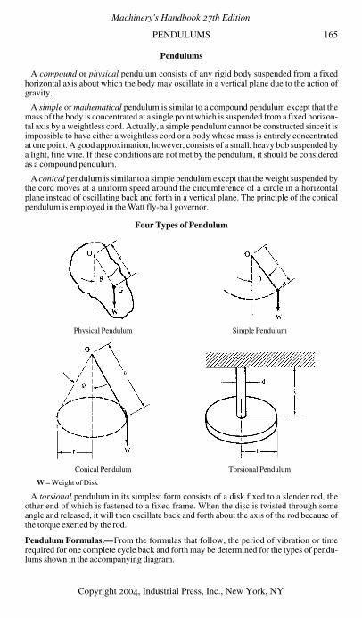
A compound or physical pendulum consists of any rigid body suspended from a fixedhorizontal axis about which the body may oscillate in a vertical plane due to the action ofgravity.
A simple or mathematical pendulum is similar to a compound pendulum except that themass of the body is concentrated at a single point which is suspended from a fixed horizon-tal axis by a weightless cord. Actually, a simple pendulum cannot be constructed since it isimpossible to have either a weightless cord or a body whose mass is entirely concentratedat one point. A good approximation, however, consists of a small, heavy bob suspended bya light, fine wire. If these conditions are not met by the pendulum, it should be consideredas a compound pendulum.
A conical pendulum is similar to a simple pendulum except that the weight suspended bythe cord moves at a uniform speed around the circumference of a circle in a horizontalplane instead of oscillating back and forth in a vertical plane. The principle of the conicalpendulum is employed in the Watt fly-ball governor.
Four Types of Pendulum
W = Weight of Disk
A torsional pendulum in its simplest form consists of a disk fixed to a slender rod, theother end of which is fastened to a fixed frame. When the disc is twisted through someangle and released, it will then oscillate back and forth about the axis of the rod because ofthe torque exerted by the rod.
Pendulum Formulas.—From the formulas that follow, the period of vibration or timerequired for one complete cycle back and forth may be determined for the types of pendu-lums shown in the accompanying diagram.
Physical Pendulum Simple Pendulum
Conical Pendulum Torsional Pendulum
Machinery's Handbook 27th Edition
Copyright 2004, Industrial Press, Inc., New York, NY
166 PENDULUMS
For a simple pendulum,
(1)
where T = period in seconds for one complete cycle; g = acceleration due to gravity = 32.17feet per second per second (approximately); and l is the length of the pendulum in feet asshown on the accompanying diagram.
For a physical or compound pendulum,
(2)
where k0 = radius of gyration of the pendulum about the axis of rotation, in feet, and r is thedistance from the axis of rotation to the center of gravity, in feet.
The metric SI units that can be used in the two above formulas are T = seconds; g =approximately 9.81 meters per second squared, which is the value for accelerationdue to gravity; l = the length of the pendulum in meters; k0 = the radius of gyration inmeters, and r = the distance from the axis of rotation to the center of gravity, inmeters.
Formulas (1) and (2) are accurate when the angle of oscillation θ shown in the diagram isvery small. For θ equal to 22 degrees, these formulas give results that are too small by 1 percent; for θ equal to 32 degrees, by 2 per cent.
For a conical pendulum, the time in seconds for one revolution is:
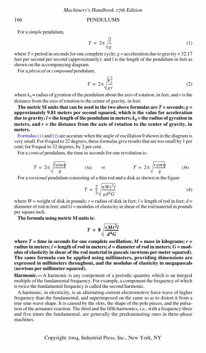
For a torsional pendulum consisting of a thin rod and a disk as shown in the figure
(4)
where W = weight of disk in pounds; r = radius of disk in feet; l = length of rod in feet; d =diameter of rod in feet; and G = modulus of elasticity in shear of the rod material in poundsper square inch.
The formula using metric SI units is:
where T = time in seconds for one complete oscillation; M = mass in kilograms; r =radius in meters; l = length of rod in meters; d = diameter of rod in meters; G = mod-ulus of elasticity in shear of the rod material in pascals (newtons per meter squared).The same formula can be applied using millimeters, providing dimensions areexpressed in millimeters throughout, and the modulus of elasticity in megapascals(newtons per millimeter squared).Harmonic.—A harmonic is any component of a periodic quantity which is an integralmultiple of the fundamental frequency. For example, a component the frequency of whichis twice the fundamental frequency is called the second harmonic.
A harmonic, in electricity, is an alternating-current electromotive force wave of higherfrequency than the fundamental, and superimposed on the same so as to distort it from atrue sine-wave shape. It is caused by the slots, the shape of the pole pieces, and the pulsa-tion of the armature reaction. The third and the fifth harmonics, i.e., with a frequency threeand five times the fundamental, are generally the predominating ones in three-phasemachines.
(3a) or (3b)
T 2π lg---=
T 2πko
2
gr-----=
T 2π l φcosg
--------------= T 2π r φcotg
--------------=
T 23--- πWr2l
gd4G----------------=
T 8 πMr2ld4G
----------------=
Machinery's Handbook 27th Edition
Copyright 2004, Industrial Press, Inc., New York, NY
MECHANICS 167
VELOCITY, ACCELERATION, WORK, AND ENERGY
Velocity and Acceleration
Motion is a progressive change of position of a body. Velocity is the rate of motion, thatis, the rate of change of position. When the velocity of a body is the same at every momentduring which the motion takes place, the latter is called uniform motion. When the velocityis variable and constantly increasing, the rate at which it changes is called acceleration;that is, acceleration is the rate at which the velocity of a body changes in a unit of time, asthe change in feet per second, in one second. When the motion is decreasing instead ofincreasing, it is called retarded motion, and the rate at which the motion is retarded is fre-quently called the deceleration. If the acceleration is uniform, the motion is called uni-formly accelerated motion. An example of such motion is found in that of falling bodies.Newton's Laws of Motion.—The first clear statement of the fundamental relations exist-ing between force and motion was made in the seventeenth century by Sir Isaac Newton,the English mathematician and physicist. It was put in the form of three laws, which aregiven as originally stated by Newton:
1) Every body continues in its state of rest, or uniform motion in a straight line, except inso far as it may be compelled by force to change that state.
2) Change of motion is proportional to the force applied and takes place in the directionin which that force acts.
3) To every action there is always an equal reaction; or, the mutual actions of two bodiesare always equal and oppositely directed.
Motion with Constant Velocity.—In the formulas that follow, S = distance moved; V =velocity; t = time of motion, θ = angle of rotation, and ω = angular velocity; the usual unitsfor these quantities are, respectively, feet, feet per second, seconds, radians, and radiansper second. Any other consistent set of units may be employed.
Constant Linear Velocity:
Constant Angular Velocity:
Relation between Angular Motion and Linear Motion: The relation between the angularvelocity of a rotating body and the linear velocity of a point at a distance r feet from thecenter of rotation is:
Similarly, the distance moved by the point during rotation through angle θ is:
Linear Motion with Constant Acceleration.—The relations between distance, velocity,and time for linear motion with constant or uniform acceleration are given by the formulasin the accompanying Table 1. In these formulas, the acceleration is assumed to be in thesame direction as the initial velocity; hence, if the acceleration in a particular problemshould happen to be in a direction opposite that of the initial velocity, then a should bereplaced by − a. Thus, for example, the formula Vf = Vo + at becomes Vf = Vo − at when aand Vo are opposite in direction.
Example:A car is moving at 60 mph when the brakes are suddenly locked and the carbegins to skid. If it takes 2 seconds to slow the car to 30 mph, at what rate is it being decel-erated, how long is it before the car comes to a halt, and how far will it have traveled?
The initial velocity Vo of the car is 60 mph or 88 ft/sec and the acceleration a due to brak-ing is opposite in direction to Vo, since the car is slowed to 30 mph or 44 ft/sec.
S V t×= V S t÷= t S V÷=
θ ωt= ω θ t÷= t θ ω÷=
V ft per sec( ) r ft( ) ω radians per sec( )×=
S ft( ) r ft( ) θ radians( )×=
Machinery's Handbook 27th Edition
Copyright 2004, Industrial Press, Inc., New York, NY
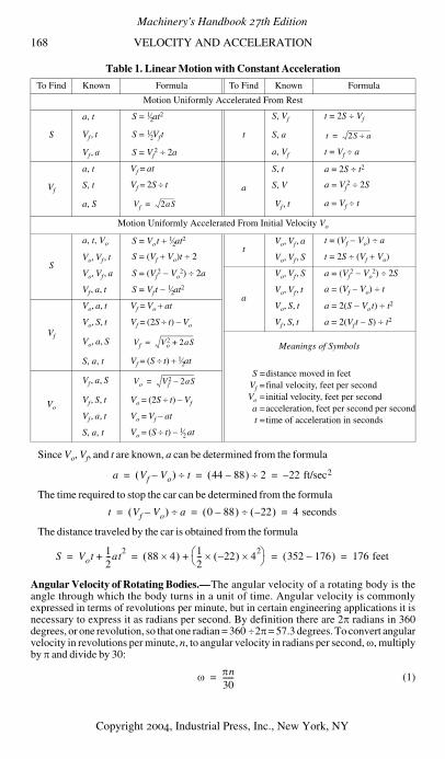
168 VELOCITY AND ACCELERATION
Since Vo, Vf, and t are known, a can be determined from the formula
The time required to stop the car can be determined from the formula
The distance traveled by the car is obtained from the formula
Angular Velocity of Rotating Bodies.—The angular velocity of a rotating body is theangle through which the body turns in a unit of time. Angular velocity is commonlyexpressed in terms of revolutions per minute, but in certain engineering applications it isnecessary to express it as radians per second. By definition there are 2π radians in 360degrees, or one revolution, so that one radian = 360 ÷2π = 57.3 degrees. To convert angularvelocity in revolutions per minute, n, to angular velocity in radians per second, ω, multiplyby π and divide by 30:
(1)
Table 1. Linear Motion with Constant Acceleration
To Find Known Formula To Find Known Formula
Motion Uniformly Accelerated From Rest
S
a, t S = 1⁄2at2
t
S, Vf t = 2S ÷ Vf
Vf , t S = 1⁄2Vft S, a
Vf , a S = Vf2 ÷ 2a a, Vf t = Vf ÷ a
Vf
a, t Vf = at
a
S, t a = 2S ÷ t2
S, t Vf = 2S ÷ t S, V a = Vf2 ÷ 2S
a, S Vf , t a = Vf ÷ t
Motion Uniformly Accelerated From Initial Velocity Vo
S
a, t, Vo S = Vot + 1⁄2at2t
Vo, Vf , a t = (Vf − Vo) ÷ a
Vo, Vf , t S = (Vf + Vo)t ÷ 2 Vo, Vf , S t = 2S ÷ (Vf + Vo)
Vo, Vf , a S = (Vf2 − Vo
2) ÷ 2a
a
Vo, Vf , S a = (Vf2 − Vo
2) ÷ 2S
Vf , a, t S = Vft − 1⁄2at2 Vo, Vf , t a = (Vf − Vo) ÷ t
Vf
Vo, a, t Vf = Vo + at Vo, S, t a = 2(S − Vot) ÷ t2
Vo, S, t Vf = (2S ÷ t) − Vo Vf , S, t a = 2(Vft − S) ÷ t2
Vo, a, S Meanings of Symbols
S, a, t Vf = (S ÷ t) + 1⁄2atS =distance moved in feet
Vf =final velocity, feet per secondVo =initial velocity, feet per seconda =acceleration, feet per second per secondt =time of acceleration in seconds
Vo
Vf , a, S
Vf , S, t Vo = (2S ÷ t) − Vf
Vf , a, t Vo = Vf − at
S, a, t Vo = (S ÷ t) − 1⁄2 at
t 2S a÷=
Vf 2aS=
Vf Vo2 2+ aS=
Vo Vf2 2– aS=
a Vf Vo–( ) t÷ 44 88–( ) 2÷ 22– ft/sec2= = =
t Vf Vo–( ) a÷ 0 88–( ) 22–( )÷ 4 seconds= = =
S Vot 12---at
2+ 88 4×( ) 1
2--- 22–( ) 4
2××⎝ ⎠⎛ ⎞+ 352 176–( ) 176 feet= = = =
ω πn30------=
Machinery's Handbook 27th Edition
Copyright 2004, Industrial Press, Inc., New York, NY
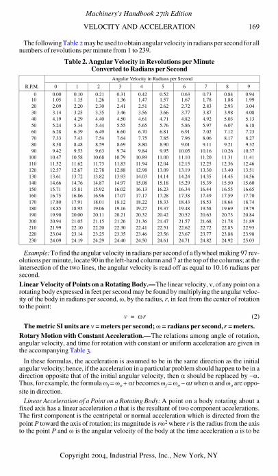
VELOCITY AND ACCELERATION 169
The following Table 2 may be used to obtain angular velocity in radians per second for allnumbers of revolutions per minute from 1 to 239.
Example:To find the angular velocity in radians per second of a flywheel making 97 rev-olutions per minute, locate 90 in the left-hand column and 7 at the top of the columns; at theintersection of the two lines, the angular velocity is read off as equal to 10.16 radians persecond.Linear Velocity of Points on a Rotating Body.—The linear velocity, ν, of any point on arotating body expressed in feet per second may be found by multiplying the angular veloc-ity of the body in radians per second, ω, by the radius, r, in feet from the center of rotationto the point:
(2)
The metric SI units are ν = meters per second; ω = radians per second, r = meters.Rotary Motion with Constant Acceleration.—The relations among angle of rotation,angular velocity, and time for rotation with constant or uniform acceleration are given inthe accompanying Table 3.
In these formulas, the acceleration is assumed to be in the same direction as the initialangular velocity; hence, if the acceleration in a particular problem should happen to be in adirection opposite that of the initial angular velocity, then α should be replaced by −α.Thus, for example, the formula ωf = ωo + αt becomes ωf = ωo − αt when α and ωo are oppo-site in direction.
Linear Acceleration of a Point on a Rotating Body: A point on a body rotating about afixed axis has a linear acceleration a that is the resultant of two component accelerations.The first component is the centripetal or normal acceleration which is directed from thepoint P toward the axis of rotation; its magnitude is rω2 where r is the radius from the axisto the point P and ω is the angular velocity of the body at the time acceleration a is to be
Table 2. Angular Velocity in Revolutions per Minute Converted to Radians per Second
R.P.M.
Angular Velocity in Radians per Second
0 1 2 3 4 5 6 7 8 9
0 0.00 0.10 0.21 0.31 0.42 0.52 0.63 0.73 0.84 0.9410 1.05 1.15 1.26 1.36 1.47 1.57 1.67 1.78 1.88 1.9920 2.09 2.20 2.30 2.41 2.51 2.62 2.72 2.83 2.93 3.0430 3.14 3.25 3.35 3.46 3.56 3.66 3.77 3.87 3.98 4.0840 4.19 4.29 4.40 4.50 4.61 4.71 4.82 4.92 5.03 5.1350 5.24 5.34 5.44 5.55 5.65 5.76 5.86 5.97 6.07 6.1860 6.28 6.39 6.49 6.60 6.70 6.81 6.91 7.02 7.12 7.2370 7.33 7.43 7.54 7.64 7.75 7.85 7.96 8.06 8.17 8.2780 8.38 8.48 8.59 8.69 8.80 8.90 9.01 9.11 9.21 9.3290 9.42 9.53 9.63 9.74 9.84 9.95 10.05 10.16 10.26 10.37
100 10.47 10.58 10.68 10.79 10.89 11.00 11.10 11.20 11.31 11.41110 11.52 11.62 11.73 11.83 11.94 12.04 12.15 12.25 12.36 12.46120 12.57 12.67 12.78 12.88 12.98 13.09 13.19 13.30 13.40 13.51130 13.61 13.72 13.82 13.93 14.03 14.14 14.24 14.35 14.45 14.56140 14.66 14.76 14.87 14.97 15.08 15.18 15.29 15.39 15.50 15.60150 15.71 15.81 15.92 16.02 16.13 16.23 16.34 16.44 16.55 16.65160 16.75 16.86 16.96 17.07 17.17 17.28 17.38 17.49 17.59 17.70170 17.80 17.91 18.01 18.12 18.22 18.33 18.43 18.53 18.64 18.74180 18.85 18.95 19.06 19.16 19.27 19.37 19.48 19.58 19.69 19.79190 19.90 20.00 20.11 20.21 20.32 20.42 20.52 20.63 20.73 20.84200 20.94 21.05 21.15 21.26 21.36 21.47 21.57 21.68 21.78 21.89210 21.99 22.10 22.20 22.30 22.41 22.51 22.62 22.72 22.83 22.93220 23.04 23.14 23.25 23.35 23.46 23.56 23.67 23.77 23.88 23.98230 24.09 24.19 24.29 24.40 24.50 24.61 24.71 24.82 24.92 25.03
v ωr=
Machinery's Handbook 27th Edition
Copyright 2004, Industrial Press, Inc., New York, NY
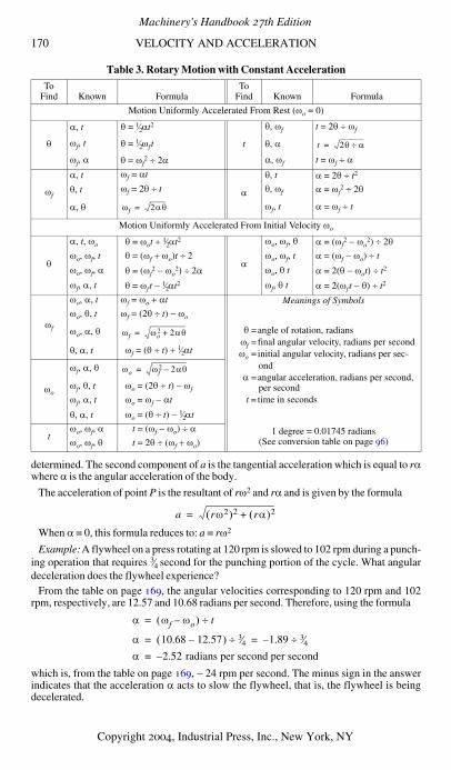
170 VELOCITY AND ACCELERATION
determined. The second component of a is the tangential acceleration which is equal to rαwhere α is the angular acceleration of the body.
The acceleration of point P is the resultant of rω2 and rα and is given by the formula
When α = 0, this formula reduces to: a = rω2
Example:A flywheel on a press rotating at 120 rpm is slowed to 102 rpm during a punch-ing operation that requires 3⁄4 second for the punching portion of the cycle. What angulardeceleration does the flywheel experience?
From the table on page 169, the angular velocities corresponding to 120 rpm and 102rpm, respectively, are 12.57 and 10.68 radians per second. Therefore, using the formula
which is, from the table on page 169, − 24 rpm per second. The minus sign in the answerindicates that the acceleration α acts to slow the flywheel, that is, the flywheel is beingdecelerated.
Table 3. Rotary Motion with Constant Acceleration
ToFind Known Formula
ToFind Known Formula
Motion Uniformly Accelerated From Rest (ωo = 0)
θ
α, t θ = 1⁄2αt2
t
θ, ωf t = 2θ ÷ ωf
ωf, t θ = 1⁄2ωf t θ, α
ωf, α θ = ωf2 ÷ 2α α, ωf t = ωf ÷ α
ωf
α, t ωf = αt
α
θ, t α = 2θ ÷ t2
θ, t ωf = 2θ ÷ t θ, ωf α = ωf2 ÷ 2θ
α, θ ωf, t α = ωf ÷ t
Motion Uniformly Accelerated From Initial Velocity ωo
θ
α, t, ωo θ = ωot + 1⁄2αt2
α
ωo, ωf, θ α = (ωf2 − ωo
2) ÷ 2θ
ωo, ωf, t θ = (ωf + ωo)t ÷ 2 ωo, ωf, t α = (ωf − ωo) ÷ t
ωo, ωf, α θ = (ωf2 − ωo
2) ÷ 2α ωo, θ t α = 2(θ − ωot) ÷ t2
ωf, α, t θ = ωf t − 1⁄2αt2 ωf, θ t α = 2(ωf t − θ) ÷ t2
ωf
ωo, α, t ωf = ωo + αt Meanings of Symbols
ωo, θ, t ωf = (2θ ÷ t) − ωo
θ =angle of rotation, radiansωf =final angular velocity, radians per secondωo =initial angular velocity, radians per sec-
ondα =angular acceleration, radians per second,
per secondt = time in seconds
ωo, α, θ
θ, α, t ωf = (θ ÷ t) + 1⁄2αt
ωo
ωf, α, θ
ωf, θ, t ωo = (2θ ÷ t) − ωf
ωf, α, t ωo = ωf − αt
θ, α, t ωo = (θ ÷ t) − 1⁄2αt
tωo, ωf, α t = (ωf − ωo) ÷ α 1 degree = 0.01745 radians
(See conversion table on page 96)ωo, ωf, θ t = 2θ ÷ (ωf + ωo)
t 2θ α÷=
ωf 2αθ=
ωf ωo2 2+ αθ=
ωo ωf2 2– αθ=
a rω2( )2 rα( )2+=
α ωf ωo–( ) t÷=
α 10.68 12.57–( ) 3⁄4÷ 1.89– 3⁄4÷= =
α 2.52– radians per second per second=
Machinery's Handbook 27th Edition
Copyright 2004, Industrial Press, Inc., New York, NY
FORCE 171
Force, Work, Energy, and Momentum
Accelerations Resulting from Unbalanced Forces.—In the section describing the reso-lution and composition of forces it was stated that when the resultant of a system of forcesis zero, the system is in equilibrium, that is, the body on which the force system actsremains at rest or continues to move with uniform velocity. If, however, the resultant of asystem of forces is not zero, the body on which the forces act will be accelerated in thedirection of the unbalanced force. To determine the relation between the unbalanced forceand the resulting acceleration, Newton's laws of motion must be applied. These laws maybe stated as follows:
First Law: Every body continues in a state of rest or in uniform motion in a straight line,until it is compelled by a force to change its state of rest or motion.
Second Law: Change of motion is proportional to the force applied, and takes place alongthe straight line in which the force acts. The “force applied” represents the resultant of allthe forces acting on the body. This law is sometimes worded: An unbalanced force actingon a body causes an acceleration of the body in the direction of the force and of magnitudeproportional to the force and inversely proportional to the mass of the body. Stated as a for-mula, R = Ma where R is the resultant of all the forces acting on the body, M is the mass ofthe body (mass = weight W divided by acceleration due to gravity g), and a is the accelera-tion of the body resulting from application of force R.
Third Law: To every action there is always an equal reaction, or, in other words, if a forceacts to change the state of motion of a body, the body offers a resistance equal and directlyopposite to the force.
Newton's second law may be used to calculate linear and angular accelerations of a bodyproduced by unbalanced forces and torques acting on the body; however, it is necessaryfirst to use the methods described under Algebraic Composition and Resolution of ForceSystems starting on page 148 to determine the magnitude and direction of the resultant ofall forces acting on the body. Then, for a body moving with pure translation,
where R is the resultant force in pounds acting on a body weighing W pounds; g is the grav-itational constant, usually taken as 32.16 ft/sec2, approximately; and a is the resultingacceleration in ft/sec2 of the body due to R and in the same direction as R.
Using metric SI units, the formula is R = Ma, where R = force in newtons (N), M =mass in kilograms, and a = acceleration in meters/second squared. It should be notedthat the weight of a body of mass M kg is Mg newtons, where g is approximately 9.81m/s2.
Free Body Diagram: In order to correctly determine the effect of forces on the motion ofa body it is necessary to resort to what is known as a free body diagram. Th i s d i ag ramshows 1) the body removed or isolated from contact with all other bodies that exert forceon the body and; and 2) all the forces acting on the body.
Thus, for example, in Fig. 1a the block being pulled up the plane is acted upon by certainforces; the free body diagram of this block is shown at Fig. 1b. Note that all forces acting onthe block are indicated. These forces include: 1) the force of gravity (weight); 2) the pullof the cable, P; 3) the normal component, W cos φ, of the force exerted on the block by theplane; and 4) the friction force, µW cos φ, of the plane on the block.
R Ma Wg-----a= =
Machinery's Handbook 27th Edition
Copyright 2004, Industrial Press, Inc., New York, NY
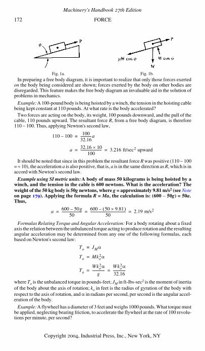
172 FORCE
In preparing a free body diagram, it is important to realize that only those forces exertedon the body being considered are shown; forces exerted by the body on other bodies aredisregarded. This feature makes the free body diagram an invaluable aid in the solution ofproblems in mechanics.
Example:A 100-pound body is being hoisted by a winch, the tension in the hoisting cablebeing kept constant at 110 pounds. At what rate is the body accelerated?
Two forces are acting on the body, its weight, 100 pounds downward, and the pull of thecable, 110 pounds upward. The resultant force R, from a free body diagram, is therefore110 − 100. Thus, applying Newton's second law,
It should be noted that since in this problem the resultant force R was positive (110 − 100= + 10), the acceleration a is also positive, that is, a is in the same direction as R, which is inaccord with Newton's second law.
Example using SI metric units:A body of mass 50 kilograms is being hoisted by awinch, and the tension in the cable is 600 newtons. What is the acceleration? Theweight of the 50 kg body is 50g newtons, where g = approximately 9.81 m/s2 (see Noteon page 179). Applying the formula R = Ma, the calculation is: (600 − 50g) = 50a.Thus,
Formulas Relating Torque and Angular Acceleration: For a body rotating about a fixedaxis the relation between the unbalanced torque acting to produce rotation and the resultingangular acceleration may be determined from any one of the following formulas, eachbased on Newton's second law:
where To is the unbalanced torque in pounds-feet; JM in ft-lbs-sec2 is the moment of inertiaof the body about the axis of rotation; ko in feet is the radius of gyration of the body withrespect to the axis of rotation, and α in radians per second, per second is the angular accel-eration of the body.
Example:A flywheel has a diameter of 3 feet and weighs 1000 pounds. What torque mustbe applied, neglecting bearing friction, to accelerate the flywheel at the rate of 100 revolu-tions per minute, per second?
Fig. 1a. Fig. 1b.
110 100– 10032.16-------------a=
a 32.16 10×100
------------------------- 3.216 ft/sec2 upward= =
a 600 50g–50
------------------------ 600 50 9.81×( )–50
------------------------------------------ 2.19 m/s2= = =
To JMα=
To Mko2α=
To
Wko2α
g---------------
Wko2α
32.16---------------= =
Machinery's Handbook 27th Edition
Copyright 2004, Industrial Press, Inc., New York, NY
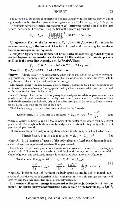
ENERGY 173
From page 250 the moment of inertia of a solid cylinder with respect to a gravity axis atright angles to the circular cross-section is given as 1⁄2 Mr2. From page 169, 100 rpm =10.47 radians per second, hence an acceleration of 100 rpm per second = 10.47 radians persecond, per second. Therefore, using the first of the preceding formulas,
Using metric SI units, the formulas are: To = JMα = Mko2α, where To = torque in
newton-meters; JM = the moment of inertia in kg · m2, and α = the angular accelera-tion in radians per second squared.
Example:A flywheel has a diameter of 1.5 m, and a mass of 800 kg. What torque isneeded to produce an angular acceleration of 100 revolutions per minute, per sec-ond? As in the preceding example, α = 10.47 rad/s2. Thus:
Therefore: To = JMα = 225 × 10.47 = 2356 N · m.
Energy.—A body is said to possess energy when it is capable of doing work or overcom-ing resistance. The energy may be either mechanical or non-mechanical, the latter includ-ing chemical, electrical, thermal, and atomic energy.
Mechanical energy includes kinetic energy (energy possessed by a body because of itsmotion) and potential energy (energy possessed by a body because of its position in a fieldof force and/or its elastic deformation).
Kinetic Energy: The motion of a body may be one of pure translation, pure rotation, or acombination of rotation and translation. By translation is meant motion in which every linein the body remains parallel to its original position throughout the motion, that is, no rota-tion is associated with the motion of the body.
The kinetic energy of a translating body is given by the formula
(3a)
where M = mass of body (= W ÷ g); V = velocity of the center of gravity of the body in feetper second; W = weight of body in pounds; and g = acceleration due to gravity = 32.16 feetper second, per second.
The kinetic energy of a body rotating about a fixed axis O is expressed by the formula:
(3b)
where JMO is the moment of inertia of the body about the fixed axis O in pounds-feet-seconds2, and ω = angular velocity in radians per second.
For a body that is moving with both translation and rotation, the total kinetic energy isgiven by the following formula as the sum of the kinetic energy due to translation of thecenter of gravity and the kinetic energy due to rotation about the center of gravity:
(3c)
where JMG is the moment of inertia of the body about its gravity axis in pounds-feet-seconds2, k is the radius of gyration in feet with respect to an axis through the center ofgravity, and the other quantities are as previously defined.
In the metric SI system, energy is expressed as the joule (J). One joule = 1 newton-meter. The kinetic energy of a translating body is given by the formula EKT = 1⁄2MV2,
To JMα 12---⎝ ⎠⎛ ⎞ 1000
32.16------------- 3
2---⎝ ⎠⎛ ⎞ 2
10.47× 366 ft-lbs= = =
JM1⁄2Mr2 1⁄2 800 0.752×× 225 kg m2⋅= = =
Kinetic Energy in ft-lbs due to translation EKT1⁄2MV2 WV2
2g-----------= = =
Kinetic Energy in ft-lbs due to rotation EKR1⁄2JMOω
2= =
Total Kinetic Energy in ft-lbs ET1⁄2= MV2 1⁄2JMGω
2+=
WV2
2g----------- 1⁄2JMGω
2+= WV2
2g----------- 1⁄2
Wk2ω2
g-----------------+ W
2g------ V2 k2ω2+( )= =
Machinery's Handbook 27th Edition
Copyright 2004, Industrial Press, Inc., New York, NY
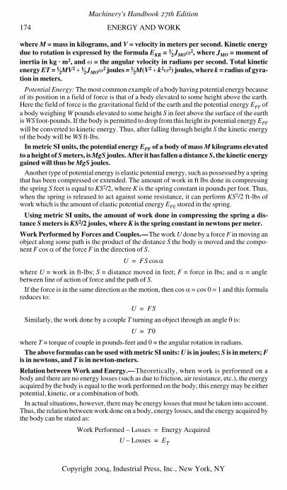
174 ENERGY AND WORK
where M = mass in kilograms, and V = velocity in meters per second. Kinetic energydue to rotation is expressed by the formula EKR = 1⁄2JMOω2, where JMO = moment ofinertia in kg · m2, and ω = the angular velocity in radians per second. Total kineticenergy ET = 1⁄2MV2 + 1⁄2JMOω2 joules = 1⁄2M(V2 + k2ω2) joules, where k = radius of gyra-tion in meters.
Potential Energy: The most common example of a body having potential energy becauseof its position in a field of force is that of a body elevated to some height above the earth.Here the field of force is the gravitational field of the earth and the potential energy EPF ofa body weighing W pounds elevated to some height S in feet above the surface of the earthis WS foot-pounds. If the body is permitted to drop from this height its potential energy EPF
will be converted to kinetic energy. Thus, after falling through height S the kinetic energyof the body will be WS ft-lbs.
In metric SI units, the potential energy EPF of a body of mass M kilograms elevatedto a height of S meters, is MgS joules. After it has fallen a distance S, the kinetic energygained will thus be MgS joules.
Another type of potential energy is elastic potential energy, such as possessed by a springthat has been compressed or extended. The amount of work in ft lbs done in compressingthe spring S feet is equal to KS2/2, where K is the spring constant in pounds per foot. Thus,when the spring is released to act against some resistance, it can perform KS2/2 ft-lbs ofwork which is the amount of elastic potential energy EPE stored in the spring.
Using metric SI units, the amount of work done in compressing the spring a dis-tance S meters is KS2/2 joules, where K is the spring constant in newtons per meter.
Work Performed by Forces and Couples.—The work U done by a force F in moving anobject along some path is the product of the distance S the body is moved and the compo-nent F cos α of the force F in the direction of S.
where U = work in ft-lbs; S = distance moved in feet; F = force in lbs; and α = anglebetween line of action of force and the path of S.
If the force is in the same direction as the motion, then cos α = cos 0 = 1 and this formulareduces to:
Similarly, the work done by a couple T turning an object through an angle θ is:
where T = torque of couple in pounds-feet and θ = the angular rotation in radians.
The above formulas can be used with metric SI units: U is in joules; S is in meters; Fis in newtons, and T is in newton-meters.
Relation between Work and Energy.—Theoretically, when work is performed on abody and there are no energy losses (such as due to friction, air resistance, etc.), the energyacquired by the body is equal to the work performed on the body; this energy may be eitherpotential, kinetic, or a combination of both.
In actual situations, however, there may be energy losses that must be taken into account.Thus, the relation between work done on a body, energy losses, and the energy acquired bythe body can be stated as:
U FS αcos=
U FS=
U Tθ=
Work Performed Losses– Energy Acquired=
U Losses– ET=
Machinery's Handbook 27th Edition
Copyright 2004, Industrial Press, Inc., New York, NY
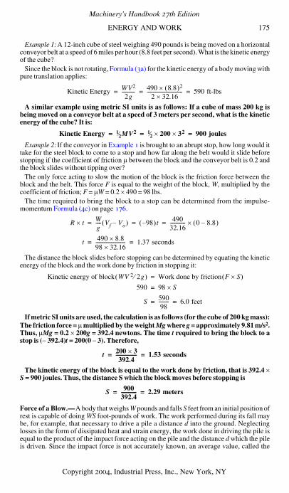
ENERGY AND WORK 175
Example 1:A 12-inch cube of steel weighing 490 pounds is being moved on a horizontalconveyor belt at a speed of 6 miles per hour (8.8 feet per second). What is the kinetic energyof the cube?
Since the block is not rotating, Formula (3a) for the kinetic energy of a body moving withpure translation applies:
A similar example using metric SI units is as follows: If a cube of mass 200 kg isbeing moved on a conveyor belt at a speed of 3 meters per second, what is the kineticenergy of the cube? It is:
Example 2:If the conveyor in Example 1 is brought to an abrupt stop, how long would ittake for the steel block to come to a stop and how far along the belt would it slide beforestopping if the coefficient of friction µ between the block and the conveyor belt is 0.2 andthe block slides without tipping over?
The only force acting to slow the motion of the block is the friction force between theblock and the belt. This force F is equal to the weight of the block, W, multiplied by thecoefficient of friction; F = µW = 0.2 × 490 = 98 lbs.
The time required to bring the block to a stop can be determined from the impulse-momentum Formula (4c) on page 176.
The distance the block slides before stopping can be determined by equating the kineticenergy of the block and the work done by friction in stopping it:
If metric SI units are used, the calculation is as follows (for the cube of 200 kg mass):The friction force = µ multiplied by the weight Mg where g = approximately 9.81 m/s2.Thus, µMg = 0.2 × 200g = 392.4 newtons. The time t required to bring the block to astop is (− 392.4)t = 200(0 − 3). Therefore,
The kinetic energy of the block is equal to the work done by friction, that is 392.4 ×S = 900 joules. Thus, the distance S which the block moves before stopping is
Force of a Blow.—A body that weighs W pounds and falls S feet from an initial position ofrest is capable of doing WS foot-pounds of work. The work performed during its fall maybe, for example, that necessary to drive a pile a distance d into the ground. Neglectinglosses in the form of dissipated heat and strain energy, the work done in driving the pile isequal to the product of the impact force acting on the pile and the distance d which the pileis driven. Since the impact force is not accurately known, an average value, called the
Kinetic Energy WV2
2g----------- 490 8.8( )2×
2 32.16×------------------------------ 590 ft-lbs= = =
Kinetic Energy 1⁄2MV2 1⁄2 200× 32× 900 joules= = =
R t× Wg----- Vf Vo–( ) 98–( )t 490
32.16------------- 0 8.8–( )×= = =
t 490 8.8×98 32.16×------------------------- 1.37 seconds= =
Kinetic energy of block WV 2 2g⁄( ) Work done by friction F S×( )=
590 98 S×=
S 59098--------- 6.0 feet= =
t 200 3×
392.4------------------ 1.53 seconds= =
S 900392.4------------- 2.29 meters= =
Machinery's Handbook 27th Edition
Copyright 2004, Industrial Press, Inc., New York, NY
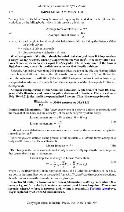
176 IMPULSE AND MOMENTUM
“average force of the blow,” may be assumed. Equating the work done on the pile and thework done by the falling body, which in this case is a pile driver:
where, S =total height in feet through which the driver falls, including the distance d thatthe pile is driven
W =weight of driver in poundsd =distance in feet which pile is driven
When using metric SI units, it should be noted that a body of mass M kilograms hasa weight of Mg newtons, where g = approximately 9.81 m/s2. If the body falls a dis-tance S meters, it can do work equal to MgS joules. The average force of the blow isMgS/d newtons, where d is the distance in meters that the pile is driven.
Example:A pile driver weighing 200 pounds strikes the top of the pile after having fallenfrom a height of 20 feet. It forces the pile into the ground a distance of 1⁄2 foot. Before theram is brought to rest, it will 200 × (20 + 1⁄2) = 4100 foot-pounds of work, and as this energyis expended in a distance of one-half foot, the average force of the blow equals 4100 ÷ 1⁄2 =8200 pounds.
A similar example using metric SI units is as follows: A pile driver of mass 100 kilo-grams falls 10 meters and moves the pile a distance of 0.3 meters. The work done =100g(10 + 0.3) joules, and it is expended in 0.3 meters. Thus, the average force is
Impulse and Momentum.—The linear momentum of a body is defined as the product ofthe mass M of the body and the velocity V of the center of gravity of the body:
(4a)
It should be noted that linear momentum is a vector quantity, the momentum being in thesame direction as V.
Linear impulse is defined as the product of the resultant R of all the forces acting on abody and the time t that the resultant acts:
(4b)
The change in the linear momentum of a body is numerically equal to the linear impulsethat causes the change in momentum:
(4c)
where V f, the final velocity of the body after time t, and V o, the initial velocity of the body,are both in the same direction as the applied force R. If Vo, and Vf are in opposite directions,then the minus sign in the formula becomes a plus sign.
In metric SI units, the formulas are: Linear Momentum = MV kg · m/s, where M =mass in kg, and V = velocity in meters per second; and Linear Impulse = Rt newton-seconds, where R = force in newtons, and t = time in seconds. In Formula (4c) above,W/g is replaced by M when SI units are used.
or,
Average force of blow d× WS=
Average force of blow WSd
--------=
100g 10.3×
0.3----------------------------- 33680 newtons or 33.68 kN=
Linear momentum MV or since M W g÷==
Linear momentum WVg
---------=
Linear Impulse Rt=
Linear Impulse change in Linear Momentum=
Rt Wg-----Vf
Wg-----Vo– W
g----- Vf Vo–( )= =
Machinery's Handbook 27th Edition
Copyright 2004, Industrial Press, Inc., New York, NY
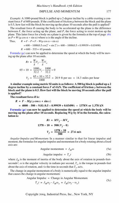
IMPULSE AND MOMENTUM 177
Example:A 1000-pound block is pulled up a 2-degree incline by a cable exerting a con-stant force F of 600 pounds. If the coefficient of friction µ between the block and the planeis 0.5, how fast will the block be moving up the plane 10 seconds after the pull is applied?
The resultant force R causing the body to be accelerated up the plane is the differencebetween F, the force acting up the plane, and P, the force acting to resist motion up theplane. This latter force for a body on a plane is given by the formula at the top of page 161as P = W (µ cos α + sin α) where α is the angle of the incline.
Formula (4c) can now be applied to determine the speed at which the body will be mov-ing up the plane after 10 seconds.
A similar example using metric SI units is as follows: A 500 kg block is pulled up a 2degree incline by a constant force F of 4 kN. The coefficient of friction µ between theblock and the plane is 0.5. How fast will the block be moving 10 seconds after the pullis applied?
The resultant force R is:
Formula (4c) can now be applied to determine the speed at which the body will bemoving up the plane after 10 seconds. Replacing W/g by M in the formula, the calcu-lation is:
Angular Impulse and Momentum: In a manner similar to that for linear impulse andmoment, the formulas for angular impulse and momentum for a body rotating about a fixedaxis are:
(5a)
(5b)
where JM is the moment of inertia of the body about the axis of rotation in pounds-feet-seconds2, ω is the angular velocity in radians per second, To, is the torque in pounds-feetabout the axis of rotation, and t is the time in seconds that To, acts.
The change in angular momentum of a body is numerically equal to the angular impulsethat causes the change in angular momentum:
(5c)
Thus, R = F − P = F − W(µ cos α + sin α)
= 600 − 1000(0.5 cos2° + sin 2°) = 600 − 1000(0.5 × 0.99939 + 0.03490)
R = 600 − 535 = 65 pounds.
Rt Wg-----Vf
Wg-----Vo–=
65 10× 100032.2------------Vf
100032.2------------ 0×–=
Vf65 10 32.2××
1000----------------------------------- 20.9 ft per sec 14.3 miles per hour= = =
R F Mg µ αcos αsin+( )–=
4000 500– 9.81 0.5 0.99939× 0.03490+( )×= 1378N or 1.378 kN=
Rt MVf MVo–=
1378 10× 500 Vf 0–( )=
Vf1378 10×
500------------------------ 27.6 m/s= =
Angular momentum JMω=
Angular impulse Tot=
Angular Impulse Change in Angular Momentum=
Tot JMωf JMωo– JM ωf ωo–( )= =
Machinery's Handbook 27th Edition
Copyright 2004, Industrial Press, Inc., New York, NY
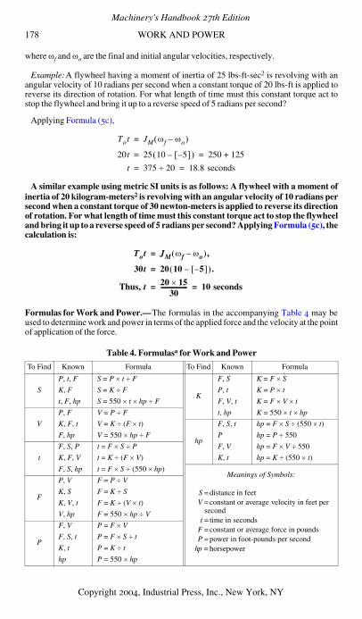
178 WORK AND POWER
where ωf and ωo are the final and initial angular velocities, respectively.
Example:A flywheel having a moment of inertia of 25 lbs-ft-sec2 is revolving with anangular velocity of 10 radians per second when a constant torque of 20 lbs-ft is applied toreverse its direction of rotation. For what length of time must this constant torque act tostop the flywheel and bring it up to a reverse speed of 5 radians per second?
Applying Formula (5c),
A similar example using metric SI units is as follows: A flywheel with a moment ofinertia of 20 kilogram-meters2 is revolving with an angular velocity of 10 radians persecond when a constant torque of 30 newton-meters is applied to reverse its directionof rotation. For what length of time must this constant torque act to stop the flywheeland bring it up to a reverse speed of 5 radians per second? Applying Formula (5c), thecalculation is:
Formulas for Work and Power.—The formulas in the accompanying Table 4 may beused to determine work and power in terms of the applied force and the velocity at the pointof application of the force.
Table 4. Formulasa for Work and Power
To Find Known Formula To Find Known Formula
S
P, t, F S = P × t ÷ F
K
F, S K = F × S
K, F S = K ÷ F P, t K = P × t
t, F, hp S = 550 × t × hp ÷ F F, V, t K = F × V × t
V
P, F V = P ÷ F t, hp K = 550 × t × hp
K, F, t V = K ÷ (F × t)
hp
F, S, t hp = F × S ÷ (550 × t)
F, hp V = 550 × hp ÷ F P hp = P ÷ 550
t
F, S, P t = F × S ÷ P F, V hp = F × V ÷ 550
K, F, V t = K ÷ (F × V) K, t hp = K ÷ (550 × t)
F, S, hp t = F × S ÷ (550 × hp)Meanings of Symbols:
F
P, V F = P ÷ V
K, S F = K ÷ S S =distance in feetV =constant or average velocity in feet per
secondt = time in seconds
F =constant or average force in poundsP =power in foot-pounds per second
hp = horsepower
K, V, t F = K ÷ (V × t)
V, hp F = 550 × hp ÷ V
P
F, V P = F × V
F, S, t P = F × S ÷ t
K, t P = K ÷ t
hp P = 550 × hp
Tot JM ωf ωo–( )=
20t 25 10 5–[ ]–( ) 250 125+= =
t 375 20÷ 18.8 seconds= =
Tot JM ωf ωo–( ) ,=
30t 20 10 5–[ ]–( ) .=
Thus, t 20 15×
30------------------ 10 seconds= =
Machinery's Handbook 27th Edition
Copyright 2004, Industrial Press, Inc., New York, NY
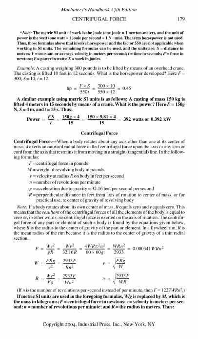
CENTRIFUGAL FORCE 179
Example:A casting weighing 300 pounds is to be lifted by means of an overhead crane.The casting is lifted 10 feet in 12 seconds. What is the horsepower developed? Here F =300; S = 10; t = 12.
A similar example using metric SI units is as follows: A casting of mass 150 kg islifted 4 meters in 15 seconds by means of a crane. What is the power? Here F = 150gN, S = 4 m, and t = 15 s. Thus:
Centrifugal Force
Centrifugal Force.—When a body rotates about any axis other than one at its center ofmass, it exerts an outward radial force called centrifugal force upon the axis or any arm orcord from the axis that restrains it from moving in a straight (tangential) line. In the follow-ing formulas:
F =centrifugal force in poundsW =weight of revolving body in poundsv =velocity at radius R on body in feet per secondn =number of revolutions per minuteg =acceleration due to gravity = 32.16 feet per second per secondR =perpendicular distance in feet from axis of rotation to center of mass, or for
practical use, to center of gravity of revolving body
Note: If a body rotates about its own center of mass, R equals zero and v equals zero. Thismeans that the resultant of the centrifugal forces of all the elements of the body is equal tozero or, in other words, no centrifugal force is exerted on the axis of rotation. The centrifu-gal force of any part or element of such a body is found by the equations given below,where R is the radius to the center of gravity of the part or element. In a flywheel rim, R isthe mean radius of the rim because it is the radius to the center of gravity of a thin radialsection.
(If n is the number of revolutions per second instead of per minute, then F = 1227WRn2.)If metric SI units are used in the foregoing formulas, W/g is replaced by M, which is
the mass in kilograms; F = centrifugal force in newtons; v = velocity in meters per sec-ond; n = number of revolutions per minute; and R = the radius in meters. Thus:
a Note: The metric SI unit of work is the joule (one joule = 1 newton-meter), and the unit ofpower is the watt (one watt = 1 joule per second = 1 N · m/s). The term horsepower is not used.Thus, those formulas above that involve horsepower and the factor 550 are not applicable whenworking in SI units. The remaining formulas can be used, and the units are: S = distance inmeters; V = constant or average velocity in meters per second; t = time in seconds; F = force innewtons; P = power in watts; K = work in joules.
hp F S×550t------------ 300 10×
550 12×--------------------- 0.45= = =
Power FSt
------- 150g 4×
15--------------------- 150 9.81× 4×
15----------------------------------- 392 watts or 0.392 kW= = = =
F Wv2
gR---------- Wv2
32.16R----------------- 4WRπ2n2
60 60g×------------------------- WRn2
2933--------------- 0.000341WRn2= = = = =
W FRgv2
----------- 2933FRn2
----------------= = v FRgW
-----------=
R Wv2
Fg---------- 2933F
Wn2----------------= = n 2933F
WR----------------=
Machinery's Handbook 27th Edition
Copyright 2004, Industrial Press, Inc., New York, NY
180 CENTRIFUGAL FORCE
If the rate of rotation is expressed as n1 = revolutions per second, then F = 39.48MRn1
2; if it is expressed as ω radians per second, then F = MRω2.
Calculating Centrifugal Force.—In the ordinary formula for centrifugal force, F =0.000341 WRn2; the mean radius R of the flywheel or pulley rim is given in feet. For smalldimensions, it is more convenient to have the formula in the form:
in which F = centrifugal force, in pounds; W = weight of rim, in pounds; r = mean radius ofrim, in inches; n = number of revolutions per minute.
In this formula let C = 0.000028416n2. This, then, is the centrifugal force of one pound,one inch from the axis. The formula can now be written in the form,
C is calculated for various values of the revolutions per minute n, and the calculated val-ues of C are given in Table 5. To find the centrifugal force in any given case, simply findthe value of C in the table and multiply it by the product of W and r, the four multiplicationsin the original formula given thus having been reduced to two.
Example:A cast-iron flywheel with a mean rim radius of 9 inches, is rotated at a speed of800 revolutions per minute. If the weight of the rim is 20 pounds, what is the centrifugalforce?
From Table 5, for n = 800 revolutions per minute, the value of C is 18.1862.Thus,
Using metric SI units, 0.01097n2 is the centrifugal force acting on a body of 1 kilo-gram mass rotating at n revolutions per minute at a distance of 1 meter from the axis.If this value is designated C1, then the centrifugal force of mass M kilograms rotatingat this speed at a distance from the axis of R meters, is C1MR newtons. To simplify cal-culations, values for C1 are given in Table 6. If it is required to work in terms of milli-meters, the force is 0.001 C1MR1 newtons, where R1 is the radius in millimeters.
Example:A steel pulley with a mean rim radius of 120 millimeters is rotated at aspeed of 1100 revolutions per minute. If the mass of the rim is 5 kilograms, what is thecentrifugal force?
From Table 6, for n = 1100 revolutions per minute, the value of C1 is 13,269.1.Thus,
Centrifugal Casting.—The centrifugal casting of metals is an old art. This process hasbecome important in such work as the manufacture of paper-mill rolls, railroad car wheels,and cast-iron pipe. The centrifugal casting process has been successfully applied in theproduction of non-metallic tubes, such as concrete pipe, in the production of solid castingsby locating the molds around the rim of a spinning wheel, and to a limited extent in the pro-duction of solid ingots by a largely similar process. Hollow objects such as cast-iron pipeare cast by introducing molten metal into a spinning mold. If the chilling of the metal isextremely rapid, for example in casting cast-iron pipe against a water-cooled chilled mold,it is imperative to use a movable spout. The particular feature that determines the field ofapplication of hot-mold centrifugal casting is the ability to produce long cast shapes ofcomparatively thin metal.
F Mv2 R⁄ Mn2 2πR2( )602R
------------------------------ 0.01097 MRn2= = =
F 0.2842-4×10 Wrn2=
F WrC=
F WrC 20 9× 18.1862× 3273.52 pounds= = =
F 0.001 C1MR1 0.001 13 269.1,× 5× 120× 7961.50 newtons = = =
Machinery's Handbook 27th Edition
Copyright 2004, Industrial Press, Inc., New York, NY
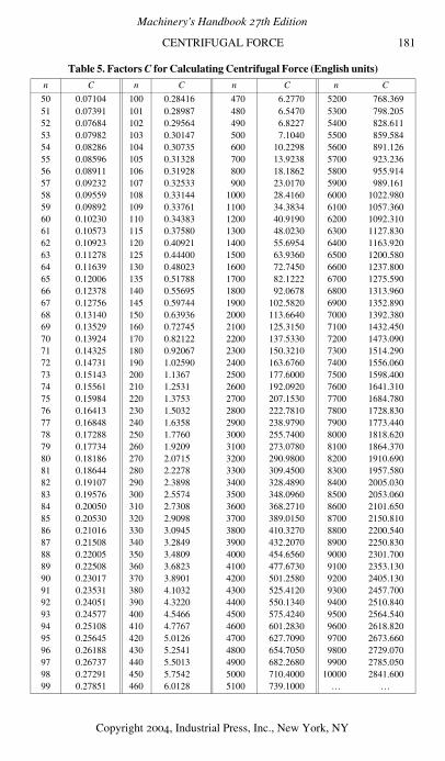
CENTRIFUGAL FORCE 181
Table 5. Factors C for Calculating Centrifugal Force (English units)
n C n C n C n C
50 0.07104 100 0.28416 470 6.2770 5200 768.36951 0.07391 101 0.28987 480 6.5470 5300 798.20552 0.07684 102 0.29564 490 6.8227 5400 828.61153 0.07982 103 0.30147 500 7.1040 5500 859.58454 0.08286 104 0.30735 600 10.2298 5600 891.12655 0.08596 105 0.31328 700 13.9238 5700 923.23656 0.08911 106 0.31928 800 18.1862 5800 955.91457 0.09232 107 0.32533 900 23.0170 5900 989.16158 0.09559 108 0.33144 1000 28.4160 6000 1022.98059 0.09892 109 0.33761 1100 34.3834 6100 1057.36060 0.10230 110 0.34383 1200 40.9190 6200 1092.31061 0.10573 115 0.37580 1300 48.0230 6300 1127.83062 0.10923 120 0.40921 1400 55.6954 6400 1163.92063 0.11278 125 0.44400 1500 63.9360 6500 1200.58064 0.11639 130 0.48023 1600 72.7450 6600 1237.80065 0.12006 135 0.51788 1700 82.1222 6700 1275.59066 0.12378 140 0.55695 1800 92.0678 6800 1313.96067 0.12756 145 0.59744 1900 102.5820 6900 1352.89068 0.13140 150 0.63936 2000 113.6640 7000 1392.38069 0.13529 160 0.72745 2100 125.3150 7100 1432.45070 0.13924 170 0.82122 2200 137.5330 7200 1473.09071 0.14325 180 0.92067 2300 150.3210 7300 1514.29072 0.14731 190 1.02590 2400 163.6760 7400 1556.06073 0.15143 200 1.1367 2500 177.6000 7500 1598.40074 0.15561 210 1.2531 2600 192.0920 7600 1641.31075 0.15984 220 1.3753 2700 207.1530 7700 1684.78076 0.16413 230 1.5032 2800 222.7810 7800 1728.83077 0.16848 240 1.6358 2900 238.9790 7900 1773.44078 0.17288 250 1.7760 3000 255.7400 8000 1818.62079 0.17734 260 1.9209 3100 273.0780 8100 1864.37080 0.18186 270 2.0715 3200 290.9800 8200 1910.69081 0.18644 280 2.2278 3300 309.4500 8300 1957.58082 0.19107 290 2.3898 3400 328.4890 8400 2005.03083 0.19576 300 2.5574 3500 348.0960 8500 2053.06084 0.20050 310 2.7308 3600 368.2710 8600 2101.65085 0.20530 320 2.9098 3700 389.0150 8700 2150.81086 0.21016 330 3.0945 3800 410.3270 8800 2200.54087 0.21508 340 3.2849 3900 432.2070 8900 2250.83088 0.22005 350 3.4809 4000 454.6560 9000 2301.70089 0.22508 360 3.6823 4100 477.6730 9100 2353.13090 0.23017 370 3.8901 4200 501.2580 9200 2405.13091 0.23531 380 4.1032 4300 525.4120 9300 2457.70092 0.24051 390 4.3220 4400 550.1340 9400 2510.84093 0.24577 400 4.5466 4500 575.4240 9500 2564.54094 0.25108 410 4.7767 4600 601.2830 9600 2618.82095 0.25645 420 5.0126 4700 627.7090 9700 2673.66096 0.26188 430 5.2541 4800 654.7050 9800 2729.07097 0.26737 440 5.5013 4900 682.2680 9900 2785.05098 0.27291 450 5.7542 5000 710.4000 10000 2841.60099 0.27851 460 6.0128 5100 739.1000 … …
Machinery's Handbook 27th Edition
Copyright 2004, Industrial Press, Inc., New York, NY
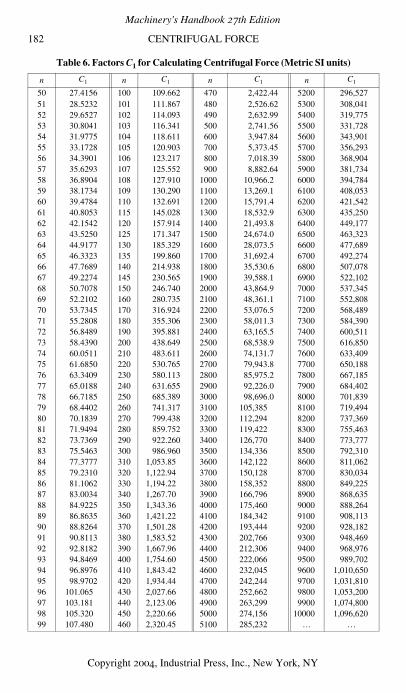
182 CENTRIFUGAL FORCE
Table 6. Factors C1 for Calculating Centrifugal Force (Metric SI units)
n C1 n C1 n C1 n C1
50 27.4156 100 109.662 470 2,422.44 5200 296,52751 28.5232 101 111.867 480 2,526.62 5300 308,04152 29.6527 102 114.093 490 2,632.99 5400 319,77553 30.8041 103 116.341 500 2,741.56 5500 331,72854 31.9775 104 118.611 600 3,947.84 5600 343,90155 33.1728 105 120.903 700 5,373.45 5700 356,29356 34.3901 106 123.217 800 7,018.39 5800 368,90457 35.6293 107 125.552 900 8,882.64 5900 381,73458 36.8904 108 127.910 1000 10,966.2 6000 394,78459 38.1734 109 130.290 1100 13,269.1 6100 408,05360 39.4784 110 132.691 1200 15,791.4 6200 421,54261 40.8053 115 145.028 1300 18,532.9 6300 435,25062 42.1542 120 157.914 1400 21,493.8 6400 449,17763 43.5250 125 171.347 1500 24,674.0 6500 463,32364 44.9177 130 185.329 1600 28,073.5 6600 477,68965 46.3323 135 199.860 1700 31,692.4 6700 492,27466 47.7689 140 214.938 1800 35,530.6 6800 507,07867 49.2274 145 230.565 1900 39,588.1 6900 522,10268 50.7078 150 246.740 2000 43,864.9 7000 537,34569 52.2102 160 280.735 2100 48,361.1 7100 552,80870 53.7345 170 316.924 2200 53,076.5 7200 568,48971 55.2808 180 355.306 2300 58,011.3 7300 584,39072 56.8489 190 395.881 2400 63,165.5 7400 600,51173 58.4390 200 438.649 2500 68,538.9 7500 616,85074 60.0511 210 483.611 2600 74,131.7 7600 633,40975 61.6850 220 530.765 2700 79,943.8 7700 650,18876 63.3409 230 580.113 2800 85,975.2 7800 667,18577 65.0188 240 631.655 2900 92,226.0 7900 684,40278 66.7185 250 685.389 3000 98,696.0 8000 701,83979 68.4402 260 741.317 3100 105,385 8100 719,49480 70.1839 270 799.438 3200 112,294 8200 737,36981 71.9494 280 859.752 3300 119,422 8300 755,46382 73.7369 290 922.260 3400 126,770 8400 773,77783 75.5463 300 986.960 3500 134,336 8500 792,31084 77.3777 310 1,053.85 3600 142,122 8600 811,06285 79.2310 320 1,122.94 3700 150,128 8700 830,03486 81.1062 330 1,194.22 3800 158,352 8800 849,22587 83.0034 340 1,267.70 3900 166,796 8900 868,63588 84.9225 350 1,343.36 4000 175,460 9000 888,26489 86.8635 360 1,421.22 4100 184,342 9100 908,11390 88.8264 370 1,501.28 4200 193,444 9200 928,18291 90.8113 380 1,583.52 4300 202,766 9300 948,46992 92.8182 390 1,667.96 4400 212,306 9400 968,97693 94.8469 400 1,754.60 4500 222,066 9500 989,70294 96.8976 410 1,843.42 4600 232,045 9600 1,010,65095 98.9702 420 1,934.44 4700 242,244 9700 1,031,81096 101.065 430 2,027.66 4800 252,662 9800 1,053,20097 103.181 440 2,123.06 4900 263,299 9900 1,074,80098 105.320 450 2,220.66 5000 274,156 10000 1,096,62099 107.480 460 2,320.45 5100 285,232 … …
Machinery's Handbook 27th Edition
Copyright 2004, Industrial Press, Inc., New York, NY
FLYWHEELS 183
FLYWHEELS
Classification of Flywheels
Flywheels may be classified as balance wheels or as flywheel pulleys. The object of allflywheels is to equalize the energy exerted and the work done and thereby prevent exces-sive or sudden changes of speed. The permissible speed variation is an important factor inall flywheel designs. The allowable speed change varies considerably for different classesof machinery; for instance, it is about 1 or 2 per cent in steam engines, while in punchingand shearing machinery a speed variation of 20 per cent may be allowed.
The function of a balance wheel is to absorb and equalize energy in case the resistance tomotion, or driving power, varies throughout the cycle. Therefore, the rim section is gener-ally quite heavy and is designed with reference to the energy that must be stored in it to pre-vent excessive speed variations and, with reference to the strength necessary to withstandsafely the stresses resulting from the required speed. The rims of most balance wheels areeither square or nearly square in section, but flywheel pulleys are commonly made wide toaccommodate a belt and relatively thin in a radial direction, although this is not an invari-able rule.
Flywheels, in general, may either be formed of a solid or one-piece section, or they maybe of sectional construction. Flywheels in diameters up to about eight feet are usually castsolid, the hubs sometimes being divided to relieve cooling stresses. Flywheels rangingfrom, say, eight feet to fifteen feet in diameter, are commonly cast in half sections, and thelarger sizes in several sections, the number of which may equal the number of arms in thewheel. Sectional flywheels may be divided into two general classes. One class includescast wheels which are formed of sections principally because a solid casting would be toolarge to transport readily. The second class includes wheels of sectional constructionwhich, by reason of the materials used and the special arrangement of the sections, enablesmuch higher peripheral speeds to be obtained safely than would be possible with ordinarysectional wheels of the type not designed especially for high speeds. Various designs havebeen built to withstand the extreme stresses encountered in some classes of service. Therims in some designs are laminated, being partly or entirely formed of numerous segment-shaped steel plates. Another type of flywheel, which is superior to an ordinary sectionalwheel, has a solid cast-iron rim connected to the hub by disk-shaped steel plates instead ofcast spokes.
Steel wheels may be divided into three distinct types, including 1) those having the cen-ter and rim built up entirely of steel plates; 2) those having a cast-iron center and steelrim; and 3) those having a cast-steel center and rim formed of steel plates.
Wheels having wire-wound rims have been used to a limited extent when extremely highspeeds have been necessary.
When the rim is formed of sections held together by joints it is very important to designthese joints properly. The ordinary bolted and flanged rim joints located between the armsaverage about 20 per cent of the strength of a solid rim and about 25 per cent is the maxi-mum strength obtainable for a joint of this kind. However, by placing the joints at the endsof the arms instead of between them, an efficiency of 50 per cent of the strength of the rimmay be obtained, because the joint is not subjected to the outward bending stressesbetween the arms but is directly supported by the arm, the end of which is secured to the rimjust beneath the joint. When the rim sections of heavy balance wheels are held together bysteel links shrunk into place, an efficiency of 60 per cent may be obtained; and by using arim of box or I-section, a link type of joint connection may have an efficiency of 100 per-cent.
Machinery's Handbook 27th Edition
Copyright 2004, Industrial Press, Inc., New York, NY

184 FLYWHEELS
Flywheel Calculations
Energy Due to Changes of Velocity.—When a flywheel absorbs energy from a variabledriving force, as in a steam engine, the velocity increases; and when this stored energy isgiven out, the velocity diminishes. When the driven member of a machine encounters avariable resistance in performing its work, as when the punch of a punching machine ispassing through a steel plate, the flywheel gives up energy while the punch is at work, and,consequently, the speed of the flywheel is reduced. The total energy that a flywheel wouldgive out if brought to a standstill is given by the formula:
in which E =total energy of flywheel, in foot-poundsW =weight of flywheel rim, in poundsv =velocity at mean radius of flywheel rim, in feet per secondg =acceleration due to gravity = 32.16 ft/s2
If the velocity of a flywheel changes, the energy it will absorb or give up is proportionalto the difference between the squares of its initial and final speeds, and is equal to the dif-ference between the energy that it would give out if brought to a full stop and the energythat is still stored in it at the reduced velocity. Hence:
in which E1 =energy in foot-pounds that a flywheel will give out while the speed isreduced from v1 to v2
W =weight of flywheel rim, in poundsv1 =velocity at mean radius of flywheel rim before any energy has been given
out, in feet per secondv2 =velocity of flywheel rim at end of period during which the energy has been
given out, in feet per secondOrdinarily, the effects of the arms and hub do not enter into flywheel calculations, and
only the weight of the rim is considered. In computing the velocity, the mean radius of therim is commonly used.
Using metric SI units, the formulas are E = 1⁄2Mv2, and E1 = 1⁄2M(v12 – v2
2), where Eand E1 are in joules; M = the mass of the rim in kilograms; and v, v1, and v2 = velocitiesin meters per second. Note: In the SI, the unit of mass is the kilogram. If the weight ofthe flywheel rim is given in kilograms, the value referred to is the mass, M. Should theweight be given in newtons, N, then
where g is approximately 9.81 meters per second squared.General Procedure in Flywheel Design.—The general method of designing a flywheelis to determine first the value of E1 or the energy the flywheel must either supply or absorbfor a given change in velocity, which, in turn, varies for different classes of service. Themean diameter of the flywheel may be assumed, or it may be fixed within certain limits bythe general design of the machine. Ordinarily the speed of the flywheel shaft is known, atleast approximately; the values of v1 and v2 can then be determined, the latter dependingupon the allowable percentage of speed variation. When these values are known, theweight of the rim and the cross-sectional area required to obtain this weight may be com-puted. The general procedure will be illustrated more in detail by considering the design offlywheels for punching and shearing machinery.
E Wv2
2g---------- Wv2
64.32-------------= =
E1
Wv12
2g----------
Wv22
2g----------–
W v12 v2
2–( )
64.32---------------------------= =
M W newtons( )g
-------------------------------=
Machinery's Handbook 27th Edition
Copyright 2004, Industrial Press, Inc., New York, NY
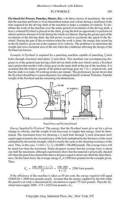
FLYWHEELS 185
Flywheels for Presses, Punches, Shears, Etc.—In these classes of machinery, the workthat the machine performs is of an intermittent nature and is done during a small part of thetime required for the driving shaft of the machine to make a complete revolution. To dis-tribute the work of the machine over the entire period of revolution of the driving shaft, aheavy-rimmed flywheel is placed on the shaft, giving the belt an opportunity to perform analmost uniform amount of work during the whole revolution. During the greater part of therevolution of the driving shaft, the belt power is used to accelerate the speed of the fly-wheel. During the part of the revolution when the work is done, the energy thus stored upin the flywheel is given out at the expense of its velocity. The problem is to determine theweight and cross-sectional area of the rim when the conditions affecting the design of theflywheel are known.
Example:A flywheel is required for a punching machine capable of punching 3⁄4-inchholes through structural steel plates 3⁄4 inch thick. This machine (see accompanying dia-gram) is of the general type having a belt-driven shaft at the rear which carries a flywheeland a pinion that meshes with a large gear on the main shaft at the top of the machine. It isassumed that the relative speeds of the pinion and large gear are 7 to 1, respectively, andthat the slide is to make 30 working strokes per minute. The preliminary layout shows thatthe flywheel should have a mean diameter (see enlarged detail) of about 30 inches. Find theweight of the flywheel and the remaining rim dimensions.
Punch Press and Flywheel Detail
Energy Supplied by Flywheel: The energy that the flywheel must give up for a givenchange in velocity, and the weight of rim necessary to supply that energy, must be deter-mined. The maximum force for shearing a 3⁄4-inch hole through 3⁄4-inch structural steelequals approximately the circumference of the hole multiplied by the thickness of the stockmultiplied by the tensile strength, which is nearly the same as the shearing resistance of thesteel. Thus, in this case, 3.1416 × 3⁄4 × 3⁄4 × 60,000 = 106,000 pounds. The average force willbe much less than the maximum. Some designers assume that the average force is aboutone-half the maximum, although experiments show that the material is practically shearedoff when the punch has entered the sheet a distance equal to about one-third the sheet thick-ness. On this latter basis, the average energy Ea is 2200 foot-pounds for the example given.Thus:
If the efficiency of the machine is taken as 85 per cent, the energy required will equal2200/0.85 = 2600 foot-pounds nearly. Assume that the energy supplied by the belt whilethe punch is at work is determined by calculation to equal 175 foot-pounds. Then the fly-wheel must supply 2600 −175 = 2425 foot-pounds = E1.
Ea106 000, 1⁄3× 3⁄4×
12----------------------------------------- 106 000,
4 12×--------------------- 2200 foot-pounds.= = =
Machinery's Handbook 27th Edition
Copyright 2004, Industrial Press, Inc., New York, NY
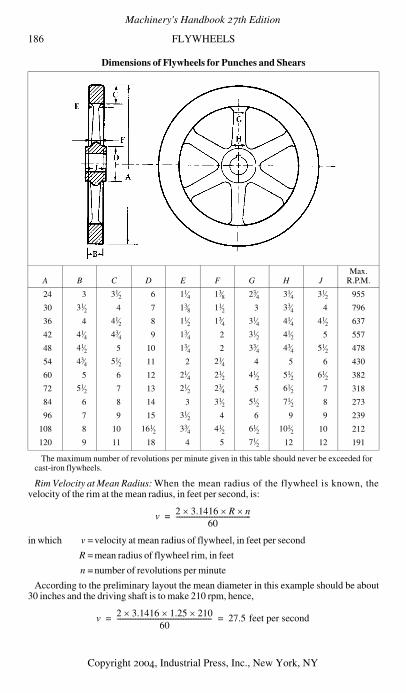
186 FLYWHEELS
Dimensions of Flywheels for Punches and Shears
The maximum number of revolutions per minute given in this table should never be exceeded forcast-iron flywheels.
Rim Velocity at Mean Radius: When the mean radius of the flywheel is known, thevelocity of the rim at the mean radius, in feet per second, is:
in which v =velocity at mean radius of flywheel, in feet per second
R =mean radius of flywheel rim, in feet
n =number of revolutions per minute
According to the preliminary layout the mean diameter in this example should be about30 inches and the driving shaft is to make 210 rpm, hence,
A B C D E F G H JMax.
R.P.M.
24 3 31⁄2 6 11⁄4 13⁄8 23⁄4 31⁄4 31⁄2 955
30 31⁄2 4 7 13⁄8 11⁄2 3 33⁄4 4 796
36 4 41⁄2 8 11⁄2 13⁄4 31⁄4 41⁄4 41⁄2 637
42 41⁄4 43⁄4 9 13⁄4 2 31⁄2 41⁄2 5 557
48 41⁄2 5 10 13⁄4 2 33⁄4 43⁄4 51⁄2 478
54 43⁄4 51⁄2 11 2 21⁄4 4 5 6 430
60 5 6 12 21⁄4 21⁄2 41⁄2 51⁄2 61⁄2 382
72 51⁄2 7 13 21⁄2 23⁄4 5 61⁄2 7 318
84 6 8 14 3 31⁄2 51⁄2 71⁄2 8 273
96 7 9 15 31⁄2 4 6 9 9 239
108 8 10 161⁄2 33⁄4 41⁄2 61⁄2 101⁄2 10 212
120 9 11 18 4 5 71⁄2 12 12 191
v 2 3.1416× R n××60
---------------------------------------------=
v 2 3.1416× 1.25× 210×60
--------------------------------------------------------- 27.5 feet per second= =
Machinery's Handbook 27th Edition
Copyright 2004, Industrial Press, Inc., New York, NY
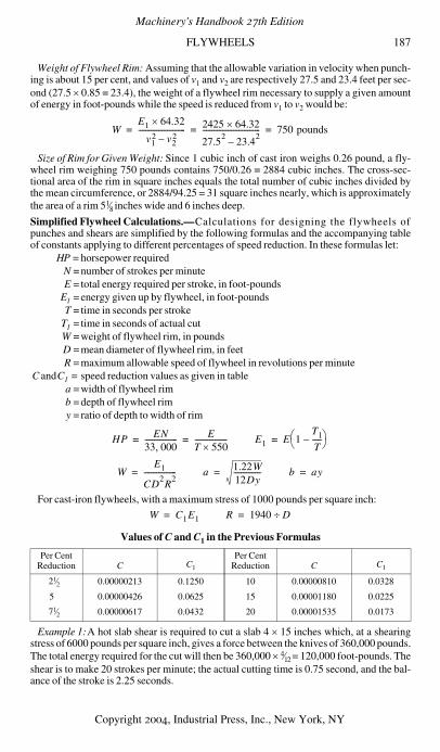
FLYWHEELS 187
Weight of Flywheel Rim: Assuming that the allowable variation in velocity when punch-ing is about 15 per cent, and values of v1 and v2 are respectively 27.5 and 23.4 feet per sec-ond (27.5 × 0.85 = 23.4), the weight of a flywheel rim necessary to supply a given amountof energy in foot-pounds while the speed is reduced from v1 to v2 would be:
Size of Rim for Given Weight: Since 1 cubic inch of cast iron weighs 0.26 pound, a fly-wheel rim weighing 750 pounds contains 750/0.26 = 2884 cubic inches. The cross-sec-tional area of the rim in square inches equals the total number of cubic inches divided bythe mean circumference, or 2884/94.25 = 31 square inches nearly, which is approximatelythe area of a rim 51⁄8 inches wide and 6 inches deep.
Simplified Flywheel Calculations.—Calculations for designing the flywheels ofpunches and shears are simplified by the following formulas and the accompanying tableof constants applying to different percentages of speed reduction. In these formulas let:
HP =horsepower requiredN =number of strokes per minuteE =total energy required per stroke, in foot-pounds
E1 =energy given up by flywheel, in foot-poundsT =time in seconds per stroke
T1 =time in seconds of actual cutW =weight of flywheel rim, in poundsD =mean diameter of flywheel rim, in feetR =maximum allowable speed of flywheel in revolutions per minute
C and C1 = speed reduction values as given in tablea =width of flywheel rimb =depth of flywheel rimy =ratio of depth to width of rim
For cast-iron flywheels, with a maximum stress of 1000 pounds per square inch:
Values of C and C1 in the Previous Formulas
Example 1:A hot slab shear is required to cut a slab 4 × 15 inches which, at a shearingstress of 6000 pounds per square inch, gives a force between the knives of 360,000 pounds.The total energy required for the cut will then be 360,000 × 4⁄12 = 120,000 foot-pounds. Theshear is to make 20 strokes per minute; the actual cutting time is 0.75 second, and the bal-ance of the stroke is 2.25 seconds.
Per CentReduction C C1
Per CentReduction C C1
21⁄2 0.00000213 0.1250 10 0.00000810 0.0328
5 0.00000426 0.0625 15 0.00001180 0.0225
71⁄2 0.00000617 0.0432 20 0.00001535 0.0173
WE1 64.32×
v12 v2
2–-------------------------- 2425 64.32×
27.52
23.42
–-------------------------------- 750 pounds= = =
HP EN33 000,------------------ E
T 550×------------------= = E1 E 1
T1
T-----–⎝ ⎠
⎛ ⎞=
WE1
CD2R
2------------------= a 1.22W
12Dy---------------= b ay=
W C1E1= R 1940 D÷=
Machinery's Handbook 27th Edition
Copyright 2004, Industrial Press, Inc., New York, NY
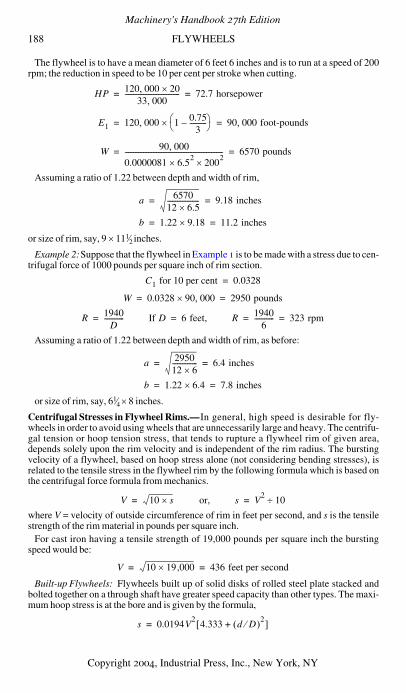
188 FLYWHEELS
The flywheel is to have a mean diameter of 6 feet 6 inches and is to run at a speed of 200rpm; the reduction in speed to be 10 per cent per stroke when cutting.
Assuming a ratio of 1.22 between depth and width of rim,
or size of rim, say, 9 × 111⁄2 inches.
Example 2:Suppose that the flywheel in Example 1 is to be made with a stress due to cen-trifugal force of 1000 pounds per square inch of rim section.
Assuming a ratio of 1.22 between depth and width of rim, as before:
or size of rim, say, 61⁄4 × 8 inches.
Centrifugal Stresses in Flywheel Rims.—In general, high speed is desirable for fly-wheels in order to avoid using wheels that are unnecessarily large and heavy. The centrifu-gal tension or hoop tension stress, that tends to rupture a flywheel rim of given area,depends solely upon the rim velocity and is independent of the rim radius. The burstingvelocity of a flywheel, based on hoop stress alone (not considering bending stresses), isrelated to the tensile stress in the flywheel rim by the following formula which is based onthe centrifugal force formula from mechanics.
where V = velocity of outside circumference of rim in feet per second, and s is the tensilestrength of the rim material in pounds per square inch.
For cast iron having a tensile strength of 19,000 pounds per square inch the burstingspeed would be:
Built-up Flywheels: Flywheels built up of solid disks of rolled steel plate stacked andbolted together on a through shaft have greater speed capacity than other types. The maxi-mum hoop stress is at the bore and is given by the formula,
HP 120 000, 20×33 000,
--------------------------------- 72.7 horsepower= =
E1 120 000, 1 0.753
----------–⎝ ⎠⎛ ⎞× 90 000 foot-pounds,= =
W 90 000,
0.0000081 6.52
× 2002
×----------------------------------------------------------- 6570 pounds= =
a 657012 6.5×------------------- 9.18 inches= =
b 1.22 9.18× 11.2 inches= =
C1 for 10 per cent 0.0328=
W 0.0328 90 000,× 2950 pounds= =
R 1940D
------------= If D 6 feet,= R 19406
------------ 323 rpm= =
a 295012 6×--------------- 6.4 inches= =
b 1.22 6.4× 7.8 inches= =
V 10 s× or,= s V2
10÷=
V 10 19 000,× 436 feet per second= =
s 0.0194V2
4.333 d D⁄( )2+[ ]=
Machinery's Handbook 27th Edition
Copyright 2004, Industrial Press, Inc., New York, NY
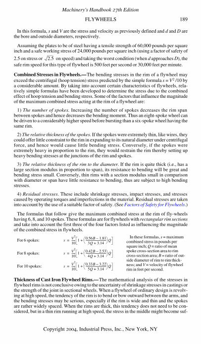
FLYWHEELS 189
In this formula, s and V are the stress and velocity as previously defined and d and D arethe bore and outside diameters, respectively.
Assuming the plates to be of steel having a tensile strength of 60,000 pounds per squareinch and a safe working stress of 24,000 pounds per square inch (using a factor of safety of
2.5 on stress or on speed) and taking the worst condition (when d approaches D), thesafe rim speed for this type of flywheel is 500 feet per second or 30,000 feet per minute.
Combined Stresses in Flywheels.—The bending stresses in the rim of a flywheel mayexceed the centrifugal (hoop tension) stress predicted by the simple formula s = V2 /10 bya considerable amount. By taking into account certain characteristics of flywheels, rela-tively simple formulas have been developed to determine the stress due to the combinedeffect of hoop tension and bending stress. Some of the factors that influence the magnitudeof the maximum combined stress acting at the rim of a flywheel are:
1) The number of spokes. Increasing the number of spokes decreases the rim spanbetween spokes and hence decreases the bending moment. Thus an eight-spoke wheel canbe driven to a considerably higher speed before bursting than a six-spoke wheel having thesame rim.
2) The relative thickness of the spokes. If the spokes were extremely thin, like wires, theycould offer little constraint to the rim in expanding to its natural diameter under centrifugalforce, and hence would cause little bending stress. Conversely, if the spokes wereextremely heavy in proportion to the rim, they would restrain the rim thereby setting upheavy bending stresses at the junctions of the rim and spokes.
3) The relative thickness of the rim to the diameter. If the rim is quite thick (i.e., has alarge section modulus in proportion to span), its resistance to bending will be great andbending stress small. Conversely, thin rims with a section modulus small in comparisonwith diameter or span have little resistance to bending, thus are subject to high bendingstresses.
4) Residual stresses. These include shrinkage stresses, impact stresses, and stressescaused by operating torques and imperfections in the material. Residual stresses are takeninto account by the use of a suitable factor of safety. (See Factors of Safety for Flywheels.)
The formulas that follow give the maximum combined stress at the rim of fly-wheelshaving 6, 8, and 10 spokes. These formulas are for flywheels with rectangular rim sectionsand take into account the first three of the four factors listed as influencing the magnitudeof the combined stress in flywheels.
Thickness of Cast Iron Flywheel Rims.—The mathematical analysis of the stresses inflywheel rims is not conclusive owing to the uncertainty of shrinkage stresses in castings orthe strength of the joint in sectional wheels. When a flywheel of ordinary design is revolv-ing at high speed, the tendency of the rim is to bend or bow outward between the arms, andthe bending stresses may be serious, especially if the rim is wide and thin and the spokesare rather widely spaced. When the rims are thick, this tendency does not need to be con-sidered, but in a thin rim running at high speed, the stress in the middle might become suf-
For 6 spokes:In these formulas, s = maximum
combined stress in pounds per square inch; Q = ratio of mean spoke cross-section area to rim cross-section area; B = ratio of out-side diameter of rim to rim thick-ness; and V = velocity of flywheel rim in feet per second.
For 8 spokes:
For 10 spokes:
2.5
s V2
10------ 1 0.56B 1.81–
3Q 3.14+-------------------------------⎝ ⎠⎛ ⎞Q+=
s V2
10------ 1 0.42B 2.53–
4Q 3.14+-------------------------------⎝ ⎠⎛ ⎞Q+=
s V2
10------ 1 0.33B 3.22–
5Q 3.14+-------------------------------⎝ ⎠⎛ ⎞Q+=
Machinery's Handbook 27th Edition
Copyright 2004, Industrial Press, Inc., New York, NY
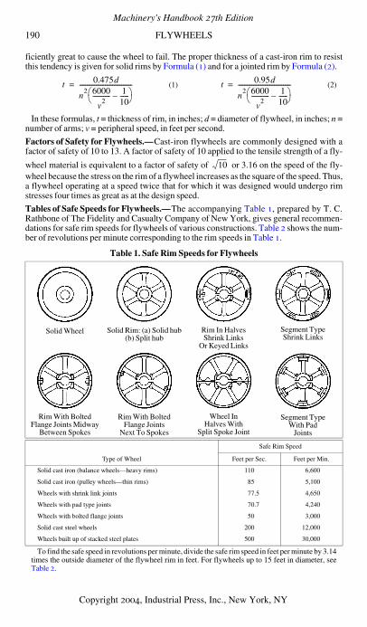
190 FLYWHEELS
ficiently great to cause the wheel to fail. The proper thickness of a cast-iron rim to resistthis tendency is given for solid rims by Formula (1) and for a jointed rim by Formula (2).
In these formulas, t = thickness of rim, in inches; d = diameter of flywheel, in inches; n =number of arms; v = peripheral speed, in feet per second.
Factors of Safety for Flywheels.—Cast-iron flywheels are commonly designed with afactor of safety of 10 to 13. A factor of safety of 10 applied to the tensile strength of a fly-
wheel material is equivalent to a factor of safety of or 3.16 on the speed of the fly-wheel because the stress on the rim of a flywheel increases as the square of the speed. Thus,a flywheel operating at a speed twice that for which it was designed would undergo rimstresses four times as great as at the design speed.
Tables of Safe Speeds for Flywheels.—The accompanying Table 1, prepared by T. C.Rathbone of The Fidelity and Casualty Company of New York, gives general recommen-dations for safe rim speeds for flywheels of various constructions. Table 2 shows the num-ber of revolutions per minute corresponding to the rim speeds in Table 1.
Table 1. Safe Rim Speeds for Flywheels
To find the safe speed in revolutions per minute, divide the safe rim speed in feet per minute by 3.14times the outside diameter of the flywheel rim in feet. For flywheels up to 15 feet in diameter, seeTable 2.
(1) (2)
Solid Wheel Solid Rim: (a) Solid hub(b) Split hub
Rim In HalvesShrink Links
Or Keyed Links
Segment TypeShrink Links
Rim With BoltedFlange Joints Midway
Between Spokes
Rim With BoltedFlange Joints
Next To Spokes
Wheel InHalves With
Split Spoke Joint
Segment TypeWith Pad
Joints
Type of Wheel
Safe Rim Speed
Feet per Sec. Feet per Min.
Solid cast iron (balance wheels—heavy rims) 110 6,600
Solid cast iron (pulley wheels—thin rims) 85 5,100
Wheels with shrink link joints 77.5 4,650
Wheels with pad type joints 70.7 4,240
Wheels with bolted flange joints 50 3,000
Solid cast steel wheels 200 12,000
Wheels built up of stacked steel plates 500 30,000
t 0.475d
n2 6000
v2
------------ 110------–⎝ ⎠
⎛ ⎞-----------------------------------= t 0.95d
n2 6000
v2
------------ 110------–⎝ ⎠
⎛ ⎞-----------------------------------=
10
Machinery's Handbook 27th Edition
Copyright 2004, Industrial Press, Inc., New York, NY
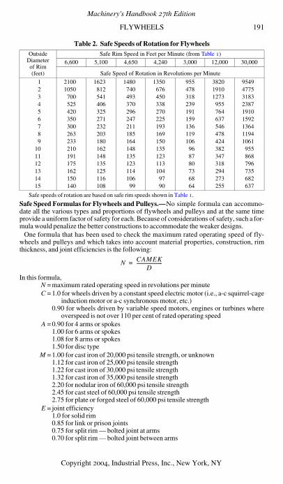
FLYWHEELS 191
Table 2. Safe Speeds of Rotation for Flywheels
Safe speeds of rotation are based on safe rim speeds shown in Table 1.
Safe Speed Formulas for Flywheels and Pulleys.—No simple formula can accommo-date all the various types and proportions of flywheels and pulleys and at the same timeprovide a uniform factor of safety for each. Because of considerations of safety, such a for-mula would penalize the better constructions to accommodate the weaker designs.
One formula that has been used to check the maximum rated operating speed of fly-wheels and pulleys and which takes into account material properties, construction, rimthickness, and joint efficiencies is the following:
In this formula, N =maximum rated operating speed in revolutions per minute
C =1.0 for wheels driven by a constant speed electric motor (i.e., a-c squirrel-cageinduction motor or a-c synchronous motor, etc.)
0.90 for wheels driven by variable speed motors, engines or turbines whereoverspeed is not over 110 per cent of rated operating speed
A =0.90 for 4 arms or spokes1.00 for 6 arms or spokes1.08 for 8 arms or spokes1.50 for disc type
M =1.00 for cast iron of 20,000 psi tensile strength, or unknown1.12 for cast iron of 25,000 psi tensile strength1.22 for cast iron of 30,000 psi tensile strength1.32 for cast iron of 35,000 psi tensile strength2.20 for nodular iron of 60,000 psi tensile strength2.45 for cast steel of 60,000 psi tensile strength2.75 for plate or forged steel of 60,000 psi tensile strength
E =joint efficiency1.0 for solid rim0.85 for link or prison joints0.75 for split rim — bolted joint at arms0.70 for split rim — bolted joint between arms
OutsideDiameterof Rim(feet)
Safe Rim Speed in Feet per Minute (from Table 1)6,600 5,100 4,650 4,240 3,000 12,000 30,000
Safe Speed of Rotation in Revolutions per Minute
1 2100 1623 1480 1350 955 3820 95492 1050 812 740 676 478 1910 47753 700 541 493 450 318 1273 31834 525 406 370 338 239 955 23875 420 325 296 270 191 764 19106 350 271 247 225 159 637 15927 300 232 211 193 136 546 13648 263 203 185 169 119 478 11949 233 180 164 150 106 424 1061
10 210 162 148 135 96 382 95511 191 148 135 123 87 347 86812 175 135 123 113 80 318 79613 162 125 114 104 73 294 73514 150 116 106 97 68 273 68215 140 108 99 90 64 255 637
N CAMEKD
----------------------=
Machinery's Handbook 27th Edition
Copyright 2004, Industrial Press, Inc., New York, NY

192 FLYWHEELS
K =1355 for rim thickness equal to 1 per cent of outside diameter1650 for rim thickness equal to 2 per cent of outside diameter1840 for rim thickness equal to 3 per cent of outside diameter1960 for rim thickness equal to 4 per cent of outside diameter2040 for rim thickness equal to 5 per cent of outside diameter2140 for rim thickness equal to 7 per cent of outside diameter2225 for rim thickness equal to 10 per cent of outside diameter2310 for rim thickness equal to 15 per cent of outside diameter2340 for rim thickness equal to 20 per cent of outside diameter
D =outside diameter of rim in feet
Example:A six-spoke solid cast iron balance wheel 8 feet in diameter has a rectangularrim 10 inches thick. What is the safe speed, in revolutions per minute, if driven by a con-stant speed motor?
In this instance, C = 1; A = 1; M = 1, since tensile strength is unknown; E = 1; K = 2225since the rim thickness is approximately 10 per cent of the wheel diameter; and D = 8 feet.Thus,
(Note: This safe speed is slightly greater than the value of 263 rpm obtainable directlyfrom Tables 1 and 2.)
Tests to Determine Flywheel Bursting Speeds.—Tests made by Prof. C. H. Benjamin,to determine the bursting speeds of flywheels, showed the following results:
Cast-iron Wheels with Solid Rims: Cast-iron wheels having solid rims burst at a rimspeed of 395 feet per second, corresponding to a centrifugal tension of about 15,600pounds per square inch.
Wheels with Jointed Rims: Four wheels were tested with joints and bolts inside the rim,using the familiar design ordinarily employed for band wheels, but with the joints locatedat points one-fourth of the distance from one arm to the next. These locations represent thepoints of least bending moment, and, consequently, the points at which the deflection dueto centrifugal force would be expected to have the least effect. The tests, however, did notbear out this conclusion. The wheels burst at a rim speed of 194 feet per second, corre-sponding to a centrifugal tension of about 3750 pounds per square inch. These wheels,therefore, were only about one-quarter as strong as the wheels with solid rims, and burst atpractically the same speed as wheels in a previous series of tests in which the rim jointswere midway between the arms.
Bursting Speed for Link Joints: Another type of wheel with deep rim, fastened togetherat the joints midway between the arms by links shrunk into recesses, after the manner offlywheels for massive engines, gave much superior results. This wheel burst at a speed of256 feet per second, indicating a centrifugal tension of about 6600 pounds per square inch.
Wheel having Tie-rods: Tests were made on a band wheel having joints inside the rim,midway between the arms, and in all respects like others of this design previously tested,except that tie-rods were used to connect the joints with the hub. This wheel burst at a speedof 225 feet per second, showing an increase of strength of from 30 to 40 per cent over sim-ilar wheels without the tie-rods.
Wheel Rim of I-section: Several wheels of special design, not in common use, were alsotested, the one giving the greatest strength being an English wheel, with solid rim of I-sec-tion, made of high-grade cast iron and with the rim tied to the hub by steel wire spokes.These spokes were adjusted to have a uniform tension. The wheel gave way at a rim speedof 424 feet per second, which is slightly higher than the speed of rupture of the solid rimwheels with ordinary style of spokes.
N 1 1× 1× 2225×8
--------------------------------------- 278 rpm= =
Machinery's Handbook 27th Edition
Copyright 2004, Industrial Press, Inc., New York, NY
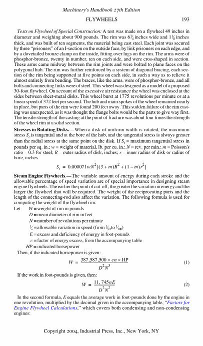
FLYWHEELS 193
Tests on Flywheel of Special Construction: A test was made on a flywheel 49 inches indiameter and weighing about 900 pounds. The rim was 63⁄4 inches wide and 11⁄8 inchesthick, and was built of ten segments, the material being cast steel. Each joint was securedby three “prisoners” of an I-section on the outside face, by link prisoners on each edge, andby a dovetailed bronze clamp on the inside, fitting over lugs on the rim. The arms were ofphosphor-bronze, twenty in number, ten on each side, and were cros-shaped in section.These arms came midway between the rim joints and were bolted to plane faces on thepolygonal hub. The rim was further reinforced by a system of diagonal bracing, each sec-tion of the rim being supported at five points on each side, in such a way as to relieve italmost entirely from bending. The braces, like the arms, were of phosphor-bronze, and allbolts and connecting links were of steel. This wheel was designed as a model of a proposed30-foot flywheel. On account of the excessive air resistance the wheel was enclosed at thesides between sheet-metal disks. This wheel burst at 1775 revolutions per minute or at alinear speed of 372 feet per second. The hub and main spokes of the wheel remained nearlyin place, but parts of the rim were found 200 feet away. This sudden failure of the rim cast-ing was unexpected, as it was thought the flange bolts would be the parts to give way first.The tensile strength of the casting at the point of fracture was about four times the strengthof the wheel rim at a solid section.Stresses in Rotating Disks.—When a disk of uniform width is rotated, the maximumstress St is tangential and at the bore of the hub, and the tangential stress is always greaterthan the radial stress at the same point on the disk. If St = maximum tangential stress inpounds per sq. in.; w = weight of material, lb. per cu. in.; N = rev. per min.; m = Poisson'sratio = 0.3 for steel; R = outer radius of disk, inches; r = inner radius of disk or radius ofbore, inches.
Steam Engine Flywheels.—The variable amount of energy during each stroke and theallowable percentage of speed variation are of special importance in designing steamengine flywheels. The earlier the point of cut-off, the greater the variation in energy and thelarger the flywheel that will be required. The weight of the reciprocating parts and thelength of the connecting-rod also affect the variation. The following formula is used forcomputing the weight of the flywheel rim:Let W =weight of rim in pounds
D =mean diameter of rim in feetN =number of revolutions per minute1⁄n =allowable variation in speed (from 1⁄50 to 1⁄100)E =excess and deficiency of energy in foot-poundsc =factor of energy excess, from the accompanying table
HP = indicated horsepowerThen, if the indicated horsepower is given:
(1)
If the work in foot-pounds is given, then:
(2)
In the second formula, E equals the average work in foot-pounds done by the engine inone revolution, multiplied by the decimal given in the accompanying table, “Factors forEngine Flywheel Calculations,” which covers both condensing and non-condensingengines:
St 0.000071wN2
3 m+( )R21 m–( )r2
+[ ]=
W 387 587 500,, cn× HP×
D2N
3---------------------------------------------------------=
W 11 745nE,
D2N
2-------------------------=
Machinery's Handbook 27th Edition
Copyright 2004, Industrial Press, Inc., New York, NY
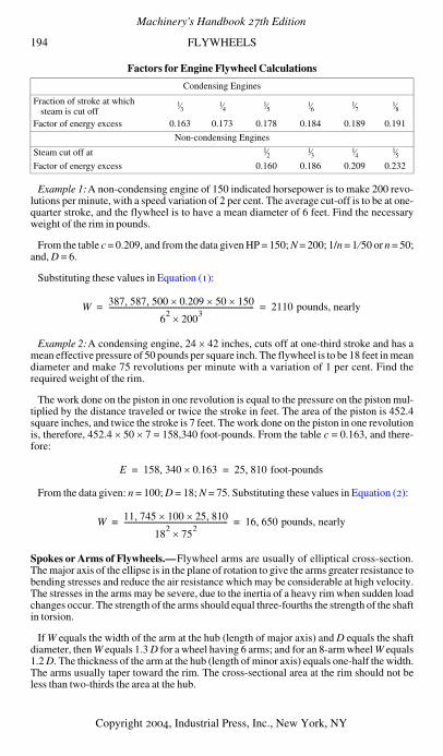
194 FLYWHEELS
Factors for Engine Flywheel Calculations
Example 1:A non-condensing engine of 150 indicated horsepower is to make 200 revo-lutions per minute, with a speed variation of 2 per cent. The average cut-off is to be at one-quarter stroke, and the flywheel is to have a mean diameter of 6 feet. Find the necessaryweight of the rim in pounds.
From the table c = 0.209, and from the data given HP = 150; N = 200; 1/n = 1 ⁄50 or n = 50;and, D = 6.
Substituting these values in Equation (1):
Example 2:A condensing engine, 24 × 42 inches, cuts off at one-third stroke and has amean effective pressure of 50 pounds per square inch. The flywheel is to be 18 feet in meandiameter and make 75 revolutions per minute with a variation of 1 per cent. Find therequired weight of the rim.
The work done on the piston in one revolution is equal to the pressure on the piston mul-tiplied by the distance traveled or twice the stroke in feet. The area of the piston is 452.4square inches, and twice the stroke is 7 feet. The work done on the piston in one revolutionis, therefore, 452.4 × 50 × 7 = 158,340 foot-pounds. From the table c = 0.163, and there-fore:
From the data given: n = 100; D = 18; N = 75. Substituting these values in Equation (2):
Spokes or Arms of Flywheels.—Flywheel arms are usually of elliptical cross-section.The major axis of the ellipse is in the plane of rotation to give the arms greater resistance tobending stresses and reduce the air resistance which may be considerable at high velocity.The stresses in the arms may be severe, due to the inertia of a heavy rim when sudden loadchanges occur. The strength of the arms should equal three-fourths the strength of the shaftin torsion.
If W equals the width of the arm at the hub (length of major axis) and D equals the shaftdiameter, then W equals 1.3 D for a wheel having 6 arms; and for an 8-arm wheel W equals1.2 D. The thickness of the arm at the hub (length of minor axis) equals one-half the width.The arms usually taper toward the rim. The cross-sectional area at the rim should not beless than two-thirds the area at the hub.
Condensing Engines
Fraction of stroke at which steam is cut off
1⁄31⁄4
1⁄51⁄6
1⁄71⁄8
Factor of energy excess 0.163 0.173 0.178 0.184 0.189 0.191
Non-condensing Engines
Steam cut off at 1⁄21⁄3
1⁄41⁄5
Factor of energy excess 0.160 0.186 0.209 0.232
W 387 587 500, , 0.209× 50× 150×
62
2003×
-------------------------------------------------------------------------------- 2110 pounds, nearly= =
E 158 340, 0.163× 25 810 foot-pounds,= =
W 11 745, 100× 25 810,×
182
752×
--------------------------------------------------------- 16 650 pounds, nearly,= =
Machinery's Handbook 27th Edition
Copyright 2004, Industrial Press, Inc., New York, NY
CRITICAL SPEEDS 195
Critical Speeds
Critical Speeds of Rotating Bodies and Shafts.—If a body or disk mounted upon a shaftrotates about it, the center of gravity of the body or disk must be at the center of the shaft, ifa perfect running balance is to be obtained. In most cases, however, the center of gravity ofthe disk will be slightly removed from the center of the shaft, owing to the difficulty of per-fect balancing. Now, if the shaft and disk be rotated, the centrifugal force generated by theheavier side will be greater than that generated by the lighter side geometrically opposite toit, and the shaft will deflect toward the heavier side, causing the center of the disk to rotatein a small circle. A rotating shaft without a body or disk mounted on it can also becomedynamically unstable, and the resulting vibrations and deflections can result in damage notonly to the shaft but to the machine of which it is a part. These conditions hold true up to acomparatively high speed; but a point is eventually reached (at several thousand revolu-tions per minute) when momentarily there will be excessive vibration, and then the partswill run quietly again. The speed at which this occurs is called the critical speed of thewheel or shaft, and the phenomenon itself for the shaft-mounted disk or body is called thesettling of the wheel. The explanation of the settling is that at this speed the axis of rotationchanges, and the wheel and shaft, instead of rotating about their geometrical center, beginto rotate about an axis through their center of gravity. The shaft itself is then deflected sothat for every revolution its geometrical center traces a circle around the center of gravityof the rotating mass.
Critical speeds depend upon the magnitude or location of the load or loads carried by theshaft, the length of the shaft, its diameter and the kind of supporting bearings. The normaloperating speed of a machine may or may not be higher than the critical speed. Forinstance, some steam turbines exceed the critical speed, although they do not run longenough at the critical speed for the vibrations to build up to an excessive amplitude. Thepractice of the General Electric Co. at Schenectady is to keep below the critical speeds. It isassumed that the maximum speed of a machine may be within 20 per cent high or low of thecritical speed without vibration troubles. Thus, in a design of steam turbine sets, criticalspeed is a factor that determines the size of the shafts for both the generators and turbines.Although a machine may run very close to the critical speed, the alignment and play of thebearings, the balance and construction generally, will require extra care, resulting in amore expensive machine; moreover, while such a machine may run smoothly for a consid-erable time, any looseness or play that may develop later, causing a slight imbalance, willimmediately set up excessive vibrations.
The formulas commonly used to determine critical speeds are sufficiently accurate forgeneral purposes. There are cases, however, where the torque applied to a shaft has animportant effect on its critical speed. Investigations have shown that the critical speeds ofa uniform shaft are decreased as the applied torque is increased, and that there exist criticaltorques which will reduce the corresponding critical speed of the shaft to zero. A detailedanalysis of the effects of applied torques on critical speeds may be found in a paper, “Crit-ical Speeds of Uniform Shafts under Axial Torque,” by Golumb and Rosenberg, presentedat the First U.S. National Congress of Applied Mechanics in 1951.Formulas for Critical Speeds.—The critical speed formulas given in the accompanyingtable (from the paper on Critical Speed Calculation presented before the ASME by S. H.Weaver) apply to (1) shafts with single concentrated loads and (2) shafts carrying uni-formly distributed loads. These formulas also cover different conditions as regards bear-ings. If the bearings are self-aligning or very short, the shaft is considered supported at theends; whereas, if the bearings are long and rigid, the shaft is considered fixed. These for-mulas, for both concentrated and distributed loads, apply to vertical shafts as well as hori-zontal shafts, the critical speeds having the same value in both cases. The data required forthe solution of critical speed problems are the same as for shaft deflection. As the shaft isusually of variable diameter and its stiffness is increased by a long hub, an ideal shaft ofuniform diameter and equal stiffness must be assumed.
Machinery's Handbook 27th Edition
Copyright 2004, Industrial Press, Inc., New York, NY
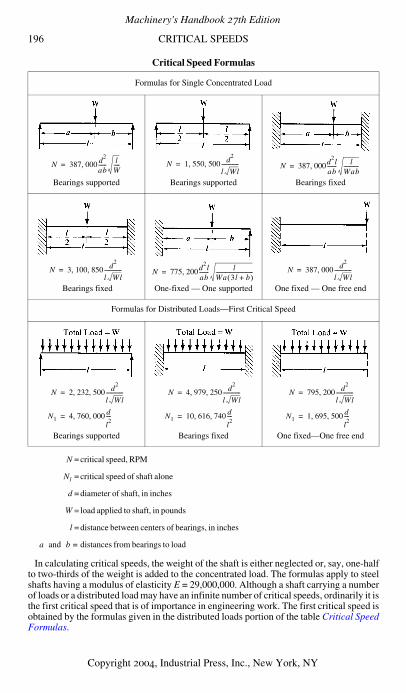
196 CRITICAL SPEEDS
Critical Speed Formulas
N =critical speed, RPM
N1 =critical speed of shaft alone
d =diameter of shaft, in inches
W = load applied to shaft, in pounds
l =distance between centers of bearings, in inches
a and b = distances from bearings to load
In calculating critical speeds, the weight of the shaft is either neglected or, say, one-halfto two-thirds of the weight is added to the concentrated load. The formulas apply to steelshafts having a modulus of elasticity E = 29,000,000. Although a shaft carrying a numberof loads or a distributed load may have an infinite number of critical speeds, ordinarily it isthe first critical speed that is of importance in engineering work. The first critical speed isobtained by the formulas given in the distributed loads portion of the table Critical SpeedFormulas.
Formulas for Single Concentrated Load
Bearings supported Bearings supported Bearings fixed
Bearings fixed One-fixed — One supported One fixed — One free end
Formulas for Distributed Loads—First Critical Speed
Bearings supported Bearings fixed One fixed—One free end
N 387 000 d2
ab------ l
W-----,= N 1 550 500 d
2
l Wl-------------, ,= N 387 000d
2l
ab------- l
Wab-----------,=
N 3 100 850 d2
l Wl-------------, ,= N 775 200d
2l
ab------- l
Wa 3l b+( )----------------------------,= N 387 000 d
2
l Wl-------------,=
N 2 232 500 d2
l Wl-------------, ,=
N1 4 760 000 d
l2
----, ,=
N 4 979 250 d2
l Wl-------------, ,=
N1 10 616 740 d
l2
----, ,=
N 795 200 d2
l Wl-------------,=
N1 1 695 500 d
l2
----, ,=
Machinery's Handbook 27th Edition
Copyright 2004, Industrial Press, Inc., New York, NY
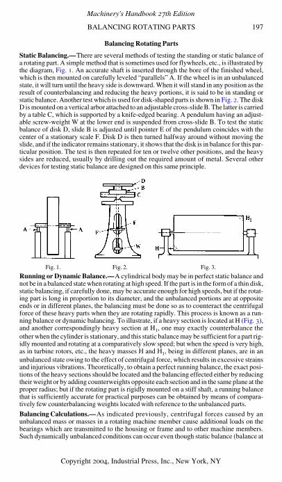
BALANCING ROTATING PARTS 197
Balancing Rotating Parts
Static Balancing.—There are several methods of testing the standing or static balance ofa rotating part. A simple method that is sometimes used for flywheels, etc., is illustrated bythe diagram, Fig. 1. An accurate shaft is inserted through the bore of the finished wheel,which is then mounted on carefully leveled “parallels” A. If the wheel is in an unbalancedstate, it will turn until the heavy side is downward. When it will stand in any position as theresult of counterbalancing and reducing the heavy portions, it is said to be in standing orstatic balance. Another test which is used for disk-shaped parts is shown in Fig. 2. The diskD is mounted on a vertical arbor attached to an adjustable cross-slide B. The latter is carriedby a table C, which is supported by a knife-edged bearing. A pendulum having an adjust-able screw-weight W at the lower end is suspended from cross-slide B. To test the staticbalance of disk D, slide B is adjusted until pointer E of the pendulum coincides with thecenter of a stationary scale F. Disk D is then turned halfway around without moving theslide, and if the indicator remains stationary, it shows that the disk is in balance for this par-ticular position. The test is then repeated for ten or twelve other positions, and the heavysides are reduced, usually by drilling out the required amount of metal. Several otherdevices for testing static balance are designed on this same principle.
Running or Dynamic Balance.—A cylindrical body may be in perfect static balance andnot be in a balanced state when rotating at high speed. If the part is in the form of a thin disk,static balancing, if carefully done, may be accurate enough for high speeds, but if the rotat-ing part is long in proportion to its diameter, and the unbalanced portions are at oppositeends or in different planes, the balancing must be done so as to counteract the centrifugalforce of these heavy parts when they are rotating rapidly. This process is known as a run-ning balance or dynamic balancing. To illustrate, if a heavy section is located at H (Fig. 3),and another correspondingly heavy section at H1, one may exactly counterbalance theother when the cylinder is stationary, and this static balance may be sufficient for a part rig-idly mounted and rotating at a comparatively slow speed; but when the speed is very high,as in turbine rotors, etc., the heavy masses H and H1, being in different planes, are in anunbalanced state owing to the effect of centrifugal force, which results in excessive strainsand injurious vibrations. Theoretically, to obtain a perfect running balance, the exact posi-tions of the heavy sections should be located and the balancing effected either by reducingtheir weight or by adding counterweights opposite each section and in the same plane at theproper radius; but if the rotating part is rigidly mounted on a stiff shaft, a running balancethat is sufficiently accurate for practical purposes can be obtained by means of compara-tively few counterbalancing weights located with reference to the unbalanced parts.
Balancing Calculations.—As indicated previously, centrifugal forces caused by anunbalanced mass or masses in a rotating machine member cause additional loads on thebearings which are transmitted to the housing or frame and to other machine members.Such dynamically unbalanced conditions can occur even though static balance (balance at
Fig. 1. Fig. 2. Fig. 3.
Machinery's Handbook 27th Edition
Copyright 2004, Industrial Press, Inc., New York, NY
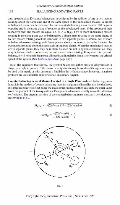
198 BALANCING ROTATING PARTS
zero speed) exists. Dynamic balance can be achieved by the addition of one or two massesrotating about the same axis and at the same speed as the unbalanced masses. A singleunbalanced mass can be balanced by one counterbalancing mass located 180 degreesopposite and in the same plane of rotation as the unbalanced mass, if the product of theirrespective radii and masses are equal; i.e., M1r1 = M2r2. Two or more unbalanced massesrotating in the same plane can be balanced by a single mass rotating in the same plane, orby two masses rotating about the same axis in two separate planes. Likewise, two or moreunbalanced masses rotating in different planes about a common axis can be balanced bytwo masses rotating about the same axis in separate planes. When the unbalanced massesare in separate planes they may be in static balance but not in dynamic balance; i.e., theymay be balanced when not rotating but unbalanced when rotating. If a system is in dynamicbalance, it will remain in balance at all speeds, although this is not strictly true at the criticalspeed of the system. (See Critical Speeds on page 195.)
In all the equations that follow, the symbol M denotes either mass in kilograms or inslugs, or weight in pounds. Either mass or weight units may be used and the equations maybe used with metric or with customary English units without change; however, in a givenproblem the units must be all metric or all customary English.
Counterbalancing Several Masses Located in a Single Plane.—In all balancing prob-lems, it is the product of counterbalancing mass (or weight) and its radius that is calculated;it is thus necessary to select either the mass or the radius and then calculate the other valuefrom the product of the two quantities. Design considerations usually make this decisionself-evident. The angular position of the counterbalancing mass must also be calculated.Referring to Fig. 4:
(1)
(2)
Fig. 4.
MBrB ΣMr θcos( )2 ΣMr θsin( )2+=
θtan BΣMr θsin( )–ΣMr θcos( )–
-------------------------------- yx--= =
Machinery's Handbook 27th Edition
Copyright 2004, Industrial Press, Inc., New York, NY
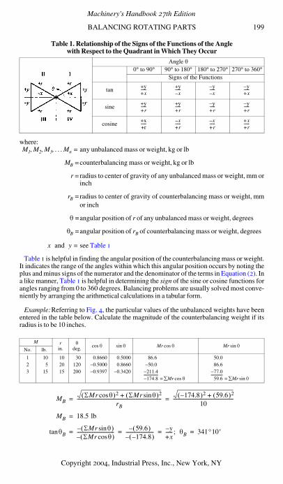
BALANCING ROTATING PARTS 199
Table 1. Relationship of the Signs of the Functions of the Angle with Respect to the Quadrant in Which They Occur
where: M1, M2, M3, . . . Mn = any unbalanced mass or weight, kg or lb
MB =counterbalancing mass or weight, kg or lb
r =radius to center of gravity of any unbalanced mass or weight, mm orinch
rB =radius to center of gravity of counterbalancing mass or weight, mmor inch
θ =angular position of r of any unbalanced mass or weight, degrees
θB =angular position of rB of counterbalancing mass or weight, degrees
x and y = see Table 1
Table 1 is helpful in finding the angular position of the counterbalancing mass or weight.It indicates the range of the angles within which this angular position occurs by noting theplus and minus signs of the numerator and the denominator of the terms in Equation (2). Ina like manner, Table 1 is helpful in determining the sign of the sine or cosine functions forangles ranging from 0 to 360 degrees. Balancing problems are usually solved most conve-niently by arranging the arithmetical calculations in a tabular form.
Example:Referring to Fig. 4, the particular values of the unbalanced weights have beenentered in the table below. Calculate the magnitude of the counterbalancing weight if itsradius is to be 10 inches.
Angle θ0° to 90° 90° to 180° 180° to 270° 270° to 360°
Signs of the Functions
tan
sine
cosine
M rin.
θ
deg. cos θ sin θ Mr cos θ Mr sin θNo. lb.
1 10 10 30 0.8660 0.5000 86.6 50.02 5 20 120 −0.5000 0.8660 −50.0 86.63 15 15 200 −0.9397 −0.3420 −211.4 −77.0
−174.8 = ∑Mr cos θ 59.6 = ∑Mr sin θ
+y+x------ +y
x–------ y–
x–------ y–
+x------
+y+r------ +y
+r------ y–
+r------ y–
+r------
+x+r------ x–
+r------ x–
+r------ +x
+r------
MBΣMr θcos( )2 ΣMr θsin( )2+
rB------------------------------------------------------------------------- 174.8–( )2 59.6( )2+
10----------------------------------------------------= =
MB 18.5 lb=
θBtan ΣMr θsin( )–ΣMr θcos( )–
-------------------------------- 59.6( )–174.8–( )–
------------------------ y–+x------ ; θB 341°10 ′= = = =
Machinery's Handbook 27th Edition
Copyright 2004, Industrial Press, Inc., New York, NY
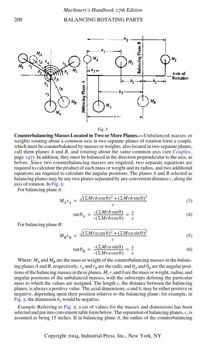
200 BALANCING ROTATING PARTS
Fig. 5.
Counterbalancing Masses Located in Two or More Planes.—Unbalanced masses orweights rotating about a common axis in two separate planes of rotation form a couple,which must be counterbalanced by masses or weights, also located in two separate planes,call them planes A and B, and rotating about the same common axis (see Couples,page 147). In addition, they must be balanced in the direction perpendicular to the axis, asbefore. Since two counterbalancing masses are required, two separate equations arerequired to calculate the product of each mass or weight and its radius, and two additionalequations are required to calculate the angular positions. The planes A and B selected asbalancing planes may be any two planes separated by any convenient distance c, along theaxis of rotation. In Fig. 5:
For balancing plane A:
(3)
(4)
For balancing plane B:
(5)
(6)
Where: MA and MB are the mass or weight of the counterbalancing masses in the balanc-ing planes A and B, respectively; rA and rB are the radii; and θA and θB are the angular posi-tions of the balancing masses in these planes. M, r, and θ are the mass or weight, radius, andangular positions of the unbalanced masses, with the subscripts defining the particularmass to which the values are assigned. The length c, the distance between the balancingplanes, is always a positive value. The axial dimensions, a and b, may be either positive ornegative, depending upon their position relative to the balancing plane; for example, inFig. 5, the dimension b2 would be negative.
Example:Referring to Fig. 5, a set of values for the masses and dimensions has beenselected and put into convenient table form below. The separation of balancing planes, c, isassumed as being 15 inches. If in balancing plane A, the radius of the counterbalancing
MArAΣMrb θcos( )2 ΣMrb θsin( )2+
c--------------------------------------------------------------------------------=
θAtan ΣMrb θsin( )–ΣMrb θcos( )–
------------------------------------ yx--= =
MBrBΣMra θcos( )2 ΣMra θsin( )2+
c--------------------------------------------------------------------------------=
θBtan ΣMra θsin( )–ΣMra θcos( )–
------------------------------------ yx--= =
Machinery's Handbook 27th Edition
Copyright 2004, Industrial Press, Inc., New York, NY
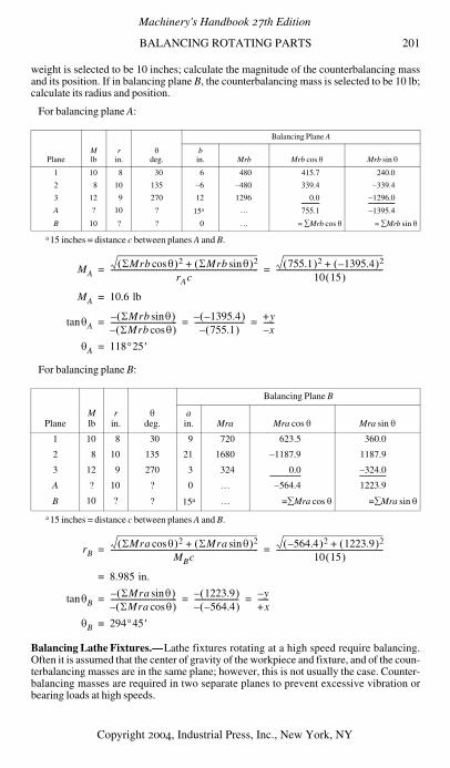
BALANCING ROTATING PARTS 201
weight is selected to be 10 inches; calculate the magnitude of the counterbalancing massand its position. If in balancing plane B, the counterbalancing mass is selected to be 10 lb;calculate its radius and position.
For balancing plane A:
For balancing plane B:
Balancing Lathe Fixtures.—Lathe fixtures rotating at a high speed require balancing.Often it is assumed that the center of gravity of the workpiece and fixture, and of the coun-terbalancing masses are in the same plane; however, this is not usually the case. Counter-balancing masses are required in two separate planes to prevent excessive vibration orbearing loads at high speeds.
PlaneMlb
rin.
θ
deg.
Balancing Plane A
bin. Mrb Mrb cos θ Mrb sin θ
1 10 8 30 6 480 415.7 240.0
2 8 10 135 −6 −480 339.4 −339.4
3 12 9 270 12 1296 0.0 −1296.0
A ? 10 ? 15a
a 15 inches = distance c between planes A and B.
… 755.1 −1395.4
B 10 ? ? 0 … = ∑Mrb cos θ = ∑Mrb sin θ
PlaneMlb
rin.
θ
deg.
Balancing Plane B
ain. Mra Mra cos θ Mra sin θ
1 10 8 30 9 720 623.5 360.0
2 8 10 135 21 1680 −1187.9 1187.9
3 12 9 270 3 324 0.0 −324.0
A ? 10 ? 0 … −564.4 1223.9
B 10 ? ? 15a
a 15 inches = distance c between planes A and B.
… =∑Mra cos θ =∑Mra sin θ
MAΣMrb θcos( )2 ΣMrb θsin( )2+
rAc-------------------------------------------------------------------------------- 755.1( )2 1395.4–( )2+
10 15( )----------------------------------------------------------= =
MA 10.6 lb=
θAtan ΣMrb θsin( )–ΣMrb θcos( )–
------------------------------------ 1395.4–( )–755.1( )–
--------------------------- +yx–
------= = =
θA 118°25 ′=
rBΣMra θcos( )2 ΣMra θsin( )2+
MBc-------------------------------------------------------------------------------- 564.4–( )2 1223.9( )2+
10 15( )----------------------------------------------------------= =
8.985 in.=
θBtan ΣMra θsin( )–ΣMra θcos( )–
------------------------------------ 1223.9( )–564.4–( )–
------------------------ y–+x------= = =
θB 294°45 ′=
Machinery's Handbook 27th Edition
Copyright 2004, Industrial Press, Inc., New York, NY
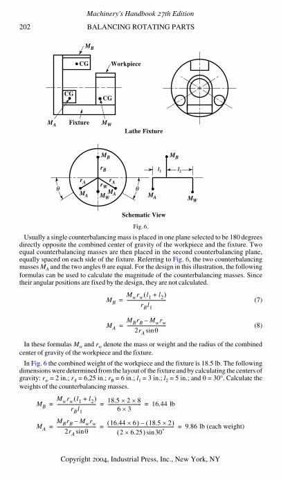
202 BALANCING ROTATING PARTS
Fig. 6.
Usually a single counterbalancing mass is placed in one plane selected to be 180 degreesdirectly opposite the combined center of gravity of the workpiece and the fixture. Twoequal counterbalancing masses are then placed in the second counterbalancing plane,equally spaced on each side of the fixture. Referring to Fig. 6, the two counterbalancingmasses MA and the two angles θ are equal. For the design in this illustration, the followingformulas can be used to calculate the magnitude of the counterbalancing masses. Sincetheir angular positions are fixed by the design, they are not calculated.
(7)
(8)
In these formulas Mw and rw denote the mass or weight and the radius of the combinedcenter of gravity of the workpiece and the fixture.
In Fig. 6 the combined weight of the workpiece and the fixture is 18.5 lb. The followingdimensions were determined from the layout of the fixture and by calculating the centers ofgravity: rw = 2 in.; rA = 6.25 in.; rB = 6 in.; l1 = 3 in.; l2 = 5 in.; and θ = 30°. Calculate theweights of the counterbalancing masses.
l2l1
CG
MA
MB MB
rB
rWrArA
MA MAMA
MB
MWFixture
CG
WorkpieceCG
Schematic View
Lathe Fixture
θ θMW MW
MB
Mwrw l1 l2+( )
rBl1----------------------------------=
MA
MBrB Mwrw–
2rA θsin----------------------------------=
MB
Mwrw l1 l2+( )
rBl1---------------------------------- 18.5 2× 8×
6 3×----------------------------- 16.44 lb= = =
MA
MBrB Mwrw–
2rA θsin---------------------------------- 16.44 6×( ) 18.5 2×( )–
2 6.25×( ) 30°sin---------------------------------------------------------- 9.86 lb (each weight)= = =
Machinery's Handbook 27th Edition
Copyright 2004, Industrial Press, Inc., New York, NY
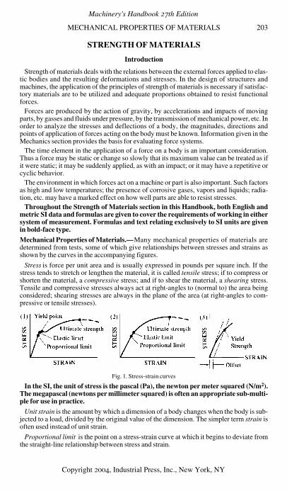
MECHANICAL PROPERTIES OF MATERIALS 203
STRENGTH OF MATERIALS
Introduction
Strength of materials deals with the relations between the external forces applied to elas-tic bodies and the resulting deformations and stresses. In the design of structures andmachines, the application of the principles of strength of materials is necessary if satisfac-tory materials are to be utilized and adequate proportions obtained to resist functionalforces.
Forces are produced by the action of gravity, by accelerations and impacts of movingparts, by gasses and fluids under pressure, by the transmission of mechanical power, etc. Inorder to analyze the stresses and deflections of a body, the magnitudes, directions andpoints of application of forces acting on the body must be known. Information given in theMechanics section provides the basis for evaluating force systems.
The time element in the application of a force on a body is an important consideration.Thus a force may be static or change so slowly that its maximum value can be treated as ifit were static; it may be suddenly applied, as with an impact; or it may have a repetitive orcyclic behavior.
The environment in which forces act on a machine or part is also important. Such factorsas high and low temperatures; the presence of corrosive gases, vapors and liquids; radia-tion, etc. may have a marked effect on how well parts are able to resist stresses.
Throughout the Strength of Materials section in this Handbook, both English andmetric SI data and formulas are given to cover the requirements of working in eithersystem of measurement. Formulas and text relating exclusively to SI units are givenin bold-face type.
Mechanical Properties of Materials.—Many mechanical properties of materials aredetermined from tests, some of which give relationships between stresses and strains asshown by the curves in the accompanying figures.
Stress is force per unit area and is usually expressed in pounds per square inch. If thestress tends to stretch or lengthen the material, it is called tensile stress; if to compress orshorten the material, a compressive stress; and if to shear the material, a shearing stress.Tensile and compressive stresses always act at right-angles to (normal to) the area beingconsidered; shearing stresses are always in the plane of the area (at right-angles to com-pressive or tensile stresses).
Fig. 1. Stress-strain curves
In the SI, the unit of stress is the pascal (Pa), the newton per meter squared (N/m2).The megapascal (newtons per millimeter squared) is often an appropriate sub-multi-ple for use in practice.
Unit strain is the amount by which a dimension of a body changes when the body is sub-jected to a load, divided by the original value of the dimension. The simpler term strain isoften used instead of unit strain.
Proportional limit is the point on a stress-strain curve at which it begins to deviate fromthe straight-line relationship between stress and strain.
Machinery's Handbook 27th Edition
Copyright 2004, Industrial Press, Inc., New York, NY

204 MECHANICAL PROPERTIES OF MATERIALS
Elastic limit is the maximum stress to which a test specimen may be subjected and stillreturn to its original length upon release of the load. A material is said to be stressed withinthe elastic region when the working stress does not exceed the elastic limit, and to bestressed in the plastic region when the working stress does exceed the elastic limit. Theelastic limit for steel is for all practical purposes the same as its proportional limit.
Yield point is a point on the stress-strain curve at which there is a sudden increase in strainwithout a corresponding increase in stress. Not all materials have a yield point. Some rep-resentative values of the yield point (in ksi) are as follows:
Yield strength, Sy, is the maximum stress that can be applied without permanent deforma-tion of the test specimen. This is the value of the stress at the elastic limit for materials forwhich there is an elastic limit. Because of the difficulty in determining the elastic limit, andbecause many materials do not have an elastic region, yield strength is often determined bythe offset method as illustrated by the accompanying figure at (3). Yield strength in such acase is the stress value on the stress-strain curve corresponding to a definite amount of per-manent set or strain, usually 0.1 or 0.2 per cent of the original dimension. Yield strengthdata for various materials are given in tables starting on pages 417, 419, 463, 464, 466,468, 472, 554, 556, 560, 569, 570, 575, 580, 588, 590, 591, and elsewhere.
Ultimate strength, Su, (also called tensile strength) is the maximum stress value obtainedon a stress-strain curve.
Modulus of elasticity, E, (also called Young's modulus) is the ratio of unit stress to unitstrain within the proportional limit of a material in tension or compression. Some represen-tative values of Young's modulus (in 106 psi) are as follows:
Modulus of elasticity in shear, G, is the ratio of unit stress to unit strain within the propor-tional limit of a material in shear.
Poisson's ratio, µ, is the ratio of lateral strain to longitudinal strain for a given materialsubjected to uniform longitudinal stresses within the proportional limit. The term is foundin certain equations associated with strength of materials. Values of Poisson's ratio forcommon materials are as follows:
Aluminum, wrought, 2014-T6 60 Titanium, pure 55–70Aluminum, wrought, 6061-T6 35 Titanium, alloy, 5Al, 2.5Sn 110Beryllium copper 140 Steel for bridges and buildings,
ASTM A7-61T, all shapes33
Brass, naval 25–50Cast iron, malleable 32–45 Steel, castings, high strength, for structural pur-
poses, ASTM A148.60 (seven grades)40–145
Cast iron, nodular 45–65Magnesium, AZ80A-T5 38 Steel, stainless (0.08–0.2C, 17Cr, 7Ni) 1⁄4 hard 78
Aluminum, cast, pure 9 Magnesium, AZ80A-T5 6.5Aluminum, wrought, 2014-T6 10.6 Titanium, pure 15.5Beryllium copper 19 Titanium, alloy, 5 Al, 2.5 Sn 17Brass, naval 15 Steel for bridges and buildings,
ASTM A7-61T, all shapes29
Bronze, phosphor, ASTM B159 15Cast iron, malleable 26 Steel, castings, high strength, for structural
purposes, ASTM A148-60 (seven grades)29
Cast iron, nodular 23.5
Aluminum 0.334 Nickel silver 0.322Beryllium copper 0.285 Phosphor bronze 0.349Brass 0.340 Rubber 0.500Cast iron, gray 0.211 Steel, cast 0.265Copper 0.340 high carbon 0.295Inconel 0.290 mild 0.303Lead 0.431 nickel 0.291Magnesium 0.350 Wrought iron 0.278Monel metal 0.320 Zinc 0.331
Machinery's Handbook 27th Edition
Copyright 2004, Industrial Press, Inc., New York, NY
SHEAR 205
Compressive Properties.—From compression tests, compressive yield strength, Scy, andcompressive ultimate strength, Scu, are determined. Ductile materials under compressionloading merely swell or buckle without fracture, hence do not have a compressive ultimatestrength.
Shear Properties.—The properties of shear yield strength, Ssy, shear ultimate strength,Ssu, and the modulus of rigidity, G, are determined by direct shear and torsional tests. Themodulus of rigidity is also known as the modulus of elasticity in shear. It is the ratio of theshear stress, τ, to the shear strain, γ, in radians, within the proportional limit: G = τ/γ.
Creep.—Continuing changes in dimensions of a stressed material over time is calledcreep, and it varies with different materials and periods under stress, also with temperature.Creep tests may take some time as it is necessary to apply a constant tensile load to a spec-imen under a selected temperature. Measurements are taken to record the resulting elonga-tion at time periods sufficiently long for a relationship to be established. The data are thenplotted as elongation against time. The load is applied to the specimen only after it hasreached the testing temperature, and causes an initial elastic elongation that includes someplastic deformation if the load is above the proportional limit for the material.
Some combinations of stress and temperature may cause failure of the specimen. Othersshow initial high rates of deformation, followed by decreasing, then constant, rates overlong periods. Generally testing times to arrive at the constant rate of deformation are over1000 hours.
Creep Rupture.—Tests for creep rupture are similar to creep tests but are prolonged untilthe specimen fails. Further data to be obtained from these tests include time to rupture,amount of elongation, and reduction of area. Stress-rupture tests are performed withoutmeasuring the elongation, so that no strain data are recorded, time to failure, elongationand reduction of area being sufficient. Sometimes, a V-notch is cut in the specimen toallow measurement of notch sensitivity under the testing conditions.
Stress Analysis.—Stresses, deflections, strains, and loads may be determined by applica-tion of strain gages or lacquers to the surface of a part, then applying loads simulating thoseto be encountered in service. Strain gages are commercially available in a variety of con-figurations and are usually cemented to the part surface. The strain gages are then cali-brated by application of a known moment, load, torque, or pressure. The electricalcharacteristics of the strain gages change in proportion to the amount of strain, and themagnitude of changes in these characteristics under loads to be applied in service indicatechanges caused by stress in the shape of the components being tested.
Lacquers are compounded especially for stress analysis and are applied to the entire partsurface. When the part is loaded, and the lacquer is viewed under light of specific wave-length, stresses are indicated by color shading in the lacquer. The presence and intensity ofthe strains can then be identified and measured on the part(s) or on photographs of the set-up. From such images, it is possible to determine the need for thicker walls, strengtheningribs and other modifications to component design that will enable the part to withstandstresses in service.
Most of these tests have been standardized by the American Society for Testing andMaterials (ASTM), and are published in their Book of Standards in separate sections formetals, plastics, rubber, and wood. Many of the test methods are also adopted by the Amer-ican National Standards Institute (ANSI).
Fatigue Properties.—When a material is subjected to many cycles of stress reversal orfluctuation (variation in magnitude without reversal), failure may occur, even though themaximum stress at any cycle is considerably less than the value at which failure wouldoccur if the stress were constant. Fatigue properties are determined by subjecting test spec-imens to stress cycles and counting the number of cycles to failure. From a series of suchtests in which maximum stress values are progressively reduced, S-N diagrams can be
Machinery's Handbook 27th Edition
Copyright 2004, Industrial Press, Inc., New York, NY

206 FATIGUE
plotted as illustrated by the accompanying figures. The S-N diagram Fig. 2a shows thebehavior of a material for which there is an endurance limit, Sen. Endurance limit is thestress value at which the number of cycles to failure is infinite. Steels have endurance lim-its that vary according to hardness, composition, and quality; but many non-ferrous metalsdo not. The S-N diagram Fig. 2b does not have an endurance limit. For a metal that does nothave an endurance limit, it is standard practice to specify fatigue strength as the stress valuecorresponding to a specific number of stress reversals, usually 100,000,000 or500,000,000.
The Influence of Mean Stress on Fatigue.—Most published data on the fatigue proper-ties of metals are for completely reversed alternating stresses, that is, the mean stress of thecycle is equal to zero. However, if a structure is subjected to stresses that fluctuate betweendifferent values of tension and compression, then the mean stress is not zero.
When fatigue data for a specified mean stress and design life are not available for a mate-rial, the influence of nonzero mean stress can be estimated from empirical relationshipsthat relate failure at a given life, under zero mean stress, to failure at the same life underzero mean cyclic stress. One widely used formula is Goodman's linear relationship, whichis
where Sa is the alternating stress associated with some nonzero mean stress, Sm. S is thealternating fatigue strength at zero mean stress. Su is the ultimate tensile strength.
Goodman's linear relationship is usually represented graphically on a so-called Good-man Diagram, shown in Fig. 3a. The alternating fatigue strength or the alternating stressfor a given number of endurance cycles is plotted on the ordinate (y-axis) and the static ten-sile strength is plotted on the abscissa (x-axis). The straight line joining the alternatingfatigue strength, S, and the tensile strength, Su, is the Goodman line.
The value of an alternating stress Sax at a known value of mean stress Smx is determined asshown by the dashed lines on the diagram.
For ductile materials, the Goodman law is usually conservative, since approximately 90per cent of actual test data for most ferrous and nonferrous alloys fall above the Goodmanline, even at low endurance values where the yield strength is exceeded. For many brittle
Fig. 2a. S-N endurance limit Fig. 2b. S-N no endurance limit
Fig. 3a. Goodman Diagram Fig. 3b. Mean Tensile Stress
Sa S 1 Sm Su⁄–( )=
Machinery's Handbook 27th Edition
Copyright 2004, Industrial Press, Inc., New York, NY
FATIGUE 207
materials, however, actual test values can fall below the Goodman line, as illustrated inFig. 3b
As a rule of thumb, materials having an elongation of less than 5 per cent in a tensile testmay be regarded as brittle. Those having an elongation of 5 per cent or more may beregarded as ductile.Cumulative Fatigue Damage.—Most data are determined from tests at a constant stressamplitude. This is easy to do experimentally, and the data can be presented in a straightfor-ward manner. In actual engineering applications, however, the alternating stress amplitudeusually changes in some way during service operation. Such changes, referred to as “spec-trum loading,” make the direct use of standard S-N fatigue curves inappropriate. A prob-lem exists, therefore, in predicting the fatigue life under varying stress amplitude fromconventional, constant-amplitude S-N fatigue data.
The assumption in predicting spectrum loading effects is that operation at a given stressamplitude and number of cycles will produce a certain amount of permanent fatigue dam-age and that subsequent operation at different stress amplitude and number of cycles willproduce additional fatigue damage and a sequential accumulation of total damage, whichat a critical value will cause fatigue failure. Although the assumption appears simple, theamount of damage incurred at any stress amplitude and number of cycles has proven diffi-cult to determine, and several “cumulative damage” theories have been advanced.
One of the first and simplest methods for evaluating cumulative damage is known asMiner's law or the linear damage rule, where it is assumed that n1 cycles at a stress of S1, forwhich the average number of cycles to failure is N1, cause an amount of damage n1/N1.Failure is predicted to occur when
The term n/N is known as the “cycle ratio” or the damage fraction.The greatest advantages of the Miner rule are its simplicity and prediction reliability,
which approximates that of more complex theories. For these reasons the rule is widelyused. It should be noted, however, that it does not account for all influences, and errors areto be expected in failure prediction ability.Modes of Fatigue Failure.—Several modes of fatigue failure are:
Low/High-Cycle Fatigue: This fatigue process covers cyclic loading in two significantlydifferent domains, with different physical mechanisms of failure. One domain is charac-terized by relatively low cyclic loads, strain cycles confined largely to the elastic range,and long lives or a high number of cycles to failure; traditionally, this has been called“high-cycle fatigue.” The other domain has cyclic loads that are relatively high, significantamounts of plastic strain induced during each cycle, and short lives or a low number ofcycles to failure. This domain has commonly been called “low-cycle fatigue” or cyclicstrain-controlled fatigue.
The transition from low- to high-cycle fatigue behavior occurs in the range from approx-imately 10,000 to 100,000 cycles. Many define low-cycle fatigue as failure that occurs in50,000 cycles or less.
Thermal Fatigue: Cyclic temperature changes in a machine part will produce cyclicstresses and strains if natural thermal expansions and contractions are either wholly or par-tially constrained. These cyclic strains produce fatigue failure just as though they wereproduced by external mechanical loading. When strain cycling is produced by a fluctuat-ing temperature field, the failure process is termed “thermal fatigue.”
While thermal fatigue and mechanical fatigue phenomena are very similar, and can bemathematically expressed by the same types of equations, the use of mechanical fatigueresults to predict thermal fatigue performance must be done with care. For equal values ofplastic strain range, the number of cycles to failure is usually up to 2.5 times lower for ther-mally cycled than for mechanically cycled samples.
Σn N⁄ 1=
Machinery's Handbook 27th Edition
Copyright 2004, Industrial Press, Inc., New York, NY
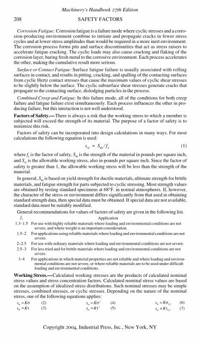
208 SAFETY FACTORS
Corrosion Fatigue: Corrosion fatigue is a failure mode where cyclic stresses and a corro-sion-producing environment combine to initiate and propagate cracks in fewer stresscycles and at lower stress amplitudes than would be required in a more inert environment.The corrosion process forms pits and surface discontinuities that act as stress raisers toaccelerate fatigue cracking. The cyclic loads may also cause cracking and flaking of thecorrosion layer, baring fresh metal to the corrosive environment. Each process acceleratesthe other, making the cumulative result more serious.
Surface or Contact Fatigue: Surface fatigue failure is usually associated with rollingsurfaces in contact, and results in pitting, cracking, and spalling of the contacting surfacesfrom cyclic Hertz contact stresses that cause the maximum values of cyclic shear stressesto be slightly below the surface. The cyclic subsurface shear stresses generate cracks thatpropagate to the contacting surface, dislodging particles in the process.
Combined Creep and Fatigue: In this failure mode, all of the conditions for both creepfailure and fatigue failure exist simultaneously. Each process influences the other in pro-ducing failure, but this interaction is not well understood.
Factors of Safety.—There is always a risk that the working stress to which a member issubjected will exceed the strength of its material. The purpose of a factor of safety is tominimize this risk.
Factors of safety can be incorporated into design calculations in many ways. For mostcalculations the following equation is used:
(1)
where fs is the factor of safety, Sm is the strength of the material in pounds per square inch,and Sw is the allowable working stress, also in pounds per square inch. Since the factor ofsafety is greater than 1, the allowable working stress will be less than the strength of thematerial.
In general, Sm is based on yield strength for ductile materials, ultimate strength for brittlematerials, and fatigue strength for parts subjected to cyclic stressing. Most strength valuesare obtained by testing standard specimens at 68°F. in normal atmospheres. If, however,the character of the stress or environment differs significantly from that used in obtainingstandard strength data, then special data must be obtained. If special data are not available,standard data must be suitably modified.
General recommendations for values of factors of safety are given in the following list.
Working Stress.—Calculated working stresses are the products of calculated nominalstress values and stress concentration factors. Calculated nominal stress values are basedon the assumption of idealized stress distributions. Such nominal stresses may be simplestresses, combined stresses, or cyclic stresses. Depending on the nature of the nominalstress, one of the following equations applies:
fs Application1.3–1.5 For use with highly reliable materials where loading and environmental conditions are not
severe, and where weight is an important consideration.1.5–2 For applications using reliable materials where loading and environmental conditions are not
severe.2–2.5 For use with ordinary materials where loading and environmental conditions are not severe.2.5–3 For less tried and for brittle materials where loading and environmental conditions are not
severe.3–4 For applications in which material properties are not reliable and where loading and environ-
mental conditions are not severe, or where reliable materials are to be used under difficult loading and environmental conditions.
sw =Kσ (2) sw =Kτ (3)
sw =Kσ′ (4) sw =Kτ′ (5)
sw =Kσcy (6) sw =Kτcy (7)
sw Sm fs⁄=
Machinery's Handbook 27th Edition
Copyright 2004, Industrial Press, Inc., New York, NY
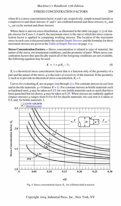
STRESS CONCENTRATION FACTORS 209
where K is a stress concentration factor; σ and τ are, respectively, simple normal (tensile orcompressive) and shear stresses; σ′ and τ′ are combined normal and shear stresses; σcy andτcy are cyclic normal and shear stresses.
Where there is uneven stress distribution, as illustrated in the table (on page 213) of sim-ple stresses for Cases 3, 4 and 6, the maximum stress is the one to which the stress concen-tration factor is applied in computing working stresses. The location of the maximumstress in each case is discussed under the section Simple Stresses and the formulas for thesemaximum stresses are given in the Table of Simple Stresses on page 213.
Stress Concentration Factors.—Stress concentration is related to type of material, thenature of the stress, environmental conditions, and the geometry of parts. When stress con-centration factors that specifically match all of the foregoing conditions are not available,the following equation may be used:
(8)
Kt is a theoretical stress concentration factor that is a function only of the geometry of apart and the nature of the stress; q is the index of sensitivity of the material. If the geometryis such as to provide no theoretical stress concentration, Kt = 1.
Curves for evaluating Kt are on pages 209 through 212. For constant stresses in cast ironand in ductile materials, q = 0 (hence K = 1). For constant stresses in brittle materials suchas hardened steel, q may be taken as 0.15; for very brittle materials such as steels that havebeen quenched but not drawn, q may be taken as 0.25. When stresses are suddenly applied(impact stresses) q ranges from 0.4 to 0.6 for ductile materials; for cast iron it is taken as0.5; and, for brittle materials, 1.
Fig. 4. Stress-concentration factor, Kt , for a filleted shaft in tension
K 1 q Kt 1–( )+=
r
dD
D/d
F F
2.5
2.0
1.5
1.0
Stre
ss-C
once
ntra
tion
fac
tor,
Kt
1.01
1.10
1.2
1.52
1.05
0 0.05 0.10 0.15 0.20 0.25 0.30
r/d
Machinery's Handbook 27th Edition
Copyright 2004, Industrial Press, Inc., New York, NY
LIVE GRAPHClick here to view
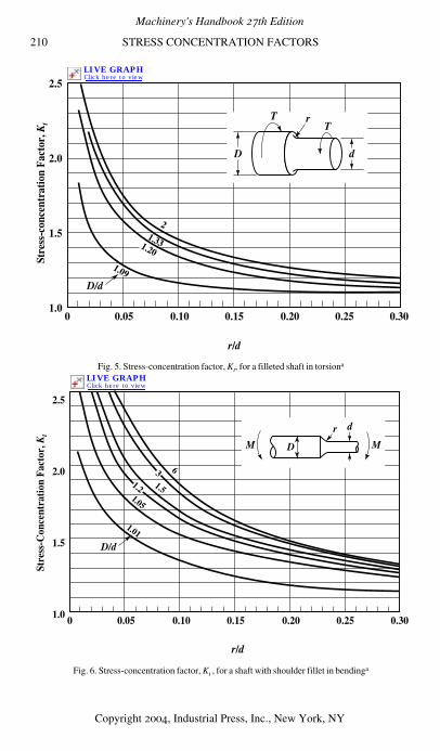
210 STRESS CONCENTRATION FACTORS
Fig. 5. Stress-concentration factor, Kt, for a filleted shaft in torsiona
Fig. 6. Stress-concentration factor, Kt , for a shaft with shoulder fillet in bendinga
2.5
2.0
1.5
1.00 0.05 0.10 0.15
r/d
0.20 0.25 0.30
D/d
21.331.20
1.09
TT
r
D d
Stre
ss-c
once
ntra
tion
Fact
or, K
t
2.5
2.0
1.5
1.0 0 0.05 0.10 0.15 0.20 0.25 0.30
D/d
6
1.51.05
1.01
DM M
dr
Stre
ss-C
once
ntra
tion
Fac
tor,
Kt
31.2
r/d
Machinery's Handbook 27th Edition
Copyright 2004, Industrial Press, Inc., New York, NY
LIVE GRAPHClick here to view
LIVE GRAPHClick here to view
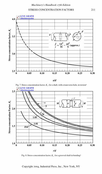
STRESS CONCENTRATION FACTORS 211
Fig. 7. Stress-concentration factor, Kt , for a shaft, with a transverse hole, in torsiona
Fig. 8. Stress-concentration factor, Kt , for a grooved shaft in bendinga
4.0
3.5
3.0
2.5
Stre
ss-c
once
ntra
tion
fact
or, K
t
0 0.05 0.10 0.15 0.20 0.25 0.30
T T
da
Jc
πd3
16ad2
6 (approx.)–=
a/d
2.5
2.0
1.5
1.0
Stre
ss-c
once
ntra
tion
Fac
tor,
Kt
0 0.05 0.10
∞
0.15
r/d
5
1.05
1.01
0.20 0.25 0.30
D/d
1.10
M Md
r
D
Machinery's Handbook 27th Edition
Copyright 2004, Industrial Press, Inc., New York, NY
LIVE GRAPHClick here to view
LIVE GRAPHClick here to view
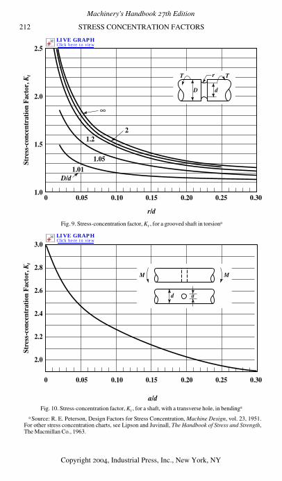
212 STRESS CONCENTRATION FACTORS
Fig. 9. Stress-concentration factor, Kt , for a grooved shaft in torsiona
Fig. 10. Stress-concentration factor, Kt , for a shaft, with a transverse hole, in bendinga
a Source: R. E. Peterson, Design Factors for Stress Concentration, Machine Design, vol. 23, 1951.For other stress concentration charts, see Lipson and Juvinall, The Handbook of Stress and Strength,The Macmillan Co., 1963.
2.5
2.0
1.5
1.0
Stre
ss-c
once
ntra
tion
Fac
tor,
Kt
0 0.05 0.10
∞
0.15
r/d
21.2
1.05
0.20 0.25 0.30
D/d
d
r
D
T T
1.01
3.0
2.8
2.6
2.4
2.2
2.0
Stre
ss-c
once
ntra
tion
Fac
tor,
Kt
0 0.05 0.10 0.15 0.20 0.25 0.30
d a
M M
a/d
Machinery's Handbook 27th Edition
Copyright 2004, Industrial Press, Inc., New York, NY
LIVE GRAPHClick here to view
LIVE GRAPHClick here to view
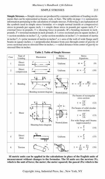
SIMPLE STRESSES 213
Simple Stresses.—Simple stresses are produced by constant conditions of loading on ele-ments that can be represented as beams, rods, or bars. The table on page 213 summarizesinformation pertaining to the calculation of simple stresses. Following is an explanation ofthe symbols used in simple stress formulae: σ = simple normal (tensile or compressive)stress in pounds per square inch; τ = simple shear stress in pounds per square inch; F =external force in pounds; V = shearing force in pounds; M = bending moment in inch-pounds; T = torsional moment in inch-pounds; A = cross-sectional area in square inches; Z= section modulus in inches3; Zp = polar section modulus in inches3; I = moment of inertiain inches4; J = polar moment of inertia in inches4; a = area of the web of wide flange and Ibeams in square inches; y = perpendicular distance from axis through center of gravity ofcross-sectional area to stressed fiber in inches; c = radial distance from center of gravity tostressed fiber in inches.
SI metric units can be applied in the calculations in place of the English units ofmeasurement without changes to the formulas. The SI units are the newton (N),which is the unit of force; the meter; the meter squared; the pascal (Pa) which is the
Table 2. Table of Simple Stresses
Case Type ofLoading Illustration Stress
DistributionStress
Equations
1 Directtension Uniform (9)
2 Directcompression Uniform (10)
3 Bending
Bending moment diagram Neutral plane
(11)
4 Shear
Shearing force diagramNeutral plane
For beams of rectangular cross-section:
(12)
For beams of solid circular cross-section:
(13)
For wide flange and I beams (approximately):
(14)
5 Directshear Uniform (15)
6 Torsion (16)
σ FA---=
σ FA---–=
σ MZ-----± My
I--------±= =
τ 3V2A-------=
τ 4V3A-------=
τ Va---=
τ FA---=
τ TZp------ Tc
J------= =
Machinery's Handbook 27th Edition
Copyright 2004, Industrial Press, Inc., New York, NY
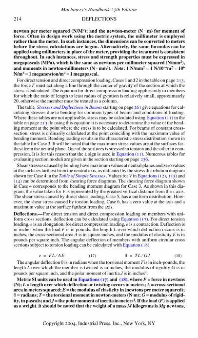
214 DEFLECTIONS
newton per meter squared (N/M2); and the newton-meter (N · m) for moment offorce. Often in design work using the metric system, the millimeter is employedrather than the meter. In such instances, the dimensions can be converted to metersbefore the stress calculations are begun. Alternatively, the same formulas can beapplied using millimeters in place of the meter, providing the treatment is consistentthroughout. In such instances, stress and strength properties must be expressed inmegapascals (MPa), which is the same as newtons per millimeter squared (N/mm2),and moments in newton-millimeters (N · mm2). Note: 1 N/mm2 = 1 N/10−6m2 = 106
N/m2 = 1 meganewton/m2 = 1 megapascal.For direct tension and direct compression loading, Cases 1 and 2 in the table on page 213,
the force F must act along a line through the center of gravity of the section at which thestress is calculated. The equation for direct compression loading applies only to membersfor which the ratio of length to least radius of gyration is relatively small, approximately20, otherwise the member must be treated as a column.
The table Stresses and Deflections in Beams starting on page 261 give equations for cal-culating stresses due to bending for common types of beams and conditions of loading.Where these tables are not applicable, stress may be calculated using Equation (11) in thetable on page 213. In using this equation it is necessary to determine the value of the bend-ing moment at the point where the stress is to be calculated. For beams of constant cross-section, stress is ordinarily calculated at the point coinciding with the maximum value ofbending moment. Bending loading results in the characteristic stress distribution shown inthe table for Case 3. It will be noted that the maximum stress values are at the surfaces far-thest from the neutral plane. One of the surfaces is stressed in tension and the other in com-pression. It is for this reason that the ± sign is used in Equation (11). Numerous tables forevaluating section moduli are given in the section starting on page 236.
Shear stresses caused by bending have maximum values at neutral planes and zero valuesat the surfaces farthest from the neutral axis, as indicated by the stress distribution diagramshown for Case 4 in the Table of Simple Stresses . Values for V in Equations (12), (13) and(14) can be determined from shearing force diagrams. The shearing force diagram shownin Case 4 corresponds to the bending moment diagram for Case 3. As shown in this dia-gram, the value taken for V is represented by the greatest vertical distance from the x axis.The shear stress caused by direct shear loading, Case 5, has a uniform distribution. How-ever, the shear stress caused by torsion loading, Case 6, has a zero value at the axis and amaximum value at the surface farthest from the axis.
Deflections.—For direct tension and direct compression loading on members with uni-form cross sections, deflection can be calculated using Equation (17). For direct tensionloading, e is an elongation; for direct compression loading, e is a contraction. Deflection isin inches when the load F is in pounds, the length L over which deflection occurs is ininches, the cross-sectional area A is in square inches, and the modulus of elasticity E is inpounds per square inch. The angular deflection of members with uniform circular crosssections subject to torsion loading can be calculated with Equation (18).
The angular deflection θ is in radians when the torsional moment T is in inch-pounds, thelength L over which the member is twisted is in inches, the modulus of rigidity G is inpounds per square inch, and the polar moment of inertia J is in inches4.
Metric SI units can be used in Equations (17) and (18), where F = force in newtons(N); L = length over which deflection or twisting occurs in meters; A = cross-sectionalarea in meters squared; E = the modulus of elasticity in (newtons per meter squared);θ = radians; T = the torsional moment in newton-meters (N·m); G = modulus of rigid-ity, in pascals; and J = the polar moment of inertia in meters4. If the load (F) is appliedas a weight, it should be noted that the weight of a mass M kilograms is Mg newtons,
(17) (18)e FL AE⁄= θ TL GJ⁄=
Machinery's Handbook 27th Edition
Copyright 2004, Industrial Press, Inc., New York, NY
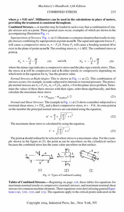
COMBINED STRESS 215
where g = 9.81 m/s2. Millimeters can be used in the calculations in place of meters,providing the treatment is consistent throughout.Combined Stresses.—A member may be loaded in such a way that a combination of sim-ple stresses acts at a point. Three general cases occur, examples of which are shown in theaccompanying illustration Fig. 11.
Superposition of Stresses: Fig. 11 at (1) illustrates a common situation that results in sim-ple stresses combining by superposition at points a and b. The equal and opposite forces F1will cause a compressive stress σ1 = − F1/A. Force F2 will cause a bending moment M toexist in the plane of points a and b. The resulting stress σ2 = ± M/Z. The combined stress atpoint a,
where the minus sign indicates a compressive stress and the plus sign a tensile stress. Thus,the stress at a will be compressive and at b either tensile or compressive depending onwhich term in the equation for σb ′ has the greatest value.
Normal Stresses at Right Angles: This is shown in Fig. 11 at (2). This combination ofstresses occurs, for example, in tanks subjected to internal or external pressure. The princi-ple normal stresses are σx = F1/A1, σy = F2/A2, and σz = 0 in this plane stress problem. Deter-mine the values of these three stresses with their signs, order them algebraically, and thencalculate the maximum shear stress:
(21)
Normal and Shear Stresses: The example in Fig. 11 at (3) shows a member subjected to atorsional shear stress, τ = T/Zp, and a direct compressive stress, σ = − F/A. At some point aon the member the principal normal stresses are calculated using the equation,
(22)
The maximum shear stress is calculated by using the equation,
(23)
The point a should ordinarily be selected where stress is a maximum value. For the exam-ple shown in the figure at (3), the point a can be anywhere on the cylindrical surfacebecause the combined stress has the same value anywhere on that surface.
Fig. 11. Types of Combined Loading
Tables of Combined Stresses.—Beginning on page 216, these tables list equations formaximum nominal tensile or compressive (normal) stresses, and maximum nominal shearstresses for common machine elements. These equations were derived using general Equa-tions (19), (20), (22), and (23). The equations apply to the critical points indicated on the
(19) and at b, (20)σa′
F1
A------– M
Z-----–= σb
′
F1
A------– M
Z-----+=
τ σlargest σsmallest–( ) 2⁄=
σ′ σ2--- σ
2---⎝ ⎠⎛ ⎞ 2
τ2+±=
τ′ σ2---⎝ ⎠⎛ ⎞ 2
τ2+=
Machinery's Handbook 27th Edition
Copyright 2004, Industrial Press, Inc., New York, NY

216 COMBINED STRESS
figures. Cases 1, 2, 3, and 4 are cantilever beams. These may be loaded with a combinationof a vertical and horizontal force, or by a single oblique force. If the single oblique force Fand the angle θ are given, then horizontal and vertical forces can be calculated using theequations Fx = F cos θ and Fy = F sin θ. In cases 9 and 10 of the table, the equations for σa ′can give a tensile and a compressive stress because of the ± sign in front of the radical.Equations involving direct compression are valid only if machine elements have relativelyshort lengths with respect to their sections, otherwise column equations apply.
Calculation of Worst Stress Condition: Stress failure can occur at any critical point ifeither the tensile, compressive, or shear stress properties of the material are exceeded bythe corresponding working stress. It is necessary to evaluate the factor of safety for eachpossible failure condition.
The following rules apply to calculations using equations in the Table of Simple Stresseson page 213, and to calculations based on Equations (19) and (20). Rule 1: For every cal-culated normal stress there is a corresponding induced shear stress; the value of the shearstress is equal to half that of the normal stress. Rule 2: For every calculated shear stressthere is a corresponding induced normal stress; the value of the normal stress is equal tothat of the shear stress. The tables of combined stress formulas, below, include equationsfor calculating both maximum nominal tensile or compressive stresses, and maximumnominal shear stresses.
Formulas for Combined Stresses
(1) Circular Cantilever Beam in Direct Compression and Bending:
(2) Circular Cantilever Beam in Direct Tension and Bending:
(3) Rectangular Cantilever Beam in Direct Compression and Bending:
Type of Beamand Loading
Maximum NominalTensile or Compressive Stress
Maximum NominalShear Stress
Type of Beamand Loading
Maximum NominalTensile or Compressive Stress
Maximum NominalShear Stress
Type of Beamand Loading
Maximum NominalTensile or Compressive Stress
Maximum NominalShear Stress
σa′
1.273
d2
-------------8LFy
d------------- Fx–⎝ ⎠⎛ ⎞= τa
′ 0.5σa′=
σb′
1.273
d2
-------------8LFy
d------------- Fx+⎝ ⎠⎛ ⎞–= τb
′ 0.5σb′=
σa′
1.273
d2
------------- Fx
8LFy
d-------------+⎝ ⎠
⎛ ⎞ = τa′ 0.5σa
′=
σb′
1.273
d2
------------- Fx
8LFy
d-------------–⎝ ⎠
⎛ ⎞= τb′ 0.5σb
′=
σa′
1bh------
6LFy
h------------- Fx–⎝ ⎠⎛ ⎞= τa
′ 0.5σa′=
σb′
1bh------
6LFy
h------------- Fx+⎝ ⎠⎛ ⎞–= τb
′ 0.5σb′=
Machinery's Handbook 27th Edition
Copyright 2004, Industrial Press, Inc., New York, NY
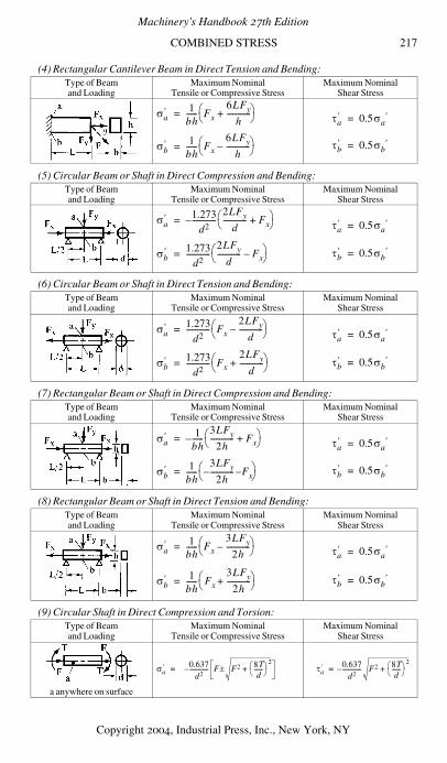
COMBINED STRESS 217
(4) Rectangular Cantilever Beam in Direct Tension and Bending:
(5) Circular Beam or Shaft in Direct Compression and Bending:
(6) Circular Beam or Shaft in Direct Tension and Bending:
(7) Rectangular Beam or Shaft in Direct Compression and Bending:
(8) Rectangular Beam or Shaft in Direct Tension and Bending:
(9) Circular Shaft in Direct Compression and Torsion:
Type of Beamand Loading
Maximum NominalTensile or Compressive Stress
Maximum NominalShear Stress
Type of Beamand Loading
Maximum NominalTensile or Compressive Stress
Maximum NominalShear Stress
Type of Beamand Loading
Maximum NominalTensile or Compressive Stress
Maximum NominalShear Stress
Type of Beamand Loading
Maximum NominalTensile or Compressive Stress
Maximum NominalShear Stress
Type of Beamand Loading
Maximum NominalTensile or Compressive Stress
Maximum NominalShear Stress
Type of Beamand Loading
Maximum NominalTensile or Compressive Stress
Maximum NominalShear Stress
a anywhere on surface
σa′
1bh------ Fx
6LFy
h-------------+⎝ ⎠
⎛ ⎞= τa′ 0.5σa
′=
σb′
1bh------ Fx
6LFy
h-------------–⎝ ⎠
⎛ ⎞= τb′ 0.5σb
′=
σa′
1.273d2
-------------–2LFy
d------------- Fx+⎝ ⎠⎛ ⎞= τa
′ 0.5σa′=
σb′
1.273d2
-------------2LFy
d------------- Fx–⎝ ⎠⎛ ⎞= τb
′ 0.5σb′=
σa′
1.273d2
------------- Fx
2LFy
d-------------–⎝ ⎠
⎛ ⎞= τa′ 0.5σa
′=
σb′
1.273d2
------------- Fx
2LFy
d-------------+⎝ ⎠
⎛ ⎞= τb′ 0.5σb
′=
σa′
1bh------–
3LFy
2h------------- Fx+⎝ ⎠⎛ ⎞= τa
′ 0.5σa′=
σb′
1bh------
3LFy
2h------------- F– x–⎝ ⎠
⎛ ⎞= τb′ 0.5σb
′=
σa′
1bh------ Fx
3LFy
2h-------------–⎝ ⎠
⎛ ⎞= τa′ 0.5σa
′=
σb′
1bh------ Fx
3LFy
2h-------------+⎝ ⎠
⎛ ⎞= τb′ 0.5σb
′=
σa′
0.637d2
-------------– F F2 8Td
------⎝ ⎠⎛ ⎞
2+±= τa
′0.637
d2-------------– F2 8T
d------⎝ ⎠⎛ ⎞
2+=
Machinery's Handbook 27th Edition
Copyright 2004, Industrial Press, Inc., New York, NY
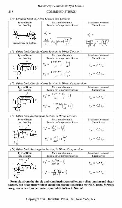
218 COMBINED STRESS
(10) Circular Shaft in Direct Tension and Torsion:
(11) Offset Link, Circular Cross Section, in Direct Tension:
(12) Offset Link, Circular Cross Section, in Direct Compression:
(13) Offset Link, Rectangular Section, in Direct Tension:
(14) Offset Link, Rectangular Section, in Direct Compression:
Formulas from the simple and combined stress tables, as well as tension and shearfactors, can be applied without change in calculations using metric SI units. Stressesare given in newtons per meter squared (N/m2) or in N/mm2.
Type of Beamand Loading
Maximum NominalTensile or Compressive Stress
Maximum NominalShear Stress
a anywhere on surface
Type of Beamand Loading
Maximum NominalTensile or Compressive Stress
Maximum NominalShear Stress
Type of Beamand Loading
Maximum NominalTensile or Compressive Stress
Maximum NominalShear Stress
Type of Beamand Loading
Maximum NominalTensile or Compressive Stress
Maximum NominalShear Stress
Type of Beamand Loading
Maximum NominalTensile or Compressive Stress
Maximum NominalShear Stress
σa′
0.637d2
------------- F F2 8Td
------⎝ ⎠⎛ ⎞ 2
+±
=τa′
0.637d2
------------- F2 8Td
------⎝ ⎠⎛ ⎞ 2
+
=
σa′
1.273Fd2
----------------- 1 8ed
------–⎝ ⎠⎛ ⎞= τa
′ 0.5σa′=
σb′
1.273Fd2
----------------- 1 8ed
------+⎝ ⎠⎛ ⎞= τb
′ 0.5σb′=
σa ′1.273F
d2----------------- 8e
d------ 1–⎝ ⎠⎛ ⎞= τa
′ 0.5σa′=
σb ′1.273F
d2-----------------– 8e
d------ 1+⎝ ⎠⎛ ⎞= τb
′ 0.5σb′=
σa ′Fbh------ 1 6e
h------–⎝ ⎠
⎛ ⎞= τa′ 0.5σa
′=
σb ′Fbh------ 1 6e
h------+
⎝ ⎠⎛ ⎞= τb
′ 0.5σb′=
σa ′Fbh------ 6e
h------ 1–⎝ ⎠⎛ ⎞= τa
′ 0.5σa′=
σb ′Fbh------– 6e
h------ 1+⎝ ⎠⎛ ⎞= τb
′ 0.5σb′=
Machinery's Handbook 27th Edition
Copyright 2004, Industrial Press, Inc., New York, NY
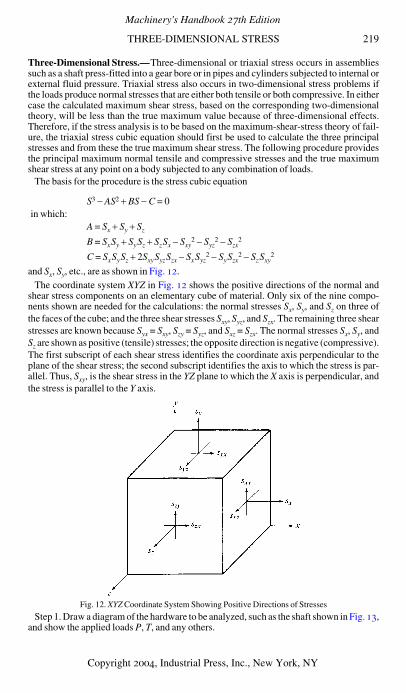
THREE-DIMENSIONAL STRESS 219
Three-Dimensional Stress.—Three-dimensional or triaxial stress occurs in assembliessuch as a shaft press-fitted into a gear bore or in pipes and cylinders subjected to internal orexternal fluid pressure. Triaxial stress also occurs in two-dimensional stress problems ifthe loads produce normal stresses that are either both tensile or both compressive. In eithercase the calculated maximum shear stress, based on the corresponding two-dimensionaltheory, will be less than the true maximum value because of three-dimensional effects.Therefore, if the stress analysis is to be based on the maximum-shear-stress theory of fail-ure, the triaxial stress cubic equation should first be used to calculate the three principalstresses and from these the true maximum shear stress. The following procedure providesthe principal maximum normal tensile and compressive stresses and the true maximumshear stress at any point on a body subjected to any combination of loads.
The basis for the procedure is the stress cubic equation
and Sx, Sy, etc., are as shown in Fig. 12.The coordinate system XYZ in Fig. 12 shows the positive directions of the normal and
shear stress components on an elementary cube of material. Only six of the nine compo-nents shown are needed for the calculations: the normal stresses Sx, Sy, and Sz on three ofthe faces of the cube; and the three shear stresses Sxy, Syz, and Szx. The remaining three shearstresses are known because Syx = Sxy, Szy = Syz, and Sxz = Szx. The normal stresses Sx, Sy, andSz are shown as positive (tensile) stresses; the opposite direction is negative (compressive).The first subscript of each shear stress identifies the coordinate axis perpendicular to theplane of the shear stress; the second subscript identifies the axis to which the stress is par-allel. Thus, Sxy, is the shear stress in the YZ plane to which the X axis is perpendicular, andthe stress is parallel to the Y axis.
Fig. 12. XYZ Coordinate System Showing Positive Directions of Stresses
Step 1. Draw a diagram of the hardware to be analyzed, such as the shaft shown in Fig. 13,and show the applied loads P, T, and any others.
S3 − AS2 + BS − C = 0in which:
A = Sx + Sy + Sz
B = SxSy + SySz + SzSx − Sxy2 − Syz
2 − Szx2
C = SxSySz + 2SxySyzSzx − SxSyz2 − SySzx
2 − SzSxy2
Machinery's Handbook 27th Edition
Copyright 2004, Industrial Press, Inc., New York, NY
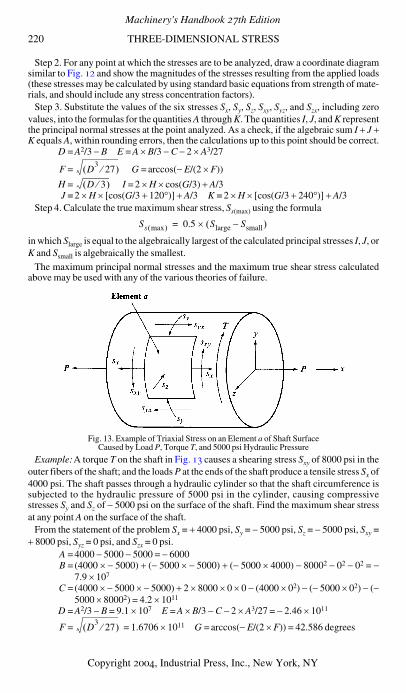
220 THREE-DIMENSIONAL STRESS
Step 2. For any point at which the stresses are to be analyzed, draw a coordinate diagramsimilar to Fig. 12 and show the magnitudes of the stresses resulting from the applied loads(these stresses may be calculated by using standard basic equations from strength of mate-rials, and should include any stress concentration factors).
Step 3. Substitute the values of the six stresses Sx, Sy, Sz, Sxy, Syz, and Szx, including zerovalues, into the formulas for the quantities A through K. The quantities I, J, and K representthe principal normal stresses at the point analyzed. As a check, if the algebraic sum I + J +K equals A, within rounding errors, then the calculations up to this point should be correct.
D =A2/3 − B E =A × B/3 − C − 2 × A3/27
F = G =arccos(− E/(2 × F))
H = I =2 × H × cos(G/3) + A/3J =2 × H × [cos(G/3 + 120°)] + A/3 K =2 × H × [cos(G/3 + 240°)] + A/3
Step 4. Calculate the true maximum shear stress, Ss(max) using the formula
in which Slarge is equal to the algebraically largest of the calculated principal stresses I, J, orK and Ssmall is algebraically the smallest.
The maximum principal normal stresses and the maximum true shear stress calculatedabove may be used with any of the various theories of failure.
Fig. 13. Example of Triaxial Stress on an Element a of Shaft SurfaceCaused by Load P, Torque T, and 5000 psi Hydraulic Pressure
Example:A torque T on the shaft in Fig. 13 causes a shearing stress Sxy of 8000 psi in theouter fibers of the shaft; and the loads P at the ends of the shaft produce a tensile stress Sx of4000 psi. The shaft passes through a hydraulic cylinder so that the shaft circumference issubjected to the hydraulic pressure of 5000 psi in the cylinder, causing compressivestresses Sy and Sz of − 5000 psi on the surface of the shaft. Find the maximum shear stressat any point A on the surface of the shaft.
From the statement of the problem Sx = + 4000 psi, Sy = − 5000 psi, Sz = − 5000 psi, Sxy =+ 8000 psi, Syz = 0 psi, and Szx = 0 psi.
A =4000 − 5000 − 5000 = − 6000B =(4000 × − 5000) + (− 5000 × − 5000) + (− 5000 × 4000) − 80002 − 02 − 02 = −
7.9 × 10⁷
C =(4000 × − 5000 × − 5000) + 2 × 8000 × 0 × 0 − (4000 × 02) − (− 5000 × 02) − (−5000 × 80002) = 4.2 × 10¹¹
D =A2/3 − B = 9.1 × 10⁷ E =A × B/3 − C − 2 × A3/27 = − 2.46 × 10¹¹
F = = 1.6706 × 10¹¹ G =arccos(− E/(2 × F)) = 42.586 degrees
D3
27⁄( )
D 3⁄( )
Ss max( ) 0.5 Slarge Ssmall–( )×=
D3
27⁄( )
Machinery's Handbook 27th Edition
Copyright 2004, Industrial Press, Inc., New York, NY
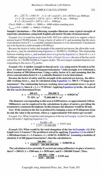
SAMPLE CALCULATIONS 221
H = = 5507.57 I =2 × H × cos(G/3 + A/3 = 8678.8, say, 8680 psiJ =2 × H × [cos(G/3 + 120°)] + A/3 = − 9678.78, say, − 9680 psiK =2 × H [cos(G/3 + 240°)] + A/3 = − 5000 psi
Check: 8680 + (− 9680) + (− 5000) = − 6000 within rounding error.Ss(max) = 0.5 × (8680 − (− 9680)) = 9180 psi
Sample Calculations.—The following examples illustrate some typical strength ofmaterials calculations, using both English and metric SI units of measurement.
Example 1(a):A round bar made from SAE 1025 low carbon steel is to support a directtension load of 50,000 pounds. Using a factor of safety of 4, and assuming that the stressconcentration factor K = 1, a suitable standard diameter is to be determined. Calculationsare to be based on a yield strength of 40,000 psi.
Because the factor of safety and strength of the material are known, the allowable work-ing stress sw may be calculated using Equation (1): 40,000 ⁄4 = 10,000 psi. The relationshipbetween working stress sw and nominal stress σ is given by Equation (2). Since K = 1, σ =10,000 psi. Applying Equation (9) in the Table of Simple Stresses, the area of the bar can besolved for: A = 50,000 ⁄10,000 or 5 square inches. The next largest standard diameter cor-responding to this area is 29⁄16 inches.
Example 1(b):A similar example to that given in 1(a), using metric SI units is as fol-lows. A round steel bar of 300 meganewtons/meter 2 yield strength, is to withstand adirect tension of 200 kilonewtons. Using a safety factor of 4, and assuming that thestress concentration factor K = 1, a suitable diameter is to be determined.
Because the factor of safety and the strength of the material are known, the allow-able working stress sw may be calculated using Equation (1): 300 ⁄4 = 75 mega-new-tons/meter2. The relationship between working stress and nominal stress σ is givenby Equation (2). Since K = 1, σ = 75 MN/m2. Applying Equation (9) in the , the area ofthe bar can be determined from:
The diameter corresponding to this area is 0.058 meters, or approximately 0.06 m.Millimeters can be employed in the calculations in place of meters, providing the
treatment is consistent throughout. In this instance the diameter would be 60 mm.Note: If the tension in the bar is produced by hanging a mass of M kilograms from
its end, the value is Mg newtons, where g = approximately 9.81 meters per second2.Example 2(a):What would the total elongation of the bar in Example 1(a) be if its length
were 60 inches? Applying Equation (17),
Example 2(b):What would be the total elongation of the bar in Example 1(b) if itslength were 1.5 meters? The problem is solved by applying Equation (17) in which F= 200 kilonewtons; L = 1.5 meters; A = π0.062/4 = 0.00283 m2. Assuming a modulus ofelasticity E of 200 giganewtons/meter2, then the calculation is:
The calculation is less unwieldy if carried out using millimeters in place of meters;then F = 200 kN; L = 1500 mm; A = 2830 mm2, and E = 200,000 N/mm2. Thus:
D 3⁄( )
A 200 kN
75 MN m2⁄
------------------------------ 200 000 N,
75 000 000 N m2⁄,,
----------------------------------------------- 0.00267m2= = =
e 50 000, 60×5.157 30 000 000,,×----------------------------------------------- 0.019 inch= =
e 200 000, 1.5×
0.00283 200 000 000 000,,,×------------------------------------------------------------------- 0.000530 m= =
e 200 000, 1500×
2830 200 000,×-------------------------------------- 0.530 mm= =
Machinery's Handbook 27th Edition
Copyright 2004, Industrial Press, Inc., New York, NY

222 SAMPLE CALCULATIONS
Example 3(a):Determine the size for the section of a square bar which is to be held firmlyat one end and is to support a load of 3000 pounds at the outer end. The bar is to be 30 incheslong and is to be made from SAE 1045 medium carbon steel with a yield point of 60,000psi. A factor of safety of 3 and a stress concentration factor of 1.3 are to be used.
From Equation (1) the allowable working stress sw = 60,000 ⁄3 = 20,000 psi. The applica-ble equation relating working stress and nominal stress is Equation (2); hence, σ =20,000 ⁄1.3 = 15,400 psi. The member must be treated as a cantilever beam subject to abending moment of 30 × 3000 or 90,000 inch-pounds. Solving Equation (11) in the for sec-tion modulus: Z = 90,000 ⁄15,400 = 5.85 inch3. The section modulus for a square sectionwith neutral axis equidistant from either side is a3/6, where a is the dimension of the
square, so inches. The size of the bar can therefore be 35⁄16 inches.
Example 3(b):A similar example to that given in Example 3(a), using metric SI unitsis as follows. Determine the size for the section of a square bar which is to be heldfirmly at one end and is to support a load of 1600 kilograms at the outer end. The baris to be 1 meter long, and is to be made from steel with a yield strength of 500 new-tons/mm2. A factor of safety of 3, and a stress concentration factor of 1.3 are to beused. The calculation can be performed using millimeters throughout.
From Equation (1) the allowable working stress sw = 500 N/mm2/3 = 167 N/mm2.The formula relating working stress and nominal stress is Equation (2); hence σ =167 ⁄1.3 = 128 N/mm2. Since a mass of 1600 kg equals a weight of 1600 g newtons,where g = 9.81 meters/second2, the force acting on the bar is 15,700 newtons. Thebending moment on the bar, which must be treated as a cantilever beam, is thus 1000mm × 15,700 N = 15,700,000 N · mm. Solving Equation (11) in the for section modu-lus: Z = M/σ = 15,700,000 ⁄128 = 123,000 mm3. Since the section modulus for a squaresection with neutral axis equidistant from either side is a3/6, where a is the dimensionof the square,
Example 4(a):Find the working stress in a 2-inch diameter shaft through which a trans-verse hole 1⁄4 inch in diameter has been drilled. The shaft is subject to a torsional moment of80,000 inch-pounds and is made from hardened steel so that the index of sensitivity q = 0.2.
The polar section modulus is calculated using the equation shown in the stress concentra-tion curve for a Round Shaft in Torsion with Transverse Hole, Fig. 7, page 211.
The nominal shear stress due to the torsion loading is computed using Equation (16) inthe :
Referring to the previously mentioned stress concentration curve on page 211, Kt is 2.82since d/D is 0.125. The stress concentration factor may now be calculated by means ofEquation (8): K = 1 + 0.2(2.82 − 1) = 1.36. Working stress calculated with Equation (3) issw = 1.36 × 57,200 = 77,800 psi.
Example 4(b):A similar example to that given in 4(a), using metric SI units is as fol-lows. Find the working stress in a 50 mm diameter shaft through which a transversehole 6 mm in diameter has been drilled. The shaft is subject to a torsional moment of8000 newton-meters, and has an index of sensitivity of q = 0.2. If the calculation ismade in millimeters, the torsional moment is 8,000,000 N · mm.
The polar section modulus is calculated using the equation shown in the stress con-centration curve for a Round Shaft in Torsion with Transverse Hole, Fig. 7, page 211:
a 35.13 3.27= =
a 6 123 000,×3 90.4 mm= =
Jc-- Zp
π 23×16
--------------- 22
4 6×------------– 1.4 inches3= = =
τ 80 000, 1.4⁄ 57 200 psi,= =
Machinery's Handbook 27th Edition
Copyright 2004, Industrial Press, Inc., New York, NY
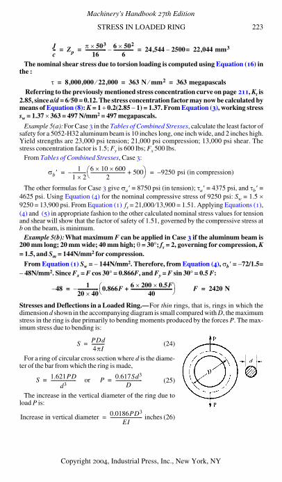
STRESS IN LOADED RING 223
The nominal shear stress due to torsion loading is computed using Equation (16) inthe :
Referring to the previously mentioned stress concentration curve on page 211, Kt is2.85, since a/d = 6 ⁄50 = 0.12. The stress concentration factor may now be calculated bymeans of Equation (8): K = 1 + 0.2(2.85 − 1) = 1.37. From Equation (3), working stresssw = 1.37 × 363 = 497 N/mm2 = 497 megapascals.
Example 5(a):For Case 3 in the Tables of Combined Stresses, calculate the least factor ofsafety for a 5052-H32 aluminum beam is 10 inches long, one inch wide, and 2 inches high.Yield strengths are 23,000 psi tension; 21,000 psi compression; 13,000 psi shear. Thestress concentration factor is 1.5; Fy is 600 lbs; Fx 500 lbs.
From Tables of Combined Stresses, Case 3:
The other formulas for Case 3 give σa ′ = 8750 psi (in tension); τa ′ = 4375 psi, and τb ′ =4625 psi. Using Equation (4) for the nominal compressive stress of 9250 psi: Sw = 1.5 ×9250 = 13,900 psi. From Equation (1) fs = 21,000 ⁄13,900 = 1.51. Applying Equations (1),(4) and (5) in appropriate fashion to the other calculated nominal stress values for tensionand shear will show that the factor of safety of 1.51, governed by the compressive stress atb on the beam, is minimum.
Example 5(b):What maximum F can be applied in Case 3 if the aluminum beam is200 mm long; 20 mm wide; 40 mm high; θ = 30°; fs = 2, governing for compression, K= 1.5, and Sm = 144N/mm2 for compression.
From Equation (1) Sw = − 144N/mm2. Therefore, from Equation (4), σb ′ = −72/1.5=− 48N/mm2. Since Fx = F cos 30° = 0.866F, and Fy = F sin 30° = 0.5 F:
Stresses and Deflections in a Loaded Ring.—For thin rings, that is, rings in which thedimension d shown in the accompanying diagram is small compared with D, the maximumstress in the ring is due primarily to bending moments produced by the forces P. The max-imum stress due to bending is:
(24)
For a ring of circular cross section where d is the diame-ter of the bar from which the ring is made,
(25)
The increase in the vertical diameter of the ring due toload P is:
(26)
Jc--- Zp
π 503×
16------------------ 6 502×
6-----------------– 24 544, 2500– 22 044,= mm3= = =
τ 8 000 000,, 22 000,⁄ 363 N mm2⁄ 363 megapascals= = =
σb ′1
1 2×------------ 6 10× 600×
2------------------------------ 500+⎝ ⎠⎛ ⎞– 9250 psi (in compression)–= =
48– 120 40×------------------ 0.866F 6 200× 0.5F×
40------------------------------------+⎝ ⎠
⎛ ⎞–= F 2420 N=
S PDd4πI-----------=
S 1.621PDd3
---------------------- or= P 0.617Sd3
D-----------------------=
Increase in vertical diameter 0.0186PD3
EI---------------------------- inches=
Machinery's Handbook 27th Edition
Copyright 2004, Industrial Press, Inc., New York, NY
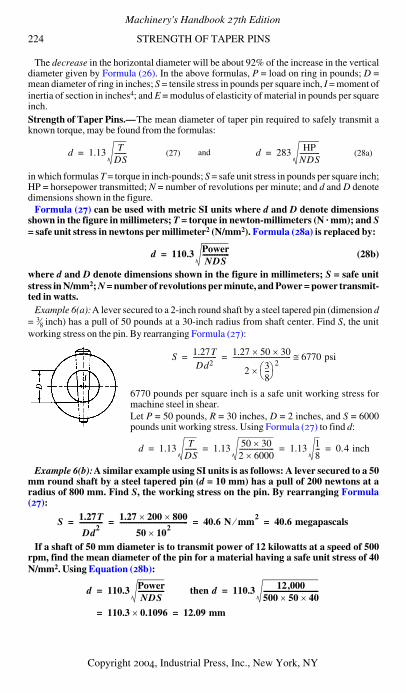
224 STRENGTH OF TAPER PINS
The decrease in the horizontal diameter will be about 92% of the increase in the verticaldiameter given by Formula (26). In the above formulas, P = load on ring in pounds; D =mean diameter of ring in inches; S = tensile stress in pounds per square inch, I = moment ofinertia of section in inches4; and E = modulus of elasticity of material in pounds per squareinch.Strength of Taper Pins.—The mean diameter of taper pin required to safely transmit aknown torque, may be found from the formulas:
in which formulas T = torque in inch-pounds; S = safe unit stress in pounds per square inch;HP = horsepower transmitted; N = number of revolutions per minute; and d and D denotedimensions shown in the figure.
Formula (27) can be used with metric SI units where d and D denote dimensionsshown in the figure in millimeters; T = torque in newton-millimeters (N · mm); and S= safe unit stress in newtons per millimeter2 (N/mm2). Formula (28a) is replaced by:
(28b)
where d and D denote dimensions shown in the figure in millimeters; S = safe unitstress in N/mm2; N = number of revolutions per minute, and Power = power transmit-ted in watts.
Example 6(a):A lever secured to a 2-inch round shaft by a steel tapered pin (dimension d= 3⁄8 inch) has a pull of 50 pounds at a 30-inch radius from shaft center. Find S, the unitworking stress on the pin. By rearranging Formula (27):
6770 pounds per square inch is a safe unit working stress formachine steel in shear.Let P = 50 pounds, R = 30 inches, D = 2 inches, and S = 6000pounds unit working stress. Using Formula (27) to find d:
Example 6(b):A similar example using SI units is as follows: A lever secured to a 50mm round shaft by a steel tapered pin (d = 10 mm) has a pull of 200 newtons at aradius of 800 mm. Find S, the working stress on the pin. By rearranging Formula(27):
If a shaft of 50 mm diameter is to transmit power of 12 kilowatts at a speed of 500rpm, find the mean diameter of the pin for a material having a safe unit stress of 40N/mm2. Using Equation (28b):
(27) and (28a)d 1.13 TDS-------= d 283 HP
NDS------------=
d 110.3 PowerNDS
----------------=
S 1.27TDd2
-------------- 1.27 50× 30×
2 38---⎝ ⎠⎛ ⎞ 2
×----------------------------------- 6770 psi≅= =
d 1.13 TDS------- 1.13 50 30×
2 6000×--------------------- 1.13 1
8--- 0.4 inch= = = =
S 1.27T
Dd2
-------------- 1.27 200× 800×
50 102×
----------------------------------------- 40.6 N mm2⁄ 40.6 megapascals= = = =
d 110.3 PowerNDS
----------------= then d 110.3 12 000,500 50× 40×---------------------------------=
110.3 0.1096×= 12.09 mm=
Machinery's Handbook 27th Edition
Copyright 2004, Industrial Press, Inc., New York, NY

CENTER OF GRAVITY 225
PROPERTIES OF BODIES
Center of Gravity
Center of Gravity.—The center of gravity of a body, volume, area, or line is that point atwhich if the body, volume, area, or line were suspended it would be perfectly balanced inall positions. For symmetrical bodies of uniform material it is at the geometric center. Thecenter of gravity of a uniform round rod, for example, is at the center of its diameter half-way along its length; the center of gravity of a sphere is at the center of the sphere. For sol-ids, areas, and arcs that are not symmetrical, the determination of the center of gravity maybe made experimentally or may be calculated by the use of formulas.
The tables that follow give such formulas for some of the more important shapes. Formore complicated and unsymmetrical shapes the methods outlined on page 231 may beused.
Example:A piece of wire is bent into the form of a semi-circular arc of 10-inch radius.How far from the center of the arc is the center of gravity located?
Accompanying the Circular Arc diagram on page 226 is a formula for the distance fromthe center of gravity of an arc to the center of the arc: a = 2r ÷ π. Therefore,
Formulas for Center of Gravity
Triangle:
Perimeter or Area of a Parallelogram :
PerimeterIf A, B and C are the middle points of the sides of
the triangle, then the center of gravity is at the cen-ter of the circle that can be inscribed in triangle ABC. The distance d of the center of gravity from side a is:
where h is the height perpendicular to a.
AreaThe center of gravity is at the intersection of
lines AD and BE, which bisect the sides BC and AC. The perpendicular distance from the center of gravity to any one of the sides is equal to one-third the height perpendicular to that side. Hence, a = h ÷ 3.
The center of gravity is at the intersection of the diagonals.
a 2 10× 3.1416÷ 6.366 inches= =
d h b c+( )
2 a b c+ +( )-----------------------------=
Machinery's Handbook 27th Edition
Copyright 2004, Industrial Press, Inc., New York, NY
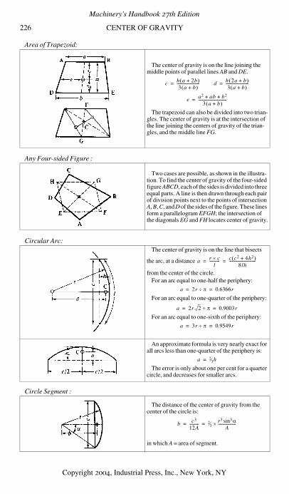
226 CENTER OF GRAVITY
Area of Trapezoid:
Any Four-sided Figure :
Circular Arc:
Circle Segment :
The center of gravity is on the line joining the middle points of parallel lines AB and DE.
The trapezoid can also be divided into two trian-gles. The center of gravity is at the intersection of the line joining the centers of gravity of the trian-gles, and the middle line FG.
Two cases are possible, as shown in the illustra-tion. To find the center of gravity of the four-sided figure ABCD, each of the sides is divided into three equal parts. A line is then drawn through each pair of division points next to the points of intersection A, B, C, and D of the sides of the figure. These lines form a parallelogram EFGH; the intersection of the diagonals EG and FH locates center of gravity.
The center of gravity is on the line that bisects
the arc, at a distance
from the center of the circle.For an arc equal to one-half the periphery:
For an arc equal to one-quarter of the periphery:
For an arc equal to one-sixth of the periphery:
An approximate formula is very nearly exact for all arcs less than one-quarter of the periphery is:
The error is only about one per cent for a quarter circle, and decreases for smaller arcs.
The distance of the center of gravity from the center of the circle is:
in which A = area of segment.
c h a 2b+( )
3 a b+( )------------------------= d h 2a b+( )
3 a b+( )------------------------=
e a2 ab b2+ +3 a b+( )
------------------------------=
a r c×
l----------- c c2 4h2+( )
8lh----------------------------= =
a 2r π÷ 0.6366r= =
a 2r 2 π÷ 0.9003r= =
a 3r π÷ 0.9549r= =
a 2⁄3h=
b c3
12A---------- 2⁄3
r3 αsin3
A-------------------×= =
Machinery's Handbook 27th Edition
Copyright 2004, Industrial Press, Inc., New York, NY
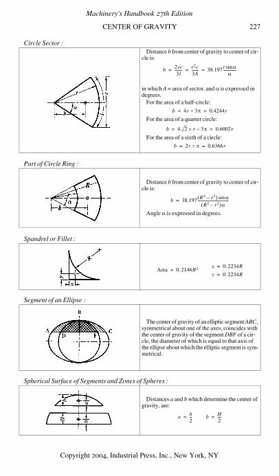
CENTER OF GRAVITY 227
Circle Sector :
Part of Circle Ring :
Spandrel or Fillet :
Segment of an Ellipse :
Spherical Surface of Segments and Zones of Spheres :
Distance b from center of gravity to center of cir-cle is:
in which A = area of sector, and α is expressed in degrees.
For the area of a half-circle:
For the area of a quarter circle:
For the area of a sixth of a circle:
Distance b from center of gravity to center of cir-cle is:
Angle α is expressed in degrees.
The center of gravity of an elliptic segment ABC, symmetrical about one of the axes, coincides with the center of gravity of the segment DBF of a cir-cle, the diameter of which is equal to that axis of the ellipse about which the elliptic segment is sym-metrical.
Distances a and b which determine the center of gravity, are:
b 2rc3l
-------- r2c3A-------- 38.197r αsin
α--------------= = =
b 4r 3π÷ 0.4244r= =
b 4 2 r× 3π÷ 0.6002r= =
b 2r π÷ 0.6366r= =
b 38.197 R3 r3–( ) αsinR2 r2–( )α
----------------------------------=
Area 0.2146R2=x 0.2234R=
y 0.2234R=
a h2---= b H
2----=
Machinery's Handbook 27th Edition
Copyright 2004, Industrial Press, Inc., New York, NY
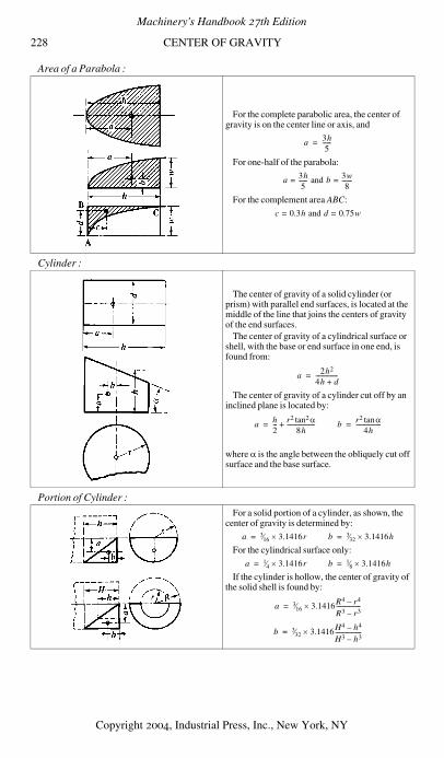
228 CENTER OF GRAVITY
Area of a Parabola :
Cylinder :
Portion of Cylinder :
For the complete parabolic area, the center of gravity is on the center line or axis, and
For one-half of the parabola:
For the complement area ABC:
The center of gravity of a solid cylinder (or prism) with parallel end surfaces, is located at the middle of the line that joins the centers of gravity of the end surfaces.
The center of gravity of a cylindrical surface or shell, with the base or end surface in one end, is found from:
The center of gravity of a cylinder cut off by an inclined plane is located by:
where α is the angle between the obliquely cut off surface and the base surface.
For a solid portion of a cylinder, as shown, the center of gravity is determined by:
For the cylindrical surface only:
If the cylinder is hollow, the center of gravity of the solid shell is found by:
a 3h5
------=
a 3h5
------= and b 3w8
-------=
c 0.3h= and d 0.75w=
a 2h2
4h d+---------------=
a h2--- r2 αtan2
8h-------------------+= b r2 αtan
4h-----------------=
a 3⁄16 3.1416r×= b 3⁄32 3.1416h×=
a 1⁄4 3.1416r×= b 1⁄8 3.1416h×=
a 3⁄16 3.1416R4 r4–R3 r3–-----------------×=
b 3⁄32 3.1416H4 h4–H3 h3–------------------×=
Machinery's Handbook 27th Edition
Copyright 2004, Industrial Press, Inc., New York, NY
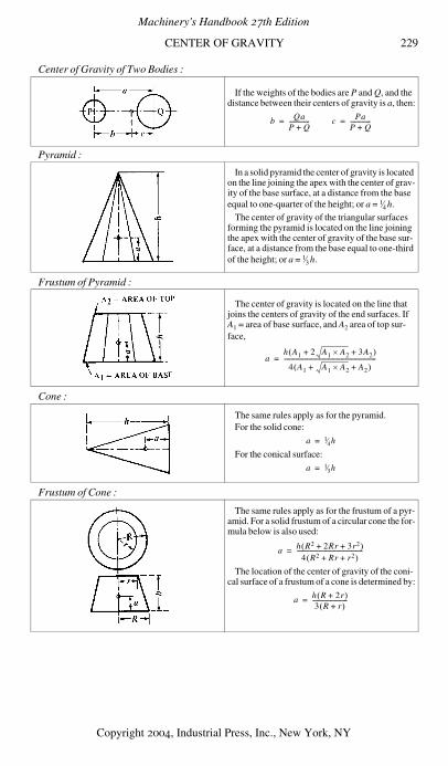
CENTER OF GRAVITY 229
Center of Gravity of Two Bodies :
Pyramid :
Frustum of Pyramid :
Cone :
Frustum of Cone :
If the weights of the bodies are P and Q, and the distance between their centers of gravity is a, then:
In a solid pyramid the center of gravity is located on the line joining the apex with the center of grav-ity of the base surface, at a distance from the base equal to one-quarter of the height; or a = 1⁄4 h.
The center of gravity of the triangular surfaces forming the pyramid is located on the line joining the apex with the center of gravity of the base sur-face, at a distance from the base equal to one-third of the height; or a = 1⁄3 h.
The center of gravity is located on the line that joins the centers of gravity of the end surfaces. If A1 = area of base surface, and A2 area of top sur-face,
The same rules apply as for the pyramid.For the solid cone:
For the conical surface:
The same rules apply as for the frustum of a pyr-amid. For a solid frustum of a circular cone the for-mula below is also used:
The location of the center of gravity of the coni-cal surface of a frustum of a cone is determined by:
b QaP Q+--------------= c Pa
P Q+--------------=
ah A1 2 A1 A2× 3A2+ +( )
4 A1 A1 A2× A2+ +( )---------------------------------------------------------------=
a 1⁄4h=
a 1⁄3h=
a h R2 2Rr 3r2+ +( )
4 R2 Rr r2+ +( )---------------------------------------------=
a h R 2r+( )
3 R r+( )------------------------=
Machinery's Handbook 27th Edition
Copyright 2004, Industrial Press, Inc., New York, NY
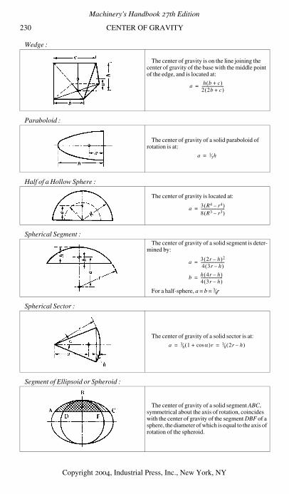
230 CENTER OF GRAVITY
Wedge :
Paraboloid :
Half of a Hollow Sphere :
Spherical Segment :
Spherical Sector :
Segment of Ellipsoid or Spheroid :
The center of gravity is on the line joining the center of gravity of the base with the middle point of the edge, and is located at:
The center of gravity of a solid paraboloid of rotation is at:
The center of gravity is located at:
The center of gravity of a solid segment is deter-mined by:
For a half-sphere, a = b = 3⁄8r
The center of gravity of a solid sector is at:
The center of gravity of a solid segment ABC, symmetrical about the axis of rotation, coincides with the center of gravity of the segment DBF of a sphere, the diameter of which is equal to the axis of rotation of the spheroid.
a h b c+( )
2 2b c+( )-----------------------=
a 1⁄3h=
a 3 R4 r4–( )
8 R3 r3–( )-------------------------=
a 3 2r h–( )2
4 3r h–( )-------------------------=
b h 4r h–( )
4 3r h–( )-----------------------=
a 3⁄8 1 αcos+( )r 3⁄8 2r h–( )= =
Machinery's Handbook 27th Edition
Copyright 2004, Industrial Press, Inc., New York, NY
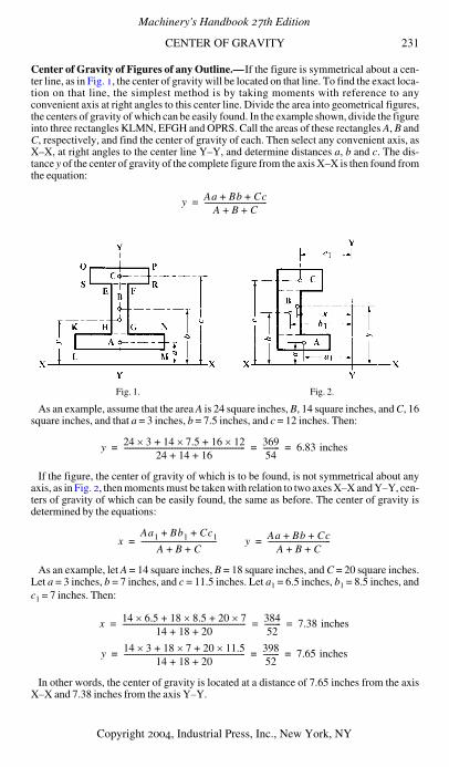
CENTER OF GRAVITY 231
Center of Gravity of Figures of any Outline.—If the figure is symmetrical about a cen-ter line, as in Fig. 1, the center of gravity will be located on that line. To find the exact loca-tion on that line, the simplest method is by taking moments with reference to anyconvenient axis at right angles to this center line. Divide the area into geometrical figures,the centers of gravity of which can be easily found. In the example shown, divide the figureinto three rectangles KLMN, EFGH and OPRS. Call the areas of these rectangles A, B andC, respectively, and find the center of gravity of each. Then select any convenient axis, asX–X, at right angles to the center line Y–Y, and determine distances a, b and c. The dis-tance y of the center of gravity of the complete figure from the axis X–X is then found fromthe equation:
As an example, assume that the area A is 24 square inches, B, 14 square inches, and C, 16square inches, and that a = 3 inches, b = 7.5 inches, and c = 12 inches. Then:
If the figure, the center of gravity of which is to be found, is not symmetrical about anyaxis, as in Fig. 2, then moments must be taken with relation to two axes X–X and Y–Y, cen-ters of gravity of which can be easily found, the same as before. The center of gravity isdetermined by the equations:
As an example, let A = 14 square inches, B = 18 square inches, and C = 20 square inches.Let a = 3 inches, b = 7 inches, and c = 11.5 inches. Let a1 = 6.5 inches, b1 = 8.5 inches, andc1 = 7 inches. Then:
In other words, the center of gravity is located at a distance of 7.65 inches from the axisX–X and 7.38 inches from the axis Y–Y.
Fig. 1. Fig. 2.
y Aa Bb Cc+ +A B C+ +
----------------------------------=
y 24 3× 14+ 7.5× 16+ 12×
24 14 16+ +------------------------------------------------------------------ 369
54--------- 6.83 inches= = =
xAa1 Bb1 Cc1+ +
A B C+ +-----------------------------------------= y Aa Bb Cc+ +
A B C+ +----------------------------------=
x 14 6.5× 18+ 8.5× 20+ 7×
14 18 20+ +------------------------------------------------------------------- 384
52--------- 7.38 inches= = =
y 14 3× 18+ 7× 20+ 11.5×
14 18 20+ +------------------------------------------------------------------ 398
52--------- 7.65 inches= = =
Machinery's Handbook 27th Edition
Copyright 2004, Industrial Press, Inc., New York, NY
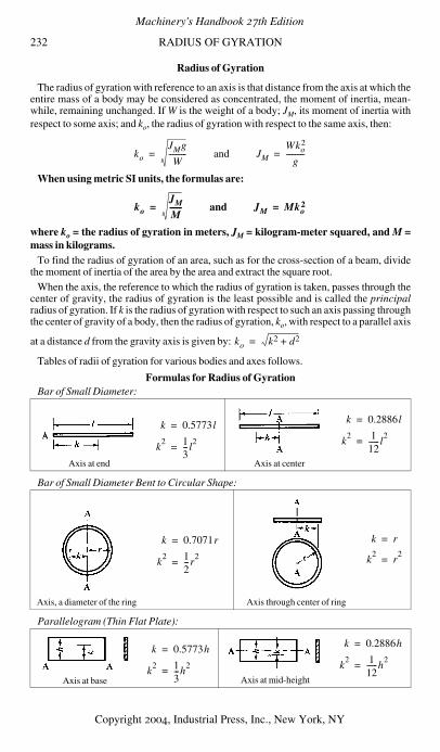
232 RADIUS OF GYRATION
Radius of Gyration
The radius of gyration with reference to an axis is that distance from the axis at which theentire mass of a body may be considered as concentrated, the moment of inertia, mean-while, remaining unchanged. If W is the weight of a body; JM, its moment of inertia withrespect to some axis; and ko, the radius of gyration with respect to the same axis, then:
When using metric SI units, the formulas are:
where ko = the radius of gyration in meters, JM = kilogram-meter squared, and M =mass in kilograms.
To find the radius of gyration of an area, such as for the cross-section of a beam, dividethe moment of inertia of the area by the area and extract the square root.
When the axis, the reference to which the radius of gyration is taken, passes through thecenter of gravity, the radius of gyration is the least possible and is called the principalradius of gyration. If k is the radius of gyration with respect to such an axis passing throughthe center of gravity of a body, then the radius of gyration, ko, with respect to a parallel axis
at a distance d from the gravity axis is given by:
Tables of radii of gyration for various bodies and axes follows.
Formulas for Radius of GyrationBar of Small Diameter:
Bar of Small Diameter Bent to Circular Shape:
Parallelogram (Thin Flat Plate):
Axis at end Axis at center
Axis, a diameter of the ring Axis through center of ring
Axis at base Axis at mid-height
ko
JMg
W----------= and JM
Wko2
g----------=
koJM
M-------= and JM Mko
2=
ko k2 d2+=
k 0.5773l=
k2 1
3--- l
2=
k 0.2886l=
k2 1
12------ l
2=
k 0.7071r=
k2 1
2---r
2=
k r=
k2
r2
=
k 0.5773h=
k2 1
3---h
2=
k 0.2886h=
k2 1
12------h
2=
Machinery's Handbook 27th Edition
Copyright 2004, Industrial Press, Inc., New York, NY
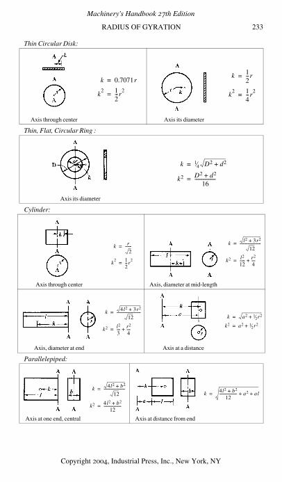
RADIUS OF GYRATION 233
Thin Circular Disk:
Thin, Flat, Circular Ring :
Cylinder:
Parallelepiped:
Axis through center Axis its diameter
Axis its diameter
Axis through center Axis, diameter at mid-length
Axis, diameter at end Axis at a distance
Axis at one end, central Axis at distance from end
k 0.7071r=
k2 1
2---r
2=
k 12---r=
k2 1
4---r
2=
k 1⁄4 D2 d2+=
k2 D2 d2+16
------------------=
k r
2-------=
k2 1
2---r
2=
k l2 3r2+
12-----------------------=
k2 l2
12------ r2
4----+=
k 4l2 3r2+
12--------------------------=
k2 l2
3---- r2
4----+=
k a2 1⁄2r2+=
k2 a2 1⁄2r2+=
k 4l2 b2+
12-----------------------=
k2 4l2 b2+12
-------------------=
k 4l2 b2+12
------------------- a2 al+ +=
Machinery's Handbook 27th Edition
Copyright 2004, Industrial Press, Inc., New York, NY
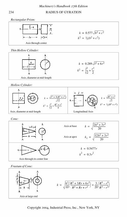
234 RADIUS OF GYRATION
Rectangular Prism:
Thin Hollow Cylinder:
Hollow Cylinder:
Cone:
Frustum of Cone:
Axis through center
Axis, diameter at mid-length
Axis, diameter at mid-length Longitudinal Axis
Axis at base
Axis at apex
Axis through its center line
Axis at large end
k 0.577 b2 c2+=
k2 1⁄3 b2 c2+( )=
k 0.289 l2 6r2+=
k2 l2
12------ r2
2----+=
k l2 3 R2 r2+( )+
12----------------------------------------=
k2 l2
12------ R2 r2+
4-----------------+=
k R2 r2+
2---------------------=
k2 1⁄2 R2 r2+( )=
k 2h2 3r2+20
-----------------------=
k112h2 3r2+
20--------------------------=
k 0.5477r=
k2
0.3r2
=
k h2
10------ R2 3Rr 6r2+ +
R2 Rr r2+ +-------------------------------------⎝ ⎠⎛ ⎞ 3
20------ R5 r5–
R3 r3–-----------------⎝ ⎠⎛ ⎞+=
Machinery's Handbook 27th Edition
Copyright 2004, Industrial Press, Inc., New York, NY
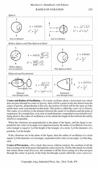
RADIUS OF GYRATION 235
Sphere:
Hollow Sphere and Thin Spherical Shell:
Ellipsoid and Paraboloid:
Center and Radius of Oscillation.—If a body oscillates about a horizontal axis whichdoes not pass through its center of gravity, there will be a point on the line drawn from thecenter of gravity, perpendicular to the axis, the motion of which will be the same as if thewhole mass were concentrated at that point. This point is called the center of oscillation.The radius of oscillation is the distance between the center of oscillation and the point ofsuspension. In a straight line, or in a bar of small diameter, suspended at one end and oscil-lating about it, the center of oscillation is at two-thirds the length of the rod from the end bywhich it is suspended.
When the vibrations are perpendicular to the plane of the figure, and the figure is sus-pended by the vertex of an angle or its uppermost point, the radius of oscillation of an isos-celes triangle is equal to 3⁄4 of the height of the triangle; of a circle, 5⁄8 of the diameter; of aparabola, 5⁄7 of the height.
If the vibrations are in the plane of the figure, then the radius of oscillation of a circleequals 3⁄4 of the diameter; of a rectangle, suspended at the vertex of one angle, 2⁄3 of the diag-onal.
Center of Percussion.—For a body that moves without rotation, the resultant of all theforces acting on the body passes through the center of gravity. On the other hand, for a bodythat rotates about some fixed axis, the resultant of all the forces acting on it does not passthrough the center of gravity of the body but through a point called the center of percus-
Axis its diameter Axis at a distance
Hollow SphereAxis its diameter Thin Spherical Shell
EllipsoidAxis through center
ParaboloidAxis through center
k 0.6325r=
k2 2
5---r
2=
k a2 2⁄5r2+=
k2 a2 2⁄5r2+=
k 0.6325 R5 r5–R3 r3–-----------------=
k2 2 R5 r5–( )5 R3 r3–( )-------------------------=
k 0.8165r=
k2 2
3---r
2=
k b2 c2+
5---------------------=
k2 1⁄5 b2 c2+( )=
k 0.5773r=
k2 1
3---r
2=
Machinery's Handbook 27th Edition
Copyright 2004, Industrial Press, Inc., New York, NY
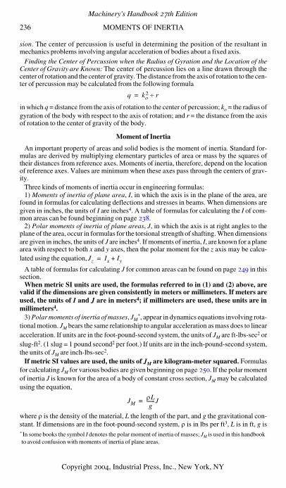
236 MOMENTS OF INERTIA
sion. The center of percussion is useful in determining the position of the resultant inmechanics problems involving angular acceleration of bodies about a fixed axis.
Finding the Center of Percussion when the Radius of Gyration and the Location of theCenter of Gravity are Known: The center of percussion lies on a line drawn through thecenter of rotation and the center of gravity. The distance from the axis of rotation to the cen-ter of percussion may be calculated from the following formula
in which q = distance from the axis of rotation to the center of percussion; ko = the radius ofgyration of the body with respect to the axis of rotation; and r = the distance from the axisof rotation to the center of gravity of the body.
Moment of Inertia
An important property of areas and solid bodies is the moment of inertia. Standard for-mulas are derived by multiplying elementary particles of area or mass by the squares oftheir distances from reference axes. Moments of inertia, therefore, depend on the locationof reference axes. Values are minimum when these axes pass through the centers of grav-ity.
Three kinds of moments of inertia occur in engineering formulas:1) Moments of inertia of plane area, I, in which the axis is in the plane of the area, are
found in formulas for calculating deflections and stresses in beams. When dimensions aregiven in inches, the units of I are inches4. A table of formulas for calculating the I of com-mon areas can be found beginning on page 238.
2) Polar moments of inertia of plane areas, J, in which the axis is at right angles to theplane of the area, occur in formulas for the torsional strength of shafting. When dimensionsare given in inches, the units of J are inches4. If moments of inertia, I, are known for a planearea with respect to both x and y axes, then the polar moment for the z axis may be calcu-lated using the equation,
A table of formulas for calculating J for common areas can be found on page 249 in thissection.
When metric SI units are used, the formulas referred to in (1) and (2) above, arevalid if the dimensions are given consistently in meters or millimeters. If meters areused, the units of I and J are in meters4; if millimeters are used, these units are inmillimeters4.
3) Polar moments of inertia of masses, JM*, appear in dynamics equations involving rota-
tional motion. JM bears the same relationship to angular acceleration as mass does to linearacceleration. If units are in the foot-pound-second system, the units of JM are ft-lbs-sec2 orslug-ft2. (1 slug = 1 pound second2 per foot.) If units are in the inch-pound-second system,the units of JM are inch-lbs-sec2.
If metric SI values are used, the units of JM are kilogram-meter squared. Formulasfor calculating JM for various bodies are given beginning on page 250. If the polar momentof inertia J is known for the area of a body of constant cross section, JM may be calculatedusing the equation,
where ρ is the density of the material, L the length of the part, and g the gravitational con-stant. If dimensions are in the foot-pound-second system, ρ is in lbs per ft3, L is in ft, g is* In some books the symbol I denotes the polar moment of inertia of masses; JM is used in this handbookto avoid confusion with moments of inertia of plane areas.
q ko2 r÷=
Jz Ix Iy+=
JMρLg
-------J=
Machinery's Handbook 27th Edition
Copyright 2004, Industrial Press, Inc., New York, NY
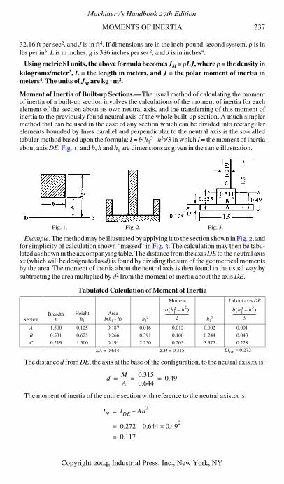
MOMENTS OF INERTIA 237
32.16 ft per sec2, and J is in ft4. If dimensions are in the inch-pound-second system, ρ is inlbs per in3, L is in inches, g is 386 inches per sec2, and J is in inches4.
Using metric SI units, the above formula becomes JM = ρLJ, where ρ = the density inkilograms/meter3, L = the length in meters, and J = the polar moment of inertia inmeters4. The units of JM are kg · m2.
Moment of Inertia of Built-up Sections.—The usual method of calculating the momentof inertia of a built-up section involves the calculations of the moment of inertia for eachelement of the section about its own neutral axis, and the transferring of this moment ofinertia to the previously found neutral axis of the whole built-up section. A much simplermethod that can be used in the case of any section which can be divided into rectangularelements bounded by lines parallel and perpendicular to the neutral axis is the so-calledtabular method based upon the formula: I = b(h1
3 - h3)/3 in which I = the moment of inertiaabout axis DE, Fig. 1, and b, h and h1 are dimensions as given in the same illustration.
Example:The method may be illustrated by applying it to the section shown in Fig. 2, andfor simplicity of calculation shown “massed” in Fig. 3. The calculation may then be tabu-lated as shown in the accompanying table. The distance from the axis DE to the neutral axisxx (which will be designated as d) is found by dividing the sum of the geometrical momentsby the area. The moment of inertia about the neutral axis is then found in the usual way bysubtracting the area multiplied by d2 from the moment of inertia about the axis DE.
Tabulated Calculation of Moment of Inertia
The distance d from DE, the axis at the base of the configuration, to the neutral axis xx is:
The moment of inertia of the entire section with reference to the neutral axis xx is:
Fig. 1. Fig. 2. Fig. 3.
SectionBreadth
bHeight
h1
Areab(h1 - h) h1
2
Moment
h13
I about axis DE
A 1.500 0.125 0.187 0.016 0.012 0.002 0.001
B 0.531 0.625 0.266 0.391 0.100 0.244 0.043
C 0.219 1.500 0.191 2.250 0.203 3.375 0.228
ΣA = 0.644 ΣM = 0.315 ΣIDE = 0.272
b h12 h
2–( )
2-------------------------
b h13 h
3–( )
3-------------------------
d MA----- 0.315
0.644------------- 0.49= = =
IN IDE Ad2
–=
0.272 0.644 0.492
×–=
0.117=
Machinery's Handbook 27th Edition
Copyright 2004, Industrial Press, Inc., New York, NY
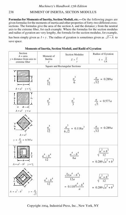
238 MOMENT OF INERTIA, SECTION MODULUS
Formulas for Moments of Inertia, Section Moduli, etc.—On the following pages aregiven formulas for the moments of inertia and other properties of forty-two different cross-sections. The formulas give the area of the section A, and the distance y from the neutralaxis to the extreme fiber, for each example. Where the formulas for the section modulusand radius of gyration are very lengthy, the formula for the section modulus, for example,
has been simply given as . The radius of gyration is sometimes given as tosave space.
Moments of Inertia, Section Moduli, and Radii of Gyration
SectionA = area
y = distance from axis to extreme fiber
Moment ofInertia
I
Section Modulus Radius of Gyration
Square and Rectangular Sections
A = a2 y = a⁄2
A = a2 y = a
A = a2
A = a2 − b2 y = a⁄2
I y÷ I A÷
Z Iy--= k I
A---=
a4
12------
a3
6-----
a
12---------- 0.289a=
a4
3----- a
3
3-----
a
3------- 0.577a=
y a
2------- 0.707a= =
a4
12------
a3
6 2---------- 0.118a
3=
a
12---------- 0.289a=
a4
b4
–12
-----------------a
4b
4–
6a-----------------
a2
b2
+12
-----------------
0.289 a2
b2
+=
A a2
b2
–= y a
2-------=
a4
b4
–12
-----------------
2 a4
b4
–( )
12a-----------------------------
0.118a4
b4
–a
-----------------=
a2
b2
+12
-----------------
0.289 a2
b2
+=
Machinery's Handbook 27th Edition
Copyright 2004, Industrial Press, Inc., New York, NY
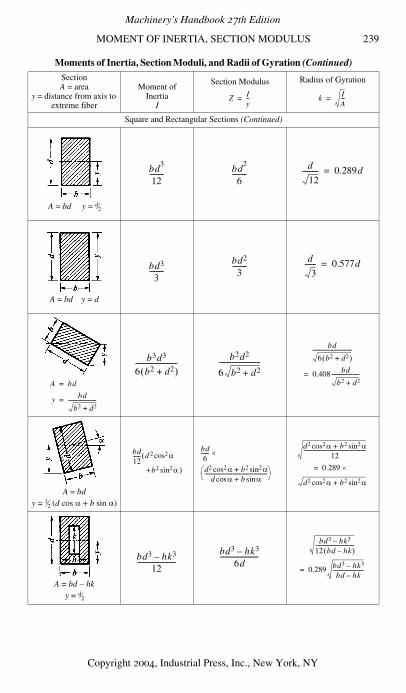
MOMENT OF INERTIA, SECTION MODULUS 239
A = bd y = d⁄2
A = bd y = d
A = bdy = 1⁄2 (d cos α + b sin α)
A = bd − hky = d⁄2
Moments of Inertia, Section Moduli, and Radii of Gyration (Continued)
SectionA = area
y = distance from axis to extreme fiber
Moment ofInertia
I
Section Modulus Radius of Gyration
Square and Rectangular Sections (Continued)
Z Iy--= k I
A---=
bd3
12--------- bd
2
6---------
d
12---------- 0.289d=
bd3
3---------
bd2
3---------
d
3------- 0.577d=
A bd=
y bd
b2 d2+---------------------=
b3d3
6 b2 d2+( )-------------------------
b2d2
6 b2 d2+-------------------------
bd
6 b2 d2+( )------------------------------
0.408 bd
b2 d2+---------------------=
bd12------ d( 2 αcos2
+b2 αsin2 )
bd6
------
d2 αcos2 b2 αsin2+d αcos b αsin+
-----------------------------------------------⎝ ⎠⎛ ⎞
×d2 αcos2 b2 αsin2+
12-----------------------------------------------
0.289 ×=
d2 αcos2 b2 αsin2+
bd3 hk3–12
-----------------------bd3 hk3–
6d-----------------------
bd3 hk3–12 bd hk–( )-----------------------------
0.289 bd3 hk3–bd hk–
-----------------------=
Machinery's Handbook 27th Edition
Copyright 2004, Industrial Press, Inc., New York, NY
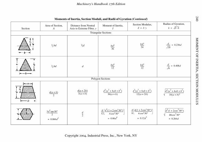
MO
ME
NT
OF IN
ER
TIA
, SEC
TIO
N M
OD
UL
US
240 Moments of Inertia, Section Moduli, and Radii of Gyration (Continued)
SectionArea of Section,
ADistance from Neutral
Axis to Extreme Fiber, yMoment of Inertia,
I
Section Modulus, Radius of Gyration,
Triangular Sections
1⁄2 bd 2⁄3d
1⁄2 bd d
Polygon Sections
Z I y⁄= k I A⁄=
bd3
36---------
bd2
24---------
d
18---------- 0.236d=
bd3
12--------- bd2
12---------
d
6------- 0.408d=
d a b+( )
2--------------------
d a 2b+( )
3 a b+( )------------------------ d
3a
24ab b
2+ +( )
36 a b+( )--------------------------------------------
d2
a2
4ab b2
+ +( )
12 a 2b+( )-------------------------------------------- d
2a
24ab b
2+ +( )
18 a b+( )2--------------------------------------------
3d2
30tan °
2--------------------------
0.866d2
=
d2---
A12------ d
21 2 30cos2 °+( )
4 30cos2 °-------------------------------------------
0.06d4
=
A6--- d 1 2 30cos2 °+( )
4 30cos2 °-----------------------------------------
0.12d3
=
d2
1 2cos230°+( )
48cos230°
-------------------------------------------
0.264d=
Machinery's Handbook 27th Edition
Copyright 2004, Industrial Press, Inc., New York, NY
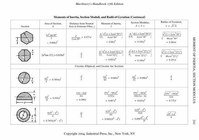
MO
ME
NT
OF IN
ER
TIA
, SEC
TIO
N M
OD
UL
US
241
2d2tan 221⁄2 = 0.828d2
Circular, Elliptical, and Circular Arc Sections
Moments of Inertia, Section Moduli, and Radii of Gyration (Continued)
SectionArea of Section,
ADistance from Neutral
Axis to Extreme Fiber, yMoment of Inertia,
I
Section Modulus, Radius of Gyration,
Z I y⁄= k I A⁄=
3d2
30tan °
2--------------------------
0.866d2
=
d2 30cos °--------------------- 0.577d=
A12------ d
21 2 30cos2 °+( )
4 30cos2 °-------------------------------------------
0.06d4
=
A6.9------- d 1 2 30cos2 °+( )
4 30cos2 °-----------------------------------------
0.104d3
=
d2
1 2cos230°+( )
48cos230°
-------------------------------------------
0.264d=
d2---
A12------ d
21 2 221⁄2
°cos2+( )
4 221⁄2°cos2
-----------------------------------------------
0.055d4
=
A6---
d 1 2cos2221⁄2°+( )
4cos2221⁄2°
---------------------------------------------
0.109d3
=
d2
1 2cos2221⁄2°+( )
48cos2221⁄2°
------------------------------------------------
0.257d=
πd2
4--------- 0.7854d
2=
d2--- πd
4
64--------- 0.049d
4= πd
3
32--------- 0.098d
3=
d4---
πd2
8--------- 0.393d
2=
3π 4–( )d6π
------------------------
0.288d=
9π2
64–( )d4
1152π--------------------------------
0.007d4
=
9π2
64–( )d3
192 3π 4–( )--------------------------------
0.024d3
=
9π2
64–( )d2
12π------------------------------------
0.132d=
π D2
d2
–( )
4--------------------------
0.7854 D2
d2
–( )=
D2----
π D4
d4
–( )
64--------------------------
0.049 D4
d4
–( )=
π D4
d4
–( )
32D--------------------------
0.098D4
d4
–D
------------------=
D2
d2
+4
----------------------
Machinery's Handbook 27th Edition
Copyright 2004, Industrial Press, Inc., New York, NY
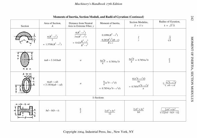
MO
ME
NT
OF IN
ER
TIA
, SEC
TIO
N M
OD
UL
US
242
πab = 3.1416ab a
π(ab − cd) = 3.1416(ab − cd)
a
I–Sections
bd − h(b − t)
Moments of Inertia, Section Moduli, and Radii of Gyration (Continued)
SectionArea of Section,
ADistance from Neutral
Axis to Extreme Fiber, yMoment of Inertia,
I
Section Modulus, Radius of Gyration,
Z I y⁄= k I A⁄=
π R2
r2
–( )
2-------------------------
1.5708 R2
r2
–( )=
4 R3
r3
–( )
3π R2
r2
–( )-----------------------------
0.424R3
r3
–
R2
r2
–----------------=
0.1098 R4
r4
–( )
0.283R2r
2R r–( )
R r+------------------------------------------–
Iy-- I
A---
πa3b4
------------ 0.7854a3b=πa2b
4------------ 0.7854a2b= a
2---
π
4--- a3b c3d–( )
0.7854= a3b c3d–( )
π a3b c3d–( )
4a--------------------------------
0.7854a3b c3d–a
-----------------------=
1⁄2a3b c3d–ab cd–
-----------------------
b2--- 2sb3 ht3+
12-------------------------
2sb3 ht3+6b
------------------------- 2sb3 ht3+12 bd h b t–( )–[ ]------------------------------------------
Machinery's Handbook 27th Edition
Copyright 2004, Industrial Press, Inc., New York, NY
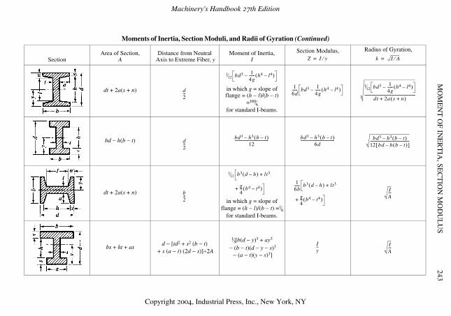
MO
ME
NT
OF IN
ER
TIA
, SEC
TIO
N M
OD
UL
US
243
dt + 2a(s + n) in which g = slope offlange = (h − l)/(b − t)
=10.0⁄6for standard I-beams.
bd − h(b − t)
dt + 2a(s + n)
in which g = slope offlange = (h − l)/(b − t) =1⁄6
for standard I-beams.
bs + ht + asd − [td2 + s2 (b − t)
+ s (a − t) (2d − s)]÷2A
1⁄3[b(d − y)3 + ay3 − (b − t)(d − y − s)3
− (a − t)(y − s)3]
Moments of Inertia, Section Moduli, and Radii of Gyration (Continued)
SectionArea of Section,
ADistance from Neutral
Axis to Extreme Fiber, yMoment of Inertia,
I
Section Modulus, Radius of Gyration,
Z I y⁄= k I A⁄=
d2---
1⁄12 bd3 14g------ h4 l4–( )–
16d------ bd3 1
4g------ h4 l4–( )–
1⁄12 bd3 14g------ h4 l4–( )–
dt 2a s n+( )+-------------------------------------------------------
d2---
bd3 h3 b t–( )–12
------------------------------------ bd3 h3 b t–( )–6d
------------------------------------ bd3 h3 b t–( )–12 bd h b t–( )–[ ]------------------------------------------
b2---
1⁄12 b3 d h–( ) lt3
g4--- b4 t4–( )
+
+1
6b------ b3 d h–( ) lt3
g4--- b4 t4–( )
+
+
IA---
Iy-- I
A---
Machinery's Handbook 27th Edition
Copyright 2004, Industrial Press, Inc., New York, NY
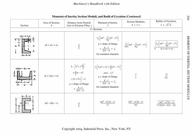
MO
ME
NT
OF IN
ER
TIA
, SEC
TIO
N M
OD
UL
US
244
C–Sections
dt + a(s + n) g = slope of flange
for standard channels.
dt + 2a(s + n)
g = slope of flange
g = slope of flange
for standard channels.
bd − h(b − t)
Moments of Inertia, Section Moduli, and Radii of Gyration (Continued)
SectionArea of Section,
ADistance from Neutral
Axis to Extreme Fiber, yMoment of Inertia,
I
Section Modulus, Radius of Gyration,
Z I y⁄= k I A⁄=
d2---
1⁄12 bd3 18g------ h4 l4–( )–
h l–2 b t–( )------------------= 1⁄6=
16d------ bd3 1
8g------ h4 l4–( )–
1⁄12 bd3 18g------ h4 l4–( )–
dt a s n+( )+-------------------------------------------------------
b b2s ht
2
2-------
g3--- b t–( )2
b 2t+( )×
+
+
A÷
–
h l–2 b t–( )------------------=
1⁄3 2sb3 lt3 g2--- b4 t4–( )+ +
A b y–( )2–
h l–2 b t–( )------------------= 1⁄6=
Iy-- I
A---
d2---
bd3 h3 b t–( )–12
------------------------------------ bd3 h3 b t–( )–6d
------------------------------------ bd3 h3 b t–( )–12 bd h b t–( )–[ ]------------------------------------------
Machinery's Handbook 27th Edition
Copyright 2004, Industrial Press, Inc., New York, NY
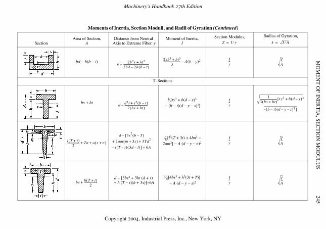
MO
ME
NT
OF IN
ER
TIA
, SEC
TIO
N M
OD
UL
US
245
bd − h(b − t)
T–Sections
bs + ht1⁄3[ty3 + b(d − y)3
− (b − t)(d − y − s)3]
1⁄12[l3(T + 3t) + 4bn3 − 2am3] − A (d − y − n)2
d − [3bs2 + 3ht (d + s) + h (T − t)(h + 3s)]÷6A
1⁄12[4bs3 + h3(3t + T)] − A (d − y − s)2
Moments of Inertia, Section Moduli, and Radii of Gyration (Continued)
SectionArea of Section,
ADistance from Neutral
Axis to Extreme Fiber, yMoment of Inertia,
I
Section Modulus, Radius of Gyration,
Z I y⁄= k I A⁄=
b 2b2s ht2+2bd 2h b t–( )–--------------------------------------–
2sb3 ht3+3
------------------------- A b y–( )2– Iy-- I
A---
d d2t s2 b t–( )+2 bs ht+( )
----------------------------------–Iy--
13 bs ht+( )------------------------- t[ y3 b d y–( )3+
b t–( ) d y– s–( )3 ]–
l T t+( )
2------------------ Tn a s n+( )+ +
d 3s2
b T–( )
2am m 3s+( ) 3Td2
l T t–( ) 3d l–( )–
+ +
[
] 6A÷
–Iy-- I
A---
bs h T t+( )
2-------------------+
Iy-- I
A---
Machinery's Handbook 27th Edition
Copyright 2004, Industrial Press, Inc., New York, NY
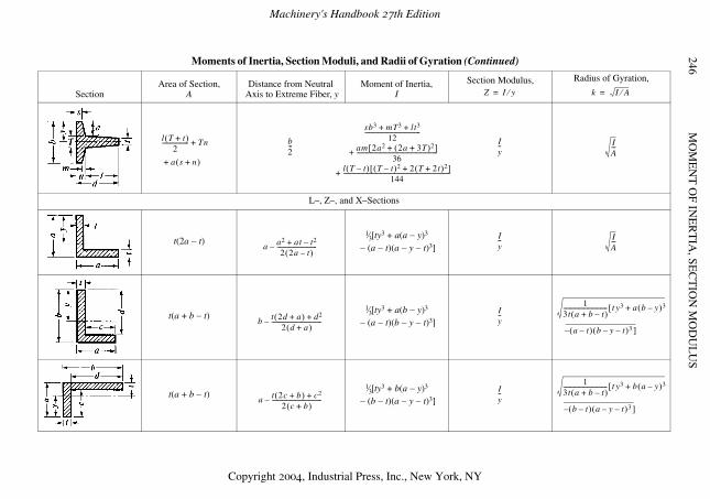
MO
ME
NT
OF IN
ER
TIA
, SEC
TIO
N M
OD
UL
US
246
L–, Z–, and X–Sections
t(2a − t)1⁄3[ty3 + a(a − y)3
− (a − t)(a − y − t)3]
t(a + b − t)1⁄3[ty3 + a(b − y)3
− (a − t)(b − y − t)3]
t(a + b − t)1⁄3[ty3 + b(a − y)3
− (b − t)(a − y − t)3]
Moments of Inertia, Section Moduli, and Radii of Gyration (Continued)
SectionArea of Section,
ADistance from Neutral
Axis to Extreme Fiber, yMoment of Inertia,
I
Section Modulus, Radius of Gyration,
Z I y⁄= k I A⁄=
l T t+( )
2------------------ Tn
a s n+( )
+
+
b2---
sb3 mT3 lt3+ +12
--------------------------------------
am 2a2 2a 3T+( )2+[ ]
36-------------------------------------------------------
l T t–( ) T t–( )2 2 T 2t+( )2+[ ]
144-------------------------------------------------------------------------
+
+
Iy-- I
A---
a a2 at t2–+2 2a t–( )
---------------------------–Iy-- I
A---
b t 2d a+( ) d2+2 d a+( )
----------------------------------–Iy--
13t a b t–+( )------------------------------ t[ y3 a b y–( )3+
a t–( ) b y– t–( )3 ]–
a t 2c b+( ) c2+2 c b+( )
----------------------------------–Iy--
13t a b t–+( )------------------------------ t[ y3 b a y–( )3+
b t–( ) a y– t–( )3 ]–
Machinery's Handbook 27th Edition
Copyright 2004, Industrial Press, Inc., New York, NY
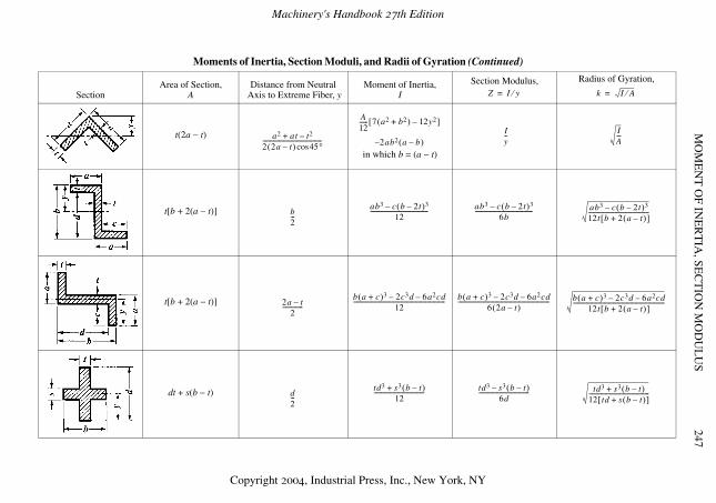
MO
ME
NT
OF IN
ER
TIA
, SEC
TIO
N M
OD
UL
US
247
t(2a − t)
in which b = (a − t)
t[b + 2(a − t)]
t[b + 2(a − t)]
dt + s(b − t)
Moments of Inertia, Section Moduli, and Radii of Gyration (Continued)
SectionArea of Section,
ADistance from Neutral
Axis to Extreme Fiber, yMoment of Inertia,
I
Section Modulus, Radius of Gyration,
Z I y⁄= k I A⁄=
a2 at t2–+2 2a t–( ) 45°cos----------------------------------------
A12------ 7 a2 b2+( ) 12y2–[ ]
2ab2 a b–( )–Iy-- I
A---
b2---
ab3 c b 2t–( )3–12
--------------------------------------- ab3 c b 2t–( )3–6b
--------------------------------------- ab3 c b 2t–( )3–12t b 2 a t–( )+[ ]-----------------------------------------
2a t–2
--------------b a c+( )3 2c3d– 6a2cd–
12-------------------------------------------------------------- b a c+( )3 2c3d– 6a2cd–
6 2a t–( )-------------------------------------------------------------- b a c+( )3 2c3d– 6a2cd–
12t b 2 a t–( )+[ ]--------------------------------------------------------------
d2---
td3 s3 b t–( )+12
---------------------------------- td3 s3 b t–( )–6d
---------------------------------- td3 s3 b t–( )+12 td s b t–( )+[ ]-----------------------------------------
Machinery's Handbook 27th Edition
Copyright 2004, Industrial Press, Inc., New York, NY
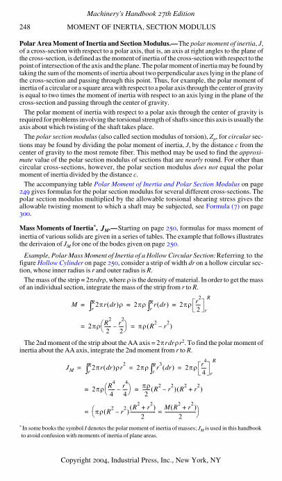
248 MOMENT OF INERTIA, SECTION MODULUS
Polar Area Moment of Inertia and Section Modulus.—The polar moment of inertia, J,of a cross-section with respect to a polar axis, that is, an axis at right angles to the plane ofthe cross-section, is defined as the moment of inertia of the cross-section with respect to thepoint of intersection of the axis and the plane. The polar moment of inertia may be found bytaking the sum of the moments of inertia about two perpendicular axes lying in the plane ofthe cross-section and passing through this point. Thus, for example, the polar moment ofinertia of a circular or a square area with respect to a polar axis through the center of gravityis equal to two times the moment of inertia with respect to an axis lying in the plane of thecross-section and passing through the center of gravity.
The polar moment of inertia with respect to a polar axis through the center of gravity isrequired for problems involving the torsional strength of shafts since this axis is usually theaxis about which twisting of the shaft takes place.
The polar section modulus (also called section modulus of torsion), Zp, for circular sec-tions may be found by dividing the polar moment of inertia, J, by the distance c from thecenter of gravity to the most remote fiber. This method may be used to find the approxi-mate value of the polar section modulus of sections that are nearly round. For other thancircular cross-sections, however, the polar section modulus does not equal the polarmoment of inertia divided by the distance c.
The accompanying table Polar Moment of Inertia and Polar Section Modulus on page249 gives formulas for the polar section modulus for several different cross-sections. Thepolar section modulus multiplied by the allowable torsional shearing stress gives theallowable twisting moment to which a shaft may be subjected, see Formula (7) on page300.
Mass Moments of Inertia*, JM.—Starting on page 250, formulas for mass moment ofinertia of various solids are given in a series of tables. The example that follows illustratesthe derivaion of JM for one of the bodes given on page 250.
Example, Polar Mass Moment of Inertia of a Hollow Circular Section:Referring to thefigure Hollow Cylinder on page 250, consider a strip of width dr on a hollow circular sec-tion, whose inner radius is r and outer radius is R.
The mass of the strip = 2πrdrρ, where ρ is the density of material. In order to get the massof an individual section, integrate the mass of the strip from r to R.
The 2nd moment of the strip about the AA axis = 2πrdrρr2. To find the polar moment ofinertia about the AA axis, integrate the 2nd moment from r to R.
* In some books the symbol I denotes the polar moment of inertia of masses; JM is used in this handbookto avoid confusion with moments of inertia of plane areas.
M 2πr rd( )ρrR∫ 2πρ r rd( )
rR∫ 2πρ r
2
2----
r
R
= = =
2πρ R2
2------ r
2
2----–⎝ ⎠
⎛ ⎞= πρ R2
r2
–( )=
JM 2πr rd( )ρr2
rR∫ 2πρ r
3rd( )
rR∫ 2πρ r
4
4----
r
R
= = =
2πρ R4
4------ r
4
4----–⎝ ⎠
⎛ ⎞= πρ2
------- R2
r2
–( ) R2
r2
+( )=
πρ R2
r2
–( )R
2r
2+( )2
----------------------M R
2r
2+( )
2---------------------------=⎝ ⎠
⎛ ⎞=
Machinery's Handbook 27th Edition
Copyright 2004, Industrial Press, Inc., New York, NY
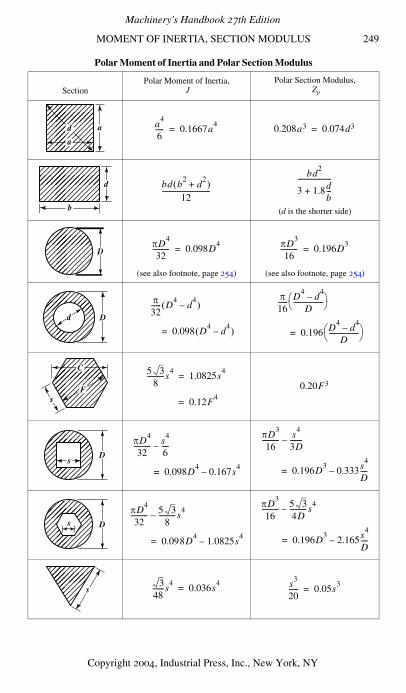
MOMENT OF INERTIA, SECTION MODULUS 249
Polar Moment of Inertia and Polar Section Modulus
SectionPolar Moment of Inertia,
JPolar Section Modulus,
Zp
(d is the shorter side)
(see also footnote, page 254) (see also footnote, page 254)
����
ad
a
a4
6----- 0.1667a
4= 0.208a3 0.074d3=
����
d
b
bd b2
d2
+( )12
-----------------------------
bd2
3 1.8db---+
--------------------����
DπD
4
32---------- 0.098D
4= πD
3
16---------- 0.196D
3=��
��d D
π32------ D
4d
4–( )
0.098 D4
d4
–( )=
π16------ D
4d
4–D
------------------⎝ ⎠⎛ ⎞
0.196 D4
d4
–D
------------------⎝ ⎠⎛ ⎞=
����C
sF
5 38
----------s4
1.0825s4
=
0.12F4
=
0.20F3����
Ds
πD4
32---------- s
4
6----–
0.098D4
0.167s4
–=
πD3
16---------- s
4
3D-------–
0.196D3
0.333s4
D----–=
����
Ds
πD4
32---------- 5 3
8----------s
4–
0.098D4
1.0825s4
–=
πD3
16---------- 5 3
4D----------s
4–
0.196D3
2.165s4
D----–=
����
s3
48-------s
40.036s
4= s
3
20------ 0.05s
3=
Machinery's Handbook 27th Edition
Copyright 2004, Industrial Press, Inc., New York, NY

250 POLAR MOMENTS OF INERTIA
Formulas for Polar Moment of Inertia of Masses, JM
Prism:
Cylinder:
Hollow Cylinder:
Pyramid, Rectangular Base:
Sphere:
With reference to axis A − A:
With reference to axis B − B:
With reference to axis A − A:
With reference to axis B − B:
With reference to axis A − A:
With reference to axis B − B:
With reference to axis A − A:
With reference to axis B − B (through the center of grav-ity):
With reference to any axis through the center:
JMM12------ h2 b2+( )=
JM M l2
3---- h2
12------+⎝ ⎠
⎛ ⎞=
JM1⁄2Mr2=
JM M l2
3---- r2
4----+⎝ ⎠
⎛ ⎞=
JM1⁄2M R2 r2+( )=
JM M l2
3---- R2 r2+
4-----------------+⎝ ⎠
⎛ ⎞=
JMM20------ a2 b2+( )=
JM M 380------h2 b2
20------+⎝ ⎠
⎛ ⎞=
JM2⁄5Mr2=
Machinery's Handbook 27th Edition
Copyright 2004, Industrial Press, Inc., New York, NY
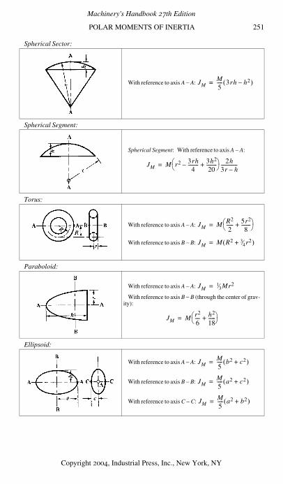
POLAR MOMENTS OF INERTIA 251
Spherical Sector:
Spherical Segment:
Torus:
Paraboloid:
Ellipsoid:
With reference to axis A − A:
Spherical Segment: With reference to axis A − A:
With reference to axis A − A:
With reference to axis B − B:
With reference to axis A − A:
With reference to axis B − B (through the center of grav-ity):
With reference to axis A − A:
With reference to axis B − B:
With reference to axis C − C:
JMM5----- 3rh h2–( )=
JM M r2 3rh4
---------– 3h2
20---------+⎝ ⎠
⎛ ⎞ 2h3r h–--------------=
JM M R2
2------ 5r2
8--------+⎝ ⎠
⎛ ⎞=
JM M R2 3⁄4r2+( )=
JM1⁄3Mr2=
JM M r2
6---- h2
18------+⎝ ⎠
⎛ ⎞=
JMM5----- b2 c2+( )=
JMM5----- a2 c2+( )=
JMM5----- a2 b2+( )=
Machinery's Handbook 27th Edition
Copyright 2004, Industrial Press, Inc., New York, NY
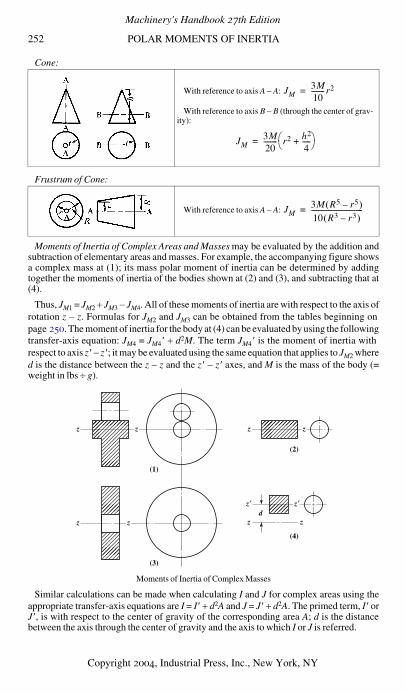
252 POLAR MOMENTS OF INERTIA
Cone:
Frustrum of Cone:
Moments of Inertia of Complex Areas and Masses may be evaluated by the addition andsubtraction of elementary areas and masses. For example, the accompanying figure showsa complex mass at (1); its mass polar moment of inertia can be determined by addingtogether the moments of inertia of the bodies shown at (2) and (3), and subtracting that at(4).
Thus, JM1 = JM2 + JM3 − JM4. All of these moments of inertia are with respect to the axis ofrotation z − z. Formulas for JM2 and JM3 can be obtained from the tables beginning onpage 250. The moment of inertia for the body at (4) can be evaluated by using the followingtransfer-axis equation: JM4 = JM4 ′ + d2M. The term JM4 ′ is the moment of inertia withrespect to axis z ′ − z ′; it may be evaluated using the same equation that applies to JM2 whered is the distance between the z − z and the z ′ − z ′ axes, and M is the mass of the body (=weight in lbs ÷ g).
Moments of Inertia of Complex Masses
Similar calculations can be made when calculating I and J for complex areas using theappropriate transfer-axis equations are I = I ′ + d2A and J = J ′ + d2A. The primed term, I ′ orJ ′, is with respect to the center of gravity of the corresponding area A; d is the distancebetween the axis through the center of gravity and the axis to which I or J is referred.
With reference to axis A − A:
With reference to axis B − B (through the center of grav-ity):
With reference to axis A − A:
JM3M10--------r2=
JM3M20-------- r2 h2
4-----+⎝ ⎠
⎛ ⎞=
JM3M R5 r5–( )10 R3 r3–( )-------------------------------=
���
d
������
����
z
zz
zz z
��z′z′
zz
(2)
(4)
(1)
(3)
��
Machinery's Handbook 27th Edition
Copyright 2004, Industrial Press, Inc., New York, NY
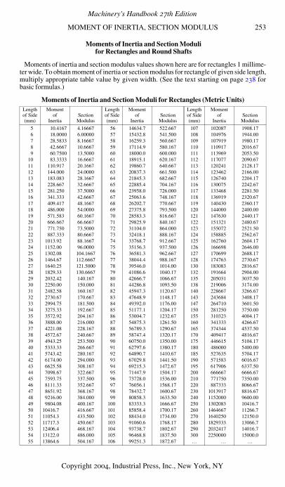
MOMENT OF INERTIA, SECTION MODULUS 253
Moments of Inertia and Section Moduli for Rectangles and Round Shafts
Moments of inertia and section modulus values shown here are for rectangles 1 millime-ter wide. To obtain moment of inertia or section modulus for rectangle of given side length,multiply appropriate table value by given width. (See the text starting on page 238 forbasic formulas.)
Moments of Inertia and Section Moduli for Rectangles (Metric Units)Lengthof Side(mm)
Momentof
InertiaSection
Modulus
Lengthof Side(mm)
Momentof
InertiaSection
Modulus
Lengthof Side(mm)
Momentof
InertiaSection
Modulus
5 10.4167 4.16667 56 14634.7 522.667 107 102087 1908.176 18.0000 6.00000 57 15432.8 541.500 108 104976 1944.007 28.5833 8.16667 58 16259.3 560.667 109 107919 1980.178 42.6667 10.6667 59 17114.9 580.167 110 110917 2016.679 60.7500 13.5000 60 18000.0 600.000 111 113969 2053.50
10 83.3333 16.6667 61 18915.1 620.167 112 117077 2090.6711 110.917 20.1667 62 19860.7 640.667 113 120241 2128.1712 144.000 24.0000 63 20837.3 661.500 114 123462 2166.0013 183.083 28.1667 64 21845.3 682.667 115 126740 2204.1714 228.667 32.6667 65 22885.4 704.167 116 130075 2242.6715 281.250 37.5000 66 23958.0 726.000 117 133468 2281.5016 341.333 42.6667 67 25063.6 748.167 118 136919 2320.6717 409.417 48.1667 68 26202.7 770.667 119 140430 2360.1718 486.000 54.0000 69 27375.8 793.500 120 144000 2400.0019 571.583 60.1667 70 28583.3 816.667 121 147630 2440.1720 666.667 66.6667 71 29825.9 840.167 122 151321 2480.6721 771.750 73.5000 72 31104.0 864.000 123 155072 2521.5022 887.333 80.6667 73 32418.1 888.167 124 158885 2562.6723 1013.92 88.1667 74 33768.7 912.667 125 162760 2604.1724 1152.00 96.0000 75 35156.3 937.500 126 166698 2646.0025 1302.08 104.1667 76 36581.3 962.667 127 170699 2688.1726 1464.67 112.6667 77 38044.4 988.167 128 174763 2730.6727 1640.25 121.5000 78 39546.0 1014.00 130 183083 2816.6728 1829.33 130.6667 79 41086.6 1040.17 132 191664 2904.0029 2032.42 140.167 80 42666.7 1066.67 135 205031 3037.5030 2250.00 150.000 81 44286.8 1093.50 138 219006 3174.0031 2482.58 160.167 82 45947.3 1120.67 140 228667 3266.6732 2730.67 170.667 83 47648.9 1148.17 143 243684 3408.1733 2994.75 181.500 84 49392.0 1176.00 147 264710 3601.5034 3275.33 192.667 85 51177.1 1204.17 150 281250 3750.0035 3572.92 204.167 86 53004.7 1232.67 155 310323 4004.1736 3888.00 216.000 87 54875.3 1261.50 160 341333 4266.6737 4221.08 228.167 88 56789.3 1290.67 165 374344 4537.5038 4572.67 240.667 89 58747.4 1320.17 170 409417 4816.6739 4943.25 253.500 90 60750.0 1350.00 175 446615 5104.1740 5333.33 266.667 91 62797.6 1380.17 180 486000 5400.0041 5743.42 280.167 92 64890.7 1410.67 185 527635 5704.1742 6174.00 294.000 93 67029.8 1441.50 190 571583 6016.6743 6625.58 308.167 94 69215.3 1472.67 195 617906 6337.5044 7098.67 322.667 95 71447.9 1504.17 200 666667 6666.6745 7593.75 337.500 96 73728.0 1536.00 210 771750 7350.0046 8111.33 352.667 97 76056.1 1568.17 220 887333 8066.6747 8651.92 368.167 98 78432.7 1600.67 230 1013917 8816.6748 9216.00 384.000 99 80858.3 1633.50 240 1152000 9600.0049 9804.08 400.167 100 83333.3 1666.67 250 1302083 10416.750 10416.7 416.667 101 85858.4 1700.17 260 1464667 11266.751 11054.3 433.500 102 88434.0 1734.00 270 1640250 12150.052 11717.3 450.667 103 91060.6 1768.17 280 1829333 13066.753 12406.4 468.167 104 93738.7 1802.67 290 2032417 14016.754 13122.0 486.000 105 96468.8 1837.50 300 2250000 15000.055 13864.6 504.167 106 99251.3 1872.67 … … …
Machinery's Handbook 27th Edition
Copyright 2004, Industrial Press, Inc., New York, NY
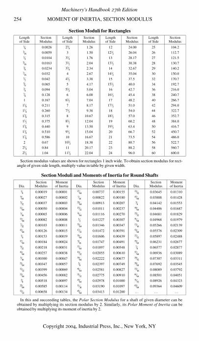
254 MOMENT OF INERTIA, SECTION MODULUS
Section Moduli for Rectangles
Section modulus values are shown for rectangles 1 inch wide. To obtain section modulus for rect-angle of given side length, multiply value in table by given width.
Section Moduli and Moments of Inertia for Round Shafts
In this and succeeding tables, the Polar Section Modulus for a shaft of given diameter can beobtained by multiplying its section modulus by 2. Similarly, its Polar Moment of Inertia can beobtained by multiplying its moment of inertia by 2.
Length of Side
SectionModulus
Length of Side
SectionModulus
Length of Side
SectionModulus
Length of Side
SectionModulus
1⁄8 0.0026 23⁄4 1.26 12 24.00 25 104.23⁄16 0.0059 3 1.50 121⁄2 26.04 26 112.71⁄4 0.0104 31⁄4 1.76 13 28.17 27 121.55⁄16 0.0163 31⁄2 2.04 131⁄2 30.38 28 130.73⁄8 0.0234 33⁄4 2.34 14 32.67 29 140.27⁄16 0.032 4 2.67 141⁄2 35.04 30 150.01⁄2 0.042 41⁄2 3.38 15 37.5 32 170.75⁄8 0.065 5 4.17 151⁄2 40.0 34 192.73⁄4 0.094 51⁄2 5.04 16 42.7 36 216.07⁄8 0.128 6 6.00 161⁄2 45.4 38 240.7
1 0.167 61⁄2 7.04 17 48.2 40 266.7
11⁄8 0.211 7 8.17 171⁄2 51.0 42 294.0
11⁄4 0.260 71⁄2 9.38 18 54.0 44 322.7
13⁄8 0.315 8 10.67 181⁄2 57.0 46 352.7
11⁄2 0.375 81⁄2 12.04 19 60.2 48 384.0
15⁄8 0.440 9 13.50 191⁄2 63.4 50 416.7
13⁄4 0.510 91⁄2 15.04 20 66.7 52 450.7
17⁄8 0.586 10 16.67 21 73.5 54 486.0
2 0.67 101⁄2 18.38 22 80.7 56 522.7
21⁄4 0.84 11 20.17 23 88.2 58 560.7
21⁄2 1.04 111⁄2 22.04 24 96.0 60 600.0
Dia.Section
ModulusMomentof Inertia Dia.
SectionModulus
Momentof Inertia Dia.
SectionModulus
Momentof Inertia
1⁄8 0.00019 0.00001 27⁄64 0.00737 0.00155 23⁄32 0.03645 0.013109⁄64 0.00027 0.00002 7⁄16 0.00822 0.00180 47⁄64 0.03888 0.014285⁄32 0.00037 0.00003 29⁄64 0.00913 0.00207 3⁄4 0.04142 0.0155311⁄64 0.00050 0.00004 15⁄32 0.01011 0.00237 49⁄64 0.04406 0.016873⁄16 0.00065 0.00006 31⁄64 0.01116 0.00270 25⁄32 0.04681 0.0182913⁄64 0.00082 0.00008 1⁄2 0.01227 0.00307 51⁄64 0.04968 0.019797⁄32 0.00103 0.00011 33⁄64 0.01346 0.00347 13⁄16 0.05266 0.0213915⁄64 0.00126 0.00015 17⁄32 0.01472 0.00391 53⁄64 0.05576 0.023091⁄4 0.00153 0.00019 35⁄64 0.01606 0.00439 27⁄32 0.05897 0.02488
17⁄64 0.00184 0.00024 9⁄16 0.01747 0.00491 55⁄64 0.06231 0.026779⁄32 0.00218 0.00031 37⁄64 0.01897 0.00548 7⁄8 0.06577 0.0287719⁄64 0.00257 0.00038 19⁄32 0.02055 0.00610 57⁄64 0.06936 0.030895⁄16 0.00300 0.00047 39⁄64 0.02222 0.00677 29⁄32 0.07307 0.0331121⁄64 0.00347 0.00057 5⁄8 0.02397 0.00749 59⁄64 0.07692 0.0354511⁄32 0.00399 0.00069 41⁄64 0.02581 0.00827 15⁄16 0.08089 0.0379223⁄64 0.00456 0.00082 21⁄32 0.02775 0.00910 61⁄64 0.08501 0.040513⁄8 0.00518 0.00097 43⁄64 0.02978 0.01000 31⁄32 0.08926 0.04323
25⁄64 0.00585 0.00114 11⁄16 0.03190 0.01097 63⁄64 0.09364 0.0460913⁄32 0.00658 0.00134 45⁄64 0.03413 0.01200 … … …
Machinery's Handbook 27th Edition
Copyright 2004, Industrial Press, Inc., New York, NY
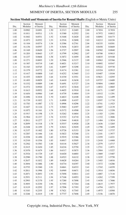
MOMENT OF INERTIA, SECTION MODULUS 255
Section Moduli and Moments of Inertia for Round Shafts (English or Metric Units)
Dia.Section
ModulusMomentof Inertia Dia.
SectionModulus
Momentof Inertia Dia.
SectionModulus
Momentof Inertia
1.00 0.0982 0.0491 1.50 0.3313 0.2485 2.00 0.7854 0.7854
1.01 0.1011 0.0511 1.51 0.3380 0.2552 2.01 0.7972 0.8012
1.02 0.1042 0.0531 1.52 0.3448 0.2620 2.02 0.8092 0.8173
1.03 0.1073 0.0552 1.53 0.3516 0.2690 2.03 0.8213 0.8336
1.04 0.1104 0.0574 1.54 0.3586 0.2761 2.04 0.8335 0.8501
1.05 0.1136 0.0597 1.55 0.3656 0.2833 2.05 0.8458 0.8669
1.06 0.1169 0.0620 1.56 0.3727 0.2907 2.06 0.8582 0.8840
1.07 0.1203 0.0643 1.57 0.3799 0.2982 2.07 0.8708 0.9013
1.08 0.1237 0.0668 1.58 0.3872 0.3059 2.08 0.8835 0.9188
1.09 0.1271 0.0693 1.59 0.3946 0.3137 2.09 0.8963 0.9366
1.10 0.1307 0.0719 1.60 0.4021 0.3217 2.10 0.9092 0.9547
1.11 0.1343 0.0745 1.61 0.4097 0.3298 2.11 0.9222 0.9730
1.12 0.1379 0.0772 1.62 0.4174 0.3381 2.12 0.9354 0.9915
1.13 0.1417 0.0800 1.63 0.4252 0.3465 2.13 0.9487 1.0104
1.14 0.1455 0.0829 1.64 0.4330 0.3551 2.14 0.9621 1.0295
1.15 0.1493 0.0859 1.65 0.4410 0.3638 2.15 0.9757 1.0489
1.16 0.1532 0.0889 1.66 0.4491 0.3727 2.16 0.9894 1.0685
1.17 0.1572 0.0920 1.67 0.4572 0.3818 2.17 1.0032 1.0885
1.18 0.1613 0.0952 1.68 0.4655 0.3910 2.18 1.0171 1.1087
1.19 0.1654 0.0984 1.69 0.4739 0.4004 2.19 1.0312 1.1291
1.20 0.1696 0.1018 1.70 0.4823 0.4100 2.20 1.0454 1.1499
1.21 0.1739 0.1052 1.71 0.4909 0.4197 2.21 1.0597 1.1710
1.22 0.1783 0.1087 1.72 0.4996 0.4296 2.22 1.0741 1.1923
1.23 0.1827 0.1124 1.73 0.5083 0.4397 2.23 1.0887 1.2139
1.24 0.1872 0.1161 1.74 0.5172 0.4500 2.24 1.1034 1.2358
1.25 0.1917 0.1198 1.75 0.5262 0.4604 2.25 1.1183 1.2581
1.26 0.1964 0.1237 1.76 0.5352 0.4710 2.26 1.1332 1.2806
1.27 0.2011 0.1277 1.77 0.5444 0.4818 2.27 1.1484 1.3034
1.28 0.2059 0.1318 1.78 0.5537 0.4928 2.28 1.1636 1.3265
1.29 0.2108 0.1359 1.79 0.5631 0.5039 2.29 1.1790 1.3499
1.30 0.2157 0.1402 1.80 0.5726 0.5153 2.30 1.1945 1.3737
1.31 0.2207 0.1446 1.81 0.5822 0.5268 2.31 1.2101 1.3977
1.32 0.2258 0.1490 1.82 0.5919 0.5386 2.32 1.2259 1.4221
1.33 0.2310 0.1536 1.83 0.6017 0.5505 2.33 1.2418 1.4468
1.34 0.2362 0.1583 1.84 0.6116 0.5627 2.34 1.2579 1.4717
1.35 0.2415 0.1630 1.85 0.6216 0.5750 2.35 1.2741 1.4971
1.36 0.2470 0.1679 1.86 0.6317 0.5875 2.36 1.2904 1.5227
1.37 0.2524 0.1729 1.87 0.6420 0.6003 2.37 1.3069 1.5487
1.38 0.2580 0.1780 1.88 0.6523 0.6132 2.38 1.3235 1.5750
1.39 0.2637 0.1832 1.89 0.6628 0.6264 2.39 1.3403 1.6016
1.40 0.2694 0.1886 1.90 0.6734 0.6397 2.40 1.3572 1.6286
1.41 0.2752 0.1940 1.91 0.6841 0.6533 2.41 1.3742 1.6559
1.42 0.2811 0.1996 1.92 0.6949 0.6671 2.42 1.3914 1.6836
1.43 0.2871 0.2053 1.93 0.7058 0.6811 2.43 1.4087 1.7116
1.44 0.2931 0.2111 1.94 0.7168 0.6953 2.44 1.4262 1.7399
1.45 0.2993 0.2170 1.95 0.7280 0.7098 2.45 1.4438 1.7686
1.46 0.3055 0.2230 1.96 0.7392 0.7244 2.46 1.4615 1.7977
1.47 0.3119 0.2292 1.97 0.7506 0.7393 2.47 1.4794 1.8271
1.48 0.3183 0.2355 1.98 0.7621 0.7545 2.48 1.4975 1.8568
1.49 0.3248 0.2419 1.99 0.7737 0.7698 2.49 1.5156 1.8870
Machinery's Handbook 27th Edition
Copyright 2004, Industrial Press, Inc., New York, NY
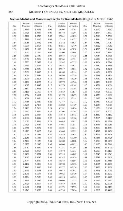
256 MOMENT OF INERTIA, SECTION MODULUS
Section Moduli and Moments of Inertia for Round Shafts (English or Metric Units)
Dia.Section
ModulusMomentof Inertia Dia.
SectionModulus
Momentof Inertia Dia.
SectionModulus
Momentof Inertia
2.50 1.5340 1.9175 3.00 2.6507 3.9761 3.50 4.2092 7.3662
2.51 1.5525 1.9483 3.01 2.6773 4.0294 3.51 4.2454 7.4507
2.52 1.5711 1.9796 3.02 2.7041 4.0832 3.52 4.2818 7.5360
2.53 1.5899 2.0112 3.03 2.7310 4.1375 3.53 4.3184 7.6220
2.54 1.6088 2.0432 3.04 2.7582 4.1924 3.54 4.3552 7.7087
2.55 1.6279 2.0755 3.05 2.7855 4.2479 3.55 4.3922 7.7962
2.56 1.6471 2.1083 3.06 2.8130 4.3038 3.56 4.4295 7.8844
2.57 1.6665 2.1414 3.07 2.8406 4.3604 3.57 4.4669 7.9734
2.58 1.6860 2.1749 3.08 2.8685 4.4175 3.58 4.5054 8.0631
2.59 1.7057 2.2089 3.09 2.8965 4.4751 3.59 4.5424 8.1536
2.60 1.7255 2.2432 3.10 2.9247 4.5333 3.60 4.5804 8.2248
2.61 1.7455 2.2779 3.11 2.9531 4.5921 3.61 4.6187 8.3368
2.62 1.7656 2.3130 3.12 2.9817 4.6514 3.62 4.6572 8.4295
2.63 1.7859 2.3485 3.13 3.0105 4.7114 3.63 4.6959 8.5231
2.64 1.8064 2.3844 3.14 3.0394 4.7719 3.64 4.7348 8.6174
2.65 1.8270 2.4208 3.15 3.0685 4.8329 3.65 4.7740 8.7125
2.66 1.8478 2.4575 3.16 3.0979 4.8946 3.66 4.8133 8.8083
2.67 1.8687 2.4947 3.17 3.1274 4.9569 3.67 4.8529 8.9050
2.68 1.8897 2.5323 3.18 3.1570 5.0197 3.68 4.8926 9.0025
2.69 1.9110 2.5703 3.19 3.1869 5.0831 3.69 4.9326 9.1007
2.70 1.9324 2.6087 3.20 3.2170 5.1472 3.70 4.9728 9.1998
2.71 1.9539 2.6476 3.21 3.2472 5.2118 3.71 5.0133 9.2996
2.72 1.9756 2.6869 3.22 3.2777 5.2771 3.72 5.0539 9.4003
2.73 1.9975 2.7266 3.23 3.3083 5.3429 3.73 5.0948 9.5018
2.74 2.0195 2.7668 3.24 3.3391 5.4094 3.74 5.1359 9.6041
2.75 2.0417 2.8074 3.25 3.3702 5.4765 3.75 5.1772 9.7072
2.76 2.0641 2.8484 3.26 3.4014 5.5442 3.76 5.2187 9.8112
2.77 2.0866 2.8899 3.27 3.4328 5.6126 3.77 5.2605 9.9160
2.78 2.1093 2.9319 3.28 3.4643 5.6815 3.78 5.3024 10.0216
2.79 2.1321 2.9743 3.29 3.4961 5.7511 3.79 5.3446 10.1281
2.80 2.1551 3.0172 3.30 3.5281 5.8214 3.80 5.3870 10.2354
2.81 2.1783 3.0605 3.31 3.5603 5.8923 3.81 5.4297 10.3436
2.82 2.2016 3.1043 3.32 3.5926 5.9638 3.82 5.4726 10.4526
2.83 2.2251 3.1486 3.33 3.6252 6.0360 3.83 5.5156 10.5625
2.84 2.2488 3.1933 3.34 3.6580 6.1088 3.84 5.5590 10.6732
2.85 2.2727 3.2385 3.35 3.6909 6.1823 3.85 5.6025 10.7848
2.86 2.2967 3.2842 3.36 3.7241 6.2564 3.86 5.6463 10.8973
2.87 2.3208 3.3304 3.37 3.7574 6.3313 3.87 5.6903 11.0107
2.88 2.3452 3.3771 3.38 3.7910 6.4067 3.88 5.7345 11.1249
2.89 2.3697 3.4242 3.39 3.8247 6.4829 3.89 5.7789 11.2401
2.90 2.3944 3.4719 3.40 3.8587 6.5597 3.90 5.8236 11.3561
2.91 2.4192 3.5200 3.41 3.8928 6.6372 3.91 5.8685 11.4730
2.92 2.4443 3.5686 3.42 3.9272 6.7154 3.92 5.9137 11.5908
2.93 2.4695 3.6178 3.43 3.9617 6.7943 3.93 5.9591 11.7095
2.94 2.4948 3.6674 3.44 3.9965 6.8739 3.94 6.0047 11.8292
2.95 2.5204 3.7176 3.45 4.0314 6.9542 3.95 6.0505 11.9497
2.96 2.5461 3.7682 3.46 4.0666 7.0352 3.96 6.0966 12.0712
2.97 2.5720 3.8194 3.47 4.1019 7.1168 3.97 6.1429 12.1936
2.98 2.5981 3.8711 3.48 4.1375 7.1992 3.98 6.1894 12.3169
2.99 2.6243 3.9233 3.49 4.1733 7.2824 3.99 6.2362 12.4412
Machinery's Handbook 27th Edition
Copyright 2004, Industrial Press, Inc., New York, NY
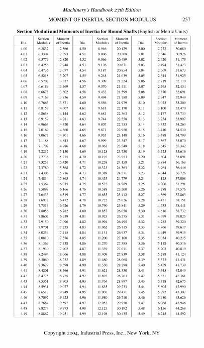
MOMENT OF INERTIA, SECTION MODULUS 257
Section Moduli and Moments of Inertia for Round Shafts (English or Metric Units)
Dia.Section
ModulusMomentof Inertia Dia.
SectionModulus
Momentof Inertia Dia.
SectionModulus
Momentof Inertia
4.00 6.2832 12.566 4.50 8.946 20.129 5.00 12.272 30.680
4.01 6.3304 12.693 4.51 9.006 20.308 5.01 12.346 30.926
4.02 6.3779 12.820 4.52 9.066 20.489 5.02 12.420 31.173
4.03 6.4256 12.948 4.53 9.126 20.671 5.03 12.494 31.423
4.04 6.4736 13.077 4.54 9.187 20.854 5.04 12.569 31.673
4.05 6.5218 13.207 4.55 9.248 21.039 5.05 12.644 31.925
4.06 6.5702 13.337 4.56 9.309 21.224 5.06 12.719 32.179
4.07 6.6189 13.469 4.57 9.370 21.411 5.07 12.795 32.434
4.08 6.6678 13.602 4.58 9.432 21.599 5.08 12.870 32.691
4.09 6.7169 13.736 4.59 9.494 21.788 5.09 12.947 32.949
4.10 6.7663 13.871 4.60 9.556 21.979 5.10 13.023 33.209
4.11 6.8159 14.007 4.61 9.618 22.170 5.11 13.100 33.470
4.12 6.8658 14.144 4.62 9.681 22.363 5.12 13.177 33.733
4.13 6.9159 14.281 4.63 9.744 22.558 5.13 13.254 33.997
4.14 6.9663 14.420 4.64 9.807 22.753 5.14 13.332 34.263
4.15 7.0169 14.560 4.65 9.871 22.950 5.15 13.410 34.530
4.16 7.0677 14.701 4.66 9.935 23.148 5.16 13.488 34.799
4.17 7.1188 14.843 4.67 9.999 23.347 5.17 13.567 35.070
4.18 7.1702 14.986 4.68 10.063 23.548 5.18 13.645 35.342
4.19 7.2217 15.130 4.69 10.128 23.750 5.19 13.725 35.616
4.20 7.2736 15.275 4.70 10.193 23.953 5.20 13.804 35.891
4.21 7.3257 15.420 4.71 10.258 24.158 5.21 13.884 36.168
4.22 7.3780 15.568 4.72 10.323 24.363 5.22 13.964 36.446
4.23 7.4306 15.716 4.73 10.389 24.571 5.23 14.044 36.726
4.24 7.4834 15.865 4.74 10.455 24.779 5.24 14.125 37.008
4.25 7.5364 16.015 4.75 10.522 24.989 5.25 14.206 37.291
4.26 7.5898 16.166 4.76 10.588 25.200 5.26 14.288 37.576
4.27 7.6433 16.319 4.77 10.655 25.412 5.27 14.369 37.863
4.28 7.6972 16.472 4.78 10.722 25.626 5.28 14.451 38.151
4.29 7.7513 16.626 4.79 10.790 25.841 5.29 14.533 38.441
4.30 7.8056 16.782 4.80 10.857 26.058 5.30 14.616 38.732
4.31 7.8602 16.939 4.81 10.925 26.275 5.31 14.699 39.025
4.32 7.9150 17.096 4.82 10.994 26.495 5.32 14.782 39.320
4.33 7.9701 17.255 4.83 11.062 26.715 5.33 14.866 39.617
4.34 8.0254 17.415 4.84 11.131 26.937 5.34 14.949 39.915
4.35 8.0810 17.576 4.85 11.200 27.160 5.35 15.034 40.215
4.36 8.1369 17.738 4.86 11.270 27.385 5.36 15.118 40.516
4.37 8.1930 17.902 4.87 11.339 27.611 5.37 15.203 40.819
4.38 8.2494 18.066 4.88 11.409 27.839 5.38 15.288 41.124
4.39 8.3060 18.232 4.89 11.480 28.068 5.39 15.373 41.431
4.40 8.3629 18.398 4.90 11.550 28.298 5.40 15.459 41.739
4.41 8.4201 18.566 4.91 11.621 28.530 5.41 15.545 42.049
4.42 8.4775 18.735 4.92 11.692 28.763 5.42 15.631 42.361
4.43 8.5351 18.905 4.93 11.764 28.997 5.43 15.718 42.675
4.44 8.5931 19.077 4.94 11.835 29.233 5.44 15.805 42.990
4.45 8.6513 19.249 4.95 11.907 29.471 5.45 15.892 43.307
4.46 8.7097 19.423 4.96 11.980 29.710 5.46 15.980 43.626
4.47 8.7684 19.597 4.97 12.052 29.950 5.47 16.068 43.946
4.48 8.8274 19.773 4.98 12.125 30.192 5.48 16.156 44.268
4.49 8.8867 19.951 4.99 12.198 30.435 5.49 16.245 44.592
Machinery's Handbook 27th Edition
Copyright 2004, Industrial Press, Inc., New York, NY

258 MOMENT OF INERTIA, SECTION MODULUS
Section Moduli and Moments of Inertia for Round Shafts (English or Metric Units)
Dia.Section
ModulusMomentof Inertia Dia.
SectionModulus
Momentof Inertia Dia.
SectionModulus
Momentof Inertia
5.5 16.3338 44.9180 30 2650.72 39760.8 54.5 15892.4 433068
6 21.2058 63.6173 30.5 2785.48 42478.5 55 16333.8 449180
6.5 26.9612 87.6241 31 2924.72 45333.2 55.5 16783.4 465738
7 33.6739 117.859 31.5 3068.54 48329.5 56 17241.1 482750
7.5 41.4175 155.316 32 3216.99 51471.9 56.5 17707.0 500223
8 50.2655 201.062 32.5 3370.16 54765.0 57 18181.3 518166
8.5 60.2916 256.239 33 3528.11 58213.8 57.5 18663.9 536588
9 71.5694 322.062 33.5 3690.92 61822.9 58 19155.1 555497
9.5 84.1726 399.820 34 3858.66 65597.2 58.5 19654.7 574901
10 98.1748 490.874 34.5 4031.41 69541.9 59 20163.0 594810
10.5 113.650 596.660 35 4209.24 73661.8 59.5 20680.0 615230
11 130.671 718.688 35.5 4392.23 77962.1 60 21205.8 636173
11.5 149.312 858.541 36 4580.44 82448.0 60.5 21740.3 657645
12 169.646 1017.88 36.5 4773.96 87124.7 61 22283.8 679656
12.5 191.748 1198.42 37 4972.85 91997.7 61.5 22836.3 702215
13 215.690 1401.98 37.5 5177.19 97072.2 62 23397.8 725332
13.5 241.547 1630.44 38 5387.05 102354 62.5 23968.4 749014
14 269.392 1885.74 38.5 5602.50 107848 63 24548.3 773272
14.5 299.298 2169.91 39 5823.63 113561 63.5 25137.4 798114
15 331.340 2485.05 39.5 6050.50 119497 64 25735.9 823550
15.5 365.591 2833.33 40 6283.19 125664 64.5 26343.8 849589
16 402.124 3216.99 40.5 6521.76 132066 65 26961.2 876241
16.5 441.013 3638.36 41 6766.30 138709 65.5 27588.2 903514
17 482.333 4099.83 41.5 7016.88 145600 66 28224.9 931420
17.5 526.155 4603.86 42 7273.57 152745 66.5 28871.2 959967
18 572.555 5153.00 42.5 7536.45 160150 67 29527.3 989166
18.5 621.606 5749.85 43 7805.58 167820 67.5 30193.3 1019025
19 673.381 6397.12 43.5 8081.05 175763 68 30869.3 1049556
19.5 727.954 7097.55 44 8362.92 183984 68.5 31555.2 1080767
20 785.398 7853.98 44.5 8651.27 192491 69 32251.3 1112670
20.5 845.788 8669.33 45 8946.18 201289 69.5 32957.5 1145273
21 909.197 9546.56 45.5 9247.71 210385 70 33673.9 1178588
21.5 975.698 10488.8 46 9555.94 219787 70.5 34400.7 1212625
22 1045.36 11499.0 46.5 9870.95 229499 71 35137.8 1247393
22.5 1118.27 12580.6 47 10192.8 239531 71.5 35885.4 1282904
23 1194.49 13736.7 47.5 10521.6 249887 72 36643.5 1319167
23.5 1274.10 14970.7 48 10857.3 260576 72.5 37412.3 1356194
24 1357.17 16286.0 48.5 11200.2 271604 73 38191.7 1393995
24.5 1443.77 17686.2 49 11550.2 282979 73.5 38981.8 1432581
25 1533.98 19174.8 49.5 11907.4 294707 74 39782.8 1471963
25.5 1627.87 20755.4 50 12271.8 306796 74.5 40594.6 1512150
26 1725.52 22431.8 50.5 12643.7 319253 75 41417.5 1553156
26.5 1827.00 24207.7 51 13023.0 332086 75.5 42251.4 1594989
27 1932.37 26087.0 51.5 13409.8 345302 76 43096.4 1637662
27.5 2041.73 28073.8 52 13804.2 358908 76.5 43952.6 1681186
28 2155.13 30171.9 52.5 14206.2 372913 77 44820.0 1725571
28.5 2272.66 32385.4 53 14616.0 387323 77.5 45698.8 1770829
29 2394.38 34718.6 53.5 15033.5 402147 78 46589.0 1816972
29.5 2520.38 37175.6 54 15459.0 417393 78.5 47490.7 1864011
Machinery's Handbook 27th Edition
Copyright 2004, Industrial Press, Inc., New York, NY
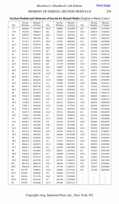
MOMENT OF INERTIA, SECTION MODULUS 259
Section Moduli and Moments of Inertia for Round Shafts (English or Metric Units)
Dia.Section
ModulusMomentof Inertia Dia.
SectionModulus
Momentof Inertia Dia.
SectionModulus
Momentof Inertia
79 48404.0 1911958 103.5 108848 5632890 128 205887 13176795
79.5 49328.9 1960823 104 110433 5742530 128.5 208310 13383892
80 50265.5 2010619 104.5 112034 5853762 129 210751 13593420
80.5 51213.9 2061358 105 113650 5966602 129.5 213211 13805399
81 52174.1 2113051 105.5 115281 6081066 130 215690 14019848
81.5 53146.3 2165710 106 116928 6197169 130.5 218188 14236786
82 54130.4 2219347 106.5 118590 6314927 131 220706 14456231
82.5 55126.7 2273975 107 120268 6434355 131.5 223243 14678204
83 56135.1 2329605 107.5 121962 6555469 132 225799 14902723
83.5 57155.7 2386249 108 123672 6678285 132.5 228374 15129808
84 58188.6 2443920 108.5 125398 6802818 133 230970 15359478
84.5 59233.9 2502631 109 127139 6929085 133.5 233584 15591754
85 60291.6 2562392 109.5 128897 7057102 134 236219 15826653
85.5 61361.8 2623218 110 130671 7186884 134.5 238873 16064198
86 62444.7 2685120 110.5 132461 7318448 135 241547 16304406
86.5 63540.1 2748111 111 134267 7451811 135.5 244241 16547298
87 64648.4 2812205 111.5 136089 7586987 136 246954 16792893
87.5 65769.4 2877412 112 137928 7723995 136.5 249688 17041213
88 66903.4 2943748 112.5 139784 7862850 137 252442 17292276
88.5 68050.2 3011223 113 141656 8003569 137.5 255216 17546104
89 69210.2 3079853 113.5 143545 8146168 138 258010 17802715
89.5 70383.2 3149648 114 145450 8290664 138.5 260825 18062131
90 71569.4 3220623 114.5 147372 8437074 139 263660 18324372
90.5 72768.9 3292791 115 149312 8585414 139.5 266516 18589458
91 73981.7 3366166 115.5 151268 8735703 140 269392 18857410
91.5 75207.9 3440759 116 153241 8887955 140.5 272288 19128248
92 76447.5 3516586 116.5 155231 9042189 141 275206 19401993
92.5 77700.7 3593659 117 157238 9198422 141.5 278144 19678666
93 78967.6 3671992 117.5 159262 9356671 142 281103 19958288
93.5 80248.1 3751598 118 161304 9516953 142.5 284083 20240878
94 81542.4 3832492 118.5 163363 9679286 143 287083 20526460
94.5 82850.5 3914688 119 165440 9843686 143.5 290105 20815052
95 84172.6 3998198 119.5 167534 10010172 144 293148 21106677
95.5 85508.6 4083038 120 169646 10178760 144.5 296213 21401356
96 86858.8 4169220 120.5 171775 10349469 145 299298 21699109
96.5 88223.0 4256760 121 173923 10522317 145.5 302405 21999959
97 89601.5 4345671 121.5 176088 10697321 146 305533 22303926
97.5 90994.2 4435968 122 178270 10874498 146.5 308683 22611033
98 92401.3 4527664 122.5 180471 11053867 147 311854 22921300
98.5 93822.8 4620775 123 182690 11235447 147.5 315047 23234749
99 95258.9 4715315 123.5 184927 11419254 148 318262 23551402
99.5 96709.5 4811298 124 187182 11605307 148.5 321499 23871280
100 98174.8 4908739 124.5 189456 11793625 149 324757 24194406
100.5 99654.8 5007652 125 191748 11984225 149.5 328037 24520802
101 101150 5108053 125.5 194058 12177126 150 331340 24850489
101.5 102659 5209956 126 196386 12372347 … … …
102 104184 5313376 126.5 198734 12569905 … … …
102.5 105723 5418329 127 201100 12769820 … … …
103 107278 5524828 127.5 203484 12972110 … … …
Machinery's Handbook 27th Edition
Copyright 2004, Industrial Press, Inc., New York, NY
Next page