Mechanics of Materials 42 (2010) 709–725

Contents lists available at ScienceDirect

Mechanics of Materials

journal homepage: www.elsevier .com/locate /mechmat

Analysis of the elastostatic specific stiffness of 2D stretching-dominatedlattice materials

Mostafa S.A. Elsayed, Damiano Pasini *

Department of Mechanical Engineering, McGill University, Montreal, Que., Canada H3A 2K6

a r t i c l e i n f o

Article history:Received 3 September 2009Received in revised form 6 May 2010

Keywords:Lattice materialMicro-trussBloch’s theoremDummy Node SchemeStretching-dominated lattice material

0167-6636/$ - see front matter Crown Copyright �doi:10.1016/j.mechmat.2010.05.003

* Corresponding author.E-mail address: damiano.pasini@mcgill.ca (D. Pa

a b s t r a c t

This paper presents a matrix-based procedure to characterize the specific stiffness proper-ties of 2D lattice materials with any arbitrary cell topology. Unlike previous works, the cur-rent study automates the analysis process to include lattice materials whose unit cell haselements extending between adjacent cells and thus intersecting their envelopes. The mainchallenge in the analysis of this periodic lattice structures is that the unit cell does not havethe full information concerning its nodal kinematic and static periodicity. For this reason,we introduce the Dummy Node Scheme, which enables the analysis of lattice material withany cell topology.

The lattice material is modelled here as a pin-jointed infinite micro-truss structure. Theresults of the determinacy analysis are used to distinguish between the bending-domi-nated and the stretching-dominated behaviours of the material. The Cauchy–Born hypoth-esis is used to homogenize the lattice material properties by formulating the microscopiclattice nodal deformations in terms of the material macroscopic strain field. This formula-tion, in turn, is used to express the microscopic element deformations in terms of the mac-roscopic strain field, from which the material macroscopic stiffness properties are derived.In this process, the Dummy Node Scheme is a necessary step to construct the nodal period-icity within the unit cell, which is used to apply the Cauchy–Born kinematic boundary con-dition to the nodal deformation wave functions. The procedure introduced in this paper isapplied to 10 lattice topologies, five of which have unit cells with a square Bravais latticesymmetry and the other five have unit cells with a hexagonal Bravais lattice symmetry.Finally, charts representing the relative elastic moduli of the lattice material versus its rel-ative density are developed. These charts assist the selection of the best topology of astretching-dominated lattice material for a given application that requires a material withspecific stiffness properties.

Crown Copyright � 2010 Published by Elsevier Ltd. All rights reserved.

1. Introduction metries in 2D. In this study, we consider only lattice unit

A lattice material is a type of cellular material withperiodic microstructure. The unit cell is the building blockused to tessellate the space into a periodic modular pat-tern. An important condition to generate a consistent tes-sellation is that the unit cell should have a minimumlevel of symmetry, as defined by the Bravais lattice sym-metry (Brillouin, 1946). There are five Bravais lattice sym-

2010 Published by Elsevier

sini).

cells with hexagonal and square Bravais lattice symme-tries. Several 2D lattice materials with hexagonal as wellsquare Bravais lattice symmetry have been introducedin the literatures (Hutchinson and Fleck, 2006; Phaniet al., 2006; Hutchinson, 2004; Alethea, 2004). The formerincludes the regular fully triangulated lattice, the regularhexagonal lattice and the semi-regular Kagome’ lattice,which have the modified Schläfli symbols of 36, 63 and3.6.3.6, respectively. The latter consists of the regularsquare lattice, the rectangular lattice and the doublebraced square lattice.

Ltd. All rights reserved.

710 M.S.A. Elsayed, D. Pasini / Mechanics of Materials 42 (2010) 709–725

A lattice material can be classified into bending andstretching-dominated materials with respect to the micro-scopic failure mode of the unit cell elements. Microscopicstructural analysis shows that the bending-dominated lat-tice material has a low nodal connectivity at the cell verti-ces, which results in a microscopic bending-dominatedfailure mode, where the cell elements collapse by bendingstresses. This feature generates non-optimal mechanicalproperties where the element solid materials are not fullyemployed in the microscopic loading resistance. On thecontrary, the stretching-dominated lattice material has ahigh nodal connectivity at the cell vertices, which resultsin microscopic stretching-dominated failure mode wherethe cell elements collapse by axial stresses, giving a muchhigher stiffness and strength per unit mass. For instance,the structural analysis of stretching-dominated latticematerial shows that its stiffness and strength scale up withthe density ratio of the lattice material to the solid mate-rial, �q; on the other hand, the stiffness and the strengthof the bending-dominated material are governed, respec-tively, by �q2 and �q3=2 (Gibson and Ashby, 1997). The differ-ent scaling laws have a strong impact on the strength andstiffness of the material. For example, at �q ¼ 0:01, thestretching-dominated lattice material has superior staticperformance because it is 100 times stiffer and 10 timesstronger than the bending-dominated material.

To distinguish between bending and stretching-domi-nated lattice materials, we resort to the analysis of thekinematic determinacy of the pin-jointed version of thelattice micro structure. Maxwell (1864) set a rule for theminimum number of bars necessary for a pin-jointedframework to be kinematically determinate; these mini-mum numbers of bars are, (2j � 3) and (3j � 6) in 2D and3D frameworks, respectively, where j is the number ofjoints within a finite framework. A framework with lessnumber of bars than the minimum condition of Maxwellis a mechanism, unless its joints are set to be rigid; in thiscase the framework behaviour is bending-dominated. Call-adine (1978) and Pellegrino and Calladine (1986) and Pel-legrino (1993) reviewed the linear-algebraic basis ofMaxwell’s rule using the fundamental subspaces of theequilibrium and the kinematic matrices of a pin-jointedframework. As a result, they reformulated the problem toobtain the generalization of Maxwell’s rule, which includesinformation about the states of self-stress and the states ofinternal mechanisms within the framework. A state of self-stress is the vector of element forces generated within anunloaded framework; on the other hand, a state of internalmechanism is the vector of joint displacements corre-sponding to non-deforming elements. The generalizedMaxwell’s rule can be used to obtain an accurate predic-tion of the determinacy state of finite lattice structures inthe form of a unit cell or a finite cluster of cells. Since thelattice material is structured at the microscale while itseffective properties are homogenized at the macroscale,the analysis of the lattice material assumes a periodicityof the unit cell in an unbounded space. Therefore a com-plete determinacy analysis of lattice materials requiresextending the analysis to the infinite lattice structure. Suchan extension was proposed by Deshpande et al. (2001) whoexamined the pin-jointed mechanics of a restricted set of

infinite-periodic lattice topologies. They considered onlytopologies wherein the joints are similarly situated, i.e.the framework appears the same and in the same orienta-tion regardless of the viewpoint. In 2D, these are the regu-lar square and triangular lattices; in 3D, this set includesthe regular octet-truss. The generalized Maxwell’s rule,was used to prove that the necessary but not sufficient no-dal connectivity, Z, of a structure to be stretching-domi-nated is Z = 4 and Z = 6 in 2D and 3D, respectively. On theother hand, the sufficient nodal connectivity was provento be Z = 6 and Z = 12 in 2D and 3D, respectively. More re-cently, Hutchinson (2004) used the Bloch’s theorem formodelling periodic waves in an infinite lattice structurewith any Bravais symmetry. His analysis focused mainlyon the case where the cell elements of the lattice sharetheir end points with those of the cell envelope. However,a procedure to analyze lattice materials whose unit cellelements intersect their envelopes need to be formulated.

In this work, the analysis of lattice materials is extendedto consider the case where some of the cell elements donot intersect the cell envelope at their end joints. For thispurpose, we introduce the Dummy Node Scheme, whichconsists of adding dummy nodes at the points of intersec-tion between the microscopic cell elements and the cellenvelope. These dummy nodes are used to generate thekinematic and the equilibrium matrices of the unit cell fi-nite microstructure. In addition, they are also used to gen-erate an explicit expression for the microscopic nodaldeformations in terms of a macroscopic hypotheticalhomogeneous strain field, as assumed by the Cauchy–Bornhypothesis (Bhattacharya, 2003). The degrees of freedomassociated with the hypothetical dummy nodes are laterremoved from the generated matrix systems. This proce-dure is integrated in a matrix formulation for a compre-hensive structural analysis of different lattice topologies.The results are then plotted in design charts that help togain insight into the stiffness generated by the consideredcell topologies.

Organized in four sections, the paper introduces thetheoretical analysis and the description of the systematicprocedure in Section 2. In Section 3, this procedure is ap-plied to the different topologies with hexagonal and squareBravais lattice symmetries. Section 3.2 compares the char-acterized stiffness properties before presenting the con-cluding remarks in Section 4.

2. Analysis

Notions of solid-state physics can help in solid mechan-ics to examine the characteristics of lattice materials. Prin-ciples of symmetry, for example, are often used in solid-state physics to simplify the formulation of the governinglaw of crystals. In this paper, we adopt the classical notionof a crystal structure, which can be described by introduc-ing two characterizing parameters as (Brillouin, 1946):

Crystal ¼ Latticeþ Bases ð1Þ

The lattice is defined as a translational infinitely periodicarrangement of points (Grosso and Pastori-Parravincini,2000; Jones and March, 1973). When periods of the unit

2→a

(b)

1→a

Cell envelope

Square crystal

(A)

(B)

(a)

Crystal Bases

mb

ljy

x (0,0)

(B)

(d)

mb

ljy

x (0,0) (A)

(c)

Fig. 1. 2D Square lattice structure.

M.S.A. Elsayed, D. Pasini / Mechanics of Materials 42 (2010) 709–725 711

cell are perfectly stacked in two or three dimension, thespace is told to be tessellated. The bases are the mathemat-ical representation for the physical constituents that arerepeated in every cell translation.

In continuum mechanics, a lattice material can be char-acterized by adopting the above definition. The cell envel-op, which defines the structure periodicity, is described inmathematical terms by the lattice translational symmetryprimitive bases, a

!k, where k 2 {1, . . .,n} and n = 2 or n = 3

in 2D or 3D, respectively. The set of bases, representingthe physical structure, contains two groups, namely, thejoint bases group and the bar bases group.

Fig. 1 illustrates this concept, as applied to the squarelattice. Fig. 1a shows the microscopic crystal structure ofthe lattice material, where two candidate unit cells (A)and (B) are shown (within the dotted envelope). Fig. 1bshows the lattice translational symmetry primitive basesa!

1 and a!

2. Fig. 1c and d illustrates the physical structurebar position vectors, b

!m, and joint position vectors, j

!l, of

the candidate unit cells, (A) and (B), respectively, wherem 2 {1,2, . . .,b} and l 2 {1,2, . . ., j}. b and j are the total num-ber of bars and joints within the unit cell structure,respectively.

2.1. Unit cell determinacy analysis

Following the approach by Calladine (1978), Pellegrinoand Calladine (1986) and Pellegrino (1993), we considera finite truss structure that consists of j total joints con-nected by b bars. The b bar tension forces and displacementdeformations are assembled into vectors t and e, respec-tively. On the other hand, the nj components of externalforce and joint displacements are assembled into vectorsf and d, respectively. The equilibrium and the kinematicsystems of the truss structure are expressed as:

A � t ¼ f ð2aÞB � d ¼ e ð2bÞ

where A 2 R(nj)�b is the equilibrium matrix and B 2 Rb�(nj)isthe kinematic matrix. The formulation of the equilibriumand the kinematic matrices for the unit cell shown inFig. 1c is straightforward. However, to generate the equi-librium and the kinematic matrices of the unit cell illus-trated in Fig. 1d, we need to introduce an alternativeprocedure, as explained in the following.

ib

ijy

x (0,0) idj

Fig. 2. Dummy nodes (j) added to the unit cell.

2.1.1. Dummy Node SchemeThe Dummy Node Scheme is introduced to deal with lat-

tice structures containing structural elements extendingbetween adjacent unit cells. The derivation and theoreticalanalysis of this scheme is detailed in Appendix A. Here, wedescribe the steps required to apply the Dummy NodeScheme.

Step 1: Hypothetical dummy nodes are introduced atthe intersection points between the microscopic cell ele-ments, extending between neighbouring unit cells, andthe cell envelope. The kinematic and the equilibriummatrices of the finite microstructure are then reformulatedto take into account the dummy nodes.

Step 2: Once the kinematic and the equilibrium systemsare formulated, the degrees of freedom associated with thedummy nodes are eliminated from the generated matrices.The degrees of freedom associated with the dummy nodesare expressed in the row space of the equilibrium matrix,given in Eq. (2a), as well as in the column space of the kine-matic matrix, given in Eq. (2b). To eliminate the degrees offreedom associated with the dummy nodes, all modes inthe row space of the equilibrium matrix and the columnspace of the kinematic matrix that are associated withthe dummy nodes are eliminated. The same eliminationtechnique is applied to the nodal force and the nodal dis-placement vectors.

As an example, consider the unit cell, (B), shown inFig. 1d. The above steps are applied as follows:

Step 1: Four dummy nodes are defined for the unit cell(B) as shown in Fig. 2. It should be noted that in this casethe dummy node position vectors are coincident with theposition vectors of the bars that intersect with the cellenvelope and the total group of joint position vectorsnow includes also the dummy nodes position vectors.Using this new group of joint position vectors along withthe group of bar position vectors, the equilibrium and thekinematic matrices of the unit cell structure can be formu-lated as:

712 M.S.A. Elsayed, D. Pasini / Mechanics of Materials 42 (2010) 709–725

�1 0 1 00 �1 0 10 0 �1 00 0 0 00 0 0 00 0 0 �11 0 0 00 0 0 00 0 0 00 1 0 0

26666666666666666664

37777777777777777775

t1

t2

t3

t4

2666666

3777777 ¼

f1x

f1y

fd1x

fd1y

fd2x

fd2y

fd3x

fd3y

fd4x

fd4y

2666666666666666666666

3777777777777777777777

ð3aÞ

�1 0 1 00 �1 0 10 0 �1 00 0 0 00 0 0 00 0 0 �11 0 0 00 0 0 00 0 0 00 1 0 0

26666666666666666664

37777777777777777775

T d1x

d1y

dd1x

dd1y

dd2x

dd2y

dd3x

dd3y

dd4x

dd4y

2666666666666666666666

3777777777777777777777

¼

e1

e2

e3

e4

2666666

3777777ð3bÞ

where fd and dd are dummy node forces and deformations,respectively.

Step 2: the degrees of freedom associated with the dum-my nodes are now eliminated from the matrix systems ofEq. (3), which results in:

�1 0 1 00 �1 0 1

� � t1

t2

t3

t4

2666666

3777777 ¼f1x

f1y

� �ð4aÞ

�1 00 �11 00 1

2666437775 d1x

d1y

� �¼

e1

e2

e3

e4

2666666

3777777 ð4bÞ

Eq. (4) shows, respectively, the equilibrium and the kine-matic systems of the unit cell shown in Fig. 1d.

For the determinacy analysis of the structure, we resortto the classical four fundamental vector subspaces of thekinematic and the equilibrium matrices (Pellegrino andCalladine, 1986).

It should be noted that, for the determinacy analysis ofthe unit cell finite structure, the computation of the fourfundamental subspaces must be applied to the equilibriumand the kinematic matrices that include the degrees offreedom associated with the dummy nodes, e.g. the matri-ces given in Eq. (3) for the square lattice. The reason forthis is that the elimination of the dummy nodes from thematrix system of the finite structure acts as the applicationof boundary conditions that fix the finite structure into afoundation which results in inaccurate results. However,for the determinacy analysis of the infinite lattice struc-ture, the reduced forms of the kinematic and the equilib-

rium matrices, e.g. the matrices given in Eq. (4) for thesquare lattice, are used.

2.2. Infinite structure determinacy analysis

Hutchinson (2004) first applied the Bloch’s theorem tothe determinacy analysis of the infinite lattice structure.The Bloch’s theorem requires the definition of a set ofparameters to describe a wave- function over the infinitelattice structure. The same approach is used in this workand the relevant lattice parameters are briefly definedhere.

2.2.1. Direct translational basesThe lattice translational symmetry primitive bases, a

!k,

are referred to as the direct translational bases, which gov-ern the process of the cell tessellation.

2.2.2. Direct translational vectorA direct translational vector is formulated as a linear

combination of direct translational bases; this vector isused to translate the reference unit cell to any other cellin the space of the lattice. The direct translational vectoris formulated as:

R!¼Xn

k¼1

mk a!

k ð5Þ

where mk is any set of integers and n is the dimensionalspace of the lattice. It should be noted that the direct trans-lational vector is the Bravais lattice vector spanned over aset of cells in the lattice space.

2.2.3. Position vectorsBy using the definition of bar and joint bases of the ref-

erence unit cell envelope, along with the definition of thedirect translational vector, the position vectors of barsand joints of the whole crystal structure can be formulatedas:

pl ¼ jl þ R!¼ jl þ

Xn

k¼1

mk a!

k 8l 2 1; . . . ; Jf g;

k 2 f1; . . . ;ng; n ¼ 2 in 2D and n ¼ 3 in 3D and mk 2 Z

ð6aÞ

qm ¼ bm þ R!¼ bm þ

Xn

k¼1

mk a!

k 8m 2 f1; . . . ;Bg;

k 2 f1; . . . ;ng; n ¼ 2 in 2D and n ¼ 3 in 3D and mk 2 Z

ð6bÞ

where pl and qm are the joints and the bars position vec-tors, respectively. J and B are, respectively, the number ofindependent joints and the number of independent bars,within the reference unit cell envelope.

2.2.4. Direct latticeThe direct lattice contains the set of independent bar

and joint bases, over the reference unit cell envelope,spanned over the infinite-periodic lattice structure by theirposition vectors. This set of infinite bases is called the

qL

qLT qT qRT

qLB qB qRB

qI qR

x

y

Fig. 3. Generic unit cell with its periodic displacement boundaryconditions.

M.S.A. Elsayed, D. Pasini / Mechanics of Materials 42 (2010) 709–725 713

direct lattice. To determine the independent set of bar andjoint bases over the reference unit cell, we verify thedependency of the bases within the reference unit cellthrough the relation:

Vi�1 ¼ Vi þXn

k¼1

xk a!

k ð7Þ

where xk 2 f�1;0;1g is a unit translation vector, If Vi�1 andVi belong to the joint position vectors, then Vi � jl andi � l 2 {1, . . ., J} and if they belong to the bar position vec-tors, then Vi � bm and i �m 2 {1, . . .,B}. The dependencyinformation is used later to modify the wave- function overthe reference unit cell to generate the periodic wave- func-tion over the infinite lattice.

2.2.5. Reciprocal latticeThe reciprocal lattice is itself a Bravais lattice intro-

duced to describe the lattice in terms of primitive vectors.The advantage of resorting to the reciprocal lattice is todiscretize the continuous space of the lattice into a discretesummation of modes at which the lattice performance canbe examined. The reciprocal lattice can be represented bythe primitive vectors b

!1 and b

!2, which are defined as:

b!

i � a!

j ¼ 2pdij ð8Þ

where a!

j and b!

i are the direct and the reciprocal latticebases, respectively, and i, j 2 {1,2} in 2D. dij is the Kroneckerdelta symbol that satisfies:

dij ¼0 for i– j

1 for i ¼ j

�ð9Þ

Thus, the translational vectors of the reciprocal lattice aredefined as:

x ¼ x1 b!

1 þx2 b!

2 8x1;x2 2 ½0;1Þ � Q ð10Þ

where x1 and x2 are the covariant components of x withrespect to the basis b

!1 and b

!2 and Q is the set of all rational

numbers. x1 and x2 are defined over the open subset of Qfrom zero to near unity in agreement with the Bloch’s the-orem (Hutchinson, 2004), described in the followingsection.

2.2.6. Bloch’s theoremThe Bloch’s theorem is used to extend the determinacy

analysis of the unit cell to the unbounded periodic lattice.

2.2.6.1. Bloch-wave mechanisms and states of self-stress. TheBloch’s theorem is applied to define the propagation of awave function over the infinite lattice structure. For nodaldeformation functions, the generalized nodal displacementvectors d(pl,x) 2 C2 can be expressed over the entire latticeas a wave function of the form:

dðpl;xÞ ¼ d jl þ R!;x

� �¼ dðjl;xÞe2pix R

!

8l 2 1;2; . . . ; Jf g

ð11aÞ

where J is the number of independent nodes within theunit cell envelope, pl ¼ jl þ R

!is the position vector of any

node throughout the lattice and R!

is the Bravais cell vectorof any unit cell through the entire lattice.

Similarly, for bar deformation functions, the generalizedbar deformation vectors e(qm,x) 2 C2 can be expressedover the entire lattice as a wave function of the form:

eðqm;xÞ ¼ e bmþ R!;x

� �¼ eðbm;xÞe2pix R

!

8m2 f1;2; . . . ;Bg

ð11bÞ

where B is the number of independent bars within the unitcell envelope and qm ¼ bm þ R

!is the position vector of any

bar throughout the lattice.To reduce the forms of the kinematic and the equilib-

rium matrices, we define transformation matrices for bothbars and joints. This procedure makes use of the periodicboundary conditions defined over the unit cell (Langley,1993; Langley et al., 1997).

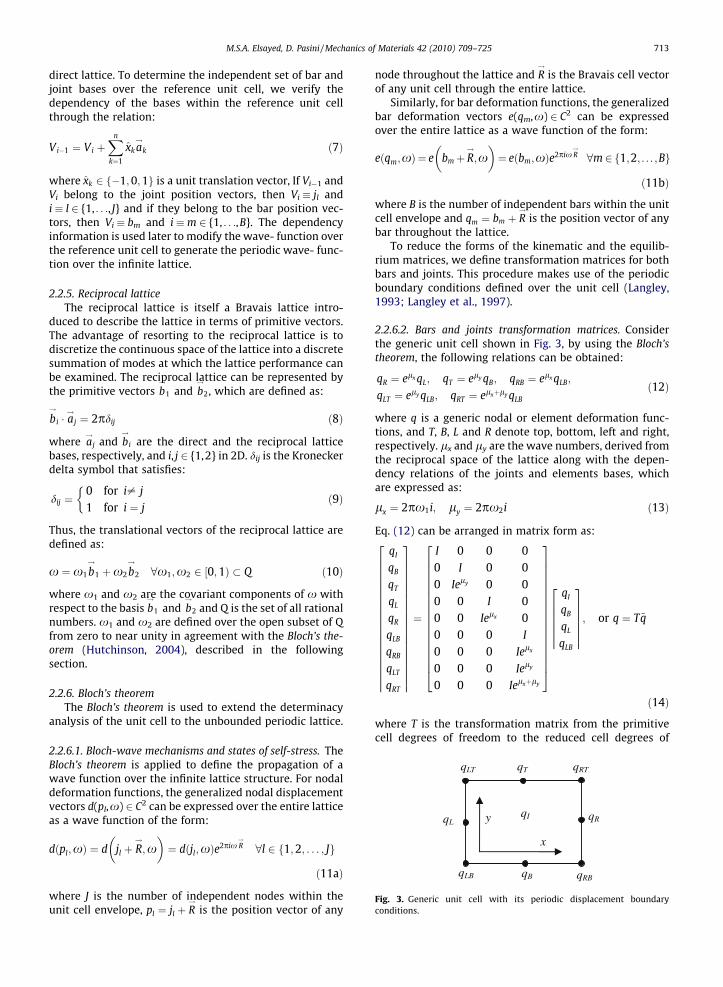
2.2.6.2. Bars and joints transformation matrices. Considerthe generic unit cell shown in Fig. 3, by using the Bloch’stheorem, the following relations can be obtained:

qR ¼ elx qL; qT ¼ ely qB; qRB ¼ elx qLB;

qLT ¼ ely qLB; qRT ¼ elxþly qLB

ð12Þ

where q is a generic nodal or element deformation func-tions, and T, B, L and R denote top, bottom, left and right,respectively. lx and ly are the wave numbers, derived fromthe reciprocal space of the lattice along with the depen-dency relations of the joints and elements bases, whichare expressed as:

lx ¼ 2px1i; ly ¼ 2px2i ð13Þ

Eq. (12) can be arranged in matrix form as:

qI

qB

qT

qL

qR

qLB

qRB

qLT

qRT

26666666666666666666

37777777777777777777

¼

I 0 0 00 I 0 00 Iely 0 00 0 I 00 0 Ielx 00 0 0 I

0 0 0 Ielx

0 0 0 Iely

0 0 0 Ielxþly

266666666666666664

377777777777777775

qI

qB

qL

qLB

2666666

3777777; or q ¼ T~q

ð14Þ

where T is the transformation matrix from the primitivecell degrees of freedom to the reduced cell degrees of

714 M.S.A. Elsayed, D. Pasini / Mechanics of Materials 42 (2010) 709–725

freedom. The transformation matrices for the elementdeformations and the nodal displacements wave functionsare obtained such that:

e ¼ Te~e ð15aÞd ¼ Td

~d ð15bÞ

where ~e and ~d are the element deformations and the nodaldisplacements reduced vectors (periodic wave function),respectively. Te and Td are the matrices that transforms,respectively, the full vectors of the periodic element defor-mations and nodal displacements to their respective re-duced periodic vectors.

The technique described above to generate the transfor-mation matrices is applied to the generic unit cell shown inFig. 3. The transformation matrices are generated takinginto account the dependency relations of the bars andthe joints bases. These dependency relations are computedby Eq. (7). The key parameter in Eq. (7) is the direct trans-lational bases, a

!k, which is formulated through the lattice

symmetry and the unit cell geometry. Details about thetechnique used to formulate the transformation matricesare given in Appendix B.

Substituting Eqs. (15) into the kinematic matrix of thefinite truss, Bd = e, gives

BTd~d ¼ Te~e ð16Þ

The transformation matrix Te is a complex non-squarematrix, which can be inverted by multiplying Te by itsconjugate transpose (the Hermitian transpose), TH

e , suchthat:

THe BTd

~d ¼ THe Te~e ð17Þ

The multiplication of a complex matrix by its Hermitiantranspose generates a block real matrix, Be as follows:

THe T¼e Be ð18Þ

Substituting Eq. (18) into Eq. (17) and inverting the realblock matrix Be results in

ðBeÞ�1THe BTd

~d ¼ ~e ð19Þ

From Eq. (19), the reduced kinematic matrix is expressedas:

eB ¼ ðBeÞ�1THe BTd ð20Þ

The reduced kinematic and equilibrium matrices are fun-damental to the determinacy state of the infinite lattice,which in turn can be analyzed by computing their four fun-damental subspaces. This procedure enables to determinethe independent sets of periodic mechanisms and periodicstates of self-stress for the different wave vectors (x1,x2)that are obtained from the irreducible first Brillouin zoneof the reciprocal lattice (Brillouin, 1953).

2.3. Macroscopic strain generated by microscopic mechanisms

The Bloch’s theorem allows characterizing mechanismscorresponding to periodic joint displacement fields. Toexamine the macroscopic strain field generated by periodicmechanisms, we resort to the Cauchy–Born hypothesis

(Born and Huang, 1954; Maugin, 1992; Pitteri and Zanzot-to, 2003; Ericksen, 1984).

2.3.1. Cauchy–Born hypothesisFrom the definition of the Cauchy–Born hypothesis

(Hutchinson, 2004), the infinitesimal displacement fieldof a periodic joint in a lattice structure can be formulatedas:

d jl þ R!; �e

� �¼ d jl; �e ¼ 0ð Þ þ �e � R

!ð21Þ

where dðJl; �e ¼ 0Þ is the periodic displacement field ofjointjl. Assume that the periodic joints defined by the posi-tion vectors jl and jl þ R

!, are the two periodic joints i and j

within a lattice structure, then, Eq. (21) can be formulatedin matrix form as:

ui

v i

� �¼

uj

v j

� �þ

e11 e12

e21 e22

� � xi � xj

yi � yj

& ’in 2D ð22Þ

where u and v are the joint displacement field componentsin the x- and y-directions, respectively, and joint i is thedependent joint, while joint j is the independent joint. Interms of the engineering strain (Renton, 2002), Eq. (22)can be reformulated as:

ui

v i

� �¼

uj

v j

� �þ

e1112 e12

12 e21 e22

" #xi � xj

yi � yj

& ’in 2D ð23Þ

which in turn can be expressed as:

ui

v i

� �¼

uj

v j

� �þðxi � xjÞ 0 1

2 ðyi � yjÞ0 ðyi � yjÞ 1

2 ðxi � xjÞ

" # e11

e22

e21

2666637777

or di ¼ dj þ E�e ð24Þ

Eq. (24) is the kinematic boundary condition of the Cau-chy–Born hypothesis. Applying this boundary condition tothe unit cell joint displacement vector, d, results in:

d ¼ Td~dþ E�e ð25Þ

Substituting Eq. (25) into the kinematic system of the unitcell (Eq. (2b)) results in:

B Td~dþ E�e

n o¼ e ð26Þ

Substituting Eq. (15a) into Eq. (26) and inverting Te, resultsin:

eB~dþ eE�e ¼ ~e ð27Þ

where eB ¼ ðBeÞ�1THe BTd and eE ¼ ðBeÞ�1TH

e BE.From Eqs. (25) and (26) one can realize that the

Cauchy–Born kinematic boundary condition is applied tothe kinematic compatibility system of the lattice micro-structure to express an explicit relation between themicroscopic nodal displacements and a homogeneousaveraged macroscopic strain field, �e. A key parameter toestablish this relation is the existence of the complete

M.S.A. Elsayed, D. Pasini / Mechanics of Materials 42 (2010) 709–725 715

nodal periodicity information within the unit cell enve-lope. The Cauchy–Born hypothesis cannot be applied tothe kinematic compatibility relation of the unit cell shownin Fig. 1d without resorting to the Dummy Node Scheme.This is described by the steps below.

Step 1: Hypothetical dummy nodes are introduced atthe intersection points between the microscopic cell ele-ments that extend between neighbouring unit cells, andthe cell envelope. These dummy nodes are used to gener-ate the kinematic and the equilibrium matrices of the finitemicrostructure, as described previously.

Step 2: Eq. (7) is applied to the total group of joint bases(including the dummy nodes) to determine the dependentand the independent set of joints.

Step 3: the dependency relations generated in step 2, isnow used to apply the Cauchy–Born kinematic boundarycondition to the kinematic system of the unit cell gener-ated in step 1. This results in a formulation similar to Eq.(26). Distributing the bracket in Eq. (26), results in:

BTd~d|ffl{zffl}

1

þ BE�e|{z}2

¼ e ð28Þ

where BTd~d 2 RdimðeÞ�dim ~dð Þ and BE�e 2 RdimðeÞ�3. The first

term in Eq. (28) left-hand side includes the degrees of free-dom associated with the dummy nodes.

Step 4: the degrees of freedom associated with thehypothetical dummy nodes, in term (1) of Eq. (28), areeliminated from the matrix systems in the same manneras described in Section 2.1.1.

Step 5: Substituting Eq. (15a) into Eq. (28) and invertingTe, results in:

ðBeÞ�1THe BTd

~d|fflfflfflfflfflfflfflfflfflffl{zfflfflfflfflfflfflfflfflfflffl}1

þðBeÞ�1THe BE�e|fflfflfflfflfflfflfflfflffl{zfflfflfflfflfflfflfflfflffl}

2

¼ ~e or eB~d|{z}1

þðBeÞ�1THe BE�e|fflfflfflfflfflfflfflfflffl{zfflfflfflfflfflfflfflfflffl}

2

¼ ~e

ð29Þ

Eq. (29) is the complete reduced kinematic system repre-senting the infinite lattice structure.

2.3.2. Macroscopic strain in terms of microscopic elementdeformations

Eq. (29) is a matrix system that expresses the periodicelement deformations in terms of the macroscopic strainfield, �e, and the periodic nodal displacements, ~d. This ma-trix system is rearranged to express the macroscopicstrain in terms of the periodic element deformationsand as independent of the periodic nodal displacementfield, ~d. This is done by generating the following aug-mented matrix:

ðBeÞ�1THe BTd

�|fflfflfflfflfflfflfflfflfflfflfflffl{zfflfflfflfflfflfflfflfflfflfflfflffl}

1

2664 ðBeÞ�1THe BE

�|fflfflfflfflfflfflfflfflfflfflffl{zfflfflfflfflfflfflfflfflfflfflffl}

2

���������������� ðIÞ|{z}3

35 ð30Þ

In (30), I is a unit square matrix with dimension equal todim ~eð Þ. The next step is to find the reduced row echelonform of the matrix expressed in (30) and collect the rowsin the sub matrices (2) and (3) correspond to zero rowsin the sub matrix (1). This process generates the two

matrices eE ��and eI, which are used to write the following

expression:

½0�~dþ eE ���e ¼ eI~e or eE ��

�e ¼ eI~e ð31Þ

The matrix system generated in Eq. (31) is used to find anexplicit expression of the element deformations in terms ofthe macroscopic strain field. This can be obtained byinverting the matrix eI. To invert the matrix eI, we resortto the Moore–Penrose pseudo-inverse technique that de-pends on generating the Singular Value Decomposition(Pellegrino, 1993; Horn and Johnson, 1985; Horn andJohnson, 1991; Strang, 1998) of the matrix eI as:eI ¼ S � V � DH ð32Þ

For a eI 2 Rm�n, the singular value decomposition generatesthe diagonal matrix V 2 Rm�n, which contains the non-neg-ative Eigenvalues of matrix eI; the square unitary matrixS 2 Rm�m and the conjugate transpose matrix DH. TheMoore–Penrose pseudo-inverse of the matrix eI , is formu-lated as:

eI ��1¼ ðDÞ eV ��1

ðSÞH ð33Þ

where the term ðeV Þ�1 is formulated by eliminating therows and the columns of matrix V that have zero diagonalvalues, and then obtaining the reciprocal of the left diago-nal entries. Multiplying Eq. (33) to both sides of Eq. (31),results in the following expression of the element defor-mations in terms of the macroscopic strain field:

ee ¼ eI ��1 eE �� !�e or ~e ¼ M�e ð34Þ

Computing the null space of matrix M, gives the indepen-dent modes of macroscopic strain field generated withinextensional microscopic element deformations. Anempty null space of matrix M indicates that the latticematerial can support all macroscopic modes of strainfields. In other words, the material does not fail by periodicmechanisms or any special modes of macroscopic loading.

Finally, the deformations of all elements in the unit cellcan be expressed by substituting Eq. (34) into Eq. (15a) as:

e ¼ TeM�e ð35Þ

2.4. Macroscopic strain energy density (material macroscopicstiffness matrix)

The macroscopic strain energy density of a lattice unitcell with b bars is defined as (Hutchinson and Fleck, 2006):

W ¼ 12

�r : �e ¼ 12jY j

Xb

k¼1

tkek ð36Þ

where jYj is the unit cell area, tk is the tension force in thebar element. �r and �e are the macroscopic stress and strainfields, respectively. Since the lattice structure considered inthe current analysis is a pin-jointed structure, then, the barelements of the unit cell carry only axial loads.Accordingly, the tension force in a bar element, k, can beexpressed as

716 M.S.A. Elsayed, D. Pasini / Mechanics of Materials 42 (2010) 709–725

tk ¼ ðEA=LÞek ð37Þ

where E is the Young’s modulus of the solid material, A isthe cross-sectional area of the bar element, and L is thebar length. Substituting Eq. (37) into Eq. (36) results in:

W ¼ 12

�r : �e ¼ EA2LjYj

Xb

k¼1

e2k ð38Þ

Substituting Eq. (35) into Eq. (38) results in:

W ¼ 12

�r : �e ¼ EA2LjYj

Xb

k¼1

Mðk; :Þ�eð Þ2 ð39Þ

where M(k, :) is the kth row in the matrix M. Using Eq. (39),the macroscopic fourth order stiffness tensor of the latticematerial can be computed as:

kiijj ¼o2W

o�eiio�ejjð40Þ

where i and j 2 {1, . . .,n} and n = 2 or n = 3 in 2D or 3D,respectively.

Once the macroscopic stiffness tensor is computed, themacroscopic compliance matrix can be obtained by invert-ing the stiffness matrix, where CL ¼ K�1

L is the linearlyelastic fourth order compliance tensor of the latticematerial. For a general anisotropic material the compliancetensor is given by:

exx

eyy

exy

2666637777 ¼

Cxxxx Cxxyy Cxxxy

Cyyxx Cyyyy Cyyxy

Cxyxx Cxyyy Cxyxy

264375 rxx

ryy

rxy

2666637777 or �e ¼ CL �r

ð41Þ

The compliance tensor can be used to compute the latticematerial elastic moduli as:

CEnv

Double Hexagonal Triangulation (DHT)

Unit

Rea

Dum

y

1→a2

→a

LatticStructu

Fig. 4. New cell topologies with hexa

ðELÞxx ¼1

Cxxxx

ðELÞyy ¼1

Cyyyy

ðtLÞyx ¼ �Cxxyy

Cxxxx

ðtLÞxy ¼ �Cyyxx

Cyyyy

GL ¼1

Cxyxy

ð42Þ

where (EL)ij and (tL)ij are, respectively, the material Young’smodulus and Poisson’s ratio in the ij-direction, and i,j 2 {x,y}, and G is the shear modulus of the material.

3. Characterization of 2D lattice materials

3.1. Lattice materials with hexagonal Bravais lattice symmetry

In this study, we consider two cell topologies (Fig. 4)with hexagonal Bravais lattice symmetry that so far havenot been characterized in the literature. The hexagonalsymmetry is illustrated by the cell envelope in each lattice.Lattice materials with hexagonal Bravais lattice symmetryavailable in the literatures (Hutchinson and Fleck, 2006;Phani et al., 2006; Hutchinson, 2004) are shown in Fig. 5.We use the method described in the previous sections todetermine the elastostatic stiffness properties of the latticematerials shown in Figs. 4 and 5.

3.1.1. 34.6 lattice material3.1.1.1. Analysis of unit cell finite structure. The unit cell ofthe 34.6 lattice contains 6 real joints and 24 bars, as shownin Fig. 4. Since there are 18 intersection points between the

ell elope

Cell

l Nodes

my Nodes

x

e re

34.6

1→a

2→a

12

34

5

6

7 8 9 10

11

1213

1415

16171819

20

21

22

2324

gonal Bravais lattice symmetry.

1→a

2→a 1

→a2

→a

Hexagonal (63) Full Triangulation (36) Kagome’ (3.6.3.6)

Lattice Structure

Cell Envelope

Unit Cell x

y

1→a2

→a

Fig. 5. Cell topologies with hexagonal Bravais lattice symmetry available in the literature.

M.S.A. Elsayed, D. Pasini / Mechanics of Materials 42 (2010) 709–725 717

cell envelope and the bar elements that extend betweenadjacent cells, we introduce a dummy node for each inter-section. The groups of bar and joint position vectors areused to formulate the kinematic and equilibrium matricesof the unit cell structure.

The determinacy analysis of the unit cell structurereveals that the cell is statically determinate since it doesnot include any states of self-stress; however, 21 internalmechanisms make it kinematically indeterminate.

3.1.1.2. Determinacy analysis of infinite structure.(1) The direct latticeFrom the geometry of the unit cell envelope, the direct

translational bases can be formulated as a!

1 ¼ �2:5iþ0:866j; a

!2 ¼ �2iþ 1:7321j, where i and j are the 2D

Cartesian space unit vectors. To determine the direct lat-tice bases, the dependency between the unit cell bar andjoint position vectors is verified on a unit cell bases using(Eq. (7)). This test reveals that all the joints are indepen-dent whereas the bars exhibit dependencies, as shown inTable 1.

Table 1Dependence relations of the unit cell bars.

Independent bars Dependent bars x1 x2

7 14 0 18 19 1 19 18 1 1

10 17 1 111 22 1 012 21 1 013 20 1 015 24 0 �116 23 0 �1

The numeric tags of the cell elements (Table 1) are usedin Fig. 4 to label the elements of the unit cell of the 34.6 lat-tice. The dependency relations are used to generate thebars and the joints transformation matrices, which are nec-essary to reduce the kinematic and the equilibrium sys-tems to their periodic forms.

(2) The reciprocal latticeAfter the reciprocal lattice and the first Brillouin zone

(Brillouin, 1946) are determined, point group symmetry(Hill, 2000; Aschbacher, 2000; James and Liebeck, 2001)is used to determine the irreducible first Brillouin zonewhich is used to generate the critical k-points (wave vec-tors), as illustrated in Fig. 6. The values of the critical k-points are shown in Table 2.

The reduced equilibrium and kinematic matrices arecomputed at each critical k-point vector and the determi-nacy state of the infinite structure is computed. The deter-minacy analysis shows that the infinite structure of the

Fig. 6. First Brillouin zone and irreducible Brillouin zone of the 34.6lattice.

Table 2Critical k-points in the irreducible Brillouin zone.

x1(k1) x2(k2) Multiplicity

�0.4167 0.5833 6�0.3333 0.6667 3�0.5 0.5 3�0.2778 0.3889 6�0.1667 0.3333 6�0.25 0.25 6

0 0 1

718 M.S.A. Elsayed, D. Pasini / Mechanics of Materials 42 (2010) 709–725

34.6 lattice is always kinematically determinate and stati-cally indeterminate.

(3) Macroscopic strain generated by microscopic mech-anisms (Cauchy–Born hypothesis)

Since the infinite structure does not contain any micro-scopic mechanisms, then it is known that there are no peri-odic mechanism failure modes. However, the analysisusing the Cauchy–Born hypothesis is carried out to verifythat no special macroscopic strain fields at which the lat-tice looses stiffness are present. As explained previously,the Dummy Node Scheme is used to generate the matrixE, which is necessary to formulate the kinematic boundarycondition of theCauchy–Born hypothesis. The singular valuedecomposition is used to formulate the microscopic ele-ment deformations in terms of the macroscopic strain fieldthrough the transformation matrix, M. The null space ofthe matrix M is finally computed to identify any specialfailure modes of macroscopic strain fields. The analysisshows that the 34.6 lattice is stable under all macroscopicstrain fields.

(4) Macroscopic stiffnessThe element deformations in (3) are used to determine

the strain energy density (Eq. (39)) and then to computethe macroscopic stiffness (Eq. (40)) of the lattice. Finally,the compliance matrix of the material and the materialelastic moduli (Eq. (42)) can be derived. For a lattice mate-rial with a unit out of plane thickness, the stiffness and thedensity are written as:

KL ¼EHL

1:0998 0:5976 0

0:5976 1:0998 0

0 0 0:2511

26643775

¼ E�qL

0:4445 0:2415 0

0:2415 0:4445 0

0 0 0:1015

26643775;

KL¼KL

E¼ �qL

0:4445 0:2415 0

0:2415 0:4445 0

0 0 0:1015

26643775; �qL¼2:4744

HL

� �

where �qL; KL and KL are the lattice material relativedensity, stiffness matrix and relative stiffness matrix,respectively. While E and H are the solid material Young’smodulus and cell element in the plane thickness,respectively.

Once the stiffness tensor is computed, the compliancetensor can be obtained as:

CL ¼1

E�qL

3:1919 �1:7342 0�1:7342 3:1919 0

0 0 9:8522

264375

This compliance tensor is used to compute the materialelastic moduli as:

EL �

xx ¼ðELÞxx

E¼ 0:3133�qL; EL

�yy ¼

ðELÞyy

E¼ 0:3133�qL;

GL ¼GL

E¼ 0:1015�qL

The same analysis is carried out for the other latticesshown in Figs. 4 and 5. The final results are shown below.

3.1.2. Double hexagonal triangulation (DHT)

KL ¼EHL

0:9575 0:388 0

0:388 0:9575 0

0 0 0:2595

26643775

¼ E�qL

0:3431 0:1391 0

0:1391 0:3431 0

0 0 0:093

26643775

KL ¼KL

E¼ �qL

0:3431 0:1391 0

0:1391 0:3431 0

0 0 0:093

264375; �qL ¼ 2:7905

HL

� �

EL �

xx ¼ðELÞxx

E¼ 0:2659�qL; EL

�yy ¼

ðELÞyy

E¼ 0:1972�qL;

GL ¼GL

E¼ 0:0878�qL

3.1.3. Full triangulation (36)

KL ¼EHL

1:299 0:433 0

0:433 1:299 0

0 0 0:433

26643775

¼ E�qL

0:375 0:125 0

0:125 0:375 0

0 0 0:125

26643775;

KL ¼KL

E¼ �qL

0:375 0:125 00:125 0:375 0

0 0 0:125

264375; �qL ¼ 3:4641

HL

� �

EL �

xx ¼ðELÞxx

E¼ 0:3333�qL; EL

�yy ¼

ðELÞyy

E¼ 0:3333�qL;

GL ¼GL

E¼ 0:125�qL

M.S.A. Elsayed, D. Pasini / Mechanics of Materials 42 (2010) 709–725 719

3.1.4. Hexagonal honeycombs

KL ¼EHL

0:2887 0:2887 00:2887 0:2887 0

0 0 0

264375 ¼ E�qL

0:25 0:25 00:25 0:25 0

0 0 0

264375

KL ¼KL

E¼ �qL

0:25 0:25 00:25 0:25 0

0 0 0

264375; �qL ¼ 1:1547

HL

� �

Since this lattice structure is bending-dominated, thestiffness matrix of its pin-jointed lattice version is singu-lar. Therefore, the compliance matrix and elastic moduliloose their significance. We do not present them here,as this paper focuses on stretching-dominated latticematerial and the modelling of rigid-jointed lattice is outof the scope.

3.1.5. Kagome’

KL ¼EHL

0:6495 0:2165 0

0:2165 0:6495 0

0 0 0:2165

264375

¼ E�qL

0:375 0:125 0

0:125 0:375 0

0 0 0:125

264375;

KL ¼KL

E¼ �qL

0:375 0:125 00:125 0:375 0

0 0 0:125

264375; �qL ¼ 1:7321

HL

� �

1

→a

2

→a

1

→a2

→a 2

→a

Lattice Stru

Lattice Stru

Unit Cex

y

(a) (b) (c)

Fig. 7. Cell topologies with squar

EL �

xx ¼ðELÞxx

E¼ 0:3333�qL; EL

�yy ¼

ðELÞyy

E¼ 0:3333�qL;

GL ¼GL

E¼ 0:125�qL

3.2. Lattice materials with square Bravais lattice symmetry

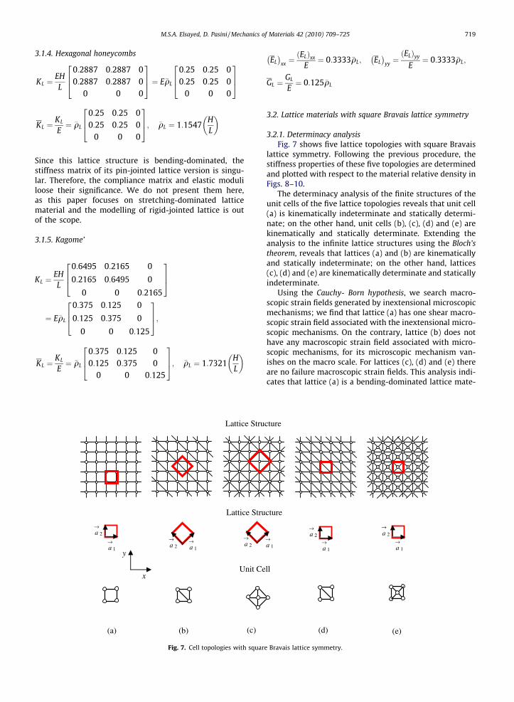
3.2.1. Determinacy analysisFig. 7 shows five lattice topologies with square Bravais

lattice symmetry. Following the previous procedure, thestiffness properties of these five topologies are determinedand plotted with respect to the material relative density inFigs. 8–10.

The determinacy analysis of the finite structures of theunit cells of the five lattice topologies reveals that unit cell(a) is kinematically indeterminate and statically determi-nate; on the other hand, unit cells (b), (c), (d) and (e) arekinematically and statically determinate. Extending theanalysis to the infinite lattice structures using the Bloch’stheorem, reveals that lattices (a) and (b) are kinematicallyand statically indeterminate; on the other hand, lattices(c), (d) and (e) are kinematically determinate and staticallyindeterminate.

Using the Cauchy- Born hypothesis, we search macro-scopic strain fields generated by inextensional microscopicmechanisms; we find that lattice (a) has one shear macro-scopic strain field associated with the inextensional micro-scopic mechanisms. On the contrary, lattice (b) does nothave any macroscopic strain field associated with micro-scopic mechanisms, for its microscopic mechanism van-ishes on the macro scale. For lattices (c), (d) and (e) thereare no failure macroscopic strain fields. This analysis indi-cates that lattice (a) is a bending-dominated lattice mate-

2

→a

1

→a

2

→a

1

→a1

→a

cture

cture

ll

(d) (e)

e Bravais lattice symmetry.

E⎜⎝⎛ −

LE⎠⎞−

xx

⎟⎠⎞

0.0

0

0.1

0

0.2

0

0.3

0

00

05

0.1

15

0.2

25

0.3

35

0.4

0 00.1 00.2 0.33 0.4

ρ0

L

−ρ0.5

L

0.6 0.77 0.8 00.9 1

Fig. 8. Relative Young’s modulus in the x-direction (see Figs. 4, 5, and 7) versus relative density of selected 2D lattice materials.

L

−ρ

yy

LE−

0 0.1 0.2 0.3 0.4 0.5 0.6 0.7 0.8 0.9 10

0.05

0.1

0.15

0.2

0.25

0.3

0.35

0.4

⎜⎝⎛

⎠⎞⎟⎠⎞

Fig. 9. Relative Young’s modulus in the y-direction (see Figs. 4, 5, and 7) versus relative density of selected 2D lattice materials.

720 M.S.A. Elsayed, D. Pasini / Mechanics of Materials 42 (2010) 709–725

rial and lattices (b), (c), (d) and (e) are stretching-domi-nated lattice materials.

3.2.2. Stiffness propertiesThe strain energy density is formulated and used to de-

rive the averaged stiffness properties of the five latticesshown in Fig. 7. The results are plotted with respect tothe relative density in Figs. 8–10.

Lattice (a)

KL ¼KL

E¼ �qL

0:5 0 00 0:5 00 0 0

264375; �qL ¼ 2

HL

� �

The computation of the compliance matrix and the elasticmoduli are not presented as the material is bending-dominated.

L−ρ

LG−

0 0.1 0.2 0.3 0.4 0.5 0.6 0.7 0.8 0.9 10

0.02

0.04

0.06

0.08

0.1

0.12

0.14

0.16

Fig. 10. Relative shear modulus versus relative density of selected 2D lattice materials.

M.S.A. Elsayed, D. Pasini / Mechanics of Materials 42 (2010) 709–725 721

Lattice (b)

KL¼KL

E¼ �qL

0:4347 0:0653 �0:0653

0:0653 0:4347 �0:0653

�0:0653 �0:0653 0:0653

26643775; �qL¼2:71

HL

� �

EL �

xx ¼ðELÞxx

E¼ 0:3694�qL; EL

�yy ¼

ðELÞyy

E¼ 0:3694�qL;

GL ¼GL

E¼ 0:0482�qL

Lattice (c)

KL ¼KL

E¼ �qL

0:3964 0:1036 0

0:1036 0:3964 0

0 0 0:1036

264375; �qL ¼ 3:41

HL

� �

EL �

xx ¼ðELÞxx

E¼ 0:3693�qL; EL

�yy ¼

ðELÞyy

E¼ 0:3693�qL;

GL ¼GL

E¼ 0:1036�qL

Lattice (d)

KL ¼KL

E¼ �qL

0:3964 0:1036 �0:1036

0:1036 0:3964 �0:1036

�0:1036 �0:1036 0:1036

26643775;

�qL ¼ 3:4142HL

� �

EL �

xx ¼ðELÞxx

E¼ 0:2928�qL; EL

�yy ¼

ðELÞyy

E¼ 0:2928�qL;

GL ¼GL

E¼ 0:0607�qL

Lattice (e)

KL ¼KL

E¼ �qL

0:3536 0:1464 0

0:1464 0:3536 0

0 0 0:1464

26643775; �qL¼4:8284

HL

� �

EL �

xx ¼ðELÞxx

E¼ 0:293�qL; EL

�yy ¼

ðELÞyy

E¼ 0:293�qL;

GL ¼GL

E¼ 0:1464�qL

4. Concluding remarks

This paper has described a systematic matrix-basedprocedure for the specific stiffness characterization of lat-tice materials with any arbitrary topology. This procedureis efficient for the automation of the characterization pro-cess of complex microscopic topologies. A scheme basedon the concept of dummy nodes has been introduced todeal with lattice materials that consist of unit cell elementsintersecting their cell envelopes. The procedure has beenapplied to lattice materials with hexagonal and squareBravais symmetries. The results have been plotted on de-sign charts that can help in the selection process of latticetopologies for given stiffness requirements. It is found thatthe lattice materials with cell topologies shown in Fig. 7band c exhibit 11% increase of the specific stiffness com-

722 M.S.A. Elsayed, D. Pasini / Mechanics of Materials 42 (2010) 709–725

pared to the Kagome’ and the full triangulation latticematerials. On the other hand, the lattice material with celltopology shown in Fig. 7e shows 17% improvement in thespecific shear modulus compared to the Kagome’ and thefull triangulation lattice materials.

Appendix A. The Dummy Node Scheme

Consider the sequence of three unit cells describingthe periodicity of the lattice structure shown in Fig. 11.We specify two elements, a and b, of lengths La and Lb.Element a is connected between node n1, located on theborders between unit cells I and II, and node n2 that be-longs to unit cell III. Element b is connected betweennode n3, belongs to unit cell I, and node n4 which belongsto unit cell II.

The envelope of unit cell II intersects elements a and b,respectively, at nodes n5 and n6, which are dummy nodesintroduced at intersection points between envelope andunit cell elements. Node n5 splits element a into two seg-ments a1 and a2 of length La1 and La2, respectively. On theother hand, node n6 divides element b into two segmentsb1 and b2 of length Lb1 and Lb2, respectively. Elements aand b carry internal tension forces ta and tb, respectively.Thus, the portions of the nodal forces that are in balancewith the tension forces in elements a and b are specifiedby a two dimensional vector fni that has two componentsin the x and the y-directions of the Cartesian coordinates.If r

!ni is the position vector of node ni and i 2

{1,2,3,4,5,6}, then a unit vector in the direction of ele-ments a and b can be written as:

na ¼r!

n5 � r!

n1

La1¼ r!

n2 � r!

n5

La2¼ r!

n2 � r!

n1

LaðA1Þ

nb ¼r!

n6 � r!

n3

Lb1¼ r!

n4 � r!

n6

Lb2¼ r!

n4 � r!

n3

LbðA2Þ

A.1. Equilibrium analysis

The static equilibrium system of a structure that has belements connected between j nodes is represented as:

Fig. 11. Lattice structure (left) and zoom on three unit cells (right) tessellated in tstructural elements; dashed lines: cell envelopes; s: real structural nodes; j: d

At ¼ f ðA3Þ

where A 2 Rnj�b, n = 2 in 2D, is a Jacobian matrix with en-tries of direction cosines that transforms the vector of ten-sion forces of the structural elements t 2 Rb to the vector ofthe nodal forces f 2 Rnj(Kuznetsov, 2000; Kuznetsov, 1997).

Consider the segment a1 of element a; the static equi-librium of forces at nodes n1 and n5 with the tension forcein the element ta can be written as:

�na

na

� �ta ¼

fn1

fn5

� �ðA4Þ

Similarly, consider the segment a2 of element a, the staticequilibrium of forces at nodes n5 and n2 with the tensionforce in the element ta is given by:

�na

na

� �ta ¼

fn5

fn2

� �ðA5Þ

The assembly of Eqs. (A4) and (A5) into one matrix systemresults in:

�na

na � na

na

2666637777ta ¼

�na

0na

2666637777ta ¼

fn1

fn5

fn2

2666637777 ðA6Þ

From Eq. (A6) one can realize that the coefficients of thedummy node, n5, can be set to zero to eliminate the nodefrom the matrix system, which results in:

�na

na

� �ta ¼

fn1

fn2

� �ðA7Þ

The same reasoning can be applied to element b, where theequilibrium of the nodal forces at nodes n3, n4 and n6 withthe element tension force tb can be expressed, respectively,in Eqs. (A8) and (A9) as:

�nb

nb

� �tb ¼

fn3

fn6

� �ðA8Þ

�nb

nb

� �tb ¼

fn6

fn4

� �ðA9Þ

he direction of the horizontal translational basis. Legend: Continuous lines:ummy nodes.

M.S.A. Elsayed, D. Pasini / Mechanics of Materials 42 (2010) 709–725 723

The assembly of Eqs. (A8) and (A9) in one matrix systemresults in:

�nb

nb

� �tb ¼

fn3

fn4

� �ðA10Þ

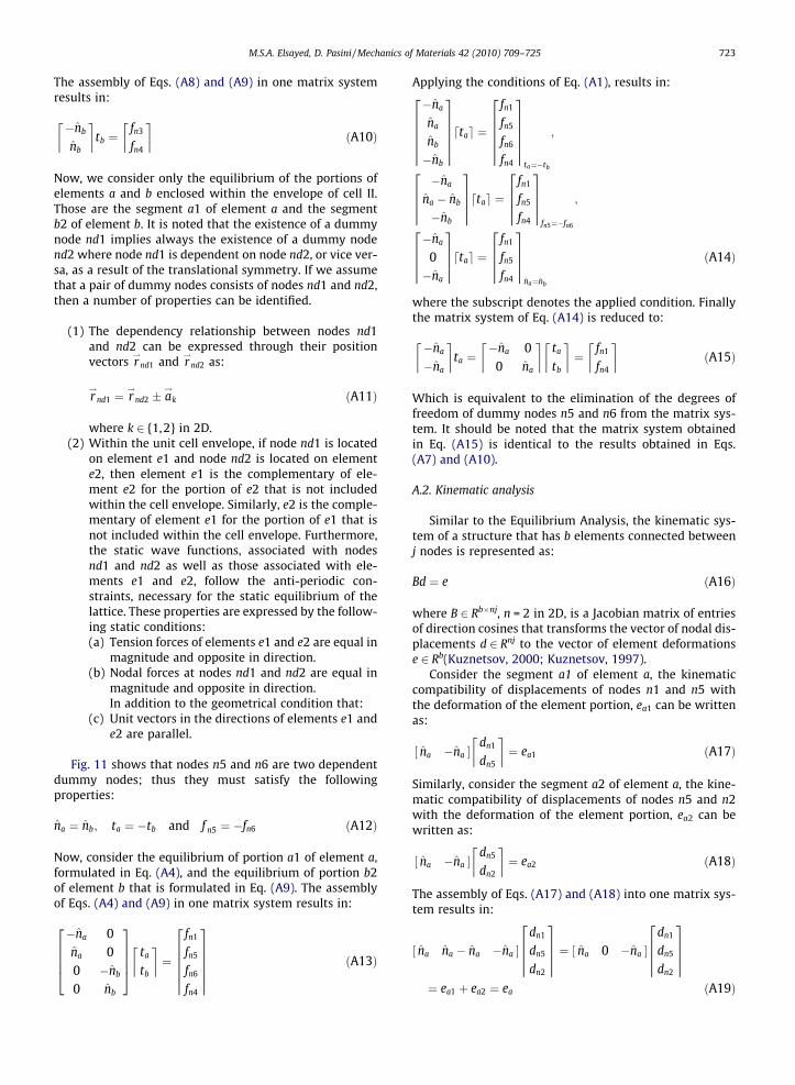
Now, we consider only the equilibrium of the portions ofelements a and b enclosed within the envelope of cell II.Those are the segment a1 of element a and the segmentb2 of element b. It is noted that the existence of a dummynode nd1 implies always the existence of a dummy nodend2 where node nd1 is dependent on node nd2, or vice ver-sa, as a result of the translational symmetry. If we assumethat a pair of dummy nodes consists of nodes nd1 and nd2,then a number of properties can be identified.

(1) The dependency relationship between nodes nd1and nd2 can be expressed through their positionvectors r

!nd1 and r

!nd2 as:

r!

nd1 ¼ r!

nd2 a!

k ðA11Þ

where k 2 {1,2} in 2D.

(2) Within the unit cell envelope, if node nd1 is located

on element e1 and node nd2 is located on elemente2, then element e1 is the complementary of ele-ment e2 for the portion of e2 that is not includedwithin the cell envelope. Similarly, e2 is the comple-mentary of element e1 for the portion of e1 that isnot included within the cell envelope. Furthermore,the static wave functions, associated with nodesnd1 and nd2 as well as those associated with ele-ments e1 and e2, follow the anti-periodic con-straints, necessary for the static equilibrium of thelattice. These properties are expressed by the follow-ing static conditions:

(a) Tension forces of elements e1 and e2 are equal in

magnitude and opposite in direction.(b) Nodal forces at nodes nd1 and nd2 are equal in

magnitude and opposite in direction.In addition to the geometrical condition that:

(c) Unit vectors in the directions of elements e1 ande2 are parallel.

Fig. 11 shows that nodes n5 and n6 are two dependentdummy nodes; thus they must satisfy the followingproperties:

na ¼ nb; ta ¼ �tb and f n5 ¼ �fn6 ðA12Þ

Now, consider the equilibrium of portion a1 of element a,formulated in Eq. (A4), and the equilibrium of portion b2of element b that is formulated in Eq. (A9). The assemblyof Eqs. (A4) and (A9) in one matrix system results in:

�na 0na 00 �nb

0 nb

2666437775 ta

tb

� �¼

fn1

fn5

fn6

fn4

2666666

3777777 ðA13Þ

Applying the conditions of Eq. (A1), results in:

�na

na

nb

�nb

2666666

3777777 tad e ¼

fn1

fn5

fn6

fn4

2666666

3777777ta¼�tb

;

�na

na � nb

�nb

2666637777 tad e ¼

fn1

fn5

fn4

2666637777

fn5¼�fn6

;

�na

0�na

2666637777 tad e ¼

fn1

fn5

fn4

2666637777

na¼nb

ðA14Þ

where the subscript denotes the applied condition. Finallythe matrix system of Eq. (A14) is reduced to:

�na

�na

� �ta ¼

�na 00 na

� �ta

tb

� �¼

fn1

fn4

� �ðA15Þ

Which is equivalent to the elimination of the degrees offreedom of dummy nodes n5 and n6 from the matrix sys-tem. It should be noted that the matrix system obtainedin Eq. (A15) is identical to the results obtained in Eqs.(A7) and (A10).

A.2. Kinematic analysis

Similar to the Equilibrium Analysis, the kinematic sys-tem of a structure that has b elements connected betweenj nodes is represented as:

Bd ¼ e ðA16Þ

where B 2 Rb�nj, n = 2 in 2D, is a Jacobian matrix of entriesof direction cosines that transforms the vector of nodal dis-placements d 2 Rnj to the vector of element deformationse 2 Rb(Kuznetsov, 2000; Kuznetsov, 1997).

Consider the segment a1 of element a, the kinematiccompatibility of displacements of nodes n1 and n5 withthe deformation of the element portion, ea1 can be writtenas:

na �na½ �dn1

dn5

� �¼ ea1 ðA17Þ

Similarly, consider the segment a2 of element a, the kine-matic compatibility of displacements of nodes n5 and n2with the deformation of the element portion, ea2 can bewritten as:

na �na½ �dn5

dn2

� �¼ ea2 ðA18Þ

The assembly of Eqs. (A17) and (A18) into one matrix sys-tem results in:

na na � na �na½ �dn1

dn5

dn2

2666637777 ¼ na 0 �na½ �

dn1

dn5

dn2

2666637777

¼ ea1 þ ea2 ¼ ea ðA19Þ

724 M.S.A. Elsayed, D. Pasini / Mechanics of Materials 42 (2010) 709–725

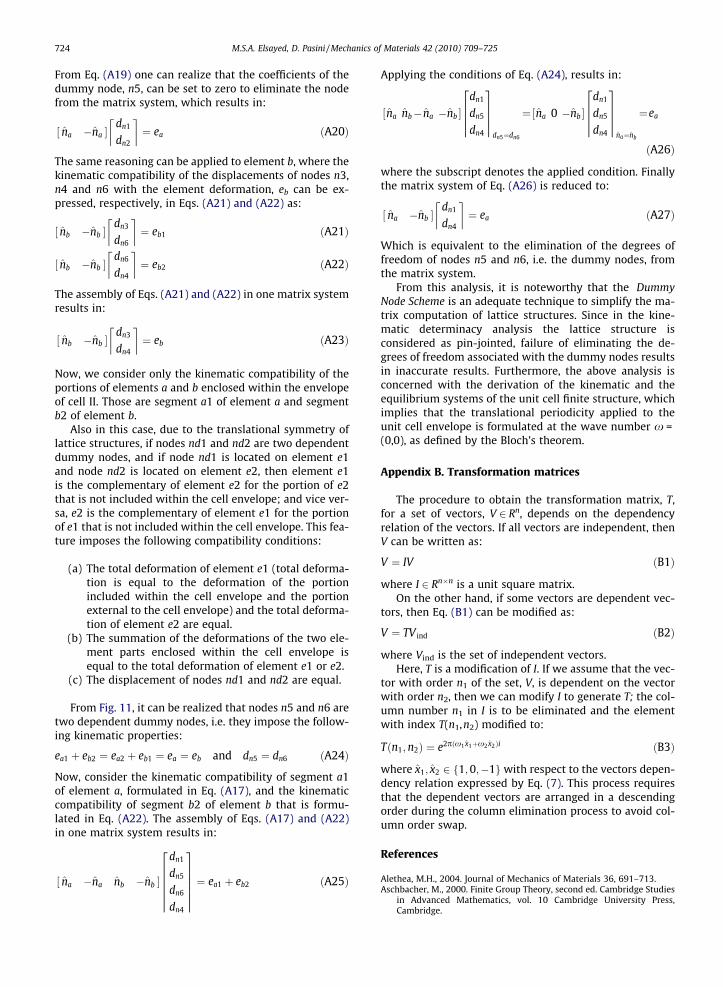
From Eq. (A19) one can realize that the coefficients of thedummy node, n5, can be set to zero to eliminate the nodefrom the matrix system, which results in:

na �na½ �dn1

dn2

� �¼ ea ðA20Þ

The same reasoning can be applied to element b, where thekinematic compatibility of the displacements of nodes n3,n4 and n6 with the element deformation, eb can be ex-pressed, respectively, in Eqs. (A21) and (A22) as:

nb �nb½ �dn3

dn6

� �¼ eb1 ðA21Þ

nb �nb½ �dn6

dn4

� �¼ eb2 ðA22Þ

The assembly of Eqs. (A21) and (A22) in one matrix systemresults in:

nb �nb½ �dn3

dn4

� �¼ eb ðA23Þ

Now, we consider only the kinematic compatibility of theportions of elements a and b enclosed within the envelopeof cell II. Those are segment a1 of element a and segmentb2 of element b.

Also in this case, due to the translational symmetry oflattice structures, if nodes nd1 and nd2 are two dependentdummy nodes, and if node nd1 is located on element e1and node nd2 is located on element e2, then element e1is the complementary of element e2 for the portion of e2that is not included within the cell envelope; and vice ver-sa, e2 is the complementary of element e1 for the portionof e1 that is not included within the cell envelope. This fea-ture imposes the following compatibility conditions:

(a) The total deformation of element e1 (total deforma-tion is equal to the deformation of the portionincluded within the cell envelope and the portionexternal to the cell envelope) and the total deforma-tion of element e2 are equal.

(b) The summation of the deformations of the two ele-ment parts enclosed within the cell envelope isequal to the total deformation of element e1 or e2.

(c) The displacement of nodes nd1 and nd2 are equal.

From Fig. 11, it can be realized that nodes n5 and n6 aretwo dependent dummy nodes, i.e. they impose the follow-ing kinematic properties:

ea1 þ eb2 ¼ ea2 þ eb1 ¼ ea ¼ eb and dn5 ¼ dn6 ðA24Þ

Now, consider the kinematic compatibility of segment a1of element a, formulated in Eq. (A17), and the kinematiccompatibility of segment b2 of element b that is formu-lated in Eq. (A22). The assembly of Eqs. (A17) and (A22)in one matrix system results in:

na �na nb �nb½ �

dn1

dn5

dn6

dn4

2666666

3777777 ¼ ea1 þ eb2 ðA25Þ

Applying the conditions of Eq. (A24), results in:

na nb� na �nb½ �dn1

dn5

dn4

2666637777

dn5¼dn6

¼ na 0 �nb½ �dn1

dn5

dn4

2666637777

na¼nb

¼ea

ðA26Þ

where the subscript denotes the applied condition. Finallythe matrix system of Eq. (A26) is reduced to:

na �nb½ �dn1

dn4

� �¼ ea ðA27Þ

Which is equivalent to the elimination of the degrees offreedom of nodes n5 and n6, i.e. the dummy nodes, fromthe matrix system.

From this analysis, it is noteworthy that the DummyNode Scheme is an adequate technique to simplify the ma-trix computation of lattice structures. Since in the kine-matic determinacy analysis the lattice structure isconsidered as pin-jointed, failure of eliminating the de-grees of freedom associated with the dummy nodes resultsin inaccurate results. Furthermore, the above analysis isconcerned with the derivation of the kinematic and theequilibrium systems of the unit cell finite structure, whichimplies that the translational periodicity applied to theunit cell envelope is formulated at the wave number x =(0,0), as defined by the Bloch’s theorem.

Appendix B. Transformation matrices

The procedure to obtain the transformation matrix, T,for a set of vectors, V 2 Rn, depends on the dependencyrelation of the vectors. If all vectors are independent, thenV can be written as:

V ¼ IV ðB1Þ

where I 2 Rn�n is a unit square matrix.On the other hand, if some vectors are dependent vec-

tors, then Eq. (B1) can be modified as:

V ¼ TV ind ðB2Þ

where Vind is the set of independent vectors.Here, T is a modification of I. If we assume that the vec-

tor with order n1 of the set, V, is dependent on the vectorwith order n2, then we can modify I to generate T; the col-umn number n1 in I is to be eliminated and the elementwith index T(n1,n2) modified to:

Tðn1; n2Þ ¼ e2p x1 x1þx2 x2ð Þi ðB3Þ

where x1; x2 2 f1;0;�1gwith respect to the vectors depen-dency relation expressed by Eq. (7). This process requiresthat the dependent vectors are arranged in a descendingorder during the column elimination process to avoid col-umn order swap.

References

Alethea, M.H., 2004. Journal of Mechanics of Materials 36, 691–713.Aschbacher, M., 2000. Finite Group Theory, second ed. Cambridge Studies

in Advanced Mathematics, vol. 10 Cambridge University Press,Cambridge.

M.S.A. Elsayed, D. Pasini / Mechanics of Materials 42 (2010) 709–725 725

Bhattacharya, K., 2003. Microstructure of Martensite: Why it Forms andHow it Gives Rise to the Shape-Memory Effect. Oxford Series onMaterials Modeling, vol. 2. Oxford University Press, New York.

Born, M., Huang, K., 1954. Dynamical Theory of Crystal Lattices. ClarendonPress, Oxford.

Brillouin, L., 1946. Wave Propagation in Periodic Structures, InternationalSeries in Pure and Applied Physics. McGraw-Hill, New York.

Brillouin, L., 1953. Wave Propagation in Periodic Structures, second ed.Dover, New York.

Calladine, C.R., 1978. International Journal of Solids and Structures 14,161–172.

Deshpande, V.S., Ashby, M.F., Fleck, N.A., 2001. Acta Materialia 49 (6),1035–1040.

Ericksen, J.L., 1984. In: Gurtin, M.E. (Ed.), Phase Transformations andMaterial Instabilities in Solids. Academic Press, New York.

Gibson, L.J., Ashby, M.F., 1997. Cellular Solids: Structure and Properties.second ed. Cambridge University Press, Cambridge.

Grosso, G., Pastori-Parravincini, G., 2000. Solid State Physics. AcademicPress, London.

Hill, V.E., 2000. Groups and Characters. Chapman & Hall/CRC Press, BocaRaton, FL.

Horn, Roger A., Johnson, Charles R., 1985. Matrix Analysis. CambridgeUniversity Press, Cambridge.

Horn, Roger A., Johnson, Charles R., 1991. Topics in Matrix Analysis.Cambridge University Press, Cambridge.

Hutchinson, R.G., 2004. Mechanics of Lattice Materials. Ph.D. Thesis,Cambridge University, Cambridge.

Hutchinson, R.G., Fleck, N.A., 2006. Journal of the Mechanics and Physicsof Solids 54 (4), 756–782.

James, G., Liebeck, M., 2001. Representations and Characters of Groups.second ed. Cambridge University Press, Cambridge.

Jones, W., March, N.H., 1973. Theoretical Solid State Physics. vol. 1, Wiley–Interscience, London.

Kuznetsov, E.N., 1997. International Journal of Solids and Structures 34,3657–3671.

Kuznetsov, E.N., 2000. International Journal of Solids and Structures 37(15), 2215–2223.

Langley, R.S., 1993. Journal of Sound and Vibration 167, 377–381.Langley, R.S., Bardell, N.S., Ruivo, H.M., 1997. Journal of Sound and

Vibration 207, 521–535.Maugin, G.A., 1992. The Thermomechanics of Plasticity and Fracture.

Cambridge Texts in Applied Mathematics. Cambridge UniversityPress, Cambridge.

Maxwell, J.C., 1864. Philosophical Magazine, 27, 294, 1864, Paper XXVI inCollected papers, Cambridge 1890.

Pellegrino, S., 1993. International Journal of Solids and Structures 34 (21),2035–3025.

Pellegrino, S., Calladine, C.R., 1986. International Journal of Solids andStructures 22 (4), 409–428.

Phani, S.A., Woodhouse, J., Fleck, N.A., 2006. Journal of the AcousticalSociety of America 119 (4), 1995–2005.

Pitteri, M., Zanzotto, G., 2003. Continuum Models for Phase Transitionsand Twinning in Crystals. Chapman & Hall/CRC Press, Boca Raton, FL.

Renton, J.D., 2002. Elastic Beams and Frames, second ed. HorwoodPublishing Limited, England.

Strang, G., 1988. Linear Algebra and Its Applications, third ed. Wellesley–Cambridge Press, Cambridge.