www.iap.uni-jena.de

Medical Photonics Lecture

Optical Engineering

Lecture 6: Aberrations

2017-11-30

Herbert Gross

Winter term 2017

2

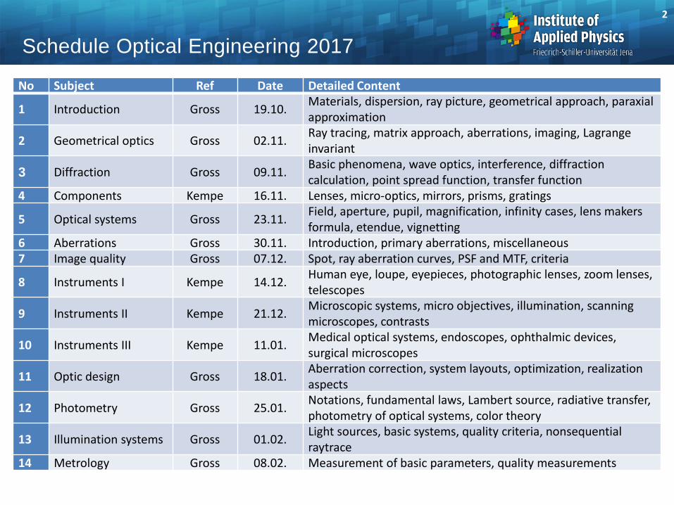
Schedule Optical Engineering 2017

No Subject Ref Date Detailed Content

1 Introduction Gross 19.10. Materials, dispersion, ray picture, geometrical approach, paraxial approximation

2 Geometrical optics Gross 02.11. Ray tracing, matrix approach, aberrations, imaging, Lagrange invariant

3 Diffraction Gross 09.11. Basic phenomena, wave optics, interference, diffraction calculation, point spread function, transfer function

4 Components Kempe 16.11. Lenses, micro-optics, mirrors, prisms, gratings

5 Optical systems Gross 23.11. Field, aperture, pupil, magnification, infinity cases, lens makers formula, etendue, vignetting

6 Aberrations Gross 30.11. Introduction, primary aberrations, miscellaneous 7 Image quality Gross 07.12. Spot, ray aberration curves, PSF and MTF, criteria

8 Instruments I Kempe 14.12. Human eye, loupe, eyepieces, photographic lenses, zoom lenses, telescopes

9 Instruments II Kempe 21.12. Microscopic systems, micro objectives, illumination, scanning microscopes, contrasts

10 Instruments III Kempe 11.01. Medical optical systems, endoscopes, ophthalmic devices, surgical microscopes

11 Optic design Gross 18.01. Aberration correction, system layouts, optimization, realization aspects

12 Photometry Gross 25.01. Notations, fundamental laws, Lambert source, radiative transfer, photometry of optical systems, color theory

13 Illumination systems Gross 01.02. Light sources, basic systems, quality criteria, nonsequential raytrace

14 Metrology Gross 08.02. Measurement of basic parameters, quality measurements

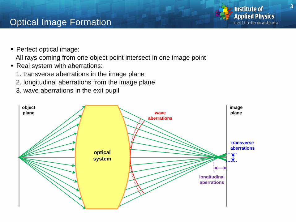
Optical Image Formation

optical

system

object

plane

image

plane

transverse

aberrations

longitudinal

aberrations

wave

aberrations

Perfect optical image:

All rays coming from one object point intersect in one image point

Real system with aberrations:

1. transverse aberrations in the image plane

2. longitudinal aberrations from the image plane

3. wave aberrations in the exit pupil

3

Longitudinal aberrations Ds

Transverse aberrations Dy

Representation of Geometrical Aberrations

Gaussian image

plane

ray

longitudinal

aberration

D s'

optical axis

system

U'reference

point

reference

plane

reference ray

(real or ideal chief ray)

transverse

aberrationDy'

optical axis

system

ray

U'

Gaussian

image

plane

reference ray

longitudinal aberration

projected on the axis

Dl'

optical axis

system

ray

Dl'o

logitudinal aberration

along the reference ray

4

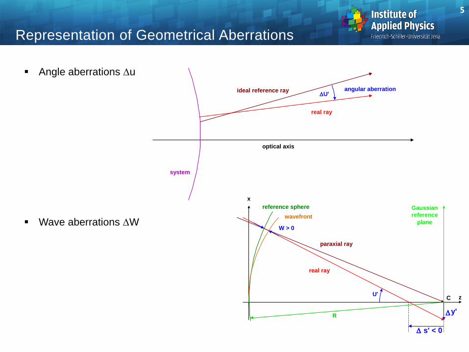
Representation of Geometrical Aberrations

ideal reference ray angular aberrationDU'

optical axis

system

real ray

x

z

s' < 0D

W > 0

reference sphere

paraxial ray

real ray

wavefront

R

C

y'D

Gaussian

reference

plane

U'

Angle aberrations Du

Wave aberrations DW

5

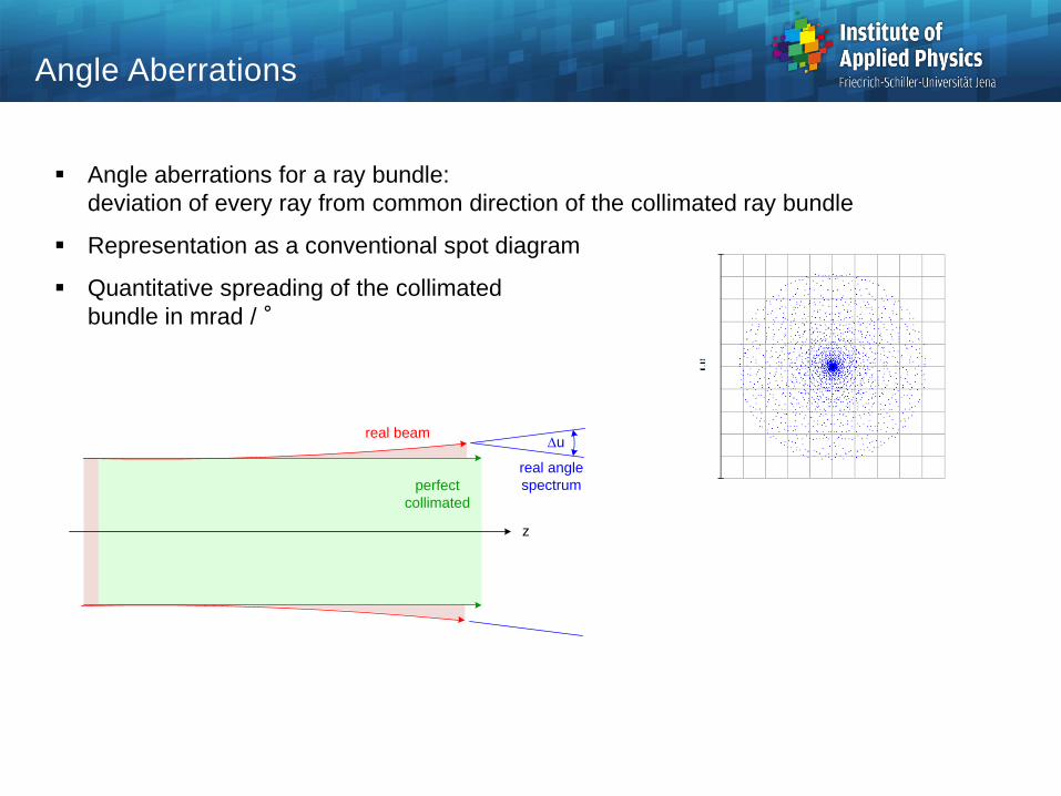
Angle Aberrations

Angle aberrations for a ray bundle:

deviation of every ray from common direction of the collimated ray bundle

Representation as a conventional spot diagram

Quantitative spreading of the collimated

bundle in mrad / °

perfect

collimated

real angle

spectrum

real beamDu

z

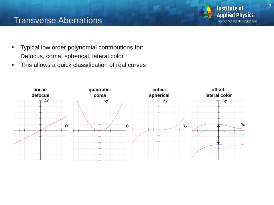
Transverse Aberrations

Typical low order polynomial contributions for:

Defocus, coma, spherical, lateral color

This allows a quick classification of real curves

linear:

defocus

quadratic:

coma

cubic:

spherical

offset:

lateral colorDy DyDyDy

ypypypyp

7

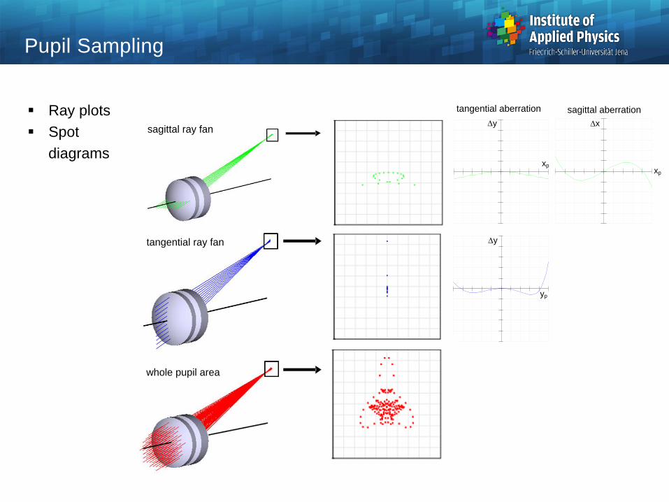
Pupil Sampling

Ray plots

Spot

diagrams

sagittal ray fan

tangential ray fan

yp

Dy

tangential aberration

xp

Dy

xp

Dx

sagittal aberration

whole pupil area

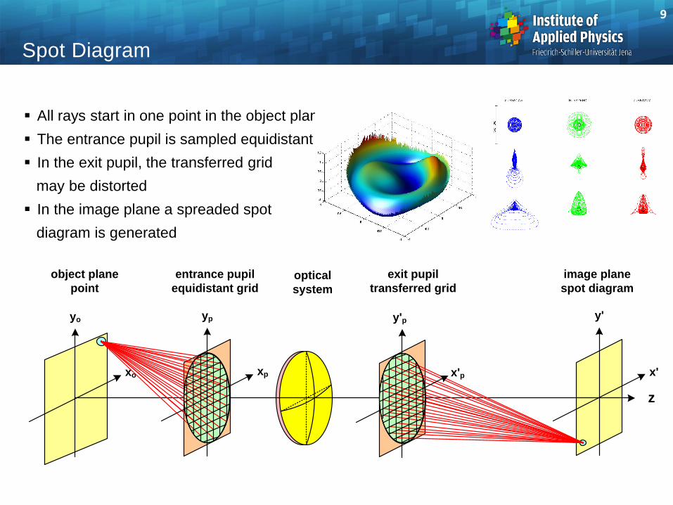
Spot Diagram

y'p

x'p

yp

xp x'

y'

z

yo

xo

object plane

point

entrance pupil

equidistant grid

exit pupil

transferred grid

image plane

spot diagramoptical

system

All rays start in one point in the object plane

The entrance pupil is sampled equidistant

In the exit pupil, the transferred grid

may be distorted

In the image plane a spreaded spot

diagram is generated

9

Dmlk

ml

p

k

klmp ryaryy,,

cos'),,'(

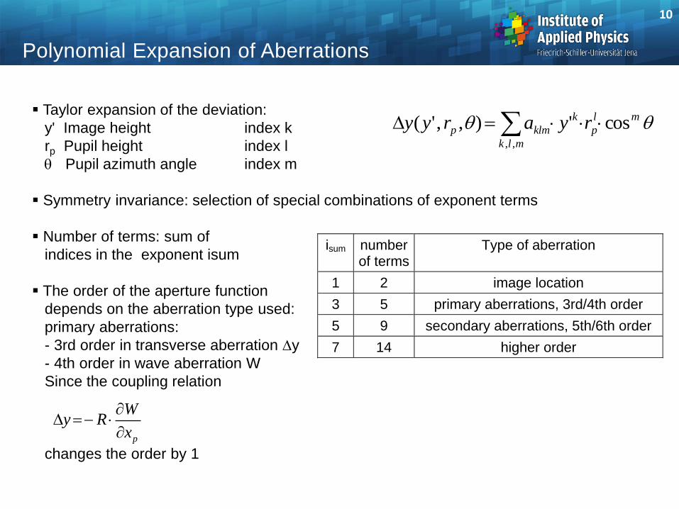
Polynomial Expansion of Aberrations

Taylor expansion of the deviation:

y' Image height index k

rp Pupil height index l

Pupil azimuth angle index m

Symmetry invariance: selection of special combinations of exponent terms

Number of terms: sum of

indices in the exponent isum

The order of the aperture function

depends on the aberration type used:

primary aberrations:

- 3rd order in transverse aberration Dy

- 4th order in wave aberration W

Since the coupling relation

changes the order by 1

10

p

Wy R

x

D

isum number of terms

Type of aberration

1 2 image location

3 5 primary aberrations, 3rd/4th order

5 9 secondary aberrations, 5th/6th order

7 14 higher order

Polynomial Expansion of Aberrations

Representation of 2-dimensional Taylor series vs field y and aperture r

Selection rules: checkerboard filling of the matrix

Constant sum of exponents according to the order

Field y

Spherical

y0 y 1 y 2 y3 y 4 y 5

Distortion

r

0

y

y3

primary

y5

secondary

r

1

r 1

Defocus

Aper-

ture

r

r

2

r2y Coma primary

r 3

r 3 Spherical

primary

r

4

r

5

r 5 Spherical

secondary

DistortionDistortionTilt

Coma Astigmatism

Image

location

Primary

aberrations /

Seidel

Astig./Curvat.

cos

cos

cos2

cos

Secondary

aberrations

cos

r 3y 2 cos

2

Coma

secondary

r4y cos

r2y

3 cos

3

r2y

3 cos

r1 y

4

r1 y

4 cos

2

r 3y 2

r12

yr 12

y

p

p

p

p

p

p

p

p

p

p

p

p

p

p

p

p

p

p

p

p

11

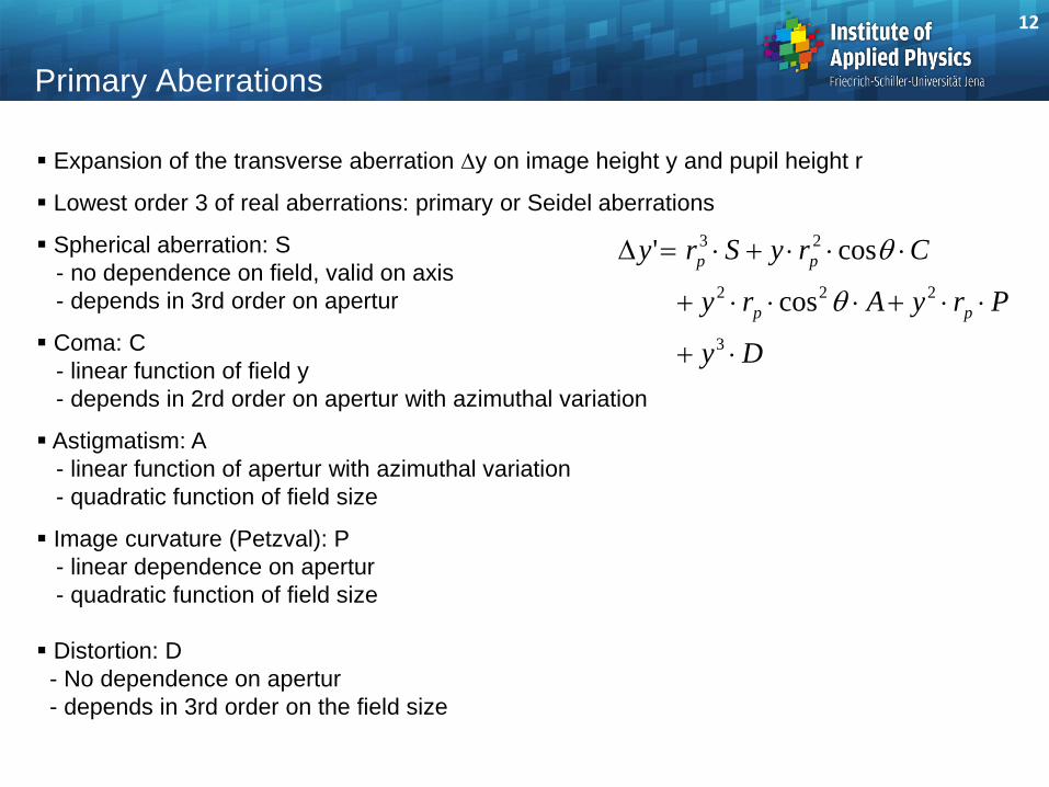
Primary Aberrations

Dy

PryAry

CrySry

pp

pp

D

3

222

23

cos

cos'

Expansion of the transverse aberration Dy on image height y and pupil height r

Lowest order 3 of real aberrations: primary or Seidel aberrations

Spherical aberration: S

- no dependence on field, valid on axis

- depends in 3rd order on apertur

Coma: C

- linear function of field y

- depends in 2rd order on apertur with azimuthal variation

Astigmatism: A

- linear function of apertur with azimuthal variation

- quadratic function of field size

Image curvature (Petzval): P

- linear dependence on apertur

- quadratic function of field size

Distortion: D

- No dependence on apertur

- depends in 3rd order on the field size

12

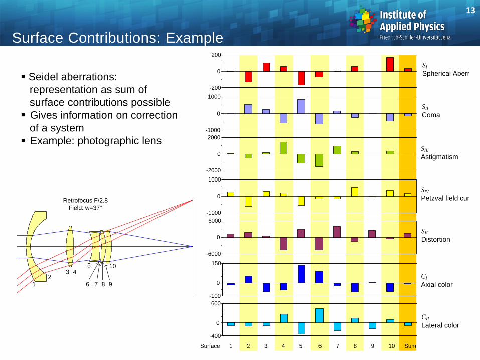
Surface Contributions: Example

13

Seidel aberrations:

representation as sum of

surface contributions possible

Gives information on correction

of a system

Example: photographic lens

1

23 4

5

6 8 9

10

7

Retrofocus F/2.8

Field: w=37°

SI

Spherical Aberration

SII

Coma

-200

0

200

-1000

0

1000

-2000

0

2000

-1000

0

1000

-100

0

150

-400

0

600

-6000

0

6000

SIII

Astigmatism

SIV

Petzval field curvature

SV

Distortion

CI

Axial color

CII

Lateral color

Surface 1 2 3 4 5 6 7 8 9 10 Sum

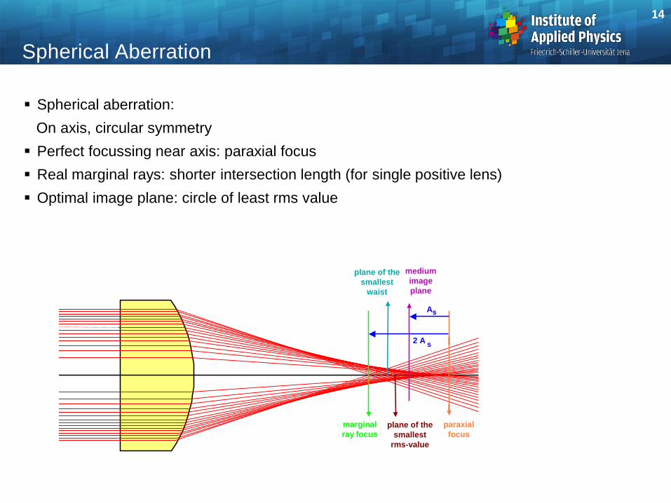
Spherical Aberration

Spherical aberration:

On axis, circular symmetry

Perfect focussing near axis: paraxial focus

Real marginal rays: shorter intersection length (for single positive lens)

Optimal image plane: circle of least rms value

paraxial

focus

marginal

ray focusplane of the

smallest

rms-value

medium

image

plane

As

plane of the

smallest

waist

2 A s

14

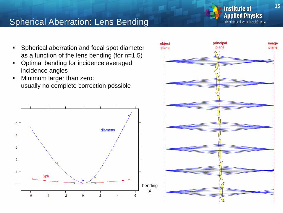
Spherical aberration and focal spot diameter

as a function of the lens bending (for n=1.5)

Optimal bending for incidence averaged

incidence angles

Minimum larger than zero:

usually no complete correction possible

Spherical Aberration: Lens Bending

object

plane

image

plane

principal

plane

15

diameter

bending

X

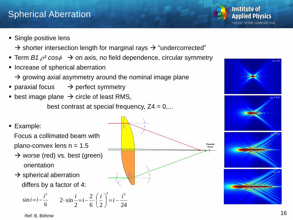
Spherical Aberration

16

Single positive lens

shorter intersection length for marginal rays “undercorrected”

Term B1 r³ cosf on axis, no field dependence, circular symmetry

Increase of spherical aberration

growing axial asymmetry around the nominal image plane

paraxial focus perfect symmetry

best image plane circle of least RMS,

best contrast at special frequency, Z4 = 0,...

Example:

Focus a collimated beam with

plano-convex lens n = 1.5

worse (red) vs. best (green)

orientation

spherical aberration

differs by a factor of 4:

c9 = 0

c9 = 0.3

c9 = 0.7

c9 = 1

i

i1

i2

Paraxial

focus

6sin

3iii

2426

2

2sin2

33i

ii

ii

Ref: B. Böhme

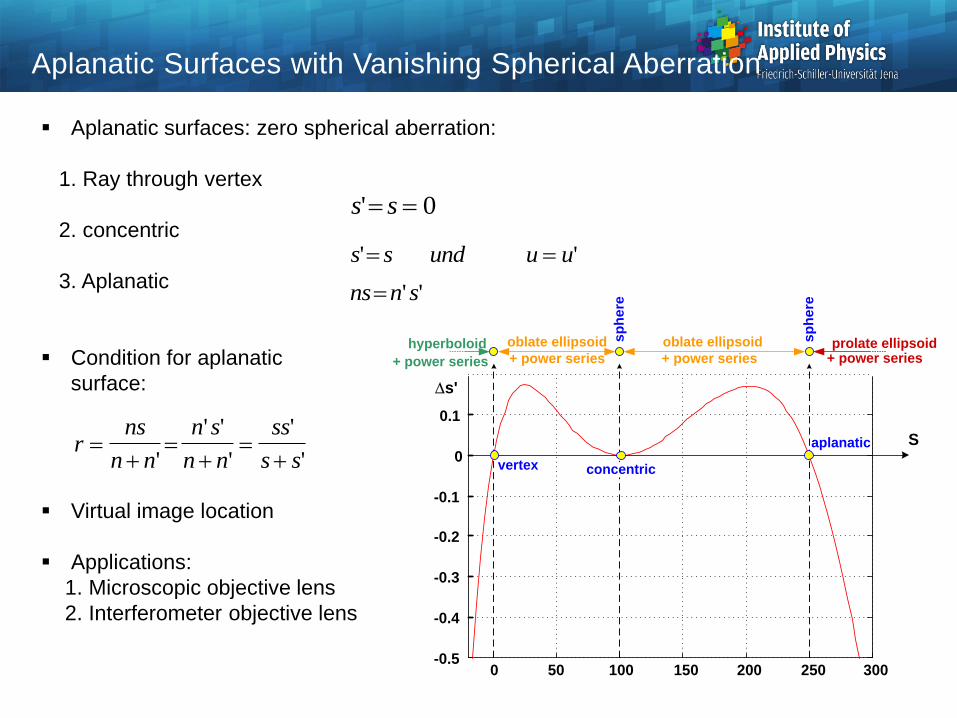
Aplanatic Surfaces with Vanishing Spherical Aberration

Ds'

0 50 100 150 200 250 300-0.5

-0.4

-0.3

-0.2

-0.1

0

0.1

Saplanatic

concentricvertex

oblate ellipsoidoblate ellipsoid prolate ellipsoidhyperboloid+ power series + power series+ power series + power series

sp

he

re

sp

he

re

Aplanatic surfaces: zero spherical aberration:

1. Ray through vertex

2. concentric

3. Aplanatic

Condition for aplanatic

surface:

Virtual image location

Applications:

1. Microscopic objective lens

2. Interferometer objective lens

s s und u u' '

s s' 0

ns n s ' '

rns

n n

n s

n n

ss

s s

'

' '

'

'

'

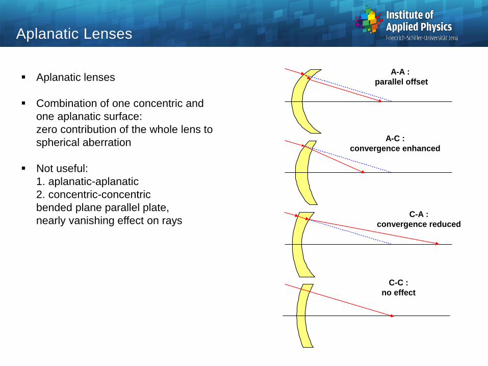
Aplanatic lenses

Combination of one concentric and

one aplanatic surface:

zero contribution of the whole lens to

spherical aberration

Not useful:

1. aplanatic-aplanatic

2. concentric-concentric

bended plane parallel plate,

nearly vanishing effect on rays

Aplanatic Lenses

A-A :

parallel offset

A-C :

convergence enhanced

C-C :

no effect

C-A :

convergence reduced

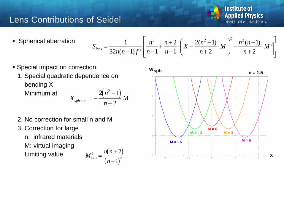
Lens Contributions of Seidel

Spherical aberration

Special impact on correction:

1. Special quadratic dependence on

bending X

Minimum at

2. No correction for small n and M

3. Correction for large

n: infrared materials

M: virtual imaging

Limiting value

2

22

23

3 2

)1(

2

)1(2

1

2

1)1(32

1M

n

nnM

n

nX

n

n

n

n

fnnSlens

sphW

X

M = 6M = - 6

M = - 3M = 0

M = 3

n = 1.5

X

n

nMsph min

2 1

2

2

M

n n

ns

0

2

2

2

1

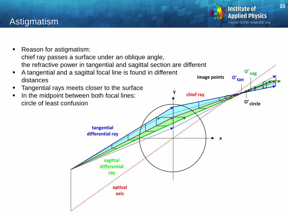
Reason for astigmatism:

chief ray passes a surface under an oblique angle,

the refractive power in tangential and sagittal section are different

A tangential and a sagittal focal line is found in different

distances

Tangential rays meets closer to the surface

In the midpoint between both focal lines:

circle of least confusion

Astigmatism

20

O'tansagO'

optical axis

chief ray

tangentialdifferential ray

sagittaldifferential

ray

y

x

O'circle

image points

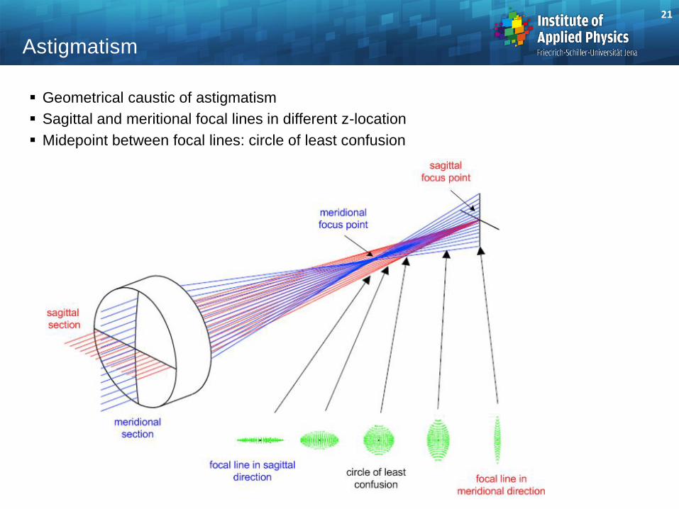
Geometrical caustic of astigmatism

Sagittal and meritional focal lines in different z-location

Midepoint between focal lines: circle of least confusion

21

Astigmatism

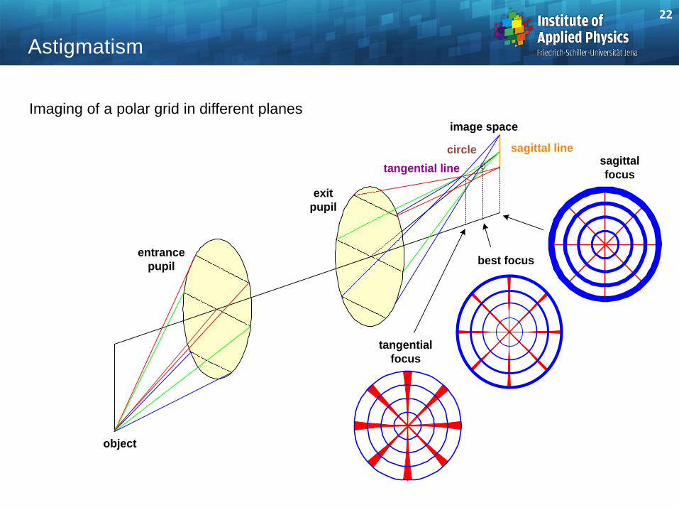
Imaging of a polar grid in different planes

sagittal line

tangential line

entrance

pupil

exit

pupil

object

circlesagittal

focus

tangential

focus

best focus

image space

Astigmatism

22

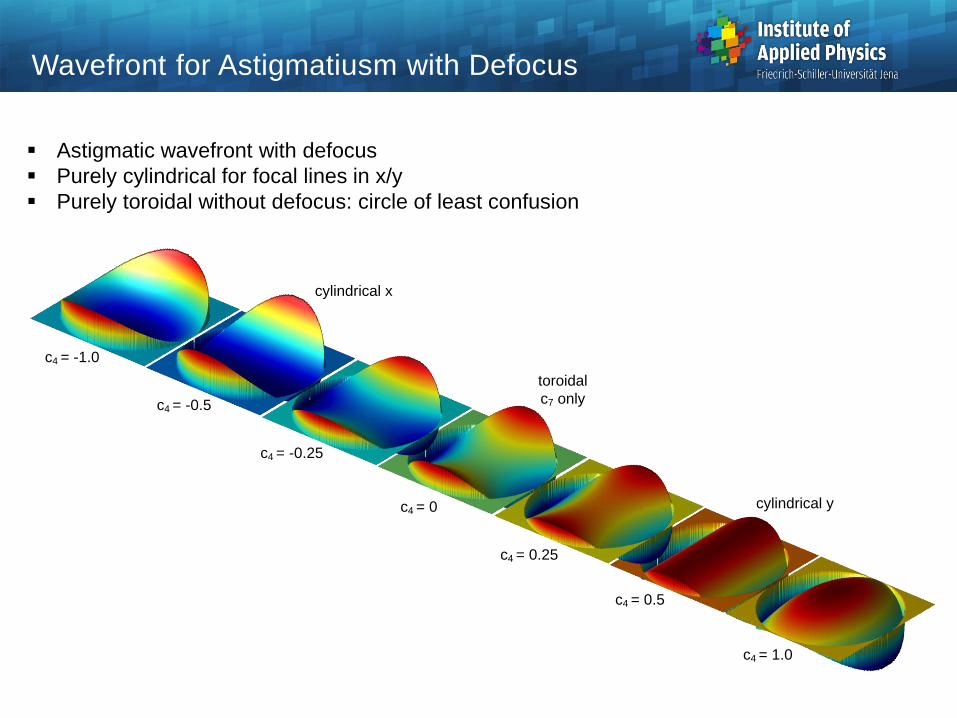
Wavefront for Astigmatiusm with Defocus

Astigmatic wavefront with defocus

Purely cylindrical for focal lines in x/y

Purely toroidal without defocus: circle of least confusion

c4 = 0

toroidal

c7 only

c4 = 0.25

c4 = 1.0

c4 = 0.5

c4 = -0.25

c4 = -1.0

c4 = -0.5

cylindrical x

cylindrical y

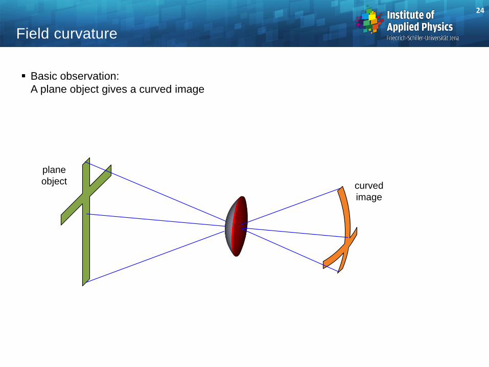
Basic observation:

A plane object gives a curved image

24

Field curvature

plane

object curved

image

ideal

image

plane

tangential

shell

sagittal

shell

image surfacesy'

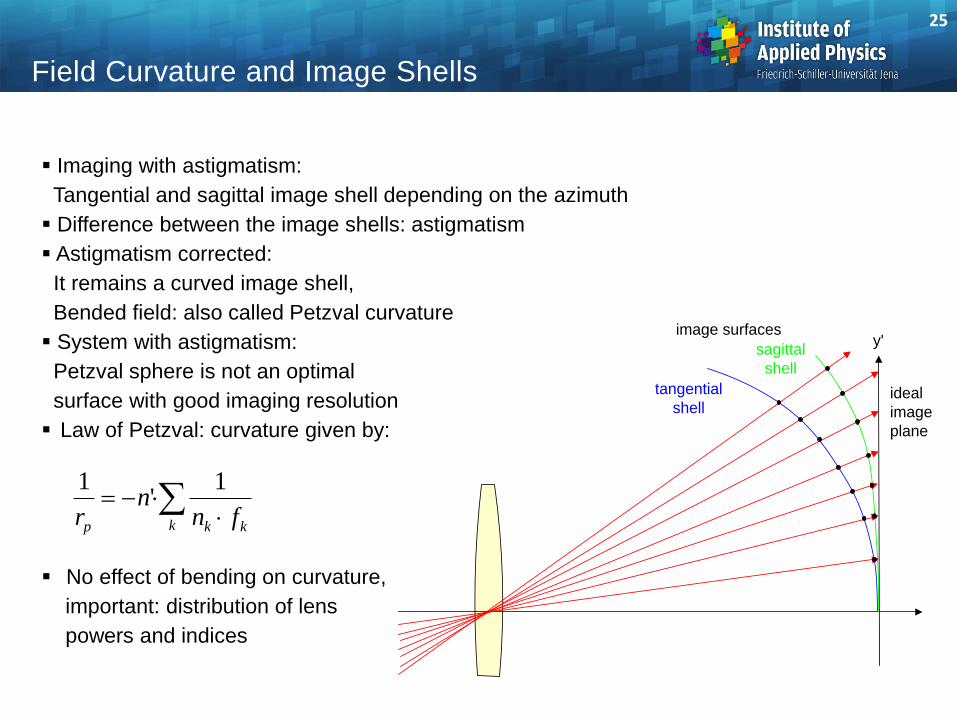
Field Curvature and Image Shells

Imaging with astigmatism:

Tangential and sagittal image shell depending on the azimuth

Difference between the image shells: astigmatism

Astigmatism corrected:

It remains a curved image shell,

Bended field: also called Petzval curvature

System with astigmatism:

Petzval sphere is not an optimal

surface with good imaging resolution

Law of Petzval: curvature given by:

No effect of bending on curvature,

important: distribution of lens

powers and indices

1 1

rn

n fp k kk

'

25

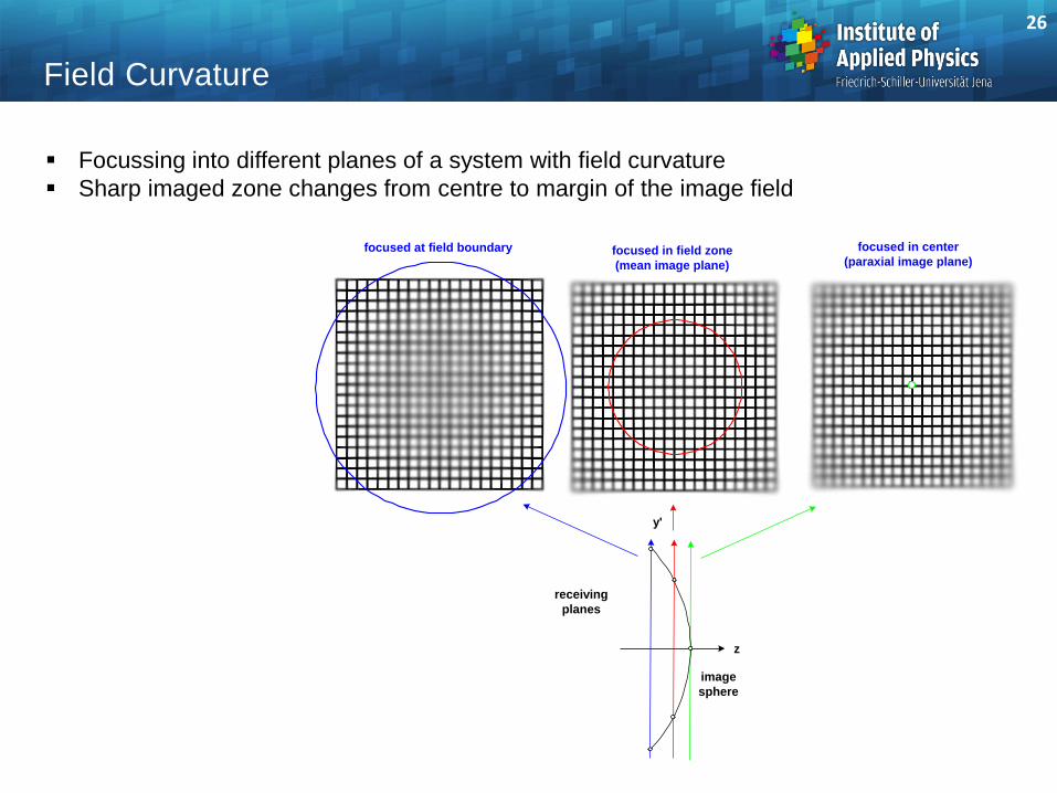
Focussing into different planes of a system with field curvature

Sharp imaged zone changes from centre to margin of the image field

focused in center

(paraxial image plane)focused in field zone

(mean image plane)

focused at field boundary

z

y'

receiving

planes

image

sphere

Field Curvature

26

Astigmatisms and Curvature of Field

DD D

ss s

best

sag'

' 'tan

2

D D D Ds s s spet sag pet' ' ' 'tan 3

D D Ds s sast sag' ' 'tan

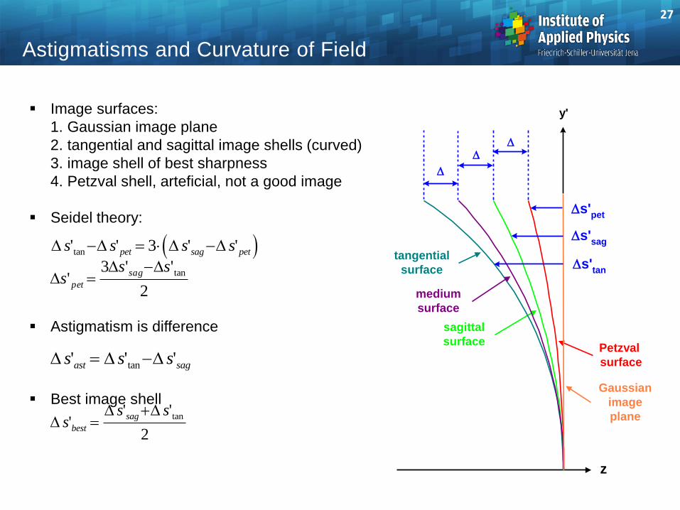
Image surfaces:

1. Gaussian image plane

2. tangential and sagittal image shells (curved)

3. image shell of best sharpness

4. Petzval shell, arteficial, not a good image

Seidel theory:

Astigmatism is difference

Best image shell

2

''3'

tansss

sag

pet

DDD

z

y'

Petzval

surface

sagittal

surface

tangential

surface

Gaussian

image

plane

medium

surface

Ds'sag

Ds'tan

Ds'pet

DD

D

27

28

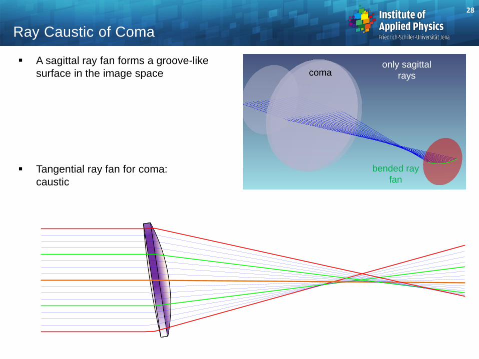
Ray Caustic of Coma

only sagittal

rays

bended ray

fan

coma

A sagittal ray fan forms a groove-like

surface in the image space

Tangential ray fan for coma:

caustic

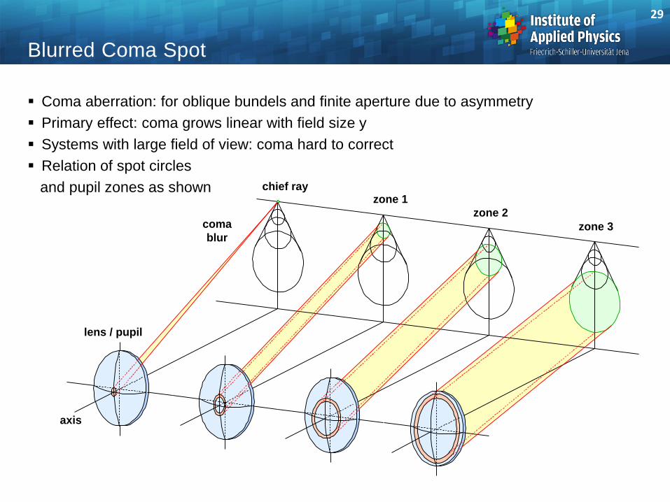
Blurred Coma Spot

Coma aberration: for oblique bundels and finite aperture due to asymmetry

Primary effect: coma grows linear with field size y

Systems with large field of view: coma hard to correct

Relation of spot circles

and pupil zones as shown

chief rayzone 1

zone 3

zone 2coma

blur

lens / pupil

axis

29

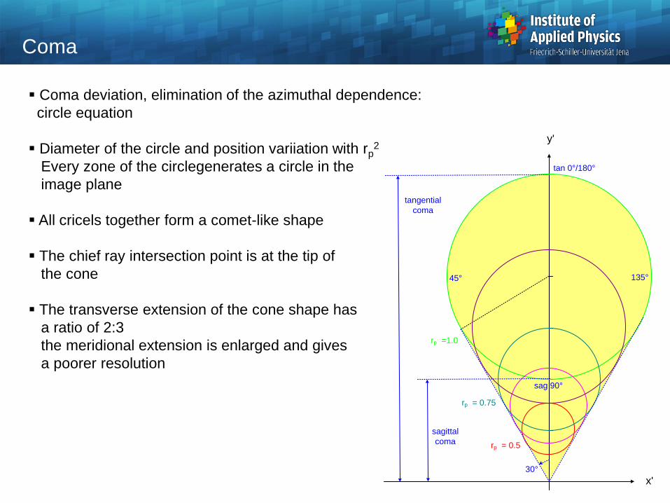
Coma

Coma deviation, elimination of the azimuthal dependence:

circle equation

Diameter of the circle and position variiation with rp2

Every zone of the circlegenerates a circle in the

image plane

All cricels together form a comet-like shape

The chief ray intersection point is at the tip of

the cone

The transverse extension of the cone shape has

a ratio of 2:3

the meridional extension is enlarged and gives

a poorer resolution

y'

30°

rp =1.0

sag 90°

tan 0°/180°

45° 135°

rp = 0.75

rp = 0.5

x'

sagittal

coma

tangential

coma

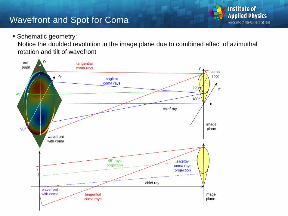
Wavefront and Spot for Coma

Schematic geometry:

Notice the doubled revolution in the image plane due to combined effect of azimuthal

rotation and tilt of wavefront

exit

pupiltangential

coma rays

sagittal

coma rays

image

plane

y'

x'

yp

xp

chief ray

coma

spot

90°

0°0°

180°

90°

45°

45° rays

projection

wavefront

with coma

tangential

coma rays

chief ray

wavefront

with coma image

plane

sagittal

coma rays

projection

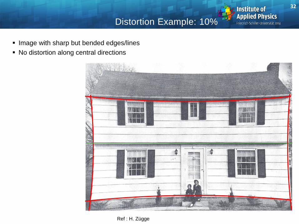
Distortion Example: 10%

Ref : H. Zügge

Image with sharp but bended edges/lines

No distortion along central directions

32

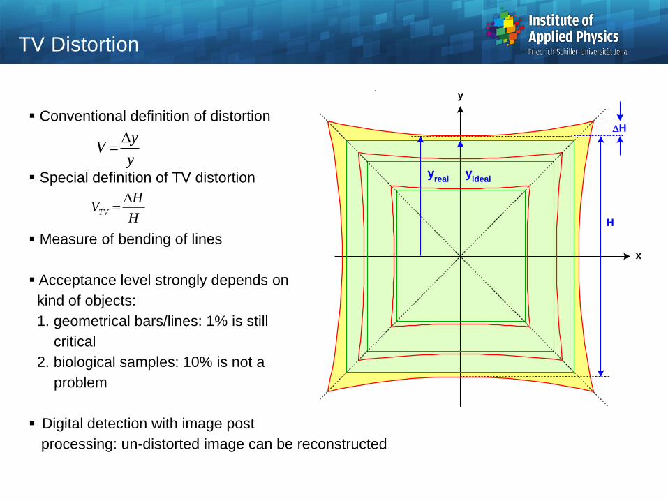
Conventional definition of distortion

Special definition of TV distortion

Measure of bending of lines

Acceptance level strongly depends on

kind of objects:

1. geometrical bars/lines: 1% is still

critical

2. biological samples: 10% is not a

problem

Digital detection with image post

processing: un-distorted image can be reconstructed

y

x

H

DH

yreal

yideal

y

yV

D

H

HVTV

D

TV Distortion

Purely geometrical deviations without any blurr

Distortion corresponds to spherical aberration of the chief ray

Important is the location of the stop:

defines the chief ray path

Two primary types with different sign:

1. barrel, D < 0

front stop

2. pincushion, D > 0

rear stop

Definition of local

magnification

changes

Distortion

pincussion

distortion

barrel

distortion

object

D < 0

D > 0

lens

rear

stop

imagex

x

y

y

y'

x'

y'

x'

front

stop

ideal

idealreal

y

yyD

'

''

34

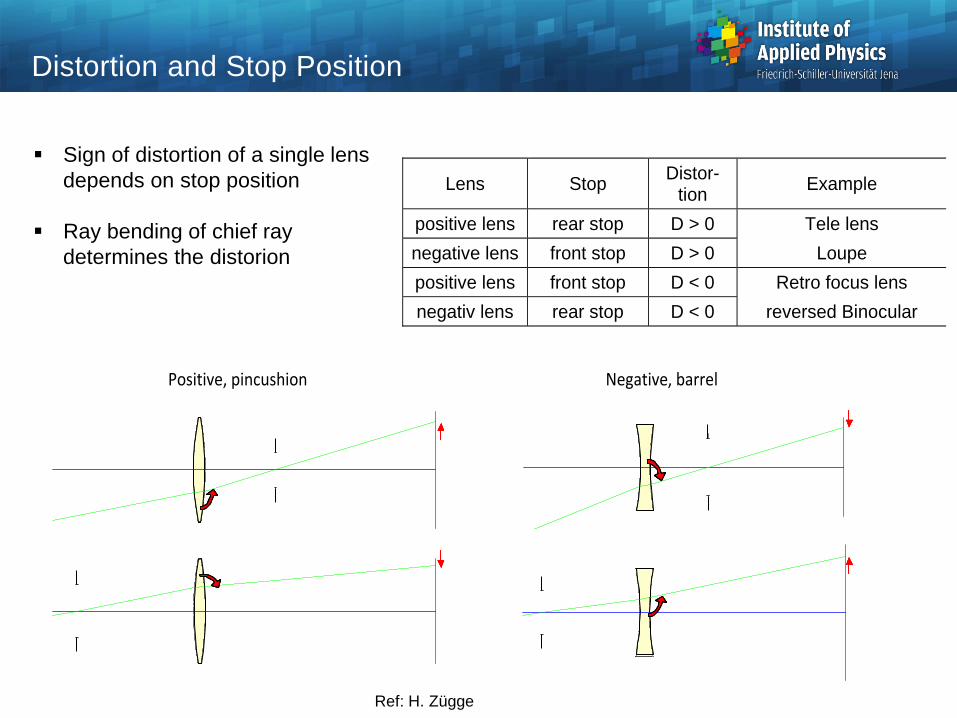
Distortion and Stop Position

Positive, pincushion Negative, barrel

Sign of distortion of a single lens

depends on stop position

Ray bending of chief ray

determines the distorion

Lens Stop Distor-

tion Example

positive lens rear stop D > 0 Tele lens

negative lens front stop D > 0 Loupe

positive lens front stop D < 0 Retro focus lens

negativ lens rear stop D < 0 reversed Binocular

Ref: H. Zügge

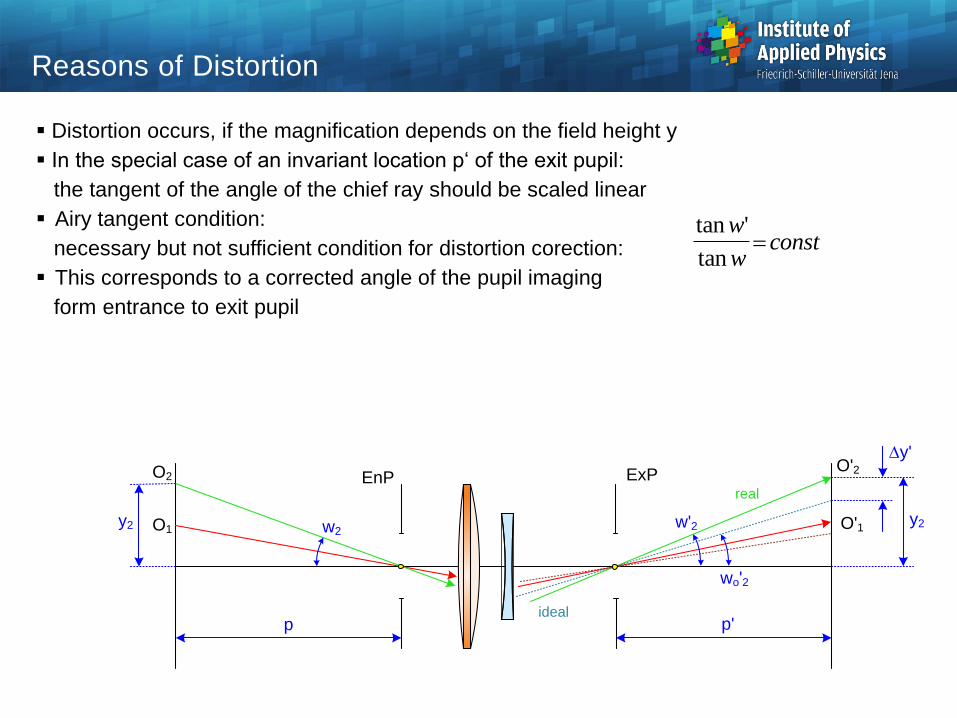
Distortion occurs, if the magnification depends on the field height y

In the special case of an invariant location p‘ of the exit pupil:

the tangent of the angle of the chief ray should be scaled linear

Airy tangent condition:

necessary but not sufficient condition for distortion corection:

This corresponds to a corrected angle of the pupil imaging

form entrance to exit pupil

Reasons of Distortion

O1

O2

O'1

O'2EnP ExP

w2w'2

ideal

real

y2 y2

p p'

Dy'

wo'2

tan '

tan

w

wconst

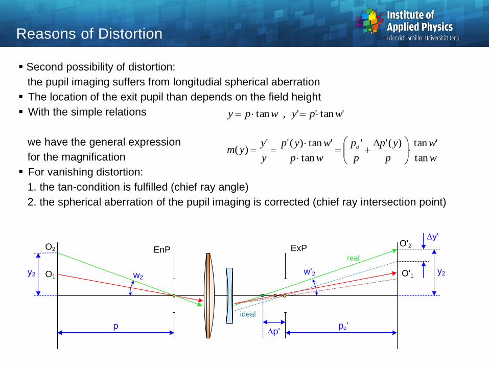
Second possibility of distortion:

the pupil imaging suffers from longitudial spherical aberration

The location of the exit pupil than depends on the field height

With the simple relations

we have the general expression

for the magnification

For vanishing distortion:

1. the tan-condition is fulfilled (chief ray angle)

2. the spherical aberration of the pupil imaging is corrected (chief ray intersection point)

Reasons of Distortion

O1

O2

O'1

O'2EnP ExP

w2w'2

ideal

real

y2 y2

p po'Dp'

Dy'

w

w

p

yp

p

p

wp

wyp

y

yym o

tan

'tan)(''

tan

'tan)('')(

D

'tan'',tan wpywpy

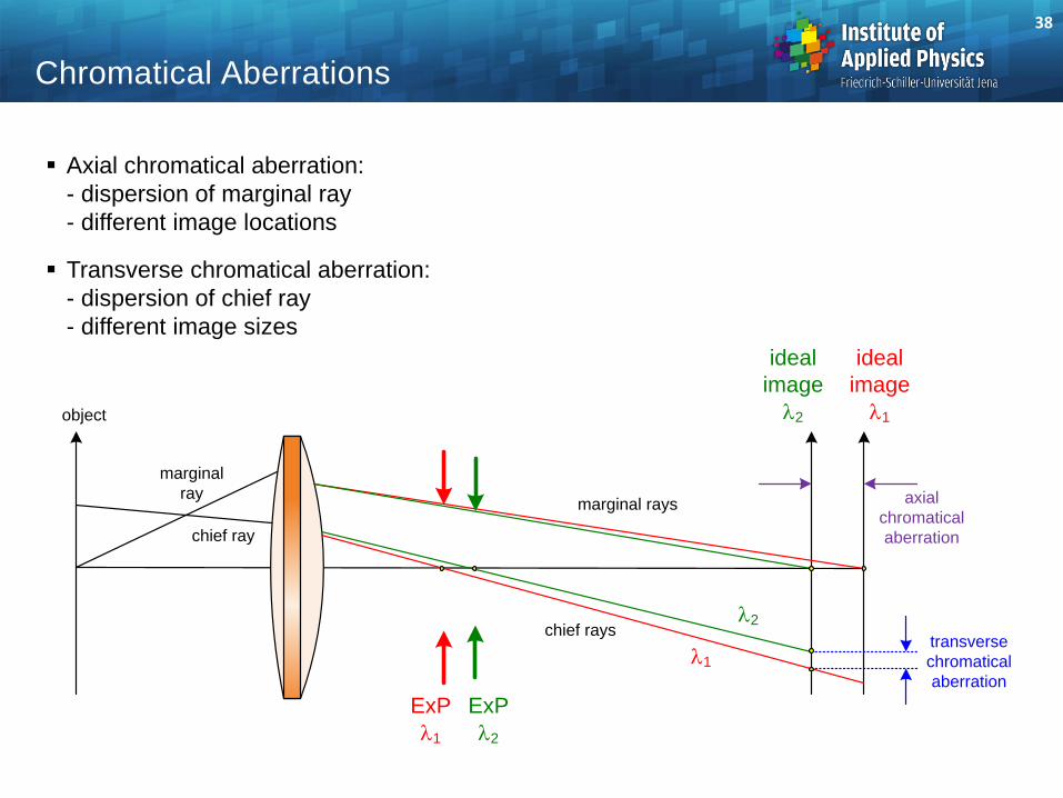
Axial chromatical aberration:

- dispersion of marginal ray

- different image locations

Transverse chromatical aberration:

- dispersion of chief ray

- different image sizes

38

Chromatical Aberrations

object

chief ray

marginal

ray

chief rays

marginal rays

l2

l1

ExP

l2

ExP

l1

transverse

chromatical

aberration

axial

chromatical

aberration

ideal

image

l1

ideal

image

l2

Axial Chromatical Aberration

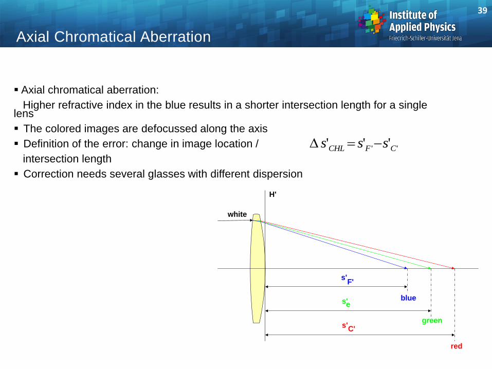
D s s sCHL F C' ' '' '

white

H'

s'F'

s'

s'

e

C'green

red

blue

Axial chromatical aberration:

Higher refractive index in the blue results in a shorter intersection length for a single lens

The colored images are defocussed along the axis

Definition of the error: change in image location /

intersection length

Correction needs several glasses with different dispersion

39

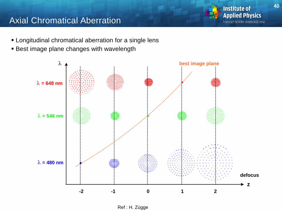
Axial Chromatical Aberration

z

l = 648 nm

defocus

-2 -1 0 1 2

l = 546 nm

l = 480 nm

best image planel

Longitudinal chromatical aberration for a single lens

Best image plane changes with wavelength

Ref : H. Zügge

40

sD

l

e C'F'

Axial Chromatical Aberration

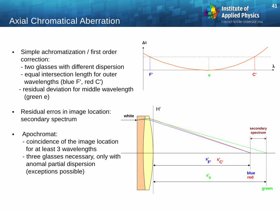
Simple achromatization / first order

correction:

- two glasses with different dispersion

- equal intersection length for outer

wavelengths (blue F', red C')

- residual deviation for middle wavelength

(green e)

Residual erros in image location:

secondary spectrum

Apochromat:

- coincidence of the image location

for at least 3 wavelengths

- three glasses necessary, only with

anomal partial dispersion

(exceptions possible)

white

H'

s'F'

s'

s'

e

C'

green

redblue

secondary

spectrum

41

stop

red

blue

reference

image

plane

y'CHV

D

'' ''' CFCHV yyy D

e

CFCHV

y

yyy

'

''' '' D

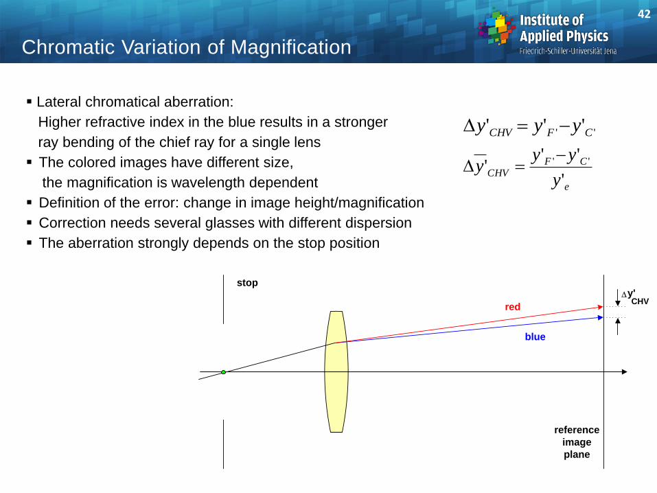
Chromatic Variation of Magnification

Lateral chromatical aberration:

Higher refractive index in the blue results in a stronger

ray bending of the chief ray for a single lens

The colored images have different size,

the magnification is wavelength dependent

Definition of the error: change in image height/magnification

Correction needs several glasses with different dispersion

The aberration strongly depends on the stop position

42

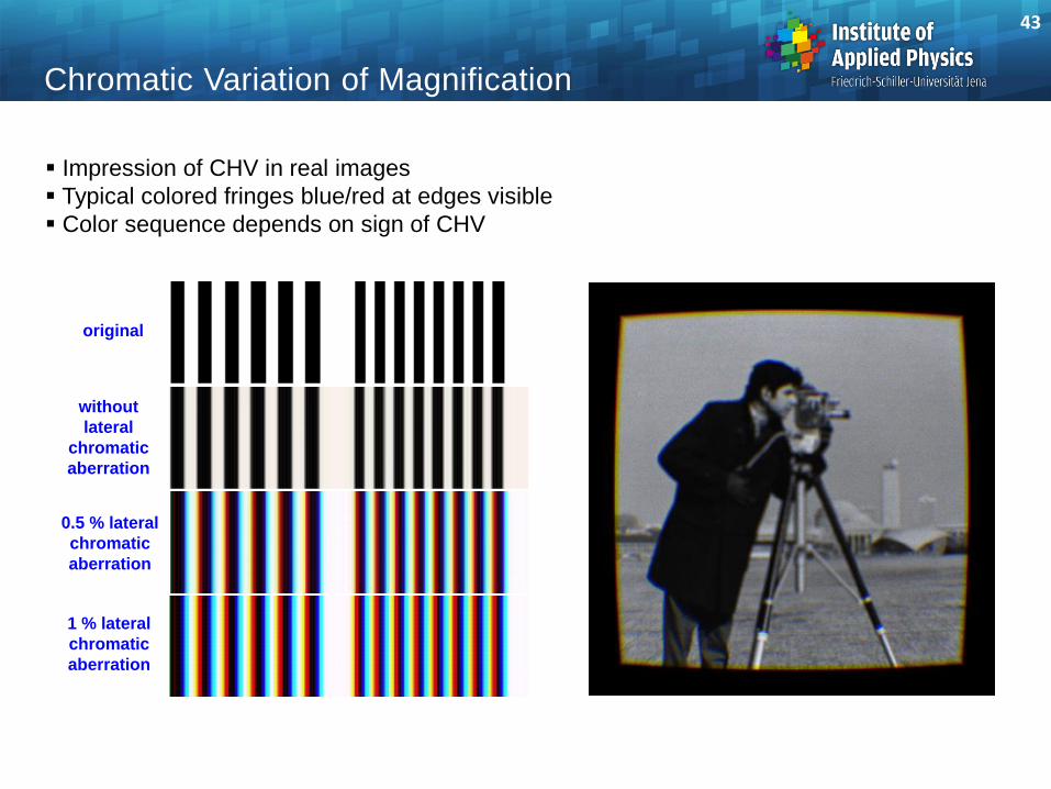
Impression of CHV in real images

Typical colored fringes blue/red at edges visible

Color sequence depends on sign of CHV

Chromatic Variation of Magnification

original

without

lateral

chromatic

aberration

0.5 % lateral

chromatic

aberration

1 % lateral

chromatic

aberration

43

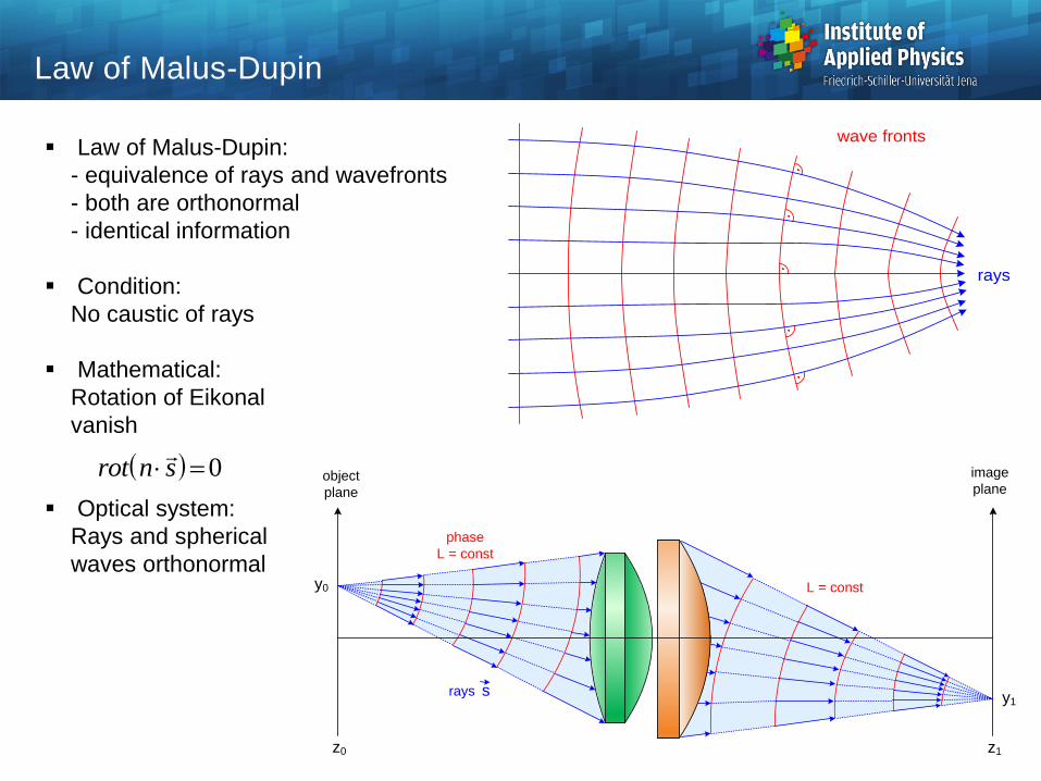
Law of Malus-Dupin:

- equivalence of rays and wavefronts

- both are orthonormal

- identical information

Condition:

No caustic of rays

Mathematical:

Rotation of Eikonal

vanish

Optical system:

Rays and spherical

waves orthonormal

wave fronts

rays

Law of Malus-Dupin

object

plane

image

plane

z0 z1

y1

y0

phase

L = const

L = const

srays

rot n s

0

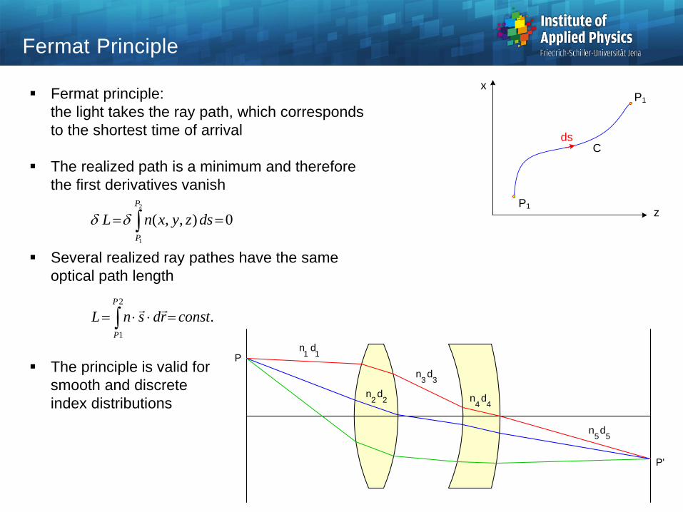
Fermat principle:

the light takes the ray path, which corresponds

to the shortest time of arrival

The realized path is a minimum and therefore

the first derivatives vanish

Several realized ray pathes have the same

optical path length

The principle is valid for

smooth and discrete

index distributions

Fermat Principle

P1

x

z

P1

Cds

2

1

0),,(

P

P

dszyxnL

2

1

.

P

P

constrdsnL

P'

Pn d1 1

n d2 2

n d3 3

n d4 4

n d5 5

Wave Aberration in Optical Systems

Definition of optical path length in an optical system:

Reference sphere around the ideal object point through the center of the pupil

Chief ray serves as reference

Difference of OPL : optical path difference OPD

Practical calculation: discrete sampling of the pupil area,

real wave surface represented as matrix

Exit plane

ExP

Image plane

Ip

Entrance pupil

EnP

Object plane

Op

chief

ray

w'

reference

sphere

wave

front

W

y yp y'p y'

z

chief

ray

wave

aberration

optical

systemupper

coma ray

lower coma

ray

image

point

object

point

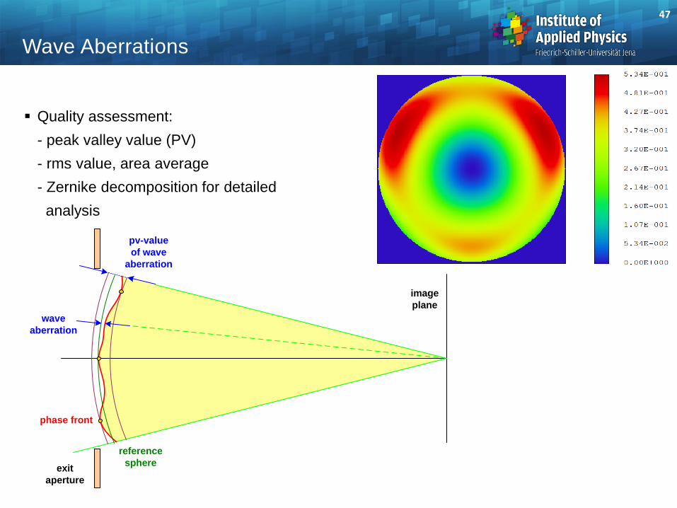
47

Wave Aberrations

Quality assessment:

- peak valley value (PV)

- rms value, area average

- Zernike decomposition for detailed

analysis

exit

aperture

phase front

reference

sphere

wave

aberration

pv-value

of wave

aberration

image

plane

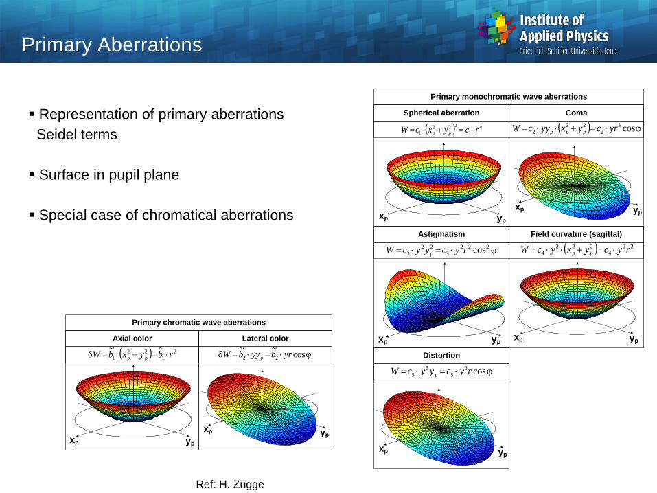
Representation of primary aberrations

Seidel terms

Surface in pupil plane

Special case of chromatical aberrations

Primary Aberrations

Spherical aberration Coma

Primary monochromatic wave aberrations

Astigmatism Field curvature (sagittal)

Distortion

ypxp

ypxp

ypxp

ypxp

ypxp

4

1

222

1 rcyxcW pp cos3

2

22

2 yrcyxyycW ppp

222

3

22

3 cosrycyycW p 22

4

222

4 rycyxycW pp

cos3

5

3

5 rycyycW p

Axial color Lateral color

Primary chromatic wave aberrations

2

1

22

1

~~rbyxbW pp

ypxp

ypxp

cos~~

22 yrbyybW p

Ref: H. Zügge

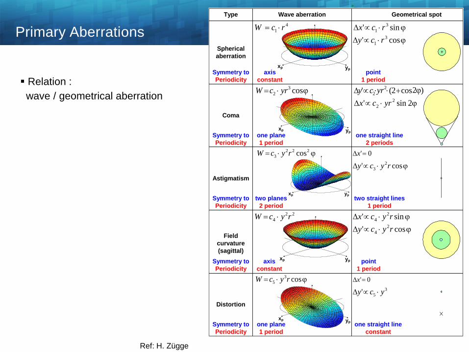
Relation :

wave / geometrical aberration

Primary Aberrations

Type

ypxp

ypxp

ypxp

ypxp

ypxp

4

1 rcW

cos3

2 yrcW

222

3 cosrycW

22

4 rycW

cos3

5 rycW

D sin' 3

1 rcx

D cos' 3

1 rcy

D 2sin' 2

2 yrcx

0'Dx

D cos' 2

3 rycy

D sin' 2

4 rycx

D cos' 2

4 rycy

0'Dx

3

5' ycy D

Spherical

aberration

Symmetry to

Periodicity

axis

constant

point

1 period

Wave aberration Geometrical spot

Coma

Astigmatism

Field

curvature

(sagittal)

Distortion

Symmetry to

Periodicity

Symmetry to

Periodicity

Symmetry to

Periodicity

Symmetry to

Periodicity

one plane

1 period

two planes

2 period

one plane

1 period

axis

constant

point

1 period

one straight line

constant

one straight line

2 periods

two straight lines

1 period

)2cos2('2

2D yrcy

Ref: H. Zügge

01

0cos

0sin

)(),(

mfür

mfürm

mfürm

rRrZ m

n

m

n

''

0'*

'

1

0

2

0)1(2

1),(),( mmnn

mm

n

m

nn

drrdrZrZ

n

n

nm

m

nnm rZcrW ),(),(

1

0

*

2

00

),(),(1

)1(2drrdrZrW

nc m

n

m

nm

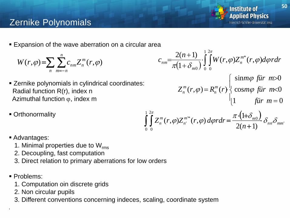
Zernike Polynomials

Expansion of the wave aberration on a circular area

Zernike polynomials in cylindrical coordinates:

Radial function R(r), index n

Azimuthal function , index m

Orthonormality

Advantages:

1. Minimal properties due to Wrms

2. Decoupling, fast computation

3. Direct relation to primary aberrations for low orders

Problems:

1. Computation oin discrete grids

2. Non circular pupils

3. Different conventions concerning indeces, scaling, coordinate system ,

50

Zernike Polynomials

+ 6

+ 7

- 8

m = + 8

0 5 8764321n =

cos

sin

+ 5

+ 4

+ 3

+ 2

+ 1

0

- 1

- 2

- 3

- 4

- 5

- 6

- 7

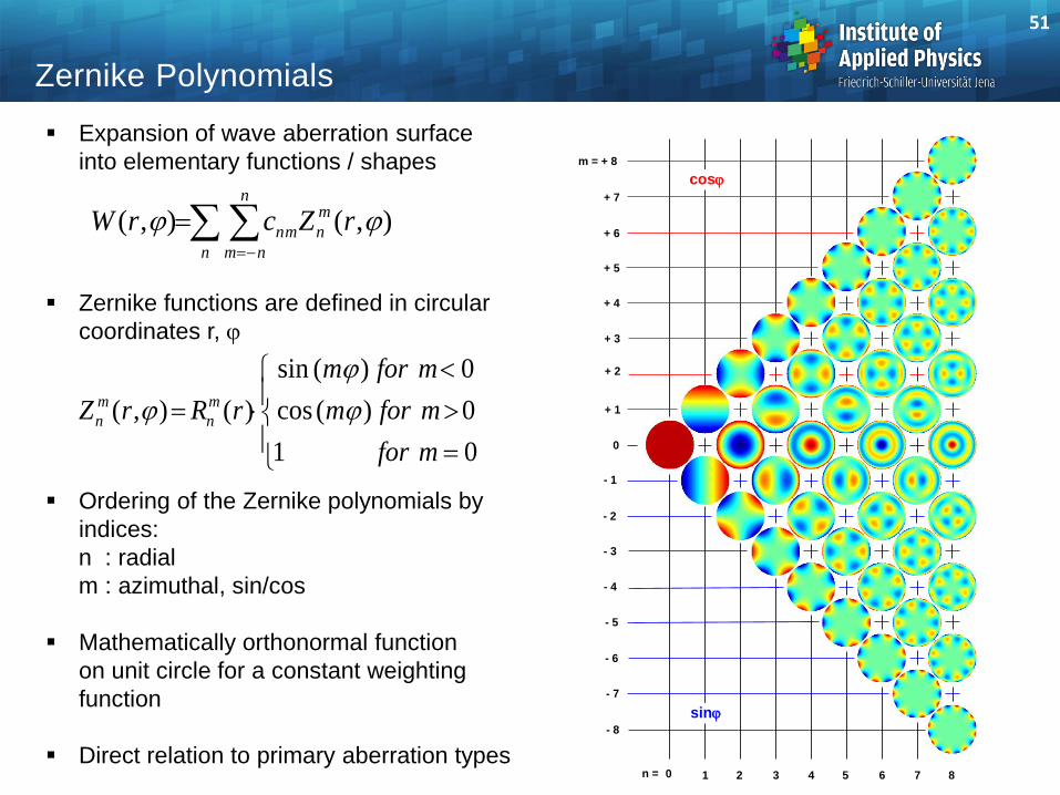
Expansion of wave aberration surface into elementary functions / shapes

Zernike functions are defined in circular coordinates r,

Ordering of the Zernike polynomials by indices:

n : radial

m : azimuthal, sin/cos

Mathematically orthonormal function on unit circle for a constant weighting function

Direct relation to primary aberration types

n

n

nm

m

nnm rZcrW ),(),(

01

0)(cos

0)(sin

)(),(

mfor

mform

mform

rRrZ m

n

m

n

51

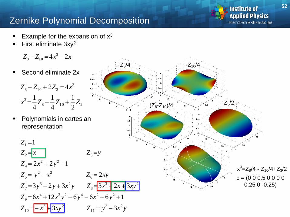
Zernike Polynomial Decomposition

Example for the expansion of x3

First eliminate 3xy2

Second eliminate 2x

Polynomials in cartesian representation

52

Z8/4 -Z10/4

(Z8-Z10)/4Z3/2

x3=Z8/4 - Z10/4+Z3/2

c = (0 0 0.5 0 0 0 0

0.25 0 -0.25)

yxyZxyxZ

yxyyxxZ

xyxxZyxyyZ

xyZxyZ

yxZ

yZxZ

Z

23

11

23

10

224224

9

23

8

23

7

6

22

5

22

4

32

1

33

1666126

323323

2

122

1

xxZZ 24 3

108

2108

3

3

2108

2

1

4

1

4

1

42

ZZZx

xZZZ

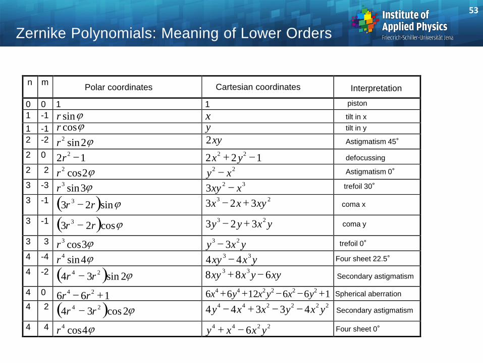
Zernike Polynomials: Meaning of Lower Orders

n m Polar coordinates

Interpretation

0 0 1 1 piston

1 -1 r sin x

Four sheet 22.5°

1 - 1 r cos y

2 -2 r 2

2 sin 2 xy

2 0 2 1 2

r 2 2 1 2 2

x y

2 2 r 2

2 cos y x 2 2

3 -3 r 3

3 sin 3 2 3

xy x

3 -1 3 2 3

r r sin 3 2 3 3 2

x x xy

3 - 1 3 2 3

r r cos 3 2 3 3 2

y y x y

3 3 r 3

3 cos y x y 3 2

3

4 -4 r 4

4 sin 4 4 3 3

xy x y

4 -2 4 3 2 4 2

r r sin 8 8 6 3 3

xy x y xy

4 0 6 6 1 4 2

r r 6 6 12 6 6 1 4 4 2 2 2 2 x y x y x y

4 2 4 3 2 4 2

r r cos 4 4 3 3 4 4 4 2 2 2 2

y x x y x y

4 4 r 4

4 cos y x x y 4 4 2 2

6

Cartesian coordinates

tilt in y

tilt in x

Astigmatism 45°

defocussing

Astigmatism 0°

trefoil 30°

trefoil 0°

coma x

coma y

Secondary astigmatism

Secondary astigmatism

Spherical aberration

Four sheet 0°

53

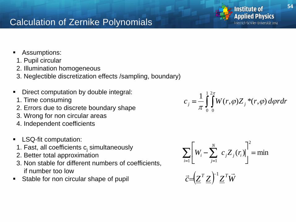
drrdrZrWc jj

),(*),(1

1

0

2

0

min)(

2

1 1

i

ijj

N

j

i rZcW

WZZZcTT 1

Calculation of Zernike Polynomials

Assumptions:

1. Pupil circular

2. Illumination homogeneous

3. Neglectible discretization effects /sampling, boundary)

Direct computation by double integral:

1. Time consuming

2. Errors due to discrete boundary shape

3. Wrong for non circular areas

4. Independent coefficients

LSQ-fit computation:

1. Fast, all coefficients cj simultaneously

2. Better total approximation

3. Non stable for different numbers of coefficients,

if number too low

Stable for non circular shape of pupil

54