memorandum - ross mckitrick - ross mckitrick … · 2010-07-13 · temperatures after 1990 cannot...
TRANSCRIPT

Memorandum From: Ross McKitrick, Ph.D. Professor of Economics University of Guelph [email protected] To: Air and Radiation Docket and Information Center, Environmental Protection Agency, Mailcode: 2822T, 1200 Pennsylvania Ave., NW., Washington, DC 20460. [email protected] Joe Dougherty, Office of Air and Radiation, E-mail address: [email protected] Date: November 24, 2008 Re: Advanced Notice of Proposed Rulemaking(ANPR) for Greenhouse Gases Under the
Clean Air Act, EPA-HQ-OAR-2008-0318-0117
The following comments are related to the issues raised in the ANPR and in the Endangerment Technical Support Document
I. Would it be appropriate to use the most recent IPCC report and the U.S. government Climate
Change Science Program synthesis reports as scientific assessments that could serve as an
important source or as the primary basis for the EPA’s issuance of “air quality criteria” ?
The most recent IPCC Report (the Fourth Assessment Report or AR4) drew considerable attention to the global mean surface temperature records, and comparatively less to the global mean tropospheric temperature records. For example, the Summary for Policymakers Figure SPM.3 prominently displays a global average surface temperature, but provides no such figure for the lower or mid-troposphere. This is indicative of bias for three reasons: 1. All the climate models used by the IPCC for diagnosing the causes of historical warming and
predictions of future warming indicate that the predominant characteristic of greenhouse gas-induced warming will be a differentially strong warming of the troposphere over the tropics (see, e.g., IPCC Figure 9.1). Yet nearly 30 years of satellite data are available and they do not support this prediction. The text of the IPCC and the Climate Change Science Program Reports concede this discrepancy (see Appendix B below) and its potential significance as evidence that the climate system is not as
College of Management and Economics
DEPARTMENT OF ECONOMICS

EPA: Advance Notice of Proposed Rulemaking Submission November 24, 2008 Submission by Ross McKitrick
2
sensitive to greenhouse gases as models typically indicate. The failure to show the tropospheric temperature data in the Summary for Policymakers, and the failure to graph the tropospheric data in the body of the report in a form comparable to the model predictions, amounts to concealment of material counterevidence to the conclusions they were emphasizing in the Summary.
2. There is a substantial body of peer-reviewed evidence that the surface temperature records are
deficient for the purpose of measuring long-term climate change. Global surface temperature averages are produced from subsamples of the archive of the Global Historical Climatology Network maintained by the National Climatic Data Center at NOAA. Yet the GHCN stopped updating records from thousands of locations around the world in the early 1990s, either because the weather records in the host country ceased or GHCN simply dropped the record. The number of available temperature samples fell from about 12,000 per year to about 8,000 per year between 1990 and 1992, coinciding with the jump in the raw temperature average from about 10 oC to about 11 oC.
Groups who produce the global average temperature series relied upon by the IPCC, such as the
Climate Research Unit in the UK and the Goddard Institute of Space Studies at NASA must attempt to adjust for this discontinuity. But the underlying problem means that reports of elevated mean temperatures after 1990 cannot be assumed to be climatic in origin, as they may instead reflect a failure to correct the bias induced by the collapsed sample. This kind of sampling discontinuity would be unacceptable in official statistics such as the Consumer Price Index or the Gross National Product. Since there is no such discontinuity in the satellite records, and since they measure the layers of the atmosphere of most direct interest for monitoring the effects of greenhouse gases, they should be the primary source for presenting information about global atmospheric warming. Yet the IPCC Summary makes no mention of the sampling problems nor does it present the satellite data. These material omissions are indicative of bias.

EPA: Advance Notice of Proposed Rulemaking Submission November 24, 2008 Submission by Ross McKitrick
3
3. Early drafts of the IPCC Report ignored the peer-reviewed literature showing that the spatial pattern of surface temperature trends over land after 1980 is highly correlated with the spatial pattern of socioeconomic activity and industrialization, and that these non-climatic influences add a large upward bias to the post-1980 surface temperature data. After repeated demands by reviewers to address the topic, the final text of the IPCC Report (Chapter 3 page 244) contained the following paragraph (emphasis added), which was inserted after the close of scientific review:
McKitrick and Michaels (2004) and De Laat and Maurellis (2006) attempted to demonstrate that geographical patterns of warming trends over land are strongly correlated with geographical patterns of industrial and socioeconomic development, implying that urbanisation and related land surface changes have caused much of the observed warming. However, the locations of greatest socioeconomic development are also those that have been most warmed by atmospheric circulation changes (Sections 3.2.2.7 and 3.6.4), which exhibit
large-scale coherence. Hence, the correlation of warming with industrial and
socioeconomic development ceases to be statistically significant. In addition, observed warming has been, and transient greenhouse-induced warming is expected to be, greater over land than over the oceans (Chapter 10), owing to the smaller thermal capacity of the land.
The IPCC asserts that the significant correlation between temperature change and industrialization is
an artifact of natural atmospheric oscillations. However, the cited sections of the report (3.2.2.7 and 3.6.4) provide no evidence for such a claim. Moreover, the highlighted phrase claims that once this effect is accounted for, the correlations become statistically insignificant. “Statistical insignificance” is a specific scientific assertion, yet no empirical evidence for this statement is provided anywhere in the IPCC Report, nor do they cite any peer reviewed publication to support it. It is a fabrication. It is, moreover, false, as I have shown in a working paper1 in which I augment a surface temperature model with indicators of major atmospheric circulation systems and test for their influence. After controlling for their effects the correlations between surface temperature changes and socioeconomic development remain as significant as before.
The IPCC was therefore in possession of peer-reviewed scientific evidence showing that the key data
set on which they based their most prominent scientific conclusions was contaminated with a significant warming bias, but rather than report this fact the Lead Authors fabricated evidence to justify ignoring the problem. This fact alone should render the IPCC Fourth Assessment Report invalid as a basis for policymaking.
The Climate Change Science Report (CCSP) of 2006 suffers from a failure to subject models to appropriate skepticism, and where observational data contradict model outputs, the CCSP denigrates the data rather than considering whether the models might be in error. In Its Executive Summary the CCSP report describes a “potentially serious inconsistency” (p. 11) between model predictions and observed data in the tropical troposphere. All models predict amplified warming in the tropical troposphere as an essential component of the assumed greenhouse gas-induced global warming mechanism. Yet the numerous data sets analysed and scrutinized in the CCSP report fail to show this pattern. Rather than acknowledge that the models appear to be wrong, the CCSP report claims that
1 McKitrick, Ross (2008) “Atmospheric Oscillations do not Explain the Temperature-Industrialization Correlation” (July 21, 2008). Available at SSRN: http://ssrn.com/abstract=1166424. Under review.
EPA: Advance Notice of Proposed Rulemaking Submission November 24, 2008 Submission by Ross McKitrick
4
the models are probably right and the data are probably wrong, despite their failure across six chapters to find any specific flaws in the data beyond the ones that were rectified as part of the report-writing process:
This difference between models and observations may arise from errors that are common to all models, from errors in the observational data sets, or from a combination of these factors. The second explanation is favored, but the issue is still open. (CCSP Report page 2)
Later (pages 10-11) the Summary cites model-to-model comparisons as evidence that the models are likely correct, and repeats its claim that the data are likely wrong. They go on to explain that to get agreement between models and data requires an assumption that greenhouse gases have little climatic impact, but then dismiss the assumption as unrealistic:
Figure 4G shows that the lower troposphere warms more rapidly than the surface in almost all model simulations, while, in the majority of observed data sets, the surface has warmed more rapidly than the lower troposphere. In fact, the nature of this discrepancy is not fully captured in Fig. 4G as the models that show best agreement with the observations are those that have the lowest (and probably unrealistic) amounts of warming.
Thus the CCSP decides on a model’s “realism” not by its ability to match the data, but by how much its behaviour matches the modelers’ assumptions. The controlling influence of this assumption is evident throughout the CCSP report and, in my view, substantially diminishes the credibility of its conclusions.
2. What is the adequacy of the available scientific literature [synthesis reports such as the
Intergovernmental Panel on Climate Change’s Fourth Assessment Report and various reports of
the US Climate Change Science Program] ?
It is a mistake to equate the “scientific literature” with the IPCC and CCSP reports. These reports draw from the scientific literature to argue for specific conclusions. They should be viewed as briefs for one side. Taken as a whole the scientific literature contains important information downplayed or excluded from the IPCC and CCSP reports which undermines their conclusions. For instance, hydroclimatic data exhibit inertial patterns called long term persistence (Koutsoyiannis and Montanari 2007, Cohn and Lins 2005) or, in nonstationarity frameworks, persistency (Kärner 2002). Failure to control for such patterns can lead to false trend detection, by overstating the statistical significance of a trend. Cohn and Lins (2005) showed that what appears to be a significant trend in the 20th century mean Northern Hemisphere temperature data falls to only marginal significance when using a persistence-robust test. The Second-Order Draft of the IPCC Report (page 3-9) contained the following discussion of this issue:
Determining the statistical significance of a trend line in geophysical data is difficult, and many oversimplified techniques will tend to overstate the significance. Zheng and Basher (1999), Cohn and Lins (2005) and others have used time series methods to show that failure

EPA: Advance Notice of Proposed Rulemaking Submission November 24, 2008 Submission by Ross McKitrick
5
to properly treat the pervasive forms of long-term persistence and autocorrelation in trend residuals can make erroneous detection of trends a typical outcome in climatic data analysis.
A similar comment appeared in the draft chapter appendix, though it included a disputatious and unsupported assertion that LTP models lack physical realism, to which I presented a counterargument in my second draft review comments. The above paragraph has direct bearing on the overall conclusions of the IPCC report. But without explanation, and against reviewer instructions, it was deleted from the published edition. The entry in the Appendix was made even more disputatious, even though no supporting citations were provided for their dismissal of Cohn and Lins’ results. These changes were not subject to peer review. Another example concerns paleoclimatic evidence. IPCC (1990) presented evidence of a Medieval Warm Period spanning ~900 to 1300 AD, during which the climate was perhaps warmer than the late 20th century. In IPCC (2001), a new conclusion based on Mann et al. (1998, 1999) was the ‘hockey stick graph,’ which showed no Medieval Warm Period and a recent warming unprecedented in the past thousand years. Subsequent analysis (e.g. Bürger and Cubasch 2005, McIntyre and McKitrick 2003, 2005a, 2005b; Wegman et al. 2006, NRC 2006) showed that Mann’s methodology understated historical uncertainty, and relied for its conclusions on controversial ‘bristlecone pine’ data with a steep 20th-century trend unrelated to temperature. IPCC (2007) changed to a suite of paleoclimate reconstructions demonstrating greater uncertainty about past trends. Wegman et al. (2006) note that many of these reconstructions reuse Mann’s bristlecones. The NRC (2006) and Wegman et al. (2006) reports undermine the conclusion that the 1990s were unusually warm. The final, published text of the IPCC report ignored the findings of the NRC and Wegman panel reports, thoroughly misrepresented the hockey stick debate, and relied on unpublished claims by Wahl and Ammann despite reviewer demands that reference to these papers be removed since they failed to meet the IPCC publication deadlines (see Holland 2007). The question of whether greenhouse gases affect the climate is also handled from a one-sided perspective in the IPCC Report. Climate models (General Circulation Models or GCMs) make several specific predictions of what should already be observed if increased greenhouse gases are the dominant climate forcing. (i) Warming in the tropical region (half the planet’s surface) should strengthen with altitude, and maximum planetary warming should be in the troposphere over the tropics (IPCC 2007 Figs. 9.1 and 10.7, CCSP 2006 Figs. 1.3 and 5.7). (ii) Arctic surface warming should weaken with altitude (sources as in (i)). (iii) Global mean wind speeds should be decreasing by 0.8% per decade (Wentz et al. 2007). (iv) No correlation should exist between the spatial pattern of warming over land and the spatial pattern of industrialization (discussed above). (v) Global temperature averages should exhibit persistency (Kärner 2002).

EPA: Advance Notice of Proposed Rulemaking Submission November 24, 2008 Submission by Ross McKitrick
6
Observed data contradict all these predictions. (i) Satellite and balloon data show little warming in the tropical troposphere--see Figure 1 and IPCC (2007) Fig. 3.4, CCSP (2006) Fig. 5.4, Douglass et al. (2007), Chase et al. (2004). Any observed warming occurs at rates below the global surface average. Allen and Sherwood (2008) proposed that a tropospheric temperature field inferred from the wind field might match GCMs better, but none of the satellite or thermometer-based balloon series support this result. (ii) Observed Arctic warming strengthens with altitude in a pattern consistent with predominantly natural forcing, but inconsistent with greenhouse forcing (Graversen et al. 2008). (iii) Global mean wind speeds have increased by about 1% per decade since 1987 (Wentz et al. 2007) (iv) The spatial pattern of warming over land is strongly correlated with that of industrialization (de Laat and Maurellis 2004, 2006; McKitrick and Michaels 2004, 2007). (v) Atmospheric temperature data exhibit antipersistency (Kärner 2002, 2005) consistent with predominant solar forcing but inconsistent with predominant greenhouse forcing (Kärner 2002). The IPCC cites attribution studies (Stott et al. 1999 etc) that examine only a few explanations for modern climate trends: greenhouse gases, aerosol pollution, total solar irradiance, stratospheric ozone depletion and volcanic eruptions. Explanations unrepresented in the standard GCM framework include:
• Surface data contamination from non-climatic effects (discussed above) and land-use change more generally (Pielke Sr. et al., 2002, 2007, Christy et al. 2006, Feddema et al. 2005)
• Chaotic processes governing interactions of major oscillatory components of the climate system over time (Essex et al. 1987, Tsonis et al. 2007)
• Effects of galactic cosmic rays and the sun’s fluctuating magnetic shield on low cloud cover (Marsh and Svensmark 2004, Shaviv and Veizer 2003, Scherer et al 2006)
• Negative feedback between tropical cloud formation and regional temperature changes (Lindzen et al. 2000, Spencer and Braswell 2008)
Published evidence shows each of these factors likely have significant climatic effects. None has been ruled out by the studies relied on by the IPCC. Hence it is not possible to conclude that surface warming must be attributable to greenhouse gases, and the strongly-worded conclusions of the IPCC are not justified by the actual state of the science.
Popular views are heavily influenced by the IPCC, but it has critics as well as supporters. Bray and von Storch (2006) present survey evidence questioning whether the IPCC enjoys majority support among professional climate scientists. Holland (2007) and McKitrick (2008) review cases in which IPCC (2007) excluded or selectively reported published evidence against global warming. Henderson (2007) reviews evidence of bias, including political advocacy by the IPCC’s governing bureau. Taken together these things indicate that the IPCC Reports should not be considered adequate as a basis for large, expensive policy decisions.
Yours truly,

EPA: Advance Notice of Proposed Rulemaking Submission November 24, 2008 Submission by Ross McKitrick
7
Ross McKitrick Professor
Appendix A: Response to Hon. J. Dingell, November 4, 2008
Appendix B: Response to Sen. J. Inhofe, November 18, 2008
References
Bray, Dennis and Hans von Storch (2007) “The Perspectives of Climate Scientists on Global Climate Change.” Institute for Coastal Research Research Report 2007-11, Geestacht. http://dvsun3.gkss.de/BERICHTE/GKSS_Berichte_2007/GKSS_2007_11.pdf
Bürger, Gerd, and Ulrich Cubasch. 2005. Are multiproxy climate reconstructions robust? Geophysical Research Letters 32 (December 14): L23711. doi:10.1029/2005GL024155.
CCSP (Climate Change Science Program). 2006. Temperature Trends in the Lower Atmosphere: Steps for Understanding and Reconciling Differences. Thomas R. Karl, Susan J. Hassol, Christopher D. Miller, and William L. Murray, editors, 2006. A Report by the Climate Change Science Program and the Subcommittee on Global Change Research, Washington, DC.
Chase, T. N., R. A. Pielke Sr, B. Herman, and X. Zeng. 2004. Likelihood of rapidly increasing surface temperatures unaccompanied by strong warming in the free troposphere. Climate Research 25, no. 3: 185-190.
Christy, John R., William B. Norris, Kelly Redmond, and Kevin P. Gallo. 2006. Methodology and Results of Calculating Central California Surface Temperature Trends: Evidence of Human-Induced Climate Change? Journal of Climate 19, no. 4 (February 1): 548-563 .
Cohn, Timothy A. , and Harry F. Lins. 2005. Nature's style: Naturally trendy. Geophysical Research Letters 32 (December 1): 23402.
de Laat, A. T. J. , and A. N. Maurellis. 2004. Industrial CO2 emissions as a proxy for anthropogenic influence on lower tropospheric temperature trends. Geophysical Research Letters 31 (March 1): 05204.
de Laat, A. T. J. , and A. N. Maurellis. 2006. Evidence for influence of anthropogenic surface processes on lower tropospheric and surface temperature trends. International Journal of Climatology 26 (June 1): 897-913.
Douglass, D. H., J. R. Christy, B. D. Pearson, and S. F. Singer. 2007. A comparison of tropical temperature trends with model predictions. Intl J Climatology (Royal Meteorol Soc). DOI 10.
Essex, Christopher, Turab Lookman, and M. A. H. Nerenberg. 1987. The climate attractor over short timescales. Nature 326, no. 6108 (March 5): 64-66. doi:10.1038/326064a0.
Feddema, Johannes J., Keith W. Oleson, Gordon B. Bonan, et al. 2005. The Importance of Land-Cover Change in Simulating Future Climates. Science 310, no. 5754 (December 9): 1674-1678. doi:10.1126/science.1118160.
Graversen, R. G., T. Mauritsen, M. Tjernstrom, E. Kallen, and G. Svensson. 2008. Vertical structure of recent Arctic warming. Nature 451, no. 7174: 53-6.
Holland, David (2007) “Bias and Concealement in the IPCC Process: The “Hockey Stick” Affair and Its Implications.” Energy and Environment Volume 18, Numbers 7-8, December 2007 , pp. 951-983(33).
Intergovernmental Panel on Climate Change (IPCC) Working Group I (1990) Climate Change: The IPCC Scientific Assessment. Cambridge: Cambridge University Press.

EPA: Advance Notice of Proposed Rulemaking Submission November 24, 2008 Submission by Ross McKitrick
8
Intergovernmental Panel on Climate Change. (2001), Climate Change 2001: The Scientific Basis. Houghton, J.T., Y. Ding, D.J. Griggs, M. Noguer, P.J. van der Linden, X. Dai, K. Maskell and C.A. Johnson CA., eds. Cambridge: Cambridge University Press.
IPCC, 2007: Climate Change 2007: The Physical Science Basis. Contribution of Working Group I to the Fourth Assessment Report of the Intergovernmental Panel on Climate Change Solomon, S., D. Qin, M. Manning, Z. Chen, M. Marquis, K.B. Averyt, M. Tignor and H.L. Miller (eds.). Cambridge University Press, Cambridge, United Kingdom and New York, NY, USA, 996 pp.
Kärner, O. 2002. On nonstationarity and antipersistency in global temperature series. Journal of Geophysical Research 107, no. D20 (October 18): 4415. doi:10.1029/2001JD002024.
Kärner, Olavi. 2005. Some examples of negative feedback in the Earth climate system. Central European Journal of Physics 3 (June 1): 190-208.
Koutsoyiannis, Demetris, and Alberto Montanari. 2007. Statistical analysis of hydroclimatic time series: Uncertainty and insights. Water Resources Research 43 (May 22): W05429. doi:10.1029/2006WR005592.
Mann, Michael E. , Raymond S. Bradley, and Malcolm K. Hughes. 1999. Northern hemisphere temperatures during the past millennium: Inferences, uncertainties, and limitations. Geophysical Research Letters 26 (March 1): 759-762.
Mann, Michael E., Raymond S. Bradley, and Malcolm K. Hughes. 1998. Global-scale temperature patterns and climate forcing over the past six centuries. Nature 392, no. 6678 (April 23): 779-787. doi:10.1038/33859.
Marsh, Nigel, and Henrik Svensmark. 2000. Cosmic Rays, Clouds, and Climate. Space Science Reviews 94, no. 1 (November 1): 215-230. doi:10.1023/A:1026723423896.
McIntyre, S. and R. McKitrick (2005b), “The M&M Critique of the MBH98 Northern Hemisphere Climate Index: Update and Implications.” Energy and Environment, 16, 69-99.
McIntyre, S. and R. McKitrick, 2003. “Corrections to the Mann et. al. (1998) Proxy Data Base and Northern Hemispheric Average Temperature Series” Energy and Environment 14, 751-771.
McKitrick, R.R. and P. J. Michaels (2004), A test of corrections for extraneous signals in gridded surface temperature data, Climate Research 26(2) pp. 159-173, Erratum, Climate Research 27(3) 265—268.
McKitrick, Ross R. (2008) “Response to David Henderson’s ‘Governments and Climate Change Issues: the Flawed Consensus’” in Todd, W. ed., Global Climate Change, Great Barrington: American Institute for Economic Research, forthcoming, 2008.
McKitrick, Ross R. , and Patrick J. Michaels. 2007. Quantifying the influence of anthropogenic surface processes and inhomogeneities on gridded global climate data. Journal of Geophysical Research (Atmospheres) 112 (December 1). http://adsabs.harvard.edu/abs/2007JGRD..11224S09M.
National Research Council (NRC) (2006). Surface Temperature Reconstructions for the Last 2,000 Years. Washington: National Academies Press.
Pielke, Roger A. , Christopher A. Davey, Dev Niyogi, et al. 2007. Unresolved issues with the assessment of multidecadal global land surface temperature trends. Journal of Geophysical Research (Atmospheres) 112 (December 1).
Roger A. Pielke Sr., Gregg Marland, Richard A. Betts, et al. 2002. The Influence of Land-Use Change and Landscape Dynamics on the Climate System: Relevance to Climate-Change Policy beyond the Radiative Effect of Greenhouse Gases. Philosophical Transactions: Mathematical, Physical and Engineering Sciences 360, no. 1797 (August 15): 1705-1719.
Scherer, K., H. Fichtner, T. Borrmann, et al. 2006. Interstellar-Terrestrial Relations: Variable Cosmic Environments, The Dynamic Heliosphere, and Their Imprints on Terrestrial Archives and Climate. Space Science Reviews 127, no. 1 (December 24): 327-465. doi:10.1007/s11214-006-

EPA: Advance Notice of Proposed Rulemaking Submission November 24, 2008 Submission by Ross McKitrick
9
9126-6. Shaviv, Nir J., and Ján Veizer. 2003. Celestial driver of Phanerozoic climate? GSA Today 13, no. 7 (July
1): 4-10 . doi:10.1130/1052-5173(2003) Spencer, Roy W., and William D. Braswell. 2008. Potential Biases in Feedback Diagnosis from
Observational Data: A Simple Model Demonstration. Journal of Climate preprint, no. 2008 (April 1): 0000-0000 .
Tett, S. F. B. PA Stott, MR Allen, WJ Ingram, and JFB Mitchell, 1999: Causes of twentieth century temperature change near the earth’s surface. Nature 399: 569–572.
Tsonis, Anastasios A., Kyle Swanson, and Sergey Kravtsov. 2007. A new dynamical mechanism for major climate shifts. Geophysical Research Letters 34 (July 12): L13705. doi:10.1029/2007GL030288.
Veizer, J. (2005) “Celestial Climate Driver: A Perspective from Four Billion Years of the Carbon Cycle” Geoscience Canada Volume 32, Number 1 13—28.
Wegman, E.J., Scott, D.W., Said, Y.H., (2006) “Ad-hoc Committee Report on the ‘Hockey Stick’ Global Climate Reconstruction” A Report to Chairman Barton, House Committee on Energy and Commerce and to Chairman Whitfield, House Subcommittee on Oversight and Investigations: Paleoclimate Reconstruction. Washington: mimeo.
Wentz, F. J., L. Ricciardulli, K. Hilburn, and C. Mears. 2007. How Much More Rain Will Global Warming Bring? Science 317, no. 5835: 233.

APPENDIX A: Response to Hon. Dingell
DEPARTMENT OF ECONOMICS College of Management and Economics University of Guelph Guelph Ontario, Canada N1G 2M5 (519) 824-4120 Ext. 52532 http://www.uoguelph.ca/~rmckitri/ross.html [email protected]
Ross McKitrick, Ph.D. Associate Professor and Director of Graduate Studies November 4, 2008 US House of Representatives Committee on Energy and Commerce Washington DC 20515-6115 Dear Chairman Dingell Thank you for the opportunity to answer some additional questions. 1. In your testimony, you state that “a considerable amount of work has gone into estimating potential
economic consequences of global warming induced by greenhouse gas emissions.” You cite a survey by R.S.J. Tol of 211 estimates of the marginal cost of greenhouse gas emissions. Is any of your work included in that survey of 211 estimates?
Table A1 from Tol, R.S.J. (2007) “The Social Cost of Carbon: Trends, Outliers and Catastrophes” Discussion
Paper 2007-44, Economics e-journal, September 19 2007. provides the listing of the 211 studies in Tol’s meta-analysis. I am not an author or coauthor on any of them.
2. I understand that you have published critiques of other economists’ analysis of the marginal cost of
greenhouse gas emissions. Have you published your own analysis of the marginal costs of greenhouse gas emissions? If so, please provide a citation to your paper.
My coauthored critique of the Stern review’s estimates of the marginal costs of greenhouse gas
emissions is
Byatt, I., R. M. Carter, I. Castles, et al. 2006. The Stern Review: A Dual Critique. World Economics 7, no. 4: 165-232.

APPENDIX A: Response to Hon. Dingell
11
I have not published an estimate of the marginal damages of greenhouse gas emissions. I have published analyses on the related matter of how pricing instruments for internalizing the marginal costs of greenhouse gas emissions should be tied to estimated marginal damages. Citations include:
McKitrick, Ross R. (2001) “Mitigation versus Compensation in Global Warming Policy.” Economics Bulletin, Vol 17 no. 2 pp. 1-6, 2001. McKitrick, Ross R. (2008) “A Simple State-Contingent Pricing Rule for Complex Intertemporal Externalities.” Social Sciences Research Network Discussion Paper No. 1154157, July 1, 2008.
3. Is the tropical troposphere more or less sensitive to climate change than the troposphere at the
poles? I believe you mean “more or less sensitive to greenhouse gases”. I will answer the question first with
reference to the predictions of models and then with reference to the observed data.
MODELS
Climate models in which greenhouse gases are assumed to be capable of causing significant global warming show greater sensitivity to greenhouse gases in the troposphere over the tropics than over the poles.
The 2007 Intergovernmental Panel on Climate Change (IPCC) Report, Working Group I, Figure 9.1
(p. 675) presents a “backcast” analysis of the atmospheric response to observed changes in major forcings (greenhouse gases, solar radiation, volcanoes, aerosols and ozone depletion) over the interval 1890 to 1999 using the Parallel Climate Model (PCM), a large general circulation model sponsored by the US Department of Energy. The IPCC Figure is reproduced on the next page. I have added titles to the panels for ease of reading. All models are similar in behaviour, as the IPCC Report states (p. 674) that “The major features shown in Figure 9.1 are robust to using different climate models.”
The format of each panel is as follows. Latitude goes from left to right, with the North Pole at the
left, the equator in the middle and the South Pole at the right. Altitude is on the vertical axis, beginning at the surface and rising through the troposphere and into the stratosphere. The colour represents the predicted temperature change in response to the forcing. Dark blue and purple represent strong cooling. As the shading moves through light blue, light yellow and into orange and red the implied temperature change moves upwards towards strong warming.
I have added a horizontal line in the Greenhouse Gases panel indicating the approximate height of
the mid-troposphere: just over 8 km at the poles, rising to about 12 km in the tropics. As is clear from the coloring gradient, the model troposphere over the tropics shows greater
sensitivity to greenhouse gas accumulation than does the troposphere over the polar region. The color tones indicate that, in response to 20th century greenhouse gas accumulation, the model says there ought to have been a warming rate of over 1 C per century in the troposphere over the tropics, and about 0.4 C per century in the troposphere over the poles. This pattern is sufficiently large in comparison to all other forcings that it dominates the Total forcing pattern in the bottom right panel.

APPENDIX A: Response to Hon. Dingell
12
The US Climate Change Science Program (CCSP) presented very similar results for a more recent
interval. On the next page I have reproduced Figure 1.3 (p. 25) from the 2006 CCSP Report Temperature Trends in the Lower Atmosphere: Steps for Understanding and Reconciling Differences. It is similar in structure to the above IPCC diagram, and comes from the same model (PCM), but covers the interval 1958-1999. The color coding indicates once again that the troposphere is expected to be more sensitive to greenhouse gases over the tropics than over the polar regions (though note that regions beyond 75N and 75S are not displayed). In this case the warming rate in the mid-troposphere over the tropics is projected to be between 1.0 and 1.2 C over a 40 year span, or about 0.25-0.30 oC/decade, versus about 0.05-0.10 oC per decade over the poles, in the decades ending at 1999.
Solar Volcanoes
Greenhouse gases Ozone
Sulfate aerosols TOTAL
Mid-troposphere
From 2007 IPCC Report page 675

APPENDIX A: Response to Hon. Dingell
13
Turning now to projections of the climatic response to future increases in greenhouse gases, on the
next page I have reproduced one of the 12 climate model projections used for Figure 10.7 of the IPCC Report (p. 765). The models show the response to the A1B emissions scenario, which is in the middle of the group of IPCC climate simulations (see IPCC Figure 10.4). All 12 model runs are available on-line at http://ipcc-wg1.ucar.edu/wg1/Report/suppl/Ch10/Ch10_indiv-maps.html. The printed version of Figure 10.7 uses stippling to show the uniformity of results across models, but this makes it harder to see the color gradients, so I have selected the output from a single model, the Goddard Institute of Space Studies (GISS) model EH, for increased clarity.
The panels in the top row are each in the same format as those in the PCM diagrams above, except
that, going from left to right, latitude runs from South to North, and the vertical axes do not extend as far up into the stratosphere. The bottom three panels show projected oceanic changes.

APPENDIX A: Response to Hon. Dingell
14
Source: http://ipcc-wg1.ucar.edu/wg1/Report/suppl/Ch10/indiv_maps/html/GISS-EH_10.7.html The color coding indicates, over the indicated interval, the predicted change in the mean temperature
compared to the observed mean temperature over the 1980 to 1999 interval. As before, the mid-troposphere over the tropics (300-200hPa) is projected to be more sensitive to increased greenhouse gas levels than the troposphere over the polar regions, in all time intervals. The accompanying text (pp. 764-765) states:
Upper-tropospheric warming reaches a maximum in the tropics and is seen even in the early-
century time period. The pattern is very similar over the three periods, consistent with the rapid adjustment of the atmosphere to the forcing. These changes are simulated with good consistency among the models.
As of the 2011-2030 interval the troposphere over the tropics is projected to be about 1.5 oC warmer
than the average temperature over the 1980 to 1999 interval. Comparing interval midpoints (1990, 2020) this implies a current average warming of 0.5 oC per decade, noting once again the statement in the IPCC text that this change should be observed even in the early-century time period.
To summarize thus far, all the models which have been used for the IPCC and CCSP reports embed
parameterizations that yield the following predictions:
» The troposphere over the tropics should exhibit greater warming (more than double the rate) than the troposphere over the polar regions.
» The effects induced by greenhouse gases are so large relative to other forcings (positive and negative) that the total pattern is predominantly a reflection of the contribution of greenhouse gases.
» The tropical troposphere should have been heating up at a rate of at least 0.25 oC/decade over the past few decades in response to historical greenhouse gas emissions. A middle-range warming projection scenario in the IPCC report predicts warming of about 0.5 oC/decade should now be observable in the tropical mid-troposphere.

APPENDIX A: Response to Hon. Dingell
15
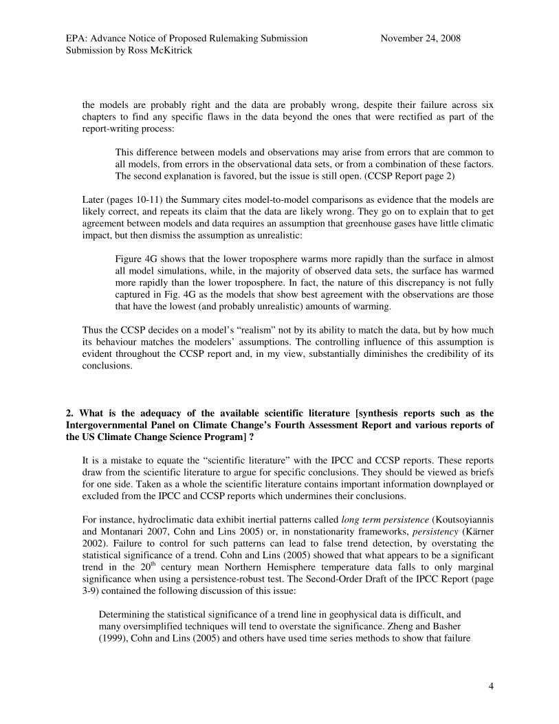
DATA
Weather satellite records for the mid-troposphere are available from Remote Sensing Systems (RSS) in California and the Earth Systems Science Center at the University of Alabama-Huntsville (UAH). I obtained the data from each lab for the mid-troposphere layer covering January 1979 to September 2008. Over this interval the annual average atmospheric concentration of CO2 measured at Mauna Loa Hawaii rose from 337 ppm to 384 ppm (http://cdiac.ornl.gov/ftp/trends/co2/maunaloa.co2), a 14% increase. I have graphed the RSS and UAH tropical mid-troposphere series and compared them to the CCSP- and IPCC-predicted trends (0.25 oC/decade and 0.5 oC/decade respectively).
In contrast to climate model predictions the data indicate neither significant warming in the tropics
nor greater warming than at the poles.
-1-.
50
.51
1.5
Deg
ree
s C
1976m9 1985m1 1993m5 2001m9 2010m1Time period (year.month)
Trpcs projected_ccsp_trend
projected_ipcc_trend
RSS Tropical Mid-Trop vs IPCC and CCSP models
IPCC (A1B) Projection
0.5 oC/decade
CCSP Projection
0.25 oC/decade
Observed (RSS)
APPENDIX A: Response to Hon. Dingell
16
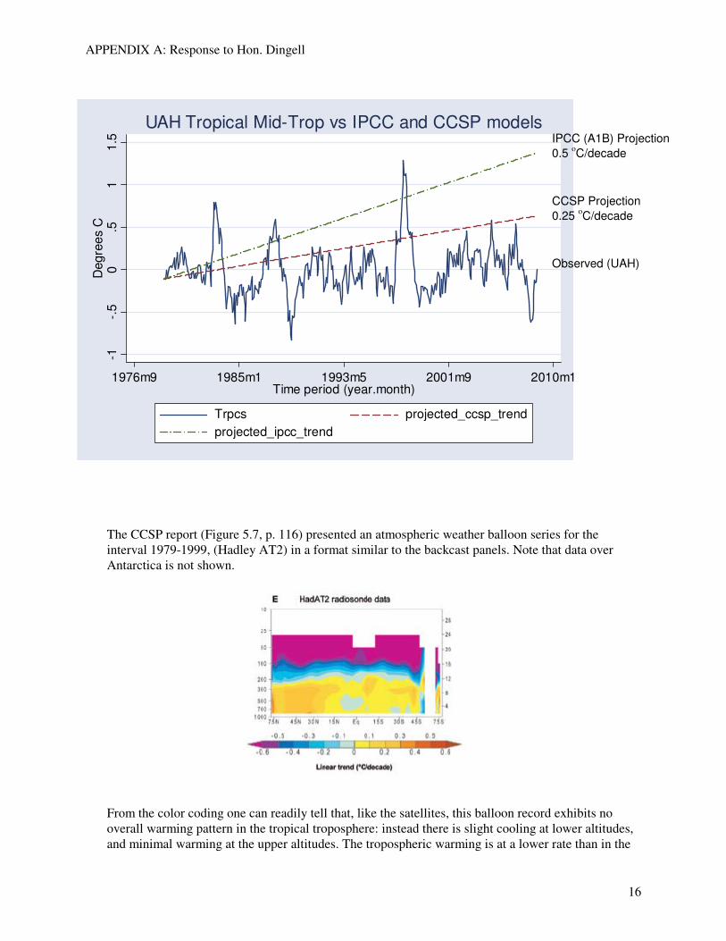
The CCSP report (Figure 5.7, p. 116) presented an atmospheric weather balloon series for the
interval 1979-1999, (Hadley AT2) in a format similar to the backcast panels. Note that data over Antarctica is not shown.
From the color coding one can readily tell that, like the satellites, this balloon record exhibits no
overall warming pattern in the tropical troposphere: instead there is slight cooling at lower altitudes, and minimal warming at the upper altitudes. The tropospheric warming is at a lower rate than in the
-1-.
50
.51
1.5
Deg
ree
s C
1976m9 1985m1 1993m5 2001m9 2010m1Time period (year.month)
Trpcs projected_ccsp_trend
projected_ipcc_trend
UAH Tropical Mid-Trop vs IPCC and CCSP models
IPCC (A1B) Projection
0.5 oC/decade
CCSP Projection
0.25 oC/decade
Observed (UAH)

APPENDIX A: Response to Hon. Dingell
17
troposphere as a whole and lower in comparison to the North Pole region. The CCSP text (fn 66, p. 115) points out that this data span includes the ‘end-point effect’ of the powerful 1998-1999 El Nino so the absence of tropical tropospheric warming is an even more conspicuous discrepancy with the models.
I computed linear trends (in oC/decade) for the most up-to-date RSS and UAH data, which are as
follows. An asterix (*) denotes the trend is statistically significant, i.e. distinguishable from random fluctuations.
Atmospheric Region Remote Sensing Systems University of Alabama
Temperature trend in C/decade, 1979:1 to 2008:9
(Std Error of trend in parentheses)
Globe 0.09* (0.042) 0.04 (0.040)
North Pole 0.25* (0.058) 0.23* (0.058)
Northern Hemisphere 0.15* (0.045) 0.09* (0.040)
Tropics 0.11 (0.074) 0.03 (0.071)
Southern Hemisphere 0.03 (0.036) -0.01 (0.034)
South Pole -0.11 (0.070) -0.12 (0.073)
Temperature trends in mid-troposphere, January 1979 to September 2008. Sources: http://www.remss.com/pub/msu/monthly_time_series/RSS_Monthly_MSU_AMSU_Channel_TMT_Anomalies_Land_and_Ocean_v03_2.txt http://vortex.nsstc.uah.edu/data/msu/t2/uahncdc.mt Trend regression computed using STATA arima(1,0,1) specification: code posted at
http://ross.mckitrick.googlepages.com/S.Dingell.zip.
The satellite data reveal warming in the mid-troposphere over the northern high latitudes but little elsewhere: in particular none over the Southern Hemisphere and a cooling trend at the South Pole. Both satellite series confirm the absence of a significant warming trend in the tropical mid-troposphere.
In both the RSS and UAH data sets there is a slight upward global trend, which in neither case
exceeds 0.1 oC per decade over the past 30 years, despite the addition of 47 ppm CO2 to the atmosphere. This is well below the range of 0.25-0.5 oC/decade predicted by climate models. In both the RSS and UAH series the tropical trend about equals the global trend, whereas models predict it should exceed the global trend and be at least double that over each pole. In neither data set does the tropical region exhibit a larger trend than the North Pole; and in both data sets the South Pole has cooled, opposite to the backcast results in the IPCC and CCSP reports.
The satellite series differ in part because of their treatment of inter-satellite calibration in the early
segment, with the RSS series initially tracking lower than the UAH series, yielding higher trend values over the entire sample. But over the past decade (January 1999 to September 2008) the UAH series has exhibited larger warming trends than the RSS data, and no region exhibits statistically significant warming in either data set. The RSS series since 1999 shows cooling over the Southern

APPENDIX A: Response to Hon. Dingell
18
Hemisphere, and a global trend of only 0.006 oC/decade, despite a 4% rise in atmospheric CO2 over this interval.
The strong warming in the mid-troposphere over the North Pole deserves some comment. Models
predict amplified warming over the North Pole due to an “albedo” effect: as snow and ice melt the reflectivity of the surface declines and more heat is absorbed, increasing the local infrared radiation and the subsequent greenhouse warming. Because the mechanism operates at the surface there is a distinct vertical pattern to it: the GHG-induced warming is supposed to be strongest at the surface, then weaken with altitude.
But a recent paper in Nature (Graversen et al. “Vertical structure of recent Arctic warming, Nature
vol 541, 3 Jan 2008, 53—57) reported that, except in the Spring, the warming is stronger aloft than at the surface, opposite to the expected pattern (in the Spring the warming is uniform up to 700 hPa).
(Fig. 4a, Graversen et al. 2008)
They also noted that amplified North Pole warming is observed in winter months when there is so
little sunshine that the albedo effect cannot be influential. This vertical and seasonal warming structure is inconsistent with the albedo mechanism in climate models. Graversen et al. showed that the trends can largely be explained by variations in atmospheric energy transport, in particular the atmospheric northward energy transport (ANET) index, a measure of wind-borne heat crossing the 60th parallel latitude. The ANET index has increased in recent decades. Graversen et al. do not determine why this is so, but point to its connection with cloud cover, large-scale oscillations and planetary waves. Carbon dioxide may affect these processes but such a connection would be indirect and obscure, and is not represented in climate models. The authors conclude that much of the present
From IPCC Figure 9.1: Models predict GHG warming is strongest at the surface then weakens higher up
Observed summer half-year warming (1979-2001, April-Oct) concentrated in lower troposphere, not at surface

APPENDIX A: Response to Hon. Dingell
19
Arctic warming appears linked to processes other than the albedo-driven greenhouse amplification mechanism in climate models.
Overall, in answer to your question, climate models project that, if greenhouse gases dominate the
climate, the troposphere over the tropics and over both poles should be warming; the tropical troposphere should be warming two to three times faster than the polar tropospheric regions, namely at a rate of about 0.25 to 0.5 oC/decade, and the polar warming should be strongest at the surface. The data, however, do not support any of these hypotheses. They show, at most, a trend of about 0.1 oC/decade in the tropical mid-troposphere, it is statistically insignificant and recently the annual mean temperature has fallen below the level observed in the early 1980s, despite an overall 14% increase in the atmospheric CO2 content since that time. The trend observed in the tropics over the past 30 years is less than half that observed over the North Pole, and the troposphere over the South Pole is cooling, not warming. The enhanced trend over the North Pole has been attributed to variations in atmospheric heat transport, and the vertical structure is inconsistent with the pattern predicted in models as an amplified response to greenhouse gases.
One of my biggest concerns about cap-and-trade systems is that they ask the people of the US to
commit to permanently higher energy costs based global warming forecasts from models that appear systematically to overestimate climate sensitivity to greenhouse gases and hence the environmental costs of emissions. In a subsequent question you ask about pricing in risk, so I will return to this issue below.
4. Your testimony states that carbon taxes can more easily alleviate the regressivity of higher energy
prices (from either a carbon tax or a cap-and-trade system) because offsetting tax reductions can be directed towards low-income houses. Do you agree that, if the Government auctioned all allowances in a cap-and-trade system (instead of giving them away for free) then the Government could address regressivity by directing offsetting tax reductions to low-income households? If you disagree please explain why.
I would agree with this statement if the auction were a one-time event and the demand curve for
permits were not too steep. But what is being proposed is a repeated (annual) event in which a fixed supply of permits is auctioned into a market with a very steep demand curve, the position of which is closely tied to output and energy consumption and which therefore is prone to shift over time. This makes it difficult to forecast the permit price and the resulting revenue from the auction. Therefore the size of the necessary tax reductions cannot be estimated from year to year except with large error.
The diagram below uses the geometry of demand-supply analysis to show a hypothetical example. A
steep demand curve means that relatively large price increases are needed to reduce the quantity demanded. A small error in forecasting the demand for permits (the gap between the dotted and solid demand curves) translates into a large error in the estimate of the permit price. This would cause a correspondingly large error in the estimated total auction revenues and the corresponding estimate of the required compensation for low-income compensation households. Hence it would be difficult to write a budget that commits to compensatory tax cuts of anywhere near the correct magnitude from one year to the next.

APPENDIX A: Response to Hon. Dingell
20
If, however, the policy had taken the form of an emissions tax at the estimated price, the steepness of
the demand curve ensures that, even with the gap between the estimated and actual demand curves, the resulting quantity of emissions would be close to the estimated quantity, and the resulting tax revenues and required compensation for low-income compensation households would be close to the initial estimate. For this reason, budgeting for compensatory tax cuts would be much more feasible under an emissions tax regime.
The demand curve for sulfur permits is not as steep as that for carbon permits, yet the price of US
Acid Rain Allowances has nonetheless been extremely volatile: from July 2005 to January 2006 prices rose from just over $500 to over $1500 per tonne, then fell to below $500 by July 2006, spiking back to over $700 per tonne in July 2007 before retreating to about $550 per tonne in the fall of 2007. We can expect even greater volatility in carbon permit markets unless price guarantees are in place.2
The reason the demand curve for permits is likely very steep is that CO2 control options are very
limited compared to sulfur dioxide. All the reductions in SO2 emissions during the first phase of compliance with the 1990 Clean Air Act Amendments came about through installing scrubbers and switching to low-sulfur sources of the same fuel. But there are no scrubbers for CO2 and there is no “low-carbon” version of coal or oil. The only large-scale CO2 abatement options, for the foreseeable future, are to reduce energy consumption or switch to different fuel types, which are very costly at the margin. This translates into a steep demand curve, i.e. a likelihood of rapidly increasing bid prices for permits.
2 See http://www.chicagoclimatex.com/news/publications/pdf/CCXQ_Spr06.pdf and http://www.chicagoclimatex.com/docs/publications/CCFE_sulfurmkt_V4_i11_nov2007.pdf
Quantity of permits
Price of permits
Supply fixed by law
Estimated demand curve
Actual Demand Curve
Actual price
Estimated price

APPENDIX A: Response to Hon. Dingell
21
5. Your testimony states that, in the economics literature, marginal cost estimates of greenhouse gases
are in the range of $20 a tonne of CO2 –equivalent. Do these estimates put a dollar value on loss of ecosystems or species extinction? If so, please explain.
Yes, some studies do, though the methodologies differ. For example, Hope (2006) uses the
PAGE2002 Integrated Assessment Model (the same one used for the Stern Review) and embeds valuation for risks to unique and threatened ecosystems as well as the possibility of abrupt or extreme events. This study yielded a marginal damage estimate of about US$5 per tonne of CO2 (or US$19 per tonne of carbon). Also, as discussed in the Stern Review (Chapter 6 pp. 147—148) the models of Tol and Nordhaus include ecosystem changes.
The Stern Review obtained much higher numbers using the Page2002 model by programming in very
high climate sensitivity parameters, and adding in new damage categories of a rather speculative nature, most of which do not begin to accumulate in the model until some time in the 22nd century. Then, by using a very low discount rate, high damages occurring 100 to 200 years from now are valued as being nearly equivalent to damages today. The Stern Review justified using high sensitivity parameters by referring to what it considers to be an increasing probability of global warming occurring at a rate of 5—6 oC/century (e.g. p. 151). A surface warming rate of 5—6 oC/century would imply warming in the tropical troposphere of approximately 1.0—1.2 oC/decade, some 10 times the actual, observed rate. The Stern Review does not explain how it concluded this outcome has become more likely even though the available data shows the opposite.
Reference: Hope, C (2006). “The Marginal Impact of CO2 from PAGE2002: An Integrated
Assessment Model Incorporating the IPCC’s Five Reasons for Concern.” The Integrated Assessment Journal 6(1) 19—56.
6. Multiple leading scientists have warned us of potential “threshold” effects of climate change, where
various temperature increases can provoke sudden and potentially self-reinforcing swings in environmental stability. One such example would be large-scale melting of the permafrost, which would release even more potent methane emissions. Another would be the collapse of Greenland and Antarctica ice sheets over land, which could dramatically raise sea level. How, if at all, does a marginal estimate of the value of any particular single tonne of CO2 take the risk of surpassing these tipping points into account?
Integrated Assessment Models attempt to price in the possibility of a dramatic climate change in
much the same way as investment models try to price in the possibility of major default or other calamity: by adding a “risk premium” to the price based on the wideness of the range of possible outcomes and the losses or gains associated with extreme events. If it were known that damages due to global warming had a mean value of, say, $10, the appropriate emissions price would be different if the possible range were -$20 to +$250 as opposed to $5 to $15. If we had to commit now to an emissions price, we would need to add a premium to the price in the former case to account for the risk that the damages might be far higher than forecast.
If a study appears in the literature that points to the possibility of abrupt or extreme climate change
causing trillions of dollars in future damages, it does not mean the risk premium should automatically increase. It depends on how likely the scenario is and how credible the numbers are. That is why

APPENDIX A: Response to Hon. Dingell
22
Tol’s surveys include efforts to assess the credibility of the study, based on whether it was peer reviewed, what discount rate was applied, and so forth.
I don’t find these points very satisfactory as an answer to your question, however. The reality is that
nobody can forecast major, abrupt climate changes, but if such events are possible, the cost of trying to prevent them through elimination of fossil fuel use would be extraordinarily high. Hence you and your colleagues must weigh uncertain warnings of massive ecological dangers against the more certain matter that the putative remedies would cause massive economic dangers. I do not believe that the science (such as it is) of computing risk premiums is the right tool for sorting this out. Instead, in my testimony I drew attention to the need to use what we call state-contingent strategies, which build into the policy framework a direct feedback between the observed severity of the problem and the stringency of the policy. If done right, a feedback mechanism would help you avoid the costs of taking too much or too little action by tying the emissions price (or cap) to the actual amount of warming that is observed.
None of the proposals before Congress do this. Instead they try to strike an impossible compromise
between supporters of aggressive controls on CO2 emissions who fear that weak targets will not be tightened in the future even if the situation looks more and more dangerous, and opponents of action who fear that restrictions on CO2 will become an unchangeable status quo even if global warming is decisively refuted over the coming decade (as I expect it will be).
A risk premium formula cannot solve this dilemma, no matter how complex the calculations are. But
a simple feedback (or state-contingent) mechanism can. For a cap and trade system it would work as follows. Since 1960, US greenhouse gas emissions intensity declined, on average by about 1.7% per year, while the US economy grew, on average, by about 3% per year. So without any regulation, if global warming were not an issue, you would expect an average increase in greenhouse gas emissions of about 1.3% per year. Now suppose we impose the following requirements on any emissions cap rule:
» If, as of 2010, the IPCC mid-range (A1B) scenario is true, the cap should decline by 35% between
2010 and 2030, in line with many of the proposals before Congress. » If the Stern Review worst-case scenario is true (1 oC/decade in the tropical troposphere) the
emissions cap should fall by 95% by 2030. » If there is no trend in the mean temperature of the tropical troposphere between 2010 and 2030,
the cap on emissions should grow by 1.3% per year. » If the tropical troposphere starts cooling in 2010 the allowed emissions level could rise faster than
1.3% per year. » If there is a sudden increase in global average temperatures the cap should suddenly tighten in
response. The formula that yields this outcome is CAP(t+1) = CAP(t) + 0.013 - (CHANGE x 0.61) (1) where CAP(t) is the cap in year t, expressed as the fraction of 2010 emissions, CHANGE is the
observed change per year in the mean temperature of the tropical troposphere from RSS or UAH (or both, averaged), and 0.61 is the number needed to yield the desired slopes. As of 2030, CAP would equal 0.65 (i.e. a 35% emissions reduction) if the A1B warming rate is observed after 2010, it would equal 0.04 (i.e. a 96% emissions reduction) if the Stern “High Sensitivity” rate is observed, it would

APPENDIX A: Response to Hon. Dingell
23
equal 1.26 if there is no warming trend, and it would rise to 1.38 if there is a 0.1 oC/decade cooling trend. The paths look as follows.
Allowable Emissions If Cap is Tied to Actual Warming
0.00
0.20
0.40
0.60
0.80
1.00
1.20
1.40
1.60
2010 2015 2020 2025 2030
Year
Fra
cti
on
of
201
0 E
mis
sio
ns
IPCC-A1B (0.5 C/decade)
Stern (1 C/decade)
No Trend
Cooling (0.1 C/decade)
By tying the cap to the actual warming rate it ensures you end up with the most appropriate outcome
regardless of whose forecast is right. It would also force the private sector to make an unbiased assessment of the credibility of different forecasts and invest based on which ones are consistently the most accurate, since the actual abatement targets will depend on actual warming, not model forecasts.
Someone who believes in a Stern-type future would have every reason to support this formula since
they would expect it to yield radically reduced greenhouse gas emissions over the next two decades. Likewise, someone who dismisses the possibility of global warming altogether should equally support this formula since they would expect the emissions cap to rise fast enough to ensure a permit price of zero. Hence the state-contingent approach avoids the political fight associated with trying to estimate a risk premium.
Tying the emissions cap to actual warming also provides a constructive way of dealing with the
threat of abrupt climate changes, or “tipping points.” If the future path of warming is minimal for a while, then suddenly switches to an abrupt warming trend, the above formula would instantly tighten the allowable emissions. More importantly, if science progressed to the point where such a change could be reliably forecast, then emitters would begin planning on higher permit prices as far in advance as the forecast could be made. Of course if science never permits such forecasts then no policy will anticipate them, but my suggestion will at least ensure a rapid, automatic response. If no such abrupt change ever takes place, then the feedback rule would avoid imposing unnecessarily the costs associated with trying to prevent it.
The chief objection to a feedback-based approach is that it seems to be backward-looking, taking
action only after the problem has been revealed, yet warming may not happen right away in response to greenhouse gases. However, according to the IPCC, the tropical troposphere (in models) adjusts rapidly to changes in greenhouse gas changes, making it an appropriate metric for guiding changes in the cap. Also, investors and firms are forward-looking: they make decisions now based on expected market conditions years ahead. By tying the carbon dioxide emissions control policy to contemporary

APPENDIX A: Response to Hon. Dingell
24
atmospheric conditions, it requires firms to take account of the best available climatic data and warming forecasts when making major investment decisions, which is precisely the goal of any long term policy.
Finally, another potential objection to the feedback approach is the fear that emissions today might
commit us to warming a long way ahead, i.e. 20 or 30 years. However, those making this objection are asking us to trust climate models over actual data. The data show that models have demonstrated insufficient fidelity to the relevant data over the past 30 years to merit trusting them as the basis for a permanent commitment to reducing American energy consumption over the next 30 years. They consistently over-estimate tropospheric warming and project a spatial pattern that does not match the data. A feedback rule like the one I propose takes the models seriously enough to admit the possibility that greenhouse gases may need to be reduced in the coming years, but hedges that bet by ensuring the policy only gets stringent to the extent the problem is revealed to be serious.
Yours truly,
Ross McKitrick Associate Professor of Economics

APPENDIX B: Response to Sen. Inhofe
DEPARTMENT OF ECONOMICS College of Management and Economics University of Guelph Guelph Ontario, Canada N1G 2M5 (519) 824-4120 Ext. 52532 http://www.uoguelph.ca/~rmckitri/ross.html [email protected]
Ross McKitrick, Ph.D. Associate Professor and Director of Graduate Studies November 18, 2008 Senator James M. Inhofe Ranking Member Senate Committee on Environment and Public Works Dear Senator Inhofe Thank you for the opportunity to provide some information pertaining to the formulation of climate policy. Your questions, and my answers, are as follows. 1. As policymakers, it is our duty to ensure that models developed by the [Environmental Protection] Agency are useful for their intended purpose, articulate major assumptions and uncertainties, and separate scientific conclusions from policy judgments. Are the models and data relied on by the U.S. Climate Change Science Program and IPCC transparent and verifiable? Can you please comment on their transparency, including for example: whether they have been subject to credible, objective peer review and sensitivity and uncertainty analyses?
The models are superficially transparent because expert users can examine the code. However they are very complex, so their behaviour is not always comprehensible. The 4th IPCC Report, Working Group I (AR4 p. 594) notes:
A climate model is a very complex system, with many components. The model must of course be tested at the system level, that is, by running the full model and comparing the results with observations. Such tests can reveal problems, but their source is often hidden by the model’s complexity.
When models become “black boxes” that nobody can fully understand, direct transparency becomes impossible. At that point we rely on modelers to subject their models to full stress testing and to report the results without trying to conceal any problems exposed by the testing. It is essential that models not merely be “validated”—i.e. the tests cannot simply be designed to look for points of agreement with the data, but must seek out and rectify problems. Where assumptions and structures are refuted, they must either be corrected or the models discarded. Hence the question of model transparency and testing is as much about the communication of testing results to potential users of the model outputs. To put the current issue into perspective, the United

APPENDIX B: Response to Sen. Inhofe
26
States and, indeed, the rest of the world, is now experiencing a devastating economic contraction following the destruction of trillions dollars worth of American and European financial wealth through collapsing asset prices. A substantial part of the blame can be placed on a systemic failure to properly test the pricing models used to evaluate mortgage-backed securities and their derivatives. In a recent analysis of the global financial crisis, Canadian economist Frank Milne3 observes that this came down, in part, to a failure of due diligence by users of the model outputs:
Exuberance, naivety and the lure of large returns allowed many investors to overlook the limits of the models they were relying on, ignore the warning signals by central banks and others, and to skimp on their own due diligence. As the US housing market began to decline, the assumptions and empirical calibration of those models, and the construction of credit instruments and their packaging came into question. Lack of transparency became an increasing issue and liquidity in the relevant markets largely disappeared, as buyers refused to buy these instruments except at deep discounts. The real problem was not so much a lack of short-term liquidity, but very serious informational deficiencies compounded by a lack of transparency and trust. Many [financial institutions] began to worry about the solvency of, and their exposure to, other [financial institutions]. The resulting crisis is having serious consequences for the US real economy, especially housing and consumer durable markets. Policy needs to address problems in US financial markets… If it is not successful, then there are concerns that their problems will multiply and spread internationally into a major systemic credit crisis that will cause a serious international recession.
I see many parallels between the economic crisis induced by an investment bubble in assets that had been systematically over-priced by financial models, and the disputes over how much nations should invest in green energy schemes and other greenhouse gas policies based on climate models that systematically over-predict the effects of carbon dioxide emissions. In hindsight we now know that we should have been far more skeptical about computerized financial models, we should not have assumed that because they all produced similar outputs they must all therefore be correct, we should not have assumed that the eminence of the professors who developed them ruled out the possibility that they could be fundamentally flawed, and we should have paid attention to the discrepancies between their structural features and observed reality (e.g. concerning liquidity of some asset markets). We should also have listened to those few isolated individuals who tried to warn international leaders that the “consensus” of financial experts masked serious problems of groupthink and blind momentum. Likewise, skepticism about climate models must be strongly encouraged and where serious problems are identified, the models must be fixed or rejected. Yet skepticism about climate models is nowhere to be found in the prominent summaries coming from the IPCC and the Climate Change Science Program (CCSP). The CCSP report of June 2006 (Temperature Trends in the Lower Atmosphere: Steps for Understanding and Reconciling Differences) provides a striking example of this. In the Executive Summary the report describes a “potentially serious inconsistency” (p. 11) between model predictions and observed data in the tropical troposphere. All models predict amplified warming in the tropical troposphere as an essential component of the assumed greenhouse gas-induced global warming mechanism. Yet the numerous data sets analysed and scrutinized in the CCSP report fail to
3 Milne, Frank (2008) “Anatomy of the Credit Crisis: The Role of Faulty Risk Management Systems”
C.D. Howe Institute Commentary No. 269, July 2008.
APPENDIX B: Response to Sen. Inhofe
27
show this pattern. Rather than acknowledge that the models appear to be wrong, the CCSP report claims that the models are probably right and the data are probably wrong, despite their failure across six chapters to find any specific flaws in the data beyond the ones that were rectified as part of the report-writing process:
This difference between models and observations may arise from errors that are common to all models, from errors in the observational data sets, or from a combination of these factors. The second explanation is favored, but the issue is still open. (CCSP Report page 2)
Later (pages 10-11) the Summary cites model-to-model comparisons as evidence that the models are likely correct, and repeats its claim that the data are likely wrong. They go on to explain that to get agreement between models and data requires an assumption that greenhouse gases have little climatic impact, but then dismiss the assumption as unrealistic:
Figure 4G shows that the lower troposphere warms more rapidly than the surface in almost all model simulations, while, in the majority of observed data sets, the surface has warmed more rapidly than the lower troposphere. In fact, the nature of this discrepancy is not fully captured in Fig. 4G as the models that show best agreement with the observations are those that have the lowest (and probably unrealistic) amounts of warming.
Thus the CCSP decides on a model’s “realism” not by its ability to match the data, but by how much its behaviour matches the modelers’ assumptions. The controlling influence of this assumption is evident throughout the CCSP report and, in my view, substantially diminishes the credibility of its conclusions. The main tool for testing any kind of model is to examine its accuracy in reproducing past events, and to show on theoretical grounds that such fidelity implies accuracy in forecasting. Considering the magnitude of the policy decisions resting on climate model output, it is important to note the IPCC’s admission that this kind of testing has barely begun:
What does the accuracy of a climate model’s simulation of past or contemporary climate say about the accuracy of its projections of climate change? This question is just beginning to be addressed, exploiting the newly available ensembles of models….the development of robust metrics is still at an early stage. (AR4 Working Group I pp. 594-5).
In the Second Order Draft of the 4th IPCC Report (AR4), at the close of scientific review (June 2006) the text stated that even models tuned to “perfectly” reproduce the observed climate did not necessarily have predictive ability.
[P]reliminary studies relying on “perfect model” simulations (e.g., Murphy et al., 2004; Stainforth et al., 2005) show only a weak relationship between certain measures of model skill in simulating climatology and the accurate prediction of future climate, so at this time it is impossible to establish minimum threshold criteria that models must meet to be trusted as reliable prediction tools. Nevertheless, poor model skill in simulating present climate indicates that certain physical processes have been misrepresented. (Working Group I Second Draft, page 8-18).

APPENDIX B: Response to Sen. Inhofe
28
This paragraph was heavily edited prior to release of the published version, as follows
[P]reliminary studies relying on “perfect model” simulations (e.g., Murphy et al., 2004; Stainforth et al., 2005) show only a weak relationship between certain measures of model skill in simulating climatology and the accurate prediction of future climate, so at this time it is impossible to establish minimum threshold criteria that models must meet to be trusted as reliable prediction tools. Poor model skill in simulating present climate indicates could indicate that certain physical or dynamical processes have been misrepresented. (Working Group I Report, page 608).
While the IPCC makes some effort to evaluate their models, and they counsel caution in using model results, they have not identified whether their models can be or have been falsified, and even downplay the idea of such testing. For instance, on page 594 of the Working Group I contribution to the AR4, they state:
A specific prediction based on a model can often be demonstrated to be right or wrong, but the model itself should always be viewed critically. This is true for both weather prediction and climate prediction. Weather forecasts are produced on a regular basis, and can be quickly tested against what actually happened. Over time, statistics can be accumulated that give information on the performance of a particular model or forecast system. In climate change simulations, on the other hand, models are used to make projections of possible future changes over time scales of many decades and for which there are no precise past analogues. Confidence in a model can be gained through simulations of the historical record, or of palaeoclimate, but such opportunities are much more limited than are those available through weather prediction.
Notice that they only describe a process that builds confidence in models, without specifying circumstances in which climate models can might actually be refuted. In the body of the IPCC AR4 there are numerous warnings about the limited accuracy of climate models, but these were omitted from the Summary for Policymakers. Section 8.1.3.1 cautions that fundamental climatic processes are represented in models by approximations that may have little or no empirical basis, and that there has been no formal evaluation of whether models are “overfit” against the data, which would mean their fidelity to observed climate conditions is meaningless as a test of forecast skill:
Parametrizations are typically based in part on simplified physical models of the unresolved processes (e.g., entraining plume models in some convection schemes). The parametrizations also involve numerical parameters that must be specified as input. Some of these parameters can be measured, at least in principle, while others cannot. It is therefore common to adjust parameter values (possibly chosen from some prior distribution) in order to optimise model simulation of particular variables or to improve global heat balance. This process is often known as ‘tuning’. It is justifiable to the extent that two conditions are met: 1. Observationally based constraints on parameter ranges are not exceeded. Note
that in some cases this may not provide a tight constraint on parameter values (e.g., Heymsfield and Donner, 1990).

APPENDIX B: Response to Sen. Inhofe
29
2. The number of degrees of freedom in the tuneable parameters is less than the
number of degrees of freedom in the observational constraints used in model evaluation. This is believed to be true for most GCMs – for example, climate models are not explicitly tuned to give a good representation of North Atlantic Oscillation (NAO) variability – but no studies are available that formally address the question. If the model has been tuned to give a good representation of a particular observed quantity, then agreement with that observation cannot be used to build confidence in that model.
(Working Group I Report p. 596).
They also warn that cloud processes are highly influential on model results, yet are poorly represented in models and it is not yet possible to resolve the differences among models:
Recent studies reaffirm that the spread of climate sensitivity estimates among models arises primarily from inter-model differences in cloud feedbacks. The shortwave impact of changes in boundary-layer clouds, and to a lesser extent mid-level clouds, constitutes the largest contributor to inter-model differences in global cloud feedbacks. The relatively poor simulation of these clouds in the present climate is a reason for some concern. The response to global warming of deep convective clouds is also a substantial source of uncertainty in projections since current models predict different responses of these clouds. Observationally based evaluation of cloud feedbacks indicates that climate models exhibit different strengths and weaknesses, and it is not yet possible to determine which estimates of the climate change cloud feedbacks are the most reliable. (Working Group I Report p. 593).
These are all germane points, and imply that the results of climate modeling (including attribution of past warming to greenhouse gases as well as predictions of future warming) are inherently uncertain and tentative. But none of this went into the Summary for Policymakers, whose only comment on model assessment was:
Advances in climate change modelling now enable best estimates and likely assessed uncertainty ranges to be given for projected warming for different emission scenarios. (SPM page 13, emphasis in original)
This is clearly an inadequate summary of the situation, to the point of being misleading. Hence, in response to the first question, the IPCC Report indicates that rigorous, objective assessment of model accuracy is only at an early stage, and that there are major limitations and deficiencies in climate models, but this information was omitted from the IPCC’s Summary for Policymakers.
2. There has been increasing concern among climatologists and statisticians that existing models have limited abilities in predicting localized effects. In your professional opinion, how accurate are the global models at mimicking atmospheric processes as they relate to effects on local climates?

APPENDIX B: Response to Sen. Inhofe
30
The key testing ground for climate models is their prediction concerning amplified warming in the troposphere over the tropics. Held and Soden (2000, p. 471)4 discuss the importance of observing an accumulation of water vapor in the tropical troposphere as follows:
Given the acceleration of trends predicted by many models, we believe that an additional 10 years may be adequate, and 20 years will very likely be sufficient, for the combined satellite and radiosonde network to convincingly confirm or refute the predictions of increasing vapor in the free troposphere and its effects on global warming.
It is now 10 years since they wrote that statement. Yet rather than squarely facing up to the possible falsification of climate models by reporting tests of models against the tropical troposphere, the IPCC repeatedly compares model outputs to surface data. The surface data are known to be biased due to land-use modification and other sources of artificial warming.5 There is clear evidence of an upward bias, especially after 1980, in global land surface temperature records due to well-documented data quality problems. This should be borne in mind when examining the striking Figure on page 11 of the IPCC Summary for Policymakers (see below) which they present as evidence of greenhouse gas-induced warming. The Figure shows a divergence between model-generated estimates of averaged land surface temperatures after 1980 without greenhouse gas effects (blue band) and with greenhouse gas effects (red band); and the latter neatly overlaps the temperature record (black line). This is the basis for their claim that greenhouse gas effects have caused the observed warming.
4 Held, I. and B. J. Soden (2000) “Water Vapor Feedback and Global Warming” Annual Review of Energy and
Environment 25:441—75. 5 Pielke R.A. Sr., G. Marland, R.A. Betts, T.N. Chase, J.L. Eastman, J.O. Niles, D.D.S. Niyogi and S.W. Running.
(2002) “The Influence of Land-use Change and Landscape Dynamics on the Climate System: Relevance to Climate-Change Policy Beyond the Radiative Effect of Greenhouse Gases.” Philosophical Transactions of the Royal Society
of London. A360:1705-1719; McKitrick, R and P. J. Michaels (2004). “A Test of Corrections for Extraneous Signals in Gridded Surface Temperature Data” Climate Research 26(2) pp. 159-173. “Erratum,” Climate Research 27(3) 265—268. McKitrick, Ross R. and P.J. Michaels (2007) “Quantifying the influence of anthropogenic surface processes and inhomogeneities on gridded global climate data.” Journal of Geophysical Research, 112, D24S09, doi:10.1029/2007JD008465, 2007; De Laat, A.T.J., and A.N. Maurellis (2004). “Industrial CO2 Emissions as a Proxy for Anthropogenic Influence on Lower Tropospheric Temperature Trends.” Geophysical Research Letters Vol. 31, L05204, doi:10.1029/2003GL019024. De Laat, A.T.J., and A.N. Maurellis (2006). “Evidence for Influence of Anthropogenic Surface Processes on Lower Tropospheric and Surface Temperature Trends.” International Journal of Climatology 26:897—913.

APPENDIX B: Response to Sen. Inhofe
31
IPCC Summary for Policymakers page 11.
The blue and red bands diverge after about 1980. The blue band is generated by considering only solar changes and volcanic events as represented in the models. The red band is generated by adding a strong greenhouse gas warming effect. What they do not show is a case in which the model is run with natural forcings plus land surface modifications, urbanization and other data contamination problems, but little or no greenhouse gas warming. Depending on parameter choices this could also generate a band like the red one. Hence the presentation of modeling results in the Summary for Policymakers proves nothing, it is simply a selective and promotional insinuation. Turning to the question of model fidelity in the troposphere, this issue is passed over in the Summary for Policymakers with the following claim (Summary for Policymakers p. 10)
Warming of the climate system has been detected in changes of surface and atmospheric temperatures in the upper several hundred metres of the ocean, and in contributions to sea level rise. Attribution studies have established anthropogenic contributions to all of these changes. The observed pattern of tropospheric warming and stratospheric cooling is very likely due to the combined influences of greenhouse gas increases and stratospheric ozone depletion. {3.2, 3.4, 9.4, 9.5}
I will make one brief comment about the stratosphere, but otherwise confine my comments to the tropospheric record. The stratospheric record from Remote Sensing Systems in California looks as follows:
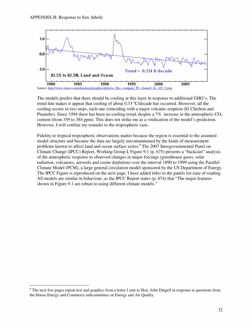
APPENDIX B: Response to Sen. Inhofe
32
Source: http://www.remss.com/data/msu/graphics/plots/sc_Rss_compare_TS_channel_tls_v03_2.png
The models predict that there should be cooling at this layer in response to additional GHG’s. The trend line makes it appear that cooling of about 0.33 oC/decade has occurred. However, all the cooling occurs in two steps, each one coinciding with a major volcanic eruption (El Chichon and Pinatubo). Since 1994 there has been no cooling trend, despite a 7% increase in the atmospheric CO2 content (from 359 to 384 ppm). This does not strike me as a vindication of the model’s prediction. However, I will confine my remarks to the tropospheric case.
Fidelity to tropical tropospheric observations matter because the region is essential to the assumed model structure and because the data are largely uncontaminated by the kinds of measurement problems known to affect land and ocean surface series.6 The 2007 Intergovernmental Panel on Climate Change (IPCC) Report, Working Group I, Figure 9.1 (p. 675) presents a “backcast” analysis of the atmospheric response to observed changes in major forcings (greenhouse gases, solar radiation, volcanoes, aerosols and ozone depletion) over the interval 1890 to 1999 using the Parallel Climate Model (PCM), a large general circulation model sponsored by the US Department of Energy. The IPCC Figure is reproduced on the next page. I have added titles to the panels for ease of reading. All models are similar in behaviour, as the IPCC Report states (p. 674) that “The major features shown in Figure 9.1 are robust to using different climate models.”
6 The next few pages repeat text and graphics from a letter I sent to Hon. John Dingell in response to questions from the House Energy and Commerce subcommittee on Energy and Air Quality.

APPENDIX B: Response to Sen. Inhofe
33
The format of each panel is as follows. Latitude goes from left to right, with the North Pole at the
left, the equator in the middle and the South Pole at the right. Altitude is on the vertical axis, beginning at the surface and rising through the troposphere and into the stratosphere. The colour represents the predicted temperature change in response to the forcing. Dark blue and purple represent strong cooling. As the shading moves through light blue, light yellow and into orange and red the implied temperature change moves upwards towards strong warming.
I have added a horizontal line in the Greenhouse Gases panel indicating the approximate height of
the mid-troposphere: just over 8 km at the poles, rising to about 12 km in the tropics. As is clear from the coloring gradient, the model troposphere over the tropics shows greater
sensitivity to greenhouse gas accumulation than does the troposphere over the polar region. The color tones indicate that, in response to 20th century greenhouse gas accumulation, the model says there ought to have been a warming rate of over 1 C per century in the troposphere over the tropics, and
Solar Volcanoes
Greenhouse gases Ozone
Sulfate aerosols TOTAL
Mid-troposphere
From 2007 IPCC Report page 675
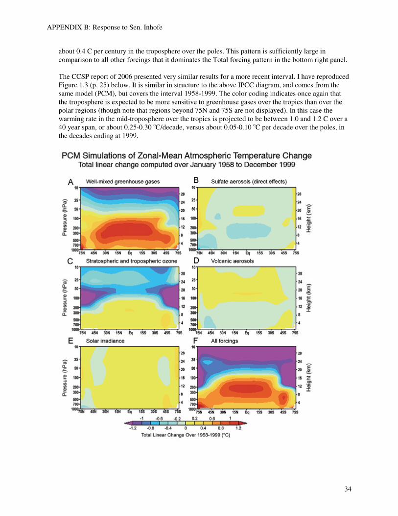
APPENDIX B: Response to Sen. Inhofe
34
about 0.4 C per century in the troposphere over the poles. This pattern is sufficiently large in comparison to all other forcings that it dominates the Total forcing pattern in the bottom right panel.
The CCSP report of 2006 presented very similar results for a more recent interval. I have reproduced
Figure 1.3 (p. 25) below. It is similar in structure to the above IPCC diagram, and comes from the same model (PCM), but covers the interval 1958-1999. The color coding indicates once again that the troposphere is expected to be more sensitive to greenhouse gases over the tropics than over the polar regions (though note that regions beyond 75N and 75S are not displayed). In this case the warming rate in the mid-troposphere over the tropics is projected to be between 1.0 and 1.2 C over a 40 year span, or about 0.25-0.30 oC/decade, versus about 0.05-0.10 oC per decade over the poles, in the decades ending at 1999.

APPENDIX B: Response to Sen. Inhofe
35
Turning now to projections of the climatic response to future increases in greenhouse gases, I have reproduced below one of the 12 climate model projections used for Figure 10.7 of the IPCC Report (p. 765). The models show the response to the A1B emissions scenario, which is in the middle of the group of IPCC climate simulations (see IPCC Figure 10.4). All 12 model runs are available on-line at http://ipcc-wg1.ucar.edu/wg1/Report/suppl/Ch10/Ch10_indiv-maps.html. The printed version of Figure 10.7 uses stippling to show the uniformity of results across models, but this makes it harder to see the color gradients, so I have selected the output from a single model, the Goddard Institute of Space Studies (GISS) model EH, for increased clarity.
The panels in the top row are each in the same format as those in the PCM diagrams above, except
that, going from left to right, latitude runs from South to North, and the vertical axes do not extend as far up into the stratosphere. The bottom three panels show projected oceanic changes.
Source: http://ipcc-wg1.ucar.edu/wg1/Report/suppl/Ch10/indiv_maps/html/GISS-EH_10.7.html The color coding indicates, over the indicated interval, the predicted change in the mean temperature
compared to the observed mean temperature over the 1980 to 1999 interval. As before, the mid-troposphere over the tropics (300-200hPa) is projected to be more sensitive to increased greenhouse gas levels than the troposphere over the polar regions, in all time intervals. The accompanying IPCC text (pp. 764-765) states:
Upper-tropospheric warming reaches a maximum in the tropics and is seen even in the
early-century time period. The pattern is very similar over the three periods, consistent with the rapid adjustment of the atmosphere to the forcing. These changes are simulated with good consistency among the models.
As of the 2011-2030 interval the troposphere over the tropics is projected to be about 1.5 oC warmer
than the average temperature over the 1980 to 1999 interval. Comparing interval midpoints (1990, 2020) this implies a current average warming of 0.5 oC per decade, noting once again the statement in the IPCC text that this change should be observed even in the early-century time period.

APPENDIX B: Response to Sen. Inhofe
36
To summarize thus far, all the models which have been used for the IPCC and CCSP reports embed parameterizations that yield the following predictions:
» The troposphere over the tropics should exhibit greater warming (more than double the rate) than
the troposphere over the polar regions. » The effects induced by greenhouse gases are so large relative to other forcings (positive and
negative) that the total pattern is predominantly a reflection of the contribution of greenhouse gases.
» The tropical troposphere should have been heating up at a rate of at least 0.25 oC/decade over the past few decades in response to historical greenhouse gas emissions. A middle-range warming projection scenario in the IPCC report predicts warming of about 0.5 oC/decade should now be observable in the tropical mid-troposphere.
Since the models make such consistent predictions there is obvious interest in comparing model
outputs to the available data: a comparison conspicuously absent from the IPCC Summary for Policymakers. Fortunately the data from weather satellites now spans nearly 30 years and is adequate to assess the model predictions.
Weather satellite records for the mid-troposphere are available from Remote Sensing Systems (RSS)
in California and the Earth Systems Science Center at the University of Alabama-Huntsville (UAH). I obtained the data from each lab for the mid-troposphere layer covering January 1979 to September 2008. Over this interval the annual average atmospheric concentration of CO2 measured at Mauna Loa Hawaii rose from 337 ppm to 384 ppm (http://cdiac.ornl.gov/ftp/trends/co2/maunaloa.co2), a 14% increase. I have graphed the RSS and UAH tropical mid-troposphere series and compared them to the CCSP- and IPCC-predicted trends (0.25 oC/decade and 0.5 oC/decade respectively).
-1-.
50
.51
1.5
Deg
ree
s C
1976m9 1985m1 1993m5 2001m9 2010m1Time period (year.month)
Trpcs projected_ccsp_trend
projected_ipcc_trend
RSS Tropical Mid-Trop vs IPCC and CCSP models
IPCC (A1B) Projection
0.5 oC/decade
CCSP Projection
0.25 oC/decade
Observed (RSS)

APPENDIX B: Response to Sen. Inhofe
37
In contrast to climate model predictions the data indicate neither significant warming in the tropics nor greater warming than at the poles.
The CCSP report (Figure 5.7, p. 116) presented an atmospheric weather balloon series for the interval 1979-1999, (Hadley AT2) in a format similar to the backcast panels. Note that data over Antarctica is not shown.
-1-.
50
.51
1.5
Deg
ree
s C
1976m9 1985m1 1993m5 2001m9 2010m1Time period (year.month)
Trpcs projected_ccsp_trend
projected_ipcc_trend
UAH Tropical Mid-Trop vs IPCC and CCSP models
IPCC (A1B) Projection
0.5 oC/decade
CCSP Projection
0.25 oC/decade
Observed (UAH)

APPENDIX B: Response to Sen. Inhofe
38
From the color coding one can readily tell that, like the satellites, this balloon record exhibits no overall warming pattern in the tropical troposphere: instead there is slight cooling at lower altitudes, and minimal warming at the upper altitudes. The tropospheric warming is at a lower rate than in the troposphere as a whole and lower in comparison to the North Pole region. The CCSP text (fn 66, p. 115) points out that this data span includes the ‘end-point effect’ of the powerful 1998-1999 El Nino so the absence of tropical tropospheric warming is an even more conspicuous discrepancy with the models.
I computed linear trends (in oC/decade) for the most up-to-date RSS and UAH data, which are as
follows. An asterix (*) denotes the trend is statistically significant, i.e. distinguishable from random fluctuations.
Atmospheric Region Remote Sensing Systems University of Alabama
Temperature trend in C/decade, 1979:1 to 2008:9
(Std Error of trend in parentheses)
Globe 0.09* (0.042) 0.04 (0.040)
North Pole 0.25* (0.058) 0.23* (0.058)
Northern Hemisphere 0.15* (0.045) 0.09* (0.040)
Tropics 0.11 (0.074) 0.03 (0.071)
Southern Hemisphere 0.03 (0.036) -0.01 (0.034)
South Pole -0.11 (0.070) -0.12 (0.073)
Temperature trends in mid-troposphere, January 1979 to September 2008. Sources: http://www.remss.com/pub/msu/monthly_time_series/RSS_Monthly_MSU_AMSU_Channel_TMT_Anomalies_Land_and_Ocean_v03_2.txt http://vortex.nsstc.uah.edu/data/msu/t2/uahncdc.mt Trend regression computed using STATA arima(1,0,1) specification: code posted at
http://ross.mckitrick.googlepages.com/S.Dingell.zip.
The satellite data reveal warming in the mid-troposphere over the northern high latitudes but little elsewhere: in particular none over the Southern Hemisphere and a cooling trend at the South Pole. Both satellite series confirm the absence of a significant warming trend in the tropical mid-troposphere.
In both the RSS and UAH data sets there is a slight upward global trend, which in neither case
exceeds 0.1 oC per decade over the past 30 years, despite the addition of 47 ppm CO2 to the atmosphere. This is well below the range of 0.25-0.5 oC/decade predicted by climate models. In both the RSS and UAH series the tropical trend about equals the global trend, whereas models predict it should exceed the global trend and be at least double that over each pole. In neither data set does the tropical region exhibit a larger trend than the North Pole; and in both data sets the South Pole has cooled, opposite to the backcast results in the IPCC and CCSP reports.
The satellite series differ in part because of their treatment of inter-satellite calibration in the early
segment, with the RSS series initially tracking lower than the UAH series, yielding higher trend values over the entire sample. But over the past decade (January 1999 to September 2008) the UAH

APPENDIX B: Response to Sen. Inhofe
39
series has exhibited larger warming trends than the RSS data, and no region exhibits statistically significant warming in either data set. The RSS series since 1999 shows cooling over the Southern Hemisphere, and a global trend of only 0.006 oC/decade, despite a 4% rise in atmospheric CO2 over this interval. In light of the obvious mismatch between model predictions and observed data we can turn to the IPCC Report Chapter 9 in search of the basis for the Summary’s claim that greenhouse gases “Very Likely” account for the tropospheric warming. Section 9.4.4.1 states:
Since 1979, it is likely that there is slightly greater warming in the troposphere than at the surface, although uncertainties remain in observed tropospheric warming trends and whether these are greater or less than the surface trend.
This is a very weak claim and hardly establishes a “very likely” conclusion, especially since the next sentence concedes that their data does not show the pattern.
The range (due to different data sets) of the global mean tropospheric temperature trend since 1979 is 0.12°C to 0.19°C per decade based on satellite-based estimates (Chapter 3) compared to a range of 0.16°C to 0.18°C per decade for the global surface warming.
The section that explores the tropical trend differences (9.4.4.4) reads as follows (emphasis added):
Subtracting temperature trends at the surface from those in the free atmosphere removes much of the common variability between these layers and tests whether the model-predicted trends in tropospheric lapse rate are consistent with those observed by radiosondes and satellites (Karl et al., 2006). Since 1979, globally averaged modelled trends in tropospheric lapse rates are consistent with those observed. However, this is not the case in the tropics, where most models have more warming aloft than at the surface while most observational estimates show more warming at the surface than in the troposphere (Karl et al., 2006). Karl et al. (2006) carried out a systematic review of this issue. There is greater consistency between simulated and observed differential warming in the tropics in some satellite measurements of tropospheric temperature change, particularly when the effect of the cooling stratosphere on tropospheric retrievals is taken into account (Karl et al., 2006). External forcing other than greenhouse gas changes can also help to reconcile some of the differential warming, since both volcanic eruptions and stratospheric ozone depletion are expected to have cooled the troposphere more than the surface over the last several decades (Santer et al., 2000, 2001; IPCC, 2001; Free and Angell, 2002; Karl et al., 2006). There are, however, uncertainties in quantifying the differential cooling caused by these forcings, both in models and observations, arising from uncertainties in the forcings and model response to the forcings. Differential effects of natural modes of variability, such as ENSO and the NAM, on observed surface and tropospheric temperatures, which arise from differences in the amplitudes and spatial expression of these modes at the surface and in the troposphere, make only minor contributions to the overall differences in observed surface and tropospheric warming rates (Santer et al., 2001; Hegerl and Wallace, 2002; Karl et al., 2006).

APPENDIX B: Response to Sen. Inhofe
40
To summarize, the crucial model-data mismatch in the tropics is acknowledged in the depths of the IPCC report, but is not only omitted from the Summary but is misrepresented altogether. The Summary claims that greenhouse gases are “very likely” responsible for the observed pattern of tropospheric warming pattern, yet the observed pattern is opposite to that predicted by the models. Thus, in answer to the question, the models predict a specific atmospheric process in the tropical troposphere and indicate it is key to the global warming mechanism. Yet it does not match the observed data. Hence I find the models insufficiently accurate for predicting global, let alone local, effects. Furthermore, the misrepresentation of this problem by the IPCC Summary is an example of the lack of transparency that impedes due diligence and accurate decision-making.
3. What is the current state of U.S. models in their ability to accurately asses sources and sinks of greenhouse gases at the local, state and regional levels?
This is not an area I have any ability to comment on.
4. As policy discussions advance in the next Congress, do you believe climate models exist that are capable of focusing on particular areas to give more reliable predictions for the future? If not, ion you estimate, how long until such models can be developed?
Based on the above, it appears that models exist that can be matched to the data. According to the CCSP report quoted earlier, the ones that show the best fit to the data show little warming in response to greenhouse gases. In view of the available data, especially the satellite series from the tropical troposphere, I think this is likely to be the most correct view, and models that assume a large warming effect from CO2 emissions will be found increasingly at odds with reality in the years ahead.
If I can be of any further assistance please let me know.
Yours truly,
Ross McKitrick Associate Professor