memory-efficient arnoldi algorithms for linearizations of matrix
TRANSCRIPT

Memory-efficient Arnoldi algorithms for linearizations of matrix
polynomials in Chebyshev basis
Daniel Kressner∗ Jose E. Roman†
November 5, 2013
Abstract
Novel memory-efficient Arnoldi algorithms for solving matrix polynomial eigenvalueproblems are presented. More specifically, we consider the case of matrix polynomialsexpressed in the Chebyshev basis, which is often numerically more appropriate than thestandard monomial basis for a larger degree d. The standard way of solving polynomialeigenvalue problems proceeds by linearization, which increases the problem size by a factord. Consequently, the memory requirements of Krylov subspace methods applied to thelinearization grow by this factor. In this paper, we develop two variants of the Arnoldimethod that build the Krylov subspace basis implicitly, in a way that only vectors of lengthequal to the size of the original problem need to be stored. The proposed variants aregeneralizations of the so called Q-Arnoldi and TOAR methods, which have been developedfor the monomial case. We also show how the typical ingredients of a full implementationof the Arnoldi method, including shift-and-invert and restarting, can be incorporated.Numerical experiments are presented for matrix polynomials up to degree 30 arising fromthe interpolation of nonlinear eigenvalue problems which stem from boundary elementdiscretizations of PDE eigenvalue problems.
1 Introduction
This paper is concerned with the polynomial eigenvalue problem
P (λ)x = 0, x 6= 0, (1)
where P : C → Cn×n is a matrix polynomial of degree d. Often, P is expressed in the
monomial basis, that is,
P (λ) = A0 + λA1 + λ2A2 + · · ·+ λdAd (2)
with coefficient matrices A0, . . . , Ad ∈ Cn×n.
The numerical solution of the polynomial eigenvalue problem (1) with P as in (2) usuallyproceeds by linearization. This yields an equivalent dn×dn linear eigenvalue problem L0−λL1,to which standard linear eigenvalue solvers like the QZ algorithm or the Arnoldi method [12]can be applied. Many different linearizations are possible, and much progress has been made
∗ANCHP, MATHICSE, EPF Lausanne, Switzerland, [email protected]†DSIC, Universitat Politecnica de Valencia, Spain, [email protected]
1
in the last few years in developing a unified framework [22], which allows, e.g., for structurepreservation [21] and a unified sensitivity analysis [15, 1].
The major disadvantage of linearization is that it increases the problem size by a factord. For example, this implies that the Arnoldi method applied to L0 − λL1 operates with aKrylov subspace of Cdn. In large-scale applications, it is not unlikely that the need to store kvectors of length dn to represent a k-dimensional Krylov subspace becomes a limiting factor,especially for larger d. To reduce these memory requirements, variants of Arnoldi methodstailored to polynomial eigenvalue problems have been developed which only require the storageof k vectors of length n. Examples of such methods include SOAR [3] (second-order Arnoldimethod) and Q-Arnoldi [23] (quadratic Arnoldi method). Both methods have in common thatthey implicitly run the standard Arnoldi method and exploit the structure of the linearizationto reduce memory requirements. They mainly differ in the way eigenvalues approximationsare obtained: SOAR uses a projection of the original polynomial eigenvalue problem whileQ-Arnoldi uses a projection of the linearization – just what the standard Arnoldi methodwould do. This makes it much simpler to implement restarting and locking procedures forQ-Arnoldi, at the price of losing the accelerated convergence sometimes observed for SOAR.Note that both SOAR and Q-Arnoldi have originally been defined for the quadratic case(d = 2), but they extend in a direct fashion to arbitrary degree, see, e.g., [19].
The standard Arnoldi method combined with appropriate reorthogonalization is numeri-cally backward stable [26]. In contrast, both SOAR and Q-Arnoldi may suffer from numericalinstabilities due the fact that the relations of the Arnoldi method are only maintained im-plicitly. Numerical evidence suggests that these instabilities become more pronounced as dincreases. Recently, a new variant called TOAR [20] (two-level orthogonal Arnoldi procedure)has been proposed that provably avoids the instabilities of Q-Arnoldi. This is achieved bya more explicit representation of the orthogonality relations in the Arnoldi method, with-out increasing the storage requirements significantly. Although some details, such as robustrestarting and locking procedures, are still under development, TOAR appears to be a verypromising alternative to SOAR and Q-Arnoldi.
In this paper, we will specifically consider the case of matrix polynomials of high degree,say d = 16 or d = 40. Such high degrees typically result from the approximation of a nonlinearproblem, for example, by means of Taylor expansion [16], polynomial interpolation [7, 8, 10]or Hermite interpolation [30]. It is well known that the monomial representation (2) leads tosevere numerical difficulties for high degrees, unless the eigenvalues are (nearly) distributedalong a circle [24]. In the (more typical) case when the eigenvalues on or close to an intervalI ⊂ R are of interest, a non-monomial representation is numerically much more suitable.More specifically, if we consider w.l.o.g. I = [−1, 1] (which can always be achieved by anaffine linear transformation) then a numerically reliable representation [29] is given by
P (λ) = τ0(λ)A0 + τ1(λ)A1 + · · ·+ τd(λ)Ad, (3)
where τ0, τ1, . . . , τd denote the Chebyshev polynomials of the first kind.Again, linearization techniques can be used to solve eigenvalue problems for matrix poly-
nomials of the form (3) numerically. Linearizations for general polynomial bases satisfyinga three-term recurrence have recently been proposed in [2]. The aim of this paper is todevelop memory-efficient Arnoldi algorithms, similar to the ones discussed above, for suchlinearizations. We believe that this extension is particularly important when dealing with ap-proximations to nonlinear eigenvalue problems. The reduced memory requirements may allow
2

one to work with much higher polynomial degrees for large-scale problems and consequentlyresult in a significantly improved quality of the approximation.
The rest of this paper is organized as follows. In Section 2, we recall the linearizationof polynomials in the Chebyshev basis and some of its fundamental properties. Section 3shows that the Q-Arnoldi algorithm can be extended to this situation in an elegant way.For practical purposes, however, a variant of TOAR developed in Section 4 appears to bemore important. In Section 5, we demonstrate the efficiency of this new variant of TOARfor addressing polynomial eigenvalue problems arising from the polynomial interpolation ofdiscretized PDE eigenvalue problems.
2 Preliminaries
In this section, we briefly recall the linearization from [2] for a polynomial eigenvalue problem
(A0τ0(λ) + · · ·+Adτd(λ)
)x = 0, (4)
where τ0, . . . τd are the Chebyshev polynomials of first kind, defined by the recurrence
τ0(λ) = 1, τ1(λ) = λ, τj+1(λ) = 2λτj(λ)− τj−1(λ). (5)
Then the dn× dn matrices
L0 =
0 II 0 I
. . .. . .
. . .
I 0 I−A0 · · · −Ad−3 Ad −Ad−2 −Ad−1
, L1 =
I2I
. . .
2I2Ad
, (6)
yield a linear eigenvalue problemL0y = λL1y, (7)
which turns out to be a strong linearization of (4). More specifically, if (λ, x) is an eigenpairof the polynomial eigenvalue problem (4) then (λ, v) is an eigenpair of (7), with
v =
τ0(λ)xτ1(λ)x
...τd−1(λ)x
=
xτ1(λ)x
...τd−1(λ)x
. (8)
This can be directly seen from the structure of the matrices in (6), using the recurrence (5).Conversely, any eigenvector of L0−λL1 has the structure (8), see [22, Theorem 3.8], and thuseasily allows for the extraction of the eigenvector x from its first n entries.
The concept of invariant pairs [5, 6, 17] generalizes the relations above from eigenvectorsto subspaces. A pair (X,Λ) ∈ C
n×k×Ck×k is called an invariant pair for (4) if it satisfies the
matrix equationA0Xτ0(Λ) +A1Xτ1(Λ) + · · ·+AdXτd(Λ) = 0, (9)
3
where τj(Λ) is defined in the sense of the usual matrix polynomial. Then (V,Λ) is an invariantpair of (7), with
V =
Xτ0(Λ)Xτ1(Λ)
...Xτd−1(Λ)
=
XXτ1(Λ)
...Xτd−1(Λ)
, (10)
see also [10]. Invariant pairs generalize the notion of eigenpairs in the following sense: If (X,Λ)is minimal, i.e., V has full column rank, then the eigenvalues of Λ are eigenvalues of (4) andspan(X) contains the corresponding (generalized) eigenvectors [17]. The structure of (10)suggests a simple way of extracting such a minimal invariant pair (X,Λ) from the solutionof the linearized eigenvalue problem; we refer to [5, 10] for more details. It is importantto remark that the process of linearization may increase the sensitivity of the eigenvalueproblem, in particular when the norm of the coefficients Aj varies strongly. In this case, itis usually helpful to perform iterative refinement after the extraction procedure. This can beperformed by applying the Newton method to the equation (9) combined with a normalizationcondition [5, 17].
3 A P-Arnoldi method
In this section, we develop a new variant of the P-Arnoldi method for polynomials in theChebyshev basis. Here, P-Arnoldi stands for the extension of Meerbergen’s Q-Arnoldi me-thod [23] to polynomials of higher degree (in the monomial basis). Our new method essentiallyconsists of applying the standard Arnoldi method to
A = L−11 L0 =
1
2
0 2II 0 I
. . .. . .
. . .
I 0 I
−A−1d A0 · · · −A−1
d Ad−3 I −A−1d Ad−2 −A−1
d Ad−1
(11)
implicitly, such that the generated basis can be represented in a memory-efficient way.
Algorithm 1 Arnoldi method
Input: Matrix A, starting vector u 6= 0, k ∈ N.Output:Matrix U and vector u such that
[U, u
]is an orthonormal basis of the
Krylov subspace Kk+1(A, u) = span{u,Au, . . . ,Aku}.
1: Normalize u← u/‖u‖2 and set U ← [ ]2: for j = 1, 2, . . . , k do
3: Update U ←[U, u
]
4: Compute w ← Au5: Compute hj ← U∗w6: Compute u← w − Uhj7: Set hj+1,j = ‖u‖28: Normalize u← u/hj+1,j
9: end for
4
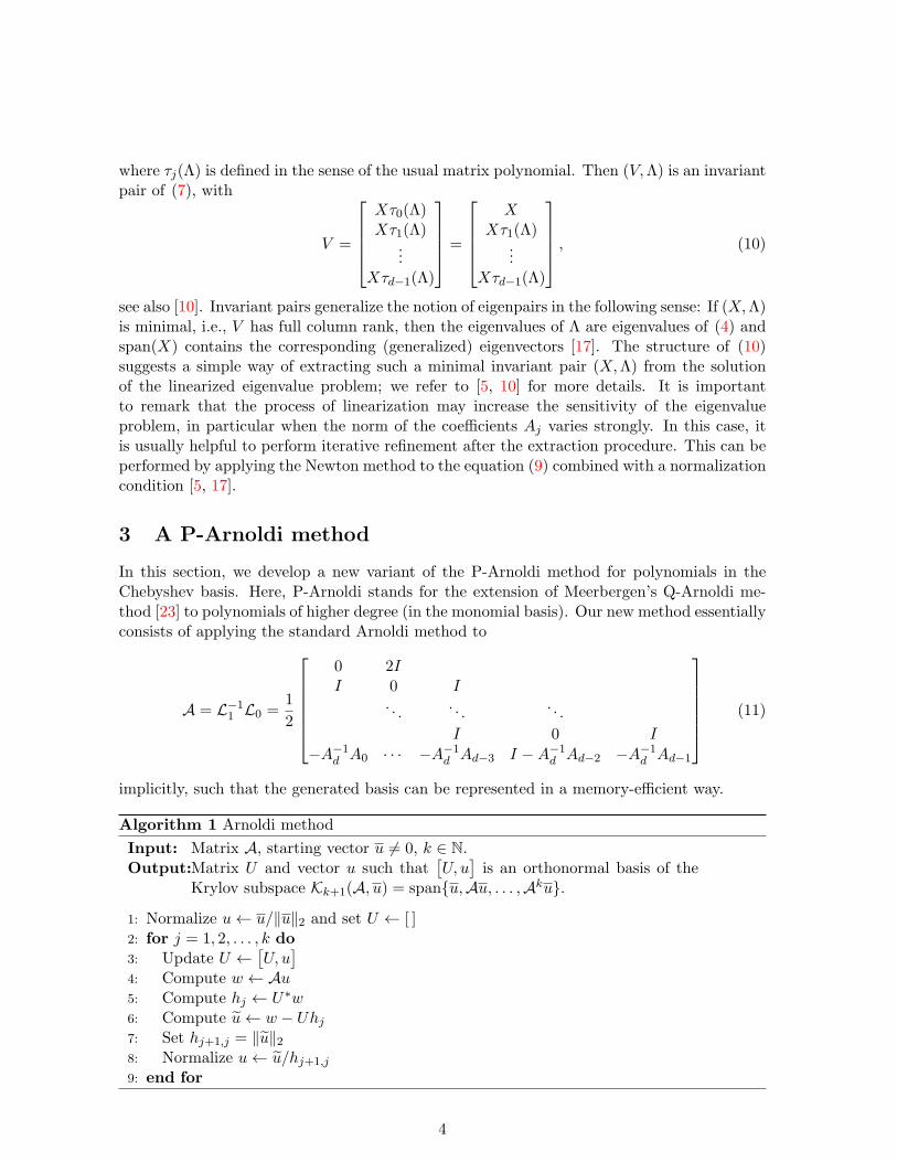
Algorithm 1 shows the standard Arnoldi method, which produces the so called Arnoldirelation
AU = UH + βue∗k, (12)
where H is a Hessenberg matrix collecting the vectors hj and scalars hj+1,j generated duringthe algorithm. Moreover, β = hk+1,k, and ek is the kth unit vector of length k. It willsometimes be convenient to express the Arnoldi decomposition (12) as
AU =[U, u
]H, (13)
where H =
[Hβe∗k
].
For simplicity, the description of Algorithm 1 omits some important implementationdetails, such as reorthogonalization. We refer, e.g., to the ARPACK users’ guide [18] orSLEPc [14] documentation for such details.
3.1 Structure of the Krylov subspace basis
As the polynomial degree d increases, the memory consumption of Algorithm 1 grows signifi-cantly due to the need to store the dn×k basis U . In the following, we explain how this effectcan be avoided by exploiting the structure of U induced by the structure of the linearization.For this purpose, we partition
U =
U0...
Ud−1
, u =
u0...
ud−1
(14)
conformally with A. The goal of our P-Arnoldi method will be to carry out all computationswithout explicit reference to the U1, . . . , Ud−1 blocks, so that only the n× k matrix U0 needsto be stored.
A compact representation of U can be derived from the block rows of the Arnoldi de-composition (13). For example, by using the structure of A in (11) the first block row gives
U1 =[U0, u0
]H. (15)
The second block row gives1
2U0 +
1
2U2 =
[U1, u1
]H,
and hence U2 = 2[U1, u1
]H − U0. More generally, the jth row block yields
Uj = 2[Uj−1, uj−1
]H − Uj−2, j = 2, . . . , d− 1. (16)
This already shows that we can reconstruct all Uj blocks from U0, u, H, and β. The followinglemma yields a more explicit expression for (16).
Lemma 1. Given an Arnoldi decomposition (13), with U and u partitioned as in (14), therelation
Uj = UjBj (17)
5
holds for all j = 1, . . . , d−1, where Uj =[U0, u0, . . . , uj−1
], and Bj is defined by the recurrence
B0 = Ik, B1 = H, Bj = 2
[Bj−1 00 1
]H −
Bj−2
00
. (18)
Proof. The proof proceeds by induction with respect to j. The case j = 0 trivially holds andthe case j = 1 follows directly from (15). For the induction step, we assume that relation (17)holds for j − 1 and j. Then the (j + 1)th block row of (13) gives
Uj+1 = 2[Uj , uj
]H − Uj−1 = 2
[UjBj , uj
]H − Uj−1
= 2[[Uj−1, uj−1
]Bj , uj
]H − Uj−1
= 2[Uj−1, uj−1, uj
] [ Bj 00 1
]H − Uj−1Bj−1
=[Uj−1, uj−1, uj
]2
[Bj 00 1
]H −
Bj−1
00
= Uj+1Bj+1.
This shows relation (17) for j + 1, which concludes the proof.
Considering Algorithm 1, the operations that need to be performed with Uj are matrix-vector products with Uj itself or with U∗
j . Lemma 1 implies that these matrix-vector productscan be performed without storing or constructing U1, . . . , Ud, once we have precomputed the(k + j) × k matrices Bj . However, this precomputation yields an additional cost of orderO(dk3), which can actually be avoided. This will be a consequence of the following result.
Lemma 2. Given an Arnoldi decomposition (12), with U and u partitioned as in (14), therelation
Uj = U0τj(H) + βu0e∗k τj(H) + 2β
j−1∑
i=1
uie∗kτj−i(H) (19)
holds for all j = 1, . . . , d− 1, where τ0, . . . , τd−1 denote the Chebyshev polynomials of secondkind, defined by the recursion
τ0(λ) = 0, τ1(λ) = 1, τj+1(λ) = 2λτj(λ)− τj−1(λ). (20)
Proof. Again, the proof proceeds by induction with respect to j. The case j = 0 triviallyholds. For the case j = 1, consider the first block row of (12):
U1 = U0H + βu0e∗k = U0τ1(H) + βu0e
∗kτ1(H).
This coincides with (19) for j = 1. For the induction step, we assume that relation (19) holds
6

for j − 1 and j. Then the (j + 1)th block row of (13) gives
Uj+1 = 2UjH − Uj−1 + 2βuje∗k
= U0 (2τj(H)H − τj−1(H)) + βu0e∗k (τj(H)H − τj−1(H))
+4β
j−1∑
i=1
uie∗kτj−i(H)H − 2β
j−2∑
i=1
uie∗k τj−i−1(H) + 2βuje
∗k
= U0τj+1(H) + βu0e∗kτj+1(H) + 2β
j−2∑
i=1
uie∗kτj−i+1(H)
+4βuj−1e∗kH + 2βuje
∗k
= U0τj+1(H) + βu0e∗kτj+1(H) + 2β
j∑
i=1
uie∗kτj−i+1(H),
which coincides with (19) for j + 1 and thus concludes the proof.
3.2 Algorithmic details
We now proceed with discussing the efficient implementation of the three main computationaltasks required by the Arnoldi algorithm, i.e., steps 4–6 in Algorithm 1. The first task, thematrix-vector product with A, is straightforward and is shown in Algorithm 2.
Algorithm 2 P-Arnoldi: Matrix-vector product with A
Input: Matrix A, vector u partitioned as in (14)Output:Vector w = Au partitioned as u
1: Set w0 = u12: for j = 1, . . . , d− 2 do
3: Set wj =12(uj−1 + uj+1)
4: end for
5: Compute wd−1 =12ud−2 −
12A
−1d
d−1∑
i=0
Aiui
For steps 5 and 6, which perform the orthogonalization against the Arnoldi basis U , wewill make use of Lemma 2. In step 5 of Algorithm 1, the orthogonalization coefficient hj iscomputed, which amounts to evaluating an expression of the form
hj =d−1∑
j=0
U∗j wj =
d−1∑
j=0
τj(H∗)U∗
0wj + βd−1∑
j=0
u∗0wj τj(H∗)ek + 2β
d−1∑
j=0
j−1∑
i=1
u∗iwj τj−i(H∗)ek (21)
for given vectors w0, . . . , wd−1. The first sum in (21) can be evaluated by Clenshaw’s algorithm[9] for evaluating polynomials in Chebyshev basis. This requires the computation of d − 1matrix-vector products U∗
0wj , which can be reorganized as a single matrix-matrix product:U∗0 [w0, . . . , wd−1]. The last two sums in (21) amount to a matrix-matrix multiplication with
the k × (d− 1) matrix
T = β [τd−1(H∗)ek, . . . , τ2(H
∗)ek, τ1(H∗)ek] (22)
7
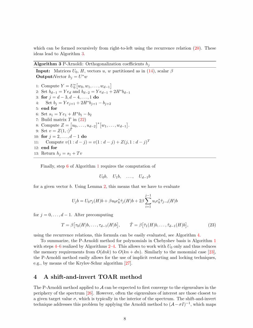
which can be formed recursively from right-to-left using the recurrence relation (20). Theseideas lead to Algorithm 3.
Algorithm 3 P-Arnoldi: Orthogonalization coefficients hj
Input: Matrices U0, H, vectors u, w partitioned as in (14), scalar βOutput:Vector hj = U∗w
1: Compute Y = U∗0
[w0, w1, . . . , wd−1
]
2: Set bd−1 = Y ed and bd−2 = Y ed−1 + 2H∗bd−1
3: for j = d− 3, d− 4, . . . , 1 do
4: Set bj = Y ej+1 + 2H∗bj+1 − bj+2
5: end for
6: Set s1 = Y e1 +H∗b1 − b27: Build matrix T in (22)8: Compute Z =
[u0, . . . , ud−2
]∗[w1, . . . , wd−1
].
9: Set v = Z(1, :)T
10: for j = 2, . . . , d− 1 do
11: Compute v(1 : d− j) = v(1 : d− j) + Z(j, 1 : d− j)T
12: end for
13: Return hj = s1 + Tv
Finally, step 6 of Algorithm 1 requires the computation of
U0b, U1b, . . . , Ud−1b
for a given vector b. Using Lemma 2, this means that we have to evaluate
Ujb = U0τj(H)b+ βu0e∗k τj(H)b+ 2β
j−1∑
i=1
uie∗kτj−i(H)b
for j = 0, . . . , d− 1. After precomputing
T = β[τ0(H)b, . . . , τd−1(H)b
], T = β
[τ1(H)b, . . . , τd−1(H)b
], (23)
using the recurrence relations, this formula can be easily evaluated, see Algorithm 4.To summarize, the P-Arnoldi method for polynomials in Chebyshev basis is Algorithm 1
with steps 4–6 realized by Algorithms 2–4. This allows to work with U0 only and thus reducesthe memory requirements from O(dnk) to O(kn+ dn). Similarly to the monomial case [23],the P-Arnoldi method easily allows for the use of implicit restarting and locking techniques,e.g., by means of the Krylov-Schur algorithm [27].
4 A shift-and-invert TOAR method
The P-Arnoldi method applied to A can be expected to first converge to the eigenvalues in theperiphery of the spectrum [26]. However, often the eigenvalues of interest are those closest toa given target value σ, which is typically in the interior of the spectrum. The shift-and-inverttechnique addresses this problem by applying the Arnoldi method to (A−σI)−1, which maps
8

Algorithm 4 P-Arnoldi: Matrix-vector product Ub
Input: Matrices U0 = [u1, . . . , uk], H, vector u partitioned as in (14), vector b, scalarβ
Output:Ub
1: Build matrices T and T in (23)2: Compute [v1, . . . , vd−1] := eTk T3: Set
C =
v1 v2 v3 · · · vd−1
2v1 2v2 · · · 2vd−2
2v1. . .
.... . . 2v2
2v1
4: Return vec(U0T + [u0, . . . , ud−2]C)
the eigenvalues closest to σ to largest magnitude eigenvalues. In this section, we focus on theparticular case σ = 0 and comment on the case σ 6= 0 in Section 4.3.
After k steps of the Arnoldi method applied to A−1 we obtain a relation of the form
A−1U = UH + βue∗k. (24)
Multiplying with A and H−1 from both sides to (24) yields
AU = UH−1 + βue∗ (25)
with u = −Au and e = H−∗ek. This has (nearly) the same form as (12) and an obviousextension of Lemma 2 can be applied. Hence, the relation (25) makes it possible to extendthe P-Arnoldi to this situation. Note that the extraction of Ritz pairs is performed in thestandard way, i.e., based on (24). When performing experiments with the resulting P-Arnoldimethod for A−1, we encountered numerical difficulties for larger d. These difficulties are dueto the fact that the norms of τj(H
−1) grow quickly if H−1 has eigenvalues too far away fromthe interval [−1, 1]. Although in applications involving larger d one is normally only interestedin eigenvalues on or close to that interval, this does not prevent some Ritz values from beingfar away from [−1, 1]. To some extent, these problems can be addressed by using a restartingstrategy that purges all such Ritz values. However, it turns out that there is a more elegantsolution, which will be discussed in this section.
4.1 Two-level orthogonalization Arnoldi (TOAR)
The instability of the P-Arnoldi method is due to the presence of τj(H−1) in the representation
of the orthonormal Arnoldi basis U . In the following, we will extend the TOAR method [20],which avoids the use of such polynomials and thus preserves stability, to polynomials inChebyshev basis. More specifically, TOAR uses the representation
[U, u] =
QV0 Qv0...
...QVd−1 Qvd−1
=
Q. . .
Q
[V v
], (26)
9

with Q ∈ Cn×(d+k), Q∗Q = I, and V ∈ C
d(d+k)×k, [V, v]∗[V, v] = I. Note that it may happenthat the number of columns of Q becomes less than d+ k in the course of the method , dueto the removal of linearly dependent vectors. For simplicity, we neglect this possibility in thefollowing description and refer to [20] for details.
Similar to the previous section, we will now discuss the efficient implementation of steps 4–6 of the Arnoldi method (Algorithm 1) applied to A−1, and the expansion of the basis repre-sentation (26).
Matrix-vector product. To compute w = A−1u with u represented as in (26), we haveto solve the linear system
w0
w1...
wd−2
wd−1
=
0 II 0 I
. . .. . .
. . .
I 0 I−A0 · · · −Ad−3 Ad −Ad−2 −Ad−1
−1
Qv02Qv1...
2Qvd−2
2AdQvd−1
.
This can be solved with the recurrences described in [10, §2.3]. For odd indices, the recurrencetakes the form
w1 = Qv0, w2j+1 = 2Qv2j − w2j−1, j = 1, 2, . . . , (27a)
while for even indicesw2j = y2j−1 + (−1)jw0, j = 1, 2, . . . , (27b)
wherey1 = 2Qv1, y2j+1 = 2Qv2j+1 − y2j−1, j = 1, 2, . . . , (27c)
and w0 is obtained from solving the linear system
(−A0 +A2 −A4 +A6 − · · · )w0 = (A1w1 +A3w3 +A5w5 + · · · )
+(A2y1 +A4y3 +A6y5 + · · · ).
For this purpose the LU decomposition of M = (−A0 +A2 −A4 +A6 − · · · ) is precomputedonce and for all. As we will see below, only the first block w0 is needed in the subsequent stepsof the Arnoldi method. This results in a (minor) computational saving, see Algorithm 5. Onthe other hand, there is some overhead involved with reconstructing the vector u from Q andv. Fortunately, this computation can be arranged in a way such that a single matrix-matrixmultiplication is sufficient, see step 5 of Algorithm 5.
Computation of U∗w. The first step of the orthogonalization procedure consists of com-puting U∗w = V ∗(I ⊗ Q)∗w, where ⊗ denotes the usual Kronecker product. Taking intoaccount the presence of Q in the recurrences (27), the following lemma derives analogousrecurrences for the components of w = (I ⊗Q)∗w.
Lemma 3. For given v0, . . . , vd−1 and w0 = Q∗w0 ∈ Ck, let the vectors wi, i = 1, . . . , d − 1
be defined by the recurrences
w1 = v0, w2j+1 = 2v2j − w2j−1, j = 1, 2, . . . , (28a)
w2j = y2j−1 + (−1)jw0, j = 1, 2, . . . , (28b)
y1 = 2v1, y2j+1 = 2v2j+1 − y2j−1, j = 1, 2, . . . . (28c)
10
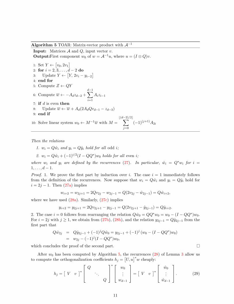
Algorithm 5 TOAR: Matrix-vector product with A−1
Input: Matrices A and Q, input vector v.Output:First component w0 of w = A−1u, where u = (I ⊗Q)v.
1: Set Y ←[v0, 2v1
]
2: for i = 2, 3, . . . , d− 2 do
3: Update Y ←[Y, 2vi − yi−2
]
4: end for
5: Compute Z ← QY
6: Compute w ← −Adzd−2 +d−1∑
i=1
Aizi−1
7: if d is even then
8: Update w ← w +Ad(2AdQvd−1 − zd−3)9: end if
10: Solve linear system w0 ←M−1w with M =
⌊(d−2)/2⌋∑
j=0
(−1)(j+1)A2i
Then the relations
1. wi = Qwi and yi = Qyi hold for all odd i;
2. wi = Qwi + (−1)i/2(I −QQ∗)w0 holds for all even i;
where wi and yi are defined by the recurrences (27). In particular, wi = Q∗wi for i =1, . . . , d− 1.
Proof. 1. We prove the first part by induction over i. The case i = 1 immediately followsfrom the definition of the recurrences. Now suppose that wi = Qwi and yi = Qyi hold fori = 2j − 1. Then (27a) implies
wi+2 = w2j+1 = 2Qv2j − w2j−1 = Q(2v2j − w2j−1) = Qwi+2,
where we have used (28a). Similarly, (27c) implies
yi+2 = y2j+1 = 2Qv2j+1 − y2j−1 = Q(2v2j+1 − y2j−1) = Qyi+2.
2. The case i = 0 follows from rearranging the relation Qw0 = QQ∗w0 = w0 − (I −QQ∗)w0.For i = 2j with j ≥ 1, we obtain from (27b), (28b), and the relation y2j−1 = Qy2j−1 from thefirst part that
Qw2j = Qy2j−1 + (−1)jQw0 = y2j−1 + (−1)j (w0 − (I −QQ∗)w0)
= w2j − (−1)j(I −QQ∗)w0,
which concludes the proof of the second part.
After w0 has been computed by Algorithm 5, the recurrences (28) of Lemma 3 allow usto compute the orthogonalization coefficients hj =
[U, u
]∗w cheaply:
hj =[V v
]∗
Q. . .
Q
∗
w0...
wd−1
=
[V v
]∗
w0...
wd−1
. (29)
11
Expansion of basis. From the discussion above, it is already clear that the vector w0
carries all the information needed for expanding the basis. The following theorem formalizesthis statement.
Theorem 4. Suppose that[U, u
]satisfies the Arnoldi decomposition (24) and is partitioned
as in (14). Moreover, let Q be an orthonormal basis of span{U0, u0, U1, u1, . . . , Ud−1, ud−1
}.
Consider the vector u that is obtained from orthogonalizing w = A−1u against span{U, u
}.
Thenspan
{U0, u0, u0, U1, u1, u1, . . . , Ud−1, ud−1, ud−1
}= span{Q,w0},
where w0 is the first block of w.
Proof. Inspecting the recursions (27), the vectors w1, . . . , wd−1 are obtained as linear combi-nations of w0 and vectors from span{Q}. We therefore have
span{U0, u0, w0, U1, u1, w1, . . . , Ud−1, ud−1, wd−1
}= span{Q,w0},
which completes the proof because replacing w by u = w −[U, u
][U, u
]∗w does not change
the space on the left.
According to Theorem 4, we expand Q with a new vector q computed as αq = w0−Qw0,where w0 = Q∗w0 and α = ‖w0 − Qw0‖2. The next step in the Arnoldi process consists ofcompleting the orthogonalization of w:
u = w − [U, u]hj =
w0...
wd−1
−
Q. . .
Q
[V v
]hj . (30)
For this purpose, we first compute the vector s resulting from Gram-Schmidt orthogonaliza-tion of w = (I ⊗Q)∗w against [V, v]:
s0...
sd−1
=
w0...
wd−1
−
[V v
]hj . (31)
Using the relations of Lemma 3, the blocks of (30) with odd index satisfy
u2j+1 = w2j+1 −Q(w2j+1 − s2j+1) = Qs2j+1,
while the blocks with even index satisfy
u2j = w2j −Q(w2j − s2j) = Qs2j + (−1)j(I −QQ∗)w0 =[Q q
] [ s2j(−1)jα
].
Therefore, the orthogonal matrix [V, v] is expanded with the vector
v =[s∗0, α, s
∗1, 0, s
∗2,−α, s
∗3, 0, . . .
]∗
after normalization. Note that ‖v‖2 = ‖u‖2 =: hj+1,j .
12

Algorithm 6 Two-level orthogonalization Arnoldi (TOAR) method for A−1
Input: Matrix A, starting vector u 6= 0, k ∈ N
Output:Matrices Q,[V, v
]such that the matrix
[U, u
]defined in (26) is an or-
thonormal basis of Kk+1(A−1, u)
1: Normalize u← u/‖u‖22: Compute QR factorization
[u0, u1, . . . , ud−1
]= QR with R = [r0, . . . , rd−1] ∈ R
d×d
3: Set V ← [ ] and v ←[r∗0, r
∗1, . . . , r
∗d−1
]∗4: for j = 1, 2, . . . , k do
5: Compute w0 using Algorithm 56: Compute w0 ← Q∗w0 and q ← w0 −Qx07: Normalize α← ‖q‖2, q ← q/α8: Update Q←
[Q, q
]
9: Compute wi for i = 1, . . . , d−1 using the recurrences (28) and set w ←[w∗0, . . . , w
∗d−1
]∗
10: Compute hj ←[V, v
]∗w and s← w −
[V, v
]hj
11: Update components of V : V0 ←[V0 v00 0
], V1 ←
[V1 v10 0
], . . ., Vd−1 ←
[Vd−1 vd−1
0 0
]
12: Set v =[s∗0, α, s
∗1, 0, s
∗2,−α, s
∗3, 0, . . .
]∗13: Normalize v ← v/hj+1,j with hj+1,j = ‖v‖214: end for
Summary. The considerations above lead to the TOAR method for A−1 summarized inAlgorithm 6. The first and second level orthogonalizations are carried out in line 6 and 10,respectively. In both cases, reorthogonalization can (and should) be done if required. Apartfrom the memory savings, Algorithm 6 also entails a significant increase of computationalefficiency compared to standard Arnoldi or P-Arnoldi for larger d. This is due to fact thatorthogonalization is much cheaper, with the main cost being concentrated in the first level,which involves only the matrix Q. Although the second level orthogonalization causes someoverhead, its cost remains negligible for n≫ k.
4.2 Krylov-Schur Restart
In practical implementations of Arnoldi methods, it is fundamental to incorporate an effectiverestarting strategy. In the following, we will propose such a strategy for TOAR based on theKrylov-Schur method, by adapting and extending the discussion on implicit restarting TOARfor the monomial representation in [28].
The Krylov-Schur method [27] is based on generalizing the Arnoldi decomposition (24) toa Krylov decomposition
A−1U = UB + ub∗, (32)
where B is a general k × k matrix (not necessarily in Hessenberg form) and b is a generalvector of length k.
To restart the Krylov decomposition (32), we first compute the Schur form B = Y SY ∗
with an upper triangular matrix S and a unitary matrix Y . Applying this transformationto (32) yields
A−1U = US + ub∗, (33)
13

where U = UY and b = Y ∗b. The ordering of the eigenvalues in the Schur form S is suchthat the p < k Ritz values of interest are contained in its leading principal p × p submatrixS. We then truncate (33) to
A−1U = U S + ub∗, (34)
with U = UY , where Y contains the first p columns of Y and b contains the first p entriesof b. The Arnoldi process is continued from (34) by expanding the decomposition again toorder k, truncating it back to order p, and so on.
Let us now consider the case that the decomposition (32) has been generated with Al-gorithm 6, yielding the representation (26) of
[U, u
]. Then the components of U satisfy
Uj = QVj with orthonormal Q ∈ Cn×(d+k) and Vj ∈ C
(d+k)×k. In principle, the restartingprocedure described above can be implemented in a straightforward fashion, by simply keep-ing only the first p columns of VjY . However, this would not effect the desired reduction asthe (usually much larger) factor Q remains of the same size.
In order to also truncateQ, let us recall that Theorem 4 implies that[U0, u0, U1, u1, . . . , Ud−1, ud−1
]
and consequently also[V0, v0, V1, v1, . . . , Vd−1, vd−1
]have rank d+k only. Similarly, the matrix
[V0Y , v0, V1Y , v1, . . . , Vd−1Y , vd−1
](35)
has rank d+ p. This is due to its relation to the truncated Krylov-Schur decomposition (34),which can be retransformed into a standard Arnoldi decomposition [27] of order p (withdifferent starting vector) and hence Theorem 4 applies. By, e.g., a truncated SVD, we canfind an orthonormal matrix W ∈ C
(d+k)×(d+p) such that its columns span the row space ofthe matrix in (35). If we now define
Q = QW, Vj = W ∗Vj Y , vj = W ∗vj , j = 0, . . . , d− 1,
then we obtain the following representation of the truncated Arnoldi basis U :
[U , u] =
QV0 Qv0...
...
QVd−1 Qvd−1
.
This is exactly the form of the usual representation (26) in the TOAR method, allowing usto expand the truncated Arnoldi decomposition (34) using the techniques of Algorithm 6.
4.3 Extension to σ 6= 0
In this section, we briefly discuss the extension of the TOAR method described above to σ 6= 0,that is, the shift-and-invert Arnoldi method operating with (L0 − σL1)
−1L1 for a nonzeroshift σ. For this purpose, it is useful to note that the recurrences (27), which provided thefoundation of TOAR, can be derived from a block LU factorization of the matrix L0.
In the following, we derive a generalization of the recurrences (27) from a block LUfactorization of the matrix
L0 − σL1 =
−σI II −2σI I
I −2σI I. . .
. . .. . .
I −2σI I−A0 −A1 · · · −Ad−3 Ad −Ad−2 −Ad−1 − 2σAd
. (36)
14

For this purpose, we proceed in a way analogous to the proof of [2, Theorem 3.1]. We firstpermute the block columns as follows:
(L0 − σL1)Π =
I −σI−2σI I II −2σI I
. . .. . .
. . .
I −2σI I−A1 · · · −Ad−3 Ad −Ad−2 −Ad−1 − 2σAd −A0
,
with the block cyclic shift Π =[
0 InI(d−1)n 0
]. This matrix has the block LU factorization LσUσ
with
Lσ =
I−2σI II −2σI I
. . .. . .
. . .
I −2σI I−A1 · · · −Ad−3 Ad −Ad−2 −Ad−1 − 2σAd P (σ)
and
Uσ =
I −τ1(σ)II −τ2(σ)I
I −τ3(σ)I. . .
...I −τd−1(σ)I
I
.
Hence,(L0 − σL1)
−1 = ΠU−1σ L−1
σ . (37)
Note that U−1σ is identical with Uσ, except for a sign change in the first d − 1 blocks of the
last block column.Using (37) and the block structure of Lσ, Uσ, we will now discuss the computation of w =
(L0−σL1)−1L1u for a vector u =
[u∗0, u
∗1, · · · , u
∗d−1
]∗. First, the components y0, y1, . . . , yd−1 ∈
Cn of
y := L−1σ L1u
are given by
y0 = u0
y1 = 2u1 + 2σy0
y2 = 2u2 + 2σy1 − y0...
yd−2 = 2ud−2 + 2σyd−3 − yd−4
yd−1 = w0,
with
w0 := P (σ)−1 [2Adud−1 +A1y0 + · · ·+Ad−3yd−4 + (Ad−2 −Ad)yd−3 + (Ad−1 + 2σAd)yd−2] .
15

Using thatw = ΠU−1
σ y,
this yields the following expressions for its components w0, w1, . . . , wd−1 ∈ Rn:
w0 = w0
w1 = u0 + τ1(σ)w0
w2 = 2u1 + 2σy0 + τ2(σ)w0
w3 = 2u2 + 2σy1 − y0 + τ3(σ)w0
...
wd−1 = 2ud−2 + 2σyd−3 − yd−4 + τd−1(σ)w0.
These formulas can be used in place of the recurrences (27) to develop a TOAR method fornonzero σ. In particular, when applying (L0−σL1)
−1L1 to a vector u represented as in (26),it is possible to pull out the matrix Q and derive recurrences for the reduced vectors analogousto (28), Apart from these changes, there is only one additional modification required to adaptAlgorithm 6: the vector v generated in step 12 of Algorithm 6 to expand V now takes theform
v =
s0τ0(σ)αs1
τ1(σ)α...
sd−1
τd−1(σ)α
. (38)
Remark 5. The linearizations discussed in [2] for general polynomial bases satisfying a three-term recurrence relation all admit a highly structured block LU factorization similar to theone discussed above. It is therefore likely that the TOAR method can be extended to this moregeneral setting. However, we feel that a detailed discussion would go beyond the scope of thispaper.
5 Numerical experiments
We have evaluated the performance of the shift-and-invert TOAR method from Section 4 onthree application problems. Our examples arise from certain discretizations of elliptic PDEeigenvalue problems, leading to a nonlinear eigenvalue problem
T (λ)x = 0, x 6= 0, (39)
where T : C → Cn×n is an analytic matrix-valued function. The solution of this problem
can be approximated by replacing T (λ) with a polynomial P (λ) interpolating T at d + 1interpolation points. In particular, when the eigenvalues on or very close to a real intervalare of interest, interpolation in the Chebyshev points can be used. As discussed in [10], theresulting polynomial P of degree d can be easily represented in the Chebyshev basis. Afterevaluating T (λ) for d+ 1 values of λ, the rest of the computation proceeds with P (λ). This
16
gives an advantage, compared to solvers directly addressing (39), when the evaluation of T (λ)is very costly.
The TOAR method applied to the linearization of P results in an approximate invariantpair (V,Λ), where V has the form (10). As discussed in Section 2, we can then extract anapproximate invariant pair (X,Λ) for P . Subsequently, we apply 1 or 2 iterations of Newton’smethod to refine (X,Λ). In all our experiments below, this is sufficient to attain an accuracyon the level of machine precision.
All computations have been carried out under Matlab R2012a on a computer with anIntel Core i7 processor at 2.6 GHz with 8 GB of memory.
5.1 Laplace eigenvalue problem on the Fichera corner
We first address the 3D Laplace eigenvalue problem with Dirichlet boundary conditions [25]
−∆u = λ2u in D ⊂ R3,
u = 0 on B := ∂D,
which can be reformulated by means of the representation formula for the Helmholtz operatoras the boundary integral equation
1
4π
∫
B
eiλ‖ξ−η‖
‖ξ − η‖un(η)dS(η) = 0 for all ξ ∈ B,
where un is the exterior normal derivative of u. A Galerkin-based discretization eventuallyleads to a nonlinear eigenvalue problem (39). We report results for the Fichera corner D =[0, 1]3\[12 , 1]
3 using a boundary element space of piecewise constant functions on a surfacemesh of 2400 triangles (h = 0.1).
We have run the method of section 4 for various degrees d of the interpolating Chebyshevpolynomial, from d = 3 up to d = 30, and compared it with applying the standard Krylov-Schur algorithm. The solvers were configured to compute 6 eigenvalues with a maximumsubspace dimension of k = 24 and a convergence tolerance 10−12 for the norm of the residual.The reported results are averaged over 20 runs with random initial vectors.
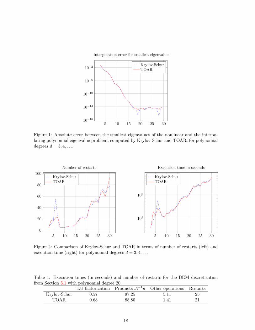
Figure 1 confirms the spectral convergence of the smallest computed eigenvalue as theinterpolation degree increases. As expected, both TOAR and Krylov-Schur behave similarly,and full machine precision is achieved already for a polynomial of degree 17.
TOAR and Krylov-Schur behave very similarly in terms of the number of required restartsand execution time, see Figure 2. The latter is due to the fact that the computational costis dominated by operations involving the coefficients Ai of the polynomial. Our currentimplementation does not make use of fast techniques for boundary element discretizations,like hierarchical matrices, and treats Ai as dense matrices. We expect that incorporatingsuch a fast technique significantly decreases the time spent on operations with Ai. This likelyresults in a more pronounced difference between the execution times for TOAR and Krylov-Schur. This can be seen from Table 1, where we have accounted for the times spent on theinitial LU factorization of P (0), on the matrix-vector products w = A−1u and on all otheroperations separately. It turns out that Krylov-Schur takes 0.20 seconds per restart, whereasTOAR takes only 0.07 seconds, when neglecting the times for the LU factorization and thematrix-vector products. However, we would like to emphasize that the major computationalsaving is in the additional memory required for storing the basis vectors; this is reduced by afactor of approximately d when using TOAR.
17
5 10 15 20 25 3010−18
10−14
10−10
10−6
10−2
Interpolation error for smallest eigenvalue
Krylov-SchurTOAR
Figure 1: Absolute error between the smallest eigenvalues of the nonlinear and the interpo-lating polynomial eigenvalue problem, computed by Krylov-Schur and TOAR, for polynomialdegrees d = 3, 4, . . ..
5 10 15 20 25 30
0
20
40
60
80
100
Number of restarts
Krylov-SchurTOAR
5 10 15 20 25 30
101
102
Execution time in seconds
Krylov-SchurTOAR
Figure 2: Comparison of Krylov-Schur and TOAR in terms of number of restarts (left) andexecution time (right) for polynomial degrees d = 3, 4 . . ..
Table 1: Execution times (in seconds) and number of restarts for the BEM discretizationfrom Section 5.1 with polynomial degree 20.
LU factorization Products A−1u Other operations Restarts
Krylov-Schur 0.57 97.25 5.11 25TOAR 0.68 88.80 1.41 21
18
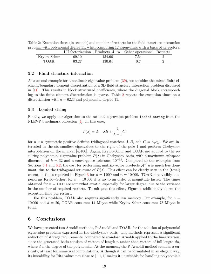
Table 2: Execution times (in seconds) and number of restarts for the fluid-structure interactionproblem with polynomial degree 11, when computing 12 eigenvalues with a basis of 48 vectors.
LU factorization Products A−1u Other operations Restarts
Krylov-Schur 69.10 134.66 7.54 2TOAR 63.27 130.64 0.7 2
5.2 Fluid-structure interaction
As a second example for a nonlinear eigenvalue problem (39), we consider the mixed finite el-ement/boundary element discretization of a 3D fluid-structure interaction problem discussedin [11]. This results in block structured coefficients, where the diagonal block correspond-ing to the finite element discretization is sparse. Table 2 reports the execution times on adiscretization with n = 6223 and polynomial degree 11.
5.3 Loaded string
Finally, we apply our algorithm to the rational eigenvalue problem loaded string from theNLEVP benchmark collection [4]. In this case,
T (λ) = A− λB +λ
λ− 1C
for n × n symmetric positive definite tridiagonal matrices A,B, and C = eneTn . We are in-
terested in the six smallest eigenvalues to the right of the pole 1 and perform Chebyshevinterpolation on the interval [4, 400]. Again, Krylov-Schur and TOAR are applied to the re-sulting polynomial eigenvalue problem P (λ) in Chebyshev basis, with a maximum subspacedimension of k = 32 and a convergence tolerance 10−12. Compared to the examples fromSections 5.1 and 5.2, the cost for performing matrix-vector products A−1u is much less dom-inant, due to the tridiagonal structure of P (λ). This effect can be clearly seen in the (total)execution times reported in Figure 3 for n = 1000 and n = 10 000. TOAR now visibly out-performs Krylov-Schur; for n = 10 000 it is up to an order of magnitude faster. The timesobtained for n = 1000 are somewhat erratic, especially for larger degree, due to the variancein the number of required restarts. To mitigate this effect, Figure 4 additionally shows theexecution time per restart.
For this problem, TOAR also requires significantly less memory. For example, for n =10 000 and d = 20, TOAR consumes 14 Mbyte while Krylov-Schur consumes 73 Mbyte intotal.
6 Conclusions
We have presented two Arnoldi methods, P-Arnoldi and TOAR, for the solution of polynomialeigenvalue problems expressed in the Chebyshev basis. The methods represent a significantreduction of storage requirements, compared to standard Arnoldi applied to the linearization,since the generated basis consists of vectors of length n rather than vectors of full length dn,where d is the degree of the polynomial. At the moment, the P-Arnoldi method remains a cu-riosity, at least for numerical computations. Although it can be formulated in an elegant way,its instability for Ritz values not close to [−1, 1] makes it unsuitable for handling polynomials
19

5 10 15 20 2510−2
10−1
100
101
102
Execution time in seconds
Krylov-SchurTOAR
5 10 15 20 25
10−1
100
101
102
103
Execution time in seconds
Krylov-SchurTOAR
Figure 3: Comparison of execution time of Krylov-Schur and TOAR when solving the loadedstring problem for n = 1000 (left) and n = 10 000 (right) for polynomial degrees d = 3, 4 . . ..
5 10 15 20 25
10−1.6
10−1.4
10−1.2
10−1
Execution time in seconds
Krylov-SchurTOAR
5 10 15 20 2510−1
100
Execution time in seconds
Krylov-SchurTOAR
Figure 4: Comparison of execution time per restart of Krylov-Schur and TOAR when solvingthe loaded string problem for N = 1000 (left) and N = 10 000 (right) for polynomial degreesd = 3, 4 . . ..
20
of larger degree. In contrast, the TOAR method appears to be numerically stable even forcomparably large degrees. Moreover, we have shown that it is possible to turn this into a fullyfledged Arnoldi algorithm, by incorporating shift-and-invert and restarting techniques. Allthese ingredients are crucial for addressing polynomial eigenvalue problems that arise fromthe interpolation of discretized nonlinear PDE eigenvalue problems. Our numerical experi-ments demonstrate the advantages of our algorithm compared to the standard approach interms of memory requirements and computational time.
As indicated in Remark 5, there is nothing particular about the Chebyshev basis; allalgorithms can certainly be extended to more general polynomial bases satisfying a three-term recurrence. Another possible extension would consist of using the Krylov subspacemethods developed in this paper for solving linear systems with P (λ) for many differentvalues of λ [13].
Acknowledgments
The authors thank Cedric Effenberger for many insightful discussions and for providing thematrices used in the numerical experiments. They also thank Yangfeng Su for sending apreprint of [20]. This work was carried out while the second author was visiting EPFL duringthe Spring 2013.
References
[1] B. Adhikari, R. Alam, and D. Kressner. Structured eigenvalue condition numbers andlinearizations for matrix polynomials. Linear Algebra Appl., 435(9):2193–2221, 2011.
[2] A. Amiraslani, R. M. Corless, and P. Lancaster. Linearization of matrix polynomialsexpressed in polynomial bases. IMA J. Numer. Anal., 29(1):141–157, 2009.
[3] Z. Bai and Y. Su. SOAR: a second-order Arnoldi method for the solution of the quadraticeigenvalue problem. SIAM J. Matrix Anal. Appl., 26(3):640–659, 2005.
[4] T. Betcke, N. J. Higham, V. Mehrmann, C. Schroder, and F. Tisseur. NLEVP: Acollection of nonlinear eigenvalue problems. MIMS EPrint 2011.116, Manchester Institutefor Mathematical Sciences, The University of Manchester, UK, December 2011.
[5] T. Betcke and D. Kressner. Perturbation, extraction and refinement of invariant pairsfor matrix polynomials. Linear Algebra Appl., 435(3):574–536, 2011.
[6] W.-J. Beyn and V. Thummler. Continuation of invariant subspaces for parameterizedquadratic eigenvalue problems. SIAM J. Matrix Anal. Appl., 31(3):1361–1381, 2009.
[7] D. Bindel and A. Hood. Localization theorems for nonlinear eigenvalues. arXiv:1303.4668,2013.
[8] M. A. Botchev, G. L. G. Sleijpen, and A. Sopaheluwakan. An SVD-approach to Jacobi-Davidson solution of nonlinear Helmholtz eigenvalue problems. Linear Algebra Appl.,431(3-4):427–440, 2009.
21
[9] C. W. Clenshaw. A note on the summation of Chebyshev series. Mathematics of Com-putation, 9(51):118–120, 1955.
[10] C. Effenberger and D. Kressner. Chebyshev interpolation for nonlinear eigenvalue prob-lems. BIT, 52(4):933–951, 2012.
[11] C. Effenberger, D. Kressner, O. Steinbach, and G. Unger. Interpolation-based solutionof a nonlinear eigenvalue problem in fluid-structure interaction. PAMM, 12(1):633–634,2012.
[12] G. H. Golub and C. F. Van Loan. Matrix Computations. Johns Hopkins UniversityPress, Baltimore, MD, third edition, 1996.
[13] L. Grammont, N. J. Higham, and F. Tisseur. A framework for analyzing nonlineareigenproblems and parametrized linear systems. Linear Algebra Appl., 435(3):623–640,2011.
[14] V. Hernandez, J. E. Roman, and V. Vidal. SLEPc: a scalable and flexible toolkit for thesolution of eigenvalue problems. ACM Trans. Math. Software, 31(3):351–362, 2005.
[15] N. J. Higham, D. S. Mackey, and F. Tisseur. The conditioning of linearizations of matrixpolynomials. SIAM J. Matrix Anal. Appl., 28(4):1005–1028, 2006.
[16] N. Kamiya, E. Andoh, and K. Nogae. Eigenvalue analysis by the boundary elementmethod: new developments. Engng. Anal. Bound. Elms., 12:151–162, 1993.
[17] D. Kressner. A block Newton method for nonlinear eigenvalue problems. Numer. Math.,114(2):355–372, 2009.
[18] R. B. Lehoucq, D. C. Sorensen, and C. Yang. ARPACK users’ guide. SIAM, Philadelphia,PA, 1998. Solution of large-scale eigenvalue problems with implicitly restarted Arnoldimethods.
[19] Y. Lin, L. Bao, and Y. Wei. Model-order reduction of large-scale kth-order linear dynam-ical systems via a kth-order Arnoldi method. Int. J. Comput. Math., 87(1-3):435–453,2010.
[20] Y. Lu and Y. Su. Two-level orthogonal Arnoldi process for the solution of quadraticeigenvalue problems. Submitted.
[21] D. S. Mackey, N. Mackey, C. Mehl, and V. Mehrmann. Structured polynomial eigen-value problems: good vibrations from good linearizations. SIAM J. Matrix Anal. Appl.,28(4):1029–1051, 2006.
[22] D. S. Mackey, N. Mackey, C. Mehl, and V. Mehrmann. Vector spaces of linearizationsfor matrix polynomials. SIAM J. Matrix Anal. Appl., 28(4):971–1004, 2006.
[23] K. Meerbergen. The quadratic Arnoldi method for the solution of the quadratic eigen-value problem. SIAM J. Matrix Anal. Appl., 30(4):1463–1482, 2008/09.
[24] G. A. Sitton, C. S. Burrus, J. W. Fox, and S. Treitel. Factoring very-high-degree poly-nomials. IEEE Signal Processing Magazine, 20(6):27–42, 2003.
22

[25] O. Steinbach and G. Unger. A boundary element method for the Dirichlet eigenvalueproblem of the Laplace operator. Numer. Math., 113(2):281–298, 2009.
[26] G. W. Stewart. Matrix Algorithms. Vol. II. SIAM, Philadelphia, PA, 2001. Eigensystems.
[27] G. W. Stewart. A Krylov-Schur algorithm for large eigenproblems. SIAM J. MatrixAnal. Appl., 23(3):601–614, 2001/02.
[28] Y. Su. A compact Arnoldi algorithm for polynomial eigenvalue problems, 2008. Talkpresented at RANMEP2008.
[29] L. N. Trefethen. Approximation Theory and Approximation Practice. SIAM, 2012.
[30] R. Van Beeumen, K. Meerbergen, and W. Michiels. A rational Krylov method basedon Hermite interpolation for nonlinear eigenvalue problems. SIAM J. Sci. Comput.,35(1):A327–A350, 2013.
23