arnoldi algorithm - fb3 - uni bremen || startseite · introduction applications remarks examples...

IntroductionApplications

RemarksExamples

References

Arnoldi Algorithm

NguyÔn, Thanh S¬n

Universitaet BremenZentrum fuer Technomathematik

25th March 2009

NguyÔn, Thanh S¬n Arnoldi Algorithm

RemarksExamples

References

Outline

1 Introduction

2 Applications

3 Remarks

4 Examples

5 References

RemarksExamples

References

Introduction

Arnoldi algorithm/Arnoldi process is used to produce anorthonormal basis for a Krylov subspace. Given a squarematrix A, a non-zero vector x and an integer number m,find a matrix V s.t. VTV = I and

colspan(V) = span(x,Ax,A2x, ...,Am−1x).

Invented by W. E. Arnoldi in 1951 for eigenvalue problem.

Wide-used in approximate solvers.

RemarksExamples

References

Introduction

RemarksExamples

References

Introduction

RemarksExamples

References

Introduction

RemarksExamples

References

Coding

function [V,H] = Arnoldi(A,b,m, tol)

H = zeros(m + 1,m);

beta = norm(b);

V = b/beta;

for j = 1 : m

w = AV(:, j);

for i = 1 : j

H(i, j) = w′V(:, i);

for i = 1 : j

w = w− H(i, j) ∗ V(:, i);

H(j + 1, j) = norm(w);

if H(j + 1, j) < tol

H = H(1 : j,1 : j);

V = [V w/H(j + 1, j)];

RemarksExamples

References

Coding

function [V,H] = Arnoldi(A,b,m, tol)

H = zeros(m + 1,m);

beta = norm(b);

V = b/beta;

for j = 1 : m

w = AV(:, j);

for i = 1 : j

H(i, j) = w′V(:, i);

for i = 1 : j

w = w− H(i, j) ∗ V(:, i);

H(j + 1, j) = norm(w);

if H(j + 1, j) < tol

H = H(1 : j,1 : j);

V = [V w/H(j + 1, j)];

RemarksExamples

References

Three matrices A,V,H satisfy the relations

AVm = Vm+1H(m+1)xm; (1)

VTmAVm = Hmxm. (2)

Hmxm is a Hessenberg matrix, VTmVm = Im.

This structure is useful in many situations in linear algebra.

RemarksExamples

References

Linear equations

GMRES ( Generalized Minimum RESidual method ): Givena square (usually large, sparse) system Ax = b of order N,intial guess x0, r0 = b−Ax0 called intial residual. One findsthe approximate solution in affine subspace x0 +Km(A, r0).

Let x = x0 + Vmy, y ∈ Rm, the minimization problem‖b− Ax‖2 subject to x ∈ RN is converted to minimizing‖‖r0‖e1 − H(m+1)xmy‖ subject to y ∈ Rm.

If A is nonsingular, GMRES breaks down at mth iffxm = x0 + Vmy is the exact solution.

Some other methods or variations: FOM, GCR,GMRES-DR, c.f [4, 6, 7, 8]

RemarksExamples

References

Linear equations

RemarksExamples

References

Linear equations

RemarksExamples

References

Linear equations

RemarksExamples

References

Eigenvalues problem

The original eigenvalue problem Ax = λx is replaced bythe "reduced" eigenvalue problem Hmxmzm = θzm wherethe Arnoldi basis Vm is started with a unit-normed initialeigenvector v1. Then, the approximate eigenpairs of A areselected form the Ritz pairs {(θi,Vmzm,i)}.This approach yields a better result in compare with Power

method which only uses Am−1v1 for approximation. c.f.[5]

RemarksExamples

References

Eigenvalues problem

The original eigenvalue problem Ax = λx is replaced bythe "reduced" eigenvalue problem Hmxmzm = θzm wherethe Arnoldi basis Vm is started with a unit-normed initialeigenvector v1. Then, the approximate eigenpairs of A areselected form the Ritz pairs {(θi,Vmzm,i)}.This approach yields a better result in compare with Power

method which only uses Am−1v1 for approximation. c.f.[5]

RemarksExamples

References

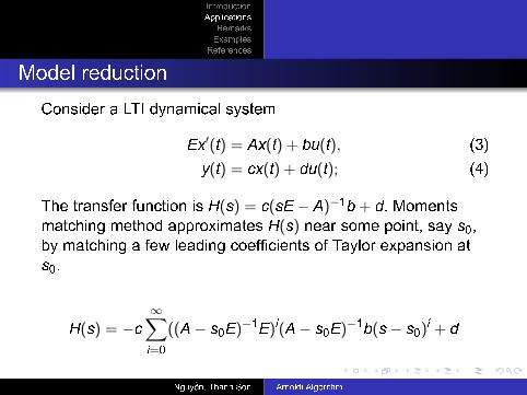
Model reduction

Consider a LTI dynamical system

Ex′(t) = Ax(t) + bu(t), (3)

y(t) = cx(t) + du(t); (4)

The transfer function is H(s) = c(sE− A)−1b + d. Momentsmatching method approximates H(s) near some point, say s0,by matching a few leading coefficients of Taylor expansion ats0.

H(s) = −c∞∑i=0

((A− s0E)−1E)i(A− s0E)−1b(s− s0)i + d

RemarksExamples

References

Model reduction

This can be done by projecting the system (3)-(4) onto Krylovsubspace V = Km((A− s0E)−1E, (A− s0E)−1b) or bothV = Km((A− s0E)−1E, (A− s0E)−1b) andW = Ki+1(((A− s0E)−1E)T,CT). The reduced systems arethen,

One-sided

VTEVx′ = VTAVx + VTbu,

y = cVx + du;

Two-sided

WTEVx′ = WTAVx + WTbu,

y = cVx + du;

RemarksExamples

References

Model reduction

One-sided

y = cVx + du;

Two-sided

y = cVx + du;

RemarksExamples

References

Model reduction

One-sided

y = cVx + du;

Two-sided

y = cVx + du;

RemarksExamples

References

Deflation may occur, if the process has not beenconvergent, restarting is required.

Restarting is also needed when the order of Krylovsubspace is big,( but under-convergent ) since thisrequires much computer memories.

Multiple starting vectors leads to so called block Arnoldi

algorithm which requires more efforts in implementation.

RemarksExamples

References

RemarksExamples

References

RemarksExamples

References

Examples

Two applications of Arnoldi algorithm in solving linearequations and model reduction are provided.

RemarksExamples

References

[Antoulas05] A. C. Antoulas, Approximation of Large-scale

Dynamical Systems, Advances in Design and ControlDC-06, SIAM, Philadenphia, 2005.

[Chahlaoui02] Y. Chahlaoui, P. V. Doreen, "A collection ofbenchmark examples for model reduction of linear timeinvariant dynamical systems", Technical report, SILICOTWorking Note 2002-2, 2002.

[Freund99] R. W. Freund, "Krylov-subspace methods forreduced-order modeling in circuit simulation", Numerical

Analysis Manuscript, No. 99-3-17, Bell Laboratories.

[Morgan02] R. B. Morgan, "GMRES with deflatedrestarting", SIAM J. Sci. Comput., Vol. 24, No. 1, pp. 20-37,2002.

RemarksExamples

References

[Saad92] Y. Saad, Numerical Methods for Eigenvalues

Problems, Manchester University Press, 1992.

[Saad96] Y. Saad, Iterative Methods for Sparse Linear

Systems, PWS Publishing Company, 1996.

[Sturler96], E. de Sturler, "Nested Krylov methods basedon GRC", J. Computational and Applied Mathematics, 67,pp. 15-41, 1996.

[Sturler99], E. de Sturler, "Truncation strategies for optimalKrylov subspace methods", SIAM J. Numer. Anal., Vol. 36,No. 3, pp. 864-889, 1999.

arnoldi algorithm - fb3 - uni bremen || startseite · introduction applications remarks examples...

Documents