mesh parameterization: theory and practice · siggraph course notes mesh parameterization: theory...

Siggraph Course Notes

Mesh Parameterization: Theory and Practice

Kai HormannClausthal University

of Technology

Bruno Lévy

INRIA

Alla ShefferThe University

of British Columbia

August 2007

Summary

Mesh parameterization is a powerful geometry processing tool with numerous computergraphics applications, from texture mapping to animation transfer. This course outlinesits mathematical foundations, describes recent methods for parameterizing meshes overvarious domains, discusses emerging tools like global parameterization and inter-surfacemapping, and demonstrates a variety of parameterization applications.

Prerequisites

The audience should have had some prior exposure to mesh representation of geometricmodels and a working knowledge of vector calculus, elementary linear algebra, and thefundamentals of computer graphics. Optional pre-requisites: some lectures may alsoassume some familiarity with differential geometry, graph theory, harmonic functions,and numerical optimization.

Intended Audience

Graduate students, researchers, and application developers who seek to understand theconcepts and technologies used in mesh parameterization and wish to utilize them. Lis-teners get an overview of the spectrum of processing applications that benefit from para-meterization and learn how to evaluate different methods in terms of specific applicationrequirements.

Sources

These notes are largely based on the following survey papers, which can be found on theauthor webpages:

• M. S. Floater and K. Hormann. Surface parameterization: a tutorial and sur-vey. In Advances in Multiresolution for Geometric Modelling, Mathematics andVisualization, pages 157–186. Springer, 2005.

• A. Sheffer, E. Praun, and K. Rose. Mesh parameterization methods and theirapplications. Foundations and Trends in Computer Graphics and Vision, 2(2):105–171, 2006.

• B. Lévy. Parameterization and deformation analysis on a manifold. Technicalreport, ALICE, 2007. http://alice.loria.fr/publications.

• Source code (Graphite, OpenNL, . . . ) can be found from http://alice.loria.fr/software.

Supplemental material and presentation slides are also available on the presenter web-pages.

i

Course Overview

For any two surfaces with similar topology, there exists a bijective mapping betweenthem. If one of these surfaces is a triangular mesh, the problem of computing sucha mapping is referred to as mesh parameterization. The surface that the mesh ismapped to is typically called the parameter domain. Parameterization was introducedto computer graphics for mapping textures onto surfaces. Over the last decade, it hasgradually become a ubiquitous tool for many mesh processing applications, includingdetail-mapping, detail-transfer, morphing, mesh-editing, mesh-completion, remeshing,compression, surface-fitting, and shape-analysis. In parallel to the increased interest inapplying parameterization, various methods were developed for different kinds of para-meter domains and parameterization properties.

The goal of this course is to familiarize the audience with the theoretical and practicalaspects of mesh parameterization. We aim to provide the skills needed to implement orimprove existing methods, to investigate new approaches, and to critically evaluate thesuitability of the techniques for a particular application.

The course starts with an introduction to the general concept of parameterizationand an overview of its applications. The first half of the course then focuses on pla-nar parameterizations while the second addresses more recent approaches for alternativedomains. The course covers the mathematical background, including intuitive expla-nations of parameterization properties like bijectivity, conformality, stretch, and area-preservation. The state-of-the-art is reviewed by explaining the main ideas of severalapproaches, summarizing their properties, and illustrating them using live demos. Thecourse addresses practical aspects of implementing mesh parameterization discussingnumerical algorithms for robustly and efficiently parameterizing large meshes and pro-viding tips on how to handle the variety of often contradicting criteria when choosing anappropriate parameterization method for a specific target application. We conclude bypresenting a list of open research problems and potential applications that can benefitfrom parameterization.

Speakers

Mathieu Desbrun, Caltech, USA

Mathieu Desbrun is an associate professor at the California Institute of Technology(Caltech) in the Computer Science department. After receiving his Ph.D. from theNational Polytechnic Institute of Grenoble (INPG), he spent two years as a post-doctoralresearcher at Caltech before starting a research group at the University of SouthernCalifornia (USC). His research interests revolve around applying discrete differentialgeometry (differential, yet readily-discretizable computational foundations) to a widerange of fields and applications such as meshing, parameterization, smoothing, fluid andsolid mechanics, etc.

ii

Kai Hormann, Clausthal University of Technology, Germany

Kai Hormann is an assistant professor for Computer Graphics in the Department ofInformatics at Clausthal University of Technology in Germany. His research interests arefocussed on the mathematical foundations of geometry processing algorithms as well astheir applications in computer graphics and related fields. Dr. Hormann has co-authoredseveral papers on parameterization methods, surface reconstruction, and barycentriccoordinates. Kai Hormann received his PhD from the University of Erlangen in 2002and spent two years as a postdoctoral research fellow at the Multi-Res Modeling Groupat Caltech, Pasadena and the CNR Institute of Information Science and Technologies inPisa, Italy.

Bruno Lévy, INRIA, France

Bruno Lévy is a Researcher with INRIA. He is the head of the ALICE INRIA Project-Team. His main contributions concern texture mapping and parameterization methodsfor triangulated surfaces, and are now used by some 3D modeling software (includ-ing Maya, Silo, Blender, Gocad and Catia). He obtained his Ph.D in 1999, from theINPL (Institut National Polytechnique de Lorraine). His work, entitled "ComputationalTopology: Combinatorics and Embedding", was awarded the SPECIF price in 2000 (bestFrench Ph.D. thesis in Computer Sciences).

Alla Sheffer, University of British Columbia, Canada

Alla Sheffer is an assistant professor in the Computer Science department at the Uni-versity of British Columbia (Canada). She conducts research in the areas of computergraphics and computer aided engineering. Dr. Sheffer is predominantly interested inthe algorithmic aspects of digital geometry processing, focusing on several fundamentalproblems of mesh manipulation and editing. Her recent research addresses algorithmsfor mesh parameterization, processing of developable surfaces, mesh editing and segmen-tation. She co-authored several parameterization methods which are used in popular 3Dmodelers including Blender and Catia. Alla Sheffer received her PhD from the HebrewUniversity of Jerusalem in 1999. She spent two years as a postdoctoral researcher in theUniversity of Illinois at Urbana-Champaign, and then two years as an assistant professorat Technion, Israel.

Kun Zhou, Microsoft, USA

Kun Zhou is a Lead Researcher of the graphics group at Microsoft Research Asia. Hereceived his B.S. and Ph.D degrees in Computer Science from Zhejiang University in 1997and 2002 respectively. Kun s research interests include geometry processing, textureprocessing and real-time rendering. He holds over ten granted and pending US patents.Some of these techniques have been integrated in Windows Vista, DirectX and XBOXSDK.

iii

Syllabus

Morning session

• Introduction [15 min, Alla]

• Differential Geometry Primer [30 min, Kai]

• Barycentric Mappings [30 min, Kai]

• Setting the Boundary Free [30 min, Bruno]

• Indirect methods - ABF and Circle Patterns [30 min, Alla]

• Making it work in practice - Segmentation and Constraints [45 min, Kun Zhou]

• Comparison and Applications of Planar Methods [30 min, Kai]

Afternoon session

• Spherical Parameterization [30 min, Alla]

• Discrete Exterior Calculus in a Nutshell [30 min, Mathieu]

• Global Parameterization [45 min, Mathieu]

• Cross-Parameterization/Inter-surface mapping [30 min, Alla]

• Making it work in practice - Numerical Aspects [30 min, Bruno]

• Comparison and Applications of Global Methods [30 min, Bruno]

• Open Problems and Q/A [15 min, all]

iv

Contents

1 Introduction 11.1 Applications . . . . . . . . . . . . . . . . . . . . . . . . . . . . . . . . . . 1

2 Differential Geometry Primer 72.1 Basic Definitions . . . . . . . . . . . . . . . . . . . . . . . . . . . . . . . 72.2 Intrinsic Surface Properties . . . . . . . . . . . . . . . . . . . . . . . . . . 102.3 Metric Distortion . . . . . . . . . . . . . . . . . . . . . . . . . . . . . . . 12

3 Barycentric Mappings 173.1 Triangle Meshes . . . . . . . . . . . . . . . . . . . . . . . . . . . . . . . . 173.2 Parameterization by Affine Combinations . . . . . . . . . . . . . . . . . . 173.3 Barycentric Coordinates . . . . . . . . . . . . . . . . . . . . . . . . . . . 193.4 The Boundary Mapping . . . . . . . . . . . . . . . . . . . . . . . . . . . 23

4 Setting the Boundary Free 244.1 Deformation analysis . . . . . . . . . . . . . . . . . . . . . . . . . . . . . 244.2 Parameterization methods based on deformation analysis . . . . . . . . . 314.3 Conformal methods . . . . . . . . . . . . . . . . . . . . . . . . . . . . . . 36

5 Angle-Space Methods 41

6 Segmentation and Constraints 476.1 Segmentation . . . . . . . . . . . . . . . . . . . . . . . . . . . . . . . . . 476.2 Constraints . . . . . . . . . . . . . . . . . . . . . . . . . . . . . . . . . . 52

7 Comparison of Planar Methods 54

8 Alternate base domains 598.1 The Unit Sphere . . . . . . . . . . . . . . . . . . . . . . . . . . . . . . . 598.2 Simplicial and quadrilateral complexes . . . . . . . . . . . . . . . . . . . 628.3 Global Parameterization . . . . . . . . . . . . . . . . . . . . . . . . . . . 65

9 Cross-Parameterization / Inter-surface Mapping 769.1 Base Complex Methods . . . . . . . . . . . . . . . . . . . . . . . . . . . . 769.2 Energy driven methods . . . . . . . . . . . . . . . . . . . . . . . . . . . . 78

v

9.3 Compatible Remeshing . . . . . . . . . . . . . . . . . . . . . . . . . . . . 78

10 Numerical Optimization 7910.1 Data structures for sparse matrices . . . . . . . . . . . . . . . . . . . . . 8010.2 Solving Linear Systems . . . . . . . . . . . . . . . . . . . . . . . . . . . . 8610.3 Functions of many variables . . . . . . . . . . . . . . . . . . . . . . . . . 9010.4 Quadratic Optimization . . . . . . . . . . . . . . . . . . . . . . . . . . . 9310.5 Non-linear optimization . . . . . . . . . . . . . . . . . . . . . . . . . . . 9410.6 Constrained Optimization: Lagrange Method . . . . . . . . . . . . . . . . 96

Bibliography 96

vi

Chapter 1

Introduction

Given any two surfaces with similar topology it is possible to compute a one-to-one andonto mapping between them. If one of these surfaces is represented by a triangular mesh,the problem of computing such a mapping is referred to as mesh parameterization. Thesurface that the mesh is mapped to is typically referred to as the parameter domain.Parameterizations between surface meshes and a variety of domains have numerousapplications in computer graphics and geometry processing as described below. In recentyears numerous methods for parameterizing meshes were developed, targeting diverseparameter domains and focusing on different parameterization properties.

This course reviews the various parameterization methods, summarizing the mainideas of each technique and focusing on the practical aspects of the methods. It alsoprovides examples of the results generated by many of the more popular methods. Whenseveral methods address the same parameterization problem, the survey strives to pro-vide an objective comparison between them based on criteria such as parameterizationquality, efficiency and robustness. We also discuss in detail the applications that benefitfrom parameterization and the practical issues involved in implementing the differenttechniques.

1.1 Applications

Surface parameterization was introduced to computer graphics as a method for mappingtextures onto surfaces [Bennis et al., 1991; Maillot et al., 1993]. Over the last decade, ithas gradually become a ubiquitous tool, useful for many mesh processing applications,discussed below.

Detail Mapping

Detailed objects can be efficiently represented by a coarse geometric shape (polygonalmesh or subdivision surface) with the details corresponding to each triangle stored ina separate 2D array. In traditional texture mapping the details are the colors of therespective pixels. Models can be further enriched by storing bump, normal, or displace-ment maps. Recent techniques [Peng et al., 2004; Porumbescu et al., 2005] model a thickregion of space in the neighborhood of the surface by using a volumetric texture, rather

1

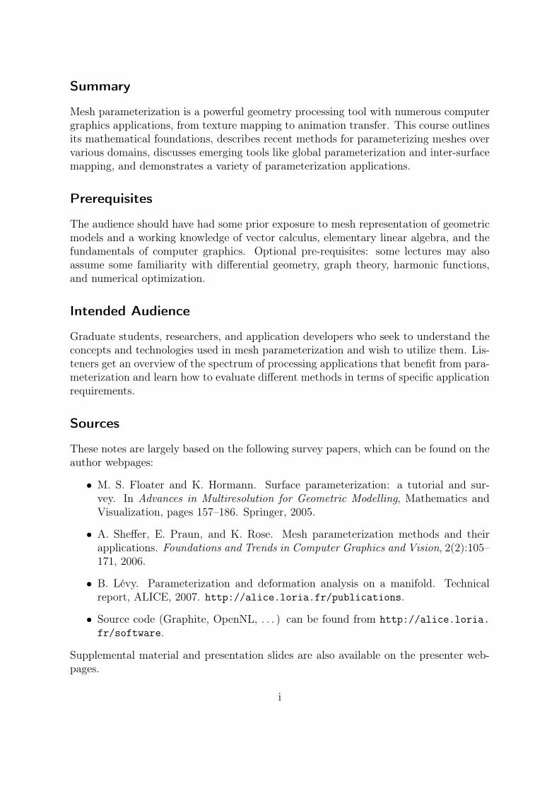
Texture Mapping Normal Mapping Detail Transfer

Morphing Mesh Completion Editing

Databases Remeshing Surface Fitting

Figure 1.1: Parameterization Applications.

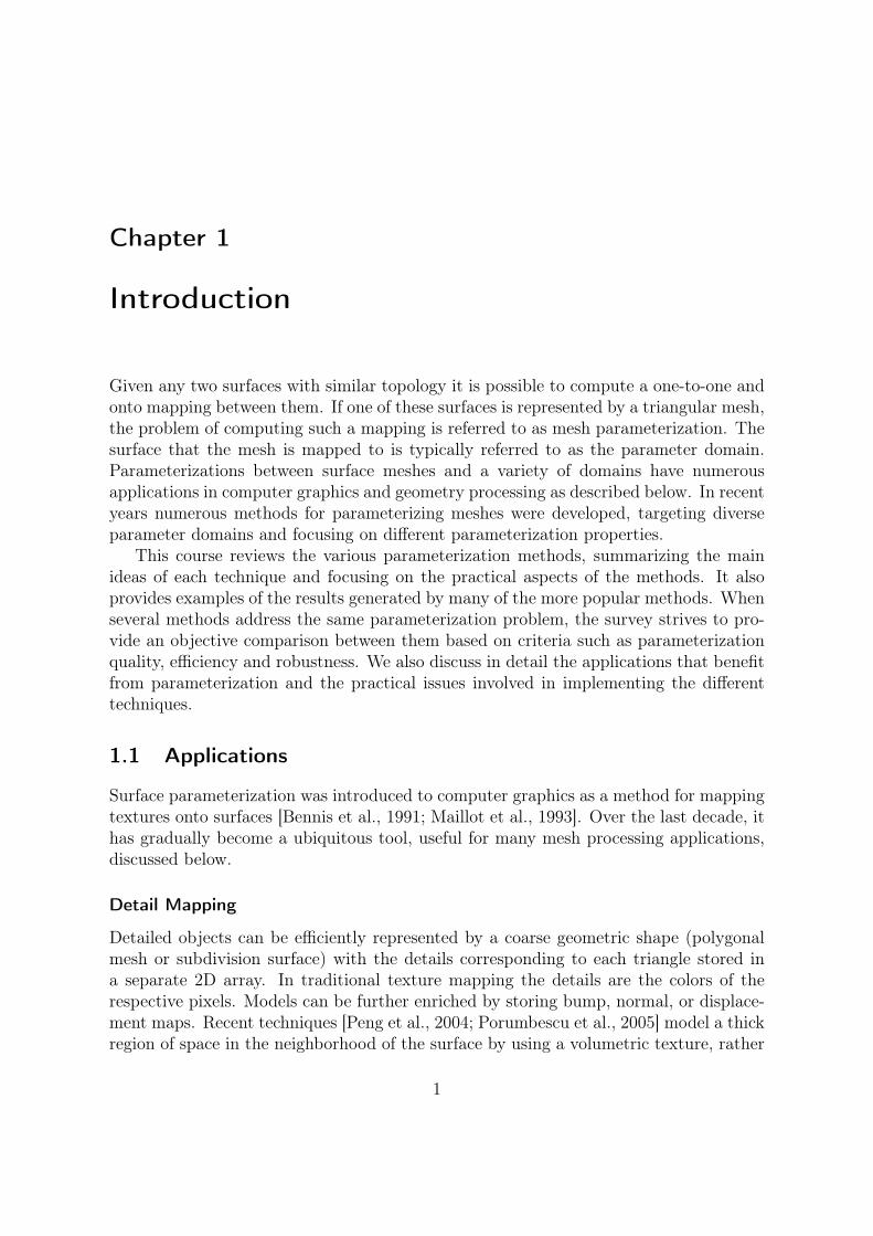
Figure 1.2: Application of parameterization: texture mapping (Least Squares ConformalMaps implemented in the Open-Source Blender modeler).

2

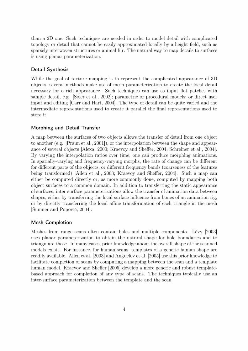
Figure 1.3: Application of parameterization: appearance-preserving simplification. Allthe details are encoded in a normal map, applied onto a dramatically simplified versionof the model (1.5% of the original size).

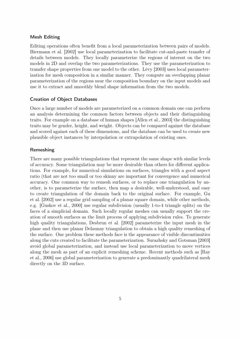
Figure 1.4: A global parameterization realizes an abstraction of the initial geometry.This abstraction can then be re-instanciated into alternative shape representations.

3

than a 2D one. Such techniques are needed in order to model detail with complicatedtopology or detail that cannot be easily approximated locally by a height field, such assparsely interwoven structures or animal fur. The natural way to map details to surfacesis using planar parameterization.

Detail Synthesis

While the goal of texture mapping is to represent the complicated appearance of 3Dobjects, several methods make use of mesh parameterization to create the local detailnecessary for a rich appearance. Such techniques can use as input flat patches withsample detail, e.g. [Soler et al., 2002]; parametric or procedural models; or direct userinput and editing [Carr and Hart, 2004]. The type of detail can be quite varied and theintermediate representations used to create it parallel the final representations used tostore it.

Morphing and Detail Transfer

A map between the surfaces of two objects allows the transfer of detail from one objectto another (e.g. [Praun et al., 2001]), or the interpolation between the shape and appear-ance of several objects [Alexa, 2000; Kraevoy and Sheffer, 2004; Schreiner et al., 2004].By varying the interpolation ratios over time, one can produce morphing animations.In spatially-varying and frequency-varying morphs, the rate of change can be differentfor different parts of the objects, or different frequency bands (coarseness of the featuresbeing transformed) [Allen et al., 2003; Kraevoy and Sheffer, 2004]. Such a map caneither be computed directly or, as more commonly done, computed by mapping bothobject surfaces to a common domain. In addition to transferring the static appearanceof surfaces, inter-surface parameterizations allow the transfer of animation data betweenshapes, either by transferring the local surface influence from bones of an animation rig,or by directly transferring the local affine transformation of each triangle in the mesh[Sumner and Popović, 2004].

Mesh Completion

Meshes from range scans often contain holes and multiple components. Lévy [2003]uses planar parameterization to obtain the natural shape for hole boundaries and totriangulate those. In many cases, prior knowledge about the overall shape of the scannedmodels exists. For instance, for human scans, templates of a generic human shape arereadily available. Allen et al. [2003] and Anguelov et al. [2005] use this prior knowledge tofacilitate completion of scans by computing a mapping between the scan and a templatehuman model. Kraevoy and Sheffer [2005] develop a more generic and robust template-based approach for completion of any type of scans. The techniques typically use aninter-surface parameterization between the template and the scan.

4

Mesh Editing

Editing operations often benefit from a local parameterization between pairs of models.Biermann et al. [2002] use local parameterization to facilitate cut-and-paste transfer ofdetails between models. They locally parameterize the regions of interest on the twomodels in 2D and overlap the two parameterizations. They use the parameterization totransfer shape properties from one model to the other. Lévy [2003] uses local parameter-ization for mesh composition in a similar manner. They compute an overlapping planarparameterization of the regions near the composition boundary on the input models anduse it to extract and smoothly blend shape information from the two models.

Creation of Object Databases

Once a large number of models are parameterized on a common domain one can performan analysis determining the common factors between objects and their distinguishingtraits. For example on a database of human shapes [Allen et al., 2003] the distinguishingtraits may be gender, height, and weight. Objects can be compared against the databaseand scored against each of these dimensions, and the database can be used to create newplausible object instances by interpolation or extrapolation of existing ones.

Remeshing

There are many possible triangulations that represent the same shape with similar levelsof accuracy. Some triangulation may be more desirable than others for different applica-tions. For example, for numerical simulations on surfaces, triangles with a good aspectratio (that are not too small or too skinny are important for convergence and numericalaccuracy. One common way to remesh surfaces, or to replace one triangulation by an-other, is to parameterize the surface, then map a desirable, well-understood, and easyto create triangulation of the domain back to the original surface. For example, Guet al. [2002] use a regular grid sampling of a planar square domain, while other methods,e.g. [Guskov et al., 2000] use regular subdivision (usually 1-to-4 triangle splits) on thefaces of a simplicial domain. Such locally regular meshes can usually support the cre-ation of smooth surfaces as the limit process of applying subdivision rules. To generatehigh quality triangulations, Desbrun et al. [2002] parameterize the input mesh in theplane and then use planar Delaunay triangulation to obtain a high quality remeshing ofthe surface. One problem these methods face is the appearance of visible discontinuitiesalong the cuts created to facilitate the parameterization. Surazhsky and Gotsman [2003]avoid global parameterization, and instead use local parameterization to move verticesalong the mesh as part of an explicit remeshing scheme. Recent methods such as [Rayet al., 2006] use global parameterization to generate a predominantly quadrilateral meshdirectly on the 3D surface.

5

Mesh Compression

Mesh compression is used to compactly store or transmit geometric models. As withother data, compression rates are inversely proportional to the data entropy. Thus highercompression rates can be obtained when models are represented by meshes that are asregular as possible, both topologically and geometrically. Topological regularity refersto meshes where almost all vertices have the same degree. Geometric regularity impliesthat triangles are similar to each other in terms of shape and size and vertices are closeto the centroid of their neighbors. Such meshes can be obtained by parameterizing theoriginal objects and then remeshing with regular sampling patterns [Gu et al., 2002].The quality of the parameterization directly impacts the compression efficiency.

Surface Fitting

One of the earlier applications of mesh parameterization is surface fitting [Floater, 2000].Many applications in geometry processing require a smooth analytical surface to beconstructed from an input mesh. A parameterization of the mesh over a base domainsignificantly simplifies this task. Earlier methods either parameterized the entire meshin the plane or segmented it and parameterized each patch independently. More recentmethods, e.g. [Li et al., 2006] focus on constructing smooth global parameterizationsand use those for fitting, achieving global continuity of the constructed surfaces.

Modeling from Material Sheets

While computer graphics focuses on virtual models, geometry processing has numerousreal-world engineering applications. Particularly, planar mesh parameterization is animportant tool when modeling 3D objects from sheets of material, ranging from garmentmodeling to metal forming or forging [Bennis et al., 1991; Julius et al., 2005]. All ofthese applications require the computation of planar patterns to form the desired 3Dshapes. Typically, models are first segmented into nearly developable charts, and thesecharts are then parameterized in the plane.

Medical Visualization

Complex geometric structures are often better visualized and analyzed by mapping thesurface normal-map, color, and other properties to a simpler, canonical domain. One ofthe structures for which such mapping is particularly useful is the human brain [Hurdalet al., 1999; Haker et al., 2000]. Most methods for brain mapping use the fact that thebrain has genus zero, and visualize it through spherical [Haker et al., 2000] or planar[Hurdal et al., 1999] parameterization.

6

Chapter 2

Differential Geometry Primer

Before we go into the details of how to compute a mesh parameterization and what todo with it, let us quickly review some of the basic properties from differential geometrythat will be essential for understanding the motivation behind the methods describedlater. For more details and proofs of these properties, we refer the interested readerto the standard literature on differential geometry and in particular to the books bydo Carmo [1976], Klingenberg [1978], Kreyszig [1991], and Morgan [1998].

2.1 Basic Definitions

Suppose that Ω ⊂ R2 is some simply connected region (i.e., without any holes), for

example,

the unit square: Ω = (u, v) ∈ R2 : u, v ∈ [0, 1], or

the unit disk : Ω = (u, v) ∈ R2 : u2 + v2 ≤ 1,

and that the function f : Ω → R3 is continuous and an injection (i.e., no two distinct

points in Ω are mapped to the same point in R3). We then call the image S of Ω under

f a surface,S = f(Ω) = f(u, v) : (u, v) ∈ Ω,

and say that f is a parameterization of S over the parameter domain Ω. It follows fromthe definition of S that f is actually a bijection between Ω and S and thus admits todefine its inverse f−1 : S → Ω. Here are some examples:

1. simple linear function:

parameter domain: Ω = (u, v) ∈ R2 : u, v ∈ [0, 1]

surface: S = (x, y, z) ∈ R3 : x, y, z ∈ [0, 1], x + y = 1

parameterization: f(u, v) = (u, 1− u, v)

inverse: f−1(x, y, z) = (x, z)

7

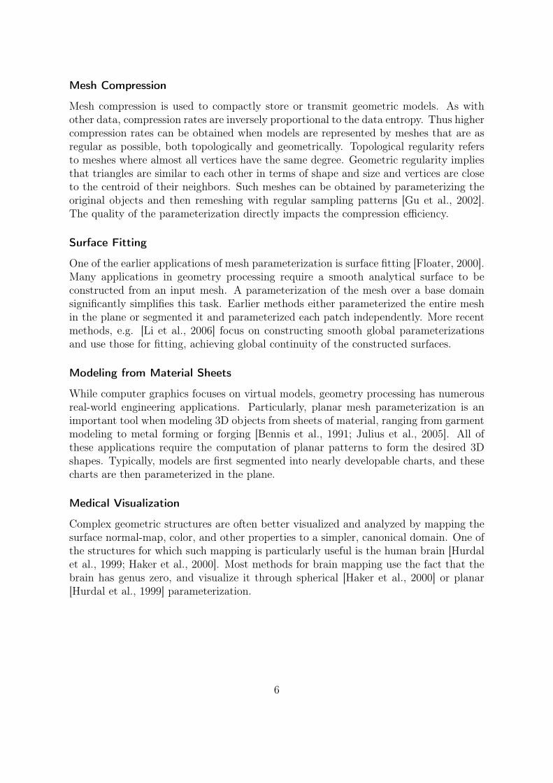
2. cylinder:

parameter domain: Ω = (u, v) ∈ R2 : u ∈ [0, 2π), v ∈ [0, 1]

surface: S = (x, y, z) ∈ R3 : x2 + y2 = 1, z ∈ [0, 1]

parameterization: f(u, v) = (cos u, sin u, v)

inverse: f−1(x, y, z) = (arccos x, z)

3. paraboloid:

parameter domain: Ω = (u, v) ∈ R2 : u, v ∈ [−1, 1]

surface: S = (x, y, z) ∈ R3 : x, y ∈ [−2, 2], z = 1

4(x2 + y2)

parameterization: f(u, v) = (2u, 2v, u2 + v2)

inverse: f−1(x, y, z) = (x2, y

2)

8

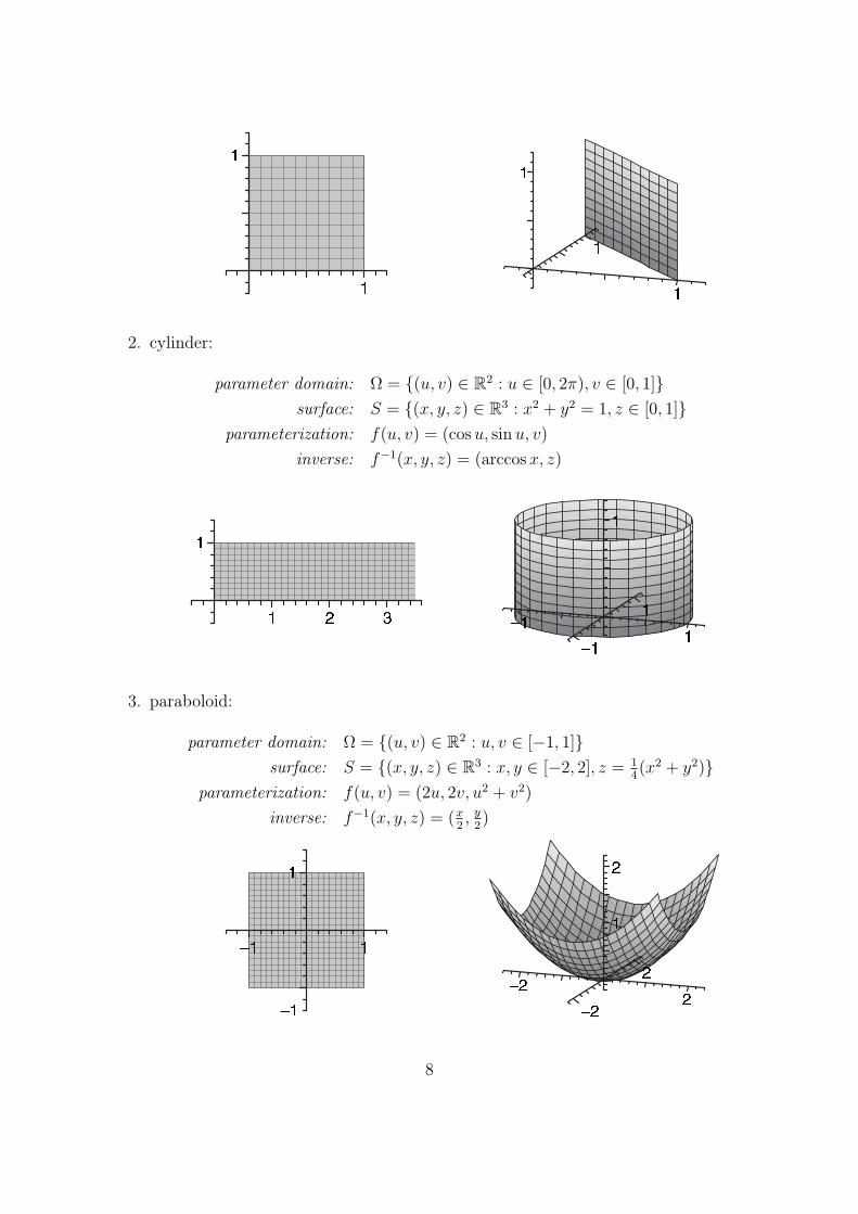
4. hemisphere (orthographic):

parameter domain: Ω = (u, v) ∈ R2 : u2 + v2 ≤ 1

surface: S = (x, y, z) ∈ R3 : x2 + y2 + z2 = 1, z ≥ 0

parameterization: f(u, v) = (u, v,√

1− u2 − v2)

inverse: f−1(x, y, z) = (x, y)

Having defined a surface S like that, we should note that the function f is by nomeans the only parameterization of S over Ω. In fact, given any bijection ϕ : Ω → Ω,it is easy to verify that the composition of f and ϕ, i.e., the function g = f ϕ, isa parameterization of S over Ω, too. For example, we can easily construct such areparameterization ϕ from any bijection ρ : [0, 1]→ [0, 1] by defining

for the unit square: ϕ(u, v) = (ρ(u), ρ(v)), orfor the unit disk: ϕ(u, v) = (uρ(u2 + v2), vρ(u2 + v2)).

In particular, taking the function ρ(x) = 21+x

and applying this reparameterization ofthe unit disk to the parameterization of the hemisphere in the example above gives thefollowing alternative parameterization:

5. hemisphere (stereographic):

parameter domain: Ω = (u, v) ∈ R2 : u2 + v2 ≤ 1

surface: S = (x, y, z) ∈ R3 : x2 + y2 + z2 = 1, z ≥ 0

parameterization: f(u, v) = ( 2u1+u2+v2 ,

2v1+u2+v2 ,

1−u2−v2

1+u2+v2 )

inverse: f−1(x, y, z) = ( x1+z

, y1+z

)

9

2.2 Intrinsic Surface Properties

Although the parameterization of a surface is not unique—and we will later discuss howto get the “best” parameterization with respect to certain criteria—it nevertheless is avery handy thing to have as it allows to compute a variety of properties of the surface.For example, if f is differentiable, then its partial derivatives

fu =∂f

∂uand fv =

∂f

∂v

span the local tangent plane and by simply taking their cross product and normalizingthe result we get the surface normal

nf =fu × fv

‖fu × fv‖.

To simplify the notation, we will often speak of fu and fv as the derivatives and of nf

as the surface normal, but we should keep in mind that formally all three are functionsfrom R

2 to R3. In other words, for any point (u, v) ∈ Ω in the parameter domain, the

tangent plane at the surface point f(u, v) ∈ S is spanned by the two vectors fu(u, v)and fv(u, v), and nf (u, v) is the normal vector at this point1. Again, let us clarify thisby considering two examples:

1. For the simple linear function f(u, v) = (u, 1− u, v) we get

fu(u, v) = (1,−1, 0) and fv(u, v) = (0, 0, 1)

and furthernf (u, v) = (−1√

2, 1√

2, 0),

showing that the normal vector is constant for all points on S.

2. For the parameterization of the cylinder, f(u, v) = (cos u, sin u, v), we get

fu(u, v) = (− sin u, cos u, 0) and fv(u, v) = (0, 0, 1)

and furthernf (u, v) = (cos u, sin u, 0),

showing that the normal vector at any point (x, y, z) ∈ S is just (x, y, 0).

Note that in both examples the surface normal is independent of the parameterization.In fact, this holds for all surfaces and is therefore called an intrinsic property of thesurface. Formally, we can also say that the surface normal is a function n : S → S

2,where S

2 = (x, y, z) ∈ R3 : x2 + y2 + z2 = 1 is the unit sphere in R

3, so that

n(p) = nf (f−1(p))

1We tacitly assume that the parameterization is regular, i.e., fu and fv are always linearly indepen-dent and therefore nf is non-zero.

10

for any p ∈ S and any parameterization f . As an exercise, you may want to verify thisfor the two alternative parameterizations of the hemisphere given above. Other intrinsicsurface properties are the Gaussian curvature K(p) and the mean curvature H(p) aswell as the total area of the surface A(S). To compute the latter, we need the firstfundamental form

If =

(fu · fu fu · fv

fv · fu fv · fv

)=

(E FF G

),

where the product between the partial derivatives is the usual dot product in R3. It

follows immediately from the Cauchy-Schwarz inequality that the determinant of thissymmetric 2 × 2 matrix is always non-negative, so that its square root is always real.The area of the surface is then defined as

A(S) =

∫Ω

√det If du dv.

Take, for example, the orthographic parameterization f(u, v) = (u, v,√

1− u2 − v2)of the hemisphere over the unit disk. After some simplifications we find that

det If =1

1− u2 − v2

and can compute the area of the hemisphere as follows:

A(S) =

1∫−1

√1−v2∫

−√

1−v2

1√1− u2 − v2

du dv

=

1∫−1

[arcsin

u√1− v2

]√1−v2

−√

1−v2

dv

=

1∫−1

π dv

= 2π,

as expected. Of course we get the same result if we use the stereographic parameteriza-tion, and you may want to try that as an exercise.

In order to compute the curvatures we must first assume the parameterization to betwice differentiable, so that its second order partial derivatives

fuu =∂2f

∂u2, fuv =

∂2f

∂u∂v, and fvv =

∂2f

∂v2

are well defined. Taking the dot products of these derivatives with the surface normalthen gives the symmetric 2× 2 matrix that is known as the second fundamental form

IIf =

(fuu · nf fuv · nf

fuv · nf fvv · nf

)=

(L MM N

).

11

Gaussian and mean curvature are finally defined as the determinant and half the traceof the matrix I−1

f IIf , respectively:

K = det(I−1f IIf ) =

det IIf

det If

=LN −M2

EG− F 2

andH = 1

2trace(I−1

f IIf ) =LG− 2MF + NE

2(EG− F 2).

For example, carrying out these computations reveals that the curvatures are constantfor most of the surfaces from above:

simple linear function: K = 0, H = 0,

cylinder: K = 0, H = 12,

hemisphere: K = 1, H = −1.

As an exercise, show that the curvatures at any point p = (x, y, z) of the paraboloidfrom above are K(p) = 1

4(1+z)2and H(p) = 2+z

4(1+z)3/2 .

2.3 Metric Distortion

Apart from these intrinsic surface properties, there are others that depend on the pa-rameterization, most importantly the metric distortion. Consider, for example, the twoparameterizations of the hemisphere above. In both cases, the image of the surface onthe right is overlaid by a regular grid, which actually is the image of the correspondinggrid in the parameter domain shown on the left. You will notice that the surface gridlooks more regular for the stereographic than for the orthographic projection and thatthe latter considerably stretches the grid in the radial direction near the boundary.

To better understand this kind of stretching, let us see what happens to the surfacepoint f(u, v) as we move a tiny little bit away from (u, v) in the parameter domain. Ifwe denote this infinitesimal parameter displacement by (∆u, ∆v), then the new surfacepoint f(u + ∆u, v + ∆v) is approximately given by the first order Taylor expansion f off around (u, v),

f(u + ∆u, v + ∆v) = f(u, v) + fu(u, v)∆u + fv(u, v)∆v.

This linear function maps all points in the vicinity of u = (u, v) into the tangent planeTp at p = f(u, v) ∈ S and transforms circles around u into ellipses around p (seeFigure 2.1). The latter property becomes obvious if we write the Taylor expansion morecompactly as

f(u + ∆u, v + ∆v) = p + Jf (u)(∆u∆v

),

where Jf = (fu fv) is the Jacobian of f , i.e. the 3×2 matrix with the partial derivativesof f as column vectors. Then using the singular value decomposition of the Jacobian,

Jf = UΣV T = U

(σ1 0

0 σ2

0 0

)V T ,

12

Figure 2.1: First order Taylor expansion f of the parameterization f .

Figure 2.2: SVD decomposition of the mapping f .

with singular values σ1 ≥ σ2 > 0 and orthonormal matrices U ∈ R3×3 and V ∈ R

2×2

with column vectors U1, U2, U3, and V1, V2, respectively, we can split up the linear trans-formation f as shown in Figure 2.2:

1. The transformation V T first rotates all points around u such that the vectors V1

and V2 are in alignment with the u- and the v-axes afterwards.

2. The transformation Σ then stretches everything by the factor σ1 in the u- and byσ2 in the v-direction.

3. The transformation U finally maps the unit vectors (1, 0) and (0, 1) to the vectorsU1 and U2 in the tangent plane Tp at p.

As a consequence, any circle of radius r around u will be mapped to an ellipse withsemi-axes of length rσ1 and rσ2 around p and the orthonormal frame [V1, V2] is mappedto the orthogonal frame [σ1U1, σ2U2].

This transformation of circles into ellipses is called local metric distortion of theparameterization as it shows how f behaves locally around some parameter point u ∈ Ωand the corresponding surface point p = f(u) ∈ S. Moreover, all information aboutthis local metric distortion is hidden in the singular values σ1 and σ2. For example, ifboth values are identical, then Jf is just a rotation plus uniform scaling and f does notdistort angles around u. Likewise, if the product of the singular values is 1, then thearea of any circle in the parameter domain is identical to the area of the correspondingellipse in the tangent plane and we say that f is locally area-preserving.

Computing the singular values directly is a bit tedious, so that we better resort tothe fact that the singular values of any matrix A are the square roots of the eigenvaluesof the matrix AT A. In our case, the matrix Jf

T Jf is an old acquaintance, namely the

13

first fundamental form,

JfT Jf =

(fu

T

fvT

)(fu fv) = If =

(E FF G

),

and we can easily compute the two eigenvalues λ1 and λ2 of this symmetric matrix byusing the nifty little formula

λ1,2 = 12

((E + G)±

√4F 2 + (E −G)2

).

We now summarize the main properties that a parameterization can have locally:

f is isometric or length-preserving ⇐⇒ σ1 = σ2 = 1 ⇐⇒ λ1 = λ2 = 1,

f is conformal or angle-preserving ⇐⇒ σ1 = σ2 ⇐⇒ λ1 = λ2,

f is equiareal or area-preserving ⇐⇒ σ1σ2 = 1 ⇐⇒ λ1λ2 = 1.

Obviously, any isometric mapping is conformal and equiareal, and every mapping thatis conformal and equiareal is also isometric, in short,

isometric ⇐⇒ conformal + equiareal.

Thus equipped, let us go back to the examples above and check their properties:

1. simple linear function:

parameterization: f(u, v) = (u, 1− u, v)

Jacobian: Jf =(

1 0−1 00 1

)first fundamental form: If =

(2 00 1

)eigenvalues: λ1 = 2, λ2 = 1

This parameterization is neither conformal nor equiareal.

2. cylinder:

parameterization: f(u, v) = (cos u, sin u, v)

Jacobian: Jf =(

cos u 0− sin u 0

0 1


(1 00 1

)eigenvalues: λ1 = 1, λ2 = 1

This parameterization is isometric.

14

3. paraboloid:

parameterization: f(u, v) = (2u, 2v, u2 + v2)

Jacobian: Jf =(

2 00 22u 2v


(4+4u2 4uv

4uv 4+4v2

)eigenvalues: λ1 = 4, λ2 = 4(1 + u2 + v2)

This mapping is not equiareal and conformal only at (u, v) = (0, 0).

4. hemisphere (orthographic):

parameterization: f(u, v) = (u, v, 1d) with d = 1√

1−u2−v2

Jacobian: Jf =( 1 0

0 1−ud −vd


(1+u2d2 uvd2

uvd2 1+v2d2

)eigenvalues: λ1 = 1, λ2 = d2

This mapping is isometric at (u, v) = (0, 0), but neither conformal nor equiarealelsewhere.

5. hemisphere (stereographic):

parameterization: f(u, v) = (2ud, 2vd, (1− u2 − v2)d) with d = 11+u2+v2

Jacobian: Jf =

(2d−4u2d2 −4uvd2

−4uvd2 2d−4v2d2

−4ud2 −4vd2


(4d2 00 4d2

)eigenvalues: λ1 = 4d2, λ2 = 4d2

This mapping is always conformal, but equiareal and thus isometric only at theboundary of Ω, i.e., for u2 + v2 = 1.

It turns out that the only parameterization that is optimal in the sense that it isisometric everywhere and thus does not introduce any distortion at all is the one for thecylinder. In fact, it was shown by Gauß [1827] that a globally isometric parameteriza-tion exists only for developable surfaces like planes, cones, and cylinders with vanishingGaussian curvature K(p) = 0 at all surface points p ∈ S. As an exercise, you can tryto find such a globally isometric parameterization for the planar surface patch from thefirst example.

Other interesting parameterizations are those that are globally conformal like thestereographic projection for the hemisphere, and it was shown by Riemann [1851] that

15

such a parameterization exists for any surface that is topologically equivalent to a diskand any simply connected parameter domain.

More generally, the “best” parameterization f of a surface S over a parameter domainΩ is found as follows. We first need a bivariate non-negative function E : R

2+ → R+

that measures the local distortion of a parameterization with singular values σ1 andσ2. Usually, this function has a global minimum at (1, 1) so as to favour isometry, butdepending on the application, it may also be defined such that the minimal value istaken along the whole line (x, x) for x ∈ R+, for example, if conformal mappings shallbe preferred. The overall distortion of a particular parameterization f is then measuredby simply averaging the local distortion over the whole domain,

E(f) =

∫Ω

E(σ1(u, v), σ2(u, v)) du dv/

A(Ω),

and the best parameterization with respect to E is then found by minimizing E(f) overthe space of all admissible parameterizations.

16

Chapter 3

Barycentric Mappings

In many applications, and in particular in computer graphics, it is nowadays commonto work with piecewise linear surfaces in the form of triangle meshes, and we will mainlystick to this type of surface for the remainder of these course notes.

3.1 Triangle Meshes

As in the previous chapter, let us denote points in R3 by p = (x, y, z) and points in

R2 by u = (u, v). An edge is then defined as the convex hull of (or, equivalently, the

line segment between) two distinct points and a triangle as the convex hull of threenon-collinear points. We will denote edges and triangles in R

3 with capital letters andthose in R

2 with small letters, for example, e = [u1, u2] and T = [p1, p2, p3].A triangle mesh ST is the union of a set of surface triangles T = T1, . . . , Tm which

intersect only at common edges E = E1, . . . , El and vertices V = p1, . . . ,pn+b. Morespecifically, the set of vertices consists of n interior vertices VI = p1, . . . ,pn and bboundary vertices VB = pn+1, . . . ,pn+b. Two distinct vertices pi, pj ∈ V are calledneighbours, if they are the end points of some edge E = [pi, pj] ∈ E , and for any pi ∈ Vwe let Ni = j : [pi, pj] ∈ E be the set of indices of all neighbours of pi.

A parameterization f of ST is usually specified the other way around, that is, bydefining the inverse parameterization g = f−1. This mapping g is uniquely determinedby specifying the parameter points ui = g(pi) for each vertex pi ∈ V and demanding thatg is continuous and linear for each triangle. In this setting, g|T is the linear map from asurface triangle T = [pi, pj, pk] to the corresponding parameter triangle t = [ui, uj, uk]

and f |t = (g|T )−1 is the inverse linear map from t to T . The parameter domain Ω finallyis the union of all parameter triangles (see Figure 3.1).

3.2 Parameterization by Affine Combinations

A rather simple idea for constructing a parameterization of a triangle mesh is based onthe following physical model. Imagine that the edges of the triangle mesh are springsthat are connected at the vertices. If we now fix the boundary of this spring networksomewhere in the plane, then the interior of this network will relax in the energetically

17

ST

Ω

f|t

t T

g|T

Figure 3.1: Parameterization of a triangle mesh.

most efficient configuration, and we can simply assign the positions where the joints ofthe network have come to rest as parameter points.

If we assume each spring to be ideal in the sense that the rest length is zero and thepotential energy is just 1

2Ds2, where D is the spring constant and s the length of the

spring, then we can formalize this approach as follows. We first specify the parameterpoints ui = (ui, vi), i = n + 1, . . . , n + b for the boundary vertices pi ∈ VB of the meshin some way (see Section 3.4). Then we minimize the overall spring energy

E = 12

n∑i=1

∑j∈Ni

12Dij‖ui − uj‖2,

where Dij = Dji is the spring constant of the spring between pi and pj, with respectto the unknown parameter positions ui = (ui, vi) for the interior points1. As the partialderivative of E with respect to ui is

∂E

∂ui

=∑j∈Ni

Dij(ui − uj),

the minimum of E is obtained if∑j∈Ni

Dijui =∑j∈Ni

Dijuj

holds for all i = 1, . . . , n. This is equivalent to saying that each interior parameter pointui is an affine combination of its neighbours,

ui =∑j∈Ni

λijuj, (3.1)

with normalized coefficientsλij = Dij

/∑k∈Ni

Dik

that obviously sum to 1.1The additional factor 1

2 appears because summing up the edges in this way counts every edge twice.

18

By separating the parameter points for the interior and the boundary vertices in thesum on the right hand side of (3.1) we get

ui −∑

j∈Ni,j≤n

λijuj =∑

j∈Ni,j>n

λijuj,

and see that computing the coordinates ui and vi of the interior parameter points ui

requires to solve the linear systems

AU = U and AV = V , (3.2)

where U = (u1, . . . , un) and V = (v1, . . . , vn) are the column vectors of unknown coordi-nates, U = (u1, . . . , un) and V = (v1, . . . , vn) are the column vectors with coefficients

ui =∑

j∈Ni,j>n

λijuj and vi =∑

j∈Ni,j>n

λijvj

and A = (aij)i,j=1,...,n is the n× n matrix with elements

aij =

⎧⎪⎨⎪⎩

1 if i = j,

−λij if j ∈ Ni,

0 otherwise.

Methods for efficiently solving these systems are described in Chapter 10 of these coursenotes.

3.3 Barycentric Coordinates

The question remains how to choose the spring constants Dij in the spring model, ormore generally, the normalized coefficients λij in (3.1). The simplest choice of constantspring constants Dij = 1 goes back to the work of Tutte [1960, 1963] who used it ina more abstract graph-theoretic setting to compute straight line embeddings of planargraphs, and the idea of taking spring constants that are proportional to the lengths ofthe corresponding edges in the triangle mesh was used by Greiner and Hormann [1997].A main drawback of both approaches is that they do not fulfill the following minimumrequirement that we should expect from any parameterization method.

Linear reproduction: Suppose that ST is contained in a plane so that its verticeshave coordinates pi = (xi, yi, 0) with respect to some appropriately chosen orthonormalcoordinate frame. Then a globally isometric (and thus optimal) parameterization can bedefined by just using the local coordinates xi = (xi, yi) as parameter points themselves,that is, by setting ui = xi for i = 1, . . . , n + b. As the overall parameterization then isa linear function, we say that a parameterization method has linear reproduction if itproduces such an isometric mapping in this setting.

19

Figure 3.2: Notation for the construction of barycentric coordinates.

In the setting from the previous section, linear reproduction can be achieved if theparameter points for the boundary vertices are set correctly and the values λij are chosensuch that

xi =∑j∈Ni

λijxj and∑j∈Ni

λij = 1

for all interior vertices. Values λij with both these properties are also called barycentriccoordinates of xi with respect to its neighbours xj, j ∈ Ni. If some xi has exactly threeneighbours, then the λij are uniquely defined and these barycentric coordinates insidetriangles actually have many useful applications in computer graphics (e.g., Gouraud andPhong shading, ray-triangle-intersection), geometric modelling (e.g., triangular Bézierpatches, splines over triangulations), and many other fields (e.g., the finite elementmethod, terrain modelling).

For polygons with more than three vertices, the barycentric coordinates of a pointin the interior are, however, not unique anymore and there are several ways of definingthem. The most popular of them can all be described in a common framework [Floateret al., 2006] that we shall briefly review. For any interior point xi and one of its neigh-bours xj let rij = ‖xi − xj‖ be the length of the edge eij = [xi, xj] between the twopoints and let the angles at the corners of the triangles adjacent to eij be denoted asshown in Figure 3.2. The barycentric coordinates λij of xi with respect its neighboursxj, j ∈ Ni can then be computed by the normalization λij = wij

/∑k∈Ni

wik from anyof the following homogeneous coordinates wij.

• Wachspress coordinates: The earliest generalization of barycentric coordinates goesback to Wachspress [1975] who suggested to set

wij =cot αji + cot βij

rij2

.

While he was mainly interested in applying these coordinates in finite elementmethods, Desbrun et al. [2002] used them for parameterizing triangle meshes andMeyer et al. [2002] for interpolating e.g. colour values inside convex polygons.Moreover, a simple geometric construction of these coordinates was given by Juet al. [2005b].

20

p2 = (-1,-1,0) p3 = (1,-1,0)

p4 = (1,1,0)p5 = (-1,1,0)

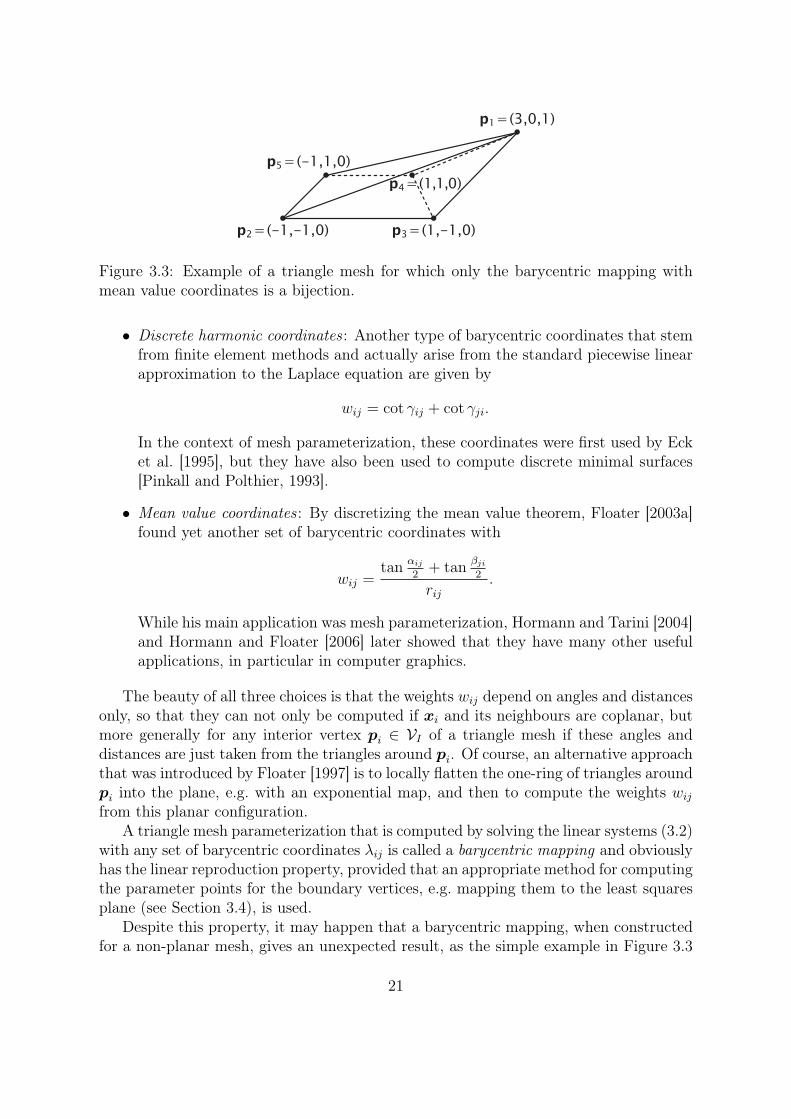
p1 = (3,0,1)

Figure 3.3: Example of a triangle mesh for which only the barycentric mapping withmean value coordinates is a bijection.

• Discrete harmonic coordinates: Another type of barycentric coordinates that stemfrom finite element methods and actually arise from the standard piecewise linearapproximation to the Laplace equation are given by

wij = cot γij + cot γji.

In the context of mesh parameterization, these coordinates were first used by Ecket al. [1995], but they have also been used to compute discrete minimal surfaces[Pinkall and Polthier, 1993].

• Mean value coordinates: By discretizing the mean value theorem, Floater [2003a]found yet another set of barycentric coordinates with

wij =tan

αij

2+ tan

βji

2

rij

.

While his main application was mesh parameterization, Hormann and Tarini [2004]and Hormann and Floater [2006] later showed that they have many other usefulapplications, in particular in computer graphics.

The beauty of all three choices is that the weights wij depend on angles and distancesonly, so that they can not only be computed if xi and its neighbours are coplanar, butmore generally for any interior vertex pi ∈ VI of a triangle mesh if these angles anddistances are just taken from the triangles around pi. Of course, an alternative approachthat was introduced by Floater [1997] is to locally flatten the one-ring of triangles aroundpi into the plane, e.g. with an exponential map, and then to compute the weights wij

from this planar configuration.A triangle mesh parameterization that is computed by solving the linear systems (3.2)

with any set of barycentric coordinates λij is called a barycentric mapping and obviouslyhas the linear reproduction property, provided that an appropriate method for computingthe parameter points for the boundary vertices, e.g. mapping them to the least squaresplane (see Section 3.4), is used.

Despite this property, it may happen that a barycentric mapping, when constructedfor a non-planar mesh, gives an unexpected result, as the simple example in Figure 3.3

21

x4 = (-1,-1)

x5 = (1,0)

x6 = (-1,1)

x7 = (-1/3,0)

x1 = (-1/5,0)

x3 = (1/3,0)

x2 = (0,0)

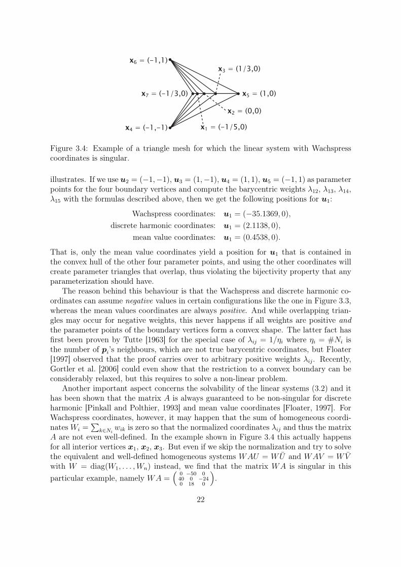
Figure 3.4: Example of a triangle mesh for which the linear system with Wachspresscoordinates is singular.

illustrates. If we use u2 = (−1,−1), u3 = (1,−1), u4 = (1, 1), u5 = (−1, 1) as parameterpoints for the four boundary vertices and compute the barycentric weights λ12, λ13, λ14,λ15 with the formulas described above, then we get the following positions for u1:

Wachspress coordinates: u1 = (−35.1369, 0),

discrete harmonic coordinates: u1 = (2.1138, 0),

mean value coordinates: u1 = (0.4538, 0).

That is, only the mean value coordinates yield a position for u1 that is contained inthe convex hull of the other four parameter points, and using the other coordinates willcreate parameter triangles that overlap, thus violating the bijectivity property that anyparameterization should have.

The reason behind this behaviour is that the Wachspress and discrete harmonic co-ordinates can assume negative values in certain configurations like the one in Figure 3.3,whereas the mean values coordinates are always positive. And while overlapping trian-gles may occur for negative weights, this never happens if all weights are positive andthe parameter points of the boundary vertices form a convex shape. The latter fact hasfirst been proven by Tutte [1963] for the special case of λij = 1/ηi where ηi = #Ni isthe number of pi’s neighbours, which are not true barycentric coordinates, but Floater[1997] observed that the proof carries over to arbitrary positive weights λij. Recently,Gortler et al. [2006] could even show that the restriction to a convex boundary can beconsiderably relaxed, but this requires to solve a non-linear problem.

Another important aspect concerns the solvability of the linear systems (3.2) and ithas been shown that the matrix A is always guaranteed to be non-singular for discreteharmonic [Pinkall and Polthier, 1993] and mean value coordinates [Floater, 1997]. ForWachspress coordinates, however, it may happen that the sum of homogeneous coordi-nates Wi =

∑k∈Ni

wik is zero so that the normalized coordinates λij and thus the matrixA are not even well-defined. In the example shown in Figure 3.4 this actually happensfor all interior vertices x1, x2, x3. But even if we skip the normalization and try to solvethe equivalent and well-defined homogeneous systems WAU = WU and WAV = WVwith W = diag(W1, . . . , Wn) instead, we find that the matrix WA is singular in thisparticular example, namely WA =

(0 −50 040 0 −240 18 0

).

22

3.4 The Boundary Mapping

The first step in constructing a barycentric mapping is to choose the parameter pointsfor the boundary vertices and the simplest way of doing it is to just project the bound-ary vertices into the plane that fits the boundary vertices best in a least squares sense.However, for meshes with a complex boundary, this simple procedure may lead to un-desirable fold-overs in the boundary polygon and cannot be used. In general, there aretwo issues to take into account here: (1) choosing the shape of the boundary of theparameter domain and (2) choosing the distribution of the parameter points around theboundary.

Choosing the shape

In many applications, it is sufficient (or even desirable) to take a rectangle or a circleas parameter domain, with the advantage that such a convex shape guarantees thebijectivity of the parameterization if positive barycentric coordinates like the mean valuecoordinates are used to compute the parameter points for the interior vertices. Theconvexity restriction may, however, generate big distortions near the boundary whenthe boundary of the triangle mesh ST does not resemble a convex shape. One practicalsolution to avoid such distortions is to build a “virtual” boundary, i.e., to augment thegiven mesh with extra triangles around the boundary so as to construct an extendedmesh with a “nice” boundary. This approach has been successfully used by Lee et al.[2002], and Kós and Várady [2003].

Choosing the distribution

The usual procedure mentioned in the literature is to use a simple univariate parameteri-zation method such as chord length [Ahlberg et al., 1967] or centripetal parameterization[Lee, 1989] for placing the parameter points either around the whole boundary, or alongeach side of the boundary when working with a rectangular domain [Hormann, 2001,Section 1.2.5].

Despite these heuristics working pretty well in some cases, having to fix the boundaryvertices may be a severe limitation in others and the next chapter studies parameteri-zation methods that can include the position of the boundary parameter points in theoptimization process and thus yield parameterizations with less distortion.

23

Chapter 4

Setting the Boundary Free

As explained in the previous section, Tutte’s theorem combined with mean value weightsprovides a provably correct way of constructing a valid parameterization for a disk-likesurface. However, for some surfaces, the necessity to fix the boundary on a convexpolygon may be problematic (c.f. Figure 4.1), for the following reasons : (1) in general,it is difficult to find a “natural” way of fixing the border on a convex polygon, and(2) for some surfaces, the shape of the boundary is far from convex. Therefore theobtained parameterization shows high deformations. Even if one can imagine differentways of improving the result shown in the Figure, the so-obtained parameterization willbe probably not as good as the one shown in Figure 4.1-C, that better matches whata tanner would expect for such a mesh. For these reasons, the next section studiesthe methods that can construct parameterizations with free boundaries, that minimizedeformations in a similar way. We start by giving an intuition of how to use the notionsfrom differential geometry explained in Chapter 2 in our context of parameterizationwith free boundaries.

4.1 Deformation analysis

To see how to apply the theoretic concepts explained in Chapter 2, we first need to grasptheir intuitive meaning.

4.1.1 The Jacobian matrix

The first derivatives of the parameterization are involved in deformation analysis, it isthen necessary to have an intuition of their geometric meaning. In physics, material pointmechanics studies the movement of an object, approximated by a point p, when forcesare applied to it. The trajectory is the curve described by the point p when t varies fromt0 to t1, where t denotes time. The function putting a given time t in correspondencewith the position p(t) = x(t), y(t), z(t) of the point p is a parameterization of thetrajectory, i.e., a parameterization of a curve. It is well known that the vector of thederivatives v(t) = ∂p/∂t = ∂x/∂t, ∂y/∂t, ∂z/∂t corresponds to the speed of p attime t.

24

Figure 4.1: A: a mesh cut in a way that makes it homeomorphic to a disk, using theseamster algorithm [Sheffer and Hart, 2002]; B: Tutte-Floater parameterization obtainedby fixing the border on a square; C: parameterization obtained with a free-boundaryparameterization [Sheffer and de Sturler, 2001].

u

v

ΩRI2 RI

3

S

∂x∂u

∂x∂v

dudv

x(u,v)

ww’

Cu

Cv

Cw

v0

u0

Figure 4.2: Elementary displacements from a point (u, v) of Ω along the u and the v axesare transformed into the tangent vectors to the iso-u and iso-v curves passing throughthe point f(u, v)

25

As shown in Figure 4.2, we consider now a function f : (u, v) → (x, y, z), putting asubspace Ω of R

2 in one-to-one correspondence with a surface S of R3. The scalars (u, v)

are the coordinates in parameter space. In the case of a curve parameterization, thecurve is described by a single parameter t. In contrast, in our case, we consider a surfaceparameterization f(u, v) = x(u, v), y(u, v), z(u, v), and there are two parameters, uand v. Therefore, at a given point (u0, v0) of the parameter space Ω, there are two“speed” vectors to consider: fu = (∂f/∂u)(u0, v0) and fv = (∂f/∂v)(u0, v0). It is easy tocheck that fu is the “speed” vector of the curve Cu : t → f(u0 + t, v0) at X (u0, v0) andthat fv is the “speed” vector of the curve Cv : t → f(u0, v0 + t). The curve Cu (resp.Cv) is the iso-u (resp. the iso-v) curve passing through f(u0, v0), i.e. the image throughf of the line of equation u = u0 (resp. v = v0).

4.1.2 The 1st fundamental form and the anisotropy ellipse

At that point, one may think that the information provided by the two vectors fu(u0, v0)and fv(u0, v0) is not sufficient to characterize the distortions between Ω and S in theneighborhood of (u0, v0) and f(u0, v0). In fact, they can be used to compute how anarbitrary vector w = (a, b) in parameter space is transformed into a vector w′ in theneighborhood of (u0, v0). In other words, we want to compute the “speed” vector w′ =∂f(u0 + t.a, v0 + t.b)/∂t of the curve corresponding to the image of the straight line(u, v) = (u0, v0) + t.w. The vector w′, i.e. the tangent to the curve Cw, can be simplycomputed by applying the chain rule, and one can check that it can be computed fromthe derivatives of f as follows : w′ = afu(u0, v0) + bfv(u0, v0). The vector w′ is referredto as the directional derivative of f at (u0, v0) relative to the direction w.

In matrix form, w′ is obtained by w′ = J(u0, v0)w, where J(u0, v0) is the matrix ofall the partial derivatives of f :

J(u0, v0) =

⎡⎢⎢⎢⎢⎣

∂x∂u

(u0, v0)∂x∂v

(u0, v0)

∂y∂u

(u0, v0)∂y∂v

(u0, v0)

∂z∂u

(u0, v0)∂z∂v

(u0, v0)

⎤⎥⎥⎥⎥⎦ =

[fu(u0, v0)

... fv(u0, v0)

](4.1)

As already said in Chapter 2, the matrix J(u0, v0) is referred to as the Jacobianmatrix of f at (u0, v0).

The notion of directional derivative makes it possible to know what an elementarydisplacement w from a point (u0, v0) in parameter space becomes when it is transformedby the function f . The Jacobian matrix helps also computing dot products and vectornorms onto the surface S. This can be done using the matrix JTJ, referred to as the 1st

fundamental form of f , also described in the differential geometry section. This matrixis denoted by I, and defined by :

I(u0, v0) = JTJ =

⎡⎣ fu · fu fu · fv

fv · fu fv · fv

⎤⎦ (4.2)

26

x(u,v)

u

v

ΩRI2 RI

3

S

dudv

∂x∂u

∂x∂v

Figure 4.3: Anisotropy: an elementary circle is transformed into an elementary ellipse.

The 1st fundamental form I(u0, v0) is also referred to as the metric tensor of f ,since it makes it possible to measure how distances and angles are transformed in theneighborhood of (u0, v0). The squared norm of the image w′ of a vector w is givenby ||w′||2 = wT Iw, and the dot product w′T

1 w′2 = wT

1 Iw2 determines how the anglebetween w1 and w2 is transformed. The next section gives a geometric interpretation ofthe 1st fundamental form and its eigenvalues.

The previous section has studied how an elementary displacement from a parameter-space location (u0, v0) is transformed through the parameterization f . As shown inFigure 4.3, our goal is now to determine what an elementary circle becomes.

Let us consider the two eigenvalues λ1, λ2 of G, and two associated unit eigenvectorsw1,w2. Note that since I is symmetric, w1 and w2 are orthogonal. An arbitrary unitvector w can be written as w = cos(θ)w1 + sin(θ)w2. The squared norm of w′ = Jw isthen given by:

||w′||2 = wT Iw= (cos(θ)w1 + sin(θ)w2)

T I(cos(θ).w1 + sin(θ).w2)= cos2(θ)||w1||2λ1 + sin2(θ)||w1||2λ2+

sin(θ) cos(θ)(λ1wT2 w1 + λ2w

T1 w2)

= cos2(θ).λ1 + sin2(θ).λ2

(4.3)

In Equation 4.3, the cross terms wT1 w2 and wT

2 w1 vanish since w1 and w2 areorthogonal. Let us see now what are the extrema of ||w′||2 in function of θ.

∂||w′(θ)||2∂θ

= 2 sin(θ) cos(θ)(λ2 − λ1)= sin(2θ)(λ2 − λ1)

(4.4)

The extrema of ||w′(θ)||2 are then obtained for θ ∈ 0, π/2, π, 3π/2, i.e. for w = w1

or w = w2. Therefore, the maximum and minimum values of ||w′(θ)||2 are λ1 and λ2,

27

and:

• The axes of the anisotropy ellipse are Jw1 and Jw2;

• The lengths of the axes are√

λ1 and√

λ2.

Note: as mentioned in Chapter 2, the lengths of the axes√

λ1 and√

λ2 also corre-spond to the singular values of the matrix J. A geometric interpretation of the SVD isalso explained in that chapter. We remind that the singular value decomposition (SVD)of a matrix J writes:

J = UΣVT = U

⎡⎢⎢⎢⎢⎣

σ1 0

0 σ2

0 0

⎤⎥⎥⎥⎥⎦VT

where U : 3× 3 and V : 2× 2 are such that their column vectors form an orthonormalbasis (we also say that they are unit matrices), and Σ is a matrix such that only itsdiagonal elementsσ1, σ2 are non-zero. The scalars σ1, σ2 are called the singular values ofJ . In our case, by substituting the Jacobian matrix J with its SVD, we obtain:

I = JTJ

= (UΣVT )T (UΣVT )

= VΣTUTUΣVT = VΣTΣVT

= V

[σ2

1 00 σ2

2

]VT

Since U is a unit matrix, the central term UTU of the third line is equal to the identitymatrix and vanishes. We then obtain SVD of the matrix I, that is also a diagonalizationof I. By unicity of the SVD, we deduce the relation between the eigenvalues λ1, λ2 of Gand the singular values σ1, σ2 of J : λ1 = σ2

1 and λ2 = σ22.

We can now give the expression of the lengths of the anisotropy ellipse σ1 and σ2. Wefirst recall the expression of the Jacobian matrix as a function of the gradient vectors:

I = JTJ =

(E FF G

)with

⎧⎪⎨⎪⎩

E = f 2u

F = fu · fv

G = f 2v

(4.5)

The lengths of the axis of the anisotropy ellipse correspond to the eigenvalues ofI. Their expression can be found by computing the square roots of the zeros of thecharacteristic polynomial |I− σId| (that is a second order equation in σ) :

σ1 =√

1/2(E + G) +√

(E −G)2 + 4F 2

σ2 =√

1/2(E + G)−√

(E −G)2 + 4F 2(4.6)

28

Figure 4.4: Local X, Y basis in a triangle.

Deformation analysis for triangulated surfaces

Deformation analysis, introduced in the previous section, involves the computation ofthe gradients of the parameterization as a function of the parameters u and v. In the caseof a triangulated surface, the parameterization is a piecewise linear function. Therefore,the gradients are constant in each triangle.

Before studying the computation of these gradients, we need to mention that oursetting is slightly different from the previous section. In our case, as previously men-tioned, the 3D surface is given, and our goal is to construct the parameterization. In thissetting, it seems more natural to characterize the inverse of the parameterization, i.e.the function that goes from the 3D surface (known) to the parametric space (unknown).This function is also piecewise linear. To port deformation analysis to this setting, it ispossible to provide each triangle with an orthonormal basis X, Y , as shown in Figure 4.4(and we can use one of the vertices pi of the triangle as the origin). In this basis, wecan study the inverse of the parameterization, that is to say the function that maps apoint (X, Y ) of the triangle to a point (u, v) in parameter space. This function writes :

u(X, Y ) = λ1ui + λ2uj + λ3uk

v(X, Y ) = λ1vi + λ2vj + λ3vk

where (λ1, λ2, λ3) denote the barycentric coordinates at the point (x, y) in the triangle,computed as before :⎛

⎝λi

λj

λk

⎞⎠ =

1

2|T |X,Y

⎛⎝Yj − Yk Xk −Xj XjYk −XkYj

Yk − Yi Xi −Xk XkYi −XiYk

Yi − Yj Xj −Xi XiYj −XjYi

⎞⎠⎛⎝X

Y1

⎞⎠

where 2|T |X,Y = (XiYj − YiXj) + (XjYk − YjXk) + (XkYi − YkXi) denotes the doublearea of the triangle (in 3D space this time).

29

Figure 4.5: Iso-u,v curves and associated gradients.

By substituting the values of λ1, λ2 and λ3 in u = λ1ui + λ2uj + λ3uk (resp. v), weobtain:(

∂u/∂X

∂u/∂Y

)= MT

⎛⎝ui

uj

uk

⎞⎠ =

1

2|T |X,Y

(Yj − Yk Yk − Yi Yi − Yj

Xk −Xj Xi −Xk Xj −Xi

)⎛⎝ui

uj

uk

⎞⎠ (4.7)

where the matrix MT solely depends on the geometry of the triangle T .As shown in Figure 4.5, these gradients are different (but strongly related with) the

gradients of the inverse function, computed in the previous section. The gradient of u( resp. v) intersects the iso-us (resp. the iso-vs) with a right angle (instead of beingtangent to them), and its norm is the inverse of the one computed in the previous section.

30

These gradients can then be used to deduce the expression of the Jacobian matrixJT , as follows :

JT =

(∂u∂X

∂v∂X

∂u∂Y

∂v∂Y

)

= 12|T |x,y

(0 −11 0

)(X3 −X2 X1 −X3 X2 −X1

Y3 − Y2 Y1 − Y3 Y2 − Y1

)⎛⎝u1 v1

u2 v2

u3 v3

⎞⎠

= 12|T |x,y

(0 −11 0

)(X1 X2 X3

Y1 Y2 Y3

)⎛⎝ 0 1 −1−1 0 1

1 −1 0

⎞⎠⎛⎝u1 v1

u2 v2

u3 v3

⎞⎠

(4.8)

The second line of this equation shows how the Jacobian matrix combines the vec-tors of the edges of the triangle with the (u, v) coordinates. The third line is a moresymmetric expression, that uses the coordinates of the points directly. The square ma-trix swaps the coordinates of the triangle edges shows an interesting similarity with theimaginary number i (in fact, this is a representation of the imaginary number i). Wewill elaborate more on the links with complex analysis in Section 4.3 that deals withconformal methods.

4.2 Parameterization methods based on deformation analysis

This section reviews these methods, using the formalism introduced in Chapter 2 andSection 4.1. However, before going further, we need to warn the reader about a possiblesource of confusion :

• half of the methods study the function that goes from the surface to the parametricspace (as in the previous Section). This is justified by the fact that the (u, v)coordinates are unknown. Therefore, it is more natural to go from the knownworld (the surface) to the unknown world (the parameter space);

• the other half of the methods use the inverse convention, and study the functionthat goes from parameter space to the surface (as in Section 4.1). This is justi-fied by the fact that it makes the formalism compatible with classical differentialgeometry books [do Carmo, 1976] that use this convention.

Since both conventions are justified, both are used by different authors. However,as will be shown, deformation analysis for one convention can be easily deduced fromthe other one. Therefore, except the risk of confusion, this does not introduce muchdifficulty to understand these methods. So far, the notations we used in this section arerelated with the function that maps (X, Y ) local coordinates in the triangle to (u, v)coordinates in parameter space Ω.

31

p

qq

q

12

3 p

q...q...

q...

q...

q...

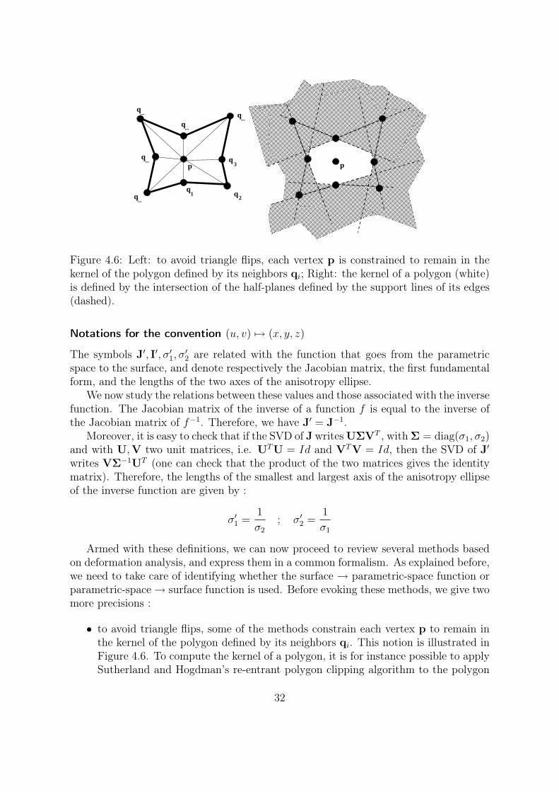
Figure 4.6: Left: to avoid triangle flips, each vertex p is constrained to remain in thekernel of the polygon defined by its neighbors qi; Right: the kernel of a polygon (white)is defined by the intersection of the half-planes defined by the support lines of its edges(dashed).

Notations for the convention (u, v) → (x, y, z)

The symbols J′, I′, σ′1, σ

′2 are related with the function that goes from the parametric

space to the surface, and denote respectively the Jacobian matrix, the first fundamentalform, and the lengths of the two axes of the anisotropy ellipse.

We now study the relations between these values and those associated with the inversefunction. The Jacobian matrix of the inverse of a function f is equal to the inverse ofthe Jacobian matrix of f−1. Therefore, we have J′ = J−1.

Moreover, it is easy to check that if the SVD of J writes UΣVT , with Σ = diag(σ1, σ2)and with U,V two unit matrices, i.e. UTU = Id and VTV = Id, then the SVD of J′

writes VΣ−1UT (one can check that the product of the two matrices gives the identitymatrix). Therefore, the lengths of the smallest and largest axis of the anisotropy ellipseof the inverse function are given by :

σ′1 =

1

σ2

; σ′2 =

1

σ1

Armed with these definitions, we can now proceed to review several methods basedon deformation analysis, and express them in a common formalism. As explained before,we need to take care of identifying whether the surface → parametric-space function orparametric-space→ surface function is used. Before evoking these methods, we give twomore precisions :

• to avoid triangle flips, some of the methods constrain each vertex p to remain inthe kernel of the polygon defined by its neighbors qi. This notion is illustrated inFigure 4.6. To compute the kernel of a polygon, it is for instance possible to applySutherland and Hogdman’s re-entrant polygon clipping algorithm to the polygon

32

Figure 4.7: Parameterization methods based on deformation analysis often need to min-imize non-linear objective functions. To accelerate the computations, these methodsoften use a multiresolution approach, based on Hoppe et.al’s Progressive Mesh datastructure.

(clipped by itself). The algorithm is described in most general computer graphicsbooks [Foley et al., 1995];

• since they are based on the eigenvalues of the first fundamental form, the objec-tive functions involved in deformation analysis are often non-linear, and thereforedifficult to minimize in an efficient way. To accelerate the computations, a com-monly used technique consists in representing the surface in a multi-resolutionmanner, based on Hoppe’s Progressive Mesh data structure [Hoppe, 1996]. Thealgorithm starts by optimizing a simplified version of the object, then introducesthe additional vertices and optimizes them by iterative refinements.

Now that we have seen the general notions related with deformation analysis andthe particular aspects that concern the optimization of objective functions involvedin deformation analysis, we can review several classical methods that belong to thiscategory.

4.2.1 Green-Lagrange deformation tensor

Historically, to minimize the deformations of a parameterization, one of the first methodswas developed by Maillot et al. [1993]. The main idea behind their approach consistsin minimizing a matrix norm of the Green-Lagrange deformation tensor. This notioncomes from mechanics, and measures the deformation of a material. Intuitively, weknow that if the metric tensor G is equal to the identity matrix, then we have anisometric parameterization. The Green-Lagrange deformation tensor is given by G− Id,and measures the “non-isometry” of the parameterization. Maillot et. al minimize theFroebenius norm of this matrix, given by :

‖I− Id‖2F = (λ1 − 1)2 + (λ2 − 1)2

where λ1 and λ2 denote the eigenvalues of the first fundamental form I.

33

4.2.2 MIPS

Hormann and Greiner’s MIPS (Mostly Isometric Parameterization of Surfaces) method[Hormann and Greiner, 2000a] was to our knowledge the first mesh parameterizationmethod that computes a natural boundary. This method is based on the minimization ofthe ratio between the two lengths of the axes of the anisotropy ellipse. This correspondsto the 2-norm of the Jacobian matrix :

K2(JT ) = ‖JT‖2‖J−1T ‖2 = σ1/σ2

Since minimizing this energy is a difficult numerical problems, Hormann and Greinerhave replaced the two norm ‖.‖2 by the Froebenius ‖.‖F , that is to say the square rootof the sum of the squared singular values :

KF (JT ) = ‖JT‖F‖J−1T ‖F

=√

σ21 + σ2

2

√(1σ1

)2

+(

1σ2

)2

=σ21+σ2

2

σ1σ2= trace(IT )

det(JT )

As can be seen, fortunate cancelations of terms yield a simple expression at the end.The final expression corresponds to the ratio between the trace of the metric tensorand the determinant of the Jacobian matrix. As indicated in the original article, thisvalue can also be interpreted as the Dirichlet energy per parameter-space area: the termtrace(I) corresponds to the Dirichlet energy, and the Jacobian det(J) to the ratio betweentriangle’s area in 3D and in parameter space.

Interestingly, as explained by the authors, KF (JT ) also writes :

KF (JT ) = σ1/σ2 + σ2/σ1 = K2(JT ) + K2(J−1T )

This alternative expression reveals that the anisotropy in both directions (from Ω to Sand from S to Ω) is taken into account.

4.2.3 Stretch minimization

Motivated by texture mapping applications, Sander et al. [2001] studied the way a signalstored in parameter space is deformed when it is texture-mapped onto the surface (byapplying the parameterization). For this reason, their formalism uses the inverse func-tion, that maps the parametric space onto the surface. Therefore, we use the notationsJ ′, G′, σ′

1, σ′2, as explained at the beginning of the section.

A possible way of characterizing the deformations of a texture is to consider a pointand a direction in parameter space and analyze how the texture is deformed along thatdirection. Sander et. al called this value the “stretch”. This exactly corresponds to thenotion of directional derivative, that we introduced in Section 4.1. For a triangle T , they

34

Figure 4.8: Some results computed by stretch L2 minimization (parameterized modelscourtesy of Pedro Sander and Alla Sheffer).

defined two energies, that correspond to the average value of the stretch for all directions(stretch L2(T )), and to the maximum stretch (stretch L∞(T )) :

L2(T ) =√

(σ′21 + σ′2

2 )/2 =√

((1/σ1)2 + (1/σ2)2) /2L∞(T ) = σ′

2 = 1/σ1

where the expression of σ′1 = 1/σ2 and σ′

2 = 1/σ1 are given at the beginning of thesection. The local energies of each triangle T are combined into a global energy L2(S)and L∞(S) defined as follows :

L2(S) =√

T |T |L2(T )

T |T |

L∞(S) = maxT L∞(T )

Figure 4.8 shows some results computed with this approach. This formalism is par-ticularly well suited to texture mapping applications, since it minimizes the deformationsthat are responsible of the visual artifacts that this type of application wants to avoid.Moreover, a simple modification of this method allows the contents of the texture to betaken into account, and therefore to define a signal-adapted parameterization [Sanderet al., 2002].

4.2.4 Symmetric energy

A similar method was proposed in [Sorkine et al., 2002]. Based on the remark thatshrinking and stretching should be treated the same, they replace the L2 and L∞ energywith the following one, more symmetric with this respect:

DT = max(σ′2, 1/σ

′1) = max(1/σ1, σ2)

35

4.2.5 Combined energy

To introduce more flexibility in these methods, Degener et al. [2003] proposed to usea combined energy, with a term σ′

1σ′2 that penalizes area deformations1, and a term

σ′1/σ

′2 that penalizes angular deformations. To facilitate the numerical optimization of

the objective function, each term x is replaced by the expression x + 1/x, which gives :

Ecombined = Eangle × (Earea)θ

with :

Earea = σ′1σ

′2 + 1

σ′1σ′

2= det(J′

T ) + 1

det(J′T )

Eangle =σ′1

σ′2

+σ′2

σ′1

= σ2

σ1+ σ1

σ2= EMIPS

where the parameter θ makes it possible to choose the relative importance of both terms.One can notice that the angular term corresponds to the energy minimized by the MIPSmethod (see above).

4.3 Conformal methods

Conformal methods are related with the formalism of complex analysis. The involvedconformality condition defines a criterion with sufficient “rigidity” to offer good extrap-olation capabilities, that can compute natural boundaries. The reader interested withthis formalism may read the excellent book by Needham [1997].

As seen in this section, deformation analysis, introduced in Section 4.1, plays a centralrole in the definition of (non-distorted) parameterization methods. We now focus on aparticular family of methods, for which the anisotropy ellipse is a circle for all point ofthe surface. As shown in Figure 4.9, this also means that the two gradient vectors fu

and fv are orthogonal and have the same norm. The condition can also be written asfv = n × fu, where n denotes the normal vector. Interestingly, if a parameterizationis conformal, this is also the case of the inverse function (since the Jacobian matrix ofthe inverse is equal to the inverse of the Jacobian matrix). The relation can also beseen in Figure 4.5, if the iso-u,v curves are orthogonal, it is also the case of their normalvectors. Finally, conformality also means that the Jacobian matrix is composed of arotation and a scaling (in other words, a similarity). Therefore, conformal applicationslocally correspond to similarities. In terms of differential geometry (Chapter 2), thismeans that the lengths of the anisotropy ellipse are the same (σ1 = σ2). We now reviewdifferent methods that compute a conformal parameterization.

1This corresponds to the Jacobian of the parameterization, i.e. the determinant of the Jacobianmatrix, that defines the differential element for areas.

36

u

v

Ω

S

du

dv

∂x∂u

∂x∂v

Figure 4.9: A conformal parameterization transforms an elementary circle into an ele-mentary circle.

X

Y

i

j

ku

v

Figure 4.10: In a triangle provided with a local (X, Y ) basis, it is easy to express thecondition that characterizes conformal maps.

37

LSCM

In contrast with the exposition of the initial paper [Lévy et al., 2002], we will presentthe method in terms of simple geometric relations between the gradients. We will thenelaborate with the complex analysis formalism, and establish the relation with othermethods.

The LSCM method (Least Squares Conformal Maps) simply expresses the confor-mality condition of the functions that maps the surface to parameter space. We nowconsider one of the triangles of the surface, provided with an orthonormal basis (X, Y )of its support plane (c.f. Figure 4.10). In this context, conformality writes :

∇v = rot90(∇u) =

(0 −11 0

)∇u (4.9)

where rot90 denotes the anticlockwise rotation of 90 degrees.Using the expression of the gradient in a triangle (derived at the end of Section 4.1.2),

Equation 4.9, that characterizes piecewise linear conformal maps rewrites :

MT

⎛⎝vi

vj

vk

⎞⎠− (0 −1

1 0

)MT

⎛⎝ui

uj

uk

⎞⎠ =

(00

)

where the matrix MT is given by Equation 4.7.In the continuous setting, Riemann proved that any surface admits a conformal

parameterization. However, in our specific case of piecewise linear functions, only de-velopable surfaces admit a conformal parameterization. For a general (non-developable)surface, we minimize an energy ELSCM that corresponds to the “non-conformality” ofthe application, and called the discrete conformal energy :

ELSCM =∑

T=(i,j,k)

|T |

∥∥∥∥∥∥MT

⎛⎝vi

vj

vk

⎞⎠− (0 −1

1 0

)MT

⎛⎝ui

uj

uk

⎞⎠∥∥∥∥∥∥

2

(4.10)

Note that conformality is invariant through similarities applied in parameter space.For this reason, the quadratic form ELSCM is not definite positive, and its matrix issingular. However, it is possible to define the 4 degrees of freedom of the similarityby removing two vertices from the set of variables, using the technique presented inSection 10.4.3. The so-defined quadratic form is provably positive definite.

We have considered conformal maps from the point of view of the gradients. In thenext section, we exhibit relations between conformal maps and harmonic functions. Thisalso shows some connections with Floater’s barycentric mapping method and with itsmore recent generalizations.

38

Conformal maps and harmonic maps

Conformal maps play a particular role in complex analysis and Riemannian geometry.The following system of equations characterizes conformal maps :

∂v∂x

= −∂u∂y

∂v∂y

= ∂u∂x

This system of equations is known as Cauchy-Riemann equations They play a centralrole in complex analysis, since they characterize differentiable complex functions (alsocalled analytic functions). We focus on the complex function U(X) = u(X) + iv(X)with X = x + iy. It is then possible to prove that the derivative U ′(X) of U at point Xdefined by :

U ′(X) = limA→0

U(X)− U(A)

X − A

exists if and only if Cauchy-Riemann equations are satisfied.Another way of understanding this relation is given by the order 1 Taylor expansion.

In the case of a function f from R to R, the Taylor expansion of f writes f(x0 + a) f(x0) + f ′(x0)a. This realizes a local linear approximation of the function f around thepoint x0.

If we now consider a complex function U(X), when the complex derivative is defined,the Taylor expansion writes U(X0 +A) U(X0)+U ′(X0)A. If we consider the complexfunction U as a 2D geometric transform of the plane, and by writing U ′(X0) = Reiθ inpolar form, we get U(X0 + A) U(X0) + ReiθA. In other words, differentiable complexfunctions behave locally like a similarity of the plane (composed of a translation of vectorU(X0), a rotation of angle θ and a scaling of factor R). This gives another explanationfor the Cauchy-Riemann equations : the rotation and the scaling applied to the twogradient vectors need to match.

Note that with complex numbers, the energy minimized by LSCM takes a simpleform, that reveals the symmetric roles played by the coordinates (Xi, Yi) on the surfaceand the coordinates (ui, vi) in parameter-space :

ELSCM =1

2

∣∣∣∣∣∣(P1 P2 P3

)⎛⎝ 0 1 −1−1 0 1

1 −1 0

⎞⎠⎛⎝U1

U2

U3

⎞⎠∣∣∣∣∣∣2

where U1 = (u1 + iv1) (resp. U2, U3) and where P1 = (X1 + iY1) (resp. P2, P3).Another interesting property of complex differentiable functions is that their order-1

differentiability makes them differentiable at any order. We can then use the Cauchy-Riemann equations to compute the order 2 derivatives of u and v.

This establishes an interesting relation with the Laplacian operator ∆ :∂2u∂x2 = ∂2v

∂x∂y

∂2u∂y2 = − ∂2v

∂x∂y

39

or :∆u = ∂2u

∂x2 + ∂2u∂y2 = 0

∆v = ∂2v∂x2 + ∂2v

∂y2 = 0

In other words, the real part and the imaginary part of a conformal map are twoharmonic functions (i.e. two functions with zero Laplacian). This is the point of viewadopted by Desbrun et al. [2002] to develop their conformal parameterization method,nearly equivalent to LSCM. Thus, they compute two harmonic functions while lettingthe border evolve. On the border, a set of constraints enforce the conformality of theparameterization, and introduce a coupling term between the u’s and the v’s.

Another way of considering both approaches, mentioned by Pinkall and Polthier[1993] and probably at the origin of Desbrun, Meyer, and Alliez’s intuition, is givenby Plateau’s problem [Plateau, 1873; Meeks, 1981]. Given a closed curve, this problemconcerns the existence of a surface with minimum area, such that its border matches theclosed curve. To minimize the area of a surface, Douglas [1931] and Radó [1930], andlater Courant [1950] considered Dirichlet’s energy (i.e. the integral of the squared normof the gradients), easier to manipulate. A discretization of this energy was proposedby Pinkall and Polthier [1993], with the aim of giving a practical solution to Plateau’sproblem in the discrete case. Dirichlet’s energy differs from the area of the surface. Thedifference is a term that depends on the parameterization, called the conformal energy.The conformal energy is equal to zero if the parameterization is conformal. The relationbetween these three quantities is explained below :∫

S

det(J)ds︸︷︷︸area of the surface

=1

2

∫S

‖fu‖2 + ‖fv‖2ds︸︷︷︸Dirichlet’s energy

− 1

2

∫S

‖fv − rot90(fuX)‖2︸︷︷︸conformal energy

This relation is easy to prove, by expanding the integrated terms in a local basisX, Y of the tangent plane:

∂X

∂u

∂Y

∂v− ∂X

∂v

∂Y

∂u︸︷︷︸det(J)

=1

2

⎛⎝∥∥∥∥∥(

∂X∂u

∂Y∂u

)∥∥∥∥∥2

+

∥∥∥∥∥(

∂X∂v

∂Y∂v

)∥∥∥∥∥2⎞⎠

︸︷︷︸‖fu‖2+‖fv‖2

− 1

2

⎛⎝∥∥∥∥∥(

∂X∂v

+ ∂Y∂u

∂Y∂v− ∂X

∂u

)∥∥∥∥∥2⎞⎠

︸︷︷︸‖fv−rot90(fu)‖2

Therefore, LSCM minimizes the conformal energy, and Desbrun et.al ’s method minimizeDirichlet’s energy. Since the difference between these two quantities corresponds to the(constant) area of the surface, both methods are equivalent.

All the methods mentioned above are based on relations between the gradients, theJacobian or the first fundamental form of the parameterization. For this reason, theycan be qualified as analytical methods. In the next chapter, we focus on geometricalmethods, that consider the shape of the triangles (and more specifically their angles).

40

Chapter 5

Angle-Space Methods

Instead of defining a planar parameterization in terms of vertex coordinates, both theABF/ABF++ method [Sheffer and de Sturler, 2000, 2001; Sheffer et al., 2005] and thecircle-patterns algorithm [Kharevych et al., 2006] define it in terms of the angles ofthe planar triangles. Figure 7.3 provides a comparison between angle-space and directconformal methods. As demonstrated, angle-space methods introduce significantly lessstretch into the parameterization on models that have regions of high Gaussian curvature.

The ABF method (Angle Based Flattening) [Sheffer and de Sturler, 2000, 2001]is based on the following observation: a planar triangulation is uniquely defined bythe corner angles of its triangles (modulo a similarity transformation). Based on thisobservation the authors reformulate the parameterization problem – finding (ui, vi) co-ordinates – in terms of angles, that is to say finding the angles αt

k, where αti denotes the

angle at the corner of triangle t incident to vertex k.To ensure that the 2D angles define a valid triangulation, a set of constraints needs

to be satisfied.

• Triangle validity (for each triangle t):

∀t ∈ T, αt1 + αt

2 + αt3 − π = 0; (5.1)

• Planarity (for each internal vertex v):

∀v ∈ Vint,∑

(t,k)∈v∗αt

k − 2π = 0, (5.2)

where Vint denotes the set of internal vertices, and where v∗ denotes the set ofangles incident to vertex v.

• Positivity : αtk > 0 for all angles. We note that this constraint can be ignored in

most practical setups [Sheffer et al., 2005], simplifying the solution process.

• Reconstruction (for each internal vertex) - this constraints ensures that edgesshared by pairs of triangles has the same length:

∀v ∈ Vint,∏

(t,k)∈v∗sin αt

k⊕1 −∏

(t,k)∈v∗sin αt

k1 = 0. (5.3)

41

The indices k ⊕ 1 and k 1 denote the next and previous angle in the triangle.Intuitively, note that the product sin αt

k⊕1 sin αtk1 corresponds to the product of

the ratio between the lengths of two consecutive edges around vertex k. If they donot match, it is the possible to “turn around” vertex k without “landing” on thestarting point.

They search for angles that are as close as possible to the original 3D mesh anglesβt

k and which satisfy those constraints.The constrained numerical optimization problem is solved using the Lagrange mul-

tipliers method (see section 10.6). The stationary point of the Lagrangian is computedusing Newton’s method (see Section 10.5). Each step requires to solve a linear systemof size 2nv + 4nf , where nv denotes the number of interior mesh vertices and nf thenumber of facets. They then convert the solution angles into actual (u, v) vertex coor-dinates using a propagation procedure. The resulting parameterizations are guaranteedto have no flipped triangles, i.e. be locally bijective, but can contain global overlaps.The authors provided a mechanism for resolving such overlaps, but it has no guaranteesof convergence. The original ABF method is relatively slow and suffers from stabilityproblems in the angle-to-uv conversion stage for large meshes.

ABF was augmented to yield ABF++ [Sheffer et al., 2005], a technique addressingboth problems. ABF++ introduces a stable angle-to-uv conversion using the LSCMmethod to obtain (u, v) coordinates from the set of angles. Sheffer et al. [2005] alsodrastically speeds up the solution by introducing both direct and hierarchical solutionapproaches. For the direct solver they switch from Newton to Gauss-Newton solutionsetup, simplifying the structure of the linear system solved at each step. They then usethe structure of the Hessian matrix to solve the linear system without explicitly invertingthe entire Hessian. Thus they manage to reduce the size of the explicitly inverted matrixat each step by a factor of five to about 2nv (note that on a manifold mesh 2nv ≈ nf).This is what one may expect for a parameterization problem since this correspondsto the number of degrees of freedom. We make an interesting observation about theconvergence behaviour of ABF+ throughout the Gauss-Newton process. While it takesfive to ten iterations to reduce the minimization error (the gradient of the Lagrangian)below 1e−6, practically all the changes from iteration two and on occur in the Lagrangemultipliers. Even after one iteration (Figure 5.1(a)) the computed angles are very closeto the final ones and they completely converge within a couple of iterations (Figure 5.1).

Several modifications of the formulation were proposed over the last few years. Forinstance, Zayer et al. [2003] introduced additional constraints on the angles enforcingthe parameter domain to have convex boundaries, thus guaranteeing global bijectivity.

Kharevych et al. [2006] use a circle patterns approach where each circle correspondsto a mesh face. In contrast to classical circle packing, they use intersecting circles, withprescribed intersection angles θe (Figure 5.2). Given these angles, the circle radii followas the unique minimizer of a convex energy. The method first computes the intersectionangles using non-linear constrained optimization and then finds the circle radii usingunconstrained minimization. To find the intersection angles it first computes a set offeasible triangle angles αk

ij which are close to the 3D angles βkij and satisfy the following

42

(a) (b) (c) )

Figure 5.1: Convergence of ABF++: (a) parameterization result after one iteration(error metrics cow: Lstretch

2 = 1.10634, Lshear2 = 4.69e−4, AngD = 4.19e−4 camel

Lstretch2 = 1.09616, Lshear

2 = 5.21e − 3, AngD = 5.09e−3 ); (b) two iterations (er-ror metrics cow: Lstretch



2 = 5.15e − 3, AngD = 5.04e−3 (d) ten iterations (er-ror metrics cow: Lstretch



2 = 5.15e−3, AngD = 5.04e−3 ). The formulas for the stretch,shear and angular distortion are taken from [Sheffer et al., 2005].

43

Figure 5.2: Circle patterns notations.

constraints:

• Triangle validity (for each triangle t):

∀tijk ∈ T, αtij + αt

ik + αtkj − π = 0; (5.4)

• Planarity (for each internal vertex v):

∀v ∈ Vint,∑

(t,ij)∈v∗αt

ij − 2π = 0, (5.5)

where Vint denotes the set of internal vertices, and where v∗ denotes the set ofangles incident to vertex v.

• Positivity : αtij > 0 for all angles.

• Local Delaunay property (for each edge eij):

∀eij ∈ E, αkij + αl

ij < π (5.6)

We note that three of these constraints are similar to those imposed by the ABFsetup, with the non-linear reconstruction constraint on interior vertices replaced by theinequality local Delaunay constraint per edge. The intersection angles are computedfrom the feasible triangle angles using a simple formula. Since the solution for theintersection angles is conformal only for a Delaunay triangulation, the authors employ apre-processing stage that involves "intrinsic" Delaunay triangulation. At the final stageof the method, the computed radii are converted to actual uv-coordinates. The methodsupports equality and inequality constraints on the angles along the boundary of theplanar parameter domain. Similar to ABF, the parameterization is locally bijective,but can contain global overlaps. The amount of distortion introduced by the method iscomparable with that of ABF/ABF++ techniques.

Kharevych et al. propose an extension of the method to global parameterization ofmeshes by introducing cone singularities. They observe that in angle space formulation

44

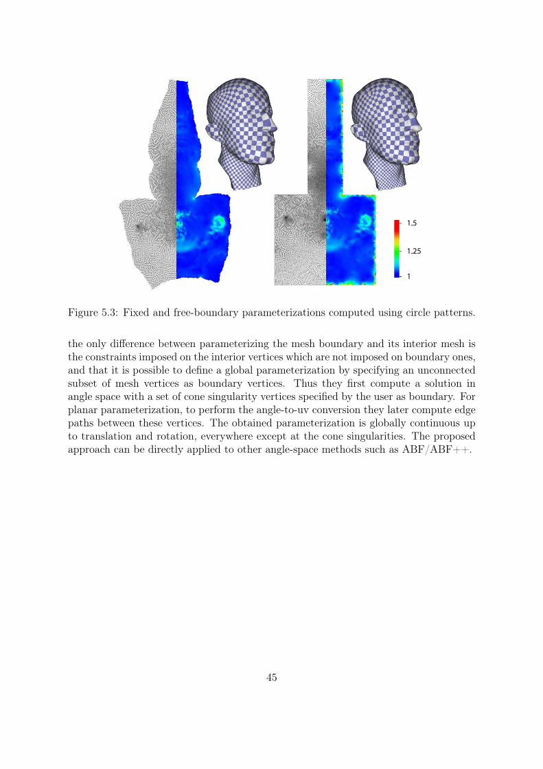
Figure 5.3: Fixed and free-boundary parameterizations computed using circle patterns.

the only difference between parameterizing the mesh boundary and its interior mesh isthe constraints imposed on the interior vertices which are not imposed on boundary ones,and that it is possible to define a global parameterization by specifying an unconnectedsubset of mesh vertices as boundary vertices. Thus they first compute a solution inangle space with a set of cone singularity vertices specified by the user as boundary. Forplanar parameterization, to perform the angle-to-uv conversion they later compute edgepaths between these vertices. The obtained parameterization is globally continuous upto translation and rotation, everywhere except at the cone singularities. The proposedapproach can be directly applied to other angle-space methods such as ABF/ABF++.

45

Figure 5.4: Global parameterization with cone singularities.

46

Chapter 6

Segmentation and Constraints1

For practical purposes planar mesh parameterization has to address two additional chal-lenges: segmenting closed or high genus meshes to enable planar embedding and enforc-ing specific point-to-point correspondences during parameterization.

6.1 Segmentation

Planar parameterization is only applicable to surfaces with disk topology. Hence, closedsurfaces and surfaces with genus greater than zero have to be cut prior to planar pa-rameterization. As previously noted, greater surface complexity usually increases para-meterization distortion, independent of the parameterization technique used. To allowparameterizations with low distortion, the surfaces must be cut to reduce the complexity.Since cuts introduce discontinuities into the parameterization, a delicate balance betweenthe conflicting goals of small distortion and short cuts has to be achieved. It is possibleto use constrained parameterization techniques to reduce cross-cut discontinuities.

Cutting and chart generation are most commonly used when computing parame-terizations for mapping of textures and other signals onto the surface. They are alsoused for applications such as compression and remeshing. The techniques for cuttingsurfaces can be roughly divided into two categories: segmentation techniques which par-tition the surface into multiple charts (Section 6.1.1), and seam generation techniqueswhich introduce cuts into the surface but keep it as a single chart (Section 6). Multiplecharts created by segmentation typically have longer boundaries than those created byseam cutting. However, they can often be more efficiently packed into a compact planardomain.

6.1.1 Multi-Chart Segmentations

Depending on the application, mesh segmentation techniques use different criteria forcreating charts. For parameterization, surfaces are broken into several charts such thatthe parametric distortion when parameterizing each chart is sufficiently low, while thenumber of charts remains small and their boundaries are kept as short as possible. Since

1This chapter is taken from [Sheffer et al., 2006] with minor changes.

47

Figure 6.1: Multi-chart segmentations (a) Isocharts [Zhou et al., 2004] – 13 charts; (b)[Lévy et al., 2002] – 44 charts; (c) D-charts [Julius et al., 2005] – 12 charts; (d) multi-chart geometry images [Sander et al., 2003] – 15 charts; and (e) [Zhang et al., 2005] –24 charts.

48

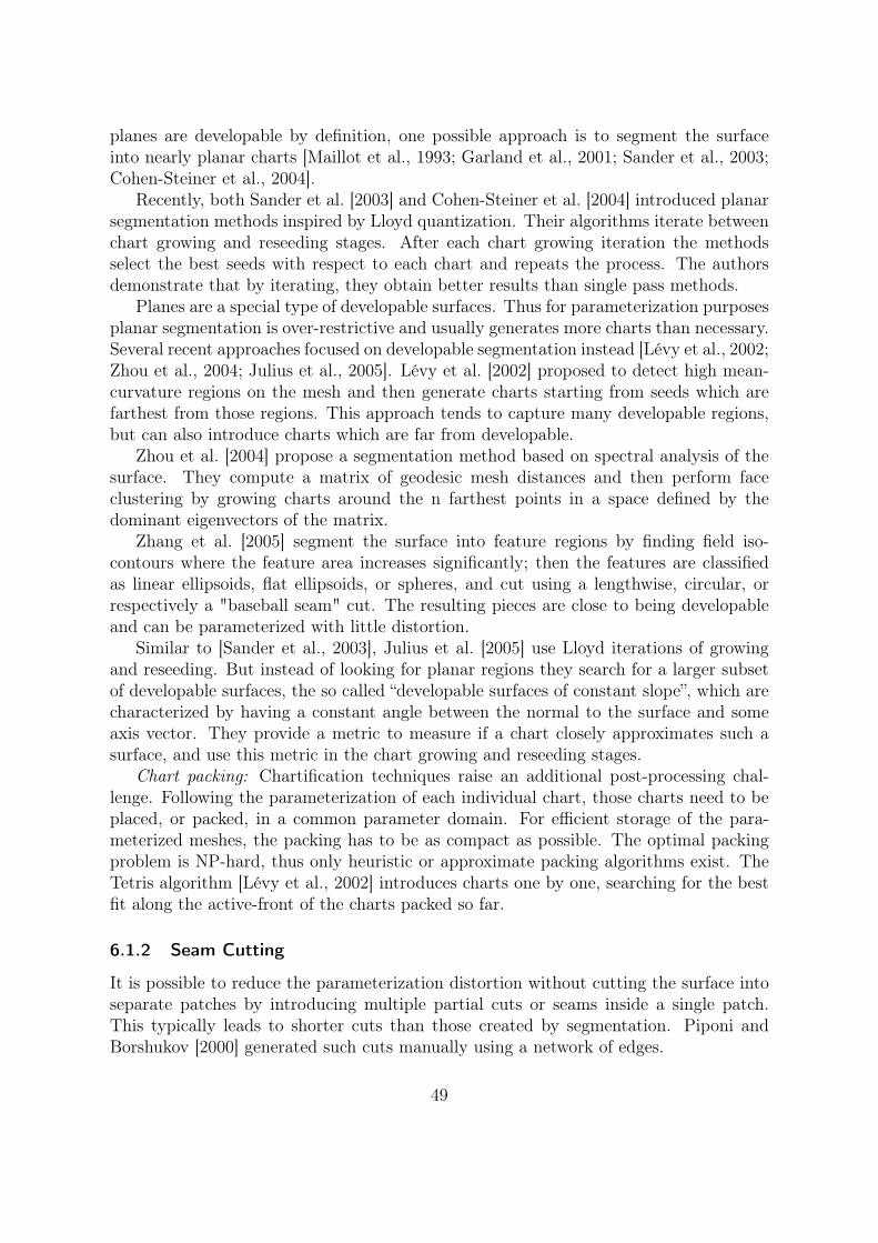
planes are developable by definition, one possible approach is to segment the surfaceinto nearly planar charts [Maillot et al., 1993; Garland et al., 2001; Sander et al., 2003;Cohen-Steiner et al., 2004].

Recently, both Sander et al. [2003] and Cohen-Steiner et al. [2004] introduced planarsegmentation methods inspired by Lloyd quantization. Their algorithms iterate betweenchart growing and reseeding stages. After each chart growing iteration the methodsselect the best seeds with respect to each chart and repeats the process. The authorsdemonstrate that by iterating, they obtain better results than single pass methods.

Planes are a special type of developable surfaces. Thus for parameterization purposesplanar segmentation is over-restrictive and usually generates more charts than necessary.Several recent approaches focused on developable segmentation instead [Lévy et al., 2002;Zhou et al., 2004; Julius et al., 2005]. Lévy et al. [2002] proposed to detect high mean-curvature regions on the mesh and then generate charts starting from seeds which arefarthest from those regions. This approach tends to capture many developable regions,but can also introduce charts which are far from developable.

Zhou et al. [2004] propose a segmentation method based on spectral analysis of thesurface. They compute a matrix of geodesic mesh distances and then perform faceclustering by growing charts around the n farthest points in a space defined by thedominant eigenvectors of the matrix.

Zhang et al. [2005] segment the surface into feature regions by finding field iso-contours where the feature area increases significantly; then the features are classifiedas linear ellipsoids, flat ellipsoids, or spheres, and cut using a lengthwise, circular, orrespectively a "baseball seam" cut. The resulting pieces are close to being developableand can be parameterized with little distortion.

Similar to [Sander et al., 2003], Julius et al. [2005] use Lloyd iterations of growingand reseeding. But instead of looking for planar regions they search for a larger subsetof developable surfaces, the so called “developable surfaces of constant slope”, which arecharacterized by having a constant angle between the normal to the surface and someaxis vector. They provide a metric to measure if a chart closely approximates such asurface, and use this metric in the chart growing and reseeding stages.

Chart packing: Chartification techniques raise an additional post-processing chal-lenge. Following the parameterization of each individual chart, those charts need to beplaced, or packed, in a common parameter domain. For efficient storage of the para-meterized meshes, the packing has to be as compact as possible. The optimal packingproblem is NP-hard, thus only heuristic or approximate packing algorithms exist. TheTetris algorithm [Lévy et al., 2002] introduces charts one by one, searching for the bestfit along the active-front of the charts packed so far.

6.1.2 Seam Cutting

It is possible to reduce the parameterization distortion without cutting the surface intoseparate patches by introducing multiple partial cuts or seams inside a single patch.This typically leads to shorter cuts than those created by segmentation. Piponi andBorshukov [2000] generated such cuts manually using a network of edges.

49

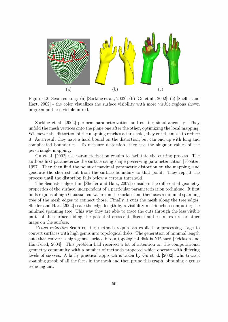
(a) (b) (c)

Figure 6.2: Seam cutting: (a) [Sorkine et al., 2002]; (b) [Gu et al., 2002]; (c) [Sheffer andHart, 2002] - the color visualizes the surface visibility with more visible regions shownin green and less visible in red.

Sorkine et al. [2002] perform parameterization and cutting simultaneously. Theyunfold the mesh vertices onto the plane one after the other, optimizing the local mapping.Whenever the distortion of the mapping reaches a threshold, they cut the mesh to reduceit. As a result they have a hard bound on the distortion, but can end up with long andcomplicated boundaries. To measure distortion, they use the singular values of theper-triangle mapping.

Gu et al. [2002] use parameterization results to facilitate the cutting process. Theauthors first parameterize the surface using shape preserving parameterization [Floater,1997]. They then find the point of maximal parametric distortion on the mapping, andgenerate the shortest cut from the surface boundary to that point. They repeat theprocess until the distortion falls below a certain threshold.

The Seamster algorithm [Sheffer and Hart, 2002] considers the differential geometryproperties of the surface, independent of a particular parameterization technique. It firstfinds regions of high Gaussian curvature on the surface and then uses a minimal spanningtree of the mesh edges to connect those. Finally it cuts the mesh along the tree edges.Sheffer and Hart [2002] scale the edge length by a visibility metric when computing theminimal spanning tree. This way they are able to trace the cuts through the less visibleparts of the surface hiding the potential cross-cut discontinuities in texture or othermaps on the surface.

Genus reduction Seam cutting methods require an explicit preprocessing stage toconvert surfaces with high genus into topological disks. The generation of minimal lengthcuts that convert a high genus surface into a topological disk is NP-hard [Erickson andHar-Peled, 2004]. This problem had received a lot of attention on the computationalgeometry community with a number of methods proposed which operate with differinglevels of success. A fairly practical approach is taken by Gu et al. [2002], who trace aspanning graph of all the faces in the mesh and then prune this graph, obtaining a genusreducing cut.

50

(a) (b) (c)

Figure 6.3: Constraint enforcement with Matchmaker [Kraevoy et al., 2003]: (a) Texture(two photos) with feature points specified; (b) input model with corresponding verticeshighlighted; (c) resulting texture.

(a) (b) (c)

Figure 6.4: Combining multiple textures [Zhou et al., 2005].

Figure 6.5: Two examples of constrained texture mapping [Lévy, 2001]

51

6.2 Constraints

Sometimes a parameterization needs to accommodate user constraints, specifying corre-spondences between vertices of the mesh. The most important application of constrainedparameterization is texture mapping 3D models from photographs [Lévy, 2001; Kraevoyet al., 2003] (see Figures 6.5 and 6.3). Zhou et al. [2005] use more complex constraints toallow the user to combine several images to produce a complete texture for a mesh. Con-strained parameterization can also be used to hide cross-seam discontinuities [Kraevoyet al., 2003; Zhou et al., 2005].

The methods for enforcing constraints can be split into two types, those that enforcesoft or approximate constraints and that that enforce hard constraints. Methods basedon energy minimization can accommodate soft constraints by adding a quadratic termto the energy function, measuring the distance between the constraint features in thecurrent configuration and their desired location [Lévy, 2001]. Such constraints workreasonably well in practice, and can be solved efficiently, since they only add linearterms to the energy, but sometimes break theoretical guarantees about the originalparameterization method, such as bijectivity. The degree of constraint approximationtypically decreases with the distance between the constrained and unconstrained vertexlocations. Some applications, such as hiding texture discontinuities along seams in theparameterization [Kraevoy et al., 2003; Zhou et al., 2005] require hard constraints toachieve perfect alignment of the texture along the seams.

One way to enforce hard constraints is by adding them into a regular parameteriza-tion formulation using Lagrange multipliers [Desbrun et al., 2002]. This approach allowsconstraints to be defined on points inside triangles and on arbitrary line segments (thevertices of the triangulation can be constrained more easily by taking the correspondingvariables out of the system). However, it is easy to show that for a given mesh connec-tivity not every set of constraints can be satisfied. Thus methods like this that preservethe mesh connectivity will fail to generate bijective parameterizations for many inputs.

Methods that enforce hard-constraints robustly, introduce additional vertices intothe mesh as they go along to ensure that a constrained solution exists. Eckstein et al.[2001] enforce hard constraints by deforming an existing embedding while adding newvertices when necessary. Theoretically, this method can handle large sets of constraintsbut is extremely complicated.

The Matchmaker algorithm [Kraevoy et al., 2003] compute the parameterization byestablishing coarse patch correspondences between the input and the parameter do-main. The provided feature points on the input model and the parameter domain areconnected using a network of curves that partition the surface into patches that arethen parameterized while trying to maintain continuity and smoothness between them.The curve tracing process is guided by a set of topological rules that ensure that theresulting patches will be consistent between the objects being parameterized and thedomain. They compute the triangulations of the input and the parameter domain si-multaneously. Continuity and smoothness between patches can be obtained by relaxingthe parameterization.

Zhou et al. [2005] allow the user to combine several images to produce texture for a

52

mesh, by assigning some surface patches to different images, as well as using in-paintingtechniques to create texture for any unassigned transition patches between them. Inaddition to geometric smoothness of the map, they take into account the continuityof the texture signal being applied since it may come from different sources for twoneighboring patches.

53

Chapter 7

Comparison of Planar Methods

The different methods reviewed minimize different types of distortion metrics. Ide-ally, most parameterization applications work best on zero distortion parameterizations,though most are tolerant to some amount of distortion, some being more tolerant toshear and others to stretch. In general, applications that depend on regular grids forsampling, such as different types of detail mapping and synthesis, as well as compressionand regular resampling schemes (e.g. geometry images [Gu et al., 2002]), tend to per-form better on stretch minimizing parameterizations, since stretch is directly related tounder-sampling. In contrast, applications based on irregular sampling, such as remesh-ing [Desbrun et al., 2002], are very sensitive to shearing, but can handle quite significantstretch. When acceptable levels of shear or stretch are not attainable because a surfaceis too complex, the surface needs to be cut prior to parameterization in order to achieveacceptable distortion.

In addition to distortion, several other factors should be considered when choosing aparameterization method for an application at hand:

• Free versus fixed boundary. Many methods assume the boundary of the planardomain is pre-defined and convex. Fixed boundary methods typically use verysimple formulations and are very fast. Such methods are well suited for someapplications, for instance those that utilize a base mesh parameterization, seeSection 5.1. Free-boundary techniques, which determine the boundary as part ofthe solution, are often slower, but typically introduce significantly less distortion.

• Robustness. Most applications of parameterization require it to be bijective. Forsome applications local bijectivity (no triangle flips) is sufficient while others re-quire global bijectivity conditions (the boundary does not self-intersect). Only asubset of the parameterization methods can guarantee local or global bijectivity.Some of the others can guarantee bijectivity if the input meshes satisfy specificconditions.

• Numerical Complexity. The existing methods can be roughly classified accordingto the optimization mechanism they use into linear and non-linear methods. Linearmethods are typically significantly faster and simpler to implement. However, asexpected the simplicity usually comes at the cost of increased distortion.

54

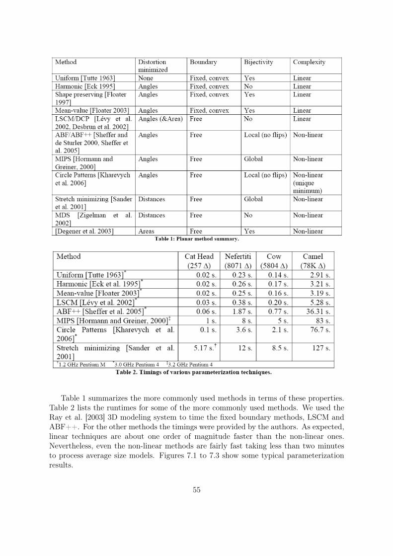
Table 1 summarizes the more commonly used methods in terms of these properties.Table 2 lists the runtimes for some of the more commonly used methods. We used theRay et al. [2003] 3D modeling system to time the fixed boundary methods, LSCM andABF++. For the other methods the timings were provided by the authors. As expected,linear techniques are about one order of magnitude faster than the non-linear ones.Nevertheless, even the non-linear methods are fairly fast taking less than two minutesto process average size models. Figures 7.1 to 7.3 show some typical parameterizationresults.

55

Figure 7.1: Surfaces with nearly convex boundaries parameterized with linear methods(images made with Graphite, http://alice.loria.fr/software).

56

Figure 7.2: Surfaces with non-convex boundaries parameterized with linear methods(images made with Graphite, http://alice.loria.fr/software).

57

Figure 7.3: Surfaces with non-convex boundaries parameterized with non-linear methods(images made with Graphite, http://alice.loria.fr/software).

58

Chapter 8

Alternate base domains

Some applications are quite sensitive to discontinuities in the parameterization, or cannottolerate them at all. In such cases, when the object to be parameterized is not a topo-logical disc, it is worthwhile to use a different base domain for the parameterization.Examples of such domains that have been investigated include simplicial complexes,spheres, and periodic planar regions with transition curves.

In addition, numerous applications of parameterization require cross-parameteriza-tion or intersurface mapping between multiple models. Pair-wise mapping between mod-els can be used for the transfer of different properties between the models, includingstraightforward ones, such as texture, and less obvious ones such as deformation andanimation. It can also be used for blending and morphing, as well as mesh completionand repair. The most common approach for pair-wise mapping is to parameterize bothmodels on a common base domain. Free-boundary planar parameterization is clearlyunsuitable for this purpose. Instead alternate domains such as a simplicial complex ora sphere are commonly used.

8.1 The Unit Sphere

The big advantage of the spherical domain over the planar one is that it allows forseamless, continuous parameterization of genus-0 models, and there are a large numberof such models in use. Thus, the spherical domain has received much attention in thelast few years, with several papers published about this topic. Some rigorous theory isbeing developed, getting close to the level of understanding we have of planar parame-terizations. These notes cover four main types of spherical parameterization approaches:Gauss-Seidel iterative extension of planar barycentric methods; stereographic projection;spherical generalization of barycentric coordinates; and multi-resolution embedding.

One attractive approach for spherical parameterization is to extend the barycentric,convex boundary planar methods to the sphere. Several methods [Alexa, 2000; Gu andYau, 2002; Kobbelt et al., 1999] used Gauss-Seidel iterations to obtain such parameteri-zation. They start by computing an initial guess and then moving the vertices one at atime, first computing a 3D position for the vertex using a barycentric formulation [Ecket al., 1995], and then projecting the vertex to the unit sphere. Isenburg et al. [2001]

59

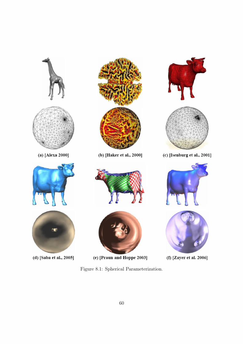
Figure 8.1: Spherical Parameterization.

60

split the mesh in two, map the cut onto a great circle and embed each half-mesh ontoa hemisphere using a modified Tutte procedure. Regrettably, as proven by Saba et al.[2005] projected Gauss-Seidel iterations decrease the residual for only a finite number ofiterations. As the result approaches a bijective solution, the scheme ultimately becomesunstable, the residual increases, and the system collapses to a degenerate solution. Sabaet al. [2005] note that this behaviour is independent of step size.

Haker et al. [2000] compute a planar parameterization of the mesh first, using oneof the triangles as a boundary. They then use the stereographic projection to obtainthe spherical mapping. The result depends quite heavily on the choice of the boundarytriangle. This approach works quite well in practice, however it doesn’t offer any theo-retical guarantees since the stereographic projection is bijective only for the continuouscase, and can produce triangle flips in the discrete case. A simple proof by example ofthis statement can be obtained by imagining the great circle supporting the edge ABof a mapped spherical triangle ABC. The (continuous) stereographic projection mapsthis great circle to a circle in the original plane. The third vertex C can be perturbedin the plane to cross from the interior to the exterior of the circle, without changingthe triangle orientation. The spherical triangle ABC will flip however as a result of thisperturbation, as the image of C on the sphere will cross from one side to the other ofthe spherical edge AB.

Gotsman et al. [2003] showed how to correctly generalize the method of barycentriccoordinates, with all its advantages, to the sphere. The generalization is based on resultsfrom spectral graph theory due to de Verdière [1993] and extensions due to Lovász andSchrijver [1999]. They provide a quadratic system of equations which is a sphericalequivalent of the barycentric formulation. The authors do not provide an efficient wayto solve the resulting system, and thus their method is limited to very small meshes.Saba et al. [2005] introduce a method for efficiently solving the system, by providinga good initial guess and using a robust solver. First, similar to [Isenburg et al., 2001],they partition the mesh in two, and embed each half on a hemisphere using a planarparameterization followed by a stereographic projection. They then use a numericalsolution mechanism which combines Gauss-Seidel iteration with nonlinear minimizationto obtain the final solution.

An efficient and bijective alternative is suggested by multi-resolution techniques.These methods obtain an initial guess by simplifying the model until it becomes a tetra-hedron (or at least, convex), trivially embed it on the sphere, and then progressivelyadd back the vertices [Shapiro and Tal, 1998; Praun and Hoppe, 2003]. Shapiro and Tal[1998] compute the embedding using purely topological operations and do not attempt tominimize any type of distortion. Praun and Hoppe [2003] obtain a spherical parameteri-zation by alternating refining steps that add vertices from a multi-resolution decomposi-tion of the object with relaxation of single vertex locations inside their neighbourhoods.The relaxation is aimed to minimize the stretch metric of the parameterization and isguaranteed to maintain a valid embedding.

61

Figure 8.2: A,B: Parameterization methods for disk-topology combined with segmenta-tion algorithms can create a texture atlas from a shape of arbitrary topology. However,the large number of discontinuities can be problematic for the applications. C: Globalparameterization algorithms do not suffer from this problem. (Data courtesy of the DigitalMichelangelo Project, Stanford).

8.2 Simplicial and quadrilateral complexes

As seen in Chapters 3 and 4, parameterization methods can put a 3D shape with disktopology in one-to-one correspondence with a 2D domain. For a shape with arbitrarytopology, it is possible to decompose the shape into a set of charts, using a segmentationalgorithm (e.g. VSA [Cohen-Steiner et al., 2004]). Each chart is then parameterized (seeFigure 8.2-A,B). Even if this solution works, it is not completely satisfactory : why oneshould “damage” the surface just to define a coordinate system on it ? From the appli-cation point of view, chart boundaries are difficult to handle in remeshing algorithms,and introduce artefacts in texture mapping applications. For this reason, we focus inthis section on global parameterization algorithms, that do not require segmenting thesurface. (Figure 8.2-C).

To compute such a global parameterization, the geometry processing community firstdeveloped methods that operate by segmenting / prameterizing / and resampling theobject. To our knowledge, this idea was first developed in the MAPS method [Lee et al.,1998] (Multiresolution Adaptive Parameterization of Surfaces). As shown in Figure 8.3,this method starts by partitioning the initial object (Figure 8.3-A) into a set of trian-gular charts, called the base complex (Figure 8.3-C). Then, a parameterization of eachchart is computed, and the object is regularly resampled in parametric space (Figure8.3-C). Further refinements of the method improved the inter-chart continuity [Kho-

62

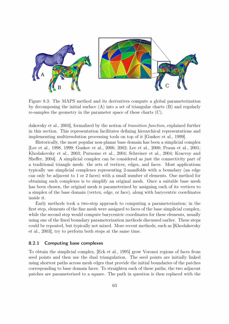
Figure 8.3: The MAPS method and its derivatives compute a global parameterizationby decomposing the initial surface (A) into a set of triangular charts (B) and regularlyre-samples the geometry in the parameter space of these charts (C).

dakovsky et al., 2003], formalized by the notion of transition function, explained furtherin this section. This representation facilitates defining hierarchical representations andimplementing multiresolution processing tools on top of it [Guskov et al., 1999].

Historically, the most popular non-planar base domain has been a simplicial complex[Lee et al., 1998, 1999; Guskov et al., 2000, 2002; Lee et al., 2000; Praun et al., 2001;Khodakovsky et al., 2003; Purnomo et al., 2004; Schreiner et al., 2004; Kraevoy andSheffer, 2004]. A simplicial complex can be considered as just the connectivity part ofa traditional triangle mesh: the sets of vertices, edges, and faces. Most applicationstypically use simplicial complexes representing 2-manifolds with a boundary (an edgecan only be adjacent to 1 or 2 faces) with a small number of elements. One method forobtaining such complexes is to simplify an original mesh. Once a suitable base meshhas been chosen, the original mesh is parameterized by assigning each of its vertices toa simplex of the base domain (vertex, edge, or face), along with barycentric coordinatesinside it.

Early methods took a two-step approach to computing a parameterization; in thefirst step, elements of the fine mesh were assigned to faces of the base simplicial complex,while the second step would compute barycentric coordinates for these elements, usuallyusing one of the fixed boundary parameterization methods discussed earlier. These stepscould be repeated, but typically not mixed. More recent methods, such as [Khodakovskyet al., 2003], try to perform both steps at the same time.

8.2.1 Computing base complexes

To obtain the simplicial complex, [Eck et al., 1995] grow Voronoi regions of faces fromseed points and then use the dual triangulation. The seed points are initially linkedusing shortest paths across mesh edges that provide the initial boundaries of the patchescorresponding to base domain faces. To straighten each of these paths, the two adjacentpatches are parameterized to a square. The path in question is then replaced with the

63

diagonal of the square mapped onto the mesh surface.[Lee et al., 1998] simplify the original mesh, keeping track of correspondences between

the original vertices and the faces of the simplified mesh. Others, like [Guskov et al.,2000] (Figure 13 (c)) and [Khodakovsky et al., 2003] use clustering techniques to generatethe patch connectivity and derive the base-mesh from it.

The construction becomes more challenging when multiple models need to be pa-rameterized on the same complex [Praun et al., 2001; Schreiner et al., 2004; Kraevoyand Sheffer, 2004]. Praun et al. [2001] partition a mesh into triangular patches, whichcorrespond to the faces of a user given simplicial complex, by drawing a network of pathsbetween user-supplied feature vertices that correspond to the vertices of the base mesh.

Schreiner et al. [2004] and Kraevoy and Sheffer [2004] extend the methods of Praunet al. [2001] and Kraevoy et al. [2003] to construct the simplicial complex automatically,in parallel to the patch formation. The input to both methods includes a set of corre-spondences between feature vertices on the two input models. The methods use those asthe vertices of the base complex. They simultaneously trace paths on the input meshesbetween corresponding pairs of vertices, splitting existing mesh edges if necessary. Tariniet al. [2004] were the first, to our knowledge, to use a quadrilateral base domain. Sucha domain is much more suitable for quadrilateral remeshing of the input surface and forspline fitting. Tarini et al. [2004] generate the base domain manually.

8.2.2 Mapping to the base mesh

Once the discrete assignment to base domain faces has been done, the barycentric coordi-nates can be computed using fixed-boundary planar parameterization. Earlier methodscomputed the barycentric coordinates once, based on the initial assignment of the ver-tices to the base triangles. More recent methods [Khodakovsky et al., 2003; Kraevoyand Sheffer, 2004, 2005; Tarini et al., 2004] use an iterative process where vertices canbe reassigned between base faces.

Khodakovsky et al. [2003] perform the vertex-to-patch assignment and coordinate re-laxation in a single procedure, by letting vertices cross patch boundaries using transitionfunctions. A transition function expresses the barycentric coordinates of a vertex withrespect to a base domain face as barycentric coordinates for a neighboring base domainface. For this procedure only the images of the base domain vertices needs to be fixed,rather than the edges as well as in the previous methods. The authors relax the basedomain vertices separately, prompting a new run of the main relaxation. In practice, thiscycle is repeated only very few times. The implementation sometimes needs to discardsome relaxation results when mesh vertices moved around base domain vertices end upwith barycentric coordinates that are invalid for all the base domain faces around thatvertex.

Tarini et al. [2004] and Kraevoy and Sheffer [2004, 2005] fix the boundary of a groupof base mesh faces, update the barycentric coordinates in the interior, and then possiblyre-assign some vertices to different faces inside the group. The methods differ in thegrouping they use and the choice of parameterization technique used for the barycentriccoordinates computation.

64

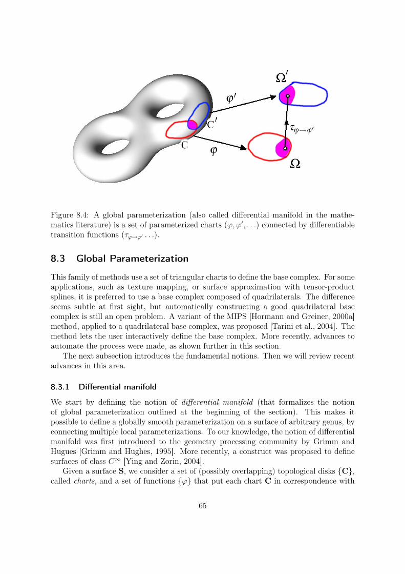
Figure 8.4: A global parameterization (also called differential manifold in the mathe-matics literature) is a set of parameterized charts (ϕ, ϕ′, . . .) connected by differentiabletransition functions (τϕ→ϕ′ . . .).

8.3 Global Parameterization

This family of methods use a set of triangular charts to define the base complex. For someapplications, such as texture mapping, or surface approximation with tensor-productsplines, it is preferred to use a base complex composed of quadrilaterals. The differenceseems subtle at first sight, but automatically constructing a good quadrilateral basecomplex is still an open problem. A variant of the MIPS [Hormann and Greiner, 2000a]method, applied to a quadrilateral base complex, was proposed [Tarini et al., 2004]. Themethod lets the user interactively define the base complex. More recently, advances toautomate the process were made, as shown further in this section.

The next subsection introduces the fundamental notions. Then we will review recentadvances in this area.

8.3.1 Differential manifold

We start by defining the notion of differential manifold (that formalizes the notionof global parameterization outlined at the beginning of the section). This makes itpossible to define a globally smooth parameterization on a surface of arbitrary genus, byconnecting multiple local parameterizations. To our knowledge, the notion of differentialmanifold was first introduced to the geometry processing community by Grimm andHugues [Grimm and Hughes, 1995]. More recently, a construct was proposed to definesurfaces of class C∞ [Ying and Zorin, 2004].

Given a surface S, we consider a set of (possibly overlapping) topological disks C,called charts, and a set of functions ϕ that put each chart C in correspondence with

65

a 2D domain Ω (c.f. Figure 8.4). The 2D coordinates will be denoted by θ, φ. The setof functions ϕ defines a differential manifold if the following condition is satisfied :Given two charts C and C′, if their intersection C∩C′ is homeomorphic to a disk, thenthe two images of their intersection C ∩ C′ in parametric space through ϕ and ϕ′ arelinked by a differentiable geometric transform τϕ→ϕ′:

∀p ∈ C ∩C′, ϕ′(p) = τϕ→ϕ′ (ϕ(p))

The functions τϕ→ϕ′ are called transition functions [Khodakovsky et al., 2003]). Amanifold is said to be affine if all the transition functions are translations. Complexmanifolds admit any one-to-one conformal function as a transition function (c.f. Sec-tion 4.3 for the notion of conformality). In particular, this includes similarities, i.e.functions composed of translations, rotations and scalings.

8.3.2 Exterior calculus

By using a representation of a manifold as a set of charts (with the associated transitionfunctions), it is possible to manipulate functions defined over the manifold, compute theirgradients and integrate them over subsets of the manifold. However, these computationsoften involve the Jacobian matrix of each local parameterization in a non-trivial manner,and make all the computations quite involved. Despite the possibility of using formaltools (e.g. Maple), this way of conducting computations remains frustrating from anintellectual point of view.

Exterior calculus is an elegant alternative to this problem. This is a geometric calcu-lus, without coordinates, that considers the functions as abstract mathematical objects,combined with operators. At the end, to use the functions, one still needs to “instantiate”them in a local coordinate frame. However, by post-poning the (lower-level) represen-tation in coordinates at the end of the mathematical reasoning, most computations aresimplified by higher level considerations, guided by the algebraic structure defined bythe functions and the operators.

Exterior calculus generalizes the fundamental theorem of calculus, that defines theintegral of a function : ∫ b

a

f(x)dx = F (b)− F (a)

where F denotes the primitive of f .The generalized theorem writes: ∫

Ω

dω =

∫∂Ω

ω

where ω is a differential k-form, ∂Ω denotes the border of Ω, and d denotes the exteriorderivative. For the moment, one may think about a k-form as something that wantsto be integrated over a k-dimensional domain. Therefore, 0-forms correspond to classicfunctions, 1-form to vector fields (that one can integrate along a curve), and 2-formsto functions that one wants to integrate over a surfacic domain. About the exterior

66

derivative, this is a generalization of the gradient operator. The exterior derivative hasalso the noticeable property of vanishing when applied twice (ddω = 0), we will explainwhy further.

The divergence theorem (Ostrogradsky-Gauss) is a particular case :∫vol

divKdv =

∫∂vol

K ·NdS

where N denotes the normal to the border of the volume. Note that in the “exteriorcalculus” version, the scalar product with the normal is already taken into account by theintegration over ∂Ω (this is the way exterior calculus considers the border of a subset).More generally, exterior calculus exhibits a symmetry between the integrated entities(called differential forms) and the integration domains (called chains). The integrationof a form ω over a chain Ω is then a certain type of inner product (or dot product)< ω, Ω >. The border operator ∂ computes the border ∂Ω of a chain Ω, and returnsanother chain, of lower dimension. With this notation, Stokes theorem writes :

< dω, Ω >=< ω, ∂Ω >

in other words, from an intuitive point of view, the exterior derivative d becomes theborder operator ∂ when one “shifts” if from the integrated form ω to the integrationdomain Ω. This exhibits the duality between the exterior derivative d and the borderoperator ∂. For this reason, differential forms are also called co-chains and the exteriorderivative is also called the co-border operator1.

Finally, one can note that the fundamental theorem of calculus is retrieved as aspecial case : ∫

(a,b)

f(x)dx =

∫a,b

dF =

∫a−∪b+

F = F (b)− F (a)

This is the orientation of the border ∂(a, b) = a− ∪ b+ that introduces the “-” sign infront of F (a).

To our knowledge, notions of exterior calculus first appeared in the community inPinkall and Polthier’s paper [Pinkall and Polthier, 1993], where they used Hodge dualityto compute minimal surfaces. Then, Gu et. al [Gu and Yau, 2003; Jin et al., 2004] usedthe fundamental notions involved in Poincaré’s conjecture to compute global parame-terizations. Anil Hirani developed in his Ph.D thesis a discrete counterpart of exteriorcalculus (DEC) [Hirani, 2003], especially well suited to geometry processing with meshes.More recently, in 2005, Schröeder and Desbrun gave a course at SIGGRAPH about DEC.This latter course contributed to make these complex abstract notions accessible to awider community, and we redirect the interested reader to their course notes for moredetails on this fascinating topic. The next subsection quickly reviews methods based onco-homology (and introduces the related notions). In what follows, we keep the generalcontinuous setting for the explanations.

67

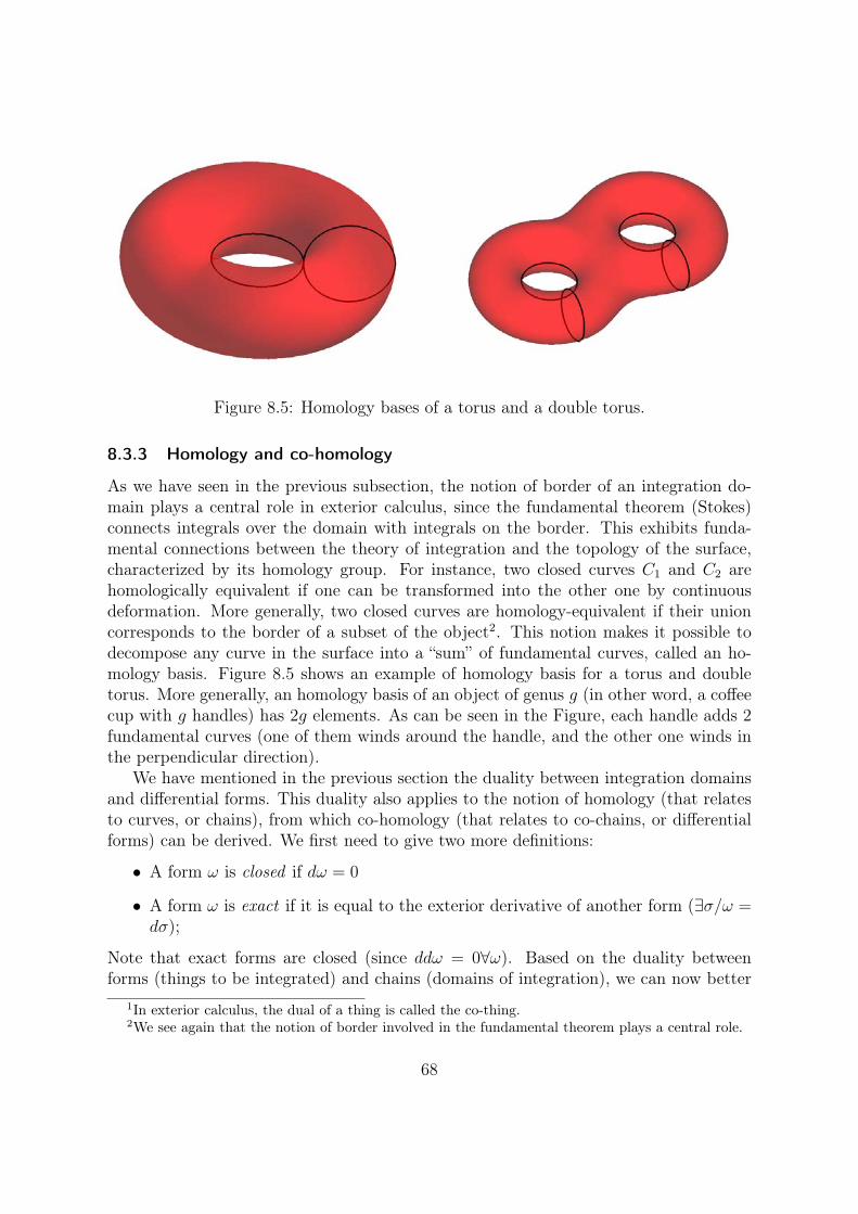
Figure 8.5: Homology bases of a torus and a double torus.

8.3.3 Homology and co-homology

As we have seen in the previous subsection, the notion of border of an integration do-main plays a central role in exterior calculus, since the fundamental theorem (Stokes)connects integrals over the domain with integrals on the border. This exhibits funda-mental connections between the theory of integration and the topology of the surface,characterized by its homology group. For instance, two closed curves C1 and C2 arehomologically equivalent if one can be transformed into the other one by continuousdeformation. More generally, two closed curves are homology-equivalent if their unioncorresponds to the border of a subset of the object2. This notion makes it possible todecompose any curve in the surface into a “sum” of fundamental curves, called an ho-mology basis. Figure 8.5 shows an example of homology basis for a torus and doubletorus. More generally, an homology basis of an object of genus g (in other word, a coffeecup with g handles) has 2g elements. As can be seen in the Figure, each handle adds 2fundamental curves (one of them winds around the handle, and the other one winds inthe perpendicular direction).

We have mentioned in the previous section the duality between integration domainsand differential forms. This duality also applies to the notion of homology (that relatesto curves, or chains), from which co-homology (that relates to co-chains, or differentialforms) can be derived. We first need to give two more definitions:

• A form ω is closed if dω = 0

• A form ω is exact if it is equal to the exterior derivative of another form (∃σ/ω =dσ);

Note that exact forms are closed (since ddω = 0∀ω). Based on the duality betweenforms (things to be integrated) and chains (domains of integration), we can now better

1In exterior calculus, the dual of a thing is called the co-thing.2We see again that the notion of border involved in the fundamental theorem plays a central role.

68

understand the terminology and notations : the boundary operator ∂ is dual to theexterior derivative d, a closed form ω (i.e. such that dω = 0) is dual to a closed chain Ω(i.e. such that ∂Ω = 0). Moreover, the boundary of a chain is always closed (∂∂Ω = ),this explains why the exterior derivative vanishes when applied twice (ddω = 0).

We can now elaborate on co-homology : on a surface, one can associate to eachfundamental curve of the homology basis a set of closed 1-forms (e.g. vector fields) thatare equivalent with respect to co-homology. More precisely, two 1-forms ω1 and ω2 areequivalent if their integral along all the curves of the homology basis match. Note thatthis is the case if their difference ω2 − ω1 is exact since the integration of the differencealong an element Ω of the homology basis gives :

∃σ/ω2 − ω1 = dσ ⇒< Ω, dσ >=< ∂Ω, σ >=< , σ >= 0

(we remind that the elements of the homology basis are closed curves). We can nowgive the general definition of co-homology, that is to say the quotient space of closedforms on exact forms (i.e. two closed forms are equivalent if their difference is an exactform). This relation is dual to homology: two closed curves are equivalent if they arethe border of a subset3.

As shown in Figure 8.6, Gu and Yau used these notions to compute a global con-formal parameterization on a surface of arbitrary genus [Gu and Yau, 2003; Jin et al.,2004]. To do so, they compute a holomorphic function (i.e. the generalization of con-formal functions mentioned in Section 4.3), based on an important theorem that statesthat each co-homology class contains a unique harmonic one-form. We have alreadyseen that the coordinates of a conformal map are two harmonic functions. Similarly,a holomorphic function is composed of two conjugate (i.e. orthogonal) harmonic one-forms. Then, their method operates as follows : they first compute a homology basisof the surface (using for instance Erickson’s method [Erickson and Whittlesey, 2005] orLazarus’s one [Lazarus et al., 2001]) (A), then they deduce a co-homology basis, andfind a pair of conjugate harmonic one-forms (B). Finally, they integrate the one-forms tofind the parameterization (C). Note that for an object of genus g, the parameterizationhas necessarily 2g singularities. Ray et.al [Ray et al., 2006] have proposed a way of au-tomating the placement of these singularities and generalize them to fractional indices(see Figure 8.7).

In practice, the discrete version of Gu et. al ’s framework operates by solving linearsystems with three types of constraints: harmonicity, closedness, and duality. Theharmonicity equations are similar to the ones used by planar methods: the sum ofvectors for edges incident to a vertex, weighed by the cotangent harmonic weights, iszero. The closedness equations state that the sum of the 3 vectors for the edges of eachface is zero (a “gradient field” has no divergence). The duality conditions replace theboundary conditions in traditional parameterizations; they impose fixed values for theintegral of the field on the closed loops forming the homology basis of the surface (the 2gcurves that cut open the handles of the mesh, where g is the genus of the surface). Several

3Being the border of a subset is dual to exactness for forms.

69

Figure 8.6: The method developed by Gu and Yau to construct a differential manifoldfirst computes a homology basis (A), then deduces a co-homology basis and finds the(unique) harmonic one form in each co-homology class (B). Finally, the u and v poten-tials are obtained by integrating these harmonic one-forms (C), that together define aholomorphic function (D) (data courtesy of Stanford, parameterization courtesy of X. Gu)

70

Figure 8.7: It is well known from mathematicians and rattan objects makers that themesh of an object of genus g has 2g singularities (or poles). Thus, a sphere (g = 1)has two poles (A). It is possible to subdivide a pole into two half-poles (B) or fourquarter-poles (C). The order of multiplicity of a pole, or the rotation angle that themesh undergoes when turning around the pole is called the index of the pole.

systems are solved, in each system the integral across one of the curves is constrainedto 1, and all the others to 0.

Other authors have proposed methods that directly compute the parameterization,based on modified Floater conditions. For instance, Steiner and Fischer have proposed tomake the object equivalent to a disk using a cut graph, and insert translation vectors inTutte’s conditions related to the vertices located on the cut graph [Steiner and Fischer,2005]. Tong et.al developed independently the same idea [Tong et al., 2006], using theformalism of exterior calculus mentioned above, and adding singularities of fractionalindex.

To summarize, these methods [Gu and Yau, 2002; Kharevych et al., 2006; Tong et al.,2006] implicitly create a parameterization by solving for differential one-forms. Insteadof associating (u, v) coordinates with vertices as in typical planar parameterization, theyassociate planar vectors (du, dv) with the edges of the mesh, computing a gradient field,or one-form. These parameterizations can be converted to a special form of planarparameterization by fixing a vertex, then walking around to other vertices and adding

71

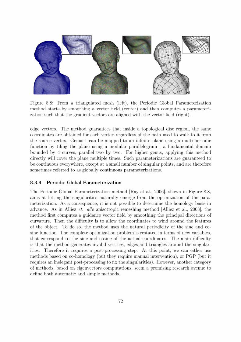
Figure 8.8: From a triangulated mesh (left), the Periodic Global Parameterizationmethod starts by smoothing a vector field (center) and then computes a parameteri-zation such that the gradient vectors are aligned with the vector field (right).

edge vectors. The method guarantees that inside a topological disc region, the samecoordinates are obtained for each vertex regardless of the path used to walk to it fromthe source vertex. Genus-1 can be mapped to an infinite plane using a multi-periodicfunction by tiling the plane using a modular parallelogram - a fundamental domainbounded by 4 curves, parallel two by two. For higher genus, applying this methoddirectly will cover the plane multiple times. Such parameterizations are guaranteed tobe continuous everywhere, except at a small number of singular points, and are thereforesometimes referred to as globally continuous parameterizations.

8.3.4 Periodic Global Parameterization

The Periodic Global Parameterization method [Ray et al., 2006], shown in Figure 8.8,aims at letting the singularities naturally emerge from the optimization of the para-meterization. As a consequence, it is not possible to determine the homology basis inadvance. As in Alliez et. al ’s anisotropic remeshing method [Alliez et al., 2003], themethod first computes a guidance vector field by smoothing the principal directions ofcurvature. Then the difficulty is to allow the coordinates to wind around the featuresof the object. To do so, the method uses the natural periodicity of the sine and co-sine function. The complete optimization problem is restated in terms of new variables,that correspond to the sine and cosine of the actual coordinates. The main difficultyis that the method generates invalid vertices, edges and triangles around the singular-ities. Therefore it requires a post-processing step. At this point, we can either usemethods based on co-homology (but they require manual intervention), or PGP (but itrequires an inelegant post-processing to fix the singularities). However, another categoryof methods, based on eigenvectors computations, seem a promising research avenue todefine both automatic and simple methods.

72

8.3.5 Spectral methods

Spectral methods study the eigenfunctions of operators (or eigenvectors of matricesin the discrete setting). Several reviews on this topic are available [Gotsman, 2003;Lévy, 2006], and we also give some web references on the following webpage http://alice.loria.fr/publications.

We focus on the Laplace operator, that plays a fundamental role in conformal meshparameterization, as shown in Section 4.3.

The eigenfunctions f of the Laplace operator ∆ are characterized by :

∆f = λf

Before elaborating on the eigenfunctions, we give more detailed about the Lapla-cian and its generalizations. The Laplacian plays a fundamental role in physics andmathematics. In R

n, it is defined as the divergence of the gradient:

∆ = div grad = ∇.∇ =∑

i

∂2

∂x2i

Intuitively, the Laplacian generalizes the second order derivative to higher dimensions,and is a characteristic of the irregularity of a function as ∆f(P ) measures the differencebetween f(P ) and its average in a small neighborhood of P . Generalizing the Lapla-cian to curved surfaces require complex calculations, that can be greatly simplified by amathematical tool called exterior calculus (EC). See section 8.3.2 or Peter Schroeder’sSiggraph 2005 course for more details about exterior calculus. EC generalizes the gra-dient by d and divergence by δ = ∗d∗ (where ∗ denotes the Hodge star), which are builtindependently of any coordinate frame. Using EC, the definition of the Laplacian canbe generalized to functions defined over a manifold S with metric g, and is then calledthe Laplace-Beltrami operator:

∆ = div grad = δd =∑

i

1√|g|

∂

∂xi

√|g| ∂

∂xi

where |g| denotes the determinant of g. The additional term√|g| can be interpreted as a

local "scale" factor since the local area element dA on S is given by dA =√|g|dx1∧dx2.

The eigenfunctions and eigenvalues of the Laplacian on a (manifold) surface S, areall the pairs (Hk, λk) that satisfy −∆Hk = λkH

k. The “−” sign is here required forthe eigenvalues to be positive. On a closed curve, the eigenfunctions of the Laplaceoperator define the function basis (sines and cosines) of Fourier analysis4. On a square,they correspond to the function basis of the DCT (Discrete Cosine Transform), usedfor instance by the JPEG image format. Finally, the eigenfunctions of the Laplace-Beltrami operator on a sphere define the Spherical Harmonics basis. Figure 8.9 showshow they look like for a more general object. Since it generalizes spherical harmonics

4This is easy to check by noticing that in 1D, the Laplace operator corresponds to the standard secondorder derivative. The eigenfunctions are simply sinωt (resp. cos) associated with the eigenvalues −ω2.

73

Figure 8.9: Some of the eigenfunctions of the Laplace operators.

to arbitrary manifolds, this function basis is naturally called the Manifold HarmonicsBasis (MHB) [Vallet and Lévy, 2007]. This tech-report gives their formal definition usingthe finite element formalism, and explains how to efficiently compute the MHB. In thediscrete setting, one can approximate the eigenfunctions by computing the eigenvectorsof a discrete Laplacian. Many different applications can use these eigenfunctions (someof them replace the discrete Laplacian with a combinatorial Laplacian, that only takesthe mesh connections into account) :

• matrix re-ordering [Fiedler, 1973] and mesh re-ordering [Isenburg and Lindstrom,2005]

• mesh compression [Karni and Gotsman, 2000]

• shape classification [Reuter et al., 2006]

• graph embedding [Koren, 2003]

The graph embedding problem (i.e. how to nicely draw a graph by placing its ver-tices on the screen) shows strong connections with the parameterization problem. Notethat Tutte’s paper where his celebrated theorem is proved is entitled how to draw agraph [Tutte, 1963]. This general problem is also well known by the automatic learningresearch community as a Manifold learning problem, also called dimension reduction, seefor instance Martin Law’s web page http://www.cse.msu.edu/~lawhiu/manifold/. Inother words, given a graph embedded in R

n, one tries to estimate its intrinsic dimension(is this a curve, a surface, a volume or an object of even higher-dimension ?). One ofthese methods, called ISOMAP [Tenenbaum et al., 2000] computes the geodesic dis-tances between each pair of vertex in the graph, and then uses MDS (multidimensionalscaling) [Young, 1985] to compute an embedding that best approximates these distances.Multidimensional scaling simply minimizes an objective function that measures the de-viation between the geodesic distances in the initial space and the Euclidean distances inthe embedding space (GDD for Geodesic Distance Deviation), by computing the eigen-vectors of the matrix D = (di,j) where di,j denotes the geodesic distance between vertexi and vertex j.

Isomaps and Multidimensional scaling were used to define parameterization algo-rithms in [Zigelman et al., 2002], and more recently in the ISO-charts method [Zhou

74

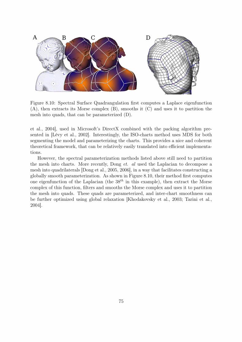
Figure 8.10: Spectral Surface Quadrangulation first computes a Laplace eigenfunction(A), then extracts its Morse complex (B), smooths it (C) and uses it to partition themesh into quads, that can be parameterized (D).

et al., 2004], used in Microsoft’s DirectX combined with the packing algorithm pre-sented in [Lévy et al., 2002]. Interestingly, the ISO-charts method uses MDS for bothsegmenting the model and parameterizing the charts. This provides a nice and coherenttheoretical framework, that can be relatively easily translated into efficient implementa-tions.

However, the spectral parameterization methods listed above still need to partitionthe mesh into charts. More recently, Dong et. al used the Laplacian to decompose amesh into quadrilaterals [Dong et al., 2005, 2006], in a way that facilitates constructing aglobally smooth parameterization. As shown in Figure 8.10, their method first computesone eigenfunction of the Laplacian (the 38th in this example), then extract the Morsecomplex of this function, filters and smooths the Morse complex and uses it to partitionthe mesh into quads. These quads are parameterized, and inter-chart smoothness canbe further optimized using global relaxation [Khodakovsky et al., 2003; Tarini et al.,2004].

75

Chapter 9

Cross-Parameterization / Inter-surface Map-ping

In a cross-parameterization or inter-surface-mapping setup the parameter domain forone mesh is another surface mesh. Cross-parameterization is used to morph or blendbetween meshes and to transfer properties between them. For morphing in addition toobtaining a mapping it is necessary to obtain a common compatible connectivity for thetwo meshes. The most common approach for pair-wise mapping is to parameterize bothmodels on a common base domain. Free-boundary planar parameterization is clearlyunsuitable for this purpose. Instead alternate domains such as a simplicial complex ora sphere are commonly used.

9.1 Base Complex Methods

Many methods use mapping to a common base-complex to obtain a cross-parameteriza-tion. Since the base must be shared the construction is significantly more challengingthan when parameterizing a single mesh. Praun et al. [2001] partition a mesh intotriangular patches, which correspond to the faces of a user given simplicial complex, bydrawing a network of paths between user-supplied feature vertices that correspond tothe vertices of the base mesh.

Schreiner et al. [2004] and Kraevoy and Sheffer [2004] extend the methods of Praunet al. [2001] and Kraevoy et al. [2003] to construct the simplicial complex automatically,in parallel to the patch formation. The input to both methods includes a set of corre-spondences between feature vertices on the two input models. The methods use those asthe vertices of the base complex. They simultaneously trace paths on the input meshesbetween corresponding pairs of vertices, splitting existing mesh edges if necessary.

Once the base is created, the meshes can be mapped to the base using the techniquesreviewed in the chapter on alternative domains. Schreiner et al. [2004] use an alternativeapproach. They never compute an explicit map between the full-resolution objectsand the base domain. Instead, they alternate the role of base domain between thetwo meshes, at various complexity levels in a multi-resolution representation. Theyprogressively refine each mesh by adding new vertices and relaxing their location using astretch-based metric measured on a temporary planar unfolding of their neighborhoods.

76

Figure 9.1: Base complex construction.

77

9.2 Energy driven methods

Several methods use an energy-driven approach for cross-parameterization, where onemesh is directly attracted towards the other [Allen et al., 2003; Sumner and Popović,2004]. The attraction energy function consists of components that pull the vertices ofone mesh towards nearest locations on the other while trying to preserve the shape of themesh as much as possible. To facilitate correspondence they require the user to specifyseveral dozen point-to-point correspondences between the input models. The methodswork well when the meshes are very similar, e.g. humans in the same pose [Allen et al.,2003] but tend to converge to a poor local minimum with increase in shape difference.These methods are quite sensitive to the weights used inside the energy functional toaccount for the different components. One advantage of these approaches is that theycan find mappings between models of different topology (genus, etc.), though these mapsare no longer bijective.

9.3 Compatible Remeshing

For applications such as morphing it is not enough to obtain a cross-parameterizationbetween the two models. For these applications, at the end of the process the two modelsare typically required to have the same connectivity. There are three main approachesfor generating such common connectivity.

• Base mesh subdivision: Several methods including [Praun et al., 2001] use thebase mesh connectivity and refine it using the one-to-four subdivision pattern,introducing as many levels of subdivision as necessary to capture the geometryof both models. The advantage of the method is simplicity. It’s drawback is thedependence on the shape of base mesh triangles. The method also tends to requirelarge triangle count to achieve acceptable accuracy (roughly factor 10 comparedto input mesh sizes).

• Overlay: Another approach for generating common connectivity [Alexa, 2000;Schreiner et al., 2004] is to intersect the two input meshes in the parameter domain,combining all their vertices and generating new vertices at edge-edge intersections.The method preserves exactly the input geometries but is not-trivial to implementand like subdivision increases the triangle count by roughly a factor of 10.

• Remeshing: In [Kraevoy and Sheffer, 2004] the authors propose an alternativewhere they use the connectivity of one of the input meshes as a basis and thenrefine it as necessary based on an approximation error with respect to the secondmesh. The resulting meshes have significantly lower triangle count than using theother two approaches. The result heavily depends on which of the inputs is selectedas the source for common connectivity. Unlike in the overlay approach, some finefeatures of the second mesh are only approximated and it is difficult to faithfullyreproduce sharp features.

78

Chapter 10

Numerical Optimization

In all the parameterization methods listed in the section above (Floater’s parameteriza-tion method, harmonic parameterization, conformal parameterization), we need eitherto solve a linear system or to minimize a quadratic objective function. A specificity ofthe numerical problems yielded in mesh parameterization is that the involved matricesare usually sparse. As a consequence, we will first explain how to efficiently implementa data structure for sparse matrices. To make user’s life easier, we propose an imple-mentation that can dynamically grow when coefficients are added to the matrix. AC++ version of this implementation is given in the companion material, based on thestd::vector data structure. This data structure is available in our Graphite software.We also provide a C version in OpenNL http://alice.loria.fr/software. Note thatthis data structure can be easily extended. Our C++ and C implementations also pro-vide the following features (not detailed in the implementation given in the appendix tokeep its length reasonable):

1. storage of the diagonal term

2. storage of both sparse rows and columns

3. symmetric storage (i.e., do not store the upper triangle for symmetric matrices)

4. non-square matrices

5. matrix × matrix multiply

Features (1) and (2) are interesting for implementing Jacobi preconditioner (re-quires 1) or SSOR preconditioner (requires 1+2). Feature (3) speeds up the conjugategradient algorithm (but requires some modification in the matrix × vector routine).Features (4) and (5) can be used by more sophisticated non-linear solvers (such as MIPSand ABF).

Numerical methods are a particularly efficient formalism for geometric modelingproblems that involve large meshes. The approach consists in formalizing the problemas a function of many variables and optimizing it. The variables correspond to values(e.g., coordinates, colors, texture coordinates, etc.) attached to the vertices of the mesh.

79

1

2 3 4

5 6

7 8 9

0

1

2

3

0 1 2 3j

i 1 2 3 4 5 6 7 8 9

0 1 2 3 4 5 6 7 8

0 1 1 1 2 2 3 3 3

a

i

9=NNZ

1 0 2 3 1 3 1 2 3j

Figure 10.1: Example of sparse matrix with TRIAD format

These numerical optimization problems involve large matrices, defined from the meshand the values attached to the vertices and/or the edges and/or the facets of the mesh. Inmost cases, these matrices are sparse (and have a structure identical or strongly relatedwith the adjacency matrix of the graph formed by the mesh). We start this section byreviewing some efficient data structures to represent sparse matrices.

10.1 Data structures for sparse matrices

Algorithm 1 TRIAD data structure for sparse matricesstruct TRIADMatrix

int N ; // dimension of the matrixint NNZ ; // number of non-zero coefficientsdouble* a ; // non-zero coefficients (array of size NNZ)int* I ; // row indices (array of size NNZ)int* J ; // column indices (array of size NNZ)

;

Algorithm 2 Matrix × vector product with the TRIAD data structurevoid mult(double* y, TRIADMatrix* M, double* x)

for(int i=0; i<M->N; i++) y[i] = 0.0 ;

for(int k=0; k<M->NNZ; k++)

y[M->I[k]] += M->a[k] * x[M->J[k]] ;

80

1

2 3 4

5 6

7 8 9

0

1

2

3

0 1 2 3j

i 1 2 3 4 5 6 7 8 9

0 1 2 3 4 5 6 7 8

1 0 2 3 1 3 1 2 3

0 1 4 6 9

a

colind

rowptr

9=NNZ

Figure 10.2: Example of sparse matrix represented in the CRS format.

10.1.1 TRIAD data structure

To optimize the storage of sparse matrices, the first idea that comes naturally to mindconsists in storing only the non-zero coefficients, with the associated (i, j) indices. There-fore, instead of storing n2 coefficients, we only need to store NNZ coefficients (NNZ:Number of Non-Zero coefficients) and the same number of (i, j) indices. This datastructure is referred to as the TRIAD format, depicted in Figure 10.1. We also show animplementation in C (Algorithm 1). The function that computes the product between asparse matrix in TRIAD format and a vector is given by Algorithm 2). For instance, thisfunction is particularly useful to implement a solver based on the Conjugate Gradientmethod (see below).

Despite the obvious gain realized by the TRIAD format as compared to a regular2D array, this representation still shows a high redundancy of the coefficients i, thatstore the row index associated to each entry. For this reason, this format is seldom usedin numerical libraries (it is limited to input file formats, since its simplicity favors itsunderstanding and use). In practice, the CRS (Compressed Row Storage) data structureis preferred, since it is more compact in memory. We detail this format in the nextsubsection.

Algorithm 3 Compressed Row Storage data structure for sparse matricesstruct CRSMatrix

int N ; // dimension of the matrixint NNZ ; // number of non-zero coefficientsdouble* a ; // non-zero coefficients (array of size NNZ)int* colind ; // column indices (array of size N)int* rowptr ; // row pointers (array of size N+1)double* diag ; // diagonal elements (array of size N)

;

81

10.1.2 Compressed Row Storage

The CRS format (Compressed Row Storage) is one of the most commonly used datastructure for sparse matrices, used in large numerical libraries. The transposed vari-ant CCS (Compressed Column Storage) is also used (depending on the algorithms andimplementation choices). We present here the CRS format. Algorithm 3 presents theimplementation in C, and Figure 10.2 shows an example. The CRS data structure usesthree indices to represent non-zero coefficients and their indices. As in the TRIAD for-mat, the array a stores all the non-zero entries. The array colind gives for each entrythe corresponding column index. The rows are encoded in a different, more compactmanner, by the rowptr array. This array gives for each row its start and end in thearrays a and colind. To facilitate the coding of algorithm, a common practice consistsin completing the array colind by an additional entry, that points one entry past thelast entry of the matrix. This additional entry of colind is called a sentry and avoids atest in the matrix × vector product, as shown below.

Algorithm 4 Matrix × vector product with the CRS formatvoid mult(double* y, CRSMatrix* M, double* x)

for(int i=0; i<M->N; i++) y[i] = 0.0 ;for(int jj=M->rowptr[i]; jj<M->rowptr[i+1]; jj++)

y[i] += M->a[jj] * x[M->colind[jj]] ;

Algorithm 4 shows how to implement the product between a sparse matrix M storedin the CRS format and a vector x. The sentry rowptr[N] = NNZ avoids to have aparticular case for the last row of the matrix.

Different versions of the CRS data structure exist. Thus, if the matrix is symmetric,it is possible to save some memory by only storing the lower triangular part of the matrix.Other variants store the diagonal coefficients in a separate array, to facilitate the imple-mentation of the Jacobi preconditioner (see below). Other variants store the columnsinstead of the rows (CCS: Compressed Column Storage). Finally, the BCRS (BlockCompressed Row Storage) partitions the matrix into fixed size blocks and stores themin the CRS format. This both optimizes memory accesses, and favors using extendinginstruction sets (e.g. SSE on Intel Processor).

The CRS data structure and its variants are both compact and efficient. However,in our particular context of numerical problems related with geometric optimization of3D meshes, the CRS data structure is somewhat too rigid, as explained below. In ageometric optimization problem, it is natural to assemble the matrix by traversing thegraph that corresponds to the mesh. During the traversal, coefficients are accumulatedin the matrix, generated by elementary neighborhoods (called stencils in finite elementsparlance). Since the CRS data structure requires to define the number of non-zero

82

1

2 3 4

5 6

7 8 9

0

1

2

3

0 1 2 3j

i

(a ,j)i,j

(1,1)

(2,0) (3,2) (4,3)

(5,1) (6,3)

(7,1) (8,2) (9,3)

row[0]

row[1]

row[2]

row[3]

Figure 10.3: Dynamic sparse matrix data structure

coefficients in advance, constructing a CRS matrix requires two traversals of the graph.The first traversal determines the non-zero pattern, i.e. the set of (i, j) index couplessuch that ai,j is non-zero. Then, the data structure is allocated in memory. Finally, asecond traversal computes the numerical values of the ai,j entries. In practice, this wayof proceeding is uncomfortable to implement. For this reason, we propose a dynamicmatrix data structure, for which the number of non-zero coefficients can vary. Theimplementation is available in our library OpenNL and in the Graphite platform (http://alice.loria.fr/software).

10.1.3 Dynamic matrices

Our dynamic sparse matrix is built around the class std::vector of the standard C++library (STL for Standard Template Library). This container class show the interestingcapability of growing in memory while minimizing the number of required copies1. Thus,our dynamic sparse matrix data structure, depicted in Figure 10.3, and detailed inAlgorithm 5, consists of an array row. Each row is implemented by a std::vector ofvalue-index pairs, and each pair is represented by an instance of the Coeff structure.The whole data structure shows a memory storage requirement comparable to the CRSformat, while offering better flexibility. This flexibility is exposed to the user by thefunction add(i,j,val), that adds the value val to the coefficient ai,j.

The matrix-vector product remains simple to implement with this structure. Thesource code is given in Algorithm 6. However, it is important to notice that this betterflexibility is obtained at the expense of lower performances of the matrix × vectorproduct (approximately by a factor of 2 in our experimentation). This can be explainedby the loss of data locality, that results in less efficient cache usage as compared tothe CRS representation. For this reason, in the case where a large number of matrix

1This is done by doubling the size of the memory space allocated to the container each time a copyoperation is necessary. This makes the number of copies decrease as a function of the log of the finalsize.

83

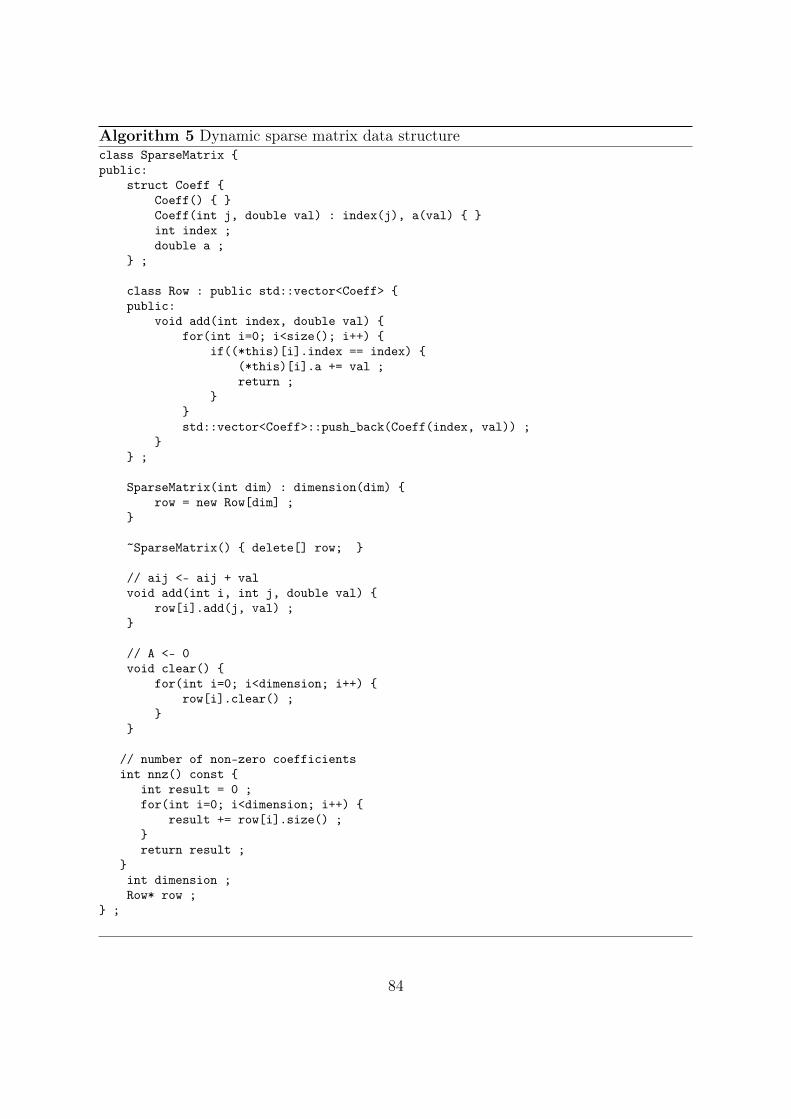
Algorithm 5 Dynamic sparse matrix data structureclass SparseMatrix public:

struct Coeff Coeff() Coeff(int j, double val) : index(j), a(val) int index ;double a ;

;

class Row : public std::vector<Coeff> public:

void add(int index, double val) for(int i=0; i<size(); i++)

if((*this)[i].index == index) (*this)[i].a += val ;return ;

std::vector<Coeff>::push_back(Coeff(index, val)) ;

;

SparseMatrix(int dim) : dimension(dim) row = new Row[dim] ;

~SparseMatrix() delete[] row;

// aij <- aij + valvoid add(int i, int j, double val)

row[i].add(j, val) ;

// A <- 0void clear()

for(int i=0; i<dimension; i++) row[i].clear() ;

// number of non-zero coefficientsint nnz() const

int result = 0 ;for(int i=0; i<dimension; i++)

result += row[i].size() ;return result ;

int dimension ;Row* row ;

;

84

Algorithm 6 Matrix × vector product with the dynamic data structure// y <- Mxvoid mul(double* y, const SparseMatrix& M, const double* x)

for(int i=0; i<M.dimension; i++) y[i] = 0 ;const Row& R = M.row[i] ;for(int jj=0; jj<R.size(); jj++)

y[i] += R[jj].a * x[ R[jj].index ] ;

Algorithm 7 Converting a dynamic sparse matrix into the CRS formatvoid convert_to_CRS(

const SparseMatrix& M,CRSMatrix& M_CRS,int array_base // 0 for C, 1 for Fortran

) M_CRS.N = M.dimension ;M_CRS.NNZ = M.nnz() ;M_CRS.A = new double[M_CRS.NNZ] ;M_CRS.col_ind = new int[M_CRS.NNZ] ;M_CRS.row_ptr = new int[M_CRS.N+1] ;int count = 0 ;for(int i=0; i<M_CRS.N; i++)

const SparseMatrix::Row& R = M.row[i] ;M_CRS.row_ptr[i] = count + array_base ;for(int jj=0; jj<R.size(); jj++)

M_CRS.a[count] = R[jj].a ;M_CRS.col_ind[count] = R[jj].index + array_base ;count++ ;

M_CRS.col_ptr[M_CRS.N] = M_CRS.NNZ + array_base ;

85

× vector products need to be computed (e.g., in a Conjugate-Gradient based iterativesolver described later), it may be more efficient to convert the dynamic matrix into theCRS format. The conversion routine can be also used to interface the dynamic matrixdata structure with sparse direct solvers (SuperLU, TAUCS, MUMPS, etc.) that usethe CRS format. The source code of the conversion routine is given in Algorithm 7.This function is not difficult to implement. The only thing that one needs to take careof is the additional parameter array_base that deserves some explanations. The C andFORTRAN languages do not use the same convention for array indexing. The first entryof an array is indexed by 0 in C, and by 1 in FORTRAN. For this reason, if the CRSmatrix is meant to be used by a FORTRAN routine, this parameter needs to be set to 1.

Now that we have seen the elementary data structures for sparse matrices, the algo-rithm to manipulate them and their implementation in C and C++, we will see somepopular algorithms to solve linear systems.

10.2 Solving Linear Systems

A wide class of geometric modeling problems require to solve a large sparse linear system,i.e. an equation of the form Ax = b, with A that denotes a n × n non-singular squarematrix, b a vector of dimension n, and x the unknown vector (of dimension n). In thissection, we describe several methods to solve these linear systems.

10.2.1 Relaxation

The relaxation method is the most simple, both from the conceptual and the implemen-tation points of view. This method was widely used in the 90’s to implement geometryprocessing algorithm. It was then later replaced by more efficient algorithms, listedbelow.

The relaxation method can be easily understood by considering the problem Ax = bas a linear system: ⎧⎪⎪⎪⎪⎪⎨

⎪⎪⎪⎪⎪⎩

a1,1x1 +a1,2x2 + . . . +a1,nxn = b1...

ai,1x1 +ai,2x2 + . . . +ai,nxn = bi...

an,1x1 +an,2x2 + . . . +an,nxn = bn

The method consists in traversing the equations one by one, and compute for eachequation i the value of xi obtained by pretending that all the other variables xj for j = iare known. This gives the following update scheme for the variable xi:

xi ←1

ai,i

(bi −

∑j =i

ai,jxj

)

86

The complete algorithm for the relaxation method then writes:

while ‖Ax− b‖ < εfor i from 1 to n

xi ← 1ai,i

(bi −

∑j =i ai,jxj

)end//for

end//while

with ε the precision specified by the user. It is also possible to specify a maximumnumber of iterations, so that the algorithm stops even if it does not converge.

As can be seen, this algorithm cannot be applied to matrices with zero values on thediagonal. More generally, it is possible to prove a sufficient condition for convergence.If the matrix is diagonal dominant, i.e.

∀i,∀j = i, |ai,i| > |ai,j|then the algorithm converges.

It is possible to speed-up this algorithm, by using the fact that the update appliedto each variable xi “points toward the right direction”. Intuitively, going “a bit further”in that direction, by multiplying the displacement by a factor ω, is likely to acceleratethe speed of convergence. The so-modified update scheme writes:

xprev ← xi

xi ← 1ai,i

(bi −

∑j =i ai,jxj

)xi ← xprev + ω(xi − xprev)

This update scheme first computes the update of xi as before, and then multiplies thisdisplacement relative to the previous value xprev by a factor ω. It is possible to provethat the algorithm converges under the same conditions as relaxation (diagonal dominantmatrix), and for ω ∈ [1, 2[. The so-modified algorithm is referred to as SOR (successiveover-relaxation). By rewriting the update scheme in a more compact form, the completeSOR algorithm is given by:

while ‖Ax− b‖ < εfor i from 1 to n

xi ← (1− ω)xi + ωai,i

(bi −

∑j =i ai,jxj

)end//for

end//while

The optimal choice for the parameter ω is determined by the eigenvalues of the matrixA. Generally, computing those eigenvalues is much more expensive than solving thesystem. For this reason, either a theoretical study of the numerical problem can givethe optimal ω, or it is determined in an empirical way.

The main advantage of the SOR method is its simplicity, from both the conceptualand implementation point of view. This simplicity favored its use in the geometryprocessing community [Taubin, 1995]. However, as we will see later, the community nowuses more efficient methods, such as the conjugate gradient and sparse direct solvers.

87

10.2.2 The conjugate gradient method

The conjugate gradient method is much more efficient, and does not require much effortsto be implemented. This algorithm is based on the equivalence between solving the linearsystem Ax = b and minimizing the quadratic form F (x) = 1/2xtAx−btx. More precisely,the algorithm computes a basis of vectors that is orthogonal in the space of the matrix(i.e. a basis of conjugate vectors), by applying the Gram-Schmidt orthogonalizationalgorithm. Fortunate simplifications in the computations make it possible to obtain thevectors of the basis one by one, by only keeping one vector in memory. The next one isthen obtained as a linear combination of the previous one and the gradient ∇F = Ax−bat the current point x. The complete algorithm writes:

Algorithm 8 Pre-conditioned Conjugate Gradienti← 0; r← b−Ax; d←M−1r;δnew ← rTd; δ0 ← δnew;while i < imax et δnew > ε2δ0

q← Ad; α← δnew

dT q;

x← x + αd; r← r− αq;s←M−1r; δold ← δnew;δnew ← rT s; β ← δnew

δold;

d← r + βd; i← i + 1;end

In this algorithm, the matrix M , called a preconditioner, allows to speed-up thespeed of convergence of the algorithm. For instance, the Jacobi preconditioner is simplyequal to the diagonal terms of the matrix A. More sophisticated preconditioners exist,however, our experiments have shown that reasonably efficient results are obtained withthe Jacobi preconditioner.

As can be seen in this algorithm, the most complicated operation is a matrix ×vector product. All the other computations are simply dot products between vectors,and linear combinations of vectors.

The conjugate gradient method cannot be applied to non-symmetric matrices. Fora non-symmetric matrix, it is possible to apply the conjugate gradient method to thenormal equation AtAx = Atb. The resulting method is called conjugate gradient squared(CGSQ). However, since this squares the condition number, the loss of numerical stabilitymakes this method not suitable in general.

Another idea consists in deriving from the system Ax = b an equivalent symmetricsystem, as follows: (

Id AAt 0

)(0x

)=

(b0

)It is then possible to applied the conjugate gradient method to this system. This definesthe BiCG algorithm Bi Conjugate Gradient. A variant named BiCGSTAB (stabilizedBiCG) accelerates the speed of convergence.

88

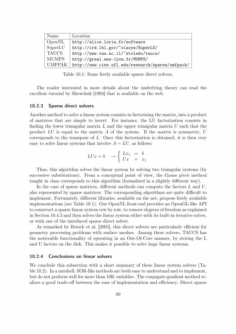
Name LocationOpenNL http://alice.loria.fr/softwareSuperLU http://crd.lbl.gov/~xiaoye/SuperLU/TAUCS http://www.tau.ac.il/~stoledo/taucs/MUMPS http://graal.ens-lyon.fr/MUMPS/UMFPAK http://www.cise.ufl.edu/research/sparse/umfpack/

Table 10.1: Some freely available sparse direct solvers.

The reader interested in more details about the underlying theory can read theexcellent tutorial by Shewchuk [1994] that is available on the web.

10.2.3 Sparse direct solvers

Another method to solve a linear system consists in factorizing the matrix, into a productof matrices that are simple to invert. For instance, the LU factorization consists infinding the lower triangular matrix L and the upper triangular matrix U such that theproduct LU is equal to the matrix A of the system. If the matrix is symmetric, Ucorresponds to the transpose of L. Once this factorization is obtained, it is then veryeasy to solve linear systems that involve A = LU , as follows:

LUx = b →

Lx1 = bUx = x1

Thus, this algorithm solves the linear system by solving two triangular systems (bysuccessive substitutions). From a conceptual point of view, the Gauss pivot methodtaught in class corresponds to this algorithm (formalized in a slightly different way).

In the case of sparse matrices, different methods can compute the factors L and U ,also represented by sparse matrices. The corresponding algorithms are quite difficult toimplement. Fortunately, different libraries, available on the net, propose freely availableimplementations (see Table 10.1). Our OpenNL front-end provides an OpenGL-like APIto construct a sparse linear system row by row, to remove degrees of freedom as explainedin Section 10.4.3 and then solves the linear system either with its built-in iterative solver,or with one of the interfaced sparse direct solver.

As remarked by Botsch et al. [2005], this direct solvers are particularly efficient forgeometry processing problems with surface meshes. Among these solvers, TAUCS hasthe noticeable functionality of operating in an Out-Of-Core manner, by storing the Land U factors on the disk. This makes it possible to solve huge linear systems.

10.2.4 Conclusions on linear solvers

We conclude this subsection with a short summary of these linear system solvers (Ta-ble 10.2). In a nutshell, SOR-like methods are both easy to understand and to implement,but do not perform well for more than 10K variables. The conjugate-gradient method re-alizes a good trade-off between the ease of implementation and efficiency. Direct sparse

89

method pros consrelaxation - SOR easy to implement inefficient

low memory costconjugate gradient easy to implement reasonably efficient

low memory costdirect methods the most efficient high memory cost

public codes available implementations are complex

Table 10.2: Classes of linear solver, pros and cons.

solvers are the most efficient, but may sometimes consumes considerable amounts ofRAM. Finally, direct solvers with Out-Of-Core storage [Meshar et al., 2006] let the userbenefit from the high efficiency of sparse direct solvers while keeping the control of theused amount of RAM.

10.3 Functions of many variables

We now focus on functions F : x → F (x) from Rn to R. For instance, such a function

can formalize the geometric criterion that should be met by a surface. In this context,the arguments of the functions is a vector x that gathers all the coordinates at all thevertices of the mesh. The function returns a real number that measures the “fairness” ofthe so-described geometry (in the usual definitions, lower values of this quantity corre-spond to a better quality). The optimization algorithm then seeks for the parameters ofthe function—i.e. the coordinates at the vertices—that minimize the function. In thiscontext, such a function is also called an “energy”, or an “objective function”. Variationalmethods minimize an objective function by studying the variations of F (x) in functionof the parameters x = [x1, . . . xn]. These variations are formalized by the derivatives ofF (x). More specifically, we will focus on methods that operate at order 2. This requiresto define the notion that corresponds to the first order derivative for multivariate func-tions (called the gradient) and the one that corresponds to the second order derivative(called the Hessian). We will then study some theorems that facilitate the computationsin expressions that combine the derivatives of F .

10.3.1 The gradient

The differential information at order 1 is represented by the vector of all derivativesrelative to all variables, called the gradient of F , and denoted by ∇F :

∇F =

⎡⎢⎢⎢⎢⎢⎣

∂F/∂x1...

∂F/∂xi...

∂F/∂xn

⎤⎥⎥⎥⎥⎥⎦

90

P1

P2

P3

P4

P5

Figure 10.4: Stationary points. The points P1 and P4 are local maxima, P2 is aninflexion point, P5 is a local minimum and P3 is the global minimum.

The notion of gradient is very useful in minimization, since a minimum is character-ized by the fact that the gradient of F is zero (if F is C1). However, the zero-set of thegradient (also called the set of stationary points) also contains other points, as shown inFigure 10.4 for the univariate case. First, a minimum can be local (rather than global),but the situation can be even worse: a stationary point can also be a (local or global)maximum. It can also be an inflexion point. To further characterize a stationary point,it is also necessary to check the sign of the second order derivative.

We now give little theorems that facilitate calculation with gradients:

(1) ‖x‖2 = xtx

(2) ∇(btx) = ∇(xtb) = b

(3) ∇(xtAx) = (A + At)x = 2Ax if A is symmetric

(1) is just an easy way of unifying the squared norm of a vector and matrix products(we will use it later). (2) is also trivial. To prove (3), we expand xtAx and compute itsderivatives relative to the variables xi:

91

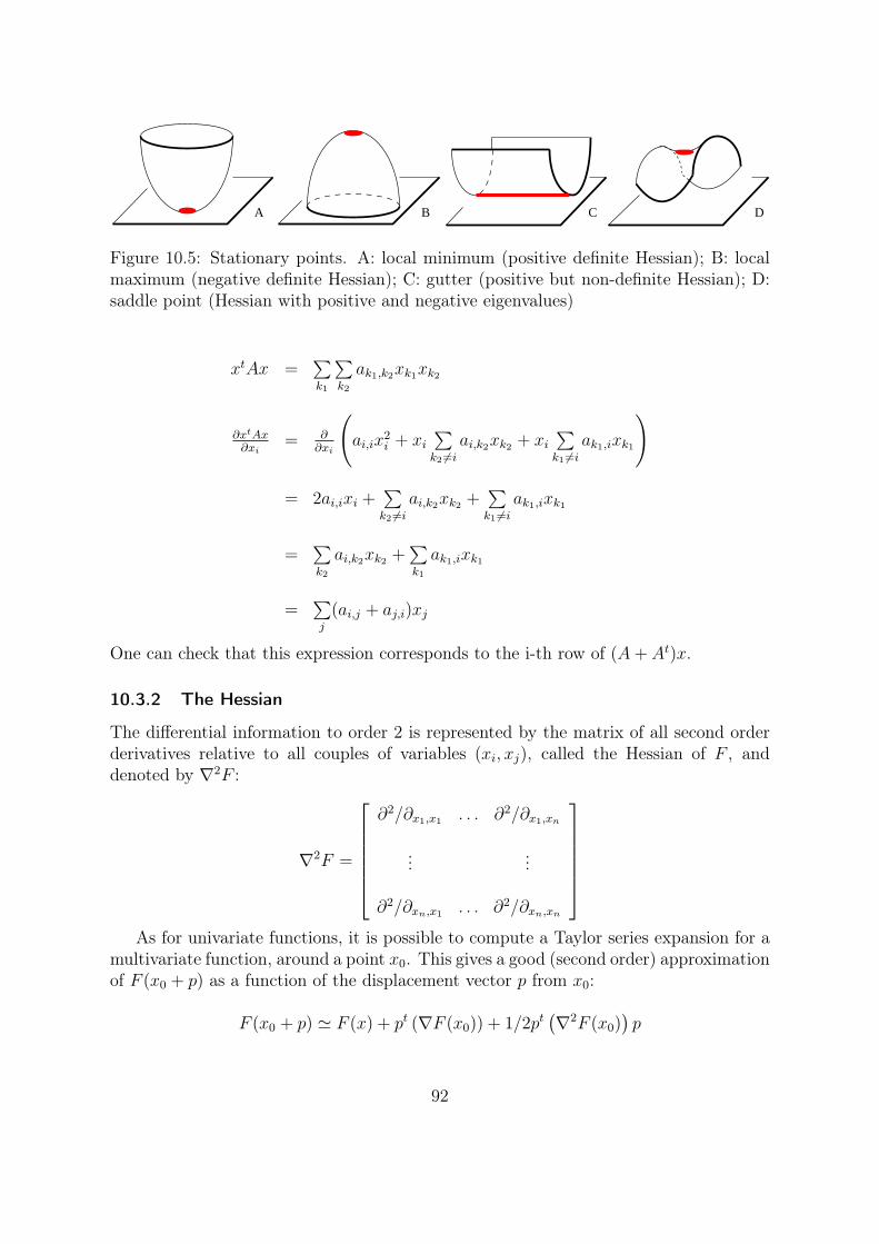
A B C D

Figure 10.5: Stationary points. A: local minimum (positive definite Hessian); B: localmaximum (negative definite Hessian); C: gutter (positive but non-definite Hessian); D:saddle point (Hessian with positive and negative eigenvalues)

xtAx =∑k1

∑k2

ak1,k2xk1xk2

∂xtAx∂xi

= ∂∂xi

(ai,ix

2i + xi

∑k2 =i

ai,k2xk2 + xi

∑k1 =i

ak1,ixk1

)

= 2ai,ixi +∑

k2 =i

ai,k2xk2 +∑

k1 =i

ak1,ixk1

=∑k2

ai,k2xk2 +∑k1

ak1,ixk1

=∑j

(ai,j + aj,i)xj

One can check that this expression corresponds to the i-th row of (A + At)x.

10.3.2 The Hessian

The differential information to order 2 is represented by the matrix of all second orderderivatives relative to all couples of variables (xi, xj), called the Hessian of F , anddenoted by ∇2F :

∇2F =

⎡⎢⎢⎢⎢⎢⎣

∂2/∂x1,x1 . . . ∂2/∂x1,xn

......

∂2/∂xn,x1 . . . ∂2/∂xn,xn

⎤⎥⎥⎥⎥⎥⎦

As for univariate functions, it is possible to compute a Taylor series expansion for amultivariate function, around a point x0. This gives a good (second order) approximationof F (x0 + p) as a function of the displacement vector p from x0:

F (x0 + p) F (x) + pt (∇F (x0)) + 1/2pt(∇2F (x0)

)p

92

As previously mentioned, the Hessian gives more information about a stationarypoint. Figure 10.5 shows some configurations that can be encountered in the case of afunction of two variables. According to the sign of the eigenvalues of the Hessian, theconfiguration is a local minimum (A), a local maximum (B), a gutter (C), or a saddlepoint (D). Therefore, to minimize a function F , finding the zero-set of the gradient is ingeneral not sufficient. One also needs to check the sign of the eigenvalues of the Hessian.Even if they are positive, this may be a local minimum.

10.4 Quadratic Optimization

10.4.1 Quadratic Forms

A quadratic form is a polynomial function such that the degree of its terms is not largerthan 2. It is always possible to write a quadratic form as follows:

F (x) = 1/2xtGx + xtc + α

where G is a n × n symmetric matrix, c is a vector of Rn, and α a scalar. Finding the

stationary point(s) of a quadratic form is quite easy, by studying its gradient:

∇F (x) = 0⇔ Gx + c = 0

Thus, minimizing a quadratic form or solving a symmetric linear system are two problemsthat are equivalent.

10.4.2 Least squares

We suppose that we want to solve a linear system of equations such that the number mof equations is greater than the number n of variables:⎧⎪⎨

⎪⎩a1,1x1 + . . . + a1,nxn = b1

...am,1x1 + . . . + am,nxn = bm

or Ax = b. In the general case, the system has no solution. It is then possible to tryto find the “least bad” solution, i.e. the vector x that minimizes the sum of the squaredresiduals:

F (x) =m∑

i=1

(n∑

j=1

ai,jxj − bi

)2

= ‖Ax− b‖2

The function F is a quadratic form, that can be written as follows (Theorem (1)):

F (x) = ‖Ax− b‖2 = (Ax− b)t(Ax− b) = xtAtAx− 2xtAtb + btb

(the two terms xtAtb and btAx are equal, since they are scalars, or 1 × 1 matrices,that are symmetric). The vector x that minimizes F is such that ∇F = 0. Therefore(Theorems (2) and (3)):

∇F (x) = 2AtAx− 2Atb = 0

93

We retrieve the classical formula for the least squares, also called linear regression. Thevector x that minimizes ‖Ax− b‖2 satisfies AtAx = Atb.

10.4.3 Least squares with reduced degrees of freedom

For some algorithms, it may be useful to remove some degrees of freedom of the system,by fixing some parameters of the objective function. Formally, this means that the vectorx of parameters is partitioned into two sub-vectors x = [xf |xl]. The first nf componentsxf = [x1 . . . xf ] correspond to the free parameters, and the remaining n−nf componentsxl = [xnf+1 . . . xn] correspond to the locked parameters. Thus, the function F solelydepends on the vector xf , and rewrites:

F (xf ) = ‖Ax− b‖2 =

∥∥∥∥∥∥∥∥[Af | Al]

⎡⎢⎢⎣

xf

xl

⎤⎥⎥⎦− b

∥∥∥∥∥∥∥∥2

Partitioning the vector x into two subvectors [xf , xl] naturally partitions the matrixA into two submatrices Af , Al (in the product Ax, the coefficients of A that weightparameters in xf are in Af , and those that weight parameters in xl are in Al). It is thenpossible to isolate the terms that depend of xf :

F (xf ) = ‖Afxf + Alxl − b‖2

By introducing b′ = Alxl − b, and by using the least-squares formula proved in theprevious section, one retrieves the equation satisfied by the minimizer xf of F :

AtfAfxf = At

fb′ or At

fAfxf = Atfb− At

fAlxl

10.5 Non-linear optimization

We now focus on the more difficult problem of minimizing non-linear functions. In thissection, we present the Newton method, that can compute a stationary point of a non-linear function. Other methods exist and the interested reader may read reference books[Nocedal and Wright, 2006] for more details.

10.5.1 Univariate functions

We first consider the case of a univariate function. The following algorithm iterativelycomputes a stationary point of the function f :

while |f ′(x)| > εp← −f ′(x)/f ′′(x)x← x + p

end // while

94

The algorithm works as follows: at each step, we compute the second order of thefunction f around the current point x. This approximation is called a model function,since it gives a good approximation (or a good model) of the variations of f around xin function of a displacement p:

f(x + p) fx(p) = f(x) + pf ′(x) + p2/2f ′′(x)

Then, the algorithm computes the displacement p that minimizes the model function.This gives:

f ′x(p) = 0

f ′(x) + pf ′′(x) = 0p = −f ′(x)/f ′′(x)

Finally, the current location is updated: x ← x + p, and the algorithm iterates all theprevious steps.

10.5.2 Multivariate functions

The previous (univariate) algorithm can be easily adapted to the multivariate case. Aswe have seen in the previous section, the second order Taylor expansion of a multivariatefunction F writes:

F (x + p) Fx(p) = F (x) + pt (∇F (x)) + 1/2pt(∇2F (x)

)p

It is clearly a quadratic form. We then find the displacement p p that minimizes thisquadratic form:

∇Fx(p) = 0(∇F (x)) + (∇2F (x)) p = 0

p = − (∇2F (x))−1

(∇F (x))

The Newton algorithm for multivariate functions can then be given by:

while ‖∇F (x)‖ > εsolve (∇2F (x))p = −(∇F (x))x← x + p

end // while

In other words, to minimize a non-linear function, the Newton algorithm minimizesa series of quadratic form (by solving a series of linear systems). To solve those linearsystems, one may use one of the methods listed in Section 10.2.

95

10.6 Constrained Optimization: Lagrange Method

We now focus on the problem of constrained optimization. A constrained optimizationproblem can be formalized by:

minimizeF (x) with

⎧⎪⎪⎪⎨⎪⎪⎪⎩

G1(x) = 0G2(x) = 0

...Gm(x) = 0

where F and G1, G2 . . . Gm are functions from Rn to R. The functions Gi are called

constraints. An important theorem, known as the KKT condition2, states that theminimizer of F that satisfies the Gi constraints is also a stationary point of the functionL, defined by:

L(x, λ) = F (x) +m∑

i=1

λiGi(x)

The function L, called the Lagrangian of the constrained optimization problem, dependsof m additional λi parameters, associated with the m constraints Gi.

The stationary points of the Lagrangian L can be found by the Newton method,presented in the previous section.

2Named after its authors, Karush, Kuhn and Tucker

96

Bibliography

J. H. Ahlberg, E. N. Nilson, and J. L. Walsh. The theory of splines and their applications.Academic Press, New York, 1967.

B. Aksoylu, A. Khodakovsky, and P. Schröder. Multilevel solvers for unstructured surfacemeshes. SIAM Journal on Scientific Computing, 26(4):1146–1165, 2005.

M. Alexa. Merging polyhedral shapes with scattered features. The Visual Computer, 16(1):26–37, 2000.

M. Alexa. Recent advances in mesh morphing. Computer Graphics Forum, 21(2):173–196, 2002.

B. Allen, B. Curless, and Z. Popović. The space of human body shapes: reconstructionand parameterization from range scans. ACM Transactions on Graphics, 22(3):587–594, 2003. Proceedings of SIGGRAPH 2003.

P. Alliez and C. Gotsman. Recent advances in compression of 3D meshes. In N. A.Dodgson, M. S. Floater, and M. A. Sabin, editors, Advances in Multiresolution forGeometric Modelling, Mathematics and Visualization, pages 3–26. Springer, Berlin,Heidelberg, 2005.

P. Alliez, D. Cohen-Steiner, O. Devillers, B. Lévy, and M. Desbrun. Anisotropic polyg-onal remeshing. ACM Transactions on Graphics, 22(3):485–493, 2003. Proceedings ofSIGGRAPH 2003.

P. Alliez, G. Ucelli, C. Gotsman, and M. Attene. Recent advances in remeshing ofsurfaces. Research report, AIM@SHAPE Network of Excellence, 2005.

D. Anguelov, P. Srinivasan, D. Koller, S. Thrun, J. Rodgers, and J. Davis. SCAPE:Shape completion and animation of people. ACM Transactions on Graphics, 24(3):408–416, 2005. Proceedings of SIGGRAPH 2005.

N. Arad and G. Elber. Isometric texture mapping for free-form surfaces. ComputerGraphics Forum, 16(5):247–256, 1997.

P. N. Azariadis and N. A. Aspragathos. On using planar developments to perform texturemapping on arbitrarily curved surfaces. Computers & Graphics, 24(4):539–554, 2000.

97

L. Balmelli, G. Taubin, and F. Bernardini. Space-optimized texture maps. ComputerGraphics Forum, 21(3):411–420, 2002. Proceedings of Eurographics 2002.

A. Belyaev. On transfinite barycentric coordinates. In Proceedings of the 4th Euro-graphics Symposium on Geometry Processing (SGP 2006), pages 89–99. EurographicsAssociation, 2006.

C. Bennis, J.-M. Vézien, and G. Iglésias. Piecewise surface flattening for non-distortedtexture mapping. ACM SIGGRAPH Computer Graphics, 25(4):237–246, 1991. Pro-ceedings of SIGGRAPH ’91.

E. Bier and K. Sloan. Two-part texture mappings. IEEE Computer Graphics andApplications, 6(9):40–53, 1986.

H. Biermann, I. Martin, F. Bernardini, and D. Zorin. Cut-and-paste editing of multires-olution surfaces. ACM Transactions on Graphics, 21(3):312–321, 2002. Proceedingsof SIGGRAPH 2002.

H. Birkholz. Shape-preserving parametrization of genus 0 surfaces. In Proceedings of the12th International Conference in Central Europe on Computer Graphics, Visualizationand Computer Vision (WSCG 2004), pages 57–64, 2004.

V. Blanz and T. Vetter. A morphable model for the synthesis of 3D faces. In Proceedingsof SIGGRAPH ’99, pages 187–194. ACM Press, 1999.

V. Blanz, C. Basso, T. Poggio, and T. Vetter. Reanimating faces in images and video.Computer Graphics Forum, 22(3):641–650, 2003. Proceedings of Eurographics 2003.

V. Blanz, K. Scherbaum, T. Vetter, and H.-P. Seidel. Exchanging faces in images.Computer Graphics Forum, 23(3):669–676, 2004. Proceedings of Eurographics 2004.

J. F. Blinn. Simulation of wrinkled surfaces. ACM SIGGRAPH Computer Graphics, 12(3):286–292, 1978. Proceedings of SIGGRAPH ’78.

I. Boier-Martin, H. Rushmeier, and J. Jin. Parameterization of triangle meshes overquadrilateral domains. In Proceedings of the Second Eurographics Symposium onGeometry Processing (SGP 2004), pages 193–203. Eurographics Association, 2004.

M. Botsch, D. Bommes, and L. Kobbelt. Efficient linear system solvers for mesh process-ing. In Mathematics of Surfaces XI, volume 3604 of Lecture Notes in Computer Sci-ence, pages 62–83. Springer, Berlin, Heidelberg, 2005. Proceedings of the 11th IMAInternational Conference.

P. L. Bowers and M. K. Hurdal. Planar conformal mappings of piecewise flat surfaces. InH.-C. Hege and K. Polthier, editors, Visualization and Mathematics III, pages 3–34.Springer, Heidelberg, 2003.

98

S. C. Brenner and L. R. Scott. The mathematical theory of finite element methods,volume 15 of Texts in Applied Mathematics. Springer, second edition, 2002.

S. Campagna and H.-P. Seidel. Parameterizing meshes with arbitrary topology. InProceedings of Image and Multidimensional Digital Signal Processing ’98, pages 287–290, 1998.

N. A. Carr and J. C. Hart. Meshed atlases for real-time procedural solid texturing. ACMTransactions on Graphics, 21(2):106–131, 2002.

N. A. Carr and J. C. Hart. Painting detail. ACM Transactions on Graphics, 23(3):587–594, 2004. Proceedings of SIGGRAPH 2004.

N. A. Carr, J. Hoberock, K. Crane, and J. C. Hart. Rectangular multi-chart geometryimages. In Proceedings of the 4th Eurographics Symposium on Geometry Processing(SGP 2006), pages 181–190. Eurographics Association, 2006.

G. Choquet. Sur un type de transformation analytique généralisant la représentationconforme et définé au moyen de fonctions harmoniques. Bulletin des Sciences Mathé-matiques, 69:156–165, 1945.

F. R. K. Chung. Spectral Graph Theory. Number 92 in CBMS Regional ConferenceSeries in Mathematics. American Mathematical Society, 1997.

B. Cipra. You can’t always hear the shape of a drum. In What’s Happening in theMathematical Sciences, volume 1. American Mathematical Society, Providence, RI,1993.

U. Clarenz, N. Litke, and M. Rumpf. Axioms and variational problems in surface para-meterization. Computer Aided Geometric Design, 21(8):727–749, 2004.

D. Cohen-Steiner, P. Alliez, and M. Desbrun. Variational shape approximation. ACMTransactions on Graphics, 23(3):905–914, 2004. Proceedings of SIGGRAPH 2004.

C. R. Collins and K. Stephenson. A circle packing algorithm. Computational Geometry:Theory and Applications, 25(3):233–256, 2003.

R. Courant. Dirichlet’s Principle, Conformal Mapping, and Minimal Surfaces. Inter-science, New York, 1950.

Y. C. de Verdière. On a new graph invariant and a criterion for planarity. In GraphStructure Theory, volume 147 of Contemporary Mathematics, pages 137–148. Ameri-can Mathematical Society, 1993.

P. Degener, J. Meseth, and R. Klein. An adaptable surface parameterization method. InProceedings of the 12th International Meshing Roundtable (IMR 2003), pages 201–213,2003.

99

M. Desbrun, M. Meyer, and P. Alliez. Intrinsic parameterizations of surface meshes.Computer Graphics Forum, 21(3):209–218, 2002. Proceedings of Eurographics 2002.

M. do Carmo. Differential geometry of curves and surfaces. Prentice Hall, 1976.

S. Dong, P.-T. Bremer, M. Garland, V. Pascucci, and J. C. Hart. Quadrangulating amesh using Laplacian eigenvectors. Technical Report UIUCDCS-R-2005-2583, Uni-versity of Illinois, June 2005.

S. Dong, P.-T. Bremer, M. Garland, V. Pascucci, and J. C. Hart. Spectral surfacequadrangulation. ACM Transactions on Graphics, 25(3):1057–1066, 2006. Proceedingsof SIGGRAPH 2006.

J. Douglas. Solution of the problem of Plateau. Transactions of the American Mathe-matical Society, 33(1):263–321, 1931.

T. Duchamp, A. Certain, T. DeRose, and W. Stuetzle. Hierarchical computation of PLharmonic embeddings. Technical report, University of Washington, July 1997.

M. Eck, T. D. DeRose, T. Duchamp, H. Hoppe, M. Lounsbery, and W. Stuetzle. Mul-tiresolution analysis of arbitrary meshes. In Proceedings of SIGGRAPH ’95, pages173–182. ACM Press, 1995.

I. Eckstein, V. Surazhsky, and C. Gotsman. Texture mapping with hard constraints.Computer Graphics Forum, 20(3):95–104, 2001. Proceedings of Eurographics 2001.

J. Erickson and S. Har-Peled. Optimally cutting a surface into a disk. Discrete &Computational Geometry, 31(1):37–59, 2004.

J. Erickson and K. Whittlesey. Greedy optimal homotopy and homology generators.In Proceedings of the 16th Symposium on Discrete Algorithms (SODA ’05), pages1038–1046. SIAM, 2005.

G. Farin. Surfaces over Dirichlet tessellations. Computer Aided Geometric Design, 7(1-4):281–292, 1990.

H. Ferguson and A. Rockwood. Multiperiodic functions for surface design. ComputerAided Geometric Design, 10(3–4):315–328, 1993.

M. Fiedler. Algebraic connectivity of graphs. Czechoslovak Mathematical Journal, 23:298–305, 1973.

M. Fiedler. A property of eigenvectors of nonnegative symmetric matrices and its ap-plication to graph theory. Czechoslovak Mathematical Journal, 25:619–633, 1975.

E. Fiume, A. Fournier, and V. Canale. Conformal texture mapping. In Proceedings ofEurographics ’87, pages 53–64, 1987.

100

M. S. Floater. Parameterization and smooth approximation of surface triangulations.Computer Aided Geometric Design, 14(3):231–250, 1997.

M. S. Floater. Parametric tilings and scattered data approximation. InternationalJournal of Shape Modeling, 4(3–4):165–182, 1998.

M. S. Floater. Meshless parameterization and B-spline surface approximation. InR. Cipolla and R. Martin, editors, The Mathematics of Surfaces IX, pages 1–18,London, 2000. Springer.

M. S. Floater. Convex combination maps. In J. Levesley, I. J. Anderson, and J. C.Mason, editors, Algorithms for Approximation IV, pages 18–23, 2002.

M. S. Floater. Mean value coordinates. Computer Aided Geometric Design, 20(1):19–27,2003a.

M. S. Floater. One-to-one piecewise linear mappings over triangulations. Mathematicsof Computation, 72(242):685–696, 2003b.

M. S. Floater and K. Hormann. Parameterization of triangulations and unorganizedpoints. In A. Iske, E. Quak, and M. S. Floater, editors, Tutorials on Multiresolutionin Geometric Modelling, Mathematics and Visualization, pages 287–316. Springer,Berlin, Heidelberg, 2002.

M. S. Floater and K. Hormann. Surface parameterization: a tutorial and survey. InN. A. Dodgson, M. S. Floater, and M. A. Sabin, editors, Advances in Multiresolutionfor Geometric Modelling, Mathematics and Visualization, pages 157–186. Springer,Berlin, Heidelberg, 2005.

M. S. Floater and M. Reimers. Meshless parameterization and surface reconstruction.Computer Aided Geometric Design, 18(2):77–92, 2001.

M. S. Floater, K. Hormann, and M. Reimers. Parameterization of manifold triangula-tions. In C. K. Chui, L. L. Schumaker, and J. Stöckler, editors, Approximation TheoryX: Abstract and Classical Analysis, Innovations in Applied Mathematics, pages 197–209. Vanderbilt University Press, Nashville, TN, 2002.

M. S. Floater, G. Kós, and M. Reimers. Mean value coordinates in 3D. Computer AidedGeometric Design, 22(7):623–631, 2005.

M. S. Floater, K. Hormann, and G. Kós. A general construction of barycentric co-ordinates over convex polygons. Advances in Computational Mathematics, 24(1–4):311–331, 2006.

J. D. Foley, A. van Dam, S. K. Feiner, and J. F. Hughes. Computer Graphics: Principlesand Practice. Addison-Wesley, Boston, second edition, 1995.

101

V. A. Garanzha. Maximum norm optimization of quasi-isometric mappings. NumericalLinear Algebra with Applications, 9(6,7):493–510, 2002.

M. Garland, A. Willmott, and P. S. Heckbert. Hierarchical face clustering on polygonalsurfaces. In Proceedings of the 2001 Symposium on Interactive 3D Graphics (SI3D’01), pages 49–58. ACM Press, 2001.

C. F. Gauß. Disquisitiones generales circa superficies curvas. Commentationes SocietatisRegiæ Scientiarum Gottingensis Recentiores, 6:99–146, 1827.

S. J. Gortler, C. Gotsman, and D. Thurston. Discrete one-forms on meshes and applica-tions to 3D mesh parameterization. Computer Aided Geometric Design, 23(2):83–112,2006.

C. Gotsman. On graph partitioning, spectral analysis, and digital mesh processing. InProceedings of Shape Modeling International (SMI ’03), pages 165–171. IEEE Com-puter Society, 2003.

C. Gotsman, X. Gu, and A. Sheffer. Fundamentals of spherical parameterization for3D meshes. ACM Transactions on Graphics, 22(3):358–363, 2003. Proceedings ofSIGGRAPH 2003.

G. Greiner. Variational design and fairing of spline surfaces. Computer Graphics Forum,13(3):143–154, 1994. Proceedings of Eurographics ’94.

G. Greiner and K. Hormann. Interpolating and approximating scattered 3D-data withhierarchical tensor product B-splines. In A. L. Méhauté, C. Rabut, and L. L. Schu-maker, editors, Surface Fitting and Multiresolution Methods, Innovations in AppliedMathematics, pages 163–172. Vanderbilt University Press, Nashville, 1997.

C. M. Grimm and J. F. Hughes. Parameterizing N -holed tori. In Mathematics ofSurfaces, volume 2768 of Lecture Notes in Computer Science, pages 14–29. Springer,Berlin, Heidelberg, 2003. Proceedings of the 10th IMA International Conference.

C. M. Grimm and J. F. Hughes. Modeling surfaces of arbitrary topology using manifolds.In Proceedings of SIGGRAPH ’95, pages 359–368. ACM Press, 1995.

X. Gu and S.-T. Yau. Computing conformal structures of surfaces. Communications inInformation and Systems, 2(2):121–146, 2002.

X. Gu and S.-T. Yau. Global conformal surface parameterization. In Proceedings of theFirst Eurographics Symposium on Geometry Processing (SGP 2003), pages 127–137.Eurographics Association, 2003.

X. Gu, S. J. Gortler, and H. Hoppe. Geometry images. ACM Transactions on Graphics,21(3):355–361, 2002. Proceedings of SIGGRAPH 2002.

102

X. Gu, Y. Wang, and S.-T. Yau. Computing conformal invariants: Period matrices.Communications in Information and Systems, 3(3):153–170, 2003a.

X. Gu, Y. Wang, and S.-T. Yau. Geometric compression using Riemann surface struc-ture. Communications in Information and Systems, 3(3):171–182, 2003b.

X. Gu, Y. Wang, T. F. Chan, P. M. Thompson, and S.-T. Yau. Genus zero surfaceconformal mapping and its application to brain surface mapping. IEEE Transactionon Medical Imaging, 23(8):949–958, 2004a.

X. Gu, Y. Wang, and S.-T. Yau. Multiresolution computation of conformal structuresof surfaces. Journal of Systemics, Cybernetics and Informatics, 1(5):45–50, 2004b.

I. Guskov. An anisotropic mesh parameterization scheme. Engineering with Computers,20(2):129–135, 2004.

I. Guskov, W. Sweldens, and P. Schröder. Multiresolution signal processing for meshes.In Proceedings of SIGGRAPH ’99, pages 325–334. ACM Press, 1999.

I. Guskov, K. Vidimče, W. Sweldens, and P. Schröder. Normal meshes. In Proceedingsof SIGGRAPH 2000, pages 95–102. ACM Press, 2000.

I. Guskov, A. Khodakovsky, P. Schröder, and W. Sweldens. Hybrid meshes: Multires-olution using regular and irregular refinement. In Proceedings of the 18th AnnualSymposium on Computational Geometry (SCG ’02), pages 264–272. ACM Press, 2002.

S. Haker, S. Angenent, A. Tannenbaum, R. Kikinis, G. Sapiro, and M. Halle. Conformalsurface parameterization for texture mapping. IEEE Transactions on Visualizationand Computer Graphics, 6(2):181–189, 2000.

Y. He, X. Gu, and H. Qin. Rational spherical splines for genus zero shape modeling. InProceedings of the 2005 International Conference on Shape Modeling and Applications(SMI ’05), pages 82–91. IEEE Computer Society, 2005.

A. Hirani. Discrete Exterior Calculus. PhD thesis, California Institute of Technology,Pasadena, CA, 2003.

H. Hiyoshi and K. Sugihara. Voronoi-based interpolation with higher continuity. InProceedings of the 16th Annual Symposium on Computational Geometry (SCG ’00),pages 242–250. ACM Press, 2000.

H. Hoppe. Progressive meshes. In Proceedings of SIGGRAPH ’96, pages 99–108. ACMPress, 1996.

H. Hoppe and E. Praun. Shape compression using spherical geometry images. In N. A.Dodgson, M. S. Floater, and M. A. Sabin, editors, Advances in Multiresolution forGeometric Modelling, Mathematics and Visualization, pages 27–46. Springer, Berlin,Heidelberg, 2005.

103

K. Hormann. Fitting free form surfaces. In B. Girod, G. Greiner, and H. Niemann,editors, Principles of 3D Image Analysis and Synthesis, volume 556 of The Inter-national Series in Engineering and Computer Science, chapter 4.7, pages 192–202.Kluwer Academic Publishers, Boston, MA, 2000.

K. Hormann. Theory and Applications of Parameterizing Triangulations. PhD thesis,Department of Computer Science, University of Erlangen, Nov. 2001.

K. Hormann and M. S. Floater. Mean value coordinates for arbitrary planar polygons.ACM Transactions on Graphics, 25(4):1424–1441, 2006.

K. Hormann and G. Greiner. MIPS: An efficient global parametrization method. In P.-J. Laurent, P. Sablonnière, and L. L. Schumaker, editors, Curve and Surface Design:Saint-Malo 1999, Innovations in Applied Mathematics, pages 153–162. VanderbiltUniversity Press, Nashville, TN, 2000a.

K. Hormann and G. Greiner. Quadrilateral remeshing. In B. Girod, G. Greiner, H. Nie-mann, and H.-P. Seidel, editors, Proceedings of Vision, Modeling, and Visualization2000, pages 153–162, Saarbrücken, Germany, 2000b. infix.

K. Hormann and M. Reimers. Triangulating point clouds with spherical topology. InT. Lyche, M.-L. Mazure, and L. L. Schumaker, editors, Curve and Surface Design:Saint-Malo 2002, Modern Methods in Applied Mathematics, pages 215–224. NashboroPress, Brentwood, TN, 2003.

K. Hormann and M. Tarini. A quadrilateral rendering primitive. In Proceedings of the2004 Workshop on Graphics Hardware (GH 2004), Eurographics Symposium Proceed-ings, pages 7–14. Eurographics Association, 2004.

K. Hormann, G. Greiner, and S. Campagna. Hierarchical parametrization of triangulatedsurfaces. In B. Girod, H. Niemann, and H.-P. Seidel, editors, Proceedings of Vision,Modeling, and Visualization 1999, pages 219–226, Erlangen, Germany, 1999. infix.

K. Hormann, U. Labsik, and G. Greiner. Remeshing triangulated surfaces with optimalparameterizations. Computer-Aided Design, 33(11):779–788, 2001.

M. K. Hurdal, P. L. Bowers, K. Stephenson, D. W. L. Sumners, K. Rehm, K. Schaper,and D. A. Rottenberg. Quasi-conformally flat mapping the human cerebellum. InMedical Image Computing and Computer-Assisted Intervention (MICCAI ’99), vol-ume 1679 of Lecture Notes in Computer Science, pages 279–286. Springer, Berlin,Heidelberg, 1999.

T. Igarashi and D. Cosgrove. Adaptive unwrapping for interactive texture painting.In Proceedings of the 2001 Symposium on Interactive 3D Graphics (SI3D ’01), pages209–216. ACM Press, 2001.

M. Isenburg and P. Lindstrom. Streaming meshes. In Proceedings of IEEE Visualization2005, pages 231–238. IEEE Computer Society, 2005.

104

M. Isenburg, S. Gumhold, and C. Gotsman. Connectivity shapes. In Proceedings ofIEEE Visualization 2001, pages 135–142. IEEE Computer Society, 2001.

M. Jin, Y. Wang, S.-T. Yau, and X. Gu. Optimal global conformal surface parameter-ization. In Proceedings of IEEE Visualization 2004, pages 267–274. IEEE ComputerSociety, 2004.

M. Jin, F. Luo, and X. Gu. Computing surface hyperbolic structure and real projectivestructure. In Proceedings of the 2006 Symposium on Solid and Physical Modeling(SPM ’06), pages 105–116. ACM Press, 2006.

T. Ju, S. Schaefer, and J. Warren. Mean value coordinates for closed triangular meshes.ACM Transactions on Graphics, 24(3):561–566, 2005a. Proceedings of ACM SIG-GRAPH 2005.

T. Ju, S. Schaefer, J. Warren, and M. Desbrun. A geometric construction of coordinatesfor convex polyhedra using polar duals. In Proceedings of the Third EurographicsSymposium on Geometry Processing (SGP 2005), pages 181–186. Eurographics Asso-ciation, 2005b.

T. Ju, P. Liepa, and J. Warren. A general geometric construction of coordinates in aconvex simplicial polytope. Computer Aided Geometric Design, 24(3):161–178, 2007.

D. Julius, V. Kraevoy, and A. Sheffer. D-charts: Quasi-developable mesh segmentation.Computer Graphics Forum, 24(3):581–590, 2005. Proceedings of Eurographics 2005.

M. Kac. Can one hear the shape of a drum? American Mathematical Monthly, 73(4),1966.

Z. Karni and C. Gotsman. Spectral compression of mesh geometry. In Proceedings ofSIGGRAPH 2000, pages 279–286. ACM Press, 2000.

Z. Karni, C. Gotsman, and S. J. Gortler. Free-boundary linear parameterization of3D meshes in the presence of constraints. In Proceedings of the 2005 InternationalConference on Shape Modeling and Applications (SMI ’05), pages 266–275. IEEEComputer Society, 2005.

L. Kharevych, B. Springborn, and P. Schröder. Discrete conformal mappings via circlepatterns. ACM Transactions on Graphics, 25(2):412–438, 2006.

A. Khodakovsky, N. Litke, and P. Schröder. Globally smooth parameterizations withlow distortion. ACM Transactions on Graphics, 22(3):350–357, 2003. Proceedings ofSIGGRAPH 2003.

W. Klingenberg. A Course in Differential Geometry. Springer, Berlin, Heidelberg, 1978.

H. Kneser. Lösung der Aufgabe 41. Jahresbericht der Deutschen Mathematiker-Vereinigung, 35:123–124, 1926.

105

L. P. Kobbelt, J. Vorsatz, U. Labsik, and H.-P. Seidel. A shrink-wrapping approachto remeshing polygonal surfaces. Computer Graphics Forum, 18(3):119–130, 1999.Proceedings of Eurographics 1999.

S. Kolmanič and N. Guid. The flattening of arbitrary surfaces by approximation withdevelopable stripes. In U. Cugini and M. J. Wozny, editors, From geometric modelingto shape modeling, volume 80 of International Federation for Information Processing,pages 35–46. Kluwer Academic Publishers, Boston, 2001.

Y. Koren. On spectral graph drawing. In Computing and Combinatorics, volume 2697of Lecture Notes in Computer Science, pages 496–508. Springer, Berlin, Heidelberg,2003. Proceedings of the 9th Annual International Conference (COCOON 2003).

G. Kós and T. Várady. Parameterizing complex triangular meshes. In T. Lyche, M.-L.Mazure, and L. L. Schumaker, editors, Curve and Surface Design: Saint-Malo 2002,Modern Methods in Mathematics, pages 265–274. Nashboro Press, Brentwood, TN,2003.

V. Kraevoy and A. Sheffer. Cross-parameterization and compatible remeshing of 3Dmodels. ACM Transactions on Graphics, 23(3):861–869, 2004. Proceedings of SIG-GRAPH 2004.

V. Kraevoy and A. Sheffer. Template based mesh completion. In Proceedings of theThird Eurographics Symposium on Geometry Processing (SGP 2005), pages 13–22.Eurographics Association, 2005.

V. Kraevoy, A. Sheffer, and C. Gotsman. Matchmaker: constructing constrained tex-ture maps. ACM Transactions on Graphics, 22(3):326–333, 2003. Proceedings ofSIGGRAPH 2003.

E. Kreyszig. Differential Geometry. Dover, New York, 1991.

U. Labsik, K. Hormann, and G. Greiner. Using most isometric parametrizations forremeshing polygonal surfaces. In R. Martin and W. Wang, editors, Proceedings ofGeometric Modeling and Processing 2000, pages 220–228, Hong Kong, China, 2000.IEEE Computer Society.

J. H. Lambert. Beyträge zum Gebrauche der Mathematik und deren Anwendung, vol-ume 3. Buchhandlung der Realschule, Berlin, 1772.

T. Langer, A. Belyaev, and H.-P. Seidel. Spherical barycentric coordinates. In Proceed-ings of the 4th Eurographics Symposium on Geometry Processing (SGP 2006), pages81–88. Eurographics Association, 2006.

T. Langer, A. Belyaev, and H.-P. Seidel. Mean value coordinates for arbitrary sphericalpolygons and polyhedra in R

3. In P. Chenin, T. Lyche, and L. L. Schumaker, editors,Curve and Surface Design: Avignon 2006, Modern Methods in Applied Mathematics,pages 193–202. Nashboro Press, Brentwood, TN, 2007.

106

F. Lazarus, M. Pocchiola, G. Vegter, and A. Verroust. Computing a canonical polygo-nal schema of an orientable triangulated surface. In Proceedings of the 17th AnnualSymposium on Computational Geometry (SCG ’01), pages 80–89. ACM Press, 2001.

A. Lee, H. Moreton, and H. Hoppe. Displaced subdivision surfaces. In Proceedings ofSIGGRAPH 2000, pages 85–94. ACM Press, 2000.

A. W. F. Lee, W. Sweldens, P. Schröder, L. Cowsar, and D. Dobkin. MAPS: Multireso-lution adaptive parameterization of surfaces. In Proceedings of SIGGRAPH ’98, pages95–104. ACM Press, 1998.

A. W. F. Lee, D. Dobkin, W. Sweldens, and P. Schröder. Multiresolution mesh morphing.In Proceedings of SIGGRAPH ’99, pages 343–350. ACM Press, 1999.

E. T. Y. Lee. Choosing nodes in parametric curve interpolation. Computer-Aided Design,21(6):363–370, 1989.

Y. Lee, H. S. Kim, and S. Lee. Mesh parameterization with a virtual boundary. Com-puters & Graphics, 26(5):677–686, 2002.

J. Lengyel, E. Praun, A. Finkelstein, and H. Hoppe. Real-time fur over arbitrary surfaces.In Proceedings of the 2001 Symposium on Interactive 3D Graphics (SI3D ’01), pages227–232. ACM Press, 2001.

B. Lévy. Constrained texture mapping for polygonal meshes. In Proceedings of SIG-GRAPH 2001, pages 417–424. ACM Press, 2001.

B. Lévy. Dual domain extrapolation. ACM Transactions on Graphics, 22(3):364–369,2003. Proceedings of SIGGRAPH 2003.

B. Lévy. Deformation analysis on a manifold. Technical report, INRIA-ALICE, 2007.http://alice.loria.fr/publications.

B. Lévy. Laplace-Beltrami eigenfunctions: Towards an algorithm that “understands”geometry. In Proceedings of the 2006 International Conference on Shape Modelingand Applications (SMI ’06), pages 65–72. IEEE Computer Society, 2006.

B. Lévy and J.-L. Mallet. Non-distorted texture mapping for sheared triangulatedmeshes. In Proceedings of SIGGRAPH ’98, pages 343–352. ACM Press, 1998.

B. Lévy, S. Petitjean, N. Ray, and J. Maillot. Least squares conformal maps for auto-matic texture atlas generation. ACM Transactions on Graphics, 21(3):362–371, 2002.Proceedings of SIGGRAPH 2002.

W.-C. Li, N. Ray, and B. Lévy. Automatic and interactive mesh to T-spline conversion.In Proceedings of the 4th Eurographics Symposium on Geometry Processing (SGP2006), pages 191–200. Eurographics Association, 2006.

107

J. Liesen, E. de Sturler, A. Sheffer, Y. Aydin, and C. Siefert. Preconditioners for in-definite linear systems arising in surface parameterization. In Proceedings of the 9thInternational Meshing Roundtable, pages 71–82, 2001.

N. Litke, M. Droske, M. Rumpf, and P. Schröder. An image processing approach tosurface matching. In Proceedings of the Third Eurographics Symposium on GeometryProcessing (SGP 2005), pages 207–216. Eurographics Association, 2005.

F. Losasso, H. Hoppe, S. Schaefer, and J. Warren. Smooth geometry images. In Pro-ceedings of the First Eurographics Symposium on Geometry Processing (SGP 2003),pages 138–145. Eurographics Association, 2003.

L. Lovász and A. Schrijver. On the null space of a Colin de Verdière matrix. Annalesde l’institut Fourier, 49(3):1017–1026, 1999.

S. D. Ma and H. Lin. Optimal texture mapping. In Proceedings of Eurographics ’88,pages 421–428, 1988.

W. Ma and J. P. Kruth. Parameterization of randomly measured points for least squaresfitting of B-spline curves and surfaces. Computer-Aided Design, 27(9):663–675, 1995.

J. Maillot, H. Yahia, and A. Verroust. Interactive texture mapping. In Proceedings ofSIGGRAPH ’93, pages 27–34. ACM Press, 1993.

E. A. Malsch and G. Dasgupta. Interpolations for temperature distributions: A methodfor all non-concave polygons. International Journal of Solids and Structures, 41(8):2165–2188, 2004.

E. A. Malsch and G. Dasgupta. Algebraic construction of smooth interpolants on polyg-onal domains. The Mathematica Journal, 9(3):641–658, 2005.

E. A. Malsch, J. J. Lin, and G. Dasgupta. Smooth two dimensional interpolants: arecipe for all polygons. Journal of Graphics Tools, 10(2):27–39, 2005.

S. R. Marschner, B. K. Guenter, and S. Raghupathy. Modeling and rendering for realis-tic facial animation. In B. Péroche and H. Rushmeier, editors, Rendering Techniques2000, pages 231–242. Springer, Wien, New York, 2000. Proceedings of the 11th Eu-rographics Workshop on Rendering.

J. McCartney, B. K. Hinds, and B. L. Seow. The flattening of triangulated surfacesincorporating darts and gussets. Computer-Aided Design, 31(4):249–260, 1999.

W. H. Meeks. A survey of the geometric results in the classical theory of minimalsurfaces. Bulletin of the Brazilian Mathematical Society, 12(1):29–86, 1981.

G. Mercator. Nova et aucta orbis terrae descriptio ad usum navigantium emendateaccommodata. Duisburg, 1569.

108

O. Meshar, D. Irony, and S. Toledo. An out-of-core sparse symmetric indefinite factor-ization method. ACM Transactions on Mathematical Software, 32(3):445–471, 2006.

M. Meyer, H. Lee, A. H. Barr, and M. Desbrun. Generalized barycentric coordinates onirregular polygons. Journal of Graphics Tools, 7(1):13–22, 2002.

V. J. Milenkovic. Rotational polygon containment and minimum enclosure. In Proceed-ings of the 14th Annual Symposium on Computational Geometry (SCG ’98), pages1–8. ACM Press, 1998.

J. Mitani and H. Suzuki. Making papercraft toys from meshes using strip-based approx-imate unfolding. ACM Transactions on Graphics, 23(3):259–263, 2004. Proceedingsof SIGGRAPH 2004.

F. Morgan. Riemannian Geometry: A Beginner’s Guide. A K Peters, Wellesley, MA,second edition, 1998.

T. Needham. Visual Complex Analysis. Oxford University Press, Oxford, New York,1997.

X. Ni, M. Garland, and J. C. Hart. Fair morse functions for extracting the topologicalstructure of a surface mesh. ACM Transactions on Graphics, 23(3):613–622, 2004.Proceedings of SIGGRAPH 2004.

J. Nocedal and S. J. Wright. Numerical Optimization. Springer Series in OperationsResearch. Springer, New York, second edition, 2006.

J. Pach and R. Wenger. Embedding planar graphs at fixed vertex locations. In GraphDrawing, volume 1547 of Lecture Notes in Computer Science, pages 263–274. Springer,Berlin, Heidelberg, 1998. Proceedings of the 6th International Symposium (GD ’98).

L. Parida and S. P. Mudur. Constraint-satisfying planar development of complex sur-faces. Computer-Aided Design, 25(4):225–232, 1993.

H. K. Pedersen. Decorating implicit surfaces. In Proceedings of SIGGRAPH ’95, pages291–300. ACM Press, 1995.

J. Peng, D. Kristjansson, and D. Zorin. Interactive modeling of topologically complexgeometric detail. ACM Transactions on Graphics, 23(3):635–643, 2004. Proceedingsof SIGGRAPH 2004.

U. Pinkall and K. Polthier. Computing discrete minimal surfaces and their conjugates.Experimental Mathematics, 2(1):15–36, 1993.

D. Piponi and G. Borshukov. Seamless texture mapping of subdivision surfaces by modelpelting and texture blending. In Proceedings of SIGGRAPH 2000, pages 471–478.ACM Press, 2000.

109

J. A. F. Plateau. Statistique Expérimentale et Théorique des Liquides Soumis aux SeulesForces Moléculaires. Gauthier-Villars, Paris, 1873.

S. D. Porumbescu, B. Budge, L. Feng, and K. I. Joy. Shell maps. ACM Transactionson Graphics, 24(3):626–633, 2005. Proceedings of SIGGRAPH 2005.

E. Praun and H. Hoppe. Spherical parametrization and remeshing. ACM Transactionson Graphics, 22(3):340–349, 2003. Proceedings of SIGGRAPH 2003.

E. Praun, A. Finkelstein, and H. Hoppe. Lapped textures. In Proceedings of SIGGRAPH2000, pages 465–470. ACM Press, 2000.

E. Praun, W. Sweldens, and P. Schröder. Consistent mesh parameterizations. In Pro-ceedings of SIGGRAPH 2001, pages 179–184. ACM Press, 2001.

C. Ptolemy. The Geography. Dover, 1991. Translated by E. L. Stevenson.

B. Purnomo, J. D. Cohen, and S. Kumar. Seamless texture atlases. In Proceedings of theSecond Eurographics Symposium on Geometry Processing (SGP 2004), pages 67–76.Eurographics Association, 2004.

T. Radó. Aufgabe 41. Jahresbericht der Deutschen Mathematiker-Vereinigung, 35:49,1926.

T. Radó. The problem of least area and the problem of Plateau. MathematischeZeitschrift, 32:763–796, 1930.

N. Ray and B. Lévy. Hierarchical least squares conformal maps. In Proceedings of the11th Pacific Conference on Computer Graphics and Applications (PG 2003), pages263–270. IEEE Computer Society, 2003.

N. Ray, W. C. Li, B. Vallet, F. Boutantin, B. Lévy, and C. Borgese. Graphite, 2003.http://alice.loria.fr/software/graphite/.

N. Ray, W.-C. Li, B. Lévy, A. Sheffer, and P. Alliez. Periodic global parameterization.ACM Transactions on Graphics, 25(4):1460–1485, 2006.

M. Reuter, F.-E. Wolter, and N. Peinecke. Laplace-Beltrami spectra as ‘Shape-DNA’ ofsurfaces and solids. Computer-Aided Design, 38(4):342–366, 2006.

B. Riemann. Grundlagen für eine allgemeine Theorie der Functionen einer veränder-lichen complexen Größe. PhD thesis, Universität Göttingen, 1851.

A. Rockwood and H. Park. Interactive design of smooth genus N objects using multi-periodic functions and applications. International Journal of Shape Modeling, 5(2):135–157, 1999.

B. Rodin and D. Sullivan. The convergence of circle packings to the Riemann mapping.Journal of Differential Geometry, 26(2):349–360, 1987.

110

S. T. Roweis and L. K. Saul. Nonlinear dimensionality reduction by locally linear em-bedding. Science, 290(5500):2323–2326, 2000.

S. Saba, I. Yavneh, C. Gotsman, and A. Sheffer. Practical spherical embedding ofmanifold triangle meshes. In Proceedings of the 2005 International Conference onShape Modeling and Applications (SMI ’05), pages 256–265. IEEE Computer Society,2005.

P. V. Sander, J. Snyder, S. J. Gortler, and H. Hoppe. Texture mapping progressivemeshes. In Proceedings of SIGGRAPH 2001, pages 409–416. ACM Press, 2001.

P. V. Sander, S. J. Gortler, J. Snyder, and H. Hoppe. Signal-specialized parametrization.In Proceedings of the 13th Eurographics Workshop on Rendering (EGWR ’02), pages87–98. Eurographics Association, 2002.

P. V. Sander, Z. J. Wood, S. J. Gortler, J. Snyder, and H. Hoppe. Multi-chart geometryimages. In Proceedings of the First Eurographics Symposium on Geometry Processing(SGP 2003), pages 138–145. Eurographics Association, 2003.

S. Schaefer, T. Ju, and J. Warren. A unified, integral construction for coordinates overclosed curves. Computer Aided Geometric Design, 2007. To appear.

J. Schreiner, A. Asirvatham, E. Praun, and H. Hoppe. Inter-surface mapping. ACMTransactions on Graphics, 23(3):870–877, 2004. Proceedings of SIGGRAPH 2004.

E. L. Schwartz, B. Merker, E. Wolfson, and A. Shaw. Applications of computer graphicsand image processing to 2D and 3D modeling of the functional architecture of visualcortex. IEEE Computer Graphics and Applications, 8(4):13–23, 1988.

E. L. Schwartz, A. Shaw, and E. Wolfson. A numerical solution to the generalizedmapmaker’s problem: flattening nonconvex polyhedral surfaces. IEEE Transactionson Pattern Analysis and Machine Intelligence, 11(9):1005–1008, 1989.

A. Shamir. A formulation of boundary mesh segmentation. In Proceedings of the Sec-ond International Symposium on 3D Data Processing, Visualization and Transmission(3DPVT 2004), pages 82–89. IEEE Computer Society, 2004.

A. Shapiro and A. Tal. Polyhedron realization for shape transformation. The VisualComputer, 14(8–9):429–444, 1998.

A. Sheffer. Spanning tree seams for reducing parameterization distortion of triangulatedsurfaces. In Proceedings of Shape Modeling International (SMI ’02), pages 61–66.IEEE Computer Society, 2002.

A. Sheffer. Non-optimal parameterization and user control. In T. Lyche, M.-L. Mazure,and L. L. Schumaker, editors, Curve and Surface Design: Saint-Malo 2002, ModernMethods in Applied Mathematics, pages 355–364. Nashboro Press, Brentwood, TN,2003a.

111

A. Sheffer. Skinning 3D meshes. Graphical Models, 65(5):274–285, 2003b.

A. Sheffer and E. de Sturler. Surface parameterization for meshing by triangulationflattening. In Proceedings of the 9th International Meshing Roundtable (IMR 2000),pages 161–172, 2000.

A. Sheffer and E. de Sturler. Parameterization of faceted surfaces for meshing usingangle-based flattening. Engineering with Computers, 17(3):326–337, 2001.

A. Sheffer and E. de Sturler. Smoothing an overlay grid to minimize linear distortion intexture mapping. ACM Transactions on Graphics, 21(4):874–890, 2002.

A. Sheffer and J. C. Hart. Seamster: inconspicuous low-distortion texture seam layout.In Proceedings of IEEE Visualization 2002, pages 291–298. IEEE Computer Society,2002.

A. Sheffer, C. Gotsman, and N. Dyn. Robust spherical parametrization of triangularmeshes. In D. Cohen-Or, N. Dyn, G. Elber, and A. Shamir, editors, Proceedings ofthe 4th Israel-Korea Bi-National Conference on Geometric Modeling and ComputerGraphics, pages 94–99, Tel Aviv, Israel, 2003.

A. Sheffer, B. Lévy, M. Mogilnitsky, and A. Bogomyakov. ABF++: fast and robustangle based flattening. ACM Transactions on Graphics, 24(2):311–330, 2005.

A. Sheffer, E. Praun, and K. Rose. Mesh parameterization methods and their appli-cations. Foundations and Trends in Computer Graphics and Vision, 2(2):105–171,2006.

J. R. Shewchuk. An introduction to the conjugate method without the agonizing pain.Technical report, School of Computer Science, Carnegie Mellon University, 1994.http://www.cs.cmu.edu/~quake-papers/painless-conjugate-gradient.pdf.

T. Shimada and Y. Tada. Approximate transformation of an arbitrary curved surfaceinto a plane using dynamic programming. Computer-Aided Design, 23(2):153–159,1991.

R. Sibson. A vector identity for the Dirichlet tesselation. Mathematical Proceedings ofthe Cambridge Philosophical Society, 87:151–155, 1980.

R. Sibson. A brief description of natural neighbour interpolation. In V. Barnett, editor,Interpolating Multivariate Data, pages 21–36. Wiley, New York, 1981.

C. Soler, M.-P. Cani, and A. Angelidis. Hierarchical pattern mapping. ACM Transactionson Graphics, 21(3):673–680, 2002. Proceedings of SIGGRAPH 2002.

O. Sorkine, D. Cohen-Or, R. Goldenthal, and D. Lischinski. Bounded-distortion piece-wise mesh parametrization. In Proceedings of IEEE Visualization 2002, pages 355–362.IEEE Computer Society, 2002.

112

O. Sorkine, D. Cohen-Or, Y. Lipman, M. Alexa, C. Rössl, and H.-P. Seidel. Laplaciansurface editing. In Proceedings of the Second Eurographics Symposium on GeometryProcessing (SGP 2004), pages 179–188. Eurographics Association, 2004.

D. Steiner and A. Fischer. Planar parameterization for closed manifold genus-g meshesusing any type of positive weights. Journal of Computing and Information Science inEngineering, 5(2):118–125, 2005.

N. Sukumar and E. A. Malsch. Recent advances in the construction of polygonal finiteelement interpolants. Archives of Computational Methods in Engineering, 13(1):129–163, 2006.

R. W. Sumner and J. Popović. Deformation transfer for triangle meshes. ACM Trans-actions on Graphics, 23(3):399–405, 2004. Proceedings of ACM SIGGRAPH 2004.

V. Surazhsky and C. Gotsman. Explicit surface remeshing. In Proceedings of the FirstEurographics Symposium on Geometry Processing (SGP 2003), pages 20–30. Euro-graphics Association, 2003.

M. Tarini, K. Hormann, P. Cignoni, and C. Montani. PolyCube-Maps. ACM Transac-tions on Graphics, 23(3):853–860, 2004. Proceedings of ACM SIGGRAPH 2004.

G. Taubin. A signal processing approach to fair surface design. In Proceedings of SIG-GRAPH ’95, pages 351–358. ACM Press, 1995.

J. B. Tenenbaum, V. de Silva, and J. C. Langford. A global geometric framework fornonlinear dimensionality reduction. Science, 290(5500):2319–2323, 2000.

G. Tewari, J. Snyder, P. V. Sander, S. J. Gortler, and H. Hoppe. Signal-specializedparameterization for piecewise linear reconstruction. In Proceedings of the SecondEurographics Symposium on Geometry Processing (SGP 2004), pages 57–66. Euro-graphics Association, 2004.

Y. Tong, P. Alliez, D. Cohen-Steiner, and M. Desbrun. Designing quadrangulationswith discrete harmonic forms. In Proceedings of the 4th Eurographics Symposium onGeometry Processing (SGP 2006), pages 201–210. Eurographics Association, 2006.

G. Turk. Texture synthesis on surfaces. In Proceedings of SIGGRAPH 2001, pages347–354. ACM Press, 2001.

W. T. Tutte. Convex representations of graphs. Proceedings of the London MathematicalSociety, 10:304–320, 1960.

W. T. Tutte. How to draw a graph. Proceedings of the London Mathematical Society,13:743–767, 1963.

B. Vallet and B. Lévy. Spectral geometry processing with manifold harmonics. Technicalreport, INRIA-ALICE, 2007.

113

E. L. Wachspress. A Rational Finite Element Basis. Academic Press, New York, 1975.

C. C. L. Wang, S. S.-F. Smith, and M. M. F. Yuen. Surface flattening based on energymodel. Computer-Aided Design, 34(11):823–833, 2002.

J. Warren. Barycentric coordinates for convex polytopes. Advances in ComputationalMathematics, 6(2):97–108, 1996.

J. Warren. On the uniqueness of barycentric coordinates. In R. Goldman andR. Krasauskas, editors, Topics in Algebraic Geometry and Geometric Modeling, vol-ume 334 of Contemporary Mathematics, pages 93–99. American Mathematical Society,2003.

J. Warren, S. Schaefer, A. N. Hirani, and M. Desbrun. Barycentric coordinates forconvex sets. Advances in Computational Mathematics, 2007. To appear.

L.-Y. Wei and M. Levoy. Texture synthesis over arbitrary manifold surfaces. In Pro-ceedings of SIGGRAPH 2001, pages 355–360. ACM Press, 2001.

L. Ying and D. Zorin. A simple manifold-based construction of surfaces of arbitrarysmoothness. ACM Transactions on Graphics, 23(3):271–275, 2004. Proceedings ofSIGGRAPH 2004.

L. Ying, A. Hertzmann, H. Biermann, and D. Zorin. Texture and shape synthesis onsurfaces. In S. J. Gortler and K. Myszkowski, editors, Rendering Techniques 2001,pages 301–312. Springer, Wien, New York, 2001. Proceedings of the 12th EurographicsWorkshop on Rendering.

S. Yoshizawa, A. G. Belyaev, and H.-P. Seidel. A fast and simple stretch-minimizingmesh parameterization. In Proceedings of the 2004 International Conference on ShapeModeling and Applications (SMI ’04), pages 200–208. IEEE Computer Society, 2004.

F. W. Young. Multidimensional scaling. In S. Kotz, N. L. Johnson, and C. B. Read,editors, Encyclopedia of Statistical Sciences, volume 5, pages 649–659. Wiley, NewYork, 1985.

R. Zayer, C. Rössl, and H.-P. Seidel. Convex boundary angle based flattening. InT. Ertl, B. Girod, G. Greiner, H. Niemann, H.-P. Seidel, E. Steinbach, and R. West-ermann, editors, Proceedings of Vision, Modeling, and Visualization 2003, pages 281–288, München, Germany, Nov. 2003. infix.

R. Zayer, C. Rössl, and H.-P. Seidel. Discrete tensorial quasi-harmonic maps. In Pro-ceedings of the 2005 International Conference on Shape Modeling and Applications(SMI ’05), pages 276–285. IEEE Computer Society, 2005a.

R. Zayer, C. Rössl, and H.-P. Seidel. Setting the boundary free: A composite approachto surface parameterization. In Proceedings of the Third Eurographics Symposium onGeometry Processing (SGP 2005), pages 91–100. Eurographics Association, 2005b.

114

R. Zayer, C. Rössl, and H.-P. Seidel. Variations on angle based flattening. In N. A.Dodgson, M. S. Floater, and M. A. Sabin, editors, Advances in Multiresolution forGeometric Modelling, Mathematics and Visualization, pages 187–199. Springer, Berlin,Heidelberg, 2005c.

R. Zayer, C. Rössl, and H.-P. Seidel. Curvilinear spherical parameterization. In Proceed-ings of the 2006 International Conference on Shape Modeling and Applications (SMI’06), pages 57–64. IEEE Computer Society, 2006.

E. Zhang, K. Mischaikow, and G. Turk. Feature-based surface parameterization andtexture mapping. ACM Transactions on Graphics, 24(1):1–27, 2005.

K. Zhou, J. Synder, B. Guo, and H.-Y. Shum. Iso-charts: Stretch-driven mesh para-meterization using spectral analysis. In Proceedings of the Second Eurographics Sym-posium on Geometry Processing (SGP 2004), pages 47–56. Eurographics Association,2004.

K. Zhou, X. Wang, Y. Tong, M. Desbrun, B. Guo, and H.-Y. Shum. TextureMontage:Seamless texturing of arbitrary surfaces from multiple images. ACM Transactions onGraphics, 24(3):1148–1155, 2005. Proceedings of SIGGRAPH 2005.

G. Zigelman, R. Kimmel, and N. Kiryati. Texture mapping using surface flatteningvia multidimensional scaling. IEEE Transactions on Visualization and ComputerGraphics, 8(2):198–207, 2002.

115

mesh parameterization: theory and practice · siggraph course notes mesh parameterization: theory...

Documents